aerial survey of waterbirds on wetlands as a measure of river and floodplain health

Aerial survey of waterbirds on wetlands as a measure ofriver and floodplain health

R. T. KINGSFORD

National Parks and Wildlife Service (NSW), PO Box 1967, Hurstville, NSW 2220, Australia

SUMMARY

1. This study highlights the use of waterbird communities as potential measures of river

and floodplain health at a landscape scale.

2. The abundance and diversity of a waterbird community (54 species) was measured over

15 trips with four aerial and three ground counts per trip on a 300-ha lake in arid Australia.

3. Aerial survey estimates of individual species were significantly less precise (SE/mean)

than ground counts across two (11±100 and > 1000) out of four abundance classes of

waterbirds: 0±10, 11±100, 101±1000 and > 1000. Standard error/mean as a percentage

decreased with increasing abundance from about 60% for the lowest abundance class to

18% for the largest abundance class.

4. Aerial survey estimates were negatively biased for species in numbers of less than 10

and greater than 5000 but unbiased compared to ground counts for other abundance

classes. Aerial surveys underestimated numbers of waterbirds by 50% when there were

40 000 waterbirds. Three ground counts found about seven more waterbird species than

four aerial surveys. One ground count took about 150 times longer than two aerial surveys

and cost 14 times more.

5. Regression models were derived, comparing aerial survey estimates to ground counts

for 31 of 36 species for which there were sufficient data. Aerial survey estimates were

unbiased for most of these species (67%), negatively biased for six species and positively

biased for one species. Estimates were negatively biased in species that occurred in small

numbers or that dived in response to the aircraft.

6. River system health encompasses the state of floodplain wetlands. Waterbirds on an

entire wetland or floodplain may be estimated by aerial survey of waterbirds; this is a

coarse but effective measure of waterbird abundance. Aerial survey is considerably less

costly than ground survey and potentially provides a method for measuring river and

floodplain health over long periods of time at the same scale as river management.

Keywords: aerial survey, ground survey, waterbirds, accuracy, precision, wetlands, river

health

Introduction

Humans are diverting more and more water from the

world's rivers (Postel, Daily & Ehrlich, 1996; Pim-

mental et al., 1997), resulting in significant impacts on

freshwater ecosystems (Allan & Flecker, 1993). Mea-

suring the ecological responses to human distur-

bances is a major challenge for environmental

scientists. Moreover, there is a need to convince

managers and decision makers of the declining state

of freshwater ecosystems or, when positive policy

changes are made, the benefits to ecological commu-

nities.

Measurements of ecological health tend to focus on

the main channel of a river (e.g. Karr, 1981). This is

also where most river management and assessment

activities are concentrated (EPA, 1997). Lentic compo-

nents of a river, the lakes, swamps and floodplains or

Freshwater Biology (1999) 41, 425±438

ã 1999 Blackwell Science Ltd. 425

Correspondence: National Parks and Wildlife Service (NSW),PO Box 1967, Hurstville, NSW 2220, Australia.E-mail: [email protected]

wetlands, are also a critical part of any river system.

They may be the most sensitive part of a river system

to changes in flow (e.g. Thoms, 1998). Animal and

plant populations are abundant in Australian wet-

lands (Ruello, 1976; Maher & Carpenter, 1984; Briggs

& Maher, 1985; Morton, Brennan & Armstrong, 1990a;

Kingsford & Porter, 1994) and so potentially are more

likely to register change to human disturbance.

Many wetlands in Australia depend on river flows

and they are particularly vulnerable to diversion of

water, and to other factors which may affect their

water regimes (Bren, 1992; Kingsford & Thomas, 1995;

Briggs, Thornton & Lawler, 1997). One obvious,

measurable component of a floodplain wetland

ecosystem is the waterbird community. Some national

and international policies focus specifically on water-

bird conservation (Kingsford & Halse, in press).

Because there is a wide range of waterbird species

that feed on plants, frogs and fish, they may be a

useful index to parts of a wetland which cannot be so

easily measured. So the particular composition of fish-

eating waterbirds (e.g. pelicans, cormorants) could be

a measure of the abundance of fish populations in the

wetland. Similarly, species that are primarily herbi-

vorous (e.g. black swans Cygnus atratus) could be a

measure of the aquatic macrophytes in a wetland (see

Kingsford & Porter, 1994).

Aerial survey is an effective way of tracking wildlife

populations and has been used to estimate popula-

tions of many waterbird species (Joensen, 1968, 1974;

Henny, Anderson & Pospahala, 1972; Stott & Olson,

1972; Nilsson, 1975; Howard & Aspinwall, 1984;

Braithwaite et al., 1986; Morton et al., 1990a). One

particular advantage of aerial survey of waterbirds is

the spatial scale at which it can be done. Entire

floodplain wetland systems can be surveyed (e.g.

Kingsford & Porter, 1993; Morton et al., 1990a) which

means that data can be collected at a scale similar to

that at which a river system is managed (e.g.

catchment or subcatchment). This contrasts with

measurement of fish and invertebrate populations

within rivers which will always need to be done at

sample points along the river (see papers in this

volume).

Aerial survey of waterbirds can simultaneously

collect data on a range of species, but the technique's

effectiveness has seldom been investigated. As a

consequence, survey estimates have been questioned

because bias is unknown (Conroy et al., 1988; Johnson,

1989). In theory, bias is not a problem if estimates are

used as an index which follows true population

changes. More needs to be known about the accuracy

and precision of multispecies surveys, to determine

their usefulness for the management of wetlands and

the rivers that supply them. The objective of this study

was to examine the precision and accuracy of aerial

counts of multispecies communities of waterbirds,

and their potential for measuring river and floodplain

health. The effectiveness and cost of aerial surveys

and ground surveys of a waterbird community

between 1987 and 1995 were compared.

Materials and methods

Study site

Lake Altibouka (Lake Salisbury) is a temporary lake in

north-western New South Wales in the arid zone of

Australia (Fig. 1). Mean annual rainfall between 1980

and 1990 was 234 mm � 32.6 (standard error, SE).

Like many temporary lakes in semiarid and arid

Australia, there are no trees around the edge of the

lake; it is surrounded by the sedge Cyperus gymnocau-

los. Submerged and emergent aquatic vegetation

(Myriophyllum verrucosum, Ruppia spp., Lepilaena bilo-

cularis, Chara spp.) grows in the lake (Kingsford,

Bedward & Porter, 1994) but did not obscure water-

birds. Waterbirds were counted on the lake every

Fig. 1 Location of Lake Altibouka showing three counting blocks

(1, 2, 3) used for ground counts. Dotted lines show maximum

water area found during this study. Arrows indicate the aerial

survey route.

426 R. T. Kingsford

ã 1999 Blackwell Science Ltd, Freshwater Biology, 41, 425±438

three months between June 1987 and September 1990

and then again in March 1993, June 1994 and March

1995. The lake was dry in December 1987 and March

1990. At its fullest, the lake covered 300 ha with a long

axis of 3.3 km and a short axis of about 0.8 km (Fig. 1).

The lake was chosen for the study because it was

relatively small and no vegetation obscured water-

birds, making it possible to effectively count water-

birds from the ground. Open water wetlands are

common throughout the arid zone of Australia

(Kingsford et al., 1994; Kingsford & Halse, in press)

although usually considerably larger than Lake

Altibouka. The study was done to track changes in

the composition of the waterbird community in

relation to the health of the wetland.

Survey methods

Waterbirds were counted from a Cessna 206 aircraft

flown at a height of 30 m at an airspeed of 167 km h±1

(90 knots). Observers on each side of the aircraft

counted all waterbirds on their side of the aircraft.

Waterbirds were identified and their numbers esti-

mated and immediately recorded on mini-cassette

recorders. For small numbers (< 10), individuals

could be counted, but when there were larger

numbers, observers were trained to identify in blocks

of tens, twenties, fifties, hundreds and occasionally

thousands. Nesting black swans and those with

broods were also estimated. Three groups of water-

bird species could not be identified to species from the

air: small grebes (Australian little grebe; hoary-

headed grebe) and small and large migratory wading

birds (Charadriformes). The four observers employed

were able to recognize more than 50 waterbird species

during aerial surveys of eastern Australia (Braithwaite

et al., 1986). At least 50 h flying on waterbird surveys

was a prerequisite for employment, to practise species

identification and estimation of numbers. Observers

sat behind an experienced observer during training,

linked by an intercom which allowed the trainee to

hear identifications and counts of waterbirds.

Most waterbirds rest on the shoreline or forage in

the shallows of inland lakes in Australia so the aircraft

was flown over water within 150 m of the edge

(Kingsford & Porter, 1994). One observer counted to

the edge of the lake and the other observer counted to

the middle. Observers' counts were totalled to give a

total count for each species. The shape of Lake

Altibouka (Fig. 1) meant that the mean distance

from the edge to the middle of the lake was 277 �

20.1 m (n = 10). Total coverage of the lake was

achieved because most birds were identifiable within

this distance; Stott & Olson (1972), surveying from a

greater height, could identify single scoters (Melanitta

spp.) at distances of up to 350 m.

Four censuses were made of the lake, from the air,

each trip. Two aerial counts were done on each of two

days, with the second immediately following the first.

Two days after the last aerial count all waterbirds

were counted three times from the ground over

consecutive days using three telescopes. Ground

counts began early in the day when the light was

best. Often the lake could not be counted from one

point so it was divided into three counting blocks; the

first and second were separated by a fence line

(Fig. 1). All species were counted separately by one

person within each block, except for the December

1989 trip, when the birds were too numerous (38 686)

for ground counts using previous methods. Instead,

all small swimming waterbirds of similar shape and

behaviour (ducks, Eurasian coot and grebes), were

counted together. Numbers of each species in this

group were determined by counting ten randomly

selected fields of view within each block. Other

waterbird species were counted as outlined above.

Few birds flew off the lake during the day. Two aerial

counts on two trips and one aerial count on one trip

were lost through observer error or tape recorder

malfunction. Only two ground counts were obtained

during one trip because of bad weather.

Statistical analyses

There were three ground counts and four aerial

survey counts for each suite of species present on

the lake at each trip. First, I grouped all data over the

15 trips, separately for ground and aerial surveys, into

four abundance classes irrespective of species: < 10;

11±100; 101±1000; > 1000 (max. aerial count = 7210,

max. ground count = 19 215). This was based on the

individual abundance of a species, not overall

abundance. For example, if counts of grey teal for

trip 3 were more than 1000, then the aerial and ground

counts were put in the > 1000 abundance class. This

was done so the performances of the two survey

methods could be examined through the range of

counts without the effects of large counts with high

Aerial survey of waterbirds and river health 427


variance dominating counts, say, of < 10. Precision

estimates (SE/mean; Andrew & Mapstone, 1987) were

then calculated separately for the three ground counts

and four aerial counts for each species counted during

each trip. A mean (SE/mean) estimate was then

calculated for each abundance class based on all these

precision estimates across trips, separately for aerial

and ground counts, and these estimates were com-

pared with an independent t-test within abundance

classes (Wilkinson et al., 1992).

Mean aerial estimates (n = 4) were compared to

mean ground counts (n = 3) for each species counted

during a trip. I used linear regression analyses

(Wilkinson et al., 1992) and models were fitted with

no constant. Each data point represented counts for a

waterbird species seen during a trip. Data were

separated into the four abundance classes (< 10; 11±

100; 101±1000; > 1000) based on the aerial estimate

and separate analyses were performed on the data in

each abundance class. As well, I examined the

relationship between ground counts exceeding 5000

and matching aerial counts. All counts were trans-

formed by ln(x + 1) because examination of residuals

from regression analyses of original variables showed

variances were not stable (Sokal & Rohlf, 1981; Zar,

1984). For all regression models, where a significant

relationship existed (Ho: b = 0, P < 0.10), I further

tested Ho: b = 1 (P < 0.10) for significance of bias

across abundance classes and abundances of indivi-

dual species (Zar, 1984). For example, the difference

between aerial and ground counts was compared for

all counts in the 11±100 abundance class, and similarly

aerial counts were compared to ground counts for

each species (e.g. great crested grebe). Error is

reported throughout as standard error (SE).

Results

Numbers of waterbirds counted from the ground at

each of 15 trips on Lake Altibouka ranged from 517 to

38 686 (Fig. 2) and density was 0.9±102.9 waterbirds

ha±1. Aerial survey estimates of waterbirds during the

15 trips ranged from 503 to 19 292 (Fig. 2). On

average, 24.5 � 1.83 waterbird species were counted

during aerial and ground counts each trip. It took

about 2.3 min to fly around the lake and between two

and seven hours to do ground counts of the lake.

Taking account of the number of observers, this

amounted to 0.08 � 0.0015 observer hours (n = 8) to

do one aerial count compared with 11.7 � 2.07

observer hours (range: 4±21 observer hours, n = 12)

to do one ground count: about 150 times longer. The

time taken to do ground counts was determined by

the number of birds while aircraft speed determined

duration of aerial counts. Three ground counts took 6±

21 h compared to about nine minutes for four aerial

counts. Two aerial counts, one after the other, were 14

times cheaper than a single ground count. Two aerial

surveys of Lake Altibouka cost approximately A$253,

which included travelling 134 km to and from the

lake, from a base about an hour away. Aircraft hire

cost A$170 h±1 and salaries for observers cost A$20

h±1. A single ground survey cost more than double

this amount, A$624. This included A$0.50 km±1 to run

the vehicle and salaries for three observers. Two aerial

counts could be done within minutes, marginally

increasing the cost by an additional A$8. In contrast,

an additional ground count cost A$234 plus costs of

camping an extra night. Ground counts become more

costly with increasing sample size.

Waterbirds did not leave the lake between con-

secutive aerial counts. There was no significant

decrease in numbers of waterbirds when first counts

were compared to second aerial counts within a few

minutes of each other, over all waterbird species and

all trips (t385 = 0.21, P = 0.8). Twice observers were on

the ground to record behaviour of waterbirds when

the aircraft flew over the lake. Most waterbirds flew

up when the aircraft was directly overhead but settled

back on the water between counts which were

Fig. 2 Numbers of waterbirds counted on Lake Altibouka per

field trip during 15 trips; data are means (with standard errors)

of four aerial counts (dotted line, squares) and three ground

counts (continuous line, circles) per trip; trips were three-

monthly (June 1987±September 1990), and in March 1993 (I),

June 1994 (II) and March 1995 (III).

428 R. T. Kingsford


repeated without delay. The pattern of estimation of

numbers of particular species used by the four

observers during aerial surveys, to estimate group

sizes, was similar (Fig. 3). Estimates of individual

species sometimes included estimates of 1000 but

more frequently observers counted in numbers of less

than 10, twenties, fifties, hundreds or two hundreds

(Fig. 3).

Ground counts were able to distinguish species that

could not be differentiated during aerial counts: 54

species of waterbirds could be differentiated during

ground counts compared with 45 during aerial survey

counts. On average 18 � 1.75 (range 9±32) species

were seen on the lake during the four aerial surveys,

while the three ground counts estimated 7 � 1.95

(n = 15) more species, on average. This was in

addition to those species that could not be differ-

entiated from aerial surveys; each trip there were less

than 10 of these additional species. Overall, the

number of species seen during ground counts but

not seen during aerial surveys averaged 4.9 � 1.07

(n = 82). If a species was missed during any one trip,

it was because of its small abundance, not because it

could not be identified.

Generally ground counts were slightly more precise

than aerial counts (Table 1). Aerial counts and ground

counts for species which occurred in numbers of less

than 10 were similarly imprecise (Table 1). Standard

errors were more than 50% of the mean. There was no

significant difference between SE/mean estimates in

this abundance class for aerial and ground counts

(t251 = 1.35, P = 0.18). More species (1.8 � 2.1, n = 28)

were seen with two aerial surveys completed within a

few minutes of each other compared with one aerial

survey. The two surveys meant there was a greater

probability of detecting species in low numbers. For

counts greater than 10, the precision increased for

ground and aerial counts (Table 1). Ground counts of

species that occurred in numbers of 11±100 were

significantly more precise than their aerial survey

counterparts (t221 = 2.77, P = 0.006). For counts

between 100 and 1000, there was no difference in

the precision estimates of ground and aerial counts

(t118 = 0.91, P = 0.37) but for counts greater than 1000,

ground counts with a standard error that was about

9% of the mean were significantly more precise than

aerial counts with standard error that was within 18%

of the mean (t51 = 4.32, P < 0.001).

Generally, aerial and ground survey estimates of

total numbers of waterbirds were sufficiently precise

to show clear differences among trips and that the

numbers followed a pattern (Fig. 2). There was some

evidence (P < 0.10) that total numbers estimated

during aerial surveys were negatively biased com-

pared to ground counts (Table 2). Total counts were

similar for ground counts of less than 10 000 birds, but

Fig. 3 Frequency of group size estimates spoken by four

observers during aerial surveys. Scale of group size is not linear.

Only group sizes > 0.5% presented. Sample sizes of group size

for observers (I±IV) were 2466, 759, 650 and 70, respectively.

Table 1 Mean precision estimates (SE/mean) for abundance

classes of waterbirds counted during aerial and ground surveys

of Lake Altibouka. Within each abundance class there were three

ground counts and four aerial counts for each species included

in the abundance class. Estimates of precision (SE/mean) were

calculated for these counts and then a mean estimate of

precision for the whole abundance class was calculated

separately for ground and aerial counts

Abundance class* Mean

Standard

error (SE)

Sample

size

Ground counts (# 10) 0.64y 0.03 148

Aerial counts (# 10) 0.70 0.03 105

Ground counts (11±100) 0.30 0.02 118

Aerial counts (11±100) 0.38 0.02 105

Ground counts (101±1000) 0.22 0.20 70

Aerial counts (101±1000) 0.25 0.02 50

Ground counts (> 1000) 0.09 0.01 26

Aerial counts (> 1000) 0.18 0.02 28

*All counts for all species were pooled separately for analyses

of aerial and ground counts.

yMean estimate is based on estimates of precision (SE/mean)

for three ground counts on 148 waterbird species over all trips.

A particular species may contribute more than one data point

if counted on different trips.



the three ground counts which exceeded 10 000 were

underestimated by aerial counts (Fig. 2). Aerial

surveys underestimated the ground count of about

40 000 waterbirds by 50% (Fig. 2). This was reflected

in the counts of each species that occurred in large

numbers. There were significant positive relationships

between mean aerial counts and mean ground counts

over all abundance classes (Table 2) but bias existed

for two of the abundance classes. Aerial survey

estimates were negatively biased for species that

occurred in numbers of less than or equal to 10 and

for species with ground counts that exceeded 5000

(Table 3). Estimates for other abundance classes (11±

100; 101±1000; > 1000) were not significantly biased

one way or the other (Table 3).

All waterbird species seen during aerial survey

counts were seen during ground surveys. There were

sufficient data to test for bias of aerial surveys on 36

species (Table 3). Of the 36 species modelled, sig-

nificant regression models were derived for most

species and there was little evidence of any bias (67%,

24 species), positive or negative, for aerial survey

estimates (Table 3). Many of these species occurred in

high numbers (Fig. 4). In general, models improved

(greater variance explained R2) with increasing

numbers of a particular species. There was a

significant positive relationship between mean

ground counts (Table 3) and R2 relating ground

counts to aerial counts (R2 = 0.44, n = 34, P < 0.001).

Significant regression models developed for seven

species (great crested grebe, little grebes, darter, pied

cormorant, white-faced heron, masked lapwing, Paci-

fic black duck) showed that aerial surveys were

significantly biased (Table 3). Aerial survey estimates

of Pacific black duck overestimated ground counts

while aerial survey estimates for other species under-

estimated ground counts (Fig. 5). Darters, pied cor-

morants and white-faced herons usually occurred in

low numbers (Fig. 5). Of the 36 species modelled, aerial

surveys were ineffective for collecting data on only five

species (Table 3; Fig. 6). These were the large egret,

royal spoonbill, blue-billed duck, musk duck and

brolga (Table 3). Blue-billed duck occurred in reason-

ably large numbers but the other four species never

numbered more than 15 on the lake (Table 3, Fig. 6).

In June 1988, 20 nests of black swans were counted

during one of the four aerial counts; however, there

were 70 nests on the ground. In September, 43 � 7.5

nests were counted during aerial counts compared

with 133 counted on the ground. Ratios for ground

counts to aerial counts were 3.5 in June and 3.1 in

September. In September 1988, 40 � 5.9 broods of

black swans were counted during aerial counts,

compared with 106 counted during ground surveys.

In December, 4 � 0.9 broods were counted during

aerial counts compared with 91 broods counted on the

ground counts. Respective ratios of ground to aerial

counts were 2.7 and 23. Brood sizes estimated during

aerial counts (5.3 � 0.38, n = 25) significantly over-

estimated actual brood sizes (3.8 � 0.17, n = 108;

t33 = 3.49, P = 0.001), a ratio of about 1.4 : 1.

Discussion

Aerial surveys and river and floodplain health

River systems extend over significant distances and

include complex channels, effluents and terminal and

floodplain wetlands, all of which depend on flows

from the river. Waterbirds are one of the more

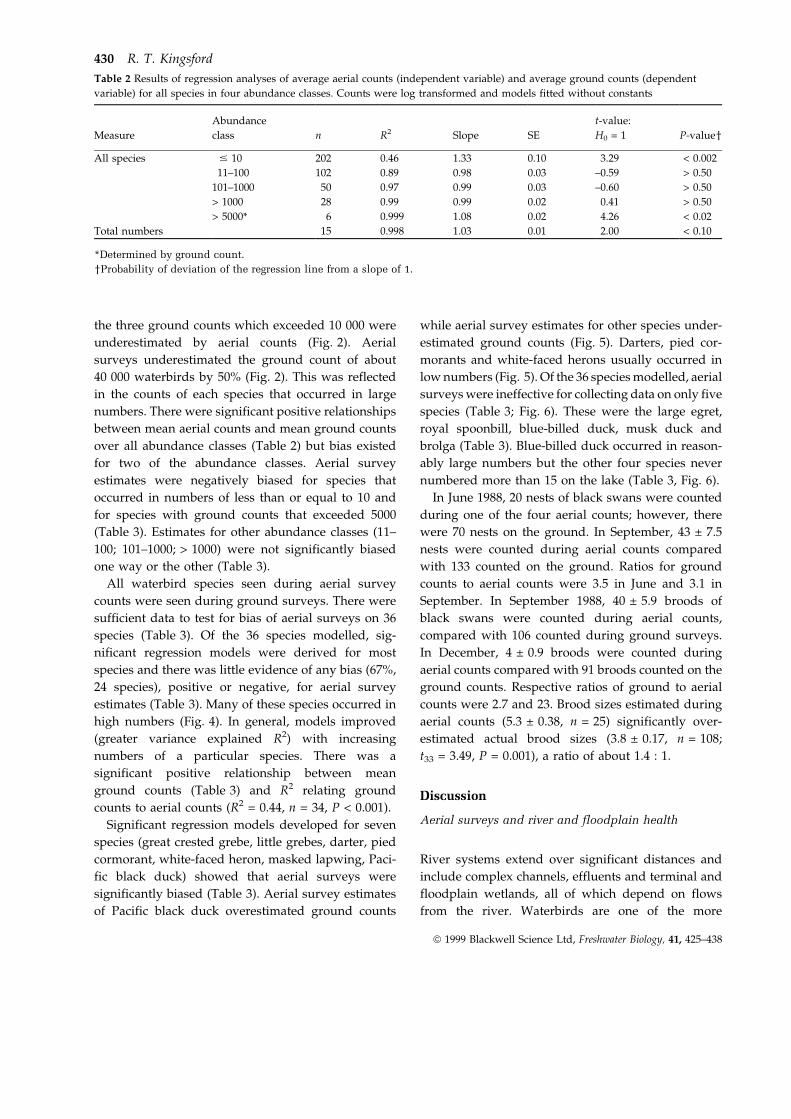
Table 2 Results of regression analyses of average aerial counts (independent variable) and average ground counts (dependent

variable) for all species in four abundance classes. Counts were log transformed and models fitted without constants

Measure

Abundance

class n R2 Slope SE

t-value:

H0 = 1 P-valueyAll species # 10 202 0.46 1.33 0.10 3.29 < 0.002

11±100 102 0.89 0.98 0.03 ±0.59 > 0.50

101±1000 50 0.97 0.99 0.03 ±0.60 > 0.50

> 1000 28 0.99 0.99 0.02 0.41 > 0.50

> 5000* 6 0.999 1.08 0.02 4.26 < 0.02

Total numbers 15 0.998 1.03 0.01 2.00 < 0.10

*Determined by ground count.

yProbability of deviation of the regression line from a slope of 1.

430 R. T. Kingsford


obvious parts of the biological community on the

wetlands. Their presence, as measured by composi-

tion and abundance, is a result of the extent of habitat

and availability of food (e.g. aquatic vegetation, fish).

These reflect the health of the system. Aerial surveys

may be a coarse measure of this community, but they

effectively tracked temporal change in the abundance

and composition of the waterbird community on Lake

Altibouka (Figs 2, 4 and 5). While Lake Altibouka is a

relatively small wetland, aerial surveys of waterbirds

have been effective over a wide range of wetlands

(Kingsford & Porter, 1993, 1994; Kingsford et al., 1994;

Kingsford & Halse, in press). They also demonstrate

spatial differences between wetlands such as whether

a wetland is saline or freshwater (Kingsford & Porter,

1994).

Table 3 Results of regression analyses of average aerial counts (independent variable) and average ground counts (dependent

variable) for all species for which there were four or more counts (n $ SE) are given for ground counts of each species. (ns, not

significant)

Waterbird n R2 Coeff. SE

t-value

H0 = 1* P-valuey Mean SE

Great crested grebe 11 0.48 3.10 0.70 3.02 < 0.05 23.9 14.65

Little grebes 13 0.69 1.77 0.34 2.26 < 0.05 199.2 64.15

Australian pelican 14 0.79 1.05 0.15 0.33 ns 203.0 144.31

Darter 7 0.88 1.81 0.27 2.99 < 0.05 5.1 2.17

Great cormorant 12 0.95 0.99 0.07 ±0.04 ns 113.9 89.92

Pied cormorant 9 0.82 1.48 0.24 1.96 < 0.10 17.4 6.69

Little black cormorant 7 0.47 0.79 0.34 ±0.61 ns 10.7 6.29

Pacific heron 6 0.89 1.35 0.22 1.69 ns 18.8 12.60

White faced heron 9 0.75 1.91 0.39 2.33 < 0.10 5.5 2.00

Large egret 8 0.34 1.68 0.89 0.55 ns 4.6 1.89

Egrets 6 0.85 1.09 0.20 0.45 ns 3.7 3.06

Straw-necked ibis 6 0.88 0.97 0.16 ±0.20 ns 13.9 7.63

Royal spoonbill 7 0.003 0.12 0.88 2.6 1.14

Yellow-billed spoonbill 8 0.80 0.99 0.19 ±0.04 ns 16.0 9.63

Black swan 16 0.99 1.03 0.03 1.24 ns 498.2 132.56

Freckled duck 9 0.93 1.10 0.11 0.91 ns 67.0 25.19

Pacific black duck 15 0.74 0.74 0.12 ±2.22 < 0.05 21.0 12.39

Grey teal 16 0.99 0.97 0.03 ±1.14 ns 1443.6 693.55

Australasian shoveler 15 0.81 1.16 0.15 1.06 ns 74.5 25.44

Pink-eared duck 14 0.98 1.01 0.04 0.14 ns 1254 433.82

Hardhead 16 0.91 0.89 0.07 ±1.55 ns 198.1 122.86

Australian wood duck 12 0.91 0.90 0.09 ±1.22 ns 126.1 52.77

Blue-billed duck 11 0.24 3.20 1.81 145.9 60.70

Musk duck 11 0.25 4.02 2.20 6.9 2.79

Eurasian coot 15 0.98 1.07 0.04 1.61 ns 3860.9 1356.78

Brolga 7 0.25 0.76 0.53 1.62 0.28

Masked lapwing 13 0.78 1.47 0.23 2.08 < 0.10 17.3 5.35

Banded lapwing 5 0.65 2.64 0.98 1.68 ns 8.5 5.88

Black-winged stilt 15 0.86 0.92 0.10 ±0.87 ns 54.0 20.19

Banded stilt 4 0.82 1.14 0.31 0.45 ns 24.2 19.01

Red-necked avocet 15 0.93 1.01 0.08 0.16 ns 77.5 31.21

Small waders 13 0.73 0.84 0.15 ±0.08 ns 136.4 57.10

Silver gull 16 0.97 1.06 0.05 1.33 ns 114.7 26.21

Whiskered tern 12 0.87 1.16 0.13 1.20 ns 112.1 38.45

Gull-billed tern 11 0.62 1.35 0.34 1.05 ns 24.2 7.98

Caspian tern 14 0.65 0.96 0.20 ±0.23 ns 16.6 5.75

*Tests bias on only those species where a significant relationship was found between aerial and ground counts (i.e. H0 ¹ 0,

P < 0.10).

ySpecies with significant bias between aerial and ground counts. A positive t-value and significant probability shows aerial counts

underestimated ground counts.



The ability to effectively monitor many species

simultaneously (Fig. 4) allows observers the flexibility

of detecting changes to the suite of species which

reflect river and floodplain health. The abundance of

feeding guilds of waterbirds can be a measure of other

biological aspects of the wetland. For example, the

composition of waterbird communities reflected fish

and shrimp abundance on Lake Numalla and inverte-

brates and aquatic macrophytes abundance on Lake

Wyara (about 200 km north-east of Lake Altibouka)

(Kingsford & Porter, 1994). Aerial surveys also allow

more than one aerial count to be obtained relatively

easily because of the discrete nature of wetland

habitat. Given the relatively large time and financial

cost of doing ground counts, this represents a distinct

advantage. Differences among counts may be com-

pared to differences within counts (Green, 1979; p. 27).

As well, extra aerial surveys detect more species

occurring in low numbers and guard against equip-

ment failure (data for five aerial surveys were lost in

this study).

Dams and diversion of water alter flow regimes

(Ligon, Dietrich & Trush, 1995) and may significantly

impact on these systems (Maheshwari, Walker &

McMahon, 1995). The management of this complex

longitudinal and lateral system demands a landscape

approach (Sparks, 1995). The most significant anthro-

pogenic impacts occur at this large scale and it is often

the wetlands dependent on river flows that have been

most affected, particularly by diversion of water from

rivers (Micklin, 1988; Bren, 1992; Weins, Patten &

Botkin, 1993; Lemly, 1994; Kingsford & Thomas, 1995;

Thomas, 1995) and river management (Tamisier &

Grillas, 1994; Gunderson, Light & Holling, 1995).

Wetland management more often depends on regio-

nal management than site management (Barendregt,

Wassen & Schot, 1995). Waterbirds are an obvious

biological component of a wetland and aerial surveys

can provide a rapid and useful method for estimating

their abundance and diversity.

Biological studies of rivers are often limited to a fine

scale (< 100 m2) because of the complexities of data

Fig. 4 Numbers of waterbirds of species for which aerial surveys were not effective; data are means (with standard errors) of four

aerial counts (dotted line, squares) and three ground counts (continuous line, circles) per trip; trips were three-monthly (June 1987±

September 1990), and in March 1993 (I), June 1994 (II) and March 1995 (III). There was no significant relationship between aerial

survey estimates and ground counts (P > 0.05).

432 R. T. Kingsford


collection and spatial and temporal variability in the

abundance of aquatic organisms. Aerial surveys of

waterbirds are less restrictive. What aerial surveys

lack in precision and accuracy (Tables 1±3), they more

than make up for in advantages of spatial and

temporal scale. They can cover significant survey

areas in a relatively short amount of time. This has

allowed managers and scientists to design aerial

surveys across large landscape areas (Henny et al.,

1972; Joensen, 1974). About 1500 wetlands are

surveyed each year in an aerial survey of more than

50 species of waterbirds across about 10% of eastern

Australia (Braithwaite et al., 1986; Kingsford, Tully &

Davis, 1997).

The temporal scale is especially important for

countries such as Australia with extremely variable

rivers (McMahon et al., 1992; Walker, Puckridge &

Blanch, 1997; Puckridge et al., 1998) and unpredictable

rainfall (Pittock, 1975). Separating climatic stochasti-

cally from anthropogenic impact becomes a challenge.

Measures of river health will often need to extend for

large periods of time (years to decades) to clearly

identify if a river is actually in good health and

whether remediation is necessary. Aerial surveys of

waterbirds may be done for long periods. For

example, aerial surveys of eastern Australia

(Braithwaite et al., 1986) have been performed every

year since 1983. They provide opportunities for

measuring river health on dependent wetlands with

catchment scale implications (Kingsford & Thomas,

1995; DLWC & NPWS, 1996). Because whole wetlands

may be surveyed, perhaps even all key wetlands

within a catchment, aerial surveys can contribute

significantly to river management at the scale of the

whole river.

Accuracy and precision of aerial surveys

Effectiveness of aerial survey of waterbirds deserves

discussion. The applicability of this measure for

Fig. 5 Means of three ground counts (continuous line, circles) and four aerial counts (dotted line, squares), with standard errors, for

waterbird species for which aerial surveys were negatively biased (great crested grebe, little grebes, darter, pied cormorant, white-

faced heron and masked lapwing) and positively biased (Pacific black duck) compared to ground surveys (P < 0.10). Trips were three-

monthly (June 1987±September 1990), and in March 1993 (I), June 1994 (II) and March 1995 (III).



Fig. 6 Means of three ground counts (continuous line, circles) and four aerial counts (dotted line, squares), with standard errors, for

waterbird species for which aerial surveys were not biased compared to ground surveys (P > 0.05); trips were three-monthly (June

1987±September 1990), and in March 1993 (I), June 1994 (II) and March 1995 (III).

434 R. T. Kingsford


determining river or floodplain health depends on its

accuracy and precision in relation to spatial and

temporal change in the waterbird community. Aerial

surveys of waterbird communities performed reason-

ably well compared with the more time consuming

and possibly more accurate ground counts. For 31 out

of 36 waterbird species for which models were

developed, aerial surveys tracked changes detected

during ground surveys on Lake Altibouka (Table 3).

The relationship between ground and aerial counts

was strongest for species that occurred in large

numbers (Table 3; Fig. 4).

Aerial surveys were also reasonably precise, parti-

cularly for species that occurred in large numbers

(Table 1). They had lower precision than some ground

counts (Table 1) which was not surprising given that

two observers had to estimate between 500 and 40 000

waterbirds, including up to 45 waterbird species, in

about two and a half minutes. Many factors contribute

to problems in estimating and identifying birds

during aerial surveys: species' characteristics, cover,

density of birds, phenology, seasonal changes in

water levels and changes in crew members (Henny

et al., 1972). Concentration on a few waterbird species

might increase precision (Watson, Freeman & Jolly,

1969) but would result in substantial loss of informa-

tion for the rest of the waterbird community.

There were some difficulties with aerial surveys.

They underestimated abundance when a species

occurred in numbers of less than 10 or more than

5000 (Table 2). For five species which occurred in low

numbers (Fig. 5), no model could be found that would

relate ground to aerial counts (Table 3). Similarly,

masked lapwings, which usually occur singly or in

pairs, were underestimated (Fig. 5; Table 3). For

another four species, aerial surveys significantly

underestimated numbers (Fig. 5; Table 3). Great

crested grebe, little grebes, blue-billed duck and

musk duck probably dived in response to the aircraft

because observers often saw ripples or splashes in the

water directly below the aircraft and large (> 50)

compact flocks of little grebes diving in the distance.

One result was at odds with the pattern of negative

bias. Aerial surveys consistently overestimated the

numbers of Pacific black duck counted on the ground

(Fig. 5); possibly some were Australasian shoveler

which are similar when viewed from above.

At large concentrations, the negative bias was

particularly obvious for two species: Eurasian coot

and grey teal (Fig. 4). This translated into a negative

bias for total numbers (Table 2). At its most extreme,

this difference meant a 50% underestimate of total

numbers of waterbirds on the lake in December 1988

(Fig. 2). Negative bias of large aerial counts was

probably not linear. Such density dependent bias has

been detected in other surveys of waterbirds (Joensen,

1968, 1974; Prater, 1979; Dexter, 1990). Most aerial

surveys of waterbirds suffer a negative bias relative to

ground counts (Diem & Lu, 1960; Stott & Olson, 1972;

Broome, 1985; Johnson, Pollock & Montalbano, 1989;

Morton et al., 1990a,b) or photographic counts (Bayliss

& Yeomans, 1990). Even when aerial counts of

waterbirds have exceeded ground counts, this has

been attributed to the problems of counting water-

birds from the ground (Heusmann, 1990).

Ground counting, which can also be done from a

boat, is often believed to be accurate and without

error. Studies reporting the accuracy of aerial surveys

of waterbirds have used ground counts more than a

day later or earlier than aerial counts but have given

no estimate of daily variability of ground counts

(Diem & Lu, 1960; Martin, Pospahala & Nichols, 1979;

Broome, 1985; Morton et al., 1990a,b). Precision of

ground counts is usually unknown (Broome, 1985;

Johnson et al., 1989; Heusmann, 1990). Lake Altibouka

was ideal for ground counts because of its small size

and lack of surface vegetation. Much of the impreci-

sion in ground counts (Table 1) was probably related

to daily variability although factors such as birds

obscuring each other, birds missed while diving, glare

off the water and haze and, possibly, observer fatigue

all contributed. Sometimes, distance to the opposite

shoreline also made identification difficult. Daily

variability was most apparent for species that

occurred in small numbers. These species may be

using the wetland habitat as a stop over on their way

to more suitable habitat.

If ground counts are to be used, some measure of

precision should be attempted. Ground counts on

many wetlands are impractical because of size,

amount of vegetation and waterbird abundance.

Also, where numbers of waterbirds occur in particu-

larly large numbers (> 40 000) or on large lakes

(Kingsford et al., 1994), it would be virtually impos-

sible to do ground counts. It took three of us eight

hours to do ground counts of Lake Altibouka when

there were 40 000 birds. Disturbance resulting in

double counts (Caughley, 1977; p. 38) is also a



significant problem. The importance of obtaining

more than one count to measure temporal or spatial

differences compounds the problem.

Conclusion

Aerial surveys can be used to collect data on water-

bird abundance for up to 50 different species. Because

the method is quick and inexpensive compared with

ground counts, large areas may be surveyed, provid-

ing information at a landscape scale. Unlike aerial and

ground surveys of other animal populations, a whole

wetland may be surveyed, eliminating the need for

sampling. More than one aerial survey of the same

birds on a wetland allows estimation of precision. One

of their most significant advantages is that the results

of aerial surveys may be applied to the management

of an entire river and its floodplain. Such information

is more easily incorporated by river managers who

tend to manage at the scale of the catchment. The

more indices we have of river and floodplain health at

the catchment scale, the more likely it is that results of

studies by ecologists will be implemented by river

managers.

Acknowledgements

J.L. Porter, J. Smith, J. Holmes and W. Lawler assisted

in the field. N. Weber helped with statistical analyses.

N. Weber, S.V. Briggs, S. Cairns and R.C. Kingsford

reviewed an earlier draft of this manuscript. Susan

Davis helped with the figures. This research was

supported by the New South Wales National Parks

and Wildlife Service.

References

Allan J.D. & Flecker A.S. (1993) Biodiversity conservation

in running waters. Bioscience, 43, 32±43.

Andrew N.L. & Mapstone B.D. (1987) Sampling and the

description of spatial pattern in marine ecology.

Oceanography Marine Biology Annual Review, 25, 39±

90.

Barendregt A., Wassen M.J. & Schot P.P. (1995) Hydro-

logical systems beyond a nature reserve, the major

problem in wetland conservation of Naardermeer (the

Netherlands). Biological Conservation, 72, 393±405.

Bayliss P. & Yeomans K.M. (1990) Use of low-level aerial

photography to correct bias in aerial survey estimates

of magpie goose and whistling duck density in the

Northern Territory. Australian Wildlife Research, 17, 1±

10.

Braithwaite L.W., Maher M., Briggs S.V. & Parker B.S.

(1986) An aerial survey of three game species of

waterfowl (Family Anatidae) in eastern Australia.

Australian Wildlife Research, 13, 213±223.

Bren L.J. (1992) Tree invasion of an intermittent wetland

in relation to changes in the flooding frequency of the

River Murray, Australia. Australian Journal of Ecology,

17, 395±408.

Briggs S.V. & Maher M.T. (1985) Limnological studies of

waterfowl habitat in south-western New South Wales.

II. Aquatic macrophyte productivity. Australian Journal

of Marine and Freshwater Research, 36, 59±67.

Briggs S.V., Thornton S.A. & Lawler W.G. (1997)

Relationships between hydrological control of river

red gum wetlands and waterbird breeding. Emu, 97,

31±42.

Broome L.S. (1985) Sightability as a factor in aerial survey

of bird species and communities. Australian Wildlife

Research, 12, 57±67.

Caughley G. (1977) Analysis of Vertebrate Populations. John

Wiley & Sons, New York.

Conroy M.J., Goldsberry J.R., Hines J.E. & Stotts D.B.

(1988) Evaluation of aerial transect surveys for winter-

ing American black ducks. Journal of Wildlife Manage-

ment, 52, 694±703.

Dexter N. (1990) Density dependent bias in aerial counts

of magpie goose nests. Australian Wildlife Research, 17,

447±451.

Diem K.L. & Lu K.H. (1960) Factors influencing water-

fowl censuses in the parklands, Alberta. Canadian

Journal of Wildlife Management, 24, 113±133.

DLWC & N.P.W.S. (1996) Macquarie Marshes Water

Management Plan 1996. National Parks and Wildlife

Service and Department of Land and Water Conserva-

tion, Sydney, Australia.

EPA (1997) Proposed Interim Environmental Objectives for

NSW Waters. Environment Protection Authority,

Chatswood, Sydney.

Green R.H. (1979) Sampling Design and Statistical Methods

for Environmental Biologists. John Wiley & Sons, New

York.

Gunderson L.H., Light S.S. & Holling C.S. (1995) Lessons

from the Everglades. Bioscience, S66±S:73.

Henny C.J., Anderson D.R. & Pospahala R.S. (1972) Aerial

Surveys of Waterfowl Production in North America, 1955±

71. US Fish. Wildl. Serv. Spec. Sci. Report, Wildl. no.

160.

Heusmann H.W. (1990) Evaluation of air/ground count

comparisons for wintering American black ducks.

Wildlife Society Bulletin, 18, 377±381.

Howard G.W. & Aspinwall D.R. (1984) Aerial censuses of

436 R. T. Kingsford


shoebills, saddlebilled storks and wattled cranes at the

Bangweulu swamps and Kafue Flats, Zambia. Ostrich,

55, 207±212.

Joensen A.H. (1968) Wildfowl counts in Denmark in

November 1967 and January 1968 Ð methods and

results. Danish Review of Game Biology, 5, 1±70.

Joensen A.H. (1974) Wildfowl populations in Denmark

1965±73. Danish Review of Game Biology, 9, 1±206.

Johnson D.H. (1989) An empirical Bayes approach to

analyzing recurring animal surveys. Ecology, 70, 945±

952.

Johnson F.A., Pollock K.H. & Montalbano F. III (1989)

Visibility bias in aerial surveys of mottled ducks.

Wildlife Society Bulletin, 17, 222±227.

Karr J.R. (1981) Assessment of biotic integrity using fish

communities. Fisheries, 6, 21±26.

Kingsford R.T., Bedward M. & Porter J.L. (1994) Wetlands

and Waterbirds in North-western New South Wales. NSW

National Parks and Wildlife Service, Sydney, Australia,

Occasional Paper no. 19, 105 pp.

Kingsford R.T. & Halse S.A. (in press) Waterbirds as the

`flagship' for the conservation of arid zone wetlands in

Australia? Wetlands for the Future. Proceedings of

INTECOL's V International Wetlands Conference (Eds

A.J. McComb and J.A. Davis), Gleneagle Press,

Adelaide, Australia.

Kingsford R.T. & Porter J.L. (1993) Waterbirds of Lake

Eyre, Australia. Biological Conservation, 65, 141±151.

Kingsford R.T. & Porter J.L. (1994) Waterbirds on an

adjacent freshwater lake and salt lake in arid Australia.

Biological Conservation, 69, 219±228.

Kingsford R.T. & Thomas R.F. (1995) The Macquarie

Marshes in arid Australia and their waterbirds: a 50

year history of decline. Environmental Management, 19,

867±878.

Kingsford R.T., Tully S. & Davis S.T. (1997) Aerial Surveys

of Wetland Birds in Eastern Australia ± October 1994 and

1995. NSW National Parks and Wildlife Service,

Sydney, Australia, Occasional Paper no. 28, 34 pp.

Lemly A.D. (1994) Irrigated agriculture and freshwater

wetland: a struggle for coexistence in the western

United States. Wetlands Ecology and Management, 3, 3±

15.

Ligon F.K., Dietrich W.E. & Trush W.J. (1995) Down-

stream ecological effects of dams. Bioscience, 45, 183±

192.

Maher M. & Carpenter S.M. (1984) Benthic studies of

waterfowl breeding habitat in south-western New

South Wales. II. Chironomid populations. Australian

Journal of Marine and Freshwater Research, 35, 97±

110.

Maheshwari B.L., Walker K.F. & McMahon T.A. (1995)

Effects of regulation on the flow regime of the River

Murray, Australia. Regulated Rivers ± Research and

Management, 10, 15±38.

Martin F.D., Pospahala R.S. & Nichols J.D. (1979) In

Assessment and Population Management of North Amer-

ican Migratory Birds. Environmental Biomonitoring, As-

sessment, Prediction and Management Ð Certain Case

Studies and Related Quantitative Issues. pp. 187±239.

International Co-operative Publication House, Mary-

land.

McMahon T.A., Finlayson B.L., Haines A.T. & Srikanthan

R. (1992) Global Runoff: Continental Comparisons of

Annual Flows and Peak Discharges. Cremlingen-Destedt:

Cantena Vertlag, Germany.

Micklin P.P. (1988) Desiccation of the Aral Sea: a water

management disaster in the Soviet Union. Science, 241,

1170±1176.

Morton S.R., Brennan K.G. & Armstrong M.D. (1990a)

Distribution and abundance of ducks in the Alligator

rivers region, Northern Territory. Australian Wildlife

Research, 17, 573±590.

Morton S.R., Brennan K.G. & Armstrong M.D. (1990b)

Distribution and abundance of magpie geese, Anser-

anas semipalmata in the Alligator rivers region, North-

ern Territory. Australian Journal of Ecology, 15, 307±320.

Nilsson L. (1975) Midwinter distribution and numbers of

Swedish Anatidae. Ornis Scandinavica, 6, 83±107.

Pimmental D., Houser J., Preiss E., White O., Fang H.,

Mesnick L., Barsky T., Tariche S., Schreck J. & Alpert S.

(1997) Water resources: agriculture, the environment

and society. Bioscience, 47, 97±106.

Pittock A.B. (1975) Climatic change and the patterns of

variation in Australian rainfall. Search, 6, 498±504.

Postel S.L., Daily G.C. & Ehrlich P.R. (1996) Human

appropriation of renewable fresh water. Science, 271,

785±788.

Prater A.J. (1979) Trends in accuracy of counting birds.

Bird Study, 26, 198±200.

Puckridge J.T., Sheldon F., Walker K.F. & Boulton A.J.

(1998) Flow variability and the ecology of large rivers.

Marine and Freshwater Research, 49, 55±72.

Ruello N.V. (1976) Observations on some massive fish

kills in Lake Eyre. Australian Journal of Marine and

Freshwater Research, 27, 667±672.

Sokal R.R. & Rohlf F.J. (1981) Biometry: the Principles and

Practice of Statistics on Biological Research, 2nd edn. W.H.

Freeman and Co., San Francisco, CA.

Sparks R.E. (1995) Need for ecosystem management of

large rivers and their floodplains. Bioscience, 45, 168±

182.

Stott R.S. & Olson D.P. (1972) An evaluation of waterfowl

surveys on the New Hampshire coastline. Journal of

Wildlife Management, 36, 468±477.

Tamisier A. & Grillas P. (1994) A review of habitat



changes in the Camargue: an assessment of the effects

of the loss of biological diversity on the wintering

waterfowl community. Biological Conservation, 70, 39±

47.

Thomas D.H.L. (1995) Artisanal fishing and environ-

mental change in a Nigerian floodplain wetland.

Environmental Conservation, 22, 117.

Thoms M.C. (1998) Floodplain wetlands: transient

storage areas of sediments and pollutants. Wetlands in

a Dryland: Understanding Management (Ed. W.D. Wil-

liams), pp. 205±216. Environment Australia, Biodiver-

sity Group, Canberra.

Walker K.F., Puckridge J.T. & Blanch S.J. (1997) Irrigation

development on Cooper Creek, central Australia ±

prospects for a regulated economy in a boom-and-bust

ecology. Aquatic Conservation: Marine and Freshwater

Ecosystems, 7, 63±73.

Watson R.H., Freeman G., H. & Jolly G.M. (1969) Some

indoor experiments to simulate problems in aerial

censusing. East African Agricultural Forestry Journal, 34,

56±59.

Weins J.A., Patten D.T. & Botkin D.B. (1993) Assessing

ecological impact assessment: lessons from Mono Lake,

California. Ecological Applications, 3, 595±609.

Wilkinson L., Hill M., Welna J.P. & Birkenbeuel G.K.

(1992) Systat for Windows: Statistics, Version 5., Systat

Incorporated, Evanston, IL.

Zar J.H. (1984) Biostatistical Analysis, 2nd edn. Prentice

Hall Inc, Englewood Cliffs, NJ.

(Manuscript accepted September 1998)

438 R. T. Kingsford


aerial survey of waterbirds on wetlands as a measure of river and floodplain health

Documents