aec terrain step by step tutorials 2: earthwork in area grading (level pads) step 1: follow step 1...

AEC Terrain Step by Step Tutorials

Tutorial 1: Generation of Terrain and Contours

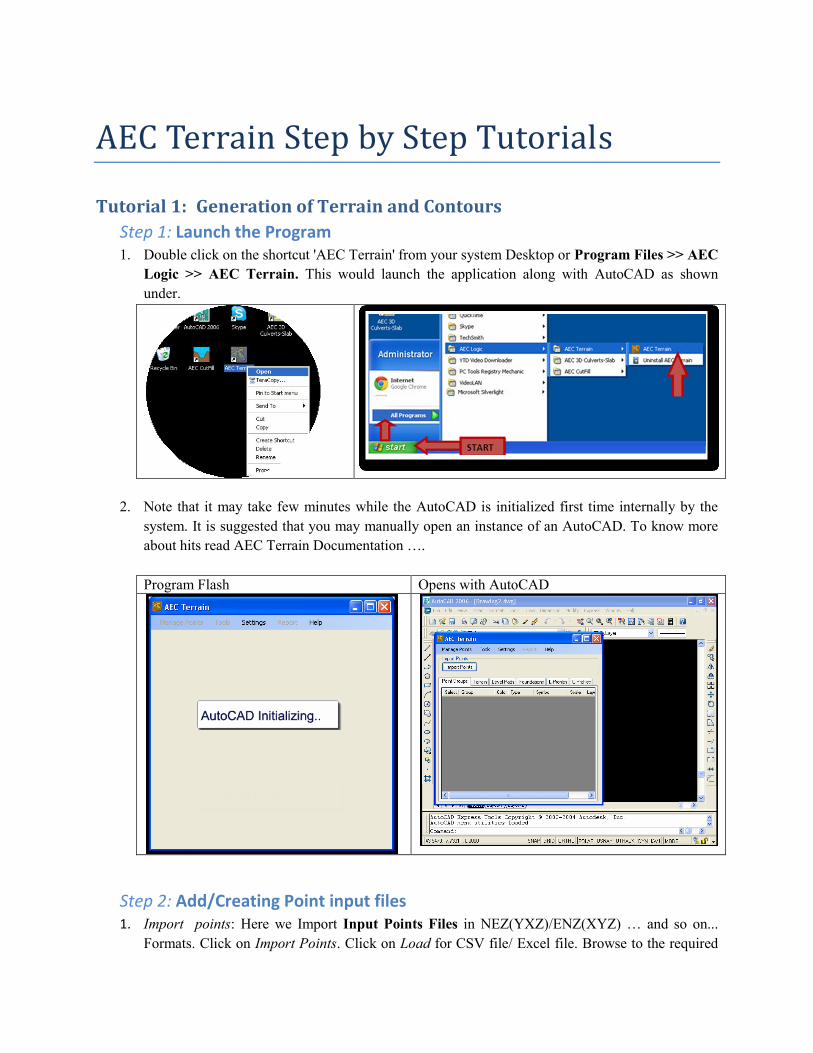
Step 1: Launch the Program 1. Double click on the shortcut 'AEC Terrain' from your system Desktop or Program Files >> AEC

Logic >> AEC Terrain. This would launch the application along with AutoCAD as shown

under.

2. Note that it may take few minutes while the AutoCAD is initialized first time internally by the

system. It is suggested that you may manually open an instance of an AutoCAD. To know more

about hits read AEC Terrain Documentation ….

Program Flash Opens with AutoCAD

Step 2: Add/Creating Point input files 1. Import points: Here we Import Input Points Files in NEZ(YXZ)/ENZ(XYZ) … and so on...

Formats. Click on Import Points. Click on Load for CSV file/ Excel file. Browse to the required

file location. (File should be in CSV format/Excel format, that is, .csv/.xls extension). The CSV

file shown below is available in Sample Files at Program Files >> AEC Logic >> AEC Terrain

>> Samples >> Example 2 Points NEZ OR YXZ.

Note 1: File Formats

Input Points Files could be in NEZ(YXZ)/ENZ(XYZ) if imported from other sources and the file

should be in CSV/Excel format, that is, .csv/ .xls extension.

Click command button then click on command button to load Input

Points File whether the Points file is in CSV or Excel Format. Select Example 2 Points NEZ OR

YXZ then click on

2.

Step 3: Plot Points on AutoCAD 3. Import Points (OR plot on AutoCAD): After the file management (adding and deleting files); click

this command to post/plot points on to the AutoCAD Editor form the point files shown in the

File List Box .

CSV File Format Excel Format

4. Verify point data on Main Form >> Point Groups Tab:

Step 4: Generate Terrain Surface 5. Click on Terrain Tab and see that Scan radius is set to 100.

6. Click Generate Surface: Triangulated Irregular Network (TIN) representing surface derived

from irregularly spaced sample points is generated as under. Without having the Draw

Contour checked we have the surface generated as under.

7. To View the terrain as under use AutoCAD commands >> View menu >> Shade >> Flat

Shaded.

Step 5: Generate Contours 8. To generate contour lines check the Draw Contour check box and click the Generate command

as said above again.

Step 6: Find Volume of Thickened Surface 3. Let us take some example of an area with a point file with us and import them to the AutoCAD,

draw the TIN surface as shown below. The Thickened surface volume for 10 meter height is

shown as under.

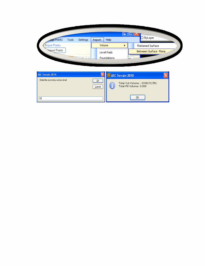
Step 7: Find Volume between Surface & Plane 4. Volume between the surface and a plane is calculated by the program and the example values are

shown below for the above said surface.

Tutorial 2: Earthwork in Area Grading (Level Pads)

Step 1: Follow Step 1 of Tutorial 1



Step 4: Go to Level Pads Tab 1. AEC Terrain >> Click Level Pads Tab

Step 5: Draw a Closed Polyline(s) 2. Draw Closed polylines around an area/region where you propose to draw a level pads.

Note 1: Multiple pads

3. Multiple level pads can also be drawn by multiple selection of closed polylines.

4. Note: The Polyline should fall within the extent of the point files/TIN surface boundary.

Step 6: Select the Polyline(s) Boundaries 5. Select the boundaries so drawn for the proposed area leveling.

6. The Boundary lines (Selected closed polylines) shall be listed in the Data Grid with captured data

from the AutoCAD, like minimum and maximum levels with naming as B1, B2 and B3 and so on..

as boundaries. These boundaries can be renamed as the user wishes them to be.

Step 7: Set the proposed final Level(s) 7. Enter a level to which the area needs to be leveled as per the project requirement.

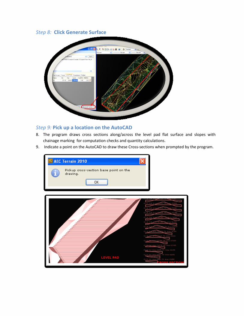
Step 8: Click Generate Surface

Step 9: Pick up a location on the AutoCAD 8. The program draws cross sections along/across the level pad flat surface and slopes with

chainage marking for computation checks and quantity calculations.

9. Indicate a point on the AutoCAD to draw these Cross-sections when prompted by the program.

Note 1: Graded surface Coordinates

10. Program writes a file with coordinates of the new flat surface LevelPads_Coordinates.csv. The

file will be saved in the Input folder. The coordinates shall be in coordinates in NEZ format. This

file when plotted again would make a flat TIN surface as shown in the image below. Click on OK

Note 2: Output CSV file format

11. The output file format shall be as under.

N E Z

657826.8 164613.8 257.713

657828.0 164602.5 260.128

657825.5 164606.8 260.199

657825.6 164583.6 253.392

657827.9 164606.2 260.258

657850.0 164593.3 250.894

657843.2 164599.6 254.374

657867.4 164642.4 260.269

657870.3 164638.9 260.319

657858.0 164631.5 260.385

657871.0 164613.5 251.191

657831.4 164632.5 252.050

657860.4 164606.7 252.092

657844.2 164631.7 256.288

Step 10: Area/Volume Calculations 12. Go to Reports >> Click Level Pads to generate area report. After the Generation of the Level

Pads Cut-fill area report is shown below cross-section wise. The report may be exported to Excel

Format and volumes be calculated as per chainage intervals.

Step 11: More examples of Area Grading 13. Most commonly used functional requirements by civil engineering project constructions are

shown under. The program can be used for different applications in different situations as the

construction site demands.

14. Slopes definitions can be set for the area leveling. Whereas the project may require longitudinal

slopes, cross slopes, curve definitions if an alignments is required to be designed for different

applications.

Flattening long areas Earthen dams, Embankments

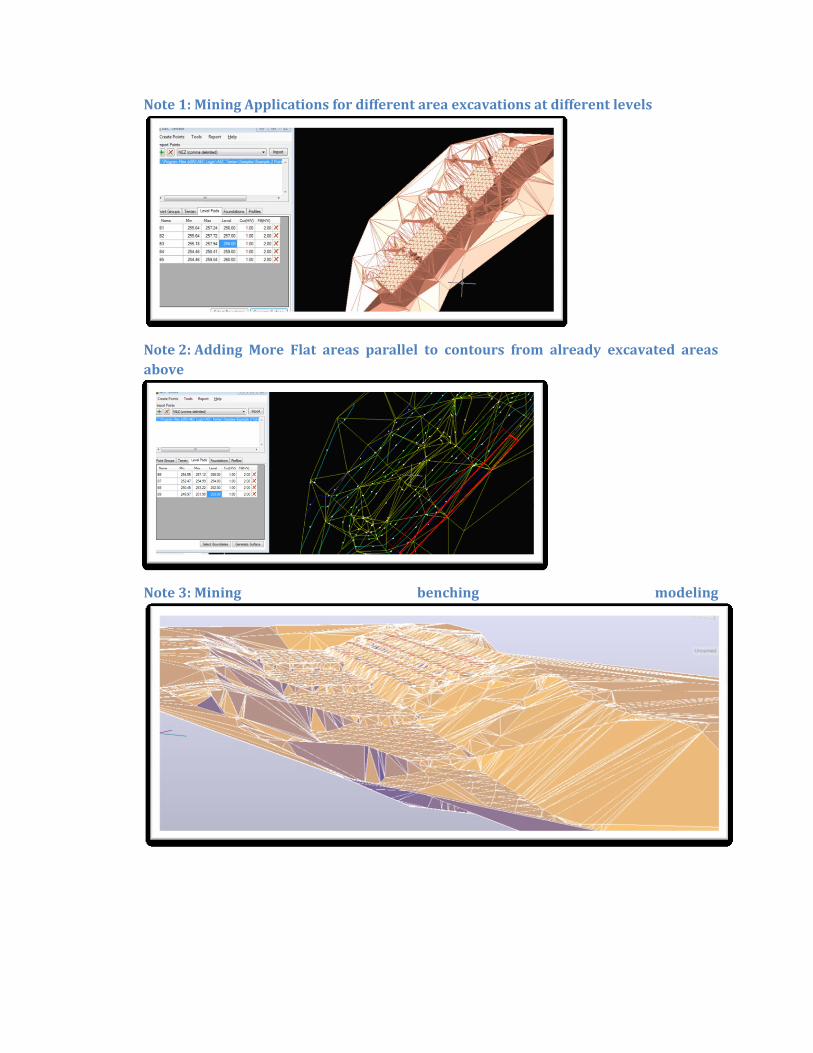
Note 1: Mining Applications for different area excavations at different levels

Note 2: Adding More Flat areas parallel to contours from already excavated areas

above

Note 3: Mining benching modeling

Note 4: Mining Applications with surfaces at different stages:

The Combined and cumulative excavated areas containing multi levels pads for real time mining

applications is shown as under. Original surface, Original and final surface interlaced and final

surface are shown separately in the following images.

Note 5: Multiple level pads either in cut or in fill:

Note 6: Drains as Area Excavation

Note 7: Canals

Tutorial 3: Earthwork for Foundation Excavations




Step 4: Click on Foundations Tab 1. On AEC Terrain main form click on the Foundations Tab as shown under.

Note 1: Foundations on irregular surface

2. This is the most complicated modeling in civil engineering field. If this is mastered, construction

becomes simplified and the results expected are met drastically reducing prolonged drainage

problems etc after the infrastructure is built.

3. The solution would solve commonly encountered problems on site. This is useful for either

making excavations, see the extents of slope influence on the adjacent structures and so on.

4. Follow the same process as explained in above steps up to selection of point input file in

example 2 under Samples folder.

Step 5: Draw the Polyline(s) 5. Draw closed polylines on the AutoCAD editor directly or copy from another AutoCAD file for the

foundations pits desired in the similar fashion as explained in Tutorial 2 Earthwork in Area

Leveling. The closed polylines may be for example, 6 polylines of 3X4 m size each.

6. Foundations excavations are modeled on the TIN surface with new TIN surface generated and

output files generated

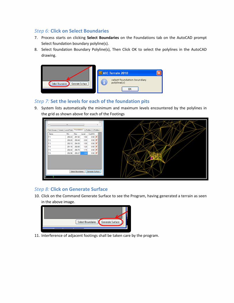
Step 6: Click on Select Boundaries 7. Process starts on clicking Select Boundaries on the Foundations tab on the AutoCAD prompt

Select foundation boundary polyline(s).

8. Select foundation Boundary Polyline(s), Then Click OK to select the polylines in the AutoCAD

drawing.

Step 7: Set the levels for each of the foundation pits 9. System lists automatically the minimum and maximum levels encountered by the polylines in

the grid as shown above for each of the Footings

Step 8: Click on Generate Surface 10. Click on the Command Generate Surface to see the Program, having generated a terrain as seen

in the above image.

11. Interference of adjacent footings shall be taken care by the program.

Note 1: Shaded Foundations on DWG TrueView

Note 2: Shaded Foundations on DWG TrueView with partial top/bottom view

Note 3: Shaded Foundations on DWG TrueView with partial bottom view

Note 4: Foundations on leveled/finished surface

Step 9: Foundation Excavation Volumes 12. Volume Report for the Foundations shown below.

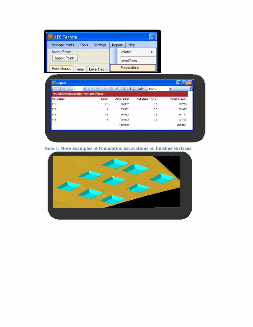
Note 1: More examples of Foundation excavations on finished surfaces

Tutorial 4: Surface Profiles along Project Alignments 1. To found engineering structures like buildings, culverts, bridges and similar structures in to the

ground we need to know the extent and level of excavation need to be verified and fit on to the

terrain for several practical seating. This feature enables such requirement and reports volume

of excavations.

2. We may need to generate profiles along a straight line, circular/arc paths (needs to be drawn in

polyline format) and so on. We need to find the surface profile of the ground along such paths.

AEC Terrain draws such profile along the defined path




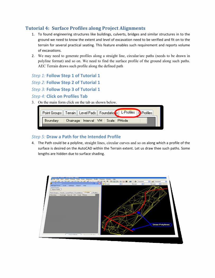
Step 4: Click on Profiles Tab 3. On the main form click on the tab as shown below.

Step 5: Draw a Path for the Intended Profile 4. The Path could be a polyline, straight lines, circular curves and so on along which a profile of the

surface is desired on the AutoCAD within the Terrain extent. Let us draw thee such paths. Some

lengths are hidden due to surface shading.

Step 6: Select the Paths 5. Click on the Select Paths command

Step 7: Select all Polylines 6. Select all path lines on the AutoCAD on the following prompt.

7. Path data is generated and written to the program grid.

Step 8: Set Profile Modes 8. Three possible modes (PMode), namely Intervals, Nodes and both Nodes & Intervals can be set

for each path. Here we can also set the Start Chainage (for example the path may have a start

chainage other than 0.00), Interval and Vertical magnification (VM) and Scale.

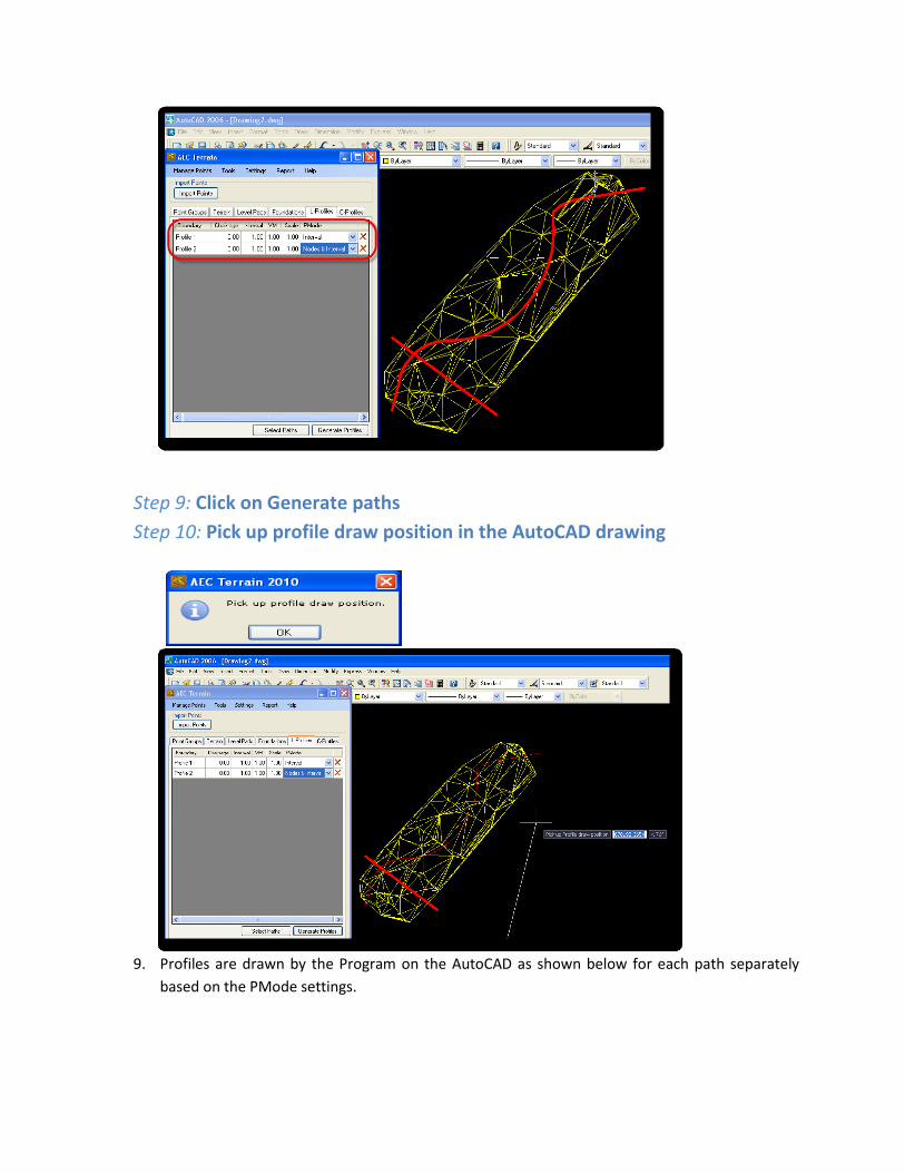
Step 9: Click on Generate paths

Step 10: Pick up profile draw position in the AutoCAD drawing

9. Profiles are drawn by the Program on the AutoCAD as shown below for each path separately

based on the PMode settings.

10. Profile Drawing in enlarged view is as under.

11. Program generates output files for all the three profiles with coordinates in CSV format. The

data CSV output files for the profile generation are as shown as under.

12. These path coordinates and cross sections may be required for many engineering structures

during, design, construction and fitment issues on construction sites. Height of structures at

each node/interval may decide the design requirements and sufficiency and/or economizing

issues given a terrain point file.

Tutorial 5: Cross Profiles along Project Alignments




Step 4: Go to C-Profiles Tab

Step 5: Draw a Polyline path

Step 6: Select path 13. Select path line shown in red color below (Selected Line should be a Polyline) and click on

Generate profile as shown in the image.

Step 7: Save the Output File 14. Cross section file to be saved at the desired project folder location. The file contains the

coordinates of all the generated from the terrain.

Step 8: Pick up a position

15. Pick a position on the AutoCAD editor on the program prompt to place the cross sections being

generated.

Step 9: You have done it 16. The generated Cross sections are seen as under on the AutoCAD Screen.

17. Enlarged each Cross section would look as under.

18. The Output CSV file containing the data of the each cross section is generated as under. The

Longitudinal and cross intervals are explained in the above paragraphs.

Cross section @ Chainage 20.00mts

Cross section @ Chainage 28.969mts

Tutorial 6: Customizing AEC Terrain Environment

Step 1: Settings>> Settings

Step 2: Customizing Default Output Parameters 19. General Tab:

a) In the Tools >> Settings >> General tab >>Text Height: System by default sets this as 0.3

m since the contours are at 1 meter intervals and close look at the contours will give

better view. Depending on the user functionality this may be set at higher or lower

values.

b) In the Tools >> Settings >> General tab >>Initial Surface Color: Set as desired color.

System sets by default green as initial color indicating original surface

c) In the Tools >> Settings >> General tab >>Level Pad Surface Color: This may be set as

required by the users to suit their requirements

d) In the Tools >> Settings >> General tab >> Foundation Surface Color: This may be set as

required by the users to suit their requirements

20. Level Pads Tab: You may require in your project to make foundation pits at several places on the

terrain and the settings so required may be entered here for the Program to draw. Enter the

Cross section intervals as per the convenience, show the project file path for the Coordinates file

(CSV File) to be written in NEZ format. If you want the Cross sections in the AutoCAD drawings

then do check the box.

21. Foundations Tab: You may require in your project to make foundation pits at several places on

the terrain and the settings so required may be entered here for the application to draw.

(a) Excavation Depth: By Default the AEC Terrain shall make your Foundation depths at

this setting until you set a new value.

(b) Cut Slope: The Application assumes the slope set here for generating the surfaces

until you set a new value

(c) You may need to write the coordinates of your new foundation surface to a file

location for further managing. Define the default path for writing them to that

location.

22. L-Profiles Tab: You may need your program to draw your surface profiles with a graphic grid

behind. The default values to create such graphic grid profiles are set here.

(a) Section Interval (meters): You may need your program to capture information at

every predefined interval (for example 10, 20, 30 …. etc). This value is set here. The

Program by default creates sections on the surface at this interval.

(b) Row Spacing (meters): The graph shall have a horizontal intervals (If this is set at

value 1 then in the example image above values like 256, 257, 258…. at 1 meter

intervals is shown) by which the levels are shown. This depends on the terrain min

and max levels and the detailing that you need to see.

(c) Text Left Offset: This value shall appear for the Rows away from the graph area by

this offset value.

(d) Text Bottom Offset: Distance versus Levels are shown at the bottom of the graph

and these values are to be shown by an offset value below the graph.

23. Grid Spacing Tab: The values when set here drives the program to to create grid at these values

during creating Points to Grid

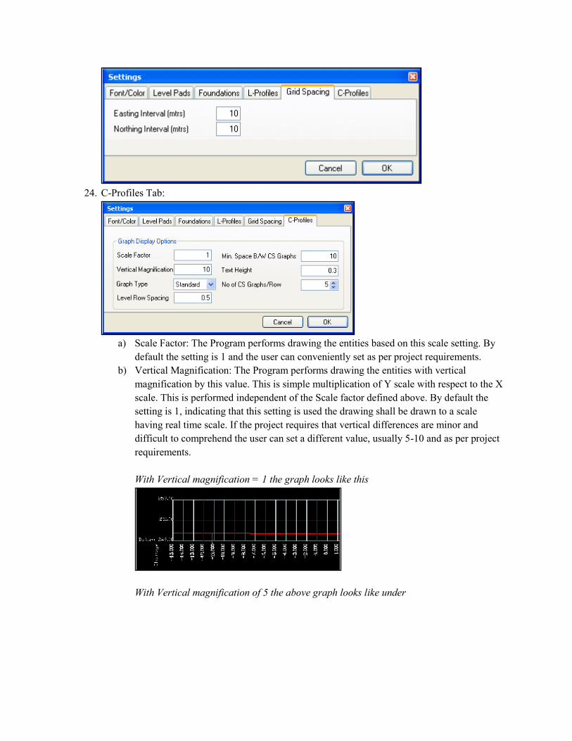
24. C-Profiles Tab:

a) Scale Factor: The Program performs drawing the entities based on this scale setting. By

default the setting is 1 and the user can conveniently set as per project requirements.

b) Vertical Magnification: The Program performs drawing the entities with vertical

magnification by this value. This is simple multiplication of Y scale with respect to the X

scale. This is performed independent of the Scale factor defined above. By default the

setting is 1, indicating that this setting is used the drawing shall be drawn to a scale

having real time scale. If the project requires that vertical differences are minor and

difficult to comprehend the user can set a different value, usually 5-10 and as per project

requirements.

With Vertical magnification = 1 the graph looks like this

With Vertical magnification of 5 the above graph looks like under

c) Level Row Spacing: Program writes/plots datum levels in graph at this spacing. For

example case we have the level intervals are 249, 250, 251 and so on at 1 meter intervals.

If we change this value to 2 meter intervals we will have 249, 251, 253 and so on.

d) Min. Space B/W CS Graphs: The Spacing between two Cross Sections. This setting plots

in either X or Y directions at the specified spacing.

e) Text height: Text height used in the entire graph shall have this value. User may change

as per the project requirements.

f) Nr of CS graphs/Row: Program plots this number of Cross Sections per row. For the

example case we have 5 plots in each row as shown in the output drawing file above.

Tutorial 7: Line Manipulations

Step 1: Tools >> Divide Polylines

25. We may need to develop cross sections along a path on a terrain or may need to have to do so

along set of 3D polylines already available from drawings. Division of polylines may be required

to indicate setting a fence object/array object along a polyline on those divided points. Or

creation of nodes as said above.

Step 2: Tools >> Join 3D lines:

26. AT times we may have 3D polylines available in our drawing in broken state and we may require

them to be joined for managing further. This feature would enable us to join the selected 3D

polylines, if contiguous, to make as single 3D polyline.

Step 3: Tools >> Convert Lines:

27. Sometimes we may be having some AutoCAD entities in different fashion than required for us.

In such places we may use the following commands to manipulate them as required.

e) Polyline to 3DPolyline:Here we can convert the polylines to 3Dpolyline

f) 3DPolyline to Polyline: Here we can convert the 3Dpolyline to polylines

g) Reverse 3DPolyline: Here we can the reverse the 3D polyline. Sometimes we need to

define a starting point of a project feature already drawn, but in reverse order.

h) Reverse Polyline: Here we can the reverse the polyline. Sometimes we need to define a

starting point of a project feature already drawn, but in reverse order.

Tutorial 8: Landscaping

Step 1: Edit Point Elevations: 28. This manipulations required to imply for inaccessible areas in project location, but can be

approximated by editing to give virtual effect.

29. You may need to edit some elevations for certain area where by approximation could only be

possible. Those area points shall be modified with random values or with a constant value. For

such creation of elevation changes we use the following dialog. Use menu command at Tools >>

Edit Point Elevations.

Set of Points before Editing the Elevation Set of Points after Editing the Elevation

aec terrain step by step tutorials 2: earthwork in area grading (level pads) step 1: follow step 1...

Documents