Advecting Procedural Textures for 2D Flow Animation

David Kao I and Alex Pang 2

1NASA Ames Research Center

2Computer Science Department, UCSC

Abstract

This paper proposes the use of specially generated 3D procedural textures for visualizing steady state

2D flow fields. We use the flow field to advect and animate the texture over time. _owever, using standard

texture advection techniques and arbitrary textures will introduce some undesirable effects such as: (a)

expanding texture from a critical source point, (b) streaking pattern from the boundary of the flow field,

(c) crowding of advected textures near an attracting spiral or sink, and (d) absent or lack of textures

in some re_ions of the flow. This paper proposes a number of strategies to solve these problems. We

demonstrate how the technique works using both synthetic data and computational fluid dynamics data.

Key Words and Phrases: Procedural textures, critical points, texture advection, animation, vector

field.

1 INTRODUCTION

It is hard to avoid staring at the dynamic motions of characters, objects, or almost anything else that

moves in an animated scene. Our attention span seems to last longer when watching a video than watch-

https://ntrs.nasa.gov/search.jsp?R=20020057891 2018-07-14T05:50:37+00:00Z

ing a set of static presentation slides. Recent advances in computer graphics and imaging research have

introduced many animation techniques that are based on flow advection [5, 7, 8]. These techniques allow

effective visualization of the flow trajectory by observing the movements and distortions of the textures.

However, most of them assume simple flow behaviors. In a computational fluid dynamics (CFD) simula-

tion, it is common to produce data sets with very complex flow patterns. Some of these include: saddles,

repelling nodes, repelling spirals, attracting nodes, attracting spirals, and centers (circular flows). Using

conventional texture advection techniques to animate these types flow may create undesirable artifacts.

A simple method for animating a 2D flow using texture advection can be described as follows: Con-

sider an input image and a velocity field defined over the image. Let n + 1 be the total number of time

steps in the animation, then for each time step ti, where i = 0,..., r_, advect every pixel backward from

time t, to to and save the morphed image Mi. To animate the flow, simply playback the saved images

Mi for all time steps. This texture advection method will work for most flow fields. However, when

there are repelling nodes or repelling spirals in the flow, then undesirable artifacts can be seen. In flow

topology, a repelling node is known as a critical point that generates a star-like outward flow pattern

while a repelling spiral is another type of critical point that generates an outward swirl flow pattern. For

both types of critical points, the flow would appear to be repelling away from the critical point during

flow animation. Hence, they are also known as source critical points.

Once the texture at a source critical point is advected, what texture should be used for the next advec-

tion at that critical point? Since the flow is being repelled away from the critical point, there is no new

texture available! With a texture advection method such as the one just described earlier, one would see

an expansion of the original texture color from the source critical point; thus, creating an undesirable ar-

tifacts. This artifact can also occur at the image border where there are incoming flows. Analogously, the

problem is that once the original texture at the border has been advected forward, what texture should be

used next at the border? Here the artifact is caused by an expansion of constant texture from the border.

Figure 1 shows a time sequence of animating 2D flows using the texture advection method described

2

above.The left imageshowstheinput textureimage. As we stepforward in time, we canseethearti-

factsgeneratedby thesourcecritical point located near the lower-right of the image. The constant bands

of texture from the upper-left border of the image are caused by the inflow from the border.

(a) Time Step 0 (b) Time Step 5 (c) Time Step 10 (d) Time Step 20

Figure 1. A time sequence of animating 2D flows using texture advection. Artifacts of constant texture

due to the source critical point located on the lower right portion of the image and the constant texture

bands from the upper left border due to inflow.

One may consider using periodic textures to feed in textures from the other side as soon as a backward

integrated streamline hits a boundary. However, the underlying cause of these artifacts can be attributed

to the absence of flow information to guide the texture selection. For the case of inflow from the border,

we do not have flow data to determine the next position of the streamline when it is integrated backwards.

Likewise, for a source critical point, the backward integrated streamline always arrive at the same point.

Hence, the artifact of expansion from a single texel. In our earlier work, we proposed an alternative

method to texture advection, based on streamline cycling, to alleviate these artifacts [3]. In this paper, we

introduce a technique for eliminating these artifacts using the more traditional texture advection method

and which provides a more continuous texture than the streamline cycling method. We also propose two

texture patterns that are ideal for animating 2D flow fields. Finally, we apply our techniques to two real

world flow data.

3

2 FLOWS FROM BOUNDARY

Assume that a steady state vector function 17(p) is defined for all position p in the image grid G and

t C [to, tn], where n 4- 1 is the total number of time steps in the animation. For texture advection, each

pixel in the image is considered as a massless particle. To create an animation, we integrate backwards

to determine where the particle at p might have come from. We then sequentially transfer the textures

over the path of the particle to p.

The path of particle at p can be computed by numerically integrating the vector function l,?(p). Since

we are dealing with steady flow fields, we can treat the animation time at ti as our integration time at

tk. That is, tk = ti. Let tk be the current time step, P0 be the initial particle position for each pixel,

and initially, k = 0, then the particle can be advected backwards from tk to to using a second-order

Runge-Kutta integration with:

K = -hP( )

K

tk+l = tk -- h and k = k + 1, (1)

where h is the integration step size and 0 < h < 1. The texture at P0 is then replaced by that at Pk to

generate an animation frame for time tk. We referred to the texture at Pk as the replacement texture. To

generate an animation sequence of morphed images that depict the flow described by V(p) the texture

advection algorithm is performed for all ti, where i = 0,..., n. At each time step, if the integration ends

prematurely, tk > to in Equation 1, then the particle has either reached the boundary or it has reached

a critical point, where the velocity is zero. Again, note that for the case of steady flow, we can freely

J

interchange tk and ti.

4

Supposethat theparticlehasreachedthegrid boundary,thentwo straightforwardmethodsto deter-

mine thereplacementtexturefor P0 are as follows: (1) let the replacement texture be that at Pk where

the integration ends; and (2) assume a periodic boundary condition such that the particle is wrapped

around to the "opposite" side of the boundary. Both methods will produce undesirable artifacts. The

first method would cause constant texture bands to flow into the image from the border, while the latter

would cause incoherent textures to feed into the image from the border.

Ideally, we want to have a continuous texture to feed from the boundaries of the grid as time pro-

gresses. We found that the most effective method is to define a 3D procedural texture function T(u, v, w)

and compute the replacement texture on the fly whenever the particle integration ends. In Section 4, we

will describe the texture function T in more detail. For now, we assume that the function T is given.

We determine the coordinates (u, v, w) of the 3D texture function based on the last position Pk where

the integration ends and on the current tk at the end of the integration. Let u = _M and v = p-_N, where

M and N are the image dimensions. If the particle integration ends prematurely, then we let w = _tn _

where t_ is the remaining number of time steps that were not integrated i.e. tr = tk - to. Otherwise,

we let w = 0 for all particle integrations that ends successfully. We can think of the texture function T

being defined in a unit cube and when the integration ends prematurely, we simply step into the cube

along the w axis by a depth of t_. Otherwise, we use T(u, v, O) as the replacement texture. Figure 2(a)

illustrates this method.

3 FLOWS FROM REPELLING NODES

Here we are interested in generating flow textures from source critical points such that the physical

flow behavior surrounding each critical point is clearly depicted. For this type of critical point, we want

new textures to flow out of the critical point. We propose two approaches to generate such flow textures.

The first approach is based on the method described in !he previous section for providing continuous

W

W //

Pk

(a) (b) (c)

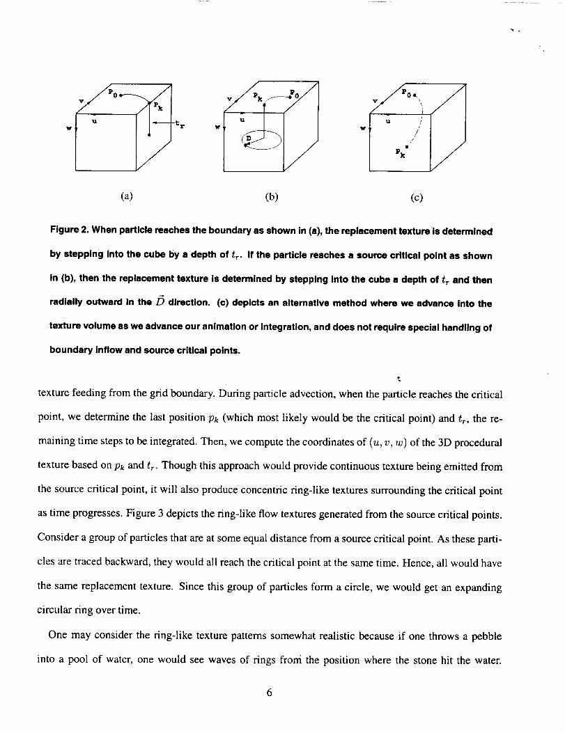
Figure 2. When particle reaches the boundary as shown in (a), the replacement textureis determined

by stepping into the cube by a depth of tr. If the particle reaches a source critical point as shown

in (b), then the replacement texture is determined by stepping Into the cube s depth of tr and then

radially outward in the V direction. (c) depicts an alternative method where we advance into the

texture volume as we advance our animation or integration, and does not require special handling of

boundary inflow and source critical points.

texture feeding from the grid boundary. During particle advection, when the particle reaches the critical

point, we determine the last position Pk (which most likely would be the critical point) and tr, the re-

maining time steps to be integrated. Then, we compute the coordinates of (u, v, w) of the 3D procedural

texture based on Pk and tr. Though this approach would provide continuous texture being emitted from

the source critical point, it will also produce concentric ring-like textures surrounding the critical point

as time progresses. Figure 3 depicts the ring-like flow textures generated from the source critical points.

Consider a group of particles that are at some equal distance from a source critical point. As these parti-

cles are traced backward, they would all reach the critical point at the same time. Hence, all would have

the same replacement texture. Since this group of particles form a circle, we would get an expanding

circular ring over time.

One may consider the ring-like texture patterns somewhat realistic because if one throws a pebble

into a pool of water, one would see waves of rings fiord the position where the stone hit the water.

(a)Time Step0 (b) Time Step5

(c) TimeStep10 (d) Time Step 20

Figure 3. Flow data with one source critical point on the lower right and a sink critical point on the

upper left. This time sequence depicts concentric ring-like texture patterns coming out of the source

critical point.

However, the texture pattern does not really give the impression of the flow direction from the source

critical points. Therefore, we propose another approach that achieves this effect. For the last position

Pk, where the particle terminated, we step into the cube by a depth of t,. and then radially outward in

the incoming direction of P0- Figure 2(b) illustrates this method. Let/9 denote the incoming direction

and/9 = _ then we let u = IPk_+ R*/9_I IPk_ + R*/_ulIIp0-p,.ll' ._t + n v = ._t + n , and u, = t_ where R is a predefined

tn '

constant. To keep the values of u and v between zero and one, we use the absolute value in the numerator

because /9 can be negative. With this approach, we were able to replace the ring-like effect on the

animation with flow textures that radially emanate from the source critical points. Figure 4 depicts the

results of this approach with R = 180.

(a) Time Step 0 (b) Time Step 5

(c) Time Step 10 (d) Time Step 20

Figure 4. Flow data with two attracting nodes on the upper half and two repelling nodes on the lower

half. This time sequence depicts flow textures emitting from the source critical points in the direction

of the flow. The replacement texture is computed based on the method illustrated in Figure 2(b).

4 PROCEDURAL TEXTURE DESIGN

There are several issues and parameters to consider in designing textures for flow visualization. Poorly

designed textures will create problems such as: (a) over-crowding of textural patterns particularly near

attraction basins, and (b) lack of textural patterns in high shear regions. These can be addressed by first

selecting a suitable spatial frequency of the textures to fit the complexity of the flow patterns. Over-

crowding and absent of textures can be fixed by aging older textures and constantly introducing new

textures. That is, we use 3D textures for 2D flow fields. Care must also be taken to balance the spatial

frequency of the textures versus the temporal frequency so that the appearance of the advected textures

does not alter the apparent speed of the flow.

We experimented with two types of solid textures. In both cases, the goal was to produce a cloud-like

texture such that when it is advected and distorted, it would produce a wispy and fuzzy appearance of

cloud being blown by wind. The first one is based on procedural textures as described in pages 155 and

I.

156 of [1]. This technique uses a turbulence function to produce random looking clusters of various

sizes and distributions. The texture value at any point can be quickly calculated on the fly and one does

not need to store the 3D texture. Examples using this texture can be seen in Figures 3 and 4. However,

one have little control over the distribution of the texture values, and in our application, may exacerbate

the problem of over-crowding or under-population of advected textures over time.

The second technique creates 3D textures by populating a volume with spheres. The parameters

include average size of the spheres, average distance between spheres, and how the texture varies within

a sphere. We use a poisson disk distribution to maintain a minimum average distance among the spheres.

For each sphere, we vary the texture value from 1.0 at the center to 0.5 at the surface. This helps produce

softer fuzzy spheres.

In generating the 3D textures, we note that one must take into account both spatial and temporal scales

of the flow data. That is, the patterns in the texture must nol; be too large so that it misses the flow pattern.

9

For example, if the texture consists of one very large sphere and the flow consist of numerous critical

points, then the advected texture will not be able to effectively reveal the nature of the flow. Likewise,

the patterns in the texture must not be too small so that it quickly disappears and fades without showing

the flow pattern. With regards to temporal scales, the patterns should not vary too slowly or they linger

around too long in the animation and create over-crowding of textures; neither should they vary too fast

or they become distractions that make the animation blink with very short lived flashes. Figure 5 depicts

a time-sequence from the animation of three rotating vortices. In the animation, we advance into the

texture volume as illustrated in Figure 2(c). In Figure 5(a), the undistorted spheres in the texture are

shown. In (b), we start to see the distortion of the spheres caused by two rotating vortices near the upper

right and lower left of the image. In (c), the texture distortions caused by central vortex is also apparent.

Finally, in (d), the effects of the three vortices on the texture are shown. In addition, there are two saddle

structures located near the upper left and lower right of the image.

Using the sphere texture volume, we found the the animation generated by advancing into the texturet

volume at each time step (Figure 2(c)) is more sensitive to the size and number of spheres in the volume.

We had to experiment with several sphere sizes to obtain an animation that effectively revealed the flow.

On the other hand, the frequency scales included in the solid textures based on turbulence functions

seemed to be more robust.

Currently, we generate our textures based on trial and error, and do not yet have a systematic nor

heuristic method for automatically determining the appropriate spatial and temporal scales given a flow

field. The scales obviously will depend on the magnitude and complexity of the flow, and we plan to

pursue an investigation on how to generate a flow dependent texture for animation.

10

(a) Time Step 0 (b) Time Step 5

(c) Time Step 16 (d) Time Step 45

Figure 5. Advection of 3D sphere textures using flow data with three rotating vortices located diago-

nally across the image.

11

5 RESULTS

We now describe some results of applying the proposed techniques on two CFD data sets. The first

data set is the first time step of a cross section of flow around an oscillating airfoil. A good background

description of the data can be found in [4, 6]. The second data set is surface flow information on a

hemisphere cylinder. Alternative ways of visualizing this data set can be found in [9, 2]

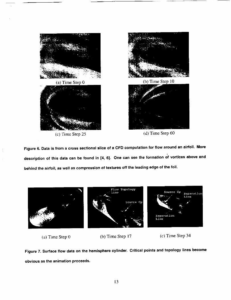
Figure 6 shows four frames of our flow animation using texture advection. In (a), we see the geometry

of the wing profile, how the procedural texture looks like before it is advected, and also the discontinuity

at the trailing tip of the wing due to the wrap around of the curvilinear grid and non-periodic textures.

In (b), we start to see the formation of a primary clockwise vortex above the airfoil, and a secondary

counter-clockwise vortex near the trailing tip of the wing. In (c), the primary vortex becomes more

prominent. At the same time, we start to see some compression of textures forming at the leading edge

of the wing. Finally, in (d), the primary vortex has separated from the airfoil and the compressed textures

at the leading edge have become even more prominent. These sequence are belt seen in an animation

which is available for download from www.cso.ucsc.odu/rosoareh/avisltoxflow2d.hlrnl.

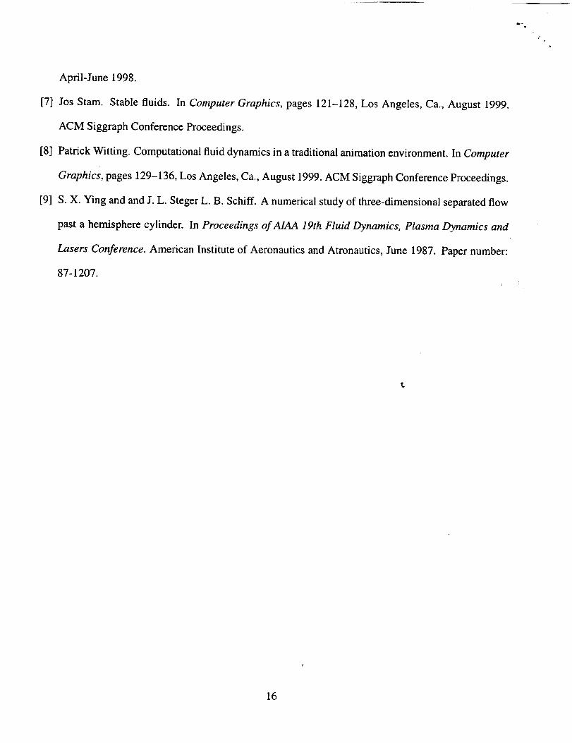
Figure 7 shows three views of three different time steps in our texture advection animation of the

surface flow on the hemisphere cylinder. In (a), we see the initial mapping of the un-advected textures

in the physical domain of the cylinder. In (b), we see a source critical point near the top of the surface.

Also, the sharp discontinuous curve running through most of the length of the cylinder correspond to

surface topology lines and indicates regions of flow with very different directions. In (c), the animation

has progressed further along and shows the persistence of certain flow patterns even though the textures

are dynamically being advected. Upon closer examination, one can see two separation lines along the

cylinder body. Note that there is also another critical point between the two separation lines. Further-

more, there is a source critical point near the nose of the cylinder. Again, these are best observed in an

animation which is available from the same web site mentioned above.

12

(a)TimeStep0 (b) TimeStep10

(c)Time Step25 (d)Time Step60

Figure 6. Data is from a cross sectional slice of a CFD computation for flow around an airfoil. More

description of this data can be found in [4, 6]. One can see the formation of vortices above and

behind the airfoil, as well as compression of textures off the leading edge of the foil.

(a) Time Step 0 (b) Time Step 17 (c) Time Step 34

Figure 7. Surface flow data on the hemisphere cylinder. Critical points and topology lines become

obvious as the animation proceeds.

13

When we first showed these texture animation of real flow data to our CFD scientists, they were very

surprised with seeing the animation. They have never seen this type of synthetic texture flow on their

flow data. Previously, they had mostly relied on the traditional streamline particle traces to observe their

flow trajectory. Almost all of them have very good comments about the animation and would like to see

our technique available to them soon.

6 CONCLUSION

We have described techniques and textures for animating 2D steady flow fields using texture advec-

tion. The method is straight forward and relatively easy to implement. The modifications introduced in

this paper also addressed all the difficulties identified in earlier texture advection work - over-crowding

and/or sparsity of textures over time, and handling of boundary inflow and repelling nodes. The paper

first demonstrated how the proposed methods and textures handled problematic cases using synthetic

flow data. We then applied it to two CFD data sets. Looking at still images in Figures 6 and 7, one can

already gain the benefit of this technique in the form of automatic extraction of flow features such as

location and type of critical points, as well as flow topology curves. These features and the flow pattern

in general are further accentuated when one views the animations.

There are a number of places for improvement and extension: (1) we think texture advection will be

most beneficial for unsteady flow data - this is what we observe in nature as clouds form and dissipate, or

as dyes swirl in a mixture; (2) the selection of the spatial and temporal scales of our textures is currently

by trial and error, we hope to come up with heuristics or recommendations for their selection based on

information about flow magnitudes; (3) the patterns coming out of source critical points may be either

concentric ring-like patterns as one might observe when a pebble is dropped in a pool, or it may be

appear like patterns shooting out of the source. When one is the mind-set of the latter case, we still

have a distracting ring pattern. We are exploring different ways of eliminating this extra ring; and (4)

14

\\

extension of this technique to steady and time varying 3D flow fields.

7 ACKNOWLEDGEMENTS

We would like to thank David Ebert for his suggestion on the ball textures, Chris Henze for his

program that generates arbitrary 2D flow fields, and Neal Chaderjian for his feedbacks on the texture

flow animation of the CFD data. The hemisphere cylinder data is courtesy of Susan Ying and the

airfoil data set is provided by Sungho Ko. We would also like to thank the members of the Advanced

Visualization and Interactive Systems laboratory at UC, Santa Cruz for their feedback and suggestions.

This project is supported in part by NASA grant NCC2-5281, LLNL Agreement No. B347879 under

DOE Contract No. W-7405-ENG-48, NSF NPACI ACI-9619020, and NSF ACI-9908881.

References

[1] David S. Ebert, F. Kenton Musgrave, Darwyn Peachey, Ken Perlin, and Stbven Worley. Texturing

and Modeling, A Procedural Approach. AP Professional, 1994.

[2] J. L. Helman and Lambertus Hesselink. Surface represenations of two and three-dimensional fluid

flow topology. In Proceedings: Visualization '90, pages 6-13. IEEE Computer Society, 1990.

[3] David Kao and Alex Pang. On animating 2D velocity fields. In SPIE Visual Data Exploration and

Analysis VIII, 2001. to appear.

[4] S. Ko and W. McCrosky. Computations of unsteady separating flows over an oscillating airfoil.

AIAA, 33rd Aerospace Sciences Meeting, January 1995. Paper number: 95-0312.

[5] N. Max, R. Crawfis, and D. Williams. Visualizing wind velocities by advecting cloud textures. In

Proceedings: Visualization '92, pages 179-184. IEEE Computer Society, 1992.

[6] Han-Wei Shen and David L. Kao. A new line integral convolution algorithm for visualizing time-

varying flow fields. IEEE Transactions on Visualization and Computer Graphics, 4(2):98-108,t

15

April-June 1998.

[7] JosStam. Stablefluids. In Computer Graphics, pages 121-128, Los Angeles, Ca., August 1999.

ACM Siggraph Conference Proceedings.

[8] Patrick Witting. Computational fluid dynamics in a traditional animation environment. In Computer

Graphics, pages 129-136, Los Angeles, Ca., August 1999. ACM Siggraph Conference Proceedings.

[9] S. X. Ying and and J. L. Steger L. B. Schiff. A numerical study of three-dimensional separated flow

past a hemisphere cylinder. In Proceedings of AIAA 19th Fluid Dynamics, Plasma Dynamics and

Lasers Conference. American Institute of Aeronautics and Atronautics, June 1987. Paper number:

87-1207.

_r

Je

16