Advantages and problems of soft computingBogdan M. Wilamowski

Auburn Universitywilam@ieee.org

Abstract - Soft computing can be a very attractive alternative to a purely digital system, but there are many traps waiting for researchers trying to apply this new exciting technology. For nonlinear processing both neural networks and fuzzy systems canbe used. Terrifically neural networks should provide much better solutions: smoother surfaces, larger number of inputs and outputs, better generalization abilities, faster processing time, etc. In industrial practice, however, many people are frustrated with neural networks not being aware that the reason for their frustrations are wrong learning algorithms and wrong neural network architectures. Having difficulties with neural network training, many industrial practitioner are enlarging neural networks and indeed such networks converges to solutions much faster. But at the same time such excessively large network are not able to respond correctly to new patterns which were not used for training. This paper describes how to use effective neural networks and how to avoid all reasons for frustration.

I. INTRODUCTION

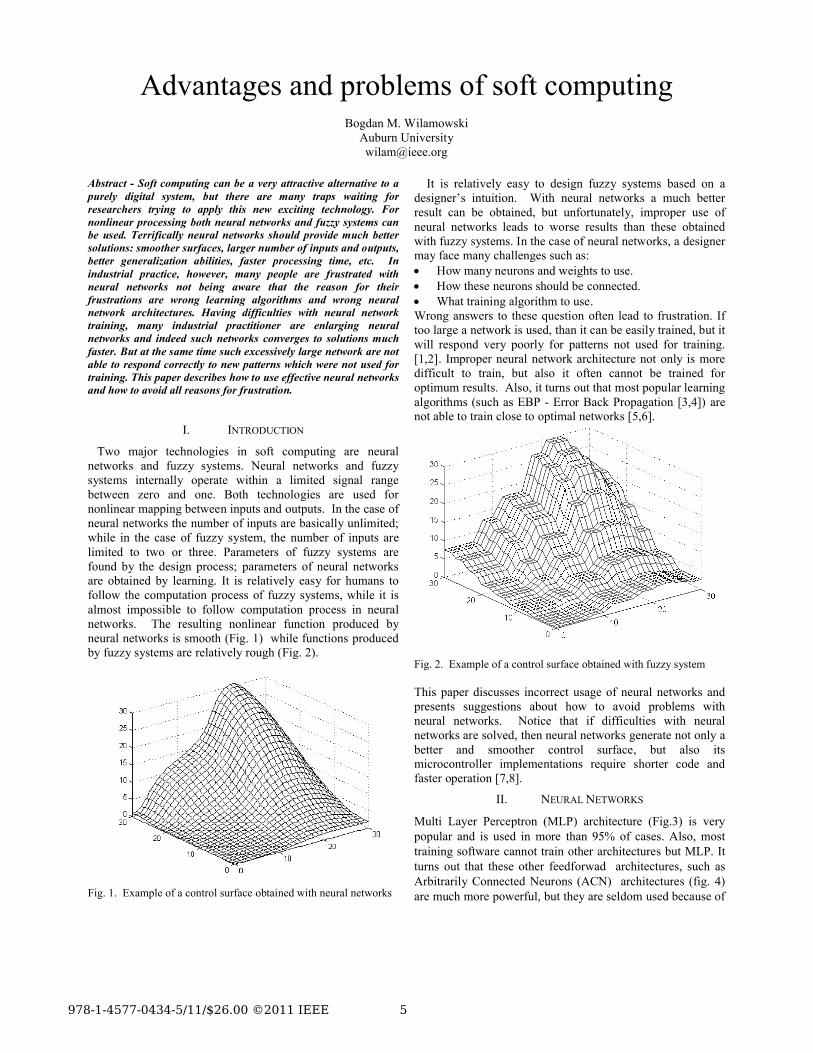
Two major technologies in soft computing are neural networks and fuzzy systems. Neural networks and fuzzy systems internally operate within a limited signal range between zero and one. Both technologies are used for nonlinear mapping between inputs and outputs. In the case of neural networks the number of inputs are basically unlimited;while in the case of fuzzy system, the number of inputs are limited to two or three. Parameters of fuzzy systems arefound by the design process; parameters of neural networks are obtained by learning. It is relatively easy for humans to follow the computation process of fuzzy systems, while it is almost impossible to follow computation process in neural networks. The resulting nonlinear function produced by neural networks is smooth (Fig. 1) while functions produced by fuzzy systems are relatively rough (Fig. 2).

Fig. 1. Example of a control surface obtained with neural networks

It is relatively easy to design fuzzy systems based on a designer’s intuition. With neural networks a much better result can be obtained, but unfortunately, improper use of neural networks leads to worse results than these obtained with fuzzy systems. In the case of neural networks, a designer may face many challenges such as: How many neurons and weights to use. How these neurons should be connected. What training algorithm to use.Wrong answers to these question often lead to frustration. If too large a network is used, than it can be easily trained, but it will respond very poorly for patterns not used for training. [1,2]. Improper neural network architecture not only is moredifficult to train, but also it often cannot be trained for optimum results. Also, it turns out that most popular learning algorithms (such as EBP - Error Back Propagation [3,4]) arenot able to train close to optimal networks [5,6].

Fig. 2. Example of a control surface obtained with fuzzy system

This paper discusses incorrect usage of neural networks and presents suggestions about how to avoid problems with neural networks. Notice that if difficulties with neural networks are solved, then neural networks generate not only a better and smoother control surface, but also its microcontroller implementations require shorter code and faster operation [7,8].

II. NEURAL NETWORKS

Multi Layer Perceptron (MLP) architecture (Fig.3) is very popular and is used in more than 95% of cases. Also, most training software cannot train other architectures but MLP. It turns out that these other feedforwad architectures, such as Arbitrarily Connected Neurons (ACN) architectures (fig. 4) are much more powerful, but they are seldom used because of

978-1-4577-0434-5/11/$26.00 ©2011 IEEE 5

lack of proper learning tools [9]. In feedforward networks one directional signal flow is assured. Neurons are connected by weights with different positive and negative values, and the resulting neuron excitation net is calculated as a sum ofproducts of incoming signals multiplied by weights:

xw=net ii

n

=1i (1)

Then, signals are passing through neurons' activation functions, which can be unipolar (Fig. 5.a) or bipolar (Fig. 5.b), and this leads to the question which type of activation functions to use: unipolar or bipolar? The short answer is that it does not matter.

Fig. 3. Multilayer Perceptron (MLP) type architecture 5-4-4-1

Fig. 4. Arbitrarily Connected Neurons (ACN) type architecture 3=1=2=2=1

Both types of networks work the same way, and it is very easy to transform bipolar a neural network into a unipolar neural network and vice versa. Moreover, there is no need to change most weights, but only the biasing weight has to be changed.

k

netknetfo uni

exp1

1)(

ookof uni 1)('

)(netf

net

(a)

k

2tanh1

exp1

21)(2)(

netk

netk

netfnetfo unibip

2

1)('

2okof bip

)(netf

net

(b)Fig. 5. Typical soft activation function of neurons (a) unipolar, (b) bipolar

In order to change from bipolar networks to unipolar networks, only biasing weights must be modified using the formula:

N

i

bipi

bipbias

unibias www

1

5.0 (6)

While in order to change from unipolar networks to bipolar networks :

N

i

unii

unibias

bipbias www

1

2 (7)

Fig. 6 shows the neural network for a parity-3 problem which can be transformed both ways: from bipolar to unipolar and from unipolar to bipolar. Notice that only biasing weights are different. Obviously input signals in the bipolar network should be in the range from -1 to +1 while for a unipolar network they should be in the range from 0 to +1.

-2

0

+1

weights 1

0bipolar

Fig. 6 Neural networks for parity-3 problem.

6

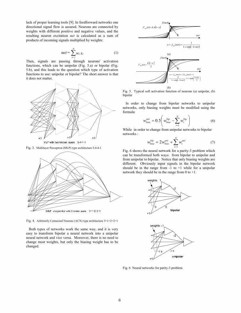
The strength of the neural network strongly depends on the used architecture. For example, Table I shows a minimum number of neurons required to solve popular Parity-N benchmarks with different values of N. Please notice that in order to solve a Parity-64 problem using the most popular MLP architecture with one hidden layer, 65 neurons arerequired. When a FCC (Fully Connected Cascade) architecture is used, then only 7 neurons are required to solve the same problem. One may question why researchers are using MLP instead of FCC architectures. A simple answer is that they know how to train MLP networks, but they do not know how to train FCC networks.

TABLE IMINIMUM NUMBER OF NEURONS REQUIRED TO SOLVE VARIOUS PARITY-N

PROBLEMS

Parity-8 Parity-16 Parity-32 Parity-64# inputs 8 16 32 64# patterns 256 65536 4.294e+9 1.845e+19MLP (one hidden layer)

98-8-1

1716-16-1

3332--32-1

6564-64-1

BMLP (one hidden layer)

58=4=1

916=8=1

1732=16=1

3364=32=1

BMLP (2hidden layer)

48=2=1=1

516=2=2=1

732=3=3=1

1163=5=5=1

BMLP (3hidden layer)

48=1=1=1=1

516=2=1=1=1

632=2=2=1=1

864=3=2=2=1

FCC 48=1=1=1=1

5 6 7

The most common training algorithm is EBP – Error Back Propagation [3,4]. It is relatively simple, and it does not require a lot of computer resources. This algorithm, however,seldom leads to a good solution and is extremely slow. Much better results can be obtained with the LM –Levenberg-Marquardt Algorithm [10,11], but even the LM algorithm cannot train other architectures but MLP. These more powerful neural network architectures can be efficiently trained by the recently developed Neuron by Neuron (NBN) learning algorithm [12-15]. The Neuron by Neuron (NBN) algorithm was developed

in order to eliminate most disadvantages of the LM algorithm. It can be used to train neural networks with arbitrarily connected neurons. It does not require to compute and to store large Jacobians, so it can train problems with basically unlimited number of patterns [14]. Error derivatives are computed only in the forward pass, so the backpropagation process is not needed [15]. It is equally fast, but in the case of networks with multiple outputs faster than LM algorithm. It canof course train networks which are impossible to train with other algorithms. Fig 7 shows training errors as a function of a number of interactions using popular EBP algorithm for Parity-4 problem using MLP architecture 4-3-3-1 (Fig. 7.a) and FCC architecture 4=1=1=1 (Fig. 7.b) [16]. For MLP network with 7 neurons, the EBP algorithm was successful in 50 % cases (Fig. 7.a); while the EBP algorithm failed for the FCC architecture network with 3 neurons, the EBP has failed on all tries(Fig.7.b).

(a)

(b)Fig. 7. Result of parity-4 training using EBP algorithm architecture: (a) with 4-3-3-1 architecture and success rate 50% and (b) with 4=1=1=1 architecture and success rate 0%. Average training times are 3797ms and 6223 ms respectively.

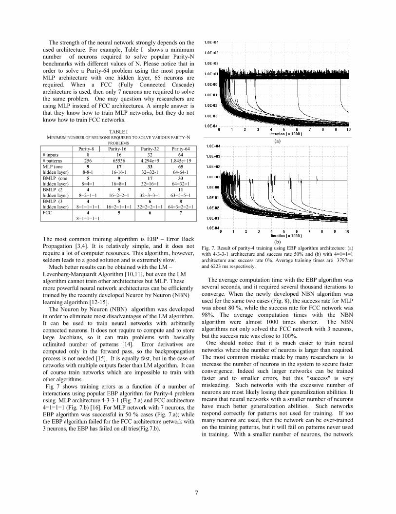
The average computation time with the EBP algorithm was several seconds, and it required several thousand iterations to converge. When the newly developed NBN algorithm was used for the same two cases (Fig. 8), the success rate for MLP was about 80 %, while the success rate for FCC network was 98%. The average computation times with the NBN algorithm were almost 1000 times shorter. The NBN algorithms not only solved the FCC network with 3 neurons,but the success rate was close to 100%. One should notice that it is much easier to train neural networks where the number of neurons is larger than required. The most common mistake made by many researchers is to increase the number of neurons in the system to secure faster convergence. Indeed such larger networks can be trained faster and to smaller errors, but this "success" is very misleading. Such networks with the excessive number of neurons are most likely losing their generalization abilities. It means that neural networks with a smaller number of neurons have much better generalization abilities. Such networksrespond correctly for patterns not used for training. If too many neurons are used, then the network can be over-trained on the training patterns, but it will fail on patterns never used in training. With a smaller number of neurons, the network

7

cannot be trained for very small errors, but it may produce much better approximations for new patterns.

(a)

(b)Fig. 8. Result of parity-4 training using NBN algorithm architecture: (a) with 4-3-3-1 architecture and success rate 80% and (b) with 4=1=1=1 architecture and success rate 98%. Average training times are 34 ms and 19 ms respectively.

0 1 2 3 4 5 6 7 8-2

-1.5

-1

-0.5

0

0.5

1

1.5

2

2.5

3

Fig. 9 Approximation of measured points by polynomials with a different orders stating with first through 9-th order.

The problem is similar to curve fitting using polynomial interpolation as illustrated in Fig. 9. Notice that if the order of polynomial is too low there is poor approximation everywhere. When the order is too high, there is a perfect fit at the given data points, but the interpolation between points is rather poor.

In the case of neural networks, we have a similar situation with an excessive number of neurons it is easy to train the network to a very small error at the training data, but this may lead to very poor and frustrating results when this trained neural network is used for process new patterns.

-10-5

05

10

-10

-5

0

5

10

-10

-5

0

5

10

Fig. 10. Control surface of TSK fuzzy controller with 8*6=48 defuzzyfication rules

-10

-5

0

5

10-10

-50

510

-10

-5

0

5

10

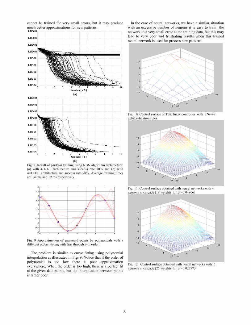
Fig. 11 Control surface obtained with neural networks with 4 neurons in cascade (18 weights) Error=0.049061

-10

-5

0

5

10-10

-50

510

-10

-5

0

5

10

Fig. 12 Control surface obtained with neural networks with 5 neurons in cascade (25 weights) Error=0.023973

8

In order to have good generalization abilities, the number of neurons in the network should be as small as possible to obtain a reasonable training error. The generalization abilities also depend on the number of training patterns. With a large number of training patterns, a larger number of neurons can be used while generalization abilities are preserved. To illustrate the problem with neural networks, let us try to find the best neural network architecture to replace a fuzzy controller. Fig. 10 shows the required control surface and the defuzzyfication rules for the TSK (Takagi-Sugeno-Ken) fuzzy controller [5,9]. In order to train the developed neural controller, we may use TSK defuzzyfication rules as the training patterns. Let us select the FCC neural networks architecture and try to find solutions for different number of neurons used. Fig. 11 shows results for 4 neurons and 18 weights. Fig. 12 shows results for the network with 5 neurons and 25 weights. When the size of the network increased, the results become worse instead of better despite that learning errors decrease with the increase of the neural network size.

III. FUZZY SYSTEMS

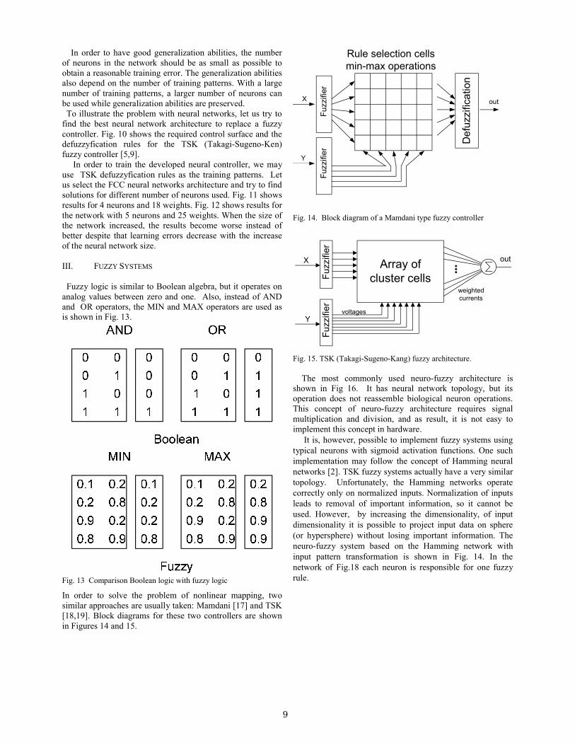
Fuzzy logic is similar to Boolean algebra, but it operates on analog values between zero and one. Also, instead of AND and OR operators, the MIN and MAX operators are used as is shown in Fig. 13.

Fig. 13 Comparison Boolean logic with fuzzy logic

In order to solve the problem of nonlinear mapping, two similar approaches are usually taken: Mamdani [17] and TSK[18,19]. Block diagrams for these two controllers are shown in Figures 14 and 15.

Fu

zzifi

er

X

Y

out

De

fuzz

ifica

tion

Fuz

zifie

r

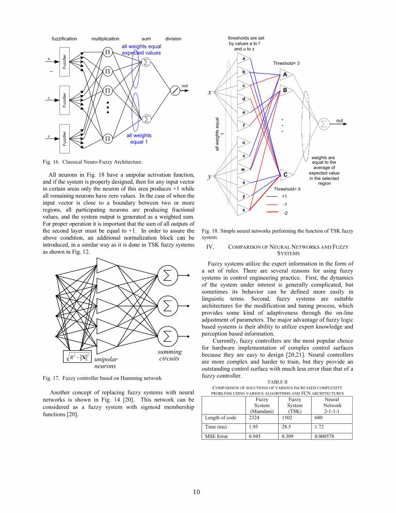
Rule selection cellsmin-max operations

Fig. 14. Block diagram of a Mamdani type fuzzy controller

Fuz

zifie

rF

uzzi

fier

X

Y

Array of cluster cells

out

weightedcurrents

voltages

Fig. 15. TSK (Takagi-Sugeno-Kang) fuzzy architecture.

The most commonly used neuro-fuzzy architecture is shown in Fig 16. It has neural network topology, but its operation does not reassemble biological neuron operations. This concept of neuro-fuzzy architecture requires signal multiplication and division, and as result, it is not easy to implement this concept in hardware. It is, however, possible to implement fuzzy systems using typical neurons with sigmoid activation functions. One such implementation may follow the concept of Hamming neural networks [2]. TSK fuzzy systems actually have a very similar topology. Unfortunately, the Hamming networks operate correctly only on normalized inputs. Normalization of inputs leads to removal of important information, so it cannot be used. However, by increasing the dimensionality, of input dimensionality it is possible to project input data on sphere (or hypersphere) without losing important information. The neuro-fuzzy system based on the Hamming network with input pattern transformation is shown in Fig. 14. In the network of Fig.18 each neuron is responsible for one fuzzy rule.

9

out

multiplication

Fu

zzifi

er

X

Fu

zzifi

er

y

Fu

zzifi

er

z

sumfuzzification division

all weights equal 1

all weights equal expected values

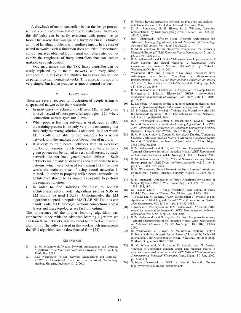
Fig. 16. Classical Neuro-Fuzzy Architecture.

All neurons in Fig. 18 have a unipolar activation function,and if the system is properly designed, then for any input vector in certain areas only the neuron of this area produces +1 while all remaining neurons have zero values. In the case of when the input vector is close to a boundary between two or more regions, all participating neurons are producing fractional values, and the system output is generated as a weighted sum.For proper operation it is important that the sum of all outputs of the second layer must be equal to +1. In order to assure theabove condition, an additional normalization block can be introduced, in a similar way as it is done in TSK fuzzy systemsas shown in Fig. 12.

unipolarneurons

summingcircuits

22 XR

Fig. 17. Fuzzy controller based on Hamming network

Another concept of replacing fuzzy systems with neural networks is shown in Fig. 14 [20]. This network can be considered as a fuzzy system with sigmoid membership functions [20].

x

y

allw

eig

hts

equ

al1

weights areequal to theaverage of

expected valuein the selected

region

Threshold= 3

thresholds are setby values a to f

and u to z

A

B

Cw

e

d

f

c

b

a

x

y

z

u

v

+1

-1

out

-2

Threshold= 5

Fig. 18. Simple neural networks performing the function of TSK fuzzy system.

IV. COMPARISON OF NEURAL NETWORKS AND FUZZY SYSTEMS

Fuzzy systems utilize the expert information in the form of a set of rules. There are several reasons for using fuzzy systems in control engineering practice. First, the dynamics of the system under interest is generally complicated, but sometimes its behavior can be defined more easily in linguistic terms. Second, fuzzy systems are suitable architectures for the modification and tuning process, which provides some kind of adaptiveness through the on-line adjustment of parameters. The major advantage of fuzzy logic based systems is their ability to utilize expert knowledge and perception based information.

Currently, fuzzy controllers are the most popular choice for hardware implementation of complex control surfaces because they are easy to design [20,21]. Neural controllers are more complex and harder to train, but they provide an outstanding control surface with much less error than that of a fuzzy controller.

TABLE IICOMPARISON OF SOLUTIONS OF VARIOUS INCREASED COMPLEXITY

PROBLEMS USING VARIOUS ALGORITHMS AND FCN ARCHITECTURES

FuzzySystem

(Mamdani)

FuzzySystem(TSK)

NeuralNetwork2-1-1-1

Length of code 2324 1502 680

Time (ms) 1.95 28.5 1.72

MSE Error 0.945 0.309 0.000578

10

A drawback of neural controllers is that the design process is more complicated than that of fuzzy controllers. However, this difficulty can be easily overcome with proper design tools. One severe disadvantage of a fuzzy system is its limited ability of handling problems with multiple inputs. In the case of neural networks, such a limitation does not exist. Furthermore, control surfaces obtained from neural controllers also do not exhibit the roughness of fuzzy controllers that can lead to unstable or rough control.

One may notice that the TSK fuzzy controller can be easily replaced by a neural network with very simple architecture. In this case the intuitive fuzzy rules can be used as patterns to train neural networks. This approach is not only very simple, but it also produces a smooth control surface.

V. CONCLUSION

There are several reasons for frustration of people trying to adapt neural networks for their research: In most cases the relatively inefficient MLP architecture

is used instead of more powerful topologies [22] where connections across layers are allowed.

When popular learning software is used, such as EBP, the training process is not only very time consuming, but frequently the wrong solution is obtained. In other words EBP is often not able to find solutions for a neural network with the smallest possible number of neurons

It is easy to train neural networks with an excessive number of neurons. Such complex architectures for a given pattern can be trained to very small errors, but such networks do not have generalization abilities. Such networks are not able to deliver a correct response to new patterns, which were not used for training [1][9]. In other words the main purpose of using neural networks is missed. In order to properly utilize neural networks, its architecture should be as simple as possible to perform the required function.

In order to find solutions for close to optimal architectures, second order algorithms such as NBN or LM should be used [13,23] Unfortunately, the LM algorithm adopted in popular MATLAB NN Toolbox can handle only MLP topology without connections across layers and these topologies are far from optimal.

The importance of the proper learning algorithm was emphasized since with the advanced learning algorithm we can train those networks, which cannot be trained with simple algorithms. The software used in this work which implements the NBN algorithm can be downloaded from [24].

REFERENCES

[1] B. M. Wilamowski, "Neural Network Architectures and Learning Algorithms," IEEE Industrial Electronics Magazine, vol. 3, no. 4, pp. 56-63, Dec. 2009

[2] B.M. Wilamowski “Neural Network Architectures and Learning”, ICIT'03 - International Conference on Industrial Technology, Maribor, Slovenia, December 10-12, 2003

[3] P. Werbos, Beyond regression: new tools for prediction and analysis in behavioral sciences. Ph.D. diss., Harvard University, 1974.

[4] D. E Rumelhart., G. E. Hinton, R. J. Williams, “Learning representations by back-propagating errors”. Nature, vol. 323, pp. 533-536, 1986.

[5] B.M. Wilamowski “Efficient Neural Network Architectures and Advanced Training Algorithms”, Gdańsk University of Technology Faculty of ETI Annals, Vol 18, pp. 345-352, 2010

[6] B. M. Wilamowski, H. Yu, “Improved Computation for Levenberg Marquardt Training,” IEEE Trans. on Neural Networks, vol. 21, no. 6, pp. 930-937, June 2010.

[7] B. M Wilamowski and J. Binfet " Microprocessor Implementation of Fuzzy Systems and Neural Networks ", International Joint Conference on Neural Networks (IJCNN'01), pp. 234-239,Washington DC, July 15-19, 2001

[8] Wilamowski B.M. and J. Binfet, " Do Fuzzy Controllers Have Advantages over Neural Controllers in Microprocessor Implementation" Proc of.2-nd International Conference on Recent Advances in Mechatronics - ICRAM'99, Istanbul, Turkey, pp. 342-347, May 24-26, 1999

[9] B. M. Wilamowski, " Challenges in Applications of Computational Intelligence in Industrial Electronics" ISIE10 - International Symposium on Industrial Electronics, Bari, Italy, July 4-7, 2010,pp. 15-22.

[10] K. Levenberg, “A method for the solution of certain problems in least squares”. Quarterly of Applied Machematics, 5, pp. 164-168, 1944.

[11] M. T. Hagan, and M. Menhaj, “Training feedforward networks with the Marquardt algorithm”, IEEE Transactions on Neural Networks, vol. 5, no. 6, pp. 989-993, 1994

[12] B. M. Wilamowski, N. Cotton, J. Hewlett, and O. Kaynak, “Neural Network Trainer with Second Order Learning Algorithms”, 11th INES 2007 -International Conference on Intelligent Engineering Systems,Budapest, Hungary, June 29 2007-July 1 2007, pp. 127-132

[13] B. M. Wilamowski, N. J. Cotton, O. Kaynak, G. Dundar, "Computing Gradient Vector and Jacobian Matrix in Arbitrarily Connected Neural Networks," IEEE Trans. on Industrial Electronics, vol. 55, no. 10, pp. 3784-3790, Oct 2008

[14] B. M. Wilamowski and O. Kaynak, "Oil Well Diagnosis by sensing Terminal Characteristics of the Induction Motor," IEEE Transactions on Industrial Electronics, Vol 47, No 5, pp. 1100-1107, October 2000.

[15] B. M. Wilamowski and H. Yu, “Neural Network Learning Without Backpropagation," IEEE Trans. on Neural Networks, vol. 21, no.11, pp. 1793 - 1803 Nov. 2010.

[16] B. M. Wilamowski, “Neural Networks or Fuzzy Systems” Workshop on Intelligent Systems, Budapest, Hungary, August 30, 2009, pp. 1-12.

[17] E. H. Mamdani, “Application of Fuzzy Algorithms for Control of Simple Dynamic Plant,” IEEE Proceedings, Vol. 121, No. 12, pp. 1585-1588, 1974.

[18] M. Sugeno and G. T. Kang, “Structure Identification of Fuzzy Model,” Fuzzy Sets and Systems, Vol. 28, No. 1, pp. 15-33, 1988.

[19] T. Takagi and M. Sugeno, “Fuzzy Identification of Systems and Its Application to Modeling and Control,” IEEE Transactions on System, Man, Cybernetics, Vol. 15, No. 1, pp. 116-132, 1985.

[20] J. Kolbusz, S. Paszczyński and B.M. Wilamowski, “Network traffic model for industrial environment”, IEEE Transaction on Industrial Informatics, vol. 2, No. 4, pp. 213-220, 2006.

[21] B. M. Wilamowski and O. Kaynak, "Oil Well Diagnosis by sensing Terminal Characteristics of the Induction Motor," IEEE Transactions on Industrial Electronics, Vol 47, No 5, pp. 1100-1107, October 2000.

[22] B. Wilamowski, D. Hunter, A. Malinowski, "Solving Parity-n Problems with Feedforward Neural Network," Proc. of the IJCNN'03 International Joint Conference on Neural Networks, pp. 2546-2551, Portland, Oregon, July 20-23, 2003

[23] B. M. Wilamowski, N. J. Cotton, O. Kaynak,, and G. Dundar, “Method of computing gradient vector and Jacobian matrix in arbitrarily connected neural networks” ISIE 2007- IEEE International Symposium on Industrial Electronics, Vigo, Spain, 4-7 June 2007, pp. 3298-3303

[24] Software Download - NNT - Neural Network Trainer http://www.eng.auburn.edu/~wilambm/nnt/.

11