advanced section #1: linear algebra and hypothesis testing · advanced section 1 today’s topics:...

CS109A Introduction to Data SciencePavlos Protopapas and Kevin Rader

Advanced Section #1: Linear Algebra and Hypothesis Testing

1

Will Claybaugh

CS109A, PROTOPAPAS, RADER

Advanced Section 1

WARNING

This deck uses animations to focus attention and break apart complex concepts.

Either watch the section video or read the deck in Slide Show mode.

2


Advanced Section 1

Today’s topics:

Linear Algebra (Math 21b, 8 weeks)

Maximum Likelihood Estimation (Stat 111/211, 4 weeks)

Hypothesis Testing (Stat 111/211, 4 weeks)

Our time limit: 90 minutes

3

• We’ll work together

• I owe you this knowledge

• Come debt collect at OHs if I don’t do my job today

• Let’s do this : )

• We will move fast

• You are only expected to catch the big ideas

• Much of the deck is intended as notes

• I will give you the TL;DR of each slide

• We will recap the big ideas at the end of each section

LINEAR ALGEBRA

4

(THE HIGHLIGHTS)


Interpreting the dot product

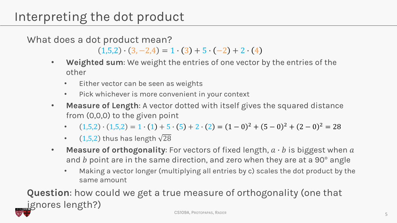
What does a dot product mean?1,5,2 % 3, −2,4 = 1 % 3 + 5 % −2 + 2 % 4

• Weighted sum: We weight the entries of one vector by the entries of the other• Either vector can be seen as weights

• Pick whichever is more convenient in your context

• Measure of Length: A vector dotted with itself gives the squared distance from (0,0,0) to the given point• 1,5,2 % 1,5,2 = 1 % 1 + 5 % 5 + 2 % 2 = 1 − 0 , + 5 − 0 , + 2 − 0 , = 28• 1,5,2 thus has length 28�

• Measure of orthogonality: For vectors of fixed length, 𝑎 % 𝑏 is biggest when 𝑎and 𝑏 point are in the same direction, and zero when they are at a 90° angle• Making a vector longer (multiplying all entries by c) scales the dot product by the

same amount

Question: how could we get a true measure of orthogonality (one that ignores length?)

5


Dot Product for Matrices

Matrix multiplication is a bunch of dot products• In fact, it is every possible dot product, nicely organized

• Matrices being multiplied must have the shapes 𝑛,𝑚 % 𝑚, 𝑝 and the result is of size 𝑛, 𝑝• (the middle dimensions have to match, and then drop out)

6

2 -1 3

1 5 2

-1 1 3

6 4 9

2 2 1

3 1

-2 7

4 -2

20 -11

1 32

7 0

46 16

6 14

% =2,2,1 % 1,7, −2

1 5 23

-2

4

11,5,2 % 3, −2,4

5 by 3

3 by 2

5 by 2


-1

5

1

4

2

Column by Column

• Since matrix multiplication is a dot product, we can think of it as a weighted sum• We weight each column as specified, and sum them together

• This produces the first column of the output

• The second column of the output combines the same columns under different weights

• Rows?7

2 -1 3

1 5 2

-1 1 3

6 4 9

2 2 1

3

-2

4

20

1

7

46

6

% =3

2

3

9

1

4+ =%-2 %

2

1

-1

6

2

3 % +

2 -1 3

1 5 2

-1 1 3

6 4 9

2 2 1

3 1

-2 7

4 -2

20 -11

1 32

7 0

46 16

6 14


3 1

-2 7

4 -2

Row by Row

• Apply a row of A as weights on the rows B to get a row of output

8

1 5 2 % = =

1 %

+

3 1

5 %

+

-2 7

2 % 4 -2

1 32

2 -1 3

1 5 2

-1 1 3

6 4 9

2 2 1

3 1

-2 7

4 -2

20 -11

1 32

7 0

46 16

6 14

LINEAR ALGEBRASpan

9

(THE HIGHLIGHTS)


𝛽7𝛽,

Span and Column Space

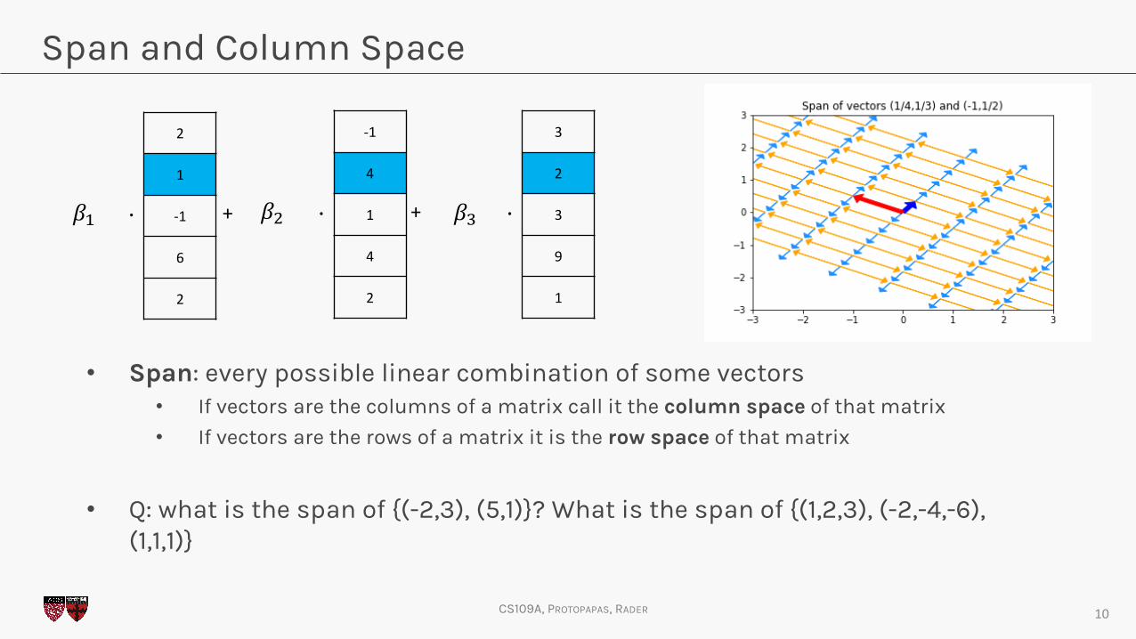
• Span: every possible linear combination of some vectors• If vectors are the columns of a matrix call it the column space of that matrix

• If vectors are the rows of a matrix it is the row space of that matrix

• Q: what is the span of {(-2,3), (5,1)}? What is the span of {(1,2,3), (-2,-4,-6), (1,1,1)}

10

-1

4

1

4

2

3

2

3

9

1

+ %%

2

1

-1

6

2

𝛽8 % +

LINEAR ALGEBRABases

11

(THE HIGHLIGHTS)


Basis Basics

• Given a space, we’ll often want to come up with a set of vectors that span it

• If we give a minimal set of vectors, we’ve found a basis for that space

• A basis is a coordinate system for a space• Any element in the space is a weighted sum of the basis elements

• Each element has exactly one representation in the basis

• The same space can be viewed in any number of bases - pick a good one 12


Function Bases• Bases can be quite abstract:

• Taylor polynomials express any analytic function in the infinite basis 1, 𝑥, 𝑥,, 𝑥7, …

• The Fourier transform expresses many functions in a basis built on sines and cosines

• Radial Basis Functions express functions in yet another basis

• In all cases, we get an ‘address’ for a particular function• In the Taylor basis, sin(𝑥) =

(0,1,0, 8A, 0, 8

8,B, … )

• Bases become super important in feature engineering• Y may depend on some transformation of x,

but we only have x itself

• We can include features 1, 𝑥, 𝑥,, 𝑥7, … to approximate

13

Taylor approximations to y=sin(x)

LINEAR ALGEBRAInterpretingTransposeandInverse

14

(THE HIGHLIGHTS)


3 1

2 -1

3 2

9 7

Transpose

• Transposes switch columns and rows. Written 𝐴D

• Better dot product notation: 𝑎 % 𝑏 is often expressed as 𝑎D𝑏• Interpreting: The matrix multiplilcation 𝐴𝐵 is rows of A dotted with columns of B

• 𝐴D𝐵 is columns of 𝐴 dotted with columns of 𝐵• 𝐴𝐵D is rows of 𝐴 dotted with rows of 𝐵

• Transposes (sort of) distribute over multiplication and addition:

𝐴𝐵 D = 𝐵D𝐴D 𝐴 + 𝐵 D = 𝐴D + 𝐵D 𝐴D D = 𝐴

15

3

2

3

9

3 2 3 9𝑥 = 𝑥D =3 2 3 9

1 -1 2 7𝐴 = 𝐴D =


Inverses

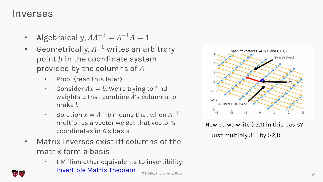
• Algebraically, 𝐴𝐴F8 = 𝐴F8𝐴 = 1• Geometrically, 𝐴F8 writes an arbitrary

point 𝑏 in the coordinate system provided by the columns of 𝐴• Proof (read this later):

• Consider 𝐴𝑥 = 𝑏. We’re trying to find weights 𝑥 that combine 𝐴’s columns to make 𝑏

• Solution 𝑥 = 𝐴F8𝑏 means that when 𝐴F8multiplies a vector we get that vector’s coordinates in A’s basis

• Matrix inverses exist iff columns of the matrix form a basis• 1 Million other equivalents to invertibility:

Invertible Matrix Theorem16

How do we write (-2,1) in this basis?

Just multiply 𝐴F8 by(-2,1)

LINEAR ALGEBRAEigenvaluesandEigenvectors

17

(THE HIGHLIGHTS)


Eigenvalues

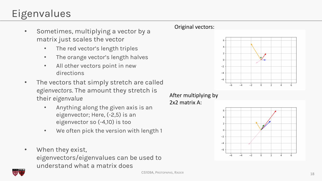
• Sometimes, multiplying a vector by a matrix just scales the vector• The red vector’s length triples

• The orange vector’s length halves

• All other vectors point in new directions

• The vectors that simply stretch are called egienvectors. The amount they stretch is their eigenvalue• Anything along the given axis is an

eigenvector; Here, (-2,5) is an eigenvector so (-4,10) is too

• We often pick the version with length 1

• When they exist, eigenvectors/eigenvalues can be used to understand what a matrix does

18

Originalvectors:

Aftermultiplyingby2x2matrixA:


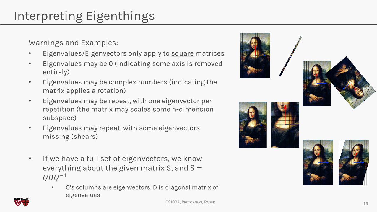
Interpreting Eigenthings

Warnings and Examples:• Eigenvalues/Eigenvectors only apply to square matrices

• Eigenvalues may be 0 (indicating some axis is removed entirely)

• Eigenvalues may be complex numbers (indicating the matrix applies a rotation)

• Eigenvalues may be repeat, with one eigenvector per repetition (the matrix may scales some n-dimension subspace)

• Eigenvalues may repeat, with some eigenvectors missing (shears)

• If we have a full set of eigenvectors, we know everything about the given matrix S, and S =𝑄𝐷𝑄F8• Q’s columns are eigenvectors, D is diagonal matrix of

eigenvalues

• Question: how can we interpret this equation?

19


Calculating Eigenvalues

• Eigenvalues can be found by:• A computer program

• But what if we need to do it on a blackboard?• The definition 𝐴𝑥 = 𝜆𝑥

• This says that for special vectors x, multiplying by the matrix A is the same as just scaling by 𝜆 (x is then an eigenvector matching eigenvalue 𝜆)

• The equation det 𝐴 − 𝜆𝐼O = 0• 𝐼O is the n by n identity matrix of size n by

n. In effect, we subtract lambda from the diagonal of A

• Determinants are tedious to write out, but this produces a polynomial in 𝜆 which can be solved to find eigenvalues

20

• Eigenvectors matching known eigenvalues can be found by solving A − 𝜆𝐼O 𝑥 =0 for x

LINEAR ALGEBRAMatrixDecomposition

21

(THE HIGHLIGHTS)


Matrix Decompositions

• Eigenvalue Decomposition: Some square matrices can be decomposed into scalings along particular axes• Symbolically: S = 𝑄𝐷𝑄F8; D diagonal matrix of eigenvalues; Q made up of

eigenvectors, but possibly wild (unless S was symmetric; then Q is orthonormal)

• Polar Decomposition: Every matrix M can be expressed as a rotation (which may introduce or remove dimensions) and a stretch

• Symbolically: M = UP or M=PU; P positive semi-definite, U’s columns orthonormal

• Singular Value Decomposition: Every matrix M can be decomposed into a rotation in the original space, a scaling, and a rotation in the final space• Symbolically: 𝑀 = 𝑈𝛴𝑉D; U and V orthonormal, 𝛴 diagonal (though not square)

22


Where we’ve been

23

VectorandMatrixdotproduct

Invertibility𝐴𝑥 = 𝑏 ;𝑥 = 𝐴F8𝑏

Basisasacoordinatesystemforaspace

2 -1 3

1 5 2

-1 1 3

6 4 9

2 2 1

3 1

-2 7

4 -2

20 -11

1 32

7 0

46 16

6 14

Span

OtherdecompositionsM=UPorM=PU𝑀 = 𝑈𝛴𝑉D

Eigenvalues𝐴𝑥 = 𝜆𝑥S = 𝑄𝐷𝑄F8


Practice

• Simplify 𝐴D𝐵 D . What is in position 1,4? What does it mean if that value is large?

• What are the eigenvectors of 𝐴,? What are the eigenvalues?

• What does it mean when an entry of 𝐴D𝐴=0?

• What about all the facts about inverses and dot products I’ve forgotten since undergrad? [Matrix Cookbook] [Linear Algebra Formulas]

24

LINEAR ALGEBRA

25

(SUMMARY)


Notes

• Matrix multiplication: every dot product between rows of A and columns of B• Important special case: a matrix times a vector is a weighted sum of the matrix

columns

• Dot products measure similarity between two vectors: 0 is extremely un-alike, bigger is pointing in the same direction and/or longer

• Alternatively, a dot product is a weighted sum

• Bases: a coordinate system for some space. Everything in the space has a unique address

• Matrix Factorization: all matrices are rotations and stretches. We can decompose ‘rotation and stretch’ in different ways

• Sometimes, re-writing a matrix into factors helps us with algebra

• Matrix Inverses don’t always exist. The ‘stretch’ part may collapse a dimension. 𝑀F8 can be thought of as the matrix that expresses a given point in terms of columns of M

• Span and Row/Column Space: every weighted sum of given vectors

• Linear (In)Dependence is just “can some vector in the collection be represented as a weighted sum of the others” if not, vectors are Linearly Independent 26

AFTER A BREAK

LINEAR REGRESSION

27


Review and Practice: Linear Regression

• In linear regression, we’re trying to write our response data y as a linear function of our [augmented] features X

𝑟𝑒𝑠𝑝𝑜𝑛𝑠𝑒 = 𝛽8𝑓𝑒𝑎𝑡𝑢𝑟𝑒8 +𝛽,𝑓𝑒𝑎𝑡𝑢𝑟𝑒, + 𝛽7𝑓𝑒𝑎𝑡𝑢𝑟𝑒7 +…𝑦 = 𝑋𝛽

• Our response isn’t actually a linear function of our features, so we instead find betas that produce a column �̂� that is as close as possible to 𝑦 (in Euclidean distance)

min`

(𝑦 − �̂�)D(𝑦 − �̂�)� = min`

(𝑦 − 𝑋𝛽)D(𝑦 − 𝑋𝛽)�

• Goal: find that the optimal 𝛽 = 𝑋D𝑋 F8𝑋D𝑦• Steps:

1. Drop the sqrt [why is that legal?]

2. Distribute the transpose

3. Distribute/FOIL all terms

4. Take the derivative with respect to 𝛽 (Matrix Cookbook (69) and (81): derivative of 𝛽D𝑎is 𝑎D, …)

5. Simplify and solve for beta 28


Interpreting LR: Algebra

• The best possible betas, 𝛽a = 𝑋D𝑋 F8𝑋D𝑦 can be viewed in two parts:• Numerator (𝑋D𝑦): columns of X dotted with (the) column of y; how related are the feature

vectors and y?

• Denominator (𝑋D𝑋): columns of X dotted with columns of X; how related are the different features?

• If the variables have mean zero, “how related” is literally “correlation”• Roughly, our solution assigns big values to features that predict y, but

punishes features that are similar to (combinations of) other features

• Bad things happen if 𝑋D𝑋 is uninvertible (or nearly so)

29

𝛽a = 𝑋D𝑋 F8𝑋D𝑦


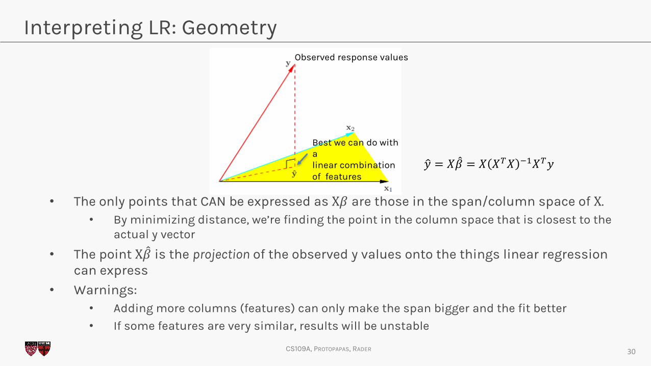
Interpreting LR: Geometry

• The only points that CAN be expressed as X𝛽 are those in the span/column space of X. • By minimizing distance, we’re finding the point in the column space that is closest to the

actual y vector

• The point X𝛽a is the projection of the observed y values onto the things linear regression can express

• Warnings: • Adding more columns (features) can only make the span bigger and the fit better

• If some features are very similar, results will be unstable

30

�̂� = 𝑋𝛽a = 𝑋 𝑋D𝑋 F8𝑋D𝑦

Observed response values

Best we can do with alinear combination of features

STATISTICSLinearRegression

31


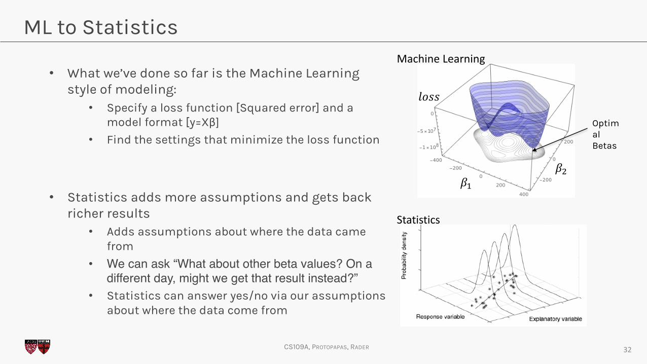
ML to Statistics

• What we’ve done so far is the Machine Learning style of modeling:

• Specify a loss function [Squared error] and a model format [y=Xβ]

• Find the settings that minimize the loss function

• Statistics adds more assumptions and gets back richer results

• Adds assumptions about where the data came from

• We can ask “What about other beta values? On a different day, might we get that result instead?”

• Statistics can answer yes/no via our assumptions about where the data come from

32

Statistics

𝛽8𝛽,

𝑙𝑜𝑠𝑠

MachineLearning

Optimal Betas


Statistical Assumptions

What are Statistics’ assumptions about the linear regression data?

• The observed X values simply are.

• The observed y come from a 𝑁𝑜𝑟𝑚𝑎𝑙(𝑚𝑢(𝑥), 𝑠𝑖𝑔𝑚𝑎)distribution, mu(x) is linear, and each y is drawn independently from the others• For all observations i: 𝑦g~𝑁 𝑥gβ, 𝜎,

• Equivalently, column y 𝑦~𝑁kl 𝑋𝛽, 𝜎,𝐼O

Why these assumptions?

• Any story about how the X data came to be is problem-dependent

• Makes the problem solvable using 1800s era tools

Question: How could we alter these assumptions? 33

Imagefrom:http://bolt.mph.ufl.edu/6050-6052/unit-4b/module-15/

𝜇g = 𝑥gβ 𝜎, unknownconstant

βvectorofunknownconstants

𝑦g~𝑁 𝜇g, 𝜎,


Maximum Likelihood: the other ML

• We need to guess at the unknown values (β and 𝜎,)

Maximum Likelihood

• Rule: Guess whatever values of the unknowns make the observed data as probable as possible• As a loss function, we feel pain when the data surprise the model

• Only works if we have a likelihood function• Likelihood maps (dataset) -> (probability of seeing that dataset); uses

parameter values (e.g. β and 𝜎,) in the calculation

• Actually maximizing can be hard

• But, Maximum Likelihood can be shown to be a very good guessing strategy, especially with lots of observations (see Stat 111 or 211)

34


Maximum Likelihood: the other ML

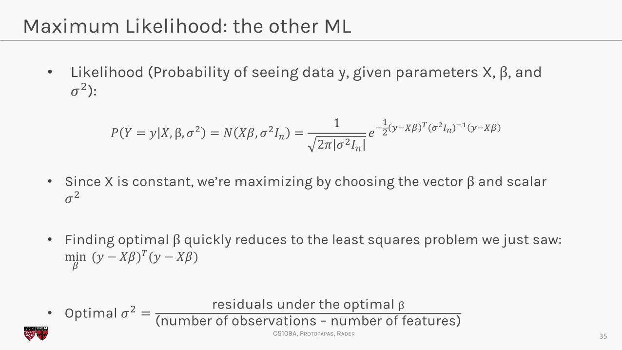
• Likelihood (Probability of seeing data y, given parameters X, β, and 𝜎,):

𝑃 𝑌 = 𝑦|𝑋, β, 𝜎, = 𝑁 𝑋𝛽, 𝜎,𝐼O =1

2𝜋 𝜎,𝐼O� 𝑒F

8, rFs` t(uvwx)yz rFs`

• Since X is constant, we’re maximizing by choosing the vector β and scalar 𝜎,

• Finding optimal β quickly reduces to the least squares problem we just saw: min`(𝑦 − 𝑋𝛽)D(𝑦 − 𝑋𝛽)

• Optimal 𝜎, = residuals under the optimal {(number of observations – number of features)

35


Benefits of assumptions

• We actually get the joint distribution of the betas: 𝛽|}~~𝑁(𝛽D��, 𝜎, 𝑋D𝑋 F8)

• HW investigates the variance term: how well we can learn each beta, and whether one is linked to another• It depends on X!

• It doesn’t depend on y! (If our assumptions are correct

• Lets us attach error bars to our estimates, e.g. 𝛽8 = 3 ± .2

• Main question: What can we do to our X matrix to

36


Review

• We can add assumptions about where the data came from and get richer statements from our model

• A Likelihood is a function that tells us how likely any given dataset is. Plug in data, get a probability

• The MLE finds the parameter settings that make our data as likely as possible

• Finding the MLE parameter values can be hard, sometimes possible via calculus, often requires computer code

37

STATISTICS: HYPOTHESIS TESTINGOR:WHATPARAMETERSEXPLAINTHEDATA

38


A Popper’s Grave

• It’s impossible to prove a model is correct• In fact, there are many correct

models

• Can you prove increasing a parameter by .0000001% is incorrect?

• We can only rule models out.

• The great tragedy is that you have been taught to rule out just ONE model, and then quit

39


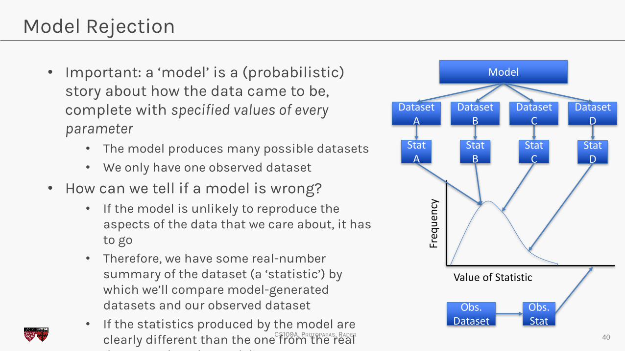
Model Rejection

• Important: a ‘model’ is a (probabilistic) story about how the data came to be, complete with specified values of every parameter

• The model produces many possible datasets

• We only have one observed dataset

• How can we tell if a model is wrong?• If the model is unlikely to reproduce the

aspects of the data that we care about, it has to go

• Therefore, we have some real-number summary of the dataset (a ‘statistic’) by which we’ll compare model-generated datasets and our observed dataset

• If the statistics produced by the model are clearly different than the one from the real data, we reject the model

40

Model

StatA

StatB

StatC

StatD

ValueofStatistic

Freq

uency

Obs.Dataset

Obs.Stat

DatasetA

DatasetB

DatasetC

DatasetD


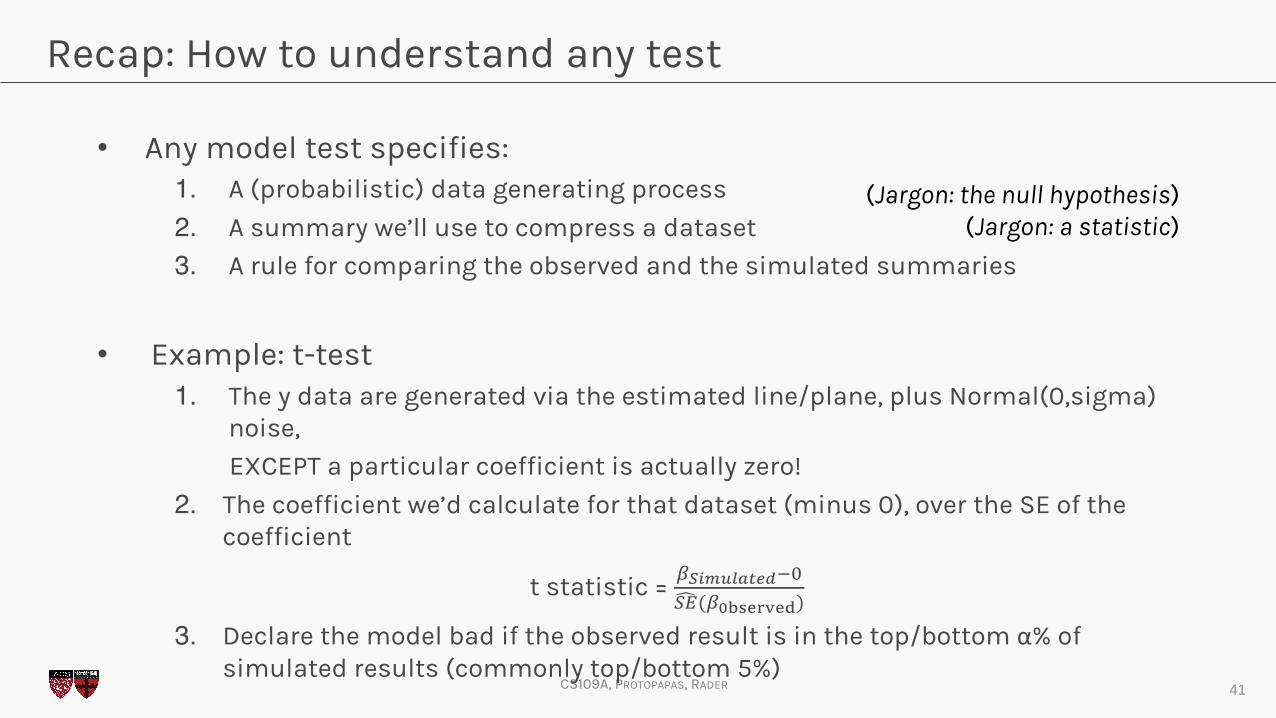
Recap: How to understand any test

• Any model test specifies:1. A (probabilistic) data generating process

2. A summary we’ll use to compress a dataset

3. A rule for comparing the observed and the simulated summaries

• Example: t-test1. The y data are generated via the estimated line/plane, plus Normal(0,sigma)

noise,

EXCEPT a particular coefficient is actually zero!

2. The coefficient we’d calculate for that dataset (minus 0), over the SE of the coefficient

t statistic = `��FB�~�(`��)

3. Declare the model bad if the observed result is in the top/bottom α% of simulated results (commonly top/bottom 5%)

41

(Jargon: the null hypothesis)(Jargon: a statistic)


The t-test

Walkthrough:

• We set a particular beta we care about to zero (call these betas 𝛽O��)

• We simulate 10,000 new datasets using 𝛽O�� as truth

• In each of the 10,000 datasets, fit a regression against X and plot the values of the 𝛽 we care about (the one we set to zero)

• The plotting the t statistic in each simulation is a little prettier

• The t statistic calculated from the observed data was 17.8. Do we think the proposed model generated our data?

42

• One more thing: Amazingly, ‘Student’ knew what results we’d get from the simulation

𝛽O�� = [2.2, 5, 0, 1.6]

𝛽�gk8 𝛽�gk, 𝛽�gk7 … 𝛽�gk8B,BBB

𝛽|}~ = [2.2, 5, 3, 1.6]T-testfor𝜷𝟐 =0

𝑋��𝜎|}~

𝑦�gk8 𝑦�gk, 𝑦�gk7 … 𝑦�gk8B,BBB

𝑋𝛽𝜎


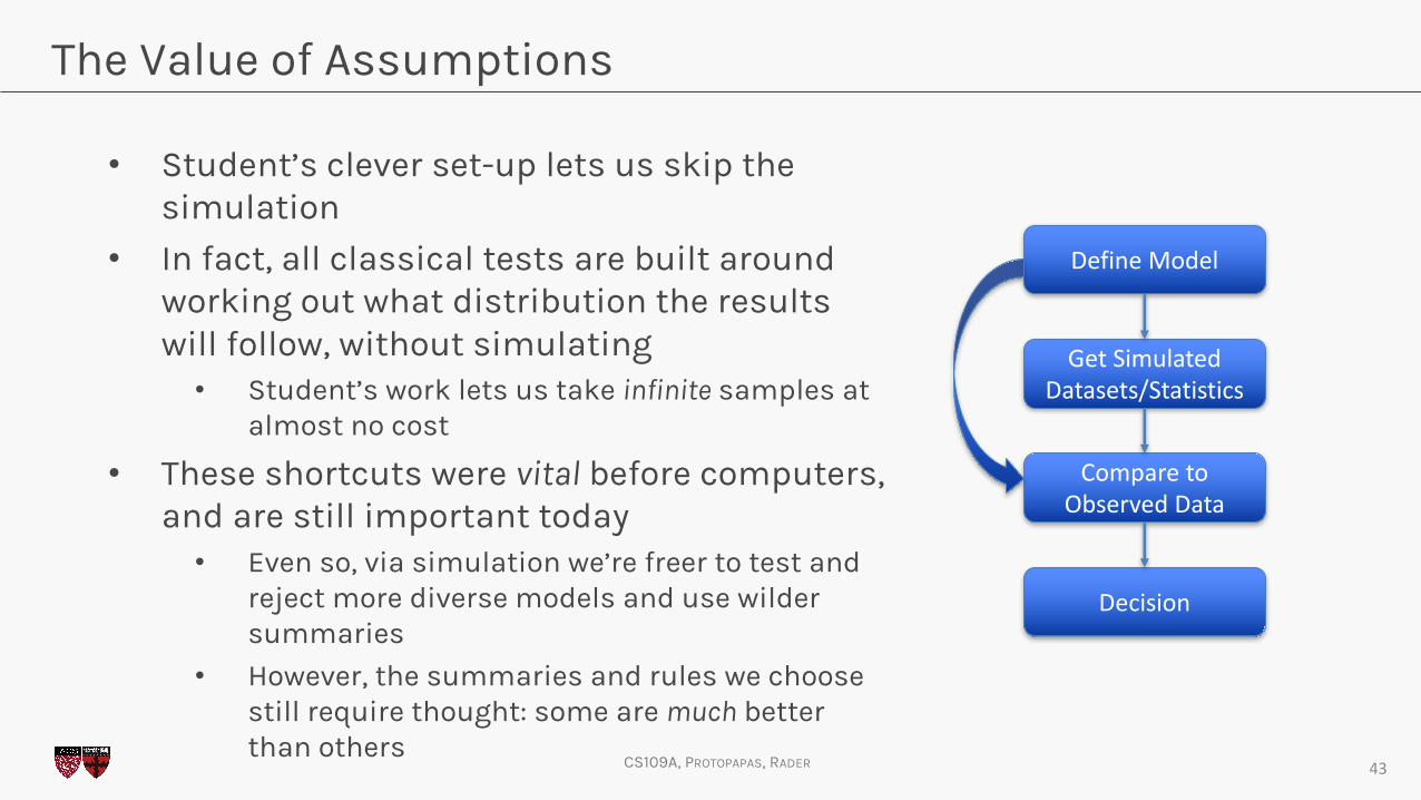
The Value of Assumptions

• Student’s clever set-up lets us skip the simulation

• In fact, all classical tests are built around working out what distribution the results will follow, without simulating• Student’s work lets us take infinite samples at

almost no cost

• These shortcuts were vital before computers, and are still important today• Even so, via simulation we’re freer to test and

reject more diverse models and use wilder summaries

• However, the summaries and rules we choose still require thought: some are much better than others

43

DefineModel

GetSimulatedDatasets/Statistics

ComparetoObservedData

Decision


p-values

• Hypothesis (model) testing leads to comparing a distribution against a point

• A natural way to summarize: report what percentage of results are more extreme than the observed data• Basically, could the model frequently

produce data that looks like ours?

• This is the p value: p=.031 means that your observed data is in the top 3.1% of weird results under this model+statistic• There is some ambiguity about what

‘weird’ should mean

Jargon: p values are “The probability, assuming the null model is exactly true, of seeing a value of [your statistic] as extreme or more extreme than what was seen in the observed data” 44

ResultsFromSimulation

Freq

uency Resultsfromobserved

dataset

DistributionofSimulationResults

Simulationsweirderthantheobserveddata

?


p Value Warnings

• p values are only one possible measure of the evidence against a model

• Rejecting a model when p<threshold is only one possible decision rule• Get a book on Decision Theory for more

• Even if the null model is exactly true, 5% of the time, we’ll get a dataset with p<.05• p<.05 doesn’t prove the null model is wrong

• It does mean that anyone who wants to believe in the null must explain with why something unlikely happened

45


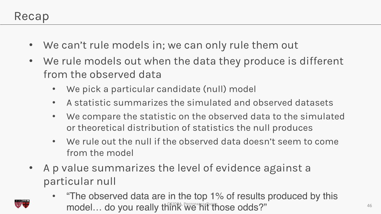
Recap

• We can’t rule models in; we can only rule them out

• We rule models out when the data they produce is different from the observed data• We pick a particular candidate (null) model

• A statistic summarizes the simulated and observed datasets

• We compare the statistic on the observed data to the simulated or theoretical distribution of statistics the null produces

• We rule out the null if the observed data doesn’t seem to come from the model

• A p value summarizes the level of evidence against a particular null• “The observed data are in the top 1% of results produced by this

model… do you really think we hit those odds?” 46

STATISTICS: HYPOTHESIS TESTINGCONFIDENCEINTERVALSANDCOMPOSITEHYPOTHESES

47


Recap

• Let’s talk about what we just did• That t-test was ONLY testing the model where the coefficient in question is

set to zero

• Ruling out this model makes it more likely that other models are true, but doesn’t tell us which ones

• If the null is β = 0, getting p<.05 only rules out THAT ONE model

• When would it make sense to stop after ruling out β = 0, without testing β = .1?

48

DawnofTime

β =-.3 β =-.2 β =-.1 β =0 β =.1 β =.2 β =.3

OurData

β =-.4 β =-.4


Composite Hypotheses: Multiple Models

• Often, we’re interested in trying out more than one candidate model

• E.g. Can we disprove all models with a negative value of beta?

• This amounts to simulating data from each of those models (but there are infinitely many…)

• Sometimes, ruling out the nearest model is enough; we know that the other models have to be worse

• If a method claims it can test θ<0, this is how

49

ββ=MLEβ=0

Canweruletheseout?

β=0willbeclosertomatchingthedata(intermsoftstatistic)thananyothermodelintheset*;weonlyneedtotestβ=0*Non-trivial;trueforstudent’stbutnotforothermeasures


β =-.2β =-.4

THE Null vs A Null

• What if we tested LOTS of possible values of beta?• Special conditions must hold to avoid multiple-testing issues; again, the t test model+statistic

pass them

• We end up with a set/interval of surviving values, e.g. [.1,.3]• Sometimes, we can directly calculate what the endpoints would be

• Since each beta was tested under the rule “reject this beta if the observed results are in the top 5% of weird datasets under this model”, we have [.1,.3] as a 95% confidence interval

50

DawnofTime

OurData

β =0 β =.1 β =.2 β =.3β =-.1β =-.3 β =-.4


Confidence Interval Warnings

• WARNING: This kind of accept/reject confidence interval is rare• Most confidence intervals do not map accept/reject regions of a (useful)

hypothesis test

• A confidence interval that excludes zero does not usually mean a result is statistically significant• Statistically significant: The data resulting from an experiment/data collection have p<.05 (or

some other threshold) against a no-effect model, meaning we reject the no-effect model

• It depends on how that confidence interval was built

• A confidence interval’s only promise: if you were to repeatedly re-collect the data and build 95% CIs, (assuming our story about data generation is correct) 95% of the intervals would contain the true value

51


Confidence Interval Warnings

• WARNING: A 95% confidence interval DOES NOT have a 95% chance of holding the true value• There may be no such thing as “the true value”, b/c the model is

wrong

• Even if the model is true, a “95% chance” statement requires prior assumptions about how nature sets the true value

• Stick around after section for a heartbreaking demo of why a group of confidence intervals make 95% but any particular CI can be 0%, 100%, or anything in between

52


HW Preview

• The 209 homework touches on another kind of confidence interval• Class: “How well have I estimated beta?”• HW: “How well can I estimate the mean response at each X?”• Bonus: “How well can I estimate the possible responses at each

X”?

53


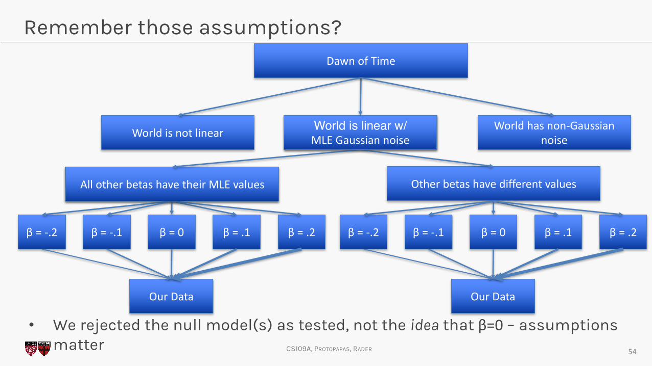
Remember those assumptions?

54

DawnofTime

β =-.2 β =-.1 β =0 β =.1 β =.2

OurData

DawnofTime

AllotherbetashavetheirMLEvalues Otherbetashavedifferentvalues

DawnofTime

Worldisnotlinear Worldhasnon-Gaussiannoise

World is linear w/ MLEGaussiannoise

β =-.2 β =-.1 β =0 β =.1 β =.2

OurData

• We rejected the null model(s) as tested, not the idea that β=0 – assumptions matter


Review

• Ruling out a single model isn’t much

• Sometimes, ruling out a single model is enough to rule out a whole class of models

• Assumptions our model makes are weak points that should be justified and checked for accuracy

• Confidence intervals give a reasonable idea of what some unknown value might be

• Any single confidence intervals cannot give a probability

• Statistical significance is 99% unrelated to confidence intervals

55

STATISTICS: REVIEWYoumadeit!

56


Review

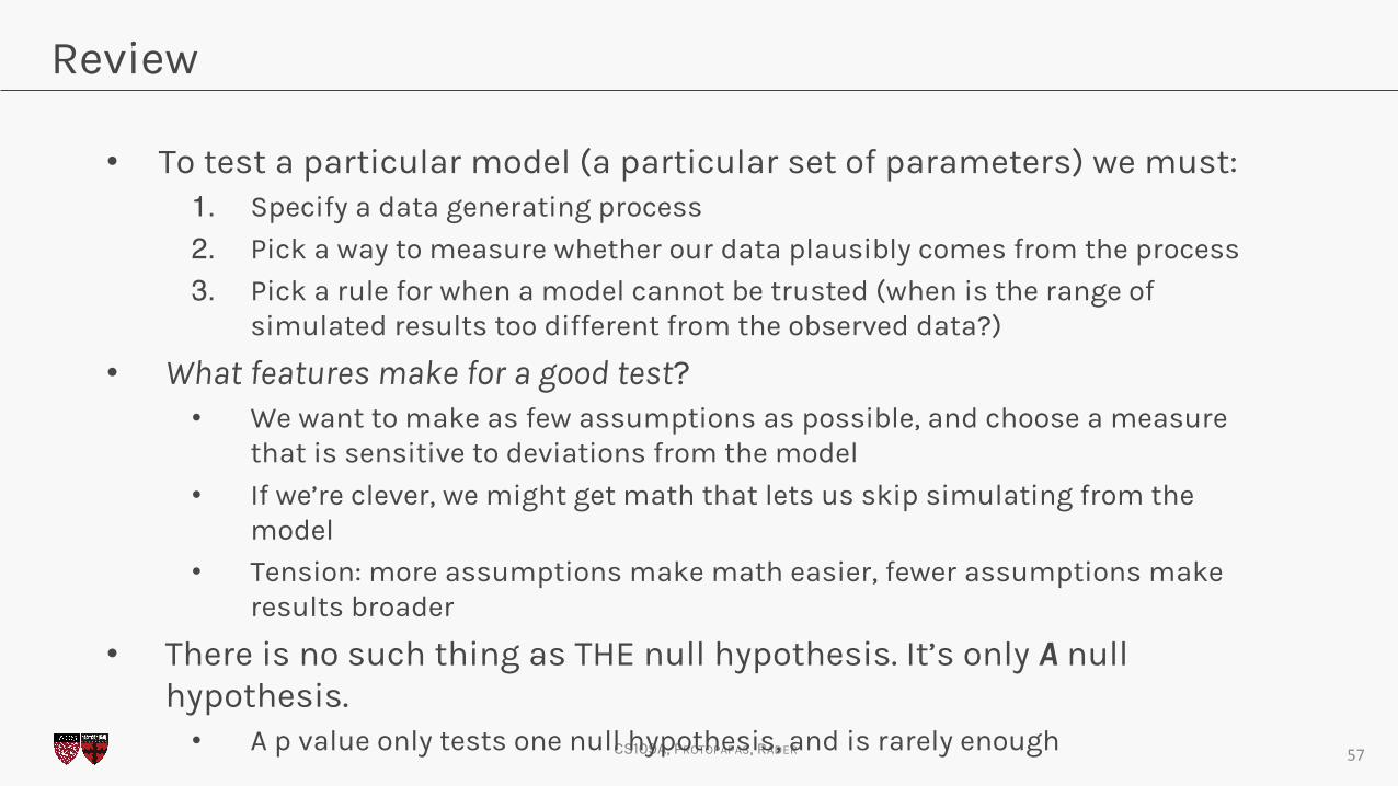
• To test a particular model (a particular set of parameters) we must:1. Specify a data generating process

2. Pick a way to measure whether our data plausibly comes from the process

3. Pick a rule for when a model cannot be trusted (when is the range of simulated results too different from the observed data?)

• What features make for a good test?• We want to make as few assumptions as possible, and choose a measure

that is sensitive to deviations from the model

• If we’re clever, we might get math that lets us skip simulating from the model

• Tension: more assumptions make math easier, fewer assumptions make results broader

• There is no such thing as THE null hypothesis. It’s only A null hypothesis.• A p value only tests one null hypothesis, and is rarely enough 57


Going forward

As the course moves on, we’ll see

• Flexible assumptions about the data generating process• Generalized Linear Models

• Ways of making fewer assumptions about the data generating process:• Bootstrapping

• Permutation tests

• Easier questions: Instead of ‘find a model that explains the world’, ‘pick the model that predicts best’• Validation sets and cross validation

58


Thank you

Office hours are:

Monday 6-7:30 (Camilo)

Tuesday 6:30-8 (Will)

59


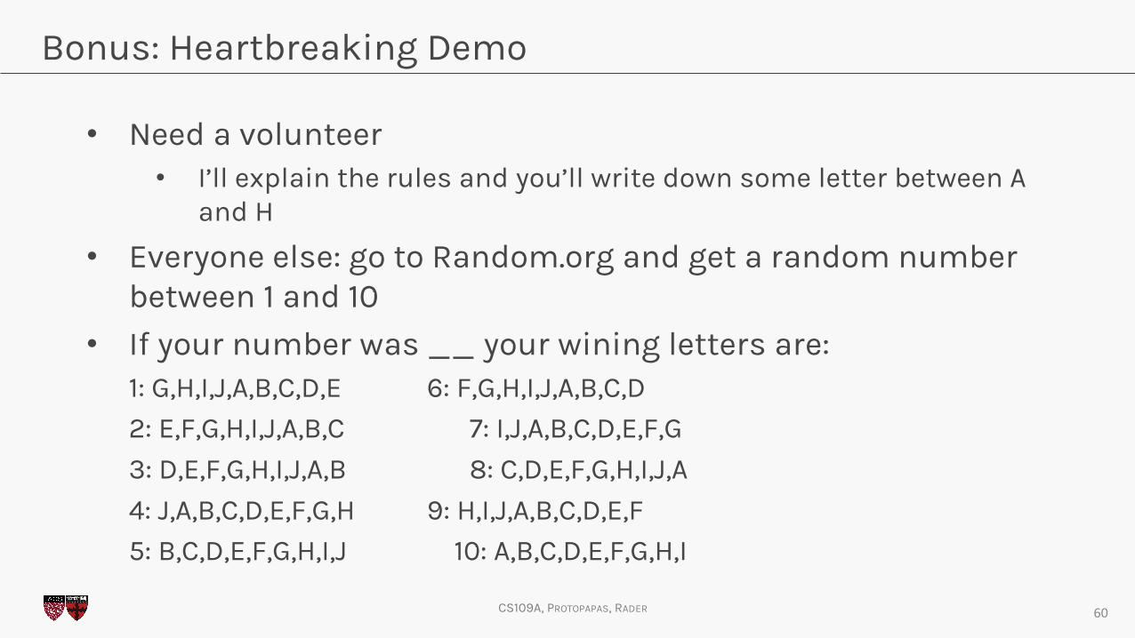
Bonus: Heartbreaking Demo

• Need a volunteer• I’ll explain the rules and you’ll write down some letter between A

and H

• Everyone else: go to Random.org and get a random number between 1 and 10

• If your number was __ your wining letters are: 1: G,H,I,J,A,B,C,D,E 6: F,G,H,I,J,A,B,C,D

2: E,F,G,H,I,J,A,B,C 7: I,J,A,B,C,D,E,F,G

3: D,E,F,G,H,I,J,A,B 8: C,D,E,F,G,H,I,J,A

4: J,A,B,C,D,E,F,G,H 9: H,I,J,A,B,C,D,E,F

5: B,C,D,E,F,G,H,I,J 10: A,B,C,D,E,F,G,H,I

60

advanced section #1: linear algebra and hypothesis testing · advanced section 1 today’s topics:...

Documents