Advanced Microarray Analysis Course

Day 4: Integrative Analysis

PJ “Asa” Wirapati

BioinformaticsCore Facility

Swiss Instituteof Bioinformatics

Lausanne, 3 November 2009

1

Today’s Topics

• Genome-wide scans and summary statistics

• Comparing genome-wide summary profiles

• Combined analysis

2

Overview

We’ve seen different types of regression analysis and unsupervisedmethod such as normal mixture models.

They can be applied to:

• Each gene separately (typically correlating to a certain variable,e.g. phenotype)

• Pairs of genes (such as in hierarchical clustering, or trying tofind pairs than predict a response)

• Multiple variables in the problem of building classifiers.

• Dependency network reconstruction (where a respone variablein one model is a predictor in some other models)

We’ll focus on the first one.

3

Genome/Transcriptome Scan

Basic idea:

• Formulate a question in terms of the appropriate statistical model(specific regression formula, mixture model, etc.), involving oneunknown variable (usually a gene) and some fixed ones. Theunknown can be response or explanatory variable in a regression(whichever is appropriate).

• Fit the model to each gene, separately (“scan” the genome)

• Choose some summary statistics to select/rank interesting genes(e.g. test of significance, fold-change, etc.)

• Often a cutoff (e.g. corrected p-value, FDR) is chosen to binarizethe summaries, to produce “significant” gene list. This may not beoptimal in the context of integrative analysis.

4

Types of summary statistics

Effect size : regression coefficients, model parameters

Measure strength of physical/biological relationship

⇒ The scale (unit of measurement) has to be meaningful

Dependency : Pearson’s correlation, R2, mutual information, etc.

How much we can predict; “proportion of explained variation”

⇒ The scale doesn’t matter, but the design (sampling criteria) does

Significance : p-value, t-stat, Z-test, deviance, etc.

Strength of evidence

⇒ reflects the strength of the study design (sample size, methodology,

etc.) and strength of relationship, but the role of each isn’t clear

Decision : accept or reject, gene lists, “signatures”

Which hypothesis (null or alternative) generates the observations

⇒ depends on the choice of cut-off (acceptable trade-off between “risk”

and “reward”)

5

An example

1. We are interested in metastasis-free survival in breast cancer

2. Use simple formulation:coxph(Surv(t.mfs,d.mfs) ∼ gex[,i]) ,

applied to every single gene i

3. Extract relevant summary statistics:

• Trivial stats: mean, SD of expression values

• Effect size: the estimate of coefficient and its SE

• Dependence/correlation: standardized coeff. and its SE[In this case (with no other covariates): coeff times SD]

• Log likelihood (alternate measure of significance)

• Sample size and number of events per gene (not necessarilythe same for all genes due to missing values)

Significance, p-value, rank, FDR, etc. are derived from the above.

6

Demo of an example summary table

Load data and scripts

Examine table headers

Plot (histogram, scatter, etc.) some (pairs of) summaries

Learn nplot (or others) and identify function

Derive Z-scores, p-value, deviance

Derive pseudo R2

(Near) equivalence of some of the summaries

Comparing significance, effect size, correlation (volcano plots)

7

Selecting interesting genes

Ranking is typically based on significance, not effect size (because ofgene-specific standard error), nor correlation/R2 (because it’s nearlyidentical to significance since each variable has the same sample size).

Effect size criteria are used informally, in conjuction with significance(Volcano plot).

Cutoff is decided by various criteria.

• The traditional one: p-value with multiple testing correction (e.g.Bonferroni)

• False discovery rate (e.g. Benjamini-Hochberg): treat the summarydistribution as a kind of mixture, with most genes generated by thenull, and interesting ones are outliers

[Demo: histogram Z-score, p-value, scatter plots; use p.adjust()]

8

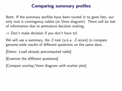
Comparing summary profiles

Note: If the summary profiles have been turned in to gene lists, ouronly tool is contingency tables (or Venn diagram). There will be lostof information due to premature decision making.

⇒ Don’t make decision if you don’t have to!

We will use a summary, the Z-test (a.k.a. Z-score) to comparegenome-wide results of different questions on the same data.

[Demo: Load already precomputed table]

[Examine the different questions]

[Compare overlap/Venn diagram with scatter plot]

9

SwissBrodSwiss Breast Oncogenomic Database

SusanneKunkel

Dataset No. of Institution Reference Platform Data source No. ofsymbol arrays GeneIDs

Genomic platformsNKI 337 Nederlands Kanker Instituut van’t Veer 2002, van de Vijver 2002 Agilent author’s website 13120EMC 286 Erasmus Medical Center Wang 2005 Aff. U133A GEO:GSE2034 11837UPP 249 Karolinksa Institute (Uppsala) Miller 2005, Calza 2006 Aff. U133A,B GEO:GSE4922 15684STOCK 159 Karolinska Institute (Stockholm) Pawitan 2005, Calza 2006 Aff. U133A,B GEO:GSE1456 15684DUKE 171 Duke University Huang 2005, Bild 2006 Aff. U95Av2 author’s website 8149UCSF 161+8 UC San Francisco Korkola 2003 cDNA author’s website 6178UNC 143+10 University of Carolina Hu 2006 Agilent HuA1 author’s website 13784NCH 135 Nottingham City Hospital Naderi 2006 Agilent HuA1 AE:E-UCON-1 13784STNO 115+7 Stanford Univ./Norwegian Radium Hosp. Sorlie 2003 cDNA author’s website 5614JRH1 99 John Radcliffe Hospital Sotiriou 2003 cDNA journal’s website 4112JRH2 61 John Radcliffe Hospital Sotiriou 2006 Aff. U133A GEO:GSE2990 11837MGH 60 Massachusetts General Hospital Ma 2004 Agilent GEO:GSE1379 11421

expO 239 International Genomic Consortium http://www.intgen.org Aff. U133v2 GEO:GSE2109 16634TGIF1 49 EORTC trial 10994 Farmer 2005 Aff. U133A GEO:GSE1561 11837BWH 40+7 Brigham and Women’s Hospital Richardson 2006 Aff. U133v2 GEO:GSE3744 16634

Small diagnostic platformsTRANSBIG 253 TRANSBIG Consortium Buyse 2006 Agilent AE:E-TABM-77 1052EMC2 180 Erasmus Medical Center Foekens 2006 Aff. (custom) GSE3453 86HPAZ 96 Hospital La Paz, Madrid Espinosa 2005 RT-PCR paper’s appendix 61

Total 2865 = 2833 carcinomas No. of the union of all GeneIDs: 17198+ 32 non-malignant breast tissues No. of GeneIDs common to genomic platforms: 1963

• Abbreviations: No. = number, GEO: = Gene Expression Omnibus accession, AE: = ArrayExpress accession, Aff. = Affymetrix

• Curation: (re)group datasets into independent, non-redundant cohorts• Few genes are common to all platforms ⇒ use the union, not the intersection

10

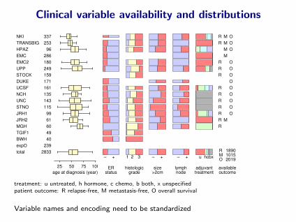
Clinical variable availability and distributions

NKI 337TRANSBIG 253HPAZ 96EMC 286EMC2 180UPP 249STOCK 159DUKE 171UCSF 161NCH 135UNC 143STNO 115JRH1 99JRH2 61MGH 60TGIF1 49BWH 40expO 239total 2833

25 50 75 100age at diagnosis (year)

– +

ERstatus

1 2 3

histologicgrade

– +

size>2cm

– +

lymphnode

u hcbx

adjuvanttreatment

R M OR M O

M OM

R OR OR O

OR OR OR OR OR OR MR

R 1890M 1015O 2019

availableoutcome

treatment: u untreated, h hormone, c chemo, b both, x unspecifiedpatient outcome: R relapse-free, M metastasis-free, O overall survival

Variable names and encoding need to be standardized

11

Heterogeneity in survival data

total 6311890 1415 1147 799 469

STNO 60115 39 10 1UNC 32128 33 10 4JRH1 4599 75 59 30 1MGH 2560 50 42 28 18NCH 47135 110 97 81 66NKI 121319 260 216 131 75TRANSBIG 101253 207 170 147 118UPP 88249 185 158 140 107JRH2 1561 55 44 38 33STOCK 40159 140 124 68EMC2 37180 164 149 94 40UCSF 20132 97 68 37 11

STNOUNCJRH1MGH

NCH

NKITRANSBIGUPP

JRH2STOCK

EMC2UCSF

40

60

80

100

rela

pse-

free

surv

ival (

%)

group: number at risk: eventsfollow-up: 0 2.5 5 7.5 10 (year)

total 4842019 1628 1313 867 512

STNO 46115 54 14 3 1DUKE 43170 86 46 12 3UNC 22129 39 14 5JRH1 4599 85 70 32 1UCSF 37132 104 74 43 14NKI 74319 290 248 147 89STOCK 40159 148 130 64NCH 34135 122 111 96 81TRANSBIG 57253 240 212 190 154UPP 51232 198 173 152 122EMC2 23180 175 166 103 44HPAZ 1296 87 55 20 3

STNODUKE

UNC

JRH1

UCSFNKI

STOCKNCH

TRANSBIGUPPEMC2HPAZ

40

60

80

100

over

all s

urviv

al (%

)

group: number at risk: eventsfollow-up: 0 2.5 5 7.5 10 (year)

Variability between studies greater than that due to natural risk factors ortreatments ⇒ typical in retrospective studies

12

Quirks in the original normalized data

Plot SD-vs-mean of each probe in a dataset⇒ A characteristic trend for each (platform,normalization) combo

NKI: Agilent (Rosetta) + ? EMC: Affy U133 + MAS 5.0 TGIF1: Affy U133A + RMA

Raw data for renormalization from scratch not always available⇒ post-hoc correction:

13

Emerging Statistical/Computational Challenges

Adapt to multi-dataset contexts:

• Gene-by-gene association or differential expression

• Clustering of genes (to find coexpression modules)

• Clustering of patients (to find disease subtypes)

• Prediction/classification

• Others, e.g. mixture models

The first one has been addressed, to some extent, by borrowingtechniques from meta analysis

14

A spectrum of approaches to combined estimates

1. Pool (treat as a single cohort)

assume the data can be “normalized” somehow beforehand

2. Fixed-effect models

study-specific nuisance parameters (e.g. as covariates)

3. Hierarchical/multilevel/mixed/empirical Bayes models

stages of sampling, with between study variance; shrinkage

4. Combined significance measures

e.g., Z-test (inverse normal), p-value (Fisher’s or inverse χ2)

5. Combined ranks or decisions

e.g., Venn diagram, overlaps, vote counting

The extremes are more easily applicable and, hence, popular

15

Illustration: Berkeley grad school admission 1973

A

B

C

D

E

F

0.25 0.5 1 2

­ women ­ menodds ratio

Pooled

FE

REΣ0

2

Q = 19.9, p = 0.003

combined Z-test = -1.46, p = 0.14vote count: 1�6 significant ­women

Problem with pooling:“The whole can be outside the range of its parts”

• Simpson’s (reversal) paradox

(e.g. this example)

• attenuation of effect size

(e.g. when pooling centered variables)

FE: total under fixed-effect model

β =P

i βi/σ2i

. Pi 1/σ2

i

RE: total under random-effect model

β0 =P

i βi/(σ20 + σ2

i ). P

i 1/(σ20 + σ2

i )

σ20 : random effect variance (between strata)

Q: Cochran’s heterogeneityP

i(yi− µ)2/σ2i ∼ χ

2k−1

Combined Z-test:P

i Zi/√k

16

Hierarchical Modelsβ0

ww��

((βi ∼ N(β0, σ

20) β1

��

· · · βi

��

· · · βk

��

β

Yij ∼ f(βi, σ2i ) Y 1 · · · Y i · · · Y k

?>=<89:;?

BC

EDREoo

//

FE

OO

Single study:

• Inference about βi (β0 + study bias: technical, design,. . . )

Fixed-effect models

• Inference about β =P

i βi/k (mean of the specific set in hand)

• C.I. not affected by between study variability σ20

Random-effect/hierarchical models

• Inference about β0 (the “truth”; expectation of future studies)

• When Q is small behaves like FE models (weighted average);when Q is large, behaves like the “average-of-average” (insensitive toimbalance in study precisions)

17

Genome-wide scan of summary statistics

Venn diagram

160 27 411

overlap fixed-effect random-effect

18

Which quantity should be linked across studies?

Example: breast cancer survival vs expression (Cox proportional hazard).For an example gene:

MELK

-1 0 1 2beta, coefficient

DUKE 43/170EMC 107/286EMC2 0/0HPAZ 25/96JRH1 45/98JRH2 15/61MGH 0/0NKI 109/319STNO 0/0STOCK 40/159UCSF 0/0UNC 22/128UPP 53/232NCH 35/135TRANSBIG 67/253

FE mean, CI p=1e-12heterogeneity Q=42.3RE sigma0^2RE mean, CI p=6e-05

0 0.5 1Z/sqrt(Ne), correlation

p=4e-19 Q=7.6

p=4e-19

0 2.5 5 7.5 10Z-test, significance

p=2e-18 Q=11.2

p=2e-16

-log10(p)0 1 2 3 4

p = 1e-14 chi^2 = 115.1 df = 2 x 11

-log10(rank/m)0 1 2

p = 8e-08 chi^2 = 75.8 df = 2 x 11

FWER

––

–––

–

–

––––

FDR

––

–––

+

–

–+––

19

AURKA

-0.5 0 0.5 1 1.5beta, coefficient

DUKE 43/170EMC 107/286EMC2 0/0HPAZ 0/0JRH1 44/98JRH2 15/61MGH 28/60NKI 109/319STNO 46/115STOCK 40/159UCSF 38/132UNC 22/129UPP 53/232NCH 35/135TRANSBIG 67/253

FE mean, CI p=4e-19heterogeneity Q=21.1RE sigma0^2RE mean, CI p=6e-13

0 0.5 1 1.5Z/sqrt(Ne), correlation

p=3e-20 Q=13.3

p=6e-18

0 5 10Z-test, significance

p=1e-17 Q=24.9

p=3e-09

-log10(p)0 2.5 5

p = 2e-15 chi^2 = 128.0 df = 2 x 13

-log10(rank/m)0 1 2 3

p = 2e-07 chi^2 = 80.5 df = 2 x 13

FWER

––

–––+–––––––

FDR

–+

–––+–––––––

20

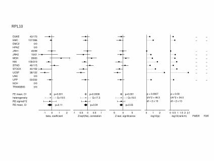
RPL10

-1 0 1 2beta, coefficient

DUKE 43/170EMC 107/286EMC2 0/0HPAZ 0/0JRH1 45/99JRH2 15/61MGH 28/60NKI 109/319STNO 46/115STOCK 40/159UCSF 38/132UNC 0/0UPP 53/232NCH 0/0TRANSBIG 0/0

FE mean, CI p=0.001heterogeneity Q=19.5RE sigma0^2RE mean, CI p=0.11

-1 -0.5 0 0.5 1Z/sqrt(Ne), correlation

p=0.0006 Q=17.3

p=0.04

-5 0 5Z-test, significance

p=0.001 Q=19.0

p=0.03

-log10(p)0 1 2

p = 0.0007 chi^2 = 46.3 df = 2 x 10

-log10(rank/m)0 0.5 1 1.5 2 2.5

p = 0.03 chi^2 = 34.0 df = 2 x 10

FWER

––

–––––––

–

FDR

––

–––––––

–

21

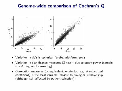
Genome-wide comparison of Cochran’s Q

• Variation in βi’s is technical (probe, platform, etc.)

• Variation in significance measures (Z-test): due to study power (samplesize & degree of censoring)

• Correlation measures (or equivalent, or similar, e.g. standardizedcoefficient) is the least variable: closest to biological relationship(although still affected by patient selection)

22

Genome-Wide Applications

23

Hierarchical Agglomerative Clustering of Genes

(Clustering arrays is a different problem)

• Use hierarchical model for pairwise Pearson correlations rijk(i studies, j, k genes)

• Transform to approximately normal quantities:

zijk = tanh−1(rijk), Var(zijk) = 1/(n− 3)ortijk = rijk√

1−r2ijk

, Var(tijk) = 1/(n− 2)

• Treat the combined correlations as similarity measures inhierarchical agglomerative clustering. No need to backtransform.

• Display the heatmaps in stratified manner

24

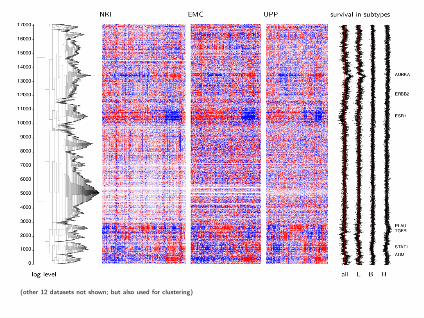
(other 12 datasets not shown; but also used for clustering)

25

26

Glioblastoma (courtesy of Eugenia Miggliavacca)

27

Colon cancer (courtesy of Mauro Delorenzi)

28

Between array correlationsUse pairwise correlations (using variable genes)Each pair of studies (platforms) has its own common genesPool all correlation, make a single tree, use the ordering

glioblastoma colon

So far, performed separately per disease (cancer type)

Additional sampling hierarchy: disease → studies → patients

29

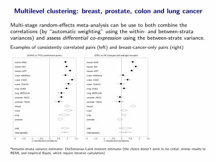
Multilevel clustering: breast, prostate, colon and lung cancer

Multi-stage random-effects meta-analysis can be use to both combine thecorrelations (by “automatic weighting” using the within- and between-stratavariances) and assess differential co-expression using the between-strate variance.

Examples of consistently correlated pairs (left) and breast-cancer-only pairs (right)

-2 -1.5 -1 -0.5 0 0.5 1 1.5z-transformed correlations

AURKA vs TPX2 Hproliferation genesL

breast-EMC

breast-NKI

breast-UPP

colon-AARHUS

colon-CINCI

colon-TOKYO

lung-DUKE

lung-MERLION

prostate-SKCC

prostate-TMHS

breast

colon

lung

prostate

total

heterogeneity

-2 -1.5 -1 -0.5 0 0.5 1 1.5z-transformed correlations

ESR1 vs AR Hestrogen and androgen receptorL

breast-EMC

breast-NKI

breast-UPP

colon-AARHUS

colon-CINCI

colon-TOKYO

lung-DUKE

lung-MERLION

prostate-SKCC

prostate-TMHS

breast

colon

lung

prostate

total

heterogeneity

*between-strata variance estimator: DerSimonian-Laird moment estimator (the choice doesn’t seem to be critial; similar results toREML and empirical Bayes, which require iterative calculation)

30

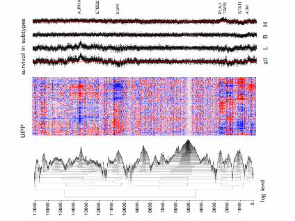
breast cancer

Dendogram of 16742 genes NKI EMC UPP

1000

2000

3000

4000

5000

6000

7000

8000

9000

10000

11000

12000

13000

14000

15000

16000

proliferation

estrogen receptor

androgen receptor

stroma

ERBB2

EGFR

immuneresponse

"junk"

branch depth: log(level) n = 337 n = 286 n = 249

31

prostate cancer colon cancer lung cancer

SKCC TMHS AARHUS CINCI TOKYO DUKE MERLION

n = 148 n = 65 n = 155 n = 105 n = 84 n = 198 n = 72

32

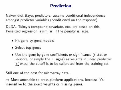
Prediction

Naıve/idiot Bayes predictors: assume conditional independenceamongst predictor variables (conditioned on the response).

DLDA, Tukey’s compound covariate, etc. are based on this.Penalized regression is similar, if the penalty is large.

• Fit gene-by-gene models

• Select top genes

• Use the gene-by-gene coefficients or significance (t-stat orZ-score, or simply the ± signs) as weights in linear predictor:∑wixi; the cutoff is to be calibrated from the training set

Still one of the best for microarray data.

⇒ Most amenable to cross-platform applications, because it’sinsensitive to the exact weights or missing genes.

33

Cross validation schemes

1. Within dataset

• Split each dataset into learning and test parts

• Select top genes (ranking based on total significance)

• In each dataset, apply the model with dataset-specificparameters to the test part

• Combine performance

2. Cross-dataset

• Split datasets into learning and test datasets

• Fit model in the test datasets

• Apply to test datasets: global weights, local cutoff (needits own CV)

⇒ “Leave-one-dataset out CV” is particularly simple

34

Example of LODOCV: Breast cancer datasets

Use Z-test as weights in linear predictor

Cutoff is 30% low-risk

total 6752426 1913 1533 1029 592

hi-risk 5561633 1216 941 617 363lo-risk 119793 697 592 412 229

hi-risk

lo-risk

0

20

40

60

80

100

DMFS

(%)

group: number at risk: eventsfollow-up: 0 2.5 5 7.5 10 (year)

DUKEEMCEMC2HPAZJRH1JRH2MGHNKISTNOSTOCKUCSFUNCUPPNCHTRANSBIGTotal

0 25 50 75 1005-year DMFS (%)

hi-risk lo-risk

hazard ratio1 3 10 30

35

Summary

Hierarchical models can be used to co-analyze datasets from multiplestudies

Random-effect meta-analysis is a decent approximation to analyzingall raw data in a stratified/hierarchical manner.

Heterogeneity/consistency is an important property that should beintegral part of the analysis and presentation

More works are needed to embed hierarchical models into othermodes of analysis: finite mixture models, conditional independentgraphs (dependency networks), . . .

36