advanced integration techniques.pdf
DESCRIPTION
mathTRANSCRIPT

Chapter 7
Advanced Integration Techniques
Before introducing the more advanced techniques, we will look at a shortcut for the easier of thesubstitution-type integrals. Advanced integration techniques then follow: integration by parts,trigonometric integrals, trigonometric substitution, and partial fraction decompositions.
7.1 Substitution-Type Integration by Inspection
In this section we will consider integrals which we would have done earlier by substitution, butwhich are simple enough that we can guess the approximate form of the antiderivatives, andthen insert any factors needed to correct for discrepancies detected by (mentally) computing thederivative of the approximate form and comparing it to the original integrand. Some generalforms will be mentioned as formulas, but the idea is to be able to compute many such integralswithout resorting to writing the usual u-substitution steps.
Example 7.1.1 Compute
∫
cos 5xdx.
Solution: We can anticipate that the approximate form1 of the answer is sin 5x, but then
d
dxsin 5x = cos 5x · d
dx(5x) = cos 5x · 5 = 5 cos 5x.
Since we are looking for a function whose derivative is cos 5x, and we found one whose derivativeis 5 cos 5x, we see that our candidate antiderivative sin 5x gives a derivative with an extra factorof 5, compared with the desired outcome. Our candidate antiderivative’s derivative is 5 timestoo large, so this candidate antiderivative, sin 5x must be 5 times too large. To compensate andarrive at a function with the proper derivative, we multiply our candidate sin 5x by 1
5 . This giveus a new candidate antiderivative 1
5 sin 5x, whose derivative is of course 15 cos 5x · 5 = cos 5x, as
desired. Thus we have ∫
cos 5xdx =1
5sin 5x + C.
It may seem that we wrote more in the example above than with the usual u-substitutionmethod, but what we wrote could be performed mentally without resorting to writing the details.
In future sections, an integral such as the above may occur as a relatively small step in theexecution of a more advanced and more complicated method (perhaps for computing a muchmore difficult integral). This section’s purpose is to point out how such an integral can be quicklydispatched, to avoid it becoming a needless distraction in the more advanced methods.
1In this section, by approximate form we mean a form which is correct except for multiplicative constants.
591

592 CHAPTER 7. ADVANCED INTEGRATION TECHNIQUES
7.1.1 The Method
The method used in all the examples here can be summarized as follows:
1. Anticipate the form of the antiderivative by an approximate form (correct up to a multi-plicative constant).
2. Differentiate this approximate form and compare to the original integrand function;
3. If Step 1 is correct, i.e., the approximate form’s derivative differs from the original integrandfunction by a multiplicative constant, insert a compensating, reciprocal multiplicative con-stant into the approximate form to arrive at the actual antiderivative;
4. For verification, differentiate the answer to see if the original integrand function emerges.
For instance, some general formulas which should be quickly verifiable by inspection (thatis, by reading and mental computation rather than with paper and pencil, for instance) follow:
∫
ekx dx =1
kekx + C, (7.1)
∫
cos kx dx =1
ksinkx + C, (7.2)
∫
sin kx dx = −1
kcos kx + C, (7.3)
∫
sec2 kx dx =1
ktankx + C, (7.4)
∫
csc2 kx dx = −1
kcotkx + C, (7.5)
∫
sec kx tan kx dx =1
ksec kx + C, (7.6)
∫
csc kx cot kx dx = −1
kcsc kx + C, (7.7)
∫1
ax + bdx =
1
aln |ax + b|+ C. (7.8)
Example 7.1.2 The following integrals can be computed with u-substitution, but also are com-putable by inspection:� ∫
e7x dx =1
7e7x + C,� ∫
1
5x− 9dx =
1
5ln |5x− 9|+ C,� ∫
sin 5xdx = −1
5cos 5x + C,
� ∫
cosx
2dx = 2 sin
x
2+ C,� ∫
sec2 πxdx =1
πtanπx + C,� ∫
csc 6x cot 6xdx = −1
6csc 6x + C.
While it is true that we can call upon the formulas (7.1)–(7.8), the more flexible strategy isto anticipate the form of the antiderivative and adjust accordingly. For instance, we have thefollowing antiderivative form, written two ways:
∫1
udu = ln |u|+ C,
∫f ′(x)
f(x)dx = ln |f(x)|+ C.

7.1. SUBSTITUTION-TYPE INTEGRATION BY INSPECTION 593
(As usual, the second form is the same as the first where u = f(x).) So when we see anintegrand which is a fraction with the numerator being the derivative of the denominator exceptfor multiplicative constants, we know the antiderivative will be, approximately, the natural logof the absolute value of that denominator.
Example 7.1.3 Consider
∫x
x2 + 1dx
Here we see that the derivative of the denominator of the integrand is present—up to amultiplicative constant—in the numerator. Our candidate approximate form can then be givenby ln |x2 + 1| = ln(x2 + 1). Now we differentiate to see what constant factor we need to insertto get the correct derivative:
d
dxln(x2 + 1) =
1
x2 + 1· 2x =
2x
x2 + 1.
To correct for the extra factor of 2 and thus get the correct derivative, we insert the factor 12 :
d
dx
[1
2ln(x2 + 1)
]
=1
2· 1
x2 + 1· 2x =
x
x2 + 1,
as desired. Thus ∫x
x2 + 1dx =
1
2ln(x2 + 1) + C.
To be sure, a quick mental check by differentiation verifies the answer.
Of course there are many other forms. Recall we had many other integration formulas, as inSubsection 6.6.1, page 578. For instance it is not difficult to see, or check, that
∫1
u2 + 1du = tan−1 u + C =⇒
∫1
a2x2 + 1dx =
1
atan−1(ax) + C.
Example 7.1.4 For instance, we have the following integral computations, which can be seenby relatively easily taking derivatives of the presented antiderivatives.� ∫
1
9x2 + 1dx =
1
3tan−1 3x + C,� ∫
1√1− 3x2
dx =1√3
sin−1(√
3x)
+ C,
� ∫
sec 3xdx =1
3ln | sec 3x + tan3x|+ C,� ∫
tan 2xdx =1
2ln | sec 2x|+ C.
The method can be used for somewhat more complicated integrals as well, though there doescome a point where it seems more natural to simply execute the full substitution method, whichis more “constructive” than our method here. However, our “approximate and correct” (read asverbs) method here can be reasonably employed on still more complicated integrals.
Example 7.1.5 Consider
∫1√
5x− 9dx.
Of course this can be rewritten∫
(5x − 9)−1/2 dx. Now it is crucial that a complete sub-stitution, u = 5x − 9 =⇒ du = 5 dx, etc., would show that du and dx agree except for amultiplicative constant, so we know that the integral—up to a multiplicative constant—is ofapproximate form
∫u−1/2 du, which calls for the power rule.
The approximate form of the antiderivative is thus u1/2 = (5x − 9)1/2, which we write in xand then differentiate,
d
dx(5x− 9)1/2 =
1
2(5x− 9)−1/2 · 5,

594 CHAPTER 7. ADVANCED INTEGRATION TECHNIQUES
which has extra factors (compared to our original integrand) of collectively 52 . To cancel their
effects we include a factor 25 in our actual, reported antiderivative. Thus
∫1√
5x− 9dx =
2
5(5x− 9)1/2 + C =
2
5
√5x− 9 + C.
Note that a quick derivative computation, albeit involving a (simple) chain rule, gives us thecorrect function 1/
√5x− 9.
Example 7.1.6 Consider
∫
7x sin5 x2 cosx2 dx.
For such an antiderivative, our ability to guess the form depends upon our expertise with theoriginal substitution method. Each of these were of a form
∫f(u)K du, where we could anticipate
both u and f , with du accounting for remaining terms, and K ∈ R which we can initially ignoreby taking our shortcut path described in this section. Looking ahead, the student well-versedin substitution will expect u = sin x2, and the integral being of the approximate form
∫u5 du
(times a constant). Thus we will have an approximate antiderivative of u6 (times a constant), i.e.,the approximate form should be sin6 x2. Now we differentiate this and see what compensatingfactors must be included to reconcile with the original integrand:2
d
dx(sin x2)6 = 6(sinx2)5 · cosx2 · 2x = 12x sin5 x2 cosx2.
Of course we want 7 in the place of the 12 (or separately, 2 · 6), so we multiply by 712 (or again,
7 · 16·2 ). With this we have
∫
7x sin5 x2 cosx2 dx =7
12sin6 x2 + C.
It would be perfectly natural to forego this method of “guess and adjust” in favor of theold-fashioned substitution method for this problem. Indeed the full substitution method hassome advantages (see the next subsection). For instance, it is more “constructive,” and thusless error-prone; one is less tempted to skip steps while employing substitution, while one mightattempt a purely mental derivative computation of the answer here and thus easily be off bya factor. It is important that each student find the comfortable level of brevity for himself orherself.3
But the the method of this section is still often worthwhile.
Example 7.1.7 Compute
∫
x3 sinx4 dx.
Solution: This is of the approximate form∫
sin u du, with u = x4. The approximate form ofthe solution is thus cosx4 +C (or − cosx4 +C, but these differ by a multiplicative constant −1),which has derivative − sinx4 · 4x3. We introduce a factor of − 1
4 to compensate for the extrafactor of −4: ∫
x3 sin x4 dx = −1
4cosx4 + C,
which can be quickly verified by differentiation.
2Notice that we are assuming fluency in the chain rule as we compute the derivative of sin6 x2, rather thanwriting out every step as we did in Chapter 4. Each student must gage personal ability to omit steps.
3It is the author’s experience that students in engineering and physics programs are often more interestedin arriving at the answer quickly, while mathematics and other science students usually prefer the presentationof the full substitution method. The latter are somewhat less likely to be wrong by a multiplicative constant,though the former tend to progress through the topics faster. There are, of course, spectacular exceptions, andeach group benefits from camaraderie with the other.

7.1. SUBSTITUTION-TYPE INTEGRATION BY INSPECTION 595
Example 7.1.8 Compute
∫
x√
9− x2 dx.
Solution: It is advantageous to read this integral as∫
x(9−x2)1/2 dx, which is of approximateform
∫u1/2 du (where u = 9 − x2). These observations, and the approximate form (9 − x2)3/2
of the integral, can be gotten by this mental observation we are developing in this section. Theapproximate antiderivative’s derivative is 3
2 (9 − x2)1/2 · (−2x), which has an extra factor of −3(after cancellation). Thus
∫
x√
9− x2 dx = −1
3
(9− x2
)3/2+ C.
7.1.2 Limitations of the Method
There are two very important points to be made about the limitations of the method. The firstpoint is illustrated by an example, and the second by making several related points.
(I) It is imperative that the derivative of the approximate form differs from theoriginal function to be integrated by at most a multiplicative constant.
In particular, an extra variable function cannot be compensated for. To illustrate thispoint, and simultaneously warn against a common mistake, consider
∫1
x2 + 1dx.
The mistake to avoid here is to take erroneously the approximate solution to be ln(x2+1),which we then notice has derivative
d
dxln(x2 + 1) =
1
x2 + 1· 2x.
Unfortunately we cannot compensate by dividing by the extra factor 2x, because4
d
dx
[ln(x2 + 1)
2x
]
=2x · d ln(x2+1)
dx − ln(x2 + 1) · d(2x)dx
(2x)2=
2x · 2xx2+1 − 2 ln(x2 + 1)
4x2,
which is guaranteed (by the presence of the non-cancelling logarithm in the result) to besomething other than our original function 1
x2+1 . The method does not work becausemultiplicative functions do not “go along for the ride” in derivative (or antiderivative)problems the way multiplicative constants do. Of course we knew from before that
∫1
x2 + 1dx = tan−1 x + C,
so this integral is not really suitable for a substitution argument, but is rather a specialform in its own right.
4Alternatively, a product rule computation can be used:
d
dx
»
1
2xln(x2 + 1)
–
=1
2x· d ln(x2 + 1)
dx+ ln(x2 + 1) · d
dx
»
1
2x
–
=1
2x· 2x
x2 + 1− 1
2x2ln(x2 + 1),
which eventually gives the original function for the first product, but the second part of the product rule is acomplication we cannot rid ourselves of easily, though a partial solution to this problem of extra, function-typefactors in the integrand is given in the next section.
596 CHAPTER 7. ADVANCED INTEGRATION TECHNIQUES
(II) This method can not totally replace the earlier substitution method.
(a) The skills used in the substitution method will be needed for later methods. Inparticular, the idea which is crucial and recurring is that the entire integral in x isoften replaced by one in u (for instance)—including the dx-term and possibly othersreplaced by du—and, if a definite integral, the interval of integration also representsu-values.
(b) If an integral is difficult enough, the more “constructive” substitution method is lesserror-prone than is this shortcut style developed here.
(c) Anyhow, the idea of the substitution method is embedded in this method; anticipatingwhat to set equal to u is equivalent to guessing the approximate form of the integralin u, and thus the approximate form of the antiderivative.
(d) When using numerical and other methods with definite integrals, a substitution cansometimes make for a much simpler integral to be approximated or otherwise ana-lyzed, even if the antiderivative is never computed. For instance, with u = x2, givingthen du = 2xdx, we can write
∫ 2
−1
xex4
dx =1
2
∫ 4
1
eu2
du.
None of our usual techniques will yield antiderivatives for either integrand (as thereader is invited to try), but numerical methods such Riemann sums, Trapezoidaland Simpson’s Rules can find approximations for the definite integrals. The latterform of the integral (in u) will yield accurate numerical results more easily than theformer (in x).
To summarize, the method here has us making an educated guess about the form of theantiderivative, perhaps writing down our guess as our tentative (or “candidate”) answer, takingits derivative, and, assuming it is the same as the integrand except for some multiplicativeconstant(s), inserting other multiplicative constants into our answer to adjust for discrepancies.It will only work if the tentative antiderivative has derivative equal to some constant times theoriginal integrand.
The method is not sophisticated, but will be useful for streamlining later, much longer inte-gration techniques introduced in the rest of this chapter.
7.1. SUBSTITUTION-TYPE INTEGRATION BY INSPECTION 597
Exercises
For each of the following, first attempt to compute the antiderivative by finding an approxi-mate form of the antiderivative, differentiating it, and inserting a constant factor to compensatefor any extra or missing constants. If that method is too unwieldy, compute the integral by thesubstitution method, showing all details.
1.
∫
(x2 + 1)7 · 2xdx
2.
∫
cosx4 · 4x3 dx
3.
∫
15x2 sec2 5x3 dx
4.
∫sec√
x tan√
x
2√
xdx
5.
∫csc2
(1x
)
x2dx
6.
∫
tan7 x sec2 xdx
7.
∫x
(x2 + 1)3dx
8.
∫
(2x− 11)9 dx
9.
∫
cos 5xdx
10.
∫
csc 9x cot 9xdx
11.
∫
cosx sin xdx (See #13)
12.
∫
tan3 5x sec2 5xdx
13.
∫
sin x cosxdx (See #11)
14.
∫
sin3 x cosxdx
15.
∫
tan5 x sec2 xdx
16.
∫
x sin x2 dx
17.
∫
x3 ·√
x4 − 2 dx
18.
∫
(x3 + x2)4(3x2 + 2x) dx
19.
∫
sec5 3x · sec 3x tan 3xdx
20.
∫sin√
x√x
dx
21.
∫
x2 sinx3 cos5 x3 dx
22.
∫sin3
(1x
)cos
(1x
)
x2dx
23.
∫
ex cos ex dx
24.
∫
xex2
dx
25.
∫
e2x sin e2x dx
26.
∫
e−x sec2 e−x dx
27.
∫
e5x dx
28.
∫ex
e2x + 1dx
29.
∫e3x
√1− e6x
dx
30.
∫dx√
e2x − 1(Hint: multiply the inte-
grand by ex/ex.)
31.
∫
e4x(9 + e4x)10 dx
32.
∫
xe−2x2
dx
33.
∫e1/x
x2dx
598 CHAPTER 7. ADVANCED INTEGRATION TECHNIQUES
34.
∫e√
x
√x
dx
35.
∫
e3 cos 2x sin 2xdx
36.
∫cosx
sin x + 1dx
37.
∫cosx
sinxdx
38.
∫sin x
cosxdx
39.
∫2x + 1
x2 + xdx
40.
∫x
x2 + 1dx
41.
∫1
x2 + 1dx
42.
∫1
x lnxdx
43.
∫e2x
1 + e2xdx
44.
∫e2x
1 + e4xdx
45.
∫sec2 x
1 + tanxdx
46.
∫sin(lnx)
xdx
47.
∫lnx
xdx
48.
∫1
x√
1− (ln x)2dx
49.
∫1
x(1 + (lnx)2)dx
50.
∫1
x| lnx|√
(lnx)2 − 1dx
51.
∫sec2(lnx)
xdx
52.
∫(9 + lnx)6
xdx
53.
∫1
x(ln x)2dx
54.
∫
cot 2xdx
55.
∫tan(lnx)
xdx
56.
∫
cscx
9dx
57.
∫
x2 sec 5x3 dx
7.2. INTEGRATION BY PARTS 599
7.2 Integration By Parts
While integration by substitution in its elementary form takes advantage of the chain rule,by contrast integration by parts exploits the product rule. In applications it is a bit morecomplicated than substitution, and there are perhaps more variations on the theme than withsubstitution, at least at the college calculus level. For these reasons, being fluent in this methodusually requires seeing more steps ahead than substitution required. However it can be similarlymastered with practice.
7.2.1 The Idea by Examples
Suppose that we need to find an antiderivative of the function f(x) = x sec2 x. It is not hard tosee that normal substitution in not going to easily yield a formula for our desired antiderivativeF (x):
∫
x sec2 xdx = F (x) + C.
However, a clever student might notice that x sec2 x contains terms that could have arisen froma product rule derivative such as:
d
dx[x tan x] = x · d tan x
dx+ tanx · dx
dx
= x sec2 x + tanx.
If we rearrange the terms above, we can rewrite this product rule derivative computation asfollows:
x sec2 x =d
dx[x tan x]− tan x. (7.9)
In fact (7.9) above is perhaps where the spirit of the method is most on display: that the givenfunction to be integrated is indeed one part of a product rule derivative. If we are fortunate, theother part of the product rule formula is easier to integrate, because the derivative term, namelyddx [x tan x] is trivial to integrate (see below). Indeed, if we take antiderivatives of both sides of(7.9), we then get the desired formula for the antiderivative
∫x sec2 xdx:
∫
x sec2 xdx =
∫ [(d[x tan x]
dx
)
− tan x
]
dx
= x tan x−∫
tan xdx
= x tan x− ln | secx|+ C.
From such as the above emerges a method whereby we identify our given function (here x sec2 x)as a part of a product rule computation ( d
dx [x tan x]), and integrate our original function by
instead (trivially) integrating the product rule derivative term (again ddx [x tan x]), and then
integrating the other part (tanx) of the product rule output. Often the other, hidden part of theunderlying product rule is easier to integrate than the original function, and therein lies muchof the usefulness of the method.
While we will have a formal procedure to implement the method, one more example fromfirst principles can further illustrate its spirit.

600 CHAPTER 7. ADVANCED INTEGRATION TECHNIQUES
Example 7.2.1 Compute
∫
x cosxdx.
Solution: The integrand is one part of a product rule computation for ddx [x sin x], namely
ddx [x sin x] = x cosx + sin x, so we can write
∫
x cosxdx =
∫ [(d
dx[x sin x]
)
− sin x
]
dx
= x sin x + cosx + C.
It is interesting to compute the derivative of our answer, and see how the term we desire(x cos x) emerges, and how other terms which naturally emerge cancel each other. This is left tothe reader.
7.2.2 The Technique in Its Simpler Applications
Recall that when we completely developed the substitution method, the underlying principle—the chain rule—was not written out in complete derivative form, but rather in the more compactdifferential form. Having supposed that F was an antiderivative of f , i.e., F ′ = f , we eventuallysettled on writing the argument below without the first two integrals:
∫
f(u(x))u′(x) dx =
∫
f(u(x)) · du(x)
dxdx =
∫
f(u) du = F (u) + C = F (u(x)) + C.
At first we did write the first steps because the proof was in the chain rule: ddxF (u(x)) =
F ′(u(x))u′(x) = f(u(x))u′(x). However, we eventually opted for the differential form, thoughfor most it takes some practice for it to seem natural.
We will adopt differential notation in integration by parts as well. For instance, recall thatthe product rule for derivatives,
d(uv)
dx= u · dv
dx+ v · du
dx, (7.10)
can be rewritten in differential form
d(uv) = u dv + v du. (7.11)
This came from multiplying both sides of (7.10) by dx, all along assuming u and v are in factfunctions of x. Now we rearrange (7.11) as follows:
u dv = d(uv)− v du. (7.12)
Equation (7.12) is perhaps the best equation to visualize the principle behind the eventualintegration formula, because it is an easy step from the product rule. The actual formula quotedin most textbooks is still two steps away. First we integrate both sides:
∫
u dv =
∫
d(uv)−∫
v du. (7.13)
Next we notice that the first integral on the right hand side of (7.13) is simply∫
d(uv) =uv + Constant. Since there is also a constant present in the second integral on the right handside of (7.13), we can omit mentioning the first constant and arrive at our final working formulafor our integration by parts technique:
∫
u dv = uv −∫
v du. (7.14)
7.2. INTEGRATION BY PARTS 601
Most textbooks and instructors use the formula above in exactly this form (7.14). It shouldbe memorized, though its derivation—particularly from (7.12)—should also not be forgotten.Furthermore, anytime it is used it is good practice to write the (boxed) formula (7.14) withinthe problem at the point at which it is used.
Next we look at an example of the actual application of (7.14). In the example below, thearrangement of terms is as one would work the problem with pencil and paper, except for theimplication arrows which we will omit in subsequent problems, and possibly the under-braceswhich become less and less necessary with practice.
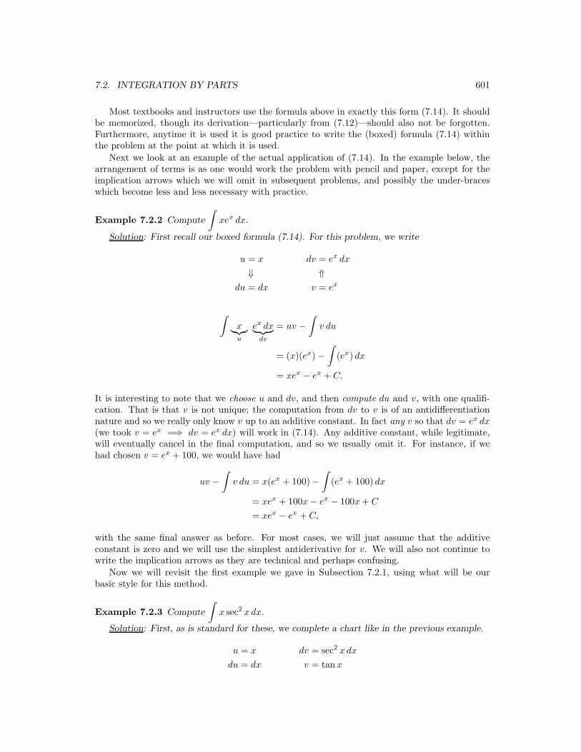
Example 7.2.2 Compute
∫
xex dx.
Solution: First recall our boxed formula (7.14). For this problem, we write
u = x dv = ex dx
⇓ ⇑du = dx v = ex
∫
x︸︷︷︸
u
ex dx︸ ︷︷ ︸
dv
= uv −∫
v du
= (x)(ex)−∫
(ex) dx
= xex − ex + C.
It is interesting to note that we choose u and dv, and then compute du and v, with one qualifi-cation. That is that v is not unique; the computation from dv to v is of an antidifferentiationnature and so we really only know v up to an additive constant. In fact any v so that dv = ex dx(we took v = ex =⇒ dv = ex dx) will work in (7.14). Any additive constant, while legitimate,will eventually cancel in the final computation, and so we usually omit it. For instance, if wehad chosen v = ex + 100, we would have had
uv −∫
v du = x(ex + 100)−∫
(ex + 100) dx
= xex + 100x− ex − 100x + C
= xex − ex + C,
with the same final answer as before. For most cases, we will just assume that the additiveconstant is zero and we will use the simplest antiderivative for v. We will also not continue towrite the implication arrows as they are technical and perhaps confusing.
Now we will revisit the first example we gave in Subsection 7.2.1, using what will be ourbasic style for this method.
Example 7.2.3 Compute
∫
x sec2 xdx.
Solution: First, as is standard for these, we complete a chart like in the previous example.
u = x dv = sec2 xdx
du = dx v = tanx

602 CHAPTER 7. ADVANCED INTEGRATION TECHNIQUES
∫
x sec2 xdx =
∫
u dv
= uv −∫
v du
= x tan x−∫
tanxdx
= x tan x− ln | secx|+ C.
Since this method is more complicated than substitution, there are more complicated consid-erations in how to apply it. First of course, one should attempt an earlier, simpler method. Butif those fail, and integration by parts is to be attempted,5 the following guidelines for choosingu and dv should be considered for our formula
∫u dv = uv −
∫v du:
1. u and dv must account for all factors of the original integral, and no more.
1.5. Of course, dv must contain the differential term (for example, dx) as a factor, butcan contain more terms.
2. v =∫
dv should be computable with relative ease.
3. du = u′(x) dx (assuming the original integral was in x) should not be overly complicated.
4. The integral∫
v du should be simpler than the original integral∫
u dv.6
The next example illustrates the importance of consideration 2 above.
Example 7.2.4 Compute
∫
x3 sinx2 dx.
Solution: We do not want to make u = sin x2, because then dv = x3 dx, giving du = 2x cosx2
and v = 14x4, and our
∫v du will be
∫12x5 cosx2 dx, which is worse than our original integral.
We will instead take u to be some power of x, but not all of x3, else the terms remaining fordv would be dv = sin x2 dx, which we cannot integrate with ordinary methods.7
What we will settle on is dv = x sin x2 dx, because its integral is an easy substitution we canshort-cut as in Section 7.1. We leave the remaining terms, collectively x2, for u:
u = x2 dv = x sin x2 dx
du = 2xdx v = −1
2cosx2
5Of course with practice one can see ahead whether or not integration by parts is likely to achieve an answerfor a particular integral.
6Later, in a twist on the method, we will see that the we do not requireR
v du be easier than the original,R
u dv, in all cases, but it is desirable in most cases.7In fact, we cannot compute
R
sinx2 dx using any kind of substitution or parts, or any other method of thistext for that matter, and arrive at an antiderivative in simple terms of the functions we know so far such aspowers, exponentials, logarithms, trigonometric or hyperbolic functions or their inverses. However, when westudy series we will find other expressions with which we can fashion an antiderivative of sin x2.
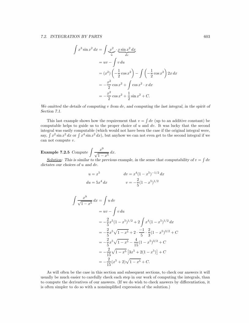
7.2. INTEGRATION BY PARTS 603
∫
x3 sin x2 dx =
∫
x2︸︷︷︸
u
·x sin x2 dx︸ ︷︷ ︸
dv
= uv −∫
v du
= (x2)
(
−1
2cosx2
)
−∫ (
−1
2cosx2
)
2xdx
= −x2
2cosx2 +
∫
cosx2 · xdx
= −x2
2cosx2 +
1
2sin x2 + C.
We omitted the details of computing v from dv, and computing the last integral, in the spirit ofSection 7.1.
This last example shows how the requirement that v =∫
dv (up to an additive constant) becomputable helps to guide us to the proper choice of u and dv. It was lucky that the secondintegral was easily computable (which would not have been the case if the original integral were,say,
∫x2 sin x2 dx or
∫x4 sin x2 dx), but anyhow we can not even get to the second integral if we
can not compute v.
Example 7.2.5 Compute
∫x9
√1− x5
dx.
Solution: This is similar to the previous example, in the sense that computability of v =∫
dvdictates our choices of u and dv.
u = x5 dv = x4(1− x5)−1/2 dx
du = 5x4 dx v = −2
5(1 − x5)1/2
∫x9
√1− x5
dx =
∫
u dv
= uv −∫
v du
= −2
5x5(1− x5)1/2 + 2
∫
x4(1− x5)1/2 dx
= −2
5x5
√
1− x5 + 2 · −1
5· 23(1− x5)3/2 + C
= −2
5x5
√
1− x5 − 4
15(1− x5)3/2 + C
= − 2
15
√
1− x5[3x5 + 2(1− x5)
]+ C
= − 2
15(x5 + 2)
√
1− x5 + C.
As will often be the case in this section and subsequent sections, to check our answers it willusually be much easier to carefully check each step in our work of computing the integrals, thanto compute the derivatives of our answers. (If we do wish to check answers by differentiation, itis often simpler to do so with a nonsimplified expression of the solution.)

604 CHAPTER 7. ADVANCED INTEGRATION TECHNIQUES
7.2.3 Repeated Use of Integration by Parts
The next examples show a different lesson: that it is sometimes appropriate to integrate by partsmore than once in a given problem. At each step, the hope is that the integral
∫v du is simpler
than the integral it came from (∫
u dv) in the integration by parts formula. Sometimes the newintegral
∫v du is indeed simpler, but not so much so that it can be integrated readily. Indeed,
at times that second integral also needs integration by parts, and so on, until we arrive at anintegral that we can compute easily.
Example 7.2.6 Compute
∫
x2 cos 3xdx.
Solution: The x2 term is complicating our integral, and so we reduce its effect somewhat byan integration by parts step.
u = x2 dv = cos 3xdx
du = 2xdx v =1
3sin 3x
∫
x2cos 3xdx = uv −∫
v du
=1
3x2 sin 3x−
∫2
3x sin 3xdx.
(7.15)
While we still cannot compute this last integral directly with old methods, it is better than theoriginal in the sense that our trigonometric function is multiplied by a first-degree polynomial,where in the original the polynomial was second-degree. One more application of integration byparts and there will be no polynomial factor at all in the new integral.
A strict use of the language would force us to introduce two new variables other than u andv, but since they have “disappeared” in the present form of our answer, namely 1
3x2 sin 3x −23
∫x sin 3xdx, it is not considered such bad form to “reset” (or “recycle”) u and v for another
integration by parts step, this time involving the integral∫
x sin 3xdx:
u = x dv = sin 3xdx
du = dx v = −1
3cos 3x
∫
x sin 3xdx = uv −∫
v du
= −x
3cos 3x +
1
3
∫
cos 3xdx
= −x
3cos 3x +
1
3· 13
sin 3x + C1.
Now we insert this last result into our original computation (7.15):
∫
x2 cos 3xdx =x2
3sin 3x− 2
3
[
−x
3cos 3x +
1
9sin 3x + C1
]
=x2
3sin 3x +
2
9x cos 3x− 2
27sin 3x + C.
7.2. INTEGRATION BY PARTS 605
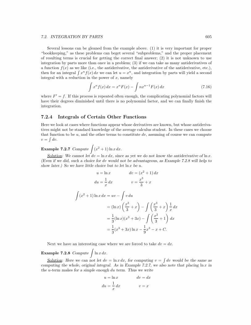
Several lessons can be gleaned from the example above. (1) it is very important for proper“bookkeeping,” as these problems can beget several “subproblems,” and the proper placementof resulting terms is crucial for getting the correct final answer; (2) it is not unknown to useintegration by parts more than once in a problem; (3) if we can take as many antiderivatives ofa function f(x) as we like (i.e., the antiderivative, the antiderivative of the antiderivative, etc.),then for an integral
∫xnf(x) dx we can let u = xn, and integration by parts will yield a second
integral with a reduction in the power of x, namely∫
xnf(x) dx = xnF (x)−∫
nxn−1F (x) dx (7.16)
where F ′ = f . If this process is repeated often enough, the complicating polynomial factors willhave their degrees diminished until there is no polynomial factor, and we can finally finish theintegration.
7.2.4 Integrals of Certain Other Functions
Here we look at cases where functions appear whose derivatives are known, but whose antideriva-tives might not be standard knowledge of the average calculus student. In these cases we choosethat function to be u, and the other terms to constitute dv, assuming of course we can computev =
∫dv.
Example 7.2.7 Compute
∫
(x2 + 1) lnxdx.
Solution: We cannot let dv = lnxdx, since as yet we do not know the antiderivative of lnx.(Even if we did, such a choice for dv would not be advantageous, as Example 7.2.8 will help toshow later.) So we have little choice but to let lnx be u.
u = lnx dv = (x2 + 1) dx
du =1
xdx v =
x3
3+ x
∫
(x2 + 1) lnxdx = uv −∫
v du
= (lnx)
(x3
3+ x
)
−∫ (
x3
3+ x
)1
xdx
=1
3(lnx)(x3 + 3x)−
∫ (x2
3+ 1
)
dx
=1
3(x3 + 3x) lnx− 1
9x3 − x + C.
Next we have an interesting case where we are forced to take dv = dx.
Example 7.2.8 Compute
∫
lnxdx.
Solution: Here we can not let dv = lnxdx, for computing v =∫
dv would be the same ascomputing the whole, original integral. As in Example 7.2.7, we also note that placing lnx inthe u-term makes for a simple enough du term. Thus we write
u = lnx dv = dx
du =1
xdx v = x
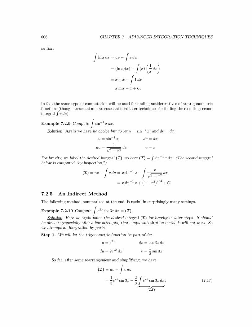
606 CHAPTER 7. ADVANCED INTEGRATION TECHNIQUES
so that∫
lnxdx = uv −∫
v du
= (lnx)(x) −∫
(x)
(1
xdx
)
= x lnx−∫
1 dx
= x lnx− x + C.
In fact the same type of computation will be used for finding antiderivatives of arctrigonometricfunctions (though arcsecant and arccosecant need later techniques for finding the resulting secondintegral
∫v du).
Example 7.2.9 Compute
∫
sin−1 xdx.
Solution: Again we have no choice but to let u = sin−1 x, and dv = dx.
u = sin−1 x dv = dx
du =1√
1− x2dx v = x
For brevity, we label the desired integral (I), so here (I) =∫
sin−1 xdx. (The second integralbelow is computed “by inspection.”)
(I) = uv −∫
v du = x sin−1 x−∫
x√1− x2
dx
= x sin−1 x +(1− x2
)1/2+ C.
7.2.5 An Indirect Method
The following method, summarized at the end, is useful in surprisingly many settings.
Example 7.2.10 Compute
∫
e2x cos 3xdx = (I).
Solution: Here we again name the desired integral (I) for brevity in later steps. It shouldbe obvious (especially after a few attempts) that simple substitution methods will not work. Sowe attempt an integration by parts.
Step 1. We will let the trigonometric function be part of dv:
u = e2x dv = cos 3xdx
du = 2e2x dx v =1
3sin 3x
So far, after some rearrangement and simplifying, we have
(I) = uv −∫
v du
=1
3e2x sin 3x− 2
3
∫
e2x sin 3xdx
︸ ︷︷ ︸
(II)
. (7.17)

7.2. INTEGRATION BY PARTS 607
This does not seem any easier than the first integral, so perhaps we might continue, but thistime let the trigonometric function be u and the exponential (along with dx) be containedin dv.
Step 2–First Attempt. Compute (II) =∫
e2x sin 3xdx in light of the comments at the endof the first step.
u = sin 3x dv = e2x dx
du = 3 cos 3xdx v =1
2e2x
(II) = uv −∫
v du =1
2e2x sin 3x− 3
2
∫
e2x cos 3xdx.
Combining this with the conclusion (7.17) of Step 1 gives us:
(I) =1
3e2x sin 3x− 2
3
[1
2e2x sin 3x− 3
2
∫
e2x cos 3xdx
]
=1
3e2x sin 3x− 1
3e2x sin 3x +
∫
e2x cos 3xdx
=
∫
e2x cos 3xdx.
Unfortunately that puts us right back where we started. However, a minor change in our effortabove will eventually lead us to the solution. While keeping Step 1, our next step towards asolution is to replace Step 2 by the same strategy as used in Step 1, namely that we use theexponential function for u and the trigonometric function in the dv term.
Step 2—Second Attempt. Again we attempt to compute (II) =∫
e2x sin 3xdx, thoughwith different choices of u and dv.
u = e2x dv = sin 3xdx
du = 2e2x dx v = −1
3cos 3x
(II) = uv −∫
v du
= −1
3e2x cos 3x +
2
3
∫
e2x cos 3xdx. (7.18)
It may seem that (7.18) is also a dead end, since it contains the original integral. But thisattempt is different. In fact, when we combine (7.18) with (7.17) we get
(I) =1
3e2x sin 3x− 2
3(II)
=1
3e2x sin 3x− 2
3
[
−1
3e2x cos 3x +
2
3
∫
e2x cos 3xdx
]
=1
3e2x sin 3x +
2
9e2x cos 3x− 4
9
∫
e2x cos 3xdx
︸ ︷︷ ︸
(I)
,
608 CHAPTER 7. ADVANCED INTEGRATION TECHNIQUES
which we can summarize by the following equation:
(I) =1
3e2x sin 3x +
2
9e2x cos 3x− 4
9(I). (7.19)
Now we are ready to derive (I), not by another calculus computation, but in fact by simplealgebra: we solve for it.
Step 3. Solve (7.19) for (I). First we add 49(I) to both sides of (7.19):
13
9(I) =
1
3e2x sin 3x +
2
9e2x cos 3x + C1. (7.20)
Here we include C1 because in fact each (I) in (7.19) represents all antiderivatives, whichdiffer from each other by additive constants. Now (7.19) made sense because of the factthat there are (hidden) additive constants on both sides of that equation (though on theright side they are multiplied by − 4
9 , but that still yields additive constants).8 Solving(7.20) for (I) we now have
(I) =9
13
[1
3e2x sin 3x +
2
9e2x cos 3x + C1
]
=3
13e2x sin 3x +
2
13e2x cos 3x + C, (7.21)
where C = 913C1.
Of course with this our original problem is solved:
∫
e2x cos 3xdx =3
13e2x sin 3x +
2
13e2x cos 3x + C.
What is important to understand about the example above is that sometimes, though wecannot perhaps directly compute a particular integral, it may happen that an indirect methodgives us the answer. Here we found an equation, namely (7.19), which our desired integralsatisfies, and for which (I) could be solved algebraically. We must be open to the possibility—indeed, the opportunity—of finding a desired quantity by such indirect methods, as well as directcomputations.
It should be pointed out that we could have computed the integral in Example 7.2.10 byinstead letting u be the trigonometric function, and dv = e2x dx in both Steps 1 and 2. In fact itis usually best to pick similar choices for u and dv when an integration by parts will take morethan one step. (Recall the discussion for
∫xnf(x) dx.)
The method of Example 7.2.10, namely solving for (I) after an integration by parts step, isavailable perhaps more often than one would think, though it is not a method of first resort.
The next example is also one in which we will eventually “solve” for the integral algebraically.
Example 7.2.11 Compute
∫
sin2 xdx = (I).
8In fact, two simultaneous appearances of (I) do not have to have the same additive constants, so (I)−(I) =C2, not zero.

7.2. INTEGRATION BY PARTS 609
Solution: The only reasonable choice here seems to be to let u = sin x and dv = sin dx, if weare to integrate this by parts.9
u = sin x dv = sin xdx
du = cosxdx v = − cosx
(I) =
∫
uv −∫
v du = − sin x cosx +
∫
cos2 xdx.
We could perform the same integration by parts with the second integral, which might or mightnot yield an equation we can solve for (I) (as the reader is invited to explore), but instead wewill use the fact that cos2 x = 1− sin2 x:
(I) = − sinx cosx +
∫
(1− sin2 x) dx
= − sinx cosx + x−∫
sin2 xdx
= x− sin x cos x− (I).
Adding (I) to both sides we get10
2(I) = − sinx cosx + x + C1
=⇒ (I) =1
2(x − sinx cos x) + C.
7.2.6 Miscellaneous Considerations
First we look at a definite integral arising from integration by parts. It should be pointed outthat the general formula will look like the following:11
∫ x=b
x=a
u dv = uv
∣∣∣∣
x=b
x=a
−∫ x=b
x=a
v du. (7.22)
9The integral in Example 7.2.11 can also be computed directly if we first use the trigonometric identitysin2 x = 1
2(1 − cos 2x), and then the identity sin 2x = 2 sin x cos x:
Z
sin2 x dx =
Z
1
2(1 − cos 2x) dx =
1
2x − 1
4sin 2x + C
=1
2x − 1
4· 2 sinx cos x + C =
1
2x − 1
2sin x cos x + C,
which is the same as the answer in the text of Example 7.2.11. In Section 7.3 we will opt for this alternativemethod, and indeed will make quite an effort to exploit the algebraic properties of the trigonometric functionswherever possible, but some integrals there will still require integration by parts.
10In fact many textbooks do not bother writing the C1 term, preferring to remind the student at the end thatan indefinite integral problem necessitates a “+C.”
11Some texts leave out the “x =” parts, assuming they are understood, but we will continue to use the conventionthat, unless otherwise stated, the “limits of integration” should correspond to values of the differential’s variable.Another popular way to write (7.22) avoids the issue:
Z
b
a
u(x)v′(x) dx = u(x)v(x)
˛
˛
˛
˛
b
a
−Z
b
a
v(x)u′(x) dx.

610 CHAPTER 7. ADVANCED INTEGRATION TECHNIQUES
Example 7.2.12 Compute
∫ π
−π
x sin xdx.
Solution: The antiderivative is an easier case than many of our previous examples, but carehas to be taken to keep track of all the signs (+/−) in computing the definite integral:
u = x dv = sin xdx
du = dx v = − cosx
∫ π
−π
x sin xdx = (−x cosx)∣∣π
−π+
∫ π
−π
cosxdx
= [−π cosπ]− [−(−π) cos(−π)] + sinx
∣∣∣∣
π
−π
= (−π)(−1)− (π)(−1) + sinπ − sin(−π)
= π + π + 0− 0
= 2π.
In the example above, we could also have noticed that∫ π
−πcosxdx is zero because we are
integrating over a whole period [−π, π] of cosx, and both sinx and cosx have definite integralzero over any full period [a, a + 2π]. (Think of their graphs, or their definite integrals over anysuch period.)
It is typical to compute that part u(x)v(x)∣∣b
aseparately, but one could instead separately
compute the entire antiderivative, and then evaluate at the two limits and take the difference:
∫ π
−π
x sin xdx = (−x cosx + sinx)
∣∣∣∣
π
−π
= (π + 0)− (−π + 0)
= 2π.
The choice of method is a matter of bookkeeping preferences, and perhaps whether or not part ofthe right-hand side of (7.22) is particularly simple. If not, it is reasonable to solve the indefiniteintegral
∫x sin xdx as a separate matter, and then write the definite integral with the formula
for the antiderivative inserted, as in∫
f(x) dx = F (x)∣∣b
aand so on as above.
The next example gives us several options for computing the new integral∫
v du along theway, though in each the original choices of u and dv are the same.
Example 7.2.13 Compute
∫
x tan−1 xdx = (I).
Solution: Again we have little choice on our selection of u and dv.
u = tan−1 x dv = xdx
du =1
x2 + 1dx v =
1
2x2
(I) = uv −∫
v du
=1
2x2 tan−1 x− 1
2
∫x2
x2 + 1dx.
7.2. INTEGRATION BY PARTS 611
Now this last integral can be found by first rewriting the integrand using either polynomial longdivision, or by using a little cleverness:
x2
x2 + 1=
x2 + 1− 1
x2 + 1=
x2 + 1
x2 + 1− 1
x2 + 1= 1− 1
x2 + 1.
Polynomial long division would have yielded the same result, and is a bit more straightforward,but the technique we used here is good to have available. Either way we then have
(I) =1
2x2 tan−1 x− 1
2
∫ (
1− 1
x2 + 1
)
dx
=1
2x2 tan−1 x− 1
2x +
1
2tan−1 x + C.
Though our choice of u and dv was limited, our choice of v was actually not as limited. Recallthat we could have chosen any v = 1
2x2 +C1. While previously we chose C1 = 0 for its apparentsimplicity, for this particular integral we could have actually saved ourselves some effort if wehad chosen v more strategically, with a different C1:
u = tan−1 x dv = xdx
du =1
x2 + 1dx v =
1
2
(x2 + 1
)
In effect we chose C1 = 12 . This gives us
(I) = uv −∫
v du
=1
2
(x2 + 1
)tan−1 x−
∫ 12 (x2 + 1)
x2 + 1dx
=1
2
(x2 + 1
)tan−1 x−
∫1
2dx
=1
2
(x2 + 1
)tan−1 x− 1
2x + C,
which is the same as before, though slightly rearranged.
Though rare, and not crucial, strategically adding a particular constant to the natural choicefor v can on occasion make for easier computations.
Integration by parts is a very important technique to have at one’s disposal when tacklingintegration problems. As has been demonstrated here, such problems can range from fairly simplecomputations which are perhaps just slightly more involved than more routine substitution-typeintegration problems, to some which utilize or indeed require much more clever applications ofthe technique. At the center of all these is a rearranged product rule,
u · dv
dx=
d(uv)
dx− v · du
dx,
which we can integrate to get∫
u · dv
dxdx =
∫d(uv)
dxdx−
∫
v · du
dxdx,
or our working formula which then follows:
∫
u dv = uv −∫
v du .
612 CHAPTER 7. ADVANCED INTEGRATION TECHNIQUES
Of course the applications can be quite clever and detailed, but they all are based upon thisrelatively simple formula.
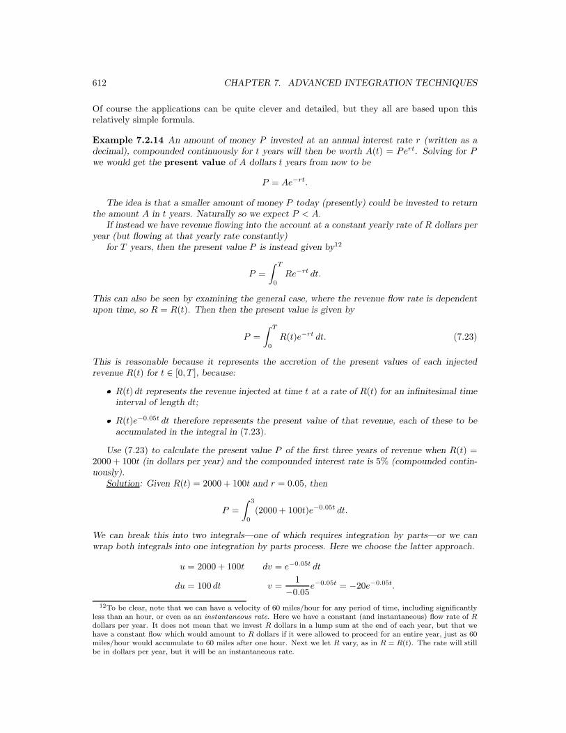
Example 7.2.14 An amount of money P invested at an annual interest rate r (written as adecimal), compounded continuously for t years will then be worth A(t) = Pert. Solving for Pwe would get the present value of A dollars t years from now to be
P = Ae−rt.
The idea is that a smaller amount of money P today (presently) could be invested to returnthe amount A in t years. Naturally so we expect P < A.
If instead we have revenue flowing into the account at a constant yearly rate of R dollars peryear (but flowing at that yearly rate constantly)
for T years, then the present value P is instead given by12
P =
∫ T
0
Re−rt dt.
This can also be seen by examining the general case, where the revenue flow rate is dependentupon time, so R = R(t). Then then the present value is given by
P =
∫ T
0
R(t)e−rt dt. (7.23)
This is reasonable because it represents the accretion of the present values of each injectedrevenue R(t) for t ∈ [0, T ], because:� R(t) dt represents the revenue injected at time t at a rate of R(t) for an infinitesimal time
interval of length dt;� R(t)e−0.05t dt therefore represents the present value of that revenue, each of these to beaccumulated in the integral in (7.23).
Use (7.23) to calculate the present value P of the first three years of revenue when R(t) =2000 + 100t (in dollars per year) and the compounded interest rate is 5% (compounded contin-uously).
Solution: Given R(t) = 2000 + 100t and r = 0.05, then
P =
∫ 3
0
(2000 + 100t)e−0.05t dt.
We can break this into two integrals—one of which requires integration by parts—or we canwrap both integrals into one integration by parts process. Here we choose the latter approach.
u = 2000 + 100t dv = e−0.05t dt
du = 100 dt v =1
−0.05e−0.05t = −20e−0.05t.
12To be clear, note that we can have a velocity of 60 miles/hour for any period of time, including significantlyless than an hour, or even as an instantaneous rate. Here we have a constant (and instantaneous) flow rate of Rdollars per year. It does not mean that we invest R dollars in a lump sum at the end of each year, but that wehave a constant flow which would amount to R dollars if it were allowed to proceed for an entire year, just as 60miles/hour would accumulate to 60 miles after one hour. Next we let R vary, as in R = R(t). The rate will stillbe in dollars per year, but it will be an instantaneous rate.

7.2. INTEGRATION BY PARTS 613
From this we get
P = (2000 + 100t)(−20e−0.05t
)∣∣∣∣
3
0
+
∫ 3
0
20e−0.05t · 100 dt
=
[
−2000(20 + t)e−0.05t +2000
−0.05e−0.05t
]∣∣∣∣
3
0
= (−80, 000− 2000t)e−0.05t
∣∣∣∣
3
0
= −80, 000e−0.15 + 80, 000e0 ≈ −74, 021 + 80, 000
=⇒ P ≈ 5, 979.
Ultimately, the computation in this example means that we would have to invest a lump sumof approximately $5979 at the same 5% (compounded continuously) rate today to accumulatethe total value of our more complicated investment strategy with a nonconstant revenue streamR(t) in the same three years (at the same interest rate), with that total being approximately (inpart because we have rounded to the nearest dollar for P ≈ $5979) A = 5979e0.05(3) ≈ 6947.
Another way to compute this total (future) value $6947 of our investment scheme after threeyears is to use the following computation (shown in general and for our specific case):
A(T ) =
∫ T
0
R(t)er(T−t) dt, A(3) =
∫ 3
0
(2000 + 100t) e0.05(3−t) dt. (7.24)
This is because we can look at the quantities inside the integral in the following way:� R(t) = (2000 + 100t) is the rate of revenue (investment) flowing into the account per unittime at time t.� R(t) dt = (2000 + 100t) dt represents the amount of new revenue invested during an in-finitesimal time interval of length dt at time t.� T − t = 3− t is the total length in years that the investment made at time t earns interest.
Thus the integral (7.24) represents the accretion of values of each injected revenue R(t) for alltimes t ∈ [0, T ]. For our case of R(t) = 2000+ 100t, r = 0.05 and [0, T ] = [0, 3] we integrate thisas before:
u = 2000 + 100t dv = e0.05(3−t) dt
du = 100 dt v = −20e0.05(3−t).
A(3) =
∫ 3
0
(2000 + 100t) e0.05(3−t) dt = − 20(2000 + 100t)e0.05(3−t)
∣∣∣∣
3
0
+ 2000
∫ 3
0
e0.05(3−t) dt
= − 20(2000 + 100t)e0.05(3−t)
∣∣∣∣
3
0
− 40, 000e0.05(3−t)
∣∣∣∣
3
0
= −80, 000(e0 − e.15
)− 6000
≈ 12, 947− 6000 = 6947,
so indeed we see that the value $6947 of the revenue stream in 3 years (calculated by (7.24)above) is the same as what our calculated present value P ≈ $5979 would be worth in 3 years ifinvested all at once now at the same 5% interest rate, compounded continuously.

614 CHAPTER 7. ADVANCED INTEGRATION TECHNIQUES
While in this model revenue R(t) is a continuous function approximating what in reality isa discrete depositing and interest phenomenon, we can nonetheless approximate (very well infact) with an integral what would be the present and future values of a somewhat complicatedrevenue injection and investment scheme, running for several years. This is one of many waysin which calculus is applied in business and economic settings.
Exercises
Compute the following integrals, all ofwhich can be computed “by parts.”
1.
∫
x sin xdx
2.
∫
x2 sin xdx
3.
∫
x cos 3xdx
4.
∫
x sec x tan xdx
5.
∫
x sec2 xdx
6.
∫
x lnxdx
7.
∫
x tan−1 xdx
8.
∫
x sec−1 xdx, x > 1
9.
∫
x sec−1 xdx, x < 1
10.
∫
x√
1− x dx. (Parts optional)
11.
∫x√
1− xdx (Parts optional)
12.
∫
xex dx
13.
∫
xex/2 dx
14.
∫
x3ex2
dx
15.
∫
x5 sin x3 dx
16.
∫
x2e3x dx
17.
∫
lnxdx
18.
∫
tan−1 xdx
19.
∫
sin−1 xdx
20.
∫
x√
1− x2 sin−1 x dx
21.
∫
x3 sin 2xdx
22.
∫
(lnx)2 dx
23.
∫
sin2 5xdx (Parts optional)
24.
∫
cos2 xdx (Parts optional)
25.
∫
e5x cos 2xdx
26.
∫
sec3 xdx
27. The current flowing in a particular cir-cuit as a function of time t is given byi = e−3t sin t. Determine the charge qwhich has passed through the circuit in[0, t]. Recall that i = dq
dt .
28. The slope of a curve is given bydy/dx = x3
√1 + x2. Find the equa-
tion of the curve if it passes throughthe point (0, 1).
7.2. INTEGRATION BY PARTS 615
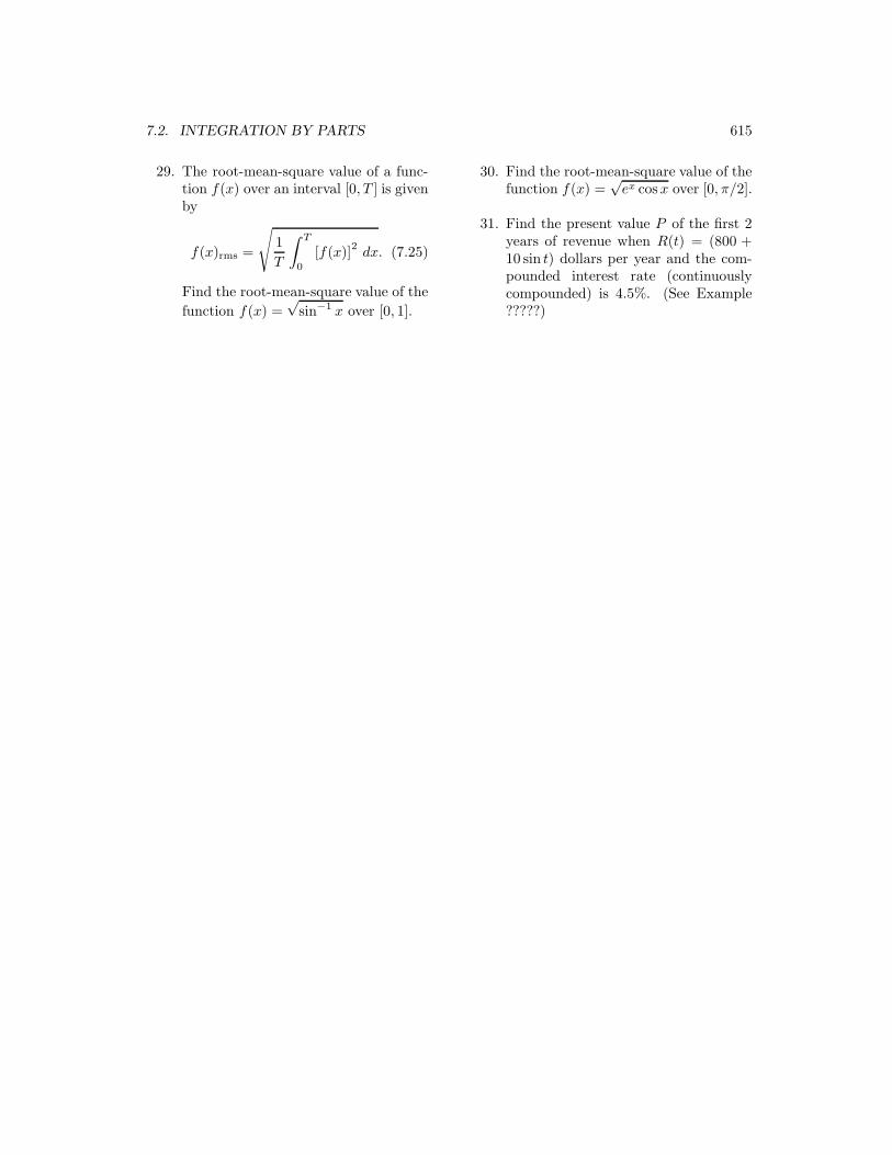
29. The root-mean-square value of a func-tion f(x) over an interval [0, T ] is givenby
f(x)rms =
√
1
T
∫ T
0
[f(x)]2
dx. (7.25)
Find the root-mean-square value of the
function f(x) =√
sin−1 x over [0, 1].
30. Find the root-mean-square value of thefunction f(x) =
√ex cosx over [0, π/2].
31. Find the present value P of the first 2years of revenue when R(t) = (800 +10 sin t) dollars per year and the com-pounded interest rate (continuouslycompounded) is 4.5%. (See Example?????)
616 CHAPTER 7. ADVANCED INTEGRATION TECHNIQUES
7.3 Trigonometric Integrals
We have already looked at two basic types of trigonometric integrals: those arising from thederivatives of the trigonometric functions (Subsection 6.1.4, page 532), and those of the elemen-tary substitution types in Section 6.5. In this section we are mainly interested in computingintegrals where the integrands are combinations of powers of trigonometric functions. In suchcases, the angles of each trigonometric function appearing are all the same. Another importanttopic considered here is how to deal with trigonometric combinations where the angles differ,and we will examine how to deal with several of those cases.
In the first examples where the angles agree, we rearrange the terms in the integrand and usethe three basic trigonometric identities to write the entire integral as function of one trigono-metric function, and its differential as the final factor. A substitution step then leads to one ormore power rules. Unfortunately this only leads to a solution if the combinations of powers areof a few simple forms. Still, these combinations occur often enough to warrant study.
After we look at those simplest forms, we look at other combinations of powers where theangles agree. Techniques include other algebraic manipulations, as well as integration by parts.
In the final forms, where the angles do not agree, we look at several trigonometric identitieswhich help us to rewrite the integrals into simpler forms.
7.3.1 Sample Problems
These first three examples illustrate an approach we develop in Subsections 7.3.2, 7.3.3 and 7.3.4.
Example 7.3.1 Compute
∫
tan2 xdx.
Solution:
∫
tan2 xdx =
∫
(sec2 x− 1) dx = tanx− x + C.
The example above used the facts that tan2 x = sec2 x− 1, and that we know the antiderivativeof sec2 x (where we might not have known the antiderivative of tan2 x immediately). The integralabove does not in itself contain a general method. Indeed there is no general method, but thereare ways to rewrite many trigonometric integrals to make their computations more elementary.
Example 7.3.2 Compute
∫
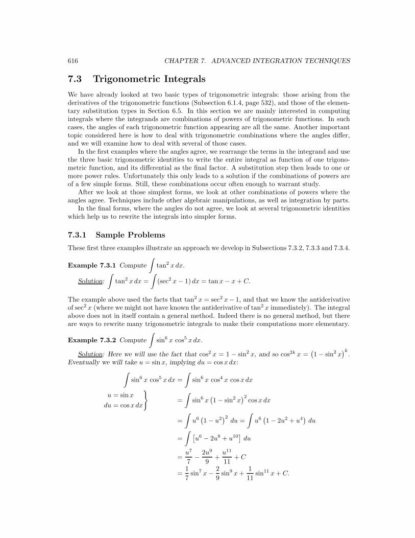
sin6 x cos5 xdx.
Solution: Here we will use the fact that cos2 x = 1 − sin2 x, and so cos2k x =(1− sin2 x
)k.
Eventually we will take u = sin x, implying du = cosxdx:∫
sin6 x cos5 xdx =
∫
sin6 x cos4 x cosxdx
u = sin x
du = cosxdx
}
=
∫
sin6 x(1− sin2 x
)2cosxdx
=
∫
u6(1− u2
)2du =
∫
u6(1− 2u2 + u4
)du
=
∫[u6 − 2u8 + u10
]du
=u7
7− 2u9
9+
u11
11+ C
=1
7sin7 x− 2
9sin9 x +
1
11sin11 x + C.

7.3. TRIGONOMETRIC INTEGRALS 617
Example 7.3.3 Compute
∫
sec5 x tan3 xdx.
Solution: Here we will borrow a factor of secant, and another of tangent, to form the func-tional part of du, where u = sec x:
∫
sec5 x tan3 xdx =
∫
sec4 x tan2 x sec x tan xdx
=
∫
sec4 x(sec2 x− 1
)sec x tan xdx
=
∫
u4(u2 − 1
)du
=
∫[u6 − u4
]du
=u7
7− u5
5+ C
=1
7sec7 x− 1
5sec5 x + C.
Now we look at these three specific techniques more closely and generalize them.
7.3.2 Odd Powers of Sine or Cosine
Here we are interested in the cases of integrals∫
sinm θ cosn θ dθ. (7.26)
where either m or n is odd. Suppose, for example, that m is odd, so that we can write m = 2k+1for some integer k. Then we rewrite the form (7.26) as
∫
sinm θ cos2k+1 θ dθ =
∫
sinm θ cos2k θ cos θ dθ.
The cos θ term which we “peeled away” becomes the functional part of the du, where u = sin θ(so du = cos θ dθ). We then write the rest of the integral in terms of u = sin θ. To do so we use
sin2 θ + cos2 θ = 0
⇐⇒ cos2 θ = 1− sin2 θ
=⇒ cos2k θ =(1− sin2 θ
)k.
Using this fact in the integral above, and setting u = sin θ, we get∫
sinm θ cos2k+1 θ dθ =
∫
sinm θ cos2k θ cos θ dθ
=
∫
sinm θ(1− sin2 θ
)kcos θ dθ
=
∫
um(1− u2
)kdu.
This yields a polynomial integrand, which we may then wish to expand before computing (witha sequence of power rules).

618 CHAPTER 7. ADVANCED INTEGRATION TECHNIQUES
Similarly, if there is an odd power of the sine, we can use the fact that sin2 θ = 1 − cos2 θ,and eventually using u = cos θ, to rewrite such an integral
∫
sin2k+1 θ cos θ dθ =
∫
sin2k θ cos θ sin θ dθ
=
∫(1− cos2 θ
)kcosn θ sin θ dθ
=
∫(1− u2
)kun(−du)
= −∫
(1− u2
)kun du.
In both of these it was crucial that we had an odd number of factors of either the sine orcosine, since “peeling off” one factor then leaves an even number, which can be easily writtenin terms of the other trigonometric function. The peeled off factor is then the functional part ofthe differential after substitution.
Note that while any even power of a sine or cosine function can be written entirely in termsof the other, this is not the case with odd powers.13 This technique works because removing afactor from an odd power of sine or cosine, both provides the functional part of du and leaves aneven power, which we write in terms of the other function which is then u in the substitution.
Example 7.3.4 Compute
∫
sin5 x cos4 xdx.
Solution: Here we see an odd number of sine factors, as so we peel one away to be part ofthe differential term, and write the entire integral in terms of the cosine:
∫
sin5 x cos4 xdx =
∫
sin4 x cos4 x sin xdx
=
∫(sin2 x
)2cos4 x sin xdx
=
∫(1− cos2 x
)2cos4 x sin xdx.
(In most future computations we will skip the second line above.) Now we take
u = cosx
=⇒ du = − sinxdx
⇐⇒ −du = sin xdx.
With the substitution we will have a polynomial to integrate. To summarize and finish the
13Consider the trigonometric identity sin2 θ + cos2 θ = 1. When solved for either the sine or cosine function,we get one of the following:
sin θ = ±p
1 − cos2 θ,
cos θ = ±p
1 − sin2 θ.
We see the ambiguity in the ±, and the introduction of a radical which itself can very much complicate an integral.However, when we raise these to even powers the radicals and the ± both disappear, and we are left with sumsof nonnegative, integer powers.

7.3. TRIGONOMETRIC INTEGRALS 619
problem, we have:∫
sin5 x cos4 xdx =
∫(1− cos2 x
)2cos4 x sinxdx
=
∫(1− u2
)2u4(−du)
= −∫
(1− 2u2 + u4
)u4 du
= −∫
(u4 − 2u6 + u8
)du
= −1
5u5 +
2
7u7 − 1
9u9 + C
= −1
5cos5 x +
2
7cos7 x− 1
9cos9 x + C.
It should be clear that one can not easily differentiate the final answer and immediatelyrecognize the original integrand. This is because some trigonometric identities were used to getan integrand form which was computable using these methods. Indeed, it is best to check thevalidity of the steps from the beginning, rather than to differentiate a tentative answer. However,it is an interesting exercise—left to the interested reader—in trigonometric identities to performthe differentiation, and then validate that the answer there is the original integrand.
It is not necessary that the angle is always x. However, for this technique we do require theangles inside the trigonometric functions to always match, and for the approximate differentialof the variable of substitution to be present.
Example 7.3.5 Compute
∫
sin4 5x cos3 5xdx.
Solution: Here there is an odd number of cosine terms, and we act accordingly.∫
sin4 5x cos3 5xdx =
∫
sin4 5x cos2 5x cos 5xdx
=
∫
sin4 5x(1− sin2 5x
)cos 5xdx.
Here we have
u = sin 5x
=⇒ du = 5 cos 5xdx
⇐⇒ 1
5du = cos 5xdx.
Now we begin again, incorporating this new information into our computation:∫
sin4 5x cos3 5xdx =
∫
sin4 5x(1− sin2 5x
)cos 5xdx
=
∫
u4(1− u2
)· 15
du
=1
5
∫(u4 − u6
)du
=1
5· 15
u5 − 1
5· 17
u7 + C
=1
25sin5 5x− 1
35sin7 5x + C.
620 CHAPTER 7. ADVANCED INTEGRATION TECHNIQUES
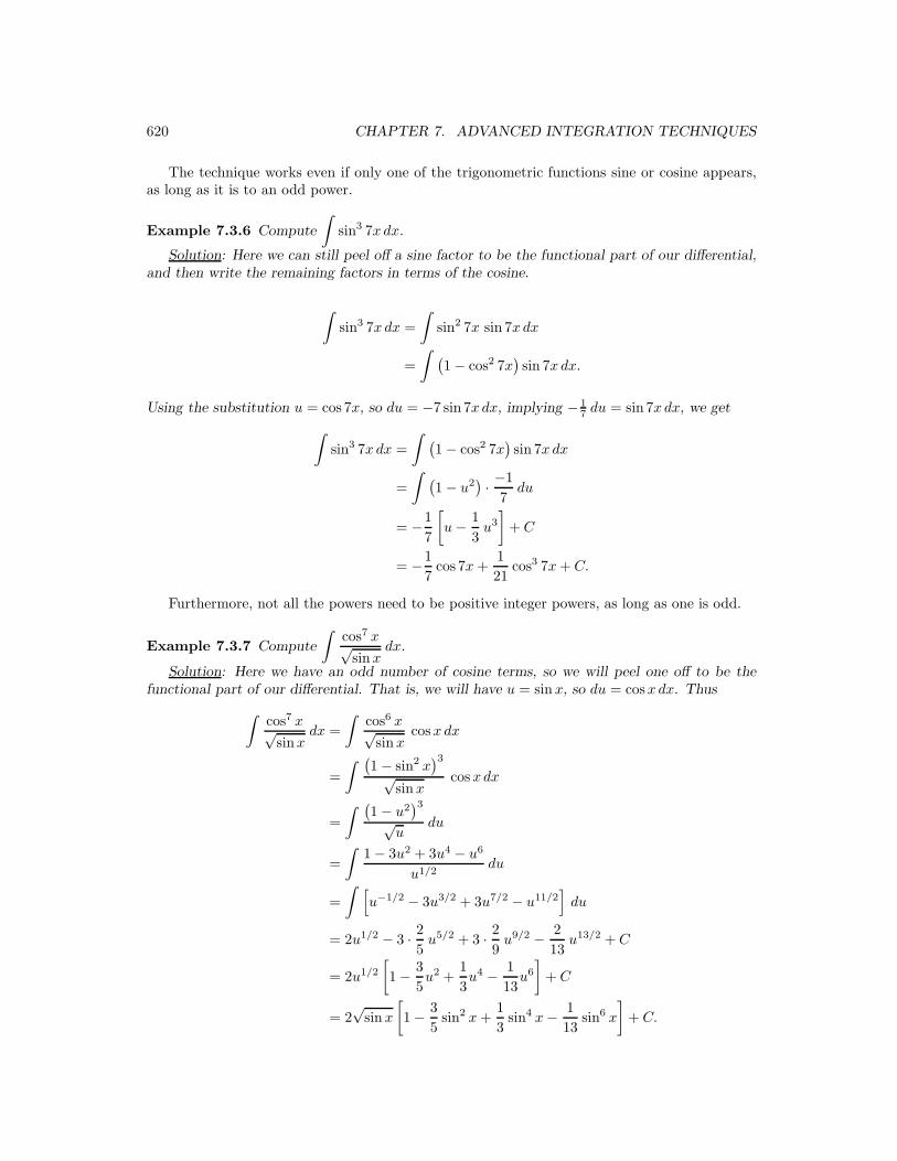
The technique works even if only one of the trigonometric functions sine or cosine appears,as long as it is to an odd power.
Example 7.3.6 Compute
∫
sin3 7xdx.
Solution: Here we can still peel off a sine factor to be the functional part of our differential,and then write the remaining factors in terms of the cosine.
∫
sin3 7xdx =
∫
sin2 7x sin 7xdx
=
∫(1− cos2 7x
)sin 7xdx.
Using the substitution u = cos 7x, so du = −7 sin 7xdx, implying − 17 du = sin 7xdx, we get
∫
sin3 7xdx =
∫(1− cos2 7x
)sin 7xdx
=
∫(1− u2
)· −1
7du
= −1
7
[
u− 1
3u3
]
+ C
= −1
7cos 7x +
1
21cos3 7x + C.
Furthermore, not all the powers need to be positive integer powers, as long as one is odd.
Example 7.3.7 Compute
∫cos7 x√
sin xdx.
Solution: Here we have an odd number of cosine terms, so we will peel one off to be thefunctional part of our differential. That is, we will have u = sin x, so du = cosxdx. Thus
∫cos7 x√
sinxdx =
∫cos6 x√
sin xcosxdx
=
∫ (1− sin2 x
)3
√sin x
cosxdx
=
∫ (1− u2
)3
√u
du
=
∫1− 3u2 + 3u4 − u6
u1/2du
=
∫ [
u−1/2 − 3u3/2 + 3u7/2 − u11/2]
du
= 2u1/2 − 3 · 25
u5/2 + 3 · 29
u9/2 − 2
13u13/2 + C
= 2u1/2
[
1− 3
5u2 +
1
3u4 − 1
13u6
]
+ C
= 2√
sin x
[
1− 3
5sin2 x +
1
3sin4 x− 1
13sin6 x
]
+ C.
7.3. TRIGONOMETRIC INTEGRALS 621
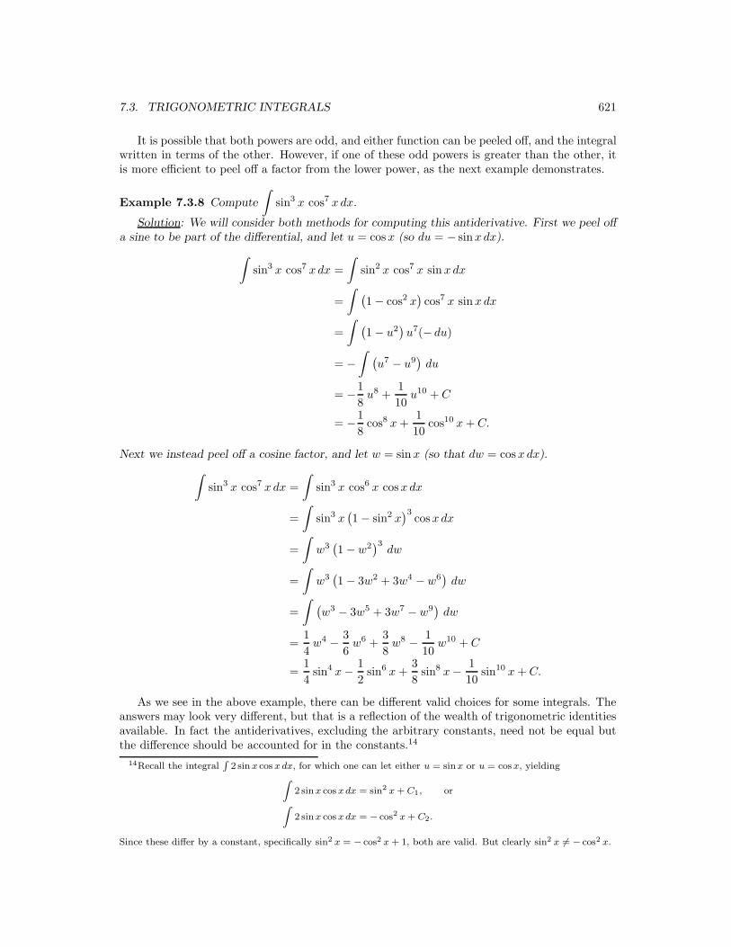
It is possible that both powers are odd, and either function can be peeled off, and the integralwritten in terms of the other. However, if one of these odd powers is greater than the other, itis more efficient to peel off a factor from the lower power, as the next example demonstrates.
Example 7.3.8 Compute
∫
sin3 x cos7 xdx.
Solution: We will consider both methods for computing this antiderivative. First we peel offa sine to be part of the differential, and let u = cosx (so du = − sinxdx).
∫
sin3 x cos7 xdx =
∫
sin2 x cos7 x sin xdx
=
∫(1− cos2 x
)cos7 x sin xdx
=
∫(1− u2
)u7(− du)
= −∫
(u7 − u9
)du
= −1
8u8 +
1
10u10 + C
= −1
8cos8 x +
1
10cos10 x + C.
Next we instead peel off a cosine factor, and let w = sin x (so that dw = cosxdx).
∫
sin3 x cos7 xdx =
∫
sin3 x cos6 x cosxdx
=
∫
sin3 x(1− sin2 x
)3cosxdx
=
∫
w3(1− w2
)3dw
=
∫
w3(1− 3w2 + 3w4 − w6
)dw
=
∫(w3 − 3w5 + 3w7 − w9
)dw
=1
4w4 − 3
6w6 +
3
8w8 − 1
10w10 + C
=1
4sin4 x− 1
2sin6 x +
3
8sin8 x− 1
10sin10 x + C.
As we see in the above example, there can be different valid choices for some integrals. Theanswers may look very different, but that is a reflection of the wealth of trigonometric identitiesavailable. In fact the antiderivatives, excluding the arbitrary constants, need not be equal butthe difference should be accounted for in the constants.14
14Recall the integralR
2 sin x cos x dx, for which one can let either u = sinx or u = cos x, yieldingZ
2 sinx cos x dx = sin2 x + C1, or
Z
2 sinx cos x dx = − cos2 x + C2.
Since these differ by a constant, specifically sin2 x = − cos2 x + 1, both are valid. But clearly sin2 x 6= − cos2 x.
622 CHAPTER 7. ADVANCED INTEGRATION TECHNIQUES
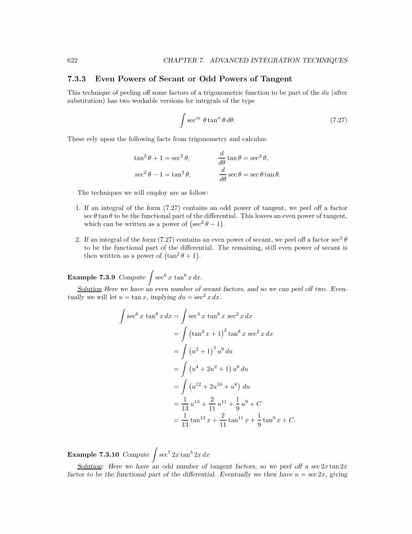
7.3.3 Even Powers of Secant or Odd Powers of Tangent
This technique of peeling off some factors of a trigonometric function to be part of the du (aftersubstitution) has two workable versions for integrals of the type
∫
secm θ tann θ dθ. (7.27)
These rely upon the following facts from trigonometry and calculus:
tan2 θ + 1 = sec2 θ,d
dθtan θ = sec2 θ,
sec2 θ − 1 = tan2 θ,d
dθsec θ = sec θ tan θ.
The techniques we will employ are as follow:
1. If an integral of the form (7.27) contains an odd power of tangent, we peel off a factorsec θ tan θ to be the functional part of the differential. This leaves an even power of tangent,which can be written as a power of
(sec2 θ − 1
).
2. If an integral of the form (7.27) contains an even power of secant, we peel off a factor sec2 θto be the functional part of the differential. The remaining, still even power of secant isthen written as a power of
(tan2 θ + 1
).
Example 7.3.9 Compute
∫
sec6 x tan8 xdx.
Solution Here we have an even number of secant factors, and so we can peel off two. Even-tually we will let u = tanx, implying du = sec2 xdx.
∫
sec6 x tan8 xdx =
∫
sec4 x tan8 x sec2 xdx
=
∫(tan2 x + 1
)2tan8 x sec2 xdx
=
∫(u2 + 1
)2u8 du
=
∫(u4 + 2u2 + 1
)u8 du
=
∫(u12 + 2u10 + u8
)du
=1
13u13 +
2
11u11 +
1
9u9 + C
=1
13tan13 x +
2
11tan11 x +
1
9tan9 x + C.
Example 7.3.10 Compute
∫
sec7 2x tan5 2xdx
Solution: Here we have an odd number of tangent factors, so we peel off a sec 2x tan 2xfactor to be the functional part of the differential. Eventually we then have u = sec 2x, giving

7.3. TRIGONOMETRIC INTEGRALS 623
du = 2 sec 2x tan 2xdx and thus 12 du = sec 2x tan 2xdx.
∫
sec7 2x tan5 2xdx =
∫
sec6 2x tan4 2x sec 2x tan 2xdx
=
∫
sec6 2x(sec2 2x− 1
)2sec 2x tan 2xdx
=
∫
u6(u2 − 1
)2 · 12
du
=1
2
∫
u6(u4 − 2u2 + 1
)du
=1
2
∫(u10 − 2u8 + u6
)du
=1
2
[1
11u11 − 2
9u9 +
1
7u7
]
+ C
=1
22sec11 2x− 1
9sec9 2x +
1
14sec7 2x + C.
In fact this last example could be computed by first rewriting the integral in terms of cosinesand sines:
∫sin5 2x
cos12 2xdx =
∫sin4 2x
cos12 2xsin 2xdx =
∫ (1− cos2 2x
)2
cos12 2xsin 2xdx
=
∫ (1− u2
)2
u12· −1
2du = −1
2
∫
u−12(1− 2u2 + u4
)du, etc.
Thus, the relationships involving the secant and tangent are not required in this last example.However, rewriting the integral in the previous problem, Example 7.3.9, in terms of sines andcosines would not yield an odd power of either. Thus Example 7.3.9 illustrates an integral whichdoes benefit from the extra structure (algebraic and calculus) of the secant-tangent relationship.
Example 7.3.11 Compute
∫
tan4 xdx.
Solution: Here we look at two solutions. In the first, instead of exploiting the fact that thereare an even number of factors of secant (namely zero) present here, we will repeatedly use thefact that tan2 θ + 1 = sec2 θ. (In the second line, we let u = tanx.)
∫
tan4 xdx =
∫
tan2 x(sec2 x− 1
)dx
=
∫
tan2 x︸ ︷︷ ︸
u2
sec2 x︸ ︷︷ ︸
du
dx−∫
tan2 xdx
=1
3tan3 x−
∫
tan2 xdx
=1
3tan3 x−
∫(sec2 x− 1
)dx
=1
3tan3 x− tan x + x + C.
Of course the other method is to “peel off” a factor of sec2 x, which we do even though it doesnot really appear. To have it appear, we will multiply and divide the integrand by sec2 x. Then

624 CHAPTER 7. ADVANCED INTEGRATION TECHNIQUES
we will let u = tanx. A long division will give us the sum of powers in our final integral below.15
∫
tan4 xdx =
∫tan4 x
sec2 xsec2 xdx
=
∫tan4 x
tan2 x + 1sec2 xdx
=
∫u4
u2 + 1du
=
∫ (
u2 − 1 +1
u2 + 1
)
du
=1
3u3 − u + tan−1 u + C1
=1
3tan3 x− tanx + tan−1(tanx) + C1
=1
3tan3 x− tanx + x + C.
Here we did have the extra complication of long division. Furthermore, to see that the twoanswers were the same we had to notice tan−1(tanx) = x + nπ, where n ∈ Z, i.e., n is aninteger. Thus the final constant C takes into account C1 − nπ, still a constant.
7.3.4 Even Powers of Cosecant or Odd Powers of Cotangent
Here we just point out that a similar relationship exists between the cosecant and cotangent, asexists between the secant and tangent. We briefly look at two examples to illustrate this. Theintegral type is
∫
cscm θ cotn θ dθ. (7.28)
We begin with the following facts from trigonometry and calculus:
cot2 θ + 1 = csc2 θ,d
dθcot θ = − csc2 θ,
csc2 θ − 1 = cot2 θ,d
dθcsc θ = − csc θ cot θ.
The techniques we will employ mirror those used for the secant-tangent integrals:
1. If an integral of the form (7.28) contains an odd power of cotangent, we peel off a fac-tor csc θ cot θ to be the functional part of the differential. This leaves an even power ofcotangent, which can be written as a power of
(csc2 θ − 1
).
2. If an integral of the form (7.28) contains an even power of cosecant, we peel off a factorcsc2 θ to be the functional part of the differential. The remaining even power of cosecantis then written as a power of
(cot2 θ + 1
).
15A clever student might also note that
u4
u2 + 1=
u4 − 1 + 1
u2 + 1=
u4 − 1
u2 + 1+
1
u2 + 1=
(u2 − 1)(u2 + 1)
u2 + 1+
1
u2 + 1= u2 − 1 +
1
u2 + 1.
However, such “clever” methods are difficult to generalize, and polynomial long division is more straightforward.

7.3. TRIGONOMETRIC INTEGRALS 625
Example 7.3.12 Compute
∫
csc8 x cot2 xdx.
Solution: We see an even number of cosecants, so we peel off two to be part of the differential.
∫
csc8 x cot2 xdx =
∫
csc6 x cot2 x csc2 xdx
=
∫(csc2 x
)3cot2 x csc2 xdx
=
∫(cot2 x + 1
)3cot2 x csc2 xdx.
Taking u = cotx, giving du = − csc2 xdx, so −du = csc2 xdx, we get
∫
csc8 x cot2 xdx
∫(cot2 x + 1
)3cot2 x csc2 xdx
=
∫(u2 + 1
)3u2(−du)
= −∫
(u6 + 3u4 + 3u2 + 1
)u2 du
= −∫
(u8 + 3u6 + 3u4 + u2
)du
= −1
9u9 − 3
7u7 − 3
5u5 − 1
3u3 + C
= −1
9cot9 x− 3
7cot7 x− 3
5cot5 x− 1
3cot3 x + C.
Example 7.3.13 Compute
∫
csc3 x
2cot3
x
2dx.
Solution: Here the cotangent appears to an odd power, so we will peel of one cosecant andone cotangent.
∫
csc3 x
2cot3
x
2dx =
∫
csc2 x
2cot2
x
2csc
x
2cot
x
2dx
=
∫
csc2 x
2
(
csc2 x
2− 1
)
cscx
2cot
x
2dx.
Now we let u = csc x2 , implying du = − csc x
2 cot x2 · 1
2 dx, whence −2 du = csc x2 cot x
2 dx. Ourintegral then becomes
∫
csc3 x
2cot3
x
2dx =
∫
csc2 x
2
(
csc2 x
2− 1
)
cscx
2cot
x
2dx
=
∫
u2(u2 − 1
)(−2) du
= −2
∫(u4 − u2
)du
= −2
5u5 +
2
3u3 + C
= −2
5csc5 x
2+
2
3csc3 x
2+ C.

626 CHAPTER 7. ADVANCED INTEGRATION TECHNIQUES
7.3.5 Even Powers of Sine and Cosine
Now we turn our attention to the question of integration when both powers of sine and cosine areeven. There are two standard methods for handling this: integration by parts, and “half-angleformulas.” The former is more useful when the powers are small than when they are large, andthe latter is perhaps more general.16
Example 7.3.14 Compute
∫
sin2 xdx using integration by parts.
Solution: This exact computation was performed in Example 7.2.11, page 609. So that it isin front of us here, we summarize that computation:
(I) =
∫
sin x︸︷︷︸
u
sin xdx︸ ︷︷ ︸
dv
= (sin x)︸ ︷︷ ︸
v
(− cosx)︸ ︷︷ ︸
v
−∫
(− cosx)︸ ︷︷ ︸
v
cosxdx︸ ︷︷ ︸
du
= − sin x cosx +
∫
cos2 xdx
= − sinx cos x +
∫(1− sin2 x
)dx = − sinx cosx + x−
∫
sin2 xdx
= x− sin x cosx− (I).
At this point we add (I) =∫
sin2 xdx to both sides to get
2
∫
sin2 xdx = x− sin x cosx + C1
=⇒∫
sin2 xdx =1
2(x− sin x cosx) + C.
The method above works well for integrating sin2 x or cos2 x, but higher, even powers becomemore cumbersome. For this reason it is common to opt for alternatives involving slightly moresophisticated trigonometric identities. There is some redundancy in the list below, as (7.29),(7.30), (7.31) and (7.33) together imply the others.
sin(−θ) = − sin θ, (7.29)
cos(−θ) = cos θ, (7.30)
sin(A + B) = sin A cosB + sin B cosA (7.31)
sin(A−B) = sin A cosB − sin B cosA (7.32)
cos(A + B) = cosA cosB − sin A sin B (7.33)
cos(A−B) = cosA cosB + sin A sin B (7.34)
sin 2θ = 2 sin θ cos θ (7.35)
cos 2θ = cos2 θ − sin2 θ (7.36)
cos 2θ = 2 cos2 θ − 1 (7.37)
cos 2θ = 1− 2 sin2 θ. (7.38)
It is left for the exercises to show that
1. Equation (7.32) follows from replacing B with −B in (7.31),
16In today’s calculus texts, integration by parts is less prominently presented for such integrals, while half-anglemethods are more popular among authors. We present both here for the lower powers, as some of the phenomenafound in the integration by parts for such integrals are found later in this section.

7.3. TRIGONOMETRIC INTEGRALS 627
2. Similarly, (7.34) follows from (7.33).
3. Equation (7.35) follows from (7.31), if we let A, B = θ.
4. Similarly (7.36) follows from (7.33).
5. (7.37) and (7.38) follow from (7.36) and the identity sin2 θ + cos2 θ = 1.
Now (7.37) and (7.38) can be rewritten as follow:
cos 2θ + 1 = 2 cos2 θ,
2 sin2 θ = 1− cos 2θ.
Dividing each of these by 2 gives us the so-called half-angle formulas:17
cos2 θ =1
2(1 + cos 2θ) , (7.39)
sin2 θ =1
2(1− cos 2θ) . (7.40)
Using (7.40), we see
∫
sin2 xdx =
∫1
2(1− cos 2x) dx =
1
2
[
x− 1
2sin 2x
]
+ C.
For reasons which will be clear in the next section, it is often desirable that the angle in the finalanswer agree with the original angle, in this case x. For that we use the double-angle formula(7.35), to get
∫
sin2 xdx =1
2
[
x− 1
2sin 2x
]
+ C =1
2
[
x− 1
2· 2 sinx cos x
]
+ C
=1
2x− 1
2sin x cosx + C.
This agrees with the answer we obtained through integration by parts, in Example 7.3.14,page 626.
Example 7.3.15 Compute
∫
sin4 xdx.
17Equations (7.39) and (7.40) are called half-angle formulas because the angle θ on the left is half of the angle2θ on the right. In fact, knowing the location of the terminal side of an angle does not tell us where its half islocated. Indeed, 90◦ and 450◦ are coterminal, but their half angles, 45◦ and 225◦ are not. This is reflected inwhat are given as “half-angle” formulas in most trigonometry texts (compare to (7.39) and (7.40)):
cosα
2= ±
r
1 + cos α
2
sinα
2= ±
r
1 − cos α
2.
However, knowing where an angle terminates does determine where twice the angle terminates, as is reflected in(7.35)–(7.38).

628 CHAPTER 7. ADVANCED INTEGRATION TECHNIQUES
Solution: Here we use the half-angle formulas repeatedly, until our integral has no positive,even powers of sine or cosine:
∫
sin4 xdx =
∫(sin2 x
)2dx =
∫ [1
2(1− cos 2x)
]2
dx
=1
4
∫(1− 2 cos 2x + cos2 2x
)dx
=1
4
∫ [
1− 2 cos 2x +1
2(1 + cos 4x)
]
dx
=1
4
∫ [3
2− 2 cos 2x +
1
2cos 4x
]
dx
=1
4
[3
2x− sin 2x +
1
2· 14
sin 4x
]
+ C
=3
8x− 1
4sin 2x +
1
32sin 4x + C.
This answer is correct, but if we want to match the angles to the original (x), we can use somedouble-angle formulas (7.35) and (7.36):
∫
sin4 xdx =3
8x− 1
4sin 2x +
1
32sin 4x + C
=3
8x− 1
4· 2 sinx cos x +
1
32· 2 sin 2x cos 2x + C
=3
8x− 1
2sin x cosx +
1
16(2 sinx cos x)(cos2 x− sin2 x) + C,
which can again be simplified and rewritten in several ways.
Example 7.3.16 Compute
∫
sin2 3x cos2 3xdx.
Solution:∫
sin2 3x cos2 3xdx =
∫1
2(1− cos 6x) · 1
2(1 + cos 6x) dx =
1
4
∫(1− cos2 6x
)dx
=1
4
∫ [
1− 1
2(1 + cos 12x)
]
dx =1
4
∫ [1
2− 1
2cos 12x
]
dx
=1
4
[x
2− 1
2· 1
12sin 12x
]
+ C =x
8− 1
96sin 12x + C.
(We could have used 1− cos2 6x = sin2 6x after the first line.) As before, if we would like to haveour answer in terms of the original angle, we need to utilize the double angle formulas (7.35)and (7.36):
∫
sin2 3x cos2 3xdx =x
8− 1
96sin 12x + C
=x
8− 1
96· 2 sin 6x cos 6x + C
=x
8− 1
48(2 sin 3x cos 3x)(cos2 3x− sin2 3x) + C
=x
8− 1
24sin 3x cos 3x(cos2 3x− sin2 3x) + C.

7.3. TRIGONOMETRIC INTEGRALS 629
Another method would be to have used the identity
sin θ cos θ =1
2sin 2θ, (7.41)
which follows quickly from the double-angle formula sin 2θ = 2 sin θ cos θ, i.e., (7.35). From thiswe can compute
∫
sin2 3x cos2 3xdx =
∫
(sin 3x cos 3x)2 dx
=
∫1
4sin2 6xdx
=1
4
∫1
2(1− cos 12x) dx
=1
8
(
x− 1
12sin 12x
)
+ C.
While the trigonometric parts of these antiderivatives look very different, the polynomial partsare all 1
8x. The trigonometric parts often take interesting manipulations via identities to verifythat they are the same, or off by an additive constant. The conclusion is that two studentsseeking antiderivatives of trigonometric functions may well have very different answers, thoughthe non-trigonometric parts are usually the same.
7.3.6 Miscellaneous Problems and Methods-I
There are many trigonometric integrals that either do not fit one of the above categories, or forwhich those methods are unwieldy. We will look at several such here. The reader should realize,however, that we cannot exhaust all possibilities here, and a particular problem may have aparticularly clever solution which does not generalize well to other problems.
The methods of the earlier subsections are all standard and any successful calculus studentis expected to know them. The first few examples here are of this class also, in that the betterstudents should be able to handle these without resorting to references. We will, however,eventually have methods in this subsection which such a student should be aware of, but isunderstandably less likely to be able to recite from memory. All are derivable, but again, thelatter are somewhat more obscure and even an excellent students might prefer to use a reference.It is important, however, that all students be aware of these latter classes of problems, and theavailable methods of solution, regardless of whether a reference is used ultimately.
Example 7.3.17 Compute
∫
sec3 xdx.
Solution: Here we have an odd number of secants, and an even (zero) number of tangents.Unfortunately our earlier methods called for an even number of secants or an odd number oftangents. We could notice that the integrand represents an odd number (−3) of cosines, andthen with u = sin x, we could write
∫
sec3 xdx =
∫1
cos3 xdx =
∫1
cos4 xcosxdx =
∫1
(1− sin2 x
)2 cosxdx =
∫1
(1− u2)2 du,
but in fact we have yet to discuss how to integrate that final form. (We will in Section 7.5, andwhile it will be somewhat long, it will be a straightforward computation there). Instead we will

630 CHAPTER 7. ADVANCED INTEGRATION TECHNIQUES
next try integration by parts. Since the integrand contains an easily integrated sec2 xdx factor,we will let that be dv:
u = secx dv = sec2 xdx
du = secx tan xdx v = tanx∫
sec3 xdx = uv −∫
v du = sec x tan x−∫
secx tan2 xdx.
Now it is tempting to do another parts step, with dv = sec x tan xdx, but—as happened in someprevious examples—we would then have our original integral on the left, and the same on theright (with all other functions cancelling). What works here is to instead use one of the basictrigonometric identities at this step:
∫
sec3 xdx = secx tan x−∫
secx tan2 xdx
= secx tan x−∫
secx(sec2 x− 1
)+ C
= secx tan x−∫
sec3 xdx +
∫
secxdx
= secx tan x + ln | secx + tanx| −∫
sec3 xdx.
Adding∫
sec3 xdx to both sides gives
2
∫
sec3 xdx = secx tan x + ln | sec x + tanx|+ C1
=⇒∫
sec3 xdx =1
2(sec x tan x + ln | secx + tanx|) + C.
When integrating arbitrary integer powers of the trigonometric functions, a common tech-nique is to make use of so-called reduction formulas. These are derived using integration byparts, often incorporating the kind of computation above. For instance, let us consider the gen-eral problem of integrating secn x, where n ≥ 3. Such an integral contains within its integrandthe factor sec2 x, which we use in the dv term. Integration by parts can proceed as follows:
u = secn−2 x dv = sec2 xdx
du = (n− 2) secn−3 x sec x · tan xdx v = tanx
i.e., du = (n− 2) secn−2 x tan xdx
giving us∫
secn xdx =
∫
secn−2 x︸ ︷︷ ︸
u
sec2 xdx︸ ︷︷ ︸
dv
= secn−2 x tan x−∫
(n− 2) secn−2 x tan2 xdx
= secn−2 x tan x−∫
(n− 2) secn−2 x(sec2 x− 1
)dx
= secn−2 x tan x− (n− 2)
∫
secn xdx + (n− 2)
∫
secn−2 xdx
=⇒ (n− 1)
∫
secn xdx = secn−2 x tan x + (n− 2)
∫
secn−2 xdx.
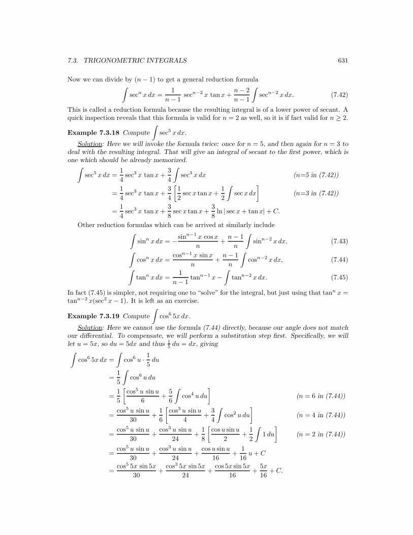
7.3. TRIGONOMETRIC INTEGRALS 631
Now we can divide by (n− 1) to get a general reduction formula∫
secn xdx =1
n− 1secn−2 x tan x +
n− 2
n− 1
∫
secn−2 xdx. (7.42)
This is called a reduction formula because the resulting integral is of a lower power of secant. Aquick inspection reveals that this formula is valid for n = 2 as well, so it is if fact valid for n ≥ 2.
Example 7.3.18 Compute
∫
sec5 xdx.
Solution: Here we will invoke the formula twice: once for n = 5, and then again for n = 3 todeal with the resulting integral. That will give an integral of secant to the first power, which isone which should be already memorized.
∫
sec5 xdx =1
4sec3 x tan x +
3
4
∫
sec3 xdx (n=5 in (7.42))
=1
4sec3 x tan x +
3
4
[1
2sec x tan x +
1
2
∫
secxdx
]
(n=3 in (7.42))
=1
4sec3 x tan x +
3
8sec x tan x +
3
8ln | secx + tanx|+ C.
Other reduction formulas which can be arrived at similarly include∫
sinn xdx = − sinn−1 x cosx
n+
n− 1
n
∫
sinn−2 xdx, (7.43)
∫
cosn xdx =cosn−1 x sin x
n+
n− 1
n
∫
cosn−2 xdx, (7.44)
∫
tann xdx =1
n− 1tann−1 x−
∫
tann−2 xdx. (7.45)
In fact (7.45) is simpler, not requiring one to “solve” for the integral, but just using that tann x =tann−2 x(sec2 x− 1). It is left as an exercise.
Example 7.3.19 Compute
∫
cos6 5xdx.
Solution: Here we cannot use the formula (7.44) directly, because our angle does not matchour differential. To compensate, we will perform a substitution step first. Specifically, we willlet u = 5x, so du = 5dx and thus 1
5 du = dx, giving∫
cos6 5xdx =
∫
cos6 u · 15
du
=1
5
∫
cos6 u du
=1
5
[cos5 u sin u
6+
5
6
∫
cos4 u du
]
(n = 6 in (7.44))
=cos5 u sin u
30+
1
6
[cos3 u sin u
4+
3
4
∫
cos2 u du
]
(n = 4 in (7.44))
=cos5 u sin u
30+
cos3 u sin u
24+
1
8
[cosu sinu
2+
1
2
∫
1 du
]
(n = 2 in (7.44))
=cos5 u sin u
30+
cos3 u sin u
24+
cosu sinu
16+
1
16u + C
=cos5 5x sin 5x
30+
cos3 5x sin 5x
24+
cos 5x sin 5x
16+
5x
16+ C.

632 CHAPTER 7. ADVANCED INTEGRATION TECHNIQUES
Clearly reduction formulas can be very useful. Indeed they provide an iterative methodfor reducing certain integral computations, step by step, until—hopefully—easily manageableintegrals appear. In fact in both examples above, we used the reduction formula for one morestep than necessary, because it was easier than recomputing
∫sec3 xdx or
∫cos2 u du as before.
Furthermore, many of the technical details for finding these integrals are built into the reductionformulas.
As useful as the reduction formulas are, they have a couple of minor drawbacks. First,when the angle does not match the differential, some substitution needs to be performed tocompensate. Second—and more serious—is that any attempt to memorize these is likely toresult in error. Thus the student of calculus needs to learn the earlier methods and be able toperform such calculations unaided, and also know that these reduction formulas (and others)are available and know how to use them.18
Now we consider integrals of following three forms, where m 6= n:∫
sinmx sin nxdx,
∫
sin mx cosnxdx,
∫
cosmx cosnxdx.
What distinguishes these is that the angles of the trigonometric functions do not agree. There aretwo methods for computing these: integration by parts, and utilizing the following trigonometricidentities:
sin A cosB =1
2[sin(A−B) + sin(A + B)] , (7.46)
sin A sin B =1
2[cos(A−B)− cos(A + B)] , (7.47)
cosA cosB =1
2[cos(A−B) + cos(A + B)] . (7.48)
For obvious reasons, these are called product-sum formulas. These follow from adding or sub-tracting (7.31), (7.32), (7.33), and (7.34), which we repeat here for reference:
sin(A + B) = sin A cosB + sin B cosA,
sin(A−B) = sin A cosB − sin B cosA,
cos(A + B) = cosA cosB − sinA sin B,
cos(A−B) = cosA cosB + sinA sin B.
For instance, (7.46) follows from adding the first two of these and solving for sinA cosB. Allthree, (7.46)–(7.48), are left to the exercises.
Example 7.3.20 Compute
∫
sin 2x cos 5xdx.
Solution: Here we use (7.46), with A = 2x and B = 5x:∫
sin 2x cos 5xdx =
∫1
2[sin(2x− 5x) + sin(2x + 5x)] dx
=
∫1
2[sin(−3x) + sin 7x] dx
=
∫1
2[− sin 3x + sin 7x] dx
=1
3cos 3x− 1
7cos 7x + C.
18Such formulas can be found in most engineering/science calculus texts, as well as books containing tables ofintegration formulas such as the CRC Standard Mathematical Tables and Formulae.

7.3. TRIGONOMETRIC INTEGRALS 633
The method above has the drawback that the solution does not contain the same angles asthe integrand. One can get back to the original angles using the formulas
cos 3x = cos(5x− 2x) = cos 5x cos 2x + sin 5x sin 2x,
cos 7x = cos(5x + 2x) = cos 5x cos 2x− sin 5x sin 2x.
Alternatively, an integration by parts argument leaves intact the angles. It requires two inte-gration by parts steps, and we need to solve for the integral. Furthermore, we have to make theanalogous substitution for u both times, and for dv both times. By analogous, here we meanusing the same angle, 2x or 5x, as the argument of the trigonometric function both times. Ifwe always let the u-term have angle 2x, and the dv-term have angle 5x, eventually the solutionthere will be
∫
sin 2x cos 5xdx =5
21sin 2x sin 5x +
2
21cos 2x cos 5x + C.
While it is far from obvious that these results are the same, it is an interesting exercise to checkthis last computation by computing the derivative of our answer here, so see how it simplifies tothe integrand.
7.3.7 Miscellaneous Problems and Methods-II
It is often the case that trigonometric integrals arise in the process of using another technique,and so the form of the integral may be more awkward than we have illustrated here so far. (Thiswill be the case particularly in Section 7.4.) In such cases it is often necessary to experimentwith rewriting the integral using whatever trigonometric identities apply. One also has to beaware that a substitution or integration-by-parts argument may be required eventually. Eventhen, if it is a multi-step application of integration by parts, it helps to recall when it helps tocontinue the “parts” step, and when it is better to use a trigonometric identity and solve for theintegral algebraically, as when we integrated sec3 x or csc3 x (see Example 7.3.17, completed onpage 630). In fact, once part of the process yields such an integral, it helps to know that such acomplication was probably inevitable and we might as well deal with it from there, rather thanattempt to bypass that problem.
With experience one learns to look ahead a few steps and anticipate which algebraic manipu-lation or identity will yield positive progress towards a form we can integrate (even if it requiressome cleverness such as needed to integrate sec3 x), but it is not uncommon to require multi-ple attempts to integrate a trigonometric integral before finding a strategy that will ultimatelysucceed.
Example 7.3.21 Compute
∫
tan2 θ sec θ dθ.
Solution: We will attempt to compute this integral two different methods. First we willintegrate by parts, noting that
∫
tan2 θ sec θ dθ =
∫
tan θ · sec θ tan θ dθ.
u = tan θ dv = sec θ tan θ dθ
du = sec2 θ dθ v = sec θ

634 CHAPTER 7. ADVANCED INTEGRATION TECHNIQUES
∫
tan2 θ sec θ dθ =
∫
tan θ︸ ︷︷ ︸
u
sec θ tan θ dθ︸ ︷︷ ︸
dv
= tan θ sec θ︸ ︷︷ ︸
uv
−∫
sec θ︸︷︷︸
v
sec2 θ dθ︸ ︷︷ ︸
du
= sec θ tan θ −∫
sec3 θ dθ
= sec θ tan θ −∫
sec2 θ sec θ dθ
= sec θ tan θ −∫
[(tan2 θ + 1
)sec θ
]dθ
= sec θ tan θ −∫
tan2 θ sec θ dθ −∫
sec θ dθ
= sec θ tan θ −∫
tan2 θ sec θ dθ − ln | sec θ + tan θ|+ C1
=⇒ 2
∫
tan2 θ sec θ dθ = secθ tan θ − ln | sec θ + tan θ|+ C1
=⇒∫
tan2 θ sec θ dθ =1
2sec θ tan θ − 1
2ln | sec θ + tan θ|+ C.
Because an intermediate step included the integral of sec3 θ, which by itself would require anintegration by parts technique that includes solving for the integral, it was likely that part of thesolution would include our original integral on the left. Rather than beginning an integration byparts, the simple experiment of rewriting sec3 θ as sec2 θ sec θ, and ultimately (tan2 θ + 1) sec θ,was successful in producing a form in which we could solve for our original integral.
The other method of attack is to write the entire integral in terms of sec x in the first place:
∫
tan2 x sec xdx =
∫
(sec2 x− 1) secxdx
=
∫
(sec3 x− secx) dx.
While the second function in the integral has a standard and known antiderivative, as mentionedearlier there seems to be no way to avoid integrating sec3 x or similarly complicated terms, so forit we then either use a reduction formula or integrate by parts, using the indirect method wherewe solve for the integral. The latter approach was built into our first (successful) approach inthis example.
Alternatively we could have computed∫
sec3 θ dθ elsewhere and inserted the computationhere. That computation could have been carried out as before (Example 7.3.17), or through theappropriate reduction formula (7.42), page 631.
The next example can be computed in two ways, but the first that we show here in factrequires a technique from a later section, namely Section 7.5. We show it here anyways inanticipation of the time when the student can call upon the ideas of more than one of thesesections for a single problem, as we did previously (in using integration by parts to solve atrigonometric integral, for instance).
Example 7.3.22 Compute
∫cos4 x
sin xdx.
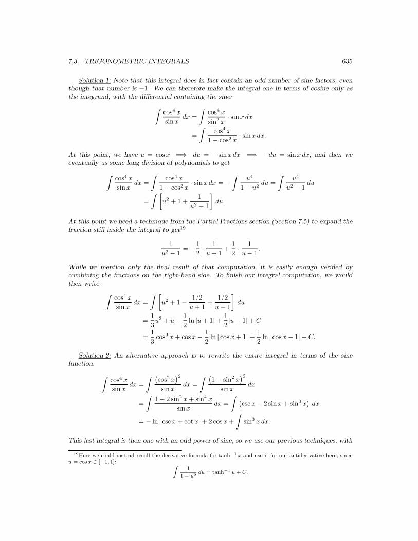
7.3. TRIGONOMETRIC INTEGRALS 635
Solution 1: Note that this integral does in fact contain an odd number of sine factors, eventhough that number is −1. We can therefore make the integral one in terms of cosine only asthe integrand, with the differential containing the sine:
∫cos4 x
sinxdx =
∫cos4 x
sin2 x· sinxdx
=
∫cos4 x
1− cos2 x· sinxdx.
At this point, we have u = cosx =⇒ du = − sinxdx =⇒ −du = sinxdx, and then weeventually us some long division of polynomials to get
∫cos4 x
sin xdx =
∫cos4 x
1− cos2 x· sin xdx = −
∫u4
1− u2du =
∫u4
u2 − 1du
=
∫ [
u2 + 1 +1
u2 − 1
]
du.
At this point we need a technique from the Partial Fractions section (Section 7.5) to expand thefraction still inside the integral to get19
1
u2 − 1= −1
2· 1
u + 1+
1
2· 1
u− 1.
While we mention only the final result of that computation, it is easily enough verified bycombining the fractions on the right-hand side. To finish our integral computation, we wouldthen write
∫cos4 x
sinxdx =
∫ [
u2 + 1− 1/2
u + 1+
1/2
u− 1
]
du
=1
3u3 + u− 1
2ln |u + 1|+ 1
2|u− 1|+ C
=1
3cos3 x + cosx− 1
2ln | cosx + 1|+ 1
2ln | cosx− 1|+ C.
Solution 2: An alternative approach is to rewrite the entire integral in terms of the sinefunction:
∫cos4 x
sin xdx =
∫ (cos2 x
)2
sin xdx =
∫ (1− sin2 x
)2
sin xdx
=
∫1− 2 sin2 x + sin4 x
sin xdx =
∫(cscx− 2 sinx + sin3 x
)dx
= − ln | cscx + cotx|+ 2 cosx +
∫
sin3 xdx.
This last integral is then one with an odd power of sine, so we use our previous techniques, with
19Here we could instead recall the derivative formula for tanh−1 x and use it for our antiderivative here, sinceu = cos x ∈ [−1, 1]:
Z
1
1 − u2du = tanh−1 u + C.
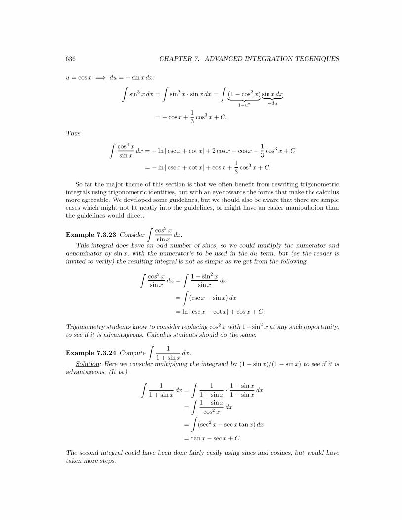
636 CHAPTER 7. ADVANCED INTEGRATION TECHNIQUES
u = cosx =⇒ du = − sinxdx:∫
sin3 xdx =
∫
sin2 x · sin xdx =
∫
(1− cos2 x)︸ ︷︷ ︸
1−u2
sinxdx︸ ︷︷ ︸
−du
= − cosx +1
3cos3 x + C.
Thus
∫cos4 x
sin xdx = − ln | cscx + cotx|+ 2 cosx− cosx +
1
3cos3 x + C
= − ln | cscx + cotx|+ cosx +1
3cos3 x + C.
So far the major theme of this section is that we often benefit from rewriting trigonometricintegrals using trigonometric identities, but with an eye towards the forms that make the calculusmore agreeable. We developed some guidelines, but we should also be aware that there are simplecases which might not fit neatly into the guidelines, or might have an easier manipulation thanthe guidelines would direct.
Example 7.3.23 Consider
∫cos2 x
sin xdx.
This integral does have an odd number of sines, so we could multiply the numerator anddenominator by sin x, with the numerator’s to be used in the du term, but (as the reader isinvited to verify) the resulting integral is not as simple as we get from the following.
∫cos2 x
sin xdx =
∫1− sin2 x
sinxdx
=
∫
(cscx− sin x) dx
= ln | cscx− cotx|+ cosx + C.
Trigonometry students know to consider replacing cos2 x with 1−sin2 x at any such opportunity,to see if it is advantageous. Calculus students should do the same.
Example 7.3.24 Compute
∫1
1 + sin xdx.
Solution: Here we consider multiplying the integrand by (1 − sin x)/(1− sin x) to see if it isadvantageous. (It is.)
∫1
1 + sin xdx =
∫1
1 + sinx· 1− sinx
1− sinxdx
=
∫1− sinx
cos2 xdx
=
∫
(sec2 x− secx tan x) dx
= tanx− sec x + C.
The second integral could have been done fairly easily using sines and cosines, but would havetaken more steps.
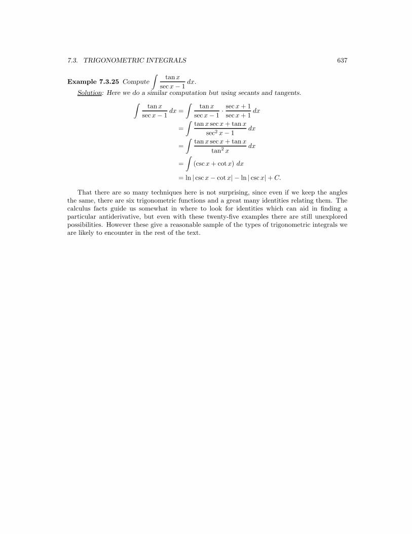
7.3. TRIGONOMETRIC INTEGRALS 637
Example 7.3.25 Compute
∫tanx
secx− 1dx.
Solution: Here we do a similar computation but using secants and tangents.
∫tan x
secx− 1dx =
∫tanx
secx− 1· secx + 1
secx + 1dx
=
∫tan x secx + tanx
sec2 x− 1dx
=
∫tan x secx + tanx
tan2 xdx
=
∫
(csc x + cotx) dx
= ln | cscx− cotx| − ln | cscx|+ C.
That there are so many techniques here is not surprising, since even if we keep the anglesthe same, there are six trigonometric functions and a great many identities relating them. Thecalculus facts guide us somewhat in where to look for identities which can aid in finding aparticular antiderivative, but even with these twenty-five examples there are still unexploredpossibilities. However these give a reasonable sample of the types of trigonometric integrals weare likely to encounter in the rest of the text.
638 CHAPTER 7. ADVANCED INTEGRATION TECHNIQUES
Exercises
Evaluate the following integrals.
1.
∫
sin x cosxdx
2.
∫
sin2 x cosxdx
3.
∫
sin x cos2 xdx
4.
∫
sin3 x cos2 xdx
5.
∫
sin4 x cos5 xdx
6.
∫sin3 x
cos2 xdx
7.
∫sin3 x
cos2 x + 1dx
8.
∫
sin4 x cos5 xdx
9.
∫
sin3 2x cos15 2xdx
10.
∫sin2 x
cosxdx
11.
∫
sin x ln | sin x| dx
12.
∫
cosx ln | sin x| dx
13. Prove (7.45), page 631.

7.4. TRIGONOMETRIC SUBSTITUTION 639
7.4 Trigonometric Substitution
In this section we explore how integrals can sometimes be solved by making some clever substi-tutions involving trigonometric functions, even though the original integrals themselves do notinvolve such functions.
7.4.1 Introduction
Before developing the general mechanics, we look at a few examples below for motivation.
Example 7.4.1 Compute
∫1√
1− x2dx, using a nontrivial substitution method.
Solution: We already know the answer to this integral, because we know ddx sin−1 x =
1/√
1− x2, so a “clever” but unnecessary substitution u = sin−1 x would yield the antiderivativequickly.20
But let us imagine for a moment that we do not have this antiderivative at our disposal, andneed to tackle this integral from first principles. Can we accomplish this without first developinga theory of derivatives of arc-trigonometric functions?
The answer is yes, if we are clever in a different way, which offers a more general method wecan apply to a class of more complicated integrals, as we will see. This substitution method isto notice that −1 < x < 1 is required in the integral, and that is nearly the same as the rangeof sin θ, namely −1 ≤ sin θ ≤ 1, and is in fact contained in it. So we make a substitution, albeitsomewhat “backwards” from what we are used to, where x will be a function of θ rather than afunction of x being explicitly some new variable:
∫1√
1− x2dx =
∫1
√
1− sin2 θcos θ dθ =
∫cos θ
cos θdθ =
∫
dθ = θ + C = sin−1 x + C
x = sin θ
=⇒ dx = cos θ dθ
∣∣∣∣∣
The above computation is completely correct, but there are a few technicalities to check.
1. Why are we allowed to take the nonnegative case above, when we know√
1− sin2 θ =√cos2 θ = | cos θ|? In other words, usually cos θ = ±
√
1− sin2 θ, but we took the “+”case.
2. Why can we automatically say x = sin θ =⇒ θ = sin−1 x? After all, there are infinitelymany angles with the same sine, and they need not necessarily even be coterminal whenwe graph them in standard position. (Example: sin π
4 = sin 3π4 = sin 9π
4 = sin 11π4, etc.)
The answer to both questions lies in the values for θ that we can choose when we make thesubstitution. In fact we were negligent by not fixing the range of θ from the outset, but we
20Anytime we know the antiderivative, we can perform a substitution where we define u to be that antiderivative,and the resulting integral will be
R
du = u + C, but this has relatively little use for discovery. For the integral inExample 7.4.1, we could have written
Z
1√1 − x2
dx =
Z
du = u + C = sin−1 x + C.
u = sin−1 x
=⇒ du =1
1 − x2dx
˛
˛
˛
˛
˛
˛

640 CHAPTER 7. ADVANCED INTEGRATION TECHNIQUES
will see there is a standard practice in which we will take exactly those angles θ (or a subsetof them) which are the same as the range of the relevant arc-trigonometric function. For theproblem above, it is assumed θ ∈
[−π
2 , π2
], since sin θ is one-to-one for these values, and sin θ
ranges over the whole range of the sine function for these values, i.e., for the same reason thearcsine is defined to output these values.
[−1, 1]︸ ︷︷ ︸
x∈
sin−1 x [
−π
2,π
2
]
︸ ︷︷ ︸
θ∈
[−1, 1]︸ ︷︷ ︸
x∈
sin θ
Thus we have mappings from x to θ and back. (When we actually compute the integral, weconcentrate on the second mapping more than the first, until we compute the antiderivative, inwhich case we may need the first mapping to “get back” to x.)
When we look at the values of θ and their terminal points on the unit circle, all doubt about
our casual computation√
1− sin2 θ =√
cos2 θ = | cos θ| = cos θ is laid to rest, because cosine isnonnegative in our range of angles θ:
1−1
1
−1
−π/2
π/2
(cos θ, sin θ)
θ
x = sin θ ≥ 0θ ∈ [0, π/2]cos θ ≥ 0
1−1
1
−1
−π/2
π/2
(cos θ, sin θ)
θ
x = sin θ ≤ 0θ ∈ [−π/2, 0]
cos θ ≥ 0
Now “x” here does not signify the coordinate on the horizontal axis. Indeed, for this particularcase “x” is the same as sin θ, which is the vertical (“y”) coordinate where our angle in standardposition (initial side being the positive horizontal axis) pierces the unit circle.
Note that having the angles θ ranging from −π/2 to π/2 means that −1 ≤ sin θ ≤ 1 is
equivalent to θ = sin−1 x, and also implies cos θ ≥ 0 and so cos θ =√
1− sin2 θ, where normally
we only have cos θ = ±√
1− sin2 θ:
1.(∀θ ∈
[−π2 , π
2
])[x = sin θ ←→ θ = sin−1 x], and
2.(∀θ ∈
[−π2 , π
2
]) [
cos θ =√
1− sin2 θ]
.
The example above illustrates another useful approach for some integrals:
1. Make a substitution to rewrite the integral in terms of an angle θ (with appropriate rangeof θ matching the range of values for x).
2. Compute the resultant trigonometric integral.
3. Rewrite the antiderivative in terms of x.

7.4. TRIGONOMETRIC SUBSTITUTION 641
Drawing diagrams on an appropriate circle as above will be quite useful in subsequent problems.The process can not only clarify somewhat our substitution process, but it can also allow us tocheck that we have correct signs for all the various cases for θ. Moreover, there are times whenwe need to read actual values of other trigonometric functions of θ, but in terms of x.
The process above may seem unnecessarily complicated, especially for an integral for which weknew the answer from the beginning. However, this advanced technique generalizes to integralswhich do not succumb to previous methods (though they should always be considered first!).For instance we would be hard-pressed to compute the antiderivative in the next example usingearlier techniques.
Example 7.4.2 Compute
∫ √1− x2
xdx.
Solution: Note first that this integral will not simply yield to earlier techniques. (The readeris welcome to try, to see where those methods eventually fall short.)
Note also that, due to the square root, we require −1 ≤ x ≤ 1. In fact we also cannot havex = 0, but that constraint will be consistent with our new integral upon substitution. Ultimatelyit is the radical which is giving us the most difficulty here.
The key to solving this problem is to again realize that [−1, 1] is exactly the range of thefunction sin θ, so we will again use the substitution x = sin θ in the integral above, with theunderstanding that θ ∈ [−π/2, π/2] (excluding zero due to the denominator). This time we willagain draw the diagram, but will label the various parts of the resulting triangles for futurereference. Note that in the second drawing, sin θ = x < 0 while cos θ =
√1− x2 is still a
positive quantity, and again, where the angle’s terminal ray pierces the unit circle is the point(cos θ, sin θ).
1−1
1
−1
−π/2
π/2
θx
1
√1− x2 1−1
1
−1
−π/2
π/2
θx
1
√1− x2
Note that we can now read all trigonometric functions of θ from the diagrams. For instance,tan θ = x/
√1− x2, regardless of which of the two quadrants contains the terminal ray of θ.
Now we perform the substitution, noting as usual that the differential must also be accountedfor:
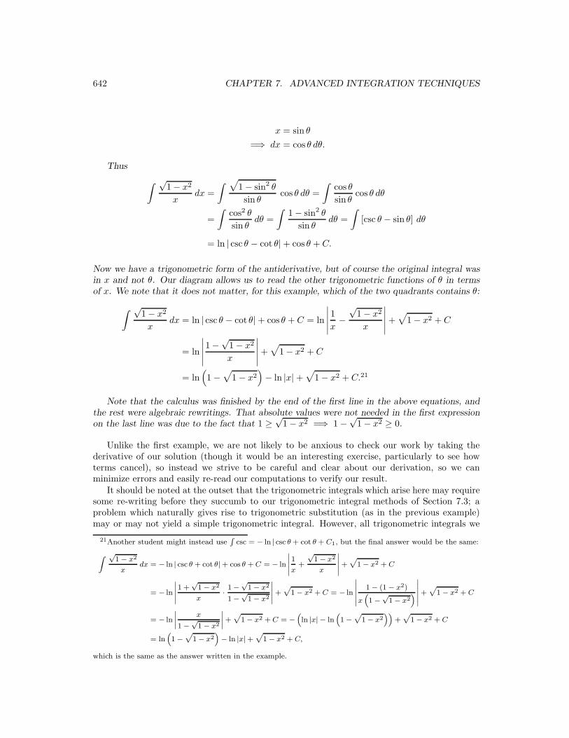
642 CHAPTER 7. ADVANCED INTEGRATION TECHNIQUES
x = sin θ
=⇒ dx = cos θ dθ.
Thus
∫ √1− x2
xdx =
∫ √
1− sin2 θ
sin θcos θ dθ =
∫cos θ
sin θcos θ dθ
=
∫cos2 θ
sin θdθ =
∫1− sin2 θ
sin θdθ =
∫
[csc θ − sin θ] dθ
= ln | csc θ − cot θ|+ cos θ + C.
Now we have a trigonometric form of the antiderivative, but of course the original integral wasin x and not θ. Our diagram allows us to read the other trigonometric functions of θ in termsof x. We note that it does not matter, for this example, which of the two quadrants contains θ:
∫ √1− x2
xdx = ln | csc θ − cot θ|+ cos θ + C = ln
∣∣∣∣∣
1
x−√
1− x2
x
∣∣∣∣∣+
√
1− x2 + C
= ln
∣∣∣∣∣
1−√
1− x2
x
∣∣∣∣∣+
√
1− x2 + C
= ln(
1−√
1− x2)
− ln |x|+√
1− x2 + C.21
Note that the calculus was finished by the end of the first line in the above equations, andthe rest were algebraic rewritings. That absolute values were not needed in the first expressionon the last line was due to the fact that 1 ≥
√1− x2 =⇒ 1−
√1− x2 ≥ 0.
Unlike the first example, we are not likely to be anxious to check our work by taking thederivative of our solution (though it would be an interesting exercise, particularly to see howterms cancel), so instead we strive to be careful and clear about our derivation, so we canminimize errors and easily re-read our computations to verify our result.
It should be noted at the outset that the trigonometric integrals which arise here may requiresome re-writing before they succumb to our trigonometric integral methods of Section 7.3; aproblem which naturally gives rise to trigonometric substitution (as in the previous example)may or may not yield a simple trigonometric integral. However, all trigonometric integrals we
21Another student might instead useR
csc = − ln | csc θ + cot θ + C1, but the final answer would be the same:
Z
√1 − x2
xdx = − ln | csc θ + cot θ| + cos θ + C = − ln
˛
˛
˛
˛
˛
1
x+
√1 − x2
x
˛
˛
˛
˛
˛
+p
1 − x2 + C
= − ln
˛
˛
˛
˛
˛
1 +√
1 − x2
x· 1 −
√1 − x2
1 −√
1 − x2
˛
˛
˛
˛
˛
+p
1 − x2 + C = − ln
˛
˛
˛
˛
˛
˛
1 − (1 − x2)
x“
1 −√
1 − x2”
˛
˛
˛
˛
˛
˛
+p
1 − x2 + C
= − ln
˛
˛
˛
˛
x
1 −√
1 − x2
˛
˛
˛
˛
+p
1 − x2 + C = −“
ln |x| − ln“
1 −p
1 − x2””
+p
1 − x2 + C
= ln“
1 −p
1 − x2”
− ln |x| +p
1 − x2 + C,
which is the same as the answer written in the example.

7.4. TRIGONOMETRIC SUBSTITUTION 643
will encounter here are of classes we considered in Section 7.3, so ultimately those techniquesequipped us for our work here.
Before we delve into other trigonometric substitutions, we will perform one more involvingthe sine.
Example 7.4.3 Compute
∫√
9− 25x2 dx.
Solution: As always, we should look to see if previous methods apply. They do not, withoutextraordinary cleverness, though it is interesting to note that simple substitution would work ifwe had an extra factor of x in the integrand. (We do not.)
Now in previous examples, we wanted to exploit the trigonometric identity 1−sin2 θ = cos2 θ.Here we will do the same, except we will multiply this equation by 9, giving us 9 − 9 sin2 θ =9 cos2 θ.
So we wish to have 25x2 = 9 sin2 θ, i.e., x2 = 925 sin2 θ. We get this if we let x = 3
5 sin θ.Below is what a student (or professor) might hand-write to compute this integral:
∫√
9− 25x2 dx =
∫ √
9− 25 · 9
25sin2 θ · 3
5cos θ dθ
25x2 = 9 sin2 θ
x2 =9
25sin2 θ
∴ Take x =3
5sin θ
=⇒ dx =3
5cos θ dθ
∣∣∣∣∣∣∣∣∣∣∣∣∣∣
=
∫ √
9− 9 sin2 θ · 35
cos θ dθ
=
∫ √
9(1− sin2 θ) · 35
cos θ dθ
=
∫
3√
1− sin2 θ · 35
cos θ dθ
=
∫9
5cos2 θ dθ
=
∫9
5· 12
(1 + cos 2θ) dθ
=9
10
(
θ +1
2sin 2θ
)
+ C
=9
10θ +
9
10· 12· 2 sin θ cos θ + C
=9
10θ +
9
10sin θ cos θ + C.
We require the final trigonometric antiderivative to be in terms of the angle θ (and not 2θ forexample), so that we can read the trigonometric functions of θ from the diagram. In constructingthe diagram, we need to solve our substitution for sin θ:
x =3
5sin θ =⇒ sin θ =
5x
3.
Note that our diagram below is not constructed on the unit circle, but on a more general circleof positive radius (in this case 3). As before, we have to consider both quadrants in which θ mayfall.

644 CHAPTER 7. ADVANCED INTEGRATION TECHNIQUES
θ
5x
3
√9− 25x2
0
π/2
θ 5x
3
√9− 25x2
0
−π/2
From these and our expression for sin θ above we can complete our integral computation:
∫√
9− 25x2 dx =9
10θ +
9
10sin θ cos θ + C
=9
10sin−1
(5x
3
)
+9
10· 5x
3·√
9− 25x2
3+ C
=9
10sin−1
(5x
3
)
+x
2
√
9− 25x2 + C.
7.4.2 The General Approach
There are cases where a different trigonometric substitution is appropriate and useful. In factthe choices are mutually exclusive, and the form to be used can be deduced from the range of x-values in the domain of the original integrand, though one instead usually sees how problematicterms would simplify. In the chart below, we use x, though “x” can be x or 5x, or similar, withthe necessary algebra and calculus to compensate. Also for simplicity, we assume a > 0:22
Integral contains:√
a2 − x2√
a2 + x2√
x2 − a2
Substitute: x = a sin θ x = a tan θ x = a sec θ
Motivation:√
a2 − x2 = a cos θ√
a2 + u2 = a sec θ√
x2 − a2 = a| tan θ|
Range of x: −a ≤ x ≤ a x ∈ R x ∈ (−∞,−a] ∪ [a,∞)Range of θ: θ ∈ [−π/2, π/2] θ ∈ (−π/2, π/2) θ ∈ [0, π/2) ∪ (π/2, π]
The graphs of the positions of θ are important for verification purposes, as well as for fillingin with x-expressions the trigonometric functions of θ that usually arise from the trigonometricform of the antiderivative.
22In fact, sometimes these substitutions are useful even when the radicals are not present, particularly forthe tangent case, such as in computing
R
1(x2+a2)n
dx. So we can perhaps make a general statement that these
substitutions should be considered if we have powers of (a2 − x2), (a2 + x2) or (a2 − x2), respectively, whenprevious methods will not work, and the range of values for x and θ are compatible.

7.4. TRIGONOMETRIC SUBSTITUTION 645
Example 7.4.4 Compute
∫1√
36 + x2dx.
Solution: Here we will let x = 6 tan θ. Note that as part of the method (but usually leftunstated), −π/2 < θ < π/2 ⇐⇒ −∞ < x <∞.
∫1√
36 + x2dx =
∫1√
36 + 36 tan2 θ· 6 sec2 θ dθ =
∫6 sec2 θ√36 sec2 θ
dθ =
∫6 sec2 θ
6 sec θdθ
x = 6 tan θ
=⇒ dx = 6 sec2 θ dθ
}
=
∫
sec θ dθ = ln | sec θ + tan θ|+ C1.
At this point we have the integral solved in terms of θ. To get back to x, we draw the relevanttriangles in which x = tan θ, i.e., tan θ = x/6. Note sec θ =
(√36 + x2
)/6 in both quadrants.
θ
x√ 36+
x2
60
π/2
θ x√36 +
x 2
60
−π/2
Thus∫
1√36 + x2
dx = ln | sec θ + tan θ|+ C1
= ln
∣∣∣∣∣
√36 + x2
6+
x
6
∣∣∣∣∣+ C1
= ln∣∣∣
√
36 + x2 + x∣∣∣− ln 6 + C1
= ln∣∣∣
√
36 + x2 + x∣∣∣ + C.
It is customary to have the solution in simplest possible form, which is why we expanded thelogarithm and absorbed the − ln 6 term into the constant. (One usually only puts the subscripton the C1 term after further lines reveal it is useful.)
As we see in the drawings of the relevant angles, when we use a tangent-type substitution weget the same, simple expressions for the derived sides regardless of which of the two quadrantsholds the terminal ray of θ. It is not always the case with the secant substitutions.
Example 7.4.5 Compute
∫√
x2 − 9 dx.
Solution: Here we let x = 3 sec θ.∫
√
x2 − 9 dx =
∫√
9 sec2 θ − 9 · 3 sec θ tan θ dθ
x = 3 sec θ
=⇒ dx = 3 sec θ tan θ dθ
}
=
∫ √
9 tan2 θ · 3 sec θ tan θ dθ
=
∫
3| tan θ| · 3 sec θ tan θ dθ
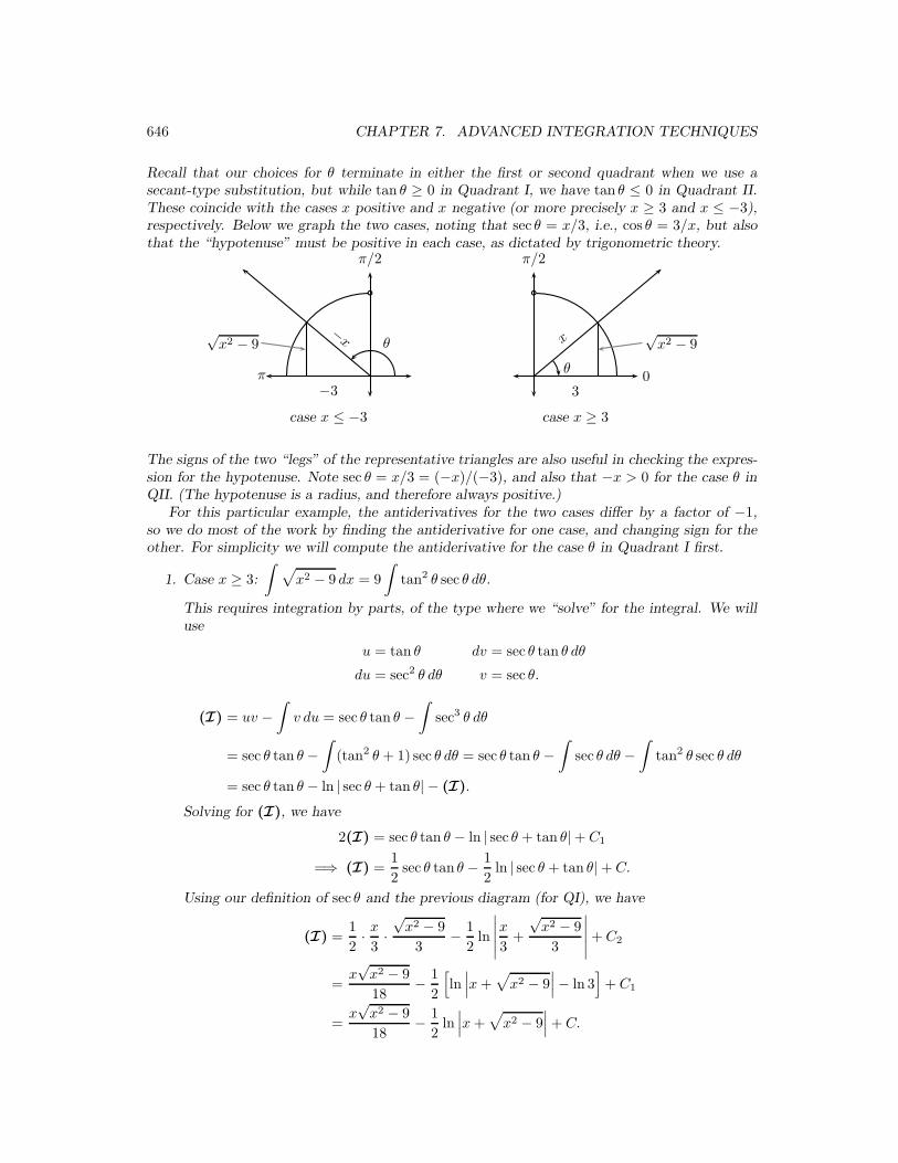
646 CHAPTER 7. ADVANCED INTEGRATION TECHNIQUES
Recall that our choices for θ terminate in either the first or second quadrant when we use asecant-type substitution, but while tan θ ≥ 0 in Quadrant I, we have tan θ ≤ 0 in Quadrant II.These coincide with the cases x positive and x negative (or more precisely x ≥ 3 and x ≤ −3),respectively. Below we graph the two cases, noting that sec θ = x/3, i.e., cos θ = 3/x, but alsothat the “hypotenuse” must be positive in each case, as dictated by trigonometric theory.
−x
−3
θ
π/2
π
case x ≤ −3
√x2 − 9
θ
√x2 − 9x
3
case x ≥ 3
0
π/2
The signs of the two “legs” of the representative triangles are also useful in checking the expres-sion for the hypotenuse. Note sec θ = x/3 = (−x)/(−3), and also that −x > 0 for the case θ inQII. (The hypotenuse is a radius, and therefore always positive.)
For this particular example, the antiderivatives for the two cases differ by a factor of −1,so we do most of the work by finding the antiderivative for one case, and changing sign for theother. For simplicity we will compute the antiderivative for the case θ in Quadrant I first.
1. Case x ≥ 3:
∫√
x2 − 9 dx = 9
∫
tan2 θ sec θ dθ.
This requires integration by parts, of the type where we “solve” for the integral. We willuse
u = tan θ dv = sec θ tan θ dθ
du = sec2 θ dθ v = sec θ.
(I) = uv −∫
v du = sec θ tan θ −∫
sec3 θ dθ
= sec θ tan θ −∫
(tan2 θ + 1) sec θ dθ = sec θ tan θ −∫
sec θ dθ −∫
tan2 θ sec θ dθ
= sec θ tan θ − ln | sec θ + tan θ| − (I).
Solving for (I), we have
2(I) = sec θ tan θ − ln | sec θ + tan θ|+ C1
=⇒ (I) =1
2sec θ tan θ − 1
2ln | sec θ + tan θ|+ C.
Using our definition of sec θ and the previous diagram (for QI), we have
(I) =1
2· x3·√
x2 − 9
3− 1
2ln
∣∣∣∣∣
x
3+
√x2 − 9
3
∣∣∣∣∣+ C2
=x√
x2 − 9
18− 1
2
[
ln∣∣∣x +
√
x2 − 9∣∣∣− ln 3
]
+ C1
=x√
x2 − 9
18− 1
2ln
∣∣∣x +
√
x2 − 9∣∣∣ + C.
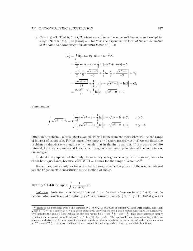
7.4. TRIGONOMETRIC SUBSTITUTION 647
2. Case x ≤ −3: That is, θ in QII, where we will have the same antiderivative in θ except fora sign. Here tan θ ≤ 0, so | tan θ| = − tan θ, so the trigonometric form of the antiderivativeis the same as above except for an extra factor of (−1):
(I) =
∫
3(− tan θ) · 3 sec θ tan θ dθ
=−1
2sec θ tan θ +
1
2ln | sec θ + tan θ|+ C
=−1
2· x3·√
x2 − 9
−3+
1
2ln
∣∣∣∣∣
x
3+
√x2 − 9
−3
∣∣∣∣∣+ C3
=x√
x2 − 9
18+
1
2
[
ln∣∣∣x−
√
x2 − 9∣∣∣− ln 3
]
+ C3
=x√
x2 − 9
18+
1
2ln
∣∣∣x−
√
x2 − 9∣∣∣ + C.
Summarizing,
∫√
x2 − 9 dx =
1
18x√
x2 − 9− 1
2ln
∣∣∣x +
√
x2 − 9∣∣∣ + C, x ≥ 3,
1
18x√
x2 − 9 +1
2ln
∣∣∣x−
√
x2 − 9∣∣∣ + C, x ≤ −3.
Often, in a problem like this latest example we will know from the start what will be the rangeof interest of values of x. For instance, if we know x ≥ 0 (more precisely, x ≥ 3) we can finish theproblem by drawing one diagram only, namely that in the first quadrant. If this were a definiteintegral, for instance, we would know which range of x we need by looking at the endpoints ofour integral.
It should be emphasized that only the secant-type trigonometric substitutions require us tocheck both quadrants, because
√sec2 θ − 1 = ± tan θ for the range of θ we use.23
Sometimes, particularly for tangent substitutions, no radical is present in the original integralyet the trigonometric substitution is the method of choice.
Example 7.4.6 Compute
∫1
(x2 + 9)2dx.
Solution: Note that this is very different from the case where we have (x2 + 9)1 in thedenominator, which would eventually yield a arctangent, namely 1
3 tan−1 x3 + C. But it gives us
23There is an approach where one assumes θ ∈ [0, π/2) ∪ [π, 3π/2) or similar QI and QIII angles, and then√sec2 θ − 1 = tan θ since tan θ ≥ 0 in those quadrants. However we avoid this because sometimes the antideriva-
tive includes the angle θ itself, which for our case would be θ = sec−1 x
3= cos−1 3
x. This other approach simply
redefines the arcsecant as well, so sec−1 z ∈ [0, π/2) ∪ [π,3π/2). The approach has many advantages (for in-stance the derivative of the arcsecant does not contain an absolute value), but at a cost of such conveniences assec−1 z = cos−1 1
z. One also redefines the arccosecant in that approach to arc-trigonometric functions.

648 CHAPTER 7. ADVANCED INTEGRATION TECHNIQUES
a hint of what to do, namely let x = 3 tan θ.
∫1
(x2 + 9)2dx =
∫1
(9 tan2 θ + 9
)2 · 3 sec2 θ dθ
x = 3 tan θ
dx = 3 sec2 θ dθ
} =
∫3 sec2 θ dθ
(9 sec2 θ)2
=
∫3 sec2 θ dθ
81 sec4 θ
=1
27
∫
cos2 θ dθ
=1
27· 12
∫
(1 + cos 2θ) dθ
=1
27
[1
2· θ +
1
2sin 2θ
]
+ C
=1
54θ +
1
27· 12· 2 sin θ cos θ + C.
Now the integral is solved in terms of θ, so we need to get back to x, which we again do by lookingat diagrams of the relation between x and θ, namely that tan θ = x/3, and θ ∈ (−π/2, π/2).
θ
x√ x2 +
9
30
π/2
θ x√x 2
+9
30
−π/2
Finishing off our integral is now fairly easy:
∫1
(x2 + 9)2dx =
1
54θ +
1
27· sin θ cos θ + C
=1
54tan−1 x +
1
27· x√
x2 + 9· 3√
x2 + 9+ C
=1
54tan−1 x +
1
9· x
x2 + 9+ C.
While this is a powerful approach, it is not always the technique of choice. For example,
∫x√
x2 − 9dx =
√
x2 − 9 + C,
from a simple substitution, or perhaps even an anticipation of the general form followed by acheck of multiplicative constants. Similarly, if we replaced x with x2 in the numerator we couldintegrate by parts. If we found ourselves integrating by parts twice, for instance (perhaps itis x3 in the numerator) it may well be more efficient to use trigonometric substitution, or anintegration by parts step may ultimately require it! But trigonometric substitution is usuallynot the method of choice if previous methods apply.

7.4. TRIGONOMETRIC SUBSTITUTION 649
Example 7.4.7 Compute
∫ √x2 − 5
xdx assuming that x ≥
√5.
Solution: Here we let x2 = 5 sec2 θ, i.e., x =√
5 sec θ, giving dx =√
5 sec θ tan θ dθ. Notethat we are assuming positive x, so θ ∈ [0, π/2) so θ terminates in QI, where tan θ ≥ 0. Thus,
∫ √x2 − 5
xdx =
∫ √5 sec2 θ − 5√
5 sec θ·√
5 sec θ tan θ dθ
=
∫ √5 tan θ√5 sec θ
·√
5 sec θ tan θ dθ
=√
5
∫
tan2 θ dθ
=√
5
∫(sec2 θ − 1
)dθ
=√
5 tan θ −√
5θ + C
=√
5 ·√
x2 − 5√5−√
5 sec−1 x√5
+ C
=√
x2 − 5 + sec−1 x√5
+ C.
θ
√x2 − 5x
√5
0
π/2
Exercises
1. Use trigonometric substitution to de-rive the general formula (a > 0)
∫dx√
a2 − x2= sin−1 x
a+ C.
2. Use trigonometric substitution to de-rive the general formula (a > 0)
∫dx
a2 + x2=
x
atan−1 x
a+ C.
3. Use trigonometric substitution to de-rive the general formula for x > a > 0:
∫dx
x√
x2 − a2=
x
asec−1 x
a+ C.
4. Compute
∫ √1− x2
x2dx.
5. Compute
∫(9− x2
)3/2dx.
6. Compute
∫1
(25 + 9x2)5/2dx.
7. Compute
∫√
x2 + 2xdx. (Complete
the square.)
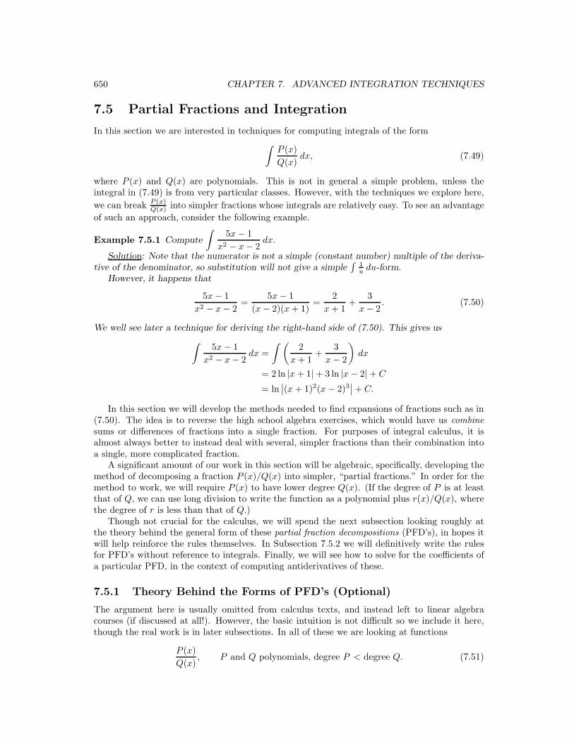
650 CHAPTER 7. ADVANCED INTEGRATION TECHNIQUES
7.5 Partial Fractions and Integration
In this section we are interested in techniques for computing integrals of the form
∫P (x)
Q(x)dx, (7.49)
where P (x) and Q(x) are polynomials. This is not in general a simple problem, unless theintegral in (7.49) is from very particular classes. However, with the techniques we explore here,
we can break P (x)Q(x) into simpler fractions whose integrals are relatively easy. To see an advantage
of such an approach, consider the following example.
Example 7.5.1 Compute
∫5x− 1
x2 − x− 2dx.
Solution: Note that the numerator is not a simple (constant number) multiple of the deriva-tive of the denominator, so substitution will not give a simple
∫1u du-form.
However, it happens that
5x− 1
x2 − x− 2=
5x− 1
(x− 2)(x + 1)=
2
x + 1+
3
x− 2. (7.50)
We well see later a technique for deriving the right-hand side of (7.50). This gives us
∫5x− 1
x2 − x− 2dx =
∫ (2
x + 1+
3
x− 2
)
dx
= 2 ln |x + 1|+ 3 ln |x− 2|+ C
= ln∣∣(x + 1)2(x− 2)3
∣∣ + C.
In this section we will develop the methods needed to find expansions of fractions such as in(7.50). The idea is to reverse the high school algebra exercises, which would have us combine
sums or differences of fractions into a single fraction. For purposes of integral calculus, it isalmost always better to instead deal with several, simpler fractions than their combination intoa single, more complicated fraction.
A significant amount of our work in this section will be algebraic, specifically, developing themethod of decomposing a fraction P (x)/Q(x) into simpler, “partial fractions.” In order for themethod to work, we will require P (x) to have lower degree Q(x). (If the degree of P is at leastthat of Q, we can use long division to write the function as a polynomial plus r(x)/Q(x), wherethe degree of r is less than that of Q.)
Though not crucial for the calculus, we will spend the next subsection looking roughly atthe theory behind the general form of these partial fraction decompositions (PFD’s), in hopes itwill help reinforce the rules themselves. In Subsection 7.5.2 we will definitively write the rulesfor PFD’s without reference to integrals. Finally, we will see how to solve for the coefficients ofa particular PFD, in the context of computing antiderivatives of these.
7.5.1 Theory Behind the Forms of PFD’s (Optional)
The argument here is usually omitted from calculus texts, and instead left to linear algebracourses (if discussed at all!). However, the basic intuition is not difficult so we include it here,though the real work is in later subsections. In all of these we are looking at functions
P (x)
Q(x), P and Q polynomials, degree P < degree Q. (7.51)
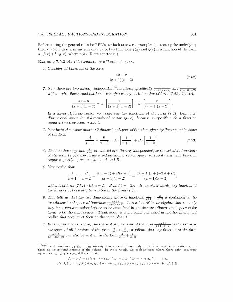
7.5. PARTIAL FRACTIONS AND INTEGRATION 651
Before stating the general rules for PFD’s, we look at several examples illustrating the underlyingtheory. (Note that a linear combination of two functions f(x) and g(x) is a function of the forma · f(x) + b · g(x), where a, b ∈ R are constants.)
Example 7.5.2 For this example, we will argue in steps.
1. Consider all functions of the form
ax + b
(x + 1)(x− 2). (7.52)
2. Now there are two linearly independent24functions, specifically x(x+1)(x−2) and 1
(x+1)(x−2)
which—with linear combinations—can give us any such function of form (7.52). Indeed,
ax + b
(x + 1)(x− 2)= a ·
[1
(x + 1)(x− 2)
]
+ b ·[
x
(x + 1)(x− 2)
]
.
In a linear-algebraic sense, we would say the functions of the form (7.52) form a 2-dimensional space (or 2-dimensional vector space), because to specify such a functionrequires two constants, a and b.
3. Now instead consider another 2-dimensional space of functions given by linear combinationsof the form
A
x + 1+
B
x− 2= A ·
[1
x + 1
]
+ B ·[
1
x− 2
]
. (7.53)
4. The functions 1x+1 and 1
x−2 are indeed also linearly independent, so the set of all functionsof the form (7.53) also forms a 2-dimensional vector space; to specify any such functionrequires specifying two constants, A and B.
5. Now notice that
A
x + 1+
B
x− 2=
A(x − 2) + B(x + 1)
(x + 1)(x− 2)=
(A + B)x + (−2A + B)
(x + 1)(x− 2),
which is of form (7.52) with a = A + B and b = −2A+ B. In other words, any function ofthe form (7.53) can also be written in the from (7.52).
6. This tells us that the two-dimensional space of functions Ax+1 + B
x−2 is contained in the
two-dimensional space of functions ax+b(x+1)(x−2) . It is a fact of linear algebra that the only
way for a two-dimensional space to be contained in another two-dimensional space is forthem to be the same spaces. (Think about a plane being contained in another plane, andrealize that they must then be the same plane.)
7. Finally, since (by 6 above) the space of all functions of the form ax+b(x+1)(x−2) is the same as
the space of all functions of the form Ax+1 + B
x−2 , it follows that any function of the formax+b
(x+1)(x−2) can also be written in the form Ax+1 + B
x−2 .
24We call functions f1, f2, · · · , fn linearly independent if and only if it is impossible to write any ofthese as linear combinations of the others. In other words, we exclude cases where there exist constants
a1, · · · , ak−1, ak+1, · · · , an ∈ R such that
fk = a1f1 + a2f2 + · · · + ak−1fk−1 + ak+1fk+1 + · · · + anfn, i.e.,
(∀x)[fk(x) = a1f1(x) + a2f2(x) + · · · + ak−1fk−1(x) + ak+1fk+1(x) + · · · + anfn(x)].
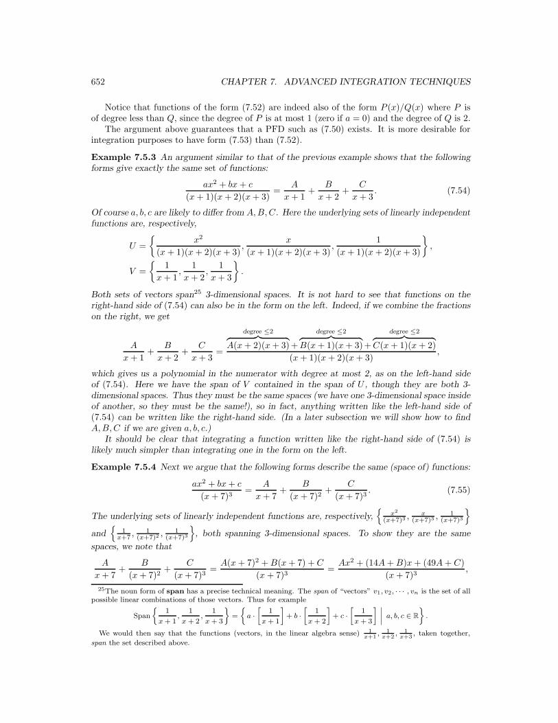
652 CHAPTER 7. ADVANCED INTEGRATION TECHNIQUES
Notice that functions of the form (7.52) are indeed also of the form P (x)/Q(x) where P isof degree less than Q, since the degree of P is at most 1 (zero if a = 0) and the degree of Q is 2.
The argument above guarantees that a PFD such as (7.50) exists. It is more desirable forintegration purposes to have form (7.53) than (7.52).
Example 7.5.3 An argument similar to that of the previous example shows that the followingforms give exactly the same set of functions:
ax2 + bx + c
(x + 1)(x + 2)(x + 3)=
A
x + 1+
B
x + 2+
C
x + 3. (7.54)
Of course a, b, c are likely to differ from A, B, C. Here the underlying sets of linearly independentfunctions are, respectively,
U =
{x2
(x + 1)(x + 2)(x + 3),
x
(x + 1)(x + 2)(x + 3),
1
(x + 1)(x + 2)(x + 3)
}
,
V =
{1
x + 1,
1
x + 2,
1
x + 3
}
.
Both sets of vectors span25 3-dimensional spaces. It is not hard to see that functions on theright-hand side of (7.54) can also be in the form on the left. Indeed, if we combine the fractionson the right, we get
A
x + 1+
B
x + 2+
C
x + 3=
degree ≤2︷ ︸︸ ︷
A(x + 2)(x + 3)+
degree ≤2︷ ︸︸ ︷
B(x + 1)(x + 3)+
degree ≤2︷ ︸︸ ︷
C(x + 1)(x + 2)
(x + 1)(x + 2)(x + 3),
which gives us a polynomial in the numerator with degree at most 2, as on the left-hand sideof (7.54). Here we have the span of V contained in the span of U , though they are both 3-dimensional spaces. Thus they must be the same spaces (we have one 3-dimensional space insideof another, so they must be the same!), so in fact, anything written like the left-hand side of(7.54) can be written like the right-hand side. (In a later subsection we will show how to findA, B, C if we are given a, b, c.)
It should be clear that integrating a function written like the right-hand side of (7.54) islikely much simpler than integrating one in the form on the left.
Example 7.5.4 Next we argue that the following forms describe the same (space of) functions:
ax2 + bx + c
(x + 7)3=
A
x + 7+
B
(x + 7)2+
C
(x + 7)3. (7.55)
The underlying sets of linearly independent functions are, respectively,{
x2
(x+7)3 , x(x+7)3 , 1
(x+7)3
}
and{
1x+7 , 1
(x+7)2 , 1(x+7)3
}
, both spanning 3-dimensional spaces. To show they are the same
spaces, we note that
A
x + 7+
B
(x + 7)2+
C
(x + 7)3=
A(x + 7)2 + B(x + 7) + C
(x + 7)3=
Ax2 + (14A + B)x + (49A + C)
(x + 7)3,
25The noun form of span has a precise technical meaning. The span of “vectors” v1, v2, · · · , vn is the set of allpossible linear combinations of those vectors. Thus for example
Span
1
x + 1,
1
x + 2,
1
x + 3
ff
=
a ·»
1
x + 1
–
+ b ·»
1
x + 2
–
+ c ·»
1
x + 3
– ˛
˛
˛
˛
a, b, c ∈ R
ff
.
We would then say that the functions (vectors, in the linear algebra sense) 1x+1
, 1x+2
, 1x+3
, taken together,
span the set described above.

7.5. PARTIAL FRACTIONS AND INTEGRATION 653
thus simplifying to the form on the left-hand side of (7.55), with a = A, b = 14A + B, andc = 49A + C, all constants. Arguing as before, the underlying sets of linearly independentfunctions must span the same 3-dimensional spaces, so anything of the form on the left-handside of (7.55) can be written also in the form on the right-hand side.
Example 7.5.5 For our last example, we claim the following forms give the same functions:
ax4 + bx3 + cx2 + dx + e
x3(x2 + 1)=
A
x+
B
x2+
C
x3+
Dx + E
x2 + 1. (7.56)
Here the spanning sets of linearly independent functions are respectively26
U =
{x4
x3(x2 + 1),
x3
x3(x2 + 1),
x2
x3(x2 + 1),
x
x3(x2 + 1),
1
x3(x2 + 1)
}
,
V =
{1
x,
1
x2,
1
x3,
x
x2 + 1,
1
x2 + 1
}
.
Again, the form on the right of (7.56) can be rewritten as below, simplifying into the formon the left-hand side of (7.56) as
Ax2(x2 + 1) + Bx(x2 + 1) + C(x2 + 1) + (Dx + E)(x2 + 1)
x3(x2 + 1)
=Ax4 + (B + D)x3 + (A + C + E)x2 + (B + D)x + (C + E)
x3(x2 + 1). (7.57)
(Note that this has numerator of degree at most 4.) So anything that is a linear combination offunctions of V can also be written as a linear combination of functions of U . Because both sidesof (7.56) must therefore describe exactly the same functions in a 5-dimensional vector space, itfollows that anything written in the form on the left-hand side of (7.56) can also be written inthe form on the right-hand side.
Note that it is a little tricky to find the new coefficients of 1, x, x2, x3, etc., in the newnumerator of (7.57). They all follow from gathering what we would get if we multiplied outthe original numerator, but it would be easy to miss a term. (The reader should verify thecomputation (7.57).)
In the next subsection we generalize the logic of the examples above to write exact rules forthe form of a PFD based upon the original fraction’s denominator. Then in Subsection 7.5.3we look at three methods of finding the coefficients, A, B, C, etc., of the PFD expansion, andimmediately apply the methods to problems of computing integrals of such functions.
26Of course we can also simplify the functions in U as the five linearly independent functions
U =
x
x2 + 1,
1
x2 + 1,
1
x(x2 + 1),
1
x2(x2 + 1),
1
x3(x2 + 1)
ff
.

654 CHAPTER 7. ADVANCED INTEGRATION TECHNIQUES
7.5.2 Partial Fraction Decompositions: The Rules
It is a fact of algebra (corollary to the Fundamental Theorem of Algebra) that any polynomialwith real coefficients can be factored uniquely—up to rearrangement of multiplicative constants—into powers of linear terms (ax+b)n and powers of irreducible quadratic27 terms (ax2 +bx+c)m
with real coefficients. So for instance,
x3 − x2 + x− 1 = (x− 1)(x2 + 1),
and there is no other way to factor it, except for instance 2(x− 1)(12x2 + 1
2 ), etc. With that inmind, the rules for partial fraction decompositions follow.
First, we are given a rational function P (x)Q(x) , where P and Q are polynomials.
0. In 1 and 2 below we assume deg P < deg Q. If the deg P ≥ deg Q, then first we applypolynomial long division to achieve
P (x)
Q(x)= p(x) +
r(x)
Q(x),
where p, r are polynomials and deg r < deg Q. Then the following rules apply to r(x)Q(x) .
1. If (ax+b)n, where a 6= 0 occurs as a factor in Q(x), then the partial fraction decomposition
(PFD) of P (x)Q(x) will contain terms
A1
ax + b+
A2
(ax + b)2+ · · ·+ An
(ax + b)n.
2. If ax2 + bx + c is an irreducible quadratic, and (ax2 + bx + c)m occurs as a factor in Q(x),
then the PFD of P (x)Q(x) will contain terms
A1x + B1
ax2 + bx + c+
A2x + B2
(ax2 + bx + c)2+ · · ·+ Amx + Bm
(ax2 + bx + c)m.
The application of these rules can be somewhat confusing at first, so we will look at severalexamples before proceeding to solve for the coefficients A1, B1, etc. For the second case, we willmostly be interested in irreducible quadratics of the form x2 + k2, where k > 0. Note that wewill usually use letters without subscripts, such as A, B, C, and so on for our PFD coefficients(to be found later).
Example 7.5.6 Write the partial fraction decompositions for the given rational functions:� 3x5 − 11x3 + 15x− 2
(x + 1)2(x− 3)4=
A
x + 1+
B
(x + 1)2+
C
x− 3+
D
(x− 3)2+
E
(x− 3)3+
F
(x− 3)4.� 1
(x + 1)2(x− 3)4=
A
x + 1+
B
(x + 1)2+
C
x− 3+
D
(x − 3)2+
E
(x− 3)3+
F
(x− 3)4.
27It is easy to see when a quadratic term is “irreducible over the real numbers,” meaning we cannot write itas (ex + f)(gx + h), where e, f, g, h ∈ R, the latter being equivalent to there being real numbers α, β such thatthe polynomial is zero there (i.e., at α = −f/e, β = −h/g). Using the quadratic formula, it is plain that no suchreal solutions to the quadratic being zero occur if and only if b2 − 4ac < 0 (i.e., when the term under the radicalin the quadratic formula is negative).
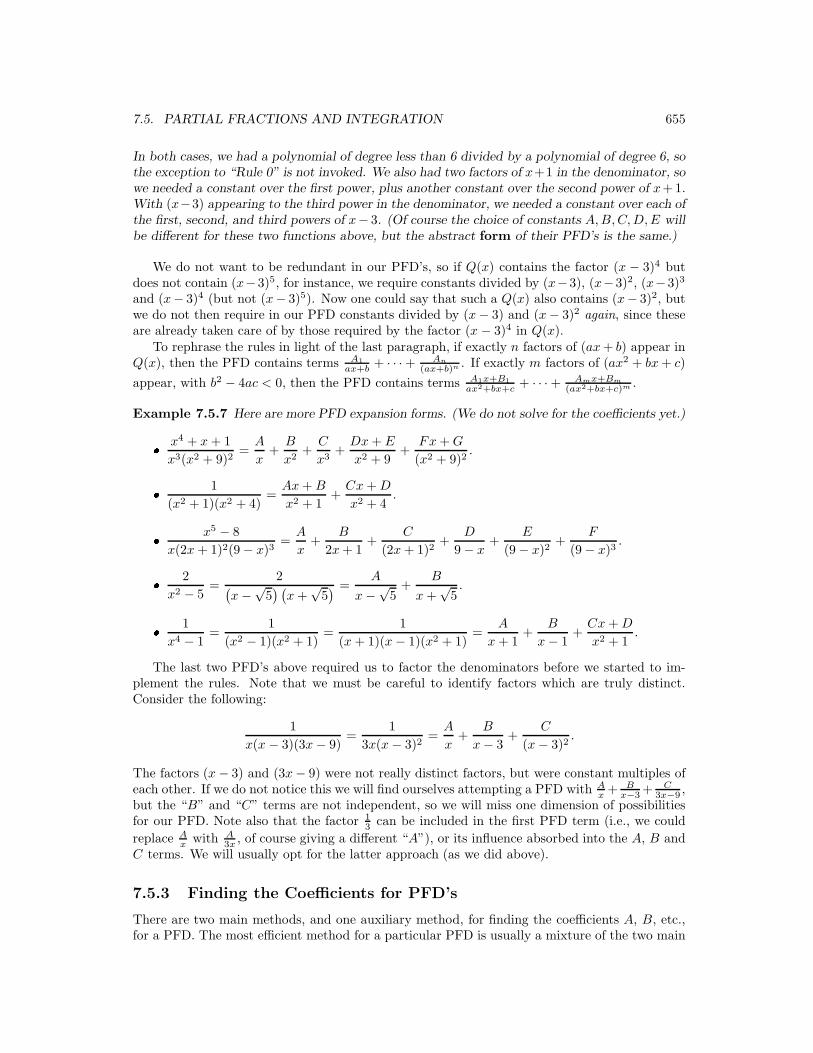
7.5. PARTIAL FRACTIONS AND INTEGRATION 655
In both cases, we had a polynomial of degree less than 6 divided by a polynomial of degree 6, sothe exception to “Rule 0” is not invoked. We also had two factors of x+1 in the denominator, sowe needed a constant over the first power, plus another constant over the second power of x+1.With (x−3) appearing to the third power in the denominator, we needed a constant over each ofthe first, second, and third powers of x− 3. (Of course the choice of constants A, B, C, D, E willbe different for these two functions above, but the abstract form of their PFD’s is the same.)
We do not want to be redundant in our PFD’s, so if Q(x) contains the factor (x − 3)4 butdoes not contain (x−3)5, for instance, we require constants divided by (x−3), (x−3)2, (x−3)3
and (x− 3)4 (but not (x− 3)5). Now one could say that such a Q(x) also contains (x− 3)2, butwe do not then require in our PFD constants divided by (x− 3) and (x− 3)2 again, since theseare already taken care of by those required by the factor (x − 3)4 in Q(x).
To rephrase the rules in light of the last paragraph, if exactly n factors of (ax + b) appear inQ(x), then the PFD contains terms A1
ax+b + · · ·+ An
(ax+b)n . If exactly m factors of (ax2 + bx + c)
appear, with b2 − 4ac < 0, then the PFD contains terms A1x+B1
ax2+bx+c + · · ·+ Amx+Bm
(ax2+bx+c)m .
Example 7.5.7 Here are more PFD expansion forms. (We do not solve for the coefficients yet.)� x4 + x + 1
x3(x2 + 9)2=
A
x+
B
x2+
C
x3+
Dx + E
x2 + 9+
Fx + G
(x2 + 9)2.� 1
(x2 + 1)(x2 + 4)=
Ax + B
x2 + 1+
Cx + D
x2 + 4.� x5 − 8
x(2x + 1)2(9− x)3=
A
x+
B
2x + 1+
C
(2x + 1)2+
D
9− x+
E
(9− x)2+
F
(9− x)3.� 2
x2 − 5=
2(x−√
5) (
x +√
5) =
A
x−√
5+
B
x +√
5.� 1
x4 − 1=
1
(x2 − 1)(x2 + 1)=
1
(x + 1)(x− 1)(x2 + 1)=
A
x + 1+
B
x− 1+
Cx + D
x2 + 1.
The last two PFD’s above required us to factor the denominators before we started to im-plement the rules. Note that we must be careful to identify factors which are truly distinct.Consider the following:
1
x(x − 3)(3x− 9)=
1
3x(x− 3)2=
A
x+
B
x− 3+
C
(x− 3)2.
The factors (x− 3) and (3x− 9) were not really distinct factors, but were constant multiples ofeach other. If we do not notice this we will find ourselves attempting a PFD with A
x + Bx−3 + C
3x−9 ,but the “B” and “C” terms are not independent, so we will miss one dimension of possibilitiesfor our PFD. Note also that the factor 1
3 can be included in the first PFD term (i.e., we could
replace Ax with A
3x , of course giving a different “A”), or its influence absorbed into the A, B andC terms. We will usually opt for the latter approach (as we did above).
7.5.3 Finding the Coefficients for PFD’s
There are two main methods, and one auxiliary method, for finding the coefficients A, B, etc.,for a PFD. The most efficient method for a particular PFD is usually a mixture of the two main
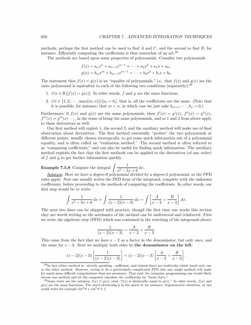
656 CHAPTER 7. ADVANCED INTEGRATION TECHNIQUES
methods; perhaps the first method can be used to find A and C, and the second to find B, forinstance. Efficiently computing the coefficients is thus somewhat of an art.28
The methods are based upon some properties of polynomials. Consider two polynomials
f(x) = anxn + an−1xn−1 + · · ·+ a2x
2 + a1x + a0,
g(x) = bmxm + bm−1xm−1 + · · ·+ b2x
2 + b1x + b0.
The statement that f(x) = g(x) is an “equality of polynomials,” i.e., that f(x) and g(x) are thesame polynomial is equivalent to each of the following two conditions (separately):29
1. (∀x ∈ R)[f(x) = g(x)]. In other words, f and g are the same functions.
2. (∀i ∈ {1, 2, · · · , max{m, n}})[ai = bi], that is, all the coefficients are the same. (Note thatit is possible, for instance, that m < n, in which case we just take bm+1, · · · , bn = 0.)
Furthermore, if f(x) and g(x) are the same polynomials, then f ′(x) = g′(x), f ′′(x) = g′′(x),f ′′′(x) = g′′′(x) · · · , in the sense of being the same polynomials, and so 1 and 2 from above applyto these derivatives as well.
Our first method will exploit 1, the second 2, and the auxiliary method will make use of finalobservation about derivatives. The first method essentially “probes” the two polynomials atdifferent points, usually chosen strategically, to get some quick information out of a polynomialequality, and is often called an “evaluation method.” The second method is often referred toas “comparing coefficients,” and can also be useful for finding quick information. The auxiliarymethod exploits the fact that the first methods can be applied to the derivatives (of any order)of f and g to get further information quickly.
Example 7.5.8 Compute the integral
∫1
x2 − 5x + 6dx.
Solution: Here we have a degree-0 polynomial divided by a degree-2 polynomial, so the PFDrules apply. Now one usually writes the PFD form of the integrand, complete with the unknowncoefficients, before proceeding to the methods of computing the coefficients. In other words, ourfirst step would be to write:
∫1
x2 − 5x + 6dx =
∫1
(x− 2)(x− 3)dx =
∫ [A
x− 2+
B
x− 3
]
dx.
The next two lines can be skipped with practice, though the first time one works this sectionthey are worth writing so the mechanics of the method can be understood and reinforced. Firstwe write the algebraic step (PFD) which was contained in the rewriting of the integrands above:
1
(x − 2)(x− 3)=
A
x− 2+
B
x− 3.
This came from the fact that we have x − 2 as a factor in the denominator, but only once, andthe same for x− 3. Next we multiply both sides by the denominator on the left:
(x− 2)(x− 3)
[1
(x− 2)(x− 3)
]
= (x− 2)(x− 3)
[A
x− 2+
B
x− 3
]
.
28In fact either method is—strictly speaking—sufficient, and indeed there are textbooks which teach only oneor the other method. However, trying to fit a particularly complicated PFD into any single method will makefor much more difficult computations than are necessary. That said, for computer programming one would likelychoose one method and let the computer calculate the coefficients by “brute force.”
29Some texts use the notation f(x) ≡ g(x), read “f(x) is identically equal to g(x).” In other words, f(x) andg(x) are the same functions. The word identically is in the spirit of, for instance, trigonometric identities, so onecould write for example sin2 θ + cos2 θ ≡ 1.

7.5. PARTIAL FRACTIONS AND INTEGRATION 657
On the left, the whole denominator cancels and we have the numerator of the original fraction.(This always happens.) On the right we have to distribute the (x− 2)(x− 3) across the sum inthe brackets. For the “A” term the (x − 2) cancels, while for the “B” term the (x− 3) cancels,giving us an equality of polynomials:
1 = A(x− 3) + B(x − 2). (7.58)
Because this is an equality of polynomials (f(x) = g(x) where f(x) = 1 and g(x) = A(x − 3) +B(x − 2)), it must be true for any x ∈ R. Now we choose two values of x strategically.
x = 3 : 1 = A(3− 3) + B(3 − 2) =⇒ 1 = B
x = 2 : 1 = A(2− 3) + B(2 − 2)
=⇒ 1 = −A =⇒ A = −1 .
Now we summarize what we have so far, and compute the desired integral:∫
1
x2 − 5x + 6dx =
∫ [ −1
x− 2+
1
x− 3
]
dx
= − ln |x− 2|+ ln |x− 3|+ C
= ln
∣∣∣∣
x− 3
x− 2
∣∣∣∣+ C.
(The last step is not necessary, but for reasons of style many textbooks combine logarithmicterms into a single logarithm.)
Because (7.58) was an equality of polynomials (meaning the polynomial on the left is the
same polynomial as that on the right30), we could substitute any number for x in (7.58) andstill have a true statement. Fortunately, there were choices which could eliminate an unknown,leaving an equation in the other unknown which is easily solved.
The second method for finding A and B (not preferred here but not terribly difficult hereeither) is to look at the coefficients of the polynomials on the left-hand side and right-hand sideof (7.58), and realize that the coefficients of the various powers of x must agree for these tobe the same polynomials. Though perhaps not necessary for this simple case, one sometimesexpands the right-hand side and collects like terms
1 = (A + B)x + (−3A− 2B).
From this or just reading from (7.58), we can in turn set equal the coefficients of the x1 terms andthe constant (some say x0) terms to get the following system of two equations in two unknowns:
{0 = A + B1 = −3A − 2B.
(7.59)
The first equation came from the fact that there is no x1-term on the left-hand side of (7.59),or alternatively, the x1-term is 0x1 on the left. To solve such a system one might add three
30It should be pointed out that when we write a PFD, for instance
1
(x − 2)(x − 3)=
A
x − 2+
B
x − 3,
we mean that these are the same functions as well, so once we find A and B, the right-hand side would simplifyto become the left-hand side. To find A and B we actually solve the polynomial equality (7.58) for A and B.
Note also the distinction between “equations” such as 2x−1 = 5, which is true only for x = 3, and “equalities”such as (x+1)2 = x2 +2x+1, true for all x, meaning the function (x+1)2 is the same as the function x2 +2x+1.

658 CHAPTER 7. ADVANCED INTEGRATION TECHNIQUES
times the first equation to the second, to get B = 1, and use that information in the first to getA = −1, as before.
Whenever the denominator of our function P (x)/Q(x) has a linear factor (ax+b), evaluatingthe associated polynomial equality—such as (7.58)—at that x-value which makes this linearfactor zero (namely x = −b/a) will quickly yield one of the coefficients, since all but one term inthe polynomial equation will have (ax + b) as a factor, and therefore vanish at x = −b/a. Thusthis first method should always be employed to find that coefficient if the denominator Q has alinear factor. If the denominator has all linear terms to the first power, then this “evaluation”method will quickly yield all coefficients.
Example 7.5.9 Compute
∫2x2 − 3x + 2
x(x + 5)(2x + 1)dx.
Solution: It is important to notice that the numerator is degree 2, and the denominatordegree 3, so the PFD rules do apply.
∫2x2 − 3x + 2
x(x + 5)(2x + 1)dx =
∫ [A
x+
B
x + 5+
C
2x + 1
]
dx.
Eventually we will cease writing the next two lines, but to be sure we will include them here sothat the logic is clear:
2x2 − 3x + 2
x(x + 5)(2x + 1)=
A
x+
B
x + 5+
C
2x + 1
=⇒ x(x + 5)(2x + 1)
[2x2 − 3x + 2
x(x + 5)(2x + 1)
]
= x(x + 5)(2x + 1)
[A
x+
B
x + 5+
C
2x + 1
]
=⇒ 2x2 − 3x + 2 = A(x + 5)(2x + 1) + Bx(2x + 1) + Cx(x + 5).
Into this last line we can now enter values for x which will quickly yield the coefficients.
x = 0 : 2 = A(5)(1) =⇒ A =2
5
x = −5 : 50 + 15 + 2 = B(−5)(−9)
=⇒ 67 = 45B =⇒ B =67
45.
x = −1
2: 2 · 1
4− 3 ·
(
−1
2
)
+ 2 = C
(
−1
2
) (
−1
2+ 5
)
=⇒ 1
2+
3
2+ 2 = C
(
−1
2
) (9
2
)
=⇒ 4 = −9
4C =⇒ C = −16
9.
Putting this together with our original integral, we get∫
2x2 − 3x + 2
x(x + 5)(2x + 1)dx =
∫ [2/5
x+
67/45
x + 5+−16/9
2x + 1
]
dx
=2
5ln |x|+ 67
45ln |x + 5| − 16
9· 12
ln |2x + 1|+ C
=2
5ln |x|+ 67
45ln |x + 5| − 8
9ln |2x + 1|+ C.
7.5. PARTIAL FRACTIONS AND INTEGRATION 659
Next we look at an example where all factors of Q(x) are linear, but one of these linear factorsappears to the second power.
Example 7.5.10 Compute
∫x + 1
x2(x − 5)(x + 4)dx.
Solution: This time we will describe but omit the explicit multiplication step in the PFD.31
∫x + 1
x2(x− 5)(x + 4)dx =
∫ [A
x+
B
x2+
C
x− 5+
D
x + 4
]
dx,
wherex + 1
x2(x− 5)(x + 4)=
A
x+
B
x2+
C
x− 5+
D
x + 4.
Multiplying by x2(x − 5)(x + 4) then gives us
x + 1 = Ax(x − 5)(x + 4) + B(x− 5)(x + 4) + Cx2(x + 4) + Dx2(x− 5). (7.60)
With this equation, choosing x = 0, 5,−4 will yield three of the four coefficients.
x = 0 : 1 = B(−5)(4) =⇒ B = − 1
20
x = 5 : 6 = C(52)(9)
=⇒ 2 · 352 · 3 · 3 = C =⇒ C =
2
75
x = −4 : −3 = D((−4)2)(−9)
=⇒ −3 = D[−16 · 9]
=⇒ 3 = D · 16 · 3 · 3 =⇒ D =1
48
This exhausts the evaluations which give equations in one coefficient. Next we have severalmethods for finding A.
Method 1. Compare coefficients. In particular, we look at the highest-order x-terms whichappear—at least initially—in the polynomial equality, which for (7.60) means the x3-terms. Here we have no x3-terms on the left, and on the right, even without a completeexpansion, we can see that the x3-terms will be A + C + D. (The middle-order terms aremore difficult to read from (7.60).) Fortunately we already know the values of C and D,so we have enough information to find A:
x3-term : 0 = A + C + D
=⇒ 0 = A +2
75+
1
48= A +
2
3 · 52+
1
24 · 3
⇐⇒ 0 = A +2 · 24 + 1 · 52
3 · 52 · 24= A +
32 + 25
3 · 52 · 24
⇐⇒ − 57
1200= A =⇒ A = − 19
400
31The pattern of cancellation, when we multiply the PFD by the original denominator Q(x), should becomesecond nature with a small amount of practice. That said, it is important to remember what we are doing(multiplying by Q(x)) to get from the PFD to the polynomial equality, and how the various factors cancel (or donot cancel) in that multiplication.
660 CHAPTER 7. ADVANCED INTEGRATION TECHNIQUES
From this we can complete the integration:
∫x + 1
x2(x− 5)(x + 4)dx =
∫ [− 19400
x+− 1
20
x2+
275
x− 5+
148
x + 4
]
dx
= − 19
400ln |x| − 1
20· −1
x+
2
75ln |x− 5|+ 1
48ln |x + 4|+ C.
Method 2. One can instead evaluate the polynomial equality (7.60) at still another x-value,though no such value will produce A alone:
x = 1 : 2 = A(1)(−4)(5) + B(−4)(5) + C(1)2(5) + D(1)2(−4).
Since we already know B, C and D, we can insert that information and solve for A.
Method 3. This will be more useful later, but this method (referred to earlier as the auxiliarymethod) certainly applies. The idea is that we apply d
dx to both sides of (7.60), which isvalid because the left-hand side and right-hand side of (7.60) are the same functions.
In order to use this method, it is useful to recall the generalized product rule. For threefunctions u(x), v(x) and w(x), for instance, we have
(uvw)′ = u′vw + uv′w + uvw′.
For reference we recall (7.60), from which we then compute the derivatives. Equation(7.60) reads:
x + 1 = Ax(x − 5)(x + 4) + B(x− 5)(x + 4) + Cx2(x + 4) + Dx2(x− 5).
d
dx: 1 = A[(1)(x − 5)(x + 4) + x(1)(x + 4) + x(x − 5)(1)]
+ B[(1)(x + 4) + (x− 5)(1)]
+ C[(2x)(x + 4) + x2(1)]
+ D[(2x)(x − 5) + x2(1)].
Now when we evaluate this at x = 0, we see that we get
1 = A[(1)(−5)(4)] + B[(1)(4) + (−5)(1)] + 0 + 0.
This gives us 1 = −20A−B, so then A = (1 + B)/(−20) = (19/20)/(−20) = −19/400, asbefore.
A simple principle buried in the third method is the following:
Theorem 7.5.1 If (x− a)m, where m > 1 is a factor of a polynomial f(x), then (x− a)m−1 is
a factor of f ′(x).
For a proof, we note that (x− a)m being a factor of f(x) is equivalent to f(x) = (x− a)mg(x),where g(x) is another polynomial. Thus
f ′(x) = (x− a)mg′(x) + m(x− a)m−1(1)g(x) = (x− a)m−1 [(x− a)g′(x) + mg(x)]︸ ︷︷ ︸
polynomial
,
7.5. PARTIAL FRACTIONS AND INTEGRATION 661
so indeed (x− a)m−1 is a factor of f ′(x).Now evaluating both sides of (7.60) at x = 0 caused those terms with x and x2 factors to
vanish, leaving an equation with B only. When we differentiate (7.60), those terms with x2
factors still vanish at x = 0—because one power of x remains—leaving only the B-term (asbefore) and the A-term (which had a factor x but not x2). Already knowing B, we could solvefor A.
A few guidelines for efficiently finding the PFD coefficients should be made at this point.
1. When linear factors are present in Q(x), it is best to exhaust this method for finding someof the coefficients easily. This means evaluating the relevant polynomial equality at eachvalue for which Q(x) = 0.
2. When those values are exhausted, we should next compare coefficients of the powers of x,particularly the highest power which occurs on the right-hand side.
3. If (ax + b)m is a factor of Q(x), where m > 1, and the first two methods fail to get allcoefficients, then differentiation of the polynomial equality may yield more coefficients.
4. If there are still coefficients to be found, then further evaluations, differentiations, or coef-ficient comparisons should be implemented.
Example 7.5.11 Compute
∫5x3 − 17x2 + 19x− 13
(x + 1)(x− 2)3dx.
Solution: As usual we start with the PFD, since the denominator has higher degree than thenumerator.
5x3 − 17x2 + 19x− 13
(x + 1)(x− 2)3=
A
x + 1+
B
x− 2+
C
(x− 2)2+
D
(x− 2)3
5x3 − 17x2 + 19x− 13 = A(x − 2)3 + B(x + 1)(x− 2)2 + C(x + 1)(x− 2) + D(x + 1) (7.61)
x = −1 : −5− 17− 19− 13 = A(−27)
=⇒ −54 = −27A =⇒ A = 2
x = 2 : 5(8)− 17(4) + 19(2)− 13 = D(3)
=⇒ −3 = 3D =⇒ D = −1
x3-term : 5 = A + B
=⇒ 5 = 2 + B =⇒ B = 3 .
While we could perform another evaluation (x = 0 comes to mind), or look at another coefficient(prone to error), instead we will differentiate (7.61):
15x2 − 34x + 19 = A[3(x− 2)2(1)]
+ B[(1)(x− 2)2 + (x + 1) · 2(x− 2)(1)]
+ C[(1)(x − 2) + (x + 1)(1)]
+ D(1).
Now we evaluated at x = 2:
15(4)− 34(2) + 19 = C(3) + D
=⇒ 11 = 3C − 1 =⇒ C = 4 .

662 CHAPTER 7. ADVANCED INTEGRATION TECHNIQUES
Thus∫
5x3 − 17x2 + 19x− 13
(x + 1)(x− 2)3dx =
∫ [2
x + 1+
3
x− 2+
4
(x− 2)2− 1
(x− 2)3
]
dx
= 2 ln |x + 1|+ 3 ln |x− 2| − 4
x− 2− 1
−2· 1
(x− 2)2+ C
= ln∣∣(x + 1)2(x− 2)3
∣∣− 4
x− 2+
1
2(x− 2)2+ C.
A quick corollary to our Theorem 7.5.1 is that if (x − a)m is a factor of a polynomial f(x),
then for k < m we have (x− a)m−k is a factor of f (k)(x) = dk
dxk f(x). This follows from repeatedapplications of the theorem, which can be paraphrased as saying that we lose at most one factorof (x−a) for each derivative we take, until we run out of factors of (x−a). If our latest examplehad (x− 2)4 in the denominator, we could have taken a second derivative of the correspondingpolynomial equation, and then those terms with (x − 2)3 or (x − 2)4 will still be zero at x = 2,but the other terms would likely be nonzero.32
Now we turn our attention to PFD’s where the denominators contain irreducible quadraticfactors.33 One problem with such factors is that they are nonzero for any x ∈ R,34 so theevaluation method’s usefulness is limited in these cases. For such PFD’s, we will need to relymore upon the coefficient comparison method to find our coefficients.
Example 7.5.12 Compute
∫4x3 − 7x2 + 31x− 38
x4 + 13x2 + 36dx.
Solution: PFD rules apply since the degree of the numerator is less than that of the denom-inator. We need to begin by factoring the denominator of the integrand, after which we canwrite the general form of the PFD.
∫4x3 − 7x2 + 31x− 38
x4 + 13x2 + 36dx =
∫4x3 − 7x2 + 31x− 38
(x2 + 4)(x2 + 9)dx =
∫ [Ax + B
x2 + 4+
Cx + D
x2 + 9
]
dx.
Now taking the second equation, we underlying PFD becomes the polynomial equality
4x3 − 7x2 + 31x− 38 = (Ax + B)(x2 + 9) + (Cx + D)(x2 + 4). (7.62)
Now we look at the coefficients.35
x3-term : 4 = A + C
x2-term : −7 = B + D
x1-term : 31 = 9A + 4C
x0-term : −38 = 9B + 4D.
32Note that it is quite possible that x− a is not a factor of a polynomial f(x), but is a factor of f ′(x). That isthe case when x = a is a critical point of f(x). For example, x − 1 is not a factor of f(x) = x2 − 2x + 21, but isa factor of f ′(x) = 2x − 2 = 2(x − 1).
Note also that the theorem applies to any linear factor ax + b, where a 6= 0, since ax + b = a“
x + b
a
”
. Thus
if xm is a factor of a polynomial f(x), the xm−1 is a factor of f ′(x), etc., as is the case if we replace xm with
(ax + b)m = am
“
x + b
a
”
.33Until the next section, we will not be able to integrate the general case where we have an irreducible quadratic
factor to a power greater than 1, with some exceptional cases.34Recall that if f(x) is a polynomial of degree ≥ 1, then f(a) = 0 ⇐⇒ (x − a) is a factor of f(x).35Note that the constant (“x0”) term equation is what we would get if we evaluated (7.62) at x = 0. It is easy
to see that this is always the case.
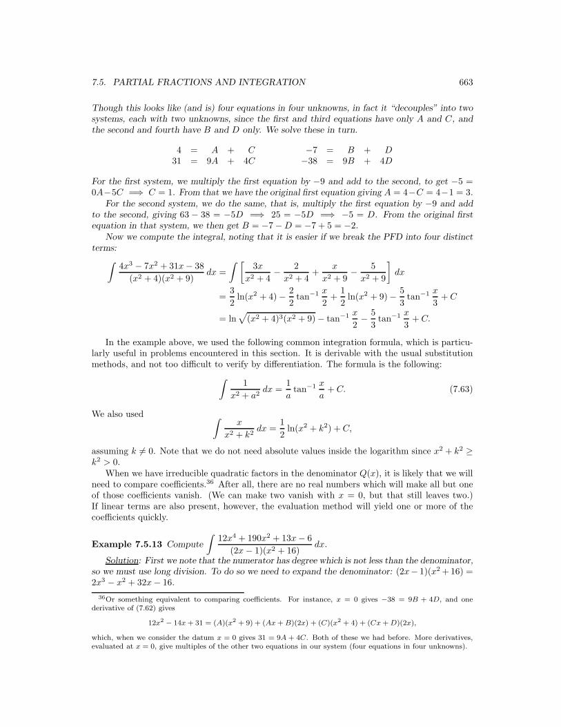
7.5. PARTIAL FRACTIONS AND INTEGRATION 663
Though this looks like (and is) four equations in four unknowns, in fact it “decouples” into twosystems, each with two unknowns, since the first and third equations have only A and C, andthe second and fourth have B and D only. We solve these in turn.
4 = A + C31 = 9A + 4C
−7 = B + D−38 = 9B + 4D
For the first system, we multiply the first equation by −9 and add to the second, to get −5 =0A−5C =⇒ C = 1. From that we have the original first equation giving A = 4−C = 4−1 = 3.
For the second system, we do the same, that is, multiply the first equation by −9 and addto the second, giving 63 − 38 = −5D =⇒ 25 = −5D =⇒ −5 = D. From the original firstequation in that system, we then get B = −7−D = −7 + 5 = −2.
Now we compute the integral, noting that it is easier if we break the PFD into four distinctterms:
∫4x3 − 7x2 + 31x− 38
(x2 + 4)(x2 + 9)dx =
∫ [3x
x2 + 4− 2
x2 + 4+
x
x2 + 9− 5
x2 + 9
]
dx
=3
2ln(x2 + 4)− 2
2tan−1 x
2+
1
2ln(x2 + 9)− 5
3tan−1 x
3+ C
= ln√
(x2 + 4)3(x2 + 9)− tan−1 x
2− 5
3tan−1 x
3+ C.
In the example above, we used the following common integration formula, which is particu-larly useful in problems encountered in this section. It is derivable with the usual substitutionmethods, and not too difficult to verify by differentiation. The formula is the following:
∫1
x2 + a2dx =
1
atan−1 x
a+ C. (7.63)
We also used ∫x
x2 + k2dx =
1
2ln(x2 + k2) + C,
assuming k 6= 0. Note that we do not need absolute values inside the logarithm since x2 + k2 ≥k2 > 0.
When we have irreducible quadratic factors in the denominator Q(x), it is likely that we willneed to compare coefficients.36 After all, there are no real numbers which will make all but oneof those coefficients vanish. (We can make two vanish with x = 0, but that still leaves two.)If linear terms are also present, however, the evaluation method will yield one or more of thecoefficients quickly.
Example 7.5.13 Compute
∫12x4 + 190x2 + 13x− 6
(2x− 1)(x2 + 16)dx.
Solution: First we note that the numerator has degree which is not less than the denominator,so we must use long division. To do so we need to expand the denominator: (2x− 1)(x2 + 16) =2x3 − x2 + 32x− 16.
36Or something equivalent to comparing coefficients. For instance, x = 0 gives −38 = 9B + 4D, and onederivative of (7.62) gives
12x2 − 14x + 31 = (A)(x2 + 9) + (Ax + B)(2x) + (C)(x2 + 4) + (Cx + D)(2x),
which, when we consider the datum x = 0 gives 31 = 9A + 4C. Both of these we had before. More derivatives,evaluated at x = 0, give multiples of the other two equations in our system (four equations in four unknowns).
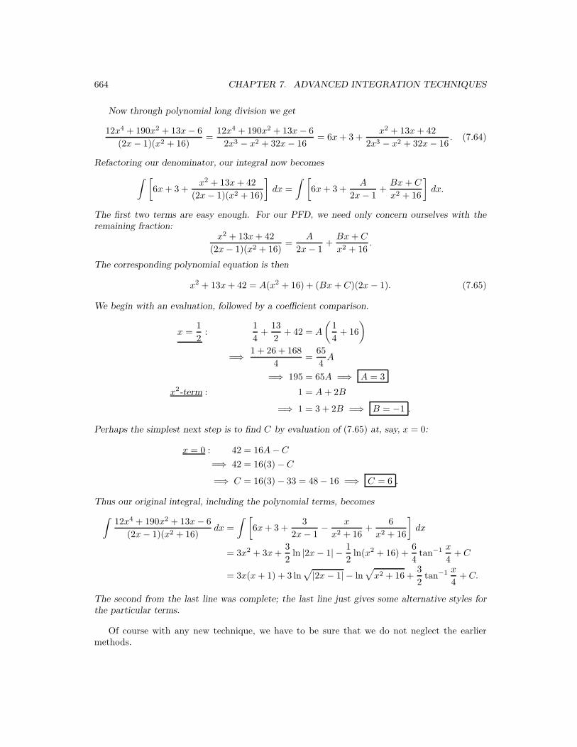
664 CHAPTER 7. ADVANCED INTEGRATION TECHNIQUES
Now through polynomial long division we get
12x4 + 190x2 + 13x− 6
(2x− 1)(x2 + 16)=
12x4 + 190x2 + 13x− 6
2x3 − x2 + 32x− 16= 6x + 3 +
x2 + 13x + 42
2x3 − x2 + 32x− 16. (7.64)
Refactoring our denominator, our integral now becomes
∫ [
6x + 3 +x2 + 13x + 42
(2x− 1)(x2 + 16)
]
dx =
∫ [
6x + 3 +A
2x− 1+
Bx + C
x2 + 16
]
dx.
The first two terms are easy enough. For our PFD, we need only concern ourselves with theremaining fraction:
x2 + 13x + 42
(2x− 1)(x2 + 16)=
A
2x− 1+
Bx + C
x2 + 16.
The corresponding polynomial equation is then
x2 + 13x + 42 = A(x2 + 16) + (Bx + C)(2x− 1). (7.65)
We begin with an evaluation, followed by a coefficient comparison.
x =1
2:
1
4+
13
2+ 42 = A
(1
4+ 16
)
=⇒ 1 + 26 + 168
4=
65
4A
=⇒ 195 = 65A =⇒ A = 3
x2-term : 1 = A + 2B
=⇒ 1 = 3 + 2B =⇒ B = −1 .
Perhaps the simplest next step is to find C by evaluation of (7.65) at, say, x = 0:
x = 0 : 42 = 16A− C
=⇒ 42 = 16(3)− C
=⇒ C = 16(3)− 33 = 48− 16 =⇒ C = 6 .
Thus our original integral, including the polynomial terms, becomes
∫12x4 + 190x2 + 13x− 6
(2x− 1)(x2 + 16)dx =
∫ [
6x + 3 +3
2x− 1− x
x2 + 16+
6
x2 + 16
]
dx
= 3x2 + 3x +3
2ln |2x− 1| − 1
2ln(x2 + 16) +
6
4tan−1 x
4+ C
= 3x(x + 1) + 3 ln√
|2x− 1| − ln√
x2 + 16 +3
2tan−1 x
4+ C.
The second from the last line was complete; the last line just gives some alternative styles forthe particular terms.
Of course with any new technique, we have to be sure that we do not neglect the earliermethods.

7.5. PARTIAL FRACTIONS AND INTEGRATION 665

666 CHAPTER 7. ADVANCED INTEGRATION TECHNIQUES
7.6 Miscellaneous Methods
In this section we will use completing the square, and other methods to rewrite several types ofintegrals into forms where we can more easily use either partial fractions or trigonometric substi-tution. We will also look at examples where a substitution will bring us to such forms. Finally,we will consider the use of integration tables, which can be found in numerous publications, butwhich require some sophistication to be used properly.