Advanced Industrial Organization I

Lecture 3: Demand & Market Structure

Måns Söderbom�

27 January 2009

�Department of Economics, University of Gothenburg. O¢ ce: E526. E-mail: mans.soderbom@economics.gu.se

1. Introduction

[Note: These notes contain the material I presented in lecture 3 - I�ve just used a di¤erent format in

order to conserve paper and facilitate printing. I have also corrected some typos].

References for this lecture:

� These notes.

� Chapters 2-3 in Pepall et al. (2008)

� Epple, Dennis and Bennett T. McCallum (2005). "Simultaneous Equation Econometrics: The

Missing Example".

� Ashenfelter, Orley, David Ashmore, Jonathan B. Baker, Suzanne Bleason and Daniel S. Hosken

(2005). "Econometric Methods in Staples," mimeo, Princeton University.

The papers by Epple & McCallum, and Ashenfelter et al. can be obtained from the course web-page.

� In the �rst part of this lecture I will discuss basic microeconomic theory of supply and demand,

and important issues that arise in empirical analysis of supply and demand.

� I begin by reviewing familiar models of �rm behaviour, looking at the case of perfect compe-

tition and monopoly, and show how optimal supply is determined in such models.

�By assuming that the market is in equilibrium, so that demand equals supply, I write down a

simple system of equations modelling supply and demand. These equations, no doubt, will be

very familiar to you.

� I then discuss important issues that arise when we want to estimate the parameters in the

supply-demand model. I begin by discussing what types of data will be needed. I then discuss

identi�cation. Finally, I link these points to choice of estimator.

�We will follow up on some of these points in the �rst group assignment, where we will use data

on chicken consumption & production in the U.S. for 1960-1999 to attempt to estimate supply

1

and demand functions. These data, which were used in the paper by Epple and McCallum

(2005).

� In the second part of the lecture I will discuss market structure and market power.

� In particular, I will focus on empirical methods that can be used for describing the maket structure,

and analyzing the consequences of di¤erent forms of market structure on �rm behaviour and,

ultimately, consumer welfare.

2. Perfect Competition & Monopoly: Market Outcomes

References:

� Ch. 2 in Pepall et al.

� Epple and McCallum (2005).

� Theories of perfect competition and monopoly were developed early in the literature and remain

central in industrial organization. In this section we review simple models for these types of market

structure, and investigate what the implications are for producer decisions.

� We assume that �rms seek to maximize pro�ts, and make their production decisions accordingly.

� As you know, the demand for the �rm�s product is a fundamental factor determining the production

decisions of the �rm.

� We take as given the derivation of an aggregate consumer demand curve. That is, we happily assume

that quantity demanded is a decreasing function of the price, and don�t worry about the details

involved in actually deriving this demand curve from consumers�utility maximization problem.

� The two most common functional forms for demand are

�Linear demand function, e.g.

QD = a� b� P;

2

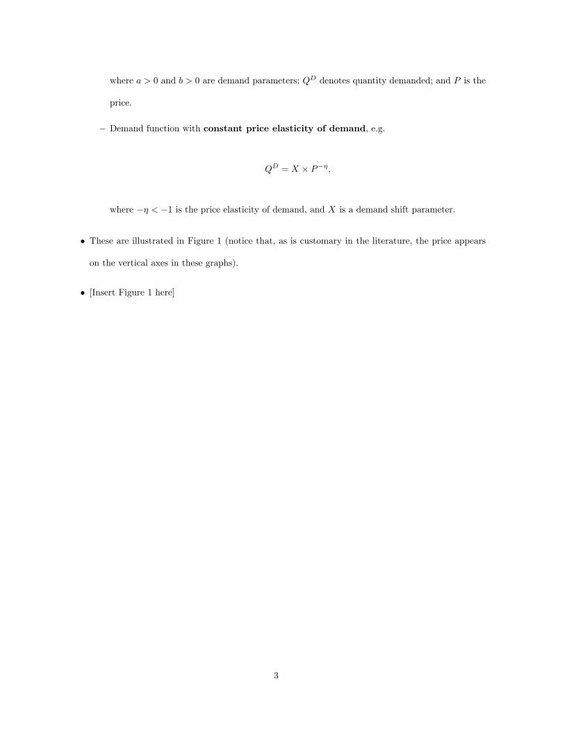
where a > 0 and b > 0 are demand parameters; QD denotes quantity demanded; and P is the

price.

�Demand function with constant price elasticity of demand, e.g.

QD = X � P��;

where �� < �1 is the price elasticity of demand, and X is a demand shift parameter.

� These are illustrated in Figure 1 (notice that, as is customary in the literature, the price appears

on the vertical axes in these graphs).

� [Insert Figure 1 here]

3

Figure 1: Two common demand functions

A. Demand Function: Constant Price Elasticity of Demand Quantity Demanded = 100,000*Price-3

B. Demand Function: Linear Quantity Demanded = 200 – 10*Price

1012

1416

1820

Pric

e

20 40 60 80 100Quantity

1012

1416

1820

Pric

e

0 20 40 60 80 100Quantity

Figure 2: Profits and quantity supplied for a single firm in a competitive market

-100

-80

-60

-40

-20

0P

rofit

0 5 10 15 20Quantity supplied by single firm

Note: P = 30, and C(q) = 100 + q2 + 10q. Profit = P*q – C(q). This example links to Practice Problem 2.1 in Pepall et al. (p. 25).

� Of course we can easily re-arrange the demand curves above, so as to put the price on the left-hand

side. This is known as the inverse demand function. For our two demand models:

� Linear inverse demand function:

P = A�B �QD;

where A = a=b;B = 1=b:(What�s the interpretation of A?)

� Inverse demand function with constant price elasticity of demand:

P = X1� �

�QD

�� 1� ;

� We need to be clear on the concept of equilibrium. The following will do as a de�nition: In

equilibrium, no consumer and no �rm has an incentive to change its decision on how much to buy

or produce. Nothing changes - the market is at rest.

� We will now look at market outcomes under perfect competition and monopoly.

2.1. Perfect competition

� We distinguish between short-run (SR) and long-run (LR) outcomes.

� In the short run, �xed capital (plant & equipment) is �xed - neither the number of �rms nor

the �xed capital at each �rm can be changed in response to changing market conditions.

� In the long run, in contrast, �xed capital can change.

� De�nition of perfect competition: Each �rm is a price taker - no individual �rm can in�uence

the market price. The price is determined by the interaction of all the �rms and consumers in the

market - more precisely, by aggregate supply and aggregate demand. Assumes that each �rm�s

potential supply of the product is "small" relative to total demand.

� The �rm perceives that it can sell as much, or as little, as it wants at the going price.

4

� Implication: Firm�s demand curve is �at.

� How can �rm�s demand curve be �at while the industry demand curve is downward sloping? This

follows from the de�nition above: under perfect competition, no individual �rm can a¤ect the price

by varying its output level. Hence, by de�nition, the price is invariant to changes in output made

by a single �rm. The industry demand curve, however, is determined by consumer preferences -

loosely speaking consumer preferences are such that the buyer will demand less of the good if the

price increases.

� [Draw the �rm�s demand curve, the industry demand curve, the industry supply curve]

� Single �rm�s decision: choose its output volume q so as to maximize pro�ts, given market price P :

maxqPq � C (q) ;

where C (q) includes costs of intermediate inputs (e.g. raw materials), labour, and the rate of return

on capital (so zero pro�ts - an implication under perfect competition as we shall see - doesn�t imply

that owners get nothing; they get the "normal" rate of return on capital). Note that P is not a

function of q here - re�ecting price taking behaviour, of course.

� Assuming the �rm�s pro�t is concave in q, we have the following �rst-order condition, necessary

and su¢ cient for pro�t maximization:

P � @C (q)@q

= 0

P =@C (q)

@q;

� Example (draws on Practice Problem 2.1 in Pepall et al): Suppose P = 30 and

C (q) = 100 + q2 + 10q

5

Figure 2 then shows how the �rm�s pro�t, de�ned

� = Pq � C (q) ;

varies with the quantity it supplies. Clearly maximum pro�ts is achieved at q = 10. We can easily

con�rm that this is consistent with the �rst-order condition above:

P =@C (q)

@q

P = 2q + 10

q =P � 102

;

and recall P = 30:

� [Figure 2 here]

6

� We have just derived the optimal supply of an individual �rm, given the prevailing price P . But

how is this price set in the �rst place? It�s important to remember that the equilibrium price in the

market is determined by industry supply and industry demand. It is also important to distinguish

between the short run and the long run. Let�s take these points in turn.

� Industry supply is simply total supply by all �rms in the market. If, as in the example above,

individual supply is

q =P � 102

;

and if there 50 �rms in the market, then industry supply is given by

QS =50P � 500

2= 25P � 250:

� Suppose industry demand is as follows:

QD =6000� 50P

9:

� In market equilibrium, we have QS = QD; hence P = 30 (con�rm this) is the equilbrium price.

� Each �rm will receive pro�ts as follows:

� = Pq � C (q)

� = 30� 10��100 + 102 + 10� 10

�� = 0;

i.e. there will be zero pro�ts in this particular equilibrium.

� In the long run equilibrium all �rms will make zero pro�ts. Otherwise it will not be an equilbrium

- if �rms are making pro�ts (over and above the natural return on capital), then more �rms will

7

enter the market and thus shift the aggregate supply function. Entry into the market will cease

exactly when all �rms are making zero pro�ts - hence this is the long run equilibrium.

� Notice that in the LR: total costs = total revenue (since zero pro�ts); hence average costs = price

= marginal cost.

� However, in the short run �rms in a competitive market can make pro�ts, since new �rms can�t

enter the market immediately (by assumption).

� To illustrate this point, suppose we start from the long run equilibrium derived above. Now suppose

there is a positive demand shock, so that the demand function shifts outward, from

QD =6000� 50P

9;

to

QD =8750� 50P

9:

How will this a¤ect the 50 existing �rms? We know that the supply of each individual �rm is

q =P � 102

;

and so, with 50 �rms in the market, the industry supply function is unchanged:

QS = 25P � 250:

The new (short-run) equilibrium implies

QD = QS

8750� 50P9

= 25P � 250

P = 40:

8

Hence the market equilibrium price has increased from 30 to 40. Each individual �rm now supplies

q =P � 102

= 15;

and so each individual �rm receives positive pro�ts:

� = Pq � C (q)

� = 40� 15��100 + 152 + 10� 15

�� = 125:

The reason this is a short-run, but not long-run, equilibrium, is that these pro�ts will trigger

entry of new �rms. This will shift the industry supply curve out, until entry stops as there are no

supernatural pro�ts to be made in the market.

2.2. Monopoly

� Now suppose all the sellers in the market become consolidated into one �rm - a monopoly.

� The monopoly�s demand curve is the industry�s demand curve.

� Hence the monopoly is able to in�uence the price.

� Monopolist�s decision: choose output volume q so as to maximize pro�ts, but take into account the

e¤ect of q on P :

maxqP (q) q � C (q) ;

where P (q) is the inverse demand curve.

9

� First-order condition:

@P (q)

@qq + P (q)� @C (q)

@q= 0�

@P (q)

@q

q

P (q)+ 1

�P (q) =

@C (q)

@q��1�+ 1

�P (q) =

@C (q)

@q;

where � > 1 is the elasticity of demand, measuring how responsive the quantity demanded is to

price movements.

� One interpretation of this is that the �rm chooses q so as to result in an output price that exceeds

the marginal cost:

P (q) =@C (q)

@q

��1�+ 1

��1=

@C (q)

@q

��

� � 1

�>@C (q)

@q

The steeper the slope of the demand curve, the less elastic is demand, and so the higher is the

markup.

� The monopolist makes a pro�t over and above the normal return on capital

� Because the monopolist is the only �rm in this market, and because we assume no other �rm can

enter the market, this is a long-run equilibrium - i.e. even in the long run there is no tendency for

the market price to equal the unit cost of production.

This concludes my brief overview of the perfect competition and monopoly.

� I will not discuss the material in Pepall et al. (2008) on present discounted value (Section 2.2)

because I assume you know it already. Please read this section on your own.

� I will also skip Sections 2.3-4 in the book, which contain a discussion of e¢ ciency. Please read on

your own.

10

3. Empirical Analysis of Demand and Supply: Setting the Scene

Reference: Epple and McCallum (2005).

In this section we consider a simple supply-demand model, in which the market price P and the

quantity q are jointly determined by demand and supply, and discuss how we can use data to estimate

parameters of interest. Homogeneous good.

� We continue to take demand as a given - i.e. we don�t derive explicitly it from consumer preferences

(but, of course, we understand that demand is determined by preferences and income). Suppose we

write demand in period t in constant elasticity form:

qt = XtP��t ;

where �� < �1 is the price elasticity of demand, and Xt is a demand shift parameter. Thus high

values of Xt (could be income - see paper) will be associated with high demand, and vice versa; i.e.

changes in Xt will shift the demand curve, and thus in�uence the equilibrium price.

� To motivate the supply curve, consider the �rst-order condition for the monopolist:

��1�+ 1

�P (q) =

@C (q)

@q;

which says that the monopolist will supply the quantity q for which the marginal revenue is equal

to the marginal cost. This means we can identify two categories of driving factors of supply:

�The demand: Think of P (q) as the inverse demand curve, hence shocks to demand will

in�uence equilibrium price.

�The �rm�s technology: Recall that C (q) represents the �rm�s total cost of producing q. Now

modify the cost function so that the production cost explicitly depends on input prices W :

C = C (q;W ) ;

11

Given that the cost function is a monotonically increasing function of output produced (seems

very reasonable), we can invert the cost function and write quantity supplied as

qt = S (Pt;Wt) :

� Supply in logarithmic form:

qst = �0 + �1pt + �2wt + ut (3.1)

� Demand in logarithmic form:

qdt = �0 + �1pt + �2yt + vt (3.2)

� Parameters: �1 > 0; �2 < 0; �1 < 0;�2 > 0.

� Equations (3.1) and (3.2) form a system of equations in structural form, in the sense that each

equation speci�es causal, theoretical relationships. The parameter �1 is interpretable as the price

elasticity of demand, for example - a key parameter in our theoretical model.

� Suppose our goal is to estimate the parameters of the model. What type of data do we need?

�Quantity supplied & demanded

�Output price

�Demand shifters - e.g. income y

� Supply shifters - e.g. input prices w

� Our empirical equations:

qst = �0 + �1pt + �2wt + ut (Supply)

qdt = �0 + �1pt + �2yt + vt (Demand)

� Equilibrium:

qst = qdt

12

� Econometrics: Price is an endogenous variable. To see this, combine the supply and demand

equations and solve for price and quantity in reduced form. You will obtain equations of the

following form:

q = �1wt + �2yt + �1 (ut; vt)

p = !1wt + !2yt + �2 (ut; vt) :

Clearly a shock to demand (vt) will impact on the price - hence price is endogenous.

� Identi�cation: Suppose our goal is to estimate the parameter �1, which measures the causal e¤ect

of a change in the price on quantity demanded. That is, this parameter measures the slope of the

demand function.

� In the language of simultaneous equation econometrics, we cannot identify �1 unless the rank and

order conditions are ful�lled (see an econometrics book if you are interested).

� More intuitively, we cannot infer �1 from the observed relationship in the data between quantity

and price, because we can�t be sure about whether this relationship in the data re�ects movement

along the demand curve, the supply curve, or a combination.

� [Illustration of identi�cation problem]

� To identify the demand curve, we need to come up with a way of holding demand constant while

varying supply.

� Instrumental variables: instrument the price variable using supply side variables - in the model

above, this means we need

� �2 6= 0, or otherwise we cannot identify �1. Intuitively, the reason is that, while q depends on

p, causation runs in the opposite direction as well. By using an IV approach, we consider how

movements in the price that are only attributable to supply side shocks correlate with quantities

13

produced and consumed. Our theory then tells us we can interpret the results as telling us what

the demand curve looks like.

4. Causality in Applied Econometrics

� Goal of most empirical studies in economics: investigate if and how a change in an �explanatory�

variable X causes a change in another variable Y , the dependent variable - in our context, how a

change in the price causes demand to fall.

� In order to �nd the causal e¤ect, we must hold all other relevant determinants of Y �xed - ceteris

paribus analysis. In the social sciences, we rarely have access to data generated in a laboratory

(where the analyst controls the explanatory variables). We therefore need a technique that enables

us to analyze the data and draw inferences about the role played byX as if other factors determining

y are held �xed.

� Regression analysis is one such approach.

� Wemay achieve a lot by including control variables in our regressions. But when estimating demand-

supply models, you typically suspect you don�t observe all relevant determinants of demand and

supply. As a result, the theory tells us we will have an endogeneity problem.

4.0.1. Instrumental Variables

Arguably the most important econometric problem for estimation of the demand-supply model is posed

by the output price being likely endogenous. Suppose my goal is to estimate the price elasticity of

demand. To do this, I consider the demand equation

qt = �0 + �1pt + �2yt + vt:

My problem is that the output price pt is determined jointly with quantity demanded. In particular,

a shock to demand not captured by income y (like what?) is likely to a¤ect the price. Where in our

14

demand equation above would such a shock enter?

It would enter the residual vt. If, as a result, the residual vt is correlated with the price, we clearly

have an endogeneity problem.

Some of you may be very familiar with the instrumental variables approach, others may not. In this

subsection, I brie�y discuss the following:

� The key assumptions that need to hold for the IV approach to work

� How the IV estimator works

� Some intuition into why it works

My exposition is informal but hopefully su¢ cient given our current purposes. If you have di¢ culties,

you need to consult a basic econometrics textbook (I�d recommend "Introductory Econometrics" by

Je¤rey Wooldridge, or "A Guide to Modern Econometrics" by Marco Verbeek, but there are many others

too).

4.0.2. Two key assumptions underlying the IV approach

� We suspect that the residual in our demand equation is correlated with the market price:

qt = �0 + �1pt + �2yt + vt:

cov (pt; vt) 6= 0.

This amounts to saying that the price is econometrically endogenous.

� Now, the price varies for many reasons. In our model, the price varies because of shocks to supply

and shocks to demand:

pt = �1 � wt + �2 � yt + et;

where �1; �2 are non-zero coe¢ cients. Price will clearly be correlated with a determinant of supply

in this case (i.e. the input price variable wt). The key point, however, is that if wt is uncorrelated

15

with shocks to demand, then there is some variation in the price that is not correlated with

demand shocks. That is, there is some exogenous variation in the price.

� The IV estimator uses only this source of variation in the price to identify the demand curve. Note

the analogy with moving around the supply curve whilst holding demand constant.

� We say that wt is our instrument (by which we really mean there is an exclusion restriction: wt

does not enter the structural demand equation - it is excluded).

� For the IV estimator to work, the following conditions need to hold:

cov (wt; vt) = 0; (4.1)

cov (wt; pt) 6= 0: (4.2)

� The �rst of the conditions, (4.1), says that the instrument must be uncorrelated with the residual

in the demand equation. This is sometimes referred to as instrument validity.

� The second condition, (4.2), says that the instrument must be correlated with the endogenous

explanatory variable, i.e the price This is sometimes referred to as instrument relevance.

� If these conditions hold, then wt can be used as an instrument for the price in the demand equation.

4.0.3. How the IV estimator works

� We can obtain an instrumental variable estimate by means of a two-stage procedure:

1. Run an OLS regression in which price is the dependent variable, and the instrument wt; and other

exogenous variables in the model are the explanatory variables:

pt = �1 � wt + �2 � yt + et

16

Once you�ve got your results, calculate the predicted values of the price based on the regression:

p̂t = �̂1 � wt + �̂2 � yt

You see how this "new" measure of the price will not be correlated with the demand residual -

since the latter is assumed uncorrelated with wt (and yt)

2. In the demand equation, use the predicted values of the price (instead of the actual values) as

the explanatory variable, and run the following regression using OLS:

qt = �0 + �1p̂t + �2yt + vt:

The resulting estimate of �1 is the instrumental variable estimate, denoted bIV1 .

If your sample is large and/or wt is a very important explanatory variable for price for supply-related

reasons, the IV estimate bIV1 is likely to be much closer to the true value �1 than the biased OLS estimate

bOLS1 . (To say what I have just said "properly" would require a lot of statistical jargon - consult an

econometrics book if you are interested). This is the basic reasons for using the IV estimator in applied

research.

4.0.4. Intuition

� I �nd it easiest to think of the IV estimator as a way of "purging" the price of endogeneity. That

is, we remove from the price variable the part that co-varies with the residual in the demand

equation, but keep the part that is not correlated with residual in the demand equation. This is

what the prediction after the �rst-stage regression achieves. Predicted price is then "exogenous"

and there will therefore be no endogeneity bias.

17

5. Market Structure & Market Power

Recall the following from Lecture 1:

� The SCP paradigm starts with a given market structure and investigates how �rms behave &

perform in that type of market.

� The "New theoretical IO" investigates how the �rms�strategic behaviour a¤ects the structure of

the market.

� Both approaches agree the market structure matters for what happens in the market.

� In the previous section we went through the basic microeconomics of perfect competition and

monopoly. As you know, monopoly is often thought to be bad from an e¢ ciency point of view,

because of the "deadweight loss". This arises because the monopolist has market power.

� In contrast, if there are many small �rms in the market (key here is that they are "small" in the

sense that their production decisions do not a¤ect the output price - they have no market power) no

individual �rm will have market power. Consequently, at least in the long run, perfect competition

ensures that output is produced at minimum average cost, that price is equal to minimum average

cost, and that supernormal pro�t is competed away. There is no deadweight loss in this case, and

so we would characterize the market outcome as e¢ cient.

� In this section we �rst discuss ways of characterizing the market structure using simple, quantitative

techniques. We then discuss the Lerner index, which is a popular quantitative measure of market

power.

5.1. Measuring Market Structure

Concentration curves

� Concentration curves show how the cumulative fraction of total output in the market changes as

we go from the largest to the smallest �rms in the market. Lorenz curves.

18

� Sort the data by output, from highest to lowest. Construct a rank variable 1,2,...N where 1 is

the largest �rm.

�Calculate each �rm�s market share: output(i)/output(market)

�Compute the cumulative market share

�Plot cumulative market share against size rank.

� [Figure 3.1 in Pepall et al.]

19

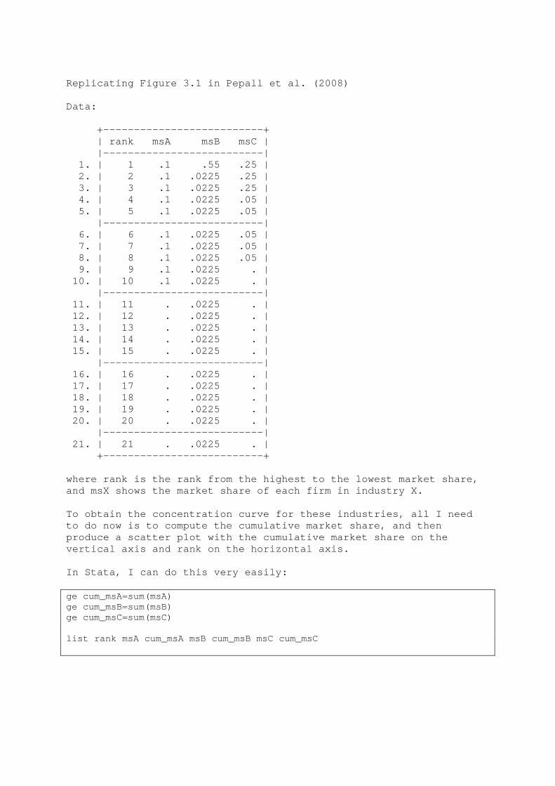
Replicating Figure 3.1 in Pepall et al. (2008) Data: +--------------------------+ | rank msA msB msC | |--------------------------| 1. | 1 .1 .55 .25 | 2. | 2 .1 .0225 .25 | 3. | 3 .1 .0225 .25 | 4. | 4 .1 .0225 .05 | 5. | 5 .1 .0225 .05 | |--------------------------| 6. | 6 .1 .0225 .05 | 7. | 7 .1 .0225 .05 | 8. | 8 .1 .0225 .05 | 9. | 9 .1 .0225 . | 10. | 10 .1 .0225 . | |--------------------------| 11. | 11 . .0225 . | 12. | 12 . .0225 . | 13. | 13 . .0225 . | 14. | 14 . .0225 . | 15. | 15 . .0225 . | |--------------------------| 16. | 16 . .0225 . | 17. | 17 . .0225 . | 18. | 18 . .0225 . | 19. | 19 . .0225 . | 20. | 20 . .0225 . | |--------------------------| 21. | 21 . .0225 . | +--------------------------+ where rank is the rank from the highest to the lowest market share, and msX shows the market share of each firm in industry X. To obtain the concentration curve for these industries, all I need to do now is to compute the cumulative market share, and then produce a scatter plot with the cumulative market share on the vertical axis and rank on the horizontal axis. In Stata, I can do this very easily: ge cum_msA=sum(msA) ge cum_msB=sum(msB) ge cum_msC=sum(msC) list rank msA cum_msA msB cum_msB msC cum_msC

+---------------------------------------------------------+ | rank msA cum_msA msB cum_msB msC cum_msC | |---------------------------------------------------------| 1. | 1 .1 .1 .55 .55 .25 .25 | 2. | 2 .1 .2 .0225 .5725 .25 .5 | 3. | 3 .1 .3 .0225 .595 .25 .75 | 4. | 4 .1 .4 .0225 .6175 .05 .8 | 5. | 5 .1 .5 .0225 .64 .05 .85 | |---------------------------------------------------------| 6. | 6 .1 .6 .0225 .6625 .05 .9 | 7. | 7 .1 .7 .0225 .685 .05 .95 | 8. | 8 .1 .8 .0225 .7075 .05 1 | 9. | 9 .1 .9 .0225 .73 . 1 | 10. | 10 .1 1 .0225 .7525 . 1 | |---------------------------------------------------------| 11. | 11 . 1 .0225 .775 . 1 | 12. | 12 . 1 .0225 .7975 . 1 | 13. | 13 . 1 .0225 .8200001 . 1 | 14. | 14 . 1 .0225 .8425 . 1 | 15. | 15 . 1 .0225 .865 . 1 | |---------------------------------------------------------| 16. | 16 . 1 .0225 .8875 . 1 | 17. | 17 . 1 .0225 .91 . 1 | 18. | 18 . 1 .0225 .9325 . 1 | 19. | 19 . 1 .0225 .955 . 1 | 20. | 20 . 1 .0225 .9775 . 1 | |---------------------------------------------------------| 21. | 21 . 1 .0225 1 . 1 | +---------------------------------------------------------+ To get the graph, I tell Stata the following: label var cum_msA "Market A" label var cum_msB "Market B" label var cum_msC "Market C" scatter cum_msA cum_msB cum_msC rank, s(i i i) c(l l l) Result:

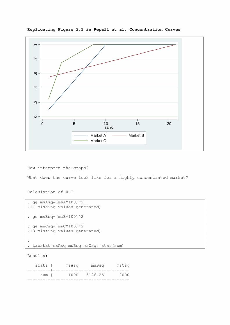
Replicating Figure 3.1 in Pepall et al. Concentration Curves

0.2

.4.6

.81

0 5 10 15 20rank

Market A Market BMarket C

How interpret the graph? What does the curve look like for a highly concentrated market? Calculation of HHI . ge msAsq=(msA*100)^2 (11 missing values generated) . ge msBsq=(msB*100)^2 . ge msCsq=(msC*100)^2 (13 missing values generated) . . tabstat msAsq msBsq msCsq, stat(sum) Results: stats | msAsq msBsq msCsq ---------+------------------------------ sum | 1000 3126.25 2000 ----------------------------------------

Concentration indices

� Concentration curves are useful but sometimes it is easier to interpret "a number" than eyeballing

lots of graphs.

� A common concentration index is the concentration ratio, CRn, de�ned as the total market

share of the top n �rms. The most common choice is to set n = 4:

� Note that the CR4 is easy to read o¤ the concentration curve (revisit Fig. 3.1 in Pepall et al.)

� Clearly CRn contains less information than the concentration curve, but arguably it is easier to

"use".

� An alternative to CRn that attempts to re�ect more fully the information in the concentration

curve is the Her�ndahl-Hirschman Index (HHI). For a market (or industry) with N �rms, this

is de�ned as follows:

HHI =NXi=1

s2i ;

where si is the market share of the ith �rm.

� What�s the HHI for a monopolist?

� What�s the HHI for a �rm in a perfectly competitive market?

� [Compute HHI for "data" underlying Fig 3.1]

� Implementation: What is a market? See lecture 2. Rarely clear-cut answer. If the de�nition of the

market is ambiguous, then clearly our measures of concentration will be open to criticism as well.

� Economic/statistical view: Products that are "closely substitutable" arguably should belong to

the same market. A useful statistical measure of the degree of substitutability is provided by the

cross-price elasticity of demand:

�ij =@qi@pj

pjqi;

20

measuring the response in demand for product i resulting from a change in the price of product j.

In practice, however, other criteria are often used - see Section 3.1.1 in Pepall et al.

5.2. Measuring market power

� We have seen how summary statistics such as the concentration ratio or the HHI index can be used

to describe the structure of a market. However, it is important to realize that a particular structure

does not necessarily imply a particular market outcome.

� For example, suppose there are only 2 or 3 �rms in the market. The HHI will indicate concentration

in the market is high. But can we be sure that market outcomes are ine¢ cient as a result? The

answer is not straightforward - as we shall see later in the course, markets with just 2 or 3 �rms

may come quite close to duplicating the competitive (e¢ cient) outcome.

� The implication is that if we want to say something about market outcomes, we had better look at

more direct measures of market outcomes.

� We are often interested in learning whether �rms in a particular market actually exercise market

power. One common summary statistic that can be used to this end is the Lerner index, de�ned

as follows:

LI =P �MC

P;

where P;MC denote price and marginal cost. Thus the Lerner index measures the discrepancy

between price and marginal cost. We saw above that, for a monopolist, the following �rst-order

condition applies:

@P (q)

@qq + P (q)� @C (q)

@q= 0�

@P (q)

@q

q

P (q)+ 1

�P (q) =

@C (q)

@q��1�+ 1

�P (q) =

@C (q)

@q�� � 1�

�P (q) =

@C (q)

@q;

21

hence

P =MC�

� � 1 ;

and

P �MC = MC

��

� � 1 � 1�

P �MC = MC

�1

� � 1

�;

and so

LI � P �MCP

=MC

�1

��1

�MC �

��1

LI =1

�:

Recall that � is the price elasticity of demand: a very high value of � implies a very elastic demand

curve, i.e. a very �at demand curve, and thus a low Lerner index. As � ! 1, as will be the case

under perfect competition, LI ! 0 (recall the demand curve from the point of view of the �rm is

�at under perfect competition).

� The greater is the Lerner Index, the farther the market outcome lies from the competitive case -

and the more market power is being exploited. In this sense, the Lerner Index is a direct indication

of the extent of market competition.

� Practical problems:

�How de�ne your market?

�Averaging over several �rms in the market - e.g.

LI = LI =P �

PNi=1 siMCiP

;

22

where si is the market share of the ith �rm and N is the total number of �rms in the market

(note that the price is common across �rms).

�Not straightforward to measure marginal costs. One popular solution is to multiply both the

numerator and the denominator by output:

LI =PQ�MC �Q

PQ=pro�tsales

:

6. Empirical Application: The Staples Case

� Reference: Ashenfelter et al. (2005). "Econometric Methods in Staples".

� The methods reviewed in the previous section are often used to describe the structure of the

market.

� Equipped with summary measures of the market structure (e.g. degree of concentration; number of

competitors etc.), we can ask how these variables correlate with outcomes of interest. There

are many possible reasons why such an analysis might be of interest. In this section we look in

detail how empirical analysis of the relationship between market power and pricing was used in

a court case concerning a proposed merger between Staples and O¢ ce Depot, in the U.S. in the

1990s.

� Two sides: The Federal Trade Commission (FTC) and the defendants. Econometric analysis played

an important role in the investigation and litigation of the case. The FTC argued that Staples

systematically charged its customers the least in cities in which its two main competitors were

present, and the most in cities where the competitors were not present.

� Consequently, it was argued, because the proposed merger would reduce competition, prices would

likely rise, harming consumers.

23

6.1. Background

� Prior to 1986, o¢ ce supplies in the U.S. were primarily bought from small independent stationers,

warehouse clubs and mail order �rms.

� In 1986, two o¢ ce supplies superstores (OSS) were set up in the country - Staples, located in the

Northeast; and O¢ ce Depot, in Florida. These superstores o¤ered a very wide range of o¢ ce

supplies to customers, known as "one-stop shopping".

� By the end of 1996, there were 3 strong OSS competitors in the U.S. market: Staples, O¢ ce Depot;

and O¢ ceMax. They had strong regional positions, and were beginning to expand into each other�s

territories.

� Staples and Depot competed directly in 40+ cities.

� In September 1996, Staples and Depot announced they were planning to merge.

� In April 1997, the FTC voted to oppose the transaction, on the grounds that consumer welfare

would be harmed as a result of the merger.

� The FTC won a preliminary injunction (court order) against the merger in U.S. District Court in

June 1997, which resulted in Staples and Depot abandoning the transaction.

6.2. The Evidence

6.2.1. Non-econometric evidence

� A lot of the evidence used in Court revolved around pricing decisions. One report described the

result of comparison-shopping a bundle of goods at o¢ ce supplies superstores in di¤erent locations,

and it was found that prices tended to be higher in locations in which there were fewer competitors.

� The price di¤erence was thus attributed to di¤erent levels of competition.

� Figure 1: Staples prices were highest in regions where it faced no competition, and lowest in markets

where the three major players were all present.

24

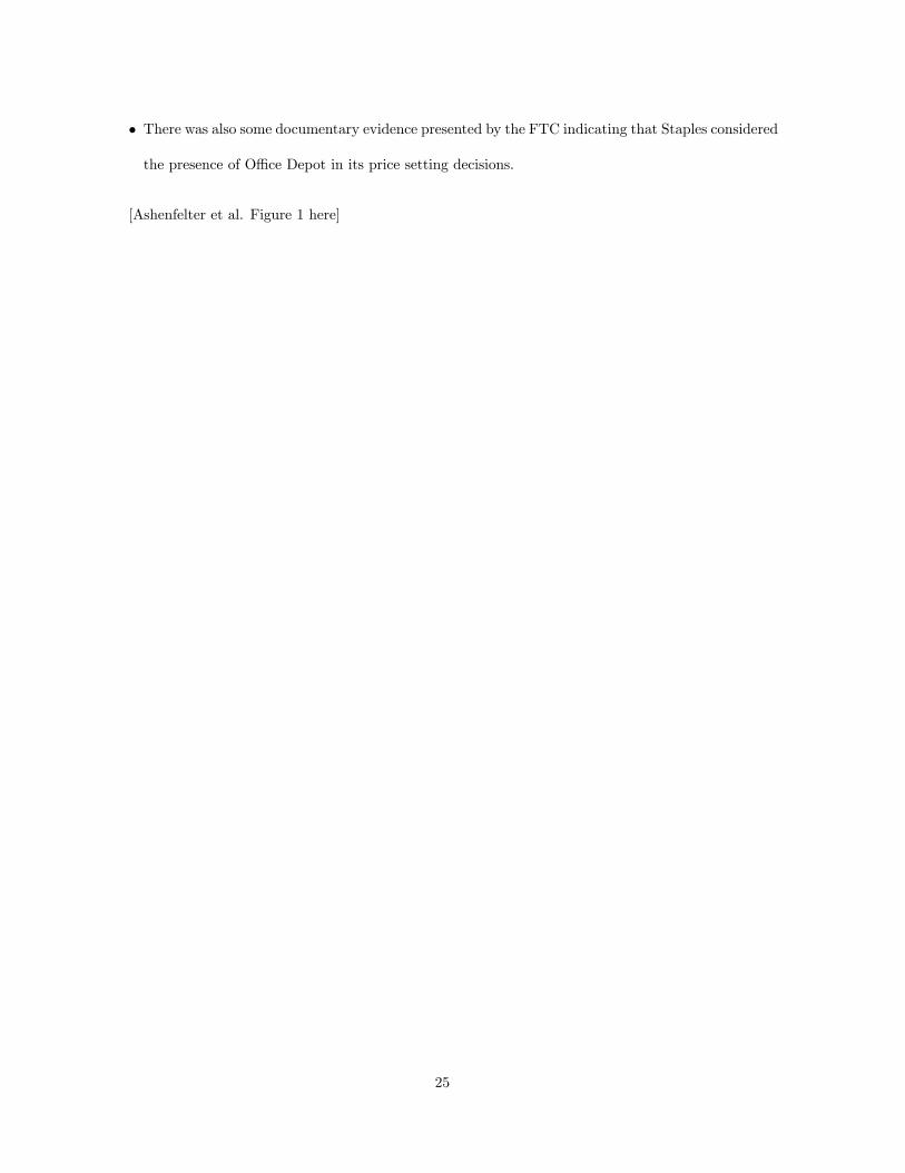
� There was also some documentary evidence presented by the FTC indicating that Staples considered

the presence of O¢ ce Depot in its price setting decisions.

[Ashenfelter et al. Figure 1 here]

25

Source: Ashenfelter et al. (2005)

6.2.2. Econometric issues

The econometric analysis focused on the impact of competition on price. One very important issue refers

to how best to estimate the impact of competition on price. The Staples case highlighted the relative

merits of:

� cross-sectional studies (which examine di¤erences in prices across a number of regions at a point

in time); and

� panel-data studies (which examine di¤erences in prices over time across the regions).

Cross sectional data. Suppose we have constructed a price index measuring the the price of some

standardized product, sold in di¤erent locations i at price pi. To investigate the e¤ect of competition on

the price, we might run a regression of the following for ·m

ln pi = �0 + �1 � competitioni +Xi + ei;

where �1 is the e¤ect of competition on price; Xi is a vector of other variables determining price (with

associated parameter vector ), �0 is the intercept, and ei is a residual.

� Clearly, to identify �1 we need a dataset in which prices as well as levels of competition di¤er across

locations.

� If we use OLS to estimate the model, we are faced with the usual problem posed by omitted

variables: maybe there are variables that we don�t observe that determine prices as well as com-

petition. For example, the following unobserved in�uences may be correlated with both prices and

entry (note: entry a¤ects competition):

�Di¤erences in marginal costs

�Di¤erences in market demand (e.g. due to high/low population)

� This might lead to omitted variables bias in the estimated coe¢ cients.

26

Panel data.

� Panel datasets exhibit a time series dimension as well as a cross-section dimension. Furthermore,

panel data contains information on the same cross section units - e.g. stores - over time. The

structure of a panel data set is as follows:

id year yr92 yr93 yr94 x1 x2

1 1992 1 0 0 8 1

1 1993 0 1 0 12 1

1 1994 0 0 1 10 1

2 1992 1 0 0 7 0

2 1993 0 1 0 5 0

2 1994 0 0 1 3 0

(...) (...) (...) (...) (...) (...) (...)

where id is the variable identifying the individual store that we follow over time; yr92, yr93 and yr94

are time dummies, constructed from the year variable; x1 is an example of a time varying variable

and x2 is an example of a time invariant variable.

� The main advantage of panel data is that it solves an omitted variables problem. Suppose our

general model is

yit = xit� + (�i + uit) ;

t = 1; 2; :::; T , where we observe yit and xit; and �i; uit are not observed. Our goal is to estimate

the parameter vector �. xit is a 1�K vector of regressors, and � is a K � 1 vector of parameters

to be estimated.

� Our problem is that we do not observe �i, which is constant over time for each individual store

(hence no t subscript) but varies across stores. Hence if we estimate the model in levels using OLS

then �i will go into the error term:

vOLSit = �i + uit:

27

Consequently, if �i is correlated with our explanatory variables, the OLS estimates will be biased.

� There are several di¤erent panel data estimators available to applied researchers. The most common

one is known as the Fixed E¤ects (FE) estimator (orWithin Estimator).

� Our general model:

yit = xit� + (�i + uit) ; t = 1; 2; :::T ; i = 1; 2; :::; N; (6.1)

where I have put �i + uit within parentheses to emphasise that these terms are unobserved.

� Assumptions about unobserved terms:

�Assumption 1.1: �i freely correlated with xit

�Assumption 1.2: E (xituis) = 0 for s = 1; 2; :::; T (strict exogeneity)

� Note that strict exogeneity rules out feedback from past uis shocks to current xit. One impli-

cation is that FE will not yield consistent estimates if xit contains lagged dependent variables

(yi;t�1; yi;t�2; :::).

� When N is large and T is small, the assumption of strict exogeneity is crucial for the FE estimator

to be consistent. In contrast, if T ! 1, strict exogeneity is not crucial Usually in empirical IO,

we have large N small T .

� If the assumption that E (xituis) = 0 for s = 1; 2; :::; T , does not hold, we may be able to use

instruments to get consistent estimates.

To see how the FE estimator solves the endogeneity problem that would contaminate the OLS esti-

mates, begin by taking the average of (6.1) for each individual - this gives

�yi = �xi� + (�i + �ui) ; i = 1; 2; :::; N; (6.2)

28

where �yi =�PT

t=1 yit

�=T , and so on.1 Now subtract (6.2) from (6.1):

yit � �yi = (xit � �xi)� + (�i � �i + uit � �ui) ;

yit � �yi = (xit � �xi)� + (uit � �ui) ;

which we write as

�yit = �xit� + �uit; t = 1; 2; :::T ; i = 1; 2; :::; N; (6.3)

where �yit is the time-demeaned data (and similarly for �xit and �uit).

This transformation of the original equation, known as the within transformation, has eliminated

�i from the equation.

� Hence, we can estimate � consistently by using OLS on (6.3). This is called theWithin estimator

or the Fixed E¤ects estimator.

� You now see why this estimator requires strict exogeneity: the equation residual in (6.3) contains

all realized residuals ui1; ui2; :::; uiT (since these enter �uit) whereas the vector of transformed ex-

planatory variables contains all realized values of the explanatory variables xi1; xi2; :::; xiT (since

these enter �xi). Hence we need E (xituis) = 0 for s = 1; 2; :::; T; or there will be endogeneity bias

if we estimate (6.3) using OLS.

� In Stata, we obtain FE estimates from the �xtreg�command if we use the option �fe�, e.g.

� xtreg yvar xvar, i(�rm) fe

� Rather than time demeaning the data, couldn�t we just estimate (6.1) by including one dummy

variable for each store? Indeed we could, and it turns out that this is exactly the same estimator

as the within estimator. If your N is large, so that you have a large number of dummy variables,

this may not be a very practical approach however.

1Without loss of generality, the exposition here assumes that T is constant across individuals, i.e. that the panel isbalanced.

29

� The panel data model used by Ashenfelter et al. is written

ln pit = �i + �1 � competitionit +Xit + eit;

where �i is the store �xed e¤ect. To obtain FE estimates, we can either do the within transformation

described above, or include N dummy variables - both procedures give the same results.

� If the omitted variables that we worried about when discussing the cross-sectional approach are

captured by �i then the FE approach solves the omitted variables problem.

� Note: You must have time series variation in prices and in the competition variable, otherwise

you cannot identify �1 by means of the FE approach. To see this, suppose your model is

ln pit = �i + �1 � competitioni +Xit + eit;

i.e. competition now doesn�t have a time subscript, indicating that it does not change over time -

similar to the variable x2 in my little example above of the structure of a panel dataset. Now do

the within transformation:

ln pit � ln pi = (�i � �i) + �1

� (competitioni � competitioni)

+�Xit �Xi

� + �eit

ln pit � ln pi =�Xit �Xi

� + �eit;

and you see that the competition term has vanished. Hence you can�t identify �1 using this ap-

proach.

� This can be a problem in applications such as this one, if entry and exit are rare events (implying

that competition stays the same in most cases).

30

Cross-Section vs. Panel Data: Use cross-section approach if

� � you don�t have panel data; or

� you have panel data but there is little entry or exit (so that your competition variable is

approximately constant over time)

Otherwise always consider the results from panel data estimators.

6.2.3. Econometric Analysis: Staples

� Economists on both sides tried to determine: how much would Staples price increase in markets

where Staples and O¢ ce Depot currently compete, if all O¢ ce Depot stores were converted to

Staples stores?

� You have already seen preliminary evidence in Figure 1 that prices are higher with less superstore

competition.

� The FTC computed a price increase of 8.6%

� The defendants computed a price increase of 1.1%

� Why did the two sides come up with such di¤erent estimates? To this question we now turn.

Data.

� The price variable was an indexed constructed from prices of products in individual OSS outlets

over time:

ln pit =Xk

!k ln pitk;

where !k is a revenue weight, k = 1; :::; 4 denotes four types of products of varying price sensitivity,

and

ln pitk =Xj2k

wjpitj ;

31

where wj is a quantity weight and pitj is the price of the j:th item at the i:th store at time t. About

7,000 di¤erent products were considered. Both sides used this price variable.

� The competition variable measured the local presence of rival OSS. Here the two sides di¤ered.

� Defendants: E¤ect of store i�s competitor depends on its distance from i:

ln pit = �i +Xt

t +X

[�1zD5it + �2zD10it + �3zD20it]

+X[�4z ln store5it + �5z ln store10it

+�6z ln store20it] + eit;

where:

� storeXit is the number of stores of retailer z within X miles of store i, at time t

�DXit is a dummy variable = 1 if retailer z does not have a store within X miles of store i, at

time t

�Parameters di¤er by z (di¤erent e¤ects for di¤erent retailers); includes retailer of store i in

the z�s in order to allow for market power e¤ects.

� FTC: Each rival store within a city had the same e¤ect regardless of distance:

ln pit = �i +Xt

t +X

�1zDzit +X

�2z ln storezit + eit

where

�Dzit is a dummy variable = 1 if at time t retailer z does not have a store in the city where

store i is located

� ln storezit is the number retailer z�s stores in the city at time t.

Which side is correct? Depends on how the retailers see the local market.

32

� If retailers see the whole city as a single market then the FTC model is better. If distance matter,

then clearly the defendants�model is better.

� Both sides use a �xed e¤ects approach, in which each individual store is tracked over time (i.e.

there are i = 1; 2; :::N stores in the dataset). They chose this approach because they were concerned

a cross-sectional approach could lead to serious omitted variable problems.

� Results: The estimated price e¤ects from the two models are very di¤erent. The FTC model gives

much higher price e¤ects - compare Model 5 (FTC) and Model 2 (defendants) in Table 1.

[Insert Table 1 here]

33

Source: Ashenfelter et al. (2005)

Defendants FTCInclude both

California included

Further comments.

� The results are sensitive to whether or not California is included in the sample. If California is

included, the price e¤ect is much greater than if it is not. Column 7.

� Recall we discussed brie�y the assumption underlying the FE estimator that the explanatory vari-

ables must be strictly exogenous (assumption 1.2 above). Thus, we have to believe that entry

and exit decisions are exogenous. However, these decisions may well be depend on Staples�price

setting, in which case competition is an endogenous variable. This problem can be addressed by

using an IV approach.

� There may be competition e¤ects on non-price variables, e.g. service levels. A more complete

analysis of competition would take such e¤ects into account.

34