advanced calculus sv
TRANSCRIPT
One Variable Advanced Calculus
Kenneth Kuttler
November 29, 2012

2

Contents
1 Introduction 7
2 The Real And Complex Numbers 92.1 The Number Line And Algebra Of The Real Numbers . . . . . . . . . . 92.2 Exercises . . . . . . . . . . . . . . . . . . . . . . . . . . . . . . . . . . . 132.3 Set Notation . . . . . . . . . . . . . . . . . . . . . . . . . . . . . . . . . 142.4 Order . . . . . . . . . . . . . . . . . . . . . . . . . . . . . . . . . . . . . 152.5 Exercises . . . . . . . . . . . . . . . . . . . . . . . . . . . . . . . . . . . 192.6 The Binomial Theorem . . . . . . . . . . . . . . . . . . . . . . . . . . . 202.7 Well Ordering Principle And Archimedian Property . . . . . . . . . . . 212.8 Exercises . . . . . . . . . . . . . . . . . . . . . . . . . . . . . . . . . . . 242.9 Completeness of R . . . . . . . . . . . . . . . . . . . . . . . . . . . . . . 272.10 Exercises . . . . . . . . . . . . . . . . . . . . . . . . . . . . . . . . . . . 282.11 The Complex Numbers . . . . . . . . . . . . . . . . . . . . . . . . . . . . 312.12 Exercises . . . . . . . . . . . . . . . . . . . . . . . . . . . . . . . . . . . 33
3 Set Theory 353.1 Basic Definitions . . . . . . . . . . . . . . . . . . . . . . . . . . . . . . . 353.2 The Schroder Bernstein Theorem . . . . . . . . . . . . . . . . . . . . . . 373.3 Equivalence Relations . . . . . . . . . . . . . . . . . . . . . . . . . . . . 403.4 Exercises . . . . . . . . . . . . . . . . . . . . . . . . . . . . . . . . . . . 41
4 Functions And Sequences 434.1 General Considerations . . . . . . . . . . . . . . . . . . . . . . . . . . . . 434.2 Sequences . . . . . . . . . . . . . . . . . . . . . . . . . . . . . . . . . . . 464.3 Exercises . . . . . . . . . . . . . . . . . . . . . . . . . . . . . . . . . . . 464.4 Worked Exercises . . . . . . . . . . . . . . . . . . . . . . . . . . . . . . . 484.5 The Limit Of A Sequence . . . . . . . . . . . . . . . . . . . . . . . . . . 504.6 The Nested Interval Lemma . . . . . . . . . . . . . . . . . . . . . . . . . 544.7 Exercises . . . . . . . . . . . . . . . . . . . . . . . . . . . . . . . . . . . 554.8 Worked Exercises . . . . . . . . . . . . . . . . . . . . . . . . . . . . . . . 564.9 Sequential Compactness . . . . . . . . . . . . . . . . . . . . . . . . . . . 58
4.9.1 Sequential Compactness . . . . . . . . . . . . . . . . . . . . . . . 584.9.2 Closed And Open Sets . . . . . . . . . . . . . . . . . . . . . . . . 58
4.10 Exercises . . . . . . . . . . . . . . . . . . . . . . . . . . . . . . . . . . . 614.11 Worked Exercises . . . . . . . . . . . . . . . . . . . . . . . . . . . . . . . 634.12 Cauchy Sequences And Completeness . . . . . . . . . . . . . . . . . . . 66
4.12.1 Decimals . . . . . . . . . . . . . . . . . . . . . . . . . . . . . . . 694.12.2 lim sup and lim inf . . . . . . . . . . . . . . . . . . . . . . . . . . 704.12.3 Shrinking Diameters . . . . . . . . . . . . . . . . . . . . . . . . . 73
4.13 Exercises . . . . . . . . . . . . . . . . . . . . . . . . . . . . . . . . . . . 73
3

4 CONTENTS
4.14 Worked Exercises . . . . . . . . . . . . . . . . . . . . . . . . . . . . . . . 76
5 Infinite Series Of Numbers 815.1 Basic Considerations . . . . . . . . . . . . . . . . . . . . . . . . . . . . . 815.2 Exercises . . . . . . . . . . . . . . . . . . . . . . . . . . . . . . . . . . . 865.3 Worked Exercises . . . . . . . . . . . . . . . . . . . . . . . . . . . . . . . 885.4 More Tests For Convergence . . . . . . . . . . . . . . . . . . . . . . . . . 91
5.4.1 Convergence Because Of Cancellation . . . . . . . . . . . . . . . 915.4.2 Ratio And Root Tests . . . . . . . . . . . . . . . . . . . . . . . . 92
5.5 Double Series . . . . . . . . . . . . . . . . . . . . . . . . . . . . . . . . . 945.6 Exercises . . . . . . . . . . . . . . . . . . . . . . . . . . . . . . . . . . . 995.7 Worked Exercises . . . . . . . . . . . . . . . . . . . . . . . . . . . . . . . 101
6 Continuous Functions 1036.1 Continuity And The Limit Of A Sequence . . . . . . . . . . . . . . . . . 1096.2 Exercises . . . . . . . . . . . . . . . . . . . . . . . . . . . . . . . . . . . 1096.3 Worked Exercises . . . . . . . . . . . . . . . . . . . . . . . . . . . . . . . 1116.4 The Extreme Values Theorem . . . . . . . . . . . . . . . . . . . . . . . . 1126.5 The Intermediate Value Theorem . . . . . . . . . . . . . . . . . . . . . . 1136.6 Exercises . . . . . . . . . . . . . . . . . . . . . . . . . . . . . . . . . . . 1156.7 Worked Exercises . . . . . . . . . . . . . . . . . . . . . . . . . . . . . . . 1166.8 Uniform Continuity . . . . . . . . . . . . . . . . . . . . . . . . . . . . . . 1176.9 Exercises . . . . . . . . . . . . . . . . . . . . . . . . . . . . . . . . . . . 1186.10 Worked Exercises . . . . . . . . . . . . . . . . . . . . . . . . . . . . . . . 1196.11 Sequences And Series Of Functions . . . . . . . . . . . . . . . . . . . . . 1216.12 Sequences Of Polynomials, Weierstrass Approximation . . . . . . . . . . 1246.13 Exercises . . . . . . . . . . . . . . . . . . . . . . . . . . . . . . . . . . . 1276.14 Worked Exercises . . . . . . . . . . . . . . . . . . . . . . . . . . . . . . . 128
7 The Derivative 1317.1 Limit Of A Function . . . . . . . . . . . . . . . . . . . . . . . . . . . . . 1317.2 Exercises . . . . . . . . . . . . . . . . . . . . . . . . . . . . . . . . . . . 1367.3 Worked Exercises . . . . . . . . . . . . . . . . . . . . . . . . . . . . . . . 1377.4 The Definition Of The Derivative . . . . . . . . . . . . . . . . . . . . . . 1387.5 Continuous And Nowhere Differentiable . . . . . . . . . . . . . . . . . . 1437.6 Finding The Derivative . . . . . . . . . . . . . . . . . . . . . . . . . . . 1457.7 Mean Value Theorem And Local Extreme Points . . . . . . . . . . . . . 1477.8 Exercises . . . . . . . . . . . . . . . . . . . . . . . . . . . . . . . . . . . 1487.9 Worked Exercises . . . . . . . . . . . . . . . . . . . . . . . . . . . . . . . 1517.10 Mean Value Theorem . . . . . . . . . . . . . . . . . . . . . . . . . . . . . 1537.11 Exercises . . . . . . . . . . . . . . . . . . . . . . . . . . . . . . . . . . . 1557.12 Worked Exercises . . . . . . . . . . . . . . . . . . . . . . . . . . . . . . . 1577.13 Derivatives Of Inverse Functions . . . . . . . . . . . . . . . . . . . . . . 1587.14 Derivatives And Limits Of Sequences . . . . . . . . . . . . . . . . . . . . 1607.15 Exercises . . . . . . . . . . . . . . . . . . . . . . . . . . . . . . . . . . . 1617.16 Worked Exercises . . . . . . . . . . . . . . . . . . . . . . . . . . . . . . . 163
8 Power Series 1698.1 Functions Defined In Terms Of Series . . . . . . . . . . . . . . . . . . . 1698.2 Operations On Power Series . . . . . . . . . . . . . . . . . . . . . . . . . 1718.3 The Special Functions Of Elementary Calculus . . . . . . . . . . . . . . 173
8.3.1 The Functions, sin, cos, exp . . . . . . . . . . . . . . . . . . . . . 1738.3.2 ln And logb . . . . . . . . . . . . . . . . . . . . . . . . . . . . . . 178

CONTENTS 5
8.4 The Binomial Theorem . . . . . . . . . . . . . . . . . . . . . . . . . . . 1808.5 Exercises . . . . . . . . . . . . . . . . . . . . . . . . . . . . . . . . . . . 1828.6 Worked Exercises . . . . . . . . . . . . . . . . . . . . . . . . . . . . . . . 1858.7 L’Hopital’s Rule . . . . . . . . . . . . . . . . . . . . . . . . . . . . . . . 187
8.7.1 Interest Compounded Continuously . . . . . . . . . . . . . . . . 1918.8 Exercises . . . . . . . . . . . . . . . . . . . . . . . . . . . . . . . . . . . 1918.9 Multiplication Of Power Series . . . . . . . . . . . . . . . . . . . . . . . 1938.10 Exercises . . . . . . . . . . . . . . . . . . . . . . . . . . . . . . . . . . . 1958.11 Worked Exercises . . . . . . . . . . . . . . . . . . . . . . . . . . . . . . . 1988.12 Worked Exercises . . . . . . . . . . . . . . . . . . . . . . . . . . . . . . . 1998.13 The Fundamental Theorem Of Algebra . . . . . . . . . . . . . . . . . . . 2018.14 Some Other Theorems . . . . . . . . . . . . . . . . . . . . . . . . . . . . 203
9 The Riemann And Riemann Stieltjes Integrals 2079.1 The Darboux Stieltjes Integral . . . . . . . . . . . . . . . . . . . . . . . 207
9.1.1 Upper And Lower Darboux Stieltjes Sums . . . . . . . . . . . . . 2079.2 Exercises . . . . . . . . . . . . . . . . . . . . . . . . . . . . . . . . . . . 211
9.2.1 Functions Of Darboux Integrable Functions . . . . . . . . . . . . 2139.2.2 Properties Of The Integral . . . . . . . . . . . . . . . . . . . . . 2159.2.3 Fundamental Theorem Of Calculus . . . . . . . . . . . . . . . . . 219
9.3 Exercises . . . . . . . . . . . . . . . . . . . . . . . . . . . . . . . . . . . 2229.4 The Riemann Stieltjes Integral . . . . . . . . . . . . . . . . . . . . . . . 225
9.4.1 Change Of Variables . . . . . . . . . . . . . . . . . . . . . . . . . 2299.4.2 A Simple Procedure For Finding Integrals . . . . . . . . . . . . . 2319.4.3 General Riemann Stieltjes Integrals . . . . . . . . . . . . . . . . 2329.4.4 Stirling’s Formula . . . . . . . . . . . . . . . . . . . . . . . . . . 237
9.5 Exercises . . . . . . . . . . . . . . . . . . . . . . . . . . . . . . . . . . . 240
10 Fourier Series 24910.1 The Complex Exponential . . . . . . . . . . . . . . . . . . . . . . . . . . 24910.2 Definition And Basic Properties . . . . . . . . . . . . . . . . . . . . . . . 24910.3 The Riemann Lebesgue Lemma . . . . . . . . . . . . . . . . . . . . . . . 25310.4 Dini’s Criterion For Convergence . . . . . . . . . . . . . . . . . . . . . . 25710.5 Integrating And Differentiating Fourier Series . . . . . . . . . . . . . . . 26010.6 Ways Of Approximating Functions . . . . . . . . . . . . . . . . . . . . . 264
10.6.1 Uniform Approximation With Trig. Polynomials . . . . . . . . . 26510.6.2 Mean Square Approximation . . . . . . . . . . . . . . . . . . . . 267
10.7 Exercises . . . . . . . . . . . . . . . . . . . . . . . . . . . . . . . . . . . 270
11 The Generalized Riemann Integral 27711.1 Definitions And Basic Properties . . . . . . . . . . . . . . . . . . . . . . 27711.2 Integrals Of Derivatives . . . . . . . . . . . . . . . . . . . . . . . . . . . 28711.3 Exercises . . . . . . . . . . . . . . . . . . . . . . . . . . . . . . . . . . . 289
A Construction Of Real Numbers 293Copyright c⃝ 2007,

6 CONTENTS

Introduction
The difference between advanced calculus and calculus is that all the theorems areproved completely and the role of plane geometry is minimized. Instead, the notion ofcompleteness is of preeminent importance. Silly gimmicks are of no significance at all.Routine skills involving elementary functions and integration techniques are supposed tobe mastered and have no place in advanced calculus which deals with the fundamentalissues related to existence and meaning. This is a subject which places calculus as partof mathematics and involves proofs and definitions, not algorithms and busy work.
An orderly development of the elementary functions is included but it is assumed thereader is familiar enough with these functions to use them in problems which illustratesome of the ideas presented.
7

8 INTRODUCTION
The Real And ComplexNumbers
2.1 The Number Line And Algebra Of The Real Num-bers
To begin with, consider the real numbers, denoted by R, as a line extending infinitely farin both directions. In this book, the notation, ≡ indicates something is being defined.Thus the integers are defined as
Z ≡{· · · − 1, 0, 1, · · · } ,
the natural numbers,N ≡ {1, 2, · · · }
and the rational numbers, defined as the numbers which are the quotient of two integers.
Q ≡{mn
such that m,n ∈ Z, n = 0}
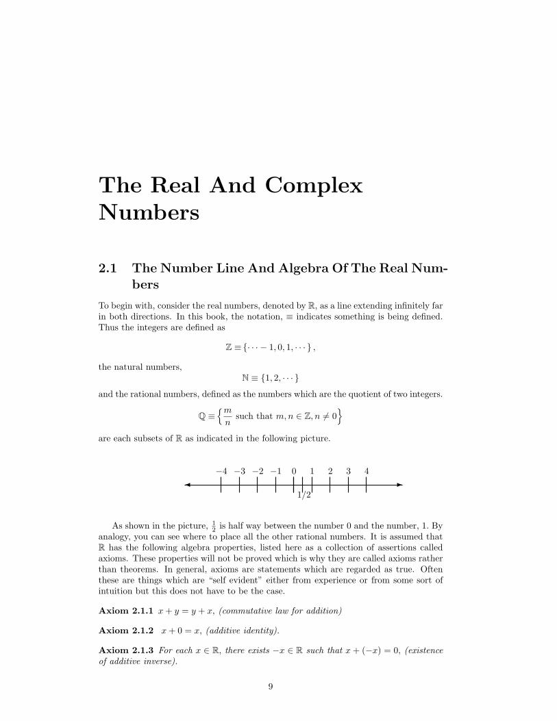
are each subsets of R as indicated in the following picture.
0
1/2
1 2 3 4−1−2−3−4-�
As shown in the picture, 12 is half way between the number 0 and the number, 1. By
analogy, you can see where to place all the other rational numbers. It is assumed thatR has the following algebra properties, listed here as a collection of assertions calledaxioms. These properties will not be proved which is why they are called axioms ratherthan theorems. In general, axioms are statements which are regarded as true. Oftenthese are things which are “self evident” either from experience or from some sort ofintuition but this does not have to be the case.
Axiom 2.1.1 x+ y = y + x, (commutative law for addition)
Axiom 2.1.2 x+ 0 = x, (additive identity).
Axiom 2.1.3 For each x ∈ R, there exists −x ∈ R such that x+ (−x) = 0, (existenceof additive inverse).
9

10 THE REAL AND COMPLEX NUMBERS
Axiom 2.1.4 (x+ y) + z = x+ (y + z) , (associative law for addition).
Axiom 2.1.5 xy = yx, (commutative law for multiplication).
Axiom 2.1.6 (xy) z = x (yz) , (associative law for multiplication).
Axiom 2.1.7 1x = x, (multiplicative identity).
Axiom 2.1.8 For each x = 0, there exists x−1 such that xx−1 = 1.(existence of multi-plicative inverse).
Axiom 2.1.9 x (y + z) = xy + xz.(distributive law).
These axioms are known as the field axioms and any set (there are many othersbesides R) which has two such operations satisfying the above axioms is called a field.Division and subtraction are defined in the usual way by x− y ≡ x+ (−y) and x/y ≡x(y−1
). It is assumed that the reader is completely familiar with these axioms in the
sense that he or she can do the usual algebraic manipulations taught in high school andjunior high algebra courses. The axioms listed above are just a careful statement ofexactly what is necessary to make the usual algebraic manipulations valid. A word ofadvice regarding division and subtraction is in order here. Whenever you feel a littleconfused about an algebraic expression which involves division or subtraction, think ofdivision as multiplication by the multiplicative inverse as just indicated and think ofsubtraction as addition of the additive inverse. Thus, when you see x/y, think x
(y−1
)and when you see x − y, think x + (−y) . In many cases the source of confusion willdisappear almost magically. The reason for this is that subtraction and division do notsatisfy the associative law. This means there is a natural ambiguity in an expressionlike 6 − 3 − 4. Do you mean (6− 3) − 4 = −1 or 6 − (3− 4) = 6 − (−1) = 7? Itmakes a difference doesn’t it? However, the so called binary operations of addition andmultiplication are associative and so no such confusion will occur. It is conventional tosimply do the operations in order of appearance reading from left to right. Thus, if yousee 6− 3− 4, you would normally interpret it as the first of the above alternatives.
In doing algebra, the following theorem is important and follows from the aboveaxioms. The reasoning which demonstrates this assertion is called a proof. Proofs anddefinitions are very important in mathematics because they are the means by which“truth” is determined. In mathematics, something is “true” if it follows from axiomsusing a correct logical argument. Truth is not determined on the basis of experimentor opinions and it is this which makes mathematics useful as a language for describingcertain kinds of reality in a precise manner.1 It is also the definitions and proofs whichmake the subject of mathematics intellectually worth while. Take these away and itbecomes a gray wasteland filled with endless tedium and meaningless manipulations.
In the first part of the following theorem, the claim is made that the additive inverseand the multiplicative inverse are unique. This means that for a given number, only onenumber has the property that it is an additive inverse and that, given a nonzero number,only one number has the property that it is a multiplicative inverse. The significanceof this is that if you are wondering if a given number is the additive inverse of a givennumber, all you have to do is to check and see if it acts like one.
Theorem 2.1.10 The above axioms imply the following.
1. The multiplicative inverse and additive inverses are unique.
1There are certainly real and important things which should not be described using mathematicsbecause it has nothing to do with these things. For example, feelings and emotions have nothing to dowith math.
2.1. THE NUMBER LINE AND ALGEBRA OF THE REAL NUMBERS 11
2. 0x = 0, − (−x) = x,
3. (−1) (−1) = 1, (−1)x = −x
4. If xy = 0 then either x = 0 or y = 0.
Proof:Suppose then that x is a real number and that x + y = 0 = x + z. It isnecessary to verify y = z. From the above axioms, there exists an additive inverse, −xfor x. Therefore,
−x+ 0 = (−x) + (x+ y) = (−x) + (x+ z)
and so by the associative law for addition,
((−x) + x) + y = ((−x) + x) + z
which implies0 + y = 0 + z.
Now by the definition of the additive identity, this implies y = z. You should prove themultiplicative inverse is unique.
Consider 2. It is desired to verify 0x = 0. From the definition of the additive identityand the distributive law it follows that
0x = (0 + 0)x = 0x+ 0x.
From the existence of the additive inverse and the associative law it follows
0 = (−0x) + 0x = (−0x) + (0x+ 0x)
= ((−0x) + 0x) + 0x = 0 + 0x = 0x
To verify the second claim in 2., it suffices to show x acts like the additive inverse of−x in order to conclude that − (−x) = x. This is because it has just been shown thatadditive inverses are unique. By the definition of additive inverse,
x+ (−x) = 0
and so x = − (−x) as claimed.To demonstrate 3.,
(−1) (1 + (−1)) = (−1) 0 = 0
and so using the definition of the multiplicative identity, and the distributive law,
(−1) + (−1) (−1) = 0.
It follows from 1. and 2. that 1 = − (−1) = (−1) (−1) . To verify (−1)x = −x, use 2.and the distributive law to write
x+ (−1)x = x (1 + (−1)) = x0 = 0.
Therefore, by the uniqueness of the additive inverse proved in 1., it follows (−1)x = −xas claimed.
To verify 4., suppose x = 0. Then x−1 exists by the axiom about the existence ofmultiplicative inverses. Therefore, by 2. and the associative law for multiplication,
y =(x−1x
)y = x−1 (xy) = x−10 = 0.
This proves 4. and completes the proof of this theorem.

12 THE REAL AND COMPLEX NUMBERS
Recall the notion of something raised to an integer power. Thus y2 = y × y andb−3 = 1
b3 etc.Also, there are a few conventions related to the order in which operations are per-
formed. Exponents are always done before multiplication. Thus xy2 = x(y2)and is not
equal to (xy)2. Division or multiplication is always done before addition or subtraction.
Thus x − y (z + w) = x − [y (z + w)] and is not equal to (x− y) (z + w) . Parenthesesare done before anything else. Be very careful of such things since they are a source ofmistakes. When you have doubts, insert parentheses to resolve the ambiguities.
Also recall summation notation. If you have not seen this, the following is a shortreview of this topic.
Definition 2.1.11 Let x1, x2, · · · , xm be numbers. Then
m∑j=1
xj ≡ x1 + x2 + · · ·+ xm.
Thus this symbol,∑m
j=1 xj means to take all the numbers, x1, x2, · · · , xm and add themall up. Note the use of the j as a generic variable which takes values from 1 up tom. This notation will be used whenever there are things which can be added, not justnumbers.
As an example of the use of this notation, you should verify the following.
Example 2.1.12∑6
k=1 (2k + 1) = 48.
Be sure you understand why
m+1∑k=1
xk =m∑
k=1
xk + xm+1.
As a slight generalization of this notation,
m∑j=k
xj ≡ xk + · · ·+ xm.
It is also possible to change the variable of summation.
m∑j=1
xj = x1 + x2 + · · ·+ xm
while if r is an integer, the notation requires
m+r∑j=1+r
xj−r = x1 + x2 + · · ·+ xm
and so∑m
j=1 xj =∑m+r
j=1+r xj−r.Summation notation will be used throughout the book whenever it is convenient to
do so.Another thing to keep in mind is that you often use letters to represent numbers.
Since they represent numbers, you manipulate expressions involving letters in the samemanner as you would if they were specific numbers.
Example 2.1.13 Add the fractions, xx2+y + y
x−1 .

2.2. EXERCISES 13
You add these just like they were numbers. Write the first expression as x(x−1)(x2+y)(x−1)
and the second asy(x2+y)
(x−1)(x2+y) . Then since these have the same common denominator,
you add them as follows.
x
x2 + y+
y
x− 1=
x (x− 1)
(x2 + y) (x− 1)+
y(x2 + y
)(x− 1) (x2 + y)
=x2 − x+ yx2 + y2
(x2 + y) (x− 1).
2.2 Exercises
1. Consider the expression x+ y (x+ y)− x (y − x) ≡ f (x, y) . Find f (−1, 2) .
2. Show − (ab) = (−a) b.
3. Show on the number line the effect of adding two positive numbers, x and y.
4. Show on the number line the effect of subtracting a positive number from anotherpositive number.
5. Show on the number line the effect of multiplying a number by −1.
6. Add the fractions xx2−1 + x−1
x+1 .
7. Find a formula for (x+ y)2, (x+ y)
3, and (x+ y)
4. Based on what you observe
for these, give a formula for (x+ y)8.
8. When is it true that (x+ y)n= xn + yn?
9. Find the error in the following argument. Let x = y = 1. Then xy = y2 and soxy − x2 = y2 − x2. Therefore, x (y − x) = (y − x) (y + x) . Dividing both sides by(y − x) yields x = x + y. Now substituting in what these variables equal yields1 = 1 + 1.
10. Find the error in the following argument.√x2 + 1 = x + 1 and so letting x = 2,√
5 = 3. Therefore, 5 = 9.
11. Find the error in the following. Let x = 1 and y = 2. Then 13 = 1
x+y = 1x + 1
y =
1 + 12 = 3
2 . Then cross multiplying, yields 2 = 9.
12. Simplify x2y4z−6
x−2y−1z .
13. Simplify the following expressions using correct algebra. In these expressions thevariables represent real numbers.
(a) x2y+xy2+xx
(b) x2y+xy2+xxy
(c) x3+2x2−x−2x+1
14. Find the error in the following argument. Let x = 3 and y = 1. Then 1 = 3− 2 =3− (3− 1) = x− y (x− y) = (x− y) (x− y) = 22 = 4.
15. Verify the following formulas.
(a) (x− y) (x+ y) = x2 − y2
14 THE REAL AND COMPLEX NUMBERS
(b) (x− y)(x2 + xy + y2
)= x3 − y3
(c) (x+ y)(x2 − xy + y2
)= x3 + y3
16. Find the error in the following.
xy + y
x= y + y = 2y.
Now let x = 2 and y = 2 to obtain
3 = 4
17. Show the rational numbers satisfy the field axioms. You may assume the associa-tive, commutative, and distributive laws hold for the integers.
2.3 Set Notation
A set is just a collection of things called elements. Often these are also referred to aspoints in calculus. For example {1, 2, 3, 8} would be a set consisting of the elements1,2,3, and 8. To indicate that 3 is an element of {1, 2, 3, 8} , it is customary to write3 ∈ {1, 2, 3, 8} . 9 /∈ {1, 2, 3, 8} means 9 is not an element of {1, 2, 3, 8} . Sometimes a rulespecifies a set. For example you could specify a set as all integers larger than 2. Thiswould be written as S = {x ∈ Z : x > 2} . This notation says: the set of all integers, x,such that x > 2.
If A and B are sets with the property that every element of A is an element ofB, then A is a subset of B. For example, {1, 2, 3, 8} is a subset of {1, 2, 3, 4, 5, 8} , insymbols, {1, 2, 3, 8} ⊆ {1, 2, 3, 4, 5, 8} . The same statement about the two sets may alsobe written as {1, 2, 3, 4, 5, 8} ⊇ {1, 2, 3, 8}.
The union of two sets is the set consisting of everything which is contained in at leastone of the sets, A or B. As an example of the union of two sets, {1, 2, 3, 8}∪{3, 4, 7, 8} ={1, 2, 3, 4, 7, 8} because these numbers are those which are in at least one of the two sets.In general
A ∪B ≡ {x : x ∈ A or x ∈ B} .
Be sure you understand that something which is in both A and B is in the union. It isnot an exclusive or.
The intersection of two sets, A and B consists of everything which is in both of thesets. Thus {1, 2, 3, 8} ∩ {3, 4, 7, 8} = {3, 8} because 3 and 8 are those elements the twosets have in common. In general,
A ∩B ≡ {x : x ∈ A and x ∈ B} .
When with real numbers, [a, b] denotes the set of real numbers, x, such that a ≤ x ≤ band [a, b) denotes the set of real numbers such that a ≤ x < b. (a, b) consists of the setof real numbers, x such that a < x < b and (a, b] indicates the set of numbers, x suchthat a < x ≤ b. [a,∞) means the set of all numbers, x such that x ≥ a and (−∞, a]means the set of all real numbers which are less than or equal to a. These sorts of setsof real numbers are called intervals. The two points, a and b are called endpoints ofthe interval. Other intervals such as (−∞, b) are defined by analogy to what was justexplained. In general, the curved parenthesis indicates the end point it sits next tois not included while the square parenthesis indicates this end point is included. Thereason that there will always be a curved parenthesis next to ∞ or −∞ is that theseare not real numbers. Therefore, they cannot be included in any set of real numbers.

2.4. ORDER 15
A special set which needs to be given a name is the empty set also called the null set,denoted by ∅. Thus ∅ is defined as the set which has no elements in it. Mathematicianslike to say the empty set is a subset of every set. The reason they say this is that if itwere not so, there would have to exist a set, A, such that ∅ has something in it which isnot in A. However, ∅ has nothing in it and so the least intellectual discomfort is achievedby saying ∅ ⊆ A.
If A and B are two sets, A \ B denotes the set of things which are in A but not inB. Thus
A \B ≡ {x ∈ A : x /∈ B} .
Set notation is used whenever convenient.
2.4 Order
The real numbers also have an order defined on them. This order may be definedby reference to the positive real numbers, those to the right of 0 on the number line,denoted by R+ which is assumed to satisfy the following axioms.
The sum of two positive real numbers is positive. (2.1)
The product of two positive real numbers is positive. (2.2)
For a given real number, x, one and only
one of the following alternatives
holds. Either x is positive, x equals 0 or − x is positive. (2.3)
Definition 2.4.1 x < y exactly when y+(−x) ≡ y−x ∈ R+. In the usual way,x < y is the same as y > x and x ≤ y means either x < y or x = y. The symbol ≥ isdefined similarly.
Theorem 2.4.2 The following hold for the order defined as above.
1. If x < y and y < z then x < z (Transitive law).
2. If x < y then x+ z < y + z (addition to an inequality).
3. If x ≤ 0 and y ≤ 0, then xy ≥ 0.
4. If x > 0 then x−1 > 0.
5. If x < 0 then x−1 < 0.
6. If x < y then xz < yz if z > 0, (multiplication of an inequality).
7. If x < y and z < 0, then xz > zy (multiplication of an inequality).
8. Each of the above holds with > and < replaced by ≥ and ≤ respectively except for4 and 5 in which we must also stipulate that x = 0.
9. For any x and y, exactly one of the following must hold. Either x = y, x < y, orx > y (trichotomy).
16 THE REAL AND COMPLEX NUMBERS
Proof: First consider 1, the transitive law. Suppose x < y and y < z. Why isx < z? In other words, why is z − x ∈ R+? It is because z − x = (z − y) + (y − x) andboth z − y, y − x ∈ R+. Thus by 2.1 above, z − x ∈ R+ and so z > x.
Next consider 2, addition to an inequality. If x < y why is x + z < y + z? it isbecause
(y + z) +− (x+ z) = (y + z) + (−1) (x+ z)
= y + (−1)x+ z + (−1) z= y − x ∈ R+.
Next consider 3. If x ≤ 0 and y ≤ 0, why is xy ≥ 0? First note there is nothing toshow if either x or y equal 0 so assume this is not the case. By 2.3 −x > 0 and −y > 0.Therefore, by 2.2 and what was proved about −x = (−1)x,
(−x) (−y) = (−1)2 xy ∈ R+.
Is (−1)2 = 1? If so the claim is proved. But − (−1) = (−1)2 and − (−1) = 1 because
−1 + 1 = 0.
Next consider 4. If x > 0 why is x−1 > 0? By 2.3 either x−1 = 0 or −x−1 ∈ R+.It can’t happen that x−1 = 0 because then you would have to have 1 = 0x and as wasshown earlier, 0x = 0. Therefore, consider the possibility that −x−1 ∈ R+. This can’twork either because then you would have
(−1)x−1x = (−1) (1) = −1
and it would follow from 2.2 that −1 ∈ R+. But this is impossible because if x ∈ R+,then (−1)x = −x ∈ R+ and contradicts 2.3 which states that either −x or x is in R+
but not both.Next consider 5. If x < 0, why is x−1 < 0? As before, x−1 = 0. If x−1 > 0, then as
before,−x(x−1
)= −1 ∈ R+
which was just shown not to occur.Next consider 6. If x < y why is xz < yz if z > 0? This follows because
yz − xz = z (y − x) ∈ R+
since both z and y − x ∈ R+.Next consider 7. If x < y and z < 0, why is xz > zy? This follows because
zx− zy = z (x− y) ∈ R+
by what was proved in 3.The last two claims are obvious and left for you. This proves the theorem.Note that trichotomy could be stated by saying x ≤ y or y ≤ x.
Definition 2.4.3 |x| ≡{
x if x ≥ 0,−x if x < 0.
Note that |x| can be thought of as the distance between x and 0.
Theorem 2.4.4 |xy| = |x| |y| .
Proof: You can verify this by checking all available cases. Do so.

2.4. ORDER 17
Theorem 2.4.5 The following inequalities hold.
|x+ y| ≤ |x|+ |y| , ||x| − |y|| ≤ |x− y| .
Either of these inequalities may be called the triangle inequality.
Proof: First note that if a, b ∈ R+ ∪ {0} then a ≤ b if and only if a2 ≤ b2. Here iswhy. Suppose a ≤ b. Then by the properties of order proved above,
a2 ≤ ab ≤ b2
because b2 − ab = b (b− a) ∈ R+ ∪ {0} . Next suppose a2 ≤ b2. If both a, b = 0 there isnothing to show. Assume then they are not both 0. Then
b2 − a2 = (b+ a) (b− a) ∈ R+.
By the above theorem on order, (a+ b)−1 ∈ R+ and so using the associative law,
(a+ b)−1
((b+ a) (b− a)) = (b− a) ∈ R+
Now
|x+ y|2 = (x+ y)2= x2 + 2xy + y2
≤ |x|2 + |y|2 + 2 |x| |y| = (|x|+ |y|)2
and so the first of the inequalities follows. Note I used xy ≤ |xy| = |x| |y| which followsfrom the definition.
To verify the other form of the triangle inequality,
x = x− y + y
so|x| ≤ |x− y|+ |y|
and so|x| − |y| ≤ |x− y| = |y − x|
Now repeat the argument replacing the roles of x and y to conclude
|y| − |x| ≤ |y − x| .
Therefore,||y| − |x|| ≤ |y − x| .
This proves the triangle inequality.
Example 2.4.6 Solve the inequality 2x+ 4 ≤ x− 8
Subtract 2x from both sides to yield 4 ≤ −x − 8. Next add 8 to both sides to get12 ≤ −x. Then multiply both sides by (−1) to obtain x ≤ −12. Alternatively, subtractx from both sides to get x+4 ≤ −8. Then subtract 4 from both sides to obtain x ≤ −12.
Example 2.4.7 Solve the inequality (x+ 1) (2x− 3) ≥ 0.
If this is to hold, either both of the factors, x+1 and 2x−3 are nonnegative or theyare both non-positive. The first case yields x + 1 ≥ 0 and 2x − 3 ≥ 0 so x ≥ −1 andx ≥ 3
2 yielding x ≥ 32 . The second case yields x + 1 ≤ 0 and 2x − 3 ≤ 0 which implies
x ≤ −1 and x ≤ 32 . Therefore, the solution to this inequality is x ≤ −1 or x ≥ 3
2 .
18 THE REAL AND COMPLEX NUMBERS
Example 2.4.8 Solve the inequality (x) (x+ 2) ≥ −4
Here the problem is to find x such that x2 + 2x + 4 ≥ 0. However, x2 + 2x + 4 =(x+ 1)
2+ 3 ≥ 0 for all x. Therefore, the solution to this problem is all x ∈ R.
Example 2.4.9 Solve the inequality 2x+ 4 ≤ x− 8
This is written as (−∞,−12].
Example 2.4.10 Solve the inequality (x+ 1) (2x− 3) ≥ 0.
This was worked earlier and x ≤ −1 or x ≥ 32 was the answer. In terms of set
notation this is denoted by (−∞,−1] ∪ [ 32 ,∞).
Example 2.4.11 Solve the equation |x− 1| = 2
This will be true when x − 1 = 2 or when x − 1 = −2. Therefore, there are twosolutions to this problem, x = 3 or x = −1.
Example 2.4.12 Solve the inequality |2x− 1| < 2
From the number line, it is necessary to have 2x − 1 between −2 and 2 becausethe inequality says that the distance from 2x − 1 to 0 is less than 2. Therefore, −2 <2x− 1 < 2 and so −1/2 < x < 3/2. In other words, −1/2 < x and x < 3/2.
Example 2.4.13 Solve the inequality |2x− 1| > 2.
This happens if 2x − 1 > 2 or if 2x − 1 < −2. Thus the solution is x > 3/2 orx < −1/2. Written in terms of intervals this is
(32 ,∞
)∪(−∞,− 1
2
).
Example 2.4.14 Solve |x+ 1| = |2x− 2|
There are two ways this can happen. It could be the case that x + 1 = 2x − 2 inwhich case x = 3 or alternatively, x+ 1 = 2− 2x in which case x = 1/3.
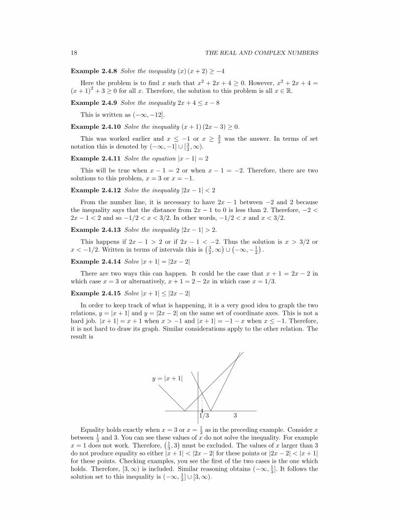
Example 2.4.15 Solve |x+ 1| ≤ |2x− 2|
In order to keep track of what is happening, it is a very good idea to graph the tworelations, y = |x+ 1| and y = |2x− 2| on the same set of coordinate axes. This is not ahard job. |x+ 1| = x+ 1 when x > −1 and |x+ 1| = −1− x when x ≤ −1. Therefore,it is not hard to draw its graph. Similar considerations apply to the other relation. Theresult is
����
����
�
@@
@@
���������
AAAAAA
1/3 3
y = |x+ 1|
Equality holds exactly when x = 3 or x = 13 as in the preceding example. Consider x
between 13 and 3. You can see these values of x do not solve the inequality. For example
x = 1 does not work. Therefore,(13 , 3)must be excluded. The values of x larger than 3
do not produce equality so either |x+ 1| < |2x− 2| for these points or |2x− 2| < |x+ 1|for these points. Checking examples, you see the first of the two cases is the one whichholds. Therefore, [3,∞) is included. Similar reasoning obtains (−∞, 13 ]. It follows thesolution set to this inequality is (−∞, 13 ] ∪ [3,∞).

2.5. EXERCISES 19
Example 2.4.16 Suppose ε > 0 is a given positive number. Obtain a number, δ > 0,such that if |x− 1| < δ, then
∣∣x2 − 1∣∣ < ε.
First of all, note∣∣x2 − 1
∣∣ = |x− 1| |x+ 1| ≤ (|x|+ 1) |x− 1| . Now if |x− 1| < 1, itfollows |x| < 2 and so for |x− 1| < 1,∣∣x2 − 1
∣∣ < 3 |x− 1| .
Now let δ = min(1, ε3
). This notation means to take the minimum of the two numbers,
1 and ε3 . Then if |x− 1| < δ,∣∣x2 − 1
∣∣ < 3 |x− 1| < 3ε
3= ε.
2.5 Exercises
1. Solve (3x+ 2) (x− 3) ≤ 0.
2. Solve (3x+ 2) (x− 3) > 0.
3. Solve x+23x−2 < 0.
4. Solvex+1x+3 < 1.
5. Solve (x− 1) (2x+ 1) ≤ 2.
6. Solve (x− 1) (2x+ 1) > 2.
7. Solve x2 − 2x ≤ 0.
8. Solve (x+ 2) (x− 2)2 ≤ 0.
9. Solve 3x−4x2+2x+2 ≥ 0.
10. Solve 3x+9x2+2x+1 ≥ 1.
11. Solve x2+2x+13x+7 < 1.
12. Solve |x+ 1| = |2x− 3| .
13. Solve |3x+ 1| < 8. Give your answer in terms of intervals on the real line.
14. Sketch on the number line the solution to the inequality |x− 3| > 2.
15. Sketch on the number line the solution to the inequality |x− 3| < 2.
16. Show |x| =√x2.
17. Solve |x+ 2| < |3x− 3| .
18. Tell when equality holds in the triangle inequality.
19. Solve |x+ 2| ≤ 8 + |2x− 4| .
20. Solve (x+ 1) (2x− 2)x ≥ 0.
21. Solve x+32x+1 > 1.
22. Solve x+23x+1 > 2.

20 THE REAL AND COMPLEX NUMBERS
23. Describe the set of numbers, a such that there is no solution to |x+ 1| = 4−|x+ a| .
24. Suppose 0 < a < b. Show a−1 > b−1.
25. Show that if |x− 6| < 1, then |x| < 7.
26. Suppose |x− 8| < 2. How large can |x− 5| be?
27. Obtain a number, δ > 0, such that if |x− 1| < δ, then∣∣x2 − 1
∣∣ < 1/10.
28. Obtain a number, δ > 0, such that if |x− 4| < δ, then |√x− 2| < 1/10.
29. Suppose ε > 0 is a given positive number. Obtain a number, δ > 0, such that if|x− 1| < δ, then |
√x− 1| < ε. Hint: This δ will depend in some way on ε. You
need to tell how.
2.6 The Binomial Theorem
Consider the following problem: You have the integers Sn = {1, 2, · · · , n} and k is aninteger no larger than n. How many ways are there to fill k slots with these integersstarting from left to right if whenever an integer from Sn has been used, it cannot bere used in any succeeding slot?
k of these slots︷ ︸︸ ︷, , , , · · · ,
This number is known as permutations of n things taken k at a time and is denotedby P (n, k). It is easy to figure it out. There are n choices for the first slot. For eachchoice for the fist slot, there remain n − 1 choices for the second slot. Thus there aren (n− 1) ways to fill the first two slots. Now there remain n− 2 ways to fill the third.Thus there are n (n− 1) (n− 2) ways to fill the first three slots. Continuing this way,you see there are
P (n, k) = n (n− 1) (n− 2) · · · (n− k + 1)
ways to do this.Now define for k a positive integer,
k! ≡ k (k − 1) (k − 2) · · · 1, 0! ≡ 1.
This is called k factorial. Thus P (k, k) = k! and you should verify that
P (n, k) =n!
(n− k)!
Now consider the number of ways of selecting a set of k different numbers from Sn. Foreach set of k numbers there are P (k, k) = k! ways of listing these numbers in order.
Therefore, denoting by
(nk
)the number of ways of selecting a set of k numbers from
Sn, it must be the case that(nk
)k! = P (n, k) =
n!
(n− k)!
Therefore, (nk
)=
n!
k! (n− k)!.

2.7. WELL ORDERING PRINCIPLE AND ARCHIMEDIAN PROPERTY 21
How many ways are there to select no numbers from Sn? Obviously one way. Note theabove formula gives the right answer in this case as well as in all other cases due to thedefinition which says 0! = 1.
Now consider the problem of writing a formula for (x+ y)nwhere n is a positive
integer. Imagine writing it like this:
n times︷ ︸︸ ︷(x+ y) (x+ y) · · · (x+ y)
Then you know the result will be sums of terms of the form akxkyn−k. What is ak? In
other words, how many ways can you pick x from k of the factors above and y fromthe other n− k. There are n factors so the number of ways to do it is(
nk
).
Therefore, ak is the above formula and so this proves the following important theoremknown as the binomial theorem.
Theorem 2.6.1 The following formula holds for any n a positive integer.
(x+ y)n=
n∑k=0
(nk
)xkyn−k.
2.7 Well Ordering Principle And Archimedian Prop-erty
Definition 2.7.1 A set is well ordered if every nonempty subset S, contains asmallest element z having the property that z ≤ x for all x ∈ S.
Axiom 2.7.2 Any set of integers larger than a given number is well ordered.
In particular, the natural numbers defined as
N ≡{1, 2, · · · }
is well ordered.The above axiom implies the principle of mathematical induction.
Theorem 2.7.3 (Mathematical induction) A set S ⊆ Z, having the property thata ∈ S and n+ 1 ∈ S whenever n ∈ S contains all integers x ∈ Z such that x ≥ a.
Proof: Let T ≡ ([a,∞) ∩ Z)\S. Thus T consists of all integers larger than or equalto a which are not in S. The theorem will be proved if T = ∅. If T = ∅ then by the wellordering principle, there would have to exist a smallest element of T, denoted as b. Itmust be the case that b > a since by definition, a /∈ T. Then the integer, b− 1 ≥ a andb − 1 /∈ S because if b − 1 ∈ S, then b − 1 + 1 = b ∈ S by the assumed property of S.Therefore, b− 1 ∈ ([a,∞) ∩ Z) \S = T which contradicts the choice of b as the smallestelement of T. (b − 1 is smaller.) Since a contradiction is obtained by assuming T = ∅,it must be the case that T = ∅ and this says that everything in [a,∞) ∩ Z is also in S.
Mathematical induction is a very useful device for proving theorems about the inte-gers.
Example 2.7.4 Prove by induction that∑n
k=1 k2 = n(n+1)(2n+1)
6 .
22 THE REAL AND COMPLEX NUMBERS
By inspection, if n = 1 then the formula is true. The sum yields 1 and so does theformula on the right. Suppose this formula is valid for some n ≥ 1 where n is an integer.Then
n+1∑k=1
k2 =n∑
k=1
k2 + (n+ 1)2
=n (n+ 1) (2n+ 1)
6+ (n+ 1)
2.
The step going from the first to the second line is based on the assumption that theformula is true for n. This is called the induction hypothesis. Now simplify the expressionin the second line,
n (n+ 1) (2n+ 1)
6+ (n+ 1)
2.
This equals
(n+ 1)
(n (2n+ 1)
6+ (n+ 1)
)and
n (2n+ 1)
6+ (n+ 1) =
6 (n+ 1) + 2n2 + n
6
=(n+ 2) (2n+ 3)
6
Therefore,
n+1∑k=1
k2 =(n+ 1) (n+ 2) (2n+ 3)
6
=(n+ 1) ((n+ 1) + 1) (2 (n+ 1) + 1)
6,
showing the formula holds for n+1 whenever it holds for n. This proves the formula bymathematical induction.
Example 2.7.5 Show that for all n ∈ N, 12 ·
34 · · ·
2n−12n < 1√
2n+1.
If n = 1 this reduces to the statement that 12 <
1√3which is obviously true. Suppose
then that the inequality holds for n. Then
1
2· 34· · · 2n− 1
2n· 2n+ 1
2n+ 2<
1√2n+ 1
2n+ 1
2n+ 2
=
√2n+ 1
2n+ 2.
The theorem will be proved if this last expression is less than 1√2n+3
. This happens if
and only if (1√
2n+ 3
)2
=1
2n+ 3>
2n+ 1
(2n+ 2)2
which occurs if and only if (2n+ 2)2> (2n+ 3) (2n+ 1) and this is clearly true which
may be seen from expanding both sides. This proves the inequality.Lets review the process just used. If S is the set of integers at least as large as 1 for
which the formula holds, the first step was to show 1 ∈ S and then that whenever n ∈ S,

2.7. WELL ORDERING PRINCIPLE AND ARCHIMEDIAN PROPERTY 23
it follows n+ 1 ∈ S. Therefore, by the principle of mathematical induction, S contains[1,∞) ∩ Z, all positive integers. In doing an inductive proof of this sort, the set, S isnormally not mentioned. One just verifies the steps above. First show the thing is truefor some a ∈ Z and then verify that whenever it is true for m it follows it is also truefor m+ 1. When this has been done, the theorem has been proved for all m ≥ a.
Definition 2.7.6 The Archimedian property states that whenever x ∈ R, anda > 0, there exists n ∈ N such that na > x.
Axiom 2.7.7 R has the Archimedian property.
This is not hard to believe. Just look at the number line. This Archimedian propertyis quite important because it shows every real number is smaller than some integer. Italso can be used to verify a very important property of the rational numbers.
Theorem 2.7.8 Suppose x < y and y− x > 1. Then there exists an integer, l ∈Z, such that x < l < y. If x is an integer, there is no integer y satisfying x < y < x+1.
Proof: Let x be the smallest positive integer. Not surprisingly, x = 1 but thiscan be proved. If x < 1 then x2 < x contradicting the assertion that x is the smallestnatural number. Therefore, 1 is the smallest natural number. This shows there is nointeger, y, satisfying x < y < x+ 1 since otherwise, you could subtract x and conclude0 < y − x < 1 for some integer y − x.
Now suppose y − x > 1 and let
S ≡ {w ∈ N : w ≥ y} .
The set S is nonempty by the Archimedian property. Let k be the smallest element ofS. Therefore, k − 1 < y. Either k − 1 ≤ x or k − 1 > x. If k − 1 ≤ x, then
y − x ≤ y − (k − 1) =
≤0︷ ︸︸ ︷y − k + 1 ≤ 1
contrary to the assumption that y − x > 1. Therefore, x < k − 1 < y and this provesthe theorem with l = k − 1.
It is the next theorem which gives the density of the rational numbers. This meansthat for any real number, there exists a rational number arbitrarily close to it.
Theorem 2.7.9 If x < y then there exists a rational number r such that x <r < y.
Proof:Let n ∈ N be large enough that
n (y − x) > 1.
Thus (y − x) added to itself n times is larger than 1. Therefore,
n (y − x) = ny + n (−x) = ny − nx > 1.
It follows from Theorem 2.7.8 there exists m ∈ Z such that
nx < m < ny
and so take r = m/n.
Definition 2.7.10 A set, S ⊆ R is dense in R if whenever a < b, S∩(a, b) = ∅.

24 THE REAL AND COMPLEX NUMBERS
Thus the above theorem says Q is “dense” in R.You probably saw the process of division in elementary school. Even though you
saw it at a young age it is very profound and quite difficult to understand. Supposeyou want to do the following problem 79
22 . What did you do? You likely did a process oflong division which gave the following result.
79
22= 3 with remainder 13.
This meant79 = 3 (22) + 13.
You were given two numbers, 79 and 22 and you wrote the first as some multiple ofthe second added to a third number which was smaller than the second number. Canthis always be done? The answer is in the next theorem and depends here on theArchimedian property of the real numbers.
Theorem 2.7.11 Suppose 0 < a and let b ≥ 0. Then there exists a uniqueinteger p and real number r such that 0 ≤ r < a and b = pa+ r.
Proof: Let S ≡ {n ∈ N : an > b} . By the Archimedian property this set is nonempty.Let p+ 1 be the smallest element of S. Then pa ≤ b because p+ 1 is the smallest in S.Therefore,
r ≡ b− pa ≥ 0.
If r ≥ a then b− pa ≥ a and so b ≥ (p+ 1) a contradicting p+ 1 ∈ S. Therefore, r < aas desired.
To verify uniqueness of p and r, suppose pi and ri, i = 1, 2, both work and r2 > r1.Then a little algebra shows
p1 − p2 =r2 − r1a
∈ (0, 1) .
Thus p1 − p2 is an integer between 0 and 1, contradicting Theorem 2.7.8. The casethat r1 > r2 cannot occur either by similar reasoning. Thus r1 = r2 and it follows thatp1 = p2.
This theorem is called the Euclidean algorithm when a and b are integers.
2.8 Exercises
1. By Theorem 2.7.9 it follows that for a < b, there exists a rational number betweena and b. Show there exists an integer k such that
a <k
2m< b
for some k,m integers.
2. Show there is no smallest number in (0, 1) . Recall (0, 1) means the real numberswhich are strictly larger than 0 and smaller than 1.
3. Show there is no smallest number in Q ∩ (0, 1) .
4. Show that if S ⊆ R and S is well ordered with respect to the usual order on Rthen S cannot be dense in R.
5. Prove by induction that∑n
k=1 k3 = 1
4n4 + 1
2n3 + 1
4n2.

2.8. EXERCISES 25
6. It is a fine thing to be able to prove a theorem by induction but it is even betterto be able to come up with a theorem to prove in the first place. Derive a formulafor∑n
k=1 k4 in the following way. Look for a formula in the form An5 + Bn4 +
Cn3 +Dn2 + En + F. Then try to find the constants A,B,C,D,E, and F suchthat things work out right. In doing this, show
(n+ 1)4=(
A (n+ 1)5+B (n+ 1)
4+ C (n+ 1)
3+D (n+ 1)
2+ E (n+ 1) + F
)−An5 +Bn4 + Cn3 +Dn2 + En+ F
and so some progress can be made by matching the coefficients. When you getyour answer, prove it is valid by induction.
7. Prove by induction that whenever n ≥ 2,∑n
k=11√k>√n.
8. If r = 0, show by induction that∑n
k=1 ark = a rn+1
r−1 − ar
r−1 .
9. Prove by induction that∑n
k=1 k = n(n+1)2 .
10. Let a and d be real numbers. Find a formula for∑n
k=1 (a+ kd) and then proveyour result by induction.
11. Consider the geometric series,∑n
k=1 ark−1. Prove by induction that if r = 1, then
n∑k=1
ark−1 =a− arn
1− r.
12. This problem is a continuation of Problem 11. You put money in the bank andit accrues interest at the rate of r per payment period. These terms need a littleexplanation. If the payment period is one month, and you started with $100 thenthe amount at the end of one month would equal 100 (1 + r) = 100+100r. In thisthe second term is the interest and the first is called the principal. Now you have100 (1 + r) in the bank. How much will you have at the end of the second month?By analogy to what was just done it would equal
100 (1 + r) + 100 (1 + r) r = 100 (1 + r)2.
In general, the amount you would have at the end of nmonths would be 100 (1 + r)n.
(When a bank says they offer 6% compounded monthly, this means r, the rate perpayment period equals .06/12.) In general, suppose you start with P and it sits inthe bank for n payment periods. Then at the end of the nth payment period, youwould have P (1 + r)
nin the bank. In an ordinary annuity, you make payments,
P at the end of each payment period, the first payment at the end of the firstpayment period. Thus there are n payments in all. Each accrue interest at therate of r per payment period. Using Problem 11, find a formula for the amountyou will have in the bank at the end of n payment periods? This is called thefuture value of an ordinary annuity. Hint: The first payment sits in the bank forn − 1 payment periods and so this payment becomes P (1 + r)
n−1. The second
sits in the bank for n− 2 payment periods so it grows to P (1 + r)n−2
, etc.
13. Now suppose you want to buy a house by making n equal monthly payments.Typically, n is pretty large, 360 for a thirty year loan. Clearly a payment made10 years from now can’t be considered as valuable to the bank as one made today.

26 THE REAL AND COMPLEX NUMBERS
This is because the one made today could be invested by the bank and havingaccrued interest for 10 years would be far larger. So what is a payment madeat the end of k payment periods worth today assuming money is worth r perpayment period? Shouldn’t it be the amount, Q which when invested at a rateof r per payment period would yield P at the end of k payment periods? Thusfrom Problem 12 Q (1 + r)
k= P and so Q = P (1 + r)
−k. Thus this payment
of P at the end of n payment periods, is worth P (1 + r)−k
to the bank rightnow. It follows the amount of the loan should equal the sum of these “discountedpayments”. That is, letting A be the amount of the loan,
A =n∑
k=1
P (1 + r)−k.
Using Problem 11, find a formula for the right side of the above formula. This iscalled the present value of an ordinary annuity.
14. Suppose the available interest rate is 7% per year and you want to take a loan for$100,000 with the first monthly payment at the end of the first month. If you wantto pay off the loan in 20 years, what should the monthly payments be? Hint:The rate per payment period is .07/12. See the formula you got in Problem 13and solve for P.
15. Consider the first five rows of Pascal’s2 triangle
11 11 2 11 3 3 11 4 6 4 1
What is the sixth row? Now consider that (x+ y)1= 1x + 1y , (x+ y)
2=
x2+2xy+y2, and (x+ y)3= x3+3x2y+3xy2+y3. Give a conjecture about that
(x+ y)5.
16. Based on Problem 15 conjecture a formula for (x+ y)nand prove your conjecture
by induction. Hint: Letting the numbers of the nth row of Pascal’s trianglebe denoted by
(n0
),(n1
), · · · ,
(nn
)in reading from left to right, there is a relation
between the numbers on the (n+ 1)st
row and those on the nth row, the relationbeing
(n+1k
)=(nk
)+(
nk−1
). This is used in the inductive step.
17. Let(nk
)≡ n!
(n−k)!k! where 0! ≡ 1 and (n+ 1)! ≡ (n+ 1)n! for all n ≥ 0. Prove that
whenever k ≥ 1 and k ≤ n, then(n+1k
)=(nk
)+(
nk−1
). Are these numbers,
(nk
)the
same as those obtained in Pascal’s triangle? Prove your assertion.
18. The binomial theorem states (a+ b)n
=∑n
k=0
(nk
)an−kbk. Prove the binomial
theorem by induction. Hint: You might try using the preceding problem.
19. Show that for p ∈ (0, 1) ,∑n
k=0
(nk
)kpk (1− p)n−k
= np.
2Blaise Pascal lived in the 1600’s and is responsible for the beginnings of the study of probability.

2.9. COMPLETENESS OF R 27
20. Using the binomial theorem prove that for all n ∈ N,(1 + 1
n
)n ≤ (1 + 1n+1
)n+1
.
Hint: Show first that(nk
)= n·(n−1)···(n−k+1)
k! . By the binomial theorem,
(1 +
1
n
)n
=n∑
k=0
(n
k
)(1
n
)k
=n∑
k=0
k factors︷ ︸︸ ︷n · (n− 1) · · · (n− k + 1)
k!nk.
Now consider the term n·(n−1)···(n−k+1)k!nk and note that a similar term occurs in
the binomial expansion for(1 + 1
n+1
)n+1
except that n is replaced with n + 1
whereever this occurs. Argue the term got bigger and then note that in the
binomial expansion for(1 + 1
n+1
)n+1
, there are more terms.
21. Prove by induction that for all k ≥ 4, 2k ≤ k!
22. Use the Problems 21 and 20 to verify for all n ∈ N,(1 + 1
n
)n ≤ 3.
23. Prove by induction that 1 +∑n
i=1 i (i!) = (n+ 1)!.
24. I can jump off the top of the Empire State Building without suffering any illeffects. Here is the proof by induction. If I jump from a height of one inch, Iam unharmed. Furthermore, if I am unharmed from jumping from a height of ninches, then jumping from a height of n+ 1 inches will also not harm me. This isself evident and provides the induction step. Therefore, I can jump from a heightof n inches for any n. What is the matter with this reasoning?
25. All horses are the same color. Here is the proof by induction. A single horse isthe same color as himself. Now suppose the theorem that all horses are the samecolor is true for n horses and consider n+1 horses. Remove one of the horses anduse the induction hypothesis to conclude the remaining n horses are all the samecolor. Put the horse which was removed back in and take out another horse. Theremaining n horses are the same color by the induction hypothesis. Therefore, alln+ 1 horses are the same color as the n− 1 horses which didn’t get moved. Thisproves the theorem. Is there something wrong with this argument?
26. Let
(n
k1, k2, k3
)denote the number of ways of selecting a set of k1 things, a set
of k2 things, and a set of k3 things from a set of n things such that∑3
i=1 ki = n.
Find a formula for
(n
k1, k2, k3
). Now give a formula for a trinomial theorem, one
which expands (x+ y + z)n. Could you continue this way and get a multinomial
formula?
2.9 Completeness of RBy Theorem 2.7.9, between any two real numbers, points on the number line, thereexists a rational number. This suggests there are a lot of rational numbers, but it is notclear from this Theorem whether the entire real line consists of only rational numbers.Some people might wish this were the case because then each real number could bedescribed, not just as a point on a line but also algebraically, as the quotient of integers.Before 500 B.C., a group of mathematicians, led by Pythagoras believed in this, butthey discovered their beliefs were false. It happened roughly like this. They knew they
28 THE REAL AND COMPLEX NUMBERS
could construct the square root of two as the diagonal of a right triangle in which thetwo sides have unit length; thus they could regard
√2 as a number. Unfortunately, they
were also able to show√2 could not be written as the quotient of two integers. This
discovery that the rational numbers could not even account for the results of geometricconstructions was very upsetting to the Pythagoreans, especially when it became clearthere were an endless supply of such “irrational” numbers.
This shows that if it is desired to consider all points on the number line, it is necessaryto abandon the attempt to describe arbitrary real numbers in a purely algebraic mannerusing only the integers. Some might desire to throw out all the irrational numbers, andconsidering only the rational numbers, confine their attention to algebra, but this isnot the approach to be followed here because it will effectively eliminate every majortheorem of calculus. In this book real numbers will continue to be the points on thenumber line, a line which has no holes. This lack of holes is more precisely describedin the following way.
Definition 2.9.1 A non empty set, S ⊆ R is bounded above (below) if thereexists x ∈ R such that x ≥ (≤) s for all s ∈ S. If S is a nonempty set in R which isbounded above, then a number, l which has the property that l is an upper bound andthat every other upper bound is no smaller than l is called a least upper bound, l.u.b. (S)or often sup (S) . If S is a nonempty set bounded below, define the greatest lower bound,g.l.b. (S) or inf (S) similarly. Thus g is the g.l.b. (S) means g is a lower bound for Sand it is the largest of all lower bounds. If S is a nonempty subset of R which is notbounded above, this information is expressed by saying sup (S) = +∞ and if S is notbounded below, inf (S) = −∞.
Every existence theorem in calculus depends on some form of the completenessaxiom. In an appendix, there is a proof that the real numers can be obtained asequivalence classes of Cauchy sequences of rational numbers.
Axiom 2.9.2 (completeness) Every nonempty set of real numbers which is boundedabove has a least upper bound and every nonempty set of real numbers which is boundedbelow has a greatest lower bound.
It is this axiom which distinguishes Calculus from Algebra. A fundamental resultabout sup and inf is the following.
Proposition 2.9.3 Let S be a nonempty set and suppose sup (S) exists. Then forevery δ > 0,
S ∩ (sup (S)− δ, sup (S)] = ∅.If inf (S) exists, then for every δ > 0,
S ∩ [inf (S) , inf (S) + δ) = ∅.
Proof:Consider the first claim. If the indicated set equals ∅, then sup (S)− δ is anupper bound for S which is smaller than sup (S) , contrary to the definition of sup (S)as the least upper bound. In the second claim, if the indicated set equals ∅, theninf (S)+δ would be a lower bound which is larger than inf (S) contrary to the definitionof inf (S) .This proves the propositionl.
2.10 Exercises
1. Let S = [2, 5] . Find supS. Now let S = [2, 5). Find supS. Is supS always anumber in S? Give conditions under which supS ∈ S and then give conditionsunder which inf S ∈ S.

2.10. EXERCISES 29
2. Show that if S = ∅ and is bounded above (below) then supS (inf S) is unique.That is, there is only one least upper bound and only one greatest lower bound.If S = ∅ can you conclude that 7 is an upper bound? Can you conclude 7 is alower bound? What about 13.5? What about any other number?
3. Let S be a set which is bounded above and let −S denote the set {−x : x ∈ S} .How are inf (−S) and sup (S) related? Hint: Draw some pictures on a numberline. What about sup (−S) and inf S where S is a set which is bounded below?
4. Solve the following equations which involve absolute values.
(a) |x+ 1| = |2x+ 3|(b) |x+ 1| − |x+ 4| = 6
5. Solve the following inequalities which involve absolute values.
(a) |2x− 6| < 4
(b) |x− 2| < |2x+ 2|
6. Which of the field axioms is being abused in the following argument that 0 = 2?Let x = y = 1. Then
0 = x2 − y2 = (x− y) (x+ y)
and so0 = (x− y) (x+ y) .
Now divide both sides by x− y to obtain
0 = x+ y = 1 + 1 = 2.
7. Give conditions under which equality holds in the triangle inequality.
8. Let k ≤ n where k and n are natural numbers. P (n, k) , permutations of n thingstaken k at a time, is defined to be the number of different ways to form an orderedlist of k of the numbers, {1, 2, · · · , n} . Show
P (n, k) = n · (n− 1) · · · (n− k + 1) =n!
(n− k)!.
9. Using the preceding problem, show the number of ways of selecting a set of kthings from a set of n things is
(nk
).
10. Prove the binomial theorem from Problem 9. Hint: When you take (x+ y)n, note
that the result will be a sum of terms of the form, akxn−kyk and you need to de-
termine what ak should be. Imagine writing (x+ y)n= (x+ y) (x+ y) · · · (x+ y)
where there are n factors in the product. Now consider what happens when youmultiply. Each factor contributes either an x or a y to a typical term.
11. Prove by induction that n < 2n for all natural numbers, n ≥ 1.
12. Prove by the binomial theorem and Problem 9 that the number of subsets of agiven finite set containing n elements is 2n.
13. Let n be a natural number and let k1 + k2 + · · · kr = n where ki is a non negativeinteger. The symbol (
n
k1k2 · · · kr
)denotes the number of ways of selecting r subsets of {1, · · · , n} which containk1, k2 · · · kr elements in them. Find a formula for this number.
30 THE REAL AND COMPLEX NUMBERS
14. Is it ever the case that (a+ b)n= an + bn for a and b positive real numbers?
15. Is it ever the case that√a2 + b2 = a+ b for a and b positive real numbers?
16. Is it ever the case that 1x+y = 1
x + 1y for x and y positive real numbers?
17. Derive a formula for the multinomial expansion, (∑p
k=1 ak)nwhich is analogous
to the binomial expansion. Hint: See Problem 10.
18. Suppose a > 0 and that x is a real number which satisfies the quadratic equation,
ax2 + bx+ c = 0.
Find a formula for x in terms of a and b and square roots of expressions involvingthese numbers. Hint: First divide by a to get
x2 +b
ax+
c
a= 0.
Then add and subtract the quantity b2/4a2. Verify that
x2 +b
ax+
b2
4a2=
(x+
b
2a
)2
.
Now solve the result for x. The process by which this was accomplished in addingin the term b2/4a2 is referred to as completing the square. You should obtain thequadratic formula3,
x =−b±
√b2 − 4ac
2a.
The expression b2 − 4ac is called the discriminant. When it is positive there aretwo different real roots. When it is zero, there is exactly one real root and whenit equals a negative number there are no real roots.
19. Suppose f (x) = 3x2 + 7x− 17. Find the value of x at which f (x) is smallest bycompleting the square. Also determine f (R) and sketch the graph of f. Hint:
f (x) = 3
(x2 +
7
3x− 17
3
)= 3
(x2 +
7
3x+
49
36− 49
36− 17
3
)= 3
((x+
7
6
)2
− 49
36− 17
3
).
20. Suppose f (x) = −5x2 + 8x − 7. Find f (R) . In particular, find the largest valueof f (x) and the value of x at which it occurs. Can you conjecture and prove aresult about y = ax2 + bx + c in terms of the sign of a based on these last twoproblems?
21. Show that if it is assumed R is complete, then the Archimedian property can beproved. Hint: Suppose completeness and let a > 0. If there exists x ∈ R suchthat na ≤ x for all n ∈ N, then x/a is an upper bound for N. Let l be the leastupper bound and argue there exists n ∈ N ∩ [l − 1/4, l] . Now what about n+ 1?
3The ancient Babylonians knew how to solve these quadratic equations sometime before 1700 B.C.It seems they used pretty much the same process outlined in this exercise.

2.11. THE COMPLEX NUMBERS 31
2.11 The Complex Numbers
Just as a real number should be considered as a point on the line, a complex numberis considered a point in the plane which can be identified in the usual way using theCartesian coordinates of the point. Thus (a, b) identifies a point whose x coordinate isa and whose y coordinate is b. In dealing with complex numbers, such a point is writtenas a + ib. For example, in the following picture, I have graphed the point 3 + 2i. Yousee it corresponds to the point in the plane whose coordinates are (3, 2) .
q 3 + 2i
Multiplication and addition are defined in the most obvious way subject to theconvention that i2 = −1. Thus,
(a+ ib) + (c+ id) = (a+ c) + i (b+ d)
and
(a+ ib) (c+ id) = ac+ iad+ ibc+ i2bd
= (ac− bd) + i (bc+ ad) .
Every non zero complex number, a + ib, with a2 + b2 = 0, has a unique multiplicativeinverse.
1
a+ ib=
a− iba2 + b2
=a
a2 + b2− i b
a2 + b2.
You should prove the following theorem.
Theorem 2.11.1 The complex numbers with multiplication and addition de-fined as above form a field satisfying all the field axioms listed on Page 9.
The field of complex numbers is denoted as C. An important construction regard-ing complex numbers is the complex conjugate denoted by a horizontal line above thenumber. It is defined as follows.
a+ ib ≡ a− ib.
What it does is reflect a given complex number across the x axis. Algebraically, thefollowing formula is easy to obtain.(
a+ ib)(a+ ib) = a2 + b2.
Definition 2.11.2 Define the absolute value of a complex number as follows.
|a+ ib| ≡√a2 + b2.
Thus, denoting by z the complex number, z = a+ ib,
|z| = (zz)1/2
.

32 THE REAL AND COMPLEX NUMBERS
With this definition, it is important to note the following. Be sure to verify this. Itis not too hard but you need to do it.
Remark 2.11.3 : Let z = a+ ib and w = c+ id. Then |z − w| =√(a− c)2 + (b− d)2.
Thus the distance between the point in the plane determined by the ordered pair, (a, b)and the ordered pair (c, d) equals |z − w| where z and w are as just described.
For example, consider the distance between (2, 5) and (1, 8) . From the distanceformula which you should have seen in either algebra of calculus, this distance is definedas √
(2− 1)2+ (5− 8)
2=√10.
On the other hand, letting z = 2 + i5 and w = 1 + i8, z − w = 1− i3 and so
(z − w) (z − w) = (1− i3) (1 + i3) = 10
so |z − w| =√10, the same thing obtained with the distance formula.
Notation 2.11.4 From now on I will use the symbol F to denote either C or R, ratherthan fussing over which one is meant because it often does not make any difference.
The triangle inequality holds for the complex numbers just like it does for the realnumbers.
Theorem 2.11.5 Let z, w ∈ C. Then
|w + z| ≤ |w|+ |z| , ||z| − |w|| ≤ |z − w| .
Proof: First note |zw| = |z| |w| . Here is why: If z = x+ iy and w = u+ iv, then
|zw|2 = |(x+ iy) (u+ iv)|2 = |xu− yv + i (xv + yu)|2
= (xu− yv)2 + (xv + yu)2= x2u2 + y2v2 + x2v2 + y2u2
Now look at the right side.
|z|2 |w|2 = (x+ iy) (x− iy) (u+ iv) (u− iv) = x2u2 + y2v2 + x2v2 + y2u2,
the same thing. Thus the rest of the proof goes just as before with real numbers. Usingthe results of Problem 6 on Page 33, the following holds.
|z + w|2 = (z + w) (z + w) = zz + zw + wz + ww
= |z|2 + |w|2 + zw + wz
= |z|2 + |w|2 + 2Re zw
≤ |z|2 + |w|2 + 2 |zw| = |z|2 + |w|2 + 2 |z| |w|= (|z|+ |w|)2
and so |z + w| ≤ |z|+ |w| as claimed. The other inequality follows as before.
|z| ≤ |z − w|+ |w|
and so|z| − |w| ≤ |z − w| = |w − z| .
Now do the same argument switching the roles of z and w to conclude
|z| − |w| ≤ |z − w| , |w| − |z| ≤ |z − w|
which implies the desired inequality. This proves the theorem.
2.12. EXERCISES 33
2.12 Exercises
1. Let z = 5 + i9. Find z−1.
2. Let z = 2 + i7 and let w = 3− i8. Find zw, z + w, z2, and w/z.
3. If z is a complex number, show there exists ω a complex number with |ω| = 1 andωz = |z| .
4. For those who know about the trigonometric functions from calculus or trigonom-etry4, De Moivre’s theorem says
[r (cos t+ i sin t)]n= rn (cosnt+ i sinnt)
for n a positive integer. Prove this formula by induction. Does this formulacontinue to hold for all integers, n, even negative integers? Explain.
5. Using De Moivre’s theorem from Problem 4, derive a formula for sin (5x) and onefor cos (5x). Hint: Use Problem 18 on Page 26 and if you like, you might usePascal’s triangle to construct the binomial coefficients.
6. If z, w are complex numbers prove zw = zw and then show by induction thatz1 · · · zm = z1 · · · zm. Also verify that
∑mk=1 zk =
∑mk=1 zk. In words this says the
conjugate of a product equals the product of the conjugates and the conjugate ofa sum equals the sum of the conjugates.
7. Suppose p (x) = anxn+an−1x
n−1+· · ·+a1x+a0 where all the ak are real numbers.Suppose also that p (z) = 0 for some z ∈ C. Show it follows that p (z) = 0 also.
8. I claim that 1 = −1. Here is why.
−1 = i2 =√−1√−1 =
√(−1)2 =
√1 = 1.
This is clearly a remarkable result but is there something wrong with it? If so,what is wrong?
9. De Moivre’s theorem of Problem 4 is really a grand thing. I plan to use it nowfor rational exponents, not just integers.
1 = 1(1/4) = (cos 2π + i sin 2π)1/4
= cos (π/2) + i sin (π/2) = i.
Therefore, squaring both sides it follows 1 = −1 as in the previous problem. Whatdoes this tell you about De Moivre’s theorem? Is there a profound differencebetween raising numbers to integer powers and raising numbers to non integerpowers?
10. Review Problem 4 at this point. Now here is another question: If n is an integer,is it always true that (cos θ − i sin θ)n = cos (nθ)− i sin (nθ)? Explain.
11. Suppose you have any polynomial in cos θ and sin θ. By this I mean an expressionof the form
∑mα=0
∑nβ=0 aαβ cos
α θ sinβ θ where aαβ ∈ C. Can this always be
written in the form∑m+n
γ=−(n+m) bγ cos γθ +∑n+m
τ=−(n+m) cτ sin τθ? Explain.
12. Does there exist a subset of C, C+ which satisfies 2.1 - 2.3? Hint: You mightreview the theorem about order. Show −1 cannot be in C+. Now ask questionsabout −i and i. In mathematics, you can sometimes show certain things do notexist. It is very seldom you can do this outside of mathematics. For example,does the Loch Ness monster exist? Can you prove it does not?
4I will present a treatment of the trig functions which is independent of plane geometry a little later.
34 THE REAL AND COMPLEX NUMBERS

Set Theory
3.1 Basic Definitions
A set is a collection of things called elements of the set. For example, the set of integers,the collection of signed whole numbers such as 1,2,-4, etc. This set whose existence willbe assumed is denoted by Z. Other sets could be the set of people in a family orthe set of donuts in a display case at the store. Sometimes parentheses, { } specifya set by listing the things which are in the set between the parentheses. For examplethe set of integers between -1 and 2, including these numbers could be denoted as{−1, 0, 1, 2}. The notation signifying x is an element of a set S, is written as x ∈ S.Thus, 1 ∈ {−1, 0, 1, 2, 3}. Here are some axioms about sets. Axioms are statementswhich are accepted, not proved.
1. Two sets are equal if and only if they have the same elements.
2. To every set, A, and to every condition S (x) there corresponds a set, B, whoseelements are exactly those elements x of A for which S (x) holds.
3. For every collection of sets there exists a set that contains all the elements thatbelong to at least one set of the given collection.
4. The Cartesian product of a nonempty family of nonempty sets is nonempty.
5. If A is a set there exists a set, P (A) such that P (A) is the set of all subsets of A.This is called the power set.
These axioms are referred to as the axiom of extension, axiom of specification, axiomof unions, axiom of choice, and axiom of powers respectively.
It seems fairly clear you should want to believe in the axiom of extension. It ismerely saying, for example, that {1, 2, 3} = {2, 3, 1} since these two sets have the sameelements in them. Similarly, it would seem you should be able to specify a new set froma given set using some “condition” which can be used as a test to determine whetherthe element in question is in the set. For example, the set of all integers which aremultiples of 2. This set could be specified as follows.
{x ∈ Z : x = 2y for some y ∈ Z} .
In this notation, the colon is read as “such that” and in this case the condition is beinga multiple of 2.
Another example of political interest, could be the set of all judges who are notjudicial activists. I think you can see this last is not a very precise condition sincethere is no way to determine to everyone’s satisfaction whether a given judge is an
35
36 SET THEORY
activist. Also, just because something is grammatically correct does not meanit makes any sense. For example consider the following nonsense.
S = {x ∈ set of dogs : it is colder in the mountains than in the winter} .
So what is a condition?We will leave these sorts of considerations and assume our conditions make sense.
The axiom of unions states that for any collection of sets, there is a set consisting of allthe elements in each of the sets in the collection. Of course this is also open to furtherconsideration. What is a collection? Maybe it would be better to say “set of sets” or,given a set whose elements are sets there exists a set whose elements consist of exactlythose things which are elements of at least one of these sets. If S is such a set whoseelements are sets,
∪{A : A ∈ S} or ∪ S
signify this union.Something is in the Cartesian product of a set or “family” of sets if it consists of
a single thing taken from each set in the family. Thus (1, 2, 3) ∈ {1, 4, .2} × {1, 2, 7} ×{4, 3, 7, 9} because it consists of exactly one element from each of the sets which areseparated by ×. Also, this is the notation for the Cartesian product of finitely manysets. If S is a set whose elements are sets,∏
A∈SA
signifies the Cartesian product.The Cartesian product is the set of choice functions, a choice function being a func-
tion which selects exactly one element of each set of S. You may think the axiom ofchoice, stating that the Cartesian product of a nonempty family of nonempty sets isnonempty, is innocuous but there was a time when many mathematicians were readyto throw it out because it implies things which are very hard to believe, things whichnever happen without the axiom of choice.
A is a subset of B, written A ⊆ B, if every element of A is also an element of B.This can also be written as B ⊇ A. A is a proper subset of B, written A ⊂ B or B ⊃ Aif A is a subset of B but A is not equal to B,A = B. A ∩B denotes the intersection ofthe two sets, A and B and it means the set of elements of A which are also elements ofB. The axiom of specification shows this is a set. The empty set is the set which hasno elements in it, denoted as ∅. A ∪B denotes the union of the two sets, A and B andit means the set of all elements which are in either of the sets. It is a set because of theaxiom of unions.
The complement of a set, (the set of things which are not in the given set ) must betaken with respect to a given set called the universal set which is a set which containsthe one whose complement is being taken. Thus, the complement of A, denoted as AC
( or more precisely as X \A) is a set obtained from using the axiom of specification towrite
AC ≡ {x ∈ X : x /∈ A}
The symbol /∈ means: “is not an element of”. Note the axiom of specification takesplace relative to a given set. Without this universal set it makes no sense to use theaxiom of specification to obtain the complement.
Words such as “all” or “there exists” are called quantifiers and they must be under-stood relative to some given set. For example, the set of all integers larger than 3. Orthere exists an integer larger than 7. Such statements have to do with a given set, inthis case the integers. Failure to have a reference set when quantifiers are used turnsout to be illogical even though such usage may be grammatically correct. Quantifiers

3.2. THE SCHRODER BERNSTEIN THEOREM 37
are used often enough that there are symbols for them. The symbol ∀ is read as “forall” or “for every” and the symbol ∃ is read as “there exists”. Thus ∀∀∃∃ could meanfor every upside down A there exists a backwards E.
DeMorgan’s laws are very useful in mathematics. Let S be a set of sets each ofwhich is contained in some universal set, U . Then
∪{AC : A ∈ S
}= (∩{A : A ∈ S})C
and∩{AC : A ∈ S
}= (∪{A : A ∈ S})C .
These laws follow directly from the definitions. Also following directly from the defini-tions are:
Let S be a set of sets then
B ∪ ∪{A : A ∈ S} = ∪{B ∪A : A ∈ S} .
and: Let S be a set of sets show
B ∩ ∪{A : A ∈ S} = ∪{B ∩A : A ∈ S} .
Unfortunately, there is no single universal set which can be used for all sets. Here iswhy: Suppose there were. Call it S. Then you could consider A the set of all elementsof S which are not elements of themselves, this from the axiom of specification. If Ais an element of itself, then it fails to qualify for inclusion in A. Therefore, it must notbe an element of itself. However, if this is so, it qualifies for inclusion in A so it is anelement of itself and so this can’t be true either. Thus the most basic of conditions youcould imagine, that of being an element of, is meaningless and so allowing such a setcauses the whole theory to be meaningless. The solution is to not allow a universal set.As mentioned by Halmos in Naive set theory, “Nothing contains everything”. Alwaysbeware of statements involving quantifiers wherever they occur, even this one. This littleobservation described above is due to Bertrand Russell and is called Russell’s paradox.
3.2 The Schroder Bernstein Theorem
It is very important to be able to compare the size of sets in a rational way. The mostuseful theorem in this context is the Schroder Bernstein theorem which is the mainresult to be presented in this section. The Cartesian product is discussed above. Thenext definition reviews this and defines the concept of a function.
Definition 3.2.1 Let X and Y be sets.
X × Y ≡ {(x, y) : x ∈ X and y ∈ Y }
A relation is defined to be a subset of X × Y . A function f, also called a mapping, is arelation which has the property that if (x, y) and (x, y1) are both elements of the f , theny = y1. The domain of f is defined as
D (f) ≡ {x : (x, y) ∈ f} ,
written as f : D (f)→ Y .
It is probably safe to say that most people do not think of functions as a type ofrelation which is a subset of the Cartesian product of two sets. A function is like amachine which takes inputs, x and makes them into a unique output, f (x). Of course,

38 SET THEORY
that is what the above definition says with more precision. An ordered pair, (x, y)which is an element of the function or mapping has an input, x and a unique output,y,denoted as f (x) while the name of the function is f . “mapping” is often a nounmeaning function. However, it also is a verb as in “f is mapping A to B ”. That whicha function is thought of as doing is also referred to using the word “maps” as in: f mapsX to Y . However, a set of functions may be called a set of maps so this word mightalso be used as the plural of a noun. There is no help for it. You just have to sufferwith this nonsense.
The following theorem which is interesting for its own sake will be used to prove theSchroder Bernstein theorem.
Theorem 3.2.2 Let f : X → Y and g : Y → X be two functions. Then thereexist sets A,B,C,D, such that
A ∪B = X, C ∪D = Y, A ∩B = ∅, C ∩D = ∅,
f (A) = C, g (D) = B.
The following picture illustrates the conclusion of this theorem.
B = g(D)
A -
� D
C = f(A)
YX
f
g
Proof:Consider the empty set, ∅ ⊆ X. If y ∈ Y \ f (∅), then g (y) /∈ ∅ because ∅has no elements. Also, if A,B,C, and D are as described above, A also would have thissame property that the empty set has. However, A is probably larger. Therefore, sayA0 ⊆ X satisfies P if whenever y ∈ Y \ f (A0) , g (y) /∈ A0.
A ≡ {A0 ⊆ X : A0 satisfies P}.
Let A = ∪A. If y ∈ Y \ f (A), then for each A0 ∈ A, y ∈ Y \ f (A0) and so g (y) /∈ A0.Since g (y) /∈ A0 for all A0 ∈ A, it follows g (y) /∈ A. Hence A satisfies P and is thelargest subset of X which does so. Now define
C ≡ f (A) , D ≡ Y \ C, B ≡ X \A.
It only remains to verify that g (D) = B.Suppose x ∈ B = X \ A. Then A ∪ {x} does not satisfy P and so there exists
y ∈ Y \ f (A ∪ {x}) ⊆ D such that g (y) ∈ A ∪ {x} . But y /∈ f (A) and so since Asatisfies P, it follows g (y) /∈ A. Hence g (y) = x and so x ∈ g (D) and this proves thetheorem.
Theorem 3.2.3 (Schroder Bernstein) If f : X → Y and g : Y → X are one toone, then there exists h : X → Y which is one to one and onto.
Proof:Let A,B,C,D be the sets of Theorem3.2.2 and define
h (x) ≡{
f (x) if x ∈ Ag−1 (x) if x ∈ B
Then h is the desired one to one and onto mapping.Recall that the Cartesian product may be considered as the collection of choice
functions.
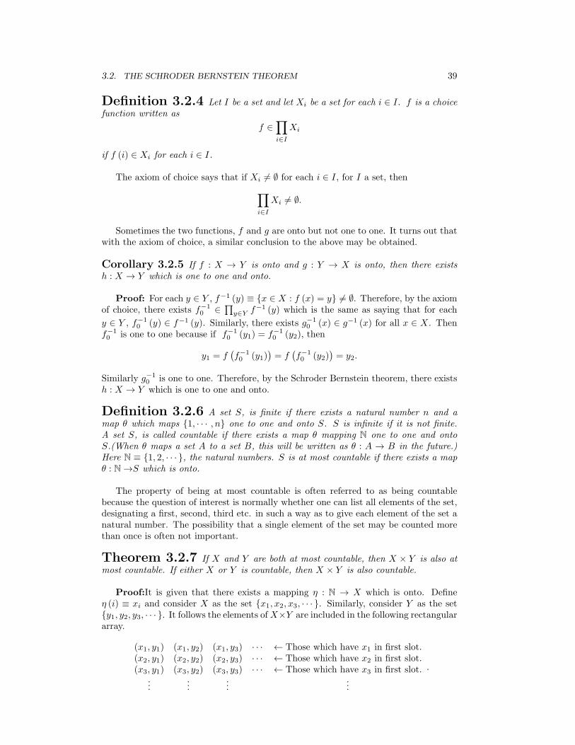
3.2. THE SCHRODER BERNSTEIN THEOREM 39
Definition 3.2.4 Let I be a set and let Xi be a set for each i ∈ I. f is a choicefunction written as
f ∈∏i∈I
Xi
if f (i) ∈ Xi for each i ∈ I.
The axiom of choice says that if Xi = ∅ for each i ∈ I, for I a set, then∏i∈I
Xi = ∅.
Sometimes the two functions, f and g are onto but not one to one. It turns out thatwith the axiom of choice, a similar conclusion to the above may be obtained.
Corollary 3.2.5 If f : X → Y is onto and g : Y → X is onto, then there existsh : X → Y which is one to one and onto.
Proof: For each y ∈ Y , f−1 (y) ≡ {x ∈ X : f (x) = y} = ∅. Therefore, by the axiomof choice, there exists f−1
0 ∈∏
y∈Y f−1 (y) which is the same as saying that for each
y ∈ Y , f−10 (y) ∈ f−1 (y). Similarly, there exists g−1
0 (x) ∈ g−1 (x) for all x ∈ X. Thenf−10 is one to one because if f−1
0 (y1) = f−10 (y2), then
y1 = f(f−10 (y1)
)= f
(f−10 (y2)
)= y2.
Similarly g−10 is one to one. Therefore, by the Schroder Bernstein theorem, there exists
h : X → Y which is one to one and onto.
Definition 3.2.6 A set S, is finite if there exists a natural number n and amap θ which maps {1, · · · , n} one to one and onto S. S is infinite if it is not finite.A set S, is called countable if there exists a map θ mapping N one to one and ontoS.(When θ maps a set A to a set B, this will be written as θ : A → B in the future.)Here N ≡ {1, 2, · · · }, the natural numbers. S is at most countable if there exists a mapθ : N→S which is onto.
The property of being at most countable is often referred to as being countablebecause the question of interest is normally whether one can list all elements of the set,designating a first, second, third etc. in such a way as to give each element of the set anatural number. The possibility that a single element of the set may be counted morethan once is often not important.
Theorem 3.2.7 If X and Y are both at most countable, then X × Y is also atmost countable. If either X or Y is countable, then X × Y is also countable.
Proof:It is given that there exists a mapping η : N → X which is onto. Defineη (i) ≡ xi and consider X as the set {x1, x2, x3, · · · }. Similarly, consider Y as the set{y1, y2, y3, · · · }. It follows the elements ofX×Y are included in the following rectangulararray.
(x1, y1) (x1, y2) (x1, y3) · · · ← Those which have x1 in first slot.(x2, y1) (x2, y2) (x2, y3) · · · ← Those which have x2 in first slot.(x3, y1) (x3, y2) (x3, y3) · · · ← Those which have x3 in first slot.
......
......
.
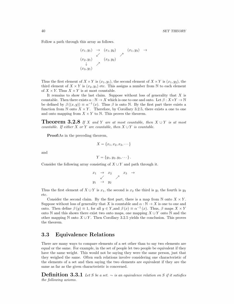
40 SET THEORY
Follow a path through this array as follows.
(x1, y1) → (x1, y2) (x1, y3) →↙ ↗
(x2, y1) (x2, y2)↓ ↗
(x3, y1)
Thus the first element of X × Y is (x1, y1), the second element of X × Y is (x1, y2), thethird element of X × Y is (x2, y1) etc. This assigns a number from N to each elementof X × Y. Thus X × Y is at most countable.
It remains to show the last claim. Suppose without loss of generality that X iscountable. Then there exists α : N→ X which is one to one and onto. Let β : X×Y → Nbe defined by β ((x, y)) ≡ α−1 (x). Thus β is onto N. By the first part there exists afunction from N onto X × Y . Therefore, by Corollary 3.2.5, there exists a one to oneand onto mapping from X × Y to N. This proves the theorem.
Theorem 3.2.8 If X and Y are at most countable, then X ∪ Y is at mostcountable. If either X or Y are countable, then X ∪ Y is countable.
Proof:As in the preceding theorem,
X = {x1, x2, x3, · · · }
andY = {y1, y2, y3, · · · } .
Consider the following array consisting of X ∪ Y and path through it.
x1 → x2 x3 →↙ ↗
y1 → y2
Thus the first element of X ∪ Y is x1, the second is x2 the third is y1 the fourth is y2etc.
Consider the second claim. By the first part, there is a map from N onto X × Y .Suppose without loss of generality that X is countable and α : N→ X is one to one andonto. Then define β (y) ≡ 1, for all y ∈ Y ,and β (x) ≡ α−1 (x). Thus, β maps X × Yonto N and this shows there exist two onto maps, one mapping X ∪ Y onto N and theother mapping N onto X ∪ Y . Then Corollary 3.2.5 yields the conclusion. This provesthe theorem.
3.3 Equivalence Relations
There are many ways to compare elements of a set other than to say two elements areequal or the same. For example, in the set of people let two people be equivalent if theyhave the same weight. This would not be saying they were the same person, just thatthey weighed the same. Often such relations involve considering one characteristic ofthe elements of a set and then saying the two elements are equivalent if they are thesame as far as the given characteristic is concerned.
Definition 3.3.1 Let S be a set. ∼ is an equivalence relation on S if it satisfiesthe following axioms.

3.4. EXERCISES 41
1. x ∼ x for all x ∈ S. (Reflexive)
2. If x ∼ y then y ∼ x. (Symmetric)
3. If x ∼ y and y ∼ z, then x ∼ z. (Transitive)
Definition 3.3.2 [x] denotes the set of all elements of S which are equivalentto x and [x] is called the equivalence class determined by x or just the equivalence classof x.
With the above definition one can prove the following simple theorem.
Theorem 3.3.3 Let ∼ be an equivalence class defined on a set, S and let Hdenote the set of equivalence classes. Then if [x] and [y] are two of these equivalenceclasses, either x ∼ y and [x] = [y] or it is not true that x ∼ y and [x] ∩ [y] = ∅.
3.4 Exercises
1. The Barber of Seville is a man and he shaves exactly those men who do not shavethemselves. Who shaves the Barber?
2. Do you believe each person who has ever lived on this earth has the right to dowhatever he or she wants? (Note the use of the universal quantifier with no set insight.) If you believe this, do you really believe what you say you believe? Whatof those people who want to deprive others their right to do what they want? Dopeople often use quantifiers this way?
3. President Bush, when he found there were no weapons of mass destruction saidwe would give the Iraqi’s “freedom”. He is protecting our “freedom”. Whatis freedom? Is there an implied quantifier involved? Is there a set mentioned?What is the meaning of the statement? Could it mean different things to differentpeople?
4. DeMorgan’s laws are very useful in mathematics. Let S be a set of sets each ofwhich is contained in some universal set, U . Show
∪{AC : A ∈ S
}= (∩{A : A ∈ S})C
and
∩{AC : A ∈ S
}= (∪{A : A ∈ S})C .
5. Let S be a set of sets show
B ∪ ∪{A : A ∈ S} = ∪{B ∪A : A ∈ S} .
6. Let S be a set of sets show
B ∩ ∪{A : A ∈ S} = ∪{B ∩A : A ∈ S} .
7. Show the rational numbers are countable, this is in spite of the fact that betweenany two integers there are infinitely many rational numbers. What does this showabout the usefulness of common sense and instinct in mathematics?

42 SET THEORY
8. We say a number is an algebraic number if it is the solution of an equation of theform
anxn + · · ·+ a1x+ a0 = 0
where all the aj are integers and all exponents are also integers. Thus√2 is an
algebraic number because it is a solution of the equation x2 − 2 = 0. Using theobservation that any such equation has at most n solutions, show the set of allalgebraic numbers is countable.
9. Let A be a nonempty set and let P (A) be its power set, the set of all subsets ofA. Show there does not exist any function f , which maps A onto P (A). Thusthe power set is always strictly larger than the set from which it came. Hint:Suppose f is onto. Consider S ≡ {x ∈ A : x /∈ f (x)}. If f is onto, then f (y) = Sfor some y ∈ A. Is y ∈ f (y)? Note this argument holds for sets of any size.
10. The empty set is said to be a subset of every set. Why? Consider the statement:If pigs had wings, then they could fly. Is this statement true or false?
11. If S = {1, · · · , n}, show P (S) has exactly 2n elements in it. Hint: You might trya few cases first.
12. Show the set of all subsets of N, the natural numbers, which have 3 elements,is countable. Is the set of all subsets of N which have finitely many elementscountable? How about the set of all subsets of N?
13. Prove Theorem 3.3.3.
14. Let S be a set and consider a function f which maps P (S) to P (S) which satisfiesthe following. If A ⊆ B, then f (A) ⊆ f (B). Show there exists A such thatf (A) = A. Hint: You might consider the following subset of P (S) .
C ≡ {B ∈ P (S) : B ⊆ f (B)}
Then consider A ≡ ∪C. Argue A is the “largest” set in C which implies A cannotbe a proper subset of f (A).

Functions And Sequences
4.1 General Considerations
The concept of a function is that of something which gives a unique output for a giveninput.
Definition 4.1.1 Consider two sets, D and R along with a rule which assignsa unique element of R to every element of D. This rule is called a function and it isdenoted by a letter such as f. The symbol, D (f) = D is called the domain of f. Theset R, also written R (f) , is called the range of f. The set of all elements of R whichare of the form f (x) for some x ∈ D is often denoted by f (D) . When R = f (D), thefunction f , is said to be onto. It is common notation to write f : D (f)→ R to denotethe situation just described in this definition where f is a function defined on D havingvalues in R.
Example 4.1.2 Consider the list of numbers, {1, 2, 3, 4, 5, 6, 7} ≡ D. Define a functionwhich assigns an element of D to R ≡ {2, 3, 4, 5, 6, 7, 8} by f (x) ≡ x+1 for each x ∈ D.
In this example there was a clearly defined procedure which determined the function.However, sometimes there is no discernible procedure which yields a particular function.
Example 4.1.3 Consider the ordered pairs, (1, 2) , (2,−2) , (8, 3) , (7, 6) and let
D ≡ {1, 2, 8, 7} ,
the set of first entries in the given set of ordered pairs, R ≡ {2,−2, 3, 6} , the set ofsecond entries, and let f (1) = 2, f (2) = −2, f (8) = 3, and f (7) = 6.
Sometimes functions are not given in terms of a formula. For example, consider thefollowing function defined on the positive real numbers having the following definition.
Example 4.1.4 For x ∈ R define
f (x) =
{1n if x = m
n in lowest terms for m,n ∈ Z0 if x is not rational
(4.1)
This is a very interesting function called the Dirichlet function. Note that it is notdefined in a simple way from a formula.
Example 4.1.5 Let D consist of the set of people who have lived on the earth exceptfor Adam and for d ∈ D, let f (d) ≡ the biological father of d. Then f is a function.
43
44 FUNCTIONS AND SEQUENCES
This function is not the sort of thing studied in calculus but it is a function just thesame. When D (f) is not specified, it is understood to consist of everything for whichf makes sense. The following definition gives several ways to make new functions fromold ones.
Definition 4.1.6 Let f, g be functions with values in F. Let a, b be points of F.Then af + bg is the name of a function whose domain is D (f)∩D (g) which is definedas
(af + bg) (x) = af (x) + bg (x) .
The function fg is the name of a function which is defined on D (f) ∩D (g) given by
(fg) (x) = f (x) g (x) .
Similarly for k an integer, fk is the name of a function defined as
fk (x) = (f (x))k
The function f/g is the name of a function whose domain is
D (f) ∩ {x ∈ D (g) : g (x) = 0}
defined as(f/g) (x) = f (x) /g (x) .
If f : D (f)→ X and g : D (g)→ Y, then g ◦ f is the name of a function whose domainis
{x ∈ D (f) : f (x) ∈ D (g)}
which is defined asg ◦ f (x) ≡ g (f (x)) .
This is called the composition of the two functions.
You should note that f (x) is not a function. It is the value of the function at thepoint, x. The name of the function is f. Nevertheless, people often write f (x) to denotea function and it doesn’t cause too many problems in beginning courses. When this isdone, the variable, x should be considered as a generic variable free to be anything inD (f) .
Sometimes people get hung up on formulas and think that the only functions ofimportance are those which are given by some simple formula. It is a mistake to thinkthis way. Functions involve a domain and a range and a function is determined by whatit does.
Example 4.1.7 Let f (t) = t and g (t) = 1 + t. Then fg : R→ R is given by
fg (t) = t (1 + t) = t+ t2.
Example 4.1.8 Let f (t) = 2t+ 1 and g (t) =√1 + t. Then
g ◦ f (t) =√1 + (2t+ 1) =
√2t+ 2
for t ≥ −1. If t < −1 the inside of the square root sign is negative so makes no sense.Therefore, g ◦ f : {t ∈ R : t ≥ −1} → R.
Note that in this last example, it was necessary to fuss about the domain of g ◦ fbecause g is only defined for certain values of t.
The concept of a one to one function is very important. This is discussed in thefollowing definition.

4.1. GENERAL CONSIDERATIONS 45
Definition 4.1.9 For any function f : D (f) ⊆ X → Y, define the following setknown as the inverse image of y.
f−1 (y) ≡ {x ∈ D (f) : f (x) = y} .
There may be many elements in this set, but when there is always only one element inthis set for all y ∈ f (D (f)) , the function f is one to one sometimes written, 1 − 1.Thus f is one to one, 1 − 1, if whenever f (x) = f (x1) , then x = x1. If f is one toone, the inverse function f−1 is defined on f (D (f)) and f−1 (y) = x where f (x) = y.Thus from the definition, f−1 (f (x)) = x for all x ∈ D (f) and f
(f−1 (y)
)= y for all
y ∈ f (D (f)) . Defining id by id (z) ≡ z this says f ◦ f−1 = id and f−1 ◦ f = id .
Polynomials and rational functions are particularly easy functions to understandbecause they do come from a simple formula.
Definition 4.1.10 A function f is a polynomial if
f (x) = anxn + an−1x
n−1 + · · ·+ a1x+ a0
where the ai are real or complex numbers and n is a nonnegative integer. In this casethe degree of the polynomial, f (x) is n. Thus the degree of a polynomial is the largestexponent appearing on the variable.
f is a rational function if
f (x) =h (x)
g (x)
where h and g are polynomials.
For example, f (x) = 3x5 + 9x2 + 7x+ 5 is a polynomial of degree 5 and
3x5 + 9x2 + 7x+ 5
x4 + 3x+ x+ 1
is a rational function.Note that in the case of a rational function, the domain of the function might not
be all of F. For example, if
f (x) =x2 + 8
x+ 1,
the domain of f would be all complex numbers not equal to −1.Closely related to the definition of a function is the concept of the graph of a function.
Definition 4.1.11 Given two sets, X and Y, the Cartesian product of the twosets, written as X × Y, is assumed to be a set described as follows.
X × Y = {(x, y) : x ∈ X and y ∈ Y } .
F2 denotes the Cartesian product of F with F. Recall F could be either R or C.
The notion of Cartesian product is just an abstraction of the concept of identifyinga point in the plane with an ordered pair of numbers.
Definition 4.1.12 Let f : D (f)→ R (f) be a function. The graph of f consistsof the set,
{(x, y) : y = f (x) for x ∈ D (f)} .
Note that knowledge of the graph of a function is equivalent to knowledge of thefunction. To find f (x) , simply observe the ordered pair which has x as its first elementand the value of y equals f (x) .
46 FUNCTIONS AND SEQUENCES
4.2 Sequences
Functions defined on the set of integers larger than a given integer are called sequences.
Definition 4.2.1 A function whose domain is defined as a set of the form
{k, k + 1, k + 2, · · · }
for k an integer is known as a sequence. Thus you can consider f (k) , f (k + 1) , f (k + 2) ,etc. Usually the domain of the sequence is either N, the natural numbers consisting of{1, 2, 3, · · · } or the nonnegative integers, {0, 1, 2, 3, · · · } . Also, it is traditional to writef1, f2, etc. instead of f (1) , f (2) , f (3) etc. when referring to sequences. In the abovecontext, fk is called the first term, fk+1 the second and so forth. It is also common towrite the sequence, not as f but as {fi}∞i=k or just {fi} for short.
Example 4.2.2 Let {ak}∞k=1 be defined by ak ≡ k2 + 1.
This gives a sequence. In fact, a7 = a (7) = 72 + 1 = 50 just from using the formulafor the kth term of the sequence.
It is nice when sequences come in this way from a formula for the kth term. However,this is often not the case. Sometimes sequences are defined recursively. This happens,when the first several terms of the sequence are given and then a rule is specified whichdetermines an+1 from knowledge of a1, · · · , an. This rule which specifies an+1 fromknowledge of ak for k ≤ n is known as a recurrence relation.
Example 4.2.3 Let a1 = 1 and a2 = 1. Assuming a1, · · · , an+1 are known, an+2 ≡an + an+1.
Thus the first several terms of this sequence, listed in order, are 1, 1, 2, 3, 5, 8,· · · .This particular sequence is called the Fibonacci sequence and is important in the studyof reproducing rabbits. Note this defines a function without giving a formula for it.Such sequences occur naturally in the solution of differential equations using powerseries methods and in many other situations of great importance.
For sequences, it is very important to consider something called a subsequence.
Definition 4.2.4 Let {an} be a sequence and let n1 < n2 < n3, · · · be anystrictly increasing list of integers such that n1 is at least as large as the first number inthe domain of the function. Then if bk ≡ ank
, {bk} is called a subsequence of {an} .
For example, suppose an =(n2 + 1
). Thus a1 = 2, a3 = 10, etc. If
n1 = 1, n2 = 3, n3 = 5, · · · , nk = 2k − 1,
then letting bk = ank, it follows
bk =((2k − 1)
2+ 1)= 4k2 − 4k + 2.
4.3 Exercises
1. Let g (t) ≡√2− t and let f (t) = 1
t . Find g ◦ f. Include the domain of g ◦ f. Youcan believe for now that the square root of any positive number exists. This willbe shown later.
2. Give the domains of the following functions.

4.3. EXERCISES 47
(a) f (x) = x+33x−2
(b) f (x) =√x2 − 4
(c) f (x) =√4− x2
(d) f (x) =√
x 43x+5
(e) f (x) =√
x2−4x+1
3. Let f : R→ R be defined by f (t) ≡ t3 + 1. Is f one to one? Can you find aformula for f−1?
4. Suppose a1 = 1, a2 = 3, and a3 = −1. Suppose also that for n ≥ 4 it is knownthat an = an−1+2an−2+3an−3. Find a7. Are you able to guess a formula for thekth term of this sequence?
5. Let f : {t ∈ R : t = −1}→ R be defined by f (t) ≡ tt+1 . Find f
−1 if possible.
6. A function f : R→ R is a strictly increasing function if whenever x < y, it followsthat f (x) < f (y) . If f is a strictly increasing function, does f−1 always exist?Explain your answer.
7. Let f (t) be defined by
f (t) =
{2t+ 1 if t ≤ 1t if t > 1
.
Find f−1 if possible.
8. Suppose f : D (f)→ R (f) is one to one, R (f) ⊆ D (g) , and g : D (g)→ R (g) isone to one. Does it follow that g ◦ f is one to one?
9. If f : R→ R and g : R→ R are two one to one functions, which of the followingare necessarily one to one on their domains? Explain why or why not by giving aproof or an example.
(a) f + g
(b) fg
(c) f3
(d) f/g
10. Draw the graph of the function f (x) = x3 + 1.
11. Draw the graph of the function f (x) = x2 + 2x+ 2.
12. Draw the graph of the function f (x) = x1+x .
13. Suppose an = 1n and let nk = 2k. Find bk where bk = ank
.
14. If Xi are sets and for some j, Xj = ∅, the empty set. Verify carefully that∏ni=1Xi = ∅.
15. Suppose f (x) + f(1x
)= 7x and f is a function defined on R\ {0} , the nonzero
real numbers. Find all values of x where f (x) = 1 if there are any. Does thereexist any such function?
16. Does there exist a function f , satisfying f (x)− f(1x
)= 3x which has both x and
1x in the domain of f?
48 FUNCTIONS AND SEQUENCES
17. In the situation of the Fibonacci sequence show that the formula for the nth termcan be found and is given by
an =
√5
5
(1 +√5
2
)n
−√5
5
(1−√5
2
)n
.
Hint: You might be able to do this by induction but a better way would be tolook for a solution to the recurrence relation, an+2 ≡ an + an+1 of the form rn.You will be able to show that there are two values of r which work, one of which
is r = 1+√5
2 . Next you can observe that if rn1 and rn2 both satisfy the recurrencerelation then so does crn1 + drn2 for any choice of constants c, d. Then you try topick c and d such that the conditions, a1 = 1 and a2 = 1 both hold.
18. In an ordinary annuity, you make constant payments, P at the beginning of eachpayment period. These accrue interest at the rate of r per payment period. Thismeans at the start of the first payment period, there is the payment P ≡ A1. Thenthis produces an amount rP in interest so at the beginning of the second paymentperiod, you would have rP + P + P ≡ A2. Thus A2 = A1 (1 + r) + P. Then atthe beginning of the third payment period you would have A2 (1 + r) + P ≡ A3.Continuing in this way, you see that the amount in at the beginning of the nth
payment period would be An given by An = An−1 (1 + r) + P and A1 = P. ThusA is a function defined on the positive integers given recursively as just describedand An is the amount at the beginning of the nth payment period. Now if youwanted to find out An for large n, how would you do it? One way would be to usethe recurrance relation n times. A better way would be to find a formula for An.Look for one in the form An = Czn + s where C, z and s are to be determined.Show that C = P
r , z = (1 + r) , and s = −Pr .
19. A well known puzzle consists of three pegs and several disks each of a differentdiameter, each having a hole in the center which allows it to be slid down eachof the pegs. These disks are piled one on top of the other on one of the pegs,in order of decreasing diameter, the larger disks always being below the smallerdisks. The problem is to move the whole pile of disks to another peg such thatyou never place a disk on a smaller disk. If you have n disks, how many moveswill it take? Of course this depends on n. If n = 1, you can do it in one move. Ifn = 2, you would need 3. Let An be the number required for n disks. Then insolving the puzzle, you must first obtain the top n− 1 disks arranged in order onanother peg before you can move the bottom disk of the original pile. This takesAn−1 moves. Explain why An = 2An−1 + 1, A1 = 1 and give a formula for An.Look for one in the form An = Crn + s. This puzzle is called the Tower of Hanoi.When you have found a formula for An, explain why it is not possible to do thispuzzle if n is very large.
4.4 Worked Exercises
1. Suppose f (x) + f(1x
)= 7x and f is a function defined on R\ {0} , the nonzero
real numbers. Find all values of x where f (x) = 1 if there are any. Does thereexist any such function?
The existence of such a function is problematic. If you assume it exists, you couldreplace x with 1/y and then conclude f (y) + f (1/y) = 7/y. Now this would holdfor all y = 0. Hence you would need to have 7x = 7/x and so x = ±1.
4.4. WORKED EXERCISES 49
2. In the situation of the Fibonacci sequence show that the formula for the nth termcan be found and is given by
an =
√5
5
(1 +√5
2
)n
−√5
5
(1−√5
2
)n
.
Hint: You might be able to do this by induction but a better way would be tolook for a solution to the recurrence relation, an+2 ≡ an + an+1 of the form rn.You will be able to show that there are two values of r which work, one of which
is r = 1+√5
2 . Next you can observe that if rn1 and rn2 both satisfy the recurrencerelation then so does crn1 + drn2 for any choice of constants c, d. Then you try topick c and d such that the conditions, a1 = 1 and a2 = 1 both hold.
Look for a solution of the for described above. Then you would need
rn+2 = rn+1 + rn
and so r2 = r + 1, Solution is :{r = 1
2
√5 + 1
2
},{r = 1
2 −12
√5}. Now note that
anything if rn1 works and rn2 also satisfies the recurrence relation, then so doesC1r
n1 + C2r
n2 . Hence anything of the form
C1
(1
2
√5 +
1
2
)n
+ C2
(1
2− 1
2
√5
)n
will work. You just need to satisfy the initial conditions. Letting n = 1 and n = 2you want to get 1. thus you need
C1
(12
√5 + 1
2
)+ C2
(12 −
12
√5)= 1
C1
(12
√5 + 1
2
)2+ C2
(12 −
12
√5)2
= 1
You solve these equations. Solution is :{C2 = − 1
5
√5, C1 = 1
5
√5}. Therefore,
you need
an =1
5
√5
(1
2
√5 +
1
2
)n
− 1
5
√5
(1
2− 1
2
√5
)n
3. In an ordinary annuity, you make constant payments, P at the beginning of eachpayment period. These accrue interest at the rate of r per payment period. Thismeans at the start of the first payment period, there is the payment P ≡ A1. Thenthis produces an amount rP in interest so at the beginning of the second paymentperiod, you would have rP + P + P ≡ A2. Thus A2 = A1 (1 + r) + P. Then atthe beginning of the third payment period you would have A2 (1 + r) + P ≡ A3.Continuing in this way, you see that the amount in at the beginning of the nth
payment period would be An given by An = An−1 (1 + r) + P and A1 = P. ThusA is a function defined on the positive integers given recursively as just describedand An is the amount at the beginning of the nth payment period. Now if youwanted to find out An for large n, how would you do it? One way would be to usethe recurrance relation n times. A better way would be to find a formula for An.Look for one in the form An = Czn + s where C, z and s are to be determined.Show that C = P
r , z = (1 + r) , and s = −Pr .
An = An−1 (1 + r) + P and we use the suggestion. Then
Czn + s =(Czn−1 + s
)(1 + r) + P
ThusC(zn − (1 + r) zn−1
)= sr + P
50 FUNCTIONS AND SEQUENCES
As n changes, the left side changes also but the right side doesn’t change. Thusyou need z = (1 + r). Hence you also need to have s = −P/r. Thus the formulafor the annuity is
An = C (1 + r)n − P/r
and you want A1 = P and so
C (1 + r)− P/r = P
which requires C = Pr . Then
An =P
r((1 + r)
n − 1) .
4. A well known puzzle consists of three pegs and several disks each of a differentdiameter, each having a hole in the center which allows it to be slid down eachof the pegs. These disks are piled one on top of the other on one of the pegs,in order of decreasing diameter, the larger disks always being below the smallerdisks. The problem is to move the whole pile of disks to another peg such thatyou never place a disk on a smaller disk. If you have n disks, how many moveswill it take? Of course this depends on n. If n = 1, you can do it in one move. Ifn = 2, you would need 3. Let An be the number required for n disks. Then insolving the puzzle, you must first obtain the top n− 1 disks arranged in order onanother peg before you can move the bottom disk of the original pile. This takesAn−1 moves. Explain why An = 2An−1 + 1, A1 = 1 and give a formula for An.Look for one in the form An = Crn + s. This puzzle is called the Tower of Hanoi.When you have found a formula for An, explain why it is not possible to do thispuzzle if n is very large.
You do it the same as before.
Crn + s = 2(Crn−1 + s
)+ 1
Then taking the stuff with r to one side, it follows you must have
r = 2
and then you just need to find C. When n = 1 you are supposed to get 1. Whenn = 2 you need 3= A2. Thus you need
1 = C2 + s, 3 = C4 + s
Thus s = −1 and C = 1. Hence An = 2n − 1.
4.5 The Limit Of A Sequence
The concept of the limit of a sequence was defined precisely by Bolzano.1 The followingis the precise definition of what is meant by the limit of a sequence.
1Bernhard Bolzano lived from 1781 to 1848. He was a Catholic priest and held a position inphilosophy at the University of Prague. He had strong views about the absurdity of war, educationalreform, and the need for individual concience. His convictions got him in trouble with Emporer FranzI of Austria and when he refused to recant, was forced out of the university. He understood the needfor absolute rigor in mathematics. He also did work on physics.
4.5. THE LIMIT OF A SEQUENCE 51
Definition 4.5.1 A sequence {an}∞n=1 converges to a,
limn→∞
an = a or an → a
if and only if for every ε > 0 there exists nε such that whenever n ≥ nε ,
|an − a| < ε.
Here a and an are assumed to be complex numbers but the same definition holds moregenerally.
In words the definition says that given any measure of closeness, ε, the terms of thesequence are eventually this close to a. Here, the word “eventually” refers to n beingsufficiently large. The above definition is always the definition of what is meant by thelimit of a sequence. If the an are complex numbers or later on, vectors the definition
remains the same. If an = xn + iyn and a = x+ iy, |an − a| =√
(xn − x)2 + (yn − y)2.Recall the way you measure distance between two complex numbers.
Theorem 4.5.2 If limn→∞ an = a and limn→∞ an = a1 then a1 = a.
Proof:Suppose a1 = a. Then let 0 < ε < |a1 − a| /2 in the definition of the limit.It follows there exists nε such that if n ≥ nε, then |an − a| < ε and |an − a1| < ε.Therefore, for such n,
|a1 − a| ≤ |a1 − an|+ |an − a|< ε+ ε < |a1 − a| /2 + |a1 − a| /2 = |a1 − a| ,
a contradiction.
Example 4.5.3 Let an = 1n2+1 .
Then it seems clear that
limn→∞
1
n2 + 1= 0.
In fact, this is true from the definition. Let ε > 0 be given. Let nε ≥√ε−1. Then if
n > nε ≥√ε−1,
it follows that n2 + 1 > ε−1 and so
0 <1
n2 + 1= an < ε..
Thus |an − 0| < ε whenever n is this large.Note the definition was of no use in finding a candidate for the limit. This had to
be produced based on other considerations. The definition is for verifying beyond anydoubt that something is the limit. It is also what must be referred to in establishingtheorems which are good for finding limits.
Example 4.5.4 Let an = n2
Then in this case limn→∞ an does not exist.
Example 4.5.5 Let an = (−1)n .

52 FUNCTIONS AND SEQUENCES
In this case, limn→∞ (−1)n does not exist. This follows from the definition. Letε = 1/2. If there exists a limit, l, then eventually, for all n large enough, |an − l| < 1/2.However, |an − an+1| = 2 and so,
2 = |an − an+1| ≤ |an − l|+ |l − an+1| < 1/2 + 1/2 = 1
which cannot hold. Therefore, there can be no limit for this sequence.
Theorem 4.5.6 Suppose {an} and {bn} are sequences and that
limn→∞
an = a and limn→∞
bn = b.
Also suppose x and y are in F. Then
limn→∞
xan + ybn = xa+ yb (4.2)
limn→∞
anbn = ab (4.3)
If b = 0,
limn→∞
anbn
=a
b. (4.4)
Proof: The first of these claims is left for you to do. To do the second, let ε > 0 begiven and choose n1 such that if n ≥ n1 then
|an − a| < 1.
Then for such n, the triangle inequality implies
|anbn − ab| ≤ |anbn − anb|+ |anb− ab|≤ |an| |bn − b|+ |b| |an − a|≤ (|a|+ 1) |bn − b|+ |b| |an − a| .
Now let n2 be large enough that for n ≥ n2,
|bn − b| <ε
2 (|a|+ 1), and |an − a| <
ε
2 (|b|+ 1).
Such a number exists because of the definition of limit. Therefore, let
nε > max (n1, n2) .
For n ≥ nε,
|anbn − ab| ≤ (|a|+ 1) |bn − b|+ |b| |an − a|
< (|a|+ 1)ε
2 (|a|+ 1)+ |b| ε
2 (|b|+ 1)≤ ε.
This proves 4.3. Next consider 4.4.Let ε > 0 be given and let n1 be so large that whenever n ≥ n1,
|bn − b| <|b|2.
Thus for such n,∣∣∣∣anbn − a
b
∣∣∣∣ = ∣∣∣∣anb− abnbbn
∣∣∣∣ ≤ 2
|b|2[|anb− ab|+ |ab− abn|]

4.5. THE LIMIT OF A SEQUENCE 53
≤ 2
|b||an − a|+
2 |a||b|2|bn − b| .
Now choose n2 so large that if n ≥ n2, then
|an − a| <ε |b|4, and |bn − b| <
ε |b|2
4 (|a|+ 1).
Letting nε > max (n1, n2) , it follows that for n ≥ nε,∣∣∣∣anbn − a
b
∣∣∣∣ ≤ 2
|b||an − a|+
2 |a||b|2|bn − b|
<2
|b|ε |b|4
+2 |a||b|2
ε |b|2
4 (|a|+ 1)< ε.
Another very useful theorem for finding limits is the squeezing theorem.
Theorem 4.5.7 Suppose limn→∞ an = a = limn→∞ bn and an ≤ cn ≤ bn forall n large enough. Then limn→∞ cn = a.
Proof: Let ε > 0 be given and let n1 be large enough that if n ≥ n1,
|an − a| < ε/2 and |bn − a| < ε/2.
Then for such n,|cn − a| ≤ |an − a|+ |bn − a| < ε.
The reason for this is that if cn ≥ a, then
|cn − a| = cn − a ≤ bn − a ≤ |an − a|+ |bn − a|
because bn ≥ cn. On the other hand, if cn ≤ a, then
|cn − a| = a− cn ≤ a− an ≤ |a− an|+ |b− bn| .
This proves the theorem.As an example, consider the following.
Example 4.5.8 Let
cn ≡ (−1)n 1
n
and let bn = 1n , and an = − 1
n . Then you may easily show that
limn→∞
an = limn→∞
bn = 0.
Since an ≤ cn ≤ bn, it follows limn→∞ cn = 0 also.
Theorem 4.5.9 limn→∞ rn = 0. Whenever |r| < 1.
Proof:If 0 < r < 1 if follows r−1 > 1. Why? Letting α = 1r − 1, it follows
r =1
1 + α.
Therefore, by the binomial theorem,
0 < rn =1
(1 + α)n ≤
1
1 + αn.
Therefore, limn→∞ rn = 0 if 0 < r < 1. Now in general, if |r| < 1, |rn| = |r|n → 0 bythe first part. This proves the theorem.
An important theorem is the one which states that if a sequence converges, so doesevery subsequence. You should review Definition 4.2.4 on Page 46 at this point.

54 FUNCTIONS AND SEQUENCES
Theorem 4.5.10 Let {xn} be a sequence with limn→∞ xn = x and let {xnk} be
a subsequence. Then limk→∞ xnk= x.
Proof:Let ε > 0 be given. Then there exists nε such that if n > nε, then |xn − x| <ε. Suppose k > nε. Then nk ≥ k > nε and so
|xnk− x| < ε
showing limk→∞ xnk= x as claimed.
Theorem 4.5.11 Let {xn} be a sequence of real numbers and suppose eachxn ≤ l (≥ l)and limn→∞ xn = x. Then x ≤ l (≥ l) . More generally, suppose {xn}and {yn} are two sequences such that limn→∞ xn = x and limn→∞ yn = y. Then ifxn ≤ yn for all n sufficiently large, then x ≤ y.
Proof: Let ε > 0 be given. Then for n large enough,
l ≥ xn > x− ε
and sol + ε ≥ x.
Since ε > 0 is arbitrary, this requires l ≥ x. The other case is entirely similar or elseyou could consider −l and {−xn} and apply the case just considered.
Consider the last claim. There exists N such that if n ≥ N then xn ≤ yn and
|x− xn|+ |y − yn| < ε/2.
Then considering n > N in what follows, the above implies that
x < xn + ε/2, and y > yn − ε/2.
Therefore,x− y ≤ xn + ε/2− (yn − ε/2) = xn − yn + ε ≤ ε.
Since ε was arbitrary, it followsx− y ≤ 0.
This proves the theorem.
4.6 The Nested Interval Lemma
In Russia there is a kind of doll called a matrushka doll. You pick it up and notice itcomes apart in the center. Separating the two halves you find an identical doll inside.Then you notice this inside doll also comes apart in the center. Separating the twohalves, you find yet another identical doll inside. This goes on quite a while until thefinal doll is in one piece. The nested interval lemma is like a matrushka doll exceptthe process never stops. It involves a sequence of intervals, the first containing thesecond, the second containing the third, the third containing the fourth and so on. Thefundamental question is whether there exists a point in all the intervals. Sometimesthere is such a point and this comes from completeness.
Lemma 4.6.1 Let Ik =[ak, bk
]and suppose that for all k = 1, 2, · · · ,
Ik ⊇ Ik+1.
Then there exists a point, c ∈ R which is an element of every Ik.
4.7. EXERCISES 55
Proof:Since Ik ⊇ Ik+1, this implies
ak ≤ ak+1, bk ≥ bk+1. (4.5)
Consequently, if k ≤ l,al ≤ al ≤ bl ≤ bk. (4.6)
Now definec ≡ sup
{al : l = 1, 2, · · ·
}By the first inequality in 4.5, and 4.6
ak ≤ c = sup{al : l = k, k + 1, · · ·
}≤ bk (4.7)
for each k = 1, 2 · · · . Thus c ∈ Ik for every k and this proves the lemma. If this wenttoo fast, the reason for the last inequality in 4.7 is that from 4.6, bk is an upper boundto{al : l = k, k + 1, · · ·
}. Therefore, it is at least as large as the least upper bound.
This is really quite a remarkable result and may not seem so obvious. Consider theintervals Ik ≡ (0, 1/k) . Then there is no point which lies in all these intervals becauseno negative number can be in all the intervals and 1/k is smaller than a given positivenumber whenever k is large enough. Thus the only candidate for being in all the intervalsis 0 and 0 has been left out of them all. The problem here is that the endpoints of theintervals were not included, contrary to the hypotheses of the above lemma in which allthe intervals included the endpoints.
4.7 Exercises
1. Find limn→∞n
3n+4 .
2. Find limn→∞3n4+7n+1000
n4+1 .
3. Find limn→∞2n+7(5n)4n+2(5n) .
4. Find limn→∞√
(n2 + 6n)− n. Hint: Multiply and divide by√(n2 + 6n) + n.
5. Find limn→∞∑n
k=11
10k.
6. Suppose {xn + iyn} is a sequence of complex numbers which converges to thecomplex number x+ iy. Show this happens if and only if xn → x and yn → y.
7. For |r| < 1, find limn→∞∑n
k=0 rk. Hint: First show
∑nk=0 r
k = rn+1
r−1 −1
r−1 . Thenrecall Theorem 4.5.9.
8. Using the binomial theorem prove that for all n ∈ N,(1 + 1
n
)n ≤ (1 + 1n+1
)n+1
.
Hint: Show first that(nk
)= n·(n−1)···(n−k+1)
k! . By the binomial theorem,
(1 +
1
n
)n
=n∑
k=0
(n
k
)(1
n
)k
=n∑
k=0
k factors︷ ︸︸ ︷n · (n− 1) · · · (n− k + 1)
k!nk.
Now consider the term n·(n−1)···(n−k+1)k!nk and note that a similar term occurs in the
binomial expansion for(1 + 1
n+1
)n+1
except you replace n with n+ 1 whereever
this occurs. Argue the term got bigger and then note that in the binomial expan-
sion for(1 + 1
n+1
)n+1
, there are more terms.

56 FUNCTIONS AND SEQUENCES
9. Prove by induction that for all k ≥ 4, 2k ≤ k!
10. Use the Problems 21 and 8 to verify for all n ∈ N,(1 + 1
n
)n ≤ 3.
11. Prove limn→∞(1 + 1
n
)nexists and equals a number less than 3.
12. Using Problem 10, prove nn+1 ≥ (n+ 1)nfor all integers, n ≥ 3.
13. Find limn→∞ n sinn if it exists. If it does not exist, explain why it does not.
14. Recall the axiom of completeness states that a set which is bounded above has aleast upper bound and a set which is bounded below has a greatest lower bound.Show that a monotone decreasing sequence which is bounded below converges toits greatest lower bound. Hint: Let a denote the greatest lower bound and recallthat because of this, it follows that for all ε > 0 there exist points of {an} in[a, a+ ε] .
15. Let An =∑n
k=21
k(k−1) for n ≥ 2. Show limn→∞An exists and find the limit.
Hint: Show there exists an upper bound to the An as follows.
n∑k=2
1
k (k − 1)=
n∑k=2
(1
k − 1− 1
k
)= 1− 1
n≤ 1.
16. Let Hn =∑n
k=11k2 for n ≥ 2. Show limn→∞Hn exists. Hint: Use the above
problem to obtain the existence of an upper bound.
17. Let In = (−1/n, 1/n) and let Jn = (0, 2/n) . The intervals, In and Jn are openintervals of length 2/n. Find ∩∞n=1In and ∩∞n=1Jn. Repeat the same problem forIn = (−1/n, 1/n] and Jn = [0, 2/n).
4.8 Worked Exercises
1. Find limn→∞√
(n2 + 6n)− n. Hint: Multiply and divide by√(n2 + 6n) + n.
easy.
2. Suppose {xn + iyn} is a sequence of complex numbers which converges to thecomplex number x+ iy. Show this happens if and only if xn → x and yn → y.
easy
3. For |r| < 1, find limn→∞∑n
k=0 rk. Hint: First show
∑nk=0 r
k = rn+1
r−1 −1
r−1 . Thenrecall Theorem 4.5.9.
easy
4. Using the binomial theorem prove that for all n ∈ N,(1 + 1
n
)n ≤ (1 + 1n+1
)n+1
.
Hint: Show first that(nk
)= n·(n−1)···(n−k+1)
k! . By the binomial theorem,
(1 +
1
n
)n
=
n∑k=0
(n
k
)(1
n
)k
=
n∑k=0
k factors︷ ︸︸ ︷n · (n− 1) · · · (n− k + 1)
k!nk.

4.8. WORKED EXERCISES 57
Now consider the term n·(n−1)···(n−k+1)k!nk and note that a similar term occurs in the
binomial expansion for(1 + 1
n+1
)n+1
except you replace n with n+ 1 whereever
this occurs. Argue the term got bigger and then note that in the binomial expan-
sion for(1 + 1
n+1
)n+1
, there are more terms.
Follow the hint.
n · (n− 1) · · · (n− k + 1)
k!nk=
1
k!
n
n
(n− 1)
n
(n− 2)
n· · · n− k + 1
n
The term which occurs when you replace n with n+ 1 is then
1
k!
n+ 1
n+ 1
n
n+ 1
(n− 1)
n+ 1· · · n− k + 2
n+ 1
This is larger because when you go from n−kn to n+1−k
n+1 the fraction gets bigger.
n+ 1− kn+ 1
− n− kn
=k
(n+ 1)n≥ 0.
Therefore, in expanding(1 + 1
1+n
)n+1
you have each term at least as large and
in addition to this, you have more terms.
5. Prove by induction that for all k ≥ 4, 2k ≤ k!True if k = 4.(Computation). Assume true for k. Then 22k ≤ k!2 < (k + 1)!
6. Use the Problems 21 on Page 27 and 8 to verify for all n ∈ N,(1 + 1
n
)n ≤ 3.
From the above inequality and letting n > 4(1 +
1
n
)n
≤4∑
k=0
(n
k
)(1
n
)k
+n∑
k=4
n · (n− 1) · · · (n− k + 1)
2knk
≤4∑
k=0
(n
k
)(1
n
)k
+∞∑k=4
1
2k
= 1 + 1 +n (n− 1)
2n2+n (n− 1) (n− 2)
6n3+n (n− 1) (n− 2) (n− 3)
n44!+
1
8
≤ 2 +1
2+
1
6+
1
4!+
1
8=
17
6≤ 3
7. Prove limn→∞(1 + 1
n
)nexists and equals a number less than 3.
It is increasing and bounded above so it converges.
8. Using Problem 10, prove nn+1 ≥ (n+ 1)nfor all integers, n ≥ 3.
This amounts to showing
n ≥(1 +
1
n
)n
and whenever n > 3 this is so because in fact it is true for n = 3, 4 by computation.(1 +
1
3
)3
=64
27= 2. 370 4 < 3(
1 +1
4
)4
= 2. 441 4 < 4
and for n > 4 it was shown to be true.

58 FUNCTIONS AND SEQUENCES
4.9 Sequential Compactness
4.9.1 Sequential Compactness
First I will discuss the very important concept of sequential compactness. This isa property that some sets have. A set of numbers is sequentially compact if everysequence contained in the set has a subsequence which converges to a point in the set.It is unbelievably useful whenever you try to understand existence theorems.
Definition 4.9.1 A set, K ⊆ F is sequentially compact if whenever {an} ⊆ Kis a sequence, there exists a subsequence, {ank
} such that this subsequence converges toa point of K.
The following theorem is part of the Heine Borel theorem.
Theorem 4.9.2 Every closed interval, [a, b] is sequentially compact.
Proof:Let {xn} ⊆ [a, b] ≡ I0. Consider the two intervals[a, a+b
2
]and
[a+b2 , b
]each
of which has length (b− a) /2. At least one of these intervals contains xn for infinitelymany values of n. Call this interval I1. Now do for I1 what was done for I0. Split itin half and let I2 be the interval which contains xn for infinitely many values of n.Continue this way obtaining a sequence of nested intervals I0 ⊇ I1 ⊇ I2 ⊇ I3 · · · wherethe length of In is (b− a) /2n. Now pick n1 such that xn1 ∈ I1, n2 such that n2 > n1
and xn2 ∈ I2, n3 such that n3 > n2 and xn3 ∈ I3, etc. (This can be done because in eachcase the intervals contained xn for infinitely many values of n.) By the nested intervallemma there exists a point, c contained in all these intervals. Furthermore,
|xnk− c| < (b− a) 2−k
and so limk→∞ xnk= c ∈ [a, b] . This proves the theorem.
4.9.2 Closed And Open Sets
I have been using the terminology [a, b] is a closed interval to mean it is an intervalwhich contains the two endpoints. However, there is a more general notion of what itmeans to be closed. Similarly there is a general notion of what it means to be open.
Definition 4.9.3 Let U be a set of points. A point, p ∈ U is said to be aninterior point if whenever |x− p| is sufficiently small, it follows x ∈ U also. The set ofpoints, x which are closer to p than δ is denoted by
B (p, δ) ≡ {x ∈ F : |x− p| < δ} .
This symbol, B (p, δ) is called an open ball of radius δ. Thus a point, p is an interiorpoint of U if there exists δ > 0 such that p ∈ B (p, δ) ⊆ U . An open set is one for whichevery point of the set is an interior point. Closed sets are those which are complementsof open sets. Thus H is closed means HC is open.
What is an example of an open set? The simplest example is an open ball.
Proposition 4.9.4 B (p, δ) is an open set.
Proof: It is necessary to show every point is an interior point. Let x ∈ B (p, δ) .Then let r = δ − |x− p|. It follows r > 0 because it is given that |x− p| < δ. Nowconsider z ∈ B (x, r) .
|z − p| ≤ |z − x|+ |x− p|< r + |x− p| = δ − |x− p|+ |x− p| = δ

4.9. SEQUENTIAL COMPACTNESS 59
and so z ∈ B (p, δ) . That is B (x, r) ⊆ B (p, δ) . Since x was arbitrary, this has shownevery point of the ball is an interior point. Thus the ball is an open set.
Definition 4.9.5 Let A be any nonempty set and let x be a point. Then x issaid to be a limit point of A if for every r > 0, B (x, r) contains a point of A which isnot equal to x.
Example 4.9.6 Consider A = N, the positive integers. Then none of the points of Ais a limit point of A because if n ∈ A,B (n, 1/10) contains no points of N which are notequal to n.
Example 4.9.7 Consider A = (a, b) , an open interval. If x ∈ (a, b) , let
r = min (|x− a| , |x− b|) .
Then B (x, r) ⊆ A because if |y − x| < r, then
y − a = y − x+ x− a ≥ x− a− |y − x|= |x− a| − |y − x| > |x− a| − r ≥ 0
showing y > a. A similar argument which you should provide shows y < b. Thus y ∈(a, b) and x is an interior point. Since x was arbitrary, this shows every point of (a, b)is an interior point and so (a, b) is open.
Theorem 4.9.8 Let A be a nonempty set. A point a is a limit point of A if andonly if there exists a sequence of distinct points of A, {an} which converges to a. Also anonempty set, A is closed if and only if it contains all its limit points.
Proof: Suppose first it is a limit point of A. There exists a1 ∈ B (a, 1)∩A such thata1 = a. Now supposing distinct points, a1, · · · , an have been chosen such that none areequal to a and for each k ≤ n, ak ∈ B (a, 1/k) , let
0 < rn+1 < min
{1
n+ 1, |a− a1| , · · · , |a− an|
}.
Then there exists an+1 ∈ B (a, rn+1) ∩ A with an+1 = a. Because of the definition ofrn+1, an+1 is not equal to any of the other ak for k < n+1. Also since |a− am| < 1/m,it follows limm→∞ am = a. Conversely, if there exists a sequence of distinct points of Aconverging to a, then B (a, r) contains all an for n large enough. Thus B (a, r) containsinfinitely many points of A since all are distinct. Thus at least one of them is not equalto a. This establishes the first part of the theorem.
Now consider the second claim. If A is closed then it is the complement of an openset. Since AC is open, it follows that if a ∈ AC , then there exists δ > 0 such thatB (a, δ) ⊆ AC and so no point of AC can be a limit point of A. In other words, everylimit point of A must be in A. Conversely, suppose A contains all its limit points. ThenAC does not contain any limit points of A. It also contains no points of A. Therefore, ifa ∈ AC , since it is not a limit point of A, there exists δ > 0 such that B (a, δ) containsno points of A different than a. However, a itself is not in A because a ∈ AC . Therefore,B (a, δ) is entirely contained in AC . Since a ∈ AC was arbitrary, this shows every pointof AC is an interior point and so AC is open. This proves the theorem.
Theorem 4.9.9 If K is sequentially compact and if H is a closed subset of Kthen H is sequentially compact.

60 FUNCTIONS AND SEQUENCES
Proof: Let {xn} ⊆ H. Then sinceK is sequentially compact, there is a subsequence,{xnk
} which converges to a point, x ∈ K. If x /∈ H, then by Theorem 4.9.8, which saysHC is open, it follows there exists B (x, r) such that this open ball contains no pointsof H. However, this is a contradiction to having xnk
→ x which requires xnk∈ B (x, r)
for all k large enough. Thus x ∈ H and this has shown H is sequentially compact.Thus every closed subset of a closed interval is sequentially compact. This is equiv-
alent to the following corollary.
Corollary 4.9.10 Every closed and bounded set in R is sequentially compact.
Proof: Let H be a closed and bounded set in R. Then H is a closed subset of someinterval of the form [a, b] . Therefore, it is sequentially compact.
What about the sequentially compact sets in C?
Definition 4.9.11 A set S ⊆ C is bounded if there is some r > 0 such thatS ⊆ B (0, r) .
Theorem 4.9.12 Every closed and bounded set in C is sequentially compact.
Proof: Let H be a closed and bounded set in C. Then H ⊆ B (0, r) for some r.Therefore,
H ⊆ {x+ iy : x ∈ [−r, r] and y ∈ [−r, r]} ≡ Q
because if x+iy ∈ B (0, r) , then√x2 + y2 ≤ r and so both |x| , |y| ≤ r which is the same
as saying x ∈ [−r, r] and y ∈ [−r, r] . Now let {xn + iyn}∞n=1 be a sequence of pointsin H. Then {xn} is a sequence of points in [−r, r] and {yn} is a sequence of points in[−r, r] . It follows from Theorem 4.9.2 there exists a subsequence of {xn} , {xnk
} whichconverges to a point x in [−r, r] . Then {ynk
} is a sequence of points in [−r, r] and so it
has a subsequence,{ynkl
}∞
l=1which converges to a point y ∈ [−r, r] . Thus
{xnkl
}∞
l=1
converges to x ∈ [−r, r] by Theorem 4.5.10 and as just noted,{ynkl
}∞
l=1converges to
y ∈ [−r, r] . It follows from the definition of distance in C that
xnkl+ iynkl
→ x+ iy ∈ Q.
However, H is closed and so x+ iy ∈ H. This proves the theorem.What are some examples of closed and bounded sets in F?
Proposition 4.9.13 Let D (z, r) denote the set of points,
{w ∈ F : |w − z| ≤ r}
Then D (z, r) is closed and bounded. Also any set of the form
[a, b] + i [c, d]
is closed and bounded. Thus sets D (z, r) and [a, b] + i [c, d] are sequentially compact.
Proof: First note the set is bounded because
D (z, r) ⊆ B (0, |z|+ 2r)
Here is why. Let x ∈ D (z, r) . Then |x− z| ≤ r and so
|x| ≤ |x− z|+ |z| ≤ r + |z| < 2r + |z| .

4.10. EXERCISES 61
It remains to verify it is closed. Suppose then that y /∈ D (z, r) . This means |y − z| > r.Consider the open ball B (y, |y − z| − r) . If x ∈ B (y, |y − z| − r) , then
|x− y| < |y − z| − r
and so by the triangle inequality,
|z − x| ≥ |z − y| − |y − x| > |x− y|+ r − |x− y| = r
Thus the complement of D (z, r) is open and so D (z, r) is closed.For the second type of set, if x+ iy ∈ [a, b] + i [c, d] , then
|x+ iy|2 = x2 + y2 ≤ (|a|+ |b|)2 + (|c|+ |d|)2 ≡ r/2.
Then [a, b]+ i [c, d] ⊆ B (0, r) . Thus the set is bounded. It remains to verify it is closed.Suppose then that x + iy /∈ [a, b] + i [c, d] . Then either x /∈ [a, b] or y /∈ [c, d] . Sayy /∈ [c, d] . Then either y > d or y < c. Say y > d. Consider
B (x+ iy, y − d) .
If u+ iv ∈ B (x+ iy, y − d) , then√(x− u)2 + (y − v)2 < y − d.
In particular, |y − v| < y− d and so v− y > d− y so v > d. Thus u+ iv /∈ [a, b] + i [c, d]which shows the complement of [a, b]+ i [c, d] is open. The other cases are similar. Thisproves the proposition.
4.10 Exercises
1. Show the intersection of any collection of closed sets is closed and the union ofany collection of open sets is open.
2. Show that if H is closed and U is open, then H \ U is closed. Next show thatU \H is open.
3. Show the finite intersection of any collection of open sets is open.
4. Show the finite union of any collection of closed sets is closed.
5. Suppose {Hn}Nn=1 is a finite collection of sets and suppose x is a limit point of∪Nn=1Hn. Show x must be a limit point of at least one Hn.
6. Give an example of a set of closed sets whose union is not closed.
7. Give an example of a set of open sets whose intersection is not open.
8. Give an example of a set of closed sets whose union is open.
9. Give an example of a set of open sets whose intersection is closed.
10. Explain why F and ∅ are sets which are both open and closed when considered assubsets of F.
11. Let A be a nonempty set of points and let A′ denote the set of limit points of A.Show A ∪ A′ is closed. Hint: You must show the limit points of A ∪ A′ are inA ∪A′.

62 FUNCTIONS AND SEQUENCES
12. Let U be any open set in F. Show that every point of U is a limit point of U.
13. Suppose {Kn} is a sequence of sequentially compact nonempty sets which have theproperty that Kn ⊇ Kn+1 for all n. Show there exists a point in the intersectionof all these sets, denoted by ∩∞n=1Kn.
14. Now suppose {Kn} is a sequence of sequentially compact nonempty sets whichhave the finite intersection property, every finite subset of {Kn} has nonemptyintersection. Show there exists a point in ∩∞n=1Kn.
15. Start with the unit interval, I0 ≡ [0, 1] . Delete the middle third open interval,(1/3, 2/3) resulting in the two closed intervals, I1 = [0, 1/3]∪ [2/3, 1] . Next deletethe middle third of each of these intervals resulting in I2 = [0, 1/9] ∪ [2/9] ∪[2/3, 5/9] ∪ [8/9, 1] and continue doing this forever. Show the intersection of allthese In is nonempty. Letting P = ∩∞n=1In explain why every point of P is alimit point of P . Would the conclusion be any different if, instead of the middlethird open interval, you took out an open interval of arbitrary length, each timeleaving two closed intervals where there was one to begin with? This processproduces something called the Cantor set. It is the basis for many pathologicalexamples of unbelievably sick functions as well as being an essential ingredient insome extremely important theorems.
16. In Problem 15 in the case where the middle third is taken out, show the totallength of open intervals removed equals 1. Thus what is left is very “short”. Foryour information, the Cantor set is uncountable. In addition, it can be shown thereexists a function which maps the Cantor set onto [0, 1] , for example, although youcould replace [0, 1] with the square [0, 1] × [0, 1] or more generally, any compactmetric space, something you may study later.
17. Suppose {Hn} is a sequence of sets with the property that for every point, x,there exists r > 0 such that B (x, r) intersects only finitely many of the Hn. Sucha collection of sets is called locally finite. Show that if the sets are all closed inaddition to being locally finite, then the union of all these sets is also closed. Thisconcept of local finiteness is of great significance although it will not be pursuedfurther here.
18. A set, K is called compact if whenever K ⊆ ∪C for C a set whose elements areopen sets, then there are finitely many of the open sets in C, U1, · · · , Um such that
K ⊆ ∪mk=1Uk.
Show every closed interval, [a, b] is compact. Next show every closed subset of[a, b] is compact. Hint: For the first part, use the nested interval theorem in amanner similar to what was done to show [a, b] is sequentially compact.
19. Show every closed and bounded subset of F is compact. Hint: You might firstshow every set of the form [a, b] + i [c, d] is compact by considering sequences ofnested intervals in both [a, b] and [c, d] where the nested intervals are obtained asin Problem 18.
20. Show a set, K is compact if and only if whenever K ⊆ ∪B where B is a set whoseelements are open balls, it follows there are finitely many of these sets, B1, · · · , Bm
such thatK ⊆ ∪mk=1Bk
In words, every open cover of open balls admits a finite subcover.

4.11. WORKED EXERCISES 63
21. Show every sequentially compact set in F is a closed subset of some disc D (0, r)where this notation is explained in Proposition 4.9.13. From Problem 19, whatdoes this say about sequentially compact sets being compact? Explain.
22. Now suppose K is a compact subset of F as explained in Problem 18. Showthat K must be contained in some set of the form [−r, r] + i [−r, r] . When youhave done this, show K must be sequentially compact. Hint: If the first partwere not so, {(−n, n)}∞n=1 would be an open cover but, does it have a finitesubcover? For the second part, you know K ⊆ [−r, r]+ i [−r, r] for some r. Now if{xn + iyn}∞n=1 is a sequence which has no subsequence which converges to a pointin K, you know from Proposition 4.9.13 and Theorem 19, since [−r, r] + i [−r, r]is sequentially compact, there is a subsequence, {xnk
+ iynk}∞k=1 which converges
to some x + iy ∈ [−r, r] + i [−r, r]. Suppose x + iy /∈ K and consider the opencover of K given by {On}∞n=1 where
On ≡ {y : |y − x| > 1/n} .
You need to verify the On are open sets and that they are an open cover of Kwhich admits no finite subcover. From this you get a contradiction.
23. Show that every uncountable set of points in F has a limit point. This is not nec-essarily true if you replace the word, uncountable with the word, infinite. Explainwhy.
4.11 Worked Exercises
1. Show the intersection of any collection of closed sets is closed and the union ofany collection of open sets is open.
Recall the closed sets are complements of open sets. Let C be a collection of closedsets. Then by Demorgan’s laws,
(∩C)C = ∪{CC : C ∈ C
}which equals a union of open sets which is always open because every point is aninterior point.
2. Show that if H is closed and U is open, then H \ U is closed. Next show thatU \H is open.
I just need verify its complement is open. (H \ U)C
=(H ∩ UC
)C= HC ∪ U
which is the union of two open sets so it is open.
3. Show the finite intersection of any collection of open sets is open.
If x ∈ ∩nk=1Uk, then there exist positive numbers r1 · · · rn such that B (x, rk) ⊆ Uk.Let
r = min (r1 · · · rn)
Then B (x, r) ⊆ ∩nk=1Uk.
4. Show the finite union of any collection of closed sets is closed.
Let Ck be closed. Then (∪nk=1Ck)C
= ∩nk=1CCk which is a finite intersection of
open sets and this was just shown to be open. Since its complement is open, it isclosed.
64 FUNCTIONS AND SEQUENCES
5. Give an example of a set of closed sets whose union is not closed.
The real numbers between 0 and 1, not including the endpoints.
6. Give an example of a set of open sets whose intersection is not open.
(−1/n, 1 + 1/n)
7. Give an example of a set of closed sets whose union is open.
[1/n, 1− 1/n]
8. Give an example of a set of open sets whose intersection is closed.
as above.
9. Explain why F and ∅ are sets which are both open and closed when considered assubsets of F.It is true that every point in ∅ is an interior point because there are none. Thus ∅is open. It is obvious F is open. Therefore, FC is closed and also ∅C = F is closed.
10. Let A be a nonempty set of points and let A′ denote the set of limit points of A.Show A ∪ A′ is closed. Hint: You must show the limit points of A ∪ A′ are inA ∪A′.
Why is A ∪ A′ closed? If x /∈ (A ∪A′) then there exists a ball B (x, r) whichcontains no points of A.However, if this ball contains a point of A′, z, then choosingδ small enough, you get
B (z, δ) ⊆ B (x, r)
and then B (z, δ) contains a point of A which contradicts. Hence the complementof A ∪A′ is open and so this set is closed.
11. Suppose {Kn} is a sequence of sequentially compact nonempty sets which have theproperty that Kn ⊇ Kn+1 for all n. Show there exists a point in the intersectionof all these sets, denoted by ∩∞n=1Kn.
Pick xn ∈ Kn Then there exists a subsequence xnkwhich converges to a point of
K1, x. Then since each of these sets is closed, it follows x ∈ Kn because it is alimit of a sequence which is ultimately contained in Kn.
12. Now suppose {Kn} is a sequence of sequentially compact nonempty sets whichhave the finite intersection property, every finite subset of {Kn} has nonemptyintersection. Show there exists a point in ∩∞n=1Kn.
You could consider K1,K2 ∩K1,K3 ∩K2 ∩K1, etc. and reduce to the previousproblem.
13. Start with the unit interval, I0 ≡ [0, 1] . Delete the middle third open interval,(1/3, 2/3) resulting in the two closed intervals, I1 = [0, 1/3]∪ [2/3, 1] . Next deletethe middle third of each of these intervals resulting in I2 = [0, 1/9] ∪ [2/9] ∪[2/3, 5/9] ∪ [8/9, 1] and continue doing this forever. Show the intersection of allthese In is nonempty. Letting P = ∩∞n=1In explain why every point of P is alimit point of P . Would the conclusion be any different if, instead of the middlethird open interval, you took out an open interval of arbitrary length, each timeleaving two closed intervals where there was one to begin with? This processproduces something called the Cantor set. It is the basis for many pathologicalexamples of unbelievably sick functions as well as being an essential ingredient insome extremely important theorems.
This follows from the preceding problems.
4.11. WORKED EXERCISES 65
14. In Problem 15 in the case where the middle third is taken out, show the totallength of open intervals removed equals 1. Thus what is left is very “short”. Foryour information, the Cantor set is uncountable. In addition, it can be shown thereexists a function which maps the Cantor set onto [0, 1] , for example, although youcould replace [0, 1] with the square [0, 1] × [0, 1] or more generally, any compactmetric space, something you may study later.
You get 13 + 2
9 + 433 + · · · =
∑∞k=1
2k−1
3k= 1
15. Suppose {Hn} is a sequence of sets with the property that for every point, x,there exists r > 0 such that B (x, r) intersects only finitely many of the Hn. Sucha collection of sets is called locally finite. Show that if the sets are all closed inaddition to being locally finite, then the union of all these sets is also closed. Thisconcept of local finiteness is of great significance although it will not be pursuedfurther here.
I need to show the union of these sets is closed. Let x be a point not in their union.Then by assumption there exists B (x, r) which intersects only finitely many ofthe Hk, {Hk1 , · · · ,Hkm} Then there exist rki such that B (x, rki) ∩Hki = ∅. Let
δ ≡ min (r, rk1 , · · · , rkm)
Then B (x, δ) has empty intersection with ∪nHn and so this union is closed.
16. A set, K is called compact if whenever K ⊆ ∪C for C a set whose elements areopen sets, then there are finitely many of the open sets in C, U1, · · · , Um such that
K ⊆ ∪mk=1Uk.
Show every closed interval, [a, b] is compact. Next show every closed subset of[a, b] is compact. Hint: For the first part, use the nested interval theorem in amanner similar to what was done to show [a, b] is sequentially compact.
17. Show every closed and bounded subset of F is compact. Hint: You might firstshow every set of the form [a, b] + i [c, d] is compact by considering sequences ofnested intervals in both [a, b] and [c, d] where the nested intervals are obtained asin Problem 18.
Similar to the above.
18. Show a set, K is compact if and only if whenever K ⊆ ∪B where B is a set whoseelements are open balls, it follows there are finitely many of these sets, B1, · · · , Bm
such thatK ⊆ ∪mk=1Bk
In words, every open cover of open balls admits a finite subcover.
If K is compact then every open cover by open balls has a finite subcover. Nowsuppose the condition about balls holds. Suppose K ⊆ ∪U where U is an opencover. Let B denote the open balls which are contained in some set of U . Then Balso covers K and so by assumption some finite subset of B covers K, B1, · · · , Bm
Then pick Uk ⊇ Bk where Uk ∈ U . Then U1, · · · , Um is a finite subcover.
19. Show every sequentially compact set in F is a closed subset of some disc D (0, r)where this notation is explained in Proposition 4.9.13. From Problem 19, whatdoes this say about sequentially compact sets being compact? Explain.
If E is not contained in some disk, then there exists a sequence {en} whereen /∈ D (0, n) . Therefore, this cannot contain a Cauchy subsequence because ev-ery subsequence is unbounded. Therefore, no subsequence can converge and so E

66 FUNCTIONS AND SEQUENCES
can’t be sequentially compact. Hence the sequentially compact set is in some discD (0, r). Why must it be closed? If it isn’t then it is missing some limit point p.Then there exists a sequence of points of the set which converges to p. It followsthis sequence cannot have any subsequence which converges to a point of the setbecause the point they all must converge to is not in the set. Therefore, the setmust also be closed. Thus sequentially compact sets are exactly those which areclosed and bounded.
20. Now suppose K is a compact subset of F as explained in Problem 18. Showthat K must be contained in some set of the form [−r, r] + i [−r, r] . When youhave done this, show K must be sequentially compact. Hint: If the first partwere not so, {(−n, n)}∞n=1 would be an open cover but, does it have a finitesubcover? For the second part, you know K ⊆ [−r, r]+ i [−r, r] for some r. Now if{xn + iyn}∞n=1 is a sequence which has no subsequence which converges to a pointin K, you know from Proposition 4.9.13 and Theorem 19, since [−r, r] + i [−r, r]is sequentially compact, there is a subsequence, {xnk
+ iynk}∞k=1 which converges
to some x + iy ∈ [−r, r] + i [−r, r]. Suppose x + iy /∈ K and consider the opencover of K given by {On}∞n=1 where
On ≡ {y : |y − x| > 1/n} .
You need to verify the On are open sets and that they are an open cover of Kwhich admits no finite subcover. From this you get a contradiction.
Say K is compact. If it is not contained in some [−r, r] + i [−r, r] , then an open
cover of K which has no finite subcover is{([−n, n] + i [−n, n])C
}∞
n=1. If K is
not sequentially compact, then since [−r, r] + i [−r, r] is, if {xn + iyn}∞n=1 has nosequence converging to a point of K, then it does have a subsequence, still denotedas {xn + iyn}∞n=1 which does converge to a point of [−r, r] + i [−r, r] , a+ ib. Thenconsider On as defined by
On ≡{x+ iy : |x+ iy − (a+ ib)| > 1
n
}Then these coverK but they admit no finite subcover. Therefore,K is sequentiallycompact. (It can be shown that if a set is sequentially compact then it is compact.)To see this is the case, let K be sequentially compact. Then as explained above, Kis closed and bounded. It follows K is a closed subset of some closed and boundedinterval I = [a, b] ([a, b] + i [c, d] in C). Then if C is an open cover of K, it follows{KC , C
}us an open cover of I and so finitely many of these sets KC , U1, · · · , Un
covers I. Then {U1, · · · , Un} must cover K.
21. Show that every uncountable set of points in F has a limit point. This is not nec-essarily true if you replace the word, uncountable with the word, infinite. Explainwhy.
Let S be the set and consider Sn ≡ S ∩ [−n, n] . Then some Sn is uncountable.Now it is an infinite set which is contained in a sequentially compact set. Henceit has a limit point.
4.12 Cauchy Sequences And Completeness
You recall the definition of completeness which stated that every nonempty set of realnumbers which is bounded above has a least upper bound and that every nonempty
4.12. CAUCHY SEQUENCES AND COMPLETENESS 67
set of real numbers which is bounded below has a greatest lower bound and this is aproperty of the real line known as the completeness axiom. Geometrically, this involvedfilling in the holes. There is another way of describing completeness in terms of Cauchysequences which will be discussed soon.
Definition 4.12.1 {an} is a Cauchy sequence if for all ε > 0, there exists nεsuch that whenever n,m ≥ nε,
|an − am| < ε.
A sequence is Cauchy means the terms are “bunching up to each other” as m,n getlarge.
Theorem 4.12.2 The set of terms (values) of a Cauchy sequence in F is bounded.
Proof: Let ε = 1 in the definition of a Cauchy sequence and let n > n1. Then fromthe definition,
|an − an1 | < 1.
It follows that for all n > n1,|an| < 1 + |an1 | .
Therefore, for all n,
|an| ≤ 1 + |an1 |+n1∑k=1
|ak| .
This proves the theorem.
Theorem 4.12.3 If a sequence {an} in F converges, then the sequence is aCauchy sequence.
Proof: Let ε > 0 be given and suppose an → a. Then from the definition ofconvergence, there exists nε such that if n > nε, it follows that
|an − a| <ε
2
Therefore, if m,n ≥ nε + 1, it follows that
|an − am| ≤ |an − a|+ |a− am| <ε
2+ε
2= ε
showing that, since ε > 0 is arbitrary, {an} is a Cauchy sequence.The following theorem is very useful.
Theorem 4.12.4 Suppose {an} is a Cauchy sequence in F and there exists asubsequence, {ank
} which converges to a. Then {an} also converges to a.
Proof:Let ε > 0 be given. There exists N such that if m,n > N, then
|am − an| < ε/2.
Also there exists K such that if k > K, then
|a− ank| < ε/2.
Then let k > max (K,N) . Then for such k,
|ak − a| ≤ |ak − ank|+ |ank
− a|< ε/2 + ε/2 = ε.
This proves the theorem.The next definition has to do with sequences which are real numbers.
68 FUNCTIONS AND SEQUENCES
Definition 4.12.5 The sequence of real numbers, {an} , is monotone increasingif for all n, an ≤ an+1. The sequence is monotone decreasing if for all n, an ≥ an+1.People often leave off the word “monotone”.
If someone says a sequence is monotone, it usually means monotone increasing.There exist different descriptions of completeness. An important result is the fol-
lowing theorem which gives a version of completeness in terms of Cauchy sequences.This is often more convenient to use than the earlier definition in terms of least upperbounds and greatest lower bounds because this version of completeness, although it isequivalent to the completeness axiom for the real line, also makes sense in many situ-ations where Definition 2.9.1 on Page 28 does not make sense, C for example becauseby Problem 12 on Page 33 there is no way to place an order on C. This is also the casewhenever the sequence is of points in multiple dimensions.
It is the concept of completeness and the notion of limits which sets analysis apartfrom algebra. You will find that every existence theorem in analysis depends on theassumption that some space is complete.
Theorem 4.12.6 Every Cauchy sequence in R converges if and only if everynon-empty set of real numbers which is bounded above has a least upper bound andevery nonempty set of real numbers which is bounded below has a greatest lower bound.
Proof: First suppose every Cauchy sequence converges and let S be a nonemptyset which is bounded above. Let b1 be an upper bound. Pick s1 ∈ S. If s1 = b1, theleast upper bound has been found and equals b1. If (s1 + b1) /2 is an upper bound toS, let this equal b2. If not, there exists b1 > s2 > (s1 + b1) /2 so let b2 = b1 and s2 beas just described. Now let b2 and s2 play the same role as s1 and b1 and do the sameargument. This yields a sequence {sn} of points of S which is monotone increasing andanother sequence of upper bounds, {bn} which is monotone decreasing and
|sn − bn| ≤ 2−n+1 (b1 − s1)
Therefore, if m > n
|bn − bm| ≤ bn − sm ≤ bn − sn ≤ 2−n+1 (b1 − s1)
and so {bn} is a Cauchy sequence. Therefore, it converges to some number b. Then bmust be an upper bound of S because if not, there would exist s > b and then
bn − b ≥ s− b
which would prevent {bn} from converging to b. The claim that every nonempty set ofnumbers bounded below has a greatest lower bound follows similarly. Alternatively, youcould consider −S ≡ {−x : x ∈ S} and apply what was just shown.
Now suppose the condition about existence of least upper bounds and greatest lowerbounds. Let {an} be a Cauchy sequence. Then by Theorem 4.12.2 {an} ⊆ [a, b] forsome numbers a, b. By Theorem 4.9.2 there is a subsequence, {ank
} which converges tox ∈ [a, b] . By Theorem 4.12.4, the original sequence converges to x also. This provesthe theorem.
Theorem 4.12.7 If either of the above conditions for completeness holds, thenwhenever {an} is a monotone increasing sequence which is bounded above, it convergesand whenever {bn} is a monotone sequence which is bounded below, it converges.
Proof: Let a = sup {an : n ≥ 1} and let ε > 0 be given. Then from Proposition2.9.3 on Page 28 there exists m such that a − ε < am ≤ a. Since the sequence is
4.12. CAUCHY SEQUENCES AND COMPLETENESS 69
increasing, it follows that for all n ≥ m, a − ε < an ≤ a. Thus a = limn→∞ an. Thecase of a decreasing sequence is similar. Alternatively, you could consider the sequence{−an} and apply what was just shown to this decreasing sequence. This proves thetheorem.
By Theorem 4.12.6 the following definition of completeness is equivalent to the orig-inal definition when both apply.
Definition 4.12.8 Whenever every Cauchy sequence in some set converges, theset is called complete.
Theorem 4.12.9 F is complete.
Proof: Suppose {xn + iyn}∞n=1 be a Cauchy sequence. This happens if and only if{xn} and {yn} are Cauchy sequences because
|xm − xn| ≤ |xm + iym − (xn + iyn)||ym − yn| ≤ |xm + iym − (xn + iyn)|
and the right hand side is assumed to be small whenever m,n are large enough. Thusthere exists x such that xn → x and y such that y → y. Hence, xn + iyn → x+ iy.
4.12.1 Decimals
You are all familiar with decimals. In the United States these are written in the form.a1a2a3 · · · where the ai are integers between 0 and 9.2 Thus .23417432 is a numberwritten as a decimal. You also recall the meaning of such notation in the case of aterminating decimal. For example, .234 is defined as 2
10 +3
102 +4
103 . Now what is meantby a nonterminating decimal?
Definition 4.12.10 Let .a1a2 · · · be a decimal. Define
.a1a2 · · · ≡ limn→∞
n∑k=1
ak10k
.
Proposition 4.12.11 The above definition makes sense.
Proof: Note the sequence{∑n
k=1ak
10k
}∞n=1
is an increasing sequence. Therefore, ifthere exists an upper bound, it follows from Theorem 4.12.7 that this sequence convergesand so the definition is well defined.
n∑k=1
ak10k≤
n∑k=1
9
10k= 9
n∑k=1
1
10k.
Now
9
10
(n∑
k=1
1
10k
)=
n∑k=1
1
10k− 1
10
n∑k=1
1
10k=
n∑k=1
1
10k−
n+1∑k=2
1
10k
=1
10− 1
10n+1
and son∑
k=1
1
10k≤ 10
9
(1
10− 1
10n+1
)≤ 10
9
(1
10
)=
1
9.
Therefore, since this holds for all n, it follows the above sequence is bounded above. Itfollows the limit exists.
2In France and Russia they use a comma instead of a period. This looks very strange but that isjust the way they do it.

70 FUNCTIONS AND SEQUENCES
4.12.2 lim sup and lim inf
Sometimes the limit of a sequence does not exist. For example, if an = (−1)n , thenlimn→∞ an does not exist. This is because the terms of the sequence are a distanceof 1 apart. Therefore there can’t exist a single number such that all the terms of thesequence are ultimately within 1/4 of that number. The nice thing about lim sup andlim inf is that they always exist. First here is a simple lemma and definition. Firstreview the definition of inf and sup on Page 28 along with the simple properties of thesethings.
Definition 4.12.12 Denote by [−∞,∞] the real line along with symbols ∞and −∞. It is understood that ∞ is larger than every real number and −∞ is smallerthan every real number. Then if {An} is an increasing sequence of points of [−∞,∞] ,limn→∞An equals ∞ if the only upper bound of the set {An} is ∞. If {An} is boundedabove by a real number, then limn→∞An is defined in the usual way and equals theleast upper bound of {An}. If {An} is a decreasing sequence of points of [−∞,∞] ,limn→∞An equals −∞ if the only lower bound of the sequence {An} is −∞. If {An} isbounded below by a real number, then limn→∞An is defined in the usual way and equalsthe greatest lower bound of {An}. More simply, if {An} is increasing,
limn→∞
An ≡ sup {An}
and if {An} is decreasing then
limn→∞
An ≡ inf {An} .
Lemma 4.12.13 Let {an} be a sequence of real numbers and let Un ≡ sup {ak : k ≥ n} .Then {Un} is a decreasing sequence. Also if Ln ≡ inf {ak : k ≥ n} , then {Ln} is anincreasing sequence. Therefore, limn→∞ Ln and limn→∞ Un both exist.
Proof: Let Wn be an upper bound for {ak : k ≥ n} . Then since these sets aregetting smaller, it follows that for m < n, Wm is an upper bound for {ak : k ≥ n} . Inparticular if Wm = Um, then Um is an upper bound for {ak : k ≥ n} and so Um is atleast as large as Un, the least upper bound for {ak : k ≥ n} . The claim that {Ln} isdecreasing is similar. This proves the lemma.
From the lemma, the following definition makes sense.
Definition 4.12.14 Let {an} be any sequence of points of [−∞,∞]
lim supn→∞
an ≡ limn→∞
sup {ak : k ≥ n}
lim infn→∞
an ≡ limn→∞
inf {ak : k ≥ n} .
Theorem 4.12.15 Suppose {an} is a sequence of real numbers and that
lim supn→∞
an
andlim inf
n→∞an
are both real numbers. Then limn→∞ an exists if and only if
lim infn→∞
an = lim supn→∞
an
and in this case,limn→∞
an = lim infn→∞
an = lim supn→∞
an.

4.12. CAUCHY SEQUENCES AND COMPLETENESS 71
Proof: First note that
sup {ak : k ≥ n} ≥ inf {ak : k ≥ n}
and so from Theorem 4.5.11,
lim supn→∞
an ≡ limn→∞
sup {ak : k ≥ n}
≥ limn→∞
inf {ak : k ≥ n}
≡ lim infn→∞
an.
Suppose first that limn→∞ an exists and is a real number. Then by Theorem 4.12.3{an} is a Cauchy sequence. Therefore, if ε > 0 is given, there exists N such that ifm,n ≥ N, then
|an − am| < ε/3.
From the definition of sup {ak : k ≥ N} , there exists n1 ≥ N such that
sup {ak : k ≥ N} ≤ an1 + ε/3.
Similarly, there exists n2 ≥ N such that
inf {ak : k ≥ N} ≥ an2 − ε/3.
It follows that
sup {ak : k ≥ N} − inf {ak : k ≥ N} ≤ |an1 − an2 |+2ε
3< ε.
Since the sequence, {sup {ak : k ≥ N}}∞N=1 is decreasing and {inf {ak : k ≥ N}}∞N=1 isincreasing, it follows from Theorem 4.5.11
0 ≤ limN→∞
sup {ak : k ≥ N} − limN→∞
inf {ak : k ≥ N} ≤ ε
Since ε is arbitrary, this shows
limN→∞
sup {ak : k ≥ N} = limN→∞
inf {ak : k ≥ N} (4.8)
Next suppose 4.8. Then
limN→∞
(sup {ak : k ≥ N} − inf {ak : k ≥ N}) = 0
Since sup {ak : k ≥ N} ≥ inf {ak : k ≥ N} it follows that for every ε > 0, there existsN such that
sup {ak : k ≥ N} − inf {ak : k ≥ N} < ε
Thus if m,n > N, then|am − an| < ε
which means {an} is a Cauchy sequence. Since R is complete, it follows from Theorem4.12.6 that limn→∞ an ≡ a exists. By Theorem 4.5.7, the squeezing theorem, it follows
a = lim infn→∞
an = lim supn→∞
an
and this proves the theorem.With the above theorem, here is how to define the limit of a sequence of points in
[−∞,∞].

72 FUNCTIONS AND SEQUENCES
Definition 4.12.16 Let {an} be a sequence of points of [−∞,∞] . Then limn→∞ anexists exactly when
lim infn→∞
an = lim supn→∞
an
and in this caselimn→∞
an ≡ lim infn→∞
an = lim supn→∞
an.
The significance of lim sup and lim inf, in addition to what was just discussed, iscontained in the following theorem which follows quickly from the definition.
Theorem 4.12.17 Suppose {an} is a sequence of points of [−∞,∞] . Let
λ = lim supn→∞
an.
Then if b > λ, it follows there exists N such that whenever n ≥ N,
an ≤ b.
If c < λ, then an > c for infinitely many values of n. Let
γ = lim infn→∞
an.
Then if d < γ, it follows there exists N such that whenever n ≥ N,
an ≥ d.
If e > γ, it follows an < e for infinitely many values of n.
The proof of this theorem is left as an exercise for you. It follows directly from thedefinition and it is the sort of thing you must do yourself. Here is one other simpleproposition.
Proposition 4.12.18 Let limn→∞ an = a > 0. Then
lim supn→∞
anbn = a lim supn→∞
bn.
Proof: This follows from the definition. Let λn = sup {akbk : k ≥ n} . For all nlarge enough, an > a− ε where ε is small enough that a− ε > 0. Therefore,
λn ≥ sup {bk : k ≥ n} (a− ε)
for all n large enough. Then
lim supn→∞
anbn = limn→∞
λn ≡ lim supn→∞
anbn
≥ limn→∞
(sup {bk : k ≥ n} (a− ε))
= (a− ε) lim supn→∞
bn
Similar reasoning shows
lim supn→∞
anbn ≤ (a+ ε) lim supn→∞
bn
Now since ε > 0 is arbitrary, the conclusion follows.

4.13. EXERCISES 73
4.12.3 Shrinking Diameters
It is useful to consider another version of the nested interval lemma. This involves asequence of sets such that set (n+ 1) is contained in set n and such that their diametersconverge to 0. It turns out that if the sets are also closed, then often there exists a uniquepoint in all of them.
Definition 4.12.19 Let S be a nonempty set. Then diam (S) is defined as
diam (S) ≡ sup {|x− y| : x, y ∈ S} .
This is called the diameter of S.
Theorem 4.12.20 Let {Fn}∞n=1 be a sequence of closed sets in F such that
limn→∞
diam (Fn) = 0
and Fn ⊇ Fn+1 for each n. Then there exists a unique p ∈ ∩∞k=1Fk.
Proof: Pick pk ∈ Fk. This is always possible because by assumption each set isnonempty. Then {pk}∞k=m ⊆ Fm and since the diameters converge to 0 it follows {pk}is a Cauchy sequence. Therefore, it converges to a point, p by completeness of F. Sinceeach Fk is closed, it must be that p ∈ Fk for all k. Therefore, p ∈ ∩∞k=1Fk. If q ∈ ∩∞k=1Fk,then since both p, q ∈ Fk,
|p− q| ≤ diam (Fk) .
It follows since these diameters converge to 0, |p− q| ≤ ε for every ε. Hence p = q. Thisproves the theorem.
A sequence of sets, {Gn} which satisfies Gn ⊇ Gn+1 for all n is called a nestedsequence of sets.
4.13 Exercises
1. Suppose x = .3434343434 where the bar over the last 34 signifies that this repeatsforever. In elementary school you were probably given the following procedure forfinding the number x as a quotient of integers. First multiply by 100 to get 100x =34.34343434 and then subtract to get 99x = 34. From this you conclude that x =
34/99. Fully justify this procedure. Hint: .34343434 = limn→∞ 34∑n
k=1
(1
100
)know use Problem 7.
2. Let a ∈ [0, 1]. Show a = .a1a2a3 · · · for some choice of integers, a1, a2, · · · if it ispossible to do this. Give an example where there may be more than one way todo this.
3. Show every rational number between 0 and 1 has a decimal expansion which eitherrepeats or terminates.
4. Using Corollary 3.2.5, show that there exists a one to one and onto map θ from thenatural numbers N onto Q, the rational number. Denoting the resulting countableset of numbers as the sequence {rn} , show that if x is any real number, there existsa subsequence from this sequence which converges to that number.
5. Consider the number whose decimal expansion is .010010001000010000010000001· · · .Show this is an irrational number.

74 FUNCTIONS AND SEQUENCES
6. Show that between any two integers there exists an irrational number. Next showthat between any two numbers there exists an irrational number. You can use thefact that
√2 is irrational if you like.
7. Let a be a positive number and let x1 = b > 0 where b2 > a. Explain why there
exists such a number, b. Now having defined xn, define xn+1 ≡ 12
(xn + a
xn
).
Verify that {xn} is a decreasing sequence and that it satisfies x2n ≥ a for all n andis therefore, bounded below. Explain why limn→∞ xn exists. If x is this limit,show that x2 = a. Explain how this shows that every positive real number has asquare root. This is an example of a recursively defined sequence. Note this doesnot give a formula for xn, just a rule which tells how to define xn+1 if xn is known.
8. Let a1 = 0 and suppose that an+1 = 99−an
. Write a2, a3, a4. Now prove that for
all n, it follows that an ≤ 92 + 3
2
√5 (By Problem 7 there exists
√5.) and so the
sequence is bounded above. Next show that the sequence is increasing and so itconverges. Find the limit of the sequence. Hint: You should prove these thingsby induction. Finally, to find the limit, let n → ∞ in both sides and argue thatthe limit a, must satisfy a = 9
9−a .
9. Prove√2 is irrational. Hint: Suppose
√2 = p/q where p, q are positive integers
and the fraction is in lowest terms. Then 2q2 = p2 and so p2 is even. Explainwhy p = 2r so p must be even. Next argue q must be even. Use this to showthat between any two real numbers there is an irrational number. That is, theirrational numbers are dense.
10. If limn→∞ an = a, does it follow that limn→∞ |an| = |a|? Prove or else give acounter example.
11. Show the following converge to 0.
(a) n5
1.01n
(b) 10n
n!
12. Suppose limn→∞ xn = x. Show that then limn→∞1n
∑nk=1 xk = x. Give an exam-
ple where limn→∞ xn does not exist but limn→∞1n
∑nk=1 xk does.
13. Suppose r ∈ (0, 1) . Show that limn→∞ rn = 0. Hint: Use the binomial theorem.r = 1
1+δ where δ > 0. Therefore, rn = 1(1+δ)n < 1
1+nδ , etc.
14. Prove limn→∞n√n = 1.Hint: Let en ≡ n
√n−1 so that (1 + en)
n= n. Now observe
that en > 0 and use the binomial theorem to conclude 1 + nen + n(n−1)2 e2n ≤ n.
This nice approach to establishing this limit using only elementary algebra is inRudin [30].
15. Find limn→∞ (xn + 5)1/n
for x ≥ 0. There are two cases here, x ≤ 1 and x > 1.Show that if x > 1, the limit is x while if x ≤ 1 the limit equals 1. Hint: Use theargument of Problem 14. This interesting example is in [9].
16. Find lim supn→∞ (−1)n and lim infn→∞ (−1)n . Explain your conclusions.
17. Give a careful proof of Theorem 4.12.17.
18. Let λ = lim supn→∞ an. Show there exists a subsequence, {ank} such that limk→∞ ank
=λ. Now consider the set, S of all points in [−∞,∞] such that for s ∈ S, some sub-sequence of {an} converges to s. Show that S has a largest point and this pointis lim supn→∞ an.

4.13. EXERCISES 75
19. Let {an} ⊆ R and suppose it is bounded above. Let
S ≡ {x ∈ R such that x ≤ an for infinitely many n}
Show that for each n, sup (S) ≤ sup {ak : k ≥ n} . Next explain why sup (S) ≤lim supn→∞ ak. Next explain why the two numbers are actually equal. Explainwhy such a sequence has a convergent subsequence. For the last part, see Problem18 above.
20. Let λ = lim infn→∞ an. Show there exists a subsequence, {ank} such that limk→∞ ank
=λ. Now consider the set, S of all points in [−∞,∞] such that for s ∈ S, some sub-sequence of {an} converges to s. Show that S has a smallest point and this pointis lim infn→∞ an. Formulate a similar conclusion to Problem 19 in terms of lim infand a sequence which is bounded below.
21. Prove that if an ≤ bn for all n sufficiently large that
lim infn→∞
an ≤ lim infn→∞
bn,
lim supn→∞
an ≤ lim supn→∞
bn.
22. Prove that
lim supn→∞
(−an) = − lim infn→∞
an.
23. Prove that if a ≥ 0, then
lim supn→∞
aan = a lim supn→∞
an
while if a < 0,
lim supn→∞
aan = a lim infn→∞
an.
24. Prove that if limn→∞ bn = b, then
lim supn→∞
(bn + an) = b+ lim supn→∞
an.
Conjecture and prove a similar result for lim inf .
25. Give conditions under which the following inequalities hold.
lim supn→∞
(an + bn) ≤ lim supn→∞
an + lim supn→∞
bn
lim infn→∞
(an + bn) ≥ lim infn→∞
an + lim infn→∞
bn.
Hint: You need to consider whether the right hand sides make sense. Thus youcan’t consider −∞+∞.
26. Give an example of a nested sequence of nonempty sets whose diameters convergeto 0 which have no point in their intersection.
27. Give an example of a nested sequence of nonempty sets whose intersection hasmore than one point. Next give an example of a nested sequence of nonempty setswhich has 2 points in their intersection.
76 FUNCTIONS AND SEQUENCES
4.14 Worked Exercises
1. Show every rational number between 0 and 1 has a decimal expansion which eitherrepeats or terminates.
Let m,n ∈ N, m < n. Also suppose the decimal expansion does not terminate inzeros. There exist integers rk, pk such that
m10k = pkn+ rk, 0 ≤ rk < n.
Therefore, there exists a r < n and a subsequence nk such that
m10nk = pnkn+ r
This is because there are only finitely many numbers represented and so one hasto be used infinitely often. Therefore, pick two succeeding nk
m10nk+1 −m10nk =(pnk+1
− pnk
)n
and so
10nk+1m
n− 10nk
m
n∈ Z
Let the decimal expansion for m/n be .a1a2a3 · · · . The above shows that lettingnk+1 = N and nk =M,(
10N − 10M) (m
n
)= b.aNaN+1aN+2 · · · − a.aMaM+1aM+2 · · ·
and so you need aN+p = aM+p for all p = 0, 1, 2, · · · . Thus aM+p+(N−M) = aM+p
and so every N−M, slots, the entry in the decimal expansion is the same startingat aM . That is, the decimal repeats.
2. Consider the number whose decimal expansion is .010010001000010000010000001· · · .Show this is an irrational number.
This decimal neither repeats nor terminates so it is not rational.
3. Show that between any two integers there exists an irrational number. Next showthat between any two numbers there exists an irrational number. You can use thefact that
√2 is irrational if you like.
You could simply take the number of the previous problem and add it to thesmaller of the two integers. Alternatively, you could add
√2/100 to the smaller
of these integers. If x < y let√2/n < y − x where n ∈ N and consider x+
√2/n.
4. Let a1 = 0 and suppose that an+1 = 99−an
. Write a2, a3, a4. Now prove that for
all n, it follows that an ≤ 92 + 3
2
√5 and so the sequence is bounded above. Next
show that the sequence is increasing and so it converges. Find the limit of thesequence. Hint: You should prove these things by induction. Finally, to find thelimit, let n→∞ in both sides and argue that the limit, a, must satisfy a = 9
9−a .
It is true that a1 ≤ 92 −
32
√5. Say an ≤ 9
2 −32
√5. Then
an+1 =9
9− an≤ 9
9−(92 −
32
√5)
=6
3 +√5=
6(3−√5)
9− 5=
9
2− 3
2
√5

4.14. WORKED EXERCISES 77
and so the sequence stays less than 92 −
32
√5.Thus the sequence is bounded above
by 92 −
32
√5. Also the first several terms are increasing and
an+1 − an =9
9− an− 9
9− an−1≥ 0
by induction, since an ≥ an−1. It follows the sequence converges to a whichsatisfies
a =9
9− aSolution is either a = 9
2 + 32
√5 or a = 9
2 −32
√5. However it is bounded above by
92 −
32
√5 and so this must be the limit.
5. If limn→∞ an = a, does it follow that limn→∞ |an| = |a|? Prove or else give acounter example.
||an| − |a|| ≤ |an − a| by the triangle inequality. Hence |an| → |a| .
6. Show the following converge to 0.
(a) n5
1.01n
(b) 10n
n!
These are easily seen to converge to 0 from the ratio test and the theoremwhich says that if a series converges then the nth term converges to 0. How-ever, for large n
n5
1.01n≤ n5
1 + n (.01) + n(n−1)2 (.01)
2+ · · ·+ n!
7!(n−7)! (.01)7
≤ Cn5
(.01)7p (n)
where p (n) is of degree 7 and so this converges to 0 as n→∞. The secondone is not too hard to do in an ad hoc manner either. One way is to mimicthe proof of the ratio test to get an estimate.
7. Suppose limn→∞ xn = x. Show that then limn→∞1n
∑nk=1 xk = x. Give an exam-
ple where limn→∞ xn does not exist but limn→∞1n
∑nk=1 xk does.
These are called the Caesaro means. Let n > m and let m be large enough thatfor k ≥ m,
|xk − x| ≤ε
3.∣∣∣∣∣ 1n
n∑k=1
xk − x
∣∣∣∣∣ =∣∣∣∣∣ 1n
n∑k=1
xk −1
n
n∑k=1
x
∣∣∣∣∣≤ 1
n
m∑k=1
|xk − x|+n−mn
1
n−m
n∑k=m
|x− xk|
≤ C
n+n−mn
1
n−m
n∑k=m
|x− xk|
≤ C
n+n−mn
ε
3
and now if n is large enough, this is less than ε. An example where the Caesaromeans converge but the series does not is (−1)n = an. The means converge to 0.

78 FUNCTIONS AND SEQUENCES
8. Find limn→∞ (xn + 5)1/n
for x ≥ 0. There are two cases here, x ≤ 1 and x > 1.Show that if x > 1, the limit is x while if x ≤ 1 the limit equals 1. This interestingexample is in [9].
First say x > 1. Then
(xn + 5)1/n − x ≡ en
and so
xn + 5 = (x+ en)n ≥ xn +
n (n− 1)
2x2e2n
and so
e2n ≤10
n (n− 1)
so it converges to 0. If x ≤ 1
(xn + 5)1/n − 1 ≡ en
and so
xn + 5 ≥ 1 +n (n− 1)
2e2n
and so
52
n (n− 1)≥ (4 + xn)
2
n (n− 1)≥ e2n
which shows en → 0.
9. Let λ = lim supn→∞ an. Show there exists a subsequence, {ank} such that limk→∞ ank
=λ. Now consider the set, S of all points in [−∞,∞] such that for s ∈ S, some sub-sequence of {an} converges to s. Show that S has a largest point and this pointis lim supn→∞ an.
λ = limAn where An ≡ sup {ak : k ≥ n} . Also this sequence decreases to λ.Therefore, letting λk ↓ λ there exists nk, an increasing sequence such that Ank
<λk. Hence ank
→ λ. Now let S be the set of limits of some subsequence. If∞ ∈ S,then it has a last point. Also there exists ank
→ ∞ so An → ∞. Suppose thenthat S is bounded above. Then there exists {sk} ⊆ S, sk → s ≡ sup (S) < ∞.Let nk be an increasing sequence such that |sk − ank
| < 2−k. Then ank→ s and
so s ∈ S and is its last point. Thus also An → s. You can say something similarfor lim inf . It is the smallest point of S.
10. Prove thatlim sup
n→∞(−an) = − lim inf
n→∞an.
First note that for E a nonempty set, sup (−E) = − inf (E) . Here is why. Let abe an upper bound for −E. Then −a must be a lower bound for E. In particular,if a = sup (−E) , then − sup (−E) is a lower bound for E and so − sup (−E) ≤inf (E) which implies sup (−E) ≥ − inf (E). Now similarly, − inf (E) is an upperbound for −E and so − inf (E) ≥ sup (−E) . Now letting
An ≡ sup {−ak : k ≥ n} , Bn ≡ inf {ak : k ≥ n} ,
From what was just shown,
lim supn→∞
(−an) ≡ limn→∞
An = limn→∞
(−Bn)
= − limn→∞
Bn = − lim infn→∞
an

4.14. WORKED EXERCISES 79
11. Prove that if a ≥ 0, then
lim supn→∞
aan = a lim supn→∞
an
while if a < 0,lim sup
n→∞aan = a lim inf
n→∞an.
This is real easy to see if you use the description of lim sup and lim inf found inProblem 9. Let S be as described there. Then letting M,m be respectively thelargest and smallest points of S, since a ≥ 0, aM and am are respectively thelargest and smallest points of S′, the corresponding set for the sequence {aan}.
12. Prove that if limn→∞ bn = b, then
lim supn→∞
(bn + an) = b+ lim supn→∞
an.
Conjecture and prove a similar result for lim inf .
Since bn → b, the set S{bn} consisting of limits of subsequences has only one point,b. Therefore,
S{an+bn} = b+ S{an}
and the result follows. The result for lim inf is the same, with lim sup replacedwith lim inf .
13. Give conditions under which the following inequalities hold.
lim supn→∞
(an + bn) ≤ lim supn→∞
an + lim supn→∞
bn
lim infn→∞
(an + bn) ≥ lim infn→∞
an + lim infn→∞
bn.
Hint: You need to consider whether the right hand sides make sense. Thus youcan’t consider −∞+∞.Suppose −∞ < lim supn→∞ an, lim supn→∞ bn <∞. Then letting
An ≡ sup {ak : k ≥ n} ,
Bn defined similarly,
lim supn→∞
(an + bn) ≡ limn→∞
sup {ak + bk : k ≥ n}
≤ limn→∞
(An +Bn) = lim supn→∞
an + lim supn→∞
bn
Of course all you really need is to have lim supn→∞ an + lim supn→∞ bn unam-biguously defined.

80 FUNCTIONS AND SEQUENCES
Infinite Series Of Numbers
5.1 Basic Considerations
Earlier in Definition 4.5.1 on Page 51 the notion of limit of a sequence was discussed.There is a very closely related concept called an infinite series which is dealt with inthis section.
Definition 5.1.1 Define
∞∑k=m
ak ≡ limn→∞
n∑k=m
ak
whenever the limit exists and is finite. In this case the series is said to converge. If itdoes not converge, it is said to diverge. The sequence {
∑nk=m ak}
∞n=m
in the above iscalled the sequence of partial sums.
From this definition, it should be clear that infinite sums do not always make sense.Sometimes they do and sometimes they don’t, depending on the behavior of the partialsums. As an example, consider
∑∞k=1 (−1)
k. The partial sums corresponding to this
symbol alternate between −1 and 0. Therefore, there is no limit for the sequence ofpartial sums. It follows the symbol just written is meaningless and the infinite sumdiverges.
Example 5.1.2 Find the infinite sum,∑∞
n=11
n(n+1) .
Note 1n(n+1) = 1
n −1
n+1 and so∑N
n=11
n(n+1) =∑N
n=1
(1n −
1n+1
)= − 1
N+1 + 1.
Therefore,
limN→∞
N∑n=1
1
n (n+ 1)= lim
N→∞
(− 1
N + 1+ 1
)= 1.
Proposition 5.1.3 Let ak ≥ 0. Then {∑n
k=m ak}∞n=m is an increasing sequence. If
this sequence is bounded above, then∑∞
k=m ak converges and its value equals
sup
{n∑
k=m
ak : n = m,m+ 1, · · ·
}.
When the sequence is not bounded above,∑∞
k=m ak diverges.
Proof: It follows {∑n
k=m ak}∞n=m is an increasing sequence because
n+1∑k=m
ak −n∑
k=m
ak = an+1 ≥ 0.
81

82 INFINITE SERIES OF NUMBERS
If it is bounded above, then by the form of completeness found in Theorem 4.12.6 on Page68 it follows the sequence of partial sums converges to sup {
∑nk=m ak : n = m,m+ 1, · · · }.
If the sequence of partial sums is not bounded, then it is not a Cauchy sequence and soit does not converge. See Theorem 4.12.3 on Page 67. This proves the proposition.
In the case where ak ≥ 0, the above proposition shows there are only two alternativesavailable. Either the sequence of partial sums is bounded above or it is not boundedabove. In the first case convergence occurs and in the second case, the infinite seriesdiverges. For this reason, people will sometimes write
∑∞k=m ak <∞ to denote the case
where convergence occurs and∑∞
k=m ak =∞ for the case where divergence occurs. Bevery careful you never think this way in the case where it is not true that all ak ≥ 0.For example, the partial sums of
∑∞k=1 (−1)
kare bounded because they are all either
−1 or 0 but the series does not converge.One of the most important examples of a convergent series is the geometric series.
This series is∑∞
n=0 rn. The study of this series depends on simple high school algebra
and Theorem 4.5.9 on Page 53. Let Sn ≡∑n
k=0 rk. Then
Sn =
n∑k=0
rk, rSn =
n∑k=0
rk+1 =
n+1∑k=1
rk.
Therefore, subtracting the second equation from the first yields
(1− r)Sn = 1− rn+1
and so a formula for Sn is available. In fact, if r = 1,
Sn =1− rn+1
1− r.
By Theorem 4.5.9, limn→∞ Sn = 11−r in the case when |r| < 1. Now if |r| ≥ 1, the limit
clearly does not exist because Sn fails to be a Cauchy sequence (Why?). This showsthe following.
Theorem 5.1.4 The geometric series,∑∞
n=0 rn converges and equals 1
1−r if|r| < 1 and diverges if |r| ≥ 1.
If the series do converge, the following holds.
Theorem 5.1.5 If∑∞
k=m ak and∑∞
k=m bk both converge and x, y are numbers,then
∞∑k=m
ak =∞∑
k=m+j
ak−j (5.1)
∞∑k=m
xak + ybk = x
∞∑k=m
ak + y
∞∑k=m
bk (5.2)
∣∣∣∣∣∞∑
k=m
ak
∣∣∣∣∣ ≤∞∑
k=m
|ak| (5.3)
where in the last inequality, the last sum equals +∞ if the partial sums are not boundedabove.
Proof: The above theorem is really only a restatement of Theorem 4.5.6 on Page52 and the above definitions of infinite series. Thus
∞∑k=m
ak = limn→∞
n∑k=m
ak = limn→∞
n+j∑k=m+j
ak−j =∞∑
k=m+j
ak−j .

5.1. BASIC CONSIDERATIONS 83
To establish 5.2, use Theorem 4.5.6 on Page 52 to write
∞∑k=m
xak + ybk = limn→∞
n∑k=m
xak + ybk
= limn→∞
(x
n∑k=m
ak + yn∑
k=m
bk
)
= x∞∑
k=m
ak + y∞∑
k=m
bk.
Formula 5.3 follows from the observation that, from the triangle inequality,∣∣∣∣∣n∑
k=m
ak
∣∣∣∣∣ ≤∞∑
k=m
|ak|
and so ∣∣∣∣∣∞∑
k=m
ak
∣∣∣∣∣ = limn→∞
∣∣∣∣∣n∑
k=m
ak
∣∣∣∣∣ ≤∞∑
k=m
|ak| .
Example 5.1.6 Find∑∞
n=0
(52n + 6
3n
).
From the above theorem and Theorem 5.1.4,
∞∑n=0
(5
2n+
6
3n
)= 5
∞∑n=0
1
2n+ 6
∞∑n=0
1
3n
= 51
1− (1/2)+ 6
1
1− (1/3)= 19.
The following criterion is useful in checking convergence.
Theorem 5.1.7 Let {ak} be a sequence of points in F. The sum∑∞
k=m ak con-verges if and only if for all ε > 0, there exists nε such that if q ≥ p ≥ nε, then∣∣∣∣∣∣
q∑k=p
ak
∣∣∣∣∣∣ < ε. (5.4)
Proof:Suppose first that the series converges. Then {∑n
k=m ak}∞n=m
is a Cauchysequence by Theorem 4.12.3 on Page 67. Therefore, there exists nε > m such that ifq ≥ p− 1 ≥ nε > m, ∣∣∣∣∣
q∑k=m
ak −p−1∑k=m
ak
∣∣∣∣∣ =∣∣∣∣∣∣
q∑k=p
ak
∣∣∣∣∣∣ < ε. (5.5)
Next suppose 5.4 holds. Then from 5.5 it follows upon letting p be replaced withp+1 that {
∑nk=m ak}
∞n=m is a Cauchy sequence and so, by Theorem 4.12.9, it converges.
By the definition of infinite series, this shows the infinite sum converges as claimed.
Definition 5.1.8 A series∞∑
k=m
ak
is said to converge absolutely if∞∑
k=m
|ak|
converges. If the series does converge but does not converge absolutely, then it is saidto converge conditionally.
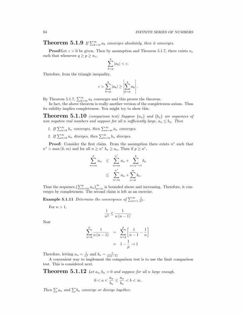
84 INFINITE SERIES OF NUMBERS
Theorem 5.1.9 If∑∞
k=m ak converges absolutely, then it converges.
Proof:Let ε > 0 be given. Then by assumption and Theorem 5.1.7, there exists nεsuch that whenever q ≥ p ≥ nε,
q∑k=p
|ak| < ε.
Therefore, from the triangle inequality,
ε >
q∑k=p
|ak| ≥
∣∣∣∣∣∣q∑
k=p
ak
∣∣∣∣∣∣ .By Theorem 5.1.7,
∑∞k=m ak converges and this proves the theorem.
In fact, the above theorem is really another version of the completeness axiom. Thusits validity implies completeness. You might try to show this.
Theorem 5.1.10 (comparison test) Suppose {an} and {bn} are sequences ofnon negative real numbers and suppose for all n sufficiently large, an ≤ bn. Then
1. If∑∞
n=k bn converges, then∑∞
n=m an converges.
2. If∑∞
n=k an diverges, then∑∞
n=m bn diverges.
Proof: Consider the first claim. From the assumption there exists n∗ such thatn∗ > max (k,m) and for all n ≥ n∗ bn ≥ an. Then if p ≥ n∗,
p∑n=m
an ≤n∗∑
n=m
an +k∑
n=n∗+1
bn
≤n∗∑
n=m
an +∞∑
n=k
bn.
Thus the sequence,{∑p
n=m an}∞p=m
is bounded above and increasing. Therefore, it con-verges by completeness. The second claim is left as an exercise.
Example 5.1.11 Determine the convergence of∑∞
n=11n2 .
For n > 1,1
n2≤ 1
n (n− 1).
Nowp∑
n=2
1
n (n− 1)=
p∑n=2
[1
n− 1− 1
n
]= 1− 1
p→ 1
Therefore, letting an = 1n2 and bn = 1
n(n−1)
A convenient way to implement the comparison test is to use the limit comparisontest. This is considered next.
Theorem 5.1.12 Let an, bn > 0 and suppose for all n large enough,
0 < a <anbn≤ anbn
< b <∞.
Then∑an and
∑bn converge or diverge together.
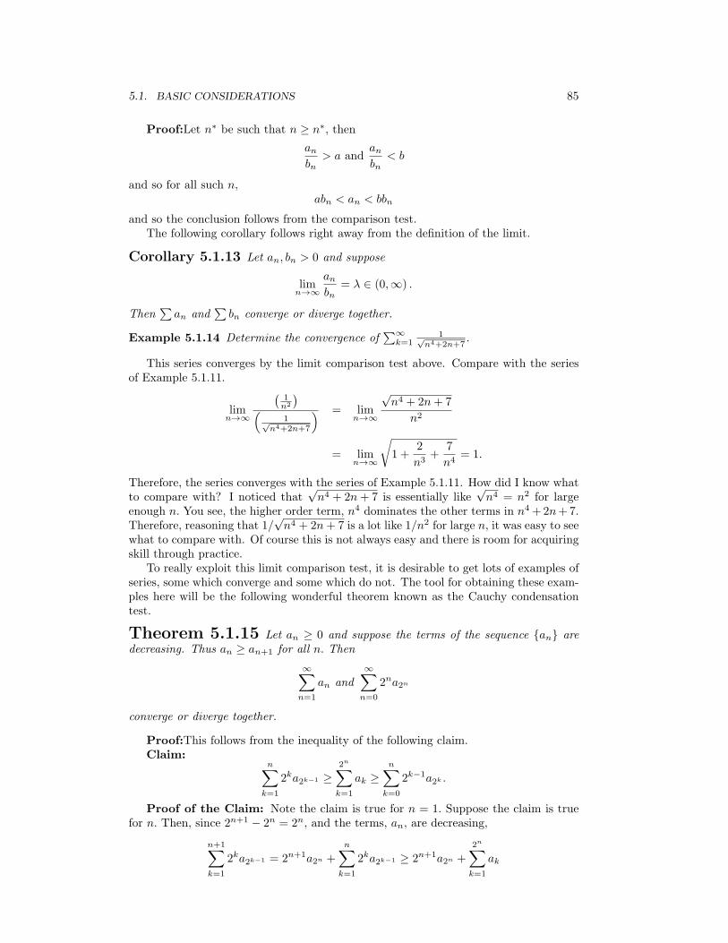
5.1. BASIC CONSIDERATIONS 85
Proof:Let n∗ be such that n ≥ n∗, thenanbn
> a andanbn
< b
and so for all such n,abn < an < bbn
and so the conclusion follows from the comparison test.The following corollary follows right away from the definition of the limit.
Corollary 5.1.13 Let an, bn > 0 and suppose
limn→∞
anbn
= λ ∈ (0,∞) .
Then∑an and
∑bn converge or diverge together.
Example 5.1.14 Determine the convergence of∑∞
k=11√
n4+2n+7.
This series converges by the limit comparison test above. Compare with the seriesof Example 5.1.11.
limn→∞
(1n2
)(1√
n4+2n+7
) = limn→∞
√n4 + 2n+ 7
n2
= limn→∞
√1 +
2
n3+
7
n4= 1.
Therefore, the series converges with the series of Example 5.1.11. How did I know whatto compare with? I noticed that
√n4 + 2n+ 7 is essentially like
√n4 = n2 for large
enough n. You see, the higher order term, n4 dominates the other terms in n4 +2n+7.Therefore, reasoning that 1/
√n4 + 2n+ 7 is a lot like 1/n2 for large n, it was easy to see
what to compare with. Of course this is not always easy and there is room for acquiringskill through practice.
To really exploit this limit comparison test, it is desirable to get lots of examples ofseries, some which converge and some which do not. The tool for obtaining these exam-ples here will be the following wonderful theorem known as the Cauchy condensationtest.
Theorem 5.1.15 Let an ≥ 0 and suppose the terms of the sequence {an} aredecreasing. Thus an ≥ an+1 for all n. Then
∞∑n=1
an and∞∑
n=0
2na2n
converge or diverge together.
Proof:This follows from the inequality of the following claim.Claim:
n∑k=1
2ka2k−1 ≥2n∑k=1
ak ≥n∑
k=0
2k−1a2k .
Proof of the Claim: Note the claim is true for n = 1. Suppose the claim is truefor n. Then, since 2n+1 − 2n = 2n, and the terms, an, are decreasing,
n+1∑k=1
2ka2k−1 = 2n+1a2n +
n∑k=1
2ka2k−1 ≥ 2n+1a2n +
2n∑k=1
ak

86 INFINITE SERIES OF NUMBERS
≥2n+1∑k=1
ak ≥ 2na2n+1 +2n∑k=1
ak ≥ 2na2n+1 +n∑
k=0
2k−1a2k =n+1∑k=0
2k−1a2k .
Example 5.1.16 Determine the convergence of∑∞
k=11kp where p is a positive number.
These are called the p series.
Let an = 1np . Then a2n =
(12p
)n. From the Cauchy condensation test the two series
∞∑n=1
1
npand
∞∑n=0
2n(
1
2p
)n
=∞∑
n=0
(2(1−p)
)nconverge or diverge together. If p > 1, the last series above is a geometric series havingcommon ratio less than 1 and so it converges. If p ≤ 1, it is still a geometric series butin this case the common ratio is either 1 or greater than 1 so the series diverges. Itfollows that the p series converges if p > 1 and diverges if p ≤ 1. In particular,
∑∞n=1 n
−1
diverges while∑∞
n=1 n−2 converges.
Example 5.1.17 Determine the convergence of∑∞
k=11√
n2+100n.
Use the limit comparison test.
limn→∞
(1n
)(1√
n2+100n
) = 1
and so this series diverges with∑∞
k=11k .
Sometimes it is good to be able to say a series does not converge. The nth term testgives such a condition which is sufficient for this. It is really a corollary of Theorem5.1.7.
Theorem 5.1.18 If∑∞
n=m an converges, then limn→∞ an = 0.
Proof:Apply Theorem 5.1.7 to conclude that
limn→∞
an = limn→∞
n∑k=n
ak = 0.
It is very important to observe that this theorem goes only in one direction. That is,you cannot conclude the series converges if limn→∞ an = 0. If this happens, you don’tknow anything from this information. Recall limn→∞ n−1 = 0 but
∑∞n=1 n
−1 diverges.The following picture is descriptive of the situation.
∑an converges
lim an = 0
an = n−1
5.2 Exercises
1. Determine whether the following series converge and give reasons for your answers.
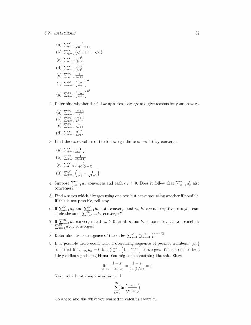
5.2. EXERCISES 87
(a)∑∞
n=11√
n2+n+1
(b)∑∞
n=1
(√n+ 1−
√n)
(c)∑∞
n=1(n!)2
(2n)!
(d)∑∞
n=1(2n)!
(n!)2
(e)∑∞
n=11
2n+2
(f)∑∞
n=1
(n
n+1
)n(g)
∑∞n=1
(n
n+1
)n2
2. Determine whether the following series converge and give reasons for your answers.
(a)∑∞
n=12n+nn2n
(b)∑∞
n=12n+nn22n
(c)∑∞
n=1n
2n+1
(d)∑∞
n=1n100
1.01n
3. Find the exact values of the following infinite series if they converge.
(a)∑∞
k=31
k(k−2)
(b)∑∞
k=11
k(k+1)
(c)∑∞
k=31
(k+1)(k−2)
(d)∑N
k=1
(1√k− 1√
k+1
)4. Suppose
∑∞k=1 ak converges and each ak ≥ 0. Does it follow that
∑∞k=1 a
2k also
converges?
5. Find a series which diverges using one test but converges using another if possible.If this is not possible, tell why.
6. If∑∞
n=1 an and∑∞
n=1 bn both converge and an, bn are nonnegative, can you con-clude the sum,
∑∞n=1 anbn converges?
7. If∑∞
n=1 an converges and an ≥ 0 for all n and bn is bounded, can you conclude∑∞n=1 anbn converges?
8. Determine the convergence of the series∑∞
n=1
(∑nk=1
1k
)−n/2.
9. Is it possible there could exist a decreasing sequence of positive numbers, {an}such that limn→∞ an = 0 but
∑∞n=1
(1− an+1
an
)converges? (This seems to be a
fairly difficult problem.)Hint: You might do something like this. Show
limx→1
1− x− ln (x)
=1− x
ln (1/x)= 1
Next use a limit comparison test with
∞∑n=1
ln
(anan+1
)Go ahead and use what you learned in calculus about ln.
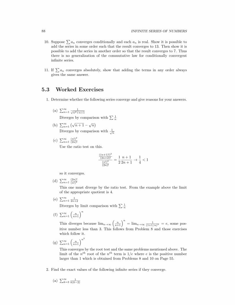
88 INFINITE SERIES OF NUMBERS
10. Suppose∑an converges conditionally and each an is real. Show it is possible to
add the series in some order such that the result converges to 13. Then show it ispossible to add the series in another order so that the result converges to 7. Thusthere is no generalization of the commutative law for conditionally convergentinfinite series.
11. If∑an converges absolutely, show that adding the terms in any order always
gives the same answer.
5.3 Worked Exercises
1. Determine whether the following series converge and give reasons for your answers.
(a)∑∞
n=11√
n2+n+1
Diverges by comparison with∑
1n
(b)∑∞
n=1
(√n+ 1−
√n)
Diverges by comparison with 1√n
(c)∑∞
n=1(n!)2
(2n)!
Use the ratio test on this.
((n+1)!)2
(2n+2)!
(n!)2
(2n)!
=1
2
n+ 1
2n+ 1→ 1
4< 1
so it converges.
(d)∑∞
n=1(2n)!
(n!)2
This one must diverge by the ratio test. From the example above the limitof the appropriate quotient is 4.
(e)∑∞
n=11
2n+2
Diverges by limit comparison with∑
1n
(f)∑∞
n=1
(n
n+1
)nThis diverges because limn→∞
(n
n+1
)n= limn→∞
1(1+1/n)n = e, some pos-
itive number less than 3. This follows from Problem 8 and those exerciseswhich follow it.
(g)∑∞
n=1
(n
n+1
)n2
This converges by the root test and the same problems mentioned above. Thelimit of the nth root of the nth term is 1/e where e is the positive numberlarger than 1 which is obtained from Problems 8 and 10 on Page 55.
2. Find the exact values of the following infinite series if they converge.
(a)∑∞
k=31
k(k−2)

5.3. WORKED EXERCISES 89
1k(k−2) =
12(k−2) −
12k and so
n∑k=3
1
k (k − 2)=
n∑k=3
(1
2 (k − 2)− 1
2k
)
=
n−2∑k=1
1
2k−
n∑k=3
1
2k
=1
2+
1
4− 1
2n− 1
2 (n− 1)
and this converges to 3/4.
(b)∑∞
k=11
k(k+1)
Do this one the same way.∑∞
k=11
k(k+1) = 1
(c)∑∞
k=31
(k+1)(k−2)
This one also can be done the same way. 1(k+1)(k−2) = − 1
3(k+1) + 13(k−2) .
Then writing the partial sums and taking a limit yields∑∞
k=31
(k+1)(k−2) =1118 .
(d)∑∞
k=1
(1√k− 1√
k+1
)N∑
k=1
(1√k− 1√
k + 1
)=
N∑k=1
1√k−
N+1∑k=2
1√k
= 1− 1√N + 1
→ 1.
3. Suppose∑∞
k=1 ak converges and each ak ≥ 0. Does it follow that∑∞
k=1 a2k also
converges?
Yes it does. Eventually ak < 1 and so a2k < ak. Thus the tail of∑∞
k=1 a2k is
dominated by the tail of∑∞
k=1 ak.
4. Find a series which diverges using one test but converges using another if possible.If this is not possible, tell why.
A series either converges or diverges. The tests are there to determine whichtakes place. Therefore, it makes no sense to say a series diverges by one test andconverges by another.
5. If∑∞
n=1 an and∑∞
n=1 bn both converge and an, bn are nonnegative, can you con-clude the sum,
∑∞n=1 anbn converges?
Yes you can. For large n, 0 ≤ anbn ≤ an and∑an is given to converge.
6. If∑∞
n=1 an converges and an ≥ 0 for all n and bn is bounded, can you conclude∑∞n=1 anbn converges?
Yes, you can conclude this. |anbn| ≤ C |an| and it is given that∑|an| converges.
7. Determine the convergence of the series∑∞
n=1
(∑nk=1
1k
)−n/2.
For n large enough,∑n
k=11k > 2 and so(
n∑k=1
1
k
)−n/2
≤ 2−n/2
and∑
2−n/2 converges by the root test. Therefore, the given series converges.
90 INFINITE SERIES OF NUMBERS
8. Is it possible there could exist a decreasing sequence of positive numbers, {an}such that limn→∞ an = 0 but
∑∞n=1
(1− an+1
an
)converges? (This seems to be a
fairly difficult problem.)Hint: You might do something like this. Show
limx→1
1− x− ln (x)
=1− x
ln (1/x)= 1
Next use a limit comparison test with
∞∑n=1
ln
(anan+1
)Go ahead and use what you learned in calculus about ln.
It is not possible. In case lim inf an+1
an< 1, the series diverges by the nth term
test. In case lim inf an+1
an= 1, then since an+1
an≤ 1, lim sup an+1
an= 1 also and so
lim an+1
an= 1. Then it follows from the above limit, the convergence properties of∑(
1− an+1
an
)are the same as those of
∑ln(
an
an+1
)and
N∑n=1
ln
(anan+1
)=
N∑k=1
ln (an)− ln (an+1) = ln (a1)− ln (aN+1)
and it is given that an → 0 so the partial sums are unbounded.
9. Suppose∑an converges conditionally and each an is real. Show it is possible to
add the series in some order such that the result converges to 13. Then show it ispossible to add the series in another order so that the result converges to 7. Thusthere is no generalization of the commutative law for conditionally convergentinfinite series.
Let a+n = 12 (|an|+ an) while a
−n = 1
2 (|an| − an) . Thus an = a+n − a−n . It followsthat
∑n a
+n = ∞ =
∑n a
−n . Of course each a+n equals either 0 or an depending
on whether an is positive. The same holds for a−n . Also a+n → 0 and a−n → 0. Addjust enough positive terms till you exceed 7. Then, starting at the beginning addenough negative terms till you get below 7 then add positive terms till you getabove 7 etc. The resulting series must converge to 7 because you use more andmore terms and an → 0.
10. If∑an converges absolutely, show that adding the terms in any order always
gives the same answer.
Let θ : N→ N be one to one and onto. Consider∑∞
n=1 aθ(n). By absolute conver-gence, there exists an N such that
∞∑k=N
|ak| < ε
Then choose M large enough that {1, 2, · · · , N − 1} ⊆ {θ (1) , θ (2) , · · · , θ (M)} .Then ∣∣∣∣∣∣
N−1∑j=1
aj −M∑j=1
aθ(j)
∣∣∣∣∣∣ ≤∞∑
k=N
|ak| < ε
5.4. MORE TESTS FOR CONVERGENCE 91
Therefore, ∣∣∣∣∣∣M∑j=1
aθ(j) −∞∑j=1
aj
∣∣∣∣∣∣ ≤∣∣∣∣∣∣M∑j=1
aθ(j) −N−1∑j=1
aj
∣∣∣∣∣∣+∣∣∣∣∣
∞∑k=N
ak
∣∣∣∣∣< ε+
∞∑k=N
|ak| < 2ε
since ε is arbitrary, this has shown that
limM→∞
M∑j=1
aθ(j) =∞∑j=1
aj
5.4 More Tests For Convergence
5.4.1 Convergence Because Of Cancellation
So far, the tests for convergence have been applied to non negative terms only. Some-times, a series converges, not because the terms of the series get small fast enough, butbecause of cancellation taking place between positive and negative terms. A discussionof this involves some simple algebra.
Let {an} and {bn} be sequences and let
An ≡n∑
k=1
ak, A−1 ≡ A0 ≡ 0.
Then if p < q
q∑n=p
anbn =
q∑n=p
bn (An −An−1) =
q∑n=p
bnAn −q∑
n=p
bnAn−1
=
q∑n=p
bnAn −q−1∑
n=p−1
bn+1An = bqAq − bpAp−1 +
q−1∑n=p
An (bn − bn+1) (5.6)
This formula is called the partial summation formula.
Theorem 5.4.1 (Dirichlet’s test) Suppose An is bounded and limn→∞ bn = 0,with bn ≥ bn+1 for all n. Then
∞∑n=1
anbn
converges.
Proof:This follows quickly from Theorem 5.1.7. Indeed, letting |An| ≤ C, andusing the partial summation formula above along with the assumption that the bn aredecreasing, ∣∣∣∣∣
q∑n=p
anbn
∣∣∣∣∣ =∣∣∣∣∣bqAq − bpAp−1 +
q−1∑n=p
An (bn − bn+1)
∣∣∣∣∣≤ C (|bq|+ |bp|) + C
q−1∑n=p
(bn − bn+1)
= C (|bq|+ |bp|) + C (bp − bq)and by assumption, this last expression is small whenever p and q are sufficiently large.This proves the theorem.
92 INFINITE SERIES OF NUMBERS
Definition 5.4.2 If bn > 0 for all n, a series of the form∑
k (−1)kbk or∑
k (−1)k−1
bk is known as an alternating series.
The following corollary is known as the alternating series test.
Corollary 5.4.3 (alternating series test) If limn→∞ bn = 0, with bn ≥ bn+1, then∑∞n=1 (−1)
nbn converges.
Proof:Let an = (−1)n . Then the partial sums of∑
n an are bounded and so Theo-rem 5.4.1 applies.
In the situation of Corollary 5.4.3 there is a convenient error estimate available.
Theorem 5.4.4 Let bn > 0 for all n such that bn ≥ bn+1 for all n and limn→∞ bn =0 and consider either
∑∞n=1 (−1)
nbn or
∑∞n=1 (−1)
n−1bn. Then∣∣∣∣∣
∞∑n=1
(−1)n bn −N∑
n=1
(−1)n bn
∣∣∣∣∣ ≤ |bN+1| ,∣∣∣∣∣∞∑
n=1
(−1)n−1bn −
N∑n=1
(−1)n−1bn
∣∣∣∣∣ ≤ |bN+1|
See Problem 9 on Page 100 for an outline of the proof of this theorem along withanother way to prove the alternating series test.
Example 5.4.5 How many terms must I take in the sum,∑∞
n=1 (−1)n 1
n2+1 to be closer
than 110 to
∑∞n=1 (−1)
n 1n2+1?
From Theorem 5.4.4, I need to find n such that 1n2+1 ≤
110 and then n − 1 is the
desired value. Thus n = 3 and so∣∣∣∣∣∞∑
n=1
(−1)n 1
n2 + 1−
2∑n=1
(−1)n 1
n2 + 1
∣∣∣∣∣ ≤ 1
10
Definition 5.4.6 A series∑an is said to converge absolutely if
∑|an| con-
verges. It is said to converge conditionally if∑|an| fails to converge but
∑an converges.
Thus the alternating series or more general Dirichlet test can determine convergenceof series which converge conditionally.
5.4.2 Ratio And Root Tests
A favorite test for convergence is the ratio test. This is discussed next. It is at theother extreme from the alternating series test, being completely oblivious to any sort ofcancellation. It only gives absolute convergence or spectacular divergence.
Theorem 5.4.7 Suppose |an| > 0 for all n and suppose
limn→∞
|an+1||an|
= r.
Then∞∑
n=1
an
diverges if r > 1converges absolutely if r < 1test fails if r = 1
.
5.4. MORE TESTS FOR CONVERGENCE 93
Proof:Suppose r < 1. Then there exists n1 such that if n ≥ n1, then
0 <
∣∣∣∣an+1
an
∣∣∣∣ < R
where r < R < 1. Then|an+1| < R |an|
for all such n. Therefore,
|an1+p| < R |an1+p−1| < R2 |an1+p−2| < · · · < Rp |an1 | (5.7)
and so if m > n, then |am| < Rm−n1 |an1 | . By the comparison test and the theorem ongeometric series,
∑|an| converges. This proves the convergence part of the theorem.
To verify the divergence part, note that if r > 1, then 5.7 can be turned around forsome R > 1. Showing limn→∞ |an| = ∞. Since the nth term fails to converge to 0, itfollows the series diverges.
To see the test fails if r = 1, consider∑n−1 and
∑n−2. The first series diverges
while the second one converges but in both cases, r = 1. (Be sure to check this lastclaim.)
The ratio test is very useful for many different examples but it is somewhat unsatis-factory mathematically. One reason for this is the assumption that an > 0, necessitatedby the need to divide by an, and the other reason is the possibility that the limit mightnot exist. The next test, called the root test removes both of these objections. Beforepresenting this test, it is necessary to first prove the existence of the pth root of anypositive number.
Lemma 5.4.8 Let α > 0 be any nonnegative number and let p ∈ N. Then α1/p
exists. This is the unique positive number which when raised to the pth power gives α.
Proof: Consider the function f (x) ≡ xp − α. Then there exists b1 such thatf (b1) > 0 and a1 such that f (a1) < 0. (Why?) Now cut the interval [a1, b1] into twoclosed intervals of equal length. Let [a2, b2] be one of these which has f (a2) f (b2) ≤ 0.Now do for [a2, b2] the same thing which was done to get [a2, b2] from [a1, b1]. Continuethis way obtaining a sequence of nested intervals [ak, bk] with the property that
bk − ak = 21−k (b1 − a1) .
By the nested interval theorem, there exists a unique point x in all these intervals.Generalizing Theorem 4.5.6 slightly to include the product of of the terms of finitelymany sequences, it follows from Theorem 4.5.11 that
f (x) f (x) = limk→∞
f (ak) f (bk) ≤ 0
Hence f (x) = 0. This proves the lemma.
Theorem 5.4.9 Suppose |an|1/n < R < 1 for all n sufficiently large. Then
∞∑n=1
an converges absolutely.
If there are infinitely many values of n such that |an|1/n ≥ 1, then
∞∑n=1
an diverges.

94 INFINITE SERIES OF NUMBERS
Proof: Suppose first that |an|1/n < R < 1 for all n sufficiently large. Say this holdsfor all n ≥ nR. Then for such n,
n√|an| < R.
Therefore, for such n,|an| ≤ Rn
and so the comparison test with a geometric series applies and gives absolute convergenceas claimed.
Next suppose |an|1/n ≥ 1 for infinitely many values of n. Then for those values of n,|an| ≥ 1 and so the series fails to converge by the nth term test.
Stated more succinctly the condition for the root test is this: Let
r = lim supn→∞
|an|1/n
then∞∑
k=m
ak
converges absolutely if r < 1test fails if r = 1diverges if r > 1
A special case occurs when the limit exists.
Corollary 5.4.10 Suppose limn→∞ |an|1/n exists and equals r. Then
∞∑k=m
ak
converges absolutely if r < 1test fails if r = 1diverges if r > 1
Proof:The first and last alternatives follow from Theorem 5.4.9. To see the testfails if r = 1, consider the two series
∑∞n=1
1n and
∑∞n=1
1n2 both of which have r = 1
but having different convergence properties.
5.5 Double Series
Sometimes it is required to consider double series which are of the form
∞∑k=m
∞∑j=m
ajk ≡∞∑
k=m
∞∑j=m
ajk
.
In other words, first sum on j yielding something which depends on k and then sumthese. The major consideration for these double series is the question of when
∞∑k=m
∞∑j=m
ajk =∞∑
j=m
∞∑k=m
ajk.
In other words, when does it make no difference which subscript is summed over first?In the case of finite sums there is no issue here. You can always write
M∑k=m
N∑j=m
ajk =
N∑j=m
M∑k=m
ajk
because addition is commutative. However, there are limits involved with infinite sumsand the interchange in order of summation involves taking limits in a different order.Therefore, it is not always true that it is permissible to interchange the two sums. A

5.5. DOUBLE SERIES 95
general rule of thumb is this: If something involves changing the order in which twolimits are taken, you may not do it without agonizing over the question. In general,limits foul up algebra and also introduce things which are counter intuitive. Here is anexample. This example is a little technical. It is placed here just to prove conclusivelythere is a question which needs to be considered.
Example 5.5.1 Consider the following picture which depicts some of the ordered pairs(m,n) where m,n are positive integers.
0 q0 q
0 q0 q
0 q0 q
0 q
-c q-c q
-c q-c q
-c q-c q
a qc q
c qc q
c qc q
b q0 q
0 q0 q
0 q0 q
0 q0 q
0 q0 q
0 q0 q
0 q0 q
0 q0 q
0 q0 q
0 q0 q
0 q0 q
0 q0 q
0 q0 q
0 q
0 q0 q
0 q0 q
0 q0 q
0 q0 q
0 q0 q
The numbers next to the point are the values of amn. You see ann = 0 for all n,a21 = a, a12 = b, amn = c for (m,n) on the line y = 1 + x whenever m > 1, andamn = −c for all (m,n) on the line y = x− 1 whenever m > 2.
Then∑∞
m=1 amn = a if n = 1,∑∞
m=1 amn = b−c if n = 2 and if n > 2,∑∞
m=1 amn =0. Therefore,
∞∑n=1
∞∑m=1
amn = a+ b− c.
Next observe that∑∞
n=1 amn = b ifm = 1,∑∞
n=1 amn = a+c ifm = 2, and∑∞
n=1 amn =0 if m > 2. Therefore,
∞∑m=1
∞∑n=1
amn = b+ a+ c
and so the two sums are different. Moreover, you can see that by assigning differentvalues of a, b, and c, you can get an example for any two different numbers desired.
Don’t become upset by this. It happens because, as indicated above, limits are takenin two different orders. An infinite sum always involves a limit and this illustrates whyyou must always remember this. This example in no way violates the commutative lawof addition which has nothing to do with limits. However, it turns out that if aij ≥ 0for all i, j, then you can always interchange the order of summation. This is shown nextand is based on the following lemma. First, some notation should be discussed.
Definition 5.5.2 Let f (a, b) ∈ [−∞,∞] for a ∈ A and b ∈ B where A,Bare sets which means that f (a, b) is either a number, ∞, or −∞. The symbol, +∞is interpreted as a point out at the end of the number line which is larger than everyreal number. Of course there is no such number. That is why it is called ∞. Thesymbol, −∞ is interpreted similarly. Then supa∈A f (a, b) means sup (Sb) where Sb ≡{f (a, b) : a ∈ A} .
96 INFINITE SERIES OF NUMBERS
Unlike limits, you can take the sup in different orders.
Lemma 5.5.3 Let f (a, b) ∈ [−∞,∞] for a ∈ A and b ∈ B where A,B are sets.Then
supa∈A
supb∈B
f (a, b) = supb∈B
supa∈A
f (a, b) .
Proof: Note that for all a, b, f (a, b) ≤ supb∈B supa∈A f (a, b) and therefore, for alla, supb∈B f (a, b) ≤ supb∈B supa∈A f (a, b). Therefore,
supa∈A
supb∈B
f (a, b) ≤ supb∈B
supa∈A
f (a, b) .
Repeat the same argument interchanging a and b, to get the conclusion of the lemma.
Lemma 5.5.4 If {An} is an increasing sequence in [−∞,∞], then
sup {An} = limn→∞
An.
Proof: Let sup ({An : n ∈ N}) = r. In the first case, suppose r < ∞. Then lettingε > 0 be given, there exists n such that An ∈ (r − ε, r]. Since {An} is increasing, itfollows if m > n, then r − ε < An ≤ Am ≤ r and so limn→∞An = r as claimed. Inthe case where r = ∞, then if a is a real number, there exists n such that An > a.Since {Ak} is increasing, it follows that if m > n, Am > a. But this is what is meantby limn→∞An =∞. The other case is that r = −∞. But in this case, An = −∞ for alln and so limn→∞An = −∞.
Theorem 5.5.5 Let aij ≥ 0. Then
∞∑i=1
∞∑j=1
aij =∞∑j=1
∞∑i=1
aij .
Proof: First note there is no trouble in defining these sums because the aij are allnonnegative. If a sum diverges, it only diverges to ∞ and so ∞ is the value of the sum.Next note that
∞∑j=r
∞∑i=r
aij ≥ supn
∞∑j=r
n∑i=r
aij
because for all j,∞∑i=r
aij ≥n∑
i=r
aij .
Therefore,∞∑j=r
∞∑i=r
aij ≥ supn
∞∑j=r
n∑i=r
aij = supn
limm→∞
m∑j=r
n∑i=r
aij
= supn
limm→∞
n∑i=r
m∑j=r
aij = supn
n∑i=r
limm→∞
m∑j=r
aij
= supn
n∑i=r
∞∑j=r
aij = limn→∞
n∑i=r
∞∑j=r
aij =
∞∑i=r
∞∑j=r
aij
Interchanging the i and j in the above argument proves the theorem.The following is the fundamental result on double sums.
5.5. DOUBLE SERIES 97
Theorem 5.5.6 Let aij ∈ F and suppose
∞∑i=r
∞∑j=r
|aij | <∞ .
Then∞∑i=r
∞∑j=r
aij =∞∑j=r
∞∑i=r
aij
and every infinite sum encountered in the above equation converges.
Proof:By Theorem 5.5.5∞∑j=r
∞∑i=r
|aij | =∞∑i=r
∞∑j=r
|aij | <∞
Therefore, for each j,∑∞
i=r |aij | < ∞ and for each i,∑∞
j=r |aij | < ∞. By Theorem
5.1.9 on Page 84,∑∞
i=r aij ,∑∞
j=r aij both converge, the first one for every j and thesecond for every i. Also,
∞∑j=r
∣∣∣∣∣∞∑i=r
aij
∣∣∣∣∣ ≤∞∑j=r
∞∑i=r
|aij | <∞
and∞∑i=r
∣∣∣∣∣∣∞∑j=r
aij
∣∣∣∣∣∣ ≤∞∑i=r
∞∑j=r
|aij | <∞
so by Theorem 5.1.9 again,∞∑j=r
∞∑i=r
aij ,∞∑i=r
∞∑j=r
aij
both exist. It only remains to verify they are equal. By similar reasoning you canreplace aij with Re aij or with Im aij in the above and the two sums will exist.
The real part of a finite sum of complex numbers equals the sum of the real parts.Then passing to a limit, it follows
Re∞∑j=r
∞∑i=r
aij =∞∑j=r
∞∑i=r
Re aij
and similarly,
Im∞∑i=r
∞∑j=r
aij =∞∑i=r
∞∑j=r
Im aij
Note 0 ≤ (|aij |+Re aij) ≤ 2 |aij | . Therefore, by Theorem 5.5.5 and Theorem 5.1.5 onPage 82
∞∑j=r
∞∑i=r
|aij |+∞∑j=r
∞∑i=r
Re aij =
∞∑j=r
∞∑i=r
(|aij |+Re aij)
=∞∑i=r
∞∑j=r
(|aij |+Re aij)
=
∞∑i=r
∞∑j=r
|aij |+∞∑i=r
∞∑j=r
Re aij
=∞∑j=r
∞∑i=r
|aij |+∞∑i=r
∞∑j=r
Re aij
98 INFINITE SERIES OF NUMBERS
and so
Re∞∑j=r
∞∑i=r
aij =∞∑j=r
∞∑i=r
Re aij =∞∑i=r
∞∑j=r
Re aij = Re∞∑i=r
∞∑j=r
aij
Similar reasoning applies to the imaginary parts. Since the real and imaginary parts ofthe two series are equal, it follows the two series are equal. This proves the theorem.
One of the most important applications of this theorem is to the problem of multi-plication of series.
Definition 5.5.7 Let∑∞
i=r ai and∑∞
i=r bi be two series. For n ≥ r, define
cn ≡n∑
k=r
akbn−k+r.
The series∑∞
n=r cn is called the Cauchy product of the two series.
It isn’t hard to see where this comes from. Formally write the following in the caser = 0:
(a0 + a1 + a2 + a3 · · · ) (b0 + b1 + b2 + b3 · · · )
and start multiplying in the usual way. This yields
a0b0 + (a0b1 + b0a1) + (a0b2 + a1b1 + a2b0) + · · ·
and you see the expressions in parentheses above are just the cn for n = 0, 1, 2, · · · .Therefore, it is reasonable to conjecture that
∞∑i=r
ai
∞∑j=r
bj =∞∑
n=r
cn
and of course there would be no problem with this in the case of finite sums but in thecase of infinite sums, it is necessary to prove a theorem. The following is a special caseof Merten’s theorem.
Theorem 5.5.8 Suppose∑∞
i=r ai and∑∞
j=r bj both converge absolutely1. Then
( ∞∑i=r
ai
) ∞∑j=r
bj
=
∞∑n=r
cn
where
cn =
n∑k=r
akbn−k+r.
Proof: Let pnk = 1 if r ≤ k ≤ n and pnk = 0 if k > n. Then
cn =∞∑k=r
pnkakbn−k+r.
1Actually, it is only necessary to assume one of the series converges and the other converges abso-lutely. This is known as Merten’s theorem and may be read in the 1974 book by Apostol listed in thebibliography.

5.6. EXERCISES 99
Also,
∞∑k=r
∞∑n=r
pnk |ak| |bn−k+r| =∞∑k=r
|ak|∞∑
n=r
pnk |bn−k+r|
=
∞∑k=r
|ak|∞∑
n=k
|bn−k+r|
=∞∑k=r
|ak|∞∑
n=k
∣∣bn−(k−r)
∣∣=
∞∑k=r
|ak|∞∑
m=r
|bm| <∞.
Therefore, by Theorem 5.5.6
∞∑n=r
cn =
∞∑n=r
n∑k=r
akbn−k+r =
∞∑n=r
∞∑k=r
pnkakbn−k+r
=∞∑k=r
ak
∞∑n=r
pnkbn−k+r =∞∑k=r
ak
∞∑n=k
bn−k+r
=
∞∑k=r
ak
∞∑m=r
bm
and this proves the theorem.
5.6 Exercises
1. Determine whether the following series converge absolutely, conditionally, or notat all and give reasons for your answers.
(a)∑∞
n=1 (−1)n 1√
n2+n+1
(b)∑∞
n=1 (−1)n (√
n+ 1−√n)
(c)∑∞
n=1 (−1)n (n!)2
(2n)!
(d)∑∞
n=1 (−1)n (2n)!
(n!)2
(e)∑∞
n=1(−1)n
2n+2
(f)∑∞
n=1 (−1)n(
nn+1
)n(g)
∑∞n=1 (−1)
n(
nn+1
)n2
2. Determine whether the following series converge absolutely, conditionally, or notat all and give reasons for your answers.
(a)∑∞
n=1 (−1)n 2n+n
n2n
(b)∑∞
n=1 (−1)n 2n+n
n22n
(c)∑∞
n=1 (−1)n n
2n+1
(d)∑∞
n=1 (−1)n 10n
n!
100 INFINITE SERIES OF NUMBERS
(e)∑∞
n=1 (−1)n n100
1.01n
(f)∑∞
n=1 (−1)n 3n
n3
(g)∑∞
n=1 (−1)n n3
3n
(h)∑∞
n=1 (−1)n n3
n!
(i)∑∞
n=1 (−1)n n!
n100
3. Suppose∑∞
n=1 an converges absolutely. Can the same thing be said about∑∞
n=1 a2n?
Explain.
4. A person says a series converges conditionally by the ratio test. Explain why hisstatement is total nonsense.
5. A person says a series diverges by the alternating series test. Explain why hisstatement is total nonsense.
6. Find a series which diverges using one test but converges using another if possible.If this is not possible, tell why.
7. If∑∞
n=1 an and∑∞
n=1 bn both converge, can you conclude the sum,∑∞
n=1 anbnconverges?
8. If∑∞
n=1 an converges absolutely, and bn is bounded, can you conclude∑∞
n=1 anbnconverges? What if it is only the case that
∑∞n=1 an converges?
9. Prove Theorem 5.4.4. Hint: For∑∞
k=1 (−1)nbn, show the odd partial sums are
all at least as small as∑∞
k=1 (−1)nbn and are increasing while the even partial
sums are at least as large as∑∞
k=1 (−1)nbn and are decreasing. Use this to give
another proof of the alternating series test. If you have trouble, see most standardcalculus books.
10. Use Theorem 5.4.4 in the following alternating series to tell how large n must be
so that∣∣∣∑∞
k=1 (−1)kak −
∑nk=1 (−1)
kak
∣∣∣ is no larger than the given number.
(a)∑∞
k=1 (−1)k 1
k , .001
(b)∑∞
k=1 (−1)k 1
k2 , .001
(c)∑∞
k=1 (−1)k−1 1√
k, .001
11. Consider the series∑∞
k=0 (−1)n 1√
n+1. Show this series converges and so it makes
sense to write(∑∞
k=0 (−1)n 1√
n+1
)2. What about the Cauchy product of this
series? Does it even converge? What does this mean about using algebra oninfinite sums as though they were finite sums?
12. Verify Theorem 5.5.8 on the two series∑∞
k=0 2−k and
∑∞k=0 3
−k.
13. You can define infinite series of complex numbers in exactly the same way asinfinite series of real numbers. That is w =
∑∞k=1 zk means: For every ε > 0 there
exists N such that if n ≥ N, then∣∣∣w −∑N
k=1 zk
∣∣∣ < ε. Here the absolute value is
the one which applies to complex numbers. That is, |a+ ib| =√a2 + b2. Show
that if {an} is a decreasing sequence of nonnegative numbers with the propertythat limn→∞ an = 0 and if ω is any complex number which is not equal to 1but which satisfies |ω| = 1, then
∑∞k=1 ω
nan must converge. Note a sequence

5.7. WORKED EXERCISES 101
of complex numbers, {an + ibn} converges to a + ib if and only if an → a andbn → b. See Problem 6 on Page 55. There are quite a few things in this problemyou should think about.
14. Suppose limk→∞ sk = s. Show it follows limn→∞1n
∑nk=1 sk = s.
15. Using Problem 14 show that if∑∞
j=1aj
j converges, then it follows
limn→∞
1
n
n∑j=1
aj = 0.
16. Show that if {pi}∞i=1 are the prime numbers, then∑∞
i=11pi
= ∞. That is, there
are enough primes that the sum of their reciprocals diverges. Hint: Let ϕ (n)denote the number of primes less than equal to n. Then explain why
n∑k=1
1
k≤
ϕ(n)∏k=1
(1 +
1
pk
)≤
ϕ(n)∏k=1
e1/pk = e∑ϕ(n)
k=1 1/pk
and consequently why limn→∞ ϕ (n) =∞ and∑∞
i=11pi
=∞.
5.7 Worked Exercises
1. If∑∞
n=1 an and∑∞
n=1 bn both converge, can you conclude the sum,∑∞
n=1 anbnconverges?
No you can’t. Say an = (−1)n 1n = bn.
2. If∑∞
n=1 an converges absolutely, and bn is bounded, can you conclude∑∞
n=1 anbnconverges? What if it is only the case that
∑∞n=1 an converges?
The first part is all right. However, the second part is not. Let bn = (−1)n andan = (−1)n 1
n .
3. Prove Theorem 5.4.4. Hint: For∑∞
k=1 (−1)nbn, show the odd partial sums are
all at least as small as∑∞
k=1 (−1)nbn and are increasing while the even partial
sums are at least as large as∑∞
k=1 (−1)nbn and are decreasing. Use this to give
another proof of the alternating series test. If you have trouble, see most standardcalculus books.
Denote by Sn the nth partial sum. Then
S2n + (−1)2n+1b2n+1 + b2n+2 = S2n+2
and so since the bn are decreasing, this shows
S2n ≥ S2n+2
Similarly n→ S2n+1 is increasing. Then if k < n,
S2k−1 ≤ S2n−1 ≤ S2n
while if k > n,S2k−1 ≤ S2k ≤ S2n
Thus every odd sum is below every even sum. It follows the even sums convergebecause they form a decreasing sequence which is bounded below. But also,
|S2n − S2n−1| = b2n
102 INFINITE SERIES OF NUMBERS
and so it follows the odd sums also converge to the same thing, S and S is therefore,the unique number between all the odd sums and all the even sums.
|S2n − S| ≤ |S2n − S2n+1| = b2n+1
|S2n+1 − S| ≤ S2n+2 − S2n+1 = b2n+2
and so since n is either even or odd, Sn → S. This also shows that the error is nomore than the absolute value of the next term in the series.
4. Suppose limk→∞ sk = s. Show it follows limn→∞1n
∑nk=1 sk = s.
This was done earlier.
5. Using Problem 14 show that if∑∞
j=1aj
j converges, then it follows
limn→∞
1
n
n∑j=1
aj = 0.
This one is really interesting.
1
n
n∑j=1
aj =1
n
n∑j=1
jajj
=1
n
n∑j=1
j∑i=1
ajj
=1
n
n∑i=1
n∑j=i
ajj
=1
n
n∑i=1
∞∑j=i
ajj− 1
n
n∑i=1
∞∑j=n+1
ajj
(5.8)
Now for n large enough, ∣∣∣∣∣∣∞∑
j=n+1
ajj
∣∣∣∣∣∣ < ε
and so the second term in 5.8 is bounded by ε for all such large n. The first sumconverges to 0 as n→∞ because limi→∞
∑∞j=i
aj
j = 0 so the first term convergesto 0 as n→∞ by the previous problem.
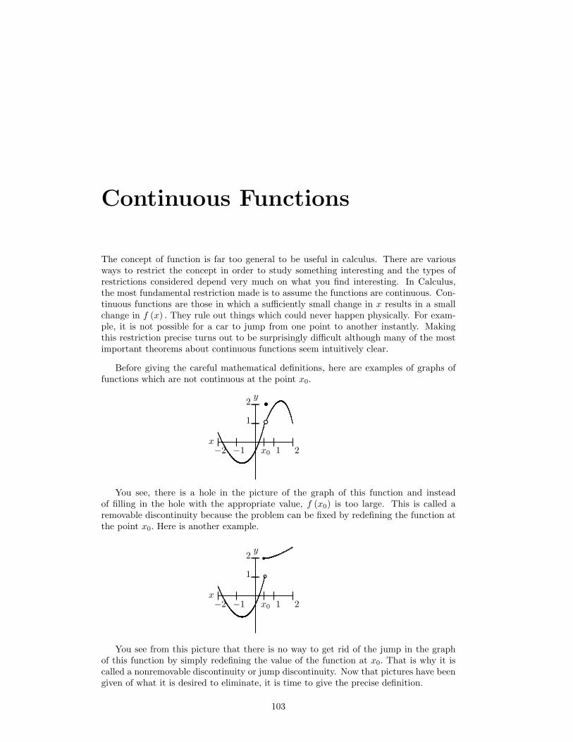
Continuous Functions
The concept of function is far too general to be useful in calculus. There are variousways to restrict the concept in order to study something interesting and the types ofrestrictions considered depend very much on what you find interesting. In Calculus,the most fundamental restriction made is to assume the functions are continuous. Con-tinuous functions are those in which a sufficiently small change in x results in a smallchange in f (x) . They rule out things which could never happen physically. For exam-ple, it is not possible for a car to jump from one point to another instantly. Makingthis restriction precise turns out to be surprisingly difficult although many of the mostimportant theorems about continuous functions seem intuitively clear.
Before giving the careful mathematical definitions, here are examples of graphs offunctions which are not continuous at the point x0.
x
y•cx0 1 2−2 −1
1
2
You see, there is a hole in the picture of the graph of this function and insteadof filling in the hole with the appropriate value, f (x0) is too large. This is called aremovable discontinuity because the problem can be fixed by redefining the function atthe point x0. Here is another example.
x
y rbx0 1 2−2 −1
1
2
You see from this picture that there is no way to get rid of the jump in the graphof this function by simply redefining the value of the function at x0. That is why it iscalled a nonremovable discontinuity or jump discontinuity. Now that pictures have beengiven of what it is desired to eliminate, it is time to give the precise definition.
103
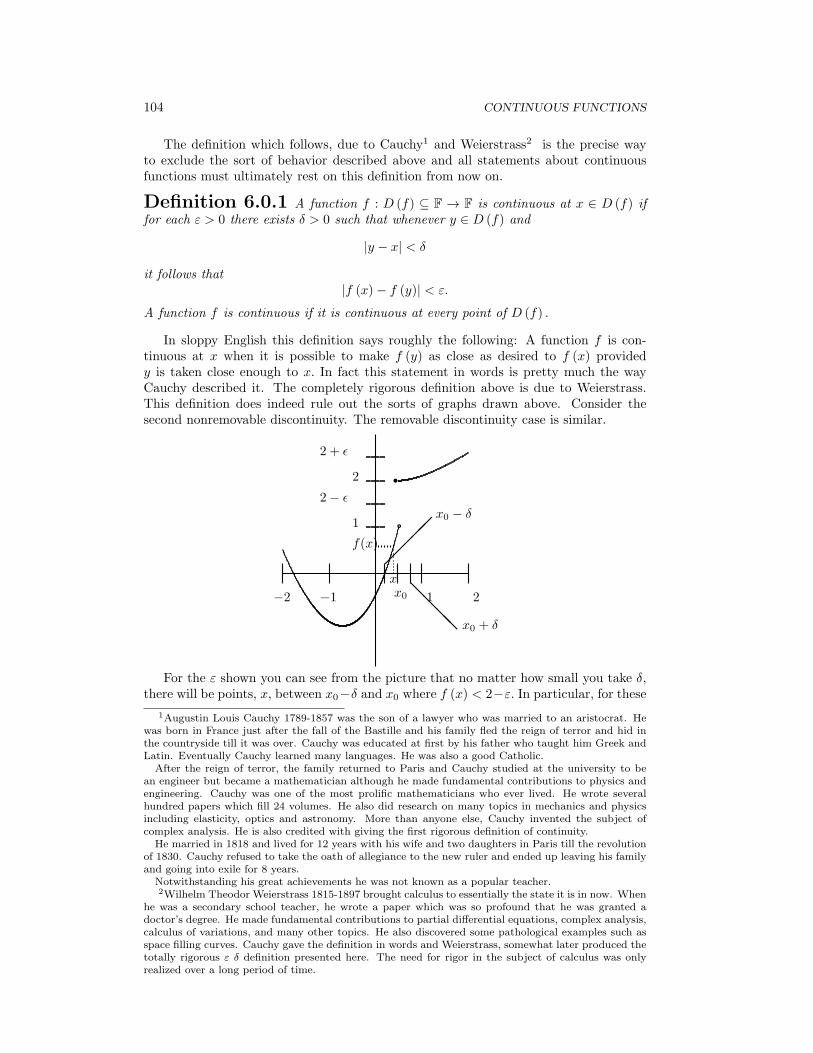
104 CONTINUOUS FUNCTIONS
The definition which follows, due to Cauchy1 and Weierstrass2 is the precise wayto exclude the sort of behavior described above and all statements about continuousfunctions must ultimately rest on this definition from now on.
Definition 6.0.1 A function f : D (f) ⊆ F → F is continuous at x ∈ D (f) iffor each ε > 0 there exists δ > 0 such that whenever y ∈ D (f) and
|y − x| < δ
it follows that|f (x)− f (y)| < ε.
A function f is continuous if it is continuous at every point of D (f) .
In sloppy English this definition says roughly the following: A function f is con-tinuous at x when it is possible to make f (y) as close as desired to f (x) providedy is taken close enough to x. In fact this statement in words is pretty much the wayCauchy described it. The completely rigorous definition above is due to Weierstrass.This definition does indeed rule out the sorts of graphs drawn above. Consider thesecond nonremovable discontinuity. The removable discontinuity case is similar.
2 + ϵ
2− ϵra
x0
x0 + δ
x0 − δ
1 2−2 −1
1
2
f(x)
x@@
@@
����
For the ε shown you can see from the picture that no matter how small you take δ,there will be points, x, between x0−δ and x0 where f (x) < 2−ε. In particular, for these
1Augustin Louis Cauchy 1789-1857 was the son of a lawyer who was married to an aristocrat. Hewas born in France just after the fall of the Bastille and his family fled the reign of terror and hid inthe countryside till it was over. Cauchy was educated at first by his father who taught him Greek andLatin. Eventually Cauchy learned many languages. He was also a good Catholic.
After the reign of terror, the family returned to Paris and Cauchy studied at the university to bean engineer but became a mathematician although he made fundamental contributions to physics andengineering. Cauchy was one of the most prolific mathematicians who ever lived. He wrote severalhundred papers which fill 24 volumes. He also did research on many topics in mechanics and physicsincluding elasticity, optics and astronomy. More than anyone else, Cauchy invented the subject ofcomplex analysis. He is also credited with giving the first rigorous definition of continuity.
He married in 1818 and lived for 12 years with his wife and two daughters in Paris till the revolutionof 1830. Cauchy refused to take the oath of allegiance to the new ruler and ended up leaving his familyand going into exile for 8 years.
Notwithstanding his great achievements he was not known as a popular teacher.2Wilhelm Theodor Weierstrass 1815-1897 brought calculus to essentially the state it is in now. When
he was a secondary school teacher, he wrote a paper which was so profound that he was granted adoctor’s degree. He made fundamental contributions to partial differential equations, complex analysis,calculus of variations, and many other topics. He also discovered some pathological examples such asspace filling curves. Cauchy gave the definition in words and Weierstrass, somewhat later produced thetotally rigorous ε δ definition presented here. The need for rigor in the subject of calculus was onlyrealized over a long period of time.

105
values of x, |f (x)− f (x0)| > ε. Therefore, the definition of continuity given aboveexcludes the situation in which there is a jump in the function. Similar reasoning showsit excludes the removable discontinuity case as well. There are many ways a functioncan fail to be continuous and it is impossible to list them all by drawing pictures. Thisis why it is so important to use the definition. The other thing to notice is that theconcept of continuity as described in the definition is a point property. That is to sayit is a property which a function may or may not have at a single point. Here is anexample.
Example 6.0.2 Let
f (x) =
{x if x is rational0 if x is irrational
.
This function is continuous at x = 0 and nowhere else.
To verify the assertion about the above function, first show it is not continuous atx if x = 0. Take such an x and let ε = |x| /2. Now let δ > 0 be completely arbitrary.In the interval, (x− δ, x+ δ) there are rational numbers, y1 such that |y1| > |x| andirrational numbers, y2. Thus |f (y1)− f (y2)| = |y1| > |x| . If f were continuous at x,there would exist δ > 0 such that for every point, y ∈ (x− δ, x+ δ), |f (y)− f (x)| < ε.But then, letting y1 and y2 be as just described,
|x| < |y1| = |f (y1)− f (y2)|≤ |f (y1)− f (x)|+ |f (x)− f (y2)| < 2ε = |x| ,
which is a contradiction. Since a contradiction is obtained by assuming that f is contin-uous at x, it must be concluded that f is not continuous there. To see f is continuousat 0, let ε > 0 be given and let δ = ε. Then if |y − 0| < δ = ε, Then
|f (y)− f (0)| = 0 if y is irrational
|f (y)− f (0)| = |y| < ε if y is rational.
either way, whenever |y − 0| < δ, it follows |f (y)− f (0)| < ε and so f is continuous atx = 0. How did I know to let δ = ε? That is a very good question. The choice of δ fora particular ε is usually arrived at by using intuition, the actual ε δ argument reducesto a verification that the intuition was correct. Here is another example.
Example 6.0.3 Show the function f (x) = −5x+ 10 is continuous at x = −3.
To do this, note first that f (−3) = 25 and it is desired to verify the conditions forcontinuity. Consider the following.
|−5x+ 10− (25)| = 5 |x− (−3)| .
This allows one to find a suitable δ. If ε > 0 is given, let 0 < δ ≤ 15ε. Then if 0 <
|x− (−3)| < δ, it follows from this inequality that
|−5x+ 10− (25)| = 5 |x− (−3)| < 51
5ε = ε.
Sometimes the determination of δ in the verification of continuity can be a littlemore involved. Here is another example.
Example 6.0.4 Show the function f (x) =√2x+ 12 is continuous at x = 5.

106 CONTINUOUS FUNCTIONS
First note f (5) =√22. Now consider:∣∣∣√2x+ 12−
√22∣∣∣ = ∣∣∣∣ 2x+ 12− 22
√2x+ 12 +
√22
∣∣∣∣=
2√2x+ 12 +
√22|x− 5| ≤ 1
11
√22 |x− 5|
whenever |x− 5| < 1 because for such x,√2x+ 12 > 0. Now let ε > 0 be given. Choose
δ such that 0 < δ ≤ min(1, ε
√222
). Then if |x− 5| < δ, all the inequalities above hold
and ∣∣∣√2x+ 12−√22∣∣∣ ≤ 2√
22|x− 5| < 2√
22
ε√22
2= ε.
Exercise 6.0.5 Show f (x) = −3x2 + 7 is continuous at x = 7.
First observe f (7) = −140. Now∣∣−3x2 + 7− (−140)∣∣ = 3 |x+ 7| |x− 7| ≤ 3 (|x|+ 7) |x− 7| .
If |x− 7| < 1, it follows from the version of the triangle inequality which states ||s| − |t|| ≤|s− t| that |x| < 1 + 7. Therefore, if |x− 7| < 1, it follows that∣∣−3x2 + 7− (−140)
∣∣ ≤ 3 ((1 + 7) + 7) |x− 7|
= 3 (1 + 27) |x− 7| = 84 |x− 7| .
Now let ε > 0 be given. Choose δ such that 0 < δ ≤ min(1, ε
84
). Then for |x− 7| < δ,
it follows ∣∣−3x2 + 7− (−140)∣∣ ≤ 84 |x− 7| < 84
( ε84
)= ε.
The following is a useful theorem which can remove the need to constantly use theε, δ definition given above.
Theorem 6.0.6 The following assertions are valid
1. The function af + bg is continuous at x when f , g are continuous at x ∈ D (f) ∩D (g) and a, b ∈ F.
2. If and f and g are each continuous at x, then fg is continuous at x. If, in additionto this, g (x) = 0, then f/g is continuous at x.
3. If f is continuous at x, f (x) ∈ D (g) ⊆ F, and g is continuous at f (x) ,then g ◦ fis continuous at x.
4. The function f : F→ R, given by f (x) = |x| is continuous.
Proof: First consider 1.) Let ε > 0 be given. By assumption, there exist δ1 > 0such that whenever |x− y| < δ1, it follows |f (x)− f (y)| < ε
2(|a|+|b|+1) and there exists
δ2 > 0 such that whenever |x− y| < δ2, it follows that |g (x)− g (y)| < ε2(|a|+|b|+1) . Then
let 0 < δ ≤ min (δ1, δ2) . If |x− y| < δ, then everything happens at once. Therefore,using the triangle inequality
|af (x) + bf (x)− (ag (y) + bg (y))|
107
≤ |a| |f (x)− f (y)|+ |b| |g (x)− g (y)|
< |a|(
ε
2 (|a|+ |b|+ 1)
)+ |b|
(ε
2 (|a|+ |b|+ 1)
)< ε.
Now consider 2.) There exists δ1 > 0 such that if |y − x| < δ1, then |f (x)− f (y)| <1. Therefore, for such y,
|f (y)| < 1 + |f (x)| .
It follows that for such y,
|fg (x)− fg (y)| ≤ |f (x) g (x)− g (x) f (y)|+ |g (x) f (y)− f (y) g (y)|
≤ |g (x)| |f (x)− f (y)|+ |f (y)| |g (x)− g (y)|≤ (1 + |g (x)|+ |f (y)|) [|g (x)− g (y)|+ |f (x)− f (y)|]≤ (2 + |g (x)|+ |f (x)|) [|g (x)− g (y)|+ |f (x)− f (y)|]
Now let ε > 0 be given. There exists δ2 such that if |x− y| < δ2, then
|g (x)− g (y)| < ε
2 (1 + |g (x)|+ |f (y)|),
and there exists δ3 such that if |x−y| < δ3, then
|f (x)− f (y)| < ε
2 (2 + |g (x)|+ |f (x)|)
Now let 0 < δ ≤ min (δ1, δ2, δ3) . Then if |x−y| < δ, all the above hold at once and so
|fg (x)− fg (y)| ≤
(2 + |g (x)|+ |f (x)|) [|g (x)− g (y)|+ |f (x)− f (y)|]
< (2 + |g (x)|+ |f (x)|)(
ε
2 (2 + |g (x)|+ |f (x)|)+
ε
2 (2 + |g (x)|+ |f (x)|)
)= ε.
This proves the first part of 2.) To obtain the second part, let δ1 be as described aboveand let δ0 > 0 be such that for |x−y| < δ0,
|g (x)− g (y)| < |g (x)| /2
and so by the triangle inequality,
− |g (x)| /2 ≤ |g (y)| − |g (x)| ≤ |g (x)| /2
which implies |g (y)| ≥ |g (x)| /2, and |g (y)| < 3 |g (x)| /2.Then if |x−y| < min (δ0, δ1) ,∣∣∣∣f (x)g (x)
− f (y)
g (y)
∣∣∣∣ = ∣∣∣∣f (x) g (y)− f (y) g (x)g (x) g (y)
∣∣∣∣≤ |f (x) g (y)− f (y) g (x)|(
|g(x)|22
)=
2 |f (x) g (y)− f (y) g (x)||g (x)|2

108 CONTINUOUS FUNCTIONS
≤ 2
|g (x)|2[|f (x) g (y)− f (y) g (y) + f (y) g (y)− f (y) g (x)|]
≤ 2
|g (x)|2[|g (y)| |f (x)− f (y)|+ |f (y)| |g (y)− g (x)|]
≤ 2
|g (x)|2
[3
2|g (x)| |f (x)− f (y)|+ (1 + |f (x)|) |g (y)− g (x)|
]≤ 2
|g (x)|2(1 + 2 |f (x)|+ 2 |g (x)|) [|f (x)− f (y)|+ |g (y)− g (x)|]
≡M [|f (x)− f (y)|+ |g (y)− g (x)|]
where M is defined by
M ≡ 2
|g (x)|2(1 + 2 |f (x)|+ 2 |g (x)|)
Now let δ2 be such that if |x−y| < δ2, then
|f (x)− f (y)| < ε
2M−1
and let δ3 be such that if |x−y| < δ3, then
|g (y)− g (x)| < ε
2M−1.
Then if 0 < δ ≤ min (δ0, δ1, δ2, δ3) , and |x−y| < δ, everything holds and∣∣∣∣f (x)g (x)− f (y)
g (y)
∣∣∣∣ ≤M [|f (x)− f (y)|+ |g (y)− g (x)|]
< M[ε2M−1 +
ε
2M−1
]= ε.
This completes the proof of the second part of 2.)
Note that in these proofs no effort is made to find some sort of “best” δ. The problemis one which has a yes or a no answer. Either it is or it is not continuous.
Now consider 3.). If f is continuous at x, f (x) ∈ D (g) ⊆ F, and g is continuous atf (x) ,then g◦f is continuous at x. Let ε > 0 be given. Then there exists η > 0 such thatif |y−f (x)| < η and y ∈ D (g) , it follows that |g (y)− g (f (x))| < ε. From continuity off at x, there exists δ > 0 such that if |x−z| < δ and z ∈ D (f) , then |f (z)− f (x)| < η.Then if |x−z| < δ and z ∈ D (g ◦ f) ⊆ D (f) , all the above hold and so
|g (f (z))− g (f (x))| < ε.
This proves part 3.)
To verify part 4.), let ε > 0 be given and let δ = ε. Then if |x−y| < δ, the triangleinequality implies
|f (x)− f (y)| = ||x| − |y||≤ |x−y| < δ = ε.
This proves part 4.) and completes the proof of the theorem.
6.1. CONTINUITY AND THE LIMIT OF A SEQUENCE 109
6.1 Continuity And The Limit Of A Sequence
There is a very useful way of thinking of continuity in terms of limits of sequences foundin the following theorem. In words, it says a function is continuous if it takes convergentsequences to convergent sequences whenever possible.
Theorem 6.1.1 A function f : D (f)→ F is continuous at x ∈ D (f) if andonly if, whenever xn → x with xn ∈ D (f) , it follows f (xn)→ f (x) .
Proof: Suppose first that f is continuous at x and let xn → x. Let ε > 0 be given.By continuity, there exists δ > 0 such that if |y − x| < δ, then |f (x)− f (y)| < ε.However, there exists nδ such that if n ≥ nδ, then |xn − x| < δ and so for all n thislarge,
|f (x)− f (xn)| < ε
which shows f (xn)→ f (x) .Now suppose the condition about taking convergent sequences to convergent se-
quences holds at x. Suppose f fails to be continuous at x. Then there exists ε > 0 andxn ∈ D (f) such that |x− xn| < 1
n , yet
|f (x)− f (xn)| ≥ ε.
But this is clearly a contradiction because, although xn → x, f (xn) fails to converge tof (x) . It follows f must be continuous after all. This proves the theorem.
Theorem 6.1.2 Suppose f : D (f)→ R is continuous at x ∈ D (f) and supposef (xn) ≤ l (≥ l) where {xn} is a sequence of points of D (f) which converges to x. Thenf (x) ≤ l (≥ l) .
Proof: Since f (xn) ≤ l and f is continuous at x, it follows from Theorem 4.5.11and Theorem 6.1.1,
f (x) = limn→∞
f (xn) ≤ l.
The other case is entirely similar. This proves the theorem.
6.2 Exercises
1. Let f (x) = 2x+ 7. Show f is continuous at every point x. Hint: You need to letε > 0 be given. In this case, you should try δ ≤ ε/2. Note that if one δ works inthe definition, then so does any smaller δ.
2. Suppose D (f) = [0, 1]∪{9} and f (x) = x on [0, 1] while f (9) = 5. Is f continuousat the point, 9? Use whichever definition of continuity you like.
3. Let f (x) = x2 + 1. Show f is continuous at x = 3. Hint:
|f (x)− f (3)| =∣∣x2 + 1− (9 + 1)
∣∣= |x+ 3| |x− 3| .
Thus if |x− 3| < 1, it follows from the triangle inequality, |x| < 1 + 3 = 4 and so
|f (x)− f (3)| < 4 |x− 3| .
Now try to complete the argument by letting δ ≤ min (1, ε/4) . The symbol, minmeans to take the minimum of the two numbers in the parenthesis.

110 CONTINUOUS FUNCTIONS
4. Let f (x) = 2x2 + 1. Show f is continuous at x = 1.
5. Let f (x) = x2 + 2x. Show f is continuous at x = 2. Then show it is continuousat every point.
6. Let f (x) = |2x+ 3|. Show f is continuous at every point. Hint: Review the twoversions of the triangle inequality for absolute values.
7. Let f (x) = 1x2+1 . Show f is continuous at every value of x.
8. If x ∈ R, show there exists a sequence of rational numbers, {xn} such that xn → xand a sequence of irrational numbers, {x′n} such that x′n → x. Now consider thefollowing function.
f (x) =
{1 if x is rational0 if x is irrational
.
Show using the sequential version of continuity in Theorem 6.1.1 that f is discon-tinuous at every point.
9. If x ∈ R, show there exists a sequence of rational numbers, {xn} such that xn → xand a sequence of irrational numbers, {x′n} such that x′n → x. Now consider thefollowing function.
f (x) =
{x if x is rational0 if x is irrational
.
Show using the sequential version of continuity in Theorem 6.1.1 that f is contin-uous at 0 and nowhere else.
10. Use the sequential definition of continuity described above to give an easy proofof Theorem 6.0.6.
11. Let f (x) =√x show f is continuous at every value of x in its domain. For now,
assume√x exists for all positive x. Hint: You might want to make use of the
identity,√x−√y =
x− y√x+√y
at some point in your argument.
12. Using Theorem 6.0.6, show all polynomials are continuous and that a rationalfunction is continuous at every point of its domain. Hint: First show the functiongiven as f (x) = x is continuous and then use the Theorem 6.0.6. What about thecase where x can be in F? Does the same conclusion hold?
13. Let f (x) =
{1 if x ∈ Q0 if x /∈ Q and consider g (x) = f (x)
(x− x3
). Determine where
g is continuous and explain your answer.
14. Suppose f is any function whose domain is the integers. Thus D (f) = Z, theset of whole numbers, · · · ,−3,−2,−1, 0, 1, 2, 3, · · · . Then f is continuous. Why?Hint: In the definition of continuity, what if you let δ = 1
4? Would this δ workfor a given ε > 0? This shows that the idea that a continuous function is one forwhich you can draw the graph without taking the pencil off the paper is a lot ofnonsense.
15. Give an example of a function f which is not continuous at some point but |f | iscontinuous at that point.
16. Find two functions which fail to be continuous but whose product is continuous.

6.3. WORKED EXERCISES 111
17. Find two functions which fail to be continuous but whose sum is continuous.
18. Find two functions which fail to be continuous but whose quotient is continuous.
19. Suppose f is a function defined on R and f is continuous at 0. Suppose also thatf (x+ y) = f (x) + f (y) . Show that if this is so, then f must be continuous atevery value of x ∈ R. Next show that for every rational number, r, f (r) = rf (1) .Finally explain why f (r) = rf (1) for every r a real number. Hint: To do thislast part, you need to use the density of the rational numbers and continuity of f.
6.3 Worked Exercises
1. Suppose D (f) = [0, 1]∪{9} and f (x) = x on [0, 1] while f (9) = 5. Is f continuousat the point, 9? Use whichever definition of continuity you like.
Yes, f is continuous at 9. If xn → 9 where xn ∈ D (f) , then eventually xn = 9and so f (xn) = 5 for all n large enough.
2. Let f (x) = 1x2+1 . Show f is continuous at every value of x.
∣∣∣∣ 1
1 + x2− 1
1 + y2
∣∣∣∣ ≤ (|x|+ |y|) |x− y|(1 + y2) (1 + x2)
Now(|x|+ |y|)
(1 + y2) (1 + x2)≤ |x|
1 + x2+|y|
1 + y2
|x|1 + x2
≤ 1 + x2
1 + x2= 1
and similarly for the other term. Therefore,∣∣∣∣ 1
1 + x2− 1
1 + y2
∣∣∣∣ ≤ 2 |x− y|
From this it is obvious the function is continuous.
3. Give an example of a function f which is not continuous at some point but |f | iscontinuous at that point.
Let
f (x) =
{−1 on irrationals1 on rationals
This one is discontinuous everywhere but |f | is continuous everywhere.
4. Find two functions which fail to be continuous but whose product is continuous.
The above function works. Let the two functions be that function.
5. Find two functions which fail to be continuous but whose sum is continuous.
f (x) =
{−1 on irrationals1 on rationals
, g (x) =
{1 on irrationals−1 on rationals
6. Find two functions which fail to be continuous but whose quotient is continuous.
The above two functions seems to be an example.
112 CONTINUOUS FUNCTIONS
7. Suppose f is a function defined on R and f is continuous at 0. Suppose also thatf (x+ y) = f (x) + f (y) . Show that if this is so, then f must be continuous atevery value of x ∈ R. Next show that for every rational number, r, f (r) = rf (1) .Finally explain why f (r) = rf (1) for every r a real number. Hint: To do thislast part, you need to use the density of the rational numbers and continuity of f.
Since f is continuous at 0, let xn → x.
f (xn) = f (xn − x+ x) = f (xn − x) + f (x)→ f (0) + f (x)
However, f (0) = f (0 + 0) = f (0)+ f (0) so f (0) = 0. Therefore, f (xn)→ f (x).From the functional equation,
f (n) = nf (1)
whenever n ∈ N. In fact this also holds for Z. This is because
0 = f (0) = f (x+ (−x)) = f (x) + f (−x)
and so f (−x) = −f (x). Therefore, if −n < 0,
f (−n) = −f (n) = −nf (1) .
Now consider a rational number m/n.
mf (1) = f (m) = f(nm
n
)= nf
(mn
)and so f
(mn
)= m
n f (1). Now letting r be an arbitrary real number, let rn → rwhere rn is rational. Then
rf (1) = limn→∞
rnf (1) = limn→∞
f (rn) = f (r) .
6.4 The Extreme Values Theorem
The extreme values theorem says continuous functions achieve their maximum andminimum provided they are defined on a sequentially compact set.
Lemma 6.4.1 Let K ⊆ F be sequentially compact and let f : K → R be continuous.Then f is bounded. That is there exist numbers, m and M such that for all x ∈ [a, b] ,
m ≤ f (x) ≤M.
Proof: Suppose f is not bounded above. Then there exists {xn} , a sequence ofpoints inK such that f (xn) ≥ n. SinceK is sequentially compact, there is a subsequence{xnk
} and a point inK, x such that xnk→ x. Then by Theorem 6.1.1, f (xnk
)→ f (x) ∈R and this is a contradiction to f (xnk
) > nk. Thus f must be bounded above. Similarly,f must be bounded below. This proves the lemma.
Example 6.4.2 Let f (x) = 1/x for x ∈ (0, 1) .
Clearly, f is not bounded. Does this violate the conclusion of the above lemma? Itdoes not because the end points of the interval involved are not in the interval. Thesame function defined on [.000001, 1) would have been bounded although in this casethe boundedness of the function would not follow from the above lemma because it failsto include the right endpoint.
The next theorem is known as the max min theorem or extreme value theorem.

6.5. THE INTERMEDIATE VALUE THEOREM 113
Theorem 6.4.3 Let K ⊆ F be sequentially compact and let f : K → R becontinuous. Then f achieves its maximum and its minimum on K. This means thereexist, x1, x2 ∈ K such that for all x ∈ K,
f (x1) ≤ f (x) ≤ f (x2) .
Proof: By Lemma 6.4.1 f (K) has a least upper bound, M. If for all x ∈ K,
f (x) = M, then by Theorem 6.0.6, the function g (x) ≡ (M − f (x))−1= 1
M−f(x)
is continuous on K. Since M is the least upper bound of f (K) there exist points,x ∈ K such that (M − f (x)) is as small as desired. Consequently, g is not boundedabove, contrary to Lemma 6.4.1. Therefore, there must exist some x ∈ K such thatf (x) = M. This proves f achieves its maximum. The argument for the minimum issimilar. Alternatively, you could consider the function h (x) = M − f (x) . Then usewhat was just proved to conclude h achieves its maximum at some point, x1. Thush (x1) ≥ h (x) for all x ∈ I and so M − f (x1) ≥ M − f (x) for all x ∈ I which impliesf (x1) ≤ f (x) for all x ∈ I. This proves the theorem.
6.5 The Intermediate Value Theorem
The next big theorem is called the intermediate value theorem and the following pictureillustrates its conclusion. It gives the existence of a certain point.
x
y
c
za b
s(b, f(b))(a, f(a)) s
You see in the picture there is a horizontal line, y = c and a continuous functionwhich starts off less than c at the point a and ends up greater than c at point b. Theintermediate value theorem says there is some point between a and b shown in thepicture as z such that the value of the function at this point equals c. It may seem thisis obvious but without completeness the conclusion of the theorem cannot be drawn.Nevertheless, the above picture makes this theorem very easy to believe.
Next here is a proof of the intermediate value theorem.
Theorem 6.5.1 Suppose f : [a, b] → R is continuous and suppose f (a) < c <f (b) . Then there exists x ∈ (a, b) such that f (x) = c.
Proof: Let d = a+b2 and consider the intervals [a, d] and [d, b] . If f (d) ≥ c, then on
[a, d] , the function is ≤ c at one end point and ≥ c at the other. On the other hand, iff (d) ≤ c, then on [d, b] , f ≥ 0 at one end point and ≤ 0 at the other. Pick the intervalon which f has values which are at least as large as c and values no larger than c. Nowconsider that interval, divide it in half as was done for the original interval and arguethat on one of these smaller intervals, the function has values at least as large as c andvalues no larger than c. Continue in this way. Next apply the nested interval lemma toget x in all these intervals. In the nth interval, let xn, yn be points of this interval suchthat f (xn) ≤ c, f (yn) ≥ c. Now |xn − x| ≤ (b− a) 2−n and |yn − x| ≤ (b− a) 2−n andso xn → x and yn → x. Therefore,
f (x)− c = limn→∞
(f (xn)− c) ≤ 0

114 CONTINUOUS FUNCTIONS
whilef (x)− c = lim
n→∞(f (yn)− c) ≥ 0.
Consequently f (x) = c and this proves the theorem. The last step follows from Theorem6.1.1.
Here is another proof of the intermediate value theorem.
Theorem 6.5.2 Suppose f : [a, b] → R is continuous and suppose f (a) < c <f (b) . Then there exists x ∈ (a, b) such that f (x) = c.
Proof: Since f (a) < c, the set, S defined as
S ≡ {y ∈ [a, b] : f (t) < c for all t ≤ y}
is nonempty. In particular a ∈ S. Also, since S ⊆ [a, b], S is bounded above and sothere exists a least upper bound, x ≤ b. I claim f (x) ≤ c. Suppose f (x) > c. Thenletting ε ≡ f (x)− c, there exists δ > 0 such that if |y − x| < δ and y ∈ [a, b] then
f (x)− f (y) ≤ |f (x)− f (y)| < ε ≡ f (x)− c
which implies that for such y, f (y) > c. Therefore, x > a and for all y ∈ [a, b] ∩(x− δ, x) , it follows f (y) > c and this violates the definition of x as the least upperbound of S. In particular those y ∈ [a, b] ∩ (x− δ, x) are upper bounds to S and theseare smaller than x. Thus f (x) ≤ c. Next suppose f (x) < c which implies x < b. Thenletting ε ≡ c− f (x) there exists δ > 0 such that for |y − x| < δ and y ∈ [a, b] ,
f (y)− f (x) ≤ |f (x)− f (y)| < ε = c− f (x)
and so for y ∈ (x, x+ δ) ∩ [a, b] , it follows f (y) < c. But for y < x, f (y) ≤ c and so xfails to be an upper bound for S. Therefore, it must be the case that f (x) = c and xis not equal to either a or b. This proves the theorem.
Lemma 6.5.3 Let ϕ : [a, b]→ R be a continuous function and suppose ϕ is 1− 1 on(a, b). Then ϕ is either strictly increasing or strictly decreasing on [a, b] .
Proof: First it is shown that ϕ is either strictly increasing or strictly decreasing on(a, b) .
If ϕ is not strictly decreasing on (a, b), then there exists x1 < y1, x1, y1 ∈ (a, b) suchthat
(ϕ (y1)− ϕ (x1)) (y1 − x1) > 0.
If for some other pair of points, x2 < y2 with x2, y2 ∈ (a, b) , the above inequality doesnot hold, then since ϕ is 1− 1,
(ϕ (y2)− ϕ (x2)) (y2 − x2) < 0.
Let xt ≡ tx1+(1− t)x2 and yt ≡ ty1+(1− t) y2. Then xt < yt for all t ∈ [0, 1] because
tx1 ≤ ty1 and (1− t)x2 ≤ (1− t) y2
with strict inequality holding for at least one of these inequalities since not both t and(1− t) can equal zero. Now define
h (t) ≡ (ϕ (yt)− ϕ (xt)) (yt − xt) .
Since h is continuous and h (0) < 0, while h (1) > 0, there exists t ∈ (0, 1) such thath (t) = 0. Therefore, both xt and yt are points of (a, b) and ϕ (yt) − ϕ (xt) = 0 contra-dicting the assumption that ϕ is one to one. It follows ϕ is either strictly increasing orstrictly decreasing on (a, b) .

6.6. EXERCISES 115
This property of being either strictly increasing or strictly decreasing on (a, b) carriesover to [a, b] by the continuity of ϕ. Suppose ϕ is strictly increasing on (a, b) . (A similarargument holds for ϕ strictly decreasing on (a, b) .) If x > a, then let zn be a decreasingsequence of points of (a, x) converging to a. Then by continuity of ϕ at a,
ϕ (a) = limn→∞
ϕ (zn) ≤ ϕ (z1) < ϕ (x) .
Therefore, ϕ (a) < ϕ (x) whenever x ∈ (a, b) . Similarly ϕ (b) > ϕ (x) for all x ∈ (a, b).This proves the lemma.
Corollary 6.5.4 Let f : (a, b) → R be one to one and continuous. Then f (a, b) isan open interval, (c, d) and f−1 : (c, d)→ (a, b) is continuous.
Proof: Since f is either strictly increasing or strictly decreasing, it follows thatf (a, b) is an open interval, (c, d) . Assume f is decreasing. Now let x ∈ (a, b). Why isf−1 is continuous at f (x)? Since f is decreasing, if f (x) < f (y) , then y ≡ f−1 (f (y)) <x ≡ f−1 (f (x)) and so f−1 is also decreasing. Let ε > 0 be given. Let ε > η > 0 and(x− η, x+ η) ⊆ (a, b) . Then f (x) ∈ (f (x+ η) , f (x− η)) . Let δ = min (f (x)− f (x+ η) , f (x− η)− f (x)) .Then if
|f (z)− f (x)| < δ,
it followsz ≡ f−1 (f (z)) ∈ (x− η, x+ η) ⊆ (x− ε, x+ ε)
so ∣∣f−1 (f (z))− x∣∣ = ∣∣f−1 (f (z))− f−1 (f (x))
∣∣ < ε.
This proves the theorem in the case where f is strictly decreasing. The case where f isincreasing is similar.
6.6 Exercises
1. Give an example of a continuous function defined on (0, 1) which does not achieveits maximum on (0, 1) .
2. Give an example of a continuous function defined on (0, 1) which is bounded butwhich does not achieve either its maximum or its minimum.
3. Give an example of a discontinuous function defined on [0, 1] which is boundedbut does not achieve either its maximum or its minimum.
4. Give an example of a continuous function defined on [0, 1)∪ (1, 2] which is positiveat 2, negative at 0 but is not equal to zero for any value of x.
5. Let f (x) = x5+ax4+ bx3+ cx2+dx+e where a, b, c, d, and e are numbers. Showthere exists real x such that f (x) = 0.
6. Give an example of a function which is one to one but neither strictly increasingnor strictly decreasing.
7. Show that the function f (x) = xn − a, where n is a positive integer and a is anumber, is continuous.
8. Use the intermediate value theorem on the function f (x) = x7 − 8 to show7√8 must exist. State and prove a general theorem about nth roots of positive
numbers.
116 CONTINUOUS FUNCTIONS
9. Prove√2 is irrational. Hint: Suppose
√2 = p/q where p, q are positive integers
and the fraction is in lowest terms. Then 2q2 = p2 and so p2 is even. Explain whyp = 2r so p must be even. Next argue q must be even.
10. Let f (x) = x −√2 for x ∈ Q, the rational numbers. Show that even though
f (0) < 0 and f (2) > 0, there is no point in Q where f (x) = 0. Does thiscontradict the intermediate value theorem? Explain.
11. It has been known since the time of Pythagoras that√2 is irrational. If you throw
out all the irrational numbers, show that the conclusion of the intermediate valuetheorem could no longer be obtained. That is, show there exists a function whichstarts off less than zero and ends up larger than zero and yet there is no numberwhere the function equals zero. Hint: Try f (x) = x2− 2. You supply the details.
12. A circular hula hoop lies partly in the shade and partly in the hot sun. Show thereexist two points on the hula hoop which are at opposite sides of the hoop whichhave the same temperature. Hint: Imagine this is a circle and points are locatedby specifying their angle, θ from a fixed diameter. Then letting T (θ) be thetemperature in the hoop, T (θ + 2π) = T (θ) . You need to have T (θ) = T (θ + π)for some θ. Assume T is a continuous function of θ.
13. A car starts off on a long trip with a full tank of gas. The driver intends to drivethe car till it runs out of gas. Show that at some time the number of miles thecar has gone exactly equals the number of gallons of gas in the tank.
14. Suppose f is a continuous function defined on [0, 1] which maps [0, 1] into [0, 1] .Show there exists x ∈ [0, 1] such that x = f (x) . Hint: Consider h (x) ≡ x− f (x)and the intermediate value theorem.
15. Let f be a continuous function on [0, 1] such that f (0) = f (1) . Let n be apositive integer. Show there must exist c ∈
[0, 1− 1
n
]such that f
(c+ 1
n
)= f (c).
Hint: Consider h (x) ≡ f(x+ 1
n
)− f (x). Consider the subintervals
[k−1n , kn
]for
k = 1, · · · , n − 1. You want to show that h equals zero on one of these intervals.If h changes sign between two successive intervals, then you are done. Assumethen, that this does not happen. Say h remains positive. Argue that f (0) <f(n−1n
). Thus f
(n−1n
)> f (1) = f
(n−1n + 1
n
). It follows that h
(1− 1
n
)< 0 but
h(1− 2
n
)> 0.
6.7 Worked Exercises
1. Give an example of a continuous function defined on [0, 1)∪ (1, 2] which is positiveat 2, negative at 0 but is not equal to zero for any value of x.
Let f (x) = x− 1 on [0, 1) and let it equal 1 on (1, 2].
2. A circular hula hoop lies partly in the shade and partly in the hot sun. Show thereexist two points on the hula hoop which are at opposite sides of the hoop whichhave the same temperature. Hint: Imagine this is a circle and points are locatedby specifying their angle, θ from a fixed diameter. Then letting T (θ) be thetemperature in the hoop, T (θ + 2π) = T (θ) . You need to have T (θ) = T (θ + π)for some θ. Assume T is a continuous function of θ.
Let f (θ) = T (θ)− T (θ + π) . Then suppose f (0) = 0. Then
f (π) = T (π)− T (2π) = T (π)− T (0) = −f (0)
and so f changes sign. Therefore, there exists a point θ where f (θ) = 0.

6.8. UNIFORM CONTINUITY 117
3. Suppose f is a continuous function defined on [0, 1] which maps [0, 1] into [0, 1] .Show there exists x ∈ [0, 1] such that x = f (x) . Hint: Consider h (x) ≡ x− f (x)and the intermediate value theorem.
Just note that h (0) ≤ 0 and h (1) ≥ 0. If either has equality, you are done. If not,the intermediate value theorem holds.
6.8 Uniform Continuity
There is a theorem about the integral of a continuous function which requires the notionof uniform continuity. This is discussed in this section. Consider the function f (x) = 1
xfor x ∈ (0, 1) . This is a continuous function because, by Theorem 6.0.6, it is continuousat every point of (0, 1) . However, for a given ε > 0, the δ needed in the ε, δ definitionof continuity becomes very small as x gets close to 0. The notion of uniform continuityinvolves being able to choose a single δ which works on the whole domain of f. Here isthe definition.
Definition 6.8.1 Let f be a function. Then f is uniformly continuous if forevery ε > 0, there exists a δ depending only on ε such that if |x− y| < δ then|f (x)− f (y)| < ε.
It is an amazing fact that under certain conditions continuity implies uniform con-tinuity.
Theorem 6.8.2 Let f : K → F be continuous where K is a sequentially compactset in F. Then f is uniformly continuous on K.
Proof: If this is not true, there exists ε > 0 such that for every δ > 0 there existsa pair of points, xδ and yδ such that even though |xδ − yδ| < δ, |f (xδ)− f (yδ)| ≥ ε.Taking a succession of values for δ equal to 1, 1/2, 1/3, · · · , and letting the exceptionalpair of points for δ = 1/n be denoted by xn and yn,
|xn − yn| <1
n, |f (xn)− f (yn)| ≥ ε.
Now sinceK is sequentially compact, there exists a subsequence, {xnk} such that xnk
→z ∈ K. Now nk ≥ k and so
|xnk− ynk
| < 1
k.
Consequently, ynk→ z also. ( xnk
is like a person walking toward a certain point andynk
is like a dog on a leash which is constantly getting shorter. Obviously ynkmust also
move toward the point also. You should give a precise proof of what is needed here.)By continuity of f and Theorem 6.1.2,
0 = |f (z)− f (z)| = limk→∞
|f (xnk)− f (ynk
)| ≥ ε,
an obvious contradiction. Therefore, the theorem must be true.The following corollary follows from this theorem and Theorem 4.9.2.
Corollary 6.8.3 Suppose K is a closed interval, [a, b] , a set of the form [a, b] +i [c, d] , or
D (z, r) ≡ {w : |z − w| ≤ r} .
Then f is uniformly continuous.
118 CONTINUOUS FUNCTIONS
6.9 Exercises
1. A function f is Lipschitz continuous or just Lipschitz for short if there exists aconstant, K such that
|f (x)− f (y)| ≤ K |x− y|
for all x, y ∈ D. Show every Lipschitz function is uniformly continuous.
2. If |xn − yn| → 0 and xn → z, show that yn → z also. This was used in the proofof Theorem 6.8.2.
3. Consider f : (1,∞)→ R given by f (x) = 1x . Show f is uniformly continuous even
though the set on which f is defined is not sequentially compact.
4. If f is uniformly continuous, does it follow that |f | is also uniformly continuous?If |f | is uniformly continuous does it follow that f is uniformly continuous? An-swer the same questions with “uniformly continuous” replaced with “continuous”.Explain why.
5. Suppose f is a function defined on D and λ ≡ inf {f (x) : x ∈ D} . A sequence{xn} of points of D is called a minimizing sequence if limn→∞ f (xn) = λ. Amaximizing sequence is defined analogously. Show that minimizing sequences andmaximizing sequences always exist. Now let K be a sequentially compact setand f : K → R. Show that f achieves both its maximum and its minimumon K by considering directly minimizing and maximizing sequences. Hint: LetM ≡ sup {f (x) : x ∈ K} . Argue there exists a sequence, {xn} ⊆ K such thatf (xn) → M. Now use sequential compactness to get a subsequence, {xnk
} suchthat limk→∞ xnk
= x ∈ K and use the continuity of f to verify that f (x) = M.Incidentally, this shows f is bounded on K as well. A similar argument works togive the part about achieving the minimum.
6. Let f : D → R be a function. This function is said to be lower semicontinuous3
at x ∈ D if for any sequence {xn} ⊆ D which converges to x it follows
f (x) ≤ lim infn→∞
f (xn) .
Suppose D is sequentially compact and f is lower semicontinuous at every pointof D. Show that then f achieves its minimum on D.
7. Let f : D → R be a function. This function is said to be upper semicontinuous atx ∈ D if for any sequence {xn} ⊆ D which converges to x it follows
f (x) ≥ lim supn→∞
f (xn) .
Suppose D is sequentially compact and f is upper semicontinuous at every pointof D. Show that then f achieves its maximum on D.
8. Show that a real valued function is continuous if and only if it is both upper andlower semicontinuous.
9. Give an example of a lower semicontinuous function which is not continuous andan example of an upper semicontinuous function which is not continuous.
3The notion of lower semicontinuity is very important for functions which are defined on infinitedimensional sets. In more general settings, one formulates the concept differently.

6.10. WORKED EXERCISES 119
10. Suppose {fα : α ∈ Λ} is a collection of continuous functions. Let
F (x) ≡ inf {fα (x) : α ∈ Λ}
Show F is an upper semicontinuous function. Next let
G (x) ≡ sup {fα (x) : α ∈ Λ}
Show G is a lower semicontinuous function.
11. Let f be a function. epi (f) is defined as
{(x, y) : y ≥ f (x)} .
It is called the epigraph of f . We say epi (f) is closed if whenever (xn, yn) ∈ epi (f)and xn → x and yn → y, it follows (x, y) ∈ epi (f) . Show f is lower semicontinuousif and only if epi (f) is closed. What would be the corresponding result equivalentto upper semicontinuous?
6.10 Worked Exercises
1. If f is uniformly continuous, does it follow that |f | is also uniformly continuous?If |f | is uniformly continuous does it follow that f is uniformly continuous? An-swer the same questions with “uniformly continuous” replaced with “continuous”.Explain why.
The first part is obviously yes.
||f (x)| − |f (y)|| ≤ |f (x)− f (y)|
Now suppose that |f | is uniformly continuous, what about f? It might be the casethat f is not even continuous. What if f (x) = 1 on the rationals and −1 on theirrationals for example?
2. Let f : D → R be a function. This function is said to be lower semicontinuous4
at x ∈ D if for any sequence {xn} ⊆ D which converges to x it follows
f (x) ≤ lim infn→∞
f (xn) .
Suppose D is sequentially compact and f is lower semicontinuous at every pointof D. Show that then f achieves its minimum on D.
Let {xn} be a minimizing sequence such that f (xn) → λ ≡ inf {f (x) : x ∈ D} .Then since D is sequentially compact, there is a subsequence, {xnk
} convergingto x ∈ D. Then
f (x) ≤ lim infk→∞
f (xnk) = λ ≤ f (x) .
3. Let f : D → R be a function. This function is said to be upper semicontinuous atx ∈ D if for any sequence {xn} ⊆ D which converges to x it follows
f (x) ≥ lim supn→∞
f (xn) .
Suppose D is sequentially compact and f is upper semicontinuous at every pointof D. Show that then f achieves its maximum on D.
This is done just like the previous problem except you use a maximizing sequenceand upper semicontinuity.
4The notion of lower semicontinuity is very important for functions which are defined on infinitedimensional sets. In more general settings, one formulates the concept differently.

120 CONTINUOUS FUNCTIONS
4. Show that a real valued function is continuous if and only if it is both upper andlower semicontinuous.
Continuity means that if xn → x, then f (xn)→ f (x) so in fact lim supn→∞ f (xn) =f (x) and so f is upper semicontinuous. Similarly it is lower semicontinuous. Nowsuppose it is both upper and lower semicontinuous. Then let xn → x.
f (x) ≤ lim infn→∞
f (xn) ≤ lim supn→∞
f (xn) ≤ f (x)
and so the lim inf and lim sup in the above are equal and so the limit of f (xn)exists and equals f (x).
5. Give an example of a lower semicontinuous function which is not continuous andan example of an upper semicontinuous function which is not continuous.
Let f (x) = 1 for all x except f (0) = 0. This is lower semicontinuous. Now letf (x) = 0 for all x = 0 and f (0) = 1. This is upper semicontinuous.
6. Suppose {fα : α ∈ Λ} is a collection of continuous functions. Let
F (x) ≡ inf {fα (x) : α ∈ Λ}
Show F is an upper semicontinuous function. Next let
G (x) ≡ sup {fα (x) : α ∈ Λ}
Show G is a lower semicontinuous function.
Let xn → x. Is it true that F (x) ≥ lim supn→∞ F (xn)? There is a subsequencexnk
such that limk→∞ F (xnk) = lim supn→∞ F (xn) . It follows that, picking a
single fα,lim sup
n→∞F (xn) ≤ lim
k→∞fα (xnk
) = fα (x)
and so taking the inf you find
lim supn→∞
F (xn) ≤ F (x) .
The other one is similar.
7. Let f be a function. epi (f) is defined as
{(x, y) : y ≥ f (x)} .
It is called the epigraph of f . We say epi (f) is closed if whenever (xn, yn) ∈ epi (f)and xn → x and yn → y, it follows (x, y) ∈ epi (f) . Show f is lower semicontinuousif and only if epi (f) is closed. What would be the corresponding result equivalentto upper semicontinuous?
Suppose first epi (f) is closed and let xn → x. Let λ = lim infn→∞ f (xn) and letxnk
be such thatλ = lim
k→∞f (xnk
) .
Then (xnk, f (xnk
)) ∈ epi (f) and (xnk, f (xnk
))→ (x, λ) so since epi (f) is closed,it follows
λ = lim infn→∞
f (xn) ≥ f (x)
so f is lower semicontinuous. Now suppose f is lower semicontinuous. Why isepi (f) closed? Suppose (xn, λn) → (x, λ) where (xn, λn) ∈ epi (f) . What about(x, λ).
f (x) ≤ lim infn→∞
f (xn) ≤ lim infn→∞
λn = λ
and so (x, λ) ∈ epi (f). You can do the upper semicontinuous case similarly exceptfor this you would have {(x, y) : y ≤ f (x)} closed.

6.11. SEQUENCES AND SERIES OF FUNCTIONS 121
6.11 Sequences And Series Of Functions
When you understand sequences and series of numbers it is easy to consider sequencesand series of functions.
Definition 6.11.1 A sequence of functions is a map defined on N or some set ofintegers larger than or equal to a given integer, m which has values which are functions.It is written in the form {fn}∞n=m where fn is a function. It is assumed also that thedomain of all these functions is the same.
In the above, where do the functions have values? Are they real valued functions?Are they complex valued functions? Are they functions which have values in Rn? Itturns out it does not matter very much and the same definition holds. However, if youlike, you can think of them as having values in F. This is the main case of interest here.
Example 6.11.2 Suppose fn (x) = xn for x ∈ [0, 1] .
Definition 6.11.3 Let {fn} be a sequence of functions. Then the sequenceconverges pointwise to a function f if for all x ∈ D, the domain of the functions in thesequence,
f (x) = limn→∞
fn (x)
This is always the definition regardless of where the fn have their values.
Thus you consider for each x ∈ D the sequence of numbers {fn (x)} and if thissequence converges for each x ∈ D, the thing it converges to is called f (x).
Example 6.11.4 In Example 6.11.2 find limn→∞ fn.
For x ∈ [0, 1), limn→∞ xn = fn (x) = 0.At x = 1, fn (1) = 1 for all n so limn→∞ fn (1) =1. Therefore, this sequence of functions converges pointwise to the function f (x) givenby f (x) = 0 if 0 ≤ x < 1 and f (1) = 1.
Pointwise convergence is a very inferior thing but sometimes it is all you can get.It’s undesirability is illustrated by the preceding example. The limit function is notcontinuous although each fn is continuous. The next definition pertains to a superiorsort of convergence called uniform convergence.
Definition 6.11.5 Let {fn} be a sequence of functions defined on D. Then {fn}is said to converge uniformly to f if it converges pointwise to f and for every ε > 0there exists N such that for all n ≥ N
|f (x)− fn (x)| < ε
for all x ∈ D.
The following picture illustrates the above definition.
f�
�

122 CONTINUOUS FUNCTIONS
The dotted lines define sort of a tube centered about the graph of f and the graphof the function fn fits in this tube.
The reason uniform convergence is desirable is that it drags continuity along with itand imparts this property to the limit function.
Theorem 6.11.6 Let {fn} be a sequence of functions defined on D which arecontinuous at z and suppose this sequence converges uniformly to f. Then f is alsocontinuous at z. If each fn is uniformly continuous on D, then f is also uniformlycontinuous on D.
Proof: Let ε > 0 be given and pick z ∈ D. By uniform convergence, there exists Nsuch that if n > N, then for all x ∈ D,
|f (x)− fn (x)| < ε/3. (6.1)
Pick such an n. By assumption, fn is continuous at z. Therefore, there exists δ > 0such that if |z − x| < δ then
|fn (x)− fn (z)| < ε/3.
It follows that for |x− z| < δ,
|f (x)− f (z)| ≤ |f (x)− fn (x)|+ |fn (x)− fn (z)|+ |fn (z)− f (z)|< ε/3 + ε/3 + ε/3 = ε
which shows that since ε was arbitrary, f is continuous at z.In the case where each fn is uniformly continuous, and using the same fn for which
6.1 holds, there exists a δ > 0 such that if |y − z| < δ, then
|fn (z)− fn (y)| < ε/3.
Then for |y − z| < δ,
|f (y)− f (z)| ≤ |f (y)− fn (y)|+ |fn (y)− fn (z)|+ |fn (z)− f (z)|< ε/3 + ε/3 + ε/3 = ε
This shows uniform continuity of f . This proves the theorem.
Definition 6.11.7 Let {fn} be a sequence of functions defined on D. Then thesequence is said to be uniformly Cauchy if for every ε > 0 there exists N such thatwhenever m,n ≥ N,
|fm (x)− fn (x)| < ε
for all x ∈ D.
Then the following theorem follows easily.
Theorem 6.11.8 Let {fn} be a uniformly Cauchy sequence of F valued func-tions defined on D. Then there exists f defined on D such that {fn} converges uniformlyto f.
Proof: For each x ∈ D, {fn (x)} is a Cauchy sequence. Therefore, it converges tosome number because of completeness of F. Denote by f (x) this number. Let ε > 0 begiven and let N be such that if n,m ≥ N,
|fm (x)− fn (x)| < ε/2
for all x ∈ D. Then for any x ∈ D, pick n ≥ N and it follows from Theorem 4.5.11
|f (x)− fn (x)| = limm→∞
|fm (x)− fn (x)| ≤ ε/2 < ε.
This proves the theorem.

6.11. SEQUENCES AND SERIES OF FUNCTIONS 123
Corollary 6.11.9 Let {fn} be a uniformly Cauchy sequence of functions continuouson D. Then there exists f defined on D such that {fn} converges uniformly to f and fis continuous. Also, if each fn is uniformly continuous, then so is f.
Proof: This follows from Theorem 6.11.8 and Theorem 6.11.6. This proves theCorollary.
Here is one more fairly obvious theorem.
Theorem 6.11.10 Let {fn} be a sequence of functions defined on D. Then itconverges pointwise if and only if the sequence {fn (x)} is a Cauchy sequence for everyx ∈ D. It converges uniformly if and only if {fn} is a uniformly Cauchy sequence.
Proof: If the sequence converges pointwise, then by Theorem 4.12.3 the sequence{fn (x)} is a Cauchy sequence for each x ∈ D. Conversely, if {fn (x)} is a Cauchysequence for each x ∈ D, then since fn has values in F, and F is complete, it follows thesequence {fn (x)} converges for each x ∈ D. (Recall that completeness is the same assaying every Cauchy sequence converges.)
Now suppose {fn} is uniformly Cauchy. Then from Theorem 6.11.8 there exists fsuch that {fn} converges uniformly on D to f. Conversely, if {fn} converges uniformlyto f on D, then if ε > 0 is given, there exists N such that if n ≥ N,
|f (x)− fn (x)| < ε/2
for every x ∈ D. Then if m,n ≥ N and x ∈ D,
|fn (x)− fm (x)| ≤ |fn (x)− f (x)|+ |f (x)− fm (x)| < ε/2 + ε/2 = ε.
Thus {fn} is uniformly Cauchy.As before, once you understand sequences, it is no problem to consider series.
Definition 6.11.11 Let {fn} be a sequence of functions defined on D. Then( ∞∑k=1
fk
)(x) ≡ lim
n→∞
n∑k=1
fk (x) (6.2)
whenever the limit exists. Thus there is a new function denoted by
∞∑k=1
fk (6.3)
and its value at x is given by the limit of the sequence of partial sums in 6.2. If for allx ∈ D, the limit in 6.2 exists, then 6.3 is said to converge pointwise.
∑∞k=1 fk is said
to converge uniformly on D if the sequence of partial sums,{n∑
k=1
fk
}converges uniformly. If the indices for the functions start at some other value than 1,you make the obvious modification to the above definition as was done earlier with seriesof numbers.
Theorem 6.11.12 Let {fn} be a sequence of functions defined on D. The series∑∞k=1 fk converges pointwise if and only if for each ε > 0 and x ∈ D, there exists Nε,x
which may depend on x as well as ε such that when q > p ≥ Nε,x,∣∣∣∣∣∣q∑
k=p
fk (x)
∣∣∣∣∣∣ < ε
124 CONTINUOUS FUNCTIONS
The series∑∞
k=1 fk converges uniformly on D if for every ε > 0 there exists Nε suchthat if q > p ≥ N then ∣∣∣∣∣∣
q∑k=p
fk (x)
∣∣∣∣∣∣ < ε (6.4)
for all x ∈ D.
Proof: The first part follows from Theorem 5.1.7. The second part follows fromobserving the condition is equivalent to the sequence of partial sums forming a uniformlyCauchy sequence and then by Theorem 6.11.10, these partial sums converge uniformlyto a function which is the definition of
∑∞k=1 fk. This proves the theorem.
Is there an easy way to recognize when 6.4 happens? Yes, there is. It is called theWeierstrass M test.
Theorem 6.11.13 Let {fn} be a sequence of functions defined on D. Supposethere exists Mn such that sup {|fn (x)| : x ∈ D} < Mn and
∑∞n=1Mn converges. Then∑∞
n=1 fn converges uniformly on D.
Proof: Let z ∈ D. Then letting m < n∣∣∣∣∣n∑
k=1
fk (z)−m∑
k=1
fk (z)
∣∣∣∣∣ ≤n∑
k=m+1
|fk (z)| ≤∞∑
k=m+1
Mk < ε
wheneverm is large enough because of the assumption that∑∞
n=1Mn converges. There-fore, the sequence of partial sums is uniformly Cauchy on D and therefore, convergesuniformly to
∑∞k=1 fk on D. This proves the theorem.
Theorem 6.11.14 If {fn} is a sequence of functions defined on D which arecontinuous at z and
∑∞k=1 fk converges uniformly, then the function
∑∞k=1 fk must also
be continuous at z.
Proof: This follows from Theorem 6.11.6 applied to the sequence of partial sumsof the above series which is assumed to converge uniformly to the function
∑∞k=1 fk.
6.12 Sequences Of Polynomials, Weierstrass Approx-imation
It turns out that if f is a continuous real valued function defined on an interval, [a, b]then there exists a sequence of polynomials, {pn} such that the sequence convergesuniformly to f on [a, b]. I will first show this is true for the interval [0, 1] and thenverify it is true on any closed and bounded interval. First here is a little lemma whichis interesting for its own sake in probability. It is actually an estimate for the varianceof a binomial distribution.
Lemma 6.12.1 The following estimate holds for x ∈ [0, 1] and m ≥ 2.
m∑k=0
(m
k
)(k −mx)2 xk (1− x)m−k ≤ 1
4m

6.12. SEQUENCES OF POLYNOMIALS, WEIERSTRASS APPROXIMATION 125
Proof: First of all, from the binomial theorem
m∑k=0
(m
k
)kxk (1− x)m−k
=m∑
k=1
(m
k
)kxk (1− x)m−k
= mxm∑
k=1
(m− 1)!
(k − 1)! (m− k)!xk−1 (1− x)m−k
= mxm−1∑k=0
(m− 1)!
(k)! (m− 1− k)!xk (1− x)m−1−k
= mx
Next, using what was just shown and the binomial theorem again,
m∑k=0
(m
k
)k2xk (1− x)m−k
=m∑
k=1
(m
k
)k (k − 1)xk (1− x)m−k
+
m∑k=0
(m
k
)kxk (1− x)m−k
=
m∑k=2
(m
k
)k (k − 1)xk (1− x)m−k
+mx
=m−2∑k=0
(m
k + 2
)(k + 2) (k + 1)xk+2 (1− x)m−2−k
+mx
= m (m− 1)
m−2∑k=0
(m− 2
k
)xk+2 (1− x)m−2−k
+mx
= x2m (m− 1)
m−2∑k=0
(m− 2
k
)xk (1− x)m−2−k
+mx
= x2m (m− 1) +mx = x2m2 − x2m+mx
It followsm∑
k=0
(m
k
)(k −mx)2 xk (1− x)m−k
=
m∑k=0
(m
k
)(k2 − 2kmx+ x2m2
)xk (1− x)m−k
and from what was just shown along with the binomial theorem again, this equals
x2m2 − x2m+mx− 2mx (mx) + x2m2 = −x2m+mx =m
4−m
(x− 1
2
)2
.
Thus the expression is maximized when x = 1/2 and yields m/4 in this case. Thisproves the lemma.
Now let f be a continuous function defined on [0, 1] . Let pn be the polynomialdefined by
pn (x) ≡n∑
k=0
(n
k
)f
(k
n
)xk (1− x)n−k
. (6.5)

126 CONTINUOUS FUNCTIONS
Theorem 6.12.2 The sequence of polynomials in 6.5 converges uniformly to fon [0, 1].
Proof: By the binomial theorem,
f (x) = f (x)n∑
k=0
(n
k
)xk (1− x)n−k
=n∑
k=0
(n
k
)f (x)xk (1− x)n−k
and so by the triangle inequality
|f (x)− pn (x)| ≤n∑
k=0
(n
k
) ∣∣∣∣f (kn)− f (x)
∣∣∣∣xk (1− x)n−k
At this point you bread the sum into two pieces, those values of k such that k/n is closeto x and those values for k such that k/n is not so close to x. Thus
|f (x)− pn (x)| ≤∑
|x−(k/n)|<δ
(n
k
) ∣∣∣∣f (kn)− f (x)
∣∣∣∣xk (1− x)n−k
+∑
|x−(k/n)|≥δ
(n
k
) ∣∣∣∣f (kn)− f (x)
∣∣∣∣xk (1− x)n−k(6.6)
where δ is a positive number chosen in an auspicious manner about to be described.Since f is continuous on [0, 1] , it follows from Theorems 4.9.2 and 6.8.2 that f isuniformly continuous. Therefore, letting ε > 0, there exists δ > 0 such that if |x− y| <δ, then |f (x)− f (y)| < ε/2. This is the auspicious choice for δ. Also, by Lemma 6.4.1|f (x)| for x ∈ [0, 1] is bounded by some number M. Thus 6.6 implies that for x ∈ [0, 1] ,
|f (x)− pn (x)| ≤∑
|x−(k/n)|<δ
(n
k
)ε
2xk (1− x)n−k
+2M∑
|nx−k|≥nδ
(n
k
)xk (1− x)n−k
≤ ε
2+ 2M
∑|nx−k|≥nδ
(n
k
)(k − nx)2
n2δ2xk (1− x)n−k
≤ ε
2+
2M
n2δ2
n∑k=0
(n
k
)(k − nx)2 xk (1− x)n−k
Now by Lemma 6.12.1 there is an estimate for the last sum. Using this estimate yieldsfor all x ∈ [0, 1] ,
|f (x)− pn (x)| ≤ε
2+
2M
n2δ2n
4=ε
2+
M
2nδ2.
Therefore, whenever n is sufficiently large that
M
2nδ2<ε
2,
it follows that for all n this large and x ∈ [0, 1] ,
|f (x)− pn (x)| <ε
2+ε
2= ε.
This proves the theorem.Now this theorem has been done, it is easy to extend to continuous functions defined
on [a, b]. This yields the celebrated Weierstrass approximation theorem.
6.13. EXERCISES 127
Theorem 6.12.3 Suppose f is a continuous function defined on [a, b]. Thenthere exists a sequence of polynomials, {pn} which converges uniformly to f on [a, b].
Proof: For t ∈ [0, 1] , let h (t) = a + (b− a) t. Thus h maps [0, 1] one to one andonto [a, b] . Thus f ◦ h is a continuous function defined on [0, 1] . It follows there existsa sequence of polynomials {pn} defined on [0, 1] which converges uniformly to f ◦ h on[0, 1]. Thus for every ε > 0 there exists Nε such that if n ≥ Nε, then for all t ∈ [0, 1] ,
|f ◦ h (t)− pn (t)| < ε.
However, h is onto and one to one and so for all x ∈ [a, b] ,∣∣f (x)− pn (h−1 (x))∣∣ < ε.
Now note that the function x→ pn(h−1 (x)
)is a polynomial because
h−1 (x) =x− ab− a
.
More specifically, if
pn (t) =m∑
k=0
aktk
it follows
pn(h−1 (x)
)=
m∑k=0
ak
(x− ab− a
)k
which is clearly another polynomial. This proves the theorem.
6.13 Exercises
1. Suppose {fn} is a sequence of decreasing positive functions defined on [0,∞)which converges pointwise to 0 for every x ∈ [0,∞). Can it be concluded thatthis sequence converges uniformly to 0 on [0,∞)? Now replace [0,∞) with (0,∞) .What can be said in this case assuming pointwise convergence still holds?
2. If {fn} and {gn} are sequences of functions defined onD which converge uniformly,show that if a, b are constants, then afn + bgn also converges uniformly. If thereexists a constant, M such that |fn (x)| , |gn (x)| < M for all n and for all x ∈ D,show {fngn} converges uniformly. Let fn (x) ≡ 1/x for x ∈ (0, 1) and let gn (x) ≡(n− 1) /n. Show {fn} converges uniformly on (0, 1) and {gn} converges uniformlybut {fngn} fails to converge uniformly.
3. Show that if x > 0,∑∞
k=0xk
k! converges uniformly on any interval of finite length.
4. Let x ≥ 0 and consider the sequence{(
1 + xn
)n}. Show this is an increasing
sequence and is bounded above by∑∞
k=0xk
k! .
5. Show for every x, y real,∑∞
k=0(x+y)k
k! converges and equals
∞∑k=0
yk
k!
∞∑k=0
xk
k!
6. Consider the series∑∞
n=0 (−1)n x2n+1
(2n+1)! . Show this series converges uniformly on
any interval of the form [−M,M ] .

128 CONTINUOUS FUNCTIONS
7. Formulate a theorem for a series of functions which will allow you to conclude theinfinite series is uniformly continuous based on reasonable assumptions about thefunctions in the sum.
8. Find an example of a sequence of continuous functions such that each function isnonnegative and each function has a maximum value equal to 1 but the sequenceof functions converges to 0 pointwise on (0,∞) .
9. Suppose {fn} is a sequence of real valued functions which converges uniformlyto a continuous function f. Can it be concluded the functions fn are continuous?Explain.
10. Let h (x) be a bounded continuous function. Show the function f (x) =∑∞
n=1h(nx)n2
is continuous.
11. Let S be a any countable subset of R. Show there exists a function f defined on Rwhich is discontinuous at every point of S but continuous everywhere else. Hint:This is real easy if you do the right thing. It involves Theorem 6.11.14 and theWeierstrass M test.
12. By Theorem 6.12.3 there exists a sequence of polynomials converging uniformlyto f (x) = |x| on the interval [−1, 1] . Show there exists a sequence of polynomials,{pn} converging uniformly to f on [−1, 1] which has the additional property thatfor all n, pn (0) = 0.
13. If f is any continuous function defined on [a, b] , show there exists a series of theform
∑∞k=1 pk, where each pk is a polynomial, which converges uniformly to f on
[a, b]. Hint: You should use the Weierstrass approximation theorem to obtaina sequence of polynomials. Then arrange it so the limit of this sequence is aninfinite sum.
14. Sometimes a series may converge uniformly without the Weierstrass M test beingapplicable. Show
∞∑n=1
(−1)n x2 + n
n2
converges uniformly on [0, 1] but does not converge absolutely for any x ∈ R. Todo this, it might help to use the partial summation formula, 5.6.
6.14 Worked Exercises
1. Suppose {fn} is a sequence of decreasing positive functions defined on [0,∞)which converges pointwise to 0 for every x ∈ [0,∞). Can it be concluded thatthis sequence converges uniformly to 0 on [0,∞)? Now replace [0,∞) with (0,∞) .What can be said in this case assuming pointwise convergence still holds?
In the first case, the answer is yes because |fn (x)| < fn (0) . In the second case,the answer is no. There are many examples but an easy one is fn (x) = 1/x forx > 1/n and fn (x) = n for x < 1/n.
2. If {fn} and {gn} are sequences of functions defined onD which converge uniformly,show that if a, b are constants, then afn + bgn also converges uniformly. If thereexists a constant, M such that |fn (x)| , |gn (x)| < M for all n and for all x ∈ D,show {fngn} converges uniformly. Let fn (x) ≡ 1/x for x ∈ (0, 1) and let gn (x) ≡(n− 1) /n. Show {fn} converges uniformly on (0, 1) and {gn} converges uniformlybut {fngn} fails to converge uniformly.

6.14. WORKED EXERCISES 129
Consider first the claim about the product. By assumption,
|fn (x) gn (x)− fm (x) gm (x)|≤ |fn (x) gn (x)− fn (x) gm (x)|+ |fn (x) gm (x)− fm (x) gm (x)|≤ M |gn (x)− gm (x)|+M |fn (x)− fm (x)|
Letting gn (x)→ g (x) and fn (x)→ f (x), let m→∞ in the above to obtain
|fn (x) gn (x)− f (x) g (x)| ≤M |gn (x)− g (x)|+M |fn (x)− f (x)|
and now the desired result follows from the uniform convergence of gn, fn. Nextconsider the example. Obviously {fn} converges uniformly because it is just asingle function. However, the product is
n− 1
nx=
1
x
(1− 1
n
)It follows
|fn (x) gn (x)− fm (x) gm (x)| = |m− n|xnm
and if x is taken small enough, this is larger than 1 for example. Therefore, {fngn}cannot be uniformly Cauchy on (0, 1).
3. Let x ≥ 0 and consider the sequence{(
1 + xn
)n}. Show this is an increasing
sequence and is bounded above by∑∞
k=0xk
k! .
First lets show it is increasing.
(1 +
x
n
)n=
n∑k=0
(nk
)xk(1
n
)k
The coefficient of xk isn (n− 1) · · · (n− k + 1)
k!nk
and this gets larger if n → n + 1. Furthermore, in(1 + x
n+1
)n+1
there are more
nonnegative terms. It is an increasing sequence. Now it is of the form
n∑k=0
n (n− 1) · · · (n− k + 1)
k!nkxk ≤
n∑k=0
xk
k!≤
∞∑k=0
xk
k!
4. Consider the series∑∞
n=0 (−1)n x2n+1
(2n+1)! . Show this series converges uniformly on
any interval of the form [−M,M ] .
Use Weierstrass M test and ratio test. The nth term is dominated by
M2n+1
(2n+ 1)!.
5. Find an example of a sequence of continuous functions such that each function isnonnegative and each function has a maximum value equal to 1 but the sequenceof functions converges to 0 pointwise on (0,∞) .
Let f1 (x) = x on [0, 1] and 1/x on [1,∞). Then consider fn (x) ≡ f1 (nx) .

130 CONTINUOUS FUNCTIONS
6. Let h (x) be a bounded continuous function. Show the function f (x) =∑∞
n=1h(nx)n2
is continuous.
This follows from the Weierstrass M test and the p series test for∑
1/n2.
7. Let S be a any countable subset of R. Show there exists a function f defined on Rwhich is discontinuous at every point of S but continuous everywhere else. Hint:This is real easy if you do the right thing. It involves Theorem 6.11.14 and theWeierstrass M test.
Let S = {ak}∞k=1 where ak = al if k = l. Now let gk = 1 on a1, · · · ak and 0everywhere else. Thus gk is continuous everywhere except at {a1, · · · ak} . Nowconsider f (x) ≡
∑∞k=1 2
−kgk (x) . This is a bounded function and by Theorem6.11.14 and the Weierstrass M test it is continuous at every point of SC . Thefunction can’t be continuous at a ∈ S however, because if ak = a, then f (a) =2−k+1 and arbitrarily close to a are points x where each gk (x) = 0. This is because,since S is countable, it cannot contain any intervals.
8. By Theorem 6.12.3 there exists a sequence of polynomials converging uniformlyto f (x) = |x| on the interval [−1, 1] . Show there exists a sequence of polynomials,{pn} converging uniformly to f on [−1, 1] which has the additional property thatfor all n, pn (0) = 0.
Let qn (x) be polynomials which converge uniformly to f (x) on [−1, 1]. Then letpn (x) = qn (x)− qn (0).
9. Sometimes a series may converge uniformly without the Weierstrass M test beingapplicable. Show
∞∑n=1
(−1)n x2 + n
n2
converges uniformly on [0, 1] but does not converge absolutely for any x ∈ R. Todo this, it might help to use the partial summation formula, 5.6.
Let p, q be large, p < q. Then
q∑k=p
(−1)n x2 + n
n2=
x2 + q
q2Aq −
x2 + p
p2Ap−1
+
q−1∑n=p
An
(x2 + n
n2− x2 + (n+ 1)
(n+ 1)2
)
Here An is the partial sum of (−1)k so it is no larger than 1 in absolute value.Hence the first two terms on the right are dominated by
1 + q
q2+
1 + p
p2
Consider the sum. This is dominated by
q−1∑n=p
2n+ 1 + n2 + n
n2 (n+ 1)2 < ε
provided p is large enough. Hence the partial sums of the series are uniformlyCauchy. Can you apply the Weierstrass M test directly? No you can’t because∣∣∣∣x2 + n
n2≥ 1
n
∣∣∣∣which is not summable.
The Derivative
Some functions have them and some don’t. Some have them at some points and not atothers. This chapter is on the derivative. Functions which have derivatives are somehowbetter than those which don’t. To begin with it is necessary to discuss the concept of alimit of a function. This is a harder concept than continuity and it is also harder thanthe concept of the limit of a sequence or series although that is similar. One cannotmake any rational sense of the concept of derivative without an understanding of limitsof a function.
7.1 Limit Of A Function
In this section, functions will be defined on some subset of R having values in F. Thusthe functions could have real or complex values.
Definition 7.1.1 Let f be a function which is defined on D (f) where D (f) ⊇(x− r, x)∪ (x, x+ r) for some r > 0. Note that f is not necessarily defined at x. Then
limy→x
f (y) = L
if and only if the following condition holds. For all ε > 0 there exists δ > 0 such that if
0 < |y − x| < δ,
then,|L− f (y)| < ε.
If everything is the same as the above, except y is required to be larger than x and fis only required to be defined on (x, x+ r) , then the notation is
limy→x+
f (y) = L.
If f is only required to be defined on (x− r, x) and y is required to be less than x,withthe same conditions above, we write
limy→x−
f (y) = L.
Limits are also taken as a variable “approaches” infinity. Of course nothing is “close”to infinity and so this requires a slightly different definition.
limx→∞
f (x) = L
if for every ε > 0 there exists l such that whenever x > l,
|f (x)− L| < ε (7.1)
131

132 THE DERIVATIVE
andlim
x→−∞f (x) = L
if for every ε > 0 there exists l such that whenever x < l, 7.1 holds.
The following pictures illustrate some of these definitions.
cc
x
a
b
sc c
x
b
sc
In the left picture is shown the graph of a function. Note the value of the functionat x equals c while limy→x+ f (y) = b and limy→x− f (y) = a. In the second picture,limy→x f (y) = b. Note that the value of the function at the point x has nothing to dowith the limit of the function in any of these cases. The value of a function at x isirrelevant to the value of the limit at x! This must always be kept in mind. You donot evaluate interesting limits by computing f (x)! In the above picture, f (x) is alwayswrong! It may be the case that f (x) is right but this is merely a happy coincidencewhen it occurs and as explained below in Theorem 7.1.6, this is sometimes equivalentto f being continuous at x.
Theorem 7.1.2 If limy→x f (y) = L and limy→x f (y) = L1, then L = L1.
Proof:Let ε > 0 be given. There exists δ > 0 such that if 0 < |y − x| < δ, then
|f (y)− L| < ε, |f (y)− L1| < ε.
Therefore, for such y,
|L− L1| ≤ |L− f (y)|+ |f (y)− L1| < ε+ ε = 2ε.
Since ε > 0 was arbitrary, this shows L = L1.The above theorem holds for any of the kinds of limits presented in the above
definition.Another concept is that of a function having either ∞ or −∞ as a limit. In this
case, the values of the function do not ever get close to their target because nothing canbe close to ±∞. Roughly speaking, the limit of the function equals ∞ if the values ofthe function are ultimately larger than any given number. More precisely:
Definition 7.1.3 If f (x) ∈ R, then limy→x f (x) = ∞ if for every number l,there exists δ > 0 such that whenever |y − x| < δ, then f (x) > l. limx→∞ f (x) =∞ iffor all k, there exists l such that f (x) > k whenever x > l. One sided limits and limitsas the variable approaches −∞, are defined similarly.
It may seem there is a lot to memorize here. In fact, this is not so because all thedefinitions are intuitive when you understand them. Everything becomes much easierwhen you understand the definitions. This is usually the way it works in mathematics.
In the following theorem it is assumed the domains of the functions are such that thevarious limits make sense. Thus, if limy→x is used, it is to be understood the function
7.1. LIMIT OF A FUNCTION 133
is defined on (x− δ, x) ∪ (x, x+ δ) for some δ > 0. However, to avoid having to statethings repetitively this symbol will be written to symbolize limy→x+ or limy→x− andin either of these cases, it is understood the function is defined on an appropriate setso that the limits make sense. Thus in the case of limy→x+ the function is understoodto be defined on an interval of the form (x, x+ δ) with a similar convention holding forlimy→x−.
Theorem 7.1.4 In this theorem, the symbol limy→x denotes any of the limitsdescribed above. Suppose limy→x f (y) = L and limy→x g (y) = K where K and L arenumbers, not ±∞. Then if a, b are numbers,
limy→x
(af (y) + bg (y)) = aL+ bK, (7.2)
limy→x
fg (y) = LK (7.3)
and if K = 0,
limy→x
f (y)
g (y)=L
K. (7.4)
Also, if h is a continuous function defined in some interval containing L, then
limy→x
h ◦ f (y) = h (L) . (7.5)
Suppose f is real valued and limy→x f (y) = L. If f (y) ≤ a all y near x either to theright or to the left of x, then L ≤ a and if f (y) ≥ a then L ≥ a.
Proof:The proof of 7.2 is left for you. It is like a corresponding theorem for contin-uous functions. Next consider 7.3. Let ε > 0 be given. Then by the triangle inequality,
|fg (y)− LK| ≤ |fg (y)− f (y)K|+ |f (y)K − LK|≤ |f (y)| |g (y)−K|+ |K| |f (y)− L| . (7.6)
There exists δ1 such that if 0 < |y − x| < δ1, then
|f (y)− L| < 1,
and so for such y, and the triangle inequality, |f (y)| < 1 + |L| . Therefore, for 0 <|y − x| < δ1,
|fg (y)− LK| ≤ (1 + |K|+ |L|) [|g (y)−K|+ |f (y)− L|] . (7.7)
Now let 0 < δ2 be such that for 0 < |x− y| < δ2,
|f (y)− L| < ε
2 (1 + |K|+ |L|), |g (y)−K| < ε
2 (1 + |K|+ |L|).
Then letting 0 < δ ≤ min (δ1, δ2), it follows from 7.7 that
|fg (y)− LK| < ε
and this proves 7.3. Limits as x→ ±∞ and one sided limits are handled similarly.The proof of 7.4 is left to you. It is just like the theorem about the quotient of
continuous functions being continuous provided the function in the denominator is nonzero at the point of interest.
Consider 7.5. Since h is continuous at L, it follows that for ε > 0 given, there existsη > 0 such that if |y−L| < η, then
|h (y)− h (L)| < ε

134 THE DERIVATIVE
Now since limy→x f (y) = L, there exists δ > 0 such that if 0 < |y−x| < δ, then
|f (y)− L| < η.
Therefore, if 0 < |y−x| < δ,|h (f (y))− h (L)| < ε.
The same theorem holds for one sided limits and limits as the variable moves toward±∞. The proofs are left to you. They are minor modifications of the above.
It only remains to verify the last assertion. Assume f (y) ≤ a. It is required to showthat L ≤ a. If this is not true, then L > a. Letting ε be small enough that a < L − ε,it follows that ultimately, for y close enough to x, f (y) ∈ (L− ε, L+ ε) which requiresf (y) > a contrary to assumption.
A very useful theorem for finding limits is called the squeezing theorem.
Theorem 7.1.5 Suppose f, g, h are real valued functions and that
limx→a
f (x) = L = limx→a
g (x)
and for all x near a,f (x) ≤ h (x) ≤ g (x) .
Thenlimx→a
h (x) = L.
Proof: If L ≥ h (x) , then
|h (x)− L| ≤ |f (x)− L| .
If L < h (x) , then|h (x)− L| ≤ |g (x)− L| .
Therefore,|h (x)− L| ≤ |f (x)− L|+ |g (x)− L| .
Now let ε > 0 be given. There exists δ1 such that if 0 < |x− a| < δ1,
|f (x)− L| < ε/2
and there exists δ2 such that if 0 < |x− a| < δ2, then
|g (x)− L| < ε/2.
Letting 0 < δ ≤ min (δ1, δ2), if 0 < |x− a| < δ, then
|h (x)− L| ≤ |f (x)− L|+ |g (x)− L|< ε/2 + ε/2 = ε.
This proves the theorem.
Theorem 7.1.6 For f : I → R, and I is an interval of the form (a, b) , [a, b), (a, b],or [a, b] , then f is continuous at x ∈ I if and only if limy→x f (y) = f (x) .
Proof: You fill in the details. Compare the definition of continuous and the defini-tion of the limit just given.
Example 7.1.7 Find limx→3x2−9x−3 .
7.1. LIMIT OF A FUNCTION 135
Note that x2−9x−3 = x+ 3 whenever x = 3. Therefore, if 0 < |x− 3| < ε,∣∣∣∣x2 − 9
x− 3− 6
∣∣∣∣ = |x+ 3− 6| = |x− 3| < ε.
It follows from the definition that this limit equals 6.You should be careful to note that in the definition of limit, the variable never
equals the thing it is getting close to. In this example, x is never equal to 3. Thisis very significant because, in interesting limits, the function whose limit is being takenwill not be defined at the point of interest. The habit students acquire of plugging inthe point to take the limit is only good on useless and uninteresting limits which arenot good for anything other than to give a busy work exercise.
Example 7.1.8 Let
f (x) =x2 − 9
x− 3if x = 3.
How should f be defined at x = 3 so that the resulting function will be continuous there?
The limit of this function equals 6 because for x = 3,
x2 − 9
x− 3=
(x− 3) (x+ 3)
x− 3= x+ 3
Therefore, by Theorem 7.1.6 it is necessary to define f (3) ≡ 6.
Example 7.1.9 Find limx→∞x
1+x .
Write x1+x = 1
1+(1/x) . Now it seems clear that limx→∞ 1+(1/x) = 1 = 0. Therefore,
Theorem 7.1.4 implies
limx→∞
x
1 + x= lim
x→∞
1
1 + (1/x)=
1
1= 1.
Example 7.1.10 Show limx→a√x =√a whenever a ≥ 0. In the case that a = 0, take
the limit from the right.
There are two cases. First consider the case when a > 0. Let ε > 0 be given.Multiply and divide by
√x+√a. This yields∣∣√x−√a∣∣ = ∣∣∣∣ x− a√
x+√a
∣∣∣∣ .Now let 0 < δ1 < a/2. Then if |x− a| < δ1, x > a/2 and so∣∣√x−√a∣∣ = ∣∣∣∣ x− a√
x+√a
∣∣∣∣ ≤ |x− a|(√a/√2)+√a
≤ 2√2√a|x− a| .
Now let 0 < δ ≤ min(δ1,
ε√a
2√2
). Then for 0 < |x− a| < δ,
∣∣√x−√a∣∣ ≤ 2√2√a|x− a| < 2
√2√a
ε√a
2√2= ε.
Next consider the case where a = 0. In this case, let ε > 0 and let δ = ε2. Then if
0 < x− 0 < δ = ε2, it follows that 0 ≤√x <
(ε2)1/2
= ε.

136 THE DERIVATIVE
7.2 Exercises
1. Find the following limits if possible
(a) limx→0+|x|x
(b) limx→0+x|x|
(c) limx→0−|x|x
(d) limx→4x2−16x+4
(e) limx→3x2−9x+3
(f) limx→−2x2−4x−2
(g) limx→∞x
1+x2
(h) limx→∞−2 x1+x2
2. Find limh→0
1(x+h)3
− 1x3
h .
3. Find limx→44√x−
√2√
x−2.
4. Find limx→∞5√3x+ 4
√x+7
√x√
3x+1.
5. Find limx→∞(x−3)20(2x+1)30
(2x2+7)25.
6. Find limx→2x2−4
x3+3x2−9x−2 .
7. Find limx→∞(√
1− 7x+ x2 −√1 + 7x+ x2
).
8. Prove Theorem 7.1.2 for right, left and limits as y →∞.
9. Prove from the definition that limx→a3√x = 3
√a for all a ∈ R. Hint: You might
want to use the formula for the difference of two cubes,
a3 − b3 = (a− b)(a2 + ab+ b2
).
10. Prove Theorem 7.1.6 from the definitions of limit and continuity.
11. Find limh→0(x+h)3−x3
h
12. Find limh→0
1x+h− 1
x
h
13. Find limx→−3x3+27x+3
14. Find limh→0
√(3+h)2−3
h if it exists.
15. Find the values of x for which limh→0
√(x+h)2−x
h exists and find the limit.
16. Find limh→0
3√
(x+h)− 3√x
h if it exists. Here x = 0.
17. Suppose limy→x+ f (y) = L1 = L2 = limy→x− f (y) . Show limy→x f (x) does notexist. Hint: Roughly, the argument goes as follows: For |y1 − x| small and y1 > x,|f (y1)− L1| is small. Also, for |y2 − x| small and y2 < x, |f (y2)− L2| is small.However, if a limit existed, then f (y2) and f (y1) would both need to be closeto some number and so both L1 and L2 would need to be close to some number.However, this is impossible because they are different.

7.3. WORKED EXERCISES 137
18. Suppose f is an increasing function defined on [a, b] . Show f must be continuousat all but a countable set of points. Hint: Explain why every discontinuity of fis a jump discontinuity and
f (x−) ≡ limy→x−
f (y) ≤ f (x) ≤ f (x+) ≡ limy→x+
f (y)
with f (x+) > f (x−) . Now each of these intervals (f (x−) , f (x+)) at a point, xwhere a discontinuity happens has positive length and they are disjoint. Further-more, they have to all fit in [f (a) , f (b)] . How many of them can there be whichhave length at least 1/n?
19. Let f (x, y) = x2−y2
x2+y2 . Find limx→0 (limy→0 f (x, y)) and limy→0 (limx→0 f (x, y)) .If you did it right you got −1 for one answer and 1 for the other. What does thistell you about interchanging limits?
20. The whole presentation of limits above is too specialized. Let D be the domainof a function f . A point x not necessarily in D, is said to be a limit point ofD if B (x, r) contains a point of D not equal to x for every r > 0. Now definethe concept of limit in the same way as above and show that the limit is welldefined if it exists. That is, if x is a limit point of D and limy→x f (x) = L1 andlimy→x f (x) = L2, then L1 = L2. Is it possible to take a limit of a function at apoint not a limit point of D? What would happen to the above property of thelimit being well defined? Is it reasonable to define continuity at isolated points,those points which are not limit points, in terms of a limit as is often done incalculus books?
21. If f is an increasing function which is bounded above by a constant, M, show thatlimx→∞ f (x) exists. Give a similar theorem for decreasing functions.
7.3 Worked Exercises
1. Find limx→44√x−
√2√
x−2.
Note(
4√x−√2) (
4√x+√2)=√x− 2. Therefore,
4√x−√2√
x− 2=
4√x−√2(
4√x−√2) (
4√x+√2) =
1(4√x+√2)
and it is clear that as x→ 4, this converges to 12√2.
2. Find limx→∞(√
1− 7x+ x2 −√1 + 7x+ x2
).
This equals limx→∞(√1−7x+x2−
√1+7x+x2)(
√1−7x+x2+
√1+7x+x2)√
1−7x+x2+√1+7x+x2
= limx→∞−14x√
1−7x+x2+√1+7x+x2
= −7
3. Suppose f is an increasing function defined on [a, b] . Show f must be continuousat all but a countable set of points. Hint: Explain why every discontinuity of fis a jump discontinuity and
f (x−) ≡ limy→x−
f (y) ≤ f (x) ≤ f (x+) ≡ limy→x+
f (y)
with f (x+) > f (x−) . Now each of these intervals (f (x−) , f (x+)) at a point, xwhere a discontinuity happens has positive length and they are disjoint. Further-more, they have to all fit in [f (a) , f (b)] . How many of them can there be whichhave length at least 1/n?

138 THE DERIVATIVE
Suppose f has a discontinuity at x. Then since f is increasing,
f (x+) ≡ limy→x+
f (y) , f (x−) ≡ limy→x−
f (y)
both exist. If these are equal, then the limit exists and must equal f (x) becausef (x−) ≤ f (x) ≤ f (x+) since f is increasing. Therefore, the discontinuities off are all jumps where f (x−) < f (x+) . Letting J denote the set of all x wheref (x−) < f (x+) , let
Jn ≡ {x ∈ J : f (x+)− f (x−) > 1/n}
Then Jn is finite because the sum of the jumps must be no larger than f (b)−f (a).Since J = ∪nJn, it follows J is countable.
4. The whole presentation of limits above is too specialized. Let D be the domainof a function f . A point x not necessarily in D, is said to be a limit point ofD if B (x, r) contains a point of D not equal to x for every r > 0. Now definethe concept of limit in the same way as above and show that the limit is welldefined if it exists. That is, if x is a limit point of D and limy→x f (x) = L1 andlimy→x f (x) = L2, then L1 = L2. Is it possible to take a limit of a function at apoint not a limit point of D? What would happen to the above property of thelimit being well defined? Is it reasonable to define continuity at isolated points,those points which are not limit points, in terms of a limit as is often done incalculus books?
This is just as before. Letting ε > 0 be given, there exists δ > 0 such that ify ∈ B (x, δ) ∩D and y = x then
|f (y)− Li| < ε/2.
Since x is a limit point of D, there actually exists such a y. Therefore,
|L1 − L2| ≤ |L1 − f (y)|+ |f (y)− L2| < ε/2 + ε/2 = ε.
Since ε is arbitrary, this shows L1 = L2.
5. If f is an increasing function which is bounded above by a constant, M, show thatlimx→∞ f (x) exists. Give a similar theorem for decreasing functions.
Let l ≡ sup {f (x) : x ∈ R}. Then l ≤M and if ε > 0 is given, there exists x1 suchthat
l − ε < f (x1) ≤ l
from the definition of lest upper bound. Therefore, if x > x1, it follows
l − ε < f (x1) ≤ f (x) ≤ l
and so limx→∞ f (x) = l. It works the same way for decreasing functions.
7.4 The Definition Of The Derivative
The following picture of a function y = o (x) is an example of one which appears to betangent to the line y = 0 at the point (0, 0) .

7.4. THE DEFINITION OF THE DERIVATIVE 139
������XXXXXX
y = o(x) y = ε|x|
δ(0, 0)
You see in this picture, the graph of the function y = ε |x| also where ε > 0 is justa positive number. Note there exists δ > 0 such that if |x| < δ, then |o (x)| < ε |x| or inother words,
|o (x)||x|
< ε.
You might draw a few other pictures of functions which would have the appearance ofbeing tangent to the line y = 0 at the point (0, 0) and observe that in every case, it willfollow that for all ε > 0 there exists δ > 0 such that if 0 < |x| < δ, then
|o (x)||x|
< ε. (7.8)
In other words, a reasonable way to say a function is tangent to the line y = 0 at (0, 0)is to say for all ε > 0 there exists δ > 0 such that 7.8 holds. In other words, the functiony = o (x) is tangent at (0, 0) if and only if
limx→0
|o (x)||x|
= 0.
Definition 7.4.1 A function y = k (x) is said to be o (x) if
limx→0
|k (x)||x|
= 0 (7.9)
As was just discussed, in the case where x ∈ R and k is a function having valuesin R this is geometrically the same as saying the function is tangent to the line y = 0at the point (0, 0). This terminology is used like an adjective. k (x) is o (x) means 7.9holds. Thus o (x) = 5o (x) , o (x) + o (x) = o (x) , etc. The usage is very imprecise andsloppy, leaving out exactly the details which are of absolutely no significance in whatis about to be discussed. It is this sloppiness which makes the notation so useful. Itprevents you from fussing with things which do not matter.
Now consider the case of the function y = g (x) tangent to y = b+mx at the point(c, d) .
����
�s(c, d)y = g(x)y = mx+ b
Thus, in particular, g (c) = b+mc = d. Then letting x = c+ h, it follows x is closeto c if and only if h is close to 0. Consider then the two functions
y = g (c+ h) , y = b+m (c+ h) .

140 THE DERIVATIVE
If they are tangent as shown in the above picture, you should have the function
k (h) ≡ g (c+ h)− (b+m (c+ h))
= g (c+ h)− (b+mc)−mh= g (c+ h)− g (c)−mh
tangent to y = 0 at the point (0, 0). As explained above, the precise meaning of thisfunction being tangent as described is to have k (h) = o (h) . This motivates (I hope)the following definition of the derivative which is the precise definition free of picturesand heuristics.
Definition 7.4.2 Let g be a F valued function defined on an open set in Fcontaining c. Then g′ (c) is the number, if it exists, which satisfies
g (c+ h)− g (c)− g′ (c)h = o (h)
where o (h) is defined in Definition 7.4.1.
The above definition is more general than what will be extensively discussed here. Iwill usually consider the case where the function is defined on some interval containedin R. In this context, the definition of derivative can also be extended to include rightand left derivatives.
Definition 7.4.3 Let g be a function defined on an interval, [c, b). Then g′+ (c)is the number, if it exists, which satisfies
g+ (c+ h)− g+ (c)− g′+ (c)h = o (h)
where o (h) is defined in Definition 7.4.1 except you only consider positive h. Thus
limh→0+
|o (h)||h|
= 0.
This is the derivative from the right. Let g be a function defined on an interval, (a, c].Then g′− (c) is the number, if it exists, which satisfies
g− (c+ h)− g− (c)− g′− (c)h = o (h)
where o (h) is defined in Definition 7.4.1 except you only consider negative h. Thus
limh→0−
|o (h)||h|
= 0.
This is the derivative from the left.
I will not pay any attention to these distinctions from now on. In particular I willnot write g′− and g′+ unless it is necessary. If the domain of a function defined on asubset of R is not open, it will be understood that at an endpoint, the derivative meantwill be the appropriate derivative from the right or the left. First I need to show this iswell defined because there cannot be two values for g′ (c) .
Theorem 7.4.4 The derivative is well defined because if
g (c+ h)− g (c)−m1h = o (h)
g (c+ h)− g (c)−m2h = o (h) (7.10)
then m1 = m2.
7.4. THE DEFINITION OF THE DERIVATIVE 141
Proof: Suppose 7.10. Then subtracting these,
(m2 −m1)h = o (h)− o (h) = o (h)
and so dividing by h = 0 and then taking a limit as h→ 0 gives
m2 −m1 = limh→0
o (h)
h= 0.
Note the same argument holds for derivatives from the right or the left also. This provesthe theorem.
Now the derivative has been defined, here are some properties.
Lemma 7.4.5 Suppose g′ (c) exists. Then there exists δ > 0 such that if |h| < δ,
|g (c+ h)− g (c)| < (|g′ (c)|+ 1) |h| (7.11)
o (|g (c+ h)− g (c)|) = o (h) (7.12)
g is continuous at c.
Proof: This follows from the definition of g′ (c) .
g (c+ h)− g (c)− g′ (c)h = o (h)
and so there exists δ > 0 such that if 0 < |h| < δ,
|g (c+ h)− g (c)− g′ (c)h||h|
< 1
By the triangle inequality,
|g (c+ h)− g (c)| − |g′ (c)h| ≤ |g (c+ h)− g (c)− g′ (c)h| < |h|
and so|g (c+ h)− g (c)| < (|g′ (c)|+ 1) |h|
Next consider the second claim. By definition of the little o notation, there exists aδ1 > 0 such that if
|g (c+ h)− g (c)| < δ1,
theno (|g (c+ h)− g (c)|) < ε
|g′ (c)|+ 1|g (c+ h)− g (c)| . (7.13)
But from the first inequality, if |h| < δ, then
|g (c+ h)− g (c)| < (|g′ (c)|+ 1) |h|
and so for |h| < min(δ, δ1
(|g′(c)|+1)
), it follows
|g (c+ h)− g (c)| < (|g′ (c)|+ 1) |h| < δ1
and so from 7.13,
o (|g (c+ h)− g (c)|) <ε
|g′ (c)|+ 1|g (c+ h)− g (c)|
<ε
|g′ (c)|+ 1(|g′ (c)|+ 1) |h| = ε |h|

142 THE DERIVATIVE
and this shows
limh→0
o (|g (c+ h)− g (c)|)|h|
= 0
because for nonzero h small enough,
o (|g (c+ h)− g (c)|)|h|
< ε.
This proves 7.12.The assertion about continuity follows right away from 7.11. Just let h = x− c and
the formula gives|g (x)− g (c)| < (|g′ (c)|+ 1) |x− c|
This proves the theorem.Of course some functions do not have derivatives at some points.
Example 7.4.6 Let f (x) = |x| . Show f ′ (0) does not exist.
If it did exist, then|h| − f ′ (0)h = o (h)
Hence, replacing h with −h,
|−h| − f ′ (0) (−h) = o (−h)
and so, subtracting these,
2f ′ (0)h = o (−h)− o (h) = o (h)
and so
2f ′ (0) =o (h)
h.
Now letting h→ 0, it follows f ′ (0) = 0 if it exists. However, this would say
|h| = o (h)
which is false. Thus f ′ (0) cannot exist. However, this function has right derivatives atevery point and also left derivatives at every point. For example, consider f ′ (0) as aright derivative. For h > 0
f (h)− 0− 1h = 0 = o (h)
and so f ′+ (0) = 1. For h < 0,f (h) = −h
and sof (h)− f (0)− (−1)h = 0 = o (h)
and so f ′− (0) = −1. You should show f ′ (x) = 1 if x > 0 and f ′ (x) = −1 if x < 0.The following diagram shows how continuity at a point and differentiability there
are related.
f ′(x)exists
f is continuous at x

7.5. CONTINUOUS AND NOWHERE DIFFERENTIABLE 143
7.5 Continuous And Nowhere Differentiable
How bad can it get in terms of a continuous function not having a derivative at somepoints? It turns out it can be the case the function is nowhere differentiable but every-where continuous. An example of such a pathological function different than the one Iam about to present was discovered by Weierstrass in 1872. Before showing this, hereis a simple observation.
Lemma 7.5.1 Suppose f ′ (x) exists and let c be a number. Then letting g (x) ≡f (cx) ,
g′ (x) = cf ′ (cx) .
Here the derivative refers to either the derivative, the left derivative, or the right deriva-tive. Also, if f (x) = a+ bx, then
f ′ (x) = b
where again, f ′ refers to either the left derivative, right derivative or derivative. Fur-thermore, in the case where f (x) = a+ bx,
f (x+ h)− f (x) = bh.
Proof: It is known from the definition that
f (x+ h)− f (x)− f ′ (x)h = o (h)
Therefore,
g (x+ h)− g (x) = f (c (x+ h))− f (cx) = f ′ (cx) ch+ o (ch)
and so
g (x+ h)− g (x)− cf ′ (cx)h = o (ch) = o (h)
and so this proves the first part of the lemma. Now consider the last claim.
f (x+ h)− f (x) = a+ b (x+ h)− (a+ bx) = bh
= bh+ 0 = bh+ o (h) .
Thus f ′ (x) = b. This proves the lemma.Now consider the following description of a function. The following is the graph of
the function on [0, 1] .
���@
@@1
The height of the function is 1/2 and the slope of the rising line is 1 while the slopeof the falling line is −1. Now extend this function to the whole real line to make itperiodic of period 1. This means f (x+ n) = f (x) for all x ∈ R and n ∈ Z, the integers.In other words to find the graph of f on [1, 2] you simply slide the graph of f on [0, 1]a distance of 1 to get the same tent shaped thing on [1, 2] . Continue this way. Thefollowing picture illustrates what a piece of the graph of this function looks like. Somemight call it an infinite sawtooth.

144 THE DERIVATIVE
��
��
��
��
��
��
��@
@@@
@@
@@
@@
@@
@@
Now define
g (x) ≡∞∑k=0
4−kf(4kx).
Letting Mk = 4−k, an application of the Weierstrass M test shows g is everywherecontinuous. This is because each function in the sum is continuous and the seriesconverges uniformly on R.
Also note that f has a right derivative and a left derivative at every point, denotedby f ′± (x) to save on notation, and f ′± (x) equals either 1 or −1. Suppose g′ (x) exists atsome point and let hm = bm4−m where bm equals either 1 or −1. Then
g (x+ bm4−m)− g (x)bm4−m
=1
bm4−m
∞∑k=0
1
4k[f(4k(x+ bm4−m
))− f
(4kx)]
(⋆)
Since f is periodic of period 1, the terms larger than m − 1 are zero and so the abovesum reduces to
1
bm
m−1∑k=0
4m
4k
[f
(4kx+ bm
4k
4m
)− f
(4kx)]
(*)
Now choose bm either 1 or −1 such that there is no vertex of the graph of f between
4m−1x + bm4m−1
4m and 4m−1x. This is possible because these two points are 1/4 apartand the vertices of f are 1/2 apart. Then it follows that for k < m − 1, there is no
vertex of f between 4kx+ bm4k
4m and 4kx. To see this, suppose there were. Say N + 12
is between these. Then multiply all by 4m−1−k and note that(N +
1
2
)4m−1−k = integer
Then you would have this integer between 4m−1x+bm4m−1
4m and 4m−1x which was chosento not be so since f has vertices at the integers. Therefore, for each k ≤ m − 1, the
graph of f which joins(4kx, f
(4kx))
and(4kx+ bm
4k
4m , f(4kx+ bm
4k
4m
))is a straight
line. Hence the expression in * reduces to
1
bm
m−1∑k=0
4m
4kf ′(4kx)bm
4k
4m=
m−1∑k=0
f ′±(4kx)
where f ′±(4kx)= ±1.
Suppose g′ (x) exists. Then ⋆ reduces to
g (x+ bm4−m)− g (x)bm4−m
= g′ (x) +o (bm4−m)
bm4−m=
m−1∑k=0
f ′±(4kx)
but this is impossible because as m→∞, the left side converges to g′ (x) but the rightside cannot do so because the kth term of the sum fails to converge to 0 as k →∞. Justconsider for large l,m = 2l + 2 and m = 2l + 1 in the above equation. It would imply
2l+1∑k=0
f ′±(4kx)−
2l∑k=0
f ′±(4kx)=o(b2l+24
−(2l+2))
b2l+24−(2l+2)−o(b2l+14
−(2l+1))
b2l+14−(2l+1)
7.6. FINDING THE DERIVATIVE 145
However, the left side is at least as large as 1 in absolute value while the right side issmall for all l large enough. The reason that the left side is at least as large as 1 is thatif ak, bk are each equal to either 1 or −1, then
∑2lk=1 ak+
∑2lk=1 bk must be even because
ak + bk is either 0, 2, or −2.This proves the following theorem.
Theorem 7.5.2 There exists a function defined on R which is continuous andbounded but fails to have a derivative at any point.
7.6 Finding The Derivative
Obviously there need to be simple ways of finding the derivative when it exists. Thereare rules of derivatives which make finding the derivative very easy. In the following the-orem, the derivative could refer to right or left derivatives as well as regular derivatives.
Theorem 7.6.1 Let a, b be numbers and suppose f ′ (t) and g′ (t) exist. Thenthe following formulas are obtained.
(af + bg)′(t) = af ′ (t) + bg′ (t) . (7.14)
(fg)′(t) = f ′ (t) g (t) + f (t) g′ (t) . (7.15)
The formula, 7.15 is referred to as the product rule.If f ′ (g (t)) exists and g′ (t) exists, then (f ◦ g)′ (t) also exists and
(f ◦ g)′ (t) = f ′ (g (t)) g′ (t) .
This is called the chain rule. In this rule, for the sake of simiplicity, assume the deriva-tives are real derivatives, not derivatives from the right or the left. If f (t) = tn wheren is any integer, then
f ′ (t) = ntn−1. (7.16)
Also, whenever f ′ (t) exists,
f ′ (t) = limh→0
f (t+ h)− f (t)h
where this definition can be adjusted in the case where t ∈ R if the derivative is a rightor left derivative by letting h > 0 or h < 0 only and considering a one sided limit. Thisis equivalent to
f ′ (t) = lims→t
f (s)− f (t)t− s
with the limit being one sided in the case of a left or right derivative.
Proof:7.14 is left for you. Consider 7.15
fg (t+ h)− fg (t) = f (t+ h) g (t+ h)− f (t) g (t+ h) + f (t) g (t+ h)− f (t) g (t)
= g (t+ h) (f (t+ h)− f (t)) + f (t) (g (t+ h)− g (t))
= g (t+ h) (f ′ (t)h+ o (h)) + f (t) (g′ (t)h+ o (h))
= g (t) f ′ (t)h+ f (t) g′ (t)h+ f (t) o (h)
+ (g (t+ h)− g (t)) f ′ (t)h+ g (t+ h) o (h)

146 THE DERIVATIVE
= g (t) f ′ (t)h+ f (t) g′ (t)h+ o (h)
because by Lemma 7.4.5, g is continuous at t and so
(g (t+ h)− g (t)) f ′ (t)h = o (h)
While f (t) o (h) and g (t+ h) o (h) are both o (h) . This proves 7.15.Next consider the chain rule. By Lemma 7.4.5 again,
f ◦ g (t+ h)− f ◦ g (t) = f (g (t+ h))− f (g (t))
= f (g (t) + (g (t+ h)− g (t)))− f (g (t))
= f ′ (g (t)) (g (t+ h)− g (t)) + o ((g (t+ h)− g (t)))
= f ′ (g (t)) (g (t+ h)− g (t)) + o (h)
= f ′ (g (t)) (g′ (t)h+ o (h)) + o (h)
= f ′ (g (t)) g′ (t)h+ o (h) .
This proves the chain rule.Now consider the claim about f (t) = tn for n an integer. If n = 0, 1 the desired
conclusion follows from Lemma 7.5.1. Suppose the claim is true for n ≥ 1. Then letfn+1 (t) = tn+1 = fn (t) t where fn (t) ≡ tn. Then by the product rule, induction andthe validity of the assertion for n = 1,
f ′n+1 (t) = f ′n (t) t+ fn (t) = tntn−1 + tn = ntn+1
and so the assertion is proved for all n ≥ 0. Consider now n = −1.
(t+ h)−1 − t−1 =
−1t (t+ h)
h =−1t2h+
(−1
t (t+ h)+
1
t2
)h
=−1t2h+
h2
t2 (t+ h)= − 1
t2h+ o (h) = (−1) t−2h+ o (h)
Therefore, the assertion is true for n = −1. Now consider f (t) = t−n where n is a
positive integer. Then f (t) = (tn)−1
and so by the chain rule,
f ′ (t) = (−1) (tn)−2ntn−1 = −nt−n−1.
This proves 7.16.Finally, if f ′ (t) exists,
f ′ (t)h+ o (h) = f (t+ h)− f (t) .
Divide by h and take the limit as h → 0, either a regular limit of in the special casewhere t ∈ R from the right or from the left. Then this yields
f ′ (t) = limh→0
(f (t+ h)− f (t)
h+o (h)
h
)= lim
h→0
f (t+ h)− f (t)h
.
This proves the theorem.Note the last part is the usual definition of the derivative given in beginning calculus
courses. There is nothing wrong with doing it this way from the beginning for a functionof only one variable but it is not the right way to think of the derivative and does notgeneralize to the case of functions of many variables where the definition given in termsof o (h) does.

7.7. MEAN VALUE THEOREM AND LOCAL EXTREME POINTS 147
Corollary 7.6.2 Let f ′ (t) , g′ (t) both exist and g (t) = 0, then the quotient ruleholds. (
f
g
)′
=f ′ (t) g (t)− f (t) g′ (t)
g (t)2
Proof:This is left to you. Use the chain rule and the product rule.
Higher order derivatives are defined in the usual way.
f ′′ ≡ (f ′)′
etc. Also the Leibniz notation is defined by
dy
dx= f ′ (x) where y = f (x)
and the second derivative is denoted as
d2y
dx2
with various other higher order derivatives defined in the usual way.
The chain rule has a particularly attractive form in Leibniz’s notation. Supposey = g (u) and u = f (x) . Thus y = g ◦ f (x) . Then from the above theorem
(g ◦ f)′ (x) = g′ (f (x)) f ′ (x)
= g′ (u) f ′ (x)
or in other words,
dy
dx=dy
du
du
dx.
Notice how the du cancels. This particular form is a very useful crutch and is usedextensively in applications.
7.7 Mean Value Theorem And Local Extreme Points
When you are on top of a hill, you are at a local maximum although there may be otherhills higher than the one on which you are standing. Similarly, when you are at thebottom of a valley, you are at a local minimum even though there may be other valleysdeeper than the one you are in. The word, “local” is applied to the situation becauseif you confine your attention only to points close to your location, you are indeed ateither the top or the bottom.
Definition 7.7.1 Let f : D (f) → R where here D (f) is only assumed to besome subset of F. Then x ∈ D (f) is a local minimum (maximum) if there exists δ > 0such that whenever y ∈ B (x, δ) ∩ D (f), it follows f (y) ≥ (≤) f (x) . The plural ofminimum is minima and the plural of maximum is maxima.
Derivatives can be used to locate local maxima and local minima. The followingpicture suggests how to do this. This picture is of the graph of a function having a localmaximum and the tangent line to it.
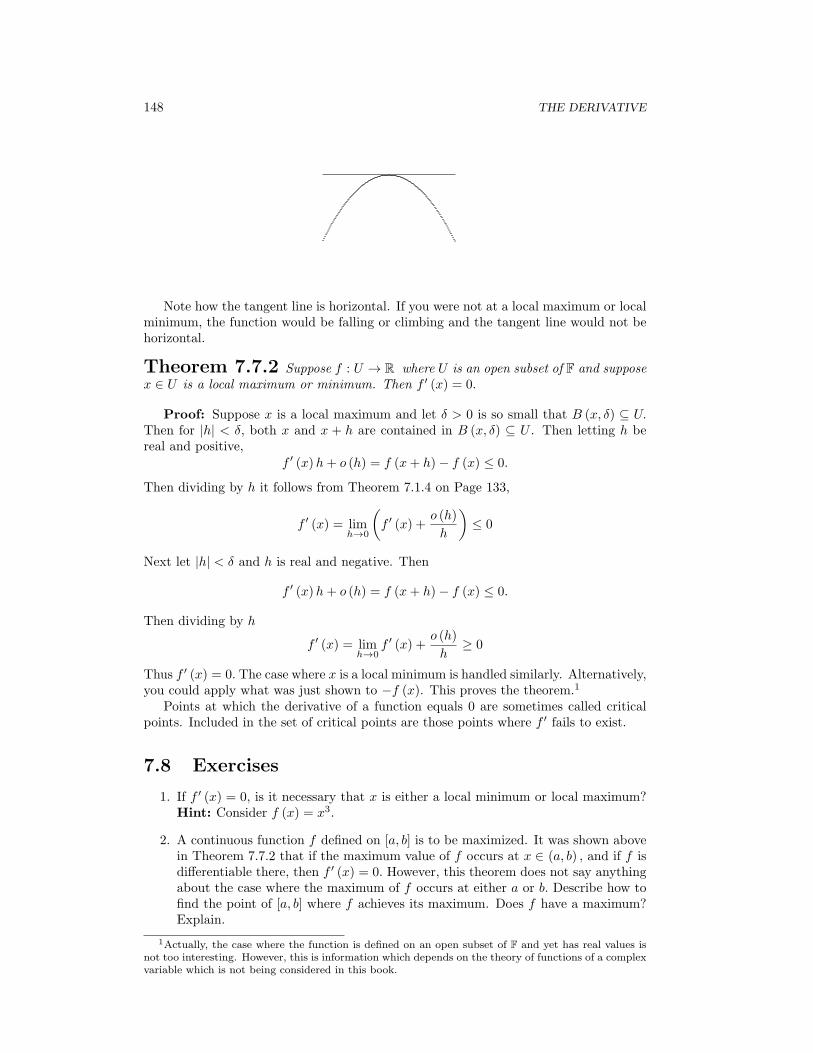
148 THE DERIVATIVE
Note how the tangent line is horizontal. If you were not at a local maximum or localminimum, the function would be falling or climbing and the tangent line would not behorizontal.
Theorem 7.7.2 Suppose f : U → R where U is an open subset of F and supposex ∈ U is a local maximum or minimum. Then f ′ (x) = 0.
Proof: Suppose x is a local maximum and let δ > 0 is so small that B (x, δ) ⊆ U.Then for |h| < δ, both x and x + h are contained in B (x, δ) ⊆ U . Then letting h bereal and positive,
f ′ (x)h+ o (h) = f (x+ h)− f (x) ≤ 0.
Then dividing by h it follows from Theorem 7.1.4 on Page 133,
f ′ (x) = limh→0
(f ′ (x) +
o (h)
h
)≤ 0
Next let |h| < δ and h is real and negative. Then
f ′ (x)h+ o (h) = f (x+ h)− f (x) ≤ 0.
Then dividing by h
f ′ (x) = limh→0
f ′ (x) +o (h)
h≥ 0
Thus f ′ (x) = 0. The case where x is a local minimum is handled similarly. Alternatively,you could apply what was just shown to −f (x). This proves the theorem.1
Points at which the derivative of a function equals 0 are sometimes called criticalpoints. Included in the set of critical points are those points where f ′ fails to exist.
7.8 Exercises
1. If f ′ (x) = 0, is it necessary that x is either a local minimum or local maximum?Hint: Consider f (x) = x3.
2. A continuous function f defined on [a, b] is to be maximized. It was shown abovein Theorem 7.7.2 that if the maximum value of f occurs at x ∈ (a, b) , and if f isdifferentiable there, then f ′ (x) = 0. However, this theorem does not say anythingabout the case where the maximum of f occurs at either a or b. Describe how tofind the point of [a, b] where f achieves its maximum. Does f have a maximum?Explain.
1Actually, the case where the function is defined on an open subset of F and yet has real values isnot too interesting. However, this is information which depends on the theory of functions of a complexvariable which is not being considered in this book.
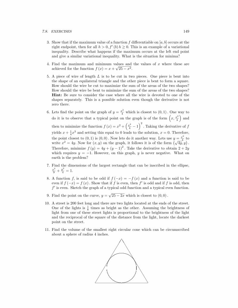
7.8. EXERCISES 149
3. Show that if the maximum value of a function f differentiable on [a, b] occurs at theright endpoint, then for all h > 0, f ′ (b)h ≥ 0. This is an example of a variationalinequality. Describe what happens if the maximum occurs at the left end pointand give a similar variational inequality. What is the situation for minima?
4. Find the maximum and minimum values and the values of x where these areachieved for the function f (x) = x+
√25− x2.
5. A piece of wire of length L is to be cut in two pieces. One piece is bent intothe shape of an equilateral triangle and the other piece is bent to form a square.How should the wire be cut to maximize the sum of the areas of the two shapes?How should the wire be bent to minimize the sum of the areas of the two shapes?Hint: Be sure to consider the case where all the wire is devoted to one of theshapes separately. This is a possible solution even though the derivative is notzero there.
6. Lets find the point on the graph of y = x2
4 which is closest to (0, 1) . One way to
do it is to observe that a typical point on the graph is of the form(x, x
2
4
)and
then to minimize the function f (x) = x2 +(
x2
4 − 1)2. Taking the derivative of f
yields x+ 14x
3 and setting this equal to 0 leads to the solution, x = 0. Therefore,
the point closest to (0, 1) is (0, 0) . Now lets do it another way. Lets use y = x2
4 towrite x2 = 4y. Now for (x, y) on the graph, it follows it is of the form
(√4y, y
).
Therefore, minimize f (y) = 4y + (y − 1)2. Take the derivative to obtain 2 + 2y
which requires y = −1. However, on this graph, y is never negative. What onearth is the problem?
7. Find the dimensions of the largest rectangle that can be inscribed in the ellipse,x2
9 + y2
4 = 1.
8. A function f, is said to be odd if f (−x) = −f (x) and a function is said to beeven if f (−x) = f (x) . Show that if f is even, then f ′ is odd and if f is odd, thenf ′ is even. Sketch the graph of a typical odd function and a typical even function.
9. Find the point on the curve, y =√25− 2x which is closest to (0, 0) .
10. A street is 200 feet long and there are two lights located at the ends of the street.One of the lights is 1
8 times as bright as the other. Assuming the brightness oflight from one of these street lights is proportional to the brightness of the lightand the reciprocal of the square of the distance from the light, locate the darkestpoint on the street.
11. Find the volume of the smallest right circular cone which can be circumscribedabout a sphere of radius 4 inches.
������������
TT
TT
TT
TT
TT
TT

150 THE DERIVATIVE
12. Show that for r a rational number and y = xr, it must be the case that if thisfunction is differentiable, then y′ = rxr−1.
13. Let f be a continuous function defined on [a, b] . Let ε > 0 be given. Show thereexists a polynomial, p such that for all x ∈ [a, b] ,
|f (x)− p (x)| < ε.
This follows from the Weierstrass approximation theorem, Theorem 6.12.3. Nowhere is the interesting part. Show there exists a function g which is also continuouson [a, b] and for all x ∈ [a, b] ,
|f (x)− g (x)| < ε
but g has no derivative at any point. Thus there are enough nowhere differentiablefunctions that any continuous function is uniformly close to one. Explain whyevery continuous function is the uniform limit of nowhere differentiable functions.Also explain why every nowhere differentiable continuous function is the uniformlimit of polynomials. Hint: You should look at the construction of the nowheredifferentiable function which is everywhere continuous, given above.
14. Consider the following nested sequence of compact sets, {Pn}. Let P1 = [0, 1],P2 =
[0, 13
]∪[23 , 1], etc. To go from Pn to Pn+1, delete the open interval which
is the middle third of each closed interval in Pn. Let P = ∩∞n=1Pn. By Problem13 on Page 62, P = ∅. If you have not worked this exercise, now is the time to doit. Show the total length of intervals removed from [0, 1] is equal to 1. If you feelambitious also show there is a one to one onto mapping of [0, 1] to P . The set Pis called the Cantor set. Thus P has the same number of points in it as [0, 1] inthe sense that there is a one to one and onto mapping from one to the other eventhough the length of the intervals removed equals 1. Hint: There are variousways of doing this last part but the most enlightenment is obtained by exploitingthe construction of the Cantor set rather than some silly representation in termsof sums of powers of two and three. All you need to do is use the theorems in thechapter on set theory related to the Schroder Bernstein theorem and show thereis an onto map from the Cantor set to [0, 1]. If you do this right it will providea construction which is very useful to prove some even more surprising theoremswhich you may encounter later if you study compact metric spaces.
15. ↑ Consider the sequence of functions defined in the following way. Let f1 (x) = x on[0, 1]. To get from fn to fn+1, let fn+1 = fn on all intervals where fn is constant. Iffn is nonconstant on [a, b], let fn+1(a) = fn(a), fn+1(b) = fn(b), fn+1 is piecewiselinear and equal to 1
2 (fn(a) + fn(b)) on the middle third of [a, b]. Sketch a fewof these and you will see the pattern. The process of modifying a nonconstantsection of the graph of this function is illustrated in the following picture.
���
Show {fn} converges uniformly on [0, 1]. If f(x) = limn→∞ fn(x), show thatf(0) = 0, f(1) = 1, f is continuous, and f ′(x) = 0 for all x /∈ P where P isthe Cantor set of Problem 14. This function is called the Cantor function.It is avery important example to remember especially for those who like mathematicalpathology. Note it has derivative equal to zero on all those intervals which wereremoved and whose total length was equal to 1 and yet it succeeds in climbing

7.9. WORKED EXERCISES 151
from 0 to 1. Isn’t this amazing? Hint: This isn’t too hard if you focus on gettinga careful estimate on the difference between two successive functions in the listconsidering only a typical small interval in which the change takes place. Theabove picture should be helpful.
16. Let
f (x) =
{1 if x ∈ Q0 if x /∈ Q
Now let g (x) = x2f (x) . Find where g is continuous and differentiable if anywhere.
7.9 Worked Exercises
1. Show that if the maximum value of a function f differentiable on [a, b] occurs at theright endpoint, then for all h > 0, f ′ (b)h ≥ 0. This is an example of a variationalinequality. Describe what happens if the maximum occurs at the left end pointand give a similar variational inequality. What is the situation for minima?
By assumption, if h > 0,
f (b+ (−th))− f (b)− f ′ (b) (−th) = o (th)
and sof ′ (b) th = f (b)− f (b+ (−th)) + o (t) ≥ o (t)
Now divide by t > 0 and let t→ 0.
2. A function f, is said to be odd if f (−x) = −f (x) and a function is said to beeven if f (−x) = f (x) . Show that if f is even, then f ′ is odd and if f is odd, thenf ′ is even. Sketch the graph of a typical odd function and a typical even function.
Suppose f is even. Then f (−x) = f (x) and using the chain rule on both sides,f ′ (−x) (−1) = f ′ (x) and so f ′ is odd. The other case is similar.
3. Let f be a continuous function defined on [a, b] . Let ε > 0 be given. Show thereexists a polynomial, p such that for all x ∈ [a, b] ,
|f (x)− p (x)| < ε.
This follows from the Weierstrass approximation theorem, Theorem 6.12.3. Nowhere is the interesting part. Show there exists a function g which is also continuouson [a, b] and for all x ∈ [a, b] ,
|f (x)− g (x)| < ε
but g has no derivative at any point. Thus there are enough nowhere differentiablefunctions that any continuous function is uniformly close to one. Explain whyevery continuous function is the uniform limit of nowhere differentiable functions.Also explain why every nowhere differentiable continuous function is the uniformlimit of polynomials. Hint: You should look at the construction of the nowheredifferentiable function which is everywhere continuous, given above.
Take that bounded nowhere differentiable function g which was bounded by 2 inabsolute value and form f (x) + δg (x) where δ is very small, smaller than ε/2.
4. Consider the following nested sequence of compact sets, {Pn}. Let P1 = [0, 1],P2 =
[0, 13
]∪[23 , 1], etc. To go from Pn to Pn+1, delete the open interval which
is the middle third of each closed interval in Pn. Let P = ∩∞n=1Pn. By Problem

152 THE DERIVATIVE
13 on Page 62, P = ∅. If you have not worked this exercise, now is the time to doit. Show the total length of intervals removed from [0, 1] is equal to 1. If you feelambitious also show there is a one to one onto mapping of [0, 1] to P . The set Pis called the Cantor set. Thus P has the same number of points in it as [0, 1] inthe sense that there is a one to one and onto mapping from one to the other eventhough the length of the intervals removed equals 1. Hint: There are variousways of doing this last part but the most enlightenment is obtained by exploitingthe construction of the Cantor set rather than some silly representation in termsof sums of powers of two and three. All you need to do is use the theorems in thechapter on set theory related to the Schroder Bernstein theorem and show thereis an onto map from the Cantor set to [0, 1]. If you do this right it will providea construction which is very useful to prove some even more surprising theoremswhich you may encounter later if you study compact metric spaces.
That P is nonempty follows from it being the intersection of a nested sequence ofsequentially compact sets. What is the length of the set removed?
1
3+
2
32+
4
33+ · · · =
∞∑k=1
2k−1
3k= 1
Next consider the claim about the one to one onto mapping of [0, 1] to P . Let the
2n intervals in Pn be denoted by {Ik}2n
k=1 . Each of these intervals is of length 3−n.
Let the closed intervals {Jnk }
2n
k=1 be obtained by simply bisecting the intervals eachtime without taking out the middle third. Then a point x ∈ P is and only if itis in a sequence
{Inkn
}of the intervals used in the construction of the Cantor set.
Define f (x) ≡ ∩∞n=1Jnkn
where Jnk corresponds to Ink in the sense they are both
the kth interval from the left. Then since the diameters of the Jnkn
converge to 0,this specifies a unique point. Thus f : P → [0, 1] is clearly onto because given apoint of [0, 1] you can get a sequence
{Jnkn
}each of which contains x. Therefore,
the construction yields a point of P which f maps to x. There is obviously anonto mapping from [0, 1] to P and so by the material on set theory, there existsa one to one and onto mapping from P to [0, 1].
5. ↑ Consider the sequence of functions defined in the following way. Let f1 (x) = x on[0, 1]. To get from fn to fn+1, let fn+1 = fn on all intervals where fn is constant. Iffn is nonconstant on [a, b], let fn+1(a) = fn(a), fn+1(b) = fn(b), fn+1 is piecewiselinear and equal to 1
2 (fn(a) + fn(b)) on the middle third of [a, b]. Sketch a fewof these and you will see the pattern. The process of modifying a nonconstantsection of the graph of this function is illustrated in the following picture.
���
Show {fn} converges uniformly on [0, 1]. If f(x) = limn→∞ fn(x), show thatf(0) = 0, f(1) = 1, f is continuous, and f ′(x) = 0 for all x /∈ P where P isthe Cantor set of Problem 14. This function is called the Cantor function.It is avery important example to remember especially for those who like mathematicalpathology. Note it has derivative equal to zero on all those intervals which wereremoved and whose total length was equal to 1 and yet it succeeds in climbingfrom 0 to 1. Isn’t this amazing? Hint: This isn’t too hard if you focus on gettinga careful estimate on the difference between two successive functions in the listconsidering only a typical small interval in which the change takes place. Theabove picture should be helpful.

7.10. MEAN VALUE THEOREM 153
From the picture, the maximum distance between fn and fn+1 is 2−n − 3−n. Itfollows
limn→∞
fn+1 (x) = f1 (x) +n∑
k=1
fk+1 (x)− fk (x)
and this converges uniformly by the Weierstrass M test. Let Mk = 2−n − 3−n. Itfollows f is continuous, f ′ (x) = 0 off P and yet it climbs from 0 to 1. Note thatthis function also gives a mapping of P onto [0, 1]. (Why?)
7.10 Mean Value Theorem
The mean value theorem is possibly the most important theorem about the derivativeof a function of one variable. It pertains only to a real valued function of a real variable.The best versions of many other theorems depend on this fundamental result. The meanvalue theorem is based on the following special case known as Rolle’s theorem2. It is anexistence theorem and like the other existence theorems in analysis, it depends on thecompleteness axiom.
Theorem 7.10.1 Suppose f : [a, b]→ R is continuous,
f (a) = f (b) ,
andf : (a, b)→ R
has a derivative at every point of (a, b) . Then there exists x ∈ (a, b) such that f ′ (x) =0.
Proof: Suppose first that f (x) = f (a) for all x ∈ [a, b] . Then any x ∈ (a, b) is apoint such that f ′ (x) = 0. If f is not constant, either there exists y ∈ (a, b) such thatf (y) > f (a) or there exists y ∈ (a, b) such that f (y) < f (b) . In the first case, themaximum of f is achieved at some x ∈ (a, b) and in the second case, the minimum off is achieved at some x ∈ (a, b). Either way, Theorem 7.7.2 implies f ′ (x) = 0. Thisproves Rolle’s theorem.
The next theorem is known as the Cauchy mean value theorem. It is the best versionof this important theorem.
Theorem 7.10.2 Suppose f, g are continuous on [a, b] and differentiable on(a, b) . Then there exists x ∈ (a, b) such that
f ′ (x) (g (b)− g (a)) = g′ (x) (f (b)− f (a)) .
Proof:Leth (x) ≡ f (x) (g (b)− g (a))− g (x) (f (b)− f (a)) .
Then letting x = a and then letting x = b, a short computation shows h (a) = h (b) .Also, h is continuous on [a, b] and differentiable on (a, b) . Therefore Rolle’s theoremapplies and there exists x ∈ (a, b) such that
h′ (x) = f ′ (x) (g (b)− g (a))− g′ (x) (f (b)− f (a)) = 0.
This proves the theorem.
2Rolle is remembered for Rolle’s theorem and not for anything else he did. Ironically, he did notlike calculus.

154 THE DERIVATIVE
Letting g (x) = x, the usual version of the mean value theorem is obtained. Here isthe usual picture which describes the theorem.
���������
��������
a b
Corollary 7.10.3 Let f be a continuous real valued function defined on [a, b] anddifferentiable on (a, b) . Then there exists x ∈ (a, b) such that f (b)−f (a) = f ′ (x) (b− a) .
Corollary 7.10.4 Suppose f ′ (x) = 0 for all x ∈ (a, b) where a ≥ −∞ and b ≤ ∞.Then f (x) = f (y) for all x, y ∈ (a, b) . Thus f is a constant.
Proof: If this is not true, there exists x1 and x2 such that f (x1) = f (x2) . Thenby the mean value theorem,
0 = f (x1)− f (x2)x1 − x2
= f ′ (z)
for some z between x1 and x2. This contradicts the hypothesis that f ′ (x) = 0 for all x.This proves the theorem in the case that f has real values. In the general case,
f (x+ h)− f (x)− 0h = o (h) .
Then taking the real part of both sides,
Re f (x+ h)− Re f (x) = Re o (h) = o (h)
and so Re f ′ (x) = 0 and by the first part, Re f must be a constant. The same reasoningapplies to Im f and this proves the corollary.
Corollary 7.10.5 Suppose f : C→ C and f ′ (x) = 0 for all x. Then f is a constant.
Proof: Let t ∈ R and consider h (t) = f (x+ t (y − x))− f (x) . Then by the chainrule,
h′ (t) = f ′ (x+ t (y − x)) (y − x) = 0
and so by Corollary 7.10.4 h is a constant. In particular,
h (1) = f (y)− f (x) = h (0) = 0
which shows f is constant since x, y are arbitrary. This proves the corollary.
Corollary 7.10.6 Suppose f ′ (x) > 0 for all x ∈ (a, b) where a ≥ −∞ and b ≤ ∞.Then f is strictly increasing on (a, b) . That is, if x < y, then f (x) < f (y) . If f ′ (x) ≥ 0,then f is increasing in the sense that whenever x < y it follows that f (x) ≤ f (y) .
Proof: Let x < y. Then by the mean value theorem, there exists z ∈ (x, y) suchthat
0 < f ′ (z) =f (y)− f (x)
y − x.
Since y > x, it follows f (y) > f (x) as claimed. Replacing < by ≤ in the above equationand repeating the argument gives the second claim.
7.11. EXERCISES 155
Corollary 7.10.7 Suppose f ′ (x) < 0 for all x ∈ (a, b) where a ≥ −∞ and b ≤ ∞.Then f is strictly decreasing on (a, b) . That is, if x < y, then f (x) > f (y) . If f ′ (x) ≤ 0,then f is decreasing in the sense that for x < y, it follows that f (x) ≥ f (y)
Proof: Let x < y. Then by the mean value theorem, there exists z ∈ (x, y) suchthat
0 > f ′ (z) =f (y)− f (x)
y − x.
Since y > x, it follows f (y) < f (x) as claimed. The second claim is similar exceptinstead of a strict inequality in the above formula, you put ≥ .
7.11 Exercises
1. Sally drives her Saturn over the 110 mile toll road in exactly 1.3 hours. The speedlimit on this toll road is 70 miles per hour and the fine for speeding is 10 dollarsper mile per hour over the speed limit. How much should Sally pay?
2. Two cars are careening down a freeway weaving in and out of traffic. Car Apasses car B and then car B passes car A as the driver makes obscene gestures.This infuriates the driver of car A who passes car B while firing his handgun atthe driver of car B. Show there are at least two times when both cars have thesame speed. Then show there exists at least one time when they have the sameacceleration. The acceleration is the derivative of the velocity.
3. Show the cubic function f (x) = 5x3 + 7x− 18 has only one real zero.
4. Suppose f (x) = x7 + |x|+ x− 12. How many solutions are there to the equation,f (x) = 0?
5. Let f (x) = |x− 7| + (x− 7)2 − 2 on the interval [6, 8] . Then f (6) = 0 = f (8) .
Does it follow from Rolle’s theorem that there exists c ∈ (6, 8) such that f ′ (c) = 0?Explain your answer.
6. Suppose f and g are differentiable functions defined on R. Suppose also that itis known that |f ′ (x)| > |g′ (x)| for all x and that |f ′ (t)| > 0 for all t. Show thatwhenever x = y, it follows |f (x)− f (y)| > |g (x)− g (y)| . Hint: Use the Cauchymean value theorem, Theorem 7.10.2.
7. Show that, like continuous functions, functions which are derivatives have theintermediate value property. This means that if f ′ (a) < 0 < f ′ (b) then thereexists x ∈ (a, b) such that f ′ (x) = 0. Hint: Argue the minimum value of f occursat an interior point of [a, b] .
8. Find an example of a function which has a derivative at every point but such thatthe derivative is not everywhere continuous.
9. Consider the function
f (x) ≡{
1 if x ≥ 0−1 if x < 0
.
Is it possible that this function could be the derivative of some function? Why?
10. Suppose a ∈ I, an open interval and that a function f, defined on I has n + 1derivatives. Then for each m ≤ n the following formula holds for x ∈ I.
f (x) =
m∑k=0
f (k) (a)(x− a)k
k!+ f (m+1) (y)
(x− a)m+1
(m+ 1)!(7.17)

156 THE DERIVATIVE
where y is some point between x and a. Note that if n = 0, this reduces to theLagrange form of the mean value theorem, so the formula holds if m = 0. Supposeit holds for some 0 ≤ m < n. The task is to show then that it also holds for m+1.It will then follow that the above formula will hold for all m ≤ n as claimed.This formula is very important. The last term is called the Lagrange form of theremainder in Taylor series. Try to prove the formula using the following steps. Ifthe formula holds for every function having m derivatives, then if f has m + 1derivatives, you can write the formula for its derivative, a function which has mderivatives. Thus, you obtain
f ′ (x)−m−1∑k=0
(f ′)(k)
(a)
k!(x− a)k =
(f ′)(m)
(y)
m!(x− a)m
Thus
f ′ (x)−m−1∑k=0
f (k+1) (a)
k!(x− a)k =
f (m+1) (y)
m!(x− a)m . (7.18)
Now let g (x) = f (x) −∑m
k=0f(k)(a)
k! (x− a)k and let h (x) = (x− a)m+1. From
the Cauchy mean value theorem, there exists z between x and a such that
g (x)− g (a)h (x)− h (a)
=g′ (z)
h′ (z)=f ′ (z)−
∑mk=1
f(k)(a)(k−1)! (z − a)
k−1
(m+ 1) (z − a)m.
Now explain why∑m
k=1f(k)(a)(k−1)! (z − a)
k−1=∑m−1
k=0f(k+1)(a)
k! (z − a)k and then use
7.18. Explain why this implies
f (x)−∑m
k=0f(k)(a)
k! (x− a)k
(x− a)m+1 =f(m+1)(y)
m! (z − a)m
(m+ 1) (z − a)m
which yields the desired formula for m. A way to think of 7.17 is as a generalizedmean value theorem. Note that the key result which made it work was the Cauchymean value theorem.
11. Now here is another way to obtain the above approximation. Fix c, x in (a, b) aninterval on which f has n+ 1 derivatives. Let K be a number, depending on c, xsuch that
f (x)−
(f (c) +
n∑k=1
f (k) (c)
k!(x− c)k +K (x− c)n+1
)= 0
Now the idea is to find K. To do this, let
F (t) = f (x)−
(f (t) +
n∑k=1
f (k) (t)
k!(x− t)k +K (x− t)n+1
)
Then F (x) = F (c) = 0. Therefore, by Rolle’s theorem there exists z between aand x such that F ′ (z) = 0. Do the differentiation and solve for K.
12. Let f be a real continuous function defined on the interval [0, 1] . Also supposef (0) = 0 and f (1) = 1 and f ′ (t) exists for all t ∈ (0, 1) . Show there exists ndistinct points {si}ni=1 of the interval such that
n∑i=1
f ′ (si) = n.
7.12. WORKED EXERCISES 157
Hint: Consider the mean value theorem applied to successive pairs in the followingsum.
f
(1
3
)− f (0) + f
(2
3
)− f
(1
3
)+ f (1)− f
(2
3
)13. Now suppose f : [0, 1]→ R and f (0) = 0 while f (1) = 1. Show there are distinct
points {si}ni=1 ⊆ (0, 1) such that
n∑i=1
(f ′ (si))−1
= n.
Hint: Let 0 = t0 < t1 < · · · < tn = 1 and pick xi ∈ f−1 (ti) such that these xiare increasing and xn = 1, x0 = 0. Explain why you can do this. Then argue
ti+1 − ti = f (xi+1)− f (xi) = f ′ (si) (xi+1 − xi)
and soxi+1 − xiti+1 − ti
=1
f ′ (si)
Now choose the ti to be equally spaced.
7.12 Worked Exercises
1. Sally drives her Saturn over the 110 mile toll road in exactly 1.3 hours. The speedlimit on this toll road is 70 miles per hour and the fine for speeding is 10 dollarsper mile per hour over the speed limit. How much should Sally pay?
Her average speed is 1101.3 = 84. 615 384 6 and so she did achieve at least this speed
at some time by the mean value theorem. She should pay at least $140.
2. Suppose f and g are differentiable functions defined on R. Suppose also that itis known that |f ′ (x)| > |g′ (x)| for all x and that |f ′ (t)| > 0 for all t. Show thatwhenever x = y, it follows |f (x)− f (y)| > |g (x)− g (y)| . Hint: Use the Cauchymean value theorem, Theorem 7.10.2.
The Cauchy mean value theorem says there exists t between y and x such that
f ′ (t) (g (x)− g (y)) = g′ (t) (f (x)− f (y))
Therefore,|f ′ (t)| |g (x)− g (y)| = |g′ (t)| |f (x)− f (y)|
Now suppose for some x, y, |f (x)− f (y)| ≤ |g (x)− g (y)| . Then from the above,
|f ′ (t)| |f (x)− f (y)| ≤ |g′ (t)| |f (x)− f (y)|
Now |f (x)− f (y)| = 0 because this would contradict the mean value theoremand |f ′ (x)| = 0. Therefore, this would require |f ′ (t)| ≤ |g′ (t)| which contradictsthe assumption.
3. Show that, like continuous functions, functions which are derivatives have theintermediate value property. This means that if f ′ (a) < 0 < f ′ (b) then thereexists x ∈ (a, b) such that f ′ (x) = 0. Hint: Argue the minimum value of f occursat an interior point of [a, b] .
The assumption requires the minimum of f to occur at an interior point because,for example
f (x)− f (b)− f ′ (b) (x− b) = o (x− b)

158 THE DERIVATIVE
f (x)− f (b) = f ′ (b) (x− b) + o (x− b)
and so if 0 < |x− b| is small enough, |o (x− b)| < f ′(b)2 |x− b|. Thus for x close
enough to b,
f (x)− f (b) < −f ′ (b) |x− b|+ f ′ (b)
2|x− b| < 0
and so the minimum does not occur at b. Similar reasoning shows the minimumof f does not occur at a. Therefore, there exists x ∈ (a, b) such that f ′ (x) = 0.
4. Find an example of a function which has a derivative at every point but such thatthe derivative is not everywhere continuous.
f (x) = x2 sin(1x
)for x = 0 and f (0) ≡ 0. This one works.
5. Now suppose f : [0, 1]→ R and f (0) = 0 while f (1) = 1. Show there are distinctpoints {si}ni=1 ⊆ (0, 1) such that
n∑i=1
(f ′ (si))−1
= n.
Hint: Let 0 = t0 < t1 < · · · < tn = 1 and pick xi ∈ f−1 (ti) such that these xiare increasing and xn = 1, x0 = 0. Explain why you can do this. Then argue
ti+1 − ti = f (xi+1)− f (xi) = f ′ (si) (xi+1 − xi)
and soxi+1 − xiti+1 − ti
=1
f ′ (si)
Now choose the ti to be equally spaced.
In finding the xi, let xi be the smallest in f−1 (ti) , i < n but let xn = 1. Thenthe smallest in f−1 (ti+1) must be larger than xi because if it were smaller, thenby intermediate value theorem, xi was not really the smallest in f−1 (ti). Lettingti+1 − ti = 1/n, the hint yields the desired result.
n = n∑i
(xi+1 − xi) =∑i
1
f ′ (si)
7.13 Derivatives Of Inverse Functions
It happens that if f is a differentiable one to one function defined on an interval, [a, b] ,and f ′ (x) exists and is non zero then the inverse function f−1 has a derivative at thepoint f (x) . Recall that f−1 is defined according to the formula
f−1 (f (x)) = x.
Let f : [a, b]→ R be a continuous function. Recall from Theorem 7.6.1
f ′ (a) ≡ limx→a+
f (x)− f (a)x− a
, f ′ (b) ≡ limx→b−
f (x)− f (b)x− b
.
Recall the notation x→ a+ means that only x > a are considered in the definitionof limit, the notation x → b− defined similarly. Thus, this definition includes thederivative of f at the endpoints of the interval and to save notation,
f ′ (x1) ≡ limx→x1
f (x)− f (x1)x− x1
where it is understood that x is always in [a, b] .
7.13. DERIVATIVES OF INVERSE FUNCTIONS 159
Theorem 7.13.1 Let f : [a, b] → R be continuous and one to one. Suppose
f ′ (x1) exists for some x1 ∈ [a, b] and f ′ (x1) = 0. Then(f−1
)′(f (x1)) exists and is
given by the formula,(f−1
)′(f (x1)) =
1f ′(x1)
.
Proof:By Lemma 6.5.3, and Corollary 6.5.4 on Page 115 f is either strictly increas-ing or strictly decreasing and f−1 is continuous. Therefore there exists η > 0 such thatif 0 < |f (x1)− f (x)| < η, then
0 < |x1 − x| =∣∣f−1 (f (x1))− f−1 (f (x))
∣∣ < δ
where δ is small enough that for 0 < |x1 − x| < δ,∣∣∣∣ x− x1f (x)− f (x1)
− 1
f ′ (x1)
∣∣∣∣ < ε.
It follows that if 0 < |f (x1)− f (x)| < η,∣∣∣∣f−1 (f (x))− f−1 (f (x1))
f (x)− f (x1)− 1
f ′ (x1)
∣∣∣∣ = ∣∣∣∣ x− x1f (x)− f (x1)
− 1
f ′ (x1)
∣∣∣∣ < ε
Therefore, since ε > 0 is arbitrary,
limy→f(x1)
f−1 (y)− f−1 (f (x1))
y − f (x1)=
1
f ′ (x1)
and this proves the theorem.
The following obvious corollary comes from the above by not bothering with endpoints.
Corollary 7.13.2 Let f : (a, b) → R, where −∞ ≤ a < b ≤ ∞ be continuousand one to one. Suppose f ′ (x1) exists for some x1 ∈ (a, b) and f ′ (x1) = 0. Then(f−1
)′(f (x1)) exists and is given by the formula,
(f−1
)′(f (x1)) =
1f ′(x1)
.
This is one of those theorems which is very easy to remember if you neglect thedifficult questions and simply focus on formal manipulations. Consider the following.
f−1 (f (x)) = x.
Now use the chain rule on both sides to write(f−1
)′(f (x)) f ′ (x) = 1,
and then divide both sides by f ′ (x) to obtain
(f−1
)′(f (x)) =
1
f ′ (x).
Of course this gives the conclusion of the above theorem rather effortlessly and it isformal manipulations like this which aid in remembering formulas such as the one givenin the theorem.
Example 7.13.3 Let f (x) = 1 + x2 + x3 + 7. Show that f has an inverse and find(f−1
)′(8) .

160 THE DERIVATIVE
I am not able to find a formula for the inverse function. This is typical in usefulapplications so you need to get used to this idea. The methods of algebra are insufficientto solve hard problems in analysis. You need something more. The question is todetermine whether f has an inverse. To do this,
f ′ (x) = 2x+ 3x2 + 7 > 0
By Corollary 7.10.6 on Page 154, this function is strictly increasing on R and so it has aninverse function although I have no idea how to find an explicit formula for this inversefunction. However, I can see that f (0) = 8 and so by the formula for the derivative ofan inverse function, (
f−1)′(8) =
(f−1
)′(f (0)) =
1
f ′ (0)=
1
7.
7.14 Derivatives And Limits Of Sequences
When you have a function which is a limit of a sequence of functions, when can yousay the derivative of the limit function is the limit of the derivatives of the functions inthe sequence? The following theorem seems to be one of the best results available. Itis based on the mean value theorem. First of all, recall Definition 6.11.5 on Page 121listed here for convenience.
Definition 7.14.1 Let {fn} be a sequence of functions defined on D. Then {fn}is said to converge uniformly to f if it converges pointwise to f and for every ε > 0there exists N such that for all n ≥ N
|f (x)− fn (x)| < ε
for all x ∈ D.
To save on notation, denote by
||k|| ≡ sup {|k (ξ)| : ξ ∈ D} .
Then||k + l|| ≤ ||k||+ ||l|| (7.19)
because for each ξ ∈ D,|k (ξ) + l (ξ)| ≤ ||k||+ ||l||
and taking sup yields 7.19. From the definition of uniform convergence, you see that fnconverges uniformly to f is the same as saying
limn→∞
||fn − f || = 0.
Now here is the theorem.
Theorem 7.14.2 Let (a, b) be a finite open interval and let fk : (a, b) → R bedifferentiable and suppose there exists x0 ∈ (a, b) such that
{fk (x0)} converges,
{f ′k} converges uniformly to a function g on (a, b) .
Then there exists a function f defined on (a, b) such that
fk → f uniformly,
andf ′ = g.
7.15. EXERCISES 161
Proof: Let c ∈ (a, b) and define
gn (x, c) ≡{
fn(x)−fn(c)x−c if x = c
f ′n (c) if x = c.
Also let||h|| ≡ sup {|h (x)| : x ∈ (a, b)} .
Thus hk → h uniformly means ||hk − h|| → 0.Claim 1: For each c, x → gn (x, c) converges uniformly to a continuous function
hc, on (a, b) .Proof: First note that each x → gn (x, c) is continuous. Next consider the claim
about uniform convergence. Let x = c. Then by the mean value theorem applied to thefunction x→ fn (x)− fm (x),
|gn (x, c)− gm (x, c)|
=
∣∣∣∣fn (x)− fm (x)− (fn (c)− fm (c))
x− c
∣∣∣∣= |f ′n (ξ)− f ′m (ξ)| ≤ |f ′n (ξ)− g (ξ)|+ |g (ξ)− f ′m (ξ)|≤ ||f ′n − g||+ ||f ′m − g||
By the assumption that {f ′n} converges uniformly to g, it follows each of the last twoterms converges to 0 as n, m→∞. If x = c, then
|gn (c, c)− gm (c, c)| = |f ′n (c)− f ′m (c)| ≤ ||f ′n − g||+ ||f ′m − g||
Thus x → gn (x, c) is uniformly Cauchy and must converge uniformly to a continuousfunction hc by Theorem 6.11.6 and Corollary 6.11.9. This proves the first claim.
Claim 2: fn converges uniformly to a function f.Proof: From the definition of gn in the case where c = x0,
fn (x)− fn (x0) = gn (x, x0) (x− x0) . (7.20)
Hence from the above claim, fn converges uniformly because it is given that fn (x0)converges to f (x0).
Now to complete the proof of the theorem, for c given and x = c,
f (x)− f (c)x− c
= limn→∞
fn (x)− fn (c)x− c
= limn→∞
gn (x, c) = hc (x) .
Since hc is continuous,
limx→c
f (x)− f (c)x− c
= limx→c
hc (x) = hc (c) .
It remains to verify hc (c) = g (c) . This is easy because gn (c, c) ≡ f ′n (c) → g (c) andgn (c, c)→ hc (c) . This proves the theorem.
7.15 Exercises
1. It was shown earlier that the nth root of a positive number exists whenever n is apositive integer. Let y = x1/n. Prove y′ (x) = 1
nx(1/n)−1.
2. Now for positive x and p, q positive integers, y = xp/q is defined by y = q√xp. Find
and prove a formula for dy/dx.

162 THE DERIVATIVE
3. For 1 ≥ x ≥ 0, and p ≥ 1, show that (1− x)p ≥ 1− px. Hint: This can be doneusing the mean value theorem. Define f (x) ≡ (1− x)p − 1 + px and show thatf (0) = 0 while f ′ (x) ≥ 0 for all x ∈ (0, 1) .
4. Using the result of Problem 3 establish Raabe’s Test, an interesting variation onthe ratio test. This test says the following. Suppose there exists a constant, Cand a number p such that ∣∣∣∣ak+1
ak
∣∣∣∣ ≤ 1− p
k + C
for all k large enough. Then if p > 1, it follows that∑∞
k=1 ak converges absolutely.Hint: Let bk ≡ k−1+C and note that for all k large enough, bk > 1. Now concludethat there exists an integer, k0 such that bk0 > 1 and for all k ≥ k0 the giveninequality above holds. Use Problem 3 to conclude that∣∣∣∣ak+1
ak
∣∣∣∣ ≤ 1− p
k + C≤(1− 1
k + C
)p
=
(bkbk+1
)p
showing that |ak| bpk is decreasing for k ≥ k0. Thus |ak| ≤ C/bpk = C/ (k − 1 + C)p.
Now use comparison theorems and the p series to obtain the conclusion of thetheorem.
5. The graph of a function y = f (x) is said to be concave up or more simply “convex”if whenever (x1, y1) and (x2, y2) are two points such that yi ≥ f (xi) , it follows thatfor each point, (x, y) on the straight line segment joining (x1, y1) and (x2, y2) , y ≥f (x) . Show that if f is twice differentiable on an open interval, (a, b) and f ′′ (x) >0, then the graph of f is convex.
6. Show that if the graph of a function f defined on an interval (a, b) is convex, thenif f ′ exists on (a, b) , it must be the case that f ′ is an increasing function. Noteyou do not know the second derivative exists.
7. Convex functions defined in Problem 5 have a very interesting property. Suppose{ai}ni=1 are all nonnegative, sum to 1, and suppose ϕ is a convex function definedon R. Then
ϕ
(n∑
k=1
akxk
)≤
n∑k=1
akϕ (xk) .
Verify this interesting inequality.
8. If ϕ is a convex function defined on R, show that ϕ must be continuous at everypoint.
9. Prove the second derivative test. If f ′ (x) = 0 at x ∈ (a, b) , an interval on whichf is defined and both f ′, f ′′ exist and are continuous on this interval, then iff ′′ (x) > 0, it follows f has a local minimum at x and if f ′′ (x) < 0, then f has alocal maximum at x. Show that if f ′′ (x) = 0 no conclusion about the nature ofthe critical point can be drawn. It might be a local minimum, local maximum orneither.
10. Recall the Bernstein polynomials which were used to prove the Weierstrass ap-proximation theorem. For f a continuous function on [0, 1] ,
pn (x) =
n∑k=0
(n
k
)f
(k
n
)xk (1− x)n−k
7.16. WORKED EXERCISES 163
It was shown these converge uniformly to f on [0, 1] . Now suppose f ′ exists andis continuous on [0, 1] . Show p′n converges uniformly to f ′ on [0, 1] . Hint: Differ-entiate the above formula and massage to finally get
p′n (x) =n−1∑k=0
(n− 1
k
)(f(k+1n
)− f
(kn
)1/n
)xk (1− x)n−1−k
.
Then form the (n− 1) Bernstein polynomial for f ′ and show the two are uniformlyclose. You will need to estimate an expression of the form
f ′(
k
n− 1
)−f(k+1n
)− f
(kn
)1/n
which will be easy to do because of the mean value theorem and uniform continuityof f ′.
11. In contrast to Problem 10, consider the sequence of functions
{fn (x)}∞n=1 =
{x
1 + nx2
}∞
n=1
.
Show it converges uniformly to f (x) ≡ 0. However, f ′n (0) converges to 1, notf ′ (0). Hint: To show the first part, find the value of x which maximizes the
function∣∣∣ x1+nx2
∣∣∣ . You know how to do this. Then plug it in and you will have an
estimate sufficient to verify uniform convergence.
7.16 Worked Exercises
1. For 1 ≥ x ≥ 0, and p ≥ 1, show that (1− x)p ≥ 1− px. Hint: This can be doneusing the mean value theorem. Define f (x) ≡ (1− x)p − 1 + px and show thatf (0) = 0 while f ′ (x) ≥ 0 for all x ∈ (0, 1) .
Let f (x) = (1− x)p − 1 + px. Then f (0) = 0 and f ′ (x) = −p (1− x)p−1+ p ≥ 0
as long as x < 1. Therefore, f is increasing on this interval and so f (x) ≥ 0.
2. Using the result of Problem 3 establish Raabe’s Test, an interesting variation onthe ratio test. This test says the following. Suppose there exists a constant, Cand a number p such that ∣∣∣∣ak+1
ak
∣∣∣∣ ≤ 1− p
k + C
for all k large enough. Then if p > 1, it follows that∑∞
k=1 ak converges absolutely.Hint: Let bk ≡ k−1+C and note that for all k large enough, bk > 1. Now concludethat there exists an integer, k0 such that bk0 > 1 and for all k ≥ k0 the giveninequality above holds. Use Problem 3 to conclude that∣∣∣∣ak+1
ak
∣∣∣∣ ≤ 1− p
k + C≤(1− 1
k + C
)p
=
(bkbk+1
)p
showing that |ak| bpk is decreasing for k ≥ k0. Thus |ak| ≤ C/bpk = C/ (k − 1 + C)p.
Now use comparison theorems and the p series to obtain the conclusion of thetheorem.
164 THE DERIVATIVE
As described in the hint, for k large enough {|ak| bpk} is decreasing. Hence thereexists a constant K such that for large enough k,
|ak| ≤ K/bpk = K/ (k − 1 + C)p
and now convergence follows form comparison with a p series.
3. The graph of a function y = f (x) is said to be concave up or more simply “convex”if whenever (x1, y1) and (x2, y2) are two points such that yi ≥ f (xi) , it follows thatfor each point, (x, y) on the straight line segment joining (x1, y1) and (x2, y2) , y ≥f (x) . Show that if f is twice differentiable on an open interval, (a, b) and f ′′ (x) >0, then the graph of f is convex.
Suppose f ′′ (x) > 0. Then is it true that f (x+ t (y − x)) ≤ (1− t) f (x) + tf (y)for t ∈ [0, 1]? Assume here that y > x. Let
h (t) ≡ (1− t) f (x) + tf (y)− f (x+ t (y − x))
Then h (0) = 0. Also h′ (t) = f (y)− f (x)− f ′ (x+ t (y − x)) (y − x) . Then usingthe mean value theorem after adding and subtracting f (x+ t (y − x)) , this equals
f ′ (zt) (1− t) (y − x) + f ′ (wt) t (y − x)− f ′ (x+ t (y − x)) (y − x)
where both zt and wt > x+ t (y − x) . Therefore, it equals
(y − x) ((1− t) (f ′ (zt)− f ′ (x+ t (y − x))) + t (f ′ (wt)− f ′ (x+ t (y − x)))) > 0
on (0, 1) by the assumption f ′′ > 0 and another application of mean value theorem.Hence h (t) ≥ 0 and this proves f is convex.
4. Show that if the graph of a function f defined on an interval (a, b) is convex, thenif f ′ exists on (a, b) , it must be the case that f ′ is an increasing function. Noteyou do not know the second derivative exists.
If the graph is convex, then you have
(1− t) f (x) + tf (y)− f (x+ t (y − x)) ≥ 0
Therefore,
f ′ (x) (y − x) = limt→0+
f (x+ t (y − x))− f (x)t
≤ f (y)− f (x)
and similarlyf ′ (y) (x− y) ≤ f (x)− f (y) .
Add these to findf ′ (x) (y − x)− f ′ (y) (y − x) ≤ 0
and so (f ′ (x)− f ′ (y)) (x− y) ≥ 0. It follows f ′ is increasing.
5. Convex functions defined in Problem 5 have a very interesting property. Suppose{ai}ni=1 are all nonnegative, sum to 1, and suppose ϕ is a convex function definedon R. Then
ϕ
(n∑
k=1
akxk
)≤
n∑k=1
akϕ (xk) .
Verify this interesting inequality.
7.16. WORKED EXERCISES 165
It is true for n = 2, being just the definition of convex in this case. Suppose nowthat it is true for n.
ϕ
(n+1∑k=1
akxk
)= ϕ
(an+1xn+1 +
(n∑
k=1
ak
)n∑
k=1
ak∑nk=1 ak
xk
)
≤ an+1ϕ (xn+1) +
(n∑
k=1
ak
)ϕ
(n∑
k=1
ak∑nk=1 ak
xk
)
≤ an+1ϕ (xn+1) +
(n∑
k=1
ak
)n∑
k=1
ak∑nk=1 ak
ϕ (xk)
=n+1∑k=1
akϕ (xk) .
This proves the assertion.
6. If ϕ is a convex function defined on R, show that ϕ must be continuous at everypoint.
First suppose a < b < c. I claim
ϕ (c)− ϕ (b)c− b
≥ ϕ (b)− ϕ (a)b− a
.
This follows right away from the definition of convexity. The above inequality isequivalent to
(b− a) (ϕ (c)− ϕ (b)) ≥ (c− b) (ϕ (b)− ϕ (a))
Now divide both sides by c− a and you see it is equivalent to
b− ac− a
ϕ (c) +c− bc− a
ϕ (a) ≥ b− ac− a
ϕ (b) +c− bc− a
ϕ (b) = ϕ (b)
butb− ac− a
c+c− bc− a
a = b
and b−ac−a + c−b
c−a = 1 so this follows from the definition of convexity. Now letr < s < p < q and consider x < y, with x, y ∈ (s, p) . Then from what was justshown,
ϕ (s)− ϕ (r)s− r
≤ ϕ (y)− ϕ (x)y − x
≤ ϕ (q)− ϕ (p)q − p
and so there are constants C1 = ϕ(s)−ϕ(r)s−r and C2 = ϕ(q)−ϕ(p)
q−p such that whenever
x, y ∈ (s, p) , y > x,
C1 (y − x) < ϕ (y)− ϕ (x) < C2 (y − x)
This shows ϕ is continuous.
7. Prove the second derivative test. If f ′ (x) = 0 at x ∈ (a, b) , an interval on whichf is defined and both f ′, f ′′ exist and are continuous on this interval, then iff ′′ (x) > 0, it follows f has a local minimum at x and if f ′′ (x) < 0, then f has alocal maximum at x. Show that if f ′′ (x) = 0 no conclusion about the nature ofthe critical point can be drawn. It might be a local minimum, local maximum orneither.

166 THE DERIVATIVE
Since f ′ (x) = 0, it follows from Problem 11 which gives the Lagrange form of theremainder in Taylor’s theorem,
f (x+ h) = f (x) +f ′′ (zh)
2h2
where zh is between x and x+ h. Then,
f (x+ h) = f (x) +f ′′ (x)
2h2 +
f ′′ (zh)− f ′′ (x)2
h2
and by continuity of f ′′ at x, |f ′′ (zh)− f ′′ (x)| < f ′′ (x) /2 if h is small enough.Therefore, for such h,
f (x+ h) ≥ f (x) + f ′′ (x)
4h2
and so this shows x is a local minimum. Without using continuity,
f ′ (x+ h) = f ′′ (x)h+ o (h) ≥ f ′′ (x)
2h > 0
for small enough positive h. Also for small enough positive h,
f ′ (x− h) = f ′′ (x) (−h) + o (−h) ≤ −f′′ (x)
2h < 0
and so f ′ is negative on the left of x and positive on the right. Therefore, x is alocal minimum.
8. Recall the Bernstein polynomials which were used to prove the Weierstrass ap-proximation theorem. For f a continuous function on [0, 1] ,
pn (x) =n∑
k=0
(n
k
)f
(k
n
)xk (1− x)n−k
It was shown these converge uniformly to f on [0, 1] . Now suppose f ′ exists andis continuous on [0, 1] . Show p′n converges uniformly to f ′ on [0, 1] . Hint: Differ-entiate the above formula and massage to finally get
p′n (x) =n−1∑k=0
(n− 1
k
)(f(k+1n
)− f
(kn
)1/n
)xk (1− x)n−1−k
.
Then form the (n− 1) Bernstein polynomial for f ′ and show the two are uniformlyclose. You will need to estimate an expression of the form
f ′(
k
n− 1
)−f(k+1n
)− f
(kn
)1/n
which will be easy to do because of the mean value theorem and uniform continuityof f ′.
First, pn (x) =
f (0) (1− x)n +n−1∑k=1
(n
k
)f
(k
n
)xk (1− x)n−k
+ f (1)xn
p′n (x) =
n∑k=0
(n
k
)f
(k
n
)(kxk−1 (1− x)n−k − xk (1− x)n−1−k
(n− k))
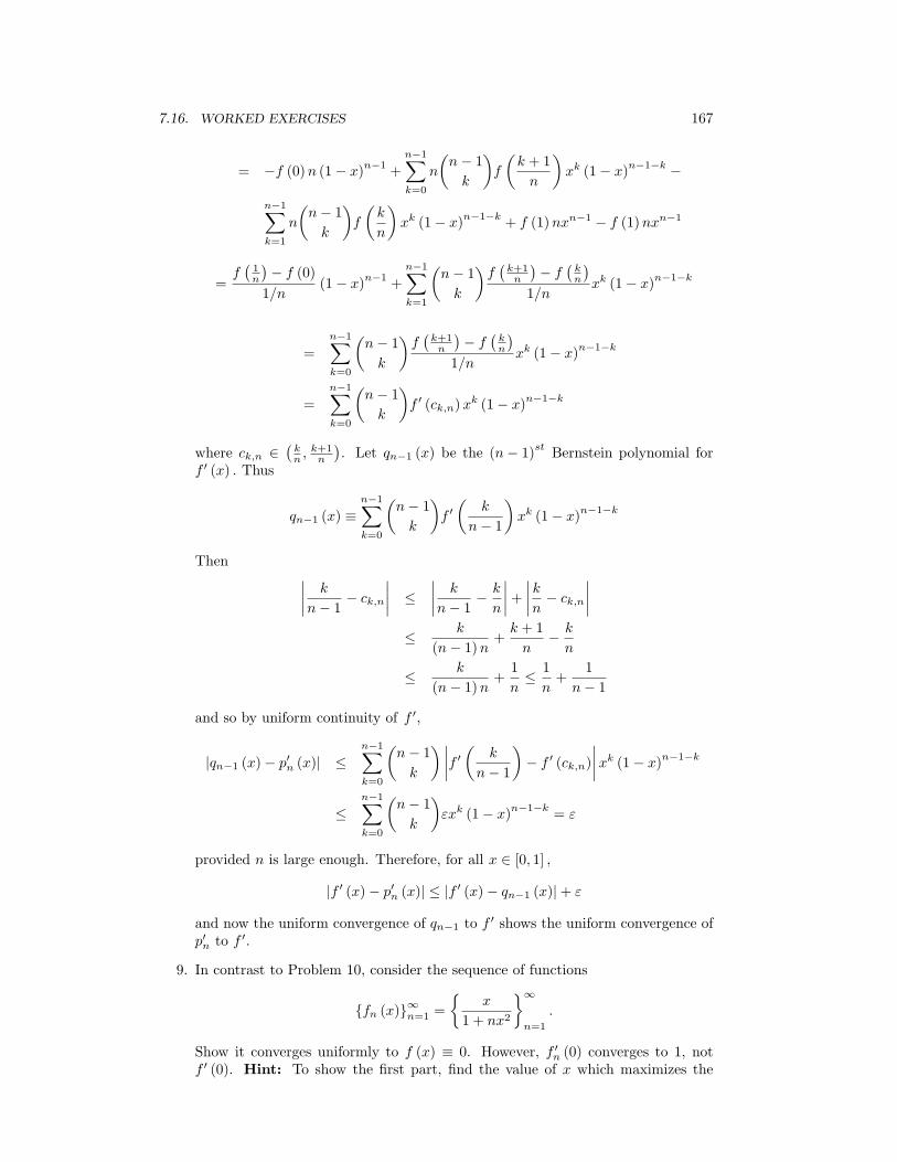
7.16. WORKED EXERCISES 167
= −f (0)n (1− x)n−1+
n−1∑k=0
n
(n− 1
k
)f
(k + 1
n
)xk (1− x)n−1−k −
n−1∑k=1
n
(n− 1
k
)f
(k
n
)xk (1− x)n−1−k
+ f (1)nxn−1 − f (1)nxn−1
=f(1n
)− f (0)
1/n(1− x)n−1
+n−1∑k=1
(n− 1
k
)f(k+1n
)− f
(kn
)1/n
xk (1− x)n−1−k
=n−1∑k=0
(n− 1
k
)f(k+1n
)− f
(kn
)1/n
xk (1− x)n−1−k
=n−1∑k=0
(n− 1
k
)f ′ (ck,n)x
k (1− x)n−1−k
where ck,n ∈(kn ,
k+1n
). Let qn−1 (x) be the (n− 1)
stBernstein polynomial for
f ′ (x) . Thus
qn−1 (x) ≡n−1∑k=0
(n− 1
k
)f ′(
k
n− 1
)xk (1− x)n−1−k
Then ∣∣∣∣ k
n− 1− ck,n
∣∣∣∣ ≤ ∣∣∣∣ k
n− 1− k
n
∣∣∣∣+ ∣∣∣∣kn − ck,n∣∣∣∣
≤ k
(n− 1)n+k + 1
n− k
n
≤ k
(n− 1)n+
1
n≤ 1
n+
1
n− 1
and so by uniform continuity of f ′,
|qn−1 (x)− p′n (x)| ≤n−1∑k=0
(n− 1
k
) ∣∣∣∣f ′( k
n− 1
)− f ′ (ck,n)
∣∣∣∣xk (1− x)n−1−k
≤n−1∑k=0
(n− 1
k
)εxk (1− x)n−1−k
= ε
provided n is large enough. Therefore, for all x ∈ [0, 1] ,
|f ′ (x)− p′n (x)| ≤ |f ′ (x)− qn−1 (x)|+ ε
and now the uniform convergence of qn−1 to f ′ shows the uniform convergence ofp′n to f ′.
9. In contrast to Problem 10, consider the sequence of functions
{fn (x)}∞n=1 =
{x
1 + nx2
}∞
n=1
.
Show it converges uniformly to f (x) ≡ 0. However, f ′n (0) converges to 1, notf ′ (0). Hint: To show the first part, find the value of x which maximizes the
168 THE DERIVATIVE
function∣∣∣ x1+nx2
∣∣∣ . You know how to do this. Then plug it in and you will have an
estimate sufficient to verify uniform convergence.
To find the value x which maximizes this is easy. You set the derivative equal to0 and find this occurs at x = 1/
√n. Then plugging this in to the formula,
|fn (x)| ≤1
2√n
and so the sequence of functions converges to 0 uniformly on R. However, thesequence of derivatives is given by
−nx2 + 1
(1 + nx2)2
and so f ′n (0) = 1 which does not converge to 0, the derivative of the targetfunction.

Power Series
8.1 Functions Defined In Terms Of Series
It is time to consider functions other than polynomials. In particular it is time to give amathematically acceptable definition of functions like ex, sin (x) and cos (x) . It has beenassumed these functions are known from beginning calculus but this is a pretence. Moststudents who take calculus come through it without a complete understanding of thecircular functions. This is because of the reliance on plane geometry in defining them.Fortunately, these functions can be completely understood in terms of power seriesrather than wretched plane geometry. The exponential function can also be defined ina simple manner using power series.
Definition 8.1.1 Let {ak}∞k=0 be a sequence of numbers. The expression,
∞∑k=0
ak (x− a)k (8.1)
is called a Taylor series centered at a. This is also called a power series centered at a.It is understood that x and a ∈ F, that is, either C or R.
In the above definition, x is a variable. Thus you can put in various values of x andask whether the resulting series of numbers converges. Defining D to be the set of allvalues of x such that the resulting series does converge, define a new function f definedon D having values in F as
f (x) ≡∞∑k=0
ak (x− a)k .
This might be a totally new function one which has no name. Nevertheless, much canbe said about such functions. The following lemma is fundamental in considering theform of D which always turns out to be of the form B (a, r) along with possibly somepoints, z such that |z − a| = r. First here is a simple lemma which will be useful.
Lemma 8.1.2 limn→∞ n1/n = 1.
Proof: It is clear n1/n ≥ 1. Let n1/n = 1 + en where 0 ≤ en. Then raising bothsides to the nth power for n > 1 and using the binomial theorem,
n = (1 + en)n=
n∑k=0
(n
k
)ekn ≥ 1 + nen + (n (n− 1) /2) e2n
≥ (n (n− 1) /2) e2n
169

170 POWER SERIES
Thus
0 ≤ e2n ≤n
n (n− 1)=
1
n− 1
From this the desired result follows because∣∣∣n1/n − 1∣∣∣ = en ≤
1√n− 1
.
Theorem 8.1.3 Let∑∞
k=0 ak (x− a)k
be a Taylor series. Then there existsr ≤ ∞ such that the Taylor series converges absolutely if |x− a| < r. Furthermore,if |x− a| > r, the Taylor series diverges.
Proof: Note
lim supk→∞
∣∣∣ak (x− a)k∣∣∣1/k = lim supk→∞
|ak|1/k |x− a| .
Then by the root test, the series converges absolutely if
|x− a| lim supk→∞
|ak|1/k < 1
and diverges if
|x− a| lim supk→∞
|ak|1/k > 1.
Thus define
r ≡
1/ lim supk→∞ |ak|
1/kif ∞ > lim supk→∞ |ak|
1/k> 0
∞ if lim supk→∞ |ak|1/k
= 0
0 if lim supk→∞ |ak|1/k
=∞
This proves the theorem.Note that the radius of convergence, r is given by
lim supk→∞
|ak|1/k r = 1
Definition 8.1.4 The number in the above theorem is called the radius of con-vergence and the set on which convergence takes place is called the disc of convergence.
Now the theorem was proved using the root test but often you use the ratio test toactually find the interval of convergence. This kind of thing is typical in math so getused to it. The proof of a theorem does not always yield a way to find the thing thetheorem speaks about. The above is an existence theorem. There exists an interval ofconvergence from the above theorem. You find it in specific cases any way that is mostconvenient.
Example 8.1.5 Find the disc of convergence of the Taylor series∑∞
n=1xn
n .
Use Corollary 5.4.10.
limn→∞
(|x|n
n
)1/n
= limn→∞
|x|n√n= |x|
because limn→∞n√n = 1 and so if |x| < 1 the series converges. The points satisfying
|z| = 1 require special attention. When x = 1 the series diverges because it reduces

8.2. OPERATIONS ON POWER SERIES 171
to∑∞
n=11n . At x = −1 the series converges because it reduces to
∑∞n=1
(−1)n
n and thealternating series test applies and gives convergence. What of the other numbers zsatisfying |z| = 1? It turns out this series will converge at all these numbers by theDirichlet test. However, this will require something like De Moivre’s theorem and thishas not yet been presented carefully.
Example 8.1.6 Find the radius of convergence of∑∞
n=1nn
n! xn.
Apply the ratio test. Taking the ratio of the absolute values of the (n+ 1)th
andthe nth terms
(n+1)(n+1)
(n+1)n! |x|n+1
nn
n! |x|n = (n+ 1)
n |x|n−n = |x|(1 +
1
n
)n
→ |x| e
Therefore the series converges absolutely if |x| e < 1 and diverges if |x| e > 1. Conse-quently, r = 1/e.
8.2 Operations On Power Series
It is desirable to be able to differentiate and multiply power series. The followingtheorem says you can differentiate power series in the most natural way on the intervalof convergence, just as you would differentiate a polynomial. This theorem may seemobvious, but it is a serious mistake to think this. You usually cannot differentiate aninfinite series whose terms are functions even if the functions are themselves polynomials.The following is special and pertains to power series. It is another example of theinterchange of two limits, in this case, the limit involved in taking the derivative andthe limit of the sequence of finite sums.
When you formally differentiate a series term by term, the result is called the derivedseries.
Theorem 8.2.1 Let∑∞
n=0 an (x− a)nbe a Taylor series having radius of con-
vergence R > 0 and let
f (x) ≡∞∑
n=0
an (x− a)n (8.2)
for |x− a| < R. Then
f ′ (x) =∞∑
n=0
ann (x− a)n−1=
∞∑n=1
ann (x− a)n−1(8.3)
and this new differentiated power series, the derived series, has radius of convergenceequal to R.
Proof: Consider g (z) =∑∞
k=2 akk (z − a)k−1
on B (a,R) where R is the radius ofconvergence defined above. Let r1 < r < R. Then letting |z − a| < r1 and h < r − r1,∣∣∣∣f (z + h)− f (z)
h− g (z)
∣∣∣∣≤
∞∑k=2
|ak|
∣∣∣∣∣ (z + h− a)k − (z − a)k
h− k (z − a)k−1
∣∣∣∣∣≤
∞∑k=2
|ak|
∣∣∣∣∣ 1h(
k∑i=0
(k
i
)(z − a)k−i
hi − (z − a)k)− k (z − a)k−1
∣∣∣∣∣=
∞∑k=2
|ak|
∣∣∣∣∣ 1h(
k∑i=1
(k
i
)(z − a)k−i
hi
)− k (z − a)k−1
∣∣∣∣∣
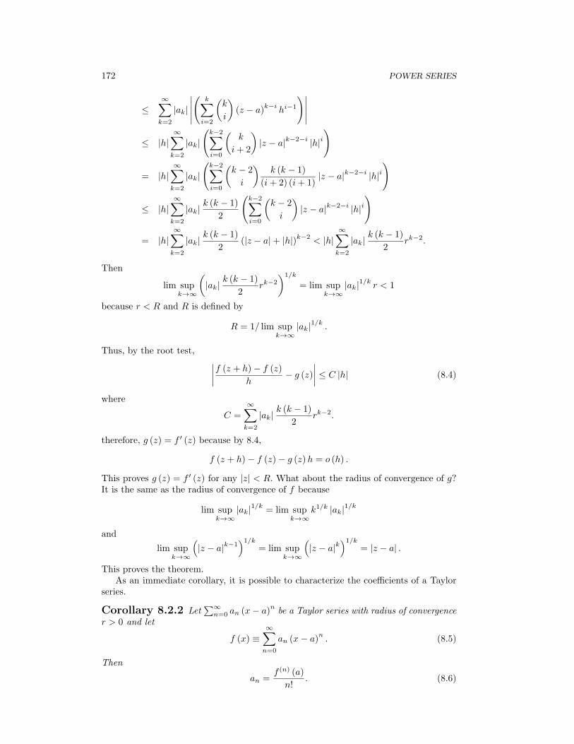
172 POWER SERIES
≤∞∑k=2
|ak|
∣∣∣∣∣(
k∑i=2
(k
i
)(z − a)k−i
hi−1
)∣∣∣∣∣≤ |h|
∞∑k=2
|ak|
(k−2∑i=0
(k
i+ 2
)|z − a|k−2−i |h|i
)
= |h|∞∑k=2
|ak|
(k−2∑i=0
(k − 2
i
)k (k − 1)
(i+ 2) (i+ 1)|z − a|k−2−i |h|i
)
≤ |h|∞∑k=2
|ak|k (k − 1)
2
(k−2∑i=0
(k − 2
i
)|z − a|k−2−i |h|i
)
= |h|∞∑k=2
|ak|k (k − 1)
2(|z − a|+ |h|)k−2
< |h|∞∑k=2
|ak|k (k − 1)
2rk−2.
Then
lim supk→∞
(|ak|
k (k − 1)
2rk−2
)1/k
= lim supk→∞
|ak|1/k r < 1
because r < R and R is defined by
R = 1/ lim supk→∞
|ak|1/k .
Thus, by the root test, ∣∣∣∣f (z + h)− f (z)h
− g (z)∣∣∣∣ ≤ C |h| (8.4)
where
C =∞∑k=2
|ak|k (k − 1)
2rk−2.
therefore, g (z) = f ′ (z) because by 8.4,
f (z + h)− f (z)− g (z)h = o (h) .
This proves g (z) = f ′ (z) for any |z| < R. What about the radius of convergence of g?It is the same as the radius of convergence of f because
lim supk→∞
|ak|1/k = lim supk→∞
k1/k |ak|1/k
and
lim supk→∞
(|z − a|k−1
)1/k= lim sup
k→∞
(|z − a|k
)1/k= |z − a| .
This proves the theorem.As an immediate corollary, it is possible to characterize the coefficients of a Taylor
series.
Corollary 8.2.2 Let∑∞
n=0 an (x− a)nbe a Taylor series with radius of convergence
r > 0 and let
f (x) ≡∞∑
n=0
an (x− a)n . (8.5)
Then
an =f (n) (a)
n!. (8.6)

8.3. THE SPECIAL FUNCTIONS OF ELEMENTARY CALCULUS 173
Proof: From 8.5, f (a) = a0 ≡ f (0) (a) /0!. From Theorem 8.2.1,
f ′ (x) =
∞∑n=1
ann (x− a)n−1= a1 +
∞∑n=2
ann (x− a)n−1.
Now let x = a and obtain that f ′ (a) = a1 = f ′ (a) /1!. Next use Theorem 8.2.1 againto take the second derivative and obtain
f ′′ (x) = 2a2 +
∞∑n=3
ann (n− 1) (x− a)n−2
let x = a in this equation and obtain a2 = f ′′ (a) /2 = f ′′ (a) /2!. Continuing this wayproves the corollary.
This also shows the coefficients of a Taylor series are unique. That is, if
∞∑k=0
ak (x− a)k =∞∑k=0
bk (x− a)k
for all x in some open set containing a, then ak = bk for all k.
Example 8.2.3 Find the sum∑∞
k=1 k2−k.
It may not be obvious what this sum equals but with the above theorem it is easyto find. From the formula for the sum of a geometric series, 1
1−t =∑∞
k=0 tk if |t| < 1.
Differentiate both sides to obtain
(1− t)−2=
∞∑k=1
ktk−1
whenever |t| < 1. Let t = 1/2. Then
4 =1
(1− (1/2))2 =
∞∑k=1
k2−(k−1)
and so if you multiply both sides by 2−1,
2 =
∞∑k=1
k2−k.
8.3 The Special Functions Of Elementary Calculus
8.3.1 The Functions, sin, cos, exp
With this material on power series, it becomes possible to give an understandable treat-ment of the exponential function exp and the circular functions, sin and cos .
Definition 8.3.1 Define for all x ∈ R
sin (x) ≡∞∑k=0
(−1)k x2k+1
(2k + 1)!, cos (x) ≡
∞∑k=0
(−1)k x2k
(2k)!
exp (x) ≡∞∑k=0
xk
k!.
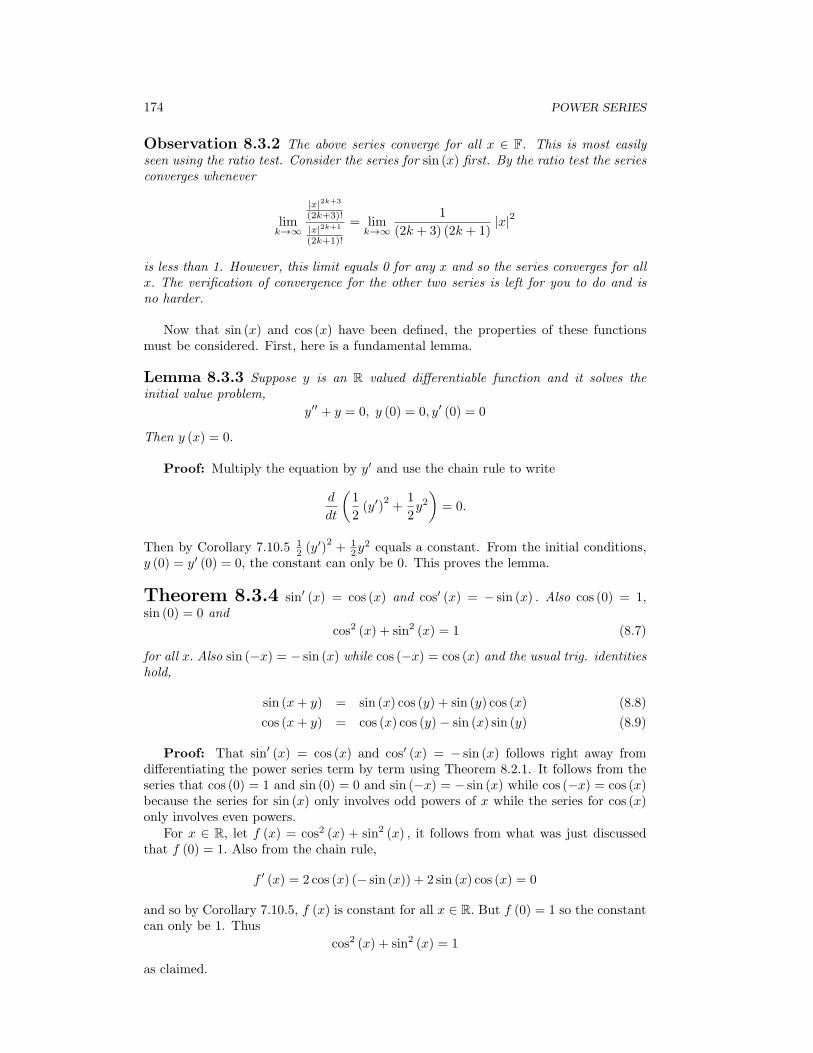
174 POWER SERIES
Observation 8.3.2 The above series converge for all x ∈ F. This is most easilyseen using the ratio test. Consider the series for sin (x) first. By the ratio test the seriesconverges whenever
limk→∞
|x|2k+3
(2k+3)!
|x|2k+1
(2k+1)!
= limk→∞
1
(2k + 3) (2k + 1)|x|2
is less than 1. However, this limit equals 0 for any x and so the series converges for allx. The verification of convergence for the other two series is left for you to do and isno harder.
Now that sin (x) and cos (x) have been defined, the properties of these functionsmust be considered. First, here is a fundamental lemma.
Lemma 8.3.3 Suppose y is an R valued differentiable function and it solves theinitial value problem,
y′′ + y = 0, y (0) = 0, y′ (0) = 0
Then y (x) = 0.
Proof: Multiply the equation by y′ and use the chain rule to write
d
dt
(1
2(y′)
2+
1
2y2)
= 0.
Then by Corollary 7.10.5 12 (y
′)2+ 1
2y2 equals a constant. From the initial conditions,
y (0) = y′ (0) = 0, the constant can only be 0. This proves the lemma.
Theorem 8.3.4 sin′ (x) = cos (x) and cos′ (x) = − sin (x) . Also cos (0) = 1,sin (0) = 0 and
cos2 (x) + sin2 (x) = 1 (8.7)
for all x. Also sin (−x) = − sin (x) while cos (−x) = cos (x) and the usual trig. identitieshold,
sin (x+ y) = sin (x) cos (y) + sin (y) cos (x) (8.8)
cos (x+ y) = cos (x) cos (y)− sin (x) sin (y) (8.9)
Proof: That sin′ (x) = cos (x) and cos′ (x) = − sin (x) follows right away fromdifferentiating the power series term by term using Theorem 8.2.1. It follows from theseries that cos (0) = 1 and sin (0) = 0 and sin (−x) = − sin (x) while cos (−x) = cos (x)because the series for sin (x) only involves odd powers of x while the series for cos (x)only involves even powers.
For x ∈ R, let f (x) = cos2 (x) + sin2 (x) , it follows from what was just discussedthat f (0) = 1. Also from the chain rule,
f ′ (x) = 2 cos (x) (− sin (x)) + 2 sin (x) cos (x) = 0
and so by Corollary 7.10.5, f (x) is constant for all x ∈ R. But f (0) = 1 so the constantcan only be 1. Thus
cos2 (x) + sin2 (x) = 1
as claimed.
8.3. THE SPECIAL FUNCTIONS OF ELEMENTARY CALCULUS 175
It only remains to verify the identities. Consider 8.8 first. Fixing y and consideringboth sides as a function of x, it follows from the above that both sides of the identitysatisfy the initial value problem
y′′ + y = 0, y (0) = sin (y) , y′ (0) = cos (y)
Therefore, the difference satisfies the initial value problem of Lemma 8.3.3. Therefore,by this lemma, the difference equals 0. The next identity is handled similarly. Thisproves the theorem.
Proposition 8.3.5 The following important limits hold for a, b = 0.
limx→0
sin (ax)
bx=a
b, lim
x→0
1− cos (x)
x= 0.
Proof: From the definition of sin (x) given above,
sin (ax)
bx=
∑∞k=0 (−1)
k (ax)2k+1
(2k+1)!
bx=ax+
∑∞k=1 (−1)
k (ax)2k+1
(2k+1)!
bx
=a+
∑∞k=1 (−1)
k (ax)2k
(2k+1)!
b
Now ∣∣∣∣∣∞∑k=1
(−1)k (ax)2k
(2k + 1)!
∣∣∣∣∣ ≤∞∑k=1
|ax|2k =∞∑k=1
(|ax|2
)k=
(|ax|2
1− |ax|
)
whenever |ax| < 1. Thus
limx→0
∞∑k=1
(−1)k (ax)2k
(2k + 1)!= 0
and so
limx→0
sin (ax)
bx=a
b.
The other limit can be handled similarly.It is possible to verify the functions are periodic.
Lemma 8.3.6 There exists a positive number, a, such that cos (a) = 0.
Proof:To prove this, note that cos (0) = 1 and so if it is false, it must be the casethat cos (x) > 0 for all positive x since otherwise, it would follow from the intermediatevalue theorem there would exist a point, x where cosx = 0. Assume cos (x) > 0 forall x. Then by Corollary 7.10.6 it would follow that t → sin t is a strictly increasingfunction on (0,∞) . Also note that sin (0) = 0 and so sin (x) > 0 for all x > 0. This isbecause, by the mean value theorem there exists t ∈ (0, x) such that
sin (x) = sin (x)− sin (0) = (cos (t)) (x− 0) > 0.
By 8.7, |f (x)| ≤ 1 for f = cos and sin . Let 0 < x < y. Then from the mean valuetheorem,
− cos (y)− (− cos (x)) = sin (t) (y − x)
176 POWER SERIES
for some t ∈ (x, y) . Since t→ sin (t) is increasing, it follows
− cos (y)− (− cos (x)) = sin (t) (y − x) ≥ sin (x) (y − x) .
This contradicts the inequality |cos (y)| ≤ 1 for all y because the right side is unboundedas y →∞. This proves the lemma.
Theorem 8.3.7 Both cos and sin are periodic.
Proof: Define a number, π such that
π
2≡ inf {x : x > 0 and cos (x) = 0}
Then π2 > 0 because cos (0) = 1 and cos is continuous. On
[0, π2
]cos is positive and so
it follows sin is increasing on this interval. Therefore, from 8.7, sin(π2
)= 1. Now from
Theorem 8.3.4,
cos (π) = cos(π2+π
2
)= − sin2
(π2
)= −1, sin (π) = 0
Using Theorem 8.3.4 again,
cos (2π) = cos2 (π) = 1 = cos (0) ,
and so sin (2π) = 0. From Theorem 8.3.4,
cos (x+ 2π) = cos (x) cos (2π)− sin (x) sin (2π) = cos (x)
Thus cos is periodic of period 2π. By Theorem 8.3.4,
sin (x+ 2π) = sin (x) cos (2π) + cos (x) sin (2π) = sin (x)
Using 8.7, it follows sin is also periodic of period 2π. This proves the theorem.Note that 2π is the smallest period for these functions. This can be seen by observing
that the above theorem and proof imply that cos is positive on(0,π
2
),
(3π
2, 2π
)and negative on
(π2 ,
3π2
)and that similar observations on sin are valid. Also, by consid-
ering where these functions are equal to 0, 1, and -1 along with where they are positiveand negative, it follows that whenever a2+ b2 = 1, there exists a unique t ∈ [0, 2π) suchthat cos (t) = a and sin (t) = b. For example, if a and b are both positive, then sincecos is continuous and strictly decreases from 1 to 0 on
[0, π2
], it follows there exists a
unique t ∈ (0, π/2) such that cos (t) = a. Since b > 0 and sin is positive on (0, π/2) ,it follows sin (t) = b. No other value of t in [0,2π) will work since only on (0, π/2) areboth cos and sin positive. If a > 0 and b < 0 similar reasoning will show there exists aunique t ∈ [0, 2π) with cos (t) = a and sin (t) = b and in this case, t ∈ (3π/2, 2π) . Othercases are similar and are left to the reader. Thus, every point on the unit circle is ofthe form (cos t, sin t) for a unique t ∈ [0, 2π).
This shows the unit circle is a smooth curve, however this notion will not be consid-ered here.
Corollary 8.3.8 For all x ∈ F
sin (x+ 2π) = sin (x) , cos (x+ 2π) = cos (x)

8.3. THE SPECIAL FUNCTIONS OF ELEMENTARY CALCULUS 177
Proof: Let y (x) ≡ sin (x+ 2π) − sin (x) . Then from what has been shown above,y′ (0) = y (0) = 0. It is also clear from the above that y′′ + y = 0. Therefore, fromLemma 8.3.3 y = 0. Differentiating the identity just obtained yields the second identity.This proves the corollary.
Are these the same as the circular functions you studied very sloppily in calculusand trigonometry? They are.
If sin (x) defined above and sin (x) studied in a beginning calculus class both satisfythe initial value problem
y′′ + y = 0, y (0) = 0, y′ (0) = 1
then they must be the same. However, if you remember anything from calculus youwill realize sin (x) used there does satisfy the above initial value problem. If you don’tremember anything from calculus, then it does not matter about harmonizing the func-tions. Just use the definition given above in terms of a power series. Similar considera-tions apply to cos .
Of course all the other trig. functions are defined as earlier. Thus
tanx =sinx
cosx, cotx ≡ cosx
sinx, secx ≡ 1
cosx, cscx ≡ 1
sinx.
Using the techniques of differentiation, you can find the derivatives of all these.Now it is time to consider the exponential function exp (x) defined above. To do
this, it is convenient to have the following uniqueness theorem.
Lemma 8.3.9 Supposey′ − y = 0, y (0) = 0
Then y = 0. Also for all x ∈ R, exp(−x)(exp(x)) = 1
Proof: The function exp has been defined above in terms of a power series. Fromthis power series and Theorem 8.2.1 it follows that exp solves the above initial valueproblem. Multiply both sides of the differential equation by exp (−x) . Then using thechain rule and product rule,
d
dx(exp (−x) y (x)) = 0
and so exp (−x) y (x) = C, a constant. The constant can only be 0 because of the initialcondition. Therefore,
exp (−x) y (x) = 0
for all x.Now I claim exp (−x) and exp (x) are never equal to 0. This is because by the chain
rule, abusing notation slightly,
(exp (−x) exp (x))′ = − exp (−x) exp (x) + exp (−x) exp (x) = 0
and soexp (−x) exp (x) = C
a constant. However, this constant can only be 1 because this is what it is when x = 0,a fact which follows right away from the definition in terms of power series. This provesthe lemma.
Theorem 8.3.10 The function exp satisfies the following properties.
1. exp (x) > 0 for all x ∈ R, limx→∞ exp (x) =∞, limx→−∞ exp (x) = 0.

178 POWER SERIES
2. exp is the unique solution to the initial value problem
y′ − y = 0, y (0) = 1 (8.10)
3. For all x, y ∈ Fexp (x+ y) = exp (x) exp (y) (8.11)
4. exp is one to one mapping R onto (0,∞) .
Proof: To begin with consider 8.11. Fixing y it follows from the chain rule and thedefinition using power series that
x→ exp (x+ y)− exp (x) exp (y)
satisfies the initial value problem of Lemma 8.3.9 and so it is 0. This shows 8.11.
8.10 has already been noted. It comes directly from the definition and was provedin Lemma 8.3.9. The claim that exp (x) > 0 was also established in the proof of thislemma.
Now from the power series, it is obvious that exp (x) > 0 if x > 0 and by Lemma
8.3.9, exp (x)−1
= exp (−x) , so it follows exp (−x) is also positive. Since exp (x) >∑2k=0
xk
k! , it is clear limx→∞ exp (x) =∞ and it follows from this that limx→−∞ exp (x) =0.
It only remains to verify 4. Let y ∈ (0,∞) . From the earlier properties, there existx1 such that exp (x1) < y and x2 such that exp (x2) > y. Then by the intermediatevalue theorem, there exists x ∈ (x1, x2) such that exp (x) = y. Thus exp maps onto(0,∞). It only remains to verify exp is one to one. Suppose then that x1 < x2. By themean value theorem, there exists x ∈ (x1, x2) such that
exp (x) (x2 − x1) = exp′ (x) (x2 − x1) = exp (x2)− exp (x1) .
Since exp (x) > 0, it follows exp (x2) = exp (x1). This proves the theorem.
8.3.2 ln And logb
In this section, the inverse function of x→ exp (x) is considered.
Definition 8.3.11 ln is the inverse function of exp . Thus ln : (0,∞) → R ,ln (exp (x)) = x, and exp (ln (x)) = x. The number e is that number such that ln (e) = 1.
By Corollary 7.13.2, it follows ln is differentiable. This makes possible the followingsimple theorem.
Theorem 8.3.12 The following basic properties are available for ln .
ln′ (x) =1
x. (8.12)
Also for all x, y > 0,
ln (xy) = ln (x) + ln (y) , (8.13)
ln (1) = 0, ln (xm) = m ln (x) (8.14)
for all m an integer.
8.3. THE SPECIAL FUNCTIONS OF ELEMENTARY CALCULUS 179
Proof: Since exp (ln (x)) = x and ln′ exists, it follows
x ln′ (x) = exp (ln (x)) ln′ (x) = exp′ (ln (x)) ln′ (x) = 1
and this proves 8.12. Next consider 8.13.
xy = exp (ln (xy)) , exp (ln (x) + ln (y)) = exp (ln (x)) exp (ln (y)) = xy.
Since exp was shown to be 1-1, it follows ln (xy) = ln (x) + ln (y) . Next exp (0) = 1 andexp (ln (1)) = 1 so ln (1) = 0 again because exp is 1-1. Let
f (x) = ln (xm)−m ln (x) .
f (1) = ln (1)−m ln (1) = 0. Also, by the chain rule,
f ′ (x) =1
xmmxm−1 −m 1
x= 0
and so f (x) equals a constant. The constant can only be 0 because f (1) = 0. Thisproves the last formula of 8.14 and completes the proof of the theorem.
The last formula tells how to define xα for any x > 0 and α ∈ R. I want to stress thisis something new. Students are often deceived into thinking they know what xα meansfor α a real number. There is no place for such deception in mathematics, however.
Definition 8.3.13 Define xα for x > 0 and α ∈ R by the following formula.
ln (xα) = α ln (x) .
In other words,xα ≡ exp (α ln (x)) .
From Theorem 8.3.12 this new definition does not contradict the usual definition inthe case where α is an integer.
From this definition, the following properties are obtained.
Proposition 8.3.14 For x > 0 let f (x) = xα where α ∈ R. Then f ′ (x) = αxα−1.
Also xα+β = xαxβ and (xα)β= xαβ.
Proof: First consider the claim about the sum of the exponents.
xα+β ≡ exp ((α+ β) ln (x)) = exp (α ln (x) + β ln (x))
= exp (α ln (x)) exp (β ln (x)) ≡ xαxβ .
ln((xα)
β)= β ln (xα) = αβ ln (x) , ln
(xαβ
)= αβ ln (x) .
The claim about the derivative follows from the chain rule. f (x) = exp (α ln (x)) andso
f ′ (x) = exp (α ln (x))α
x≡ α
xxα = α
(x−1
)xα = αxα−1.
This proves the proposition.
Definition 8.3.15 Define logb for any b > 0, b = 1 by
logb (x) ≡ln (x)
ln (b).
Proposition 8.3.16 The following hold for logb (x) .
180 POWER SERIES
1. blogb(x) = x, logb (bx) = x.
2. logb (xy) = logb (x) + logb (y)
3. logb (xα) = α logb (x)
Proof:
blogb(x) ≡ exp (ln (b) logb (x)) = exp
(ln (b)
ln (x)
ln (b)
)= exp (ln (x)) = x
logb (bx) =
ln (bx)
ln (b)=x ln (b)
ln (b)= x
This proves 1.Now consider 2.
logb (xy) =ln (xy)
ln (b)=
ln (x)
ln (b)+
ln (y)
ln (b)= logb (x) + logb (y) .
Finally,
logb (xα) =
ln (xα)
ln (b)= α
ln (x)
ln (b)= α logb (x) .
8.4 The Binomial Theorem
The following is a very important example known as the binomial series.
Example 8.4.1 Find a Taylor series for the function (1 + x)αcentered at 0 valid for
|x| < 1.
Use Theorem 8.2.1 to do this. First note that if y (x) ≡ (1 + x)α, then y is a solution
of the following initial value problem.
y′ − α
(1 + x)y = 0, y (0) = 1. (8.15)
Next it is necessary to observe there is only one solution to this initial value problem.To see this, multiply both sides of the differential equation in 8.15 by (1 + x)
−α. When
this is done one obtains
d
dx
((1 + x)
−αy)= (1 + x)
−α
(y′ − α
(1 + x)y
)= 0. (8.16)
Therefore, from 8.16, there must exist a constant, C, such that
(1 + x)−α
y = C.
However, y (0) = 1 and so it must be that C = 1. Therefore, there is exactly one solutionto the initial value problem in 8.15 and it is y (x) = (1 + x)
α.
The strategy for finding the Taylor series of this function consists of finding a serieswhich solves the initial value problem above. Let
y (x) ≡∞∑
n=0
anxn (8.17)

8.4. THE BINOMIAL THEOREM 181
be a solution to 8.15. Of course it is not known at this time whether such a series exists.However, the process of finding it will demonstrate its existence. From Theorem 8.2.1and the initial value problem,
(1 + x)
∞∑n=0
annxn−1 −
∞∑n=0
αanxn = 0
and so∞∑
n=1
annxn−1 +
∞∑n=0
an (n− α)xn = 0
Changing the variable of summation in the first sum,
∞∑n=0
an+1 (n+ 1)xn +∞∑
n=0
an (n− α)xn = 0
and from Corollary 8.2.2 and the initial condition for 8.15 this requires
an+1 =an (α− n)n+ 1
, a0 = 1. (8.18)
Therefore, from 8.18 and letting n = 0, a1 = α, then using 8.18 again along with thisinformation,
a2 =α (α− 1)
2.
Using the same process,
a3 =
(α(α−1)
2
)(α− 2)
3=α (α− 1) (α− 2)
3!.
By now you can spot the pattern. In general,
an =
n of these factors︷ ︸︸ ︷α (α− 1) · · · (α− n+ 1)
n!.
Therefore, the candidate for the Taylor series is
y (x) =∞∑
n=0
α (α− 1) · · · (α− n+ 1)
n!xn.
Furthermore, the above discussion shows this series solves the initial value problem onits interval of convergence. It only remains to show the radius of convergence of thisseries equals 1. It will then follow that this series equals (1 + x)
αbecause of uniqueness
of the initial value problem. To find the radius of convergence, use the ratio test. Thusthe ratio of the absolute values of (n+ 1)
stterm to the absolute value of the nth term
is ∣∣∣α(α−1)···(α−n+1)(α−n)(n+1)n!
∣∣∣ |x|n+1∣∣∣α(α−1)···(α−n+1)n!
∣∣∣ |x|n = |x| |α− n|n+ 1
→ |x|
showing that the radius of convergence is 1 since the series converges if |x| < 1 anddiverges if |x| > 1.
The expression, α(α−1)···(α−n+1)n! is often denoted as
(αn
). With this notation, the
following theorem has been established.
182 POWER SERIES
Theorem 8.4.2 Let α be a real number and let |x| < 1. Then
(1 + x)α=
∞∑n=0
(α
n
)xn.
There is a very interesting issue related to the above theorem which illustrates thelimitation of power series. The function f (x) = (1 + x)
αmakes sense for all x > −1
but one is only able to describe it with a power series on the interval (−1, 1) . Thinkabout this. The above technique is a standard one for obtaining solutions of differentialequations and this example illustrates a deficiency in the method.
To completely understand power series, it is necessary to take a course in complexanalysis. It turns out that the right way to consider Taylor series is through the use ofgeometric series and something called the Cauchy integral formula of complex analysis.However, these are topics for another course.
8.5 Exercises
1. In each of the following, assume the relation defines y as a function of x for valuesof x and y of interest and find y′ (x) .
(a) xy2 + sin (y) = x3 + 1
(b) y3 + x cos(y2)= x4
(c) y cos (x) = tan (y) cos(x2)+ 2
(d)(x2 + y2
)6= x3y + 3
(e) xy2+yy5+x + cos (y) = 7
(f)√x2 + y4 sin (y) = 3x
(g) y3 sin (x) + y2x2 = 2x2
y + ln |y|(h) y2 sin (y)x+ log3 (xy) = y2 + 11
(i) sin(x2 + y2
)+ sec (xy) = ex+y + y2y + 2
(j) sin(tan
(xy2))
+ y3 = 16
(k) cos (sec (tan (y))) + ln (5 + sin (xy)) = x2y + 3
2. In each of the following, assume the relation defines y as a function of x for valuesof x and y of interest. Use the chain rule to show y satisfies the given differentialequation.
(a) x2y + sin y = 7,(x2 + cos y
)y′ + 2xy = 0.
(b) x2y3 + sin(y2)= 5, 2xy3 +
(3x2y2 + 2
(cos(y2))y)y′ = 0.
(c) y2 sin (y) + xy = 6,(2y (sin (y)) + y2 (cos (y)) + x
)y′ + y = 0.
3. Show that if D (g) ⊆ U ⊆ D (f) , and if f and g are both one to one, then f ◦ g isalso one to one.
4. The number e is that number such that ln e = 1. Prove ex = exp (x) .
5. Find a formula for dydx for y = bx. Prove your formula.
8.5. EXERCISES 183
6. Let y = xx for x ∈ R. Find y′ (x) .
7. The logarithm test states the following. Suppose ak = 0 for large k and that
p = limk→∞ln
(1
|ak|
)ln k exists. If p > 1, then
∑∞k=1 ak converges absolutely. If
p < 1, then the series,∑∞
k=1 ak does not converge absolutely. Prove this theorem.
8. Suppose f (x+ y) = f (x) + f (y) and f is continuous at 0. Find all solutions tothis functional equation which are continuous at x = 0. Now find all solutionswhich are bounded near 0. Next if you want an even more interesting version ofthis, find all solutions whose graphs are not dense in the plane. (A set S is densein the plane if for every (a, b) ∈ R×R and r > 0, there exists (x, y) ∈ S such that√
(x− a)2 + (y − b)2 < r.)
This is called the Cauchy equation.
9. Suppose f (x+ y) = f (x) f (y) and f is continuous and not identically zero. Findall solutions to this functional equation. Hint: First show the functional equationrequires f > 0.
10. Suppose f (xy) = f (x)+ f (y) for x, y > 0. Suppose also f is continuous. Find allsolutions to this functional equation.
11. Using the Cauchy condensation test, determine the convergence of∑∞
k=21
k ln k .Now determine the convergence of
∑∞k=2
1k(ln k)1.001
.
12. Find the values of p for which the following series converges and the values of pfor which it diverges.
∞∑k=4
1
lnp (ln (k)) ln (k) k
13. For p a positive number, determine the convergence of
∞∑n=2
lnn
np
for various values of p.
14. Determine whether the following series converge absolutely, conditionally, or notat all and give reasons for your answers.
(a)∑∞
n=1 (−1)n ln(k5)
k
(b)∑∞
n=1 (−1)n ln(k5)
k1.01
(c)∑∞
n=1 (−1)n 10n
(1.01)n
(d)∑∞
n=1 (−1)nsin(1n
)(e)
∑∞n=1 (−1)
ntan
(1n2
)(f)
∑∞n=1 (−1)
ncos(
1n2
)(g)
∑∞n=1 (−1)
nsin( √
nn2+1
)
184 POWER SERIES
15. De Moivre’s theorem says
[r (cos t+ i sin t)]n= rn (cosnt+ i sinnt)
for n a positive integer. Prove this formula by induction. Does this formulacontinue to hold for all integers, n, even negative integers? Explain.
16. Using De Moivre’s theorem, show that if z ∈ C then z has n distinct nth roots.Hint: Letting z = x+ iy,
z = |z|(x
|z|+ i
y
|z|
)and argue
(x|z| ,
y|z|
)is a point on the unit circle. Hence z = |z| (cos (θ) + i sin (θ)) .
Then
w = |w| (cos (α) + i sin (α))
is an nth root if and only if (|w| (cos (α) + i sin (α)))n= z. Show this happens
exactly when |w| = n√|z| and α = θ+2kπ
n for k = 0, 1, · · · , n.
17. Using De Moivre’s theorem from Problem 15, derive a formula for sin (5x) andone for cos (5x).
18. Suppose∑∞
n=0 an (x− c)nis a power series with radius of convergence r. Show
the series converge uniformly on any interval [a, b] where [a, b] ⊆ (c− r, c+ r) .
19. Find the disc of convergence of the series∑
xn
np for various values of p. Hint: UseDirichlet’s test.
20. Show
ex =∞∑k=0
xk
k!
for all x ∈ R where e is the number such that ln e = 1. Thus
e =∞∑k=0
1
k!.
Show e is irrational. Hint: If e = p/q for p, q positive integers, then argue
q!
(p
q−
q∑k=0
1
k!
)
is an integer. However, you can also show
q!
( ∞∑k=0
1
k!−
q∑k=0
1
k!
)< 1
21. Let a ≥ 1. Show that for all x > 0, you have the inequality
ax > ln (1 + xa) .
8.6. WORKED EXERCISES 185
8.6 Worked Exercises
1. The number e is that number such that ln e = 1. Prove ex = exp (x) .
ex ≡ exp (x ln (e)) ≡ exp (x)
2. Let y = xx for x ∈ R. Find y′ (x) .ln (y) = x lnx and so y′ 1y = x 1
x + ln (x) and so
y′ = xx (1 + ln (x)) .
3. The logarithm test states the following. Suppose ak = 0 for large k and that
p = limk→∞ln
(1
|ak|
)ln k exists. If p > 1, then
∑∞k=1 ak converges absolutely. If
p < 1, then the series,∑∞
k=1 ak does not converge absolutely. Prove this theorem.
If p > 1, then for all k large enough,
ln
(1
|ak|
)> r ln (k) = ln (kr)
for p > r > 1. Therefore, for all k large enough,
1
|ak|> kr so |ak| <
1
kr
Hence convergence takes place by comparison to the series∑
1kr . Next suppose
p < 1. Then similar to the above, for all k large enough,
ln
(1
|ak|
)< ln (kr) , |ak| >
1
kr
for some r < 1 and so divergence takes place by comparison to the series∑
1kr
where r < 1.
4. Suppose f (x+ y) = f (x) + f (y) and f is continuous at 0. Find all solutions tothis functional equation which are continuous at x = 0. Now find all solutionswhich are bounded near 0. Next if you want an even more interesting version ofthis, find all solutions whose graphs are not dense in the plane. (A set S is densein the plane if for every (a, b) ∈ R×R and r > 0, there exists (x, y) ∈ S such that√
(x− a)2 + (y − b)2 < r.)
This is called the Cauchy equation.
Most of this is easy. If it is continuous at 0 then you can use the functional equationto show it is continuous everywhere. Then you can show from the functionalequation that f (x) = kx where k = f (1). You do this by considering x rationalfirst and then using continuity and density of the rationals to obtain it for allx. Suppose now you only know |f (x)| < M for all |x| < r. Let xn → 0. Thenthere exists a sequence of integers Cn such that Cn → ∞ but Cnxn ∈ (−r, r).Therefore, from the functional equation
|f (xn)Cn| < M
and so f (xn) → 0 which forces f to be continuous at 0 and now the first partimplies f is continuous and is of the form f (x) = xf (1). A similar argumentshows that f has this form if it is bounded on any finite interval.
186 POWER SERIES
5. Suppose f (x+ y) = f (x) f (y) and f is continuous and not identically zero. Findall solutions to this functional equation. Hint: First show the functional equationrequires f > 0.
f (2x) = f (x)2and so f (y) ≥ 0 for all y. Could f (x) = 0? If so, then f (mx) =
f (x)m
= 0 and also it is routine to show that f(
kmx)= f (x)
k/mwhenever
k,m are integers. Hence by continuity, f (x) ≡ 0 so it can’t ever vanish. Nowif F (x) = ln (f (x)) , Then F (x+ y) = F (x) + F (y) and so from the previousproblem,
F (x) = kx, f (x) = ekx
6. For p a positive number, determine the convergence of
∞∑n=2
lnn
np
for various values of p.
You could use the Cauchy condensation test. Convergence is the same as for
∑ 2nn ln (2)
2np
Then use the root test. If p > 1 it converges. If p < 1 it diverges. If p = 1 itobviously diverges by comparison to
∑1/n.
7. Suppose∑∞
n=0 an (x− c)nis a power series with radius of convergence r. Show
the series converge uniformly on any interval [a, b] where [a, b] ⊆ (c− r, c+ r) .
Let r1 be close enough to r that c− r < c− r1 < a < b < c+ r1 < c+ r. Then forx ∈ [a, b]
|an| |x− c|n ≤ |an| rn1
Now lim sup |an|1/n r1 < lim sup |an|1/n 1lim sup|an|1/n
= 1 by definition of r and the
fact r1 < r. Thus∑
n |an| rn1 converges and so by the Weierstrass M test, theseries converges uniformly for x ∈ [a, b].
8. Find the disc of convergence of the series∑
xn
np for various values of p. Hint: UseDirichlet’s test.
The radius of convergence is 1. It only remains to verify what happens at boundarypoints. If x = 1 the series converges if p > 1 and diverges if p ≤ 1. Letting|ω| = 1, ω = 1, what about ∑ ωn
np?
It turns out this converges for all such ω. This follows from
n∑k=0
ωk =ωn+1
ω − 1− 1
ω − 1
and this is bounded. In fact, it is smaller than 2/ |ω − 1| . Therefore, the Dirichlettest applies.
8.7. L’HOPITAL’S RULE 187
8.7 L’Hopital’s Rule
There is an interesting rule which is often useful for evaluating difficult limits calledL’Hopital’s1 rule. The best versions of this rule are based on the Cauchy Mean valuetheorem, Theorem 7.10.2 on Page 153.
Theorem 8.7.1 Let [a, b] ⊆ [−∞,∞] and suppose f, g are functions which sat-isfy,
limx→b−
f (x) = limx→b−
g (x) = 0, (8.19)
and f ′ and g′ exist on (a, b) with g′ (x) = 0 on (a, b). Suppose also that
limx→b−
f ′ (x)
g′ (x)= L. (8.20)
Then
limx→b−
f (x)
g (x)= L. (8.21)
Proof: By the definition of limit and 8.20 there exists c < b such that if t > c, then∣∣∣∣f ′ (t)g′ (t)− L
∣∣∣∣ < ε
2.
Now pick x, y such that c < x < y < b. By the Cauchy mean value theorem, thereexists t ∈ (x, y) such that
g′ (t) (f (x)− f (y)) = f ′ (t) (g (x)− g (y)) .
Since g′ (s) = 0 for all s ∈ (a, b) it follows from the mean value theorem g (x)−g (y) = 0.Therefore,
f ′ (t)
g′ (t)=f (x)− f (y)g (x)− g (y)
and so, since t > c, ∣∣∣∣f (x)− f (y)g (x)− g (y)− L
∣∣∣∣ < ε
2.
Now letting y → b−, ∣∣∣∣f (x)g (x)− L
∣∣∣∣ ≤ ε
2< ε.
Since ε > 0 is arbitrary, this shows 8.21.The following corollary is proved in the same way.
Corollary 8.7.2 Let [a, b] ⊆ [−∞,∞] and suppose f, g are functions which satisfy,
limx→a+
f (x) = limx→a+
g (x) = 0, (8.22)
and f ′ and g′ exist on (a, b) with g′ (x) = 0 on (a, b). Suppose also that
limx→a+
f ′ (x)
g′ (x)= L. (8.23)
Then
limx→a+
f (x)
g (x)= L. (8.24)
1L’Hopital published the first calculus book in 1696. This rule, named after him, appeared in thisbook. The rule was actually due to Bernoulli who had been L’Hopital’s teacher. L’Hopital did notclaim the rule as his own but Bernoulli accused him of plagarism. Nevertheless, this rule has becomeknown as L’Hopital’s rule ever since. The version of the rule presented here is superior to what wasdiscovered by Bernoulli and depends on the Cauchy mean value theorem which was found over 100years after the time of L’Hopital.
188 POWER SERIES
Here is a simple example which illustrates the use of this rule.
Example 8.7.3 Find limx→05x+sin 3xtan 7x .
The conditions of L’Hopital’s rule are satisfied because the numerator and denomi-nator both converge to 0 and the derivative of the denominator is nonzero for x close to0. Therefore, if the limit of the quotient of the derivatives exists, it will equal the limitof the original function. Thus,
limx→0
5x+ sin 3x
tan 7x= lim
x→0
5 + 3 cos 3x
7 sec2 (7x)=
8
7.
Sometimes you have to use L’Hopital’s rule more than once.
Example 8.7.4 Find limx→0sin x−x
x3 .
Note that limx→0 (sinx− x) = 0 and limx→0 x3 = 0. Also, the derivative of the
denominator is nonzero for x close to 0. Therefore, if limx→0cos x−1
3x2 exists and equals L,it will follow from L’Hopital’s rule that the original limit exists and equals L. However,limx→0 (cosx− 1) = 0 and limx→0 3x
2 = 0 so L’Hopital’s rule can be applied againto consider limx→0
− sin x6x . From L’Hopital’s rule, if this limit exists and equals L, it
will follow that limx→0cos x−1
3x2 = L and consequently limx→0sin x−x
x3 = L. But from
Proposition 8.3.5, limx→0− sin x
6x = −16 . Therefore, by L’Hopital’s rule, limx→0
sin x−xx3 =
−16 .
Warning 8.7.5 Be sure to check the assumptions of L’Hopital’srule before using it.
Example 8.7.6 Find limx→0+cos 2x
x .
The numerator becomes close to 1 and the denominator gets close to 0. Therefore,the assumptions of L’Hopital’s rule do not hold and so it does not apply. In fact there isno limit unless you define the limit to equal +∞. Now lets try to use the conclusion ofL’Hopital’s rule even though the conditions for using this rule are not verified. Take thederivative of the numerator and the denominator which yields −2 sin 2x
1 , an expressionwhose limit as x→ 0+ equals 0. This is a good illustration of the above warning.
Some people get the unfortunate idea that one can find limits by doing experimentswith a calculator. If the limit is taken as x gets close to 0, these people think one canfind the limit by evaluating the function at values of x which are closer and closer to0. Theoretically, this should work although you have no way of knowing how small youneed to take x to get a good estimate of the limit. In practice, the procedure may failmiserably.
Example 8.7.7 Find limx→0ln|1+x10|
x10 .
This limit equals limy→0ln|1+y|
y = limy→0( 1
1+y )1 = 1 where L’Hopital’s rule has been
used. This is an amusing example. You should plug .001 in to the functionln|1+x10|
x10
and see what your calculator or computer gives you. If it is like mine, it will give theanswer, 0 and will keep on returning the answer of 0 for smaller numbers than .001.This illustrates the folly of trying to compute limits through calculator or computerexperiments. Indeed, you could say that a calculator is as useful for taking limits as abicycle is for swimming.
There is another form of L’Hopital’s rule in which limx→b− f (x) = ±∞ and limx→b− g (x) =±∞.

8.7. L’HOPITAL’S RULE 189
Theorem 8.7.8 Let [a, b] ⊆ [−∞,∞] and suppose f, g are functions which sat-isfy,
limx→b−
f (x) = ±∞ and limx→b−
g (x) = ±∞, (8.25)
and f ′ and g′ exist on (a, b) with g′ (x) = 0 on (a, b). Suppose also
limx→b−
f ′ (x)
g′ (x)= L. (8.26)
Then
limx→b−
f (x)
g (x)= L. (8.27)
Proof: By the definition of limit and 8.26 there exists c < b such that if t > c, then∣∣∣∣f ′ (t)g′ (t)− L
∣∣∣∣ < ε
2.
Now pick x, y such that c < x < y < b. By the Cauchy mean value theorem, thereexists t ∈ (x, y) such that
g′ (t) (f (x)− f (y)) = f ′ (t) (g (x)− g (y)) .
Since g′ (s) = 0 on (a, b) , it follows from mean value theorem g (x)−g (y) = 0. Therefore,
f ′ (t)
g′ (t)=f (x)− f (y)g (x)− g (y)
and so, since t > c, ∣∣∣∣f (x)− f (y)g (x)− g (y)− L
∣∣∣∣ < ε
2.
Now this implies ∣∣∣∣∣∣f (y)g (y)
(f(x)f(y) − 1
)(
g(x)g(y) − 1
) − L∣∣∣∣∣∣ < ε
2
where for all y large enough, both f(x)f(y)−1 and g(x)
g(y)−1 are not equal to zero. Continuing
to rewrite the above inequality yields∣∣∣∣∣∣f (y)g (y)− L
(g(x)g(y) − 1
)(
f(x)f(y) − 1
)∣∣∣∣∣∣ < ε
2
∣∣∣∣∣∣(
g(x)g(y) − 1
)(
f(x)f(y) − 1
)∣∣∣∣∣∣ .
Therefore, for y large enough,
∣∣∣∣f (y)g (y)− L
∣∣∣∣ ≤∣∣∣∣∣∣L− L
(g(x)g(y) − 1
)(
f(x)f(y) − 1
)∣∣∣∣∣∣+ ε
2
∣∣∣∣∣∣(
g(x)g(y) − 1
)(
f(x)f(y) − 1
)∣∣∣∣∣∣ < ε
due to the assumption 8.25 which implies
limy→b−
(g(x)g(y) − 1
)(
f(x)f(y) − 1
) = 1.
190 POWER SERIES
Therefore, whenever y is large enough,∣∣∣∣f (y)g (y)− L
∣∣∣∣ < ε
and this is what is meant by 8.27. This proves the theorem.As before, there is no essential difference between the proof in the case where x→ b−
and the proof when x→ a+. This observation is stated as the next corollary.
Corollary 8.7.9 Let [a, b] ⊆ [−∞,∞] and suppose f, g are functions which satisfy,
limx→a+
f (x) = ±∞ and limx→a+
g (x) = ±∞, (8.28)
and f ′ and g′ exist on (a, b) with g′ (x) = 0 on (a, b). Suppose also that
limx→a+
f ′ (x)
g′ (x)= L. (8.29)
Then
limx→a+
f (x)
g (x)= L. (8.30)
Theorems 8.7.1 8.7.8 and Corollaries 8.7.2 and 8.7.9 will be referred to as L’Hopital’srule from now on. Theorem 8.7.1 and Corollary 8.7.2 involve the notion of indetermi-nate forms of the form 0
0 . Please do not think any meaning is being assigned to thenonsense expression 0
0 . It is just a symbol to help remember the sort of thing describedby Theorem 8.7.1 and Corollary 8.7.2. Theorem 8.7.8 and Corollary 8.7.9 deal withindeterminate forms which are of the form ±∞
∞ . Again, this is just a symbol which ishelpful in remembering the sort of thing being considered. There are other indetermi-nate forms which can be reduced to these forms just discussed. Don’t ever try to assignmeaning to such symbols.
Example 8.7.10 Find limy→∞
(1 + x
y
)y.
It is good to first see why this is called an indeterminate form. One might thinkthat as y →∞, it follows x/y → 0 and so 1+ x
y → 1. Now 1 raised to anything is 1 andso it would seem this limit should equal 1. On the other hand, if x > 0, 1 + x
y > 1 anda number raised to higher and higher powers should approach ∞. It really isn’t clearwhat this limit should be. It is an indeterminate form which can be described as 1∞.By definition, (
1 +x
y
)y
= exp
(y ln
(1 +
x
y
)).
Now using L’Hopital’s rule,
limy→∞
y ln
(1 +
x
y
)= lim
y→∞
ln(1 + x
y
)1/y
= limy→∞
11+(x/y)
(−x/y2
)(−1/y2)
= limy→∞
x
1 + (x/y)= x
Therefore,
limy→∞
y ln
(1 +
x
y
)= x
Since exp is continuous, it follows
limy→∞
(1 +
x
y
)y
= limy→∞
exp
(y ln
(1 +
x
y
))= ex.
8.8. EXERCISES 191
8.7.1 Interest Compounded Continuously
Suppose you put money in the bank and it accrues interest at the rate of r per paymentperiod. These terms need a little explanation. If the payment period is one month,and you started with $100 then the amount at the end of one month would equal100 (1 + r) = 100 + 100r. In this the second term is the interest and the first is calledthe principal. Now you have 100 (1 + r) in the bank. This becomes the new principal.How much will you have at the end of the second month? By analogy to what was justdone it would equal
100 (1 + r) + 100 (1 + r) r = 100 (1 + r)2.
In general, the amount you would have at the end of n months is 100 (1 + r)n.
When a bank says they offer 6% compounded monthly, this means r, the rate perpayment period equals .06/12. Consider the problem of a rate of r per year and com-pounding the interest n times a year and letting n increase without bound. This is whatis meant by compounding continuously. The interest rate per payment period is thenr/n and the number of payment periods after time t years is approximately tn. Fromthe above the amount in the account after t years is
P(1 +
r
n
)nt(8.31)
Recall from Example 8.7.10 that limy→∞
(1 + x
y
)y= ex. The expression in 8.31 can be
written as
P[(
1 +r
n
)n]tand so, taking the limit as n→∞, you get
Pert = A.
This shows how to compound interest continuously.
Example 8.7.11 Suppose you have $100 and you put it in a savings account whichpays 6% compounded continuously. How much will you have at the end of 4 years?
From the above discussion, this would be 100e(.06)4 = 127. 12. Thus, in 4 years, youwould gain interest of about $27.
8.8 Exercises
1. Find the limits.
(a) limx→03x−4 sin 3x
tan 3x
(b) limx→π2 − (tanx)
x−(π/2)
(c) limx→1arctan(4x−4)arcsin(4x−4)
(d) limx→0arctan 3x−3x
x3
(e) limx→0+9sec x−1−13sec x−1−1
(f) limx→03x+sin 4xtan 2x
(g) limx→π/2ln(sin x)x−(π/2)
(h) limx→0cosh 2x−1
x2

192 POWER SERIES
(i) limx→0− arctan x+x
x3
(j) limx→0x8 sin 1
x
sin 3x
(k) limx→∞ (1 + 5x)2x
(l) limx→0−2x+3 sin x
x
(m) limx→1ln(cos(x−1))
(x−1)2
(n) limx→0+ sin1x x
(o) limx→0 (csc 5x− cot 5x)
(p) limx→0+3sin x−12sin x−1
(q) limx→0+ (4x)x2
(r) limx→∞x10
(1.01)x
(s) limx→0 (cos 4x)(1/x2)
2. Find the following limits.
(a) limx→0+1−
√cos 2x
sin4(4√x).
(b) limx→02x
2−25x
sin(
x2
5
)−sin(3x)
.
(c) limn→∞ n(
n√7− 1
).
(d) limx→∞
(3x+25x−9
)x2
.
(e) limx→∞
(3x+25x−9
)1/x.
(f) limn→∞
(cos 2x√
n
)n.
(g) limn→∞
(cos 2x√
5n
)n.
(h) limx→3xx−27x−3 .
(i) limn→∞ cos(π
√4n2+13n
n
).
(j) limx→∞(
3√x3 + 7x2 −
√x2 − 11x
).
(k) limx→∞(
5√x5 + 7x4 − 3
√x3 − 11x2
).
(l) limx→∞
(5x2+72x2−11
) x1−x
.
(m) limx→∞
(5x2+72x2−11
) x ln x1−x
.
(n) limx→0+
ln(e2x
2+7
√x)
sinh(√x)
.
(o) limx→0+7√x− 5
√x
9√x− 11
√x.
3. Find the following limits.
(a) limx→0+ (1 + 3x)cot 2x
(b) limx→0sin x−x
x2 = 0

8.9. MULTIPLICATION OF POWER SERIES 193
(c) limx→0sin x−x
x3
(d) limx→0tan(sin x)−sin(tan x)
x7
(e) limx→0tan(sin 2x)−sin(tan 2x)
x7
(f) limx→0sin(x2)−sin2(x)
x4
(g) limx→0e−(1/x2)
x
(h) limx→0
(1x − cot (x)
)(i) limx→0
cos(sinx)−1x2
(j) limx→∞
(x2(4x4 + 7
)1/2 − 2x4)
(k) limx→0cos(x)−cos(4x)
tan(x2)
(l) limx→0arctan(3x)
x
(m) limx→∞
[(x9 + 5x6
)1/3 − x3]4. Suppose you want to have $2000 saved at the end of 5 years. How much money
should you place into an account which pays 7% per year compounded continu-ously?
5. Using a good calculator, find e.06−(1 + .06
360
)360. Explain why this gives a measure
of the difference between compounding continuously and compounding daily.
8.9 Multiplication Of Power Series
Next consider the problem of multiplying two power series.
Theorem 8.9.1 Let∑∞
n=0 an (x− a)nand
∑∞n=0 bn (x− a)
nbe two power se-
ries having radii of convergence r1 and r2, both positive. Then( ∞∑n=0
an (x− a)n)( ∞∑
n=0
bn (x− a)n)
=∞∑
n=0
(n∑
k=0
akbn−k
)(x− a)n
whenever |x− a| < r ≡ min (r1, r2) .
Proof: By Theorem 8.1.3 both series converge absolutely if |x− a| < r. Therefore,by Theorem 5.5.8 ( ∞∑
n=0
an (x− a)n)( ∞∑
n=0
bn (x− a)n)
=
∞∑n=0
n∑k=0
ak (x− a)k bn−k (x− a)n−k=
∞∑n=0
(n∑
k=0
akbn−k
)(x− a)n .
This proves the theorem.The significance of this theorem in terms of applications is that it states you can
multiply power series just as you would multiply polynomials and everything will be allright on the common interval of convergence.
This theorem can be used to find Taylor series which would perhaps be hard to findwithout it. Here is an example.
Example 8.9.2 Find the Taylor series for ex sinx centered at x = 0.

194 POWER SERIES
All that is required is to multiplyex︷ ︸︸ ︷
1 + x+x2
2!+x3
3!· · ·
sin x︷ ︸︸ ︷x− x3
3!+x5
5!+ · · ·
From the above theorem the result should be
x+ x2 +
(− 1
3!+
1
2!
)x3 + · · ·
= x+ x2 +1
3x3 + · · ·
You can continue this way and get the following to a few more terms.
x+ x2 +1
3x3 − 1
30x5 − 1
90x6 − 1
630x7 + · · ·
I don’t see a pattern in these coefficients but I can go on generating them as long as Iwant. (In practice this tends to not be very long.) I also know the resulting power serieswill converge for all x because both the series for ex and the one for sinx converge forall x.
Example 8.9.3 Find the Taylor series for tanx centered at x = 0.
Lets suppose it has a Taylor series a0 + a1x+ a2x2 + · · · . Then
(a0 + a1x+ a2x
2 + · · ·)
cos x︷ ︸︸ ︷1− x2
2+x4
4!+ · · ·
=
(x− x3
3!+x5
5!+ · · ·
).
Using the above, a0 = 0, a1x = x so a1 = 1,(0(−1
2
)+ a2
)x2 = 0 so a2 = 0.
(a3 − a1
2
)x3 =
−13! x
3 so a3 − 12 = −1
6 so a3 = 13 . Clearly one can continue in this manner. Thus the
first several terms of the power series for tan are
tanx = x+1
3x3 + · · · .
You can go on calculating these terms and find the next two yielding
tanx = x+1
3x3 +
2
15x5 +
17
315x7 + · · ·
This is a very significant technique because, as you see, there does not appear to be avery simple pattern for the coefficients of the power series for tanx. Of course there aresome issues here about whether tanx even has a power series, but if it does, the abovemust be it. In fact, tan (x) will have a power series valid on some interval centered at 0and this becomes completely obvious when one uses methods from complex analysis butit isn’t too obvious at this point. If you are interested in this issue, read the last sectionof the chapter. Note also that what has been accomplished is to divide the power seriesfor sinx by the power series for cosx just like they were polynomials.

8.10. EXERCISES 195
8.10 Exercises
1. Find the radius of convergence of the following.
(a)∑∞
k=1
(x2
)n(b)
∑∞k=1 sin
(1n
)3nxn
(c)∑∞
k=0 k!xk
(d)∑∞
n=0(3n)n
(3n)! xn
(e)∑∞
n=0(2n)n
(2n)! xn
2. Find∑∞
k=1 k2−k.
3. Find∑∞
k=1 k23−k.
4. Find∑∞
k=12−k
k .
5. Find∑∞
k=13−k
k .
6. Show there exists a function f which is continuous on [0, 1] but nowhere differen-tiable and an infinite series of the form
∑∞k=1 pk (x) where each pk is a polynomial
which converges uniformly to f (x) on [0, 1] . Thus it makes absolutely no senseto write something like f ′ (x) =
∑∞k=1 p
′k (x) . Hint: Use the Weierstrass approx-
imation theorem.
7. Suppose f (x+ y) = f (x) f (y) and f is continuous. Find all possible solutions tothe functional equation for f where f (x) > 0 and f is continuous.
8. For x > 0, suppose f (xy) = f (x) + f (y) and f is continuous. Find all possiblesolutions to this functional equation which are differentiable.
9. Find the power series centered at 0 for the function 1/(1 + x2
)and give the radius
of convergence. Where does the function make sense? Where does the power seriesequal the function?
10. Find a power series for the function f (x) ≡ sin(√x)√
xfor x > 0. Where does f (x)
make sense? Where does the power series you found converge?
11. Use the power series technique which was applied in Example 8.4.1 to considerthe initial value problem y′ = y, y (0) = 1. This yields another way to obtain thepower series for ex.
12. Use the power series technique on the initial value problem y′ + y = 0, y (0) = 1.What is the solution to this initial value problem?
13. Use the power series technique to find solutions in terms of power series to theinitial value problem
y′′ + xy = 0, y (0) = 0, y′ (0) = 1.
Tell where your solution gives a valid description of a solution for the initial valueproblem. Hint: This is a little different but you proceed the same way as inExample 8.4.1. The main difference is you have to do two differentiations of thepower series instead of one.

196 POWER SERIES
14. Find several terms of a power series solution to the nonlinear initial value problem
y′′ + a sin (y) = 0, y (0) = 1, y′ (0) = 0.
This is the equation which governs the vibration of a pendulum. Explain why thereexists a power series which gives the solution to the above initial value problem.It might be useful to use the formula of Problem 10 on Page 155. Multiplythe equation by y′ and identify what you have obtained as the derivativre of aninteresting quantity which must be constant constant.
15. Suppose the function ex is defined in terms of a power series, ex ≡∑∞
k=0xk
k! . UseTheorem 5.5.8 on Page 98 to show directly the usual law of exponents,
ex+y = exey.
Be sure to check all the hypotheses.
16. Define the following function2:
f (x) ≡
{e−(1/x
2) if x = 00 if x = 0
.
Show that f (k) (x) exists for all k and for all x. Show also that f (k) (0) = 0 forall k ∈ N. Therefore, the power series for f (x) is of the form
∑∞k=0 0x
k and itconverges for all values of x. However, it fails to converge to f (x) except at thesingle point, x = 0.
17. Let fn (x) ≡(1n + x2
)1/2. Show that for all x,
||x| − fn (x)| ≤1√n.
Now show f ′n (0) = 0 for all n and so f ′n (0)→ 0. However, the function f (x) ≡ |x|has no derivative at x = 0. Thus even though fn (x)→ f (x) for all x, you cannotsay that f ′n (0)→ f ′ (0) .
18. Let the functions, fn (x) be given in Problem 17 and consider
g1 (x) = f1 (x) , gn (x) = fn (x)− fn−1 (x) if n > 1.
Show that for all x,∞∑k=0
gk (x) = |x|
and that g′k (0) = 0 for all k. Therefore, you can’t differentiate the series term byterm and get the right answer3.
2Surprisingly, this function is very important to those who use modern techniques to study differen-tial equations. One needs to consider test functions which have the property they have infinitely manyderivatives but vanish outside of some interval. The theory of complex variables can be used to showthere are no examples of such functions if they have a valid power series expansion. It even becomesa little questionable whether such strange functions even exist at all. Nevertheless, they do, there areenough of them, and it is this very example which is used to show this.
3How bad can this get? It can be much worse than this. In fact, there are functions which arecontinuous everywhere and differentiable nowhere. We typically don’t have names for them but theyare there just the same. Every such function can be written as an infinite sum of polynomials whichof course have derivatives at every point. Thus it is nonsense to differentiate an infinite sum term byterm without a theorem of some sort.
8.10. EXERCISES 197
19. Use the theorem about the binomial series to give a proof of the binomial theorem
(a+ b)n=
n∑k=0
(n
k
)an−kbk
whenever n is a positive integer.
20. Find the power series for sin(x2)by plugging in x2 where ever there is an x in
the power series for sinx. How do you know this is the power series for sin(x2)?
21. Find the first several terms of the power series for sin2 (x) by multiplying the
power series for sin (x) . Next use the trig. identity, sin2 (x) = 1−cos(2x)2 and the
power series for cos (2x) to find the power series.
22. Find the power series for f (x) = 1√1−x2
.
23. Let a, b be two positive numbers and let p > 1. Choose q such that
1
p+
1
q= 1.
Now verify the important inequality
ab ≤ ap
p+bq
q.
Hint: You might try considering f (a) = ap
p + bq
q −ab for fixed b > 0 and examineits graph using the derivative.
24. Using Problem 23, show that if α > 0, p > 0, it follows that for all x > 0(p− 1
px+
α
px1−p
)p
≥ α.
25. Using Problem 24, define for p > 0 and α > 0 the following sequence
xn+1 ≡p− 1
pxn +
α
px1−pn , x1 > 0.
Show limn→∞ xn = x where x = α1/p. In fact show that after x1 the sequencedecreases to α1/p.
26. Consider the sequence{(
1 + xn
)n}∞n=1
where x is a positive number. Using thebinomial theorem show this sequence is increasing. Next show the sequence con-verges.
27. Consider the sequence{(
1 + xn
)n+1}∞
n=1where x is a positive number. Show this
sequence decreases when x < 2. Hint: You might consider showing (1 + y)(x/y)+1
is increasing in y provided x ≤ 2. To do this, you might use the following obser-vation repeatedly. If f (0) = 0 and f ′ (y) > 0, then f (y) ≥ 0. There may also beother ways to do this.

198 POWER SERIES
8.11 Worked Exercises
1. Find∑∞
k=1 k23−k.∑∞
k=1 k23−k = 3
2
2. Show there exists a function f which is continuous on [0, 1] but nowhere differen-tiable and an infinite series of the form
∑∞k=1 pk (x) where each pk is a polynomial
which converges uniformly to f (x) on [0, 1] . Thus it makes absolutely no senseto write something like f ′ (x) =
∑∞k=1 p
′k (x) . Hint: Use the Weierstrass approx-
imation theorem.
3. For x > 0, suppose f (xy) = f (x) + f (y) and f is continuous. Find all possiblesolutions to this functional equation which are differentiable.
4. Find the power series centered at 0 for the function 1/(1 + x2
)and give the radius
of convergence. Where does the function make sense? Where does the power seriesequal the function?
5. Find a power series for the function f (x) ≡ sin(√x)√
xfor x > 0. Where does f (x)
make sense? Where does the power series you found converge?
6. Let fn (x) ≡(1n + x2
)1/2. Show that for all x,
||x| − fn (x)| ≤1√n.
Now show f ′n (0) = 0 for all n and so f ′n (0)→ 0. However, the function f (x) ≡ |x|has no derivative at x = 0. Thus even though fn (x)→ f (x) for all x, you cannotsay that f ′n (0)→ f ′ (0) .
7. Find the power series for f (x) = 1√1−x2
.
8. Let a, b be two positive numbers and let p > 1. Choose q such that
1
p+
1
q= 1.
Now verify the important inequality
ab ≤ ap
p+bq
q.
Hint: You might try considering f (a) = ap
p + bq
q −ab for fixed b > 0 and examineits graph using the derivative.
9. Using Problem 8, show that if α > 0, p > 0, it follows that for all x > 0(p− 1
px+
α
px1−p
)p
≥ α.
10. Using Problem 9, define for p > 0 and α > 0 the following sequence
xn+1 ≡p− 1
pxn +
α
px1−pn , x1 > 0.
Show limn→∞ xn = x where x = α1/p. In fact show that after x1 the sequencedecreases to α1/p.

8.12. WORKED EXERCISES 199
8.12 Worked Exercises
1. Find∑∞
k=1 k23−k.∑∞
k=1 k23−k = 3
2
2. Show there exists a function f which is continuous on [0, 1] but nowhere differen-tiable and an infinite series of the form
∑∞k=1 pk (x) where each pk is a polynomial
which converges uniformly to f (x) on [0, 1] . Thus it makes absolutely no senseto write something like f ′ (x) =
∑∞k=1 p
′k (x) . Hint: Use the Weierstrass approx-
imation theorem.
Let f be everywhere continuous and nowhere differentiable and let {pn} be asequence of polynomials which converge uniformly to f . Then pN (x) = p1 (x) +∑N
k=1 pk (x)−pk−1 (x) and so letting q0 (x) ≡ q1 (x)−0, qk (x) = pk (x)−pk−1 (x)for k > 0, it follows f (x) =
∑∞k=0 qk (x), the convergence is uniform, and yet you
can’t differentiate the sum term by term.
3. For x > 0, suppose f (xy) = f (x) + f (y) and f is continuous. Find all possiblesolutions to this functional equation which are differentiable.
First of all, the equation requires f (1) = 2f (1) so f (1) = 0. Next, fixing y andconsidering it as a function of x alone, yf ′ (xy) = f ′ (x) and so, letting x = 1,
f ′ (y) =f ′ (1)
y
Thus f (y) = f ′ (1) ln (y) + C. Since f (1) = 0, C = 0.
4. Find the power series centered at 0 for the function 1/(1 + x2
)and give the radius
of convergence. Where does the function make sense? Where does the power seriesequal the function?∑∞
k=0 (−1)kx2k for |x| < 1.
5. Find a power series for the function f (x) ≡ sin(√x)√
xfor x > 0. Where does f (x)
make sense? Where does the power series you found converge?
You can find it by writing the power series for sinx and substituting in√x. Thus
1√x
∞∑k=0
(−1)k(x1/2
)2k+1
(2k + 1)!=
∞∑k=0
(−1)k xk
(2k + 1)!
Now this power series makes sense for all x but the function only makes sense forx > 0. This is a little different from what often happens.
6. Let a, b be two positive numbers and let p > 1. Choose q such that
1
p+
1
q= 1.
Now verify the important inequality
ab ≤ ap
p+bq
q.
Hint: You might try considering f (a) = ap
p + bq
q −ab for fixed b > 0 and examineits graph using the derivative.

200 POWER SERIES
f ′ (a) = ap−1 − b, f ′′ (a) = (p− 1) ap−2 > 0 and so the graph is convex. Theminimum occurs when ap−1 − b = 0. This happens when a = bq/p since q/p =1/ (p− 1). Thus
f (a) ≥(bq/p
)pp
+bq
q− bq/pb = bq
p+bq
q− b
q+pp
= bq − b1+q/p = bq − bq = 0.
This proves the inequality.
7. Using Problem 6, show that if α > 0, p > 0, it follows that for all x > 0(p− 1
px+
α
px1−p
)p
≥ α.
The expression in parenthesis is
p− 1
px+
α
px1−p =
1
q
(x1/q
)q+
(α1/p
)pp
(x−1/q
)pand by that problem, this is
≥ x1/qα1/px−1/q = α1/p
and so the result follows.
8. Using Problem 7, define for p > 0 and α > 0 the following sequence
xn+1 ≡p− 1
pxn +
α
px1−pn , x1 > 0.
Show limn→∞ xn = x where x = α1/p. In fact show that after x1 the sequencedecreases to α1/p.
From Problem 7, xn ≥ α1/p for all n > 1. Now for x ≥ α1/p
x−(p− 1
px+
α
px1−p
)=
x− αx1−p
p≥α1/p − α
(α1/p
)1−p
p
=α1/p − α
1p
p= 0
and so after the first term, the sequence is decreasing. It must converge becauseafter the first term it is decreasing and bounded below by α1/p. Letting x be thelimit,
x =p− 1
px+
α
px1−p
and so
−x+ αx1−p
p= 0, xp = α.

8.13. THE FUNDAMENTAL THEOREM OF ALGEBRA 201
8.13 The Fundamental Theorem Of Algebra
The fundamental theorem of algebra states that every non constant polynomial havingcoefficients in C has a zero in C. If C is replaced by R, this is not true because of theexample, x2 + 1 = 0. This theorem is a very remarkable result and notwithstandingits title, all the best proofs of it depend on either analysis or topology. It was provedby Gauss in 1797. The proof given here follows Rudin [30]. See also Hardy [18] for asimilar proof, more discussion and references. You can also see the interesting articleon Wikipedia. You google fundamental theorem of algebra and go to this site. Thereare many ways to prove it. This articale claims the first completely correct proof wasdone by Argand in 1806. The shortest proof is found in the theory of complex analysisand is a simple application of Liouville’s theorem.
Recall De Moivre’s theorem, Problem 15 on Page 184 from trigonometry which islisted here for convenience.
Theorem 8.13.1 Let r > 0 be given. Then if n is a positive integer,
[r (cos t+ i sin t)]n= rn (cosnt+ i sinnt) .
Recall that this theorem is the basis for proving the following corollary from trigonom-etry, also listed here for convenience, see Problem 16 on Page 184.
Corollary 8.13.2 Let z be a non zero complex number and let k be a positive integer.Then there are always exactly k kth roots of z in C.
Lemma 8.13.3 Let ak ∈ C for k = 1, · · · , n and let p (z) ≡∑n
k=1 akzk. Then p is
continuous.
Proof:|azn − awn| ≤ |a| |z − w|
∣∣zn−1 + zn−2w + · · ·+ wn−1∣∣ .
Then for |z − w| < 1, the triangle inequality implies |w| < 1 + |z| and so if |z − w| < 1,
|azn − awn| ≤ |a| |z − w|n (1 + |z|)n .
If ε > 0 is given, let
δ < min
(1,
ε
|a|n (1 + |z|)n).
It follows from the above inequality that for |z − w| < δ, |azn − awn| < ε. The functionof the lemma is just the sum of functions of this sort and so it follows that it is alsocontinuous.
Theorem 8.13.4 (Fundamental theorem of Algebra) Let p (z) be a nonconstantpolynomial. Then there exists z ∈ C such that p (z) = 0.
Proof:Suppose not. Then
p (z) =n∑
k=0
akzk
where an = 0, n > 0. Then
|p (z)| ≥ |an| |z|n −n−1∑k=0
|ak| |z|k
and solim
|z|→∞|p (z)| =∞ (8.32)

202 POWER SERIES
because the |z|n term dominates all the others for large |z|. More precisely,
|p (z)| ≥ |z|n(|an| −
n−1∑k=0
|ak||z|k
|z|n
)
and since n > k, all those terms in the sum are small for large |z|. Now let
λ ≡ inf {|p (z)| : z ∈ C} .
By 8.32, there exists an R > 0 such that if |z| > R, it follows that |p (z)| > λ+ 1.Therefore,
λ ≡ inf {|p (z)| : z ∈ C} = inf {|p (z)| : |z| ≤ R}= inf
{|p (x+ iy)| : x2 + y2 ≤ R2
}≥ inf {|p (x+ iy)| : |x| ≤ R and |y| ≤ R}≥ inf {|p (z)| : z ∈ C} ≡ λ
By Theorem 6.4.3 on Page 113 there exists w such that |p (w)| = λ. A contradiction isobtained if |p (w)| = 0 so assume |p (w)| > 0. Then consider
q (z) ≡ p (z + w)
p (w).
It follows q (z) is of the form
q (z) = 1 + ckzk + · · ·+ cnz
n
where ck = 0. The reason the constant term is 1 is because q (0) = 1. It is also true that|q (z)| ≥ 1 by the assumption that |p (w)| is the smallest value of |p (z)| . Now let θ ∈ Cbe a complex number with |θ| = 1 and
θckwk = − |w|k |ck| .
If
w = 0, θ =−∣∣wk∣∣ |ck|
wkck
and if w = 0, θ = 1 will work. Now let ηk = θ so η is a kth root of θ and let t be a smallpositive number.
q (tηw) ≡ 1− tk |w|k |ck|+ · · ·+ cntn (ηw)
n
which is of the form
1− tk |w|k |ck|+ tk (g (t, w))
where limt→0 g (t, w) = 0. Letting t be small enough this yields a contradiction to|q (z)| ≥ 1 because eventually, for small enough t,
|g (t, w)| < |w|k |ck| /2
and so for such t,
|q (tηw)| < 1− tk |w|k |ck|+ tk |w|k |ck| /2 < 1,
This proves the theorem.
8.14. SOME OTHER THEOREMS 203
8.14 Some Other Theorems
First recall Theorem 5.5.8 on Page 98. For convenience, the version of this theoremwhich is of interest here is listed below.
Theorem 8.14.1 Suppose∑∞
i=0 ai and∑∞
j=0 bj both converge absolutely. Then
( ∞∑i=0
ai
) ∞∑j=0
bj
=∞∑
n=0
cn
where
cn =n∑
k=0
akbn−k.
Furthermore,∑∞
n=0 cn converges absolutely.
Proof:It only remains to verify the last series converges absolutely. Letting pnkequal 1 if k ≤ n and 0 if k > n. Then by Theorem 5.5.5 on Page 96
∞∑n=0
|cn| =
∞∑n=0
∣∣∣∣∣n∑
k=0
akbn−k
∣∣∣∣∣≤
∞∑n=0
n∑k=0
|ak| |bn−k| =∞∑
n=0
∞∑k=0
pnk |ak| |bn−k|
=∞∑k=0
∞∑n=0
pnk |ak| |bn−k| =∞∑k=0
∞∑n=k
|ak| |bn−k|
=
∞∑k=0
|ak|∞∑
n=0
|bn| <∞.
This proves the theorem.The above theorem is about multiplying two series. What if you wanted to consider( ∞∑
n=0
an
)p
where p is a positive integer maybe larger than 2? Is there a similar theorem to theabove?
Definition 8.14.2 Define∑k1+···+kp=m
ak1ak2 · · · akp
as follows. Consider all ordered lists of nonnegative integers k1, · · · , kp which have theproperty that
∑pi=1 ki = m. For each such list of integers, form the product, ak1ak2 · · · akp
and then add all these products.
Note thatn∑
k=0
akan−k =∑
k1+k2=n
ak1ak2

204 POWER SERIES
Therefore, from the above theorem, if∑ai converges absolutely, it follows( ∞∑
i=0
ai
)2
=∞∑
n=0
( ∑k1+k2=n
ak1ak2
).
It turns out a similar theorem holds for replacing 2 with p.
Theorem 8.14.3 Suppose∑∞
n=0 an converges absolutely. Then if p is a positiveinteger, ( ∞∑
n=0
an
)p
=
∞∑m=0
cmp
where
cmp ≡∑
k1+···+kp=m
ak1 · · · akp .
Proof:First note this is obviously true if p = 1 and is also true if p = 2 from the
above theorem. Now suppose this is true for p and consider (∑∞
n=0 an)p+1
. By theinduction hypothesis and the above theorem on the Cauchy product,( ∞∑
n=0
an
)p+1
=
( ∞∑n=0
an
)p( ∞∑n=0
an
)
=
( ∞∑m=0
cmp
)( ∞∑n=0
an
)
=∞∑
n=0
(n∑
k=0
ckpan−k
)
=
∞∑n=0
n∑k=0
∑k1+···+kp=k
ak1 · · · akpan−k
=
∞∑n=0
∑k1+···+kp+1=n
ak1 · · · akp+1
and this proves the theorem.
This theorem implies the following corollary for power series.
Corollary 8.14.4 Let∞∑
n=0
an (x− a)n
be a power series having radius of convergence, r > 0. Then if |x− a| < r,( ∞∑n=0
an (x− a)n)p
=∞∑
n=0
bnp (x− a)n
where
bnp ≡∑
k1+···+kp=n
ak1 · · · akp .

8.14. SOME OTHER THEOREMS 205
Proof: Since |x− a| < r, the series,∑∞
n=0 an (x− a)n, converges absolutely. There-
fore, the above theorem applies and( ∞∑n=0
an (x− a)n)p
=
∞∑n=0
∑k1+···+kp=n
ak1(x− a)k1 · · · akp
(x− a)kp
=
∞∑n=0
∑k1+···+kp=n
ak1 · · · akp
(x− a)n .
With this theorem it is possible to consider the question raised in Example 8.9.3on Page 194 about the existence of the power series for tanx. This question is clearlyincluded in the more general question of when( ∞∑
n=0
an (x− a)n)−1
has a power series.
Lemma 8.14.5 Let f (x) =∑∞
n=0 an (x− a)n, a power series having radius of con-
vergence r > 0. Suppose also that f (a) = 1. Then there exists r1 > 0 and {bn} suchthat for all |x− a| < r1,
1
f (x)=
∞∑n=0
bn (x− a)n .
Proof:By continuity, there exists r1 > 0 such that if |x− a| < r1, then
∞∑n=1
|an| |x− a|n < 1.
Now pick such an x. Then
1
f (x)=
1
1 +∑∞
n=1 an (x− a)n
=1
1 +∑∞
n=0 cn (x− a)n
where cn = an if n > 0 and c0 = 0. Then∣∣∣∣∣∞∑
n=1
an (x− a)n∣∣∣∣∣ ≤
∞∑n=1
|an| |x− a|n < 1 (8.33)
and so from the formula for the sum of a geometric series,
1
f (x)=
∞∑p=0
(−
∞∑n=0
cn (x− a)n)p
.
By Corollary 8.14.4, this equals
∞∑p=0
∞∑n=0
bnp (x− a)n (8.34)

206 POWER SERIES
wherebnp =
∑k1+···+kp=n
(−1)p ck1 · · · ckp .
Thus |bnp| ≤∑
k1+···+kp=n |ck1 | · · ·∣∣ckp
∣∣ ≡ Bnp and so by Theorem 8.14.3,
∞∑p=0
∞∑n=0
|bnp| |x− a|n ≤∞∑p=0
∞∑n=0
Bnp |x− a|n
=∞∑p=0
( ∞∑n=0
|cn| |x− a|n)p
<∞
by 8.33 and the formula for the sum of a geometric series. Since the series of 8.34converges absolutely, Theorem 5.5.5 on Page 96 implies the series in 8.34 equals
∞∑n=0
( ∞∑p=0
bnp
)(x− a)n
and so, letting∑∞
p=0 bnp ≡ bn, this proves the lemma.With this lemma, the following theorem is easy to obtain.
Theorem 8.14.6 Let f (x) =∑∞
n=0 an (x− a)n, a power series having radius
of convergence r > 0. Suppose also that f (a) = 0. Then there exists r1 > 0 and {bn}such that for all |x− a| < r1,
1
f (x)=
∞∑n=0
bn (x− a)n .
Proof: Let g (x) ≡ f (x) /f (a) so that g (x) satisfies the conditions of the abovelemma. Then by that lemma, there exists r1 > 0 and a sequence, {bn} such that
f (a)
f (x)=
∞∑n=0
bn (x− a)n
for all |x− a| < r1. Then
1
f (x)=
∞∑n=0
bn (x− a)n
where bn = bn/f (a) . This proves the theorem.There is a very interesting question related to r1 in this theorem. Consider f (x) =
1 + x2. In this case r = ∞ but the power series for 1/f (x) converges only if |x| < 1.What happens is this, 1/f (x) will have a power series that will converge for |x− a| < r1where r1 is the distance between a and the nearest singularity or zero of f (x) in thecomplex plane. In the case of f (x) = 1 + x2 this function has a zero at x = ±i. Thisis just another instance of why the natural setting for the study of power series is thecomplex plane. To read more on power series, you should see the book by Apostol [3]or any text on complex variable.

The Riemann And RiemannStieltjes Integrals
The integral originated in attempts to find areas of various shapes and the ideas involvedin finding integrals are much older than the ideas related to finding derivatives. In fact,Archimedes1 was finding areas of various curved shapes about 250 B.C. using the mainideas of the integral. What is presented here is a generalization of these ideas. The maininterest is in the Riemann integral but if it is easy to generalize to the so called RiemannStieltjes integral in which the length of an interval, [x, y] is replaced with an expressionof the form F (y) − F (x) where F is an increasing function, then the generalization isgiven. However, there is much more that can be written about Stieltjes integrals thanwhat is presented here. A good source for this is the book by Apostol, [2].
9.1 The Darboux Stieltjes Integral
9.1.1 Upper And Lower Darboux Stieltjes Sums
The Darboux integral pertains to bounded functions which are defined on a boundedinterval. Let [a, b] be a closed interval. A set of points in [a, b], {x0, · · · , xn} is a partitionif
a = x0 < x1 < · · · < xn = b.
Such partitions are denoted by P or Q. For f a bounded function defined on [a, b] , let
Mi (f) ≡ sup{f (x) : x ∈ [xi−1, xi]},mi (f) ≡ inf{f (x) : x ∈ [xi−1, xi]}.
Definition 9.1.1 Let F be an increasing function defined on [a, b] and let ∆Fi ≡F (xi)− F (xi−1) . Then define upper and lower sums as
U (f, P ) ≡n∑
i=1
Mi (f)∆Fi and L (f, P ) ≡n∑
i=1
mi (f)∆Fi
respectively. The numbers, Mi (f) and mi (f) , are well defined real numbers because fis assumed to be bounded and R is complete. Thus the set S = {f (x) : x ∈ [xi−1, xi]}is bounded above and below. The function F will be called an integrator.
1Archimedes 287-212 B.C. found areas of curved regions by stuffing them with simple shapes whichhe knew the area of and taking a limit. He also made fundamental contributions to physics. The storyis told about how he determined that a gold smith had cheated the king by giving him a crown whichwas not solid gold as had been claimed. He did this by finding the amount of water displaced by thecrown and comparing with the amount of water it should have displaced if it had been solid gold.
207
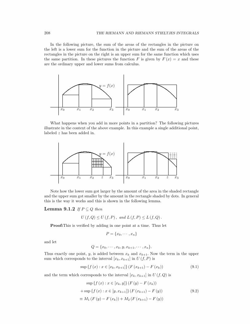
208 THE RIEMANN AND RIEMANN STIELTJES INTEGRALS
In the following picture, the sum of the areas of the rectangles in the picture onthe left is a lower sum for the function in the picture and the sum of the areas of therectangles in the picture on the right is an upper sum for the same function which usesthe same partition. In these pictures the function F is given by F (x) = x and theseare the ordinary upper and lower sums from calculus.
y = f(x)
x0 x1 x2 x3 x0 x1 x2 x3
What happens when you add in more points in a partition? The following picturesillustrate in the context of the above example. In this example a single additional point,labeled z has been added in.
y = f(x)
x0 x1 x2 x3z x0 x1 x2 x3z
Note how the lower sum got larger by the amount of the area in the shaded rectangleand the upper sum got smaller by the amount in the rectangle shaded by dots. In generalthis is the way it works and this is shown in the following lemma.
Lemma 9.1.2 If P ⊆ Q then
U (f,Q) ≤ U (f, P ) , and L (f, P ) ≤ L (f,Q) .
Proof:This is verified by adding in one point at a time. Thus let
P = {x0, · · · , xn}
and letQ = {x0, · · · , xk, y, xk+1, · · · , xn}.
Thus exactly one point, y, is added between xk and xk+1. Now the term in the uppersum which corresponds to the interval [xk, xk+1] in U (f, P ) is
sup {f (x) : x ∈ [xk, xk+1]} (F (xk+1)− F (xk)) (9.1)
and the term which corresponds to the interval [xk, xk+1] in U (f,Q) is
sup {f (x) : x ∈ [xk, y]} (F (y)− F (xk))
+ sup {f (x) : x ∈ [y, xk+1]} (F (xk+1)− F (y))
≡M1 (F (y)− F (xk)) +M2 (F (xk+1)− F (y))
(9.2)

9.1. THE DARBOUX STIELTJES INTEGRAL 209
All the other terms in the two sums coincide. Now sup {f (x) : x ∈ [xk, xk+1]} ≥max (M1,M2) and so the expression in 9.2 is no larger than
sup {f (x) : x ∈ [xk, xk+1]} (F (xk+1)− F (y))
+ sup {f (x) : x ∈ [xk, xk+1]} (F (y)− F (xk))
= sup {f (x) : x ∈ [xk, xk+1]} (F (xk+1)− F (xk)) ,
the term corresponding to the interval, [xk, xk+1] and U (f, P ) . This proves the firstpart of the lemma pertaining to upper sums because if Q ⊇ P, one can obtain Q fromP by adding in one point at a time and each time a point is added, the correspondingupper sum either gets smaller or stays the same. The second part about lower sums issimilar and is left as an exercise.
Lemma 9.1.3 If P and Q are two partitions, then
L (f, P ) ≤ U (f,Q) .
Proof:By Lemma 9.1.2,
L (f, P ) ≤ L (f, P ∪Q) ≤ U (f, P ∪Q) ≤ U (f,Q) .
Definition 9.1.4
I ≡ inf{U (f,Q) where Q is a partition}
I ≡ sup{L (f, P ) where P is a partition}.
Note that I and I are well defined real numbers.
Theorem 9.1.5 I ≤ I.
Proof:From Lemma 9.1.3,
I = sup{L (f, P ) where P is a partition} ≤ U (f,Q)
because U (f,Q) is an upper bound to the set of all lower sums and so it is no smallerthan the least upper bound. Therefore, since Q is arbitrary,
I = sup{L (f, P ) where P is a partition}≤ inf{U (f,Q) where Q is a partition} ≡ I
where the inequality holds because it was just shown that I is a lower bound to the setof all upper sums and so it is no larger than the greatest lower bound of this set. Thisproves the theorem.
Definition 9.1.6 A bounded function f is Darboux Stieltjes integrable, writtenas
f ∈ R ([a, b])
ifI = I
and in this case, ∫ b
a
f (x) dF ≡ I = I.
When F (x) = x, the integral is called the Darboux integral and is written as∫ b
a
f (x) dx.
210 THE RIEMANN AND RIEMANN STIELTJES INTEGRALS
Thus, in words, the Darboux integral is the unique number which lies between allupper sums and all lower sums if there is such a unique number.
Recall the following Proposition which comes from the definitions.
Proposition 9.1.7 Let S be a nonempty set and suppose −∞ < sup (S) < ∞.Then for every δ > 0,
S ∩ (sup (S)− δ, sup (S)] = ∅.
If inf (S) exists, then for every δ > 0,
S ∩ [inf (S) , inf (S) + δ) = ∅.
This proposition implies the following theorem which is used to determine the ques-tion of Darboux Stieltjes integrability.
Theorem 9.1.8 A bounded function f is Darboux Stieltjes integrable if and onlyif for all ε > 0, there exists a partition P such that
U (f, P )− L (f, P ) < ε. (9.3)
Proof:First assume f is Darboux Stieltjes integrable. Then let P and Q be twopartitions such that
U (f,Q) < I + ε/2, L (f, P ) > I − ε/2.
Then since I = I,
U (f,Q ∪ P )− L (f, P ∪Q) ≤ U (f,Q)− L (f, P ) < I + ε/2− (I − ε/2) = ε.
Now suppose that for all ε > 0 there exists a partition such that 9.3 holds. Then forgiven ε and partition P corresponding to ε
I − I ≤ U (f, P )− L (f, P ) ≤ ε.
Since ε is arbitrary, this shows I = I and this proves the theorem.The criterion of the above theorem which is equivalent to the existence of the Dar-
boux Stieltjes integral will be referred to in what follows as the Riemann criterion.Not all bounded functions are Darboux integrable. For example, let F (x) = x and
f (x) ≡{
1 if x ∈ Q0 if x ∈ R \Q (9.4)
Then if [a, b] = [0, 1] all upper sums for f equal 1 while all lower sums for f equal 0.Therefore the criterion of Theorem 9.1.8 is violated for ε = 1/2.
Here is an interesting theorem about change of variables [30]. First here is somenotation: f ∈ R [a, b;F ] will mean f is Darboux Stieltjes integrable on [a, b] and F isthe integrator. Also let
Mi (f) ≡ sup {f (x) : x ∈ [xi−1, xi]}
withmi (f) ≡ inf {f (x) : x ∈ [xi−1, xi]}
Theorem 9.1.9 Suppose ϕ is an increasing one to one and continuous functionwhich maps [a, b] onto [A,B] and f ∈ R [A,B;F ] . Then f ◦ ϕ ∈ R [a, b;F ◦ ϕ] and∫ b
a
f ◦ ϕd (F ◦ ϕ) =∫ B
A
fdF

9.2. EXERCISES 211
Proof: By assumption, there exists a partition of [A,B] , P = {y0, y1, · · · , yn} suchthat
ε > |U (P, f)− L (P, f)| (9.5)
Now let yi = ϕ (xi) so that {x0, x1, · · · , xn} is a partition of [a, b] , denoted by ϕ−1 (P ) .Also note
Mi (f) =Mi (f ◦ ϕ) , mi (f) = mi (f ◦ ϕ)
and
n∑i=1
Mi (f) (F (yi)− F (yi−1)) =n∑
i=1
Mi (f ◦ ϕ) (F (ϕ (xi))− F (ϕ (xi−1)))
with a similar conclusion holding for the lower sums. Then from 9.5,
ε > |U (P, f)− L (P, f)| =n∑
i=1
(Mi (f)−mi (f)) (F (yi)− F (yi−1))
=n∑
i=1
(Mi (f ◦ ϕ)−mi (f ◦ ϕ)) (F (ϕ (xi))− F (ϕ (xi−1)))
=∣∣U (ϕ−1 (P ) , f ◦ ϕ
)− L
(ϕ−1 (P ) , f ◦ ϕ
)∣∣which shows by the Riemann criterion that f ◦ ϕ ∈ R [a, b;F ◦ ϕ] . Also both∫ b
a
f ◦ ϕd (F ◦ ϕ) ,∫ B
A
fdF
are in the same interval of length ε,[L(ϕ−1 (P ) , f ◦ ϕ
), U(ϕ−1 (P ) , f ◦ ϕ
)]and so since ε is arbitrary, this shows the two integrals are the same. This proves thetheorem.
9.2 Exercises
1. Prove the second half of Lemma 9.1.2 about lower sums.
2. Verify that for f given in 9.4, the lower sums on the interval [0, 1] are all equal tozero while the upper sums are all equal to one.
3. Let f (x) = 1 + x2 for x ∈ [−1, 3] and let P ={−1,−1
3 , 0,12 , 1, 2
}. Find U (f, P )
and L (f, P ) for F (x) = x and for F (x) = x3.
4. Show that if f ∈ R ([a, b]) for F (x) = x, there exists a partition, {x0, · · · , xn}such that for any zk ∈ [xk, xk+1] ,∣∣∣∣∣
∫ b
a
f (x) dx−n∑
k=1
f (zk) (xk − xk−1)
∣∣∣∣∣ < ε
This sum,∑n
k=1 f (zk) (xk − xk−1) , is called a Riemann sum and this exerciseshows that the Darboux integral can always be approximated by a Riemann sum.For the general Darboux Stieltjes case, does anything change? Explain.

212 THE RIEMANN AND RIEMANN STIELTJES INTEGRALS
5. Suppose {fn} is a sequence of functions which are Darboux Stieltjes integrablewith respect to the integrator F on [a, b] . Suppose also that the sequence convergesuniformly to f on [a, b] . Show f is also integrable and
limn→∞
∫ b
a
fndF =
∫ b
a
fdF.
6. Let P ={1, 11
4 , 112 , 1
34 , 2}
and F (x) = x. Find upper and lower sums for thefunction f (x) = 1
x using this partition. What does this tell you about ln (2)?
7. If f ∈ R ([a, b]) with F (x) = x and f is changed at finitely many points, show thenew function is also in R ([a, b]) . Is this still true for the general case where F isonly assumed to be an increasing function? Explain.
8. In the case where F (x) = x, define a “left sum” as
n∑k=1
f (xk−1) (xk − xk−1)
and a “right sum”,n∑
k=1
f (xk) (xk − xk−1) .
Also suppose that all partitions have the property that xk−xk−1 equals a constant,(b− a) /n so the points in the partition are equally spaced, and define the integralto be the number these right and left sums get close to as n gets larger and larger.Show that for f given in 9.4,
∫ x
0f (t) dt = 1 if x is rational and
∫ x
0f (t) dt = 0
if x is irrational. It turns out that the correct answer should always equal zerofor that function, regardless of whether x is rational. This illustrates why thismethod of defining the integral in terms of left and right sums is total nonsense.Show that even though this is the case, it makes no difference if f is continuous.
9. The Darboux Stieltjes integral has been defined above for F an increasing in-tegrator function. Suppose F is an arbitrary function defined on [a, b] . ForPx ≡ {x0, · · · , xn} a partition of [a, x] ,define V (Px, F ) by
n∑i=1
|F (xi)− F (xi−1)| .
Define the total variation of F on [a, x] by
V[a,x] (F ) ≡ sup {V (Px, F ) : Px is a partition of [a, x]} .
Show x → V[a,x] (F ) is an increasing function. Then F is said to be of boundedvariation on [a, b] if V[a,b] (F ) is finite. Show that every function of boundedvariation can be written as the difference of two increasing functions one of whichis the function x→ V[a,x] (F ) .
10. Using Problem 9, explain how to define∫ b
afdF for F a function of bounded
variation.
11. The function F (x) ≡ ⌊x⌋ gives the greatest integer less than or equal to x. ThusF (1/2) = 0, F (5.67) = 5, F (5) = 5, etc. If F (x) = ⌊x⌋ as just described, find∫ 10
0xdF. More generally, find
∫ n
0f (x) dF where f is a continuous function.
12. Suppose f is a bounded function on [0, 1] and for each ε > 0, f is Darboux inte-grable on [ε, 1] . Can you conclude f is Darboux integrable on [0, 1]?
9.2. EXERCISES 213
9.2.1 Functions Of Darboux Integrable Functions
It is often necessary to consider functions of Darboux integrable functions and a naturalquestion is whether these are Darboux integrable. The following theorem gives a partialanswer to this question. This is not the most general theorem which will relate to thisquestion but it will be enough for the needs of this book.
Theorem 9.2.1 Let f, g be bounded functions and let
f ([a, b]) ⊆ [c1, d1] , g ([a, b]) ⊆ [c2, d2] .
Let H : [c1, d1]× [c2, d2]→ R satisfy,
|H (a1, b1)−H (a2, b2)| ≤ K [|a1 − a2|+ |b1 − b2|]
for some constant K. Then if f, g ∈ R ([a, b]) it follows that H ◦ (f, g) ∈ R ([a, b]) .
Proof: In the following claim, Mi (h) and mi (h) have the meanings assigned abovewith respect to some partition of [a, b] for the function h.
Claim: The following inequality holds.
|Mi (H ◦ (f, g))−mi (H ◦ (f, g))| ≤
K [|Mi (f)−mi (f)|+ |Mi (g)−mi (g)|] .Proof of the claim: By the above proposition, there exist x1, x2 ∈ [xi−1, xi] such
thatH (f (x1) , g (x1)) + η > Mi (H ◦ (f, g)) ,
andH (f (x2) , g (x2))− η < mi (H ◦ (f, g)) .
Then|Mi (H ◦ (f, g))−mi (H ◦ (f, g))|
< 2η + |H (f (x1) , g (x1))−H (f (x2) , g (x2))|< 2η +K [|f (x1)− f (x2)|+ |g (x1)− g (x2)|]≤ 2η +K [|Mi (f)−mi (f)|+ |Mi (g)−mi (g)|] .
Since η > 0 is arbitrary, this proves the claim.Now continuing with the proof of the theorem, let P be such that
n∑i=1
(Mi (f)−mi (f))∆Fi <ε
2K,
n∑i=1
(Mi (g)−mi (g))∆Fi <ε
2K.
Then from the claim,
n∑i=1
(Mi (H ◦ (f, g))−mi (H ◦ (f, g)))∆Fi
<n∑
i=1
K [|Mi (f)−mi (f)|+ |Mi (g)−mi (g)|]∆Fi < ε.
Since ε > 0 is arbitrary, this shows H ◦ (f, g) satisfies the Riemann criterion and henceH ◦ (f, g) is Darboux integrable as claimed. This proves the theorem.
This theorem implies that if f, g are Darboux Stieltjes integrable, then so is af +bg, |f | , f2, along with infinitely many other such continuous combinations of DarbouxStieltjes integrable functions. For example, to see that |f | is Darboux integrable, letH (a, b) = |a| . Clearly this function satisfies the conditions of the above theorem and so|f | = H (f, f) ∈ R ([a, b]) as claimed. The following theorem gives an example of manyfunctions which are Darboux Stieltjes integrable.

214 THE RIEMANN AND RIEMANN STIELTJES INTEGRALS
Theorem 9.2.2 Let f : [a, b] → R be either increasing or decreasing on [a, b]and suppose F is continuous. Then f ∈ R ([a, b]) . If f : [a, b] → R is either increasingor decreasing and continuous and no continuity requirement is made on F then f ∈R ([a, b]).
Proof:Let ε > 0 be given and let
xi = a+ i
(b− an
), i = 0, · · · , n.
Since F is continuous, it follows from Corollary 6.8.3 on Page 117, it is uniformlycontinuous. Therefore, if n is large enough, then for all i,
F (xi)− F (xi−1) <ε
f (b)− f (a) + 1
Then since f is increasing,
U (f, P )− L (f, P ) =n∑
i=1
(f (xi)− f (xi−1)) (F (xi)− F (xi−1))
≤ ε
f (b)− f (a) + 1
n∑i=1
(f (xi)− f (xi−1))
=ε
f (b)− f (a) + 1(f (b)− f (a)) < ε.
Thus the Riemann criterion is satisfied and so the function is Darboux Stieltjes inte-grable. The proof for decreasing f is similar.
Now consider the case where f is continuous and increasing and F is only given tobe increasing. Then as before, if P is a partition, {x0, · · · , xn} ,
U (f, P )− L (f, P ) =n∑
i=1
(f (xi)− f (xi−1)) (F (xi)− F (xi−1)) (9.6)
Since f is continuous, it is uniformly continuous and so there exists δ > 0 such that if|x− y| < δ, then
|f (x)− f (y)| < ε
(F (b)− F (a)) + 1
Then in 9.6, if each |xi − xi−1| < δ, then
U (f, P )− L (f, P ) ≤n∑
i=1
ε
(F (b)− F (a)) + 1(F (xi)− F (xi−1))
≤ ε
(F (b)− F (a)) + 1(F (b)− F (a)) < ε
Thus the Riemann criterion is satisfied and so the function is Darboux Stieltjes inte-grable. The proof for decreasing f is similar. This proves the theorem.
Corollary 9.2.3 Let [a, b] be a bounded closed interval and let ϕ : [a, b] → R beLipschitz continuous and suppose F is increasing. Then ϕ ∈ R ([a, b]) . Recall that afunction ϕ, is Lipschitz continuous if there is a constant, K, such that for all x, y,
|ϕ (x)− ϕ (y)| < K |x− y| .

9.2. EXERCISES 215
Proof:Let f (x) = x. Then by Theorem 9.2.2, f is Darboux Stieltjes integrable. LetH (a, b) ≡ ϕ (a). Then by Theorem 9.2.1 H ◦ (f, f) = ϕ◦f = ϕ is also Darboux Stieltjesintegrable. This proves the corollary.
In fact, it is enough to assume ϕ is continuous, although this is harder. This is thecontent of the next theorem which is where the difficult theorems about continuity anduniform continuity are used.
Theorem 9.2.4 Suppose f : [a, b]→ R is continuous and F is just an increasingfunction defined on [a, b]. Then f ∈ R ([a, b]) .
Proof:By Corollary 6.8.3 on Page 117, f is uniformly continuous on [a, b] . Therefore,if ε > 0 is given, there exists a δ > 0 such that if |xi − xi−1| < δ, then Mi − mi <
εF (b)−F (a)+1 . Let
P ≡ {x0, · · · , xn}
be a partition with |xi − xi−1| < δ. Then
U (f, P )− L (f, P ) <n∑
i=1
(Mi −mi) (F (xi)− F (xi−1))
<ε
F (b)− F (a) + 1(F (b)− F (a)) < ε.
By the Riemann criterion, f ∈ R ([a, b]) . This proves the theorem.
9.2.2 Properties Of The Integral
The integral has many important algebraic properties. First here is a simple lemma.
Lemma 9.2.5 Let S be a nonempty set which is bounded above and below. Then if−S ≡ {−x : x ∈ S} ,
sup (−S) = − inf (S) (9.7)
and
inf (−S) = − sup (S) . (9.8)
Proof: Consider 9.7. Let x ∈ S. Then −x ≤ sup (−S) and so x ≥ − sup (−S) .If follows that − sup (−S) is a lower bound for S and therefore, − sup (−S) ≤ inf (S) .This implies sup (−S) ≥ − inf (S) . Now let −x ∈ −S. Then x ∈ S and so x ≥ inf (S)which implies −x ≤ − inf (S) . Therefore, − inf (S) is an upper bound for −S and so− inf (S) ≥ sup (−S) . This shows 9.7. Formula 9.8 is similar and is left as an exercise.
In particular, the above lemma implies that for Mi (f) and mi (f) defined aboveMi (−f) = −mi (f) , and mi (−f) = −Mi (f) .
Lemma 9.2.6 If f ∈ R ([a, b]) then −f ∈ R ([a, b]) and
−∫ b
a
f (x) dF =
∫ b
a
−f (x) dF.
Proof: The first part of the conclusion of this lemma follows from Theorem 9.2.2since the function ϕ (y) ≡ −y is Lipschitz continuous. Now choose P such that∫ b
a
−f (x) dF − L (−f, P ) < ε.
216 THE RIEMANN AND RIEMANN STIELTJES INTEGRALS
Then since mi (−f) = −Mi (f) ,
ε >
∫ b
a
−f (x) dF −n∑
i=1
mi (−f)∆Fi =
∫ b
a
−f (x) dF +n∑
i=1
Mi (f)∆Fi
which implies
ε >
∫ b
a
−f (x) dF +n∑
i=1
Mi (f)∆Fi ≥∫ b
a
−f (x) dF +
∫ b
a
f (x) dF.
Thus, since ε is arbitrary, ∫ b
a
−f (x) dF ≤ −∫ b
a
f (x) dF
whenever f ∈ R ([a, b]) . It follows∫ b
a
−f (x) dF ≤ −∫ b
a
f (x) dF = −∫ b
a
− (−f (x)) dF ≤∫ b
a
−f (x) dF
and this proves the lemma.
Theorem 9.2.7 The integral is linear,∫ b
a
(αf + βg) (x) dF = α
∫ b
a
f (x) dF + β
∫ b
a
g (x) dF.
whenever f, g ∈ R ([a, b]) and α, β ∈ R.
Proof: First note that by Theorem 9.2.1, αf + βg ∈ R ([a, b]) . To begin with,consider the claim that if f, g ∈ R ([a, b]) then∫ b
a
(f + g) (x) dF =
∫ b
a
f (x) dF +
∫ b
a
g (x) dF. (9.9)
Let P1,Q1 be such that
U (f,Q1)− L (f,Q1) < ε/2, U (g, P1)− L (g, P1) < ε/2.
Then letting P ≡ P1 ∪Q1, Lemma 9.1.2 implies
U (f, P )− L (f, P ) < ε/2, and U (g, P )− U (g, P ) < ε/2.
Next note that
mi (f + g) ≥ mi (f) +mi (g) , Mi (f + g) ≤Mi (f) +Mi (g) .
Therefore,
L (g + f, P ) ≥ L (f, P ) + L (g, P ) , U (g + f, P ) ≤ U (f, P ) + U (g, P ) .
For this partition,∫ b
a
(f + g) (x) dF ∈ [L (f + g, P ) , U (f + g, P )]
⊆ [L (f, P ) + L (g, P ) , U (f, P ) + U (g, P )]

9.2. EXERCISES 217
and ∫ b
a
f (x) dF +
∫ b
a
g (x) dF ∈ [L (f, P ) + L (g, P ) , U (f, P ) + U (g, P )] .
Therefore, ∣∣∣∣∣∫ b
a
(f + g) (x) dF −
(∫ b
a
f (x) dF +
∫ b
a
g (x) dF
)∣∣∣∣∣ ≤U (f, P ) + U (g, P )− (L (f, P ) + L (g, P )) < ε/2 + ε/2 = ε.
This proves 9.9 since ε is arbitrary.It remains to show that
α
∫ b
a
f (x) dF =
∫ b
a
αf (x) dF.
Suppose first that α ≥ 0. Then∫ b
a
αf (x) dF ≡ sup{L (αf, P ) : P is a partition} =
α sup{L (f, P ) : P is a partition} ≡ α∫ b
a
f (x) dF.
If α < 0, then this and Lemma 9.2.6 imply∫ b
a
αf (x) dF =
∫ b
a
(−α) (−f (x)) dF
= (−α)∫ b
a
(−f (x)) dF = α
∫ b
a
f (x) dF.
This proves the theorem.In the next theorem, suppose F is defined on [a, b] ∪ [b, c] .
Theorem 9.2.8 If f ∈ R ([a, b]) and f ∈ R ([b, c]) , then f ∈ R ([a, c]) and∫ c
a
f (x) dF =
∫ b
a
f (x) dF +
∫ c
b
f (x) dF. (9.10)
Proof: Let P1 be a partition of [a, b] and P2 be a partition of [b, c] such that
U (f, Pi)− L (f, Pi) < ε/2, i = 1, 2.
Let P ≡ P1 ∪ P2. Then P is a partition of [a, c] and
U (f, P )− L (f, P )
= U (f, P1)− L (f, P1) + U (f, P2)− L (f, P2) < ε/2 + ε/2 = ε. (9.11)
Thus, f ∈ R ([a, c]) by the Riemann criterion and also for this partition,∫ b
a
f (x) dF +
∫ c
b
f (x) dF ∈ [L (f, P1) + L (f, P2) , U (f, P1) + U (f, P2)]
= [L (f, P ) , U (f, P )]

218 THE RIEMANN AND RIEMANN STIELTJES INTEGRALS
and ∫ c
a
f (x) dF ∈ [L (f, P ) , U (f, P )] .
Hence by 9.11,∣∣∣∣∣∫ c
a
f (x) dF −
(∫ b
a
f (x) dF +
∫ c
b
f (x) dF
)∣∣∣∣∣ < U (f, P )− L (f, P ) < ε
which shows that since ε is arbitrary, 9.10 holds. This proves the theorem.
Corollary 9.2.9 Let F be continuous and let [a, b] be a closed and bounded intervaland suppose that
a = y1 < y2 · · · < yl = b
and that f is a bounded function defined on [a, b] which has the property that f iseither increasing on [yj , yj+1] or decreasing on [yj , yj+1] for j = 1, · · · , l − 1. Then f∈ R ([a, b]) .
Proof:This follows from Theorem 9.2.8 and Theorem 9.2.2.Given this corollary, can you think of functions which do not satisfy the conditions of
this corollary? They certainly exist. Think of the one which was 1 on the rationals and0 on the irrationals. This is a sick function and that is what is needed for the Darbouxintegral to not exist. Unfortunately, sometimes sick functions cannot be avoided.
The symbol,∫ b
af (x) dF when a > b has not yet been defined.
Definition 9.2.10 Let [a, b] be an interval and let f ∈ R ([a, b]) . Then∫ a
b
f (x) dF ≡ −∫ b
a
f (x) dF.
Note that with this definition,∫ a
a
f (x) dF = −∫ a
a
f (x) dF
and so ∫ a
a
f (x) dF = 0.
Theorem 9.2.11 Assuming all the integrals make sense,∫ b
a
f (x) dF +
∫ c
b
f (x) dF =
∫ c
a
f (x) dF.
Proof:This follows from Theorem 9.2.8 and Definition 9.2.10. For example, assume
c ∈ (a, b) .
Then from Theorem 9.2.8,∫ c
a
f (x) dF +
∫ b
c
f (x) dF =
∫ b
a
f (x) dF
and so by Definition 9.2.10,∫ c
a
f (x) dF =
∫ b
a
f (x) dF −∫ b
c
f (x) dF
=
∫ b
a
f (x) dF +
∫ c
b
f (x) dF.

9.2. EXERCISES 219
The other cases are similar.The following properties of the integral have either been established or they follow
quickly from what has been shown so far.
If f ∈ R ([a, b]) then if c ∈ [a, b] , f ∈ R ([a, c]) , (9.12)∫ b
a
αdF = α (F (b)− F (a)) , (9.13)
∫ b
a
(αf + βg) (x) dF = α
∫ b
a
f (x) dF + β
∫ b
a
g (x) dF, (9.14)
∫ b
a
f (x) dF +
∫ c
b
f (x) dF =
∫ c
a
f (x) dF, (9.15)
∫ b
a
f (x) dF ≥ 0 if f (x) ≥ 0 and a < b, (9.16)∣∣∣∣∣∫ b
a
f (x) dF
∣∣∣∣∣ ≤∣∣∣∣∣∫ b
a
|f (x)| dF
∣∣∣∣∣ . (9.17)
The only one of these claims which may not be completely obvious is the last one. Toshow this one, note that
|f (x)| − f (x) ≥ 0, |f (x)|+ f (x) ≥ 0.
Therefore, by 9.16 and 9.14, if a < b,∫ b
a
|f (x)| dF ≥∫ b
a
f (x) dF
and ∫ b
a
|f (x)| dF ≥ −∫ b
a
f (x) dF.
Therefore, ∫ b
a
|f (x)| dF ≥
∣∣∣∣∣∫ b
a
f (x) dF
∣∣∣∣∣ .If b < a then the above inequality holds with a and b switched. This implies 9.17.
9.2.3 Fundamental Theorem Of Calculus
In this section F (x) = x so things are specialized to the ordinary Darboux integral.With these properties 9.12 - 9.17, it is easy to prove the fundamental theorem of cal-culus2. Let f ∈ R ([a, b]) . Then by 9.12 f ∈ R ([a, x]) for each x ∈ [a, b] . The firstversion of the fundamental theorem of calculus is a statement about the derivative ofthe function
x→∫ x
a
f (t) dt.
2This theorem is why Newton and Liebnitz are credited with inventing calculus. The integral hadbeen around for thousands of years and the derivative was by their time well known. However theconnection between these two ideas had not been fully made although Newton’s predecessor, IsaacBarrow had made some progress in this direction.

220 THE RIEMANN AND RIEMANN STIELTJES INTEGRALS
Theorem 9.2.12 Let f ∈ R ([a, b]) and let
F (x) ≡∫ x
a
f (t) dt.
Then if f is continuous at x ∈ [a, b] ,
F ′ (x) = f (x)
where the derivative refers to the right or left derivative at the endpoints.
Proof:Let x ∈ [a, b] be a point of continuity of f and let h be small enough thatx+ h ∈ [a, b] . Then by using 9.15,
F (x+ h)− F (x)− f (x)h
= F (x+ h)− F (x)−∫ x+h
x
f (t) dt+
(∫ x+h
x
f (t) dt− f (x)h
)
=
∫ x+h
x
f (t) dt− f (x)h
I need to verify ∫ x+h
x
f (t) dt− f (x)h = o (h) .
Using 9.13,
f (x) = h−1
∫ x+h
x
f (x) dt.
Therefore, by 9.17,∣∣∣∣∣ 1h(∫ x+h
x
f (t) dt− f (x)h
)∣∣∣∣∣ =∣∣∣∣∣h−1
∫ x+h
x
(f (t)− f (x)) dt
∣∣∣∣∣≤
∣∣∣∣∣h−1
∫ x+h
x
|f (t)− f (x)| dt
∣∣∣∣∣ .Let ε > 0 and let δ > 0 be small enough that if |t− x| < δ, then
|f (t)− f (x)| < ε.
Therefore, if |h| < δ, the above inequality and 9.13 shows that∣∣h−1 (F (x+ h)− F (x))− f (x)∣∣ ≤ |h|−1
ε |h| = ε.
Since ε > 0 is arbitrary, this shows∫ x+h
x
f (t) dt− f (x)h = o (h)
and so this proves the theorem.Note this gives existence of a function G which is a solution to the initial value
problem,G′ (x) = f (x) , G (a) = 0
whenever f is continuous. This is because of Theorem 9.2.4 which gives the existenceof the integral of a continuous function.
The next theorem is also called the fundamental theorem of calculus.

9.2. EXERCISES 221
Theorem 9.2.13 Let f ∈ R ([a, b]) and suppose G′ (x) = f (x) at every point of(a, b) and G is continuous on [a, b] . Then∫ b
a
f (x) dx = G (b)−G (a) . (9.18)
Proof:Let P = {x0, · · · , xn} be a partition satisfying
U (f, P )− L (f, P ) < ε.
Then
G (b)−G (a) = G (xn)−G (x0)
=n∑
i=1
G (xi)−G (xi−1) .
By the mean value theorem,
G (b)−G (a) =n∑
i=1
G′ (zi) (xi − xi−1)
=
n∑i=1
f (zi)∆xi
where zi is some point in (xi−1, xi) . It follows, since the above sum lies between theupper and lower sums, that
G (b)−G (a) ∈ [L (f, P ) , U (f, P )] ,
and also ∫ b
a
f (x) dx ∈ [L (f, P ) , U (f, P )] .
Therefore, ∣∣∣∣∣G (b)−G (a)−∫ b
a
f (x) dx
∣∣∣∣∣ < U (f, P )− L (f, P ) < ε.
Since ε > 0 is arbitrary, 9.18 holds. This proves the theorem.The following notation is often used in this context. Suppose F is an antiderivative
of f as just described with F continuous on [a, b] and F ′ = f on (a, b) . Then∫ b
a
f (x) dx = F (b)− F (a) ≡ F (x) |ba.
Definition 9.2.14 Let f be a bounded function defined on a closed interval[a, b] and let P ≡ {x0, · · · , xn} be a partition of the interval. Suppose zi ∈ [xi−1, xi] ischosen. Then the sum
n∑i=1
f (zi) (xi − xi−1)
is known as a Riemann sum. Also,
||P || ≡ max {|xi − xi−1| : i = 1, · · · , n} . (9.19)

222 THE RIEMANN AND RIEMANN STIELTJES INTEGRALS
Proposition 9.2.15 Suppose f ∈ R ([a, b]) . Then there exists a partition, P ≡{x0, · · · , xn} with the property that for any choice of zk ∈ [xk−1, xk] ,∣∣∣∣∣
∫ b
a
f (x) dx−n∑
k=1
f (zk) (xk − xk−1)
∣∣∣∣∣ < ε.
Proof: Choose P such that U (f, P ) − L (f, P ) < ε and then both∫ b
af (x) dx
and∑n
k=1 f (zk) (xk − xk−1) are contained in [L (f, P ) , U (f, P )] and so the claimedinequality must hold. This proves the proposition.
You should think how the above proposition would change in the more general caseof a Darboux Stieltjes integral. This proposition is significant because it gives a way ofapproximating the integral.
9.3 Exercises
1. Suppose {fn} is a sequence of Darboux Stieltjes integrable functions defined on aclosed interval, [a, b] . Suppose fn → f uniformly on [a, b] . Show
limn→∞
∫ b
a
fndF =
∫ b
a
fdF.
Included in showing this is the verification that f is Darboux Stieltjes integrable.
2. Let f, g be bounded functions and let
f ([a, b]) ⊆ [c1, d1] , g ([a, b]) ⊆ [c2, d2] .
Let H : [c1, d1]× [c2, d2]→ R satisfy, the following condition at every point (x, y).For every ε > 0 there exists a δ > 0 such that if
(x, y) , (x1, y1) ∈ [c1, d1]× [c2, d2]
and max (|x− x1| , |y − y1|) < δ then
|H (x, y)−H (x1, y1)| < ε
Then if f, g ∈ R ([a, b]) it follows that H ◦ (f, g) ∈ R ([a, b]) . Is the foregoingstatement true? Prove or disprove.
3. A differentiable function f defined on (0,∞) satisfies the following conditions.
f (xy) = f (x) + f (y) , f ′ (1) = 1.
Find f and sketch its graph.
4. Does there exist a function which has two continuous derivatives but the thirdderivative fails to exist at any point? If so, give an example. If not, explain why.
5. Suppose f is a continuous function on [a, b] and∫ b
a
f2dF = 0.
where F is a strictly increasing integrator function. Show that then f (x) = 0 forall x. If F is not strictly increasing, is the result still true?

9.3. EXERCISES 223
6. Suppose f is a continuous function and∫ b
a
f (x)xndx = 0
for n = 0, 1, 2, 3 · · · . Show using Problem 5 that f (x) = 0 for all x. Hint: Youmight use the Weierstrass approximation theorem.
7. Here is a function:
f (x) =
{x2 sin
(1x2
)if x = 0
0 if x = 0
Show this function has a derivative at every point of R. Does it make any senseto write ∫ 1
0
f ′ (x) dx = f (1)− f (0) = f (1)?
Explain.
8. Let
f (x) =
{sin(1x
)if x = 0
0 if x = 0
Is f Darboux integrable with respect to the integrator F (x) = x on the interval[0, 1]?
9. Recall that for a power series,
∞∑k=0
ak (x− c)k
you could differentiate term by term on the interval of convergence. Show that ifthe radius of convergence of the above series is r > 0 and if [a, b] ⊆ (c− r, c+ r) ,then ∫ b
a
∞∑k=0
ak (x− c)k dx
= a0 (b− a) +∞∑k=1
akk
(b− c)k+1 −∞∑k=1
akk
(a− c)k+1
In other words, you can integrate term by term.
10. Find∑∞
k=12−k
k .
11. Let f be Darboux integrable on [0, 1] . Show x→∫ x
0f (t) dt is continuous.
12. Suppose f, g are two functions which are continuous with continuous derivativeson [a, b] . Show using the fundamental theorem of calculus and the product rulethe integration by parts formula. Also explain why all the terms make sense.∫ b
a
f ′ (t) g (t) dt = f (b) g (b)− f (a) g (a)−∫ b
a
f (t) g′ (t) dt
13. Show1
1 + x2=
n∑k=0
(−1)k x2k +(−1)n+1
x2n+2
1 + x2.

224 THE RIEMANN AND RIEMANN STIELTJES INTEGRALS
Now use this to find a series which converges to arctan (1) = π/4. Recall
arctan (x) =
∫ x
0
1
1 + t2dt.
For which values of x will your series converge? For which values of x does theabove description of arctan in terms of an integral make sense? Does this help toshow the inferiority of power series?
14. Define F (x) ≡∫ x
01
1+t2 dt. Of course F (x) = arctan (x) as mentioned above butjust consider this function in terms of the integral. Sketch the graph of F usingonly its definition as an integral. Show there exists a constant M such that−M ≤ F (x) ≤ M. Next explain why limx→∞ F (x) exists and show this limitequals − limx→−∞ F (x).
15. In Problem 14 let the limit defined there be denoted by π/2 and define T (x) ≡F−1 (x) for x ∈ (−π/2, π/2) . Show T ′ (x) = 1 + T (x)
2and T (0) = 0. As
part of this, you must explain why T ′ (x) exists. For x ∈ [0, π/2] let C (x) ≡1/
√1 + T (x)
2with C (π/2) = 0 and on [0, π/2] , define S (x) by
√1− C (x)
2.
Show both S (x) and C (x) are differentiable on [0, π/2] and satisfy S′ (x) = C (x)and C ′ (x) = −S (x) . Find the appropriate way to define S (x) and C (x) on allof [0, 2π] in order that these functions will be sin (x) and cos (x) and then extendto make the result periodic of period 2π on all of R. Note this is a way to definethe trig. functions which is independent of plane geometry and also does not usepower series. See the book by Hardy, [18] for this approach.
16. Show
arcsin (x) =
∫ x
0
1√1− t2
dt.
Now use the binomial theorem to find a power series for arcsin (x) .
17. The initial value problem from ordinary differential equations is of the form
y′ = f (y) , y (0) = y0.
Suppose f is a continuous function of y. Show that a function t→ y (t) solves theabove initial value problem if and only if
y (t) = y0 +
∫ t
0
f (y (s)) ds.
18. Let p, q > 1 and satisfy1
p+
1
q= 1.
Consider the function x = tp−1. Then solving for t, you get t = x1/(p−1) = xq−1.Explain this. Now let a, b ≥ 0. Sketch a picture to show why∫ b
0
xq−1dx+
∫ a
0
tp−1dt ≥ ab.
Now do the integrals to obtain a very important inequality
bq
q+ap
p≥ ab.
When will equality hold in this inequality?

9.4. THE RIEMANN STIELTJES INTEGRAL 225
19. Suppose f, g are two Darboux integrable functions on [a, b] with respect to anintegrator F. Verify Holder’s inequality.
∫ b
a
|f | |g| dF ≤
(∫ b
a
|f |p dF
)1/p(∫ b
a
|g|q dF
)1/q
Hint: Do the following. Let A =(∫ b
a|f |p dF
)1/p, B =
(∫ b
a|g|q dF
)1/q. Then let
a =|f |A, b =
|g|B
and use the wonderful inequality of Problem 18.
9.4 The Riemann Stieltjes Integral
The definition of integrability given above is also called Darboux integrability and theintegral defined as the unique number which lies between all upper sums and all lowersums is called the Darboux integral . The definition of the Riemann integral in termsof Riemann sums is given next. I will show that these two integrals are often the samething.
Definition 9.4.1 A bounded function f defined on [a, b] is said to be RiemannStieltjes integrable if there exists a number, I with the property that for every ε > 0,there exists δ > 0 such that if
P ≡ {x0, x1, · · · , xn}
is any partition having ||P || < δ, and zi ∈ [xi−1, xi] ,∣∣∣∣∣I −n∑
i=1
f (zi) (F (xi)− F (xi−1))
∣∣∣∣∣ < ε.
The number∫ b
af (x) dF is defined as I.
It turns out Riemann Stieltjes and Darboux Stieltjes integrals are often the same.This was shown by Darboux. The Darboux integral is easier to understand and this iswhy it was presented first but the Riemann integral is the right way to look at it if youwant to generalize. The next theorem shows it is always at least as easy for a functionto be Darboux integrable as Riemann integrable.
Theorem 9.4.2 If a bounded function defined on [a, b] is Riemann Stieltjes inte-grable with respect to an increasing F in the sense of Definition 9.4.1 then it is DarbouxStieltjes integrable. Furthermore the two integrals coincide.
Proof: Let f be a bounded function integrable in the sense of Definition 9.4.1. Thisimplies there exists I and a partition
P = {x0, x1, · · · , xn}
such that whenever zi ∈ [xi−1, xi] ,∣∣∣∣∣I −n∑
i=1
f (zi) (F (xi)− F (xi−1))
∣∣∣∣∣ < ε/3
226 THE RIEMANN AND RIEMANN STIELTJES INTEGRALS
It follows that for Mi and mi defined as before,∣∣∣∣∣I −n∑
i=1
Mi (F (xi)− F (xi−1))
∣∣∣∣∣ ≤ ε/3∣∣∣∣∣I −
n∑i=1
mi (F (xi)− F (xi−1))
∣∣∣∣∣ ≤ ε/3Thus for this partition, P,
U (P, f)− L (P, f) =n∑
i=1
Mi (F (xi)− F (xi−1))−n∑
i=1
mi (F (xi)− F (xi−1))
=n∑
i=1
Mi (F (xi)− F (xi−1))− I +
(I −
n∑i=1
mi (F (xi)− F (xi−1))
)
≤
∣∣∣∣∣n∑
i=1
Mi (F (xi)− F (xi−1))− I
∣∣∣∣∣+∣∣∣∣∣I −
n∑i=1
mi (F (xi)− F (xi−1))
∣∣∣∣∣≤ ε
3+ε
3=
2ε
3< ε
Since ε is arbitrary, this and the Riemann criterion shows f is Darboux integrable.
It also follows I =∫ b
afdF where
∫ b
afdF is the Darboux integral because∣∣∣∣∣I −
∫ b
a
fdF
∣∣∣∣∣ ≤∣∣∣∣∣I −
n∑i=1
Mi (F (xi)− F (xi−1))
∣∣∣∣∣+
∣∣∣∣∣n∑
i=1
Mi (F (xi)− F (xi−1))−∫ b
a
fdF
∣∣∣∣∣≤ ε
3+
2ε
3= ε
and ε is arbitrary.
Is the converse true? If f is Darboux Stieltjes integrable, is it also Riemann Stieltjesintegrable in the sense of Definition 9.4.1? The answer is often yes. The theorem willbe proved using some lemmas.
Lemma 9.4.3 Suppose f is a bounded function defined on [a, b] and |f (x)| < M forall x ∈ [a, b] . Let Q be a partition having n points, {x∗0, · · · , x∗n} and let P be any otherpartition. Then
|U (f, P )− L (f, P )| ≤ 2Mn ||PF ||+ |U (f,Q)− L (f,Q)|
where ||PF || is defined by
max {F (xi)− F (xi−1) : P = {x0, · · · , xm}}
Proof of the lemma: Let P = {x0, · · · , xm} . Let I denote the set
I ≡ {i : [xi−1, xi] contains some point of Q}

9.4. THE RIEMANN STIELTJES INTEGRAL 227
and IC ≡ {0, · · · ,m} \ I. Then
U (f, P )− L (f, P ) =∑i∈I
(Mi −mi) (F (xi)− F (xi−1))
+∑i∈IC
(Mi −mi) (F (xi)− F (xi−1))
In the second sum above, for each i ∈ IC , [xi−1, xi] must be contained in[x∗k−1, x
∗k
]for
some k. Therefore, each term in this second sum is no larger than a corresponding termin the sum which equals U (f,Q)−L (f,Q) . Therefore, the second sum is no larger thanU (f,Q)− L (f,Q) . Now consider the first sum. Since |f (x)| ≤M,
(Mi −mi) (F (xi)− F (xi−1)) ≤ 2M ||PF ||
and so since each of these intervals [xi−1, xi] for i ∈ I contains at least one point of Q,there can be no more than n of these. Hence the first sum is dominated by
2Mn ||PF || .
This proves the lemma.
Lemma 9.4.4 If ε > 0 is given and f is a Darboux integrable function defined on[a, b], then there exists δ > 0 such that whenever ||PF || < δ, then
|U (f, P )− L (f, P )| < ε.
Proof of the lemma: Suppose Q is a partition such that U (f,Q)−L (f,Q) < ε/2.There exists such a partition because f is given to be Darboux integrable. Say Q hasn intervals. Then if P is any partition such that 2Mn ||PF || < ε/2, it follows from thepreceeding lemma that
|U (f, P )− L (f, P )| ≤ 2Mn ||PF ||+ |U (f,Q)− L (f,Q)|< ε/2 + ε/2 = ε.
This proves the lemma.
Theorem 9.4.5 Suppose f is Darboux Stieltjes integrable and the integrator, Fis increasing and continuous. Then f is Riemann Stieltjes integrable as described inDefinition 9.4.1.
Proof: By Lemma 9.4.4 there exists δ > 0 such that if ||PF || < δ, then
|U (f, P )− L (f, P )| < ε.
By the continuity of F, there exists η > 0 such that if ||P || < η, then ||PF || < δ. There-
fore, the above inequality holds for such P. Letting∫ b
afdF be the Darboux Stieltjes
integral, it follows that every Riemann Stieltjes sum corresponding to ||P || < δ has the
property that this sum is closer to∫ b
afdF than ε which shows f is Riemann Stieltjes
integrable in the sense of Definition 9.4.1 and I =∫ b
afdF. This proves the theorem.
Note this shows that the Riemann integral and the Darboux integral are completelyequivalent whenever the integrator function is continuous. This is the case when theintegrator function is F (x) = x which is the usual Riemann integral of calculus.
Recall that a continuous function f is Darboux Stieltjes integrable whenever theintegrator is increasing, not necessarily continuous. Does the same theorem hold forRiemann Stieltjes integrability in the sense of Definition 9.4.1? It does.

228 THE RIEMANN AND RIEMANN STIELTJES INTEGRALS
Theorem 9.4.6 Let f be continuous on [a, b]. Then f is Riemann Stieltjesintegrable in the sense of Definition 9.4.1.
Proof: Since f is continuous and [a, b] is sequentially compact, it follows fromTheorem 6.8.2 that f is uniformly continuous. Thus if ε > 0 is given, there exists δ > 0such that if |x− y| < δ, then
|f (x)− f (y)| < ε
2 (F (b)− F (a) + 1).
Let P = {x0, · · · , xn} be a partition such that ||P || < δ. Now if you add in a point zon the interior of Ij and consider the new partition,
x0 < · · · < xj−1 < z < xj < · · · < xn
denoting it by P ′,
S (P, f)− S (P ′, f) =
j−1∑i=1
(f (ti)− f (t′i)) (F (xi)− F (xi−1))
+f (tj) (F (xj)− F (xj−1))− f(t′j)(F (z)− F (xj−1))
−f(t′j+1
)(F (xj)− F (z)) +
n∑i=j+1
(f (ti)− f
(t′i+1
))(F (xi)− F (xi−1))
The term, f (tj) (F (xj)− F (xj−1)) can be written as
f (tj) (F (xj)− F (xj−1)) = f (tj) (F (xj)− F (z)) + f (tj) (F (z)− F (xj−1))
and so, the middle terms can be written as
f (tj) (F (xj)− F (z)) + f (tj) (F (z)− F (xj−1))
−f(t′j)(F (z)− F (xj−1))− f
(t′j+1
)(F (xj)− F (z))
=(f (tj)− f
(t′j+1
))(F (xj)− F (z))
+(f (tj)− f
(t′j))
(F (z)− F (xj−1))
The absolute value of this is dominated by
<ε
2 (F (b)− F (a) + 1)(F (xj)− F (xj−1))
This is because the various pairs of values at which f is evaluated are closer than δ.Similarly, ∣∣∣∣∣
j−1∑i=1
(f (ti)− f (t′i)) (F (xi)− F (xi−1))
∣∣∣∣∣≤
j−1∑i=1
|f (ti)− f (t′i)| (F (xi)− F (xi−1))
≤j−1∑i=1
ε
2 (F (b)− F (a) + 1)(F (xi)− F (xi−1))

9.4. THE RIEMANN STIELTJES INTEGRAL 229
and ∣∣∣∣∣∣n∑
i=j+1
(f (ti)− f
(t′i+1
))(F (xi)− F (xi−1))
∣∣∣∣∣∣≤
n∑i=j+1
ε
2 (F (b)− F (a) + 1)(F (xi)− F (xi−1)) .
Thus
|S (P, f)− S (P ′, f)| ≤n∑
i=1
ε
2 (F (b)− F (a) + 1)(F (xi)− F (xi−1)) < ε/2.
Similar reasoning would apply if you added in two new points in the partition or moregenerally, any finite number of new points. You would just have to consider moreexceptional terms. Therefore, if ||P || < δ and Q is any partition, then from what wasjust shown, you can pick the points on the interiors of the intervals any way you likeand
|S (P, f)− S (P ∪Q, f)| < ε/2.
Therefore, if ||P || , ||Q|| < δ,
|S (P, f)− S (Q, f)| ≤ |S (P, f)− S (P ∪Q, f)|+ |S (P ∪Q, f)− S (Q, f)|< ε/2 + ε/2 = ε
Now consider a sequence εn → 0. Then from what was just shown, there exist δn > 0such that for ||P || , ||Q|| < δn,
|S (P, f)− S (Q, f)| < εn
Let Kn be defined byKn ≡ ∪{S (P, f) : ||P || < δn}.
In other words, take the closure of the set of numbers consisting of all Riemann sums,S (P, f) such that ||P || < δn. It follows from the definition, Kn ⊇ Kn+1 for all n andeach Kn is closed with diam (Kn)→ 0. Then by Theorem 4.12.20 there exists a uniqueI ∈ ∩∞n=1Kn. Letting ε > 0, there exists n such that εn < ε. Then if ||P || < δn, itfollows |S (P, f)− I| ≤ εn < ε. Thus f is Riemann Stieltjes integrable in the sense of
Definition 9.4.1 and I =∫ b
afdF . This proves the theorem.
9.4.1 Change Of Variables
The formulation of the integral in terms of limits of Riemann sums makes it easy toestablish the following lemma and change of variables formula which is well known frombeginning calculus courses although there it is presented in less generality.
Lemma 9.4.7 Let f be Riemann Stieltjes integrable with an integrator function Fwhich is increasing and differentiable on [a, b] with continuous derivative. Then∫ b
a
fdF =
∫ b
a
fF ′dt
Proof: First note that it is not obvious the integral on the right even makes sense.This is because it is not known, for example that f is even continuous.
230 THE RIEMANN AND RIEMANN STIELTJES INTEGRALS
Let ε > 0 be given and let δ be such that ||P || < δ, P = {x0, · · · , xn} , implies forall zi ∈ [xi−1, xi] ∣∣∣∣∣
∫ b
a
fdF −n∑
i=0
f (zi) (F (xi)− F (xi−1))
∣∣∣∣∣ < ε.
and by uniform continuity of F ′, if |x− y| < δ,
|F ′ (x)− F ′ (y)| < ε.
Now using the mean value theorem, there exists ti ∈ (xi−1, xi) such that
F (xi)− F (xi−1) = F ′ (ti) (xi − xi−1)
and so the above inequality implies that for ||P || < δ,
ε >
∣∣∣∣∣∫ b
a
fdF −n∑
i=0
f (zi) (F (xi)− F (xi−1))
∣∣∣∣∣ =∣∣∣∣∣∫ b
a
fdF −n∑
i=0
f (zi)F′ (ti) (xi − xi−1)
∣∣∣∣∣≥
∣∣∣∣∣∫ b
a
fdF −n∑
i=0
f (zi)F′ (zi) (xi − xi−1)
∣∣∣∣∣−∣∣∣∣∣
n∑i=0
f (zi) (F′ (zi)− F ′ (ti)) (xi − xi−1)
∣∣∣∣∣≥
∣∣∣∣∣∫ b
a
fdF −n∑
i=0
f (zi)F′ (zi) (xi − xi−1)
∣∣∣∣∣−∣∣∣∣∣
n∑i=0
|f (zi)| ε (xi − xi−1)
∣∣∣∣∣≥
∣∣∣∣∣∫ b
a
fdF −n∑
i=0
f (zi)F′ (zi) (xi − xi−1)
∣∣∣∣∣−M (f) (b− a) ε
where M (f) is an upper bound to |f (x)|. Hence when ||P || < δ,∣∣∣∣∣∫ b
a
fdF −n∑
i=0
f (zi)F′ (zi) (xi − xi−1)
∣∣∣∣∣ ≤ ε+M (f) (b− a) ε
and since ε was arbitrary, this shows∫ b
afF ′dx exists and equals
∫ b
afdF. This proves
the lemma.With this lemma, here is a change of variables formula.
Theorem 9.4.8 Let f be Riemann integrable on [A,B] where the integratorfunction is F (t) = t. Also let ϕ be one to one, and differentiable on [a, b] with con-tinuous derivative such that ϕ ([a, b]) = [A,B]. Then f ◦ ϕ is Riemann integrable on[a, b] and ∫ b
a
f (ϕ (t))ϕ′ (t) dt =
∫ ϕ(b)
ϕ(a)
fdx
Proof: First consider the case that ϕ is increasing. By Lemma 6.5.3 either ϕ isincreasing or decreasing so there are only two cases to consider for ϕ. The case whereϕ is decreasing will be considered later. By Theorem 9.1.9,∫ b
a
f ◦ ϕdϕ =
∫ b
a
f ◦ ϕd (F ◦ ϕ) =∫ B
A
fdF =
∫ ϕ(b)
ϕ(a)
fdF
where F (t) = t. Then from Lemma 9.4.7, the left end equals∫ b
a
f (ϕ (t))ϕ′ (t) dt.
9.4. THE RIEMANN STIELTJES INTEGRAL 231
This proves the theorem in the case where ϕ is increasing.Next consider the case where ϕ is decreasing so ϕ (a) = B,ϕ (b) = A. Then −ϕ is
increasing and maps [a, b] to [−B,−A]. Let h be defined on [−B,−A] by h (x) ≡ f (−x) .It follows h is Riemann integrable on [−B,−A]. This follows from observing Riemannsums. Furthermore it is seen in this way that∫ −A
−B
h (y) dy =
∫ B
A
f (x) dx.
Then applying what was just shown,
−∫ b
a
f (ϕ (t))ϕ′ (t) dt
=
∫ b
a
h (−ϕ (t))(−ϕ′ (t)
)dt
=
∫ −A
−B
h (y) dy =
∫ B
A
f (x) dx
=
∫ ϕ(a)
ϕ(b)
f (x) dx
and so ∫ b
a
f (ϕ (t))ϕ′ (t) dt =
∫ ϕ(b)
ϕ(a)
f (x) dx.
This proves the change of variables formula.
9.4.2 A Simple Procedure For Finding Integrals
Suppose f is a continuous function and F is an increasing integrator function. How do
you find∫ b
af (x) dF? Is there some sort of easy way to do it which will handle lots of
simple cases? It turns out there is a way. It is based on Lemma 9.4.7. First of all
F (x+) ≡ limy→x+
F (y) , F (x−) ≡ limy→x−
F (y)
For an increasing function F , the jump of the function at x equals F (x+)− F (x−).
Procedure 9.4.9 Suppose f is continuous on [a, b] and F is an increasing func-tion defined on [a, b] such that there are finitely many intervals determined by the par-tition a = x0 < x1 < · · · < xn = b which have the property that on [xi, xi+1] , thefollowing function is differentiable and has a continuous derivative.
Gi (x) ≡
F (x) on (xi, xi+1)F (xi+) when x = xiF (xi+1−) when x = xi+1
Also assume F (a) = F (a+) , F (b) = F (b−). Then∫ b
a
f (x) dF =
n−1∑j=0
∫ xj+1
xj
f (x)G′ (x) dx+
n−1∑i=1
f (xi) (F (xi+)− F (xi−))
Here is why this procedure works. Let δ be very small and consider the partition
a = x0 < x1 − δ < x1 < x1 + δ < x2 − δ < x2 < x2 + δ <
· · ·xn−1 − δ < xn−1 < xn−1 + δ < xn − δ < xn = b
232 THE RIEMANN AND RIEMANN STIELTJES INTEGRALS
where δ is also small enough that whenever |x− y| < δ, it follows |f (x)− f (y)| < ε.Then from the properties of the integral presented above,∫ x1−δ
a
fdF +
∫ x2−δ
x1+δ
fdF + · · ·+∫ b
xn−1+δ
fdF +n−1∑i=1
(f (xi)− ε) (F (xi + δ)− F (xi − δ))
≤∫ b
a
fdF ≤
∫ x1−δ
a
fdF +
∫ x2−δ
x1+δ
fdF + · · ·+∫ b
xn−1+δ
fdF +
n−1∑i=1
(f (xi) + ε) (F (xi + δ)− F (xi − δ))
By Lemma 9.4.7 this implies∫ x1−δ
a
fG′dx+
∫ x2−δ
x1+δ
fG′dx+ · · ·+∫ b
xn−1+δ
fG′dx
+n−1∑i=1
(f (xi)− ε) (F (xi + δ)− F (xi − δ))
≤∫ b
a
fdF ≤
∫ x1−δ
a
fG′dx+
∫ x2−δ
x1+δ
fG′dx+ · · ·+∫ b
xn−1+δ
fG′dx
+n−1∑i=1
(f (xi) + ε) (F (xi + δ)− F (xi − δ))
Now let δ → 0 to obtain the desired integral is between
n−1∑j=0
∫ xj+1
xj
f (x)G′ (x) dx+
n−1∑i=1
(f (xi) + ε) (F (xi+)− F (xi−))
andn−1∑j=0
∫ xj+1
xj
f (x)G′ (x) dx+
n−1∑i=1
(f (xi)− ε) (F (xi+)− F (xi−))
Since ε is arbitrary, this shows the procedure is valid.
9.4.3 General Riemann Stieltjes Integrals
Up till now the integrator function has always been increasing. However this can easilybe generalized. To do so, here is a definition of a more general kind of function whichwill serve as an integrator. First of all, here is some notation.
Notation 9.4.10 Let F be an increasing integrator function. Then when f is RiemannStieltjes integrable with respect to F on [a, b] , this will be written as
f ∈ R ([a, b] , F )
with similar notation applying to more general situations about to be presented.

9.4. THE RIEMANN STIELTJES INTEGRAL 233
Definition 9.4.11 Suppose F is an arbitrary function defined on [a, b] . ForPx ≡ {x0, · · · , xn} a partition of [a, x] ,define V (Px, F ) by
n∑i=1
|F (xi)− F (xi−1)| .
Define the total variation of F on [a, x] by
V[a,x] (F ) ≡ sup {V (Px, F ) : Px is a partition of [a, x]} .
Then F is said to be of bounded variation on [a, b] if V[a,b] (F ) is finite.
Then with this definition, one has an important proposition.
Proposition 9.4.12 Every function F of bounded variation can be written as thedifference of two increasing function, one of which is the function
x→ V[a,x] (F )
Furthermore, the functions of bounded variation are exactly those functions which arethe difference of two increasing functions.
Proof: Let F be of bounded variation. It is obvious from the definition thatx→ V[a,x] (F ) is an increasing function. Also
F (x) = V[a,x] (F )−(V[a,x] (F )− F (x)
)The first part of the proposition is proved if I can show x → V[a,x] (F ) − F (x) isincreasing. Let x ≤ y. Is it true that
V[a,x] (F )− F (x) ≤ V[a,y] (F )− F (y)?
This is true if and only if
F (y)− F (x) ≤ V[a,y] (F )− V[a,x] (F ) (9.20)
To show this is so, first note that
V (Px, F ) ≤ V (Qx, F )
whenever the partition Qx ⊇ Px. You demonstrate this by adding in one point at atime and using the triangle inequality. Now let Py and Px be partitions of [a, y] and[a, x] respectively such that
V (Px, F ) + ε > V[a,x] (F ) , V (Py, F ) + ε > V[a,y] (F )
Without loss of generality Py contains x because from what was just shown you couldadd in the point x and the approximation of V (Py, F ) to V[a,y] (F ) would only be better.Then from the definition,
V[a,y] (F )− V[a,x] (F ) ≥ V (Py, F )− (V (Px, F ) + ε)
≥ |F (y)− F (x)| − ε≥ F (y)− F (x)− ε
and since ε is arbitrary, this establishes 9.20. This proves the first part of the proposition.

234 THE RIEMANN AND RIEMANN STIELTJES INTEGRALS
Now supposeF (x) = F1 (x)− F2 (x)
where each Fi is an increasing function. Why is F of bounded variation? Letting x < y
|F (y)− F (x)| = |F1 (y)− F2 (y)− (F1 (x)− F2 (x))|≤ (F1 (y)− F1 (x)) + (F2 (y)− F2 (x))
Therefore, if P = {x0, · · · , xn} is any partition of [a, b]
n∑i=1
|F (xi)− F (xi−1)| ≤n∑
i=1
(F1 (xi)− F1 (xi−1)) + (F2 (xi)− F2 (xi−1))
= (F1 (b)− F1 (a)) + (F2 (b)− F2 (a))
and this shows V[a,b] (F ) ≤ (F1 (b)− F1 (a)) + (F2 (b)− F2 (a)) so F is of bounded vari-ation. This proves the proposition.
With this proposition, it is possible to make the following definition of the RiemannStieltjes integral.
Definition 9.4.13 Let F be of bounded variation on [a, b] and let F = F1 −F2
where Fi is increasing. Then if g ∈ R ([a, b] , Fi) for i = 1, 2∫ b
a
gdF ≡∫ b
a
gdF1 −∫ b
a
gdF2
When this happens it is convenient to write g ∈ R ([a, b] , F ) .
Of course there is the immediate question whether the above definition is well de-fined.
Proposition 9.4.14 Definition 9.4.13 is well defined. Also for each ε > 0 thereexists a δ > 0 such that if P = {x0, · · · , xn} is a partition of [a, b] such that ||P || < δ,then if zi ∈ [xi−1, xi] for i = 1, 2 · · · , n, then∣∣∣∣∣
∫ b
a
gdF −n∑
i=1
g (zi) (F (xi)− F (xi−1))
∣∣∣∣∣ < ε.
Proof: By assumption g ∈ R ([a, b] , Fi) for i = 1, 2. Therefore, there exists δi suchthat ∣∣∣∣∣
∫ b
a
gdFi −n∑
i=1
g (zi) (F (xi)− F (xi−1))
∣∣∣∣∣ < ε/2
whenever P = {x0, · · · , xn} with ||P || < δi and zi ∈ [xi−1, xi]. Let 0 < δ < min (δ1, δ2) .Then pick a partition P = {x0, · · · , xn} such that ||P || < δ. It follows
=
∣∣∣∣∣n∑
i=1
g (zi) (F (xi)− F (xi−1))−
(∫ b
a
gdF1 −∫ b
a
gdF2
)∣∣∣∣∣=
∣∣∣∣∣(
n∑i=1
g (zi) (F1 (xi)− F1 (xi−1))−n∑
i=1
g (zi) (F2 (xi)− F2 (xi−1))
)
−
(∫ b
a
gdF1 −∫ b
a
gdF2
)∣∣∣∣∣
9.4. THE RIEMANN STIELTJES INTEGRAL 235
≤
∣∣∣∣∣n∑
i=1
g (zi) (F1 (xi)− F1 (xi−1))−∫ b
a
gdF1
∣∣∣∣∣+
∣∣∣∣∣n∑
i=1
g (zi) (F2 (xi)− F2 (xi−1))−∫ b
a
gdF2
∣∣∣∣∣ < ε/2 + ε/2 = ε.
If F = F ′1 − F ′
2 the same argument would show that for ||P || small enough,∣∣∣∣∣n∑
i=1
g (zi) (F (xi)− F (xi−1))−
(∫ b
a
gdF ′1 −
∫ b
a
gdF ′2
)∣∣∣∣∣ < ε (9.21)
Therefore, picking a partition P with ||P || small enough to satisfy 9.21 for Fi and F′i ,
it follows ∣∣∣∣∣(∫ b
a
gdF ′1 −
∫ b
a
gdF ′2
)−
(∫ b
a
gdF1 −∫ b
a
gdF2
)∣∣∣∣∣≤
∣∣∣∣∣(∫ b
a
gdF ′1 −
∫ b
a
gdF ′2
)−
n∑i=1
g (zi) (F (xi)− F (xi−1))
∣∣∣∣∣+
∣∣∣∣∣(∫ b
a
gdF1 −∫ b
a
gdF2
)−
n∑i=1
g (zi) (F (xi)− F (xi−1))
∣∣∣∣∣ < 2ε
since ε is arbitrary this shows the definition is well defined and the approximation claimholds. This proves the proposition.
More generally, let f and g be two arbitrary functions defined on [a, b] . Then thefollowing definition tells what it means for f ∈ R ([a, b] , g) . Note the above takes careof the case where integrator function is of bounded variation.
Definition 9.4.15 f ∈ R ([a, b] , g) means that there exists a number I suchthat for every ε > 0 there exists δ > 0 such that if
P = {x0, · · · , xn}
is a partition of [a, b] with ||P || < δ, then whenever zi ∈ [xi−1, xi] for each i,∣∣∣∣∣n∑
i=1
f (zi) (g (xi)− g (xi−1))− I
∣∣∣∣∣ < ε.
Then
I =
∫ b
a
fdg.
Now here is a general integration by parts formula. This is a very remarkable formula.
Theorem 9.4.16 Let f, g be two functions defined on [a, b]. Suppose f ∈ R ([a, b] , g) .Then g ∈ R ([a, b] , f) and the following integration by parts formula holds.∫ b
a
fdg +
∫ b
a
gdf = fg (b)− fg (a) .
Proof: By definition there exists δ > 0 such that if ||P || < δ then wheneverzi ∈ [xi−1, xi] , ∣∣∣∣∣
n∑i=1
f (zi) (g (xi)− g (xi−1))−∫ b
a
fdg
∣∣∣∣∣ < ε

236 THE RIEMANN AND RIEMANN STIELTJES INTEGRALS
Pick such a partition. Now consider a sum of the form
n∑i=1
g (ti) (f (xi)− f (xi−1))
Also notice
fg (b)− fg (a) =n∑
i=1
fg (xi)− fg (xi−1) .
Therefore,
fg (b)− fg (a)−n∑
i=1
g (ti) (f (xi)− f (xi−1))
=
n∑i=1
fg (xi)− fg (xi−1)−n∑
i=1
g (ti) (f (xi)− f (xi−1))
=n∑
i=1
f (xi) g (xi)− f (xi−1) g (xi−1)− g (ti) f (xi) + g (ti) f (xi−1)
=n∑
i=1
f (xi) (g (xi)− g (ti)) + f (xi−1) (g (ti)− g (xi−1))
But this is just a Riemann Stieltjes sum for∫ b
a
fdg
corresponding to the partition which consists of all the xi along with all the ti and ifP ′ is this partition, ||P ′|| < δ because it possibly more points in it than P. Therefore,∣∣∣∣∣∣∣∣∣∣∣
Riemann sum for∫ bafdg︷ ︸︸ ︷
fg (b)− fg (a)−n∑
i=1
g (ti) (f (xi)− f (xi−1))−∫ b
a
fdg
∣∣∣∣∣∣∣∣∣∣∣< ε
and this has shown that from the definition, g ∈ R ([a, b] , f) and∫ b
a
gdf = fg (b)− fg (a)−∫ b
a
fdg.
This proves the theorem.It is an easy theorem to remember. Think something sloppy like this.
d (fg) = fdg + gdf
and so
fg (b)− fg (a) =∫ b
a
d (fg) =
∫ b
a
fdg +
∫ b
a
gdf
and all you need is for at least one of these integrals on the right to make sense. Thenthe other automatically does and the formula follows.
When is f ∈ R ([a, b] , g)? It was shown above in Theorem 9.4.6 along with Definition9.4.15 and 9.4.13 and Proposition 9.4.14 that if g is of bounded variation and f is con-tinuous, then f is Riemann Stieltjes integrable. From the above theorem on integrationby parts, this yields the following existence theorem.
Theorem 9.4.17 Suppose f is continuous and g is of bounded variation on[a, b]. Then f ∈ R ([a, b] , g) . Also if g is of bounded variation and f is continuous, theng ∈ R ([a, b] , f).

9.4. THE RIEMANN STIELTJES INTEGRAL 237
9.4.4 Stirling’s Formula
Stirling’s formula is a very useful approximation for n!. I am going to give a presentationof this which follows that in the calculus book by Courant.
Let An ≡∫ n
1ln (x) dx = n lnn−n+1. Now use the trapezoidal rule to approximate
this area. This rule is described in the following exercises but it is also a common topicin an introductory calculus course. You form a uniform partition and sum the areasof the trapezoids which result. Here is a picture in which the bottom trapezoid is onewhich is included in the sum.
!!!!!
!!!!!
k + 12k k + 1
Thus, summing the areas of the inscribed trapezoids and denoting this approximatearea by Tn, it equals
Tn =n−1∑k=1
ln (k + 1) + ln (k)
2=
1
2(ln (n!) + ln ((n− 1)!)) = ln (n!)− 1
2lnn
Here this comes from the observation that∑n−1
k=1 ln (k + 1) = ln (n!) from the laws oflogarithms. Of course, it follows from the picture that the approximation is smallerthan An. Let an = An − Tn. Now consider the above picture. Approximate the areabetween the curve ln (x) and the inscribed trapezoid with the difference in area betweenthe two trapezoids in the above picture. Thus
0 ≤ an ≤n−1∑k=1
(ln
(k +
1
2
)− ln (k + 1) + ln (k)
2
)Consider the term of the series. It equals
1
2
(ln
(k +
1
2
)− ln (k)
)− 1
2
(ln (k + 1)− ln
(k +
1
2
))=
1
2
(ln k
(1 +
1
2k
)− ln (k)
)− 1
2
(ln (k + 1)− ln (k + 1)
(k
k + 1+
1
2 (k + 1)
))=
1
2ln
(1 +
1
2k
)− 1
2ln
(1
kk+1 + 1
2(k+1)
)=
1
2ln
(1 +
1
2k
)− 1
2ln
(k + 1
k + 12
)
=1
2ln
(1 +
1
2k
)− 1
2ln
(1 +
1
2(k + 1
2
)) ≤ 1
2ln
(1 +
1
2k
)− 1
2ln
(1 +
1
2 (k + 1)
)Thus
0 ≤ an ≤1
2ln
(1 +
1
2
)− 1
2ln
(1 +
1
2n
)≤ 1
2ln
(3
2
).
Since an is increasing, this implies that limn→∞ an = β exists. Now this implies thatean also converges to some number α. Hence
limn→∞
eAn
eTn= lim
n→∞
en lnn−n+1
eln(n!)−12 lnn
= limn→∞
nne−n√ne
n!= α
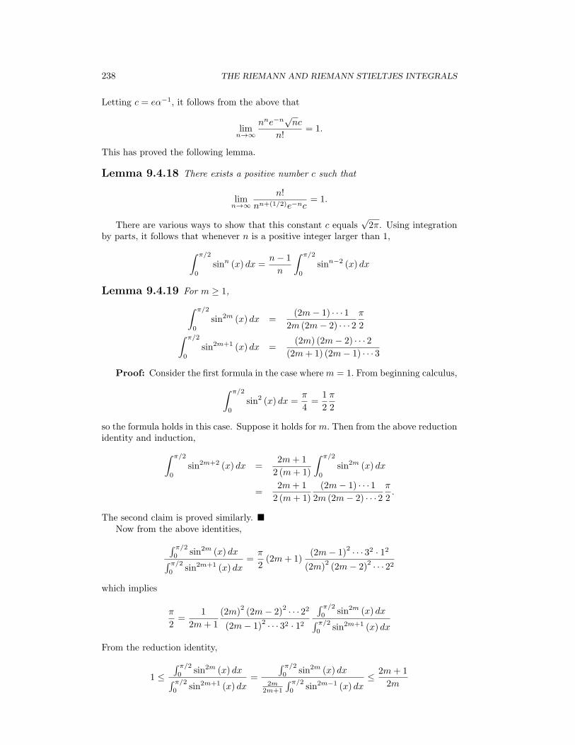
238 THE RIEMANN AND RIEMANN STIELTJES INTEGRALS
Letting c = eα−1, it follows from the above that
limn→∞
nne−n√nc
n!= 1.
This has proved the following lemma.
Lemma 9.4.18 There exists a positive number c such that
limn→∞
n!
nn+(1/2)e−nc= 1.
There are various ways to show that this constant c equals√2π. Using integration
by parts, it follows that whenever n is a positive integer larger than 1,∫ π/2
0
sinn (x) dx =n− 1
n
∫ π/2
0
sinn−2 (x) dx
Lemma 9.4.19 For m ≥ 1,∫ π/2
0
sin2m (x) dx =(2m− 1) · · · 1
2m (2m− 2) · · · 2π
2∫ π/2
0
sin2m+1 (x) dx =(2m) (2m− 2) · · · 2
(2m+ 1) (2m− 1) · · · 3
Proof: Consider the first formula in the case wherem = 1. From beginning calculus,∫ π/2
0
sin2 (x) dx =π
4=
1
2
π
2
so the formula holds in this case. Suppose it holds form. Then from the above reductionidentity and induction,∫ π/2
0
sin2m+2 (x) dx =2m+ 1
2 (m+ 1)
∫ π/2
0
sin2m (x) dx
=2m+ 1
2 (m+ 1)
(2m− 1) · · · 12m (2m− 2) · · · 2
π
2.
The second claim is proved similarly. �Now from the above identities,∫ π/2
0sin2m (x) dx∫ π/2
0sin2m+1 (x) dx
=π
2(2m+ 1)
(2m− 1)2 · · · 32 · 12
(2m)2(2m− 2)
2 · · · 22
which implies
π
2=
1
2m+ 1
(2m)2(2m− 2)
2 · · · 22
(2m− 1)2 · · · 32 · 12
∫ π/2
0sin2m (x) dx∫ π/2
0sin2m+1 (x) dx
From the reduction identity,
1 ≤∫ π/2
0sin2m (x) dx∫ π/2
0sin2m+1 (x) dx
=
∫ π/2
0sin2m (x) dx
2m2m+1
∫ π/2
0sin2m−1 (x) dx
≤ 2m+ 1
2m

9.4. THE RIEMANN STIELTJES INTEGRAL 239
It follows
2m
2m+ 12m
(2m− 2)2 · · · 22
(2m− 1)2 · · · 32 · 12
≤ π
2≤ 1
2m+ 1
(2m)2(2m− 2)
2 · · · 22
(2m− 1)2 · · · 32 · 12
2m+ 1
2m
= 2m(2m− 2)
2 · · · 22
(2m− 1)2 · · · 32 · 12
It follows that2m
2m+ 1≤ π/2
2m (2m−2)2···22(2m−1)2···32·12
≤ 1
and so
limm→∞
2m(2m− 2)
2 · · · 22
(2m− 1)2 · · · 32 · 12
=π
2
This is sometimes called Wallis’s formula. This implies
limm→∞
2m22m−2 ((m− 1)!)
2
(2m− 1)2 · · · 32 · 12
=π
2
Now multiply on the bottom and top by (2m)2(2m− 2)
2 · · · 22 = 22m (m!)2to obtain
limm→∞
2m22m−2 ((m− 1)!)
222m (m!)
2
((2m)!)2 = lim
m→∞22m2 2
2m−2 ((m− 1)!)222m (m!)
2
2m ((2m)!)2
limm→∞
22m (m!)222m (m!)
2
2m ((2m)!)2 =
π
2
It follows that
limm→∞
22m (m!)2
(2m)1/2
(2m)!=
√π
2(9.22)
Now with this result, it is possible to find c in Stirling’s formula. Recall
limm→∞
m!
mm+(1/2)e−mc= 1
It follows that
limm→∞
(2m)!
(2m)2m+(1/2)
e−2mc= 1
Therefore, from 9.22,√π
2= lim
m→∞
22m(
m!mm+(1/2)e−mc
)2 (mm+(1/2)e−mc
)2(2m)
1/2(
(2m)!
(2m)2m+(1/2)e−2mc
)((2m)
2m+(1/2)e−2mc
)= lim
m→∞
22m(mm+(1/2)e−mc
)2(2m)
1/2((2m)
2m+(1/2)e−2mc
)= lim
m→∞
22mm2m+1e−2mc2
(2m)1/2((2m)
2m+(1/2)e−2mc
)= lim
m→∞
22mm2m+1c
(2m)1/2
(2m)2m+(1/2)
=1
2c
which shows that c =√2π. This proves Stirling’s formula.

240 THE RIEMANN AND RIEMANN STIELTJES INTEGRALS
Theorem 9.4.20 The following formula holds.
limm→∞
(2m)!
(2m)2m+(1/2)
e−2m√2π
= 1
9.5 Exercises
1. Let F (x) =∫ x3
x2t5+7
t7+87t6+1 dt. Find F′ (x) .
2. Let F (x) =∫ x
21
1+t4 dt. Sketch a graph of F and explain why it looks the way itdoes.
3. Let a and b be positive numbers and consider the function
F (x) =
∫ ax
0
1
a2 + t2dt+
∫ a/x
b
1
a2 + t2dt.
Show that F is a constant.
4. Solve the following initial value problem from ordinary differential equations whichis to find a function y such that
y′ (x) =x7 + 1
x6 + 97x5 + 7, y (10) = 5.
5. If F,G ∈∫f (x) dx for all x ∈ R, show F (x) = G (x) + C for some constant, C.
Use this to give a different proof of the fundamental theorem of calculus which
has for its conclusion∫ b
af (t) dt = G (b)−G (a) where G′ (x) = f (x) .
6. Suppose f is continuous on [a, b]. Show there exists c ∈ (a, b) such that
f (c) =1
b− a
∫ b
a
f (x) dx.
Hint: You might consider the function F (x) ≡∫ x
af (t) dt and use the mean value
theorem for derivatives and the fundamental theorem of calculus.
7. Suppose f and g are continuous functions on [a, b] and that g (x) = 0 on (a, b) .Show there exists c ∈ (a, b) such that
f (c)
∫ b
a
g (x) dx =
∫ b
a
f (x) g (x) dx.
Hint: Define F (x) ≡∫ x
af (t) g (t) dt and let G (x) ≡
∫ x
ag (t) dt. Then use the
Cauchy mean value theorem on these two functions.
8. Consider the function
f (x) ≡{
sin(1x
)if x = 0
0 if x = 0.
Is f Riemann integrable? Explain why or why not.
9. Prove the second part of Theorem 9.2.2 about decreasing functions.

9.5. EXERCISES 241
10. The Riemann integral is only defined for bounded functions on bounded intervals.When f is Riemann integrable on [a,R] for each R > a define an “improper”integral as follows. ∫ ∞
a
f (t) dt ≡ limR→∞
∫ R
a
f (t) dt
whenever this limit exists. Show ∫ ∞
0
sinx
xdx
exists. Here the integrand is defined to equal 1 when x = 0, not that this matters.
11. Show ∫ ∞
0
sin(t2)dt
exists.
12. The Gamma function is defined for x > 0 by
Γ (x) ≡∫ ∞
0
e−ttx−1dt
Give a meaning to the above improper integral and show it exists. Also show
Γ (x+ 1) = Γ (x)x, Γ (1) = 1,
and for n a positive integer, Γ (n+ 1) = n!. Hint: The hard part is showing theintegral exists. To do this, first show that if f (x) is an increasing function whichis bounded above, then limx→∞ f (x) must exist and equal sup {f (x) : x ≥ 0} .Then show ∫ R
0
e−ttx−1dt ≡ limε→0+
∫ R
ε
e−ttx−1dt
is an increasing function of R which is bounded above.
13. The most important of all differential equations is the first order linear equation,y′+p (t) y = f (t) where p, f are continuous. Show the solution to the initial valueproblem consisting of this equation and the initial condition, y (a) = ya is
y (t) = e−P (t)ya + e−P (t)
∫ t
a
eP (s)f (s) ds,
where P (t) =∫ t
ap (s) ds. Give conditions under which everything is correct.
Hint: You use the integrating factor approach. Multiply both sides by eP (t),verify the left side equals
d
dt
(eP (t)y (t)
),
and then take the integral,∫ t
aof both sides.
14. Suppose f is a continuous function which is not equal to zero on [0, b] . Show that∫ b
0
f (x)
f (x) + f (b− x)dx =
b
2.
Hint: First change the variables to obtain the integral equals∫ b/2
−b/2
f (y + b/2)
f (y + b/2) + f (b/2− y)dy

242 THE RIEMANN AND RIEMANN STIELTJES INTEGRALS
Next show by another change of variables that this integral equals∫ b/2
−b/2
f (b/2− y)f (y + b/2) + f (b/2− y)
dy.
Thus the sum of these equals b.
15. Let there be three equally spaced points, xi−1, xi−1 + h ≡ xi, and xi +2h ≡ xi+1.Suppose also a function f, has the value fi−1 at x, fi at x+h, and fi+1 at x+2h.Then consider
gi (x) ≡fi−1
2h2(x− xi) (x− xi+1)−
fih2
(x− xi−1) (x− xi+1)+fi+1
2h2(x− xi−1) (x− xi) .
Check that this is a second degree polynomial which equals the values fi−1, fi,and fi+1 at the points xi−1, xi, and xi+1 respectively. The function gi is anapproximation to the function f on the interval [xi−1, xi+1] . Also,∫ xi+1
xi−1
gi (x) dx
is an approximation to∫ xi+1
xi−1f (x) dx. Show
∫ xi+1
xi−1gi (x) dx equals
hfi−1
3+hfi4
3+hfi+1
3.
Now suppose n is even and {x0, x1, · · · , xn} is a partition of the interval, [a, b] andthe values of a function f defined on this interval are fi = f (xi) . Adding theseapproximations for the integral of f on the succession of intervals,
[x0, x2] , [x2, x4] , · · · , [xn−2, xn] ,
show that an approximation to∫ b
af (x) dx is
h
3[f0 + 4f1 + 2f2 + 4f3 + 2f2 + · · ·+ 4fn−1 + fn] .
This is called Simpson’s rule. Use Simpson’s rule to compute an approximation
to∫ 2
11t dt letting n = 4.
16. Suppose x0 ∈ (a, b) and that f is a function which has n+1 continuous derivativeson this interval. Consider the following.
f (x) = f (x0) +
∫ x
x0
f ′ (t) dt
= f (x0) + (t− x) f ′ (t) |xx0+
∫ x
x0
(x− t) f ′′ (t) dt
= f (x0) + f ′ (x0) (x− x0) +∫ x
x0
(x− t) f ′′ (t) dt.
Explain the above steps and continue the process to eventually obtain Taylor’sformula,
f (x) = f (x0) +n∑
k=1
f (k) (x0)
k!(x− x0)k +
1
n!
∫ x
x0
(x− t)n f (n+1) (t) dt
where n! ≡ n (n− 1) · · · 3 · 2 · 1 if n ≥ 1 and 0! ≡ 1.

9.5. EXERCISES 243
17. In the above Taylor’s formula, use Problem 7 on Page 240 to obtain the existenceof some z between x0 and x such that
f (x) = f (x0) +n∑
k=1
f (k) (x0)
k!(x− x0)k +
f (n+1) (z)
(n+ 1)!(x− x0)n+1
.
Hint: You might consider two cases, the case when x > x0 and the case whenx < x0.
18. There is a general procedure for constructing methods of approximate integrationlike the trapezoid rule and Simpson’s rule. Consider [0, 1] and divide this intervalinto n pieces using a uniform partition, {x0, · · · , xn} where xi − xi−1 = 1/n foreach i. The approximate integration scheme for a function f, will be of the form(
1
n
) n∑i=0
cifi ≈∫ 1
0
f (x) dx
where fi = f (xi) and the constants, ci are chosen in such a way that the above
sum gives the exact answer for∫ 1
0f (x) dx where f (x) = 1, x, x2, · · · , xn. When
this has been done, change variables to write∫ b
a
f (y) dy = (b− a)∫ 1
0
f (a+ (b− a)x) dx
≈ b− an
n∑i=1
cif
(a+ (b− a)
(i
n
))
=b− an
n∑i=1
cifi
where fi = f(a+ (b− a)
(in
)). Consider the case where n = 1. It is necessary to
find constants c0 and c1 such that
c0 + c1 = 1 =∫ 1
01 dx
0c0 + c1 = 1/2 =∫ 1
0x dx.
Show that c0 = c1 = 1/2, and that this yields the trapezoid rule. Next taken = 2 and show the above procedure yields Simpson’s rule. Show also that ifthis integration scheme is applied to any polynomial of degree 3 the result will beexact. That is,
1
2
(1
3f0 +
4
3f1 +
1
3f2
)=
∫ 1
0
f (x) dx
whenever f (x) is a polynomial of degree three. Show that if fi are the values of f at
a, a+b2 , and b with f1 = f
(a+b2
), it follows that the above formula gives
∫ b
af (x) dx
exactly whenever f is a polynomial of degree three. Obtain an integration schemefor n = 3.
19. Let f have four continuous derivatives on [xi−1, xi+1] where xi+1 = xi−1+2h andxi = xi−1 + h. Show using Problem 17, there exists a polynomial of degree three,p3 (x) , such that
f (x) = p3 (x) +1
4!f (4) (ξ) (x− xi)4
Now use Problem 18 and Problem 15 to conclude∣∣∣∣∣∫ xi+1
xi−1
f (x) dx−(hfi−1
3+hfi4
3+hfi+1
3
)∣∣∣∣∣ < M
4!
2h5
5,

244 THE RIEMANN AND RIEMANN STIELTJES INTEGRALS
where M satisfies, M ≥ max{∣∣f (4) (t)∣∣ : t ∈ [xi−1, xi]
}. Now let S (a, b, f, 2m)
denote the approximation to∫ b
af (x) dx obtained from Simpson’s rule using 2m
equally spaced points. Show∣∣∣∣∣∫ b
a
f (x) dx− S (a, b, f, 2m)
∣∣∣∣∣ < M
1920(b− a)5 1
m4
whereM ≥ max{∣∣f (4) (t)∣∣ : t ∈ [a, b]
}. Better estimates are available in numerical
analysis books. However, these also have the error in the form C(1/m4
).
20. A regular Sturm Liouville problem involves the differential equation, for anunknown function of x which is denoted here by y,
(p (x) y′)′+ (λq (x) + r (x)) y = 0, x ∈ [a, b]
and it is assumed that p (t) , q (t) > 0 for any t along with boundary conditions,
C1y (a) + C2y′ (a) = 0
C3y (b) + C4y′ (b) = 0
whereC2
1 + C22 > 0, and C2
3 + C24 > 0.
There is an imense theory connected to these important problems. The constant,λ is called an eigenvalue. Show that if y is a solution to the above problemcorresponding toλ = λ1 and if z is a solution corresponding to λ = λ2 = λ1, then∫ b
a
q (x) y (x) z (x) dx = 0. (9.23)
Hint: Do something like this:
(p (x) y′)′z + (λ1q (x) + r (x)) yz = 0,
(p (x) z′)′y + (λ2q (x) + r (x)) zy = 0.
Now subtract and either use integration by parts or show
(p (x) y′)′z − (p (x) z′)
′y = ((p (x) y′) z − (p (x) z′) y)
′
and then integrate. Use the boundary conditions to show that y′ (a) z (a) −z′ (a) y (a) = 0 and y′ (b) z (b) − z′ (b) y (b) = 0. The formula, 9.23 is called anorthogonality relation and it makes possible an expansion in terms of certainfunctions called eigenfunctions.
21. Letting [a, b] = [−π, π] , consider an example of a regular Sturm Liouville problemwhich is of the form
y′′ + λy = 0, y (−π) = 0, y (π) = 0.
Show that if λ = n2 and yn (x) = sin (nx) for n a positive integer, then yn is asolution to this regular Sturm Liouville problem. In this case, q (x) = 1 and sofrom Problem 20, it must be the case that∫ π
−π
sin (nx) sin (mx) dx = 0
if n = m. Show directly using integration by parts that the above equation is true.
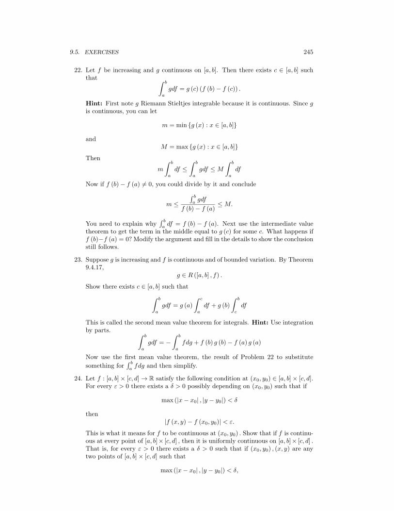
9.5. EXERCISES 245
22. Let f be increasing and g continuous on [a, b]. Then there exists c ∈ [a, b] suchthat ∫ b
a
gdf = g (c) (f (b)− f (c)) .
Hint: First note g Riemann Stieltjes integrable because it is continuous. Since gis continuous, you can let
m = min {g (x) : x ∈ [a, b]}
andM = max {g (x) : x ∈ [a, b]}
Then
m
∫ b
a
df ≤∫ b
a
gdf ≤M∫ b
a
df
Now if f (b)− f (a) = 0, you could divide by it and conclude
m ≤∫ b
agdf
f (b)− f (a)≤M.
You need to explain why∫ b
adf = f (b) − f (a). Next use the intermediate value
theorem to get the term in the middle equal to g (c) for some c. What happens iff (b)−f (a) = 0? Modify the argument and fill in the details to show the conclusionstill follows.
23. Suppose g is increasing and f is continuous and of bounded variation. By Theorem9.4.17,
g ∈ R ([a, b] , f) .
Show there exists c ∈ [a, b] such that∫ b
a
gdf = g (a)
∫ c
a
df + g (b)
∫ b
c
df
This is called the second mean value theorem for integrals. Hint: Use integrationby parts. ∫ b
a
gdf = −∫ b
a
fdg + f (b) g (b)− f (a) g (a)
Now use the first mean value theorem, the result of Problem 22 to substitute
something for∫ b
afdg and then simplify.
24. Let f : [a, b]× [c, d]→ R satisfy the following condition at (x0, y0) ∈ [a, b]× [c, d].For every ε > 0 there exists a δ > 0 possibly depending on (x0, y0) such that if
max (|x− x0| , |y − y0|) < δ
then|f (x, y)− f (x0, y0)| < ε.
This is what it means for f to be continuous at (x0, y0) . Show that if f is continu-ous at every point of [a, b]× [c, d] , then it is uniformly continuous on [a, b]× [c, d] .That is, for every ε > 0 there exists a δ > 0 such that if (x0, y0) , (x, y) are anytwo points of [a, b]× [c, d] such that
max (|x− x0| , |y − y0|) < δ,

246 THE RIEMANN AND RIEMANN STIELTJES INTEGRALS
then
|f (x, y)− f (x0, y0)| < ε.
Also show that such a function achieves its maximum and its minimum on [a, b]×[c, d] . Hint: This is easy if you follow the same procedure that was used earlierbut you take subsequences for each component to show [a, b]× [c, d] is sequentiallycompact.
25. Suppose f is a real valued function defined on [a, b]× [c, d] which is uniformly con-tinuous as described in Problem 24 and bounded which follow from an assumptionthat it is continuous. Also suppose α, β are increasing functions. Show
x→∫ d
c
f (x, y) dβ (y) , y →∫ b
a
f (x, y) dα (x)
are both continuous functions. The idea is you fix one of the variables, x in thefirst and then integrate the continuous function of y obtaining a real number whichdepends on the value of x fixed. Explain why it makes sense to write∫ b
a
∫ d
c
f (x, y) dβ (y) dα (x) ,
∫ d
c
∫ b
a
f (x, y) dα (x) dβ (y) .
Now consider the first of the above iterated integrals. (That is what these arecalled.) Consider the following argument in which you fill in the details.∫ b
a
∫ d
c
f (x, y) dβ (y) dα (x) =n∑
i=1
∫ xi
xi−1
∫ d
c
f (x, y) dβ (y) dα (x)
=n∑
i=1
∫ xi
xi−1
m∑j=1
∫ yj
yj−1
f (x, y) dβ (y) dα (x)
=
n∑i=1
m∑j=1
∫ xi
xi−1
∫ yj
yj−1
f (x, y) dβ (y) dα (x)
=n∑
i=1
m∑j=1
∫ xi
xi−1
(β (yj)− β (yj−1)) f (x, tj) dα (x)
=n∑
i=1
m∑j=1
(β (yj)− β (yj−1)) (α (xi)− α (xj−1)) f (sj , tj)
Also ∫ d
c
∫ b
a
f (x, y) dα (x) dβ (y)
=m∑j=1
n∑i=1
(β (yj)− β (yj−1)) (α (xi)− α (xj−1)) f(s′j , t
′j
)and now because of uniform continuity, it follows that if the partition points areclose enough, ∣∣f (s′j , t′j)− f (sj , tj)∣∣ < ε
(β (d)− β (c)) (α (b)− α (a))

9.5. EXERCISES 247
and so ∣∣∣∣∣∫ d
c
∫ b
a
f (x, y) dα (x) dβ (y)−∫ d
c
∫ b
a
f (x, y) dα (x) dβ (y)
∣∣∣∣∣ < ε
Since ε is arbitrary, this shows the two iterated integrals are equal. This is a caseof Fubini’s theorem.
26. Generalize the result of Problem 25 to the situation where α and β are only ofbounded variation.
27. This problem is in Apostol [2]. Explain why whenever f is continuous on [a, b]
limn→∞
b− an
n∑k=1
f
(a+ k
(b− an
))=
∫ b
a
fdx.
Apply this to f (x) = 11+x2 on the interval [0, 1] to obtain the very interesting
formulaπ
4= lim
n→∞
n∑k=1
n
n2 + k2.
28. Suppose f : [a, b] × (c, d) → R is continuous. Recall the meaning of the partialderivative from calculus,
∂f
∂x(t, x) ≡ lim
h→0
f (t, x+ h)− f (t, x)h
Suppose also∂f
∂x(t, x)
exists and for some K independent of t,∣∣∣∣∂f∂x (t, z)− ∂f
∂x(t, x)
∣∣∣∣ < K |z − x| .
This last condition happens, for example if ∂2f(t,x)∂x2 is uniformly bounded on [a, b]×
(c, d) . (Why?) Define
F (x) ≡∫ b
a
f (t, x) dt.
Take the difference quotient of F and show using the mean value theorem and theabove assumptions that
F ′ (x) =
∫ b
a
∂f (t, x)
∂xdt.
Is there a version of this result with dt replaced with dα where α is an increasingfunction? How about α a function of bounded variation?
29. I found this problem in Apostol’s book [2]. This is a very important result and isobtained very simply. Let
g (x) ≡∫ 1
0
e−x2(1+t2)
1 + t2dt
and
f (x) ≡(∫ x
0
e−t2dt
)2
.
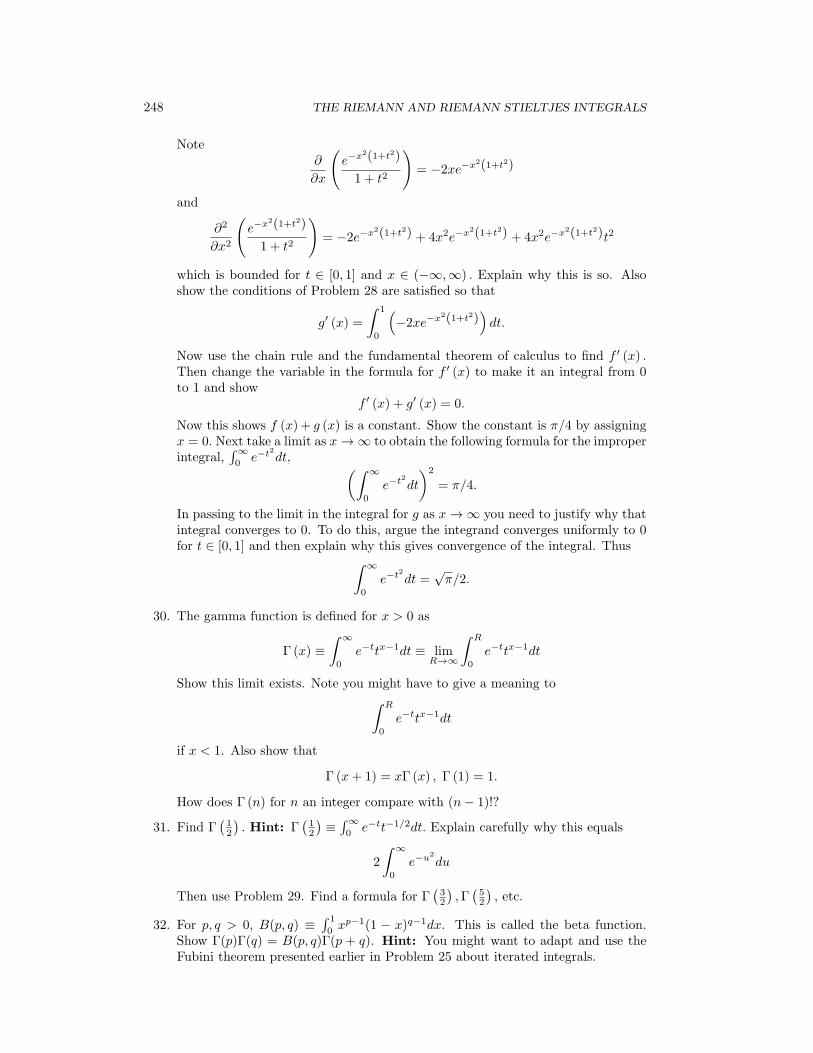
248 THE RIEMANN AND RIEMANN STIELTJES INTEGRALS
Note∂
∂x
(e−x2(1+t2)
1 + t2
)= −2xe−x2(1+t2)
and
∂2
∂x2
(e−x2(1+t2)
1 + t2
)= −2e−x2(1+t2) + 4x2e−x2(1+t2) + 4x2e−x2(1+t2)t2
which is bounded for t ∈ [0, 1] and x ∈ (−∞,∞) . Explain why this is so. Alsoshow the conditions of Problem 28 are satisfied so that
g′ (x) =
∫ 1
0
(−2xe−x2(1+t2)
)dt.
Now use the chain rule and the fundamental theorem of calculus to find f ′ (x) .Then change the variable in the formula for f ′ (x) to make it an integral from 0to 1 and show
f ′ (x) + g′ (x) = 0.
Now this shows f (x) + g (x) is a constant. Show the constant is π/4 by assigningx = 0. Next take a limit as x→∞ to obtain the following formula for the improperintegral,
∫∞0e−t2dt, (∫ ∞
0
e−t2dt
)2
= π/4.
In passing to the limit in the integral for g as x→∞ you need to justify why thatintegral converges to 0. To do this, argue the integrand converges uniformly to 0for t ∈ [0, 1] and then explain why this gives convergence of the integral. Thus∫ ∞
0
e−t2dt =√π/2.
30. The gamma function is defined for x > 0 as
Γ (x) ≡∫ ∞
0
e−ttx−1dt ≡ limR→∞
∫ R
0
e−ttx−1dt
Show this limit exists. Note you might have to give a meaning to∫ R
0
e−ttx−1dt
if x < 1. Also show that
Γ (x+ 1) = xΓ (x) , Γ (1) = 1.
How does Γ (n) for n an integer compare with (n− 1)!?
31. Find Γ(12
). Hint: Γ
(12
)≡∫∞0e−tt−1/2dt. Explain carefully why this equals
2
∫ ∞
0
e−u2
du
Then use Problem 29. Find a formula for Γ(32
),Γ(52
), etc.
32. For p, q > 0, B(p, q) ≡∫ 1
0xp−1(1 − x)q−1dx. This is called the beta function.
Show Γ(p)Γ(q) = B(p, q)Γ(p + q). Hint: You might want to adapt and use theFubini theorem presented earlier in Problem 25 about iterated integrals.

Fourier Series
10.1 The Complex Exponential
What does eix mean? Here i2 = −1. Recall the complex numbers are of the form a+ iband are identified as points in the plane. For f (x) = eix, you would want
f ′′ (x) = i2f (x) = −f (x)
sof ′′ (x) + f (x) = 0.
Also, you would wantf (0) = e0 = 1, f ′ (0) = ie0 = i.
One solution to these conditions is
f (x) = cos (x) + i sin (x) .
Is it the only solution? Suppose g (x) is another solution. Consider u (x) = f (x)−g (x) .Then it follows
u′′ (x) + u (x) = 0, u (0) = 0 = u′ (0) .
Thus both Reu and Imu solve the differential equation and 0 initial condition. ByLemma 8.3.3 both Reu and Imu are equal to 0. Thus the above is the only solution.Recall by De’Moivre’s theorem
(cosx+ i sinx)n= cos (nx) + i sin (nx)
for any integer n and so (eix)n
= einx.
10.2 Definition And Basic Properties
A Fourier series is an expression of the form
∞∑k=−∞
ckeikx
where this means
limn→∞
n∑k=−n
ckeikx.
Obviously such a sequence of partial sums may or may not converge at a particularvalue of x.
249

250 FOURIER SERIES
These series have been important in applied math since the time of Fourier whowas an officer in Napoleon’s army. He was interested in studying the flow of heat incannons and invented the concept to aid him in his study. Since that time, Fourierseries and the mathematical problems related to their convergence have motivated thedevelopment of modern methods in analysis. As recently as the mid 1960’s a problemrelated to convergence of Fourier series was solved for the first time and the solution ofthis problem was a big surprise.1 This chapter is on the classical theory of convergenceof Fourier series.
If you can approximate a function f with an expression of the form
∞∑k=−∞
ckeikx
then the function must have the property f (x+ 2π) = f (x) because this is true ofevery term in the above series. More generally, here is a definition.
Definition 10.2.1 A function f defined on R is a periodic function of periodT if f (x+ T ) = f (x) for all x.
As just explained, Fourier series are useful for representing periodic functions andno other kind of function.There is no loss of generality in studying only functions whichare periodic of period 2π. Indeed, if f is a function which has period T , you can studythis function in terms of the function g (x) ≡ f
(Tx2π
)where g is periodic of period 2π.
Definition 10.2.2 For f ∈ R ([−π, π]) and f periodic on R, define the Fourierseries of f as
∞∑k=−∞
ckeikx, (10.1)
where
ck ≡1
2π
∫ π
−π
f (y) e−ikydy. (10.2)
Also define the nth partial sum of the Fourier series of f by
Sn (f) (x) ≡n∑
k=−n
ckeikx. (10.3)
It may be interesting to see where this formula came from. Suppose then that
f (x) =∞∑
k=−∞
ckeikx,
multiply both sides by e−imx and take the integral∫ π
−π, so that
∫ π
−π
f (x) e−imxdx =
∫ π
−π
∞∑k=−∞
ckeikxe−imxdx.
1The question was whether the Fourier series of a function in L2 converged a.e. to the function.It turned out that it did, to the surprise of many because it was known that the Fourier series of afunction in L1 does not necessarily converge to the function a.e. The problem was solved by Carlesonin 1965.
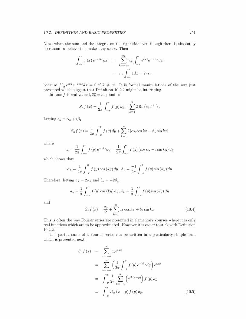
10.2. DEFINITION AND BASIC PROPERTIES 251
Now switch the sum and the integral on the right side even though there is absolutelyno reason to believe this makes any sense. Then∫ π
−π
f (x) e−imxdx =∞∑
k=−∞
ck
∫ π
−π
eikxe−imxdx
= cm
∫ π
−π
1dx = 2πcm
because∫ π
−πeikxe−imxdx = 0 if k = m. It is formal manipulations of the sort just
presented which suggest that Definition 10.2.2 might be interesting.In case f is real valued, ck = c−k and so
Snf (x) =1
2π
∫ π
−π
f (y) dy +
n∑k=1
2Re(cke
ikx).
Letting ck ≡ αk + iβk
Snf (x) =1
2π
∫ π
−π
f (y) dy +n∑
k=1
2 [αk cos kx− βk sin kx]
where
ck =1
2π
∫ π
−π
f (y) e−ikydy =1
2π
∫ π
−π
f (y) (cos ky − i sin ky) dy
which shows that
αk =1
2π
∫ π
−π
f (y) cos (ky) dy, βk =−12π
∫ π
−π
f (y) sin (ky) dy
Therefore, letting ak = 2αk and bk = −2βk,
ak =1
π
∫ π
−π
f (y) cos (ky) dy, bk =1
π
∫ π
−π
f (y) sin (ky) dy
and
Snf (x) =a02
+n∑
k=1
ak cos kx+ bk sin kx (10.4)
This is often the way Fourier series are presented in elementary courses where it is onlyreal functions which are to be approximated. However it is easier to stick with Definition10.2.2.
The partial sums of a Fourier series can be written in a particularly simple formwhich is presented next.
Snf (x) =n∑
k=−n
ckeikx
=
n∑k=−n
(1
2π
∫ π
−π
f (y) e−ikydy
)eikx
=
∫ π
−π
1
2π
n∑k=−n
(eik(x−y)
)f (y) dy
≡∫ π
−π
Dn (x− y) f (y) dy. (10.5)

252 FOURIER SERIES
The function
Dn (t) ≡1
2π
n∑k=−n
eikt
is called the Dirichlet Kernel
Theorem 10.2.3 The function Dn satisfies the following:
1.∫ π
−πDn (t) dt = 1
2. Dn is periodic of period 2π
3. Dn (t) = (2π)−1 sin(n+ 1
2 )tsin( t
2 ).
Proof:Part 1 is obvious because 12π
∫ π
−πe−ikydy = 0 whenever k = 0 and it equals 1
if k = 0. Part 2 is also obvious because t→ eikt is periodic of period 2π. It remains toverify Part 3. Note
2πDn (t) =
n∑k=−n
eikt = 1 + 2
n∑k=1
cos (kt)
Therefore,
2πDn (t) sin
(t
2
)= sin
(t
2
)+ 2
n∑k=1
sin
(t
2
)cos (kt)
= sin
(t
2
)+
n∑k=1
sin
((k +
1
2
)t
)− sin
((k − 1
2
)t
)= sin
((n+
1
2
)t
)where the easily verified trig. identity cos (a) sin (b) = 1
2 (sin (a+ b)− sin (a− b)) is usedto get to the second line. This proves 3 and proves the theorem.
Here is a picture of the Dirichlet kernels for n=1,2, and 3
x
0−1−2 1
1
−1
0
32
2
−3
y
Note they are not nonnegative but there is a large central positive bump which getslarger as n gets larger.
It is not reasonable to expect a Fourier series to converge to the function at everypoint. To see this, change the value of the function at a single point in (−π, π) andextend to keep the modified function periodic. Then the Fourier series of the modifiedfunction is the same as the Fourier series of the original function and so if pointwiseconvergence did take place, it no longer does. However, it is possible to prove aninteresting theorem about pointwise convergence of Fourier series. This is done next.

10.3. THE RIEMANN LEBESGUE LEMMA 253
10.3 The Riemann Lebesgue Lemma
The Riemann Lebesgue lemma is the basic result which makes possible the study ofpointwise convergence of Fourier series. It is also a major result in other contexts andserves as a useful example.
For the purpose of simple notation, let R ((a, b]) denote those functions f which arein R ([a+ δ, b]) for every δ > 0 and the improper integral
limδ→0
∫ b
a+δ
f (x) dx exists.
Lemma 10.3.1 Let f ∈ R ((a, b]) , f (x) ≥ 0, where (a, b) is some finite intervaland let ε > 0. Then there exists an interval of finite length, [a1, b1] ⊆ (a, b) and adifferentiable function h having continuous derivative such that both h and h′ equal 0outside of [a1, b1] which has the property that 0 ≤ h (x) ≤ f (x) and∫ b
a
|f − h| dx < ε (10.6)
Proof: First here is a claim.Claim: There exists a continuous g which vanishes near a and b such that g ≤ f
and ∫ b
a
|f (x)− g (x)| dx < ε/3.
where the integral is the improper Riemann integral defined by∫ b
a
(f (x)− g (x)) dx ≡ limδ→0+
∫ b
a+δ
(f (x)− g (x)) dx
Proof of the claim: First let a0 > a such that∣∣∣∣∣∫ b
a
f (x) dx−∫ b
a0
f (x) dx
∣∣∣∣∣ =∫ a0
a
|f (x)| dx < ε/3.
Let {x0, x1, · · · , xn} be a partition of [a0, b] and let
n∑k=1
ak (xk − xk−1)
be a lower sum such that∣∣∣∣∣∫ b
a0
f (x) dx−n∑
k=1
ak (xk − xk−1)
∣∣∣∣∣ < ε/6.
The sum in the above equals ∫ b
a0
n∑k=1
akX[xk−1,xk) (x) dx
where
X[xk−1,xk) (x) =
{1 if x ∈ [xk−1, xk)0 if x /∈ [xk−1, xk)
Now let ψk be a continuous function which approximates X[xk−1,xk) (x) and vanishes nearthe endpoints of [xk−1, xk) as shown in the following picture in which δ is sufficientlysmall.
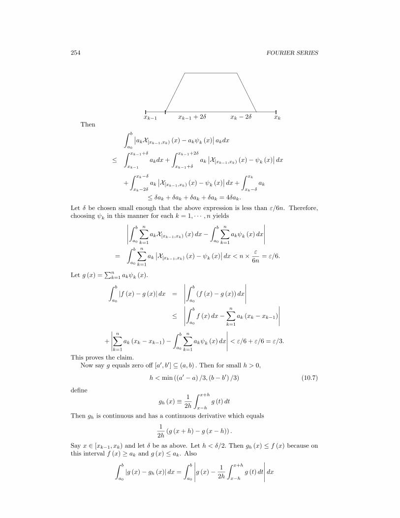
254 FOURIER SERIES
������ A
AAAAA
xk−1 xk−1 + 2δ xk − 2δ xkThen ∫ b
a0
∣∣akX[xk−1,xk) (x)− akψk (x)∣∣ akdx
≤∫ xk−1+δ
xk−1
akdx+
∫ xk−1+2δ
xk−1+δ
ak∣∣X[xk−1,xk) (x)− ψk (x)
∣∣ dx+
∫ xk−δ
xk−2δ
ak∣∣X[xk−1,xk) (x)− ψk (x)
∣∣ dx+
∫ xk
xk−δ
ak
≤ δak + δak + δak + δak = 4δak.
Let δ be chosen small enough that the above expression is less than ε/6n. Therefore,choosing ψk in this manner for each k = 1, · · · , n yields∣∣∣∣∣
∫ b
a0
n∑k=1
akX[xk−1,xk) (x) dx−∫ b
a0
n∑k=1
akψk (x) dx
∣∣∣∣∣=
∫ b
a0
n∑k=1
ak∣∣X[xk−1,xk) (x)− ψk (x)
∣∣ dx < n× ε
6n= ε/6.
Let g (x) =∑n
k=1 akψk (x).∫ b
a0
|f (x)− g (x)| dx =
∣∣∣∣∣∫ b
a0
(f (x)− g (x)) dx
∣∣∣∣∣≤
∣∣∣∣∣∫ b
a0
f (x) dx−n∑
k=1
ak (xk − xk−1)
∣∣∣∣∣+
∣∣∣∣∣n∑
k=1
ak (xk − xk−1)−∫ b
a0
n∑k=1
akψk (x) dx
∣∣∣∣∣ < ε/6 + ε/6 = ε/3.
This proves the claim.Now say g equals zero off [a′, b′] ⊆ (a, b) . Then for small h > 0,
h < min ((a′ − a) /3, (b− b′) /3) (10.7)
define
gh (x) ≡1
2h
∫ x+h
x−h
g (t) dt
Then gh is continuous and has a continuous derivative which equals
1
2h(g (x+ h)− g (x− h)) .
Say x ∈ [xk−1, xk) and let δ be as above. Let h < δ/2. Then gh (x) ≤ f (x) because onthis interval f (x) ≥ ak and g (x) ≤ ak. Also∫ b
a0
|g (x)− gh (x)| dx =
∫ b
a0
∣∣∣∣∣g (x)− 1
2h
∫ x+h
x−h
g (t) dt
∣∣∣∣∣ dx

10.3. THE RIEMANN LEBESGUE LEMMA 255
=
∫ b
a0
∣∣∣∣∣ 12h∫ x+h
x−h
(g (x)− g (t)) dt
∣∣∣∣∣ dx ≤∫ b
a0
1
2h
∫ x+h
x−h
|g (x)− g (t)| dtdx
<
∫ b
a0
1
2h
∫ x+h
x−h
ε
3 (b− a0)dtdx =
ε
3
provided h is small enough, due to the uniform continuity of g. (Why is g uniformlycontinuous?) Also, since h satisfies 10.7, gh and g′h vanish outside some closed interval,[a1, b1] ⊆ (a0, b). Since gh equals zero between a and a0, this shows that for such h,∫ b
a
|f (x)− gh (x)| dx =
∣∣∣∣∣∫ b
a
f (x) dx−∫ b
a
gh (x) dx
∣∣∣∣∣≤
∣∣∣∣∣∫ b
a
f (x) dx−∫ b
a0
f (x) dx
∣∣∣∣∣+∣∣∣∣∣∫ b
a0
f (x) dx−∫ b
a0
gh (x) dx
∣∣∣∣∣≤ ε
3+
∣∣∣∣∣∫ b
a0
f (x) dx−∫ b
a0
g (x) dx
∣∣∣∣∣+∣∣∣∣∣∫ b
a0
g (x) dx−∫ b
a0
gh (x) dx
∣∣∣∣∣< ε/3 + ε/3 + ε/3 = ε.
Letting h = gh this proves the Lemma.The lemma can be generalized to the case where f has values in C. In this case,∫ b
a
f (x) dx ≡∫ b
a
Re f (x) dx+ i
∫ b
a
Im f (x) dx
and f ∈ R ((a, b]) means Re f, Im f ∈ R ((a, b]).
Lemma 10.3.2 Let |f | ∈ R ((a, b]) , where (a, b) is some finite interval and let ε > 0.Then there exists an interval of finite length, [a1, b1] ⊆ (a, b) and a differentiable functionh having continuous derivative such that both h and h′ equal 0 outside of [a1, b1] whichhas the property that ∫ b
a
|f − h| dx < ε (10.8)
Proof: For g a real valued bounded function, define
g+ (x) ≡ g (x) + |g (x)|2
, g− (x) ≡ |g (x)| − g (x)2
.
First suppose f is real valued. Then apply Lemma 10.3.2 to f+ and f− to obtain h+and h− continuous and vanishing on some interval, [a1, b1] ⊆ (a, b) such that∫ b
a
(f+ − h+) dx < ε/5,
∫ b
a
(f− − h−) dx < ε/5
Let h = h+ − h−. Then if f (x) ≥ 0, f− (x) = 0 and so
f (x)− h (x) = f+ (x)− h+ (x) + h− (x) = f+ (x)− h+ (x) ≥ 0
If f (x) < 0, then f+ (x) = 0 and so h+ (x) = 0 and
h (x)− f (x) = −h− (x)− (−f− (x)) = f− (x)− h− (x) ≥ 0.
256 FOURIER SERIES
Therefore, |f (x)− h (x)| ≤ f+ (x)− h+ (x) + (f− (x)− h− (x)) and so∫ b
a
|f − h| dx ≤∫ b
a
(f+ − h+) dx+
∫ b
a
(f− − h−) dx <2ε
5.
Now if f has values in C, from what was just shown, there exist h1, h2 continuousand vanishing on some interval, [a1, b1] ⊆ (a, b) such that∫ b
a
|Re f − h1| dx,∫ b
a
|Im f − h2| dx <2ε
5
and therefore, ∫ b
a
|Re f + i Im f − (h1 + ih2)| dx ≤∫ b
a
|Re f − h1| dx
+
∫ b
a
|Im f − h2| dx <4ε
5< ε.
This proves the lemma.The lemma is the basis for the Riemann Lebesgue lemma, the main result in the
study of pointwise convergence of Fourier series.
Lemma 10.3.3 (Riemann Lebesgue) Let |f | ∈ R ((a, b]) where (a, b) is some finiteinterval. Then
limα→∞
∫ b
a
f (t) sin (αt+ β) dt = 0. (10.9)
Here the integral is the improper Riemann integral defined by
limδ→0+
∫ b
a+δ
f (t) sin (αt+ β) dt
Proof: Let ε > 0 be given and use Lemma 10.3.2 to obtain g such that g and g′ areboth continuous and vanish outside [a1, b1] ⊆ (a, b), and∫ b
a
|g − f | dx < ε
2. (10.10)
Then ∣∣∣∣∣∫ b
a
f (t) sin (αt+ β) dt
∣∣∣∣∣ ≤∣∣∣∣∣∫ b
a
(f (t)− g (t)) sin (αt+ β) dt
∣∣∣∣∣+
∣∣∣∣∣∫ b
a
g (t) sin (αt+ β) dt
∣∣∣∣∣≤
∫ b
a
|f − g| dx+
∣∣∣∣∣∫ b
a
g (t) sin (αt+ β) dt
∣∣∣∣∣<
ε
2+
∣∣∣∣∣∫ b1
a1
g (t) sin (αt+ β) dt
∣∣∣∣∣ .
10.4. DINI’S CRITERION FOR CONVERGENCE 257
Integrate the last term by parts.∫ b1
a1
g (t) sin (αt+ β) dt =− cos (αt+ β)
αg (t) |b1a1
+
∫ b1
a1
cos (αt+ β)
αg′ (t) dt,
an expression which converges to zero since g′ is bounded and
− cos (αt+ β)
αg (t) |b1a1
= 0
because g vanishes at a1 and b1. Therefore, taking α large enough,∣∣∣∣∣∫ b
a
f (t) sin (αt+ β) dt
∣∣∣∣∣ < ε
2+ε
2= ε
and this proves the lemma.
10.4 Dini’s Criterion For Convergence
Fourier series like to converge to the midpoint of the jump of a function under certainconditions. The condition given for convergence in the following theorem is due to Dini.It is a generalization of the usual theorem presented in elementary books on Fourierseries methods. [3].
Recalllim
t→x+f (t) ≡ f (x+) , and lim
t→x−f (t) ≡ f (x−)
Theorem 10.4.1 Let f be a periodic function of period 2π which is in R ([−π, π]).Suppose at some x, f (x+) and f (x−) both exist and that the function
y →∣∣∣∣f (x− y)− f (x−) + f (x+ y)− f (x+)
y
∣∣∣∣ ≡ h (y) (10.11)
is in R ((0, π]) which means
limε→0+
∫ π
ε
h (y) dy exists (10.12)
Then
limn→∞
Snf (x) =f (x+) + f (x−)
2. (10.13)
Proof:
Snf (x) =
∫ π
−π
Dn (x− y) f (y) dy
Change variables x− y → y and use the periodicity of f and Dn along with the formulafor Dn (y) to write this as
Snf (x) =
∫ π
−π
Dn (y) f (x− y)
=
∫ π
0
Dn (y) f (x− y) dy +∫ 0
−π
Dn (y) f (x− y) dy
=
∫ π
0
Dn (y) [f (x− y) + f (x+ y)] dy
=
∫ π
0
1
π
sin((n+ 1
2
)y)
sin(y2
) [f (x− y) + f (x+ y)
2
]dy. (10.14)
258 FOURIER SERIES
Note the function
y → 1
π
sin((n+ 1
2
)y)
sin(y2
) ,
while it is not defined at 0, is at least bounded and by L’Hospital’s rule,
limy→0
1
π
sin((n+ 1
2
)y)
sin(y2
) =2n+ 1
π
so defining it to equal this value at 0 yields a continuous, hence Riemann integrablefunction and so the above integral at least makes sense. Also from the property that∫ π
−πDn (t) dt = 1,
f (x+) + f (x−) =
∫ π
−π
Dn (y) [f (x+) + f (x−)] dy
= 2
∫ π
0
Dn (y) [f (x+) + f (x−)] dy
=
∫ π
0
1
π
sin((n+ 1
2
)y)
sin(y2
) [f (x+) + f (x−)] dy
and so ∣∣∣∣Snf (x)−f (x+) + f (x−)
2
∣∣∣∣ =∣∣∣∣∣∫ π
0
1
π
sin((n+ 1
2
)y)
sin(y2
) [f (x− y)− f (x−) + f (x+ y)− f (x+)
2
]dy
∣∣∣∣∣ . (10.15)
Now the function
y →
∣∣∣∣∣f (x− y)− f (x−) + f (x+ y)− f (x+)
2 sin(y2
) ∣∣∣∣∣ (10.16)
satisfies the condition 10.12. To see this, note the numerator is in R ([0, π]) because fis. Therefore, this function is in R ([δ, π]) for each δ > 0 because sin
(y2
)is bounded
below by sin(δ2
)for such y. It remains to show it is in R ((0, π]) . For ε1 < ε2,∫ π
ε1
∣∣∣∣∣f (x− y)− f (x−) + f (x+ y)− f (x+)
2 sin(y2
) ∣∣∣∣∣ dy−∫ π
ε2
∣∣∣∣∣f (x− y)− f (x−) + f (x+ y)− f (x+)
2 sin(y2
) ∣∣∣∣∣ dy=
∫ ε2
ε1
∣∣∣∣∣f (x− y)− f (x−) + f (x+ y)− f (x+)
2 sin(y2
) ∣∣∣∣∣ dy=
∫ ε2
ε1
∣∣∣∣f (x− y)− f (x−) + f (x+ y)− f (x+)
y
∣∣∣∣ y
2 sin(y2
)dy≤
∫ ε2
ε1
∣∣∣∣f (x− y)− f (x−) + f (x+ y)− f (x+)
y
∣∣∣∣ dy=
∫ π
ε1
∣∣∣∣f (x− y)− f (x−) + f (x+ y)− f (x+)
y
∣∣∣∣ dy−∫ π
ε2
∣∣∣∣f (x− y)− f (x−) + f (x+ y)− f (x+)
y
∣∣∣∣ dy
10.4. DINI’S CRITERION FOR CONVERGENCE 259
Letting {εk} be any sequence of positive numbers converging to 0, this shows{∫ π
εk
∣∣∣∣∣f (x− y)− f (x−) + f (x+ y)− f (x+)
2 sin(y2
) ∣∣∣∣∣ dy}∞
k=1
is a Cauchy sequence because the difference between the kth and themth terms, εk < εm,is no larger than the difference between the kth and mth terms of the sequence{∫ π
εk
∣∣∣∣f (x− y)− f (x−) + f (x+ y)− f (x+)
y
∣∣∣∣ dy}∞
k=1
which is given to be Cauchy. Since the function
ε→∫ π
ε
∣∣∣∣∣f (x− y)− f (x−) + f (x+ y)− f (x+)
2 sin(y2
) ∣∣∣∣∣ dyis decreasing, the limit of this function must exist.
Thus the function in 10.16 is in R ((0, π]) as claimed. It follows from the RiemannLebesgue lemma, that 10.15 converges to zero as n→∞. This proves the theorem.
The following corollary is obtained immediately from the above proof with minormodifications.
Corollary 10.4.2 Let f be a periodic function of period 2π which is an element ofR ([−π, π]). Suppose at some x, the function
y →∣∣∣∣f (x− y) + f (x+ y)− 2s
y
∣∣∣∣ (10.17)
is in R ((0, π]). Thenlim
n→∞Snf (x) = s. (10.18)
The following corollary gives an easy to check condition for the Fourier series toconverge to the mid point of the jump.
Corollary 10.4.3 Let f be a periodic function of period 2π which is an element ofR ([−π, π]). Suppose at some x, f (x+) and f (x−) both exist and there exist positiveconstants, K and δ such that whenever 0 < y < δ
|f (x− y)− f (x−)| ≤ Kyθ, |f (x+ y)− f (x+)| < Kyθ (10.19)
where θ ∈ (0, 1]. Then
limn→∞
Snf (x) =f (x+) + f (x−)
2. (10.20)
Proof: The condition 10.19 clearly implies Dini’s condition, 10.11. This is becausefor 0 < y < δ ∣∣∣∣f (x− y)− f (x−) + f (x+ y)− f (x+)
y
∣∣∣∣ ≤ 2Kyθ−1
and ∫ π
ε
∣∣∣∣f (x− y)− f (x−) + f (x+ y)− f (x+)
y
∣∣∣∣ dy≤∫ δ
ε
2Kyθ−1dy +1
δ
∫ π
δ
|f (x− y)− f (x−) + f (x+ y)− f (x+)| dy.
260 FOURIER SERIES
Now ∫ δ
ε
2Kyθ−1dy = 2Kδθ − εθ
θ
which converges to
2Kδθ
θ
as ε→ 0. Thus
limε→0+
∫ π
ε
∣∣∣∣f (x− y)− f (x−) + f (x+ y)− f (x+)
y
∣∣∣∣ dyexists and equals
sup
{∫ π
ε
∣∣∣∣f (x− y)− f (x−) + f (x+ y)− f (x+)
y
∣∣∣∣ dy : ε > 0
}because it is bounded above by
2Kδθ
θ+
1
δ
∫ π
δ
|f (x− y)− f (x−) + f (x+ y)− f (x+)| dy.
(Why?) This proves the corollary.As pointed out by Apostol [3], where you can read more of this sort of thing, this is a
very remarkable result because even though the Fourier coeficients depend on the valuesof the function on all of [−π, π], the convergence properties depend in this theorem onvery local behavior of the function.
10.5 Integrating And Differentiating Fourier Series
You can typically integrate Fourier series term by term and things will work out ac-cording to your expectations. More precisely, if the Fourier series of f is
∞∑k=−∞
akeikx
then it will be true for x ∈ [−π, π] that
F (x) ≡∫ x
−π
f (t) dt = limn→∞
n∑k=−n
ak
∫ x
−π
eiktdt
= a0 (x+ π) + limn→∞
n∑k=−n,k =0
ak
(eikx
ik− (−1)k
ik
).
I shall show this is true for the case where f is an arbitrary 2π periodic function whichon (−π, π) is the restriction of a continuous function on [−π, π] but it holds for anyf ∈ R ([−π, π]) and in the case of a more general notion of integration, it holds for moregeneral functions than these. Note it is not necessary to assume anything about thefunction f being the limit of its Fourier series. Let
G (x) ≡ F (x)− a0 (x+ π) =
∫ x
−π
(f (t)− a0) dt

10.5. INTEGRATING AND DIFFERENTIATING FOURIER SERIES 261
Then G equals 0 at −π and π. Therefore, the periodic extension of G is continuous.Also
|G (x)−G (x1)| ≤∣∣∣∣∫ x
x1
Mdt
∣∣∣∣ ≤M |x− x1|where M is an upper bound for |f (t)− a0|. Thus the Dini condition of Corollary 10.4.3holds. Therefore for all x ∈ R,
G (x) =
∞∑k=−∞
Akeikx (10.21)
where
Ak =1
2π
∫ π
−π
G (x) eikxdx
Now from 10.21 and the definition of the Fourier coefficients for f,
G (π) = F (π)− a02π = 0 = A0 + limn→∞
n∑k=−n,k =0
Ak (−1)k (10.22)
Next consider Ak for k = 0.
Ak ≡1
2π
∫ π
−π
G (x) e−ikxdx =1
2π
∫ π
−π
∫ x
−π
(f (t)− a0) dte−ikxdx
and now this is integrated by parts using the fundamental theorem of calculus. Thisis the only place where f is continuous is used. (There are other arguments using, forexample, Fubini’s theorem which could be applied at this stage which require very littleabout f . However, this mathematical machinery has not been discussed.)
Ak =1
2π
(−e
−ikx
ik
)∫ x
−π
(f (t)− a0) dt|π−π +1
2πik
∫ π
−π
(f (x)− a0) e−ikxdx
Now from the definition of a0, ∫ π
−π
(f (t)− a0) dt = 0
and so
Ak =1
2πik
∫ π
−π
(f (x)− a0) e−ikxdx =akik.
From 10.21 and 10.22
F (x)− a0 (x+ π) = limn→∞
n∑k=−n,k =0
akikeikx −
n∑k=−n,k =0
akik
(−1)k
and so
F (x) =
∫ x
−π
f (t) dt =
∫ x
−π
a0dt+ limn→∞
n∑k=−n,k =0
akik
(eikx − (−1)k
)=
∫ x
−π
a0dt+ limn→∞
n∑k=−n,k =0
ak
∫ x
−π
eiktdt
This proves the following theorem.
262 FOURIER SERIES
Theorem 10.5.1 Let f be 2π periodic and on (−π, π) f is the restriction of afunction continuous on [−π, π]. Then∫ x
−π
f (t) dt =
∫ x
−π
a0dt+ limn→∞
n∑k=−n,k =0
ak
∫ x
−π
eiktdt
where ak are the Fourier coefficients of f .
Example 10.5.2 Let f (x) = x for x ∈ [−π, π) and extend f to make it 2π periodic.Then the Fourier coefficients of f are
a0 = 0, ak =(−1)k ik
Therefore, 12π
∫ π
−πte−ikt = i
k cosπk∫ x
−π
tdt =1
2x2 − 1
2π2
= limn→∞
n∑k=−n,k =0
(−1)k ik
∫ x
−π
eiktdt
= limn→∞
n∑k=−n,k =0
(−1)k ik
(sinxk
k+ i− cosxk + (−1)k
k
)
For fun, let x = 0 and conclude
−1
2π2 = lim
n→∞
n∑k=−n,k =0
(−1)k ik
(i−1 + (−1)k
k
)
= limn→∞
n∑k=−n,k =0
(−1)k+1
k
(−1 + (−1)k
k
)
= limn→∞
2n∑
k=1
(−1)k + (−1)k2
=∞∑k=1
−4(2k − 1)
2
and soπ2
8=
∞∑k=1
1
(2k − 1)2
The above theorem can easily be generalized to piecewise continuous functions de-fined below.
Definition 10.5.3 Let f be a function defined on [a, b] . It is called piecewisecontinuous if there is a partition of [a, b] , {x0, · · · , xn} such that on [xk−1, xk] there isa continuous function gk such that f (x) = gk (x) for all x ∈ (xk−1, xk).
Then the proof of the above theorem generalizes right away to yield the followingcorollary. It involves splitting the integral into a sum of integrals taken over the subin-tervals determined by the partition in the above definition and on each of these one usesa similar argument.

10.5. INTEGRATING AND DIFFERENTIATING FOURIER SERIES 263
Corollary 10.5.4 Let f be 2π periodic and piecewise continuous on [−π, π]. Then∫ x
−π
f (t) dt =
∫ x
−π
a0dt+ limn→∞
n∑k=−n,k =0
ak
∫ x
−π
eiktdt
where ak are the Fourier coefficients of f .
Of course it is not reasonable to suppose you can differentiate a Fourier series termby term and get good results.
Consider the series for f (x) = 1 if x ∈ (0, π] and f (x) = −1 on (−π, 0) withf (0) = 0. In this case a0 = 0.
ak =1
2π
(∫ π
0
e−iktdt−∫ 0
−π
e−iktdt
)=
i
π
cosπk − 1
k
so the Fourier series is ∑k =0
((−1)k − 1
πk
)ieikx
What happens if you differentiate it term by term? It gives
∑k =0
− (−1)k − 1
πeikx
which fails to converge anywhere because the kth term fails to converge to 0. This is inspite of the fact that f has a derivative away from 0.
However, it is possible to prove some theorems which let you differentiate a Fourierseries term by term. Here is one such theorem.
Theorem 10.5.5 Suppose for x ∈ [−π, π]
f (x) =
∫ x
−π
f ′ (t) dt+ f (−π)
and f ′ (t) is piecewise continuous. Then if
f (x) =
∞∑k=−∞
akeikx
it follows the Fourier series of f ′ is
∞∑k=−∞
akikeikx.
Proof: Since f ′ is piecewise continuous, 2π periodic (why?) it follows from Corollary10.5.4
f (x)− f (−π) =∞∑
k=−∞
bk
(∫ x
−π
eiktdt
)where bk is the kth Fourier coefficient of f ′. Thus
bk =1
2π
∫ π
−π
f ′ (t) e−iktdt
264 FOURIER SERIES
Breaking the integral into pieces if necessary, and integrating these by parts yields finally
=1
2π
[f (t) e−ikt|π−π + ik
∫ π
−π
f (t) e−iktdt
]= ik
1
2π
∫ π
−π
f (t) e−iktdt = ikak
where ak is the Fourier coefficient of f . Since f is periodic of period 2π, the boundaryterm vanishes. It follows the Fourier series for f ′ is
∞∑k=−∞
ikakeikx
as claimed. This proves the theorem.
Note the conclusion of this theorem is only about the Fourier series of f ′. It doesnot say the Fourier series of f ′ converges pointwise to f ′. However, if f ′ satisfies a Dinicondition, then this will also occur. For example, if f ′ has a bounded derivative at everypoint, then by the mean value theorem |f ′ (x)− f ′ (y)| ≤ K |x− y| and this is enoughto show the Fourier series converges to f ′ (x) thanks to Corollary 10.4.3.
10.6 Ways Of Approximating Functions
Given above is a theorem about Fourier series converging pointwise to a periodic functionor more generally to the mid point of the jump of the function. Notice that some sortof smoothness of the function approximated was required, the Dini condition. It can beshown that if this sort of thing is not present, the Fourier series of a continuous periodicfunction may fail to converge to it in a very spectacular manner. In fact, Fourier seriesdon’t do very well at converging pointwise. However, there is another way of convergingat which Fourier series cannot be beat. It is mean square convergence.
Definition 10.6.1 Let f be a function defined on an interval, [a, b] . Then asequence, {gn} of functions is said to converge uniformly to f on [a, b] if
limn→∞
sup {|f (x)− gn (x)| : x ∈ [a, b]} = 0.
The expression sup {|f (x)− gn (x)| : x ∈ [a, b]} is sometimes written2 as
||f − gn||0
More generally, if f is a function,
||f ||0 ≡ sup {|f (x)| : x ∈ [a, b]}
The sequence is said to converge mean square to f if
limn→∞
||f − gn||2 ≡ limn→∞
(∫ b
a
|f − gn|2 dx
)1/2
= 0
2There is absolutely no consistency in this notation. It is often the case that ||·||0 is what is referredto in this definition as ||·||2 . Also ||·||0 here is sometimes referred to as ||·||∞. Sometimes ||·||2 referrsto a norm which involves derivatives of the function.
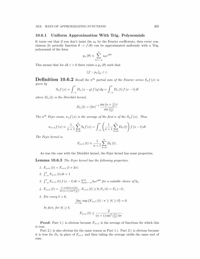
10.6. WAYS OF APPROXIMATING FUNCTIONS 265
10.6.1 Uniform Approximation With Trig. Polynomials
It turns out that if you don’t insist the ak be the Fourier coefficients, then every con-tinuous 2π periodic function θ → f (θ) can be approximated uniformly with a Trig.polynomial of the form
pn (θ) ≡n∑
k=−n
akeikθ
This means that for all ε > 0 there exists a pn (θ) such that
||f − pn||0 < ε.
Definition 10.6.2 Recall the nth partial sum of the Fourier series Snf (x) isgiven by
Snf (x) =
∫ π
−π
Dn (x− y) f (y) dy =
∫ π
−π
Dn (t) f (x− t) dt
where Dn (t) is the Dirichlet kernel,
Dn (t) = (2π)−1 sin
(n+ 1
2
)t
sin(t2
)The nth Fejer mean, σnf (x) is the average of the first n of the Snf (x). Thus
σn+1f (x) ≡1
n+ 1
n∑k=0
Skf (x) =
∫ π
−π
(1
n+ 1
n∑k=0
Dk (t)
)f (x− t) dt
The Fejer kernel is
Fn+1 (t) ≡1
n+ 1
n∑k=0
Dk (t) .
As was the case with the Dirichlet kernel, the Fejer kernel has some properties.
Lemma 10.6.3 The Fejer kernel has the following properties.
1. Fn+1 (t) = Fn+1 (t+ 2π)
2.∫ π
−πFn+1 (t) dt = 1
3.∫ π
−πFn+1 (t) f (x− t) dt =
∑nk=−n bke
ikθ for a suitable choice of bk.
4. Fn+1 (t) =1−cos((n+1)t)
4π(n+1) sin2( t2 ), Fn+1 (t) ≥ 0, Fn (t) = Fn (−t) .
5. For every δ > 0,limn→∞
sup {Fn+1 (t) : π ≥ |t| ≥ δ} = 0.
In fact, for |t| ≥ δ,Fn+1 (t) ≤
2
(n+ 1) sin2(δ2
)4π.
Proof: Part 1.) is obvious because Fn+1 is the average of functions for which thisis true.
Part 2.) is also obvious for the same reason as Part 1.). Part 3.) is obvious becauseit is true for Dn in place of Fn+1 and then taking the average yields the same sort ofsum.
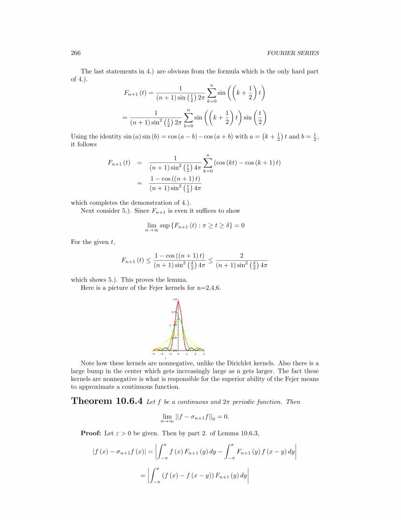
266 FOURIER SERIES
The last statements in 4.) are obvious from the formula which is the only hard partof 4.).
Fn+1 (t) =1
(n+ 1) sin(t2
)2π
n∑k=0
sin
((k +
1
2
)t
)
=1
(n+ 1) sin2(t2
)2π
n∑k=0
sin
((k +
1
2
)t
)sin
(t
2
)Using the identity sin (a) sin (b) = cos (a− b)−cos (a+ b) with a =
(k + 1
2
)t and b = t
2 ,it follows
Fn+1 (t) =1
(n+ 1) sin2(t2
)4π
n∑k=0
(cos (kt)− cos (k + 1) t)
=1− cos ((n+ 1) t)
(n+ 1) sin2(t2
)4π
which completes the demonstration of 4.).Next consider 5.). Since Fn+1 is even it suffices to show
limn→∞
sup {Fn+1 (t) : π ≥ t ≥ δ} = 0
For the given t,
Fn+1 (t) ≤1− cos ((n+ 1) t)
(n+ 1) sin2(δ2
)4π≤ 2
(n+ 1) sin2(δ2
)4π
which shows 5.). This proves the lemma.Here is a picture of the Fejer kernels for n=2,4,6.
2−3
y
t
3−1
0.25
0.5
1.0
0.010
0.75
−2
Note how these kernels are nonnegative, unlike the Dirichlet kernels. Also there is alarge bump in the center which gets increasingly large as n gets larger. The fact thesekernels are nonnegative is what is responsible for the superior ability of the Fejer meansto approximate a continuous function.
Theorem 10.6.4 Let f be a continuous and 2π periodic function. Then
limn→∞
||f − σn+1f ||0 = 0.
Proof: Let ε > 0 be given. Then by part 2. of Lemma 10.6.3,
|f (x)− σn+1f (x)| =∣∣∣∣∫ π
−π
f (x)Fn+1 (y) dy −∫ π
−π
Fn+1 (y) f (x− y) dy∣∣∣∣
=
∣∣∣∣∫ π
−π
(f (x)− f (x− y))Fn+1 (y) dy
∣∣∣∣
10.6. WAYS OF APPROXIMATING FUNCTIONS 267
≤∫ π
−π
|f (x)− f (x− y)|Fn+1 (y) dy
=
∫ δ
−δ
|f (x)− f (x− y)|Fn+1 (y) dy +
∫ π
δ
|f (x)− f (x− y)|Fn+1 (y) dy
+
∫ −δ
−π
|f (x)− f (x− y)|Fn+1 (y) dy
Since Fn+1 is even and |f | is continuous and periodic, hence bounded by some constantM the above is dominated by
≤∫ δ
−δ
|f (x)− f (x− y)|Fn+1 (y) dy + 4M
∫ π
δ
Fn+1 (y) dy
Now choose δ such that for all x, it follows that if |y| < δ then
|f (x)− f (x− y)| < ε/2.
This can be done because f is uniformly continuous on [−π, π] by Theorem 6.8.2 onPage 117. Since it is periodic, it must also be uniformly continuous on R. (why?)Therefore, for this δ, this has shown that for all x
|f (x)− σn+1f (x)| ≤ ε/2 + 4M
∫ π
δ
Fn+1 (y) dy
and now by Lemma 10.6.3 it follows
||f − σn+1f ||0 ≤ ε/2 +8Mπ
(n+ 1) sin2(δ2
)4π
< ε
provided n is large enough. This proves the theorem.
10.6.2 Mean Square Approximation
The partial sums of the Fourier series of f do a better job approximating f in themean square sense than any other linear combination of the functions, eikθ for |k| ≤ n.This will be shown next. It is nothing but a simple computation. Recall the Fouriercoefficients are
ak =1
2π
∫ π
−π
f (θ) e−ikθ
Then using this fact as needed, consider the following computation.∫ π
−π
∣∣∣∣∣f (θ)−n∑
k=−n
bkeikθ
∣∣∣∣∣2
dθ
=
∫ π
−π
(f (θ)−
n∑k=−n
bkeikθ
)(f (θ)−
n∑l=−n
ale−ilθ
)dθ
=
∫ π
−π
(|f (θ)|2 +
(n∑
k=−n
bkeikθ
)(n∑
l=−n
ble−ilθ
)
−f (θ)n∑
l=−n
ble−ilθ − f (θ)
n∑k=−n
bkeikθ
)dθ

268 FOURIER SERIES
=
∫ π
−π
|f (θ)|2 dθ +∑kl
bkbl
∫ π
−π
eikθe−ilθdθ − 2π∑l
blal − 2π∑k
bkak
Then adding and subtracting 2π∑
k |ak|2,
=
∫ π
−π
|f (θ)|2 dθ − 2π∑k
|ak|2 + 2π∑k
|bk|2
−2π∑l
blal − 2π∑k
bkak + 2π∑k
|ak|2
=
∫ π
−π
|f (θ)|2 dθ − 2π∑k
|ak|2 + 2π
(∑k
(bk − ak)(bk − ak
))
=
∫ π
−π
|f (θ)|2 dθ − 2π∑k
|ak|2 + 2π∑k
|bk − ak|2
Therefore, to make ∫ π
−π
∣∣∣∣∣f (θ)−n∑
k=−n
bkeikθ
∣∣∣∣∣2
dθ
as small as possible for all choices of bk, one should let bk = ak, the kth Fourier coefficient.
Stated another way,∫ π
−π
∣∣∣∣∣f (θ)−n∑
k=−n
bkeikθ
∣∣∣∣∣2
dθ ≥∫ π
−π
|f (θ)− Snf (θ)|2 dθ
for any choice of bk. In particular,∫ π
−π
|f (θ)− σn+1f (θ)|2 dθ ≥∫ π
−π
|f (θ)− Snf (θ)|2 dθ. (10.23)
Also, ∫ π
−π
f (θ)Snf (θ)dθ =
∫ π
−π
n∑k=−n
akf (θ) e−ikθdθ
=n∑
k=−n
ak
=2πak︷ ︸︸ ︷∫ π
−π
f (θ) e−ikθdθ
= 2πn∑
k=−n
|ak|2
Similarly, ∫ π
−π
f (θ)Snf (θ) dθ = 2π
n∑k=−n
|ak|2
and a simple computation of the above sort shows that also∫ π
−π
Snf (θ)Snf (θ)dθ = 2π
n∑k=−n
|ak|2 .
Therefore,
0 ≤∫ π
−π
(f (θ)− Snf (θ))(f (θ)− Snf (θ)
)dθ

10.6. WAYS OF APPROXIMATING FUNCTIONS 269
=
∫ π
−π
|f (θ)|2 + |Snf (θ)|2 − f (θ)Snf (θ)− f (θ)Snf (θ)dθ
=
∫ π
−π
|f (θ)|2 − |Snf (θ)|2 dθ
showing
2πn∑
k=−n
|ak|2 ≤∫ π
−π
|Snf (θ)|2 dθ ≤∫ π
−π
|f (θ)|2 dθ (10.24)
Now it is easy to prove the following fundamental theorem.
Theorem 10.6.5 Let f ∈ R ([−π, π]) and it is periodic of period 2π. Then
limn→∞
∫ π
−π
|f − Snf |2 dx = 0.
Proof: First assume f is continuous and 2π periodic. Then by 10.23∫ π
−π
|f − Snf |2 dx ≤∫ π
−π
|f − σn+1f |2 dx
≤∫ π
−π
||f − σn+1f ||20 dx = 2π ||f − σn+1f ||20
and the last expression converges to 0 by Theorem 10.6.4.Next suppose f ∈ R ([−π, π]) and |f (x)| < M for all x. Then the construction used
in Lemma 10.3.2 yields a continuous function h which vanishes off some closed intervalcontained in (−π, π) such that
ε
32M2>
∫ π
−π
|f (x)− h (x)| dx ≥ 1
2M
∫ π
−π
|f (x)− h (x)|2 dx. (10.25)
Since h vanishes off some closed interval contained in (−π, π) , if h is extended off [−π, π]to be 2π periodic, it follows the resulting function, still denoted by h, is continuous. Thenusing the inequality (For a better inequality, see Problem 2.)
(a+ b+ c)2 ≤ 4
(a2 + b2 + c2
)∫ π
−π
|f − Snf |2 dx =
∫ π
−π
(|f − h|+ |h− Snh|+ |Snh− Snf |)2 dx
≤ 4
∫ π
−π
(|f − h|2 + |h− Snh|2 + |Snh− Snf |2
)dx
and from 10.24 and 10.25 this is no larger than
8
∫ π
−π
|f − h|2 dx+ 4
∫ π
−π
|h− Snh|2 dx
< 16Mε
16M+ 4
∫ π
−π
|h− Snh|2 dx
= ε+ 4
∫ π
−π
|h− Snh|2 dx
and by the first part, this last term converges to 0 as n → ∞. Therefore, since ε isarbitrary, this shows that for n large enough,∫ π
−π
|f − Snf |2 dx < ε
This proves the theorem.

270 FOURIER SERIES
10.7 Exercises
1. Suppose f has infinitely many derivatives and is also periodic with period 2π. Letthe Fourier series of f be
∞∑k=−∞
akeikθ
Show that
limk→∞
kmak = limk→∞
kma−k = 0
for every m ∈ N.
2. The proof of Theorem 10.6.5 used the inequality (a+ b+ c)2 ≤ 4
(a2 + b2 + c2
)whenever a, b and c are nonnegative numbers. In fact the 4 can be replaced with3. Show this is true.
3. Let f be a continuous function defined on [−π, π]. Show there exists a polynomial,p such that ||p− f || < ε where
||g|| ≡ sup {|g (x)| : x ∈ [−π, π]} .
Extend this result to an arbitrary interval. This is another approach to the Weier-strass approximation theorem. Hint: First find a linear function ax+ b = y suchthat f − y has the property that it has the same value at both ends of [−π, π].Therefore, you may consider this as the restriction to [−π, π] of a continuousperiodic function F . Now find a trig polynomial,
σ (x) ≡ a0 +n∑
k=1
ak cos kx+ bk sin kx
such that ||σ − F || < ε3 . Recall 10.4. Now consider the power series of the trig
functions making use of the error estimate for the remainder after m terms.
4. The inequality established above,
2π
n∑k=−n
|ak|2 ≤∫ π
−π
|Snf (θ)|2 dθ ≤∫ π
−π
|f (θ)|2 dθ
is called Bessel’s inequality. Use this inequality to give an easy proof that for allf ∈ R ([−π, π]) ,
limn→∞
∫ π
−π
f (x) einxdx = 0.
Recall that in the Riemann Lebesgue lemma |f | ∈ R ((a, b]) so while this exerciseis easier, it lacks the generality of the earlier proof.
5. Suppose f (x) = X[a,b] (x) . Show
limα→∞
∫ b
a
f (x) sin (αx+ β) dx = 0.
Use this to construct a much simpler proof of the Riemann Lebesgue lemma thanthat given in the chapter. Hint: Show it works for f a step function and thenobtain the conclusion for |f | ∈ R ((a, b]) .

10.7. EXERCISES 271
6. Let f (x) = x for x ∈ (−π, π) and extend to make the resulting function definedon R and periodic of period 2π. Find the Fourier series of f . Verify the Fourierseries converges to the midpoint of the jump and use this series to find a niceformula for π
4 . Hint: For the last part consider x = π2 .
7. Let f (x) = x2 on (−π, π) and extend to form a 2π periodic function defined on
R. Find the Fourier series of f . Now obtain a famous formula for π2
6 by lettingx = π.
8. Let f (x) = cosx for x ∈ (0, π) and define f (x) ≡ − cosx for x ∈ (−π, 0). Nowextend this function to make it 2π periodic. Find the Fourier series of f .
9. Suppose f, g ∈ R ([−π, π]). Show
1
2π
∫ π
−π
fgdx =∞∑
k=−∞
αkβk,
where αk are the Fourier coefficients of f and βk are the Fourier coefficients of g.
10. Recall the partial summation formula, called the Dirichlet formula which says that
q∑k=p
akbk = Aqbq −Ap−1bp +
q−1∑k=p
Ak (bk − bk+1) .
Here Aq ≡∑q
k=1 ak. Also recall Dirichlet’s test which says that if limk→∞ bk = 0,Ak are bounded, and
∑|bk − bk+1| converges, then
∑akbk converges. Show the
partial sums of∑
k sin kx are bounded for each x ∈ R. Using this fact and theDirichlet test above, obtain some theorems which will state that
∑k ak sin kx
converges for all x.
11. Let {an} be a sequence of positive numbers having the property that limn→∞ nan =0 and for all n ∈ N, nan ≥ (n+ 1) an+1. Show that if this is so, it follows thatthe series,
∑∞k=1 an sinnx converges uniformly on R. This is a variation of a very
interesting problem found in Apostol’s book, [3]. Hint: Use the Dirichlet formulaof Problem 10 on
∑kak
sin kxk and show the partial sums of
∑sin kx
k are boundedindependent of x. To do this, you might argue the maximum value of the partialsums of this series occur when
∑nk=1 cos kx = 0. Sum this series by considering
the real part of the geometric series,∑q
k=1
(eix)k
and then show the partial sums
of∑
sin kxk are Riemann sums for a certain finite integral.
12. The problem in Apostol’s book mentioned in Problem 11 does not require nanto be decreasing and is as follows. Let {ak}∞k=1 be a decreasing sequence of non-negative numbers which satisfies limn→∞ nan = 0. Then
∞∑k=1
ak sin (kx)
converges uniformly on R. You can find this problem worked out completely inJones [21]. Fill in the details to the following argument or something like it toobtain a proof. First show that for p < q, and x ∈ (0, π) ,∣∣∣∣∣∣
q∑k=p
ak sin (kx)
∣∣∣∣∣∣ ≤ 3ap csc(x2
). (10.26)
272 FOURIER SERIES
To do this, use summation by parts using the formula
q∑k=p
sin (kx) =cos((p− 1
2
)x)− cos
((q + 1
2
)x)
2 sin(x2
) ,
which you can establish by taking the imaginary part of a geometric series of
the form∑q
k=1
(eix)k
or else the approach used above to find a formula for theDirichlet kernel. Now define
b (p) ≡ sup {nan : n ≥ p} .
Thus b (p) → 0, b (p) is decreasing in p, and if k ≥ n, ak ≤ b (n) /k. Then from10.26 and the assumption {ak} is decreasing,
∣∣∣∣∣∣q∑
k=p
ak sin (kx)
∣∣∣∣∣∣ ≤∣∣∣∣∣∣
m∑k=p
ak sin (kx)
∣∣∣∣∣∣+≡0 if m=q︷ ︸︸ ︷∣∣∣∣∣
q∑k=m+1
ak sin (kx)
∣∣∣∣∣≤
{ ∑mk=p
b(k)k |sin (kx)|+ 3ap csc
(x2
)if m < q∑q
k=pb(k)k |sin (kx)| if m = q.
≤
{ ∑mk=p
b(k)k kx+ 3ap
2πx if m < q∑q
k=pb(k)k kx if m = q
(10.27)
where this uses the inequalities
sin(x2
)≥ x
2π, |sin (x)| ≤ |x| for x ∈ (0, π) .
There are two cases to consider depending on whether x ≤ 1/q. First supposethat x ≤ 1/q. Then let m = q and use the bottom line of 10.27 to write that inthis case, ∣∣∣∣∣∣
q∑k=p
ak sin (kx)
∣∣∣∣∣∣ ≤ 1
q
q∑k=p
b (k) ≤ b (p) .
If x > 1/q, then q > 1/x and you use the top line of 10.27 picking m such that
q >1
x≥ m ≥ 1
x− 1.
Then in this case,∣∣∣∣∣∣q∑
k=p
ak sin (kx)
∣∣∣∣∣∣ ≤m∑
k=p
b (k)
kkx+ 3ap
2π
x
≤ b (p)x (m− p) + 6πap (m+ 1)
≤ b (p)x
(1
x
)+ 6π
b (p)
m+ 1(m+ 1) ≤ 25b (p) .
Therefore, the partial sums of the series,∑ak sin kx form a uniformly Cauchy
sequence and must converge uniformly on (0, π). Now explain why this impliesthe series converges uniformly on R.
13. Suppose f (x) =∑∞
k=1 ak sin kx and that the convergence is uniform. Recallsomething like this holds for power series. Is it reasonable to suppose that f ′ (x) =∑∞
k=1 akk cos kx? Explain.
10.7. EXERCISES 273
14. Suppose |uk (x)| ≤ Kk for all x ∈ D where
∞∑k=−∞
Kk = limn→∞
n∑k=−n
Kk <∞.
Show that∑∞
k=−∞ uk (x) converges converges uniformly on D in the sense thatfor all ε > 0, there exists N such that whenever n > N ,∣∣∣∣∣
∞∑k=−∞
uk (x)−n∑
k=−n
uk (x)
∣∣∣∣∣ < ε
for all x ∈ D. This is called the Weierstrass M test.
15. Let ak, bk ≥ 0. Show the Cauchy Schwarz inequality
n∑k=1
akbk ≤
(n∑
k=1
a2k
)1/2( n∑k=1
b2k
)1/2
To do this note that
p (t) ≡n∑
k=1
(ak + tbk)2 ≥ 0
for all t. Now pick an auspicious value of t, perhaps the value at which p (t) achievesits minimum.
16. Suppose f is a differentiable function of period 2π and suppose that both f andf ′ are in R ([−π, π]) such that for all x ∈ (−π, π) and y sufficiently small,
f (x+ y)− f (x) =∫ x+y
x
f ′ (t) dt.
Show that the Fourier series of f converges uniformly to f . Hint: First show usingthe Dini criterion that Snf (x) → f (x) for all x. Next let
∑∞k=−∞ ake
ikx be the
Fourier series for f . Then from the definition of ak, show that for k = 0, ak = 1ika
′k
where a′k is the Fourier coefficient of f ′. Now use the Bessel’s inequality to argue
that∑∞
k=−∞ |a′k|2< ∞ and then show this implies
∑|ak| < ∞. You might
want to use the Cauchy Schwarz inequality in Problem 15 to do this part. Thenusing the version of the Weierstrass M test given in Problem 14 obtain uniformconvergence of the Fourier series to f .
17. Let f be a function defined on R. Then f is even if f (θ) = f (−θ) for all θ ∈ R.Also f is called odd if for all θ ∈ R, −f (θ) = f (−θ). Now using the Weierstrassapproximation theorem show directly that if h is a continuous even 2π periodicfunction, then for every ε > 0 there exists an m and constants, a0, · · · , am suchthat ∣∣∣∣∣h (θ)−
m∑k=0
ak cosk (θ)
∣∣∣∣∣ < ε
for all θ ∈ R. Hint: Note the function arccos is continuous and maps [−1, 1]onto [0, π] . Using this show you can define g a continuous function on [−1, 1] byg (cos θ) = h (θ) for θ on [0, π]. Now use the Weierstrass approximation theoremon [−1, 1].

274 FOURIER SERIES
18. Show that if f is any odd 2π periodic function, then its Fourier series can besimplified to an expression of the form
∞∑n=1
bn sin (nx)
and also f (mπ) = 0 for all m ∈ N.
19. Consider the symbol∑∞
k=1 an. The infinite sum might not converge. Summabilitymethods are systematic ways of assigning a number to such a symbol. The nth
Ceasaro mean σn is defined as the average of the first n partial sums of the series.Thus
σn ≡1
n
n∑k=1
Sk
where
Sk ≡k∑
j=1
aj .
Show that if∑∞
k=1 an converges then limn→∞ σn also exists and equals the samething. Next find an example where, although
∑∞k=1 an fails to converge, limn→∞ σn
does exist. This summability method is called Ceasaro summability. Recall theFejer means were obtained in just this way.
20. Let 0 < r < 1 and for f a periodic function of period 2π where f ∈ R ([−π, π]) ,consider
Arf (θ) ≡∞∑
k=−∞
r|k|akeikθ
where the ak are the Fourier coefficients of f. Show that if f is continuous, then
limr→1−
Arf (θ) = f (θ) .
Hint: You need to find a kernel and write as the integral of the kernel convolvedwith f . Then consider properties of this kernel as was done with the Fejer kernel.In carrying out the details, you need to verify the convergence of the series isuniform in some sense in order to switch the sum with an integral.
21. Recall the Dirichlet kernel is
Dn (t) ≡ (2π)−1 sin
(n+ 1
2
)t
sin(t2
)and it has the property that
∫ π
−πDn (t) dt = 1. Show first that this implies
1
2π
∫ π
−π
sin (nt) cos (t/2)
sin (t/2)dt = 1
and this implies1
π
∫ π
0
sin (nt) cos (t/2)
sin (t/2)= 1.
Next change the variable to show the integral equals
1
π
∫ nπ
0
sin (u) cos (u/2n)
sin (u/2n)
1
ndu

10.7. EXERCISES 275
Now show that
limn→∞
sin (u) cos (u/2n)
sin (u/2n)
1
n=
2 sinu
u
Next show that
limn→∞
1
π
∫ nπ
0
2 sinu
udu = lim
n→∞
1
π
∫ nπ
0
sin (u) cos (u/2n)
sin (u/2n)
1
ndu = 1
Finally show
limR→∞
∫ R
0
sinu
udu =
π
2≡∫ π
0
sinu
udu
This is a very important improper integral.
22. To work this problem, you should first review Problem 25 on Page 246 aboutinterchanging the order of iterated integrals. Suppose f is Riemann integrable onevery finite interval, bounded, and
limR→∞
∫ R
0
|f (t)| dt <∞, limR→∞
∫ 0
−R
|f (t)| dt <∞.
Show that
limR→∞
∫ R
0
f (t) eistdt, limR→∞
∫ 0
−R
f (t) e−itsdt
both exist. Define
limR→∞
∫ R
0
f (t) eistdt ≡∫ ∞
0
f (t) e−itsdt
limR→∞
∫ 0
−R
f (t) e−itsdt ≡∫ 0
−∞f (t) e−itsdt
and ∫ ∞
−∞f (t) e−istdt ≡
∫ ∞
0
f (t) e−itsdt+
∫ 0
−∞f (t) e−itsdt
Now suppose the Dini condition on f, that
t→ f (x− t) + f (x+ t)− (f (x−) + f (x+))
2t
is a function in R ((0, 1]) . This happens, for example if for t > 0 and small,
|f (x+ t)− f (x+)| ≤ Ctθ for θ > 0
and if|f (x− t)− f (x−)| ≤ Ctα for α > 0
Now show using Problem 25 on Page 246 (You fill in the details including modi-fying things so that the result of this problem applies.) to conclude
1
2π
∫ R
−R
∫ ∞
−∞f (t) e−itsdteisxds =
1
2π
∫ R
−R
∫ ∞
−∞f (x− u) eisududs
=1
2π
∫ ∞
−∞f (x− u)
∫ R
−R
eisudsdu =1
π
∫ ∞
−∞f (x− u) sinRu
udu
=2
π
∫ ∞
0
sinu
u
f(x− u
R
)+ f
(x+ u
R
)2
du

276 FOURIER SERIES
Conclude using Problem 21
1
2π
∫ R
−R
∫ ∞
−∞f (t) e−itsdteisxds− f (x−) + f (x+)
2(10.28)
=2
π
∫ ∞
0
sinu
u
(f(x− u
R
)+ f
(x+ u
R
)2
− f (x−) + f (x+)
2
)du
Explain how the above equals an expression of the form
2
π
∫ R
0
sinu
u
(f(x− u
R
)+ f
(x+ u
R
)2
− f (x−) + f (x+)
2
)du+ e (R)
where e (R) → 0 as R → ∞. Now change the variable letting u/R = t andconclude 10.28 equals
2
π
∫ 1
0
sin (Rt)
(f (x− t) + f (x+ t)− (f (x−) + f (x+))
2t
)dt+ e (R)
Now apply the Riemann Lebesgue lemma to conclude
limR→∞
1
2π
∫ R
−R
∫ ∞
−∞f (t) e−itsdteisxds =
f (x−) + f (x+)
2.
The Fourier transform is defined as
F (s) ≡ 1√2π
∫ ∞
−∞f (t) e−itsdt
and this has shown that under the Dini condition described above and for the sortof f defined above,
f (x−) + f (x+)
2= lim
R→∞
1
2π
∫ R
−R
F (s) eisxds
This is the Fourier inversion formula.

The Generalized RiemannIntegral
11.1 Definitions And Basic Properties
This chapter is on the generalized Riemann integral. The Riemann Darboux integralpresended earlier has been obsolete for over 100 years. The integral of this chapter iscertainly not obsolete and is in certain important ways the very best integral currentlyknown. This integral is called the generalized Riemann integral, also the HenstockKurzweil integral after the two people who invented it and sometimes the gauge integral.Other books which discuss this integral are the books by Bartle [5], Bartle and Sherbert,[6], Henstock [19], or McLeod [26]. Considerably more is presented in these references.In what follows, F will be an increasing function, the most important example beingF (x) = x.
Definition 11.1.1 Let [a, b] be a closed and bounded interval. A tagged divi-sion1 of [a, b] = I is a set of the form P ≡ {(Ii, ti)}ni=1 where ti ∈ Ii = [xi−1, xi], anda = xi−1 < · · · < xn = b. Let the ti be referred to as the tags. A function δ : I → (0,∞)is called a gauge function or simply gauge for short. A tagged division, P is called δfine if
Ii ⊆ [ti − δ (ti) , ti + δ (ti)] .
A δ fine division, is understood to be tagged. More generally, a collection, {(Ii, ti)}pi=1
is δ fine if the above inclusion holds for each of these intervals and their interiors aredisjoint even if their union is not equal to the whole interval, [a, b].
The following fundamental result is essential.
Proposition 11.1.2 Let [a, b] be an interval and let δ be a gauge function on [a, b].Then there exists a δ fine tagged division of [a, b].
Proof:Suppose not. Then one of[a, a+b
2
]or[a+b2 , b
]must fail to have a δ fine
tagged division because if they both had such a δ fine division, the union of the two δfine divisions would be a δ fine division of [a, b]. Denote by I1 the interval which doesnot have a δ fine division. Then repeat the above argument, dividing I1 into two equalintervals and pick the one, I2 which fails to have a δ fine division. Continue this way toget a nested sequence of closed intervals, {Ii} having the property that each interval inthe set fails to have a δ fine division and diam (Ii)→ 0. Therefore,
∩∞i=1Ii = {x}1In beginning calculus books, this is often called a partition. The word, division is a much better
word to use. what the xi do is to “divide” the interval into little subintervals.
277

278 THE GENERALIZED RIEMANN INTEGRAL
where x ∈ [a, b]. Now [x− δ (x) , x+ δ (x)] must contain some Ik because the diametersof these intervals converge to zero. It follows that {(Ik, x)} is a δ fine division of Ik,contrary to the construction which required that none of these intervals had a δ finedivision. This proves the proposition.
With this proposition and definition, it is time to define the generalized Riemannintegral. The functions being integrated typically have values in R or C but there isno reason to restrict to this situation and so in the following definition, X will denotethe space in which f has its values. For example, X could be Rp which becomesimportant in multivariable calculus. For now, just think R if you like. It will be assumedCauchy sequences converge and there is something like the absolute value, called a normalthough it is possible to generalize even further.
Definition 11.1.3 Let X be a complete normed vector space. (For example,X = R or X = C or X = Rp.) Then f : [a, b] → X is generalized Riemann integrable,written as f ∈ R∗ [a, b] if there exists R ∈ X such that for all ε > 0, there exists agauge, δ, such that if P ≡ {(Ii, ti)}ni=1 is δ fine then defining, S (P, f) by
S (P, f) ≡n∑
i=1
f (ti)∆Fi,
where if Ii = [xi−1, xi] ,∆Fi ≡ F (xi)− F (xi−1)
it follows|S (P, f)−R| < ε.
Then ∫I
fdF ≡∫ b
a
fdF ≡ R.
Here |·| refers to the norm on X for R this is just the absolute value.
Note that if P is δ1 fine and δ1 ≤ δ then it follows P is also δ fine.How does this relate to the usual Riemann integral discussed above in Theorem 9.4.2
and the definition of the Riemann integral given before this?To begin with, is there a way to tell whether a given function is in R∗ [a, b]? The
following Cauchy criterion is useful to make this determination.
Proposition 11.1.4 A function f : [a, b]→ X is in R∗ [a, b] if and only if for everyε > 0, there exists a gauge function δε such that if P and Q are any two divisions whichare δε fine, then
|S (P, f)− S (Q, f)| < ε.
Proof:Suppose first that f ∈ R∗ [a, b]. Then there exists a gauge, δε, and an elementof X, R, such that if P is δε fine, then
|R− S (P, f)| < ε/2.
Now let P,Q be two such δε fine divisions. Then
|S (P, f)− S (Q, f)| ≤ |S (P, f)−R|+ |R− S (Q, f)|
<ε
2+ε
2= ε.
Conversely, suppose the condition of the proposition holds. Let εn → 0+ as n→∞and let δεn denote the gauge which goes with εn. Without loss of generality, assume

11.1. DEFINITIONS AND BASIC PROPERTIES 279
that δεn is decreasing in n. Let Rεn denote the closure of all the sums, S (P, f) where Pis δεn fine. From the condition, it follows diam (Rεn) ≤ εn and that these closed sets arenested in the sense that Rεn ⊇ Rεn+1 because δεn is decreasing in n. Therefore, thereexists a unique, R ∈ ∩∞n=1Rεn . To see this, let rn ∈ Rεn . Then since the diameters ofthe Rεn are converging to 0, {rn} is a Cauchy sequence which must converge to someR ∈ X. Since Rεn is closed, it follows R ∈ Rεn for each n. Letting ε > 0 be given, thereexists εn < ε and for P a δεn fine division,
|S (P, f)−R| ≤ εn < ε.
Therefore, R =∫If . This proves the proposition.
Are there examples of functions which are in R∗ [a, b]? Are there examples of func-tions which are not? It turns out the second question is harder than the first althoughit is very easy to answer this question in the case of the obsolete Riemann integral. Thegeneralized Riemann integral is a vastly superior integral which can integrate a veryimpressive collection of functions. Consider the first question. Recall the definition ofthe Riemann integral given above which is listed here for convenience.
Definition 11.1.5 A bounded function f defined on [a, b] is said to be RiemannStieltjes integrable if there exists a number, I with the property that for every ε > 0,there exists δ > 0 such that if
P ≡ {x0, x1, · · · , xn}
is any partition having ||P || < δ, and zi ∈ [xi−1, xi] ,∣∣∣∣∣I −n∑
i=1
f (zi) (F (xi)− F (xi−1))
∣∣∣∣∣ < ε.
The number∫ b
af (x) dF is defined as I.
First note that if δ > 0 and if every interval in a division has length less than δ thenthe division is δ fine. In fact, you could pick the tags as any point in the intervals. Thenthe following theorem follows immediately.
Theorem 11.1.6 Let f be Riemann Stieltjes integrable according to Definition11.1.5. Then f is generalized Riemann integrable and the integrals are the same.
Proof: Just let the gauge functions be constant functions.In particular, the following important theorem follows from Theorem 9.4.6.
Theorem 11.1.7 Let f be continuous on [a, b] and let F be any increasing in-tegrator. Then f ∈ R∗ [a, b] .
Many functions other than continuous ones are integrable however. In fact, it isfairly difficult to come up with easy examples because this integral can integrate almostanything you can imagine, including the function which equals 1 on the rationals and 0on the irrationals which is not Riemann integrable. This will be shown later.
The integral is linear. This will be shown next.
Theorem 11.1.8 Suppose α and β are constants and that f and g are inR∗ [a, b]. Then αf + βg ∈ R∗ [a, b] and∫
I
(αf + βg) dF = α
∫I
fdF + β
∫I
gdF.
280 THE GENERALIZED RIEMANN INTEGRAL
Proof:Let η = ε|β|+|α|+1 and choose gauges, δg and δf such that if P is δg fine,∣∣∣∣S (P, g)−
∫I
gdF
∣∣∣∣ < η
and that if P is δf fine, ∣∣∣∣S (P, f)−∫I
fdF
∣∣∣∣ < η.
Now let δ = min (δg, δf ). Then if P is δ fine the above inequalities both hold. Therefore,from the definition of S (P, f),
S (P, αf + βg) = αS (P, f) + βS (P, g)
and so ∣∣∣∣S (P, αf + βg)−(β
∫I
gdF + α
∫I
fdF
)∣∣∣∣ ≤ ∣∣∣∣βS (P, g)− β∫I
gdF
∣∣∣∣+
∣∣∣∣αS (P, f)− α∫I
fdF
∣∣∣∣ ≤ |β| η + |α| η < ε.
Since ε > 0 is arbitrary, this shows the number, β∫IgdF + α
∫IfdF qualifies in the
definition of the generalized Riemann integral and so αf + βg ∈ R∗ [a, b] and∫I
(αf + βg) dF = β
∫I
gdF + α
∫I
fdF.
The following lemma is also very easy to establish from the definition.
Lemma 11.1.9 If f ≥ 0 and f ∈ R∗ [a, b], then∫IfdF ≥ 0. Also, if f has complex
values and is in R∗ [I], then both Re f and Im f are in R∗ [I].
Proof: To show the first part, let ε > 0 be given and let δ be a gauge function suchthat if P is δ fine then ∣∣∣∣S (f, P )−
∫I
fdF
∣∣∣∣ ≤ ε.Since F is increasing, it is clear that S (f, P ) ≥ 0. Therefore,∫
I
fdF ≥ S (f, P )− ε ≥ −ε
and since ε is arbitrary, it follows∫IfdF ≥ 0 as claimed.
To verify the second part, note that by Proposition 11.1.4 there exists a gauge, δsuch that if P,Q are δ fine then
|S (f, P )− S (f,Q)| < ε
But
|S (Re f, P )− S (Re f,Q)| = |Re (S (f, P ))− Re (S (f,Q))|≤ |S (f, P )− S (f,Q)|
and so the conditions of Proposition 11.1.4 are satisfied and you can conclude Re f ∈R∗ [I] . Similar reasoning applies to Im f. This proves the lemma.

11.1. DEFINITIONS AND BASIC PROPERTIES 281
Corollary 11.1.10 If |f | , f ∈ R∗ [a, b], where f has values in C, then∣∣∣∣∫I
fdF
∣∣∣∣ ≤ ∫I
|f | dF.
Proof:Let |α| = 1 and α∫IfdF =
∣∣∫IfdF
∣∣. Then by Theorem 11.1.8 and Lemma11.1.9, ∣∣∣∣∫
I
fdF
∣∣∣∣ =
∫I
αfdF =
∫I
(Re (αf) + i Im (αf)) dF
=
∫I
Re (αf) dF + i
∫I
Im (αf) dF =
∫I
Re (αf) dF
≤∫I
|Re (αf)| dF ≤∫I
|f | dF
Note the assumption that |f | ∈ R∗ [a, b].The following lemma is also fundamental.
Lemma 11.1.11 If f ∈ R∗ [a, b] and [c, d] ⊆ [a, b], then f ∈ R∗ [c, d].
Proof:Let ε > 0 and choose a gauge δ such that if P is a division of [a, b] which isδ fine, then
|S (P, f)−R| < ε/2.
Now pick a δ fine division of [c, d] , {(Ii, ti)}li=r and then let {(Ii, ti)}r−1i=1 and {(Ii, ti)}ni=l+1
be fixed δ fine divisions on [a, c] and [d, b] respectively.Now let P1 and Q1 be δ fine divisions of [c, d] and let P and Q be the respective δ
fine divisions if [a, b] just described which are obtained from P1 and Q1 by adding in
{(Ii, ti)}r−1i=1 and {(Ii, ti)}ni=l+1. Then
ε > |S (Q, f)− S (P, f)| = |S (Q1, f)− S (P1, f)| .
By the above Cauchy criterion, Proposition 11.1.4, f ∈ R∗ [c, d] as claimed.
Corollary 11.1.12 Suppose c ∈ [a, b] and that f ∈ R∗ [a, b] . Then f ∈ R∗ [a, c] andf ∈ R∗ [c, b]. Furthermore, ∫
I
fdF =
∫ c
a
fdF +
∫ b
c
fdF.
Here∫ c
afdF means
∫[a,c]
fdF .
Proof: Let ε > 0. Let δ1 be a gauge function on [a, c] such that whenever P1 is aδ1 fine division of [a, c], ∣∣∣∣∫ c
a
fdF − S (P1, f)
∣∣∣∣ < ε/3.
Let δ2 be a gauge function on [c, b] such that whenever P2 is a δ2 fine division of [c, b],∣∣∣∣∣∫ b
c
fdF − S (P2, f)
∣∣∣∣∣ < ε/3.
Let δ3 be a gauge function on [a, b] such that if P is a δ3 fine division of [a, b] ,∣∣∣∣∣∫ b
a
fdF − S (P, f)
∣∣∣∣∣ < ε/3.

282 THE GENERALIZED RIEMANN INTEGRAL
Now define a gauge function
δ (x) ≡{
min (δ1, δ3) on [a, c]min (δ2, δ3) on [c, b]
Then letting P1 be a δ fine division on [a, c] and P2 be a δ fine division on [c, b] , itfollows that P = P1∪P2 is a δ3 fine division on [a, b] and all the above inequalities hold.Thus noting that S (P, f) = S (P1, f) + S (P2, f) ,∣∣∣∣∣
∫I
fdF −
(∫ c
a
fdF +
∫ b
c
fdF
)∣∣∣∣∣≤
∣∣∣∣∫I
fdF − (S (P1, f) + S (P2, f))
∣∣∣∣+
∣∣∣∣∣S (P1, f) + S (P2, f)−
(∫ c
a
fdF +
∫ b
c
fdF
)∣∣∣∣∣≤
∣∣∣∣∫I
fdF − S (P, f)
∣∣∣∣+ ∣∣∣∣S (P1, f)−∫ c
a
fdF
∣∣∣∣+∣∣∣∣∣S (P2, f)−
∫ b
c
fdF
∣∣∣∣∣< ε/3 + ε/3 + ε/3 = ε.
Since ε is arbitrary, the conclusion of the corollary follows. This proves the corollary.The following lemma, sometimes called Henstock’s lemma is of great significance.
Lemma 11.1.13 Suppose that f ∈ R∗ [a, b] and that whenever, Q is a δ fine divisionof I, ∣∣∣∣S (Q, f)−
∫I
fdF
∣∣∣∣ ≤ ε.Then if P = {(Ii, ti)}ni=1 is any δ fine division, and P ′ =
{(Iij , tij
)}rj=1
is a subset of
P , then ∣∣∣∣∣∣r∑
j=1
f(tij)∆Fi −
r∑j=1
∫Iij
fdF
∣∣∣∣∣∣ ≤ ε.Proof:Let (Jk, t) ∈ P \ P ′. From Lemma 11.1.11, f ∈ R∗ [Jk]. Therefore, letting
{(Jki, tki)}lki=1 be a suitable δ fine division of Jk,∣∣∣∣∣∫Jk
fdF −lk∑i=1
f (tki)∆Fi
∣∣∣∣∣ < η
where η > 0. Then the collection of these δ fine divisions, {(Jki, tki)}lki=1 taken together
with{(Iij , tij
)}rj=1
forms a δ fine division of I denoted by P . Therefore,
ε ≥∣∣∣∣S (P , f)− ∫
I
fdF
∣∣∣∣ =∣∣∣∣∣∣
r∑j=1
f(tij)∆Fi −
r∑j=1
∫Iij
fdF
+∑
k/∈{i1,··· ,ir}
lk∑i=1
f (tki)∆Fi −∑
k/∈{i1,··· ,ir}
∫Jk
fdF
∣∣∣∣∣∣
11.1. DEFINITIONS AND BASIC PROPERTIES 283
≥
∣∣∣∣∣∣r∑
j=1
f(tij)∆Fi −
r∑j=1
∫Iij
fdF
∣∣∣∣∣∣− |P \ P ′| η
where |P \ P ′| denotes the number of intervals contained in P \ P ′. It follows that
ε+ |P \ P ′| η ≥
∣∣∣∣∣∣r∑
j=1
f(tij)∆Fi −
r∑j=1
∫Iij
fdF
∣∣∣∣∣∣and since η is arbitrary, this proves the lemma.
Consider {(Ij , tj)}pj=1 a subset of a division of [a, b]. If δ is a gauge and {(Ij , tj)}pj=1is δ fine, this can always be considered as a subset of a δ fine division of the wholeinterval and so the following corollary is immediate. It is this corollary which seems ofmost use and may also be referred to as Henstock’s lemma.
Corollary 11.1.14 Suppose that f ∈ R∗ [a, b] and that whenever, Q is a δ finedivision of I, ∣∣∣∣S (Q, f)−
∫I
fdF
∣∣∣∣ ≤ ε.Then if {(Ii, ti)}pi=1 is δ fine, it follows that∣∣∣∣∣∣
p∑j=1
f (tj)∆F (Ij)−p∑
j=1
∫Ij
fdF
∣∣∣∣∣∣ ≤ ε.Here is another corollary in the special case where f has real values.
Corollary 11.1.15 Suppose f ∈ R∗ [a, b] has values in R and that∣∣∣∣S (P, f)−∫I
fdF
∣∣∣∣ ≤ εfor all P which is δ fine. Then if P = {(Ii, ti)}ni=1 is δ fine,
n∑i=1
∣∣∣∣f (ti)∆Fi −∫Ii
fdF
∣∣∣∣ ≤ 2ε. (11.1)
Proof:Let I ≡{i : f (ti)∆Fi ≥
∫IifdF
}and let IC ≡ {1, · · · , n} \ I. Then by
Henstock’s lemma∣∣∣∣∣∑i∈I
f (ti)∆Fi −∑i∈I
∫Ii
fdF
∣∣∣∣∣ =∑i∈I
∣∣∣∣f (ti)∆Fi −∫Ii
fdF
∣∣∣∣ ≤ εand ∣∣∣∣∣∑
i∈IC
f (ti)∆Fi −∑i∈IC
∫Ii
fdF
∣∣∣∣∣ = ∑i∈IC
∣∣∣∣f (ti)∆Fi −∫Ii
fdF
∣∣∣∣ ≤ εso adding these together yields 11.1.
This generalizes immediately to the following.
Corollary 11.1.16 Suppose f ∈ R∗ [a, b] has values in C and that∣∣∣∣S (P, f)−∫I
fdF
∣∣∣∣ ≤ ε (11.2)
284 THE GENERALIZED RIEMANN INTEGRAL
for all P which is δ fine. Then if P = {(Ii, ti)}ni=1 is δ fine,
n∑i=1
∣∣∣∣f (ti)∆Fi −∫Ii
fdF
∣∣∣∣ ≤ 4ε. (11.3)
Proof: It is clear that if 11.2 holds, then∣∣∣∣S (P,Re f)− Re
∫I
fdF
∣∣∣∣ ≤ εwhich shows that Re
∫IfdF =
∫IRe fdF . Similarly Im
∫IfdF =
∫IIm fdF . Therefore,
using Corollary 11.1.15
n∑i=1
∣∣∣∣Re f (ti)∆Fi −∫Ii
Re fdF
∣∣∣∣ ≤ 2ε
andn∑
i=1
∣∣∣∣i Im f (ti)∆Fi −∫Ii
i Im fdF
∣∣∣∣ ≤ 2ε.
Adding and using the triangle inequality, yields 11.3.Next is a version of the monotone convergence theorem. The monotone convergence
theorem is one which says that under suitable conditions, if fn → f pointwise, then∫IfndF →
∫IfdF . These sorts of theorems are not available for the beginning calculus
type of integral. This is one of the reasons for considering the generalized integral. Thefollowing proof is a special case of one presented in McLeod [26].
Theorem 11.1.17 Let fn (x) ≥ 0 and suppose fn ∈ R∗ [a, b] , · · · fn (x) ≤fn+1 (x) · · · and that f (x) = limn→∞ fn (x) for all x and that f (x) has real values.Also suppose that
{∫Ifn}∞n=1
is a bounded sequence. Then f ∈ R∗ [a, b] and∫I
fdF = limn→∞
∫I
fndF (11.4)
Proof:The proof will be based on the following lemma. The conclusion of this lemmais sometimes referred to as equiintegrable.
Lemma 11.1.18 In the situation of Theorem 11.1.17 let ε > 0 be given. Then thereexists a gauge, δ, such that if P is δ fine, then for all n ∈ N,∣∣∣∣S (P, fn)−
∫I
fndF
∣∣∣∣ < ε. (11.5)
Proof of the Lemma: Let 3η + (F (b)− F (a)) η < ε.Claim 1: There exists N ∈ N such that whenever n, j ≥ N∣∣∣∣∫
I
fndF −∫I
fjdF
∣∣∣∣ < η. (11.6)
Proof of Claim 1: Such an N exists because, the sequence,{∫
IfndF
}∞n=1
is increasingand bounded above and is therefore a Cauchy sequence. This proves the claim.
Claim 2: There exists a sequence of disjoint sets, {En}∞n=N such that for x ∈ En,it follows that for all j ≥ n,
|fj (x)− f (x)| < η.

11.1. DEFINITIONS AND BASIC PROPERTIES 285
Proof of Claim 2: For n ≥ N , let
Fn ≡ {x : |fj (x)− f (x)| < η for all j ≥ n} .
Then the sets, Fn are increasing in n and their union equals I. Let EN = FN and letEn = Fn \ Fn−1. Therefore, the En are disjoint and their union equals I. This provesthe claim.
Claim 3: There exists a gauge function δ such that if P = {(Ii, ti)}qi=1 is δ fine andif
Ij ≡ {i : ti ∈ Ej} , Ij ≡ ∅ if j < N,
then if J ⊆ {n, n+ 1, · · · }∣∣∣∣∣∣∑j=J
∑i∈Ij
fn (ti)∆Fi −∑j∈J
∑i∈Ij
∫Ii
fndF
∣∣∣∣∣∣ ≤ η2−n. (11.7)
Proof of Claim 3: First note the sums are not really infinite sums because thereare only finitely many tags. Thus Ij = ∅ for all but finitely many j. Choose gauges,δn, n = 1, 2, · · · such that if P is δn fine, then∣∣∣∣∫
I
fndF − S (P, fn)
∣∣∣∣ < η2−n (11.8)
and define δ on I by letting
δ (x) = min (δ1 (x) , · · · , δp (x)) if x ∈ Ep. (11.9)
Since the union of the En equals I, this defines δ on I. Note that some of the En may beempty. If n ≤ j, then δn (x) got included in the above minimum for all x ∈ Ej , j ∈ J .Therefore, by Corollary 11.1.14, Henstock’s lemma, it follows that 11.7 holds. Thisproves Claim 3.
Suppose now that P = {(Ii, ti)}qi=1 is δ fine. It is desired to verify 11.5. Note first∫I
fndF =∞∑
j=min(n,N)
∑i∈Ij
∫Ii
fndF, S (P, fn) =∞∑
j=min(n,N)
∑i∈Ij
fn (ti)∆Fi
where as before, the sums are really finite. Recall Ij ≡ ∅ if j < N . If n ≤ N, then byClaim 3,
∣∣∣∣∫I
fndF − S (P, f)
∣∣∣∣ =∣∣∣∣∣∣∞∑j=n
∑i∈Ij
∫Ii
fndF −∞∑j=n
∑i∈Ij
fn (ti)∆Fi
∣∣∣∣∣∣ < η2−n < ε
Therefore, 11.5 holds in case n ≤ N .The interesting case is when n > N . Then in this case,∣∣∣∣∫
I
fndF − S (P, f)
∣∣∣∣ =∣∣∣∣∣∣
∞∑j=N
∑i∈Ij
∫Ii
fndF −∞∑
j=N
∑i∈Ij
fn (ti)∆Fi
∣∣∣∣∣∣≤
∣∣∣∣∣∣n−1∑j=N
∑i∈Ij
∫Ii
fndF −n−1∑j=N
∑i∈Ij
fn (ti)∆Fi
∣∣∣∣∣∣+
∣∣∣∣∣∣∞∑j=n
∑i∈Ij
∫Ii
fndF −∞∑j=n
∑i∈Ij
fn (ti)∆Fi
∣∣∣∣∣∣ (11.10)
286 THE GENERALIZED RIEMANN INTEGRAL
By Claim 3, the last term in 11.10 is smaller than η2−n. Thus
∣∣∣∣∫I
fndF − S (P, f)
∣∣∣∣ ≤ η2−n +
∣∣∣∣∣∣n−1∑j=N
∑i∈Ij
∫Ii
fndF −n−1∑j=N
∑i∈Ij
fn (ti)∆Fi
∣∣∣∣∣∣≤ η2−n +
∣∣∣∣∣∣n−1∑j=N
∑i∈Ij
∫Ii
fndF −n−1∑j=N
∑i∈Ij
∫Ii
fjdF
∣∣∣∣∣∣ (11.11)
+
∣∣∣∣∣∣n−1∑j=N
∑i∈Ij
∫Ii
fjdF −n−1∑j=N
∑i∈Ij
fj (ti)∆Fi
∣∣∣∣∣∣ (11.12)
+
∣∣∣∣∣∣n−1∑j=N
∑i∈Ij
fj (ti)∆Fi −n−1∑j=N
∑i∈Ij
fn (ti)∆Fi
∣∣∣∣∣∣ (11.13)
Then using Claim 1 on 11.11, the messy term is dominated by∣∣∣∣∣∣n−1∑j=N
∑i∈Ij
∫Ii
fndF −n−1∑j=N
∑i∈Ij
∫Ii
fjdF
∣∣∣∣∣∣≤
∣∣∣∣∣∣n−1∑j=N
∑i∈Ij
(∫Ii
fndF −∫Ii
fjdF
)∣∣∣∣∣∣=
n−1∑j=N
∑i∈Ij
∫Ii
(fn − fj) dF ≤∣∣∣∣∫
I
fndF −∫I
fjdF
∣∣∣∣ < η
Next consider the term in 11.12. By Claim 3 with J ≡ {j}∣∣∣∣∣∣n−1∑j=N
∑i∈Ij
∫Ii
fjdF −n−1∑j=N
∑i∈Ij
fj (ti)∆Fi
∣∣∣∣∣∣≤
n−1∑j=N
∣∣∣∣∣∣∑i∈Ij
∫Ii
fjdF −∑i∈Ij
fj (ti)∆Fi
∣∣∣∣∣∣≤
n−1∑j=N
η2−j ≤ η.
Finally consider 11.13. By Claim 2,∣∣∣∣∣∣n−1∑j=N
∑i∈Ij
fj (ti)∆Fi −n−1∑j=N
∑i∈Ij
fn (ti)∆Fi
∣∣∣∣∣∣≤
n−1∑j=N
∑i∈Ij
|fj (ti)− fn (ti)|∆Fi ≤ η (F (b)− F (a))
Thus the terms in 11.11 - 11.13 have been estimated and are no larger than
η2−n + η + η + η (F (b)− F (a)) < ε
11.2. INTEGRALS OF DERIVATIVES 287
by the choice of η. This proves the lemma.Now here is the proof of the monotone convergence theorem. By the lemma there
exists a gauge, δ, such that if P is δ fine then∣∣∣∣∫I
fndF − S (P, fn)
∣∣∣∣ < ε
for all n ∈ N. Taking the limit as n→∞ in the above inequality,∣∣∣∣ limn→∞
∫I
fndF − S (P, f)
∣∣∣∣ ≤ εand since ε is arbitrary, this shows that∫
I
fdF = limn→∞
∫I
fndF.
This proves the theorem.
Example 11.1.19 Let
f (x) =
{1 if x ∈ Q0 if x /∈ Q
Then f ∈ R∗ [0, 1] and ∫ 1
0
fdF = 0.
Here assume F (x) = x.
This is obvious. Let fn (x) to equal 1 on the first n rational numbers in an enumer-ation of the rationals and zero everywhere else. Clearly fn (x) ↑ f (x) for every x andalso fn is Riemann integrable and has integral 0. Now apply the monotone convergencetheorem. Note this example is one which has no Riemann or Darboux integral.
11.2 Integrals Of Derivatives
Consider the case where F (t) = t. Here I will write dt for dF. The generalized Riemannintegral does something very significant which is far superior to what can be achievedwith other integrals. It can always integrate derivatives. Suppose f is defined on aninterval, [a, b] and that f ′ (x) exists for all x ∈ [a, b], taking the derivative from the rightor left at the endpoints. What about the formula∫ b
a
f ′ (t) dt = f (b)− f (a)? (11.14)
Can one take the integral of f ′? If f ′ is continuous there is no problem of course.However, sometimes the derivative may exist and yet not be continuous. Here is asimple example.
Example 11.2.1 Let
f (x) =
{x2 sin
(1x2
)if x ∈ (0, 1]
0 if x = 0.
You can verify that f has a derivative on [0, 1] but that this derivative is not continuous.
288 THE GENERALIZED RIEMANN INTEGRAL
The fact that derivatives are generalized Riemann integrable depends on the follow-ing simple lemma called the straddle lemma by McLeod [26].
Lemma 11.2.2 Suppose f : [a, b] → R is differentiable. Then there exist δ (x) > 0such that if u ≤ x ≤ v and u, v ∈ [x− δ (x) , x+ δ (x)], then
|f (v)− f (u)− f ′ (x) (v − u)| < ε |v − u| .
Proof: Consider the following picture.
u x v
From the definition of the derivative, there exists δ (x) > 0 such that if |v − x|,|x− u| < δ (x), then
|f (u)− f (x)− f ′ (x) (u− x)| < ε
2|u− x|
and
|f ′ (x) (v − x)− f (v) + f (x)| < ε
2|v − x|
Now add these and use the triangle inequality along with the above picture to write
|f ′ (x) (v − u)− (f (v)− f (u))| < ε |v − u| .
This proves the lemma.
The next proposition says 11.14 makes sense for the generalized Riemann integral.
Proposition 11.2.3 Suppose f : [a, b] → R is differentiable. Then f ′ ∈ R∗ [a, b]and
f (b)− f (a) =∫ b
a
f ′dx
where the integrator function is F (x) = x.
Proof:Let ε > 0 be given and let δ (x) be such that the conclusion of the abovelemma holds for ε replaced with ε/ (b− a). Then let P = {(Ii, ti)}ni=1 be δ fine. Thenusing the triangle inequality and the result of the above lemma with ∆xi = xi − xi−1,∣∣∣∣∣f (b)− f (a)−
n∑i=1
f ′ (ti)∆xi
∣∣∣∣∣ =
∣∣∣∣∣n∑
i=1
f (xi)− f (xi−1)− f ′ (ti)∆xi
∣∣∣∣∣≤
n∑i=1
ε/ (b− a)∆xi = ε.
This proves the proposition.
With this proposition there is a very simple statement of the integration by partsformula which follows immediately.
Corollary 11.2.4 Suppose f, g are differentiable on [a, b]. Then f ′g ∈ R∗ [a, b] ifand only if g′f ∈ R∗ [a, b] and in this case,
fg|ba −∫ b
a
fg′dx =
∫ b
a
f ′gdx
11.3. EXERCISES 289
The following example, is very significant. It exposes an unpleasant property of thegeneralized Riemann integral. You can’t multiply two generalized Riemann integrablefunctions together and expect to get one which is generalized Riemann integrable. Also,just because f is generalized Riemann integrable, you cannot conclude |f | is. This isvery different than the case of the Riemann integrable. It is unpleasant from the pointof view of pushing symbols. The reason for this unpleasantness is that there are somany functions which can be integrated by the generalized Riemann integral. Whenyou say a function is generalized Riemann integrable, you do not say much about it.
Example 11.2.5 Consider the function
f (x) =
{x2 sin
(1x2
)if x = 0
0 if x = 0
Then f ′ (x) exists for all x ∈ R and equals
f ′ (x) =
{2x sin
(1x2
)− 2
x cos(
1x2
)if x = 0
0 if x = 0
Then f ′ is generalized Riemann integrable on [0, 1] because it is a derivative. Now letψ (x) denote the sign of f (x) . Thus
ψ (x) ≡
1 if f (x) > 0−1 if f (x) < 00 if f (x) = 0
Then ψ is a bounded function and you can argue it is Riemann integrable on [0, 1] .However, ψ (x) f (x) = |f (x)| and this is not generalized Riemann integrable.
11.3 Exercises
1. Prove that if fn ∈ R∗ [a, b] and {fn} converges uniformly to f , then f ∈ R∗ [a, b]and limn→∞
∫Ifn =
∫If .
2. In Example 11.2.5 there is the function given
g (x) ≡{
2x sin(
1x2
)− 2
x cos(
1x2
)if x = 0
0 if x = 0
It equals the derivative of a function as explained in this example. Thus gis generalized Riemann integrable on [0, 1]. What about the function h (x) =max (0, g (x))?
3. Let f ∈ R∗ [a, b] and consider the function x→∫ x
af (t) dt. Is this function contin-
uous? Explain. Hint: Let ε > 0 be given and let a gauge, δ be such that if P isδ fine then ∣∣∣∣∣S (P, f)−
∫ b
a
fdx
∣∣∣∣∣ < ε/2
Now pick h < δ (x) for some x ∈ (a, b) such that x + h < b. Then consider thesingle tagged interval, ([x, x+ h] , x) where x is the tag. By Corollary 11.1.14∣∣∣∣∣f (x)h−
∫ x+h
x
f (t) dt
∣∣∣∣∣ < ε/2.
Now you finish the argument and show f is continuous from the right. A similarargument will work for continuity from the left.
290 THE GENERALIZED RIEMANN INTEGRAL
4. Generalize Problem 3 to the case where the integrator function is more general.You need to consider two cases, one when the integrator function is continuous atx and the other when it is not continuous.
5. Suppose f ∈ R∗ [a, b] and f is continuous at x ∈ [a, b] . Show G (y) ≡∫ y
af (t) dt is
differentiable at x and G′ (x) = f (x).
6. Suppose f has n + 1 derivatives on an open interval containing c. Show usinginduction and integration by parts that
f (x) = f (c) +n∑
k=1
fk (c)
k!(x− c)k +
1
n!
∫ x
c
f (n+1) (t) (x− t)n dt.
Would this technique work with the ordinary Riemann or Darboux integrals?
7. The ordinary Riemann integral is only applicable to bounded functions. However,the Generalized Riemann integral has no such restriction. Let f (x) = x−1/2 for
x > 0 and 0 for x = 0. Find∫ 1
0x−1/2dx. Hint: Let fn (x) = 0 for x ∈ [0, 1/n] and
x−1/2 for x > 1/n. Now consider each of these functions and use the monotoneconvergence theorem.
8. Can you establish a version of the monotone convergence theorem which has adecreasing sequence of functions, {fk} rather than an increasing sequence?
9. For E a subset of R, let XE (x) be defined by
XE (x) =
{1 if x ∈ E0 if x /∈ E
For F an integrator function, define E to be measurable if for all n ∈ N, XE ∈R∗ [−n, n] and in this case, let
µ (E) ≡ sup
{∫ n
−n
XE (t) dt : n ∈ N}
Show that if each Ek is measurable, then so is ∪∞k=1Ek and if E is measurable,then so is R \ E. Hint: This will involve the monotone convergence theorem.
10. The gamma function is defined for x > 0 as
Γ (x) ≡∫ ∞
0
e−ttx−1dt ≡ limR→∞
∫ R
0
e−ttx−1dt
Show this limit exists. Also show that
Γ (x+ 1) = xΓ (x) , Γ (1) = 1.
How does Γ (n) for n an integer compare with (n− 1)!?
11. This problem outlines a treatment of Stirling’s formula which is a very usefulapproximation to n! based on a section in [30]. It is an excellent application ofthe monotone convergence theorem. Follow and justify the following steps. Theimpoper integrals are defined as in Problem 10. Here x > 0.
Γ (x+ 1) =
∫ ∞
0
e−ttxdt

11.3. EXERCISES 291
First change the variables letting t = x (1 + u) to get Γ (x+ 1) =
e−xxx+1
∫ ∞
−1
(e−u (1 + u)
)xdu
Next make the change of variables u = s√
2x to obtain Γ (x+ 1) =
√2e−xxx+(1/2)
∫ ∞
−√
x2
(e−s√
2x
(1 + s
√2
x
))x
ds
The integrand is increasing in x. This is most easily seen by taking ln of theintegrand and then taking the derivative with respect to x. This derivative ispositive. Next show the limit of the integrand is e−s2 . This isn’t too bad ifyou take the ln and then use L’Hospital’s rule. Consider the integral. Explainwhy it must be increasing in x. Then use Lemma 5.5.3 on Page 96 which is aboutinterchanging the order of sup and the monotone convergence theorem. Tell whereit is used and explain why it can be used in the following computation. Remember,this theorem pertains to a sequence of functions.
limx→∞
∫ ∞
−√
x2
(e−s√
2x
(1 + s
√2
x
))x
ds
= supx>0
∫ ∞
−√
x2
(e−s√
2x
(1 + s
√2
x
))x
ds
= supx>0
supy>0
supz>0
∫ y
−z
X[−√
x2 ,y]
(s)
(e−s√
2x
(1 + s
√2
x
))x
ds
= supy>0
supz>0
supx>0
∫ y
−z
X[−√
x2 ,y]
(s)
(e−s√
2x
(1 + s
√2
x
))x
ds
= supy>0
supz>0
limx→∞
∫ y
−z
X[−√
x2 ,y]
(s)
(e−s√
2x
(1 + s
√2
x
))x
ds
= supy>0
supz>0
∫ y
−z
e−s2ds ≡∫ ∞
−∞e−s2ds
Now Stirling’s formula is
limx→∞
Γ (x+ 1)√2e−xxx+(1/2)
=
∫ ∞
−∞e−s2ds
where this last improper integral equals√π thanks to Problem 29 on Page 247.
12. To show you the power of Stirling’s formula, find whether the series
∞∑n=1
n!en
nn
converges. The ratio test falls flat but you can try it if you like. Now explain why,if n is large enough
n! ≥ 1
2
(∫ ∞
−∞e−s2ds
)√2e−nnn+(1/2) ≡ c
√2e−nnn+(1/2)

292 THE GENERALIZED RIEMANN INTEGRAL
Construction Of RealNumbers
The purpose of this chapter is to give a construction of the real numbers from therationals.
Definition A.0.1 Let R denote the set of Cauchy sequences of rational num-bers. If {xn}∞n=1 is such a Cauchy sequence, this will be denoted by x for the sake ofsimplicity of notation. A Cauchy sequence x will be called a null sequence if
limn→∞
xn = 0.
Denote the collection of such null Cauchy sequences as N.Then define x ∼ y if and onlyif
x− y ∈ N
Here x− y signifies the Cauchy sequence {xn − yn}∞n=1. Also, for simplicity of notation,let Q denote the collection of constant Cauchy sequences: for a ∈ Q, let a ≡{an}∞n=1
where an = a for all n. Thus Q ⊆ R.
Then the following proposition is very easy to establish and is left to the reader.
Proposition A.0.2 ∼ is an equivalence relation on R.
Definition A.0.3 Define R as the set of equivalence classes of R. For [x] , [y] , [z] ∈R, define
[x] [y] ≡ [xy]
where xy is the sequence {xnyn}∞n=1 . Also define
[x] + [y] ≡ [x+ y] .
Theorem A.0.4 With the two operations defined above, R is a field.
Proof: First it is necessary to verify that the two operations are binary operationson R. This is obvious for addition. The question for multiplication reduces to whetherxy is a Cauchy sequence.
|xnyn − xmym| ≤ |xnyn − xmyn|+ |xmyn − xmym|≤ C (|xn − xm|+ |yn − ym|)
for some constant which is independent of n,m. This follows because x,y being Cauchyimplies that these sequences are both bounded.
293

294 CONSTRUCTION OF REAL NUMBERS
Now why are these operations well defined? Consider multiplication because itis fairly obvious that addition is well defined. If x ∼ x′ and y ∼ y′, is it true that[x′y′] = [xy]? Is {x′ny′n − xnyn}
∞n=1 ∈ N?
|x′ny′n − xnyn| ≤ |x′ny′n − x′nyn|+ |x′nyn − xnyn|≤ C (|y′n − yn|+ |x′n − xn|)
where C is a constant which bounds all terms of all four given Cauchy sequences, theconstant existing because these are all Cauchy sequences. By assumption, the lastexpression converges to 0 as n→∞ and so {x′ny′n − xnyn}
∞n=1 ∈ N which verifies that
[x′y′] = [xy] as hoped. The case for addition is similar but easier.Commutative and associative laws for addition and multiplication are all obvious.
So is the distributive law. The existence of an additive identity is clear. You just use[0] . Similarly [1] is a multiplicative identity. For [x] = [0] , let yn = 1 if xn = 0 andyn = x−1
n if xn = 0. Is y ∈ R? Since [x] = [0] , there exists a subsequence of x, {xnk}
and a positive number δ > 0 such that
|xnk| > 2δ
for all k. Therefore, since x is a Cauchy sequence, it must be the case that for some N,
|xn| ≥ δ
for all n > N . Now for m,n > N,
|yn − ym| =∣∣∣∣ 1xn − 1
xm
∣∣∣∣ = |xn − xm||xn| |xm|≤ 1
δ2|xn − xm|
which shows that {yn}∞n=1 ∈ R. Then clearly [y] = [x]−1
because
[y] [x] = [yx]
and yx is a Cauchy sequence which equals 1 for all n large enough. Therefore, [xy] = [1]as required. It is obvious that an additive inverse [−x] ≡ − [x] exists for each [x] ∈ R.Thus R is a field as claimed. �
Of course there are two other properties which need to be considered. Is R ordered?Is R complete? First recall what it means for R to be ordered. There is a subset of Rcalled the positive numbers, such that
The sum of positive numbers is positive.
The product of positive numbers is positive.
[x] is either positive [0] , or − [x] is positive.
Definition A.0.5 Define [x] > [0] if there exists δ > 0 and a subsequence of x{xnk
}∞k=1 with the property that
xnk> δ for all k.
First, it is convenient to present a simple lemma.
Lemma A.0.6 [x] > [0] if and only if for every 0 < r < 1 there exists δ > 0 and msuch that xn > rδ for all n > m.

295
Proof: ⇐= is obvious. Suppose then that [x] > [0] . Then there exists δ > 0 and asubsequence {xnk
} such that xnk> δ. Let m be large enough that |xn − xl| < (1− r) δ
for all l, n > m. Then pick k > m. It follows that nk > m and so for n > m,
− (1− r) δ < xn − xnk< (1− r) δ
and sorδ = δ − (1− r) δ < xnk
− δ < xn �
Theorem A.0.7 The above definition makes R into an ordered field.
Proof: First, why is the above definition even well defined? Suppose [x] is positivewith δ as in the definition. Is it true that if x′∼ x, then x′ is also positive? By theabove lemma, there exists an N such that xn > 2δ/3 for all n > N. Since x− x′ ∈ N, itfollows that there is a larger N1 such that if n > N1, then x
′n > δ/2. Thus the concept
of being positive is well defined.Suppose both [x] , [y] are positive. Then by the above lemma, there exists anN, δ > 0
such that if n > N, thenxn > δ, yn > δ
Therefore, if n > N,xnyn > δ2
and so [xy] = [x] [y] > 0. It is obvious that the sum of positive numbers is positive.Next suppose that [x] = [0]. Then there exists a subsequence {xnk
} such that
|xnk| > δ
It follows that either xnk> δ infinitely often or xnk
< −δ infinitely often but not both.Thus either [x] > 0 or [x] < 0. �
For a rational number r, denote by r the real number [r] , r being the constantsequence equalling r. Then also r [x] = [rx].
It remains to verify that R is complete. This requires a measure of distance betweentwo elements of R. So how do you do this? Simply define the absolute value the usualway.
|[x]| ≡
[x] if [x] > [0][0] if [x] = [0][−x] ≡ − [x] if [x] < 0
.
Then it is routine to verify that this satisfies the usual properties of absolute value.The main difficulty is, as usual, the triangle inequality. Note that from the definition,|[x]| ≥ [x]. First say that [x+ y] ≥ [0] .
|[x] + [y]| = |[x+ y]| = [x+ y] = [x] + [y] ≤ |[x]|+ |[y]|
In case [x+ y] < [0] , it is a similar argument. Thus the triangle inequality holds. Whatabout |[x] [y]| = |[x]| |[y]|? You can simply check the various cases. Consider the casethat [x] < [0] and [y] > [0] .
|[x] [y]| = |[xy]| = − [xy] = [−xy] = [−x] [y] = |[x]| |[y]| .
Lemma A.0.8 If r > 1, then there exists mr such that for all n > mr,
|xn − yn| < r |[x− y]| .
Also |[x]| = [|x|] where |x| ≡ {|xk|}∞k=1 .

296 CONSTRUCTION OF REAL NUMBERS
Proof: Consider the last claim first. If [x] < [0] , then there exists δ < 0 such thatfor all n large enough xn < δ < 0. Therefore, |[x]| = [−x]. Also [|x|] = [−x] so theseare equal. The case where [x] > 0 is similar. Consider the other assertion.
|[x− y]| = [|x− y|] < [r |x− y|] = r [|x− y|] = r |[x− y]|
and so, it follows as in Lemma A.0.6 that for all n large enough, the above conclusionholds. �
Finally, here is a proof that R is complete.
Theorem A.0.9 R as defined above is a complete ordered field.
Proof: Suppose {[xn]}∞n=1 is a Cauchy sequence in R. Then there exists a subse-quence, still denoted as {[xn]} such that∣∣[xn]−
[xn+1
]∣∣ < 2−n.
I will show that a subsequence of this one converges. Then it will follow that the originalCauchy sequence converges.
Since each xn is a Cauchy sequence, there exists N (n) , · · ·N (n) < N (n+ 1) · · · ,such that if k, l ≥ N (n) , then
|xnk − xnl | < 2−n
By making N (n) larger if necessary, it can also be assumed that for each k ≥ N (n) ,∣∣xnk − xn+1k
∣∣ < 2−n
Then define a sequence y asyk ≡ xkN(k).
Then
|yk − yk+1| =∣∣∣xkN(k) − x
k+1N(k+1)
∣∣∣ ≤ ∣∣∣xkN(k) − xkN(k+1)
∣∣∣+ ∣∣∣xkN(k+1) − xk+1N(k+1)
∣∣∣< 2−k + 2−k = 2−(k−1)
the second term on the right of the top line being less that 2−k because N (k + 1) >N (k). It follows that {yk}∞k=1 is a Cauchy sequence.
It remains to verify if possible that limk→∞∣∣[xk
]− [y]
∣∣ = 0. First consider the
subsequence{[xN(k)
]}∞k=1
. Let l ≥ N (N (k)) . Then∣∣∣xN(k)l − yl
∣∣∣ = ∣∣∣xN(k)l − xlN(l)
∣∣∣ ≤ ∣∣∣xN(k)l − xkl
∣∣∣+ ∣∣∣xkl − xkN(l)
∣∣∣+ ∣∣∣xkN(l) − xlN(l)
∣∣∣Now both l, N (l) ≥ N (k) because
l ≥ N (N (k)) ≥ N (k) ≥ k
and so the middle term above is less than 2−k. Consider the last term. If l ≥ i ≥ k,then N (l) ≥ N (i) and so ∣∣∣xiN(l) − x
i+1N(l)
∣∣∣ ≤ 2−i
Therefore, in the case that k = l, the last term is dominated by
l−1∑i=k
∣∣∣xiN(l) − xi+1N(l)
∣∣∣ ≤ ∞∑i=k
2−i = 2−(k−1).

297
Next consider the first term. For k ≤ i ≤ N (k) , N (i) ≤ N (N (k)) ≤ l and so∣∣xil − xi+1l
∣∣ ≤ 2−i
Therefore, supposing that N (k) > k, (There is nothing to show if this is not so.)
∣∣∣xN(k)l − xkl
∣∣∣ ≤ N(k)−1∑i=k
∣∣xil − xi+1l
∣∣ ≤ ∞∑i=k
2−i = 2−(k−1).
It follows that for l > N (N (k)) ,∣∣∣xN(k)l − yl
∣∣∣ ≤ 3(2−(k−1)
)and consequently, ∣∣∣[xN(k) − y
]∣∣∣ < 5(2−(k−1)
)The given sequence is a Cauchy sequence, so if ε > 0 is given, there exists Kε such thatif m,n > Kε, then
|[xn]− [xm]| < ε
2
Pick k > Kε. Then for n > Kε,
|[xn]− [y]| ≤∣∣∣[xn]−
[xN(k)
]∣∣∣+ ∣∣∣[xN(k)]− [y]
∣∣∣<
ε
2+ 5
(2−(k−1)
)Therefore, simply pick k sufficiently large and it follows that for n > Kε,
|[xn]− [y]| < ε.
Hence the given Cauchy sequence converges to [y]. �It follows you can consider each real number in R as an equivalence class of Cauchy
sequences. It seems to me that it is easier to consider it simply as a point on the numberline and begin with the real number line as the fundamental thing to study.
There are other ways to construct the real numbers from the rational numbers. Thetechnique of Dedekind cuts is often used for example. See the advanced calculus bookby Rudin [30] for this. It might be a little shorter and easier to understand. However,the above technique of the consideration of equivalence classes of Cauchy sequences canalso be used to complete any metric space. The technique of Dedekind cuts cannot. Ametric space is just a nonempty set X on which is defined a distance function (metric)which satisfies the following axioms for x, y, z ∈ X.
d (x, y) = d (y, x) , ∞ > d (x, y) ≥ 0
d (x, y) + d (y, z) ≥ d (x, z)
d (x, y) = 0 if and only if x = y.

298 CONSTRUCTION OF REAL NUMBERS

Bibliography
[1] Apostol, T. M., Calculus second edition, Wiley, 1967.
[2] Apostol T.M. Calculus Volume II Second edition, Wiley 1969.
[3] Apostol, T. M., Mathematical Analysis, Addison Wesley Publishing Co., 1974.
[4] Baker, Roger, Linear Algebra, Rinton Press 2001.
[5] Bartle R.G., A Modern Theory of Integration, Grad. Studies in Math., Amer.Math. Society, Providence, RI, 2000.
[6] Bartle R. G. and Sherbert D.R. Introduction to Real Analysis third edition,Wiley 2000.
[7] Chahal J. S. , Historical Perspective of Mathematics 2000 B.C. - 2000 A.D.
[8] Davis H. and Snider A., Vector Analysis Wm. C. Brown 1995.
[9] D’Angelo, J. and West D. Mathematical Thinking Problem Solving and Proofs,Prentice Hall 1997.
[10] Edwards C.H. Advanced Calculus of several Variables, Dover 1994.
[11] Euclid, The Thirteen Books of the Elements, Dover, 1956.
[12] Evans L.C. and Gariepy, Measure Theory and Fine Properties of Functions,CRC Press, 1992.
[13] Evans L.C. Partial Differential Equations, Berkeley Mathematics Lecture Notes.1993.
[14] Fitzpatrick P. M., Advanced Calculus a course in Mathematical Analysis, PWSPublishing Company 1996.
[15] Fleming W., Functions of Several Variables, Springer Verlag 1976.
[16] Greenberg, M. Advanced Engineering Mathematics, Second edition, PrenticeHall, 1998
[17] Gurtin M. An introduction to continuum mechanics, Academic press 1981.
[18] Hardy G., A Course Of Pure Mathematics, Tenth edition, Cambridge UniversityPress 1992.
[19] Henstock R. Lectures on the Theory of Integration, World Scientific PublichingCo. 1988.
[20] Horn R. and Johnson C. matrix Analysis, Cambridge University Press, 1985.
299
300 BIBLIOGRAPHY
[21] Jones F., Lebesgue Integration on Euclidean Space, Jones and Bartlett 1993.
[22] Karlin S. and Taylor H. A First Course in Stochastic Processes, AcademicPress, 1975.
[23] Kuttler K. L., Basic Analysis, Rinton
[24] Kuttler K.L., Modern Analysis CRC Press 1998.
[25] Lang S. Real and Functional analysis third edition Springer Verlag 1993. Press,2001.
[26] McLeod R. The Generalized Riemann Integral, Mathematical Association ofAmerica, Carus Mathematical Monographs number 20 1980.
[27] McShane E. J. Integration, Princeton University Press, Princeton, N.J. 1944.
[28] Nobel B. and Daniel J. Applied Linear Algebra, Prentice Hall, 1977.
[29] Rose, David, A., The College Math Journal, vol. 22, No.2 March 1991.
[30] Rudin, W., Principles of mathematical analysis, McGraw Hill third edition 1976
[31] Rudin W., Real and Complex Analysis, third edition, McGraw-Hill, 1987.
[32] Salas S. and Hille E., Calculus One and Several Variables, Wiley 1990.
[33] Sears and Zemansky, University Physics, Third edition, Addison Wesley 1963.
[34] Tierney John, Calculus and Analytic Geometry, fourth edition, Allyn and Bacon,Boston, 1969.
[35] Yosida K., Functional Analysis, Springer Verlag, 1978.
Index
∩, 14∪, 14δ fine, 277nth term test, 86
absolute convergence, 92absolute convergence, 84alternating series, 92alternating series test, 92annuity
ordinary, 25Archimedian property, 23at most countable, 39axiom of choice, 35, 39axiom of extension, 35axiom of specification, 35axiom of unions, 35
Bessel’s inequality, 270binomial series, 180binomial theorem, 21, 26bounded, 60bounded variation, 212, 233
Cantor function, 150, 152Cantor set, 62, 64, 150, 152Cauchy, 104Cauchy condensation test, 85Cauchy mean value theorem, 153Cauchy product, 98Cauchy Schwarz inequality, 273Cauchy sequence, 67Ceasaro summability, 274chain rule, 145compact, 62, 65comparison test, 84completeness, 27completeness, 68completeness axiom, 28completing the square, 30complex conjugate, 31complex numbers, 31conditional convergence, 83continuous function, 104
contitional convergence, 92convex, 162, 164countable, 39critical points, 148
Darboux, 225Darboux integral, 209, 225Darboux Stieltjes integral, 209dense, 24density of rationals, 23derivative
intermediate value property, 155, 157mean value theorem, 153
diameter of a set, 73differentiation rules, 145Dirichlet function, 43Dirichlet kernel, 252Dirichlet test, 91discriminant, 30domain, 43
equiintegrable, 284equivalence class, 41equivalence relation, 40Euclidean algorithm, 24even, 273extreme value theorem, 112
Fibonacci sequence, 46field axioms, 10finite intersection property, 62, 64first mean value theorem integrals, 245first order linear differential euqations,
241Fourier series, 250
pointwise convergence, 257uniform convergence, 273
Fourier transform, 276Fubini’s theorem., 247function, 37
even, 149, 151odd, 149, 151uniformly continuous, 117
fundamental theorem of algebra, 201
301
302 INDEX
fundamental theorem of calculus, 220future value of an annuity, 25
gamma function, 248, 290gauge function, 277generalized Riemann integral
Cauchy criterion, 278geometric series, 82greatest lower bound, 28
Heine Borel, 58Henstock, 277Holder’s inequality, 225
improper integral, 241integration by parts, 223integration by parts formula, 235interior point, 58intermediate value theorem, 113intervals, 14inverse image, 45
Kurzweil, 277
least upper bound, 28limit comparison test, 84limit of a function, 131limit point, 59Lipschitz, 118local maximum, 147local minimum, 147locally finite, 62, 65lower semicontinuous, 118, 119
mathematical induction, 21max. min.theorem, 112maximizing sequence, 118mean square convergence, 264mean value theorem
for integrals, 240Merten’s theorem, 98minimizing sequence, 118multinomial expansion, 30
nested interval lemma, 54nonremovable discontinuity, 103
odd, 273open set, 58order, 15
p series, 86partial summation formula, 91partition, 207
periodic function, 249permutations and combinations, 29piecewise continuous, 262pointwise convergence
sequence, 121series, 123
power series, 169power set, 35, 42present value of an annuity, 26product rule, 145properties of integral
properties, 219
quadratic formula, 30
Raabe’s test, 162, 163radius of convergence, 170range, 43ratio test, 92rational function, 45real numbers, 9recurrence relation, 46recursively defined sequence, 74recursively defined sequence, 46regular Sturm Liouville problem, 244removable discontinuity, 103Riemann integrable, 209Riemann Lebesgue lemma, 256Rolle’s theorem, 153root test, 93Russell’s paradox, 37
Schroder Bernstein theorem, 38second derivative test, 162, 165second mean value theorem, 245sequence of partial sums, 81sequences, 46sequential compactness, 58, 117sets, 35Simpson’s rule, 242, 243squeezing theorem, 134squeezing theorem, 53Stirling’s formula, 239, 290
tagged division, 277Taylor series, 169Taylor’s formula, 242total variation, 233trapezoid rule, 243triangle inequality, 32
uniform convergence, 264sequence, 121, 160series, 123

INDEX 303
uniformly Cauchysequence, 122
uniformly continuous, 117, 245upper and lower sums, 207upper semicontinuous, 118, 119
Wallis’s formula, 239Weierstrass, 104Weierstrass approximation theorem, 126Weierstrass M test, 124, 273well ordered, 21