advanced calculus ii - math.nthu.edu.tw
TRANSCRIPT

Advanced calculus IIDifferentiation and integration
Author: Teh, Jyh-Haur
Version: 2021
Website: http://www.math.nthu.edu.tw/∼jyhhaur
The great thinkers labor with patience and persistence, meticulously fashioning aquantum view of space-time. Filling in a picture that melds the large and small, a
view that conjoins the infinite to the infinitesimal. ——Shing-Tung Yau

Contents of Advanced Calculus I-2
1 Applications of uniform convergence 1
2 Stone-Weierstrass theorem 2
3 Derivatives of functions of several variables 3
4 The inverse and implicit function theorem 4
5 Riemann integrals in higher dimensional spaces 55.1 Riemann integrals . . . . . . . . . . . . . . . . . . . . . . . . . . . . . . . . . . . . 6Exercise 5.1 . . . . . . . . . . . . . . . . . . . . . . . . . . . . . . . . . . . . . . . . . . 105.2 Riemann-Lebsegue theorem . . . . . . . . . . . . . . . . . . . . . . . . . . . . . . 11Exercise 5.2 . . . . . . . . . . . . . . . . . . . . . . . . . . . . . . . . . . . . . . . . . . 205.3 Fubini Theorem . . . . . . . . . . . . . . . . . . . . . . . . . . . . . . . . . . . . . 21Exercise 5.3 . . . . . . . . . . . . . . . . . . . . . . . . . . . . . . . . . . . . . . . . . . 285.4 Drawbacks of Riemann integrals . . . . . . . . . . . . . . . . . . . . . . . . . . . . 29Exercise 5.4 . . . . . . . . . . . . . . . . . . . . . . . . . . . . . . . . . . . . . . . . . . 31
6 Differential forms 336.1 k-chains and differential forms . . . . . . . . . . . . . . . . . . . . . . . . . . . . . 34
6.1.1 k-chains . . . . . . . . . . . . . . . . . . . . . . . . . . . . . . . . . . . . . 346.1.2 Differential forms . . . . . . . . . . . . . . . . . . . . . . . . . . . . . . . . 35
Exercise 6.1 . . . . . . . . . . . . . . . . . . . . . . . . . . . . . . . . . . . . . . . . . . 436.2 Wedge product and the exterior derivative . . . . . . . . . . . . . . . . . . . . . . . 45

6.2.1 Wedge product . . . . . . . . . . . . . . . . . . . . . . . . . . . . . . . . . 456.2.2 The exterior derivative . . . . . . . . . . . . . . . . . . . . . . . . . . . . . 51
Exercise 6.2 . . . . . . . . . . . . . . . . . . . . . . . . . . . . . . . . . . . . . . . . . . 576.3 Pushforward and pullback . . . . . . . . . . . . . . . . . . . . . . . . . . . . . . . . 58Exercise 6.3 . . . . . . . . . . . . . . . . . . . . . . . . . . . . . . . . . . . . . . . . . . 656.4 Stokes’ theorem . . . . . . . . . . . . . . . . . . . . . . . . . . . . . . . . . . . . . 66Exercise 6.4 . . . . . . . . . . . . . . . . . . . . . . . . . . . . . . . . . . . . . . . . . . 726.5 Applications of the Stokes theorem . . . . . . . . . . . . . . . . . . . . . . . . . . . 73
6.5.1 Reduction to some theorems in calculus . . . . . . . . . . . . . . . . . . . . 736.6 De Rham cohomology . . . . . . . . . . . . . . . . . . . . . . . . . . . . . . . . . 82Appendix 6.6 . . . . . . . . . . . . . . . . . . . . . . . . . . . . . . . . . . . . . . . . . 86
ii

Preface
This book stems from lecture notes for the advanced calculus courses that I taught in NationalTsing Hua University of Taiwan. Main references are
1. Real mathematical analysis by Pugh;2. Elementary classical analysis by Marsden and Hoffman.

Chapter 1 Applications of uniform convergence

Chapter 2 Stone-Weierstrass theorem

Chapter 3 Derivatives of functions of severalvariables

Chapter 4 The inverse and implicit functiontheorems

Chapter 5 Riemann integrals in higher dimensionalspaces

5.1 Riemann integrals
Definition 5.1. Lower sum and upper sumA rectangle R ⊂ Rn is a set of the form
R = [a1, b1]× [a2, b2]× · · · × [an, bn]
for some a1, a2, ..., an, b1, b2, ..., bn ∈ R. A partition P of R is a set of points
P = P1 × P2 × · · · × Pn
wherePi = ai = ti,0 < ti,1 < · · · < ti,ki = bi
is a partition of [ai, bi] where i = 1, 2, ..., n and ki ∈ N. The volume of the rectangle R isdefined to be
vol(R) := (b1 − a1)(b2 − a2) · · · (bn − an)
Let f : R→ R be a function. Define the lower sum of f with respect to the partition P to be
L(f, P ) :=kn∑in=1
· · ·k1∑i1=1
mi1,i2,...,invol(Ri1,i2...,in)
whereRi1,i2,...,in := [t1,i1−1, t1,i1 ]× [t2,i2−1, t2,i2 ]× · · · × [tn,in−1, tn,in ]
andmi1,...,in = inf
x∈Ri1,...,in
f(x)
for 1 ≤ ij ≤ kj, j = 1, ..., n.
6
♣
The upper sum of f with respect to P is
U(f, P ) :=kn∑in=1
· · ·k1∑i1=1
Mi1,i2,...,invol(Ri1,i2,...,in)
whereMi1,...,in = sup
x∈Ri1,...,in
f(x)
for 1 ≤ ij ≤ kj where j = 1, ..., n.
Definition 5.2
♣A refinement of a partition P of a rectangle R is a partition P ′ of R such that P ⊆ P ′.
Proposition 5.1
♠
If R ⊂ Rn is a rectangle and f : R→ R is a bounded function, then
L(f, P ) ≤ L(f, P ′) ≤ U(f, P ′) ≤ U(f, P )
for any partitions P ⊆ P ′ of R.
Definition 5.3. Lower integral and upper integral
♣
Let R ⊂ Rn be a rectangle and f : R→ R be a function. The lower integral of f over R is
I(f) := suppL(f, P )
The upper integral of f over R is
I(f) := infpU(f, P )
If I(f) = I(f), we say that f is Riemann integrable on R and denote∫R
fdV := I(f) = I(f)
7

Definition 5.4
♣
Suppose that A ⊂ Rn is a bounded set and f : A → R is a function. Let R be a rectangle inRn such that A ⊆ R. Define the extension f : R→ R by
f(x) =
f(x) if x ∈ A0 if x ∈ R− A
We say that f is Riemann integrable on A if f is Riemann integrable on R. If f is Riemannintegrable on A, we define ∫
A
fdV :=
∫R
fdV
The proof of the following result is similar to the dimension one case.
Theorem 5.1. Riemann’s integrability criterion
Let R ⊂ Rn be a rectangle and f : R → R be a bounded function. Then f is Riemannintegrable on R if and only if for each ε > 0, there exists a partition P such that
U(f, P )− L(f, P ) < ε
Similar to the proof for the case of dimension one, by using uniformly continuity, we knowthat all continuous functions on R are Riemann integrable. In the following, we give some basicproperties that are similar to the dimension one case.
Proposition 5.2Let A ⊂ Rn, f, g : A→ R be Riemann integrable functions.
1. For a, b ∈ R, af + bg is Riemann integrable on A and∫A
af + bgdV = a
∫A
fdV + b
∫A
gdV
2. |f | is Riemann integrable on A and
|∫A
fdV | ≤∫A
|f |dV
8

♠
3. If A is compact, hn : A → R is Riemann integrable for n ∈ N and hn convergesuniformly to a function h : A→ R, then h is Riemann integrable and
limn→∞
∫A
hndV =
∫A
hdV
9

K Exercise 5.1 k
1. Prove the Riemann’s integrability criterion: Let R ⊂ Rn be a rectangle and f : R → R bea bounded function. Then f is Riemann integrable on R if and only if for each ε > 0, thereexists a partition P such that
U(f, P )− L(f, P ) < ε
2. Let A ⊂ Rn, f, g : A→ R be Riemann integrable functions. Prove the following results:(a). For a, b ∈ R, af + bg is Riemann integrable on A and∫
A
af + bgdV = a
∫A
fdV + b
∫A
gdV
(b). |f | is Riemann integrable on A and
|∫A
fdV | ≤∫A
|f |dV
(c). If A is compact, hn : A → R is Riemann integrable for n ∈ N and hn convergesuniformly to a function h : A→ R, then h is Riemann integrable and
limn→∞
∫A
hndV =
∫A
hdV
3. Let f : [0, 1]× [2, 3]→ R be defined by
f(x, y) =
x, if 0 ≤ x ≤ y ≤ 1
y, otherwiseUse the definition of Riemann integral to find∫
[0,1]×[2,3]
fdV
10

5.2 Riemann-Lebsegue theorem
Definition 5.5. Null set
♣
A set A ⊂ Rn is said to have measure zero if for every ε > 0, there exists countable number ofrectangles R1, R2, ... in Rn such that
A ⊂∞⋃i=1
Ri
and∞∑i=1
vol(Ri) < ε
Example 5.11. The sets
Z ⊂ R,Z2 ⊂ R2, S1 ⊂ R2
have measure zero.2. R× 0 is a measure zero subset of R2, but R is not a measure zero subset of R1.3. A countable set has measure zero.4. A countable union of sets of measure zero is a set of measure zero.5. Let R ⊂ Rn be a rectangle. Then its boundary ∂R in Rn has measure zero.6. Let R ⊂ Rn be a rectangle. We call the interior
R an open rectangle. It is clear that a set has
measure zero if it can be covered by countably many open rectangles with total volume smallerthan an arbitrarily given positive number.
Recall that the diameter of a set A is
diam(A) := supx,y∈A||x− y||
11

Definition 5.6. Oscillation
♣
Let R ⊂ Rn be a rectangle and f : R→ R be a bounded function. The oscillation of f at x is
oscx(f) := limr→0+
diamf(Br(x) ∩R)
Remark(i) f is continuous at x if and only if oscx(f) = 0.(ii) If x ∈ R, M = supx∈Rf(x), m = infx∈Rf(x), then
M −m ≥ oscx(f)
Definition 5.7. Set of discontinuities
♣
Let R ⊂ Rn be a rectangle and f : R→ R be a function. The set
Disc(f) := x ∈ R|f is discontinuous at x
is called the set of discontinuities of f .
The following result gives a complete characterization of Riemann integrable functions.
Theorem 5.2. Riemann-Lebesgue theorem
Let R ⊂ Rn be a rectangle. Then f is Riemann integrable if and only if f : R → R is abounded function and the set Disc(f) has measure zero.
Proof LetDk = x ∈ R|oscx(f) ≥
1
k
Then
Disc(f) =∞⋃k=1
Dk
Suppose that f is Riemann integrable. By Proposition, f is bounded. Fix k ∈ N. We are going toshow that Dk has measure zero. Given ε > 0. By the Riemann integrability criterion, there exists a
12

partitionP = (t1,i1 , t2,i2 , ..., tn,in)|0 ≤ ij ≤ kj for j = 1, 2, ..., n
of R such that
U(f, P )− L(f, P ) =kn∑in=1
· · ·k1∑i1=1
(Mi1,..,in −m(i1,...,in))vol(Ri1,...,in) <ε
k
whereRi1,...,in = [t1,i1−1, t1,i1 ]× [t2,i2−1, t2,i2 ]× · · · × [tn,in−1, tn,in ]
Mi1,....,in = supx∈Ri1,...,in
f(x), mi1,...,in = infx∈Ri1,...,in
f(x)
LetA := (i1, ..., in) ∈ P |Ri1,...,in ∩Dk = ∅
If (i1, ..., in) ∈ A , thenMi1,...,in −mi1,...,in ≥
1
k
SinceDk ⊂
⋃(i1,...,in)∈A
Ri1,...,in
we have ∑(i1,...,in)∈A
1
kvol(Ri1,...,in) ≤
∑(i1,...,in)∈A
(Mi1,..,in −mi1,...,in)vol(Ri1,...,in) <ε
k
Therefore ∑(i1,...,in)∈A
vol(Ri1,...,in) < ε
This implies that Dk has measure zero, so is
Disc(f) =∞⋃k=1
Dk
13

Conversely, suppose that f is bounded by M > 0 and Disc(f) has measure zero. Given ε > 0.Take k ∈ N such that
1
k<
ε
2vol(R)
Since Disc(f) has measure zero, Dk is a set of measure zero. Therefore, there exist open rectanglesR1,
R2, ....
such that
Dk ⊂∞⋃i=1
Ri
and∞∑i=1
vol(Ri) <
ε
4M
For x ∈ R \Dk,oscx(f) <
1
k
thus there exists rx > 0 such that
diamf(Brx(x) ∩R) <1
k
LetB =
Ri|i ∈ N ∪ Brx(x)|x ∈ R \Dk
Then B is an open cover of R. Since R is compact, B has a Lebesgue number λ > 0. Let
P = (t1,i1 , t2,i2 , ..., tn,in)|0 ≤ ij ≤ kj for j = 1, 2, ..., n
be a partition of R withvol(Ri1,...,in) < λ
We show thatU(f, P )− L(f, P ) < ε
14

By the definition of Lebesgue number,Ri1,...,in ⊂
Rj or Brx(x)
for some j ∈ N or x ∈ R \Dk. Let
Γ := (i1, ..., in)|Ri1,...,in ⊂
Rj for some j ∈ N
Then
U(f, P )− L(f, P ) =∑
(i1,...,in)∈P
(Mi1,..,in −m(i1,...,in))vol(Ri1,...,in)
=∑
(i1,...,in)∈Γ
(Mi1,..,in −m(i1,...,in))vol(Ri1,...,in) +∑
(i1,...,in)/∈Γ
(Mi1,..,in −m(i1,...,in))vol(Ri1,...,in)
≤∑
(i1,...,in)∈Γ
2Mvol(Ri1,...,in) +∑
(i1,...,in)/∈Γ
1
kvol(Ri1,...,in)
≤ 2M(ε
4M) +
ε
2vol(R)vol(R) = ε
Definition 5.8. Piecewise continuous function
♣
A function f : [a, b] → R is piecewise continuous if it is continuous except at a finite numberof points.
Example 5.2 The function
f(x) =
1, if x ≤ 0
2, if x ∈ [0, 1]
ex, if x ≥ 1
is piecewise continuous.
Corollary 5.1
Every piecewise continuous bounded function f : [a, b]→ R is Riemann integrable.
15

Corollary 5.2
Every monotone function f : [a, b]→ R is Riemann integrable.
Proof We first show that Disc(f) is countable. We may assume that f is monotone increasingsince similar proof works for monotone decreasing functions. For p ∈ Disc(f), since f is monotoneincreasing
limx→p−
f(x) < limx→p+
f(x)
and for p, q ∈ Disc(f), p = q,
( limx→p−
f(x), limx→p+
f(x)) ∩ ( limx→q−
f(x), limx→q+
f(x)) = ∅
This establishes a one-to-one correspondence
Disc(f)←→ ( limx→p−
f(x), limx→p+
f(x))|p ∈ Disc(f)
Note that for each p ∈ Disc(f), the open interval (limx→p− f(x), limx→p+ f(x)) contains a rationalnumber, thus the collection (limx→p− f(x), limx→p+ f(x))|p ∈ Disc(f) and hence the setDisc(f)is countable. By Proposition, a countable set is a null set, hence Disc(f) is a null set. By theRiemann-Lebesgue Theorem, f is Riemann integrable.
Corollary 5.3
Let R ⊂ Rn be a rectangle. If f, g : R → R are Riemann integrable, then the productf · g : R→ R is Riemann integrable.
Proof Since f, g are Riemann integrable, f, g are bounded. If f is bounded byM1 and g is boundedby M2 where M1,M2 > 0, then
|f(x)g(x)| ≤M1M2
for x ∈ R. Therefore f · g is bounded. Since
Disc(f · g) ⊆ Disc(f) ∪Disc(g)
16

and Disc(f)∪Disc(g) has measure zero, Disc(f · g) has measure zero. By the Riemann-LebesgueTheorem, f · g is Riemann integrable.
Corollary 5.4
Let R ⊂ Rn be a rectangle. If f : R → [a, b] is Riemann integrable, ψ : [a, b] → R iscontinuous, then ψ f is Riemann integrable.
Proof Since ψ is bounded, ψ f is bounded. Note that if f is continuous at x0, then ψ f iscontinuous at x0. Therefore
Disc(ψ f) ⊂ Disc(f)
By the Riemann-Lebesgue theorem, Disc(f) has measure zero, so isDisc(ψ f). By the Riemann-Lebesgue theorem again, ψ f is Riemann integrable.
Corollary 5.5
Let R1, R2 ⊂ Rn be rectangles such that
R1 ∩R2 ⊂ ∂R1 ∪ ∂R2
If f : R1 ∪R2 → R is Riemann integrable, then f |R1 and f |R2 are Riemann integrable and∫R1∪R2
fdV =
∫R1
f |R1dV +
∫R2
f |R2dV
Proof Since f is bounded, f |R1 and f |R2 are bounded. By the Riemann-Lebesgue theorem,Disc(f)has measure zero. Since
Disc(f |R1) ∪Disc(f |R2) = Disc(f)
so both of them have measure zero. By the Riemann-Lebesgue theorem again, f |R1 and f |R2 areRiemann integrable. Note that
f = χR1 · f + χR2 · f − χR1∩R2 · f
17

Since R1 ∩R2 has measure zero, ∫R1∩R2
fdV = 0
we have ∫R1∪R2
fdV =
∫R1∪R2
χR1fdV +
∫R1∪R2
χR2fdV −∫R1∪R2
χR1∩R2fdV
=
∫R1
fdV +
∫R2
fdV −∫R1∩R2
fdV
=
∫R1
fdV +
∫R2
fdV
Definition 5.9. Almost everywhere
♣
If a function f has property P except on a set of measure zero, we say that f has property Palmost everywhere.
Corollary 5.6
Let R ⊂ Rn be a rectangle. Suppose that f : R→ R is Riemann integrable and f(x) ≥ 0 foralmost every x ∈ R. If ∫
R
fdV = 0
then f(x) = 0 at every continuous point x of f . In particular, f(x) = 0 almost everywhere.
Proof Suppose that f(x) ≥ 0 for all x ∈ R − Z where Z is a set of measure zero. Assume thatthere exists x0 ∈ int(R) ∩ (R − Z) such that f is continuous at x0 but f(x0) > 0. Then there existsδ > 0 such that if ||x− x0|| < δ, x ∈ R and
|f(x)− f(x0)| <f(x0)
2
Then−f(x0)
2< f(x)− f(x0) <
f(x0)
2
18

Sof(x0)
2< f(x) < 3
f(x0)
2
Let x0 = (x0,1, ..., x0,n) and
S := x = (x1, ..., xn) ∈ Rn||xi − x0,i| <1
2nδ for i = 1, ..., n
Note that for x ∈ S,
||x− x0|| ≤
√√√√ n∑i=1
(1
2nδ)2 =
√n(
1
2nδ)2 =
1
2√nδ < δ
Let
g(x) =
12f(x0), if x ∈ S
0, otherwise
Then0 ≤ g(x) ≤ f(x)
for all x ∈ S. Thus
vol(S)(1
2)f(x0) =
∫S
gdV ≤∫S
fdV ≤∫R
fdV = 0
This implies f(x0) ≤ 0 which is a contradiction. Therefore for x ∈ int(R) ∩ (R − Z) ∩ Cont(f),f(x) = 0 where
Cont(f) := x ∈ R|f is continuous at x = R−Disc(f)
This implies thatx ∈ R|f(x) = 0 ⊂ (∂R ∪ Z ∪Disc(f))
where ∂R is the boundary of R. Since (∂R ∪ Z ∪ Disc(f)) has measure zero, by the definition,f = 0 almost everywhere.
19
K Exercise 5.2 k
1. Let R ⊂ Rn be a rectangle. Show that the boundary ∂R of R has measure zero.2. Show that [0, 1]× 0 has measure zero in R2 but [0, 1] in R is not a set of measure zero.3. Show that if A,B ⊂ Rn have measure zero, then A ∪B has measure zero.4. Show that the union of countably many sets of measure zero is a set of measure zero.5. Let R ⊂ Rn be a rectangle and f : R→ R be a bounded function. For ε > 0, let
Aε := x ∈ R|oscx(f) ≥ ε
Show that Aε is a compact set.6. Let R ⊂ Rn be a rectangle and f, g : R→ R be Riemann integrable functions.
(a). Show that if f = 0 almost everywhere, then∫R
fdV = 0
(b). Show that if f = g almost everywhere, then∫R
fdV =
∫R
gdV
20

5.3 Fubini Theorem
Theorem 5.3. Fubini theorem
Let R ⊂ Rn, S ⊂ Rm be rectangles and F : R × S → R be a Riemann integrable function.Define f : S → R by
f(y) :=
∫R
F (x, y)dVn
and g : R→ R byg(x) :=
∫S
F (x, y)dVm
1. If f : S → R is a Riemann integrable function, then∫R×S
F (x, y)dV =
∫S
f(y)dVm =
∫S
∫R
F (x, y)dVndVm
2. If g : R→ R is a Riemann integrable function, then∫R×S
F (x, y)dV =
∫R
g(x)dVn =
∫R
∫S
F (x, y)dVmdVn
Proof Let P = P1 × · · · × Pn be a partition of
R = [a1, b1]× · · · × [an, bn]
wherePi = ai = ti,0 < ti,1 < · · · < ti,ki = bi
andQ = Q1 × · · · ×Qm
be a partition ofS = [c1, d1]× · · · × [cm, dm]
21

whereQj = cj = sj,0 < sj,1 < · · · < sj,ℓj = dj
DenoteA = (u1, ..., un)|0 ≤ ui < ki, i = 1, 2, ..., n
andB = (v1, ..., vm)|0 ≤ vj < `j, j = 1, 2, ...,m
For I = (u1, ..., un) ∈ A , J = (v1, ..., vm) ∈ B, let RIbe the subrectangle
RI := [t1,u1 , t1,u1+1]× · · · × [tn,un , tn,un+1]
and SJbe the subrectangle
SJ := [s1,v1 , s1,v1+1]× · · · × [sm,vm , sm,vm+1]
Furthermore, denotemIJ := inf
RI×SJ
F (x, y), MIJ := supRI×SJ
F (x, y)
Then for all (x, y) ∈ RI × SJ ,mIJ ≤ F (x, y) ≤MIJ
andmIJvol(RI) ≤
∫RI
F (x, y)dVn ≤MIJvol(RI)
For each y ∈ S, ∑I∈A
mIJvol(RI) ≤∫R
F (x, y)dVn = f(y) ≤∑I∈A
MIJvol(RI)
Then for J ∈ B,∑I∈A
mIJvol(RI)vol(SJ) ≤∫S
∫R
F (x, y)dVndVm ≤∑I∈A
MIJvol(RI)vol(SJ)
22

and hence sum over all I ∈ A , J ∈ B, we have
L(F, P ×Q) =∑I,J
mIJvol(RI)vol(SJ)
≤∫S
∫R
F (x, y)dVndVm
≤∑I,J
MIJvol(RI)vol(SJ)
= U(F, P ×Q)
Then
I(F ) = supP×S
L(F, P × S) ≤∫S
∫R
FdVndVm ≤ infP×S
U(F, P × S) = I(F )
Since F is Riemann integrable, we have∫R×S
FdV = I(F ) = I(F ) =
∫S
∫R
FdVndVm
Example 5.3 LetA := (x, y) ∈ R2 : 0 ≤ y ≤ 1, y ≤ x ≤ 1
Suppose that f : A→ R is defined by
f(x, y) := cos(1
2πx2)
Find∫AfdV .
Solution Let
f =
cos(1
2πx2), if (x, y) ∈ A
0, otherwise
23

By the Fubini theorem, we have ∫A
fdV =
∫[0,1]×[0,1]
fdV
=
∫ 1
0
∫ 1
0
f(x, y)dxdy
=
∫ 1
0
∫ 1
y
cos(1
2πx2)dxdy
but we do not know how to integrate this function with respect to x. Instead, we write
A = (x, y) ∈ R2|0 ≤ x ≤ 1, 0 ≤ y ≤ x
Then ∫A
dV =
∫ 1
0
∫ x
0
cos(1
2πx2)dydx
=
∫ 1
0
x cos(1
2πx2)dx =
1
πsin(
1
2πx2)|10
=1
π
Proposition 5.3
♠
Let R ⊂ Rn, S ⊂ Rm be rectangles and h : R × S → R be a continuous function. Definef : R→ R and g : S → R by
f(x) :=
∫S
h(x, y)dVm
andg(y) :=
∫R
h(x, y)dVn
Then f and g are uniformly continuous on R and S respectively.
Proof We prove the result for f . The proof for g is similar. Since R × S is compact and h iscontinuous, h is uniformly continuous on R × S. Thus for ε > 0, there exists δ > 0 such that if
24

||(x1, y1)− (x2, y2)|| < δ,|h(x1, y1)− h(x2, y2)| <
1
vol(S)ε
For |x1 − x2| < δ,
|f(x1)−f(x2)| = |∫S
h(x1, y)−h(x2, y)dVm| ≤∫S
|h(x1, y)−h(x2, y)|dVm <1
vol(S)εvol(S) = ε
This shows that f is uniformly continuous on R.
Theorem 5.4
Suppose that f : [a, b]× [c, d]→ R is a function such that ∂f∂x
can be extended to a continuousfunction on [a, b]× [c, d]. For x ∈ [a, b], define
F (x) :=
∫ d
c
f(x, y)dy
Then dFdx
is continuous on [a, b] and
d
dx
∫ d
c
f(p, y)dy =
∫ d
c
∂f
∂x(p, y)dy
for p ∈ [a, b].
Proof For x ∈ [a, b], define
G(x) :=
∫ d
c
∂f
∂x(x, y)dy
and for y ∈ [c, d], define
H(y) :=
∫ b
a
∂f
∂x(x, y)dx
By Proposition 5.3, G and H are continuous functions. By the Fubini theorem and the Funda-
25

mental Theorem of Calculus, we have∫ x
a
G(t)dt =
∫ x
a
∫ d
c
∂f
∂x(x, y)dydx =
∫ d
c
∫ x
a
∂f
∂x(x, y)dxdy
=
∫ d
c
f(x, y)− f(a, y)dy
= F (x)− F (a)
ThusF ′(x) = G(x)
for all x ∈ (a, b). This proves our claim.Example 5.4 Evaluate ∫
R
sin(xy)
ydV
where R = [0, 1]× [0, 1].Solution Let
f(x, y) :=
sin(xy)y
, if (x, y) ∈ R, y = 0
1, if (x, y) ∈ R, y = 0
Note thatlimy→0
sin(xy)
y= x
ThereforeDisc(f) = [0, 1)× 0
which has measure zero in R2. By the Riemann-Lebesgue theorem, f is Riemann integrable. Notethat
∂f
∂x= cos(xy)
is continuous on R. LetF (x) :=
∫ 1
0
f(x, y)dy =
∫ 1
0
sin(xy)
ydy
26

By Theorem 5.4,
F ′(x) =
∫ 1
0
cos(xy)dy =sin(xy)
x|10 =
sin x
x
By the Fubini theorem and integration by parts,∫R
sin(xy)
ydV =
∫ 1
0
(
∫ 1
0
sin(xy)
ydy)dx
= x(
∫ 1
0
sin(xy)
ydy)|10 −
∫ 1
0
x(sin x
x)dx
=
∫ 1
0
sin y
ydy −
∫ 1
0
sin xdx
=
∫ 1
0
∞∑k=0
(−1)k y2k
(2k + 1)!dy + cos 1− 1
=∞∑k=0
(−1)k
(2k + 1)(2k + 1)!+ cos 1− 1
Note that by the Weierstrass M-test, the series∞∑k=0
(−1)k y2k
(2k + 1)!
converges uniformly on [0, 1], hence we may interchange the sum and the integral.
27

K Exercise 5.3 k
1. Let R = [a, b]× [c, d] ⊂ R2 and f : R→ R be a continuous function. Define F : R→ R by
F (x, y) :=
∫ x
a
∫ y
c
f(u, v)dvdu
Show that∂2F
∂y∂x=
∂2F
∂x∂y= f(x, y)
2. Let R ⊂ Rn, S ⊂ Rm be rectangles and f : R× S → R be a bounded function. Suppose thatf is Riemann integrable on R× S. For x ∈ R, define
F (x) :=
∫S
f(x, y)dVm
Show that F (x) exists for almost all x ∈ R.
28
5.4 Drawbacks of Riemann integrals
Definition 5.10. Rational ruler function
♣
The rational ruler function is the function f : [0, 1]→ R defined by
f(x) :=
1q, if x = p
q∈ (0, 1], p, q ∈ N, p, q are relatively prime
1, if x = 0
0, if x ∈ [0, 1] ∩Qc
Proposition 5.4
♠The rational ruler function f is Riemann integrable.
Proof We prove thatDisc(f) = [0, 1] ∩Q
For r ∈ Q ∩ [0, 1], since [0, 1] ∩ Qc is dense in [0, 1], there exists an∞n=1 ⊂ [0, 1] ∩ Qc such thatan → r. But
limn→∞
f(an) = 0 = f(r)
Thus f is not continuous at r. This shows that [0, 1] ∩Q ⊂ Disc(f).In the following, we show that f is continuous on [0, 1] ∩ Qc. Let x0 ∈ [0, 1] ∩ Qc and ε > 0.
Take N ∈ N such that1
N< minε, x0
Letδ = min| i
j− x0||i, j = 1, 2, · · ·, N
Suppose that x ∈ [0, 1] and |x− x0| < δ. Note that
|0− x0| = x0 >1
N≥ δ
29

therefore x = 0.Case 1: If x ∈ [0, 1] ∩Qc, then
|f(x)− f(x0)| = 0 < ε
Case 2: If x ∈ (0, 1] ∩Q, then x = pq
for some p, q ∈ N. Note that since
|x− x0| < δ
we must have q > N . Therefore,
|f(x)− f(x0)| = f(x) =1
q<
1
N< ε
So f is continuous at x0. Hence
Disc(f) = Q ∩ [0, 1]
which has measure zero. By the Riemann-Lebesgue theorem, f is Riemann integrable.Remark If f, g : [0, 1]→ R are Riemann integrable, g f may NOT be Riemann integrable.Example 5.5 Let f be the rational ruler function. Let
g(x) :=
0, if x = 0
1, if x ∈ (0, 1]
Then
g f(x) =
0, if x ∈ Qc ∩ [0, 1]
1, if x ∈ Q ∩ [0, 1]
Thusg f = χQ∩[0,1]
which is not Riemann integrable.
30

K Exercise 5.4 k
1. Let
f(x) :=
x2 cos π
x2, if 0 < x ≤ 1;
0, if x = 0.
Show that f is continuous on [0, 1], differentiable on (0, 1), but its derivative f ′ is not Riemannintegrable on [0, 1]. In particular,∫ 1
0
f ′(x)dx = f(1)− f(0)
2. LetR[0, 1] := f |f : [0, 1]→ R is Riemann integrable/ ∼
where f ∼ g if and only if f = g almost everywhere on [0, 1]. For [f ], [g] ∈ R[0, 1], define
d([f ], [g]) :=
∫ 1
0
|f(x)− g(x)|dx
(a). Show that d is a metric onR[0, 1].(b). Show thatR[0, 1] under d is not a complete metric space.
31

32

Chapter 6 Differential forms
6.1 k-chains and differential forms
6.1.1 k-chains
Definition 6.1
♣
We say that φ : [0, 1]k → V is smooth if there exists an open setW in Rk such that [0, 1]k ⊂ W
and a smooth function φ : W → V such that
φ|[0,1]k = φ
Definition 6.2. k-cell
♣
Let V be an open subset of Rn. A k-cell in V is a smooth map
φ : [0, 1]k → V
A finite formal linear combinationl∑
i=1
aiϕi
where ai ∈ R, and all ϕi : [0, 1]k → V are k-cells in V is called a k-chain in V . Denote byCk(V ) the collection of all k-chains in V .
Remark In general, a k-chain∑l
i=1 aiϕi is NOT a function. It is a ‘formal’ linear combination ofk-cells. For example, if ϕ1, ϕ2 : [0, 1]→ B2(0) ⊂ R2 are defined by
ϕ1(t) = (1, t), ϕ2(t) = (t2, t3)
Then 3ϕ1 + 5ϕ2 ∈ C1(B2(0)) but the function
ψ(t) = 3(1, t) + 5(t2, t3) = (3 + 5t2, 3t+ 5t3)
is not even an 1-cell in B2(0) since its image is not contained in B2(0). So 3ϕ1 + 5ϕ2 and ψ are twovery different objects.
34
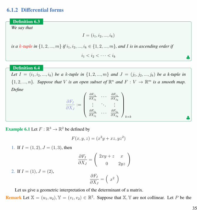
6.1.2 Differential forms
Definition 6.3
♣
We say thatI = (i1, i2, ..., ik)
is a k-tuple in 1, 2, ...,m if i1, i2, ..., ik ∈ 1, 2, ...,m, and I is in ascending order if
i1 < i2 < · · · < ik
Definition 6.4
♣
Let I = (i1, i2, ..., ik) be a k-tuple in 1, 2, ...,m and J = (j1, j2, ..., jk) be a k-tuple in1, 2, ..., n. Suppose that V is an open subset of Rn and F : V → Rm is a smooth map.Define
∂FI∂XJ
:=
∂Fi1
∂Xj1· · · ∂Fi1
∂Xjk... . . . ...∂Fik
∂Xj1· · · ∂Fik
∂Xjk
k×k
Example 6.1 Let F : R3 → R2 be defined by
F (x, y, z) = (x2y + xz, yz2)
1. If I = (1, 2), J = (1, 3), then
∂FI∂XJ
=
(2xy + z x
0 2yz
)2. If I = (1), J = (2),
∂FI∂XJ
=(x2)
Let us give a geometric interpretation of the determinant of a matrix.Remark Let X = (u1, u2),Y = (v1, v2) ∈ R2. Suppose that X,Y are not collinear. Let P be the
35

parallelogram determined by X and Y. We know that
area of P = ||X||||Y|| sin θ
where θ is the angle between X and Y determined by the formula
cos θ =X · Y||X||||Y||
Note that
sin θ =√1− cos2 θ =
√1− (
X · Y||X||||Y||
)2 =1
||X||||Y||√(||X||||Y||)2 − (X · Y)2
The area of P is
||X||||Y|| sin θ =√(u21 + u22)(v
21 + v22)− (u1v1 + u2v2)2
=√u21v
22 + u22v
21 − 2u1v1u2v2
=√
(u1v2 − u2v1)2
= | det
(u1 u2
v1 v2
)|
If there exists a linear transformation LA : R2 → R2 where A ∈ GL(2,R) with det(A) > 0 suchthat
LA(X) = e1, LA(Y) = e2
where e1, e2 is the standard ordered basis of R2, then
det
(u1 u2
v1 v2
)is positive. In this case, we say that the ordered basis X,Y and e1, e2 have the same orientation.
Let us look at integration from another viewpoint.Example 6.2
1. Let ϕ : [a, b]→ [a, b] be the identity function
ϕ(x) := x
36

and f : [a, b] → R be a smooth function. We consider fdx as a tool that can measure howlong is the length of ϕ. Write
(fdx)(ϕ) :=
∫[a,b]
f(ϕ(x))dϕ
dxdx =
∫ b
a
f(x)dx
2. Let ψ : [a, b]× [c, d]→ [a, b]× [c, d] be the identity map
ψ(x1, x2) := (x1, x2) = (ψ1(x1, x2), ψ2(x1, x2))
For any smooth function g : [a, b]× [c, d]→ R, we consider gdxdy as a tool that can measurehow large is the area of ψ. Write
(gdxdy)(ψ) =
∫[a,b]×[c,d]
g(ψ(x1, x2)) det∂ψ1,2
∂x1,2dV
=
∫[a,b]×[c,d]
g(x1, x2) det
(1 0
0 1
)dV
=
∫[a,b]×[c,d]
gdV
Definition 6.5
♣
Let V ⊂ Rn be an open set and k ∈ N. A simple k-form on V is a linear functionfdXI : Ck(V )→ R defined by
(fdXI)(φ) :=
∫[0,1]k
f(φ(u)) det∂φI
∂u1,...,kdV
=
∫ 1
0
· · ·∫ 1
0
f(φ(u)) det(∂φI
∂u1,...,k)du1...duk
where I is a k-tuple in 1, ..., n, f : V → R is a smooth function and φ is a k-cell in V . IfI = (i1, i2, ..., ik), we also write
dXI = dxi1dxi2 · · · dxik
Example 6.3 Let φ : [0, 1]2 → R3 be defined by
φ(u1, u2) = (2u1 + 3u2, u1, u2)
37

Then φ is 2-cell for R3. Let I = (1, 2). Then
∂φI∂u1,2
=
(2 3
1 0
)and
(dXI)(φ) =
∫[0,1]2
det∂φI∂u1,2
dV =
∫ 1
0
∫ 1
0
(−3)du1du2 = −3
Proposition 6.1
♠
Let I = (i1, i2, ..., ik) where k ∈ N. If π : 1, 2, ..., k → 1, 2, ..., k is a permutation and
πI = (iπ(1), iπ(2), ..., iπ(k))
thendXπI = sgn(π)dXI
Proof Let φ be a k-cell. Then
(dXπI)(φ) =
∫[0,1]k
det∂φπI∂u1,...,,k
dV =
∫[0,1]k
sgn(π) det∂φI
∂u1,...,kdV = sgn(π)(dXI)(φ)
HencedXπI = sgn(π)dXI
Example 6.4 On R4, we have1.
dxdy = −dydx
2.dxdydzdw = −dxdwdzdy
in which we may consider I = (1, 2, 3, 4) and πI = (1, 4, 3, 2).
38

Example 6.5 Let φ : [0, 1]5 → R6 be defined by
φ(u1, u2, u3, u4, u5) = (2u1, 3u2, 4u3, 5u4 + 6u5, u1 + u2, u1 + u3)
Let I = (1, 2, 3, 4, 5) and
π =
(1 2 3 4 5
4 3 1 5 2
)=(
1 4 5 2 3)= (13)(12)(15)(14)
Then πI = (4, 3, 1, 5, 2), sgn(π) = 1, and
φπI(u1, u2, u3, u4, u5) = (5u4 + 6u5, 4u3, 2u1, u1 + u2, 3u2, u1 + u3)
∂φπI∂u1,..,5
=
0 0 0 5 6
0 0 4 0 0
2 0 0 0 0
1 1 0 0 0
0 3 0 0 0
and
∂φI∂u1,..,5
=
2 0 0 0 0
0 3 0 0 0
0 0 4 0 0
0 0 0 5 6
1 1 0 0 0
Therefore ∂ϕπI
∂u1,...,5is obtained from ∂ϕI
∂u1,...,5by exchanging rows 4 times. Hence
det∂φπI∂u1,...,5
= det∂φI
∂u1,...,5
39

Corollary 6.1
If I = (i1, ..., ik) and ij1 = ij2 for some j1 = j2, then
dXI = 0
Proof Let π be the k-permutation that interchanges j1 and j2 only. Since sgn(π) = −1,
dXπI = −dXI
From ij1 = ij2 , we havedXπI = dXI
This implies dXI = −dXI and 2dXI = 0 which gives us
dXI = 0
Example 6.6 In any open set V ⊂ Rn, we always have1.
dxdx = 0
2.dxdydzdy = 0
Definition 6.6
♣
Let V be an open subset of Rn. A 0-form on V is a smooth function f : V → R. For k ∈ N, ak-form on V is a finite sum of simple k-forms on V . More explicitly, a k-form on V is a linearfunction
∑I
fIdXI : Ck(V )→ R defined by
(∑I
fIdXI)(ϕ) :=∑I
(fIdXI)(ϕ)
where ϕ is a k-chain on V and the sum is a finite sum. We denote by Ωk(V ) the set of allk-forms on V .
40

Example 6.71. For f, g : R2 → R smooth functions,
f(x, y)dx+ g(x, y)dy
is an 1-form on R2.2. For h : R2 → R,
h(x, y)dxdy
is a 2-form on R2.Remark Note that I0 := 1. If φ : I0 → V is a 0-cell and f : V → R is a 0-form, then
(f)(φ) := f(φ(1))
If∑m
i=1 aiφi is a 0-chain in V , then
(f)(m∑i=1
aiφi) =m∑i=1
aif(φi(1))
Corollary 6.2
If V is open in Rn and k > n, thenΩk(V ) = 0
Proof Let I = (i1, i2, ..., ik) be a k-tuple in 1, 2, ..., n. Since k > n, ij1 = ij2 for some j1 = j2.Then by Corollary 6.1, dXI = 0. Hence
Ωk(V ) = 0
Example 6.8Ω4(R3) = 0
41

Remark LetI +k = I|I is an ascending k-tuple in 1, 2, ..., n
Note thatdXI |I ∈ I +
k
is a basis forΩk(V ) over C ∞(V ). In the language of algebra, Ωk(V ) is the C ∞(V )-module generatedby
dXI |I ∈ I +k
42

K Exercise 6.1 k
1. For i = 1, 2, 3, let ϕi : [0, 1]2 → R be defined by
ϕi(x1, x2) := 3x1 + 4ix2 + i
and ϕ, ψ : [0, 1]2 → R3 be the smooth functions defined by
ϕ(x1, x2) := (ϕ1(x1, x2), ϕ2(x1, x2), ϕ3(x1, x2))
ψ(x1, x2) := (2, ϕ1(x1, x2) + ϕ2(x1, x2), ϕ3(x1, x2) + x21)
Finddx1dx3(2ϕ+ 3ψ)
where 2ϕ+ 3ψ is a 2-chain, not a function.2. Let ϕ : In → Rn be defined by
ϕ(u1, ..., un) = (u1, ..., un)
and ω = dx1dx2 · · · dxn. Find ω(ϕ).3. (a). Suppose that
Xi :=3∑j=1
aijej
where i = 1, 2, 3 are 3 linearly independent vectors in R3. Let
P := aX1 + bX2 + cX3|0 ≤ a, b, c ≤ 1
be the parallelogram spanned by X1,X2,X3. Find the volume
V ol(P ) :=
∫P
χPdV
of P .(b). Let ϕ : [0, 1]3 → R3 be defined by
ϕ(u1, u2, u3) := u1X1 + u2X2 + u3X3
43

Finddx1dx2dx3(ϕ)
(c). Generalize above results to vectors in Rn.
44

6.2 Wedge product and the exterior derivative
6.2.1 Wedge product
Definition 6.7. Wedge product
♣
Suppose that V ⊂ Rn is an open subset. Let
α =∑I
aIdXI
be a k-form andβ =
∑J
bJdXJ
be an `-form on V , their wedge product is the (k + l)-form
α ∧ β =∑I,J
aIbJdXIJ
where I = (i1, i2, ..., ik), J = (j1, j2, ..., jl), IJ = (i1, i2, ..., ik, j1, j2, ..., jl).
Example 6.9 Letα = fdx+ gdy ∈ Ω1(R3)
β = pdxdz + qdydz = −pdzdx− qdzdy ∈ Ω2(R3)
Then
(fdx+ gdy) ∧ (pdxdz + qdydz) = fpdxdxdz + fqdxdydz + gpdydxdz + gqdydydz
= (fq − gp)dxdydz
and
(fdx+ gdy) ∧ (−pdzdx− qdzdy) = −fpdxdzdx− fqdxdzdy − gpdydzdx− gqdydzdy
= (fq − gp)dxdydz
45

Definition 6.8
♣
A k-permutation π : 1, ..., k → 1, ..., k and an `-permutation σ : 1, ..., ` → 1, ..., `induce a (k + `)-permutation
(π, σ) =
(1 · · · k k + 1 · · · k + `
π(1) · · · π(k) k + σ(1) · · · k + σ(`)
)
Remarksgn(π, σ) = sgn(π)sgn(σ)
Lemma 6.1
Suppose that I is a k-tuple, J is an `-tuple in 1, ..., n, and π, σ are k-permutation and`-permutation respectively. If I ′ = π(I), J ′ = σ(J), then
dXI′J ′ = sgn(π)sgn(σ)dXIJ
Proof Let I = (i1, ..., ik) and J = (j1, ..., jℓ). Write
J = (ik+1, ..., ik+ℓ)
Then
(π, σ)(IJ) = (iπ(1), ..., iπ(k), ik+σ(1), ..., ik+σ(ℓ))
= (iπ(1), ..., iπ(k), jσ(1), ..., jσ(ℓ))
= π(I)σ(J)
We have
dXI′J ′ = dXπ(I)σ(J) = dX(π,σ)(IJ) = sgn(π, σ)dXIJ = sgn(π)sgn(σ)dXIJ
Proposition 6.2
♠The wedge product is well-defined.
46

Proof Let V ⊂ Rn be an open subset. Suppose that
α =∑I
fIdXI =∑I′
f ′I′dXI′ ∈ Ωk(V )
β =∑J
gJdXJ =∑J ′
g′J ′dXJ ′ ∈ Ωℓ(V )
where all I ′, J ′ are in ascending order. We need to show that∑I,J
fIgJdXIJ =∑I′,J ′
f ′I′g
′J ′dXI′J ′
LetΓ(I ′) := I|π(I) = I ′ for some k-permutation π
Γ(J ′) := J |σ(J) = J ′ for some `-permuation σ
andπ(I, I ′) := the k-permuation that maps I to I ′
σ(J, J ′) := the `-permuation that maps J to J ′
Thenf ′I′ =
∑I∈Γ(I′)
fIsgn(π(I, I ′))
g′J ′ =∑
J∈Γ(J ′)
gIsgn(σ(J, J ′))
47

Then ∑I′,J ′
f ′I′g
′J ′dXI′J ′ =
∑I′,J ′
∑I∈Γ(I′)
fIsgn(π(I, I ′))∑
J∈Γ(J ′)
gJsgn(σ(J, J ′))dXI′J ′
=∑I′,J ′
∑I∈Γ(I′)
∑J∈Γ(J ′)
fIgJsgn(π(I, I ′))sgn(σ(J, J ′))dXI′J ′
=∑I′,J ′
∑I∈Γ(I′)
∑J∈Γ(J ′)
fIgJdXIJ
=∑I,J
fIgJdXIJ
Proposition 6.3
♠
Let V be an open subset of Rn and Ω•(V ) :=⊕∞
k=0 Ωk(V ). The wedge product
∧ : Ω•(V )× Ω•(V )→ Ω•(V )
satisfies:(i) distributivity:
(α + β) ∧ γ = α ∧ γ + β ∧ γ
(ii) associativity:(α ∧ β) ∧ γ = α ∧ (β ∧ γ)
(iii) graded-commutativity: For α ∈ Ωk(V ), β ∈ Ωl(V )
α ∧ β = (−1)klβ ∧ α
Proof(i) For α, β, γ ∈ Ω•(V ), by setting some coefficients to be 0, we may use same indexes to write
α =∑I
aIdXI , β =∑I
bIdXI
48

Let γ =∑
J cJdXJ . Then
(α + β) ∧ γ = (∑I
(aI + bI)dXI) ∧ (∑J
cJdXJ)
=∑I,J
(aI + bI)cJdXIJ
=∑I,J
aIcJdXIJ +∑I,J
bIcJdXIJ
= α ∧ γ + β ∧ γ
(ii) Let α =∑
I aIdXI , β =∑
J bJdXJ and γ =∑
L cLdXL be some differential forms on V .Then
(α ∧ β) ∧ γ = (∑I,J
aIbJdXIJ) ∧∑L
cLdXL
=∑I,J,L
(aIbJ)cLdX(IJ)L
=∑I,J,L
aI(bJcL)dXI(JL)
= (∑I
aIdXI)(∑J,L
bJcLdXJL)
= α ∧ (β ∧ γ)
(iii) Let α =∑
I aIdXI ∈ Ωk(V ) and β =∑
J bJdXJ ∈ Ωl(V ). For
I = (i1, · · · , ik), J = (j1, · · · , jl)
IJ = (i1, · · · , ik, j1, · · · , jl), JI = (j1, · · · , jl, i1, · · · , ik)
To get dXJdXis from dXisdXJ , each is needs to exchange its position with j1, · · · , jl, henceproduces a (−1)l. The total number of exchanges needed to get dXJI from dXIJ is kl, hence
α ∧ β =∑I,J
aIbJdXIJ = (−1)kl∑J,I
bJaIdXJI = (−1)klβ ∧ α
49
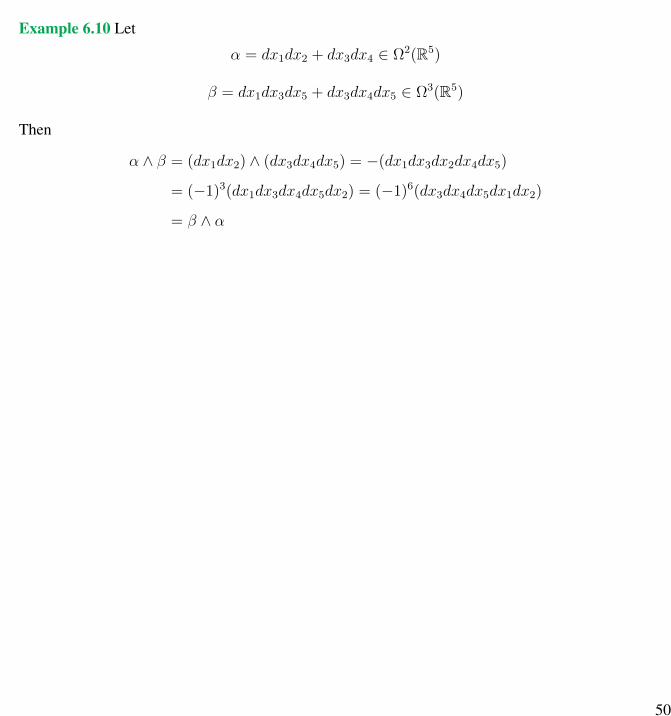
Example 6.10 Letα = dx1dx2 + dx3dx4 ∈ Ω2(R5)
β = dx1dx3dx5 + dx3dx4dx5 ∈ Ω3(R5)
Then
α ∧ β = (dx1dx2) ∧ (dx3dx4dx5) = −(dx1dx3dx2dx4dx5)
= (−1)3(dx1dx3dx4dx5dx2) = (−1)6(dx3dx4dx5dx1dx2)
= β ∧ α
50
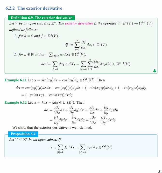
6.2.2 The exterior derivative
Definition 6.9. The exterior derivative
♣
Let V be an open subset of Rn. The exterior derivative is the operator d : Ωk(V )→ Ωk+1(V )
defined as follows:1. for k = 0 and f ∈ Ω0(V ),
df :=n∑i=1
∂f
∂xidxi ∈ Ω1(V )
2. for k ∈ N and α =∑
|I|=k aIdXI ∈ Ωk(V ),
dα :=∑|I|=k
daI ∧ dXI =∑|I|=k
n∑i=1
∂aI∂xi
dxidXI ∈ Ωk+1(V )
Example 6.11 Let α = sin(xy)dx+ cos(xy)dy ∈ Ω1(R2). Then
dα = cos(xy)(y)dxdx+ cos(xy)(x)dydx+ (−sin(xy)y)dxdy + (−sin(xy)x)dydy
= (−ysin(xy)− xcos(xy))dxdy
Example 6.12 Let α = fdx+ gdy ∈ Ω1(R2). Then
dα = (∂f
∂xdx+
∂f
∂ydy)dx+ (
∂g
∂xdx+
∂g
∂ydy)dy
=∂f
∂ydydx+
∂g
∂xdxdy = (
∂g
∂x− ∂f
∂y)dxdy
We show that the exterior derivative is well-defined.
Proposition 6.4Let V ⊂ Rn be an open subset. If
α =∑|I|=k
fIdXI =∑|J |=k
gJdXJ ∈ Ωk(V )
51

♠
thend(∑|I|=k
fIdXI) = d(∑|J |=k
gJdXJ)
Proof Since the differential of a smooth function is unique, there is nothing to prove for k = 0. Letk ∈ N. Write
α =∑I′
f ′I′dXI′
where every I ′ is a k-tuple in ascending order. We use notations as in the proof of Proposition 6.2.Note that
f ′I′ =
∑I∈Γ(I′)
fIsgn(π(I, I ′))
anddf ′I′ =
∑I∈Γ(I′)
dfIsgn(π(I, I ′))
Then
d(∑I′
f ′I′dXI′) =
∑I′
df ′I′ ∧ dXI′
=∑I′
∑I∈Γ(I′)
dfIsgn(π(I, I ′)) ∧ dXI′
=∑I′
∑I∈Γ(I′)
dfI ∧ dXI
=∑I
dfI ∧ dXI
= d(∑I
fIdXI)
This proves that d is well-defined.
52

Proposition 6.5
♠
Let V be an open subset ofRn and k ∈ N∪0. The exterior derivative d : Ωk(V )→ Ωk+1(V )
satisfies:
(i)d(aα + bβ) = adα + bdβ
for all a, b ∈ R, α, β ∈ Ωk(V ).(ii) If α ∈ Ωk(V ), β ∈ Ωl(V ), then
d(α ∧ β) = dα ∧ β + (−1)kα ∧ dβ
(iii)d2 = 0
That meansd(dα) = 0
for all α ∈ Ωk(V )
Proof(i) For f, g ∈ Ω0(V ),
d(af + bg) =n∑i=1
∂(af + bg)
∂xidxi =
n∑i=1
(a∂f
∂xi+ b
∂g
∂xi)dxi
= a
n∑i=1
∂f
∂xidxi + b
n∑i=1
∂g
∂xidxi
= adf + bdg
53
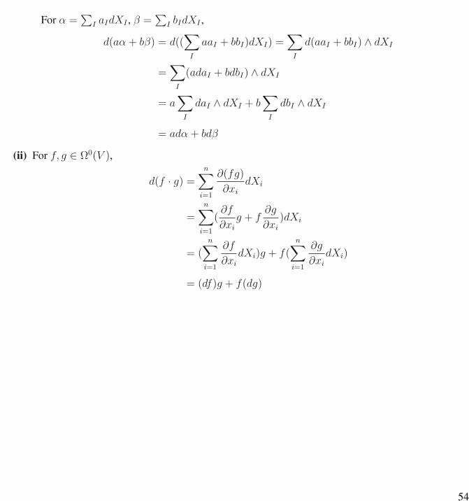
For α =∑
I aIdXI , β =∑
I bIdXI ,
d(aα + bβ) = d((∑I
aaI + bbI)dXI) =∑I
d(aaI + bbI) ∧ dXI
=∑I
(adaI + bdbI) ∧ dXI
= a∑I
daI ∧ dXI + b∑I
dbI ∧ dXI
= adα + bdβ
(ii) For f, g ∈ Ω0(V ),
d(f · g) =n∑i=1
∂(fg)
∂xidXi
=n∑i=1
(∂f
∂xig + f
∂g
∂xi)dXi
= (n∑i=1
∂f
∂xidXi)g + f(
n∑i=1
∂g
∂xidXi)
= (df)g + f(dg)
54

For α =∑
I aIdXI , β =∑
J bJdXJ ,
d(α ∧ β) = d(∑I,J
aIbJdXIJ) =∑I,J
d(aIbJ) ∧ dXIJ
=∑I,J
((daI)bJ + aI(dbJ)) ∧ dXIJ
=∑I,J
(daI)bJ ∧ dXI ∧ dXJ +∑I,J
aI(dbJ) ∧ dXI ∧ dXJ
= (∑I
daIdXI) ∧ (∑J
bJdXJ) +∑I,J
aI(dbJ) ∧ dXI ∧ dXJ
= dα ∧ β +∑I,J
aI
n∑i=1
∂bJ∂xi
dxi ∧ dXI ∧ dXJ
= dα ∧ β +∑I
aI(−1)kdXI ∧∑J
(n∑i=1
∂bJ∂xi
dxi) ∧ dXJ
= dα ∧ β + (−1)kα ∧ dβ
(iii) For f ∈ Ω0(V ), df =∑n
i=1∂f∂xidxi
d2f =n∑i=1
n∑j=1
∂2f
∂xj∂xidxjdxi
Note that∂2f
∂xj∂xidxjdxi = −
∂2f
∂xi∂xjdxidxj
55

Hence,
d2f =∑i<j
∂2f
∂xj∂xidxjdxi +
∑i=j
∂2f
∂xj∂xidxjdxi +
∑i>j
∂2f
∂xj∂xidxjdxi
=∑i<j
∂2f
∂xj∂xidxjdxi +
∑i>j
∂2f
∂xj∂xidxjdxi
=∑i<j
∂2f
∂xj∂xidxjdxi −
∑i>j
∂2f
∂xi∂xjdxidxj
=∑i<j
∂2f
∂xj∂xidxjdxi −
∑i<j
∂2f
∂xj∂xidxjdxi
= 0
Note thatd2XI = d(1dXI) = 0
For α =∑
|I|=k aIdXI ∈ Ωk(V ),
d2α = d(dα) = d(∑|I|=k
daI ∧ dXI) =∑|I|=k
(d2aI ∧ dXI − daI ∧ d2XI) = 0
Example 6.13 Let ω = sin(xy)dx+ zcosydy + xdz ∈ Ω1(R3). Then
dω = cos(xy)xdydx+ cosydzdy + dxdz
andd2ω = 0 + 0 + 0 = 0
56

K Exercise 6.2 k
1. Suppose that V is an open set of Rn. Let ϕ ∈ Ωk(V ) where k is an odd integer. Show thatϕ ∧ ϕ = 0.
2. Let
ϕ = xdx− ydy
ψ = zdxdy + xdydz
θ = zdy
Compute ϕ ∧ ψ, θ ∧ ϕ ∧ ψ, dϕ, dψ, dθ.3. Let
ω = dx1dx2 + dx3dx4 + · · ·+ dx2n−1dx2n ∈ Ω2(R2n)
Compute ωn the wedge product of n copies of ω.4. A function f : R3 → R is said to be homogeneous of degree k if
f(tx, ty, tz) = tkf(x, y, z)
for t > 0, (x, y, z) ∈ R3. Show that(a). If f is smooth and homogeneous of degree k, then
x∂f
∂x+ y
∂f
∂y+ z
∂f
∂z= kf
(b). If ω = adx+ bdy+ cdz ∈ Ω1(R3), a, b, c are homogeneous of degree k and dω = 0, finda smooth function g such that ω = dg.
(c). If α = adydz + bdzdx+ cdxdy where a, b, c are homogeneous of degree k and dα = 0,find β ∈ Ω1(R3) such that α = dβ.
57

6.3 Pushforward and pullback
Definition 6.10. Pushforward and pullback
♣
Let V be an open subset of Rn, W be an open subset of Rm, and F : V → W be a smoothmap. If ϕ is a k-cell in V , define
F∗ϕ = F ϕ
Then F∗ϕ is a k-cell in W . Extending by linearity, we get a map F∗ : Ck(V )→ Ck(W ) by
F∗(l∑
i=1
aiϕi) :=l∑
i=1
aiF∗ϕi
The map F∗ is called the pushforward induced by F . Furthermore, F also induces a linearmap F ∗ : Ωk(W )→ Ωk(V ) by
(F ∗ω)(ϕ) := ω(F∗ϕ)
where ϕ ∈ Ck(V ) and ω ∈ Ωk(W ). The map F ∗ is called the pullback induced by F .
Example 6.14 Let V = BR2
1 (0) ⊂ R2, W = BR3
1 (0) ⊂ R3,
F (x, y) = (x2, y4,√2xy2)
Note that if (x, y) ∈ V , then
(x2)2 + (y4)2 + (√2xy2)2 = x4 + y8 + 2x2y4 = (x2 + y4)2 ≤ (x2 + y2)2 < 1
hence F is a function from V to W . Given ϕ : [0, 1]→ V where
ϕ(t) = (1
2t,1
3t)
Then(F∗ϕ)(t) = F (ϕ(t)) = F (
1
2t,1
3t) = (
1
4t2,
1
81t4,
√2
18t3)
Letω = xyzdx+ x2dy + ydz ∈ Ω1(W )
58

Then
(F ∗ω)(ϕ) = ω(F∗ϕ) = ω(F ϕ)
=
∫ 1
0
(1
4t2)(
1
81t4)(
√2
18t3)(
1
2t) + (
1
4t2)2(
4
81t3) + (
1
81t4)(
√2
6t2)dt
=
√2
8 · 81 · 181
11+
1
4 · 811
8+
√2
6 · 811
7
Definition 6.11
♣
Let k ∈ N and k ≤ n. Suppose that A is a k × n matrix and B is an n × k matrix. ForJ = (j1 < j2 < · · · < jk) an ascending k-tuple in 1, ..., n, denote by
AJ :=
| | · · · |cj1 cj2 · · · cjk
| | · · · |
the k × k-matrix formed by the j1-th, j2-th,..., jk-th columns of A, and denote by
BJ :=
− rj1 −− rj2 −...
......
− rjk −
the k × k-matrix formed by the j1-th, j2-th,...,jk-th rows of B.
The following result from linear algebra will be needed in the proof of the next theorem.
Theorem 6.1. The Cauchy-Binet formula
Let k ∈ N and k ≤ n. Suppose that A is a k × n matrix and B is an n× k matrix then
det(AB) =∑
J ascending k-tuplein 1, ..., n
(detAJ)(detBJ)
59
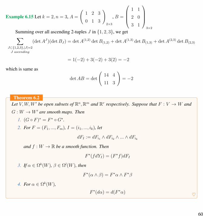
Example 6.15 Let k = 2, n = 3, A =
(1 2 3
0 1 3
)2×3
, B =
1 1
2 0
3 1
3×2
Summing over all ascending 2-tuples J in 1, 2, 3, we get∑J⊂1,2,3,|J |=2
J ascending
(detAJ)(detBJ) = detA(1,2) detB(1,2) + detA(1,3) detB(1,3) + detA(2,3) detB(2,3)
= 1(−2) + 3(−2) + 3(2) = −2
which is same as
detAB = det
(14 4
11 3
)= −2
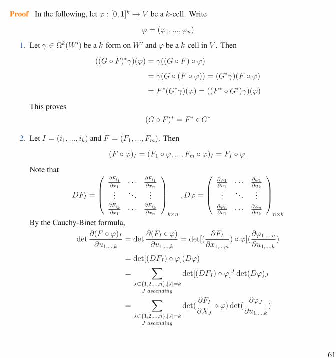
Theorem 6.2
Let V,W,W ′ be open subsets of Rn,Rm and Rr respectively. Suppose that F : V → W andG : W → W ′ are smooth maps. Then
1. (G F )∗ = F ∗ G∗.2. For F = (F1, ..., Fm), I = (i1, ..., ik), let
dFI := dFi1 ∧ dFi2 ∧ ... ∧ dFikand f : W → R be a smooth function. Then
F ∗(fdYI) = (F ∗f)dFI
3. If α ∈ Ωk(W ), β ∈ Ωl(W ), then
F ∗(α ∧ β) = F ∗α ∧ F ∗β
4. For α ∈ Ωk(W ),F ∗(dα) = d(F ∗α)
60
Proof In the following, let ϕ : [0, 1]k → V be a k-cell. Write
ϕ = (ϕ1, ..., ϕn)
1. Let γ ∈ Ωk(W ′) be a k-form on W ′ and ϕ be a k-cell in V . Then
((G F )∗γ)(ϕ) = γ((G F ) ϕ)
= γ(G (F ϕ)) = (G∗γ)(F ϕ)
= F ∗(G∗γ)(ϕ) = ((F ∗ G∗)γ)(ϕ)
This proves(G F )∗ = F ∗ G∗
2. Let I = (i1, ..., ik) and F = (F1, ..., Fm). Then
(F ϕ)I = (F1 ϕ, ..., Fm ϕ)I = FI ϕ.
Note that
DFI =
∂Fi1
∂x1· · · ∂Fi1
∂xn... . . . ...
∂Fik
∂x1· · · ∂Fik
∂xn
k×n
, Dϕ =
∂φ1
∂u1· · · ∂φ1
∂uk... . . . ...∂φn
∂u1· · · ∂φn
∂uk
n×k
By the Cauchy-Binet formula,
det∂(F ϕ)I∂u1,...,k
= det∂(FI ϕ)∂u1,...,k
= det[(∂FI
∂x1,...,n) ϕ](∂ϕ1,...,n
∂u1,...,k)
= det[(DFI) ϕ](Dϕ)
=∑
J⊂1,2,...,n,|J |=kJ ascending
det[(DFI) ϕ]J det(Dϕ)J
=∑
J⊂1,2,...,n,|J |=kJ ascending
det(∂FI∂XJ
ϕ) det( ∂ϕJ∂u1,...,k
)
61
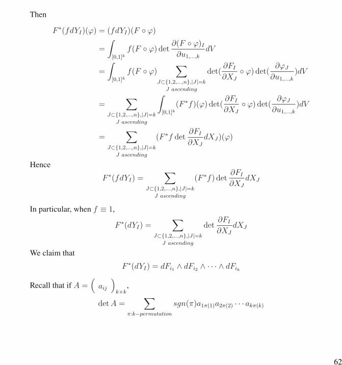
Then
F ∗(fdYI)(ϕ) = (fdYI)(F ϕ)
=
∫[0,1]k
f(F ϕ) det ∂(F ϕ)I∂u1,...,k
dV
=
∫[0,1]k
f(F ϕ)∑
J⊂1,2,...,n,|J |=kJ ascending
det(∂FI∂XJ
ϕ) det( ∂ϕJ∂u1,...,k
)dV
=∑
J⊂1,2,...,n,|J |=kJ ascending
∫[0,1]k
(F ∗f)(ϕ) det(∂FI∂XJ
ϕ) det( ∂ϕJ∂u1,...,k
)dV
=∑
J⊂1,2,...,n,|J |=kJ ascending
(F ∗f det∂FI∂XJ
dXJ)(ϕ)
HenceF ∗(fdYI) =
∑J⊂1,2,...,n,|J |=k
J ascending
(F ∗f) det∂FI∂XJ
dXJ
In particular, when f ≡ 1,
F ∗(dYI) =∑
J⊂1,2,...,n,|J |=kJ ascending
det∂FI∂XJ
dXJ
We claim thatF ∗(dYI) = dFi1 ∧ dFi2 ∧ · · · ∧ dFik
Recall that if A =(aij
)k×k
,
detA =∑
π:k−permutation
sgn(π)a1π(1)a2π(2) · · · akπ(k)
62
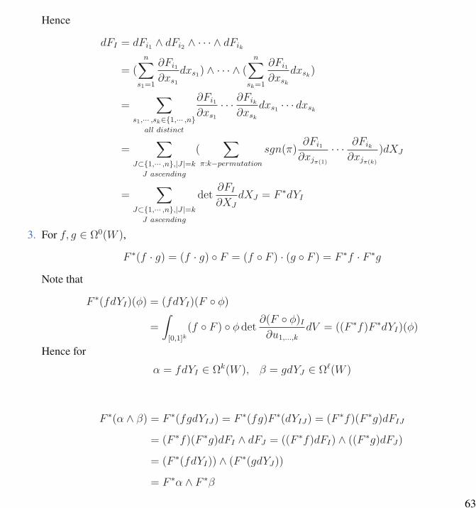
Hence
dFI = dFi1 ∧ dFi2 ∧ · · · ∧ dFik
= (n∑
s1=1
∂Fi1∂xs1
dxs1) ∧ · · · ∧ (n∑
sk=1
∂Fi1∂xsk
dxsk)
=∑
s1,··· ,sk∈1,··· ,nall distinct
∂Fi1∂xs1
· · · ∂Fik∂xsk
dxs1 · · · dxsk
=∑
J⊂1,··· ,n,|J |=kJ ascending
(∑
π:k−permutation
sgn(π)∂Fi1∂xjπ(1)
· · · ∂Fik∂xjπ(k)
)dXJ
=∑
J⊂1,··· ,n,|J |=kJ ascending
det∂FI∂XJ
dXJ = F ∗dYI
3. For f, g ∈ Ω0(W ),
F ∗(f · g) = (f · g) F = (f F ) · (g F ) = F ∗f · F ∗g
Note that
F ∗(fdYI)(φ) = (fdYI)(F φ)
=
∫[0,1]k
(f F ) φ det ∂(F φ)I∂u1,...,k
dV = ((F ∗f)F ∗dYI)(φ)
Hence forα = fdYI ∈ Ωk(W ), β = gdYJ ∈ Ωℓ(W )
F ∗(α ∧ β) = F ∗(fgdYIJ) = F ∗(fg)F ∗(dYIJ) = (F ∗f)(F ∗g)dFIJ
= (F ∗f)(F ∗g)dFI ∧ dFJ = ((F ∗f)dFI) ∧ ((F ∗g)dFJ)
= (F ∗(fdYI)) ∧ (F ∗(gdYJ))
= F ∗α ∧ F ∗β
63

Since F ∗ is linear, the result is true for all k, `-forms on W .4. Let f ∈ Ω0(W ). We have
F ∗(df) = F ∗(m∑i=1
∂f
∂yidyi) =
m∑i=1
F ∗(∂f
∂yi)F ∗dyi
=m∑i=1
∂f
∂yi FdFi =
m∑i=1
∂f
∂yi F (
n∑j=1
∂Fi∂xj
dxj)
=n∑j=1
(m∑i=1
∂f
∂yi F )(∂Fi
∂xj))dxj =
n∑j=1
∂(f F )∂xj
dxj
= d(f F ) = d(F ∗f)
For ω = fdYI ,
F ∗(dω) = F ∗(df ∧ dYI) = F ∗(df) ∧ F ∗(dYI)
= d(F ∗f) ∧ dFI = d(F ∗f) ∧ dFI + F ∗f ∧ d(dFI)
= d((F ∗f) ∧ dFI) = d((F ∗f) ∧ (F ∗dYI))
= dF ∗(fdYI) = d(F ∗ω).
64

K Exercise 6.3 k
1.
65

6.4 Stokes’ theorem
Definition 6.12
♣
Let V be an open subset of Rn and w ∈ Ωk(V ). If φ is a k−cell in V , denote∫ϕ
ω := ω(φ)
If Φ =∑N
j=1 ajφj ∈ Ck(V ), denote ∫Φ
ω :=N∑j=1
ai
∫ϕj
ω
Definition 6.13
♣
Let V ⊂ Rn be an open subset. Denote
C−1(V ) := 0
For k = 0, defineτ 1,00 , τ 1,10 : [0, 1]0 := 1 → [0, 1]
byτ 1,00 (1) := 0, τ 1,10 (1) := 1
For k ∈ N and 1 ≤ j ≤ k + 1, define τ j,1k , τ j,0k : [0, 1]k → [0, 1]k+1 byτ j,0k (u1, · · · , uk) = (u1, · · · , uj−1, 0, uj, · · · , uk)τ j,1k (u1, · · · , uk) = (u1, · · · , uj−1, 1, uj, · · · , uk)
66
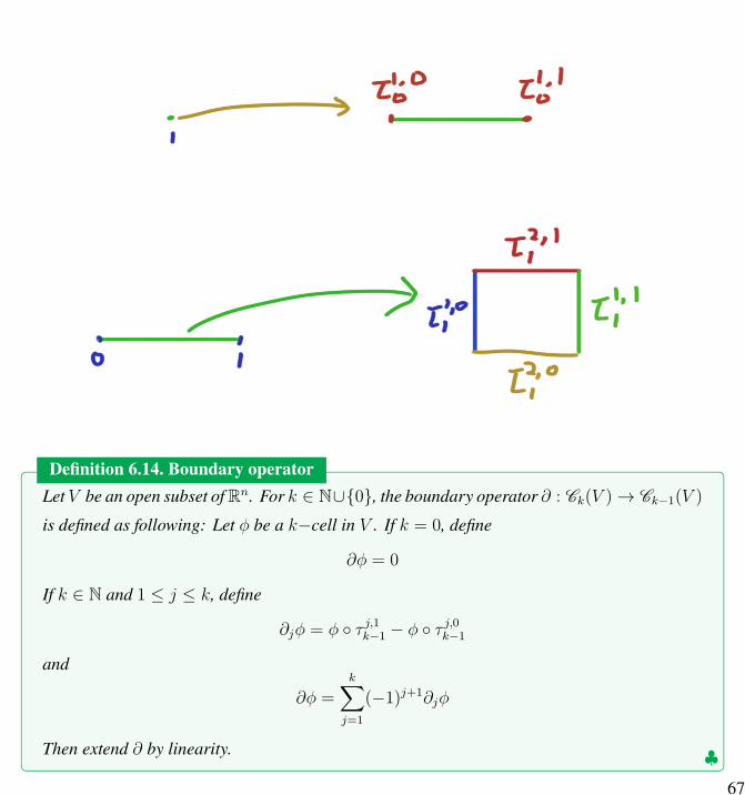
Definition 6.14. Boundary operator
♣
Let V be an open subset ofRn. For k ∈ N∪0, the boundary operator ∂ : Ck(V )→ Ck−1(V )
is defined as following: Let φ be a k−cell in V . If k = 0, define
∂φ = 0
If k ∈ N and 1 ≤ j ≤ k, define
∂jφ = φ τ j,1k−1 − φ τj,0k−1
and
∂φ =k∑j=1
(−1)j+1∂jφ
Then extend ∂ by linearity.
67

Example 6.16 Let φ : [0, 1]2 → R3 be defined by
φ(s, t) = (st, 3s+ t, s2 + t3)
Then
φ τ 1,11 (t) = φ(1, t) = (t, 3 + t, 1 + t3),
φ τ 1,01 (t) = φ(0, t) = (0, 0 + t, t3),
φ τ 2,11 (t) = φ(t, 1) = (t, 3t+ 1, t2 + 1),
φ τ 2,01 (t) = φ(t, 0) = (0, t, t2),
∂φ = ∂1φ− ∂2φ = (φ τ 1,11 − φ τ1,01 )− (φ τ 2,11 − φ τ
2,01 )
Example 6.17 Note that the boundary of a cell is a chain. The boundary of an 1-cell is a 0-chain.For example, let ϕ : [0, 1]→ R2 be defined by
ϕ(t) = (t, t2)
Then∂ϕ = ϕ(1)− ϕ(0) = (1, 1)− (0, 0)
where we identify (1, 1), (0, 0) with the functions from [0, 1]0 = 1 to R2 that map 1 to (1, 1), 0 to(0, 0) respectively. Hence (1, 1)− (0, 0) is a 0-chain not equal to (1, 1).
Lemma 6.2
Let W ⊂ Rn be an open set such that [0, 1]n ⊂ W . If ω ∈ Ωn−1(W ) and η : [0, 1]n → W isthe identity-inclusion n-cell in W , i.e.,
η(u1, ..., un) := (u1, ..., un)
then ∫η
dω =
∫∂η
ω
68

Proof Let
ω =n∑i=1
fidx1 ∧ ... ∧ dxi ∧ ... ∧ dxn
wheredx1 ∧ ... ∧ dxi ∧ ... ∧ dxn = dx1 ∧ ... ∧ dxi−1 ∧ dxi+1 ∧ ... ∧ dxn
and each fi : Rn → R is a smooth function. Then
dω =n∑i=1
(n∑j=1
∂fi∂xj
dxj)dx1 ∧ ... ∧ dxi ∧ ... ∧ dxn
=n∑i=1
∂fi∂xi
dxi ∧ dx1 ∧ ... ∧ dxi ∧ ... ∧ dxn
=n∑i=1
(−1)i−1 ∂fi∂xi
dx1 ∧ ... ∧ dxn
Note that∂η
∂u1,...,n= In = the n× n identity matrix
∫η
dω = (dω)(η) =n∑i=1
(−1)i−1
∫[0,1]n
∂fi∂xi
(η(u1, ..., un))(det∂η
∂u1,...,n)dVn
=n∑i=1
(−1)i−1
∫[0,1]n
∂fi∂xi
(u1, ..., un)dVn
Let Ij = (1, ..., j, ..., n). Then |Ij| = n− 1. Note that
τ i,0n−1(u) = (u1, ..., ui−1, 0, ui, ..., un−1)
τ i,1n−1(u) = (u1, ..., ui−1, 1, ui, ..., un−1)
and
det∂(τ i,0n−1)Ij∂u1,...,n−1
= det∂(τ i,1n−1)Ij∂u1,...,n−1
=
1 if i = j
0 otherwise
69
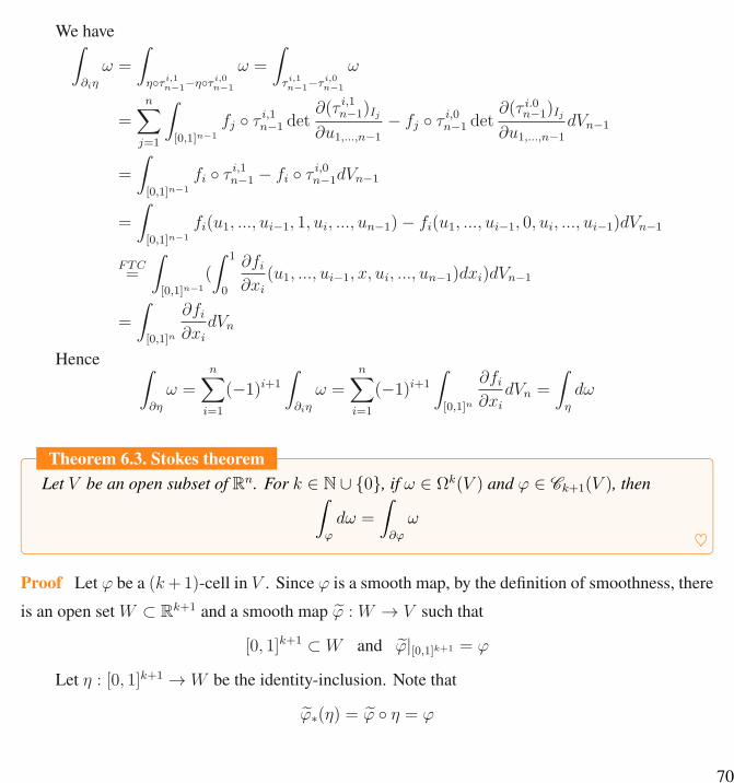
We have∫∂iη
ω =
∫ητ i,1n−1−ητ
i,0n−1
ω =
∫τ i,1n−1−τ
i,0n−1
ω
=n∑j=1
∫[0,1]n−1
fj τ i,1n−1 det∂(τ i,1n−1)Ij∂u1,...,n−1
− fj τ i,0n−1 det∂(τ i.0n−1)Ij∂u1,...,n−1
dVn−1
=
∫[0,1]n−1
fi τ i,1n−1 − fi τi,0n−1dVn−1
=
∫[0,1]n−1
fi(u1, ..., ui−1, 1, ui, ..., un−1)− fi(u1, ..., ui−1, 0, ui, ..., ui−1)dVn−1
FTC=
∫[0,1]n−1
(
∫ 1
0
∂fi∂xi
(u1, ..., ui−1, x, ui, ..., un−1)dxi)dVn−1
=
∫[0,1]n
∂fi∂xi
dVn
Hence ∫∂η
ω =n∑i=1
(−1)i+1
∫∂iη
ω =n∑i=1
(−1)i+1
∫[0,1]n
∂fi∂xi
dVn =
∫η
dω
Theorem 6.3. Stokes theorem
Let V be an open subset of Rn. For k ∈ N ∪ 0, if ω ∈ Ωk(V ) and ϕ ∈ Ck+1(V ), then∫φ
dω =
∫∂φ
ω
Proof Let ϕ be a (k+1)-cell in V . Since ϕ is a smooth map, by the definition of smoothness, thereis an open set W ⊂ Rk+1 and a smooth map ϕ : W → V such that
[0, 1]k+1 ⊂ W and ϕ|[0,1]k+1 = ϕ
Let η : [0, 1]k+1 → W be the identity-inclusion. Note that
ϕ∗(η) = ϕ η = ϕ
70

and
ϕ∗(∂η) = ϕ∗(k+1∑j=1
(−1)j+1∂jη)
=k+1∑j=1
(−1)j+1(ϕ (η τ j,1k )− ϕ (η τ j,0k ))
=k+1∑i=1
(−1)j+1(ϕ τ j,1k − ϕ τj,0k )
= ∂ϕ
Then ∫φ
dω =
∫φ∗(η)
dω = (dω)(ϕ∗η)
= (ϕ∗dω)(η) = (dϕ∗ω)(η) =
∫η
dϕ∗ω
=
∫∂η
ϕ∗ω = (ϕ∗ω)(∂η)
= ω(ϕ∗(∂η)) = ω(∂ϕ)
=
∫∂φ
ω
For a (k + 1)-chain ϕ =∑ℓ
i=1 aiϕi in V ,∫φ
dω =
∫∑ℓ
i=1 aiφi
dω =ℓ∑i=1
ai
∫φi
dω =ℓ∑i=1
ai
∫∂φi
ω =
∫∑ℓ
i=1 ai∂φi
ω =
∫∂φ
ω
This completes the proof.
71

K Exercise 6.4 k
1. In Rn, define∗(fdXI) = sgn(π)fdXJ
where |I| + |J | = n, I, J ascending, I ∪ J = 1, 2, ..., n and π is a n-permutation thatpermutes (1, 2, ..., n) to (IJ). For example in R3, ∗(dx2) = −dx1dx3. Extend by linearity weget a map
∗ : Ωk(Rn)→ Ωn−k(Rn)
which is called the Hodge star operator.(a). If ω = a12dx1 ∧ dx2 + a13dx1 ∧ dx3 + a23dx2 ∧ dx3 is a 2-form in R3, find ∗ω. If we
consider ω as a 2-form in R4, what is ∗ω? In general, if we consider ω as a 2-form in Rn,what is ∗ω?
(b). Show that ∗ ∗ ω = (−1)k(n−k)ω.(c). Find ∗d ∗ (dxI).(d). Let δ = (−1)n(k+1)+1 ∗ d∗ : Ωk(Rn) → Ωk−1(Rn) and ∆ = (dδ + δd) : Ωk(Rn) →
Ωk(Rn). Show that on 0-forms, ∆ = −∑n
j=1∂2
∂x2j.
(e). Let η : In → Rn be the inclusion map which we consider as a n-cell of Rn. Forα, β ∈ Ωk(Rn), define
< α, β >:=
∫η
α ∧ ∗β
Show that <,> is an inner product on Ωk(Rn).(f). Using Stokes’ theorem, show that δ is the adjoint of d, i.e., < dα, β >=< α, δβ > for
α or β having zero boundary values. (A form γ ∈ Ωk(V ) is said to have zero boundaryvalue if γ =
∑I aIdXI , then each aI(η τ j,i) = 0 for j = 1, ..., n, i = 0, 1.)
2. Show that ∂2c = 0 for c ∈ Ck(V ) where V is an open set of Rn.
72

6.5 Applications of the Stokes theorem
6.5.1 Reduction to some theorems in calculus
Definition 6.15
♣
A smooth map F : R3 → R3 is called a vector field on R3. Let
V F (R3) := F |F is a vector field on R3
For f : R3 → R a smooth function, define the gradient of f to be
∇(f) := (∂f
∂x,∂f
∂y,∂f
∂z)
For F = (F1, F2, F3) ∈ V F (R3), define the curl of F to be
curl(F ) := det
i j k∂∂x
∂∂y
∂∂z
F1 F2 F3
:= (∂F3
∂y− ∂F2
∂z, −(∂F3
∂x− ∂F1
∂z),∂F2
∂x− ∂F1
∂y)
and the divergence of F to be
div(F ) :=∂F1
∂x+∂F2
∂y+∂F3
∂z
Definition 6.16
♣
Suppose that we have homomorphisms between vector spaces
V1Ψ1 //
Φ1
V2
Φ2
W1
Ψ2 //W2
We say that the square is a commutative diagram if
Φ2 Ψ1 = Ψ2 Φ1
73

Proposition 6.6
♠
Each square in the following diagram is commutative:
0 //
Ω0(R3) d //
Φ0
Ω1(R3) d //
Φ1
Ω2(R3) d //
Φ2
Ω3(R3) d //
Φ3
0
0 / / C ∞(R3) ∇ // V F (R3)
curl // V F (R3)div // C ∞(R3) // 0
where those functions on the vertical arrows are defined as follow:
Φ0(f) := f
Φ1(f1dx+ f2dy + f3dz) := (f1, f2, f3)
Φ2(g1dxdy + g2dxdz + g3dydz) := (g3,−g2, g1)
Φ3(fdxdydz) = f
and they are isomorphisms between vector spaces.
Proof We prove that each square is commutative as follows:1.
Prove: Φ1 d = ∇ Φ0
For f ∈ Ω0(R3),
Φ1(df) = Φ1(∂f
∂xdx+
∂f
∂ydy +
∂f
∂zdz)
= (∂f
∂x,∂f
∂y,∂f
∂z)
= ∇(f) = ∇ Φ0(f)
2.Prove: Φ2 d = curl Φ1
74

Φ2 d(f1dx+ f2dy + f3dz)
= Φ2[∂f1∂y
dydx+∂f1∂z
dzdx+∂f2∂x
dxdy +∂f2∂z
dzdy +∂f3∂x
dxdz +∂f3∂y
dydz]
= Φ2[(∂f2∂x− ∂f1
∂y)dxdy + (
∂f3∂x− ∂f1
∂z)dxdz + (
∂f3∂y− ∂f2
∂z)dydz]
= ((∂f3∂y− ∂f2
∂z), −(∂f3
∂x− ∂f1
∂z), (
∂f2∂x− ∂f1
∂y))
= curl(f1, f2, f3) = curl(Φ1(f1dx+ f2dy + f3dz))
3.Prove: Φ3 d = div Φ2
Φ3d(g1dxdy + g2dxdz + g3dydz) = Φ3(∂g1∂z
dzdxdy +∂g2∂y
dydxdz +∂g3∂x
dxdydz)
= Φ3((∂g1∂z− ∂g2
∂y+∂g3∂x
)dxdydz)
=∂g1∂z− ∂g2
∂y+∂g3∂x
= div(g3,−g2, g1)
= div(Φ2(g1dxdy + g2dxdz + g3dydz))
Corollary 6.3
1.curl ∇ = 0
2.div curl = 0
Proof Recall that we have d2 = 0. Thus
75

1.curl ∇ = Φ2 d d Φ−1
0 = 0
2.div curl = Φ3 d d Φ−1
1 = 0
We leave the proof of the following result to the appendix of this section.
Theorem 6.4. Change of variables formula
Let U,W ⊂ Rn be some open sets and Φ : U → W be a C 1-diffeomorphism. Let f : W → Rbe a Riemann integrable function and R ⊂ U be a rectangle. Then∫
R
f Φ| det(DΦ)|dV =
∫Φ(R)
fdV
Definition 6.17
♣Let ϕ : [0, 1]k → Rn be a k-cell. We say that ϕ is injective if ϕ is an injective map.
We now use the language of forms and chains to interpret several results in calculus.
Definition 6.18
♣
Let C ∈ C1(R2). If there is an injective 2-cell ϕ : [0, 1]2 → R2 such that
∂ϕ = C and det(Dϕ) > 0
then we say that C is a positively oriented, piecewise-smooth, simple closed curve in the planeand D := image ϕ is the region bounded by C.
Remark We remark that even though we prove Stokes’ theorem for smooth forms and smooth chains,the proof goes through for C 1-forms and C 1-chains. We will use this C 1 version Stokes’ theorem inthe following paragraphs.
The following statement of the Green theorem is from Stewart’s Calculus [? ].
76

Theorem 6.5. Green’s theorem
Let C be a positively oriented, piecewise-smooth, simple closed curve in the plane and let Dbe the region bounded by C. If P andQ have continuous partial derivatives on an open regionthat contains D, then ∫
C
Pdx+Qdy =
∫∫D
(∂Q
∂x− ∂P
∂y)dA
Proof ∫C
Pdx+Qdy =
∫∂φ
Pdx+Qdy =
∫φ
d(Pdx+Qdy) =
∫φ
(∂Q
∂x− ∂P
∂y)dxdy
=
∫[0,1]2
(∂Q
∂x ϕ− ∂P
∂y ϕ) det ∂ϕ
∂u1,2dV
=
∫∫D
(∂Q
∂x− ∂P
∂y)dA
where the second equality comes from the Stokes’ theorem and the last equality comes from thechange of variables formula.
Definition 6.19
♣
Let ϕ be an injective 2-cell in R3 and C ∈ C1(R3) be an 1-chain such that
∂ϕ = C
We say that S := image of ϕ is an oriented piecewise-smooth surface that is bounded bya simple, closed, piecewise-smooth boundary curve C with positive orientation. Let F =
(F1, F2, F3) be a vector field whose components have continuous partial derivatives on anopen region in R3 that contains S. Define∫
C
F · dr :=∫C
F1dx+ F2dy + F3dz∫∫S
F · dS :=
∫∫[0,1]2
(F ϕ) · (ϕu × ϕv)dA
The following statement of the Stokes’ theorem is from Stewart’s Calculus [? ].77

Theorem 6.6. Stokes’ theorem in Calculus
Let S be an oriented piecewise-smooth surface that is bounded by a simple, closed, piecewise-smooth boundary curve C with positive orientation. Let F = (F1, F2, F3) be a vector fieldwhose components have continuous partial derivatives on an open region in R3 that containsS. Then ∫
C
F · dr =∫∫
S
curl(F ) · dS
Proof Suppose that ϕ : [0, 1]2 → R3 is an injective 2-cell such that S is the image of ϕ and
∂ϕ = C
Then ∫C
F · dr =∫∂φ
F1dx+ F2dy + F3dz =
∫φ
d(F1dx+ F2dy + F3dz)
=
∫φ
(∂F2
∂x− ∂F1
∂y)dxdy + (
∂F3
∂x− ∂F1
∂z)dxdz + (
∂F3
∂y− ∂F2
∂z)dydz
=
∫φ
curl(F ) · (dydz,−dxdz, dxdy)
=
∫[0,1]2
curl(F ) ϕ · (det(∂ϕ2,3
∂u1,2), − det(
∂ϕ1,3
∂u1,2), det(
∂ϕ1,2
∂u1,2))dV
=
∫[0,1]2
curl(F ) ϕ · (ϕu1 × ϕu2)dV
=
∫∫S
curl(F ) · dS
where the second equality is from the Stokes’ theorem.
Definition 6.20Let φ be an injective 3-cell in R3 and S ∈ C2(R3) be a 2-chain such that
∂φ = S and det(Dφ) > 0
on [0, 1]3. We say thatE := images of φ is a simple solid region and S is the boundary surface
78

♣of E with positive orientation.
The following statement of the divergence theorem is from Stewart’s Calculus [? ].
Theorem 6.7. The divergence theorem
LetE be a simple solid region and let S be the boundary surface ofE with positive orientation.Let F = (F1, F2, F3) be a vector field whose component functions have continuous partialderivatives on an open region that contains E. Then∫∫
S
F · dS =
∫∫∫E
divFdV
Proof Let E be the image of an injective 3-cell ψ in R3 and
S =6∑i=1
aiϕi
where each ϕi is a 2-cell in R3 and ai ∈ 1,−1.Note that for a 2-cell ϕ in R3,∫[0,1]2
(F ϕ) · (ϕu1 × ϕu2)dV =
∫[0,1]2
(F ϕ) · (det(∂ϕ2,3
∂u1,2), − det(
∂ϕ1,3
∂u1,2), det(
∂ϕ1,2
∂u1,2))dV
=
∫φ
F · (dydz,−dxdz, dxdy)
79

Then∫∫S
F · dS =
∫∫∑6
i=1 aiφi
F · dS
=6∑i=1
ai
∫[0,1]2
(F ϕi) · (ϕi,u1 × ϕi,u2)dA
=6∑i=1
ai
∫φi
F · (dydz,−dxdz, dxdy)
=
∫S
F · (dydz,−dxdz, dxdy)
=
∫∂ψ
(F1, F2, F3) · (dxdy,−dxdz, dydz) =∫ψ
d(F1dxdy − F2dxdz + F3dydz)
=
∫ψ
div(F )dxdydz =
∫[0,1]3
div(F ) ψ det(∂ψ
u1,2,3)dV
=
∫∫∫E
div(F )dV
where the last equality follows from the change of variables formula.Example 6.18 Let
E := (x, y, z) ∈ R3|x2 + y2 + z2 ≤ 4
be a simple solid region and let S be the boundary surface of E with positive orientation. Let
ω = zdxdy − ydxdz + xdydz
Find∫Sω.
Solution Let ϕ : [0, 1]3 → R3 be an injective 3-cell such that the image of ϕ is E. Note that
dω = dzdxdy − dydxdz + dxdydz = 3dxdydz
80

Then by the Stokes’ theorem∫S
ω =
∫∂φ
ω =
∫φ
dω
=
∫φ
3dxdydz = 3
∫∫∫E
dV = 3V ol(E) = 3(4
3)π(2)3 = 32π
81

6.6 De Rham cohomology
We recall some results from linear algebra.
Definition 6.21
♣
Let E be a vector space and F ⊂ E be a vector subspace. For e ∈ E, write
[e] := e+ f |f ∈ F
The quotient space E/F is defined to be
E/F := [e]|e ∈ E
It is a standard result in linear algebra that E/F is again a vector space with linear structureinduced from E. We need the following simple result for proving some results later.
Proposition 6.7
♠
Let E1, E2 be two vector spaces and F1 ⊂ E1, F2 ⊂ E2 are vector subspaces respectively.Let T : E1 → E2 be a linear transformation. If T (F1) ⊂ F2, then T induces a lineartransformation
T : E1/F1 → E2/F2
byT ([e]) := [T (e)]
Definition 6.22Let V be an open subset of Rn and ω ∈ Ωk(V ). We say that ω is closed if
dω = 0
We say that ω is exact ifω = dα
82
♣
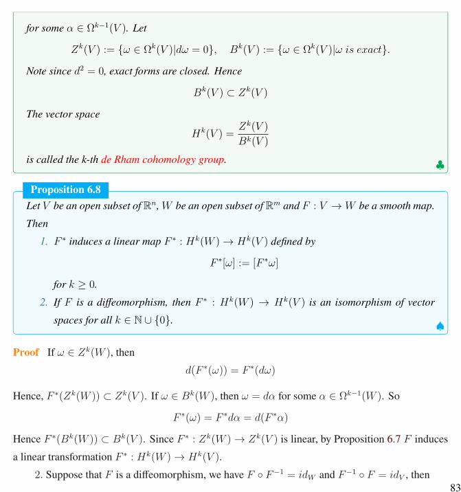
for some α ∈ Ωk−1(V ). Let
Zk(V ) := ω ∈ Ωk(V )|dω = 0, Bk(V ) := ω ∈ Ωk(V )|ω is exact.
Note since d2 = 0, exact forms are closed. Hence
Bk(V ) ⊂ Zk(V )
The vector space
Hk(V ) =Zk(V )
Bk(V )
is called the k-th de Rham cohomology group.
Proposition 6.8
♠
Let V be an open subset of Rn,W be an open subset of Rm and F : V → W be a smooth map.Then
1. F ∗ induces a linear map F ∗ : Hk(W )→ Hk(V ) defined by
F ∗[ω] := [F ∗ω]
for k ≥ 0.2. If F is a diffeomorphism, then F ∗ : Hk(W ) → Hk(V ) is an isomorphism of vector
spaces for all k ∈ N ∪ 0.
Proof If ω ∈ Zk(W ), thend(F ∗(ω)) = F ∗(dω)
Hence, F ∗(Zk(W )) ⊂ Zk(V ). If ω ∈ Bk(W ), then ω = dα for some α ∈ Ωk−1(W ). So
F ∗(ω) = F ∗dα = d(F ∗α)
Hence F ∗(Bk(W )) ⊂ Bk(V ). Since F ∗ : Zk(W )→ Zk(V ) is linear, by Proposition 6.7 F inducesa linear transformation F ∗ : Hk(W )→ Hk(V ).
2. Suppose that F is a diffeomorphism, we have F F−1 = idW and F−1 F = idV , then83

(F−1 F )∗ = F ∗ (F−1)∗ = (idV )∗ = idHk(V )
which implies that F ∗ is onto. From
(F F−1)∗ = (F−1)∗ F ∗ = (idW )∗ = idHk(W )
we see that F ∗ is one-to-one. Therefore, F ∗ is an isomorphism.
Proposition 6.9
♠If V ⊂ Rn is a nonempty connected open subset, then H0(V ) ∼= R.
Proof Note that B0(V ) = 0. For f ∈ Z0(V ),
df =n∑i=1
∂f
∂xidxi = 0
which means ∂f∂xi≡ 0 on V , for all i = 1, · · · , n. So grad(f) = 0 on V . By theorem, f is a constant
function on V . Hence Z0(V ) = R and
H0(V ) = R/0 ∼= R
Corollary 6.4
If V ⊂ Rn is an open subset which has k connected components, then
H0(V ) ∼= Rk
The following famous result says that all closed k−forms on Rn are exact.
Theorem 6.8. Poincaré lemma
For k ∈ N,Hk(Rn) = 0
84

Corollary 6.5
R2 − (0, 0) is not diffeomorphic to R2.
Proof Letω = − y
x2 + y2dx+
x
x2 + y2dy ∈ Ω1(R2 − (0, 0))
We have
dω = −(x2 + y2)− y(2y)(x2 + y2)2
dydx+(x2 + y2)− x(2x)
(x2 + y2)2dxdy
=(x2 − y2)(x2 + y2)2
dxdy − (x2 − y2)(x2 + y2)2
dxdy = 0
Let φ : [0, 1]→ R2 − (0, 0) be defined by
φ(θ) = (cos 2πθ, sin 2πθ)
Assume that w = dα for some α ∈ Ω0(R2 − (0, 0)). Then by Stokes’ theorem,∫ϕ
ω =
∫ϕ
dα =
∫∂ϕ
α = α(φ(1))− α(φ(0)) = 0
But ∫ϕ
ω =
∫ 1
0
− sin 2πθ
cos2 2πθ + sin2 2πθ(− sin 2πθ)(2π) +
cos 2πθ
cos2 2πθ + sin2 2πθ(cos 2πθ)(2π)dθ
=
∫ 1
0
2πdθ = 2π = 0
which is a contradiction. Therefore some closed 1-forms onR2−(0, 0) are not exact which impliesthat H1(R2 − (0, 0)) = 0. But by the Poincaré lemma, H1(R2) = 0, this proves the result.
85
Appendix 6.6
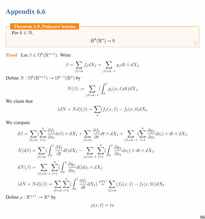
Theorem 6.9. Poincaré lemma
For k ∈ N,Hk(Rn) = 0
Proof Let β ∈ Ωk(Rn+1). Write
β =∑|I|=k
fIdXI +∑
|J |=k−1
gJdt ∧ dXJ
Define N : Ωk(Rn+1)→ Ωk−1(Rn) by
N(β) :=∑
|J |=k−1
(
∫ 1
0
gJ(x, t)dt)dXJ
We claim that(dN +Nd)(β) =
∑I
(fI(x, 1)− fI(x, 0)dXI
We compute
dβ =∑|I|=k
(n∑l=1
∂fI∂xl
dxl) ∧ dXI +∑|I|=k
∂fI∂t
dt ∧ dXI +∑
|J |=k−1
(n∑l=1
∂gJ∂xl
dxl) ∧ dt ∧ dXJ
N(dβ) =∑|I|=k
(
∫ 1
0
∂fI∂t
dt)dXI −∑
|J |=k−1
n∑l=1
(
∫ 1
0
∂gJ∂xl
dxl) ∧ dt ∧ dXJ
dN(β) =∑
|J |=k−1
n∑l=1
(
∫ 1
0
∂gJ∂xl
dt)dxl ∧ dXJ
(dN +Nd)(β) =∑|I|=k
n∑l=1
(
∫ 1
0
∂fI∂t
dXI)FTC=
∑|I|=k
(fI(x, 1)− fI(x, 0))dXI
Define ρ : Rn+1 → Rn byρ(x, t) = tx
86

where x = (x1, · · · , xn). Let L = N ρ∗. Then
Ld+ dL = Nρ∗d+ dNρ∗ = Ndρ∗ + dNρ∗ = (Nd+ dN)ρ∗
Let ω = hdXI ∈ Ωk(Rn), I = (i1, · · · , ik)
ρ∗(hdXI) = (ρ∗h)(ρ∗dXI) = h(tx)dρI
Note that
dρI = dρi1 ∧ · · · ∧ dρik = d(txi1) ∧ · · · ∧ d(txik) = (tdxi1 + xi1dt) ∧ · · · ∧ (tdxik + xikdt)
= tkdXI + terms that include dt
Henceρ∗(hdXI) = h(tx)(tkdXI + terms that include dt)
Then
(Nd+ dN)ρ∗ω = (Nd+ dN)ρ∗(hdXI) = (h(1x)1k − h(0x)0k)dXI = h(x)dXI = ω
By linearity, for all ω ∈ Ω(Rn),(Nd+ dN)ρ∗ω = ω
If dω = 0, thenω = (Nd+ dN)ρ∗ω = Nρ∗dω + d(Nρ∗ω) = d(Nρ∗ω)
Hence ω is exact and therefore Hk(Rn) = 0, for all k > 0
87

88

Bibliography
[1] Marsden J. and Hoffman M.J., Elementary classical analysis, 2nd ed., Freeman, New York, 1993.[2] Pugh, C.C., Real mathematical analysis, Springer-Verlag, New York, 2002.[3] Rudin, W., Principles of mathematical analysis, 3rd edition, McGraw-Hill, New York, 1985.
Index
Absorbing barrier, 4Adjoint partial differential operator, 20A-harmonic function, 16, 182A∗-harmonic function, 182
Boundary condition, 20, 22Dirichlet, 15Neumann, 16
Boundary value problemthe first, 16the second, 16the third, 16
Bounded set, 19
Diffusioncoefficient, 1equation, 3, 23
Dirichletboundary condition, 15boundary value problem, 16
Ellipticboundary value problem, 14, 158partial differential equation, 14
partial differential operator, 19
Fick’s law, 1Flux, 1Formally adjoint partial differential operator,
20Fundamental solution
conceptional explanation, 12general definition, 23temporally homogeneous case, 64, 112
Genuine solution, 196Green function, 156Green’s formula, 21
Harnack theoremsfirst theorem, 185inequality, 186lemma, 186second theorem, 187third theorem, 187
Helmhotz decomposition, 214Hilbert-Schmidt expansion theorem, 120
Initial-boundary value problem, 22

Initial condition, 22Invariant measure (for the fundamental
solution), 167
Maximum principlefor A-harmonic functions, 183for parabolic differential equations, 65strong, 83
Neumannboundary condition, 16boundary value problem, 16function, 179
One-parameter semigroup, 113
Parabolic initial-boundary value problem, 22Partial differential equation
of elliptic type, 14of parabolic type, 22
Positive definite kernel, 121
Reflecting barrier, 4Regular (set), 19Removable isolated singularity, 191Robin problem, 16
Semigroup property (of fundamentalsolution), 64, 113
Separation of variables, 131Solenoidal (vector field), 209Strong maximum principle, 83Symmetry (of fundamental solution), 64, 112
Temporally homogeneous, 111
Vector field with potential, 209
Weak solutionof elliptic equations, 195of parabolic equation, 196associated with a boundary condition, 204
91