Advanced Auction Theory

IEOR 298 Supply Chain ManagementApril 22, 2005

Nick RosicShehzad Wadalawala

Juan Wang

Presentation Outline

Introduction to Auctions

Reverse AuctionsRules and ProceduresCase: Smart Markets

BREAK

Advanced Forward AuctionsVickrey Clarke Grove MechanismSimultaneous Ascending AuctionCase: FCC Spectrum

Double Auction

Introduction to Auctions• An auction is a method of allocating scarce

goods,– A seller wishes to obtain as much surplus as possible, – A buyer wants to pay as little as necessary.

• An auction is a simple way of determining allocations and prices.

• Auctions have the quality of being “fair”– Any bidder has a chance to win if his bid is sufficient

• An auction is “efficient” when objects are: – Allocated to those bidders who value them most;

• The price is determined by the bids.

Application of Auctions

• Auctions are useful when – the goods do not have a fixed or determined market

value, in other words, when a seller is unsure of the price he can get.

• Choosing to sell an item via auction is – more flexible than fixing the price;– less time-consuming and expensive than negotiating

a price.– Usually earns greater revenue

• Auctions can be used – for single items such as real estate or works of art;– and for multiple units of a homogeneous item such as

gold or Treasury securities.

Information Extraction• The price is determined by the bidders. • The seller controls the auction type. • The auctioneer is usually a third party

that acts as an agent for an object owner. • The buyers frequently know more than

the seller about the value of the item. • A seller, not knowing the true value of an

object would rather let the informed bidders determine price than suggest a price out of fear that his ignorance will prove costly.

Bidder Valuations• Private valuation

– Bidders valuations do not depend on others, in literature often the bids are assumed as iid (independent and identically distributed), when is this a reasonable assumption?

– All bidders have private valuations and tend to keep that information private.• The surplus that a bidder obtains through an

auction is sometimes referred to as his information rent.

*Most models assume IPV (Independent Private Valuation)

Bidder Valuation (cont)• Common valuation

– Goods are acquired goods for resale or commercial use;

– An individual bid is based not only upon a private valuation but also upon an estimate of market value of the object after the auction. Each bidder tries to guess the ultimate price of the item.

– The item is really worth the same to all, but the exact amount is unknown

• Example– Purchasing land for oil drilling

• Each bidder has different information and a different valuation, but the value of the oil is common.

Winner’s Curse• In common value auctions, bidders must be

concerned about the "Winners curse." • Bidders go to auctions to win, but in common

value auctions, the "lucky" winner pays more for an item than it is worth. Auction winners are faced with the sudden realization that their valuation of an object is higher than that of anyone else.

• How can bidders adjust for the winner’s curse?

• Bidders who estimate value correctly do not win in common value auctions

Auction Formats

• Traditional Auction Formats– English– Dutch– First Price Sealed Bid– Vickrey Second Price Sealed Bid

Auction Formats (cont)

• Alternative Auction formats– Reverse Auction– Simultaneous Ascending Auction – Double Auction– Anglo-Dutch– Clock Auction

Introduction to Reverse Auctions

• In contrast to many consumer auctions, a reverse auction involves one buyer and many sellers.

• A reverse auction is descending in price. Sellers place bids on the desired item, and the lowest bid wins. In order to achieve a positive payoff, each seller cannot bid below its valuation of the item.

Reverse Multi-item Auctions for Industrial Procurement

• In this type of auction, an industrial organization seeks to buy a bundle of goods from many different suppliers.

• As a reverse auction, the auction is descending in price. Suppliers place bids on the desired bundle of goods, and the lowest bid for each item wins.

• The buyer can purchase different goods from different suppliers. Because of capacity constraints, the buyer may also need multiple suppliers to provide a single good.

• In order to receive a positive profit, suppliers cannot bid below their production cost for a particular good. Therefore, the supplier with the lowest production cost can outbid its competitors.

Smart Markets for Auctions• Definition: A smart market is an exchange institution in

which a computer uses an optimization algorithm to solve the allocation problem associated with each set of bids.

• Bidding Process:– Before making any bids, suppliers submit their production costs

to the computer program.– Suppliers place initial bids on the given bundle of goods.– The computer program inputs these bids, then computes the

allocation which minimizes the buyer’s total cost.– Each supplier is informed of what its allocation would be given

the current bids.– The program also outputs to each supplier a best response bid

for the next round.– The next round of bidding begins, and suppliers are free to

change their bids.– The auction continues until all suppliers’ bids are unchanged in

consecutive rounds.

Quantitative Auction Model

• Basic problem: A large manufacturing company would like to buy a certain quantity of m different components, and n suppliers compete to offer the lowest selling prices for these components.

• Each supplier has a unique set of production constraints; a given supplier may not be able to offer the entire desired quantity of a good.

• Variables– qj = buyer’s requested quantity of component j– ci = total amount of production resource available to supplier i– aij = amount of resource needed for supplier i to produce one unit of

component j – bij (t) = unit price bid by supplier i for component j in round t (this bid can be for any quantity between 0 and qj) – xij (t) = supplier i’s potential allocation of component j in round t – vij = supplier i’s unit production cost for component j

Bidding Rules

• 1. Non-reneging rule: The supplier may not increase a previous bid for any component. – Mathematically, this means that bij (t) < bij (t’)

for any t’ < t.

• 2. Common multiple rule: All bids must be integer multiples of ε for some ε > 0. – Therefore, there is a minimum bid decrease

of ε.

The Buyer’s Minimization Problem

• Given a particular set of bids b(t) and desired set of quantities q, the buyer seeks to minimize the total cost of purchasing the bundle q.

• Mathematically, we have: min Σi Σj bij(t)*xij

s.t. Σj aij*xij < ci for all i

Σi xij = qj for all j

xij > 0 for all (i,j)

Supplier’s Payoff Problem• Each supplier seeks to maximize its profits given its own

capacity and production costs and the bids of its competitors.

• Supplier i’s potential payoff in a given round of bidding is:

πi (b(t)) = Σj (bij(t) – vij)*xij(t)

• Unfortunately for suppliers, the quantities xij(t) are unknown when bids are submitted for round t. Under the MBR assumption, however, the supplier can calculate estimates of these quantities based on the current bids of competitors.

Myopic Best Response Model

• The best response bids calculated in the smart market are called myopic best response (MBR).

• Under MBR, a supplier’s potential profit in the next round of bidding is maximized, given that all bids of competitors are unchanged.

• This assumption is extremely unrealistic, given that many suppliers will probably change their bids in order to improve their payoffs. So, an MBR bid can often produce a suboptimal result for a given supplier.

Smart Market Information Structure

• The buyer knows:– Supplier identities– Capacity constraints of all suppliers– All bids– Potential allocation at the end of each round

• The buyer does not know:– Suppliers’ production costs– MBR suggested bids

• Each supplier knows:– Desired quantities of the buyer– Its own potential allocation– Its own MBR suggested bid

• Each supplier does not know:– Identities of other suppliers– Capacity constraints and production costs of competitors– Competitors’ bids– Competitors’ potential allocations and MBR suggested bids

Deficiencies of the Model

• As explained previously, the MBR assumption will most likely not provide the optimal bids for a given supplier.

• The model assumes that production costs are linear. This is quite inaccurate, since suppliers can often use economies of scale to lower their average production costs.

• In addition, the costs of producing one component may be affected by whether company produces other components. The model does not consider interactions between goods.

Basic Results• At first, we make only a weak behavioral assumption: if a supplier

receives a potential allocation of zero for all components, it will lower its bid, unless a decreased bid would produce a negative profit.

• With this simple assumption, the following result holds:

Proposition: Let T be the final round of the auction, let v1:nj, …,

vn:nj be the order statistics of (v1j, …, vnj), and define PC = {i Є {1,

…, n}, xi(T) = 0}. Provided that |PC| > 1 and under the weak behavioral assumption, we have

xij(T) > 0 → bij(T) < vn-|Pc|+1:n + ε for all j Є {1, …, m}.

• So, the buyer is guaranteed a maximum level of bids given the production costs of the suppliers. This upper bound depends heavily on how many suppliers are shut out of the final allocation.

MBR Behavioral Model

• Suppose that each bidder follows its MBR suggestion in every round of bidding.

• This means that bids in every round are completely determined by the initial set of bids and the suppliers’ production costs, since the suppliers do not actually make any decisions once they have submitted their first round bids.

• Proposition: Let (b(t))tЄN be a myopic best response bidding sequence defined by a set of initial bids b(0) and the recursive relation b(t+1) = F[b(t)]. Then, there exists an integer T > 0 such that b(t) = b(T) for all t > T.

• Proof: All bids are non-decreasing and have a lower bound of zero. The common multiple rule implies that bids can only take on a finite set of values. So, the bidding sequence must converge in a finite number of steps.

A Sample Auction

• Consider the case where n=2, m=1. That is, there are two suppliers competing for one component.

• If the suppliers’ constraints are low enough, the buyer will need to purchase some amount from both suppliers.

• In this case, if the initial bids are very far apart, there may be a premature equilibrium. If the higher bidder outbids the lower one, the increase in volume might not make up for the loss in price.

• The buyer may be able to prevent premature equilibria by requiring a maximum initial bid, since this requirement will encourage suppliers to bring their bids closer together.

Dynamic 2x2 Auction

Summary

• 1. For industrial procurement auctions in which the capacity constraints of suppliers are known, a “smart market” computer program can find the optimal allocation of components to minimize the buyer’s total cost. – With an effective information structure in place, the smart market

is able to limit collusion.

• 2. Even when we make a very simple behavioral assumption, we can derive upper bounds for the suppliers’ bids, so the buyer’s total cost is also bounded.

• 3. If all suppliers follow the myopic best response suggestions, the outcome of the procurement auction is fully determined by the opening bids.– When opening bids are very far apart, the auction may converge

quickly to a premature equilibrium.– The buyer can impose a maximum initial bid to prevent this

occurrence.

Possible Improvements

• Nonlinear production costs• More complicated capacity constraints• Alternative behavioral models• Inclusion of decision-making factors

other than price– Switching costs between suppliers– Historical preferences and supplier

reputations– Quality measure for components

Other Examples of Reverse Auctions

• Sears Logistic Services (SLS) writes contracts with trucking companies to provide shipping services for Sears department stores.

• In 1992, SLS worked with the consulting firm JSCO in attempts to lower the costs of its trucking contracts. – JSCO designed a reverse auction in which suppliers

could place all-or-nothing bids on bundles of lanes.– SLS’ shipping costs dropped from $190 million per

year to $165 million per year, a savings of $25 million, or 13%.

Other Examples

• The U.S. Navy hired Freemarkets in 2000 to hold a procurement auction for the parts of airplane ejection seats. The Navy was able to save 29% from its traditional costs.

• PriceLine.com uses reverse auctions to find inexpensive hotels and flights for travelers.

Vickrey-Clarke-Groves (VCG) Auction

A Lovely in Theory but lonely in Practice Mechanism

Background

• Generalization of the second price sealed bid auction of Vickrey Auction (1961) by Clarke (1971)and Groves (1973)

• Vickrey Auction:– a single type of goods, bidders report demand schedule for

“all possible quantities”– Auctioneers then select the allocation to maximize the total

value– Each bidder pays the lowest total bid that buyer could have

made to win its part of the final allocation, given the other bids

– Vickrey proved Dominant strategy property, efficient allocation

• VCG:– Dominant strategy property still holds when extending to

many types of goods– bidders make bids on “all possible packages”– The allocation still assigns goods efficiently– charges bidder opportunity costs of the item they win

Uniqueness and Equivalence Results

• Uniqueness: Green and Laffont (1979) and Holmstrom (1979)– Any efficient mechanism with the dominant

strategy property, and in which losers have zero payoffs is equivalent to the VCG mechanism, in the sense of leading to identical equilibrium outcomes.

• Revenue Equivalence: Williams (1999)– All Bayesian mechanisms that yield efficient

equilibrium outcomes and in which losers have zero payoffs lead to same expected equilibrium payments as the VCG mechanism.

• Important theoretical foundation of auction design

VCG Mechanism in Formal Language

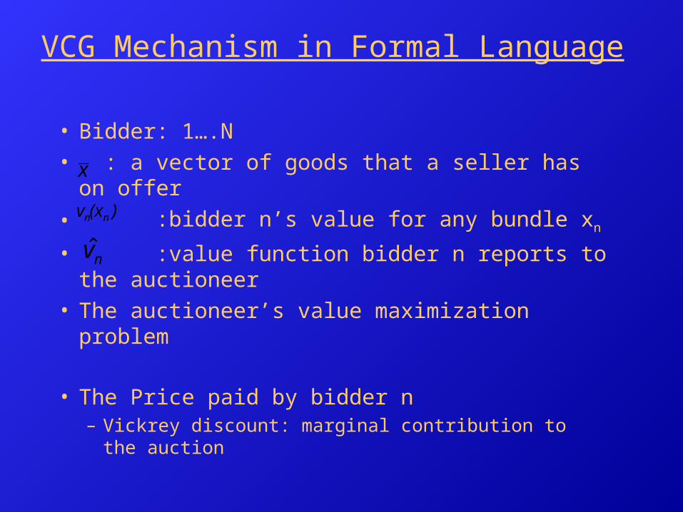
• Bidder: 1….N• : a vector of goods that a seller has on

offer

• :bidder n’s value for any bundle xn

• :value function bidder n reports to the auctioneer

• The auctioneer’s value maximization problem

• The Price paid by bidder n– Vickrey discount: marginal contribution to the

auction

x

)(xv nn

nv̂

An Example of VCG Auction• Real valuations for

different bundlesA B AB

Agent 1

3 4 12

Agent 2

5 5 5

Agent 3

6 2 10

• Bids for different bundles

A B AB

Agent 1 2 3 7

Agent 2 5 4 *

Agent 3 5 1 6

• Winning allocation: – A->3; B->2 (XOR bids)

• Payments of Agent 2 and agent 3?• What if bidding true value?

Dominant Strategy in VCG Mechanism

• Theorem: Truthful reporting is a dominant strategy for each bidder in the VCG mechanism. Moreover, the outcome of the mechanism is one that maximizes total value.

• Proof:

Virtues of the VCG Mechanism

• Dominant-strategy Property– Reduce the cost of auction

• Easy for the bidders to determine their optimal bidding strategy

• Eliminate bidder’s incentive to spend resources learn other bidders value

– Efficient prediction is reliable

• Scope of application– No restrictions on the possible ranking of different

outcomes– Allow auctioneer to impose some extra constraints– Replaces by other constraints of the

form x Є X without changing Theorem 1&2 in any essential way

xxm m

Why Practical Application of VCG are rare?

• Revenues can be very low or zero– Example

– What is the revenue?– 0!!!– The revenue deficiency of VSG mechanism

is decisive to reject it for most practical applications

A B AB

Agent 1

* * 2

Agent 2

2 * *

Agent 3

* 2 *

Shill bidding and Collusion• Shill bidding: submit additional bids under false

identities

– Winning bid? Payment?– Bidder 1 wins, pays 1 – Bidder 2 bids as bidders 2 and 3, submits 2 for one item

• Dominant strategy property depends on unlimited budget– Example? Homework!!

• Privacy preservation problem

A B AB

Agent 1

* * 2

Agent 2

0.5

0.5

1

Simultaneous Ascending Auctions

A Successful Practical Mechanism

Brief History• First use: sell licenses to use bands of radio

spectrum in 1994 by FCC in US• Motivation:

– Reduce Federal regulation of radio spectrum• Main rules from two detailed proposals:

– Preston McAfee– Robert Wilson and Paul Milgrom

• Success– Employed by the FCC in almost all US radio spectrum

auctions• US $617 million sale of ten paging licenses in July 1994

– Adopted with slight variations for dozens of spectrum auctions worldwide, >$200 billion

• Early auctions in Europe for 3G mobile wireless licenses ~$100 billion

– Extended to the sale of divisible goods in electricity, gas and environmental markets

Introduction

• Usually for a group of items with strong value interdependency– Aggregation of licenses is important to achieve

efficiency

• Natural generalization of English Auction– Multi-round, simultaneous

• Not combinatorial auctions– Bidders are not allowed to bid on packages

• A useful benchmark for comparison of Combinatorial Auctions

SAA Rules

• Each round, bidders simultaneously make sealed bids for any item

• Round results are posted after each bidding.– identities of new bids and bidders for each item– “standing high bid” and the corresponding bidder

• Minimum bids for the next round– “standing high bid”+ predetermined bid increment

• Activity rule– Requires bidder maintain a minimum level of activity to

preserve its current eligibility– Considered as active if it makes an eligible new bid or

owns the standing high bid– Create pressure on bidders to bid actively, increase

pace of auction– Increase the information available to bidders, improve

price discovery

SAA Rules Continued

• Stopping rule– Bidding on all licenses closes simultaneously

where there is no new bidding on any license

• Payment/Allocation rule– Allocate the standing high bids to the

corresponding bidders at the price equal to the bids

• Bid withdrawal– Withdraw penalty: max{0, withdrawn bid-

final sale price }

Performance of SAA

• Example :Three US PCS broadband auction– Revenue– Generate market price?

• Results:– Narrowband auctions: a few percent and often zero– First broadband auction: price difference <1 minimum

bid increment in 42 out of 48 markets• Compared with Sequential Auction

– Swiss wireless-local-loop auction in March 2000: 3 nationwide licenses, first two 28 MHz blocks for 121 and 134 million francs, third one 56 MHz for 55 million francs

– Efficient license aggregation?• bidders appear to piece together sensible license

aggregation– Efficient?

• Absence of resale

Why Success?

• Excellent Price discovery– simultaneous rather than sequential

• In sequential auctions, bidder must guess what prices will be in future auctions when determining bids in the current auction

– Multi-round:• Bidders see tentative price info. at each round, winner’s

curse reduced

– Price info. helps bidders focus valuation efforts in the relevant range of price space----discovering values is costly

– Bidders retain sufficient flexibility to shift towards their best package

• Problems?

Demand Reduction

• Definition:– When multiple items are sold through the use of a SAA,

bidders can find it in their mutual interests to reduce their aggregate demand for the items while prices are still below the bidders' valuations

• Example:

• The bidder prefers winning one unit at low prices than winning two items at a price high enough to outbid the other bidder, not efficient equilibrium

• 1999 German GSM spectrum auction, lasted just two rounds

• Nationwide broadband auction, the largest bidder, PageNet, reduced its demand from 3 to 2, when prices < its marginal value

A B AB

Agent 1 3 3 6

Agent 2 2 2 2

No Competitive Equilibrium Exists

• Theorem: suppose that the set of possible individual valuation functions includes both mutual substitutes in individual demand, and at least one other valuation function, then if there are at least two bidders, there is a profile of possible individual valuation functions such that no competitive equilibrium exists.

• Parking Spots Auction:

– Unique value maximizing license allocation?– Why no equilibrium?

• For it to happen, PA>=75 and Pb>=75

A B AB

Agent 1

0 0 100

Agent 2

75 75 75

Exposure Problem• With individual bidding, a bidder may fail to acquire

key pieces of the desired combination, but pay prices based on the complementary gain.

• Exposure problem results in inefficiency– Netherlands DCS-1800 auction in February 1998– 18 licenses for sale, A and B efficiently scaled, 16 too small

to be useful for a mobile phone business alone, need to be combined

– final price per unit in A and B >2 times those for any of the small lots

• Parking Spots Example– if the first bidder drops out early, result?

• Allowing package bidding partially solves the problem– Result?

• Withdrawal of bids mitigates the exposure problem• Usually complementarities are not extreme and

competition is greater

Ascending Auctions with Package Bidding

L.M. Ausubel and P.R MilgromFrontiers of Theoretical Economics,

1(1): 1-50, 2002

Double Auctions

• Double auctions are closest to reflecting natural marketplaces

• Many buyers and many sellers• Examples

– Covisint• http://www.isa.org/InTechTemplate.cfm?Section=Article_Ind

ex&template=/ContentManagement/ContentDisplay.cfm&ContentID=8342

• 2001 Daimler Chrysler held a reverse auction with spending of $2.5 billion

• What is the effect on buyer supplier relationships?

Emission Permits

“The vast majority of the world’s climate scientists have concluded that if the countries of the world do not work together to cut the emission of greenhouse gases, then temperatures will rise and will disrupt the climate. In fact, most scientists say the process has already begun.”

– President Clinton, October 22, 1997– 1246 million metric tons of permits each year– Typically marginal price is $100, equivalent to $125 billion

if auctioned efficiently•Kyoto Protocol•US uses “grandfathering” instead of auctions for allocation of

permits

Types of Double Auctions

• Call Auction– All bids are submitted to a third party

that matches supply and demand and clears the market

• Continuous Auction– At any time a bidder and supplier can

agree to a price and quantity and transact

• Why one over the other?

Objectives of Double Auction Design

• Truthful Revelation (Strategy proofness)

• Efficiency• Budget Balance• Individual Rationality (Participation

Constraint)• Myerson and Sattherthwaite (1983)

prove that it is impossible to have all four for the double auction

The allocation problem

),(}1,0{

}1,0{

}1,0{

max

JjIiz

Jjy

Iix

Jjyz

Iixz

st

ygxf

ij

j

i

ijij

ij

ij

jjj

iii

Vickrey Model for the Double Auction

•Efficient Outcome

•Truthful Revelation

•Individually Rational

•NO BUDGET BALANCE

Example

I = 3, N = 3

f = (300, 250, 200), g = (175, 225, 275)

Tug of WAR!

Keeping the peace

• If we relax the need to maximize efficiency, we can obtain truthful revelation

• Eliminate the least profitable trade from the allocation

• Bidders pay price equal to newly rejected bidder’s price and suppliers are paid newly rejected bidder’s ask price.

Multi-unit demand/Multi-unit supply• In multi-unit demand and multi-unit

supply case, prices are discriminatory.• Demand Reduction

– Bidder 1 f = (10, 3)– Bidder 2 f = (7)– Supplier 1, g = (2)– Supplier 2, g = (2)

• Concerns about fairness• Supply Reduction is similar

Future Directions

• Combinatorial Auctions• Multi-attribute Auctions

• Questions?

Sources

• An, N., Elmaghraby, W., and Keskinocak, P., 2004, “Bidding Strategies and their Impact on Revenues in Combinatorial Auctions,” Georgia Institute of Technology.

• Ausubel, L, Cramton, P., 2002, “Demand Reduction and Inefficiency in Multi-Unit

Auctions,” University of Maryland, Working Paper 9607, revised July 2002.

• Chu, L, Shen, Z., 2003, “Agent Competition Double Auction Mechanism”

• Cramton, P., Shoham, Y., and Steinberg, R. (editors), 2006, Combinatorial Auctions, forthcoming, MIT Press.

• Dayama, P. and Narahari, Y., “Combinatorial Auctions for Electronic Business.”

More Sources• Gallien. J., and Wein, L., 2000, “Design and Analysis of a

Smart Market for Industrial Procurement,” Massachusetts Institute of Technology.

• Hardy, Michael, 2003, “Reverse auctions save Navy millions,” fcw.com.

• Milgrom, P., “Putting Auction Theory to Work: The Simultaneous Ascending Auction.”

• Sunnevag, K., 2001, “Auction design for the allocation of emission permits”

• Vries, S, Vohra, R., 2001, “Combinatorial Auctions: A Survey”