addendum to the pest manual - aquaveogmsdocs.aquaveo.com/pest addendum.pdfaddendum to the pest...

Addendum to the

PEST Manual

John Doherty

Watermark Numerical Computing

April 2005

Table of Contents

Table of Contents 1. Introduction............................................................................................................................1 2. Alterations and Upgrades to PEST ........................................................................................2

2.1 New Restart Option.........................................................................................................2 2.2 Template and Instruction File Headers ...........................................................................3 2.3 User Intervention.............................................................................................................3 2.4 Improvements to the Predictive Analyser .......................................................................4 2.5 Switch to Three-Point Derivatives Calculation ..............................................................5 2.6 Alterations to SVD-Assist Functionality ........................................................................6 2.7 A New IREGADJ Option................................................................................................8

3. Alterations and Upgrades to PEST Utilities ........................................................................11 3.1 JCO2JCO.......................................................................................................................11 3.2 PCLC2MAT..................................................................................................................11

4. Model Predictive Error Analysis .........................................................................................16 4.1 Concepts........................................................................................................................16

4.1.1 General ..................................................................................................................16 4.1.2 Calculation of the R and G Matrices.....................................................................17 4.1.3 Some Special Considerations ................................................................................19

4.2 Alterations to PEST ......................................................................................................20 4.2.1 The IRES Variable ................................................................................................20 4.2.2 The “Resolution Data File” ...................................................................................20

4.3 RESPROC.....................................................................................................................21 4.3.1 General ..................................................................................................................21 4.3.2 What RESPROC Does ..........................................................................................21 4.3.3 Running RESPROC ..............................................................................................22 4.3.4 SVD-Assisted Parameter Estimation ....................................................................22

4.4 RESWRIT .....................................................................................................................23 4.4.1 General ..................................................................................................................23 4.4.2 Running RESWRIT...............................................................................................23 4.4.3 Format of Matrix Files ..........................................................................................24

4.5 PARAMERR.................................................................................................................25 4.5.1 General ..................................................................................................................25 4.5.2 Uncertainty Files ...................................................................................................25 4.5.3 Using PARAMERR ..............................................................................................28

4.6 PREDERR.....................................................................................................................29 4.6.1 General ..................................................................................................................29 4.6.2 Using PREDERR ..................................................................................................29

4.7 OBSREP........................................................................................................................30 4.7.1 General ..................................................................................................................34 4.7.2 Running OBSREP .................................................................................................34

Table of Contents

4.8 PCOV2MAT .................................................................................................................35 4.8.1 General ..................................................................................................................35 4.8.2 Using PCOV2MAT...............................................................................................36

4.9 MATRIX MANIPULATION PROGRAMS ................................................................36 4.9.1 General ..................................................................................................................36 4.9.2 JROW2MAT .........................................................................................................37 4.9.3 JROW2VEC ..........................................................................................................37 4.9.4 MAT2SRF.............................................................................................................38 4.9.5 MATADD .............................................................................................................39 4.9.6 MATCOLEX.........................................................................................................39 4.9.7 MATDIFF .............................................................................................................39 4.9.8 MATPROD ...........................................................................................................39 4.9.9 MATQUAD...........................................................................................................40 4.9.10 MATROW...........................................................................................................40 4.9.11 MATSMUL.........................................................................................................41 4.9.12 MATSVD ............................................................................................................41 4.9.13 MATSYM ...........................................................................................................42 4.9.14 MATTRANS.......................................................................................................42 4.9.15 PEST2VEC..........................................................................................................42 4.9.16 VEC2PEST..........................................................................................................43 4.9.17 VECLOG.............................................................................................................44

Introduction 1

1. Introduction This document describes alterations to PEST that have been make since publication of the latest edition of the PEST manual (i.e. the fifth edition of the manual). Publication of the fifth edition of the manual coincided with the release of version 9.0 of PEST. Hence all alterations documented herein pertain to versions later than that.

Alterations and Upgrades to PEST 2

2. Alterations and Upgrades to PEST 2.1 New Restart Option Execution of PEST can now be recommenced with four different switches. Use of the “/r”, “/j” and “/s” switches is documented in the PEST manual. The new restart switch is the “/d” switch.

The “/d” switch has a similar role to the existing “/s” switch. Recall that the “/s” switch can be used to recommence Parallel PEST execution at the same model run in which it was previously interrupted, if interruption took place during calculation of the Jacobian matrix. If Parallel PEST execution was interrupted during the Marquardt Lambda testing procedure however, restarting PEST with the “/s” switch has the same effect as restarting it with the “/j” switch; that is, PEST is restarted at that point in its previous run at which calculation of the Jacobian matrix was just completed.

If PEST is run in non-parallel mode, then it cannot be restarted with the “/s” switch. However it can be re-started with the “/d” switch. The effect is exactly the same as re-starting a Parallel PEST run with the “/s” switch.

Note the following important points pertaining to PEST’s restart switches:-

1. Parallel PEST cannot be restarted with the “/d” switch.

2. Non-Parallel PEST cannot be restarted with the “/s” switch.

3. A previously stopped Parallel PEST run can be restarted as non-Parallel PEST or Parallel PEST using either the “/r” or “/j” switches.

4. A previously stopped non-Parallel PEST run can be restarted as Parallel PEST using either the “/r” or “/j” switches.

5. A previously stopped Parallel PEST run cannot be restarted as non-Parallel PEST with the “/s” switch.

6. A previously stopped non-Parallel PEST run cannot be restarted as Parallel PEST with the “/d” switch.

The reader is probably wondering at this stage why, if the “/s” and “/d” switches have the same effect, they cannot be used interchangeably between Parallel and non-Parallel PEST. The reason is that run management is very different between these two versions of PEST. For Parallel PEST, runs are not necessarily undertaken in sequence. Run results in the restart file are also not stored in sequence. For non-Parallel PEST, the restart file does not hold run results; rather it holds fragments of the Jacobian matrix; this can save considerably on file storage when central differences are used for derivatives calculation. Also, this restart methodology is more easily combined with external derivatives calculation – this being available only in the non-Parallel version of PEST at present.


It is freely admitted however, that an all-purpose run manager is needed. This, hopefully, will be one an outcome of future PEST development. At that stage the “/s” and “/d” switches will be combined.

2.2 Template and Instruction File Headers The first line of a template file must be:- ptf #

where “#” can be replaced by any other character that is suitable for definition of a parameter delimiter. “ptf” stands for “PEST template file”.

The first line of an instruction file must be:- pif #

where “#” can be replaced by any other character that is suitable for use as a marker delimiter. “pif” stands for “PEST instruction file”.

PEST and its checking utilities now allow alternative headers for these two files. “jtf” (for “JUPITER template file”) can be used in place of “ptf” and “jif” (for “JUPITER instruction file”) can be used in place of “pif”.

2.3 User Intervention The “parameter hold file” can be used to hold the values of certain parameters fixed. By stopping and restarting PEST using the “/j” switch, an attempt can then be made to re-calculate the parameter upgrade vector with troublesome parameters temporarily deactivated.

As is explained in the PEST manual, the parameter hold file can be used not just for holding parameters fixed, but also for altering the values of certain control variables. At the time of writing, control variables for which in-flight alterations are thus allowed are LAMBDA, RELPARMAX, FACPARMAX and UPVECBEND.

Five new control variables can now be altered through the parameter hold file. These all pertain to the predictive analysis process. They are INITSCHFAC, MULSCHFAC, NSEARCH, RELPREDSTP and ABSPREDSTP.

The first three of these variables govern the operation of the line search procedure used in prediction maximisation/minimisation. On many occasions, use of this procedure is critical to the success of the maximisation/minimisation process. Contrary to advice initially supplied with PEST documentation, it is often best to start this procedure with a low INITSCHFAC value (for example 0.2). However if it is set too low, this can result in wasted model runs. Similarly, MULSCHFAC may need to be set lower than 2.0 for highly nonlinear cases (even as low as 1.3). As this may require increased runs per line search, NSEARCH may need to be set higher than normal.

It is not explained in the PEST manual that termination criteria for the line search are the same as those for termination of the predictive analysis process as defined by the RELPREDSTP and ABSPREDSTP variables. (Actually, the line search procedure follows a


complex algorithm in which both the objective function and prediction value are monitored, with the former often expected to fall and then rise along the path of the search; hence there are, in fact, a number of other termination criteria required for implementation of this algorithm). It has been found from experience that in difficult problems, RELPREDSTP and ABSPREDSTP may need to be set quite low. This will be particularly important where small predictive uncertainty exists in a large predictive number (in which case the absolute, rather than the relative, termination criterion should be used), especially where line search increments are chosen to be small for better accommodation of nonlinear models.

New values for the above predictive analysis control variables can be supplied through the parameter hold file in the same way as for other variables. Figure 1 shows a file in which new values are provided for all of them.

As discussed in the PEST manual, the parameter hold file must be named case.hld where case is the filename base of the pertinent PEST control file. The hold file is read just after calculation of the Jacobian matrix and just before calculation of parameter upgrades. It is very important that a parameter hold file be deleted after use; this will prevent its contents being inadvertently used on a subsequent PEST run.

2.4 Improvements to the Predictive Analyser Considerable improvements have been made to the line search implemented by PEST’s predictive analyser. Recall from the PEST manual that implementation of a line search to find the highest/lowest prediction for which the objective function is at or lower than the user-supplied limit is optional; it is implemented only if NSEARCH is set to a number greater than 1. It has been found, however, that use of this option can greatly increase PEST’s ability to find the maximum constrained predictive value, especially in difficult numerical circumstances such as those that prevail where parameters are large in number and are highly correlated. The line search algorithm implemented by PEST is actually quite complicated, for not only does PEST need to monitor the value of the prediction as it travels along a certain parameter trajectory; it must also monitor the value of the objective function as well; on many occasions the objective function may actually fall before it rises to PD0 (the user-defined objective function limit) when travelling along the parameter upgrade line from the current set of parameter values to a potential new set of values.

It has been found that in those situations where numerical complexity dictates that a line search is warranted, it is worth doing this line search thoroughly. To optimise the efficacy of this search, the following settings are suggested.

• Set INITSCHFAC (initial line search factor) to 0.2 or 0.3; thus the line search begins at a point on the potential parameter upgrade line which is not too far from current parameter values.

initschfac 0.2 mulschfac 1.5 relpredstp 1.0e-4 abspredstp 0.00

Figure 1. Example of a parameter hold file.


• Set MULSCHFAC (line search factor multiplier) between 1.3 and 1.7.

• Set NSEARCH (maximum number of model runs devoted to the line search) to 15.

• Set PD1 quite close to PD0, maybe only 0.2% or less higher.

• Set ABSPREDSTP and RELPREDSTP reasonably tight. (These are actually the termination criteria for the predictive analysis process; one tenth of these values is also used for termination of the line search.)

• Start the predictive analysis process from optimised parameter values (for which the objective function is less than PD0).

Because the line search is repeated for every different value of the Marquardt lambda tested, it can consume an inordinate number of model runs if significant Marquardt lambda adjustment is warranted. Code has been inserted within PEST that aims to reduce the number of line search runs required when testing Marquardt lambdas after the first on any one optimisation iteration. Nevertheless, any savings that can be made in reducing trial Marquardt lambdas will result in increased efficiency. Thus after you have had experience with using the predictive analyser on your particular task, you may wish to consider setting the initial Marquardt lambda (RLAMBDA1) lower or higher than you normally would, if this is where PEST seems to prefer its value to be. Alternatively, set NUMLAM to 1, so that only 1 Marquardt lambda is employed per optimisation iteration; if this strategy is adopted it is probably good practice to try a very low value for RLAMBDA1, maybe in the vicinity of 0.01 to 0.001 (or even zero), and to start the predictive analysis process from previously-optimised parameter values.

While conducting a line search is a very time-consuming activity, experience has shown that it can be worth the effort in many circumstances; it is sometimes quite surprising how high or low calibration-constrained predictions can be. The cost of finding these extreme predictions, however, can be particularly high when using Parallel PEST to undertake the predictive analysis process, because while Jacobian runs are parallelised, line search runs are not. It is planned, however to partially parallelise this process in the future.

2.5 Switch to Three-Point Derivatives Calculation A new variable has been introduced to the “control data” section of the PEST control file in order to provide more flexibility to the way in which PEST chooses (or not) to switch to central derivatives calculation.

The eighth line of the PEST control file must supply a value for the PHIREDSWH variable; this is the first (and optionally the only) variable on this line. If FORCEN for any parameter group is set to “switch”, PEST will switch to central derivatives calculation on the first occasion on which the relative objective function improvement is less than PHIREDSWH. Thus, for example, if PHIREDSWH is set to 0.1 (which is its suggested value), and if, at the end of any particular optimisation iteration, the new objective function is greater than 90% of the objective function at the beginning of the iteration, PEST will employ three-point derivatives calculation for the remainder of the optimisation process. As a result of this, up to twice as many model runs per iteration will be required for filling of the Jacobian matrix.


With more accurately calculated derivatives, PEST will often fair better in lowering the objective function further, especially in contexts where parameter insensitivity or correlation creates an ill-conditioned normal matrix.

There are times, however, where PEST “trips” into central derivatives calculation before increased derivatives accuracy is really needed. This can occur, for example, where some parameters need to change a great deal before they can effect a noticeable lowering of the objective function, but they are prevented from doing so (or prevent other parameters from doing so) because of the action of the parameter upgrade limiting variables RELPARMAX and FACPARMAX. In cases like this, model run efficiency would be better served if the parameter estimation process were continued with forward difference derivatives calculation until the offending parameter(s) have moved a sufficient distance in parameter space for their effect on the objective function to be noticeable, or for PEST not to have to limit their movement (and with it the movement of other parameters) in order to curtail excessive parameter variations within the one iteration (an often necessary measure for the prevention of instability in highly nonlinear cases). Instead, the premature introduction of central derivatives calculation simply increases the number of model runs required for completion of the parameter estimation process, with no real benefits to this process being incurred from three-point derivatives calculation from having been introduced so early.

A new variable named NOPTSWITCH may now optionally follow PHIREDSWH on the eighth line of the PEST control file. If supplied, this must be an integer equal to 1 or greater. If it is greater than 1, PEST will not switch to central derivatives calculation until the NOPTSWITCH’th iteration at least, as long as the objective function does not rise during any optimisation iteration. If the objective function does, in fact, rise, then the NOPTSWITCH setting is overridden and PEST switches to three-point derivatives calculation.

If the optional DOAUI variable is supplied on the eighth line of the PEST control file it must follow NOPTSWITCH, if NOPTSWITCH is also supplied. If NOPTSWITCH is not supplied, it must simply follow PHIREDSWH.

2.6 Alterations to SVD-Assist Functionality Though outwardly the same, PEST’s SVD-assist functionality has undergone some alterations to allow greater flexibility in its use.

Recall from the PEST manual that the SVDAPREP utility writes a PEST control file in which super parameters are defined which can then be used for SVD-assisted parameter estimation. In writing this file, SVDAPREP transfers observations and observation weights directly from the base parameter PEST control file to the new super parameter PEST control file. When PEST then commences an SVD-assisted parameter estimation run, it undertakes singular value decomposition of the XtQX matrix in order to define the linear combination of base parameters which comprises each super parameter. Singular value decomposition and super parameter definition is only then repeated if a base parameter hits its bound; that base parameter then remains at its bound while the super parameter estimation process proceeds in order to estimate other base parameters.

In versions of PEST prior to 9.2, singular value decomposition for the purpose of super


parameter definition took place on the basis of base parameters defined in the base parameter PEST control file, and observations and weights defined in the super parameter PEST control file. Under normal circumstances, observations and weights defined in the super parameter control file are the same as those defined in the base parameter control file. However for versions of PEST from 9.2 onwards, the user has the option of altering observations and weights defined in the super parameter control file once this file has been built by SVDAPREP. Furthermore, super parameter definition now takes place on the basis of observations and weights contained in the original base parameter control file. Hence parameter estimation can take place on the basis of a new set of observations and/or weights, different from those used for definition of super parameters.

There may be some situations where the ability to undertake super parameter definition on the basis of one set of observations and weights, and parameter estimation on the basis of another is important. For example, a simple but important instance where this may prove useful is where a covariance matrix is supplied for super parameter estimation based on the observation correlation structure induced by using super parameters. As discussed by Cooley (2004) and by Moore and Doherty (2005) all forms of regularisation, or parameter averaging, lead to a correlated “measurement noise” structure. If it is desired that account be taken of this noise structure in the parameter estimation process, SVDAPREP can be used for generation of the super parameter PEST control file in the usual fashion. Then an appropriate covariance matrix can be supplied for the observations contained in that file. However if individual weights, rather than a covariance matrix, are used in the base PEST control file, super parameter definition takes place on the basis of the individual weights, while estimation of super parameters (and hence indirectly of base parameters) takes place using a covariance matrix which best characterizes “measurement noise” in these circumstances. In more complex modelling contexts, the number, names and types of observations can be different in the super parameter PEST control file from those contained in the base parameter PEST control file.

The following points must be born carefully in mind when using PEST for SVD-assisted parameter estimation.

1. When PEST commences a super parameter estimation run by undertaking singular value decomposition on the basis of observations and weights contained in the base PEST control file, it includes all observations and prior information equations defined in the base PEST control file in formulation of the X matrix if PESTMODE is set to “estimation” in that file. However if, in the base PEST control file, PESTMODE is set to “regularisation”, then observations and prior information equations belonging to regularisation groups are excluded from this matrix. If PESTMODE is set to “prediction” in the base PEST control file, the sole member of the observation group “predict” is also excluded from the X matrix.

2. If prior information is used in the base PEST control file, but prior information sensitivities are not available from the corresponding Jacobian file, PEST will simply not use sensitivities pertaining to that prior information in the formulation or super parameters. (This can occur when initial base parameter sensitivities were calculated using SVD without prior information in an attempt to evaluate a suitable number of base parameters to employ – see the PEST manual for details.)


3. While covariance matrices can be supplied for any or all observation and prior information groups in the super parameter PEST control file, a covariance matrix can only be supplied for observation and prior information groups whose names begin with “regul” in the base PEST control file, and then only if PESTMODE is set to “regularisation”.

Cooley, Richard L., A theory for Modeling Ground-Water Flow in Heterogeneous Media: Reston, Va., U.S. Geological Survey, Professional Paper 1679, 2004.

Moore, C. and Doherty, J., Regularized Inversion in Groundwater Model Calibration. Part 1. The Cost of Uniqueness. Submitted for Publication in Advances in Water Resources, 2005b.

2.7 A New IREGADJ Option As described in the PEST manual, a value for the IREGADJ variable can optionally be added to the end of the “regularisation” section of the PEST control file; if this variable is not present, its value is assumed to be zero. Experience has demonstrated that setting this variable to “1” can be a very useful means of accommodating the presence of more than one regularisation group within the PEST control file, for it is often a difficult matter for the user to determine the appropriate weightings to use between these different groups. When IREGADJ is set to 1, PEST takes account of both the number and sensitivities of regularisation observations and prior information equations in each group in determining relative inter-regularisation group weighting, so that the contribution made by each group to the overall set of regularisation constraints is “balanced”. However its mechanism for calculating these relative weights is by no means foolproof; nor is it such that it would not benefit from user-assistance in some circumstances. An IREGADJ setting of “3” allows such assistance to take place.

For any IREGADJ setting, PEST respects user-supplied relative observation and prior information weights within any regularisation group. However it does not respect weights between them, for it determines a weight multiplier specific to each group, independent of user-specified relative inter-group regularisation weights as supplied through the PEST control file. Thus when IREGADJ is set to 1 or 2 there is no need for the user to worry about setting relative regularisation group weighting “properly”, because PEST overrides this weighting when calculating its own inter-group regularisation weight factors. Hence if a user does not wish that regularisation weights vary within any regularisation group, there is no reason why all regularisation weights should not be supplied with a value of 1.0 in the PEST control file.

If IREGADJ is set to 3, PEST undertakes the same calculations for the purpose of relative group weight factor calculation that it undertakes when IREGADJ is set to 1. However it then undertakes a “final adjustment” of regularisation weights by multiplying them all by user-supplied regularisation weights. Thus if, for example, a user supplies weights for group regul1 which are twice those for regul2, PEST will multiply all weights within group regul1 by a factor of 2 relative to those in group regul1 after having calculated regularisation weights for these groups using the procedure that is normally employed when IREGADJ is set to 1. (All regularisation weights are then multiplied by the global regularisation weight factor before parameter estimates are net upgraded.)


Setting IREGADJ to 3 has the potential to be very useful where there are many regularisation groups. In such circumstances it is difficult for a user to determine a “balanced” set of inter-regularisation group weight factors him/herself; the result may be poor PEST performance as regularisation constraints fail to make up for data inadequacy in formulating a well-posed inverse problem. Although PEST may be able to do this quite comfortably itself on many occasions using its IREGADJ functionality, it may nevertheless be the user’s desire that regularisation constraints for some parameters be enforced more strongly than for others. In these circumstances he/she can supply an initial set of weights that reflect this desire. PEST will then alter its IREGADJ-calculated weights accordingly in the manner described above.

It is apparent from the above discussion that it would be unwise for a user to supply regularisation weights which are markedly different from group to group when IREGADJ is set to 3, for the benefits of IREGADJ adjustment will be lost if internally-calculated relative weights are varied too much from the “balanced” set calculated by PEST. It must be remembered in formulating a weights assignment strategy for constructing the PEST control file that PEST’s internal weights adjustment procedure will automatically take into account the population of each regularisation group, and the composite sensitivity of each of the observations or prior information equations comprising each regularisation constraint. When IREGADJ is set to 3, it is the user’s task when supplying weights to the PEST control file to provide a basis for relative inter-group weights “fine-tuning” that reflects his/her desirer for certain constraints to be enforced more than others. However if such tuning prevents stable solution of the inverse problem, then the desire for stronger enforcement of one set of constraints over another must be abandoned and uniform regularisation weights supplied.

2.8 Parallel PEST Run Repeats If Parallel PEST encounters a problem in reading a model output file from a slave’s subdirectory, it tries a number of times to read the file before giving up. Then, just in case the problem originated in network conjestion or some other troublesome network behaviour, Parallel PEST repeats the model run on the same or another slave. A number of repetitions are attempted before PEST terminates execution with an error message to the screen outlining the nature of the problem encountered.

Where model run times are long and the problem did not in fact originate in network communication failure, this process can take a long time. There are instances where the user would like to be made aware more quickly of such a problem so that he/she can take steps to rectify it if, in fact, the source of the problem is in the model, or one of the components thereof, rather than in the network. Parallel PEST now presents an option through which repeated attempts to run the model are bypassed; instead PEST immediately terminates execution with an appropriate error message. A new variable has been added to the Parallel PEST run management file to activate this option.

The figure below illustrates the construction of a run management file. The second line now constains five variables, the last two of which are optional. If the last variable (RUNREPEAT) is set to 0, attempts at model run repetition as described above will not take place. If it is set to any other number (or if it is omitted), attempted run repetition will take place. prf


NSLAVE IFLETYP WAIT PARLAM RUNREPEAT SLAVNAME SLAVDIR (once for each slave) (RUNTIME(I), I=1,NSLAVE) Any lines after this point are required only if IFLETYP is nonzero; the following group of lines is to be repeated once for each slave. INFLE(1) INFLE(2) (to NTPFLE lines, where NTPFLE is the number of template files) OUTFLE(1) OUTFLE(2) (to NINSFLE lines, where NINSFLE is the number of instruction files) Structure of a Parallel PEST run management file.

It is important to note that if the RUNREPEAT variable is present in a PEST run management file, then the PARLAM variable must also be present.

2.9 Covariance Matrix Files As documented in the PEST manual, PEST is able to read an observation covariance matrix file in place of weights. Enhancements to PEST have been made in order to now allow covariance matrices to be supplied in files of two different formats. The existing format, as documented in the PEST manual, is still supported; this requires that the matrix be supplied in an ASCII file with space or comma delimited entries. In addition to this, PEST is now able to read “matrix files” whose storage protocols are as described later in this document. Thus the covariance matrix used for specification of measurement uncertainty can be constructed and manipulated using PEST’s new matrix handling utilities.

The following should be noted:-

1. PEST detects itself whether a matrix is supplied using the old format, or the newer matrix file format.

2. The matrix supplied to PEST must be square and symmetrical. It must possess the same number of rows and columns as there are observations in the observation group to which it pertains.

3. Matrix file protocol requires that rows and columns be named. PEST does not check these names against the names of observations comprising the observation group to which the matrix is assigned. Rows and columns in the covariance matrix must thus be supplied in the same order as that in which associated observation or prior information names are listed in the PEST control file. That is, items in the covariance matrix file are linked by order or occurrence and not by name.

4. The matrix itself (or just its diagonal elements if the ICODE variable is supplied as -1), is read using free field format.

5. If any errors are detected within the matrix file, PEST ceases execution with an appropriate error message.

Alterations and Upgrades to PEST Utilities 11

3. Alterations and Upgrades to PEST Utilities 3.1 JCO2JCO JCO2JCO has been upgraded so that the SCALE variable for some parameters can be altered between the original PEST control file for which a Jacobian matrix file (JCO file) already exists, and that for which it must be calculated. This can be very useful prior to undertaking SVD-assisted PEST runs where it is desired to reduce the sensitivity for non-log-transformed parameters such as recharge by decreasing its SCALE (and increasing its initial value by the same ratio) so that all parameter types have approximately the same composite sensitivity before commencing the inversion process.

JCO2JCO will allow a parameter to have a different scale on the second PEST control file from that which is cited on the first PEST control file provided the following conditions are met.

1. The parameter is not log-transformed in either file.

2. The parameter is not a tied parameter in either file.

3. The parameter has no parameters tied to it on either file.

JCO2JCO will also not issue a warning message if a parameter’s initial value is different between these two PEST control files as long as the product of the parameter’s initial value and its SCALE is the same in both files.

The above restrictions may be such as to disallow certain complex alterations to parameter status between PEST control files. For example, a parameter cannot be given a different SCALE, and be assigned a different transformation or tied status between PEST control files, or JCO2JCO will object. If more complex changes in parameter SCALE and status than those allowed on a single JCO2JCO run are required, this is not a problem, for JCO2CO can simply be run twice on the basis of more incremental changes between successively-altered PEST control files. Thus alteration of a parameter’s SCALE and tied/fixed/transformation status becomes a two-step process rather than a single-step process.

3.2 PCLC2MAT PCLC2MAT was written to help interpret data forthcoming from an SVD-assisted parameter estimation process.

Recall from the PEST manual, that when PEST undertakes SVD-assisted parameter estimation, it estimates the values for a set of “super parameters”, normally named par1 to parn. However the model still “sees” a set of “base parameters”; these are the parameters whose values are actually written to model input files. However they are not written by PEST to these files; they are actually written by a utility program named PARCALC that calculates base parameter values from super parameter values as used by PEST.


Before each model run, PEST writes a PARCALC input file named parcalc.in. This file contains current values for super parameters, as well as the current “definition” of super parameters in terms of base parameters. This “definition” consists of the first NSUP normalised eigenvectors of (XtQX) or a similar matrix, where X contains sensitivities with respect to base parameters. Each component of a particular eigenvector is actually the contribution that the respective base parameter makes to the total super parameter. The ordering of parameters in an eigenvector is the same as the ordering of parameters provided to the base PEST control file upon which the SVD-assisted parameter estimation process was based. These base parameter names are also listed in parcalc.in.

PCLC2MAT is run using the command:- pclc2mat parcalcfile ipar matoutfile

where

parcalcfile is a PARCALC input file (normally parcalc.in),

ipar is a super parameter number, and

matoutfile will contain the components of the ipar'th super parameter recorded as a single column matrix.

As is apparent from the above command-line syntax, the user-nominated column of the eigenvector matrix is written to a “matrix file”; the format of this file is described in the following section of this document. In the present case the second part of this file will list the names of base parameters (as matrix row names). The first section will provide the contribution made by each of these base parameters to the nominated super parameter; the squares of these contributions should sum to 1.

As pointed out in the PEST manual, the base parameter composition of super parameters may alter during the SVD-assisted parameter estimation process. Such alterations occur if one or more base parameters hit their bounds. Such parameters are “frozen” at their bounds for the remainder of the parameter estimation process and are therefore not included in the definition of any super parameters. Singular value decomposition of XtQX is then repeated on the basis of the reduced number of adjustable base parameters, and super parameters redefined accordingly. Hence the super parameter definition recorded by PCLC2MAT will be pertinent only to that stage of the SVD-assisted parameter estimation process at which the identified parcalc.in was recorded. If it is at the end of the parameter estimation process, then it will correspond to the final definition of super parameters employed by PEST. However if no base parameters have hit their bounds during this process, then the super parameter definition contained in parcalc.in will pertain to all base parameters.

3.3 JCOPCAT JCOPCAT concatentates two Jacobian matrices contained in two different unformatted “JCO” files written by PEST. Concatenation is carried out with respect to parameter values rather than observations; that is the matrices are concatenated “sideways” (assuming that


each column pertain to a separate observation and each row pertains to a separate parameter) so that extra parameter columns are added to the file.

JCOPCAT can be very useful where it is desired that a single JCO file be built from the outcomes of two subsequent PEST runs based on different adjustable parameters but featuring the same observations, for example where extra base parameters are being brought into play prior to an SVD-assisted PEST run. Use of JCOPCAT thus removes the need for re-calculation of sensitivities with respect to old parameters where new parameters are added to a base PEST control file. A new JCO file for the latter case can be built from that pertaining to pre-existing parameters and that pertaining to new parameters by running PEST (with NOPTMAX set to -1) based on only the new parameters and concatenating the old and new JCO files using JCOPCAT to form a complete JCO file based on all base parameters.

Use of JCOPCAT is predicated on the following assumptions regarding the two existing JCO files that are to be concatenated.

1. Both Jacobian matrices must contain the same number of rows.

2. Each row in each respective matrix must pertain to the same observation.

3. The same parameter cannot be featured in both JCO matrices.

Where these conditions are violated, JCO files can be prepared for concatenation using the JCOORDER utility. This may occur, for example, if prior information is featured in one JCO file but not in another. (JCO2JCO ignores such prior information when adapting the JCOPCAT-produced JCO file to an existing base PEST control file; thus it can be removed from one or both of the JCOPCAT input files before concatenation without any loss of information.)

JCOPCAT is run using the command:- jcopcat jcofile1 jcofile2 jcofile3

where

jcofile1 is an existing Jacobian matrix file,

jcofile2 is another existing Jacobian matrix file, and

jcofile3 is a new concatenated Jacobian matrix file.

JCOPCAT reads both the jcofile1 and jcofile2 JCO files, reporting any errors or inconsistencies between the two to the screen. It writes the new, concatenated JCO file in unformatted form, ready for use by programs such as JCO2JCO. Note that the contents of a JCO file can be inspected in ASCII format using either of the JACWRIT or JCO2MAT utilities.

3.4 JCOORDER JCOORDER reads an unformatted PEST-written “Jacobian matrix file” (ie. “JCO file”). It then writes another JCO file after performing one or more of the following tasks on the


PEST-generated Jacobian matrix contained in the first JCO file:-

1. removal of one or more rows of the Jacobian matrix (a row pertains to an observation);

2. removal of one or more columns of the Jacobian matrix (a column pertains to a parameters);

3. re-ordering of rows of the Jacobian matrix;

4. re-ordering of columns of the Jacobian matrix.

JCOORDER is run using the command:- jcoorder jcofile1 orderfile jcofile2

where

jcofile1 is an existing Jacobian matrix file,

orderfile is a parameter/observation ordering file or PEST control file, and

jcofile2 is a new Jacobian matrix file written by JCOORDER.

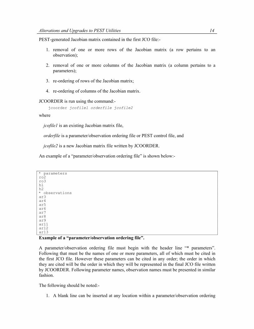
An example of a “parameter/observation ordering file” is shown below:-

* parameters ro2 ro3 h1 h2 * observations ar3 ar4 ar5 ar6 ar7 ar8 ar9 ar11 ar12 ar13

Example of a “parameter/observation ordering file”.

A parameter/observation ordering file must begin with the header line “* parameters”. Following that must be the names of one or more parameters, all of which must be cited in the first JCO file. However these parameters can be cited in any order; the order in which they are cited will be the order in which they will be represented in the final JCO file written by JCOORDER. Following parameter names, observation names must be presented in similar fashion.


1. A blank line can be inserted at any location within a parameter/observation ordering


file.

2. Any line beginning with the “#” character is ignored. Thus a comment can follow such a character.

3. Parameters and/or observations cited in the first JCO file can be omitted from the parameter/observation ordering file. These parameters/observations will then be omitted from the JCO file written by JCOORDER.

As an alternative to reading a parameter/observation ordering file, JCOORDER can read a PEST control file. It will recognise the fact that a PEST control file is supplied through the extension “.pst” supplied with this file on the JCOORDER command line. Ordering of parameters and observations will then be the same as that in the nominated PEST control file. The following should be noted:-

1. Tied and fixed parameters in the PEST control file are ignored.

2. Prior information in the PEST control file is ignored (however if prior information is detected in the PEST control file, JCOORDER asks the reader to confirm that it is alright to ignore it).

3. Parameters/observations occurring in the JCO file can be omitted from the PEST control file. However extra parameters and/or observations cannot appear in the PEST control file.

Use of JCOORDER can be a necessary adjunct to the use of JCOPCAT in preparation for SVD-assisted parameter estimation where PEST runs are undertaken for the purpose of obtaining sensitivities for subsets of base parameters. The Jacobian matrices produced through this process will need to be concatenated into one big base Jacobian matrix. However it is quite possible that they will include different items of prior information; prior information is ignored by JCO2JCO and SVDAPREP when preparing for an SVD-assisted PEST run. Hence before parameter-concatenation of Jacobian sub-matrix JCO files using JCOPCAT, it will be necessary to remove the rows of these files which pertain to prior information, so that these matrices are compatible. Column re-ordering may also be necessary.

The easiest way to build a parameter/observation ordering file is to first run JCO2MAT on the Jacobian matrix requiring row/column removal and/or row/column re-ordering. Parameter and observation names are listed as column and row names respectively in this file. A little cutting and pasting with a text editor will soon result in a parameter/observation ordering file. Alternatively, a parameter/observation ordering file can be easily built from a PEST control file – perhaps the base PEST control file which the concatenated JCO file is being built to complement prior to running SVDAPREP.


4. Model Predictive Error Analysis 4.1 Concepts

4.1.1 General

As is explained in Moore and Doherty (2005), the parameter error covariance matrix C(p-p) of a calibrated model can be calculated using the formula:-

C(p -p) = (I - R)C(p)(I - R)t + GC(ε)Gt (4.1)

where:-

p represents “true” model parameters (which we never know);

p represents calibrated model parameters;

C(p) represents the covariance matrix of true parameters (often described by a variogram);

C(ε) represent the covariance matrix of measurement noise (mostly assumed to be a diagonal matrix);

R is the so-called “resolution matrix”; and

G is the matrix through which estimated parameter values (i.e. the elements of p) are calculated from measurements, referred to herein as the “parameter solution matrix”, or more simply as the G matrix.

Let s be a model prediction whose sensitivities to model parameters are encapsulated in the vector y. For a linear model, the “true” value of a model prediction is given by:-

s = ytp (4.2a)

while its model-calculated counterpart is:-

s = ytp (4.2b)

Model predictive error (which is never known) is given by:-

s – s = yt(p-p) = yt(I – R)p - ytGε (4.3)

while model predictive error variance (i.e. the “variance of potential wrongness” of a model prediction) is given by:-

σ2s-s = yt(I – R)C(p)(I – R)ty + ytGC(ε)Gty (4.4)

A comprehensive document showing the derivation of these equations can be provided on


request. Note that while their derivation rests on an assumption of model linearity, they are nevertheless correct to a good approximation when applied to many non-linear models – good enough, for example, to be used in the ranking of different data acquisition strategies in terms of their comparative ability to reduce the potential wrongness of a key model prediction. Furthermore, their application can be extended to nonlinear analysis without too much difficulty; please contact the author for further details.

4.1.2 Calculation of the R and G Matrices

Formulas for R and G depend on the method used by PEST to solve the inverse problem. For an overdetermined system, for which the regularisation opportunities offered by truncated SVD, SVD-assist and Tikhonov schemes are not required, the resolution matrix R is I. However in many cases potentially unstable overdetermined problems are rescued from numerical instability by use of a high Marquardt lambda (which is a de-facto Tikhonov regularisation device). The Marquardt lambda is employed in the calculation of the R and G matrices in the utility software described below. However it must be noted that this is not a very good regularisation device, and in many cases can lead to loss of diagonal dominance of the resolution matrix. Hence, whether using one of the specialist regularisation devices offered by PEST, or not, attempts should be made to keep the Marquardt lambda low (or even zero, as is suggested when using truncated SVD as a regularisation mechanism).

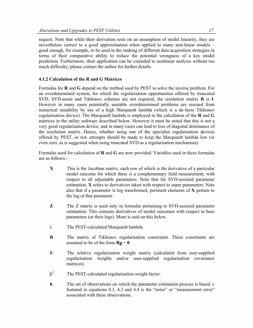
Formulas used for calculation of R and G are now provided. Variables used in these formulas are as follows:-

X This is the Jacobian matrix, each row of which is the derivative of a particular model outcome for which there is a complementary field measurement, with respect to all adjustable parameters. Note that for SVD-assisted parameter estimation, X refers to derivatives taken with respect to super parameters. Note also that if a parameter is log transformed, pertinent elements of X pertain to the log of that parameter.

Z The Z matrix is used only in formulas pertaining to SVD-assisted parameter estimation. This contains derivatives of model outcomes with respect to base parameters (or their logs). More is said on this below.

λ The PEST-calculated Marquardt lambda.

R The matrix of Tikhonov regularisation constraints. These constraints are assumed to be of the form Rp = 0.

S The relative regularisation weight matrix (calculated from user-supplied regularisation weights and/or user-supplied regularisation covariance matrices).

β2 The PEST-calculated regularisation weight factor.

h The set of observations on which the parameter estimation process is based. ε featured in equations 4.1, 4.3 and 4.4 is the “noise” or “measurement error” associated with these observations.


Q The measurement weight matrix (calculated from user-supplied measurement weights and user-supplied measurement covariance matrices).

V The matrix whose columns are orthogonal unit eigenvectors of XtQX as calculated through singular value decomposition undertaken either during every iteration of the parameter estimation process (when this is achieved through truncated SVD), or at the beginning of the parameter estimation process for determination of super parameters (if using SVD-assisted parameter estimation).

E A diagonal matrix whose elements are the eigenvalues of XtQX (arranged in decreasing order) determined through singular value decomposition.

V1 The first k columns of V, where k is the singular value truncation limit, or the number of super parameters employed in SVD-assisted parameter estimation.

E1 A diagonal matrix whose elements are the first k eigenvalues of XtQX.

The utility software described below through which R and G can be calculated, employs the X matrix corresponding to the best parameter set achieved through the parameter estimation process. This is stored in file case.jco which, like case.rsd (see below) and case.par (the parameter data file) is updated by PEST whenever an improved parameter set is obtained. The Z matrix, however, is not updated through the parameter estimation process. The utility software documented below provides the user with the option of using the Z matrix computed during the pre-SVD-assist base parameter sensitivity run, or of using a new Z matrix computed using optimised parameters; if possible, it is better to use the latter.

Formulas through which R and G are calculated are now presented.

Overdetermined parameter estimation.

R = (XtQX + λI)-1XtQX (4.5a)

G = (XtQX + λI)-1XtQ (4.5b)

Tikhonov Regularisation

R = (XtQX + β2RtSR + λI)-1XtQX (4.6a)

G = (XtQX + β2RtSR + λI)-1XtQ (4.6b)

Singular Value Decomposition with Zero Marquardt Lambda

R = V1V1t (4.7a)

G = V1E1-1V1

tXtQ (4.7b)


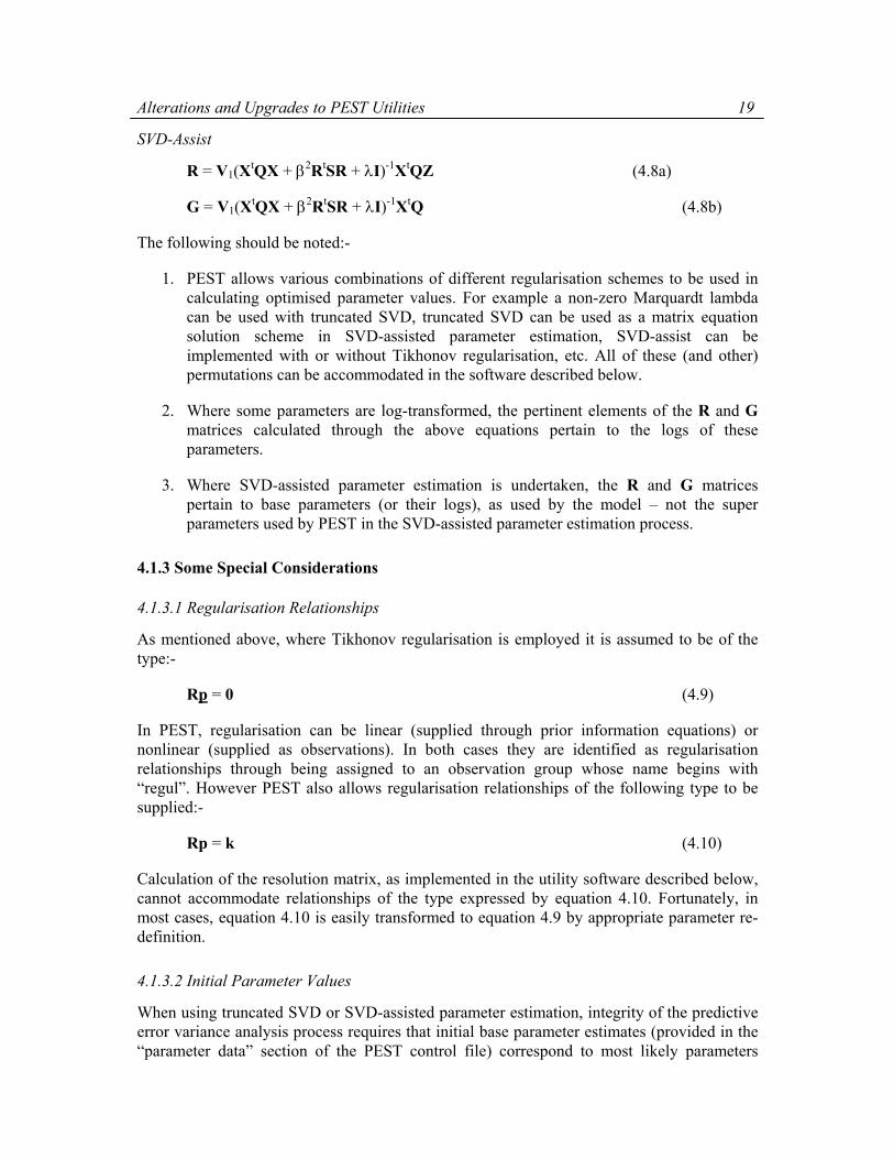
SVD-Assist

R = V1(XtQX + β2RtSR + λI)-1XtQZ (4.8a)

G = V1(XtQX + β2RtSR + λI)-1XtQ (4.8b)


1. PEST allows various combinations of different regularisation schemes to be used in calculating optimised parameter values. For example a non-zero Marquardt lambda can be used with truncated SVD, truncated SVD can be used as a matrix equation solution scheme in SVD-assisted parameter estimation, SVD-assist can be implemented with or without Tikhonov regularisation, etc. All of these (and other) permutations can be accommodated in the software described below.

2. Where some parameters are log-transformed, the pertinent elements of the R and G matrices calculated through the above equations pertain to the logs of these parameters.

3. Where SVD-assisted parameter estimation is undertaken, the R and G matrices pertain to base parameters (or their logs), as used by the model – not the super parameters used by PEST in the SVD-assisted parameter estimation process.

4.1.3 Some Special Considerations

4.1.3.1 Regularisation Relationships

As mentioned above, where Tikhonov regularisation is employed it is assumed to be of the type:-

Rp = 0 (4.9)

In PEST, regularisation can be linear (supplied through prior information equations) or nonlinear (supplied as observations). In both cases they are identified as regularisation relationships through being assigned to an observation group whose name begins with “regul”. However PEST also allows regularisation relationships of the following type to be supplied:-

Rp = k (4.10)

Calculation of the resolution matrix, as implemented in the utility software described below, cannot accommodate relationships of the type expressed by equation 4.10. Fortunately, in most cases, equation 4.10 is easily transformed to equation 4.9 by appropriate parameter re-definition.

4.1.3.2 Initial Parameter Values

When using truncated SVD or SVD-assisted parameter estimation, integrity of the predictive error variance analysis process requires that initial base parameter estimates (provided in the “parameter data” section of the PEST control file) correspond to most likely parameters


according to a user’s conception of parameter likelihood based on the current modelling context and the characteristics of the modelled area.

4.1.3.3 The Z Matrix

As mentioned above, the Z matrix appearing in equation 4.8a provides the sensitivities of model outputs for which there are corresponding field measurements to base parameters. In SVD-assisted parameter estimation these can far outnumber super parameters, and computation of the Z matrix can therefore be costly. Nevertheless, as described in the PEST manual, this matrix must be calculated (based on initial parameter values) prior to the undertaking of SVD-assisted parameter estimation, and so should be available for calculation of the resolution matrix upon completion of the SVD-assisted parameter estimation process. A better matrix to use in (4.8a) however is a Z matrix calculated on the basis of optimised parameter values. Thus, after an SVD-assisted PEST run is complete, the PARREP utility can be used to build a new base PEST control file using optimised base parameter values. NOPTMAX can be set to “-1” in this new file so that when PEST is run it terminates execution as soon as the Jacobian matrix is filled. The resulting “JCO” file will then hold the Z matrix of sensitivities, calculated on the basis of optimized parameter values.

4.2 Alterations to PEST

4.2.1 The IRES Variable

In addition to its normal suite of output files, PEST now writes a “resolution data file” named case.rsd where case is the filename base of the current PEST control file. If desired, writing of this file can be enabled or suppressed using a new variable (named “IRES”) which should be supplied following the IEIG variable on the tenth line of the PEST control file. If IREG is omitted, its value is assumed to be “1” if PEST is run in regularisation mode and/or if PEST’s SVD or SVD-assist functionality is activated, thus ensuring that file case.rsd is written. However if IRES is set to zero, writing of case.rsd is suppressed. (It is automatically set to zero if PEST is run in predictive analysis mode.) Figure 4.1 shows the structure of the “control data” section of the PEST control file with the IRES variable included.

* control data RSTFLE PESTMODE NPAR NOBS NPARGP NPRIOR NOBSGP NTPLFLE NINSFLE PRECIS DPOINT NUMCOM JACFILE MESSFILE RLAMBDA1 RLAMFAC PHIRATSUF PHIREDLAM NUMLAM RELPARMAX FACPARMAX FACORIG PHIREDSWH NOPTMAX PHIREDSTP NPHISTP NPHINORED RELPARSTP NRELPAR ICOV ICOR IEIG IRES

Figure 4.1 Structure of the “control data” section of a PEST control file.

4.2.2 The “Resolution Data File”

The resolution data file case.rsd is a binary file whose contents cannot be read by the user. Instead it is used by the RESPROC utility described below for calculation of the R and G


matrices of equations 4.5 to 4.8.

Upon commencement of execution, PEST deletes an existing resolution data file having the same filename base as that of the current PEST control file if such a file is found. This eliminates the possibility that an old file will be confused for a new one if PEST did not run long enough to produce this file, or if IRES was inadvertently set to zero.

PEST updates the resolution data file many times during the course of the parameter estimation process such that data contained within it always pertains to the best parameters achieved so far during that process; it is thus overwritten whenever the estimated parameter set is improved.

4.3 RESPROC

4.3.1 General

RESPROC stands for “RESolution data post PROCessor”. It is run after completion of a PEST run; normally PEST will have been run in regularisation mode, or with SVDMODE set to 1, or with its SVD-assist functionality activated, or a combination of these. However RESPROC can also provide useful results after a PEST run in which traditional parameter estimation was implemented without the aid of any regularisation device (except the Marquardt lambda). In all cases a “resolution data file” (named case.rsd where case is the filename base of the PEST control file) must have been produced on that PEST run.

RESPROC’s task is to write a file containing both the R and G matrices pertaining to the previous PEST run, which can then be used by other utility programs for calculation of parameter and predictive error variances. In order to save disk space this, too, is a binary file; however the R and G matrices can be rewritten in ASCII form if desired using the RESWRIT utility described below.

4.3.2 What RESPROC Does

RESPROC reads the following files, all associated with an existing PEST dataset characterised by the case filename base:-

1. the PEST control file (named case.pst);

2. the resolution data file (named case.rsd);

3. the Jacobian matrix file (named case.jco).

(Note that at any stage of the parameter estimation process the contents of the latter two files pertain to the best parameters achieved at that stage of the process. )

If the previous PEST run implemented SVD-assisted parameter estimation, the following files are also read by RESPROC:-

1. the base pest control file in which base parameters are defined (named bcase.pst);


2. the base Jacobian matrix file in which base parameter sensitivities are recorded (named bcase.jco);

3. Optionally, an updated JCO file in which base sensitivities are recorded for optimised base parameter values.

Where many parameters and observations are involved in the parameter estimation process, RESPROC may take a while to run, for the matrices that must be manipulated in the formulation of R and G can be large. Fortunately, it need only be run once, for these matrices, once calculated, can then be used for computation of the error variance of a variety of model predictions.

As presently programmed there is a slight restriction on the use of RESPROC, which it is hoped will not limit its usefulness too much. RESPROC insists that no covariance matrix in lieu of observation weights be used for observation groups pertaining to measurements; however it will accept the use of a covariance matrix for an observation group containing regularisation information.

4.3.3 Running RESPROC

RESPROC is run using the command:- resproc case outfile

where :-

case is the filename base of the PEST control file pertaining to a completed PEST run, and

outfile is the name of the RESPROC output file containing the R and G matrices (referred to herein as a “binary resolution matrix file”).

When supplying case on the RESPROC command line, the “.pst” extension can be omitted; if so, RESPROC will supply this extension automatically. outfile, however, must have its extension supplied; if it is omitted, RESPROC will assume that this file has no extension.

As it executes, RESPROC writes its current activities to the screen. As discussed above, these activities involve manipulation of possibly large matrices. They also involves matrix inversion and possibly singular value decomposition (which will need to be undertaken twice if the previous parameter estimation was SVD-assisted and if truncated SVD was employed for estimation of super parameters). Hence, as mentioned above, execution of RESPROC may take a while. When it has completed calculation of R and G, RESPROC stores them in its output binary resolution matrix file, records this fact to the screen, and ceases execution.

4.3.4 SVD-Assisted Parameter Estimation

Where the previous PEST run implemented SVD-assisted parameter estimation, RESPROC prompts the user for some extra information as follows:- Select option for obtaining base parameter sensitivities:- enter "1" to use those in base Jacobian matrix file bcase.jco enter "2" to read from another JCO file

Alterations and Upgrades to PEST Utilities 23Enter your choice:

If your response to the above prompt is “2”, RESPROC asks for the name of a JCO file. This file must cite the same parameters and observations (including prior information) as the base parameter PEST control file used in setup of the SVD-assisted run. This will be automatically ensured if the following steps are taken for preparation and implementation of SVD-assisted parameter estimation, and subsequent postprocessing:-

1. A PEST case is set up involving base parameters, and optional Tikhonov regularisation constraints. Let us suppose that the PEST control file for this case is named bcase.pst.

2. Base parameter sensitivities are calculated for this base case. These will be stored in the base Jacobian matrix file bcase.jco.

3. A super parameter dataset is constructed using SVDAPREP; let the new PEST control file be named case.pst.

4. PEST is run; after this run is complete, optimised base parameters reside in file bcase.bpa.

5. PARREP is run to build a new base PEST control file, bcase1.pst in which optimized parameter values are employed as parameter initial values. The command is:- parrep bcase.bpa bcase.pst bcase1.pst

6. NOPTMAX is set to “-1” in bcase1.pst. Thus it calculates the Jacobian matrix (the Z matrix of equation 4.8a), and then terminates execution. This matrix is stored in file bcase1.jco.

7. When RESPROC is run, a “2” is supplied in response to the above prompt. bcase1.jco is then supplied as the name of the alternative base Jacobian matrix file.

Limited experience to date suggests that use of a Z matrix calculated on the basis of optimized base parameter values results in a better resolution matrix than use of the original Z matrix contained in file bcase.jco which was used for definition of super parameters).

4.4 RESWRIT

4.4.1 General

The R and G matrices written by RESPROC are not readable by the user. If it is desired that these matrices be subject to inspection and/or plotting, they should be converted to ASCII format. RESWRIT accomplishes this task.

4.4.2 Running RESWRIT

RESWRIT is run using the command:- reswrit resprocfile matfile1 matfile2

where


resprocfile is the name of an unformatted RESPROC output file;

matfile1 is a “matrix file” to which the resolution matrix will be written; and

matfile2 is a “matrix file” to which the “G” matrix will be written.

Note that an extension must be provided for each of these files, for RESWRIT employs no default extensions.

4.4.3 Format of Matrix Files

A matrix file holding a matrix with three rows and four columns is illustrated in Figure 4.2. 3 4 2 3.4423 23.323 2.3232 1.3232 5.4231 3.3124 4.4331 3.4442 7.4233 5.4432 7.5362 8.4232 * row names apar1 apar2 apar3 * column names aobs1 aobs2 aobs3 aobs4 Figure 4.2 An example of a matrix file.

The first line of a matrix file contains 3 integers. The first two indicate the number of rows and number of columns in the following matrix. The next integer (named ICODE) is a code, the role of which will be discussed shortly.

Following the header line is the matrix itself, in which entries are space-separated and wrapped to the next line if appropriate.

Then, if ICODE is set to 2, follows the string “* row names”. Following that are NROW names (of 20 characters or less in length), containing the names associated with rows of the matrix. NCOL column names follow in a similar format.

For a square matrix ICODE can be set to “1”. This indicates that rows and columns are associated with the same names (as is the case for a resolution matrix). In this case the string “* row and column names” follows the matrix, and the pertinent names are listed on the NROW lines following that.

A special ICODE value is reserved for diagonal matrices. If NCOL is equal to NROW, then ICODE may be set to “-1”. In this case only the diagonal elements of the matrix need to be presented following the integer header line; these should be listed one to a line as illustrated in Figure 4.3. Following that should be the string “* row and column names” (for if ICODE is set to “-1” it is assumed that these are the same), followed by the names themselves.


5 5 -1 4.5 4.5 2.4 7.53 5.32 * row and column names par1 par2 par3 par4 par5

Figure 4.3 A matrix file containing a diagonal matrix.

4.5 PARAMERR

4.5.1 General

PARAMERR’s task is to construct the “parameter error covariance matrix” C(p-p) of equation (4.1). It stores the two terms on the right side of equation 4.1 in separate files. This saves the user from having to re-compute both of these terms if an input required by only one of them (for example C(p) or C(ε)) is altered. It also allows the user to quantify the individual contribution to overall predictive error variance made by “uncaptured system heterogeneity” on the one hand (the first term), and measurement error on the other (the second term). The first diminishes as the level of fit between model outputs and field measurements increases, while the second term grows as better model-to-measurement fits are obtained; as Moore and Doherty (2005) point out, the optimal level of model-to-measurement misfit for any particular parameter estimation problem is that which minimises the variance of one or a number of key model predictions.

4.5.2 Uncertainty Files

4.5.2.1 Concepts

Calculation of C(p-p) requires that the user provide the covariance matrices C(p) and C(ε). These must each be specified through an “uncertainty file”, an example of which is shown in Figure 4.4. # An example of an uncertainty file START STANDARD_DEVIATION std_multiplier 3.0 ro9 1.0 ro10 1.0 ro4 1.0 END STANDARD_DEVIATION START COVARIANCE_MATRIX file "mat.dat" variance_multiplier 1e-2 END COVARIANCE_MATRIX START PEST_CONTROL_FILE file "te st.pst"


variance_multiplier 2.0e2 END PEST_CONTROL_FILE

Figure 4.4. Example of an uncertainty file.

The purpose of an uncertainty file is to allow the user a number of different options for characterising the uncertainty of a group of entities comprising a vector quantity (for example p and ε). Three such options are presently available, viz. a list of individual entity standard deviations, a covariance file, and entity weights listed in the “observation data” section of a PEST control file. A single such option can be used to specify the entirety of a covariance matrix, or different mechanisms can be used to characterise different parts of the total covariance matrix.

An uncertainty file is subdivided into blocks. Each such block implements one of the mechanisms of uncertainty characterisation described above. An uncertainty file can have as many blocks as desired. However the following rules must be observed:-

1. Any one uncertainty file is used to characterize the uncertainty of either parameters or observations, but not both.

2. Parameters and observations cited in an uncertainty file, and the files cited therein, are matched by name to those featured in the current parameter estimation problem.

3. The uncertainty of an individual element of the overall p or ε vector can be characterised in only one way. Thus any particular element cannot be cited in the “observation data” section of a PEST control file cited in a particular uncertainty file if it is also cited in a standard_deviation block of that uncertainty file, or in a covariance matrix file cited in the COVARIANCE_MATRIX block of that same uncertainty file.

4. An uncertainty file, and files cited therein, can cite the names of parameters and observations that are not featured in the current parameter estimation problem; data pertaining to these surplus parameters and observations are simply ignored. However it must not omit any of the parameters or observations pertaining to the current parameter estimation problem.

5. If a parameter is log-transformed in the current parameter estimation problem, then specifications of variance, covariance or standard deviation provided in the uncertainty file must pertain to the log of the parameter. PARAMERR provides no checks for this, for it has no way of knowing the transformation status of a particular parameter; it is thus the user’s responsibility to ensure that this protocol is observed.

6. An uncertainty file used for the characterisation of C(p) cannot include a PEST_CONTROL_FILE block, for PARAMERR reads only the “observation data” section of a cited PEST control file.

7. As presently programmed, an uncertainty file used for characterisation of C(ε) must not include a COVARIANCE_MATRIX block, for PARAMERR assumes that measurement noise is uncorrelated.


Each block of an uncertainty file must begin with a START line and finish with an END line as illustrated in Figure 4.4; in both cases the type of block must be correctly characterised following the START and END designators. Within each block, data entry must follow the keyword protocol concept. Thus each line must comprise a keyword, followed by the value (numerical or text) associated with that keyword. Filenames must be surrounded by quotes if they contain spaces. With one exception (the std_multiplier keyword in the STANDARD_DEVIATION block), keywords within a block can be supplied in any order; some can be omitted if desired. Keywords and block names are case insensitive.

Blank lines can appear anywhere within an uncertainty file. So too can comment lines; these are recognised through the fact that their first character is “#”.

Each of the blocks appearing in an uncertainty file is now discussed in detail.

4.6.2.2 The STANDARD_DEVIATION Block

In a STANDARD_DEVIATION block, entity names (individual parameters or observations) are listed one to a line followed by their standard deviations. As stated above, if a parameter is log-transformed in the parameter estimation process, then this standard deviation should pertain to the log (to base 10) of the parameter. Parameters/observations can be supplied in any order. Optionally a std_multiplier keyword can be supplied in the STANDARD_DEVIATION block; if so, it must be the first item in the block. All standard deviations supplied on ensuing lines are multiplied by this factor (the default value of which is 1.0).

Parameters/observations cited in a STANDARD_DEVIATION block are assumed to be uncorrelated with other parameters/observations. Thus off-diagonal elements of C(p) or C(ε) corresponding to these items are zero. Pertinent diagonal elements of C(p) and C(ε) are calculated by squaring the standard deviation (after multiplication by the std_multiplier).

4.5.2.3 The PEST_CONTROL_FILE Block

Only two keywords are permitted in this block, these being the file and variance_multiplier keyords; the latter is optional, the default value being 1.0.

The name of a PEST control file should follow the file keyword. PARAMERR reads the “observation data” section of this file. For any particular observation cited in this section that is also featured in the current parameter estimation problem, PARAMERR calculates its variance from the weight w cited in the PEST control file as (1/w)2. This variance is then multiplied by the variance_multiplier before insertion into the appropriate diagonal element of C(ε). Corresponding off diagonal elements of C(ε) are assumed to be zero.

4.5.2.3 The COVARIANCE_MATRIX Block

Where one or more covariance matrices are supplied for subgroups of p which show intra-parameter correlation, these matrices are included in the larger C(p) matrix calculated by PARAMERR (together with variances calculated from parameter standard deviations supplied in one or more standard_deviation blocks). Optionally, all elements of such a user-supplied covariance matrix can be multiplied by a factor, this factor (for which the default


value is 1.0) being supplied following the variance_multiplier keyword.

The format of a covariance matrix file must be identical to that depicted in Figures 4.2and 4.3. In particular, the first line of this file must include 3 integers, the first two of which (specifying the number of rows and columns in the matrix) must be identical. The third integer must be “1” or “-1”. The matrix itself must follow this integer header line; elements within this matrix must be space-delimited; rows can be wrapped onto consecutive lines. This matrix must be followed by the string “row and column names”. Following this must be the names of the parameters to which the matrix pertains.

The following must be noted.

1. A covariance matrix must be positive definite.

2. The order of rows and columns of the covariance matrix (which corresponds to the order of parameters represented by this matrix as listed below the “row and column names” header) is arbitrary. PARAMERR will re-arrange these rows so that they correspond to the order of adjustable parameters supplied in the PEST control file on which the current parameter estimation problem is based.

3. A user-supplied covariance matrix need not contain all of the parameters pertaining to the current parameter estimation problem, for it need contain only a subset of these. (Other parameters can be cited in other covariance matrix files and/or one or more STANDARD_DEVIATION blocks supplied in the same uncertainty file.) However it must not contain any parameters which do NOT pertain to the current parameter estimation problem (unless none of its parameters pertain to the current parameter estimation problem, in which case the matrix is ignored).

4. If a parameter is log-transformed, the variance and covariances pertaining to that parameter as supplied in a covariance matrix file must in fact pertain to the log of that parameter.

4.5.3 Using PARAMERR

PARAMERR receives information from keyboard input supplied by the user in response to a set of prompts. (It requires too much information to be supplied through command-line arguments.)

Upon commencement of execution, PARAMERR prompts:- Enter name of RESPROC output file:

in response to which the name of the RESPROC-generated unformatted resolution matrix file should be supplied (this file also contains the G matrix). Next it asks:- Options are as follows:- to compute (I-R)C(p)(I-R)' - enter 1 to compute GC(e)G' - enter 2 to compute both - enter 3 Enter your choice:.

As mentioned above, there will be occasions when only one of the two terms on the right side of equation 4.1 will require computation. However if both are required, enter 3. If this is


done, PARAMERR’s next prompts will be:- Enter name of parameter uncertainty file: Enter name for covariance matrix output file: Enter name of observation uncertainty file: Enter name for covariance matrix output file:

As discussed above, the uncertainty file in each case must be prepared by the user. The covariance matrix output file written by PARAMERR in each case is the respective term of equation (4.1), that is (I - R)C(p)(I - R)t in the first case and GC(ε)Gt in the second case. These are written in standard matrix file format, following the protocol shown in Figures 4.2 and 4.3. Each of these matrices is square with dimensions n × n where n is the number of adjustable parameters pertaining to the current parameter estimation problem.

4.6 PREDERR

4.6.1 General

PREDERR is similar in many respects to PARAMERR. Like PARAMERR it reads a parameter uncertainty file and an observation uncertainty file; see the documentation of PARAMERR for the format of these files. However rather than calculating and storing the two components of C(p–p), it directly calculates the error variance of a user-specified prediction. Thus calculation of C(p–p) is bypassed. This can result in enormous savings in calculation of predictive error variance. Thus unless calculation of C(p-p) is specifically required for a certain application, use of PREDERR is preferred over use of PARAMERR followed by JROW2VEC and MATQUAD for the calculation of the error variance of a certain prediction.

4.6.2 Using PREDERR

Many of PREDERR’s prompts are similar to those of PARAMERR. However, unlike PARAMERR (but like JROW2MAT and JROW2VEC), PREDERR requires the name of a Jacobian matrix file, as well as the name of an observation for which parameter sensitivities are recorded in this file. This “observation” is treated as a “prediction” for the purpose of error variance calculation as undertaken by PREDERR using equation 4.4. That is, the parameter sensitivities extracted from the user-specified Jacobian matrix constitute the y vector of this equation.

PREDERR’s screen display, including its prompts, are as follows; typical responses are shown highlighted. Enter name of RESPROC output file: modela.rpo Enter name of parameter uncertainty file: param1.unc Enter name of observation uncertainty file: observ1.unc Enter name of Jacobian matrix file: model1.jco Enter name of prediction featured in this file: ptime - reading RESPROC output file modela.rpo... - file modela.rpo read ok.

Alterations and Upgrades to PEST Utilities 30- reading Jacobian matrix file model1.jco... - Jacobian matrix file model1.jco read ok. - reading parameter uncertainty data... - parameter uncertainty data read ok. - calculating I-R contribution to predictive error variance... - I-R term calculated ok. - reading observation uncertainty data... - reading PEST control file temp.pst... - file temp.pst read ok. - observation uncertainty data read ok. - calculating G contribution to predictive error variance... - G term calculated ok.


1. The Jacobian matrix file will have been written by PEST. It is an unformatted file with the name case.jco where case is the filename base of the corresponding PEST control file.

2. The cited Jacobian matrix file must contain an observation named as the “prediction” in the pertinent PREDERR prompt. Many more observations than this can be cited in the Jacobian matrix file; all others are ignored.

3. Each parameter cited in the RESPROC output file must also be cited in the Jacobian file. If more parameters than this are cited in the Jacobian matrix file, they are ignored. If fewer parameters are cited, PREDERR ceases execution with an appropriate error message. Parameters need not be arranged in the same order in the Jacobian matrix file as they are in the RESPROC output file (and hence in the PEST control file on which the RESPROC output file is based).

PREDERR quickly calculates the contribution to predictive error variance made by both terms of equation 4.4 (which it refers to as the “I-R term” and the “G term”). It writes the outcomes of its calculations to the screen, an example of which is depicted below. *********** COMPONENTS OF PREDICTIVE ERROR VARIANCE *********** I-R component of predictive error variance = 2881711. G component of predictive error variance = 5342.439 Total predictive error variance = 2887054. Predictive error standard deviation = 1699.133 ****************************************************************

4.7 PREDVAR1

4.7.1 General

PREDVAR1 analyses “notional predictive error variance” without requiring that a model be actually calibrated to do so. Equation 4.4 is employed on the assumption that the notional calibration exercise is completed using singular value decomposition (SVD).

PREDVAR1 can be extremely useful in achieving at least the following objectives.


1. Before a model is even calibrated, a rapid assessment can be made of the reduction in predictive variance that can be achieved through the calibration process, given the number and type of measurements comprising the calibration dataset, the noise C(ε) associated with these measurements, and the inherent variability C(p) of model parameters as a result of environmental system complexity and/or heterogneity. By comparing post-calibration predictive variance with pre-calibration predictive variance calculated as

s = ytC(p)y (4.11)

a rapid assessment can be made of the worth of undertaking a possibly expensive calibration exercise before that exercise is actually embarked upon.

2. Because the calibration exercise simulated by PREDVAR1 is notional rather then actual, the reduction in uncertainty accrued through including one or a number of hypothetical extra observations in the calibration dataset can be assessed. This can form a sound scientific basis of optimisation of data acquisition, based on the premise that the worth of acquiring a certain type of data over that or acquiring another is greater if its acquisition results in a greater reduction in predictive error variance. Furthermore, because equation 4.4 is based on a full characterization of uncertainty (including the effects of heterogeneity which is beyond the ability of the calibration process to capture), this method of assessing the worth of extra data is superior to similar statistics based on over-determined estimation of over-simplified models which, under most circumstances of environmental model calibration, are almost meaningless.

3. Similarly, by varying the terms of C(p) in accordance with an improvement in direct knowledge of system properties that may be gained through direct system measurement, an assessment of the worth of these measurements in reducing the uncertainties of one or more predictions can be made. Various data acquisition strategies of this type can then be ranked, and or these strategies can be compared with the beneifits of acquiring extra information on system states (see the above point).

4. By setting certain components, or groups of components, of C(p) to zero and by employing equation 4.4 and/or 4.11 in conjunction with this revised C(p), the contribution to the uncertainty of a specific model prediction made by different parameter types can be estimated. Where knowledge of the values of those parameter types cannot be enhanced by direct measurement, this may allow the user to determine the “irreducible level of uncertainty” associated with key model predictions.

5. By re-calculating error variance using equation 4.4, for different numbers of singular values prior to truncation of the SVD process, the minimum in the curve of number of singular values versus model predictive error variance can be ascertained; see Moore and Doherty (2005). This can serve as a useful guide to the number of super parameters to employ in SVD-assisted parameter estimation.

As mentioned above, PREDVAR1 calculates predictive error variance on the assumption that


regularisation of the notional calibration exercise is implemented using truncated SVD. Thus equations 4.7a and 4.7b are thus employed in the calculation of R and G. It is further assumed that the user supplies a set of measurement weights for this calibration exercise that satisfies the equation:-

Q = σr2C(ε) (4.12)

where Q is the weight matrix. Use of this relationship further simplifies (and expedites) calculation of σ2

s-s using equation 4.4. Note that one or more measurement covariance matrices can be used instead of weights as discussed below.

4.7.3 Using PREDVAR1

PREDVAR1 requires too many inputs for these to be supplied through its command line. So it prompts the user for information, which must be supplied in response to these prompts. PREDVAR1 commences execution with the prompt:- Enter name of PEST control file:

Supply the name of a PEST control file. It is assumed that a complementary Jacobian matrix file (“JCO file”) is available for this PEST control file. Thus it is assumed that PEST has been run for one iteration (or that it NOPTMAX has been set to -1 on its previous run) so that derivatives have been calculated for all model outputs with respect to all adjustable model parameters. (Predictive sensitivities may also have been calculated – see below).

Next PREDVAR1 prompts: Enter observation reference variance:

PREDVAR1 computes C(ε) of equation 4.4 by assuming that weights contained in the PEST control file are proportional to the inverse of the standard deviations of the observations to which they are assigned. It is assumed that the proportionality constant is the same for all weights, and is equal to the square root of the reference variance depicted equation 4.12. That is, weights are assumed to comprise the inverse of the diagonal of the Q matrix of equation 4.12. If desired the PEST control file can feature one of more observation covariance matrices as well, these being used instead of weights for one or more observation groups. The same reference variance must apply to these as well.

PREDVAR1 next prompts for the name of a parameter uncertainty file. The prompt is:- Enter name of parameter uncertainty file:

The contents of this file define C(p); see documentation of program PARAMERR for details. The uncertainties associated with elements, or groups of elements, of the parameter vector p can be defined in in the parameter uncertainty file using standard deviations or covariance submatrices (possibly based on geostatistical characterizations of the subsurface). The following should be noted.

• If a parameter is log-transformed in the PEST control file, the elements of C(p) associated with that parameter must pertain to the log of that parameter.

• As is the protocol for a parameter uncertainty file, this file can contain information pertaining to more parameters than those which are demarcated as adjustable in the


PEST control file. Unused parameters are simply ignored.

• If one parameter is tied to another parameter in the PEST control file, then the parent parameter is in fact a “composite parameter”. Its statistical properties as supplied in C(p) should reflect this.

Next PREDVAR1 prompts:- Enter name of predictive sensitivity matrix file:

This file must contain a single column matrix (in matrix file format) which contains the sensitivity of a prediction of interest to every adjustable parameter cited in the PEST control file. That is, it must contain the vector y of equation 4.4. The following should be noted.

• If a parameter is log transformed in the PEST control file, then parameter sensitivities contained in y must pertain to the log of the parameter.

• If a parameter is tied to another parameter in the PEST control file, then the sensitivity with respect to the parent parameter as contained in y must reflect the fact that it is parent to another parameter.

• Parameters do not need to be arranged in the same order in the predictive sensitivity matrix file as they are in the PEST control file. PREDVAR1 links them by name in that file, and re-arranges them if necessary. Similarly, if the predictive sensitivity matrix file cites more parameters than are adjustable in the PEST control file, then the excess parameters are simply ignored.

The easiest way to make a predictive sensitivity matrix file is as follows:

• When PEST is run in order to calculate observation sensitivities, design the model to run in such a way that it makes one or more predictions as well as calculating outputs that correspond to observations listed in the PEST control file. This may require that the model be run not once, but twice, based on different inputs, through a batch file serving as the model.

• List these predictions in the PEST control file as additional “observations”. However give them a weight of zero.

• If this is done, the JCO file produced as an outcome of the PEST run will contain the sensitivities of these predictions to all adjustable parameters. A predictive sensitivity file can be constructed for each such prediction using the JROW2VEC utility.

Next PREDVAR1 issues a series of prompts as follows:- Enter no. of singular values before truncation [<Enter> if no more]:

Enter a number between (and including) zero and the number of adjustable parameters employed in the simulation. Be aware, however, that if there are more adjustable parameters than observations, the number of non-zero singular values will be only as large as the number of observations. So do not enter a number higher than this. PREDVAR1 will inform you if this number is too high as a result of a zero singular value; in fact it will cease execution with


an error message. So when entering singular values in response to the above series of prompts it is best to supply them in increasing order.

If truncation takes place at zero singular values, this is equivalent to not calibrating the model at all. Hence predictive error variance is calculated using equation 4.10. As the number of singular values prior to truncation increases, the first term of equation 4.10 will normally fall. In fact it will fall monotonically if C(p) is the equal to σ2

pI where I is the identity matrix. There may be interruptions in the fall (and sometimes considerable rises with singular value – indicating that calibration can actually increase the error variance of a prediction unless carefully undertaken) if C(p) has variances of very different magnitude, and/or indicates a high level of parameter correlations. The former problem can be rectified by appropriate parameter scaling; this should be done as a matter of course when calibrating a model in order to prevent this problem.

The second term in equation 4.10 should rise as the location of singular value truncation increases. At some number of singular values there is normally an optimum, where predictive variance is least.

PREDVAR1 finally prompts for the names of its two output files:- Enter name for predictive error variance output file: Enter name for SVD results output file:

The first file lists the contributions to predictive variance made by the first and second terms of equation 4.10 for each requested singular value. It also lists the total predictive error variance, together with the predictive standard deviation (square root of this). If singular values are arranged in increasing order, this file can serve as an input to a plotting/graphing program. The second file is similar to that produced by PEST with implementing singular value decomposition as an inversion device. It lists singular values and respective eigenvalues of XtQX, calculated as an outcome of the SVD process.

It is important to note that if the PEST control file employed by PREDVAR1 instructs PEST to run in regularisation mode, regularisation observations and prior information equations are ignored in formulating X and hence in computation of predictive error variance. Thus it is assumed that the only type or regularisation undertaken is that pertaining to truncated SVD, with the truncation limit set at one or a number of singular values according to input data supplied by the user.

4.8 OBSREP

4.8.1 General

OBSREP does for observations what PARREP does for parameters. OBSREP reads optimised model outputs corresponding to observations and prior information from a “residuals file” produced as an outcome of a previous PEST runs. It then substitutes these values for “observed values” in the PEST control file. (It should be obvious from this that if both PARREP and OBSREP are run after completion of a PEST run, the objective function should be zero.)


4.8.2 Running OBSREP

OBSREP is run using the command:- obsrep resfile pestfile1 pestfile2

where

resfile is the name of a “residuals file” written by PEST (extension “.res”),

pestfile1 is the name of an existing PEST control file, and

pestfile2 is the name of the new PEST control file to be written by OBSREP.

In most cases the residuals file resfile will have been produced by PEST on the basis of a run undertaken using pestfile1 as the PEST control file. However this does not have to be the case. OBSREP will work correctly as long as every observation and prior information equation cited in the pestfile1 PEST control file is also cited in resfile residuals file. If resfile cites other observations and/or prior information items, and/or these are listed in a different order in resfile from that prevailing in pestfile1, OBSREP will not object. However if any observations or prior information items cited in pestfile1 are missing from resfile, OBSREP will cease execution with an appropriate error message.

4.9 PCOV2MAT

4.9.1 General

The purpose of PCOV2MAT is to facilitate the calculation of model predictive error variance in over-determined inversion contexts; these are contexts where regularisation is not employed as part of the inversion process. In these circumstances parameter error variance/covariance is completely described by the parameter covariance matrix produced as an outcome of the parameter estimation process. This is because, under these circumstances, the resolution matrix R of equation 4.1 is in fact the identity matrix I. If the measurement weight matrix Q is proportional to the inverse of the measurement noise matrix C(ε), then at the end of the parameter estimation process this can be updated through multiplication by the reference variance σ2

r calculated from the minimized objective function Фmin as:-

σ2r = Фmin/(n-m) (4.11)

where n and m are the number of observations and parameters respectively featured in the parameter estimation process. Thus Q now becomes:

Q = σ2r C-1(ε) (4.12)

and the parameter error covariance matrix (or simply “parameter covariance matrix” under these over-determined circumstances) can be calculated as:-

C(p-p) = σ2r(XtQX)-1 (4.13)

The parameter error covariance matrix is recorded by PEST at the end of its run record file case.rec; it is also calculated intermittently by PEST and recorded in the matrix file case.mtt.


In both of these cases case is the filename base of the PEST control file on which the current parameter estimation exercise is based.

If a prediction has parameter sensitivities y, then the error variance of that prediction can be calculated as:-

σ2s-s = ytC(p-p)y (4.14)

4.9.2 Using PCOV2MAT

PCOVMAT is run using the command:- pcovmat pestfile matfile

where

pestfile is the name of a PEST run record file or matrix file containing a covariance matrix, and

matfile is the name of the matrix file to which the matrix will be written.


1. Only adjustable parameters are cited in a parameter covariance matrix; fixed or tied parameters are not cited.

2. It is preferable to use the parameter covariance matrix from a run record file over that recorded in a matrix file as the former is calculated using sensitivities pertaining to optimized parameters, whereas the covariance matrix recorded in the latter file is calculated on the basis of sensitivities pertaining to the latest PEST iteration.

3. A covariance matrix is not recorded in the matrix file unless the ICOV variable in the “control data” section of the PEST control file is set to 1.

Once the parameter error covariance matrix has been translated by PCOV2MAT to matrix file format, the error variance of a particular prediction can be calculated using equation 4.14 using the MATQUAD utility documented herein. Prediction sensitivities can be extracted from a Jacobian matrix file using the JROW2VEC or JROW2MAT utilities; in the latter case the MATTRANS utility must be used before MATQUAD is employed to calculate predictive error variance.

4.10 MATRIX MANIPULATION PROGRAMS

4.10.1 General

A series of matrix manipulation programs has been written to assist in carrying out uncertainty analysis in the post-processing of regularised PEST runs. These utilities have been provided in order to allow processing of a more general nature than that provided by specific uncertainty-prediction utilities. It is hoped that this provides the user with a certain degree of flexibility in accommodating the demands of their particular modelling


applications.

All of these utilities read and write “matrix files” whose format follows that described above, and exemplified in Figure 4.3.

4.10.2 JCO2MAT

JCO2MAT reads a PEST-produced Jacobian matrix file. It re-writes the matrix contained therein in the same matrix file format as that employed by other utility programs documented herein. The Jacobian matrix is then amenable to manipulation of various kinds as described in this manual.

JCO2MAT is runusing the command:- jco2mat jcofile matfile

where:-

jcofile is the name of a Jacobian matrix file, and

matfile is the name of the matrix file to which the Jacobian matrix is to be written.

4.10.3 JROW2MAT

JROW2MAT extracts a row of a Jacobian matrix from a PEST unformatted “Jacobian matrix file” and writes that row as a 1×NPAR matrix to a standard matrix file, where NPAR is the number of (adjustable) parameters featured in the Jacobian matrix file. Note that the expected extension for a Jacobian matrix file is “.jco”.

JROW2MAT is run using the command:- jrow2mat jcofile obsname matfile

where:-

jcofile is the name of a Jacobian matrix file,

obsname is the name of an observation or prior information item featured in that file, and

matfile is the name of the matrix file to which the 1×NPAR matrix is to be written.

JROW2MAT simply extracts the nominated row of the Jacobian matrix and re-writes that row in appropriate format. The “row name” of the row is that of the extracted observation or prior information equation, while “column names” are the names of parameters featured in the Jacobian matrix file.

The reader is reminded that a PEST unformatted Jacobian matrix file can be viewed in ASCII format using the JACWRIT utility.


4.10.4 JROW2VEC

JROW2VEC performs the same function as JROW2MAT followed by MATTRANS. That is, it extracts a user-nominated row from a Jacobian matrix. However instead of writing the extracted row in the form of a row matrix, it writes it as a column matrix. Thus, if desired, the extracted set of observation or predictive sensitivities are immediately useable by MATQUAD for evaluation of predictive error variance.

JROW2VEC is run using the command:- jrow2vec jcofile obsname matfile

where:-

jcofile is the name of a Jacobian matrix file,

obsname is the name of an observation or prior information item featured in that file, and

matfile is the name of the matrix file to which the NPAR×1 matrix is to be written.

4.10.5 MAT2SRF

MAT2SRF rewrites a matrix in SURFER grid file format. This is a particularly useful device for viewing the resolution matrix. A highly diagonally dominant resolution matrix indicates (as the name suggests) good “resolution” of parameters through the parameter estimation process. A “blurry” resolution matrix which is only mildly diagonally dominant indicates inability of the calibration process to capture parameterisation detail, this arising from inadequacies in the information content of the calibration dataset as an outcome of data scarcity, data noise, or both.

MAT2SRF can read any matrix file which adheres to the format illustrated in Figures 4.2 and 4.3.

MAT2SRF is run using the command:- mat2srf matfile gridfile [threshold]

where

matfile is the name of a matrix file;

gridfile is the name of a SURFER grid file; and

threshold is a blanking threshold.

Upon commencement of execution, MAT2SRF reads the matrix contained in the matrix file. It then rewrites the matrix contained therein in SURFER grid file format to file gridfile. Note that MAT2SRF automatically adds an extension of “.grd” to this filename unless it possesses this extension already.

MAT2SRF provides the option of blanking matrix elements whose absolute values are above


a certain threshold. This threshold is optionally supplied as the last element of the MAT2SRF command line. If it is omitted, no such blanking takes place unless a matrix element has an absolute value greater than 1.70141e38, this being SURFERs “natural” blanking threshold.

When a matrix is plotted (and shaded/contoured) in SURFER, rows and columns of this matrix appear in the same order in the SURFER plot as they do in the numerical representation of the matrix in the corresponding matrix file.

4.10.6 MATADD

MATADD adds one matrix to another. It is run using the command:- mattadd matfile1 matfile2 matoutfile

where matfile1 and matfile2 are files containing the matrices to be added, while matoutfile contains the file to which MATADD writes the summation of the two supplied matrices.


1. Two supplied matrices must have the same number of rows and columns if they are to be added.

2. If row and column names differ in substance or in order between the two supplied matrix files, MATADD will transfer those provided in matfile1 to the summation matrix recorded in matoutfile. However it will warn the user of the name-incompatibility existing between the matrices contained in matfile1 and matfile2. Note that MATADD will NOT re-order the rows and columns of one matrix in order to ensure correspondence with that of another matrix. If the number of rows and columns are the same in each matrix file, the matrices are simply added, and a warning message written to the screen.

4.10.7 MATCOLEX

MATCOLEX stands for MATrix COLumns EXtract. Using this utility, the first ncol columns are extracted from a matrix and rewritten as a new matrix to a new matrix file. MATCOLEX is run using the command:- MATCOLEX matfile ncol matoutfile

where matfile contains an arbitrary rectangular m×n matrix. A new m×ncol matrix is written to the matrix file matoutfile.

If ncol is supplied as negative, then the last ncol columns of a matrix are extracted; these columns are written to the new matrix in reverse order.

4.10.8 MATDIFF

MATDIFF is identical to MATADD except for the fact that it undertakes matrix differencing rather than matrix addition.


4.10.9 MATPROD

MATPROD calculates the product of two matrices. That is, it calculates C where C=AB. Note that calculation of C is only possible if the number of columns in A is equal to the number of rows of B. Ideally the names of the rows of A should be the same as the names of columns of B. MATPROD will not object if this is not the case; however it will issue a warning.

MATPROD is run using the command:- MATPROD matfile1 matfile2 matoutfile

where matfile1 and matfile2 contain the A and B matrices respectively; matoutfile will contain the C matrix upon completion of MATPROD execution.

4.10.10 MATQUAD

MATQUAD evaluates the quadratic form ytMy where y is a vector and M is a square matrix. It is run using the command:- matquad vecfile matfile outfile

where

vecfile is the name of a matrix file holding the vector y,

matfile is the name of a matrix file holding the matrix M, and

outfile is an output matrix file.


1. MATQUAD requires an input vector y. However this vector is actually read as a n×1 matrix from a standard matrix file.

2. Even though ytMy is a scalar, MATQUAD writes this scalar as a 1×1 matrix to its matrix file outfile. However it also writes it to the screen.

3. MATQUAD will issue a warning message if the names of the rows of the vector y are not the same as those of the rows of M. It will also issue a warning message if the rows of M are named differently to the columns of M.

4.10.11 MATROW

MATROW extracts a row of a matrix. It then re-writes that row as a “row matrix” to a matrix file.

An interesting usage of MATROW is the extraction of a row of the resolution matrix. MATTRANS can then be used to write row entires in the vertical direction rather than the horizontal direction. For those parameters which correspond to pilot points (or other point-based geographical entities) geopraphical coordinates are easily pasted in adjacent columns. Gridding and contouring of this data then allows graphical viewing of the averaging process


that attends the estimation of spatial model parameters.

MATROW is run using the command:- matrow matfile rowname matoutfile

where

matfile is the name of a matrix file,

rowname is the name of a row of the matrix contained in matfile, and

matoutfile is the name of a new matrix file containing the nominated row of the first matrix.

4.10.12 MATSMUL

MATSMUL multiplies a matrix by a scalar. It is run using the command:- matsmul matinfile number matoutfile

where

matinfile is a file containing a matrix,

number is the matrix scalar multiplier, and

matoutfile is the file to which the new matrix will be written.

4.10.13 MATSVD

MATSVD undertakes singular value decomposition of an arbibtrary m × n square matrix. Suppose that this matrix is named A. Then singular value decomposition of A leads to computation of the matrices U, S and V where:-

A = USVt

In the above equation U is an m × m orthogonal matrix, V is an n × n orthogonal matrix and S is a “rectangular diagonal” matrix of dimension m × n containing the singular values of A. These are real and non-negative, and are returned in descending order by MATSVD. The first min(m,n) columns of U and V are the normalised left and right singular vectors of A.

MATSVD is run using the command:- matsvd matfile umatfile smatfile vtmatfile

where

matfile is a user-supplied matrix file containing an arbitrary rectangular matrix A,

umatfile contains the SVD-generated U matrix,

smatfile contains a square j×j S (singular value) matrix where j is the least of m and n, and


vtmatfile contains the SVD-generated n×n Vt matrix, where Vt is the transpose of V.

Note that while S as represented in the above equation is an m×n matrix, it is only recorded as a j×j matrix by MATSVD (singular values beyond this are zero). The fact that it is square allows it to be written with an ICODE value of zero. This, in turn, allows the user to much more easily inspect the singular values of A than if they were recorded in a large rectangular matrix of predominantly zero elements.

4.10.14 MATSYM

MATSYM reads a square matrix A. It forms a symmetric matrix as (A + At)/2, writing this matrix to a user-nominated file. MATSYM is run using the command:- matsym matfile matoutfile

where

matfile is the name of a matrix file containing a square matrix, and

matoutfile is the name of a new matrix file to which MATSYM will write the symmetric matrix, calculated as above.

4.10.15 MATTRANS

MATTRANS reads a matrix file. It writes another matrix file containing the transpose of the first matrix file. It is run using the command:- mattrans matfile1 matfile2

where

matfile1 is the name of a matrix file, and

matfile2 is the name of a new matrix file containing the transpose of the first matrix file.

4.10.16 PEST2VEC

PEST2VEC reads a PEST control file. A template file of a single column matrix file is then written based on adjustable parameters cited within the PEST control file; so too is the matrx file itself, using initial parameter values recorded in the PEST control file. A complementary transformation vector file (second matrix file required by VECLOG) is also written. PEST2VEC also writes a new PEST control file in which the template file and associated matrix file are recorded in its “model input/output “section.

PEST2VEC assists in the process of allowing parameter value matrix manipulation to be implemented as part of the model run undertaken by PEST during the parameter estimation or predictive analysis (more likely the latter) process. The model, as run by PEST, will need to be upgraded (normally by adding lines to the model batch file) such that one or more of the matrix manipulation utilities documented herein are cited; if any parameters are log transformed the command to run VECLOG will need to preceed all other matrix operations in this file. The result of such parameter manipulation is likely to be a matrix itself.


VEC2PEST can be used to alter a PEST control file to accommodate the inclusion of these results in the parameter estimation and/or predictive analysis processes; VEC2PEST will also write an instruction file through which the outcomes of such matrix manipulation can be read by PEST.

PEST2VEC is run using the command: PEST2VEC pestfile1 pestfile2 tplfile matfile logfile

where

pestfile1 is an existing PEST control file,

pestfile2 is a new PEST control file written by PEST2VEC in which the template file and new matric file are cited in the “model input/output” section,

tplfile is a template file of a matrix file,

matfile is a matrix file citing the initial values of adjustable parameters as recorded in the PEST control file, and

logfile is the name of a transformation vector file for the use of VECLOG.

4.10.17 VEC2PEST

VEC2PEST is designed to facilitate the use of matrix manipulation outcomes as observations to be used by PEST in the parameter estimation and predictive analysis processes. This is expected to be particularly useful where parameters, or parameter projections, must suffer the constraints imposed by a covariance matrix when maximizing or minimizing a key model prediction as part of the predictive analysis process. Thus, as part of this process, PEST parameters can be written to a matrix file, logarithmically transformed as appropropriate, and then possibly projected onto a subspace of parameter space using matrix multiplication utilities described herein. The outcome of such a parameter manipulation process will be a single column matrix (i.e. vector) residing in a matrix file. VEC2PEST generates an instruction file using which the components of this vector can be read by PEST, and alters an existing PEST control file to include these vector elements as observations.

In undertaking these activities, VEC2PEST observes the following protocols. These may not be suitable for all occasions. Hence it is essential that the VEC2PEST-modified PEST input dataset be checked with the comprehensive error checking utility PESTCHEK.

1. Observation names are denoted as the names of the rows of the single column matrix to which they correspond.

2. An observation group name is formulated as a text string that is common to all of the new observation names; if such a string cannot be found, the name of the new observation group is provided as mat_data.

If these protocols result in conflicts with existing names, the situation must be remedied by direct editing of the PEST control and instruction files generated by VEC2PEST.


VEC2PEST is run using the command: vec2pest vecfile pestfile1 pestfile2 insfile2 [covfile]

where

vecfile is the name of a matrix file containing a single-column matrix;

pestfile1 is the name of an existing PEST control file to be modified by VEC2PEST;

pestfile2 is the name of a new PEST control file to be written by VEC2PEST containing the new observations;

insfile2 is the name of an instruction file through which the nominated matrix file will be read by PEST; and

covfile is the name of an optional covariance matrix file for the new observation group.

In many instances, the covariance matrix file will have been prepared by the utility software documented herein, or by the PARAMERR utility. It is important to note, however, that at the time of writing this document, the format of the covariance matrix file read by PEST does not coincide with that of matrix files documented herein; see the PEST manual for further details. This will soon change. In the meantime, it is an easy matter to alter a matrix file as documented herein, to that of the simpler file expected by PEST as the holder of an observation covariance matrix.

Note also that VEC2PEST does not check for the existence of the optionally nominated matrix file. It simply adds its name to the appropriate place of the PEST control file which it generates, opposite the name of the new observation group in the “observation groups” section of this file.

4.10.18 VECLOG

VECLOG reads two matrix files, each of which must contain a single column matrix (ie. a vector). The second of these vectors must contain elements which are either 0 or 1. For each element of the second vector which is 1, the corresponding element of the first vector is log (to base 10) transformed by VECLOG. For each element of the second vector which is 0, the corresponding element of the first vector remains unchanged. After transformation in this manner, VECLOG records the first vector in a new matrix file.

VECLOG is run using the command:- vectlog matfile1 matfile2 matfile3

where

matfile1 contains the first vector,

matfile2 contains the second vector, and


matfile3 is the name of a new matrix file to which the log-transformed vector is written.

Note that if any element of the first vector for which log transformation is sought is zero or negative, VECLOG will cease execution with an appropriate error message.

addendum to the pest manual - aquaveogmsdocs.aquaveo.com/pest addendum.pdfaddendum to the pest...

Documents