adaptive tracking control for robots with unknown...

1

Adaptive Tracking Control for Robots with

Unknown Kinematic and Dynamic Properties

C. C. Cheah, C. Liu and J.J.E. Slotine

C.C. Cheah and C. Liu are with School of Electrical and Electronic Engineering, Nanyang Technological University, Block

S1, Nanyang Avenue, S(639798), Republic of Singapore, Email: [email protected], J.J.E. Slotine is with Nonlinear System

Laboratory, Massachusetts Institute of Technology, 77 Massachusetts Ave, Cambridge, MA 02139 USA, Email:[email protected].

December 29, 2005 DRAFT

2

Abstract

It has been almost two decades since the first globally tracking convergent adaptive controllers

were derived for robot with dynamic uncertainties. However, the problem of concurrent adaptation to

both kinematic and dynamic uncertainties has never been systematically solved. This is the subject of

this paper. We derive a new adaptive Jacobian controller for trajectory tracking of robot with uncertain

kinematics and dynamics. It is shown that the robot end effector is able to converge to a desired

trajectory with the uncertain kinematics and dynamics parameters being updated online by parameter

update laws. The algorithm requires only to measure the end-effector position, besides the robot’s joint

angles and joint velocities. The proposed controller can also be extended to adaptive visual tracking

control with uncertain camera parameters, taking into consideration the uncertainties of the nonlinear

robot kinematics and dynamics. Experimental results are presented to illustrate the performance of the

proposed controllers. In the experiments, we demonstrate that the robot’s shadow can be used to control

the robot.

Keywords: Adaptive Control; Tracking control; Adaptive Jacobian control; Visual Servoing.

I. INTRODUCTION

Humans do not have an accurate knowledge of the real world but are still able to act

intelligently in it. For example, with the help of our eyes, we are able to pick up a large

number of new tools or objects with different and unknown kinematic and dynamic properties,

and manipulate them skillfully to accomplish a task. We can also grip a tool at different grasping

points and orientations, and use it without any difficulty. Other examples include tennis and golf

playing, and walking on stilts. In all cases, people seem to extend their self-perception to include

the unknown tool as part of the body. In addition, humans can learn and adapt to the uncertainties

from previous experience [1], [2]. For example, after using the unknown tool for a few times,

we can manipulate it more skillfully. Recent research [3] also suggests that body shadows may

form part of the approximate sensorimotor transformation. The way by which humans manipulate

an unknown object easily and skillfully shows that we do not need an accurate knowledge of

the kinematics and dynamics of the arms and object. The ability of sensing and responding

to changes without an accurate knowledge of sensorimotor transformation [4] gives us a high

degree of flexibility in dealing with unforseen changes in the real world.

The kinematics and dynamics of robot manipulators are highly nonlinear. While a precisely


3

calibrated model-based robot controller may give good performance [5]-[7], the assumption

of having exact models also means that the robot is not able to adapt to any changes and

uncertainties in its models and environment. For example, when a robot picks up several tools

of different dimensions, unknown orientations or gripping points, the overall kinematics and

dynamics of the robot changes and are therefore difficult to derive exactly. Hence, even if the

kinematics and dynamics parameters of the robot manipulator can be obtained with sufficiently

accuracy by calibrations and identification techniques [8], [9], it is not flexible to do calibration

or parameter identification for every object that a robot picks up, before manipulating it. It is

also not possible for the robot to grip the tool at the same grasping point and orientation even

if the same tool is used again. The behavior from human reaching movement show that we do

not first identify unknown mass properties, grasping points and orientations of objects, and only

then manipulate them. We can grasp and manipulate an object easily with unknown grasping

point and orientation. The development of robot controllers that can similarly cope in a fluid

fashion with uncertainties in both kinematics and dynamics is therefore an important step towards

dexterous control of mechanical systems.

To deal with dynamic uncertainties, many robot adaptive controllers [11]-[31] have been

proposed. A key point in adaptive control is that the tracking error will converge regardless

of whether the trajectory is persistently exciting or not [11], [14]. That is, one does not need

parameter convergence for task convergence. In addition, the overall stability and convergence

of the combined on-line estimation/control (exploit/explore) process can also be systematically

guaranteed. However, in these adaptive controllers, the kinematics of the robot is assumed to be

known exactly.

Recently, several Approximate Jacobian setpoint controllers [32]-[35] have been proposed to

overcome the uncertainties in both kinematics and dynamics. The proposed controllers do not

require the exact knowledge of kinematics and Jacobian matrix. However, the results in [32]-[35]

are focusing on setpoint control or point-to-point control of robot. The research on robot control

with uncertain kinematics and dynamics is just at the beginning stage [36].

In this paper, we present an adaptive Jacobian controller for trajectory tracking control of robot

manipulators. The proposed controller does not require exact knowledge of either kinematics or

dynamics. The trajectory tracking control problem in the presence of kinematic and dynamic

uncertainties is formulated and solved based on a Lyapunov-like analysis. By using sensory


4

feedback of the robot end effector position, it is shown that the end effector is able to follow a

desired trajectory with uncertainties in kinematics and dynamics. Novel adaptive laws, extending

the capability of the standard adaptive algorithm [14] to deal with kinematics uncertainty,

are proposed. A novel dynamics regressor using the estimated kinematics parameters is also

proposed. The main new point is the adaptation to kinematic uncertainty in addition to dynamics

uncertainty, which is something ”human-like” as in tool manipulation. This gives the robot a high

degree of flexibility in dealing with unforseen changes and uncertainties in its kinematics and

dynamics. The proposed controller can also be extended to adaptive visual tracking control with

uncertain camera parameters, taking the nonlinearity and uncertainties of the robot kinematics

and dynamics into consideration. A fundamental benefit of vision based control is to deal with

uncertainties in models and much progress has been obtained in the literature of visual servoing

(see [39]-[52] and references therein). Though image-based visual servoing techniques are known

to be robust to modeling and calibration errors in practice, but as pointed out in [51], only

a few theoretical results been obtained for the stability analysis in presence of the uncertain

camera parameters [49]-[52]. In addition, these results are focusing on uncertainty in interaction

matrix or image Jacobian matrix, and the effects of uncertain robot kinematics and dynamics

are not considered. Hence, no theoretical result has been obtained for the stability analysis of

visual tracking control with uncertainties in camera parameters, taking into consideration the

uncertainties of the nonlinear robot kinematics and dynamics.

Section II formulates the robot dynamic equations and kinematics; Section III presents the

adaptive Jacobian tracking controllers; Section IV presents some experimental results and shows

that the robot’s shadow can be used to control the robot; Section V offers brief concluding

remarks.

II. ROBOT DYNAMICS AND KINEMATICS

The equations of motion of robot with n degrees of freedom can be expressed in joint

coordinates q = [q1, · · · , qn]T ∈ Rn as [11], [30]:

M(q)q + (1

2M(q) + S(q, q))q + g(q) = τ (1)

where M(q) ∈ Rn×n is the inertia matrix, τ ∈ Rn is the applied joint torque to the robot,

S(q, q)q =1

2M(q)q − 1

2{ ∂∂qqTM(q)q}T


5

and g(q) ∈ Rn is the gravitational force. Several important properties of the dynamic equation

described by equation (1) are given as follows [11], [14], [30], [37]:

Property 1 The inertia matrix M(q) is symmetric and uniformly positive definite for all

q ∈ Rn.

Property 2 The matrix S(q, q) is skew-symmetric so that νTS(q, q)ν = 0, for all ν ∈ Rn.

Property 3 The dynamic model as described by equation (1) is linear in a set of physical

parameters θd = (θd1, · · · , θdp)T as

M(q)q + (1

2M(q) + S(q, q))q + g(q) = Yd(q, q, q, q)θd

where Yd(·) ∈ Rn×p is called the dynamic regressor matrix. ♦

In most applications of robot manipulators, a desired path for the end-effector is specified in

task space, such as visual space or Cartesian space. Let x ∈ Rn be a task space vector defined

by [11], [32],

x = h(q)

where h(·) ∈ Rn → Rn is generally a non-linear transformation describing the relation between

joint space and task space. The task-space velocity x is related to joint-space velocity q as:

x = J(q)q (2)

where J(q) ∈ Rn×n is the Jacobian matrix from joint space to task space.

If cameras are used to monitor the position of the end-effector, the task space is defined as

image space in pixels. Let r represents the position of the end-effector in Cartesian coordinates

and x represents the vector of image feature parameters [39]. The image velocity vector x is

related to the joint velocity vector q as [39]-[42],

x = JI(r)Je(q)q (3)

where JI(r) is the interaction matrix [41] or image Jacobian matrix [39], and Je(q) is the

manipulator Jacobian matrix of the mapping from joint space to Cartesian space. In the presence

of uncertainties, the exact Jacobian matrix cannot be obtained. If a position sensor is used to


6

monitor the position of the end-effector, the task space is defined as Cartesian space and hence

J(q) = Je(q).

A property of the kinematic equation described by equation (2) is stated as follows [56]:

Property 4 The right hand side of equation (2) is linear in a set of constant kinematic

parameters θk = (θk1, · · · , θkq)T , such as link lengths, link twist angles. Hence, equation (2)

can be expressed as,

x = J(q)q = Yk(q, q)θk (4)

where Yk(q, q) ∈ Rn×q is called the kinematic regressor matrix. ♦

For illustration purpose, an example of a 2-link planar robot with a fixed camera configuration

is given. The interaction matrix or image Jacobian matrix for the 2-link robot is given by

JI =f

z − f

⎡⎢⎣β1 0

0 β2

⎤⎥⎦ , (5)

where β1, β2 denote the scaling factors in pixels/m, z is the perpendicular distance between the

robot and the camera, f is the focal length of the camera. The Jacobian matrix Jm(q) from joint

space to Cartesian space for the 2-link robot is given by:

Jm(q) =

⎡⎢⎣−l1s1 − l2s12 −l2s12

l1c1 + l2c12 l2c12

⎤⎥⎦ , (6)

where l1, l2 are the link lengths, q1 and q2 are the joint angles, c1 = cos q1, s1 = sin q1,

c12 = cos(q1 + q2), s12 = sin(q1 + q2). The constants l1, l2, β1, β2, z, and f are all unknown.

The image space velocity x can be derived as:

x = JIJm(q)q =f

z − f

⎡⎢⎣β1 0

0 β2

⎤⎥⎦

⎡⎢⎣−l1s1 − l2s12 −l2s12

l1c1 + l2c12 l2c12

⎤⎥⎦

⎡⎢⎣q1

q2

⎤⎥⎦

=

⎡⎢⎣−v1l1s1q1 − v1l2s12(q1 + q2)

v2l1c1q1 + v2l2c12(q1 + q2)

⎤⎥⎦ (7)

where v1 = fβ1

z−f, v2 = fβ2

z−f.


7

Hence x = JIJm(q)q can be written into the product of a known regressor matrix Yk(q, q)

and an unknown constant vector θk where

x =

⎡⎢⎣−s1q1 −s12(q1 + q2) 0 0

0 0 c1q1 c12(q1 + q2)

⎤⎥⎦

⎡⎢⎢⎢⎢⎢⎢⎢⎢⎣

v1l1

v1l2

v2l1

v2l2

⎤⎥⎥⎥⎥⎥⎥⎥⎥⎦

= Yk(q, q)θk (8)

Similar to most robot adaptive controllers, we consider the case where the unknown parameters

are linearly parameterizable as in property 3 and property 4. If linear parameterization cannot be

obtained due to presence of time varying parameters or unknown robot structure, adaptive control

using basis functions [54], [55] is normally used. The basic idea is to approximate the models

with unknown structure or time varying parameters, by a neural network where the unknown

weights are adjusted online by the updated law (see [54], [55] for details).

III. ADAPTIVE JACOBIAN TRACKING CONTROL

We now present our adaptive Jacobian tracking controller for robots with uncertain kinematics

and dynamics. Tracking convergence is guaranteed by the combination of an adaptive control

law of straightforward structure, an adaptation law for the dynamic parameters, and an adaptation

law for the kinematic parameters. The main idea of the derivation is to introduce an adaptive

sliding vector based on estimated task-space velocity, so that kinematic and dynamic adaptation

can be performed concurrently.

In the presence of kinematic uncertainty, the parameters of the Jacobian matrix is uncertain

and hence equation (4) can be expressed as

ˆx = J(q, θk)q = Yk(q, q)θk (9)

where ˆx ∈ Rn denotes an estimated task-space velocity, J(q, θk) ∈ Rn×n is an approximate

Jacobian matrix and θk ∈ Rq denotes a set of estimated kinematic parameters.

To illustrate the idea of adaptive Jacobian control, let us first consider the simpler setpoint

control problem, and the controller

τ = −JT (q, θk)Kp∆x−Kv q + g(q)


8

where ∆x = x − xd , xd ∈ Rn is a desired position in task space, Kp and Kv are symmetric

positive definite gain matrices, and g(q) is known. The estimated kinematic parameter vector θk

of the approximate Jacobian matrix is updated by

˙θk = LkY

Tk (q, q)Kp∆x

where Lk is a symmetric positive definite gain matrix. Let us define a Lyapunov-like function

candidate as

V = 12qTM(q)q + 1

2∆θT

k L−1k ∆θk + 1

2∆xTKp∆x

where ∆θk = θk − θk. Using the above controller and equation (1), the time derivative of V is

V = −qTKv q + qT (JT (q) − JT (q, θk))Kp∆x− ∆θTk Y

Tk (q, q)Kp∆x = −qTKv q ≤ 0

Since V = 0 implies that q = 0, points on the largest invariant set satisfy JT (q, θk)Kp∆x = 0.

Hence, both q and JT (q, θk)Kp∆x = 0 tend to zero. In turn this implies that ∆x converges to

zero as long as JT (q, θk) is of full rank.

The above controller is only effective for point to point control. In the following development,

we present an adaptive Jacobian tracking controller with uncertain kinematics and dynamics.

To avoid the need for measuring task-space velocity in adaptive Jacobian tracking control, we

introduce a known signal y based on filtered differentiation of the measured position x,

y + λy = λx (10)

The signal y can be computed by measuring x alone. With p the Laplace variable, y can be

written from equations (4) and (10) as

y =λp

p + λx = Wk(t)θk (11)

where

Wk(t) =λ

p+ λYk(q, q)

with y(0) = 0 and Wk(0) = 0 since the robot usually starts from a rest position. Other linear

filters may also be used based on noise or vibration models.

Let xd(t) ∈ Rn be the desired trajectory in task space. The algorithm we shall now derive is

composed of (i) a control law

τ = −JT (q, θk)(Kv∆ˆx+Kp∆x) + Yd(q, q, qr, ˆqr, θk)θd (12)


9

where ∆x = x−xd , ∆ˆx = ˆx− xd, Yd(q, q, qr, ˆqr, θk) is a dynamic regressor matrix as detailed

later and qr and ˆqr are defined based on the adaptive sliding vector as detailed later, (ii) a

dynamic adaptation law˙θd = −LdYd(q, q, qr, ˆqr, θk)s (13)

and (iii) a kinematic adaptation law.

˙θk = −LkW

Tk (t)Kv(Wk(t)θk − y) + LkY

Tk (q, q)(Kp + αKv)∆x (14)

All gain matrices are symmetric positive definite. Thus, while the expression of the controller

and dynamic adaptation laws are straightforward extensions of standard results, the key novelties

are that the algorithm is now augmented by a composite kinematic adaptation law (14), and that

a specific choice of qr is exploited throughout. In the proposed controller, x is measured from

a position sensor. Many commercial sensors are available for measurement of x, such as vision

systems, electromagnetic measurement systems, position sensitive detectors, or laser trackers.

Let us now detail the proof. First, define a vector xr ∈ Rn as

xr = xd − α∆x (15)

Differentiating equation (15) with respect to time, we have

xr = xd − α∆x (16)

where xd ∈ Rn is the desired acceleration in task space.

Next, define an adaptive task-space sliding vector using equation (9) as,

sx = ˆx− xr = J(q, θk)q − xr (17)

where J(q, θk)q = Yk(q, q)θk as indicated in equation (9). The above vector is adaptive in the

sense that the parameters of the approximate Jacobian matrix is updated by the kinematic update

law (14). Differentiating equation (17) with respect to time, we have,

˙sx = ˆx− xr = J(q, θk)q +˙J(q, θk)q − xr (18)

where ˆx denotes the derivative of ˆx. Next, let

qr = J−1(q, θk)xr (19)


10

where J−1(q, θk) is the inverse of the approximate Jacobian matrix J(q, θk). Since J−1(q, θk) is a

function of the estimated kinematic parameters θk, a standard parameter projection algorithm [58]

can be adopted to keep the estimated kinematic parameters θk remain in an appropriate region.

We also assume that the robot is operating in a finite task space such that the approximate

Jacobian matrix is of full rank. From equation (19), we have

qr = J−1(q, θk)xr +˙J−1

(q, θk)xr (20)

where ˙J−1

(q, θk) = −J−1(q, θk)˙J(q, θk)J

−1(q, θk). To eliminate the need of task-space velocity

in qr, we define

ˆqr = J−1(q, θk)ˆxr +˙J−1

(q, θk)xr (21)

where

ˆxr = xd − α∆ˆx (22)

From equations (22) and (16), we have

ˆxr = xd − α∆x+ α(x− ˆx) = xr + α(x− ˆx) (23)

Substituting equation (23) into equation (21) and using equation (20) yields

ˆqr = qr + αJ−1(q, θk)(x− ˆx) = qr − αq + αJ−1(q, θk)J(q)q (24)

Next, we define an adaptive sliding vector in joint space as,

s = q − qr = J−1(q, θk)((ˆx− xd) + α(x− xd))

= J−1(q, θk)sx (25)

and

s = q − qr (26)

Substituting qr from equation (24) into equation (26) yields

s = q − (ˆqr + αq) + αJ−1(q, θk)J(q)q (27)

Substituting equations (25) and (27) into equation (1), the equations of motion can be expressed

as,

M(q)s + (12M(q) + S(q, q))s+M(q)ˆqr + (1

2M(q) + S(q, q))qr + g(q)

+αM(q)q − αM(q)J−1(q, θk)J(q)q = τ (28)


11

The last six terms of equation (28) are linear in a set of dynamics parameters θd and hence

can be expressed as,

M(q)ˆqr + (12M(q) + S(q, q))qr + g(q) + αM(q)q − αM(q)J−1(q, θk)J(q)q

= Yd(q, q, qr, ˆqr, θk)θd (29)

so dynamics (28) can be written

M(q)s + (12M(q) + S(q, q))s+ Yd(q, q, qr, ˆqr, θk)θd = τ (30)

Consider now the adaptive control law (12), where Kv ∈ Rn×n and Kp ∈ Rn×n are symmetric

positive definite matrices. The first term is an approximate Jacobian transpose feedback law of the

task-space velocity and position errors, and the last term is an estimated dynamic compensation

term based on equation (29). Update the estimated dynamic parameters θd using (13), and the

estimated kinematic parameters using (14), where Lk and Ld are symmetric positive definite

matrices. The closed-loop dynamics is obtained by substituting (12) into (30),

M(q)s + (12M(q) + S(q, q))s+ Yd(q, q, qr, ˆqr, θk)∆θd

+JT (q, θk)(Kv∆ˆx+Kp∆x) = 0 (31)

where ∆θd = θd− θd. The estimated kinematic parameters θk of the approximate Jacobian matrix

J(q, θk) is updated by the parameter update equation (14). Note that some kinematic parameters

appear in the dynamics and are updated separately as the lumped dynamic parameters θd using

(13).

The linear parameterization of the kinematic parameters is obtained from equation (4). The

estimated parameters θk is then used in the inverse approximate Jacobian matrix J−1(q, θk) and

hence qr and ˆqr in the dynamic regressor matrix. Note that θk (like q and q) is just part of the

states of the adaptive control system and hence can be used in the control variables even if it

is nonlinear in the variables (provided that a linear parameterization can be found else where in

the system model i.e. equation (4)). Since J(q, θk) and its inverse J−1(q, θk), are updated by q

and θk, ˙J(q, θk) and ˙

J−1

(q, θk) = −J−1(q, θk)˙J(q, θk)J

−1(q, θk) are functions of q, q, ∆θk and

∆x because ˙θk is described by equation (14).

Let us define a Lyapunov-like function candidate as

V = 12sTM(q)s+ 1

2∆θT

d L−1d ∆θd + 1

2∆θT

k L−1k ∆θk + 1

2∆xT (Kp + αKv)∆x (32)


12

where ∆θk = θk − θk. Differentiating with respect to time and using Property 1, we have

V = sTM(q)s + 12sTM(q)s− ∆θT

d L−1d

˙θd − ∆θT

k L−1k

˙θk + ∆xT (Kp + αKv)∆x (33)

Substituting M(q)s from equation (31), ˙θk from equation (14) and ˙

θd from equation (13) into

the above equation, using Property 2, equation (25) and equation (11), we have,

V = −sTxKv∆ˆx− sT

xKp∆x+ ∆xT (Kp + αKv)∆x

−∆θTk W

Tk (t)KvWk(t)∆θk − ∆θT

k YTk (q, q)(Kp + αKv)∆x (34)

From equations (17), (4) and (15), we have

sx = ∆ˆx+ α∆x = ∆x+ α∆x− Yk(q, q)∆θk (35)

where

Yk(q, q)∆θk = J(q)q − J(q, θk)q = x− ˆx (36)

Substituting ∆ˆx = ∆x−Yk(q, q)∆θk and sx = ∆x+α∆x−Yk(q, q)∆θk into equation (34), we

have

V = −∆xTKv∆x+ 2∆xTKvYk(q, q)∆θk − ∆θTY Tk (q, q)KvYk(q, q)∆θk

−α∆xTKp∆x− ∆θTkW

Tk (t)KvWk(t)∆θk

Since ∆ˆx = ∆x− Yk(q, q)∆θk, the above equation can be simplified to

V = −∆ˆxTKv∆ˆx− α∆xTKp∆x− ∆θT

k WTk (t)KvWk(t)∆θk (37)

We are now in a position to state the following Theorem:

Theorem For a finite task space such that the approximate Jacobian matrix is non-singular,

the adaptive Jacobian control law (12) and the parameter update laws (14) and (13) for the robot

system (1) result in the convergence of position and velocity tracking errors. That is, x−xd → 0

and x− xd → 0, as t→ ∞. In addition, Wk(t)∆θk → 0 as t→ ∞.

Proof: Since M(q) is uniformly positive definite, V in equation (32) is positive definite in

s, ∆x, ∆θk and ∆θd. Since V ≤ 0, V is also bounded, and therefore s, ∆x, ∆θk and ∆θd

are bounded vectors. This implies that θk, θd are bounded, x is bounded if xd is bounded, and

sx = J(q, θk)s is bounded as seen from equation (25). Using equation (35), we can conclude


13

that ∆ˆx is also bounded. Since ∆x is bounded, xr in equation (15) is also bounded if xd is

bounded. Therefore, qr in equation (19) is also bounded if the inverse approximate Jacobian

matrix is bounded. From equations (25), q is bounded and the boundedness of q means that x is

bounded since the Jacobian matrix is bounded. Hence, ∆x is bounded and xr in equation (16) is

also bounded if xd is bounded. In addition, ˆxr in equation (22) is bounded since ∆ˆx is bounded.

From equation (14), ˙θk is bounded since ∆x, ∆θk, q are bounded and Yk(·) is a trigonometric

function of q. Therefore, ˆqr in equation (21) is bounded. From the closed-loop equation (31),

we can conclude that s is bounded. The boundedness of s imply the boundedness of q as seen

from equation (27). From equation (18), ˙sx is therefore bounded. Differentiating equation (35)

with respect to time and re-arranging yields,

∆ˆx+ α∆x = ˙sx

which means that ∆ˆx = ˆx− xd is also bounded.

To apply Barbalat’s lemma, let us check the uniform continuity of V . Differentiating equation

(37) with respect to time gives,

V = −2∆ˆxTKv∆ˆx− 2α∆xTKp∆x− 2∆θT

kWTk (t)Kv(Wk(t)∆θk −Wk(t)

˙θk)

where W (t) and W (t) are bounded since q, q are bounded. This shows that V is bounded since

∆x, ∆x, ∆ˆx, ∆ˆx, ∆θk, ˙θk are all bounded. Hence, V is uniformly continuous. Using Barbalat’s

lemma, we have ∆x = x− xd → 0, ∆ˆx = ˆx− xd → 0 and Wk(q)∆θk → 0 as t→ ∞. Finally,

differentiating equation (35) with respect to time and re-arranging yields,

∆x+ α∆x = ˙sx + Yk(q, q, q)∆θk − Yk(q, q)˙θk

which means that ∆x = x − xd is also bounded. Since ∆x and ∆x are bounded, we have

∆x→ 0 as t→ ∞. ��

Remark 1. If some of the kinematic parameters are known, they are not adapted upon but

all the proofs still apply. For example, if the link parameters of the manipulator are known with

sufficient accuracy, we can focus on the object parameters to save computation (unlike object

parameters, link parameters are usually fixed). In this case, note that equation (4) is replaced by

x = J(q)q = Yk(q, q)θk + v(q, q)


14

where v(q, q) ∈ Rn is a known vector containing the known kinematic parameters. In some

cases, we can simply put the known parameters into the known kinematic regressor Yk(q, q).

Similarly, equation (9) can be expressed as

ˆx = J(q, θk)q = Yk(q, q)θk + v(q, q)

and hence

sx = Yk(q, q)θk + v(q, q) − xr = ∆x+ α∆x− Yk(q, q)∆θk.

In the case of the filtered differentiation of the measured position x, one can define

y + λy = λ(x− v(q, q))

and hence

y = Wk(t)θk

where Wk(t) = λp+λ

Yk(q, q).

For example, consider a 2-link robot holding an object with uncertain length lo and grasping

angle qo, the velocity of the tool tip is given in Cartesian coordinates as [57]:

x =

⎡⎢⎣−l1s1 − l2s12 − locos12 − losoc12 −l2s12 − locos12 − losoc12

l1c1 + l2c12 + lococ12 − losos12 l2c12 + lococ12 − losos12

⎤⎥⎦

⎡⎢⎣q1

q2

⎤⎥⎦

=

⎡⎢⎣−(q1 + q2)s12 −(q1 + q2)c12

(q1 + q2)c12 −(q1 + q2)s12

⎤⎥⎦

⎡⎢⎣loco

loso

⎤⎥⎦ +

⎡⎢⎣−l1s1q1 − l2s12(q1 + q2)

l1c1q1 + l2c12(q1 + q2)

⎤⎥⎦

= Yk(q, q)θk + v(q, q) (38)

where co = cos(q0), so = sin(qo).

Remark 2. A standard projection algorithm [58], [35] can be used to ensure that the estimated

kinematic parameters θk remain in an appropriate region so that the control signal qr in equation

(19) is defined for all θk during adaptation. In additions, singularities often depend only on q, not

θk. We assume that the robot is operating in a region such that the approximate Jacobian matrix

is of full rank. Note from the adaptive Jacobian control law (12) and the dynamic parameter

update law (14) that J−1(q, θk) is used only in the definition of control variable qr in equation

(19). Therefore, we should be able to control this by bounding the variable or using a singularity-

robust inverse of the approximate Jacobian matrix [38].


15

Remark 3. In the proposed controller, Wk(t)∆θk converges to zero. This implies parameter

convergence in the case that the associated ”persistent excitation” (P.E.) conditions are satisfied.

Remark 4. In the redundant case, the null space of the approximate Jacobian matrix can be

used to minimize a performance index [38], [24]. Following [24], equation (19) can be written

as,

qr = J+(q, θk)xr + (In − J+(q, θk)J(q, θk))ψ

where J+(q, θk) = JT (q, θk)(J(q, θk)JT (q, θk))

−1 is the generalized inverse of the approximate

Jacobian matrix, and ψ ∈ Rn is minus the gradient of the convex function to be optimized. The

above formulation is especially useful in application when x represents the position in the image

space. This is because the image features is, in general, lesser than the number of degree of

freedoms of robot. Hence, using the generalized inverse Jacobian matrix allows our results to

be immediately applied to robots beyond two degrees of freedom.

Remark 5. From equation (35), the adaptive sliding vector can be expressed as:

sx = ∆x+ α∆x+ Yk(q, q)θk − Yk(q, q)θk (39)

Hence, the sign of the parameter update laws in equations (14) and (13) are different because

the last term in equation (12) is positive while the last term in equation (39) is negative.

Remark 6. As in [24], a computationally simpler implementation can be obtained by replacing

definitions (19) and (20) by filtered signals as,

qr + λqr = J−1(q, θk)(xr + λxr − ˙J(q, θk)qr)

with λ > 0. This implies that,

d

dt(J(q, θk)qr) + λJ(q, θk)qr = xr + λxr

so that J(q, θk)qr and its derivative tend to xr and its derivative. In this case, qr may be used

directly in the dynamic regressor.

Remark 7. The kinematic update law (14) can be modified as,

θk = ak − PW Tk (t)Kv(Wk(t)θk − y) + P Y T

k (q, q)(Kp + αKv)∆x,

˙ak = −LkWTk (t)Kv(Wk(t)θk − y) + LkY

Tk (q, q)(Kp + αKv)∆x

where P is a symmetric positive definite matrix. The adding of the ”proportional adaptation

term” to the usual integral adaptation term typically makes the transients faster. In this case, the


16

potential energy 12∆θT

k L−1k ∆θk in the Lyapunov-like function candidate (32) should be replaced

by an energy term 12(θk − ak)

TL−1k (θk − ak). That is,

V = 12sTM(q)s+ 1

2∆θT

d L−1d ∆θd + 1

2(θk − ak)

TL−1k (θk − ak) + 1

2∆xT (Kp + αKv)∆x

This add to V minus the square P -norm of W Tk (t)Kv(Wk(t)θk−y)+LkY

Tk (q, q)(Kp+αKv)∆x.

A similar argument can be applied to the dynamic parameters update law described by equation

(13).

Remark 8. In general, the interaction or image Jacobian matrix in equation (3) can be linearly

parameterized, except for depth information parameters in 3D visual servoing or position in-

formation parameters in fish-eye lenses. In practice, adaptive control is still effective in cases

where the depth information is slowly time-varying. It is assumed that the desired endpoint

position is defined in visual space when adapting to the interaction or image Jacobian matrix. If

linear parameterization cannot be obtained, basis functions [54], [55] can be used to adaptively

approximate the estimated image velocity. One interesting point to note is that image velocity

or optical flow is not required in the visual tracking control algorithm.

Remark 9. In the approximate Jacobian setpoint controllers proposed in [32]-[34], it is shown

that adaptation to kinematic parameters is not required for point-to-point control. Hence, the

proposed controllers in [32]-[34] can deal with time varying uncertainties as far as setpoint

control is concerned. In most visual servoing techniques, adaptation to camera parameters is

also not required but the effects of the uncertainties of nonlinear robot kinematics and dynamics

are not taken into consideration in the stability analysis. Hence it is not sure whether the stability

can still be guaranteed in the presence of these uncertainties.

♦

If a DC motor driven by an amplifier is used as actuator at each joint of the robot, the dynamics

of the robot can be expressed as [11], [30]:

M(q)q + (1

2M(q) + S(q, q))q + g(q) = Ku, (40)

where u ∈ Rn is either a voltage or current inputs to the amplifiers and K ∈ Rn×n is a

diagonal transmission matrix that relates the actuator input u to the control torque τ . In actual

implementations of the robot controllers, it is necessary to identify the exact parameters of matrix


17

K in equation (40). However, no model can be obtained exactly. In addition, K is temperature

sensitive and hence may change as temperature varies due to overheating of motor or changes in

ambient temperature. In the presence of uncertainty in K, position error may result and stability

may not be guaranteed.

We propose an adaptive controller based on the approximate Jacobian matrix and an approx-

imate transmission matrix K as,

u = K−1(−JT (q, θk)(Kv∆ˆx+Kp∆x) + Yd(q, q, qr, ˆqr, θk)θd + Ya(τo)θa) (41)

˙θa = −LaYa(τo)s, (42)

where the kinematic parameter are updated by (14), the dynamic parameter are updated by (13),

La ∈ Rn×n is a positive definite diagonal matrix, θa ∈ Rn is an estimated parameter updated

by the parameter update law (42), Ya(τo) = diag{−τo1,−τo2, . . . ,−τon} and τoi denotes the ith

element of the vector τo which is defined as

τo = JT (q, θk)(Kv∆ˆx+Kp∆x) − Yd(q, q, qr, ˆqr, θk)θd (43)

In the above controller, a constant K−1 is used to transform the control torque to an approx-

imate actuator input and an additional adaptive input Ya(τo)θa is added to compensate for the

uncertainty introduced by the estimated transmission matrix K .

Applying a similar argument as in the previous section on equation (40), and using equation

(41), we have

M(q)s + (12M(q) + S(q, q))s+ Yd(q, q, qr, ˆqr, θk)∆θd

+JT (q, θk)(Kv∆ˆx+Kp∆x) + (KK−1 − I)τo −KK−1Ya(τo)θa = 0, (44)

where τo is defined in equation (43). Since K, K and Ya(τo) are diagonal matrices, the last two

terms of equation (44) can be expressed as

(KK−1 − I)τo −KK−1Ya(τo)θa = Ya(τo)∆θa (45)

where θai = 1 − ki

kiand ki, ki are the ith diagonal elements of K, K respectively, ∆θa =

θa −KK−1θa and hence ∆˙θa = −KK−1 ˙θa.

The proof follows a similar argument as in the proof of the Theorem by using a Lyapunov-like

function candidate as

V1 = V +1

2∆θT

a L−1a KK−1∆θa (46)


18

where V is defined in equation (32). Hence, we have

V1 = −∆ˆxTKv∆ˆx− α∆xTKp∆x− ∆θT

kWTk (t)KvWk(t)∆θk ≤ 0 (47)

where we note that ∆θa is also bounded.

IV. EXPERIMENTS

A series of experiments were conducted to illustrate the performance of the new adaptive

Jacobian tracking controller.

A. Experiment 1: using Shadow Feedback

Recent psychophysical evidence by Pavani and Castiello [3] suggests that our brains respond

to our shadows as if they were another part of the body. This imply that body shadows may form

part of the approximate sensory-to-motor transformation of the Human motor control system. In

this section, we implement the proposed adaptive Jacobian controller on the first two joints of an

industrial robot and show that robot’s shadow can be used to control the robot. The experimental

setup consists of a camera, a light source and a SONY SCARA robot as shown in figure 1. An

object is attached to second joint of the robot and is parallel to the second link. A robot’s shadow

is created using the light source and projected onto a white screen. The camera is located under

the screen and the tip of the object’s shadow is monitored by the camera (see figure 1).

Camera

Object tip

Shadow

Fig. 1. A SONY Robot with its Shadow


19

The robot’s shadow is required follow a straight line starting from the initial position (X0, Y0) =

(153, 73) to the final position (Xf , Yf) = (75, 185) specified in image space (pixels). The desired

trajectory (Xd, Yd) for the robot’s shadow is hence specified as

Yd = mXd + c

where

Xd =

⎧⎪⎨⎪⎩X0 − 6d( t2

2T 2 − t3

3T 3 ) for 0 ≤ t ≤ T

Xf for T < t ≤ Tf

and m = −1.448, c = 294.65, d = 78 pixels , T = 5 sec and Tf = 6 sec.

To illustrate the idea we discussed in remark 1, we first assume that the lengths of the robot

links were sufficiently accurate in this experiment. Experiments with uncertain link parameters

will be presented in the next subsection. Hence only the object parameters were updated. The

object was placed very closed to the white screen in order to cast a sharp shadow onto the screen.

Therefore, the unknown mapping from the shadow to object is just a scalar in this experiment.

The length of the object was initially estimated as 0.5 m. The experiment was performed with

Lk = 0.03I , Ld = 0.0005I , Kv = diag{0.03, 0.029}, Kp = diag{0.175, 0.13}, α = 2, λ = 200π.

A sequence of the images capturing the motion of the robot’s shadow are presented in figure 2

and a video of the results is shown in Extension 1. The shadow started from an initial position as

shown in figure 2(a), followed the specified straight line and stopped in an end point as shown

in figure 2(f). The maximum tracking error of the experiments was about 4.2 mm. As seen from

the results, the robot’s shadow is able to follow the straight line closely. Note that the shadow

experiment is also similar to using a finger with an overhead projector to point at a specific

equation for instance.

B. Experiment 2: using Position Feedback

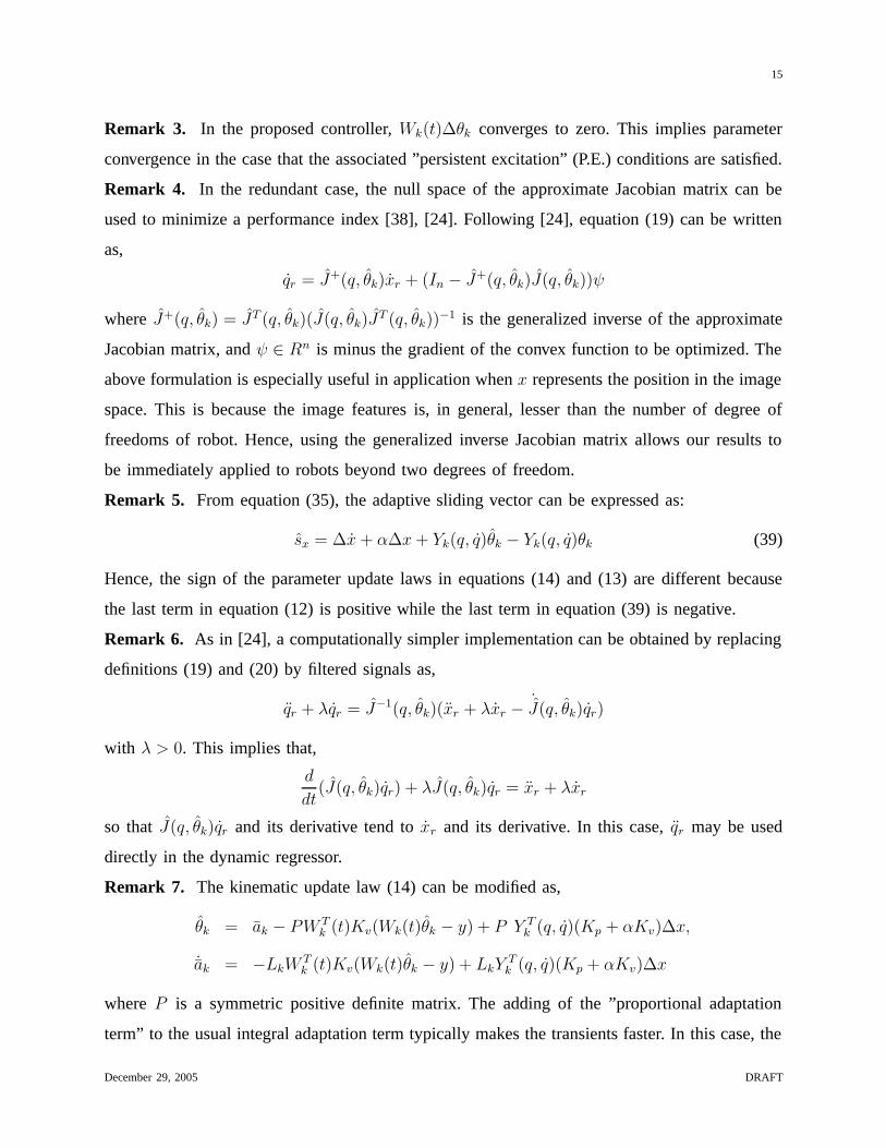
Next, we implemented the proposed controllers on a 2-link direct-drive robot as shown in

figure 3. The masses of the first and second links are approximately equal to 1.6kg and 1kg

respectively, and the masses of the first and second motors are approximately equal to 9.5kg and

3kg respectively. The lengths of the first and second links are approximately equal to l1 = 0.31m

and l2 = 0.3m respectively. The robot is holding an object with an length of 0.10m and a grasping

angle of 60o. A PSD camera (position sensitive detector) manufactured by Hamamatsu is used

to measure the position of the robot end effector.December 29, 2005 DRAFT

20

(X,Y)=(155, 75)

(X,Y)=(72, 188)

Fig. 2. Experimental results showing robot’s shadow following a line

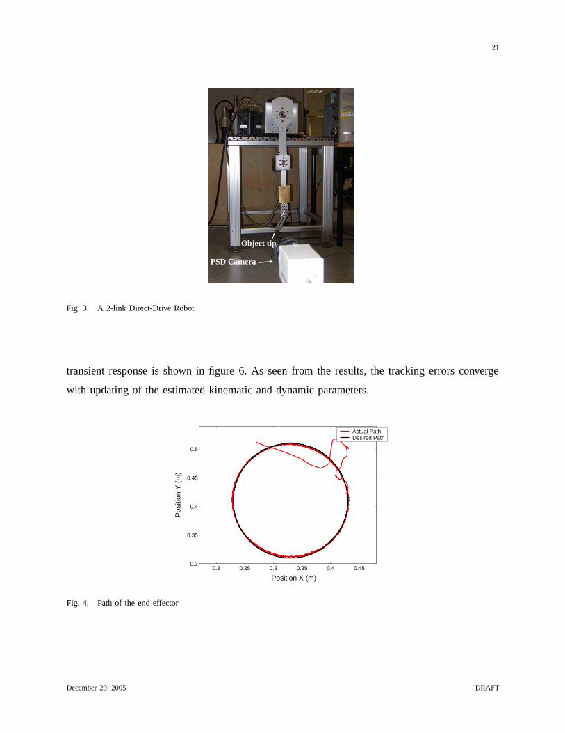
The robot is required to hold an object with uncertain length and grasping angle and follow

a circular trajectory specified in Cartesian space as:

Xd = 0.33 + 0.1 sin(0.54 + 3t)

Yd = 0.41 + 0.1 cos(0.54 + 3t)

In this experiment, uncertainties in both robot parameters and object parameters were also

considered. The link lengths were estimated as l1(0) = 0.25m, l2(0) = 0.27m and the object

length and grasping angle were estimated as 0.12 m and 20o respectively. The initial position of

the robot end effector was specified as (X(0), Y (0)) = (0.28, 0.52). Experimental results with

Lk = diag{0.04, 0.045, 0.015}, Ld = diag{0.01, 0.002, 0.002, 0.002, 0.015, 0.01, 0.01}, Kv =

diag{2, 2}, Kp = diag{450, 450}, α = 1.2, λ = 200π are presented in figures 4 and 5. The


21

Object tip

PSD Camera

Fig. 3. A 2-link Direct-Drive Robot

transient response is shown in figure 6. As seen from the results, the tracking errors converge

with updating of the estimated kinematic and dynamic parameters.

0.2 0.25 0.3 0.35 0.4 0.450.3

0.35

0.4

0.45

0.5

Position X (m)

Pos

ition

Y (

m)

Actual PathDesired Path

Fig. 4. Path of the end effector


22

0 2 4 6 8 10

−0.1

−0.05

0

0.05

0.1

0.15

Time (sec)

Pos

ition

err

or (

m)

X errorY error

Fig. 5. Position Errors

0 0.05 0.1 0.15 0.2 0.25 0.3

−0.1

−0.05

0

0.05

0.1

0.15

Time (sec)

Pos

ition

err

or (

m)

X errorY error

Fig. 6. Position Errors (Transient)

In the next experiments, a proportional term is added to the kinematic update law (see Remark

7). The experimental results in figure 7 and figure 8 show that the tracking errors converge and

the transient response is shown in figure 9. We used Lk = diag{0.075, 0.105, 0.025}, P =

diag{0.00018, 0.0002, 0.0001}, with the rest of the control gains remaining the same.


23

0.2 0.25 0.3 0.35 0.4 0.450.3

0.35

0.4

0.45

0.5

Position X (m)

Pos

ition

Y (

m)

Actual PathDesired Path

Fig. 7. Path of the end effector

0 2 4 6 8 10

−0.1

−0.05

0

0.05

0.1

0.15

Time (sec)

Tra

ckin

g E

rror

s (m

)

X errorY error

Fig. 8. Position Errors

0 0.05 0.1 0.15 0.2 0.25 0.3

−0.1

−0.05

0

0.05

0.1

0.15

Time (sec)

Tra

ckin

g E

rror

s (m

)

X errorY error

Fig. 9. Position Errors (Transient)


24

V. CONCLUDING REMARKS

We have proposed an adaptive Jacobian controller for robot tracking control with uncertain

kinematics and dynamics. A novel update law is introduced to update uncertain kinematics

parameters, using sensory feedback of the robot end effector position. The robot end effector is

able to track a desired trajectory with the uncertain kinematics and dynamics parameters being

updated online. Experimental results illustrate the performance of the proposed controllers. The

experiments also show that a robot can be controlled using its shadow. As pointed in [36],

the research on robot control with uncertain kinematics and dynamics is just at the beginning

stage [36]. Future works would be devoted to extending the adaptive Jacobian controller to

force tracking control and object manipulation by robot hand with soft tips. In these control

problems, the Jacobian matrices are uncertain. For example, the constraint Jacobian is uncertain

in presence of uncertainty in the constraint surface; the contact points of the robot fingers with

soft tips are also difficult to estimate exactly since they are changing during manipulation. Due

to the depressions at the soft contact points, the kinematics of the fingers also become uncertain.

It is also interesting to investigate the applicability of the proposed adaptive Jacobian control

theory to the study of internal model in sensorimotor integration [59], [60].

REFERENCES

[1] M.A. Arbib, N. Schweighofer, and W.T. Thach, ”Modeling the Cerebellum: From Adaptation to Coordination”, Motor

Control and Sensory-Motor Integration: Issues and Directions, (D.J. Glencross and J.P. Piek, Eds.), pp 11-36, Elsevier

Science, 1995.

[2] K. Sekiyama, S. Miyauchi, T. Imaruoka, H. Egusa, T. Tashiro, ”Body image as a visuomotor transformation device revealed

in adaptation to reversed vision”, Nature, vol. 407, pp 374-377, 2000.

[3] F. Pavani and U. Castiello, ”Binding personal and extrapersonal space through body shadows”, Nature Neuroscience, vol. 7,

pp. 14 - 16, 2004.

[4] A. Pouget, and L.H. Snyder, ”Computational approaches to sensorimotor transformations”, Nature Neuroscience, vol. 3,

pp 1192-1198, 2000.

[5] J. M. Hollerbach, “A recursive lagrangian formulation of manipulator dynamics and a comparative study of dynamics

formulation complexity,” IEEE Trans. on Systems, Man, and Cybernetics, vol. 10, 1980.

[6] J. Y. S. Luh, M. H. Walker, and R. P. Paul, “On-line computational scheme for mechanical manipulator,” Journal of

Dynamic Systems, Measurement, and Control, vol. 102, pp. 69–76, 1980.

[7] J. J. Craig, Introduction to Robotics. New York: Addison-Wesley, 1986.

[8] C.H. An, C. G. Atkeson, J.M. Hollerbach, ”Model-based control of a robot manipulator”, Cambridge, Mass.: MIT Press,

1988.


25

[9] J.M. Renders, E. Rossignol, M. Becquet, and R. Hanus, ”Kinematic calibration and geometrical parameter identification

for robots”, IEEE Transactions on Robotics and Automation, Vol. 7, No. 6, pp 721 - 732, 1991.

[10] M. Takegaki and S. Arimoto, “A new feedback method for dynamic control of manipulators,” ASME J. of Dynamic Systems,

Measurement and Control, vol. 102, pp. 119–125, 1981.

[11] S. Arimoto, Control Theory of Nonlinear Mechanical Systems - A Passivity-Based and Circuit-Theoretic Approach. Oxford:

Clarendon Press, 1996.

[12] J. J. Craig, P. Hsu, and S. S. Sastry, “Adaptive control of mechanical manipulators,” Int. J. Robotics Research, vol. 6,

no. 2, pp. 16–28, 1987.

[13] J. J. Craig, Adaptive Control of Mechanical Manipulators. New York: Addison-Wesley, 1988.

[14] J. J. E. Slotine and W. Li, “On the adaptive control of robot manipulators,” Int. J. Robotics Research, no. 6, pp. 49–59,

1987.

[15] J. J. E. Slotine and W. Li, “Adaptive manipulator control: A case study,” IEEE Trans. on Automatic Control, vol. 33,

no. 11, pp. 995–1003, 1988.

[16] J. J. E. Slotine and W. Li, ”Adaptive strategies in constrained manipulation”, in Proc. IEEE Int. Conf. on Robotics and

Automation, pp. 595 – 601, 1987.

[17] R. H. Middleton and G. C. Goodwin, “Adaptive computed torque control for rigid link manipulators,” Systems and Control

Letter, vol. 10, pp. 9–16, 1988.

[18] D. E. Koditschek, “Adaptive techniques for mechanical systems,” in Fifth Yale Workshop on Applications of Adaptive

Systems Theory, (New Haven, CT), pp. 259–265, 1987.

[19] J. T. Wen and D. Bayard, “New class of control laws for robotic manipulators -part 2. adaptive case,” International Journal

of Control, vol. 47, no. 5, pp. 1387–1406, 1988.

[20] B. Paden and R. Panja, “A globally asymptotically stable ’PD+’ controller for robot manipulator,” International Journal

of Control, vol. 47, no. 6, pp. 1697–1712, 1988.

[21] R. Kelly and R. Carelli, “Unified approach to adaptive control of robotic manipulators,” in Proc. 27th IEEE Conf. on

Decision and Control, 1988.

[22] R. Ortega and M. W. Spong, “Adaptive motion control of rigid robots: a tutorial,” Automatica, vol. 25, no. 6, pp. 877–888,

1989.

[23] N. Sadegh and R. Horowitz, “Stability and robustness analysis of a class of adaptive controllers for robotic manipulators,”

International Journal of Robotics Research, vol. 9, no. 3, pp. 74–92, 1990.

[24] G. Niemeyer and J.J.E. Slotine, ”Performance in Adaptive Manipulator Control,” Int. J. Robotics Research, vol. 10, no. 2,

1991.

[25] H. Berghuis, R. Ortega and H. Nijmeijer, ”A robust adaptive robot controller”, IEEE Transactions on Robotics and

Automation, vol. 9, no. 6, pp 825 - 830, 1993.

[26] L. L. Whitcomb, A. Rizzi, and D.E. Koditschek, ”Comparative Experiments with a New Adaptive Controller for Robot

Arms”, IEEE Transactions on Robotics and Automation, vol. 9, no. 1, pp 59-70, 1993.

[27] L. L. Whitcomb, S. Arimoto, T. Naniwa, and F. Ozaki, ”Experiments in Adaptive Model-Based Robot Force Control”,

IEEE Control Systems Magazine, vol. 16, no. 1, pp 49-57, 1996.

[28] K.W. Lee and H. Khalil, ”Adaptive output feedback control of robot manipulators using high gain observer”, Int. J. Control,

vol. 67, no. 6, 1997


26

[29] P. Tomei, “Robust adaptive friction compensation for tracking control of robot manipulators,” IEEE Transactions on

Automatic Control, vol. 45, no. 11, pp. 2164 – 2169, 2000.

[30] F. L. Lewis, C. T. Abdallah, and D. M. Dawson, Control of Robot Manipulators. New York: Macmillan Publishing

Company, 1993.

[31] L. Sciavicco and B. Siciliano, Modelling and control of robot manipulators. New York: Springer-Verlag, 2000.

[32] C. C. Cheah, S. Kawamura, and S. Arimoto, “Feedback control for robotic manipulators with an uncertain jacobian matrix,”

Journal of Robotic System, vol. 12, no. 2, pp. 119–134, 1999.

[33] H. Yazarel and C. C. Cheah, “Task-space adaptive control of robotic manipulators with uncertainties in gravity regressor

matrix and kinematics,” IEEE Trans. on Automatic Control, vol. 47, no. 9, pp. 1580 – 1585, 2002.

[34] C. C. Cheah, M. Hirano, S. Kawamura, and S. Arimoto, “Approximate jacobian control for robots with uncertain kinematics

and dynamics,” IEEE Trans. on Robotics and Automation, vol. 19, no. 4, pp. 692–702, 2003.

[35] W. E. Dixon, “Adaptive regulation of amplitude limited robot manipulators with uncertain kinematics and dynamics,” in

Proc. of American Control Conference, (Boston, USA), pp. 3939–3844, 2004.

[36] S. Arimoto, “Robotics research toward explication of everyday physics,” International Journal of Robotic Research, vol. 18,

no. 11, pp. 1056–1063, 1999.

[37] J. J. E. Slotine and W. Li, Applied nonlinear control. Englewood Cliffs, New Jersey: Prentice Hall, 1991.

[38] Y. Nakamura, Advanced Robotics. Reading MA: Addison-Wesleyn, 1985.

[39] G. H. S. Hutchinson and P. Corke, “A tutorial on visual servo control,” IEEE Trans. on Robotics and Automation, vol. 12,

no. 5, pp. 651 – 670, 1996.

[40] L. E. Weiss, A. C. Sanderson and C. P. Neuman, “Dynamic sensor-based control of robots with visual feedback,” IEEE

Trans. on Robotics and Automation, vol. RA-3, no. 5, pp. 404 – 417, 1987.

[41] B. Espiau, F. Chaumette and P. Rives, ”A new approach to visual servoing in robotics”, IEEE Trans. on Robotics and

Automation, Vol. 8 , No. 3, pp 313 - 326, 1992.

[42] N.P. Papanikolopoulos, P.K. Khosla, and T. Kanade, ”Visual tracking of a moving target by a camera mounted on a robot:

a combination of control and vision”, IEEE Trans. on Robotics and Automation, Vol. 9 , No. 1, pp 14 - 35, 1993.

[43] N.P. Papanikolopoulos and P.K. Khosla, ”Adaptive robotic visual tracking: theory and experiments”, IEEE Trans. on

Automatic Control, Vol. 38, No. 3, 429 - 445, 1993.

[44] M. Jgersand, O. Fuentes, R. Nelson, ”Acquiring Visual-Motor Models for Precision Manipulation with Robot Hands”, in

Proc of 4th European Conference on Computer Vision,pp 603-612, 1996.

[45] E. Malis, F. Chaumette and S. Boudet, ”2D 1/2 visual servoing”, IEEE Transaction on Robotics and Automation, Vol. 15,

No. 2, pp 234-246, April 1999.

[46] E. Malis and F. Chaumette, ”Theoretical improvements in the stability analysis of a new class of model-free visual servoing

methods”, IEEE Transaction on Robotics and Automation, Vol. 18, No. 2, pp 176-186, April 2002.

[47] K. Miura, K. Hashimoto, J. Gangloff, and M. de Mathelin, ”Visual servoing without Jacobian using modified simplex

optimization”, in Proc. of IEEE International Conference on Robotics and Automation, pp 3515-3529, (Barcelona, Spain),

2005.

[48] N.R. Gans, G. H. S. Hutchinson, P. Corke, ”Performance tests for visual servo control systems, with application to

partitioned approaches to visual servo control”, Int. J. Robotics Research, vol.10, no. 11,pp 955-981, 2003.

[49] B. Espiau, Effect of camera calibration errors on visual servoing in robotics, in Proc. of International Symposium on

Experimental Robotics, (Kyoto, Japan),r 1993.


27

[50] L. Deng, F. Janabi-Sharifi, and W. J. Wilson, Stability and robustness of visual servoing methods, in Proc. of IEEE

International Conference on Robotics and Automation, pp. 16051609, (Washington D.C.), 2002.

[51] E. Malis and P. Rives, ”Robustness of Image-Based Visual Servoing with Respect to Depth Distribution Errors”, in Proc.

of IEEE International Conference on Robotics and Automation, Taipei, Taiwan, September 2003.

[52] E. Malis, ”Visual servoing invariant to changes in camera intrinsic parameters”, IEEE Transaction on Robotics and

Automation, Vol. 20, No. 1, pp 72-81, 2004.

[53] W. Li, ”Adaptive control of robot manipulators”, Doctoral Thesis, MIT Dept. of Mechanical Engineering, June 1990.

[54] R. Sanner and J.J.E. Slotine, ”Gaussian Networks for Direct Adaptive Control,” IEEE. Trans. on Neural Networks, 3(6),

1992.

[55] F.L. Lewis, ”Neural network control of robot manipulators”, IEEE Expert: Intelligent Systems and Their Applications, vol.

11, no. 3, pp. 64-75, June 1996.

[56] C. C. Cheah, C. Liu and J.J.E. Slotine, ”Approximate Jacobian Adaptive Control for Robot Manipulators”, in Proc. of

IEEE Int. Conference on Robotics and Automation, (New Orleans, USA), pp 3075-3080, 2004.

[57] C. C. Cheah, C. Liu and J.J.E. Slotine, ”Experiments on Adaptive Control of Robots with Uncertain Kinematics and

Dynamics”, in Proc. of Int. Symposium on Experimental Robotics, (Singapore).

[58] P. Ioannou and J. Sun, ’Robust Adaptive Control’ Prentice Hall, 1996.

[59] C. Tin and C.S. Poon, ”Internal models in sensorimotor integration: Perspectives from adaptive control theory”, Journal

of Neural Engineering, Vol 2, no. 3, pp. S147-S163, 2005.

[60] H. Imamizu, Y. Uno and M. Kawato, ”Adaptive Internal Model of Intrinsic Kinematics Involved in Learning an Aiming

Task”, Journal of Experimental Psychology: Human Perception and Performance, Vol. 24, No. 3, pp. 812-829, 1998.


28

APPENDIX A: INDEX TO MULTIMEDIA EXTENSION

The multimedia extensions to this article are at: http://www.ijrr.org.

Extension Type Description

1 Video Experimental results of robot tracking control using shadow’s feedback.


adaptive tracking control for robots with unknown...

Documents