adaptive partial differential scott j. moura equation ...flyingv.ucsd.edu/papers/pdf/182.pdf ·...

Scott J. MouraUC President’s Postdoctoral Fellow

Mechanical and Aerospace Engineering,

University of California, San Diego,

San Diego, CA 92093

e-mail: [email protected]

Nalin A. ChaturvediSenior Research Engineer

Research and Technology Center,

Robert Bosch LLC,

Palo Alto, CA 94304


Miroslav KrsticProfessor

Mechanical and Aerospace Engineering,

University of California, San Diego,

San Diego, CA 92093


Adaptive Partial DifferentialEquation Observer for BatteryState-of-Charge/State-of-HealthEstimation Via anElectrochemical ModelThis paper develops an adaptive partial differential equation (PDE) observer for batterystate-of-charge (SOC) and state-of-health (SOH) estimation. Real-time state and parame-ter information enables operation near physical limits without compromising durability,thereby unlocking the full potential of battery energy storage. SOC/SOH estimation istechnically challenging because battery dynamics are governed by electrochemical prin-ciples, mathematically modeled by PDEs. We cast this problem as a simultaneous state(SOC) and parameter (SOH) estimation design for a linear PDE with a nonlinear outputmapping. Several new theoretical ideas are developed, integrated together, and tested.These include a backstepping PDE state estimator, a Pad�e-based parameter identifier,nonlinear parameter sensitivity analysis, and adaptive inversion of nonlinear outputfunctions. The key novelty of this design is a combined SOC/SOH battery estimation algo-rithm that identifies physical system variables, from measurements of voltage and currentonly. [DOI: 10.1115/1.4024801]

1 Introduction

This paper develops an adaptive PDE observer for combinedSOC and SOH estimation in batteries, using an electrochemicalmodel.

Accurate battery SOC estimation algorithms are currently ofextreme importance due to their applications in electrified trans-portation and energy storage systems for renewable sources. Therelevancy of this topic is further underscored by the 27.2 billionUSD federal government investment in energy efficiency andrenewable energy research, including advanced batteries, underthe American Recovery and Reinvestment Act of 2009. To guar-antee safety, durability, and performance, battery managementsystems within these advanced transportation and energy infra-structures must have accurate knowledge of internal batteryenergy levels [1]. Such knowledge enables them to efficientlyroute energy while satisfying power demands and device-leveloperating constraints [2].

Monitoring battery SOC and SOH is particularly challengingfor several technical reasons. First, directly measuring Li concen-tration or physical examination of cell components is impracticaloutside specialized laboratory environments [3,4]. Second, thedynamics are governed by partial differential algebraic equationsderived from electrochemical principles [5]. The only measurablequantities (voltage and current) are related to the states throughboundary values. Finally, the model’s parameters vary widelywith electrode chemistry, electrolyte, packaging, and time. In thispaper, we directly address these technical challenges. Namely, wedesign an adaptive observer using a reduced-form PDE modelbased upon electrochemical principles. As such, the algorithmestimates physical variables directly related to SOC and SOH, afirst to the authors’ knowledge.

Over the past decade research on battery SOC/SOH estimationhas experienced considerable growth. One may divide thisresearch by the battery models each algorithm employs.

The first category considers estimators based upon equivalentcircuit models (ECMs). These models use circuit elements tomimic the phenomenological behavior of batteries. For example,the work by Plett [6] applies an extended Kalman filter to simulta-neously identify the states and parameters of an ECM. Verbruggeand his co-workers used ECMs with combined coulomb-countingand voltage inversion techniques in Ref. [7] and adaptive parame-ter identification algorithms in Ref. [8]. More recently, a linearparameter varying approach was designed in Ref. [9]. The keyadvantage of ECMs is their simplicity. However, they oftenrequire extensive parameterization for accurate predictions. Thisoften produces models with nonphysical parameters, whose com-plexity becomes comparable to electrochemical models.

The second category considers electrochemical models, whichaccount for the diffusion, intercalation, and electrochemicalkinetics. Although these models can accurately predict internalstate variables, their mathematical structure is generally too com-plex for controller/observer design. Therefore, these approachescombine model reduction and estimation techniques. Some of thefirst studies within this category use a “single particle model”(SPM) of electrochemical battery dynamics in combination withan extended Kalman filter [10,11]. Another approach is to employresidue grouping for model reduction and linear Kalman filters forobservers [12]. The authors of Ref. [13] apply simplifications tothe electrolyte and solid phase concentration dynamics to performSOC estimation. To date, however, simultaneous SOC and SOHestimation using electrochemical models remains an openquestion.

In this paper, we extend the aforementioned research bydesigning an electrochemical model based adaptive observer forsimultaneous SOC/SOH estimation. Several novel theoreticalideas are developed, integrated, and tested. These include aPDE backstepping state estimator, Pad�e-based PDE parameter

Contributed by the Dynamic Systems Division of ASME for publication in theJOURNAL OF DYNAMIC SYSTEMS, MEASUREMENT, AND CONTROL. Manuscript receivedJuly 18, 2012; final manuscript received June 8, 2013; published online October 15,2013. Assoc. Editor: Yang Shi.

Journal of Dynamic Systems, Measurement, and Control JANUARY 2014, Vol. 136 / 011015-1Copyright VC 2014 by ASME

Downloaded From: http://dynamicsystems.asmedigitalcollection.asme.org/ on 11/16/2013 Terms of Use: http://asme.org/terms

identifier, nonlinear identifiability analysis of the output equation,and adaptive output function inversion. This paper extends ourprevious work [14–16] by including estimator validation resultsagainst a high-fidelity battery simulator. The final result is anadaptive observer for simultaneous SOC/SOH estimation whichidentifies physical battery system variables, from current and volt-age measurements only.

The paper is organized as follows: Sec. 2 describes the singleparticle model. Sections 3–6 describe the subsystems of theadaptive observer, including the state estimator, PDE parameteridentifier, output function parameter identifier, and adaptive out-put function inversion. Section 7 presents simulation results todemonstrate the observer’s performance. Section 8 providesguidelines for selecting gains. Finally, Sec. 9 summarizes the keycontributions.

2 Electrochemical Cell Model and Analysis

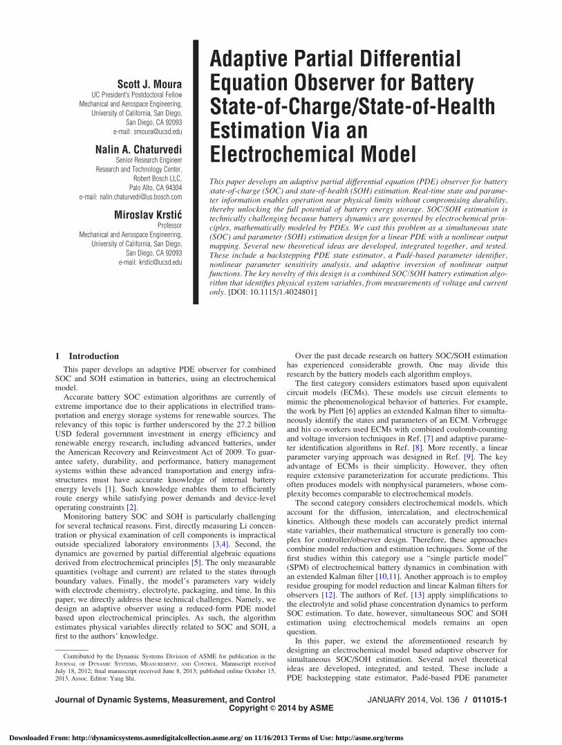
The SPM was first applied to lithium battery systems inRef. [17] and is the model we utilize in this paper. The key idea isthat the solid phase of each electrode can be idealized as a singlespherical particle. This model results if one assumes the electro-lyte Li concentration is constant in space and time [1]. Thisassumption works well for small currents or electrolytes withlarge electronic conductivities. However, it induces errors at largeC-rates [1]. Moreover, we assume constant temperature. Figure 1provides a schematic of the SPM concept. Mathematically, themodel consists of two diffusion PDEs governing each electrode’sconcentration dynamics, where input current enters as a Neumannboundary condition. Output voltage is given by a nonlinear func-tion of the state values at the boundary and the input current.

Although this model captures less dynamic behavior than otherelectrochemical-based estimation models [17], its mathematicalstructure is amenable to adaptive observer design.

2.1 Single Particle Model. Diffusion in each electrode isgoverned by Fick’s law in spherical coordinates

@c�s@tðr; tÞ ¼ D�s

2

r

@c�s@rðr; tÞ þ @

2c�s@r2ðr; tÞ

� �(1)

@cþs@tðr; tÞ ¼ Dþs

2

r

@cþs@rðr; tÞ þ @

2cþs@r2ðr; tÞ

� �(2)

with Neumann boundary conditions

@c�s@rð0; tÞ ¼ 0;

@c�s@rðR�s ; tÞ ¼

IðtÞD�s Fa�AL�

(3)

@cþs@rð0; tÞ ¼ 0;

@cþs@rðRþs ; tÞ ¼ �

IðtÞDþs FaþALþ

(4)

The Neumann boundary conditions at r ¼ Rþs and r ¼ R�s signifythat the flux entering the electrode is proportional to the input cur-rent I(t). The Neumann boundary conditions at r¼ 0 are requiredfor well-posedness. Note that the states for the two PDEs aredynamically uncoupled, although they have proportional bound-ary inputs.

The measured terminal voltage output is governed by a combi-nation of electric overpotential, electrode thermodynamics, andButler-Volmer kinetics. The end result is

VðtÞ ¼ RT

aFsinh�1 IðtÞ

2aþALþiþ0 ðcþssðtÞÞ

� �� RT

aFsinh�1 IðtÞ

2a�AL�i�0 ðc�ssðtÞÞ

� �þ UþðcþssðtÞÞ � U�ðc�ssðtÞÞ þ Rf IðtÞ (5)

where the exchange current density ij0 and solid-electrolyte sur-face concentration cj

ss are, respectively

ij0ðcj

ssÞ ¼ kjffiffiffiffiffiffiffiffiffiffiffiffiffiffiffiffiffiffiffiffiffiffiffiffiffiffiffiffiffiffiffiffiffiffiffiffiffiffiffiffiffiffiffiffiffic0

ecjssðtÞðcj

s;max � cjssðtÞÞ

q(6)

cjssðtÞ ¼ cj

sðRjs; tÞ; j 2 fþ;�g (7)

The functions Uþð�Þ and U�ð�Þ in Eq. (5) are the equilibriumpotentials of each electrode material, given the surface concentra-tion. Mathematically, these are strictly monotonically decreasingfunctions of their input. This fact implies that the inverse of itsderivative is always finite, a property which we require in Sec. 6.Further details on the electrochemical principles used to derivethese equations can be found in Refs. [1,5].

This model contains the property that the total number of lith-ium ions is conserved [13]. Mathematically, ðd=dtÞðnLiÞ ¼ 0,where

nLi ¼eþs LþA

4

3pðRþs Þ

3

ðRþs

0

4pr2cþs ðr; tÞdr þ e�s L�A4

3pðR�s Þ

3

ðR�s

0

4pr2c�s ðr; tÞdr

(8)

This property will become important, as it relates the total concen-tration of lithium in the cathode and anode. We leverage this factto perform model reduction in the state estimation problem.

2.2 Model Comparison. The SPM approximation increasesin accuracy as C-rate decreases and/or as electrolyte conductivityincreases. Here, we demonstrate how the SPM’s accuracydegrades as C-rate increases, compared to a full order electro-chemical model.

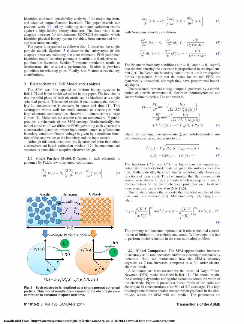
A simulator has been created for the so-called Doyle-Fuller-Newman (DFN) model described in Ref. [1]. This model retainsthe electrolyte dynamics and spatial dynamics across the width ofthe electrode. Figure 2 presents a freeze-frame of the solid andelectrolyte Li concentrations after 50 s of 5 C discharge. This highdischarge rate induces notable concentration gradients in the elec-trolyte, which the SPM will not predict. The parameters are

Fig. 1 Each electrode is idealized as a single porous sphericalparticle. This model results from assuming the electrolyte con-centration is constant in space and time.

011015-2 / Vol. 136, JANUARY 2014 Transactions of the ASME


identical to those used in the publicly available DUALFOILmodel, developed by Newman and his collaborators [18]. ThisDFN model also serves as the generator of experimental data toevaluate the adaptive observer’s performance.

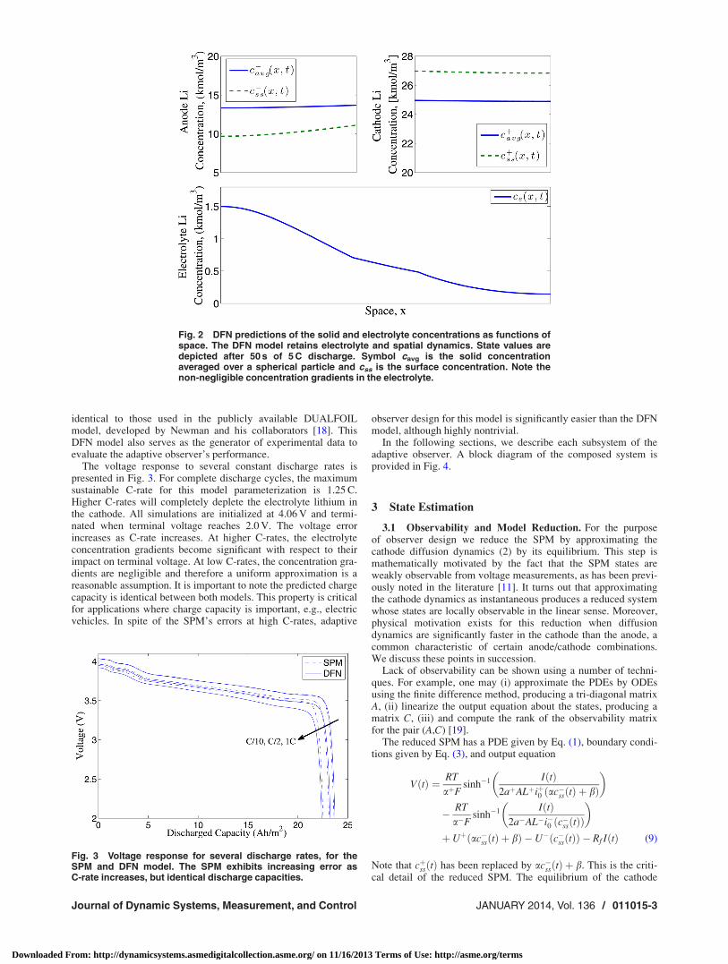
The voltage response to several constant discharge rates ispresented in Fig. 3. For complete discharge cycles, the maximumsustainable C-rate for this model parameterization is 1.25 C.Higher C-rates will completely deplete the electrolyte lithium inthe cathode. All simulations are initialized at 4.06 V and termi-nated when terminal voltage reaches 2.0 V. The voltage errorincreases as C-rate increases. At higher C-rates, the electrolyteconcentration gradients become significant with respect to theirimpact on terminal voltage. At low C-rates, the concentration gra-dients are negligible and therefore a uniform approximation is areasonable assumption. It is important to note the predicted chargecapacity is identical between both models. This property is criticalfor applications where charge capacity is important, e.g., electricvehicles. In spite of the SPM’s errors at high C-rates, adaptive

observer design for this model is significantly easier than the DFNmodel, although highly nontrivial.

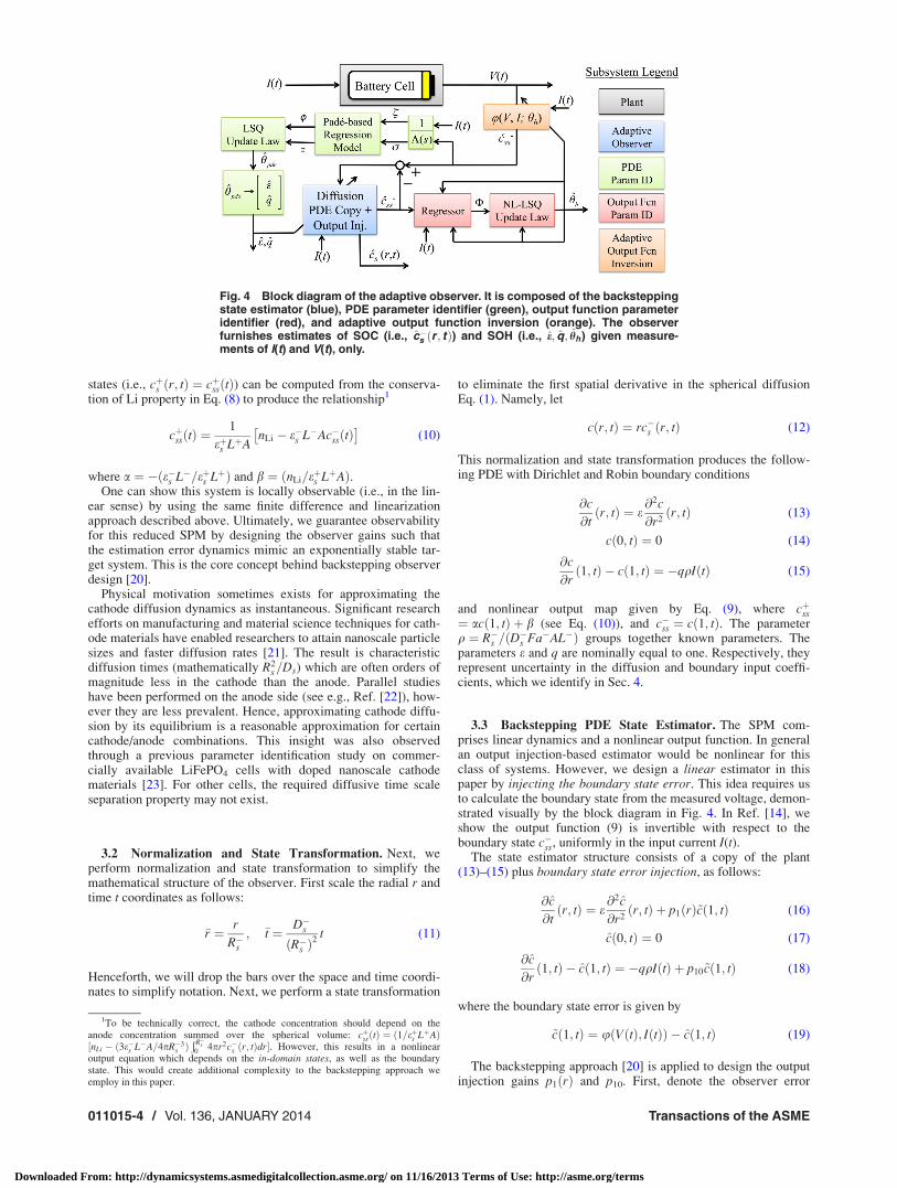
In the following sections, we describe each subsystem of theadaptive observer. A block diagram of the composed system isprovided in Fig. 4.

3 State Estimation

3.1 Observability and Model Reduction. For the purposeof observer design we reduce the SPM by approximating thecathode diffusion dynamics (2) by its equilibrium. This step ismathematically motivated by the fact that the SPM states areweakly observable from voltage measurements, as has been previ-ously noted in the literature [11]. It turns out that approximatingthe cathode dynamics as instantaneous produces a reduced systemwhose states are locally observable in the linear sense. Moreover,physical motivation exists for this reduction when diffusiondynamics are significantly faster in the cathode than the anode, acommon characteristic of certain anode/cathode combinations.We discuss these points in succession.

Lack of observability can be shown using a number of techni-ques. For example, one may (i) approximate the PDEs by ODEsusing the finite difference method, producing a tri-diagonal matrixA, (ii) linearize the output equation about the states, producing amatrix C, (iii) and compute the rank of the observability matrixfor the pair (A,C) [19].

The reduced SPM has a PDE given by Eq. (1), boundary condi-tions given by Eq. (3), and output equation

VðtÞ ¼ RT

aþFsinh�1 IðtÞ

2aþALþiþ0 ðac�ssðtÞ þ bÞ

� �� RT

a�Fsinh�1 IðtÞ


� �þ Uþðac�ssðtÞ þ bÞ � U�ðc�ssðtÞÞ � Rf IðtÞ (9)

Note that cþssðtÞ has been replaced by ac�ssðtÞ þ b. This is the criti-cal detail of the reduced SPM. The equilibrium of the cathode

Fig. 2 DFN predictions of the solid and electrolyte concentrations as functions ofspace. The DFN model retains electrolyte and spatial dynamics. State values aredepicted after 50 s of 5 C discharge. Symbol cavg is the solid concentrationaveraged over a spherical particle and css is the surface concentration. Note thenon-negligible concentration gradients in the electrolyte.

Fig. 3 Voltage response for several discharge rates, for theSPM and DFN model. The SPM exhibits increasing error asC-rate increases, but identical discharge capacities.

Journal of Dynamic Systems, Measurement, and Control JANUARY 2014, Vol. 136 / 011015-3


states (i.e., cþs ðr; tÞ ¼ cþssðtÞ) can be computed from the conserva-tion of Li property in Eq. (8) to produce the relationship1

cþssðtÞ ¼1

eþs LþAnLi � e�s L�Ac�ssðtÞ� �

(10)

where a ¼ �ðe�s L�=eþs LþÞ and b ¼ ðnLi=eþs LþAÞ.One can show this system is locally observable (i.e., in the lin-

ear sense) by using the same finite difference and linearizationapproach described above. Ultimately, we guarantee observabilityfor this reduced SPM by designing the observer gains such thatthe estimation error dynamics mimic an exponentially stable tar-get system. This is the core concept behind backstepping observerdesign [20].

Physical motivation sometimes exists for approximating thecathode diffusion dynamics as instantaneous. Significant researchefforts on manufacturing and material science techniques for cath-ode materials have enabled researchers to attain nanoscale particlesizes and faster diffusion rates [21]. The result is characteristicdiffusion times (mathematically R2

s=Ds) which are often orders ofmagnitude less in the cathode than the anode. Parallel studieshave been performed on the anode side (see e.g., Ref. [22]), how-ever they are less prevalent. Hence, approximating cathode diffu-sion by its equilibrium is a reasonable approximation for certaincathode/anode combinations. This insight was also observedthrough a previous parameter identification study on commer-cially available LiFePO4 cells with doped nanoscale cathodematerials [23]. For other cells, the required diffusive time scaleseparation property may not exist.

3.2 Normalization and State Transformation. Next, weperform normalization and state transformation to simplify themathematical structure of the observer. First scale the radial r andtime t coordinates as follows:

�r ¼ r

R�s; �t ¼ D�s

ðR�s Þ2

t (11)

Henceforth, we will drop the bars over the space and time coordi-nates to simplify notation. Next, we perform a state transformation

to eliminate the first spatial derivative in the spherical diffusionEq. (1). Namely, let

cðr; tÞ ¼ rc�s ðr; tÞ (12)

This normalization and state transformation produces the follow-ing PDE with Dirichlet and Robin boundary conditions

@c

@tðr; tÞ ¼ e

@2c

@r2ðr; tÞ (13)

cð0; tÞ ¼ 0 (14)

@c

@rð1; tÞ � cð1; tÞ ¼ �qqIðtÞ (15)

and nonlinear output map given by Eq. (9), where cþss¼ acð1; tÞ þ b (see Eq. (10)), and c�ss ¼ cð1; tÞ. The parameterq ¼ R�s =ðD�s Fa�AL�Þ groups together known parameters. Theparameters e and q are nominally equal to one. Respectively, theyrepresent uncertainty in the diffusion and boundary input coeffi-cients, which we identify in Sec. 4.

3.3 Backstepping PDE State Estimator. The SPM com-prises linear dynamics and a nonlinear output function. In generalan output injection-based estimator would be nonlinear for thisclass of systems. However, we design a linear estimator in thispaper by injecting the boundary state error. This idea requires usto calculate the boundary state from the measured voltage, demon-strated visually by the block diagram in Fig. 4. In Ref. [14], weshow the output function (9) is invertible with respect to theboundary state c�ss, uniformly in the input current I(t).

The state estimator structure consists of a copy of the plant(13)–(15) plus boundary state error injection, as follows:

@c

@tðr; tÞ ¼ e

@2c

@r2ðr; tÞ þ p1ðrÞ~cð1; tÞ (16)

cð0; tÞ ¼ 0 (17)

@c

@rð1; tÞ � cð1; tÞ ¼ �qqIðtÞ þ p10~cð1; tÞ (18)

where the boundary state error is given by

~cð1; tÞ ¼ uðVðtÞ; IðtÞÞ � cð1; tÞ (19)

The backstepping approach [20] is applied to design the outputinjection gains p1ðrÞ and p10. First, denote the observer error

Fig. 4 Block diagram of the adaptive observer. It is composed of the backsteppingstate estimator (blue), PDE parameter identifier (green), output function parameteridentifier (red), and adaptive output function inversion (orange). The observerfurnishes estimates of SOC (i.e., c�s ðr ; tÞ) and SOH (i.e., e; q; hh) given measure-ments of I(t) and V(t), only.

1To be technically correct, the cathode concentration should depend on theanode concentration summed over the spherical volume: cþssðtÞ ¼ ð1=eþs LþAÞ½nLi � ð3e�s L�A=4pR�3

s ÞÐ R�s

04pr2c�s ðr; tÞdr�. However, this results in a nonlinear

output equation which depends on the in-domain states, as well as the boundarystate. This would create additional complexity to the backstepping approach weemploy in this paper.



as ~cðr; tÞ ¼ cðr; tÞ � cðr; tÞ. Subtracting Eqs. (16)–(18) fromEqs. (13) to (15) produces the estimation error dynamics

@~c

@tðr; tÞ ¼ e

@2~c

@r2ðr; tÞ � p1ðrÞ~cð1; tÞ (20)

~cð0; tÞ ¼ 0 (21)

@~c

@rð1; tÞ � ~cð1; tÞ ¼ �p10~cð1; tÞ (22)

The backstepping approach seeks to find the upper-triangulartransformation

~cðr; tÞ ¼ ~wðr; tÞ �ð1

r

pðr; sÞ~wðsÞds (23)

which satisfies the exponentially stable target system

@ ~w

@tðr; tÞ ¼ e

@2 ~w

@r2ðr; tÞ þ k~wðr; tÞ (24)

~wð0; tÞ ¼ 0 (25)

@ ~w

@rð1; tÞ ¼ � 1

2~wð1; tÞ (26)

where k < e=4. The symbol k is a design parameter that enablesus to adjust the pole placement of the observer. The coefficient�1/2 in Eq. (26) ensures the target system is exponentially stable,as can be seen by the derivation below.

One can show that Eqs. (24)–(26) is exponentially stable in thespatial L2 norm by considering the Lyapunov function

WðtÞ ¼ 1

2

ð1

0

~w2ðr; tÞdr (27)

Taking the total time derivative and applying integration by partsyields

_WðtÞ ¼ � e2

~w2ð1Þ � eð1

0

~w2r dr þ k

ð1

0

~w2dr (28)

Recalling the Poincar�e inequality

� eð1

0

~w2r dr � e

2~w2ð1Þ � e

4

ð1

0

~w2dr (29)

produces

_WðtÞ � � e4� k

ð1

0

~w2dr ¼ � e2� 2k

WðtÞ (30)

which by the comparison principle [24] implies WðtÞ � Wð0Þexp½�ðe=2� 2kÞt� or ~wðtÞk k � ~wð0Þk k exp½�ðe=4� kÞt�. Hence,the target system is exponentially stable for k < e=4.

Remark 1. Using separation of variables, one may show theeigenvalues for the target system, (and hence the error system) arek� ey2, where y is given by the solutions of yþ 1

2tanðyÞ ¼ 0.

Consequently, the eigenvalues have zero imaginary parts. Ask! �1, the eigenvalue spectrum translates toward �1.

Following the procedure outlined in Ref. [20], we find that thekernel p(r, s) in Eq. (23) must satisfy the following conditions:

prrðr; sÞ � pssðr; sÞ ¼ke

pðr; sÞ (31)

pð0; sÞ ¼ 0 (32)

pðr; rÞ ¼ k2e

r (33)

defined on the domain D ¼ fðr; sÞj0 � r � s � 1g. The outputinjection gains are

p1ðrÞ ¼ �psðr; 1Þ �1

2pðr; 1Þ (34)

p10 ¼3� k=e

2(35)

These conditions compose a Klein-Gordon PDE, which coinci-dentally has an analytic solution given by

pðr; sÞ ¼ ke

rI1ð

ffiffiffiffiffiffiffiffiffiffiffiffiffiffiffiffiffiffiffiffiffiffiffiffik=eðr2 � s2Þ

pÞffiffiffiffiffiffiffiffiffiffiffiffiffiffiffiffiffiffiffiffiffiffiffiffi

k=eðr2 � s2Þp (36)

Solution Eq. (36) can be derived by converting the PDE into anequivalent integral equation and applying the method of succes-sive approximations [20]. Ultimately, this closed form solutionprovides the following output injection gains:

p1ðrÞ ¼�kr

2ezI1ðzÞ �

2kez

I2ðzÞ� �

(37)

where z ¼ffiffiffiffiffiffiffiffiffiffiffiffiffiffiffiffiffiffiffiffikeðr2 � 1Þ

r(38)

p10 ¼1

23� k

e

� �(39)

and I1ðzÞ and I2ðzÞ are, respectively, the first and second ordermodified Bessel functions of the first kind.

To complete the design, we need to establish that stability ofthe target system Eqs. (24)–(26) implies stability of the error sys-tem (20)–(22). That is, we must show the transformation (23) isinvertible. Toward this end, write the inverse transformation as

~wðr; tÞ ¼ ~cðr; tÞ þð1

r

lðr; sÞ~cðsÞds (40)

Following the same approach used to derive the direct transforma-tion kernel (36), we find that the inverse transformation kernel hasthe analytic solution

lðr; sÞ ¼ ke

rJ1ð

ffiffiffiffiffiffiffiffiffiffiffiffiffiffiffiffiffiffiffiffiffiffiffiffik=eðr2 � s2Þ

pÞffiffiffiffiffiffiffiffiffiffiffiffiffiffiffiffiffiffiffiffiffiffiffiffi

k=eðr2 � s2Þp (41)

where J1 is the first order Bessel function of the first kind. Wenow state the main result for the backstepping state estimator.

THEOREM 1. Consider the plant model (13)–(15) with observer(16)–(19) and estimation gains (37)–(39). Then 9k < e=4 suchthat the origin of the error system ~c ¼ 0 is exponentially stable inthe L2ð0; 1Þ norm.

Remark 2. Note that the estimator is linear in the state becausewe use the boundary state for error injection. The plant boundarystate is computed by inverting the nonlinear output mapping withrespect to the boundary state, given a current input (i.e.,uðVðtÞ; IðtÞÞ). The output function inversion is discussed in detailin Sec. 6.

Remark 3. Note the parameters e in Eqs. (16), (37)–(39) and qin Eq. (18). In the subsequent section, we design an identifier forthese parameters. We form an adaptive observer by replacingthese parameters with their estimates, via the certainty equiva-lence principle [25].

4 PDE Parameter Identification

Next, we design an identification algorithm for the diffusionand boundary input coefficients in Eqs. (13) and (15), respec-tively. Identification of the diffusion coefficient e from boundary



measurements is a significant fundamental challenge [26], for thefollowing reason. In finite-dimensional state-space systems, wetypically write the system in observable canonical form. Thisstructure enables one to uniquely identify state-space parametersfrom input–output data. In our problem, we require a parametricmodel where the diffusion coefficient multiplies measured dataonly. Otherwise, we have a nonlinear problem, since unknownstates are multiplied by unknown parameters. There is no clearway to do this for PDEs. This motivates our new contribution: uti-lizing a reduced-order model (Pad�e approximation) for the param-eter identification.

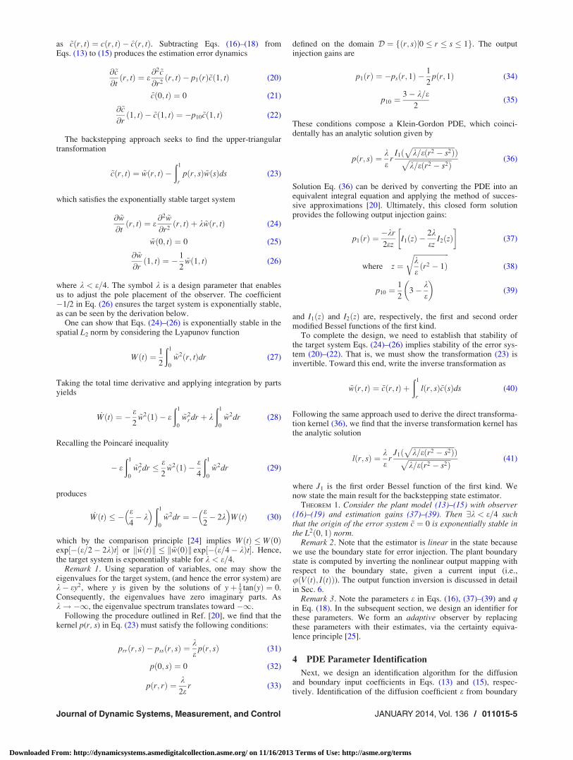
4.1 Pad�e Approximates. The PDE model Eqs. (13)–(15) canbe written in the frequency domain as a transcendental transferfunction

GðsÞ ¼ cssðsÞIðsÞ ¼

�qq sinhffiffiffiffiffiffiffis=e

p ffiffiffiffiffiffiffis=e

p cosh

ffiffiffiffiffiffiffis=e

p � sinh

ffiffiffiffiffiffiffis=e

p (42)

We now apply Pad�e approximations of the transcendental trans-fer function (42). Pad�e approximants represent a function by aratio of two power series. The defining characteristic of a Pad�e ap-proximate is that its Taylor series matches the Taylor series of thefunction it is approximating. Another useful property of Pad�eapproximates is that they naturally contain poles and zeros. ThePad�e expansion takes the following form:

GðsÞ ¼ limN!1

XN

k¼0

bksk

1þXN

k¼1

aksk

(43)

Figure 5 provides bode plots of G(s) and several Pad�e approxi-mates. Their analytical expressions are supplied in Table 1. ThePad�e approximates capture low frequency dynamics well. Accu-racy at high frequency increases as the Pad�e order increases. Welow-pass filter the input–output signals such that data are retainedwhere the Pad�e approximation is sufficiently accurate.

Our immediate goal is to design a parameter identificationscheme for the Pad�e approximation of the original PDE model.

4.2 Least Squares Identification. We utilize the first orderPad�e approximant as the nominal model. Namely

CssðsÞIðsÞ � P1ðsÞ ¼

�3qqe� 27

qqs

sþ 1

35es2

(44)

Assuming zero initial conditions and applying the inverse Laplacetransform produces the following linearly parameterized model:

1

35€cssðtÞ ¼ �e _cssðtÞ � 3qqe2IðtÞ � 2

7qqe _IðtÞ (45)

Since the parametric model contains time derivatives of measuredsignals, we employ filters [25] to avoid differentiation as follows:

_r1 ¼ r2 (46)

_r2 ¼ �k0r1 � k1r2 þ css (47)

_f1 ¼ f2 (48)

_f2 ¼ �k0f1 � k1f2 þ I (49)

where the polynomial KðsÞ ¼ s2 þ k1sþ k0 is chosen Hurwitz.One can analytically show that selecting the roots of KðsÞ resultsin a trade-off between convergence rate (via level of persistenceof excitation) and parameter bias (error induced by Pad�e approxi-mation). Consequently, the parametric model is given by

1

35�k0r1 � k1r2 þ cssð Þ ¼ �3qqe2f1 �

2

7qqef2 � er2 (50)

Let us denote the vector of unknown parameters by

hpde ¼ qe2 qe e� �T

(51)

Then, the parametric model can be expressed in matrix form aszpde ¼ hT

pde/, where

zpde ¼1

35�k0r1 � k1r2 þ cssð Þ (52)

/ ¼ �3qf1 � 2

7qf2 � r2

� �T

(53)

Given this linearly parameterized model, we choose a least-squares update law of the form [25]

_hpde ¼ Ppde

zpde � hTpde/

m2pde

/ (54)

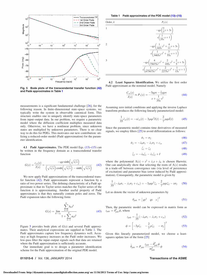
Table 1 Pad�e approximates of the PDE model (13)–(15)

Order, k PkðsÞ

1 �qq2

7sþ 3e

� �s

1

35esþ 1

� �2 �qq

1

165es2 þ 4

11sþ 3e

� �s

1

3465e2s2 þ 3

55esþ 1

� �3 �qq

4

75075e2s3 þ 2

195es2 þ 2

5sþ 3e

� �s

1

675675e3s3 þ 2

2275e2s2 þ 1

15esþ 1

� �

Fig. 5 Bode plots of the transcendental transfer function (42)and Pad�e approximates in Table 1



_Ppde ¼ �Ppde//T

m2pde

Ppde; Ppdeð0Þ ¼ Ppde0 ¼ PTpde0 > 0 (55)

m2pde ¼ 1þ cpde/

T/; cpde > 0 (56)

4.2.1 Managing Overparameterization With the Moore-Penrose Pseudoinverse. An important implementation issue withthe proposed Pad�e approximation approach is overparameteriza-tion. That is, the physical parameters must be uniquely determinedfrom the parameter vector hpde

hpde ¼cqe2bqee

24 35! eq

� �¼ heq (57)

Coincidently, the particular nonlinear form (products and powers)of the elements in vector hpde allows us to write a set of linearequations using a logarithmic nonlinear transformation and prop-erties of the logarithm function

2 1

1 1

1 0

24 35 log elog q

� �¼

log cqe2

log bqeð Þlog eð Þ

264375 (58)

which we re-write into compact notation as

AeqlogðheqÞ ¼ logðhpdeÞ (59)

where logðhÞ ¼ ½logðh1Þ; logðh2Þ; :::�T is an element-wise opera-tor. The parameter vector heq can be uniquely solved fromEq. (58) via the Moore-Penrose pseudoinverse. Thus

logðheqÞ ¼ ðATeqAeqÞ�1AT

eqlogðhpdeÞ (60)

This method works well in practice with respect to feeding param-eter estimates into the adaptive observer (lower-left-hand block inFig. 4), since the pseudoinverse ultimately involves computation-ally efficient matrix algebra.

5 Output Function Parameter Identification

The greatest difficulty in battery estimation arguably stemsfrom the nonlinear relationship between SOC and voltage [9]. Wedirectly address this difficulty by developing an identificationalgorithm for the uncertain parameters in the nonlinearly parame-terized output function (9). First, we analyze parameter identifi-ability to assess which subset of parameters is uniquelyidentifiable. Second, we apply nonlinear least squares to thissubset.

5.1 Identifiability. A necessary first step in nonlinear param-eter identification is a parameter sensitivity analysis. We specifi-cally apply the ranking procedure outlined in Ref. [27] to assesslinear dependence. Consider the output function (9) written inparametric form:

hðt; hÞ ¼ VðtÞ ¼ RT

aFsinh�1 h2IðtÞ

2ffiffiffiffiffiffiffiffiffiffiffiffiffiffiffiffiffiffiffiffiffiffiffiffiffiffiffiffiffiffiffiffiffiffiffiffiffiffiffiffiffiffiffiffiffiffiffiffiffiffiffiffifficþssðt; h1Þðcþs;max � cþssðt; h1ÞÞ

q264

375� RT

aFsinh�1 h3IðtÞ

2ffiffiffiffiffiffiffiffiffiffiffiffiffiffiffiffiffiffiffiffiffiffiffiffiffiffiffiffiffiffiffiffiffiffiffiffiffiffiffiffiffic�ssðtÞðc�s;max � c�ssðtÞÞ

q264

375þ Uþðcþssðt; h1ÞÞ � U�ðc�ssðtÞÞ þ h4IðtÞ

(61)

where cþssðt; h1Þ and the parameter vector h are

cþssðt; h1Þ ¼ �e�s L�

eþs Lþc�ssðtÞ þ

h1

eþs LþA;

h ¼ nLi;1

aþALþkþffiffiffiffiffic0

e

p ;1

a�AL�k�ffiffiffiffiffic0

e

p ;Rf

" #T

(62)

We have selected the elements of h because diminishing nLi

physically models capacity fade and increasing values for theother parameters capture various forms of internal resistance.

The following sensitivity analysis is performed in discrete time,since the required data is supplied in discrete time. Let kindex time such that t ¼ kDT; k 2 1; 2; :::; nT . The sensitivity ofthe output with respect to variations in the parameter hi at timeindex k is defined as Si;k ¼ @hðkDT; hÞ=@hi. For each parameterhi, stack the sensitivities at time indices k ¼ 1; 2;…; nT , i.e.,

Si ¼ ½Si;1; Si;2;…; Si;nT�T . Denote S ¼ ½S1; S2; S3; S4�, such that

S 2 RnT�4. A particular decomposition of STS reveals usefulinformation about linear dependence between parameters. Let

STS ¼ DTCD where

D ¼

S1k k 0 0 0

0 S2k k 0 0

0 0 S3k k 0

0 0 0 S4k k

2666437775;

C ¼

1hS1; S2iS1k k S2k k

hS1; S3iS1k k S3k k

hS1; S4iS1k k S4k k

hS2; S1iS2k k S1k k


hS2; S4iS2k k S4k k

hS3; S1iS3k k S1k k

hS3; S2iS3k k S2k k


hS4; S1iS4k k S1k k

hS4; S2iS4k k S2k k

hS4; S3iS4k k S3k k

1

26666666666664

37777777777775

(63)

where �k k denotes the Euclidian norm and h�; �i is the inner prod-uct. By the Cauchy Schwarz inequality �1 � ðhSi; Sji=

Sik k Sj

�� Þ � 1. This has the interpretation that values ofðhSi; Sji= Sik k Sj

�� Þ near �1 or 1 imply strong linear dependencebetween parameters hi and hj, whereas values near zero implyorthogonality.

An example for the matrix C is provided in Eq. (64). Thisexample analyzes parameter sensitivity for a UDDS drive cycledata set applied to the SPM battery model.

C ¼

1 �0:3000 0:2908 0:2956

�0:3000 1 �0:9801 �0:9805

0:2908 �0:9801 1 0:9322

0:2956 �0:9805 0:9322 1

26643775 (64)

Note that strong linear dependence exists between h2; h3; h4. Thisproperty is uniformly true across various drive cycles (e.g., US06,SC04, LA92, and naturalistic microtrips). This means it is difficultto determine how each individual parameter value changes,amongst these three parameters. As a result, we identify only twoparameters, nLi and Rf.

Remark 4. Coincidently, the parameters nLi and Rf representcapacity and power fade, respectively. Identification of nLi and Rf

provides a direct system-level measurement of SOH—a particu-larly beneficial feature of this design.

Remark 5. Indeed, the matrix STS has an important interpreta-tion in statistical mathematics—the inverse of the Fisher informa-tion matrix. From this interpretation, one may use the Cramer Raolower bound to compute the individual variance contribution ofeach parameter [27].



5.2 Nonlinear Least Squares. Now our immediate goal is toidentify the parameter vector hh ¼ nLi Rf

� �Tvia a nonlinear

least squares identification algorithm. Define ~hh ¼ hh � hh andwrite Eq. (61) in terms of ~hh

Vðt; hhÞ ¼RT

aFsinh�1 IðtÞ

2aþALþiþ0 ðcþssðt; ~hh1 þ hh1ÞÞ

" #

� RT

aFsinh�1 IðtÞ


� �þ Uþðcþssðt; ~hh1 þ hh1ÞÞ � U�ðc�ssðtÞÞ þ ð~hh2 þ hh2ÞIðtÞ

(65)

Next, we take the Maclaurin series expansion with respect to ~hh

Vðt; hhÞ ¼RT

aFsinh�1 IðtÞ

2aþALþiþ0 ðcþssðt; hh1ÞÞ

" #

� RT

aFsinh�1 IðtÞ


� �þ Uþðcþssðt; hh1ÞÞ � U�ðc�ssðtÞÞ þ hh2IðtÞ

þ @h

@hh1

ðt; hhÞ~hh1 þ IðtÞ~hh2 þ Oð~hTh

~hhÞ (66)

Truncate the higher order terms and re-arrange the previousexpression into the matrix form

enl ¼ ~hTh U (67)

where the nonlinear error term enl depends on the parameter esti-mates hh as

enl ¼ VðtÞ � RT

aFsinh�1 IðtÞ


" #

þ RT

aFsinh�1 IðtÞ


� �� Uþðcþssðt; hh1ÞÞ þ U�ðc�ssðtÞÞ � hh2IðtÞ (68)

and the regressor vector U is defined as

U ¼ @h

@hh1

ðt; hhÞ; IðtÞ� �T

(69)

The vector U in Eq. (69) depends upon measured signals and pa-rameter estimates.

We now choose a least-squares parameter update law

_hh ¼ PhenlU (70)

_Ph ¼ �PhUUT

m2h

Ph; Phð0Þ ¼ Ph0 ¼ PTh0 > 0 (71)

m2h ¼ 1þ chU

TU; ch > 0 (72)

6 Adaptive Output Function Inversion

In Sec. 3, we designed a linear state observer using boundaryvalues of the PDE. These boundary values must be processedfrom measurements by inverting the nonlinear output function. Inthis section, we design an adaptive output function inversionscheme which utilizes the parameter estimate hh generated fromSec. 5.

Our goal is to solve gðc�ss; tÞ ¼ 0 for c�ss, where

gðc�ss; tÞ ¼RT

aFsinh�1 IðtÞ


" #

� RT

aFsinh�1 IðtÞ


� �þ Uþðcþssðt; hh1ÞÞ � U�ðc�ssðtÞÞ þ hh2IðtÞ � VðtÞ (73)

The main idea is to construct an ODE whose equilibrium satisfiesgðc�ss; tÞ ¼ 0 and is locally exponentially stable. This can beviewed as a continuous-time version of Newton’s method forsolving nonlinear equations [25]. Consider the ODE

d

dtgð�c�ss; tÞ� �

¼ �cgð�c�ss; tÞ� (74)

whose equilibrium satisfies gðc�ss; tÞ ¼ 0. We expand and re-arrange this equation into the familiar Newton’s update law

d

dt�c�ss ¼ �

@g

@c�ss

ð�c�ss; tÞ� ��1

cgð�c�ss; tÞ þ@g

@tð�c�ss; tÞ

� �(75)

One can prove Lyapunov stability of this ODE, given appropriatebounds @g=@c�ss and @g=@t. The bounds on @g=@c�ss use the strictlydecreasing property of Uþð�Þ and U�ð�Þ in Eq. (73). The state �c�sof ODE (75) provides a recursive estimate of the surface concen-tration cssðtÞ from measured current and voltage data, adaptedaccording to the parameter estimate hh. The processed surfaceconcentration �c�ss supplies the “measured output” for the stateestimator in Sec. 3.

In practice, it is undesirable to compute derivatives of measureddata I(t) and V(t) to calculate @g=@t in Eq. (75). Therefore, we usethe same filtering concept employed in the PDE parameter identi-fier in Sec. 4.2 to avoid differentiation.

7 Simulations

In this section, we present numerical experimental results,which demonstrate the adaptive PDE observer’s performance.Specifically, we apply the observer to the full order DFN model.The model parameters used in this study originate from the pub-licly available DUALFOIL simulation package [18].

For all simulations, the state and parameter estimates are initial-ized at incorrect values: c�s ðr; 0Þ ¼ 1

2c�s ðr; 0Þ; eð0Þ ¼ 2, q ¼ 0:5;

nLið0Þ ¼ 1:25nLi; Rf ð0Þ ¼ 3Rf . Moreover, zero mean normallydistributed noise with a standard deviation of 10 mV is added tothe voltage measurement.

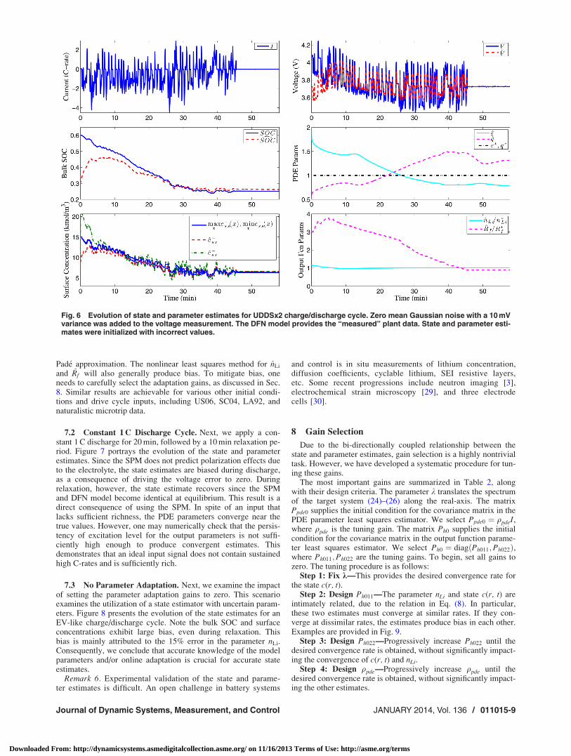
7.1 Electric Vehicle Charge/Discharge Cycle. First, weapply an electric vehicle-like charge/discharge cycle. This inputsignal is generated from two concatenated UDDS drive cyclessimulated on the models developed in Ref. [28]. This signal is ahighly transient input with large magnitude C-rates, thereby pro-ducing a sufficiently rich signal for parameter estimation. Figure 6portrays the evolution of the state and parameter estimates. Thestate estimates are represented by the bulk SOC, defined inEq. (76), and surface concentrations.

dSOCðtÞ ¼ 3

c�s;max

ð1

0

r2c�s ðr; tÞdr (76)

The PDE parameter estimates e; q and output function parameterestimates nLi; Rf , which are normalized to one in Fig. 6, also con-verge near their true values. Indeed, one expects some estimationbias for such a nonlinear and complex model. An expected estima-tion bias exists in e and q due to the overparameterization of the



Pad�e approximation. The nonlinear least squares method for nLi

and Rf will also generally produce bias. To mitigate bias, oneneeds to carefully select the adaptation gains, as discussed in Sec.8. Similar results are achievable for various other initial condi-tions and drive cycle inputs, including US06, SC04, LA92, andnaturalistic microtrip data.

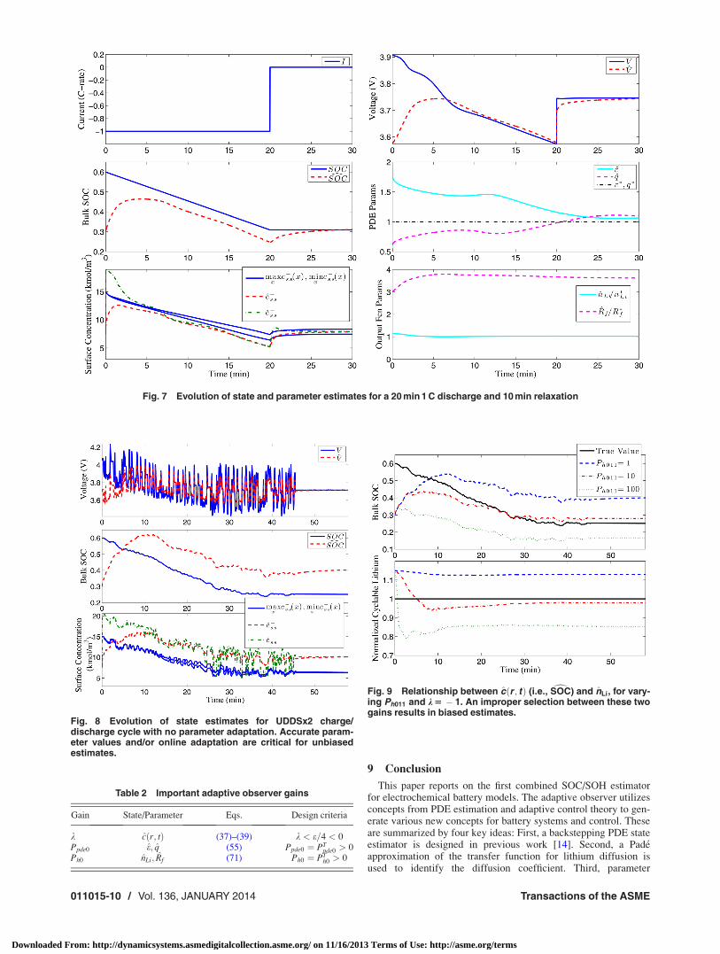
7.2 Constant 1 C Discharge Cycle. Next, we apply a con-stant 1 C discharge for 20 min, followed by a 10 min relaxation pe-riod. Figure 7 portrays the evolution of the state and parameterestimates. Since the SPM does not predict polarization effects dueto the electrolyte, the state estimates are biased during discharge,as a consequence of driving the voltage error to zero. Duringrelaxation, however, the state estimate recovers since the SPMand DFN model become identical at equilibrium. This result is adirect consequence of using the SPM. In spite of an input thatlacks sufficient richness, the PDE parameters converge near thetrue values. However, one may numerically check that the persis-tency of excitation level for the output parameters is not suffi-ciently high enough to produce convergent estimates. Thisdemonstrates that an ideal input signal does not contain sustainedhigh C-rates and is sufficiently rich.

7.3 No Parameter Adaptation. Next, we examine the impactof setting the parameter adaptation gains to zero. This scenarioexamines the utilization of a state estimator with uncertain param-eters. Figure 8 presents the evolution of the state estimates for anEV-like charge/discharge cycle. Note the bulk SOC and surfaceconcentrations exhibit large bias, even during relaxation. Thisbias is mainly attributed to the 15% error in the parameter nLi.Consequently, we conclude that accurate knowledge of the modelparameters and/or online adaptation is crucial for accurate stateestimates.

Remark 6. Experimental validation of the state and parame-ter estimates is difficult. An open challenge in battery systems

and control is in situ measurements of lithium concentration,diffusion coefficients, cyclable lithium, SEI resistive layers,etc. Some recent progressions include neutron imaging [3],electrochemical strain microscopy [29], and three electrodecells [30].

8 Gain Selection

Due to the bi-directionally coupled relationship between thestate and parameter estimates, gain selection is a highly nontrivialtask. However, we have developed a systematic procedure for tun-ing these gains.

The most important gains are summarized in Table 2, alongwith their design criteria. The parameter k translates the spectrumof the target system (24)–(26) along the real-axis. The matrixPpde0 supplies the initial condition for the covariance matrix in thePDE parameter least squares estimator. We select Ppde0 ¼ qpdeI,where qpde is the tuning gain. The matrix Ph0 supplies the initialcondition for the covariance matrix in the output function parame-ter least squares estimator. We select Ph0 ¼ diagðPh011;Ph022Þ,where Ph011;Ph022 are the tuning gains. To begin, set all gains tozero. The tuning procedure is as follows:

Step 1: Fix k—This provides the desired convergence rate forthe state c(r, t).

Step 2: Design Ph011—The parameter nLi and state c(r, t) areintimately related, due to the relation in Eq. (8). In particular,these two estimates must converge at similar rates. If they con-verge at dissimilar rates, the estimates produce bias in each other.Examples are provided in Fig. 9.

Step 3: Design Ph022—Progressively increase Ph022 until thedesired convergence rate is obtained, without significantly impact-ing the convergence of c(r, t) and nLi.

Step 4: Design qpde—Progressively increase qpde until thedesired convergence rate is obtained, without significantly impact-ing the other estimates.

Fig. 6 Evolution of state and parameter estimates for UDDSx2 charge/discharge cycle. Zero mean Gaussian noise with a 10 mVvariance was added to the voltage measurement. The DFN model provides the “measured” plant data. State and parameter esti-mates were initialized with incorrect values.



9 Conclusion

This paper reports on the first combined SOC/SOH estimatorfor electrochemical battery models. The adaptive observer utilizesconcepts from PDE estimation and adaptive control theory to gen-erate various new concepts for battery systems and control. Theseare summarized by four key ideas: First, a backstepping PDE stateestimator is designed in previous work [14]. Second, a Pad�eapproximation of the transfer function for lithium diffusion isused to identify the diffusion coefficient. Third, parameter

Fig. 9 Relationship between cðr ; tÞ (i.e., dSOC) and nLi, for vary-ing Ph011 and k 5 � 1. An improper selection between these twogains results in biased estimates.

Fig. 8 Evolution of state estimates for UDDSx2 charge/discharge cycle with no parameter adaptation. Accurate param-eter values and/or online adaptation are critical for unbiasedestimates.

Table 2 Important adaptive observer gains

Gain State/Parameter Eqs. Design criteria

k cðr; tÞ (37)–(39) k < e=4 < 0Ppde0 e; q (55) Ppde0 ¼ PT

pde0 > 0Ph0 nLi; Rf (71) Ph0 ¼ PT

h0 > 0

Fig. 7 Evolution of state and parameter estimates for a 20 min 1 C discharge and 10 min relaxation



sensitivity analysis is applied to elucidate the linear dependencebetween physically meaningful parameters related to capacity andpower fade. Fourth, an adaptive output function inversion tech-nique enables linear state estimation designs. Finally, we presentsimulations which demonstrate how the adaptive observer per-forms against a high-fidelity battery simulator—the Doyle-Fuller-Newman model. The composition of these unique ideas providesa combined SOC/SOH estimation algorithm for battery systemsusing electrochemical models.

A useful extension of the observer presented here is a state/parameter estimator for the DFN model. In particular, this wouldenable improved estimation accuracy at high C-rates. Moreover,the DFN model predicts additional SOH-critical variables, such asside reaction overpotentials. On-going work is also centeredaround output-feedback control schemes that utilize the presentedobserver to maximize energy/power while satisfying safe operat-ing constraints.

Nomenclature

A ¼ cell cross sectional area, m2

aj ¼ specific interfacial surface area, m2/m3

c0e ¼ Li concentration in electrolyte phase, mol/m3

cjs ¼ Li concentration in solid phase, mol/m3

cjss ¼ Li concentration at particle surface, mol/m3

cjs;max ¼ max Li concentration in solid phase, mol/m3

Djs ¼ diffusion coefficient in solid phase, m2/s3

F ¼ Faraday’s constant, C/molI ¼ input current, A

ij0 ¼ exchange current density, Vj ¼ positive (þ) or negative (�) electrode

kj ¼ reaction rate, A �mol1:5=m5:5

Lj ¼ electrode thickness, mnLi ¼ total number of Li ions, mol

q ¼ boundary input coefficient parameterR ¼ universal gas constant, J/mol-KRf ¼ lumped current collector resistance, XRj

s ¼ particle radius, mr ¼ radial coordinate, m, or m/mT ¼ cell temperature, Kt ¼ time, s

Uj ¼ equilibrium potential, VV ¼ output voltage, Vaj ¼ anodic/cathodic transfer coefficiente ¼ diffusion parameterej

s ¼ volume fraction of solid phase

References[1] Chaturvedi, N. A., Klein, R., Christensen, J., Ahmed, J., and Kojic, A., 2010,

“Algorithms for Advanced Battery-Management Systems,” IEEE ControlSystems Magazine, 30(3), pp. 49–68.

[2] Moura, S., Fathy, H., Callaway, D., and Stein, J., 2011, “A Stochastic OptimalControl Approach for Power Management in Plug-in Hybrid Electric Vehicles,”IEEE Trans. Control Syst. Technol., 19(3), pp. 545–555.

[3] Siegel, J. B., Lin, X., Stefanopoulou, A. G., Hussey, D. S., Jacobson, D. L., andGorsich, D., 2011, “Neutron Imaging of Lithium Concentration in LFP PouchCell Battery,” J. Electrochem. Soc., 158(5), pp. A523–A529.

[4] Liu, P., Wang, J., Hicks-Garner, J., Sherman, E., Soukiazian, S., Verbrugge,M., Tataria, H., Musser, J., and Finamore, P., 2010, “Aging Mechanisms ofLiFePO4 Batteries Deduced by Electrochemical and Structural Analyses,”J. Electrochem. Soc., 157(4), pp. A499–A507.

[5] Thomas, K., Newman, J., and Darling, R., 2002, Advances in Lithium-Ion Bat-teries, Mathematical Modeling of Lithium Batteries, Kluwer Academic/PlenumPublishers, New York, Chap. XII, pp. 345–392.

[6] Plett, G. L., 2004, “Extended Kalman Filtering for Battery Management Sys-tems of LiPB-Based HEV Battery Packs. Part 3. State and ParameterEstimation,” J. Power Sources, 134(2), pp. 277–292.

[7] Verbrugge, M., and Tate, E., 2004, “Adaptive State of Charge Algorithm forNickel Metal Hydride Batteries Including Hysteresis Phenomena,” J. PowerSources, 126(1–2), pp. 236–249.

[8] Verbrugge, M., 2007, “Adaptive, Multi-Parameter Battery State Estimator WithOptimized Time-Weighting Factors,” J. Appl. Electrochem., 37(5), pp.605–616.

[9] Hu, Y., and Yurkovich, S., 2012, “Battery Cell State-of-Charge EstimationUsing Linear Parameter Varying System Techniques,” J. Power Sources, 198,pp. 338–350.

[10] Santhanagopalan, S., and White, R. E., 2006, “Online Estimation of the State ofCharge of a Lithium Ion Cell,” J. Power Sources, 161(2), pp. 1346–1355.

[11] Domenico, D. D., Stefanopoulou, A., and Fiengo, G., 2010, “Lithium-IonBattery State of Charge and Critical Surface Charge Estimation Using anElectrochemical Model-Based Extended Kalman Filter,” ASME J. Dyn. Syst.,Meas., Control, 132(6), p. 061302.

[12] Smith, K. A., Rahn, C. D., and Wang, C.-Y., 2008, “Model-Based Electrochem-ical Estimation of Lithium-Ion Batteries,” 2008 IEEE International Conferenceon Control Applications, pp. 714–719.

[13] Klein, R., Chaturvedi, N. A., Christensen, J., Ahmed, J., Findeisen, R., andKojic, A., 2012, “Electrochemical Model Based Observer Design for aLithium-Ion Battery,” IEEE Trans. Control Syst. Technol., pp. 1–13.

[14] Moura, S. J., Chaturvedi, N., and Krstic, M., 2012, “PDE Estimation Techni-ques for Advanced Battery Management Systems—Part I: SOC Estimation,”Proceedings of the 2012 American Control Conference.

[15] Moura, S. J., Chaturvedi, N., and Krstic, M., 2012, “PDE Estimation Techni-ques for Advanced Battery Management Systems—Part II: SOH Identification,”Proceedings of the 2012 American Control Conference.

[16] Moura, S. J., Chaturvedi, N., and Krstic, M., 2012, “Adaptive PDE Observerfor Battery SOC/SOH Estimation,” 2012 ASME Dynamic Systems and ControlConference.

[17] Santhanagopalan, S., Guo, Q., Ramadass, P., and White, R. E., 2006, “Reviewof Models for Predicting the Cycling Performance of Lithium Ion Batteries,”J. Power Sources, 156(2), pp. 620–628.

[18] Newman, J., 2008, Fortran Programs for the Simulation of Electrochemical Sys-tems, University of California, Berkley, CA.

[19] Chen, C., 1998, Linear System Theory and Design, Oxford University Press,Inc., Oxford, UK.

[20] Krstic, M., and Smyshlyaev, A., 2008, Boundary Control of PDEs: A Courseon Backstepping Designs, Society for Industrial and Applied Mathematics,Philadelphia, PA.

[21] Delacourt, C., Poizot, P., Levasseur, S., and Masquelier, C., 2006, “Size Effectson Carbon-Free LiFePO4 Powders,” Electrochem. Solid-State Lett., 9(7), pp.A352–A355.

[22] Derrien, G., Hassoun, J., Panero, S., and Scrosati, B., 2007, “NanostructuredSn-C Composite as an Advanced Anode Material in High-Performance Lith-ium-Ion Batteries,” Adv. Mater., 19(17), pp. 2336–2340.

[23] Forman, J. C., Moura, S. J., Stein, J. L., and Fathy, H. K., 2012, “Genetic Identi-fication and Fisher Identifiability Analysis of the Doyle-Fuller-Newman ModelFrom Experimental Cycling of a LiFePO4 Cells,” J. Power, 210, pp. 263–275.

[24] Khalil, H. K., 2002, Nonlinear Systems, 3rd ed., Prentice Hall, EnglewoodCliffs, NJ.

[25] Ioannou, P., and Sun, J., 1996, Robust Adaptive Control, Prentice-Hall, Engle-wood Cliffs, NJ.

[26] Smyshlyaev, A., and Krstic, M., 2010, Adaptive Control of Parabolic PDEs,Princeton University, Princeton, NJ.

[27] Lund, B. F., and Foss, B. A., 2008, “Parameter Ranking by Orthogonaliza-tion—Applied to Nonlinear Mechanistic Models,” Automatica, 44(1), pp.278–281.

[28] Moura, S. J., Stein, J. L., and Fathy, H. K., 2012, “Battery-Health ConsciousPower Management in Plug-In Hybrid Electric Vehicles Via ElectrochemicalModeling and Stochastic Control,” IEEE Trans. Control Syst. Technol., 21,pp. 679–694.

[29] Morozovska, A., Eliseev, E., Balke, N., and Kalinin, S., 2010, “Local Probingof Ionic Diffusion by Electrochemical Strain Microscopy: Spatial Resolutionand Signal Formation Mechanisms,” J. Appl. Phys., 108(5), p. 053712.

[30] Fang, W., Kwon, O. J., and Wang, C.-Y., 2010, “Electrochemical-ThermalModeling of Automotive Li-Ion Batteries and Experimental Validation Using aThree-Electrode Cell,” Int. J. Energy Res., 34(2), pp. 107–115.



http://dx.doi.org/10.1109/MCS.2010.936293

http://dx.doi.org/10.1109/MCS.2010.936293

http://dx.doi.org/10.1109/TCST.2010.2043736

http://dx.doi.org/10.1149/1.3566341

http://dx.doi.org/10.1149/1.3294790

http://dx.doi.org/10.1016/j.jpowsour.2004.02.033



http://dx.doi.org/10.1007/s10800-007-9291-7



http://dx.doi.org/10.1115/1.4002475

http://dx.doi.org/10.1115/1.4002475


http://dx.doi.org/10.1149/1.2201987

http://dx.doi.org/10.1002/adma.200700748

http://dx.doi.org/10.1016/j.automatica.2007.04.006

http://dx.doi.org/10.1109/TCST.2012.2189773

http://dx.doi.org/10.1063/1.3460637

http://dx.doi.org/10.1002/er.1652

adaptive partial differential scott j. moura equation ...flyingv.ucsd.edu/papers/pdf/182.pdf ·...

Documents