adaptive filters chaptermwickert/ece5655/lecture_notes/arm/ece5655_chap8.pdf · chapter 8 •...

er

Adaptive FiltersIntroduction

The term adaptive filter implies changing the characteristic of afilter in some automated fashion to obtain the best possible signalquality in spite of changing signal/system conditions. Adaptivefilters are usually associated with the broader topic of statisticalsignal processing. The operation of signal filtering by definitionimplies extracting something desired from a signal containingboth desired and undesired components. With linear FIR and IIRfilters the filter output is obtained as a linear function of theobservation (signal applied) to the input. An optimum linear fil-ter in the minimum mean square sense can be designed to extracta signal from noise by minimizing the error signal formed bysubtracting the filtered signal from the desired signal. For noisysignals with time varying statistics, this minimization process isoften done using an adaptive filter.

For statistically stationary inputs this solution is known as aWiener filter.1

1.Simon Haykin, Adaptive Filter Theory, fourth edition, Prentice Hall, 2002.

WienerFilter

+

-

e n

y n

d n

x n

DesiredSignal

Observation

MMSEEstimateof d[n]

ErrorSignal

Chapt

8

ECE 5655/4655 Real-Time DSP 8–1

Chapter 8 • Adaptive Filters

Wiener Filter

• An M tap discrete-time Wiener filter is of the form

(8.1)

where the are referred to as the filter weights

– Note: (8.1) tells us that the Wiener filter is just an M-tapFIR filter

• The quality of the filtered or estimated signal is deter-mined from the error sequence

• The weights , are chosen such that

(8.2)

is minimized, that is we obtain the minimum mean-squarederror (MMSE)

• The optimal weights are found by setting

(8.3)

• From the orthogonality principle1 we choose the weightssuch that the error is orthogonal to the observations(data), i.e.,

1.A. Papoulis, Probability, Random Variables, and Stochastic Processes,third edition, McGraw-Hill, 1991.

y n wmx n m– m 0=

M 1–

=

wm

y n e n d n y n –=

wm m 0 1 M 1– =

E e2n E d n y n – 2 =

wm E e

2n 0 m 0 1 M 1– = =

e n

8–2 ECE 5655/4655 Real-Time DSP

Wiener Filter

(8.4)

– This results in a filter that is optimum in the sense of mini-mum mean-square error

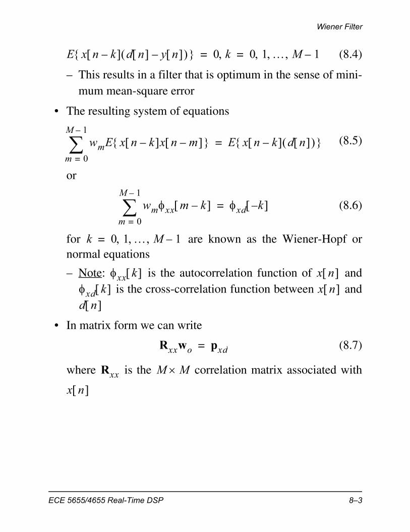
• The resulting system of equations

(8.5)

or

(8.6)

for are known as the Wiener-Hopf ornormal equations

– Note: is the autocorrelation function of and is the cross-correlation function between and

• In matrix form we can write

(8.7)

where is the correlation matrix associated with

E x n k– d n y n – 0 k 0 1 M 1– = =

wmE x n k– x n m– m 0=

M 1–

E x n k– d n =

wmxx m k– m 0=

M 1–

xd k– =

k 0 1 M 1– =

xx k x n xd k x n d n

Rxxwo pxd=

Rxx M M

x n



(8.8)

is the optimum weight vector given by

(8.9)

and is the cross-correlation vector given by

(8.10)

• The optimal weight vector is given by

(8.11)

• As a matter of practice (8.11) can be solved using sample sta-tistics, that is we replace the true statistical auto- and cross-correlation functions with time averages of the form

(8.12)

(8.13)

where N is the sample block size

Rxx

xx 0 xx M 1–

xx M– 1+ xx 0

= . . .

. . .

. . .

. . .

. . .

wo

wo wo0 wo1 woM 1–

T=

pxd

pxd xd 0 xd 1– xd 1 M– T

=

wo Rxx1–pxd=

xx k 1N---- x n k+ x n n 0=

N 1–

xd k 1N---- x n k+ d n n 0=

N 1–


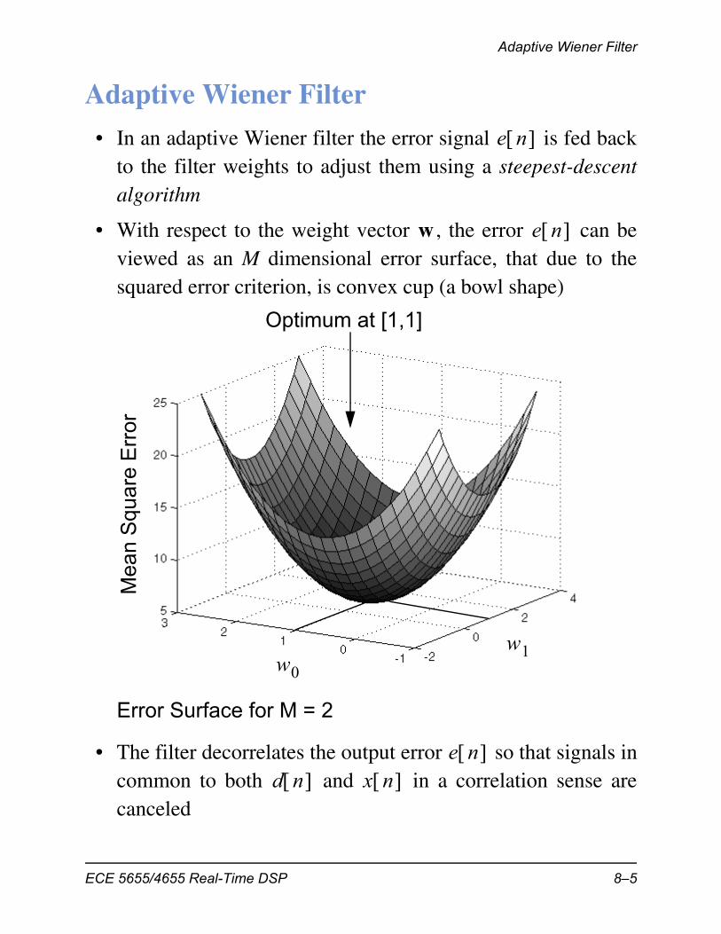
Adaptive Wiener Filter


• In an adaptive Wiener filter the error signal is fed backto the filter weights to adjust them using a steepest-descentalgorithm

• With respect to the weight vector , the error can beviewed as an M dimensional error surface, that due to thesquared error criterion, is convex cup (a bowl shape)

• The filter decorrelates the output error so that signals incommon to both and in a correlation sense arecanceled

e n

w e n

w0

w1

Mea

n S

quar

e E

rror

Optimum at [1,1]

Error Surface for M = 2

e n d n x n



• A block diagram of this adaptive Wiener (FIR) filter is shownbelow

Least-Mean-Square Adaptation

• Ideally the optimal weight solution can be obtained by apply-ing the steepest descent method to the error surface, but sincethe true gradient cannot be determined, we use a stochasticgradient, which is simply the instantaneous estimate of and from the available data, e.g.,

(8.14)

(8.15)

where

(8.16)

• A practical implementation involves estimating the gradientfrom the available data using the least-mean-square (LMS)algorithm

+

-

e n

y n

d n

x n

DesiredSignal

Observation

MMSEEstimateof d[n]

ErrorSignal

WienerFilter


AdaptiveAlgorithm

Rxxpxd

Rˆxx x n xT n =

pxd x n d n =

x n x n x n 1– x n M– 1+ T

=



• The steps to the LMS algorithm, for each new sample at timen, are:

– Filter to produce:

(8.17)

– Form the estimation error:

(8.18)

– Update the weight vector using step-size parameter :

(8.19)

• For algorithm stability, the step-size must be chosen suchthat

(8.20)

where

(8.21)

• In theory, (8.20) is equivalent to saying

(8.22)

where is the maximum eigenvalue of

x n

y n wm n x n m– m 0=

M 1–

wTn x n = =

e n d n y n –=

w n 1+ w n x n e n +=

0 2tap-input power--------------------------------------

tap-input power E x n k– 2 k 0=

M 1–

=

0 2max-----------

max Rxx



Adaptive Filter Variations1

• Prediction

• System Identification

• Equalization

1.B. Widrow and S. Stearns, Adaptive Signal Processing, Prentice Hall, NewJersey, 1985.

e n y n

d n

x n Delay Adaptive

Filter

s n

+-

e n y n

d n

x n

Plant

AdaptiveFilter

s n

+-

e n y n

d n

x n Plant/ Adaptive

Filter

s n

+-

Delay

++

Noise

Channel

TrainingPattern


Adaptive Line Enhancement

• Interference Canceling


• A relative of the interference canceling scheme shown above,is the adaptive line enhancer (ALE)

• Here we assume we have a narrowband signal (say a sinu-soid) buried in broadband additive noise

• The filter adapts in such a way that a narrow passband formsaround the sinusoid frequency, thereby suppressing much ofthe noise and improving the signal-to-noise ratio (SNR) in

e n y n

d n

x n Adaptive

Filter

+-

Signal +

Interference’

Interference

e n

y n x n – Adaptive

Filter

x n NB n BB n +=

z–

+

-

y n



Python ALE Simulation

• A simple Python simulation is constructed using a singlesinusoid at normalized frequency plus additivewhite Gaussian noise

(8.23)

• The SNR is defined as

(8.24)

def lms_ale(SNR,N,M,mu,sqwav=False): """ lms_ale lms ALE adaptation algorithm using an IIR filter. n,x,x_hat,e,ao,F,Ao = lms_ale(SNR,N,M,mu) *******LMS ALE Simulation************ SNR = Sinusoid SNR in dB N = Number of simulation samples M = FIR Filter length (order M-1) mu = LMS step-size mode = 0 <=> sinusoid, 1 <=> squarewave n = Index vector x = Noisy input x_hat = Filtered output e = Error sequence ao = Final value of weight vector F = Frequency response axis vector Ao = Frequency response of filter in dB ************************************** Mark Wickert, November 2014 """

# Sinusoid SNR = (A^2/2)/noise_var n = arange(0,N+1) # length N+1 if not(sqwav): x = 1*cos(2*pi*1/20*n) # Here A = 1, Fo/Fs = 1/20 x += sqrt(1/2/(10**(SNR/10)))*randn(N+1) else: # Squarewave case x = 1*sign(cos(2*pi*1/20*n)); # Here A = 1, Fo/Fs = 1/20 x += sqrt(1/1/(10**(SNR/10)))*randn(N+1) # Normalize mu mu /= M + 1

fo 1 20=

x n A 2fon cos w n +=

SNR A2

2w2

----------=



# White Noise -> Delta = 1, so delay x by one sample y = signal.lfilter([0, 1],1,x) # Initialize output vector x_hat to zero x_hat = zeros_like(x) # Initialize error vector e to zero e = zeros_like(x) # Initialize weight vector to zero ao = zeros(M+1) # Initialize filter memory to zero zi = signal.lfiltic(ao,1,y=0) # Initialize a vector for holding ym of length M+1 ym = zeros_like(ao) for k,yk in enumerate(y): # Filter one sample at a time x_hat[k],zi = signal.lfilter(ao,1,[yk],zi=zi) # Form the error sequence e[k] = x[k] - x_hat[k] # Update the weight vector ao = ao + 2*mu*e[k]*ym # Update vector used for correlation with e[k] ym = hstack((array(yk), ym[0:-1])) # Create filter frequency response F = arange(0,0.5,1/512) w,Ao = signal.freqz(ao,1,2*pi*F) Ao = 20*log10(abs(Ao)) return n,x,x_hat,e,ao,F,Ao

• A simulation is run using 1000 samples, dB, M =64, and

n,x,x_hat,e,ao,F,Ao = lms_ale(10,1000,64,0.005,False)

plot(n,e**2)#xlim([800,1000])ylabel(r'MSE')xlabel(r'Time Index n')title('SNR = 10 dB: Sinewave')grid();

SNR 10= 0.01 64=



plot(n,x)plot(n,x_hat)xlim([900,1000])legend((r'$x[n]$',r'$\hat{x}[n]$'),loc='best')ylabel(r'Input/Output Signal')xlabel(r'Time Index n')title('SNR = 10 dB: Sinewave')ylim([-1.5,1.5])grid();

Convergence Occursin Here (~275 samples)



plot(F,Ao)plot([0.05,0.05],[-40,0],'r')ylabel(r'Frequency Response in dB')xlabel(r'Normalized Frequency $\omega/(2\pi)$')title('SNR = 10 dB: Sinewave')grid();

• A C version of the above Python code will be very similarexcept all of the vector operations are replaced by for loops

Sinusoid Frequency



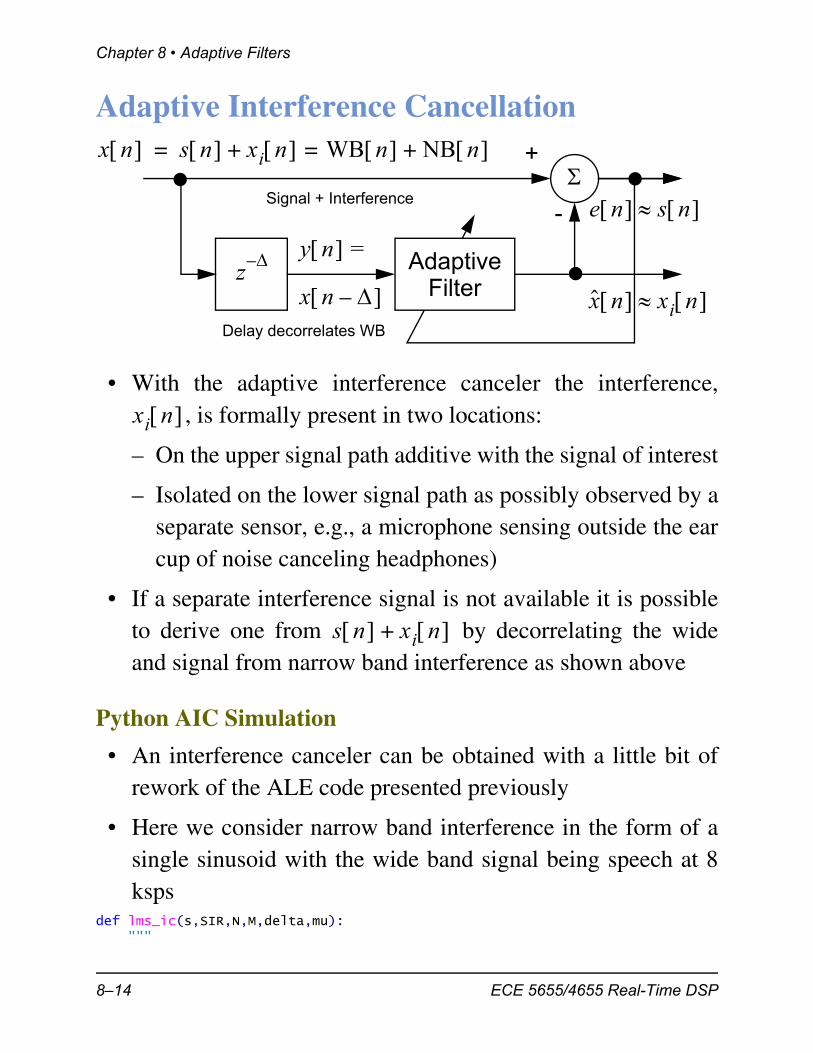
Adaptive Interference Cancellation

• With the adaptive interference canceler the interference,, is formally present in two locations:

– On the upper signal path additive with the signal of interest

– Isolated on the lower signal path as possibly observed by aseparate sensor, e.g., a microphone sensing outside the earcup of noise canceling headphones)

• If a separate interference signal is not available it is possibleto derive one from by decorrelating the wideand signal from narrow band interference as shown above

Python AIC Simulation

• An interference canceler can be obtained with a little bit ofrework of the ALE code presented previously

• Here we consider narrow band interference in the form of asingle sinusoid with the wide band signal being speech at 8ksps

def lms_ic(s,SIR,N,M,delta,mu): """

e n s n

x n – Adaptive

Filter

x n s n xi n + WB n NB n +==

z–

+

-Signal + Interference

Delay decorrelates WB

y n =

x n xi n

xi n

s n xi n +


Adaptive Interference Cancellation

Adaptive interference canceller using LMS and FIR n,x,x_hat,e,ao,F,Ao = lms_ic(s,SIR,N,M,delta,mu) *******LMS Interference Cancellation Simulation************ s = Input speech signal SIR = Speech signal power to sinusoid interference level in dB N = Number of simulation samples M = FIR Filter length (order M-1) delta = Delay used to generate the reference signal mu = LMS step-size n = Index vector x = Noisy input x_hat = Filtered output e = Error sequence ao = Final value of weight vector F = Frequency response axis vector Ao = Frequency response of filter ************************************** Mark Wickert, November 2014 """

# Input signal SIR = var(s)/(A^2/2) n = arange(0,N+1) # actually length N+1 x_i = cos(2*pi*1/20*n) # Here A = 1, Fo/Fs = 1/20 s = s[:N+1] # the input speech vector truncated to the length N+1 Ps = var(s) #estimate the AC power in s x = s + sqrt(2*Ps*10**(-SIR/10))*x_i # Form the reference signal y via delay delta y = signal.lfilter(hstack((zeros(delta), [1])),1,x) # Initialize output vector x_hat to zero x_hat = zeros_like(x) # Initialize error vector e to zero e = zeros_like(x) # Initialize weight vector to zero ao = zeros(M+1) # Initialize filter memory to zero zi = signal.lfiltic(ao,1,y=0) # Initialize a vector for holding ym of length M+1 ym = zeros_like(ao) for k,yk in enumerate(y): # Filter one sample at a time x_hat[k],zi = signal.lfilter(ao,1,array([yk]),zi=zi) # Form the error sequence e[k] = x[k] - x_hat[k] # Update the weight vector ao = ao + 2*mu*e[k]*ym # Update vector used for correlation with e[k] ym = hstack((array(yk), ym[0:-1])) # Create filter frequency response F = arange(0,0.5,1/512) w,Ao = signal.freqz(ao,1,2*pi*F) Ao = 20*log10(abs(Ao)) return n,x,x_hat,e,ao,F,Ao



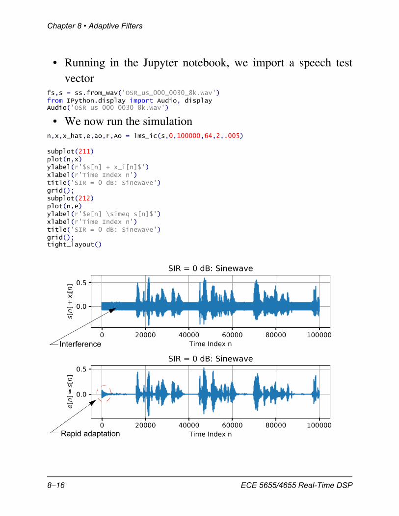
• Running in the Jupyter notebook, we import a speech testvector

fs,s = ss.from_wav('OSR_us_000_0030_8k.wav')from IPython.display import Audio, displayAudio('OSR_us_000_0030_8k.wav')

• We now run the simulationn,x,x_hat,e,ao,F,Ao = lms_ic(s,0,100000,64,2,.005)

subplot(211)plot(n,x)ylabel(r'$s[n] + x_i[n]$')xlabel(r'Time Index n')title('SIR = 0 dB: Sinewave')grid();subplot(212)plot(n,e)ylabel(r'$e[n] \simeq s[n]$')xlabel(r'Time Index n')title('SIR = 0 dB: Sinewave')grid();tight_layout()

Rapid adaptation

Interference


Cortex-M4 Implementation

Cortex-M4 Implementation

• The CMSIS-DSP library contains adaptive LMS filters


Adaptive Line Enhancer and Interference Cancellor on the FM4

• The next steps are to develop some examples using customcode and using the CMSIS-DSP library for comparison


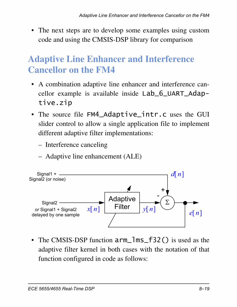
• A combination adaptive line enhancer and interference can-cellor example is available inside Lab_6_UART_Adap-tive.zip

• The source file FM4_Adaptive_intr.c uses the GUIslider control to allow a single application file to implementdifferent adaptive filter implementations:

– Interference canceling

– Adaptive line enhancement (ALE)

• The CMSIS-DSP function arm_lms_f32() is used as theadaptive filter kernel in both cases with the notation of thatfunction configured in code as follows:

e n y n

d n

x n Adaptive

Filter

+-

Signal1 +

Signal2

Signal2 (or noise)

or Signal1 + Signal2delayed by one sample



(8.25)

(8.26)

(8.27)

(8.28)

d n

left_in_sample P_vals[0] right_in_sample P_vals[1],+

P_vals[3] = 0

left_in_sample P_vals[0] noise P_vals[1],+

P_vals[3] = 1

x n left_in_sample, P_vals[4] = 0

d n 1– , P_vals[4] = 1

y n left_output_sample

e n right_out_sample

Change app with Filter Path = P_vals[3]



• For the interference canceling scenario the input is aversion of just interference portion of which is com-posed of both the desired signal plus the interference

• For the adaptive line enhancer the input is a copy of delayed by one sample

• Delaying by one sample uncorrelates the broadbandcomponent of from itself, meaning that the adaptive fil-ter will be ignoring this input

• The outputs for both algorithms need some interpretation too:

– With the interference canceler the error signal shouldcontain the desired signal with the interference removed

– For the ALE the broadband component, e.g., noise orspeech, is returned on and the narrowband compo-nent is recovered on

• Main module code listing:// fm4_adaptive_intr_GUI.c

#include "fm4_wm8731_init.h"#include "FM4_slider_interface.h"

int32_t rand_int32(void); // prototype for random number generator

// Create (instantiate) GUI slider data structurestruct FM4_slider_struct FM4_GUI;

//CMSIS-DSP adaptive filter structurearm_lms_instance_f32 LMS1;//arm_lms_norm_instance_f32 LMS1;uint16_t Ntaps = 100;float32_t a_coeff[100];float32_t states[100];float32_t mu = 1e-13;

float32_t x_inter, x_noise, x_speech;float32_t y, y_hat, error;float32_t y_del = 0.0f;

x n d n

x n d n

d n d n

e n

e n y n



void PRGCRC_I2S_IRQHandler(void) { union WM8731_data sample; //int16_t xL, xR;

gpio_set(DIAGNOSTIC_PIN,HIGH); // Get L/R codec sample sample.uint32bit = i2s_rx();

// Map L & R inputs to adaptive filter variable names x_noise = (float32_t)(((short)rand_int32())>>2); x_inter = (float32_t)sample.uint16bit[LEFT]; x_speech = (float32_t)sample.uint16bit[RIGHT]; if (FM4_GUI.P_vals[3] < 1) {

// Used for interference cancellery = FM4_GUI.P_vals[0]*x_inter + FM4_GUI.P_vals[1]*x_speech;

} else { // Used for ALE (note noise is generated internally)

y = FM4_GUI.P_vals[0]*x_inter + FM4_GUI.P_vals[1]*x_noise; } if (FM4_GUI.P_vals[3] < 1) // For interference cancelling { // input/src ref output error blk size arm_lms_f32(&LMS1, &x_inter, &y, &y_hat, &error, 1); } else // ALE where input is tone + noise { // input/src ref output error blk size

arm_lms_f32(&LMS1, &y_del, &y, &y_hat, &error, 1); } //arm_lms_norm_f32(&LMS1, &y_del, &y, &y_hat, &error, 1); y_del = y; // update one sample delayed version of the reference input

// Return L/R samples to codec via C union sample.uint16bit[LEFT] = (int16_t) y_hat; sample.uint16bit[RIGHT] = (int16_t) error; i2s_tx(sample.uint32bit);

NVIC_ClearPendingIRQ(PRGCRC_I2S_IRQn);

gpio_set(DIAGNOSTIC_PIN,LOW);}

int main(void){ // Initialize the slider interface by setting the baud // rate (460800 or 921600) // and initial float values for each of the 6 slider parameters

init_slider_interface(&FM4_GUI,460800, 1.0, 1.0, 1.0, 1.0, 0.0, 0.0);



// Send a string to the PC terminal write_uart0("Hello FM4 World!\r\n");

// Initialize LMS arm_lms_init_f32(&LMS1,Ntaps,a_coeff,states,mu,1); //arm_lms_norm_init_f32(&LMS1,Ntaps,a_coeff,states,mu,1);

// Some #define options for initializing the audio codec interface: // FS_8000_HZ, FS_16000_HZ, FS_24000_HZ, FS_32000_HZ, FS_48000_HZ, // FS_96000_HZIO_METHOD_INTR, IO_METHOD_DMA // WM8731_MIC_IN, WM8731_MIC_IN_BOOST, WM8731_LINE_IN fm4_wm8731_init (FS_48000_HZ, // Sampling rate (sps)

WM8731_LINE_IN, // Audio input port IO_METHOD_INTR, // Audio samples handler WM8731_HP_OUT_GAIN_0_DB, // Output hphone jack Gain (dB) WM8731_LINE_IN_GAIN_0_DB); // Line-in input gain (dB)

while(1){// Update slider parametersupdate_slider_parameters(&FM4_GUI);// Update LMS mu if slider parameter changesif(FM4_GUI.P_idx == 2){ mu = FM4_GUI.P_vals[2]*1e-13f;

arm_lms_init_f32(&LMS1,Ntaps,a_coeff,states,mu,1);}

}}

int32_t rand_int32(void){ static int32_t a_start = 100001;

a_start = (a_start*125) % 2796203; return a_start;}

• Capture some screen-shots of the running application



• ALE - fully adapted

• AIC - fully adapted

Narrow band ouput (blue): y[n]

Wide band ouput (orange): e[n]

339 Hz tone with noise reduced

Signal of interest 3.1kHz tone (orange): e[n]

Interfering 339 Hz tone (blue): y[n]

While adapting we see 339 Hztone in orange spectrum, butfalling


adaptive filters chaptermwickert/ece5655/lecture_notes/arm/ece5655_chap8.pdf · chapter 8 •...

Documents