ad-a269 684 - defense technical information center · ad-a269 684 control and ocean ... 1991). in...
TRANSCRIPT

Naval Command. AD-A269 684Control and Ocean San Diego, CA ll 111 11111Surveillance Center RDT&E Division 92152-5001
Technical Report 1571
January 1993
Evaporation DuctCommunication:Measurement Results
L. T. RogersK. D. Anderson
DTICELECTE
SE21993Uv E D~
AApproved for public release; distribution is unlemiterf
2197 1

Technical Report 1571
January 1993
Evaporation Duct Communication:Measurement Results
Acceslon ForL T. Rogers 4nTIS CRA&I
K. D. Anderson }DTIC TABUnannounced 0Justification .......................
By ..........Distribution I
Availability Codes
Avail and/orDist Special
.lIj

NAVAL COMMAND, CONTROL ANDOCEAN SURVEILLANCE CENTER
RDT&E DIVISIONSan Diego, California 92152-5001
J. D. FONTANA, CAPT, USN R. 1. SHEARERComm, anding Officer Executive Director
ADMINISTRATIVE INFORMATION
Work for this report was performed by the Tropospheric Branch, Code 543, in theOcean and Atmospheric Sciences Division, Research, Development, Test and Evalua-tion Division (NRaD) at the Naval Command, Control and Ocean Surveillance Center(NCCOSC), San Diego, California 92152-5001, during the period of FY 91 - FY 93.The work was funded by the Office of the Chief of Naval Research, program element0602232N, project number RC32WI 1.
Released by Under authority ofR. A. Paulus, Head J, H. Richter, HeadTropospheric Branch Ocean and Atmospheric
Sciences Division
RV
EXECUTIVE SUMMARY
OBJECTIVES
The Evaporation Duct Communication (EDCOM) project evaluates an alternativeship-to-ship communication channel that exploits the natural environment. It is a uniqueproject using a microwave communication circuit (similar to the commercial line-of-sight[LOS] microwave links that carry voice and data across the country) on an over-water.over-the-horizon (OTH) path where successful communication depends on the evaporationduct. A one-way 83-km transmission path is instrumented to simultaneously measure sur-face meteorological conditions and radio frequency (RF) characteristics of the communica-tion channel. Received Signal Levels (RSL) measurements are compared to propagationmodel RSL predictions that are based on knowledge of the surface meteorology. PercentError-Free Seconds (%EFS), Bit-Error Rate (BER) and other industry standard parame-ters of digita1knik pcrfoi,-i,. measured at DS-i transmission ateis (i.544 tisegdbitsper second). These measurements are used to validate and to improve the propagationmodels so that the performance of similar communication circuits can be predicted fromknowledge of the environmental conditions.
RESULTS
The principal results of the EDCOM project are as follows:
1. First, EDCOM has provided experimental data to assess the validity of a propaga-tion model used for the development and design of an alternative Super High Frequency(SHF) link for U.S. Navy ship-to-ship communications.
2. EDCOM has demonstrated the reliability of an OTH communication link thatdepends on the evaporation duct for successful link operation.
3. EDCOM has provided statistics required for optimal code design for the digital link.
RECOMMENDATIONS
1. The low percentage of successful communications (about 25%) strongly suggeststhat the development and design of a SHF link focus on a system that does not rely on theevaportion duct for enhanced communication capabilities. It is recommended that the SHFlink be designed for LOS ranges where availabilities of 99.99% or better can be achieved.
2. It is recommended that the frequency selection for a LOS system consider evapora-tion ducting effects. Communication to ranges of twice LOS for lower frequency (I to 5GHz) systems will occur infrequently; whereas, for higher frequency (5 to 14 Gliz) systems,twice LOS ranges are observed about 25% of the time.
3. It is recommended that further studies be made to optimize signal coding and proto-col procedures during bursty channel conditions.
' . i i I iI
CONTENTS
INTRO D UCTIO N ................................... ............. I
METEOROLOGICAL AND PROPAGATION MODELS ........... 4
RECEIVE SITE INSTRUMENTATION .......................... 6
TRANSMIT SITE INSTRUMENTATION ......................... 8
INSTRUMENT SCHEDULING ................................. 8
TRANSMITTER AND RECEIVER TESTING .................... 9
ANTENNA TESTING ......................................... 11
LOSS CALCULATIONS ........................................ 12
R E SU LT S ......................................................... 14
SOUTHERN CALIFORNIA COASTAL CLIMATE ................ 17
LONG-TERM TIME SERIES ................................... 17
CUMULATIVE DISTRIBUTIONS ............................... 33
HIGH SPEED TESTS .......................................... 41
DIGITAL SYSTEM PERFORMANCE ........................... 50
CO N CLU SIO N S ................................................... 51
R EFER EN CES .................................................... 52
FIGURES
1. Southern California coastline showing EDCOM transmission path andtransm itter and receiver horizons .................................. 1
2. Transmit site equipment showing digital transmission test sets (top)and transm itters (bottom ) . ....................................... 2
3. Transmit site at San Mateo Point, California ......................... 3
4. Receive site at building 599, NCCOSC RDT&E facility,San D iego, California ............................................ 4
5. Receive site functional diagram . .................................. 7
6. 7.5-GHz system testing arrangement ............................... 10
7. Receiver calibration curves . ...................................... 11
8. Montgomery field atmospheric soundings from 8 January 1992through 23 February 1992. Each abscissa division is 25 M-units .......... 15
9. Montgomery field atmospheric soundings from 23 February 1992through 26 March 1992. Each abscissa division is 25 M-units ............ 16
iii

10. Legend for time series in figures 11 through 22 ...................... 18
11. Time series covering 28 January 1992 through 31 January 1992 .......... 19
12. Time series covering 1 February 1992 through 4 February 1992 .......... 20
13. Time series covering 5 Februaiy 1992 through 8 February 1992 .......... 2114. Time series covering 9 February 1992 through 12 February 1992 ........ 2215. Time series covering 13 February 1992 through 16 February 1992 ...... 23
16. Time series covering 17 February 1992 through 20 February 1992 ........ 24
17. Time series covering 22 February 1992 through 25 February 1992 ........ 25
18. Time series covering 29 February 1992 through 3 March 1992 .......... 26
19. Time series covering 2 F March 1992 through 14 March 1992 ............ 2719. Time series covering 15 March 1992 through 14 March 1992............ 28
20. Time series covering 15 March 1992 through 18 March 1992 ............ 28
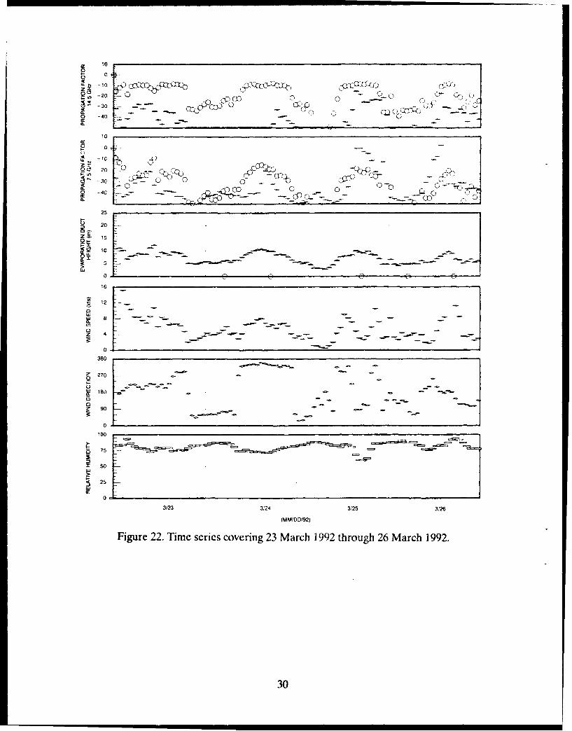
21. Time series covering 19 March 1992 through 22 March 1992 ............ 2922. Time series covering 23 March 1992 through 26 March 1992 ............ 30
23. Cumulative distributions of climatology predicted, meteorologicalmeasurement predicted and measured propagation factors ............ 34
24. Cumulative distribution of percent error free seconds (17 EFS) .......... 35
25. Cumulative distribution for meteorological measurement predictedand measured propagation factor for onshore flow ................... 36
26. Propagation factor versus evaporation duct height for hour averagedpropagation factors. The solid lines are model predictions based uponneutral evaporation duct profiles . ................................. 37
27. Propagation factor versus evaporation duct height separating surfaceand elevated duct observations (triangles) from purely evaporativeducting cases. The solid lines are model predictions based uponneutral evaporation duct profiles . ................................. 39
28. Propagation factor versus evaporation duct height from purelyevaporative ducting cases with linear least squares fit lines forevaporation duct heights between 9 and 17 meters. Unmarked solidlines on each graph are model predictions based upon neutralevaporation duct profiles ......................................... 40
29. 1-Hz sampling of 250-second time series of I500T, 9 February 1992.Evaporative ducting is dominant mode of propagation ................ 42
30. 1 -Hz sampling of 250-second time series of 1500T, 24 February 1992.A surface based duct is the dominant mode of propagation ............ 43
31. Distribution and density of difference between 1-Ilz samples andmean value of 250-second time series of propagation factors wherethe evaporation duct is the dominant mode of propagation ............. 44
iv

32. Distribution and density of difference between 1-Hz samples andmean value of 250-second time series of propagation factors wherethe evaporation duct is not the dominant mode of propagation .......... 45
33. One-second interval sampling of propagation factor and bit-errorrate of 14.5-GViz signal at 1500T on 3 March 1992 .................... 46
34. One-second ii~terval sampling of propagation factor and bit-errorrate of 7.5-GHz signal at 1500T on 17 February 1992 .................. 47
35. 20-Hz sample rate time series of propagation factors taken 21 July 1992. 48
36. Power spectrum from series of nine, 4096-point, 20-Hz sample ratetim e series of 21 July 1992 . ................................. ..... 49
37. Scatter plot of percent error-free seconds (%EFS) versuspropagation factor . ............................................. 50
TABLES
1. Percentage occurrences for surface-based and elevated ducts inSan D iego, C alifornia ............................................ 5
2. A nalog input channels . .......................................... 7
3. Receive digital signal quality measurements ......................... 8
4. Loral Terracom transmitter and receiver rated and measuredspecifications . .................................................. 10
5. Antenna perform ance . .......................................... 12
6. Summary of system constants for 7.5-GHz and 14.5-GHz links .......... 12
7. Dates of measurements in 1992 .................................... 14
v

INTRODUCTION
This report provides results from an experiment testing the feasibility of using the evap-oration duct to support an alternative high-speed communication system for Navy applica-tions. The feasibility of this link was discussed in an earlier study (Anderson, 1991), andpreparation for the experiment, including software development and transmitter andreceiver site preparation, was documented in a progress report (Anderson and Rogers,1991). In this report, meteorological and RF propagation models are reviewed. Data fromthe EDCOM propagation experiment are summarized and are used to assess RF propaga-tion model predictions that are derived from climatology. EDCOM digital link perfor-mance statistics are presented and are related to actual and predicted average RSL values.Additionally, high-speed, time-series analysis is provided for code word and network proto-col design.
EDCOM simulates a realistic ship-to-ship communication link. Antenna heights aretypical of shipboard installations, as they are approximately 25 m above the ocean surface.This height corresponds to a 41.2-km line-of-sight (LOS) distance between transmit andreceive sites. The EDCOM path, between the transmitter at San Mateo Point and thereceiver in Point Loma, is 83.1 km in length, which is more than twice the LOS range. Amap of the southern California coastline from Point Loma (San Diego) to San Mateo Point(the northern coastal point of Camp Pendleton) is shown in figure 1. The figure shows bothtransmitter and receiver sites and their line-of-sight horizon.
TRANSMITTER
SAN MATEO 33 23'21"N 117'35'39"EPOINT % 25m ABOVE MEAN SEA LEVEL
TRANSMITTER %,HORIZON ,20.6 km
831 kmPATH
9.
REEE SAN DIEGORECEIVER • .
HORIZON20.6 km
POINT LOMARECEIVER32' 41' 47"N 117-15'14"E25m ABOVE MEANSEA LEVEL
Figure 1. Southern California coastline showing EDCOMtransmission path and transmitter and receiver horizons.
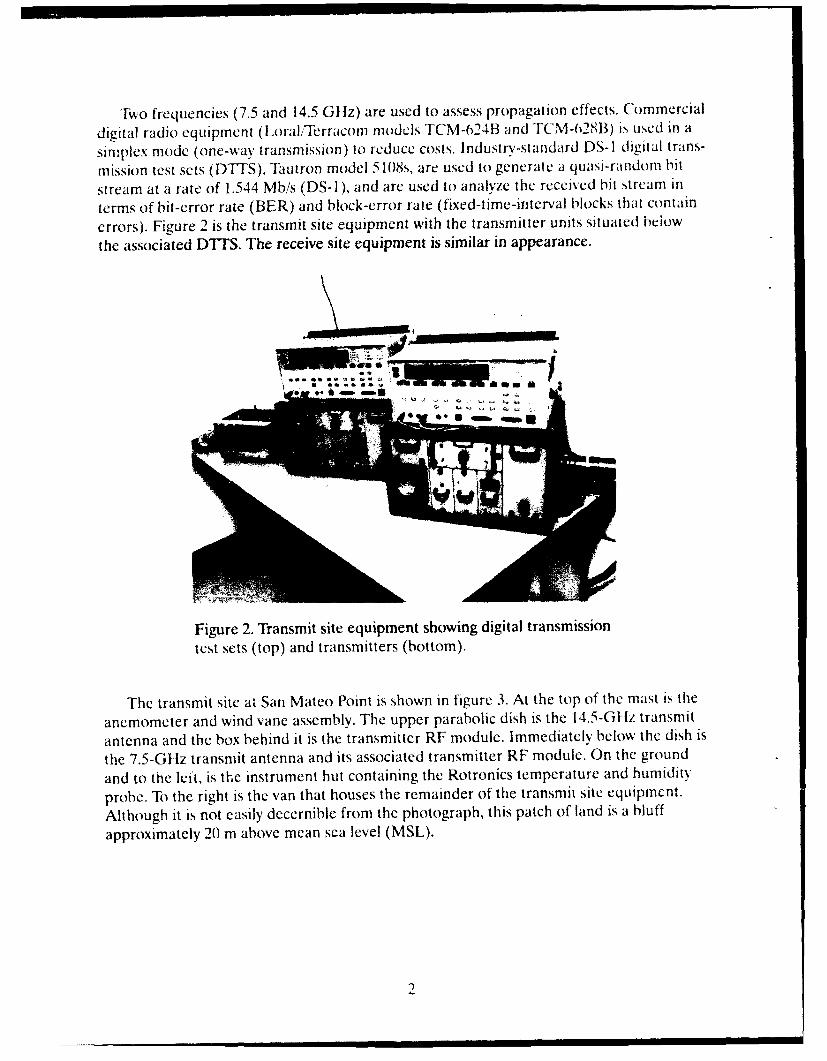
Two frequencies (7.5 and 14.5 061z) are used to assess propagation effects. Commercial
digital radio equipment (Loral,'Terracomr models TCM-624B and TCM-612813) is used in a
simplex mode (one-way transmission) to reduce costs. Industry-standard DS-I digital trans-
mission test sets (DTTS), Tautron model 5108s, are used to generate a quasi-random bit
stream at a rate of 1.544 Mbis (DS-1), and are used to analyze the received bit stream in
terms of bit-error rate (BER) and block-error rate (fixed-time-interval blocks that contain
errors). Figure 2 is the transmit site equipment with the transmitter units situated below
the associated DTTS. The receive site equipment is similar in appearance.
Figure 2. Transmit site equipment showing digital transmissiontest sets (top) and transmitters (bottom).
The transmit site at San Mateo Point is shown in figure 3. At the top of the mast is the
anemometer and wind vane assembly. The upper parabolic dish is the 14.5-GHz transmit
antenna and the box behind it is the transmitter RF module. Immediately below the dish is
the 7.5-Gtlz transmit antenna and its associated transmitter RF module. On the ground
and to the left, is the instrument hut containing the Rotronics temperature and humidity
probe. To the right is the van that houses the remainder of the transmit site equipment.
Although it is not easily decernible from the photograph, this patch of land is a bluff
approximately 20 m above mean sea level (MSL).
2I

Figure 3. Transmit site at San Mateo Point. California.
1li*'ureT J I"it hl r of the reCCNciv sitc lot alt d III Bulid rue 591 ait 111e N ('('()S(Ri)] I I[ It~ti SAn I ID IeTO. ( a11fvImnI, TI ']1 3nIns Ir ni ulII IIt huI I th R i Ir onc~l ) eme-
altir a nd huni11idi\ probe i to th flic h an111 1d at timc endL (it 11he pietý Ne h\1v-11r the:anemoflieterCM and \NindL vane onl a post. IXW mu ne,1-d s'Ce nSOFt tor nI1La-trementCII (11 se'A-
,u rt ace te mperatutre arc 11ou nie1d on1 theC pitII 11 mldi ii
I xpchrcim-il nii masuremnitts show that at t ui RS~I. enhanicementts (Iin (M), due to e poral mio det ictrig. arc rou gl-T 0I ýC thepit I-CI Ittd h\ t Iimatoh g'ieal-b e rpgtoruodels for hoth1 7.5ý and 14.5ý (d i. 1(SI cxcoe , tdsihe In'r1SU11COP an ICI\L urecedsignal, IC\ e:l(I RSL ) ruiredtl-c. for -':rror-41ree commuitnication 2-7' ojt thj tIe a1Ct 14.45 (' l/I. anI4'0
the time ac ;t 7 TO (iIz. 1 hei chaI-nnel is a, hurmtv e hannln Re Litli, el maill a mini tiits (t pi c x I
le'Ss than 5" LIM Mr reqiredMIC to go from- 0 ~(' erirol ree- sconids ( IA'S) to 90I (i 05 F. I -Sasl meaitsuired over 5-mlinutet intervals. Substantialk lx ore power is' iequired to atchieve 99
LIFS.

ProI
Figure 4. Receive site at building 599, NCCOSC RDT&E facility,San Piego. Callfornil.
M L:TE( ROLO(;IC., X NI) PROPAGATFION NIOI)ELS
*Vhei C\ aporation duict has been rccopilitcd for Many yewars is a ropasaI lionl phicnonie-
non that can Increase heonrd-hlorlion radi-io signals 11v many d B3s ahoke di ft ract 'ion tic id
lex cis for frcequen~cis above 2-G (i 0 /( itncv. et al.. I 985 ). ihirhlentim mixing, in thle ur~taicc
lave r ( :ir- Sca hoiinda rv) causesa rapid decrease in thec wat r-vaipo 'iContent of tile ar.
x\ hich, in turn, craites, a ton egtv radio ret'ract ivit\ gradient that formis an cx apora-
tive duitct. Ti duct acts as a leakv waive guide. Ani RI' signal canl propagate withl ai 11\\
atIc ntUiMon rate w\ithll tinlte guide that3 IS houndedI 11V the Sea surface and thle cx apol Irtit in
duict lici ght . At mrani.es beyond thle normal radio horiion. tihe field St rength in thle duict max.
bc I10 to 1 00 d13B greater than thle diffraction field strength. Abovc thle duct. til h: h feld
strenvth deere ases rapidly: hiowever, duie ito leakage from the duct. the Signal strengths mia-'
still be s'l l'st ant ialk- hligher than (the diffract ion field. The Signal enhandrcemenrt depen'ds
strongly onl fre qucencv because thecse ducts arc x erticallx tin1, t\pi)cali\ less than 2)ill.
In pratctice. boundair\-laver tlh ii'v\ rel ates bu'lk suirface nietcoroh'gicial mecasuiremenits ot
air tempelratureC. seal temiperature. wind spe~d. and hum toile eVaplorationl duet height.[vaporat ion duict hei glOi t Is co'mputed using, the .lcskc (I Q71) model as imp11lenienll~e h\
I~ ~ Iine 17)wtthrastbltmoiications suggeted1 -uu1IOS) nate
mal11 lx neutrall ilrt is)phe rC (k where the: aitr- Seal temlperature di t1*1Ie reC nec -s/e ) the mo dified
refract ivit\ prot'iti .1(z ) IS
4

M(z) M(0) + 0.125(z - (6 + zo))In[(z + zo)/zo) (1)
where z is height above the ocean, 0 is evaporation dl,:t height, and z-ý is a length charac-terizing boundary roughness,
Numerical propagation modeling techniques agree with RF measurement results whensingle-station surface meteorological obsc!vations a.re available to determine the refractiv-itv-versus-altitudc profile of the cvaporakion duct (K.itzin, Bauchman and Binnian. 1947;Richter and ttitney, 1988; Anderson, 1990). When the atmospheric refractivity profileabove the evaporation duct height is a standard profile (M(z) is monotonically decreasing ata rate of 118 Mlkim), the evaporation duct is the dominant mode of propagation. Nonstan-dard atmospheric refractivity profiles, particularly surface-based ducts, can raise receivedsignal levels beyond LOS ranges several dB's above free-space levels, often 20 dB or moreabove the already enhanced signal levels that are seen when there is a standard refractivityprofile above the evaporation duct height. When the refractivity profile above the evapora-tion duct height is neither standard nor nearly so, the evaporation duct may not be thedominant propagation mode. In the San Diego area, where the EDCOM experiment tookplace. nonstandard atmospheric refractivity profiles (which include surface-based and clc-vatcd ducts) are common. Table I provides percentages of soundings that indicate the pres-cnce of surface-based and elevated ducts in the San Diego area (Patterson. 19887). Of the86 atmospheric soundings taken at Montgomery field in San Diego during the EDCOMexperiment, only 53 (62%) show standard or nearly standard refractivity profiles. To vali-date the model for predicting the usefulness of the evaporation duct as an alternative com-munications channel, it is therefore necessary to separate RSL data that are associated wvithstandard atmospheric refractivity profiles above the evaporation duct height from thosethat are not.
Table 1. Percentage of occurrences for surface-based and elevated ducts in San Diego. CA.
Month/Ii Occurrence
Duct Type Jan Feb Mar Apr May Avg. (,)
Surface-based Ducts
Day 18 18 20 17 18 18.2
Night 24 24 18 14 11 8.2
Elevated Ducts
Day 27 27 31 41 48 34.8
Night 39 39 44 55 73 50).0
The waveguide propagation model, known as MLA YER, was originally developed byBaumgartner (1983) and was briefly described by Ilitney, et al. (1I985). ML4 YER, based onthe formalism developed by Budden (1961). solves the modal equation for an arbitrary
5
vertical, multiple-linear-segment refractivity profile using a root-finding scheme thatlocates all modes with attenuation rates less than a specified value. Surface roughness isaccounted for by modifying the surface-reflection coefficient, which is based on the windspeed. Horizontal homogeneity of refractive conditions is assumed.
Measurements of ambient air temperature, sea temperature, wind speed. and relativehumidity are used to calculate the evaporation duct hcight 0. Equation I is used to calcu-late the vertical refractivity profile M(z) that is needed by the MELAYER program. Mca-sured wind speed is used to calculate the surface roughness parameter (. which is also usedby MLA YER.
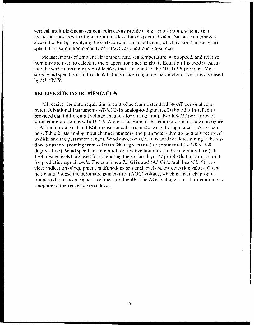
RECEIVE SITE INSTRUMENTATION
All receive site data acquisition is controlled from a standard 386AT personal com-puter. A National Instruments AT-MIO-16 analog-to-digital (A,'I)) board is installed toprovided eight differential voltage channels for analog input. Two RS-232 ports provideserial communications with D'ITS. A block diagram of this configuration is shown in figurc5. All meteorological and RSL measurements are made using the eight analog A 1) chan-nels. Table 2 lists analog input channel numbers, the parameters that are actually recordedto disk, and the parameter ranges. Wind direction (Ch. 0) is used for determining if ithe air-flow is onshore (coming from = 160 to 340 degrees true) or continental (z 340 to IN){tdegrees true). Wind speed, air temperature. relative humidity, and sea temperature (Ch1 -4, respectively) are used for computing the surface layer M profile that, in turn, is usedfor predicting signal levels. The comhined 7.5 G1 1z and 14.5 GI 1z fault bus (Ch. 5) pro-vides indication of e-quipment malfunctions or signal levels below detection values. ('han-nels 6 and 7 sense the automatic gain control (AGC) voltage, which is inverselv propor-tional to the received signal level measured in dB. The AGC voltage is used for continuoussampling of the received signal level.
6

- WIND DIRECTIONS (CH 0)WIND SPEED (CH 1) /
SAIR TEMPERATURE (CH 2)SRELATIVE HUMIDITY (CH 3)
SEA TEMPERATURE (CH 4)GHzS 14.5 GHz FAULT BUS (CH 5) PARABOLIPARABOLIC
7,5 GHz FAULT BUS (CH ANTENNA7.5 GHz AGC (,CH 6) ,
7 5 GHzPARABOLICANTENNA
LORAL LORAL ALTPORTTCM 624B TCM 628A
SIGNAL RECEIVER RECEIVERSCALING 7.5 GHz 14.5 GHz
COMBININGCKTS
ANALOG TDIIGITA
RECIV SIE
TAUTRON TAUTRON TRANSMISSION5108 5108 TEST SETS
l I RS-232 SERIAL PORT
RS - 232 SERIAL PORT
II NATIONAL INSTRUMENTS MULTI-I
I AT-M{O- 16 Comm1 ANALOG TO DIGITAL 4 X RS232
BOARD BOARD
I RECEIVE SITE
38bAT PERSONAL COMPUTER
Figure 5. Receive site functional diagram.
Table 2. Analog input channels.
Ch. Parameter Parameter Range
0 Wind Direction 0 to 360 deg.
I Wind Speed 0 to 86.8 knots
2 Air Temperature -20 to 55°C3 Relative Humidity 0 to 100 (11§ rh
4 Sea Temperature 0 to 100,C
5 Combined Fault Bus 0 to 4.5 v
6 7.5 (ii 1z AGC voltage + I to -4 v
7 14.5 G(3z AGC voltage +1 to -4 v
7
To comply with a maximum of 8 available analog channels, the 7.5 and 14.5 GHz faultbusses are combined by a voltage addition circuit in channel 5. Both channels 6 and 7 usescaling circuits (voltage divider networks) to divide the AGC voltages by a factor of 3 toreduce the signal within the range of the AiD board. All receiver testing and system opera-tion utilizes this configuration. (For the remainder of this paper, the term AGC voltagerefers to this divided signal.)
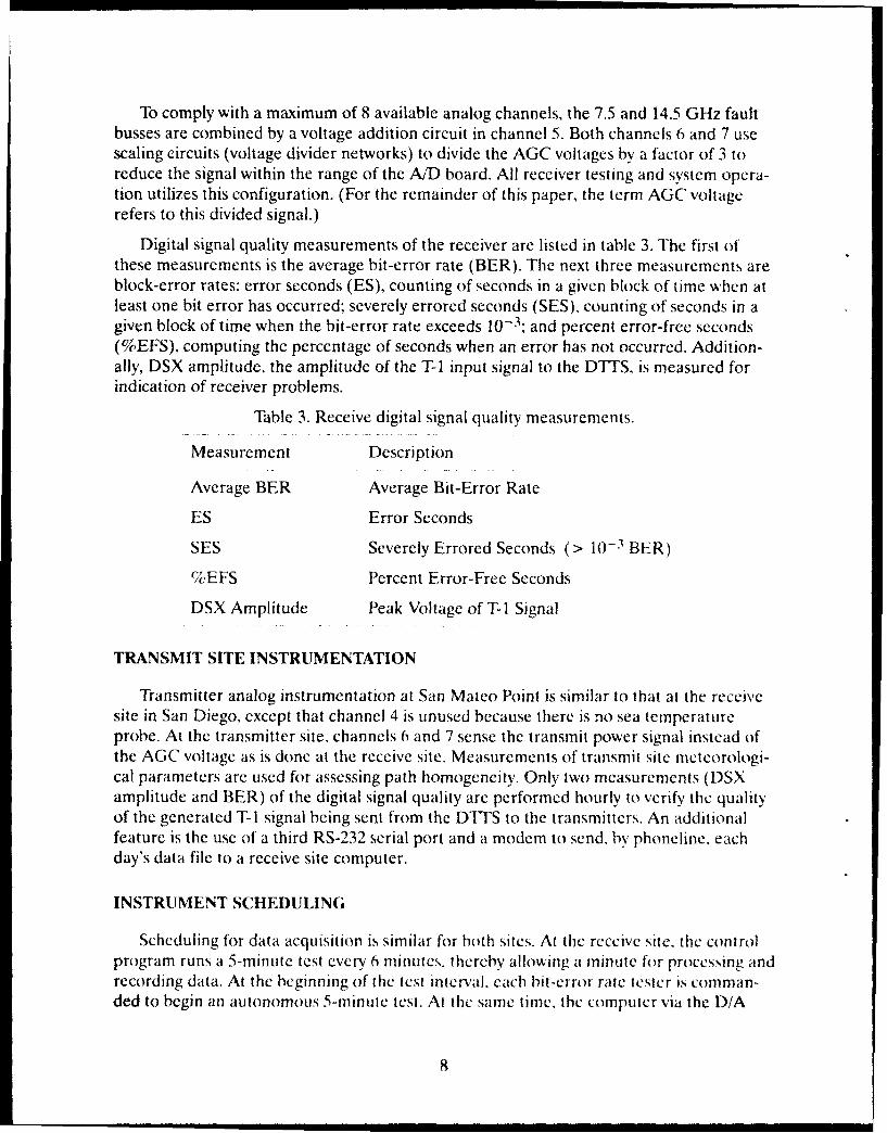
Digital signal quality measurements of the receiver are listed in table 3. The first ofthese measurements is the average bit-error rate (BER). The next three measurements areblock-error rates: error seconds (ES), counting of seconds in a given block of time when atleast one bit error has occurred; severely errored seconds (SES), counting of seconds in agiven block of time when the bit-error rate exceeds 10-3; and percent error-free seconds(%EFS), computing the percentage of seconds when an error has not occurred. Addition-ally, DSX amplitude, the amplitude of the T-1 input signal to the DTTS. is measured forindication of receiver problems.
Table 3. Receive digital signal quality measurements.
Measurement Description
Average BER Average Bit-Error Rate
ES Error Seconds
SES Severely Errored Seconds (> 10-3 BER)
%EFS Percent Error-Free Seconds
DSX Amplitude Peak Voltage of T-1 Signal
TRANSMIT SITE INSTRUMENTATION
Transmitter analog instrumentation at San Matco Point is similar to that at the receivesite in San Diego, except that channel 4 is unused because there is no sea temperatureprobe. At the transmitter site, channels 6 and 7 sense the transmit power signal instead ofthe AGC voltage as is done at the receive site. Measurements of transmit site meteorologi-cal parameters are used for assessing path homogeneity. Only two measurements (DSXamplitude and BER) of the digital signal quality are performed hourly to vcrify, the qualityof the generated T-I signal being sent from the DITS to the transmitters. An additionalfeature is the use of a third RS-232 serial port and a modem to send. by phoneline, eachday's data file to a receive site computer.
INSTRUMENT SCHEDULING
Scheduling for data acquisition is similar for both sites. At the receive site, the controlprogram runs a 5-minute test every 6 minutes, thereby allowing a minute for processing andrecording data. At the beginning of the test interval, each bit-error rate tester is comman-ded to begin an autonomous 5-minute test. At the same time. the computer via the D/A
8

board begins sampling of analog parameters at 5-second intervals. After slightly more than5 minutes have elapsed, each DTTS is interrogated to obtain received digital signal qualitymeasurements; the sampled analog measurements are subsequently averaged. Both sets ofmeasurements are then recorded to the disk in ASCII text format.
TRANSMITTER AND RECEIVER TESTING
The rated and measured transmitter power and receiver/sensitivity data are comparedin table 4. Output power measurement for each transmitter is obtained by using a Hewlett-Packard HP-438A power meter as shown in figure 6. In the test setup, two variable atten-uators with necessary connectors and cabling are installed between the transmitter and thereceiver. A DTTS is utilized for both signal generation (for data input to the transmitter)and signal quality measurement (for the data output of the receiver). Attenuation is gradu-ally increased and then decreased while the computer records both the BER and the AGCvohtage. Figure 7 shows BER and AGC voltage versus RSL and propagation factor (PF) indB for both the 7.5-GHz and the 14.5-GHz receivers. The propagation factor is a conven-tion whereby the received signal level is referenced to the expected received signal level forfree space propagation over the described path geometry and link parameters. From figure7, the following findings are apparent:
"* AGC voltage varies nearly linearly with the propagation factor in the range -40<PF 0.
"* At both frequencies, the signal is essentially error free (BER _< 10 -6) at propa-gation factors greater than -30 dB: any information in the signal is lost (BER >0.75) when the propagation factor is less than approximately -35 dB.
In figure 7, the receiver sensitivity (the minimum received signal strength below whichthe error rate is greater than 10-6 BER) is obtained from the BER versus propagation fac-tor curve. Both rated and measured values of receiver sensitivity are included in table 4.Slope and intercept formulas (equations 2 and 3) are developed from the linear portion ofthe AGC voltage versus RSL curves in figure 7.
RSL - 88.5dBm - 10.37 x V (2)
RSL 4 .5 Gf, - 93dBm - 10.4 x V1 4.5AGC (3)
9)

Table 4. Loral Terracom transmitter and receiver rated and measured specifications.
Frequency 7.5 GHz 14.5 GltzLoral Model Number TCM-624A TCM-628B
Rated Measured Rated Measured
Transmitter Power (W) 0.66 0.87 0.20 0.21
Transmitter Power (dBm) 28.2 2Q.4 23.0 23.2
Receiver Sensitivity (dBm) -88.5 -78.0 -86.5 - 78.0Cq1 .OE-6 BER
LORAL TCM-SERIES VARIABL LORAL TCM-SERIES
TRANSMITTER VAIBERECEIVER7-5 GHz , I ATTENUATION I I 7.5 GHz
POWER METER _
AUTOMATIC GAIN CONTROL VOLTAGE
TAUTRON 5108DIGITAL TRANSMISSION T-1 BER MEASUREMENTS
TEST SET
Figure 6. 7.5-GI 1z system testing arrangement.
1 0

14.5 GHz RSL
-111.2 -101.2 -91.2 -81.2 -71.2 -61.2 -51.2 -41.20) 1 -o ,oI o- iujj.~. 1
0 0 AGC Voltage 0.10.01
-2 0.001 0-N- -3 BER- ' 0.0001
0 -4 0 1E-005
-5 1I 0 0 0lE-006-50 -40 -30 -20 -10 0 10
14.5 GHz Propagation Factor (dB)
7.5 GHz RSL
-108.8 -98.8 -88.8 -78.8 -68.8 -58.8 -48.8 -38.8CD 1 01
0)> AGC Voltage 0.1
CD -2 0.001 o
-3 BEER Q 0.0001 -
0-4 1E-005 a
"-5 63E. . . . 1E-"060 -50 -40 -30 -20 -10 0 10
7.5 GHz Propagation Factor (dB)
Figure 7. Receiver calibration curves.
ANTENNA TESTING
With transmit and receive sites for EDCOM being well beyond line of sight, and with
the strong possibility of a bursty and rapidly fading channel, antenna alignment methodsthat utilize sighting the other antenna, or varying the antenna position to find the highest
field strength, are not usable; therefore, antenna alignments must be done by precise opti-cal alignments (using a theodolite across the face of the antenna) in conjunction with geo-graphical surveys. This makes it necessary to ensure that the peak antenna field strengthpattern is normal to a line across the face of the antenna. Additionally. antenna peak gainis required for use in link equations.
All antennas were assembled and tested on an antenna range. H torizontal and verticalpatterns were obtained using standard gain horns for reference. Optical alignments wereobtained using a theodolite across the face of each antenna. Table 5 provides the peak
11
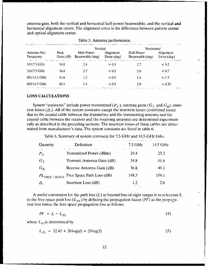
antenna gain, both the vertical and horizontal half-power beamwidths, and the vertical andhorizontal alignment errors. The alignment error is the difference between pattern centerand optical alignment center.
Table 5. Antenna performance.
Vertical HorizontalAntenna No./ Peak Half-Power Alignment Half-Power AlignmentFrequency Gain (dB) Beamwidth (deg) Error (deg) Beamwidth (deg) Error (deg)
315/7.5 GHz 34.8 2.4 < 0.5 2.7 < 0.2
316/7.5 GHz 36.8 2.7 < 0.5 2.6 < 0.5
001114.5 GHz 41.6 1.2 < 0.5 1.4 < V 5
002/14.5 GHz 40.1 1.4 < 0.5 2.0 < 0.25
LOSS CALCULATIONS
System "constants" include power transmitted (PT)' antenna gains (GT and G.), inser-tion losses (IL). All of the system constants except the insertion losses (combined lossesdue to the coaxial cable between the transmitter and the transmitting antenna and thecoaxial cable between the receiver and the receiving antenna) are determined experimen-tally as described in the preceding sections. The insertion losses of these cables are detef-mined from manufacturer's data. The system constants arc listed in table 6.
Table 6. Summary of system constants for 7.5-Gliz and 14.5-GHz links.
Quantity Definition 7.5 GHz 14.5 GHz
PT Transmitted Power (dBm) 29.4 23.2
Gr Transmit Antenna Gain (dB) 34.8 41.6
GR Receive Antenna Gain (dB) 36.8 40.1
PLFR E-SPACtE Free Space Path Loss (dB) 148.3 154.1
IL Insertion Loss (dB) 1.2 2.0
A useful convention for the path loss (L) at beyond line-of-sight ranges is to reference Lto the free-space path loss (LFs) by defining thc propagation factor (PF) as the propaga-tion loss minus the free space propagation loss as follows:
PF = L - LFFS (4)
where LF is determined by
LFS = 32.45 + 20log(d) + 20log(f) (5)
12

for distance d, in kilometers, and frequencyf in megahertz. For a one-way transmissionsystem, signal power at the receiver is
PR = PT + GT - L - IL + GR (6)
Rewriting and using equation (4) the following is obtained:
PF = PT+GT-PR-IL+GR-LFS (7)
AGC voltage, calibrated to power at the receiver PR (equations [2) and [3]), is continu-ously measuicd during link operation thus completing the information required to computethe propagation factor PF Equations (8) and (9) are obtained for the propagation factorsof 7.5 GHz and 14.5 GHz, respectively, by inserting the quantities of table 4 into equation(6).
PF7.5 = - 48.5 - RSL 7.5-GHz (8)
PF 14.5 = -51. 2 -RSL4.5-GHz (9)
13

RESULTS
Measurements began in late January 1992 and continued until May 1992. Eight mea-surement periods, totaling 89 days of operation and over 15,000 observations, were com-pleted during this time. Table 7 lists the continuous measurement periods.
Table 7. Dates of measurements in 1992.
Start EndDate Time Date Time Days
22 Jan. 1100 24 Jan. 0800 1.827 Jan. 0800 27 Jan. 2359 0.728 Jan. 0700 19 Feb. 2359 22.722 Feb. 0001 26 Feb. 2359 5.029 Feb. 0001 03 Mar 1057 3.411 Mar. 0001 27 Apr. 0800 47.305 May 0700 08 May 1300 2.8
11 May 1726 17 May 0046 5.3
One-way transmission-path data are analyzed by comparing observed propagation fac-tors to expected propagation factors for the observed surface meteorology. The evapora-tion duct M profile is calculated from surface meteorological parameters of wind speed. airtemperature, relative humidity, and sea temperature. All meteorological parameters.except ambient sea-water temperature, are averages of those measured at the transmit andreceive site. Only the receive site is instrumented for measuring sea-water temperature.Expected propagation factors are obtained from ML4YER for a given evaporation ductheight 6 . The refractivity profile, as measured in M-units from the air and sea interface upto the evaporation duct height, is determined by the Jeske (1971) method. A "StandardAtmosphere" refractivity profile is assumed to exist above the evaporation duct height.
Nonstandard atmospheric refractivity profiles may produce signal enhancements thatare tens of dB's above the signal levels experienced when the refractivity profile is that ofthe evaporation duct coupled with a standard profile. Figures 8 and 9 provide height versusM-unit profiles for 86 atmospheric soundings obtained at Montgomen' field. San Diego.-alifornia, in the period beginning 28 January 1992 and ending 25 March 1992. Each of
these soundings is labeled STD, SBD, ELEV, or OTHER to indicate if the Ml-unit profile isrepresentative of a standard atmosphere (STD), if it is associated with a surface-based duct(SBD), if it is an elevated duct (ELEV), or if the profile does not clearly fall into thesecategories, hence (OTHER). These soundings are used to explain the behavior of thereceived signal levels and to classify received signal levels, based on whether the atmo-sphere was standard or nonstandard. Because of the ver' great effect that the verticalrefractivity structure above the evaporation duct height plays upon signal strengths, thetime series displayed, beginning with figure 11. were chosen as they coincide with periodsfor which atmospheric soundings were obtained.
14

Sw Sw40o/ / 4W
300• 300
ST R ST3D SBD ELEV 2 S ST SD STD STO
1�02100"
0 0920128050T 920128 1705? 920129 0500T 9201291 MOT 920212 175?T 9202122530T 92U2130505T 920213 1705
Sw 505
4W 400
300! 300!
OTHER STD OTHER STD S2 STO STT STO
20 0 100
0 0920130 0500T 920130 17MT 920131 050T 920131 1700T 920215 15WT 920215 1 IOT 920215 70?T 920215 20=
4W ,K 405
OTHER STD TST STO STD
20S , 200 SS
105 1001
0 092020' 0500T -7202 1 71'T 920202 00T 920207 0600T 920215 230?T 920216 0200T 90216 05WT 92X216 00W
4w 400i
OTHER STD STO SETD w STD OTHER STD SBD2W 2W
100 10.
0 0920207 1 MO1 920206 050T 920 2 O1705T 92021 0500T 920216 1100T 920216 17W0T 92D217 00T 920217 170T
400 400
3M 300
STD STD STD ELEV STD SBD STD ELEV
150
10| || 1I92059 170cr 920209 2300T 92010 050? 92D21011057T 9202'8 0500? 920219 1705? 92219 0920? 92021917?WT
4W 4W
STD STD STD ST 1) 2 ELEV STD ELEV ELEV
100 1001
0 -01
920210 170D7 9210 2305T 920211 17W? 920212 0505? 9202192300? 920222 OSWI 920221705T 920223 05W?
Figure 8. Montgomery field atmospheric soundings from 8 January 1992 through 23 Febru-ary 1992. Each abscissa division is 25 M-un its.

-0 4w3~Im /'/ ,:' oo O HERii
STO SBO OTHER SB OTHER STD STD STD
100 100
0 09O2223 170T 9"20225 0500T 920225 minT 920226 0WT 920318 050"T 9203B 1705 T 920320 05Y 92032D 17010
sm 50
400 400
iSTD SYD OTHER STD STD STD STO STD200
100 // 100 ,
920228 IO0T 920229 2300T 920301 050T 920301 1700T 920321 05WT 920321 hOT 920322 0005 922 7MIOT
400 : ,t
O R STt) I ST OTHER ST2 D OTrER
092302 0500T 920302 1 lOOT 920M 0500T 920311 0500T 920323 1 OOT 920324 0503T 92M24 170OT 920325 050T
400
SBD ST!O OTHER ELEV STD STD
1100
0 0-920311 1700T 920312 0600T 920312 1700T 9203130MOT 920325 1700T 920326 0500T
sm
ELEV ELEV STO STD
200100
9313 1700"r 93=140503T 920314 170WT 920315 050T
400
STD STO OTHER STUam
100
09=15 IO7T 9=r3160500T 920]316 It7T 920317 050T
Figure 9. Montgomery field atmospheric soundings from 23 February 1992 through 26March 1992. Each abscissa division is 25 M-units.
16
SOUTHERN CALIFORNIA COASTAL CLIMATE
The EDCOM experiment was conducted in the southern California coastal area. In thisarea, the coastline runs northwest/southeast. Data from climatic studies (Patterson, 1987)indicate that the most common wind flows north-northwest in the winter and shifts to west-northwest in the spring. This flow is nearly parallel to the coast. Within a few miles to manyfrom the coast, sea breeze effects override the prevailing surface wind. The normal diurnalcycle is as follows: In the morning, the air is still, or blowing off-shore; around noon, theland mass has heated enough to provide the driving head for the sea breeze; sometimebefore dark, the sea breeze reaches its maximum velocity (typically 6 - 14 knots). Whenthe sea breeze is weak, it abates shortly after dark; when strong, the sea breeze may persistuntil late in the evening. Sometime in the morning, the land breeze begins as the land coolsbelow the temperature of the ocean. As the magnitude of the temperature differentialbetween the land and the ccean is less than that experienced with the afternoon sea breeze,the land breeze is usually weaker than the sea breeze, seldom exceeding 10 knots.
Many other factors come into play. Often in winter there tends to be a high pressurezone over the Rocky Mountains. This high pressure tends to drive the continental air massover the ocean in the southern California coastal area. The result is cool dry air over theocean in the coastal area. This flow is in opposite direction to the sea breeze, so while thesea breeze almost inevitably does develop, it is of reduced magnitude and does not persistlong into the evening. Frequently in the summer, there exists a high pressure zone over thePacific Ocean and a low pressure system centered over the Rocky Mountain region. Thispressure differential contributes to the shift of the prevailing winds from being evenly dis-tributed about the northwestern half of the compass rose to being almost exclusively fromwest to northwest. Longer days and higher inland temperatures let the sea breeze fullydevelop, resulting in higher wind velocities persisting longer into the evening.
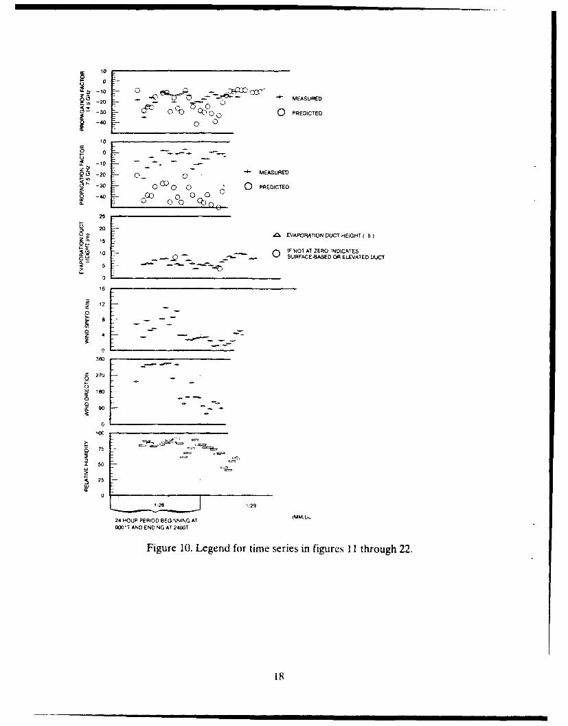
LONG-TERM TIME SERIES
Figure 1) is a legend for the time series presented in figures 11 through 22. The bottomfour plots of figures 11 through 22 include relative humidity, wind direction, wind speedand the resulting evaporation duct height. Air temperature and sea temperature arc alsoused in the computation of the evaporation duct height, but are not shown, as they haveless of a contribution than the wind speed and humidity in the context of the EDCOMexperiment. Surface-based duct height (based upon atmospheric soundings) is shown onthe same plot as the evaporation duct height. Predicted and measured propagation factorsat 7.5 ajid 14.5 GI1z are shown in the top two plots of these figures. The periods of timecovered in figures 11 through 22 comprise approximately half of the measurementsrecorded during the EDCOM experiment. The availability of atmospheric soundings deter-mined the periods chosen.
17
to
10 'SMEASURED
-30 C6 0 0 PREDICTED0 -40f
101
U- 0
z -20- MEASURED_o •, - 0o 0
-30 0 0 0 0 PREDICTEDS-oco oQo000 00 0
25
2041, EVAPORATION DUCT HEIGHT ( b 1O• t5 -
i~x o 0 IF NOT AT ZERO INDICATES21 to SURFACE-BASED OR ELEVATED DUCT4 W
16
CL
3w
z 270
z 9
0
:= 50
25
o -
00
"128 .:29
24 HOUR PERIOD BEGINNING AT (MMUOWIT AND ENDING AT 2400T
Figure 10. Legend for time series in figures 11 through 22.
=. . i I I I I I II 18
10
0
--20 -I "
30 D"0 -40 0 -- -
10
0 0- ---.-. -'- -
z1 0 c- -o -0 -20 C -0 0 " 0 0 0
-00 o, ooo b 0-G-40~ 'J 0
"-40 - O 3 0 0o~~O c° o -ooO< oo
0 L.
20
z 215
25
0 L
1 18
w
1 " _ 2 - 0" 3
360
S270
0
1.)
5 75
100
1 28 ý29 i3
fMM'DO 92)
Figure 11. Time series covering 28 January 1992 through 31 January 1992.
19

C 20 -.--
i ! ! ! ! ' _ _ _-
U-° o -.10 • - -.• , -. "-.--
o 2-0 -- > - ,---- - _,. --' --
-30o -40 - .- - .. , "
zI t
B80
z 27G
9 0
CO
2 -0 -
25
C)1 20 23
20
F -m: I
z 270 I-
rLIo
00
50--
00
2.1 2"2 23 2 4
Figure 12. Time series covering I February 19921 through 4 Februaryi 1992.
20

10
o, -_o o C.,:c' t:r f-Q-Lo -,-.•x:,.,
a- -300 -20 -- - --- -- 2- : ) _-_ -4- - 0"0 -40
-0o o -
O0 -20 <- 0 ' . .- ,.,•,-,.,.
D -30-6)d Ž__,.A--';0 -40 0S,. - - - r-" --- -- .•--,--- ..- ' -• ,, -•
25
0 0
150 ."
0
0~
0 Vr-360
Z 270
0~ 0
75
25
215 210 27 2"8
(MMODD'92)
Figure 13. Time series covering 5 February 1992 through 8 February 1q92.
21

to0
S 0
&- -10 - OD C, T'ýC ca -tý--
"QAN2o -- -- < - ,c-'*°
-20 o ,,•.; JT.
-30 o . -. -. -. -.
-40 -
10
-o 0 0-C-C)
0 -10 7-
0a -2 •C 0C " ',-, ' ,, .
o 0 .... ,=
S 270o 90 - 2' >
25
122
0 20
360
Uj 180 :-.C.- .
Z 90
100
2/9 2:1l0 2'11 2 '2
(MM)OD'92)
Figure 14. Time series covering 9 February 1992 through 12 February 1992.
22

-20 cc)
0- -30
o -40 --
0. 10
o 0
4 -40
25 ,
S 20
z 150
15
10270 -
Sgwo
16
Uj 8
3602
' 270 J
w so
2: 90 -
100
so
125
2;13 2!14 2."S 216
WMMDD92)
Figure 15. Time series covering 13 February 1992 through 16 February 1992.
23
1 0
"-"i 0 0
OU - 20 - ixj , io -30 -. to- C0t o 0 o
1 0
o o40
20
0 -..
0t120 u1_ 0 1.72,020
~~~~~ . . . . l m m m b
-30 000 0~2 y
0 -40 300 0 0 0
20
~; 10 -ý--7-
0
0~12V
0 F
2724
10
10
0 -0 Co " -- C -
1 " -30 ,ooroo ., -
0 -40 c~CL
10
I--., -- -
0 0-10 0 00
0 -ci C 2
16b
30 -2 o '-
o 40
360
IL
25
20
x 180
0 90" =" •••
0
1E
2122/322422
2705
z 90
75-
so --
212 2/20 -1F- -D,92
25 - 25

10C
1 0 t 0.
_,•.-20 '-0- -CS-30
10
-40 _ - --- -
.• 0, o• _..-_ _..::,: --- (.-_ L :•- -.a:
1- 0
U
0 70 -CCC
0• 5
C- 0 -20 C) 0 Q-----
(0 M,"0 D/
25
U!
00
10
126

0 0
'0 -00 - 0 r_ - • -) 0 - - - • -S-o10 - 0"0.., - - C-- - -
0 ,4 --P .. -•-- - --. -. .10 02 G C) C) C-
' -30 - oCD
- -
F- - .. .. o- . 0.; -• • -•
25
10
-1 LU 7
5 0
106
12
Z 270
0 _
-90
30
3]13112 3;13 3'1,4
(MMIDD!192)
Figure 19. Time series covering 11 March 1992 through 14 March 1992.
27
C -m -

S10
-10
° °c- > ._: . t_-- -rcrr•9r. r, 1
~-0 0 0
-20
-30 - -
0 -400- -
lo
-10
00 270 • • •
-10 -
• 25
20
Ca -301. -3ý-
3015 3 !1 3/18
25
0 19 CI
16
160
l27
oC U, 180
0
~ 75
T 5
0,
~ 25
1) 0
-20 0 0 zx9
-20 -4 0
-1 0a. MO-
-20-
-so-_-_ _ _ - -,---0 -, -_- -° - _
0 10 -0
o
-, 0
S-o-10 0 " 0 -,- "
Qa 20
Z t" 15o -300.T0c c0i O 0
10
160
0
360
z 270
180
90
100
50Z 0
S 25
3119 3120 3/21 3/22
(MMIDD/921
Figure 21. Time series covering 19 March 1992 through 22 March 1992.
29
-20 - )-30 4-0 -4 J.-~-'
0 -0 .--
a. o - - - -,- .. .. .
10
I-309c -20 > -'- -
• -° _ C ... -_
10 00-00 OD 0 -.
0
25
20z• 15
0-
r,- 152[
~ 0
360
z 90
00
x 50••
0->9 250
II r3/23 3;24 3/25 3126
(MM/OD/92)
Figure 22. Time series covering 23 March 1992 through 26 March 1992.
30
Figure 11 covers the period beginning at 0800 (local) on 28 January 1992, continuing upthrough midnight on the 31 January 1992. The dominant factor in this time period is thepresence of nonstandard refractivity profiles above the evaporation duct. From figure 8, itis seen that the soundings of 0500 and 1700 on 28 January, and 0500 on 29 January. indi-cate surface-based ducts. Soundings at 0500 on 30 and 31 January, while not qualifying assurface-based ducts (they have slightly positive slopes). are super-refractive profiles. Onlyone of eight atmospheric soundings in this period indicates a standard, or nearly standard,refractivity profile. During this period, propagation faictors seem independent of evapora-tion duct height, with measured values staying between - 10 and +5 dB at 7.5 GI lz, andbetween -30 and -10 dB at 14.5 Gltz. It will be seen later, that when there is a standardrefractivity profile, measured propagation factors are 10 dB (or more) below predicted val-ues at 7.5 GHz, and 20 dB (or more) below predicted values at 14.5 Gltz.
Meteorological trends observed during this period bear examination. The diurnal pat-tern with wind direction is immediately clear. The wind blows from roughly 090 degreestrue from 1800 until 0800 the next morning. Then from 080() until 1800, the wind is blowingfrom the north or the west. On 28 January, the humidity is quite high. which suggests thesource of the air mass is from the ocean. From midday on 29 January until the end of the
period, the humidity is generally less than 60K,, suggesting continental air flow. Windspeeds are moderate. It is not until midday on the 29th that the evaporation duct heightexceeds 10 meters.
A transition in this period of time is from what might be described as Nomial conditions(7V; or greater humidity, conditions dominated by onshore air mass flow) to what will bereferred to as Santa Ana conditions. During Santa Ana conditions, the bulk of the air massflow in the southern California area is offshore: that is, the source of the air mass over thewater near shore is from the continent as opposed to the ocean. This very dry air producesevaporation duct heights ranging from 10 to 20 m. As two of the last three atmosphericsoundings in this period indicated nonstandard profiles, the very high signal levels are notnecessarily attributable to the high evaporation duct heights.
Figure 12 is a 4-day period beginning on 1 February 1992 at 0000 that begins with SantaAna conditions: The wind is directly from the east and the relataive humidity is quite low(351:). The evaporation duct height is correspondingly high, reflecting the large verticaldistance required to go from saturation conditions at the air-to-sea interface to the lowambient humidity of the air mass. During this period, the measured propagation factor at14.5 GI-Iz is around 1(0 dB less than predickcd vaiue, and the measured propagation factorat 7.5 Gltz is 5 to 15 dB above predicted values. Two atmospheric soundings are taken thatday, one at 0500 and the other at 1700 (local time). The first sounding does not indicate asurface-based duct. Howevcr, in the first 50 m, the refractivity profile is less steep than thestandard profile. The sounding at 1700 indicates a 35-m surface-based duct. In the periodbetween both soundings, the predicted and measured propagation factors drop, and the dif-ference between them increases, as a transition is made from Santa Ana to normal condi-tions where any signal enhancement is due to the evaporation duct. The conditions at 1500include an onshore flow and a light wind ranging friom 4 to 8 knots, blowing from the north-west. 1 lumidity is high, greater than 8OW4 , and the evaporation duct height is 8 in, or less.
31

By 1500 on 2 February, the measured propagation factor at 14.5 Gliz is 20 to 25 dB lessthan the predicted value; and at 7.5 GlIz, the measured values are 10 to 15 dB below pre-dicted values.
Late afternoon on 2 February, it appears that the atmospheric structure above the evap-oration duct is nonstandard. By 0100 on 3 February, measured signal levels are 25 dB. ormore, above predicted levels at 14.5 Gltz, and 40 dB above predicted levels at 7.5 Gltz.The wind varies from 350 to 100 degrees true and, as the humidity is dropping, it appearsthere is a continental air flow. From 100( until 1500 on 4 February, the humidity begins torise again, and the wind is from 270 degrees true (seaward), reflecting some sea breezeeffects, but the wind velocity never exceeds 7 knots. The winds shift is out of the south, andthen from the west again, to provide Santa Ana conditions. During this period of time,propagation factors at 7.5 GHz remain very high, but at 14.5 Gltz, they vary over a 40-dBrange. From 2 to 7 February, atmospheric soundings are not available, so it is only sus-pected that nonstandard refractivity profiles are the cause of the high propagation factorsexperienced during this period.
Figure 13, covering the period 5 to 8 February, begins with 40¢C relative humidity andwinds at 8 knots from the east, that is to say, Santa Arna conditions. Propagation factors arein line with those associated with surface based ducts. By 6 February, though it appears thata transition has been made to evaporative ducting conditions, those conditions where therefractivity profile is above the evaporation duct, are standard, or nearly so. Three of foursoundings on 7 and 8 February indicate standard profiles: the other is super-refractive.below 60 meters. These are the conditions that the EDCOM experiment was designed for:conditions where the evaporation duct is the dominant mode of propagation. On 8 and 9February, the signal levels are frequently below detection level. It is only on the 8th of Feb-ruary, when the evaporation duct reaches approximately 8 m, that the propagation factor at14.5 Gltz rises above -40 dB. It should be also noted that on 8 February. the propagationfactor at 14.5 GHz lags the predicted value by a few hours.
The measurement period from 9 to 16 February is shown in figures 14 and 15. All atmo-spheric soundings from the period in figure 8 are standard or nearly so. The humidity is rel-atively high, the wind speeds vary from 4 to 16 knots, and the evaporation duct heights varyaccordingly from 5 to 15 meters. For the duration of this period, measured signal strengthsfollow predicted levels and are about 15 to 35 dB low at 14.5 GHz and 10 to 20 dB low at7.5 Gttz. Note that five soundings were taken each day on 15 and 16 February. All sound-ings, except the very last, indicate standard profiles. These standard profiles consistcntlyincrease the confidence that for this period of time the evaporation duct is the dominantmode of propagation.
Figure 16 covers the period of 17 to 19 February inclusively (the experiment was off-line on the 20th.) Measured propagation factors follow the predicted values as they did infigures 14 and 15. However, atmospheric soundings at 1700 on 17 and 18 February show30- and 45-m surface-based ducts, respectively. It has been observed that surface-basedduct profiles are usually associated with elevated propagation factors. This counter exam-ple illustrates the variability inherent when applying single geographical point measure-ments of the atmospheric refractivity to an entire transmission path. Examining the
32

meteorological parameters, it is seen that the humidity stays generally above 75S/, and thewind is mostly trom the north. Sea breeze effects are seen in the form of increasing windvelocities and more westerly wind direction in the afternoon.
Figure 17 covers the period 22 to 25 February inclusively. From 0001 on 22 Februaryuntil 0800 on 23 February, humidity is 90% or greater, and the evaporation duct heights are
6 m. or less. The first of the two atmospheric refractivity profiles is standard. The secondprofile (1700) indicates an elevated duct that does not appear to have, and should not have,a large effect on signal strengths. Two of the four soundings taken on 23 and 24 Februaryshow nonstandard profiles. The propagation factors are very high. typical of conditionsseen during surface-based ducts or low elevated ducts.
From the soundings and time series discussed so far, the following three generalobservations are made and are borne out by the remainder of the test data:
"* During periods of onshore flow with a standard vertical refractivity profile. prop-agation factors at both 14.5 Gt z and 7.5 GlIz follow predicted values: however,they are typically around 25 dB and 15 dB less than predicted values.respectiveiy.
"* Periods of olfshore flow accompanied by low relative humidity give rise to signallevels that are near predicted values at 14.5 Gttz and exceed predicted values at7.5 GlIz.
"* If some of the soundings in a period of a few days show surface-based or ele-vated ducts, then often, that entire period may have signal levels that are nearpredicted values at 14.5 Gltz and exceed predicted values at 7.5 Gl iz.
Figures 18 through 22 cover those periods between 29 February and 26 March when thesystem was operational and atmospheric soundings were obtained. The figures provide fur-ther examples of the general observations noted. Again, figures 8 and 9 provide associatedsoundings.
CUMULATIVE DISTRIBUTIONS
Distributions of measured propagation factor, and the propagation factor predicted byclimatological and meteorological measurements, are shown in figure 23. The curvelabeled Climatologi, is the distribution of propagation factor predicted by MI4 YER basedupon historical distributions for evaporation duct heights in the southern California area.The curve labeled Predicted is the distribution of propagation factors predicted byMLA! YER based upon meteorological observations at the receive site (predicted distribu-tions based upon transmit site are nearly identical). The curve labeled Measured is the dis-
tribution of actual propagation factor data. At 14.5 Gllz, the 405 point on the ordinant ofthe Measured curve is offset 27 dB from Climnatolo&,g and Predicted curves. Similarly, thepropagation factor corresponding to 10-1) BER is -30 dB, and both Climatology and P're-dicted propagation factors exceed this value 81cl' of time, while the Measured propagationfactor exceeds this value 27% of time.
33

1 Climatology"�"•0Predicted
o 60 -•x 0O
40-
20- E Measured 0
-120 -100 -80 -60 -40 -20 0 2014.5 GHz Propagation Factor (dB)
100
0)0r® 80 1 • • [ Climatologyo 60 Predcted
S 40 -
n
100 -80 -60 -40 -20 0 207.5 GHz Propagation Factor (dB)
Figure 23. Cumulative distributions of climatology predicted. meteorological mea-surement predicted, and measured propagation factors.
At 7.5 GHz, the 5Vý point on the ordinant of the Measured curve is offset 16 dB to theleft of the Climaiolqo&, curve and 12 dB to the left of the Predicted curve. Likewise, thepropagation factor corresponding to 10-6 BER is -30 dB; Climatologv, Predicted, and Mea-sured propagation factors exceed this value 54, 62, and 34cQ of time, respectively.
Cumulative distributions of percent error-free seconds, figure 24, correspond with thoseof the propagation factors. For a time-varying signal, it is expected that when the averagepropagation factor over some moderate time interval is equal to the propagation factorcorresponding to error-free communications ( 10 -) BER). the percentage of time when thesignal is error free will be 5(0%;. As stated before, at 14.5 Gliz, the availability of the signal
34

above the error-free threshold is 27%. From figure 24 it is seen that 26% of the time thepercent error-free seconds exceeds 50%. At 7.5 G6Hz, the availability of the signal abovethe error-free threshold is 34%, and 32% of the time, the percent error-free secondsexceeds 50%.
100
807
O 60
20--
CL 20
00 20 40 60 80 100
14.5 GHz Percent Error Free Seconds
10080-
a)
o 60X
"C 40-a)
20
0 20 40 60 80 1007.5 GHz Percent Error Free Seconds
Figure 24. Cumulative distribution of percent error-free seconds (%EFS).
Consideration of the geographical aspects of EDCOM suggests differentiating betweenOnshore flow as opposed to All Cases that have been discussed so far. Meteorologicalinstruments for EDCOM are located at the transmit and receive site on the shoreline. Withonshore flow (sea breeze), the air mass has traveled over the water and its bulk parameters(air temperature, wind speed, and relative humidity) should be representative of the airmass over the propagation path. During Offshore flow, the air mass has not traveled overthe body of water and its bulk parameters may not be representative of those over the
35

propagation path. Figure 25 shows Measured and Predicted propagation factor distributionsat 14.5 and 7.5 GItz during periods of onshore flow. The difference between the distribu-tions of Measured and Predicted propagation factors during periods of Onshore flow doesnot differ appreciably from the differences between the distributions of Measured and Pre-dicted propagation factor forAll Cases. At 14.5 Gtlz and during Onshore flow, the 36/'point on the ordinant of the Measured curve is offset 29 dB to the leI, of the Predictedcurve. At 7.5 GHz, the Measured curve at the 47% point is offset 15 dB to the left of thePredicted curve. This is a 2 to 3 dB greater difference than seen when considering all cases.
1000) 80
,, 80C) 60Prdcew
C 40S[o Measureda) 20
20
120 -100 -80 -60 -40 -20 0 2014.5 GHz Propagation Factor (dB)
100-
80O 60- PredictedLU)Io 607xW a"-' 40
Measured20
0100 -80 -60 -40 -20 0 207.5 GHz Propagation Factor (dB)
Figure 25. Cumulative distribution for meteorological measurement predicted andmeasured propagation factor for onshore flow.
36

A major goal of EDCOM is evaluating the performance of MLA YER in predicting
propagation factors for a given evaporation duct height. Figure 26 is a scatter plot of
observed propagation factors versus evaporation duct height. MLAYER predicted propaga-
tion factors for a neutral atmosphere are plotted as a solid line. On the 7.5-Gltz plot, there
is a well-defined clustering. The upper cluster (average propagation factor equal to zero) is
most likely due to the effects of surface-based ducts from elevated trapping layers (not
evaporative ducting). At evaporation duct heights greater than 15 m, the distribution does
not appear bi-modal. The 14.5-GHz plot does not show the clustering seen at 7.5 Gi~z
when the evaporation duct height is less than 15 m.
0
o• $ -10 -
,ON -20
.j -3040)
0.o -40-0
o 5 10 15 20
Evaporation Duct Height
202. 10 . _- -- - -
O- - . : , . " ..
-100 c -20 - -"
-50 ": -S " .
L. / . . . , , . , .....
C. -600 5 10 15 20 25
Evaporation Duct Height
Figure 26. Propagation factor versus evaporation duct height for hour averaged propa-
gation factors. The solid lines arc model predictions based upon neutral evaporation
duct profiles.
37

To assess the feasibility of using the evaporation duct as an alternative communicationschannel, it is necessary to separate those observations where the evaporation duct is not thedominant mode of propagation, from those where it is. Figure 27 plots hour averages ofmeasured propagation factors that are within 2 hours of an atmospheric refractivity profilelabeled STD or SBD in figure 8 or 9. The crosses indicate that the measuremcnt isassociated with a standard or nearly standard (STD) refractivity profile, and the trianglesare associated with surface-based ducts (SBD). At 7.5 GHz, roughly half of the measure-ments associated with surface-based duct profiles (triangles) are clustered with propagationfactors ranging from - 10 dB to +5 dB, seemingly independent of the evaporation ductheight. The appearance of the surface-based duct associated measurements at 14.5 Gliz issimilar, except for the upper clustering of propagation factors for the surface-based ductsranging from -20 to - 10 dB. The remainder of the SBD hour averages at both frequenciesare evenly distributed with the STD hour averages.
Measurements where the evaporation duct is the dominant mode (crosses) tend to fol-low the MLAYER prediction curve clearly at 7.5 GHz and less clearly at 14.5 Gliz. It isobserved that almost all of the STD measurements at 7.5 Gliz are in the lower cluster ofmeasurements. Receiver performance, however, must be taken into account when compar-ing propagation factors for a given evaporation duct height for the cases where the evapo-ration duct is the dominant mode of propagation. From figure 7, it is seen that the AGCvoltage no longer varies linearly with received signal level when the propagation factor isless than -50 dB at either frequency. This implies that -50 dB is the lowest measuredpropagation factor that may be used confidently for analysis. When the evaporation ductheight drops below 9 m, at either frequency, many measurements in the lower or evapora-tive ducting cluster are less than -50 dB. There are also very few observations at ductheights greater than 17 m.
Figure 28 is similar to figure 27, except that only STD observations are plotted, and twolinear least squares fit lines have been included on each graph for observations where theevaporation duct height is greater than 9 m and less than 17 m. In both figures, the upperleast squares line is from all evaporative ducting observations. The upper line at 7.5 GHz isapproximately 10 dB less than predicted values. The upper line at 14.5 GHz is approxi-mately 20 dB less than predicted values. It is felt that the upper cluster of measurements inthe 7.5 Gliz plot is due to surface-based ducts that are not reflected by associated atmo-spheric sounding of figures 8 and 9 due to spatial and temporal variations. The lower leastsquares line for both graphs is developed by considering only those observations wherepropagation factor is less than -10 dB at 7.5 GIlz. The line at 7.5 GHz is approximately 7dB less than predicted values, and the line at 14.5 GHz is approximately 23 dB less thanpredicted values. It is felt that when the evaporation duct is the dominant mode of propa-gation, and the evaporation duct height is between 9 and 17 m, the mean value for propa-gation factors will be within a few dB of the lower least squares line and will not exceed theupper least squares line.
38

CO 0
2 -10
-20CLOO04 -30 --"-'---4- -"""
) --4040
-500 5 10 15 20 25
Evaporation Duct Height
2010
"L..30 +/ -,=.-•.
o00"610
LL.c ~ -20
3-300 -40
0)50
05 10 15 20 25Evaporation Duct Height
Figure 27. Propagation factor versus evaporation duct height separating surface andelevated duct observations (triangles) from purely evaporative ducting cases. The solidlines are model predictions based upon neutral evaporation duct profiles.
39

a) 0
0 -10 11 -- -20-
*0 -30°Least Sqaures-40 --
-5,,0 5 10 15 20 25Evaporation Duct Height
CO 20"70-0 10
CO .--10
0 -20'Z- r'- -30CM -40- -...
W -50 Least Squares0
05 10 15 20 25Evaporation Duct Height
Figure 28. Propagation factor versus evaporation duct height from purely evaporativeducting cases with linear least squares fit lines for evaporation duct heights between 9and 17 meters. Unmarked solid lines on each graph are model predictions based uponneutral evaporation duct profiles.
The differences between predicted and measured signal strength are primarily due tohorizontal inhomogeneity. Those periods, where the evaporation duct is the dominantmode of propagation and the winds are light, have the lowest evaporation duct heights.Light winds are normally associated with considerable variability of both wind speed andwind direction. As a result, there are considerable differences in wind speed and direction,and therefore a difference in the evaporation duct height along the path. The nonunifor-mity of the duct may increase the leakage from it, and it may, consequently, reduce the
40

receive site signal levels. At higher wind speeds, both wind speed and direction are nor-mally more uniform. This implies less variability along the path, and a more uniform ductthat minimizes leakage. This may explain the much closer match between prediction andmeasurement at higher evaporation duct heights.
HIGH SPEED TESTS
For a normal (line-of-sight) microwave communications system, multipath fading(Liingston, 1970) is the term used to describe signal strength variation due to phase differ-ences between reflected/refracted rays. For ducted communications, there may be no sig-nificant direct or nonreflected/refracted rays, but rather there may be many different, com-peting rays. Rapid local variations in the atmospheric structure along the propagation pathbring changes in field strength and phase for any particular mode at the receive site. Thetime-dependent interference of these modes leads to large signal variations. Again, deter-mining the micro-meteorology along the path is not practical, so fading characteristics aredetermined experimentally by high-speed sampling of the propagation factor.
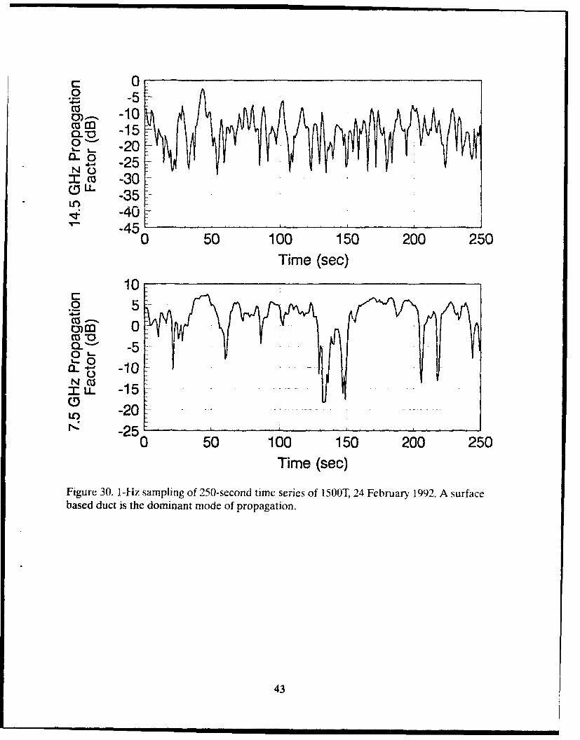
Over 400 time series, having a one-second (1-Hz) sample interval over a 250 secondduration, were taken of propagation factor and bit-error rate during the course ofEDCOM. Figure 29 illustrates propagation factors from one time series taken at 1500T, 9February 1992. From figure 8, it is seen that this is a period when the evaporation duct isthe dominant mode of propagation. For both frequencies, the signal usually stays within 3dB of the median value (propagation factors of approximately -20 dB at 7.5 GHz, and-26 dB at 14.5 GHz). This is fairly typical of the type of time series seen when evaporationducting is dominant. Figure 30 is similar to figure 29, except that it was taken at 1500T on24 February 1992 during surface ducting conditions. The two major differences betweenthese periods are the higher signal levels and greater fading experienced with the surfaceducting conditions. Figure 30 may be considered typical of the conditions seen during sur-face-based ducting conditions.
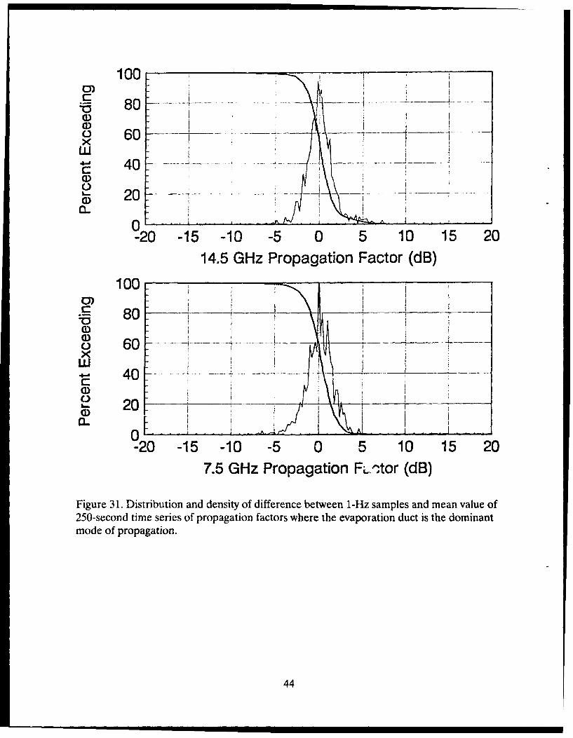
If figures 29 and 30 are truly typical of conditions where the dominant modes of propa-gation are the evaporation ducting and surface-based ducts, respectively, then it is to beexpected that propagation factors during surface-based ducting conditions will be distrib-uted more widely about the mean value for 5-minute samples than those taken duringevaporation ducting conditions. From the discussion of long-term time series and cumula-tive distributions, it is seen that when the evaporation duct is the dominant mode of propa-gation, and when it is less than 15 m, propagation factors at 7.5 GHz are typically less than-10 dB. With very thick ducts, either surface-based ducts or duct heights greater than 15m, the propagation factors typically exceed - 10 dB. Figure 31 plots distribution (thick line)and density (thin line) of one-second samples for all time series when the mean propaga-tion factor at 14.5 GHz is greater than -30 dB, and at 7.5 GHz, mean PF was less than-20 dB, conditions typically associated with those times where the evaporation duct is thedominant mode of propagation. Figure 32 is similar, except it has been developed fromtime series where the propagation factor at 7.5 GHz exceeded -10 dB. Taking numbersfrom the graph, it is seen that, with the evaporation duct, less than 5% of the samples are
41

C -5-0 -107cu ,M0- -15g2.C -200. o-30- _, L- -25
NC.M c -35Lu -40
-450 50 100 150 200 250
Time (sec)
5c.0 0
g•" -54-1COa,-.,-107
0L-MLU -20
LO -25/
"0 50 100 150 200 250
Time (sec)Figure 29. 1-Hz sampling of 250-second time series of 1500T, 9 February 1992. Evaporativeducting is dominant mode of propagation.
42
0,
4 -4 -5::Cz
~ -10a~ -152~ -20.-o •-25* NO
Mct -30--""- U-30)LO .. -3
-1: -40rIT-) -4o-. 00-45 50 100 150 200 250
Time (sec)
10C:0 5
4-A
0-Ct0
CL 4- -10N 0M -- u. -15 _.. ....(D -20r,,: -251
0 50 100 150 200 250Time (sec)
Figure 30. 1-Hz sampling of 250-second time series of 1500T, 24 February 1992. A surfacebased duct is the dominant mode of propagation.
43
100 -
8 0 ..... ... ! . . . . . .CD
Io 60 -~ -K
40 :1
ai)o I
CD 20 -~
0 . . . .-20 -15 -10 -5 0 5 10 15 20
14.5 GHz Propagation Factor (dB)
100
80-a)aICo) 60 - . .- --- -x
40
a)
20
0-20 -15 -10 -5 0 5 10 15 20
7.5 GHz Propagation FL ..tor (dB)
Figure 31. Distribution and density of difference between 1-Hz samples and mean value of250-second time series of propagation factors where the evaporation duct is the dominantmode of propagation.
44

100-CM
80.
o 60oxw
40-
207CL
20 -15 -10 -5 0 5 10 15 2014.5 GHz Propagation Factor (dB)
100-
80-
o 60:
40-C.
020
a. 0 1-20 -15 -10 -5 0 5 10 15 20
7.5 GHz Propagation Factor (dB)Figure 32. Distribution and density of difference between 1-Hz samples and mean value of250-second time series of propagation factors where the evaporation duct is not the domi-nant mode of propagation.
3 dB or more down from the mean signal strength (at zero). Under the conditions wherethe evaporation duct is not the dominant mode, or the duct height is greater than 15 m, 5%of the measurements are 10 dB (or more) down from the mean signal strength.
Bit-error rates closely following the sampled propagation factor suggest that significantaliasing has not occurred in the sampling of the propagation factor. Figures 33 and 34 are250-second time samples of both propagation factor and bit-error rate at 14.5 and 7.5 GHz,respectively; each taken at a period of time when the signal has been near the signal levelwhere the BER is 10-6. On both figures, the bit errors closely follow the sampled propaga-tion factor. It is also seen at the 14.5-GHz time series, in figure 33, that 10-6 BER corre-sponds to a propagation factor of roughly -30 dB; and at 7.5-GHz time series, in figure 34,
45
I i I I I I I II

that 10-6 BER corresponds to a propagation factor of roughly -29 dB. These values agreeclosely with the values plotted in figure 7 for bit-error rate versus propagation factor.
-250
0 -27-CL0
Ic33
o 50 100 150 200 250Time (sec)
-7
-D 6-1-
_j C -4 - _ - - - - - - - -
NL
6L~ -23_ _ __ _ _ _
U) -
o 50 100 150 200 250Time (sec)
Figure 33. One-second interval sampling of propagation factor and bit-error rate of14.5 -GHz signal at 1500T on 3 March 1992.

-2501 -27 -... ...
&2. -290%
N 0 -31
0 -33-351
0 50 100 150 200 250Time (sec)
-7-6 -_
C 0 a -5 4
N b -3
LU -2
0 I0 50 100 150 200 250
Time (sec)
Figure 34. One-second interval sampling of propagation factor and bit-error rate of7,5-GHz signal at 1500T on 17 February 1992.
To provide further information on the time-varying nature of the channel, 4096-pointtime series at 200 Hz-rate were taken of the propagation factor at both frequencies. On 21July 1992, propagation factors at both frequencies were in the linear range of the receiver,and average signal levels indicated the evaporation duct was the dominant mode of propa-gation. Figure 35 shows the first of the described time series taken on that date. At bothfrequencies, it is seen that clearly identifiable minimums occur at intervals ranging from0.5- to 2-seconds. Intervals from deeper minimums occur at larger time intervals. Aver-aged, Parzan (triangular) windowed power spectrum were developed using nine consecu-tive sets of the described 4096-point time series. The results are displayed in figure 36. It isobserved that contribution of frequency components drops rapidly and that the spectrum is
47

essentially flat at frequencies above 10 i{z. This finding agrees with the discussion of bit-error rates and propagation factors in the preceding paragraph.
Co -28
0 -30-
.0 L O
c -34
0
.- -36 0 5 10 15 20
Time (sec)
S-3 3
0 -37 5O
g) -37a-3
0CL_ -41
0 5 10 15 20Time (sec)
Figure 35. 20-1 Iz sample rate time series of propagation factors taken 21 July 1992.
48

1E+006
100000
10000 --
1000
100
10
0.1 5-
0.1 1 10 100
Frequency (Hz)
IE+006
100000
10000 -- -
1000
10010 •---- . . . . . " .
1
0.10.1 1 10 100
Frequency (Hz)
Figure 36. Power spectrum from series of nine, 4096-point, 20-Hz sample rate timeseries of 21 July 1992.
49
100 -- -- ,_ _CIo 80 . -
(D360
u.. 400
20
-40 -30 -20 -10 0Propagation Factor (dB)
U) 100 -- - . _ .C0 80
601
40.0
20
-40 -30 -20 -10 0Propagation Factor (dB)
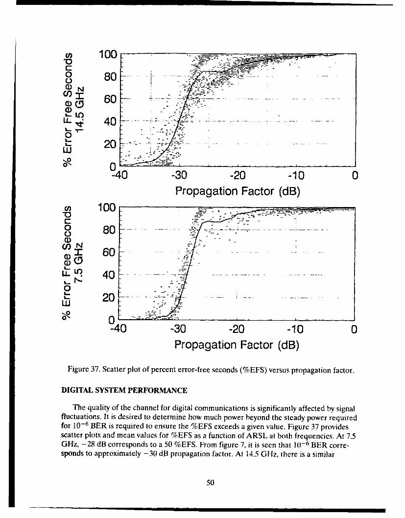
Figure 37. Scatter plot of percent error-free seconds (%EFS) versus propagation factor.
DIGITAL SYSTEM PERFORMANCE
The quality of the channel for digital communications is significantly affected by signalfluctuations. It is desired to determine how much power beyond the steady power requiredfor 10-6 BER is required to ensure the %EFS exceeds a given value. Figure 37 providesscatter plots and mean values for %EFS as a function of ARSL at both frequencies, At 7.5GHz, -28 dB corresponds to a 50 %EFS. From figure 7, it is seen that 10-6 BER corre-sponds to approximately -30 dB propagation factor. At 14.5 GHz, there is a similar
50

correspondence. Using round figures at both frequencies, 4 dB of additional power willprovide 80% error-free seconds; 10 dB extra will provide 90% error-free seconds.
CONCLUSIONS
The evaporation duct strongly influences low-altitude, over water, over-the-horizonpropagation at microwave frequencies. For the geometry and conditions of the EDCOMexperiment, the evaporation duct substantially enhances signal strengths above the diffrac-tion field levels. At 14.5 GHz, the average enhancement is roughly 50 dB; at 7.5 GHz theaverage enhancement is typically 40 dB. At 14.5 GHz the degree of enhancement is typi-cally 20 to 30 dB less than model prediction. At 7.5 GHz the enhancement is typically 15dB less than prediction with the difference between modeled and measured values decreas-ing with increasing evaporation duct height.
Digital signal quality is affected by variations in signal strength. Fading of the signalrequires an increase of power above that level associated with error-free communicationsfor a constant signal level, to achieve a desired percentage of time when the channel iserror free. At both frequencies, 4 dB of additional power will provide 80% error-freeseconds; 10 dB extra will provide 90% error-free seconds. Obviously these figures applyonly to the path and conditions of EDCOM. During conditions where the evaporation ductis the dominant mode of propagation, most fading events are within 5 dB of the 5-minuteaverage signal level. Fading events during surface-based ducting are much deeper thanthose during evaporation ducting, often 20 dB or more. Note, however, that with surface-based ducting, signal levels approach free space at 14.5 GHz and often exceed free spacelevels at 7.5 GHz.
51
REFERENCES
Anderson, K. D. 1991. "Evaporation Duct Communication: Test Plan," NRaD TD 2033(Feb.). Naval Ocean Systems Center, San Diego, California.
Anderson, K. D. 1990. "94-GHz Propagation in the Evaporation Duct," IEEE Trans. Ant.and Prop., vol. 38, no. 5.
Baumgartner, G. B., Jr. 1983. "XWVG: A Waveguide Program for Trilinear TroposphericDucts," NOSC TD 610 (June). Naval Ocean Systems Center, San Diego, California.
Budden, K. G. 1961. The Waveguide Mode Theory of Wave Propagation. Logos, London,England.
Hitney, H.V., J. H. Richter, R. A. Pappert, K. D. Anderson, and G. B. Baumgartner, Jr.1985. "Tropospheric Radio Wave Propagation," Proc. IEEE, vol. 73, no. 2.
Hitney, H. V 1975. "Propagation Modeling in the Evaporation Duct," Naval ElectronicsLab. Cen. Tech. Rep. 1947 (April). Naval Ocean Systems Center, San Diego,California.
Jeske, H. 1971. "The State of Radar-Range Prediction Over Sea," Tropospheric RadioWave Propagation Part 11, AGARD, pp. 50-1, 50-6.
Katzin, M., R.W Bauchman, and W Binnian. 1947. "3- and 9-Centimeter Propagation inLow Ocean Ducts," Proc. IRE, vol. 35, no. 9, pp. 891-905.
Patterson, W L. 1987. "Historic Electromagnetic Propagation Condition DatabaseDescription," NOSC TD 1149 (Sept.) Naval Ocean Systems Center, San Diego,California.
Paulus, R. A. 1985. "Practical Application of an Evaporation Duct Model," Radio Sci., vol.20, pp. 887-896.
Richter, J. H., and H. V. Hitney 1988. "Antenna Heights for the Optimum Utilization of theOceanic Evaporation Duct," NOSC TD 1209 (Jan.). Naval Ocean Systems Center, SanDiego, California.
52

REPORT DOCUMENTATION PAGE OA o.mp 074-18
Public reporting burden for this collection of information is estimated to average 1 hour per response, incduding the time for reviewing istructions, searchig exiting data sources gathering arimaintaining the data needed, and completing and rev¶wMrg the collection of information Send comments regarding this burden estimate of any Other asped of this collection of indoemabon, includingsuggestions for reducing this burden, to Washington Headquarters Services, Directorate for Information Operations and Report. 1215 Jeflerson Davi Highway. Suite 1204 Axi~ngwon VA22202-4302. and to the Office of Management and Budget. Paperwork Reduction Project (0704,O188) Washington, DC 20503
1. AGENCY USE ONLY (Leave blank) 2. REPORT DATE 3 REPORT TYPE AND DATES COVERED
January 1993 Final
4. TITLE AND SUBTITLE 5 FUNDING NUMBERS
EVAPORATION DUCT COMMUNICATION: Measurement Results AC: DN300067
6 AUTHOR.S) PE: 0602232N
L. T. Rogers and K. D. Anderson PN: RC32WI
7 PERFORMING ORGANIZATION NAME(S) AND ADDRESS(ES) 8 PERFORMING ORGANIZATIONREPORT NUMPER
Naval Command, Control and Ocean Surveillance Center (NCCOSC)RDT&E Division TR 1571San Diego, CA 92152-5001
9. SPONSORING/MONITORING AGENCY NAME(S) AND ADDRESS(ES) 10 SPONSORING/MONITORING
AGENCY REPORT NUMBER
Office of Chief of Naval RescarchCode 396600Arlington, VA 22217
11 SUPPLEMENTARY NOTES
12a DISTRIBUTION/AVAILABILITY STATEMENT 12b DISTRIBUTION CODE
Approved for public release; distribution is unlimited.
13. ABSTRACT (Maximum 200 wOrdS)
Results from an experiment to evaluate the performance of an overwater, over-the-horizon, SHF digital communicationsystem are presented. Two simplex microwave digital communication circuits (similar to commercial line-of-sight micro-wave links) are used on an 83-km transmission path that is twice the line-of-sight distance. One circuit is operating at 7.5GHz. The other circuit operates at 14.5 GHz. Both transmitters output a quasi-random bit stream at 1.544-megabits-per-second (DS- 1) that is analyzed at the receiver site.
In a standard atmosphere, the expected received signal level (RSL) is approximately 60 dB below the receiver threshold.However, at these frequencies, propagation modeling shows that, more than half of the time, trapping by the evaporationduct can increase RSL by at least 60 dB.
The propagation path is instrumented at both ends to record surface meteorological conditions and RF characteristics.RSL measurements are compared to predicted levels which are derived from the measured surface meteorology. Industrystandard digital performance measurements are used to assess the effect of RSL variation on link performance. Additionally,results from high-speed sampling of RSL are made to assist in channel characterization.
14 SUBJECT TERMS 15 NUMBER OF PAGES
Super High Frequency Radio 63communications 16 PRICE CODE
S[lF17 SECURITY CLASSIFICATION 18 SECIJRITYCLASSIFICATION 19 SECURITY CLASSIFICATION 20 LIMITATION OF ABSTRACT
OF REPORT OF THIS PAGE OF ABSTRACT
UNCLASSIFIED UNCLASSIFIED UNCLASSIFIED SAME AS REPORT
NSN 7540-01-280-5500 Slanadarr form 298 (FRONTI

UNCLASSIFIED
21 & NAME OF~ RESPONSISIE INOMOUAJ. 21b. TE7fCE~p4 P-**- Code 21C. OFF" SYMW.
L. T. Rogers and K. D. Anderson (619) 553-1413 Code 54W
IS
NSN 7U4O01-ZUo-6600o d pom
UNCLASSIFIED
INITIAL DISTRIBUTION
Code 0012 Patent Counsel (1)Code 02712 Archive/Stock (6)Code 0274B Library (2)Code 50 H. 0. Porter (1)Code 54 J. H. Richter (3)Code543 R.A. Pautus (1)Code 543 L. T. Rogers (25)Code 804 J. W. Rockway (1)Code 804 R.D. Peterson (1)Code 824 J. Rahilly (1)
Defense Technical Information CenterAlexandria, VA 22304-6145 (4)
NCCOSC Washington Liaison OfficeWashington, DC 20363-5100
Navy Acquisition, Research and DevelopmentInformation Center (NARDIC)
Washington, DC 20360-5000
GIDEP Operations CenterCorona, CA 91718-8000
Johns Hopkins UniversityLaurel, MD 20723-6099