active torque vectoring for all wheel drive fsae …
TRANSCRIPT

ACTIVE TORQUE VECTORING FOR ALL WHEEL DRIVE FSAE ELECTRIC CAR
by
VIKAS TUKARAM PAWAR
Presented to the Faculty of the Graduate School of
The University of Texas at Arlington in Partial Fulfillment
of the Requirements
for the Degree of
MASTER OF SCIENCE IN MECHANICAL ENGINEERING.
THE UNIVERSITY OF TEXAS AT ARLINGTON
August 2016

ii
Copyright © by Vikas Pawar 2016
All Rights Reserved

iii
Acknowledgements
First, I would like to express my special thanks to my supervising professor Dr. Robert L.
Woods who has guided me throughout this project, continuously supported and
encouraged by providing plenty of resources and practical solutions during supervision of
this study.
Second, I would like to give a special thanks to UTA racing team and teammates for
constantly believing in me and giving me responsibility to work on this interesting project
associated with their first electric car. After spending over one and half year on team, I
have made bunch of friends in team while doing this project. I am going to remember the
fun stuff we did while finishing this project.
I would like to state my appreciation to my friend Audrey Porter for her patient support and
technical arguments on concept of this project that lead to successful development of this
project. In addition, I would like to appreciate Randy Long for his useful advice and
company. My constant appreciation goes to David Campbell for showing faith and handing
over the responsibility of this project at start of my career on team.
My endless thankfulness goes to my friends Pooja Nale, Ketan Namjoshi and Abhay Bhat
for their encouragement and patient support for joining formula student again. I would have
never join formula student again without their support.
Last not but least thanks goes to my beloved family and friends. They continuously
encouraged, supported and guided me in all stages of my life. I cannot imagine my life
without them.
April 25, 2016

iv
Abstract
ACTIVE TORQUE VECTORING FOR ALL-WHEEL DRIVE FSAE CAR
Vikas Tukaram Pawar, MS
The University of Texas at Arlington, 2016
Supervising Professor: Robert L. Woods
UTA Racing is known for building well-engineered FSAE racecars. This year team
is building, its first electric car by using AWD in-wheel motor concept car E-16. All wheel
drive electric vehicles has an ability to apply instantaneous torque to all four wheels permit
increased car performance.
An ‘Active Model Based Torque Vectoring System controller’ is designed to realize
this objective. The controller was designed to replicate three electronically controlled LSD's
on an all-wheel drive platform with different control strategies. This was achieved based on
the principal of distributing total driver requested torque between wheels, equivalent to the
percentage of the normal load on the tires. Steady state vehicle dynamics models are
combined with on board sensors and driver inputs to calculate normal loads on each wheel.
This system dictates torque to each motor controller in terms of duty cycle based on
measured inputs
v
Torque vectoring system has designed based on two strategies called 3 differential
strategy and 2 differential strategy has implemented in this study. The detailed discussion
about reason behind these strategies are discussed in this study.
MATLAB Simulink program used for programming the torque vectoring controllers due to
ease of programming, debugging, analysis, simulations and automatic conversion to C-
code. .This state based controller has tested using MATLAB program to realize output of
controller program during different driving scenario.

vi
Table of Contents
Acknowledgements .............................................................................................................iii
Abstract .............................................................................................................................. iv
List of Illustrations .............................................................................................................. xi
List of Tables .................................................................................................................... xvii
Chapter 1 Introduction....................................................................................................... 18
Torque Vectoring Concept and Possible Design Philosophies .................................... 18
History and Classification of Torque Vectoring System: .............................................. 20
Classification: Based on Mechanism ........................................................................ 20
Classification: Based on Control Logic ..................................................................... 21
All-Wheel Drive Torque Vectoring ............................................................................ 22
Torque Vectoring System Elements ............................................................................. 22
Sensor Functional Description ................................................................................. 25
Throttle Position Sensor ....................................................................................... 25
Brake Position Sensor ......................................................................................... 25
Hall Effect Sensors............................................................................................... 25
Inertial Measurement Unit (IMU) .......................................................................... 26
Steering Angle Sensor (SAS) .............................................................................. 26
Motor Controller ................................................................................................... 26
Controller Software .............................................................................................. 26
Electronic Control Unit ......................................................................................... 27
Overview ....................................................................................................................... 29
Chapter 2 Motor Modelling ................................................................................................ 30
Introduction ................................................................................................................... 30
Introduction To Brushless DC Motors. .......................................................................... 33

vii
Procedure to Obtain Torque Speed Characteristics: .................................................... 36
Procedure To Obtain Throttle Characteristics For Front Motors. ........................ 37
Step 1: Simulating Characteristics Of Front Motors As Per
Manufacturer Data Sheet. .................................................................................... 37
Step 2: Linear Approximation Of Variable Torque Zone ...................................... 37
Step 3- Find The T And S Axis Intercept For Variable Torque Zone
Line- PeakT And PeakS ............................................................................................ 39
. ............................................................................................................................ 39
Step 4: Finding Characteristic Of Motor For Different Throttle
Position ................................................................................................................ 40
Procedure To Obtain Throttle Characteristics For Rear Motors............................... 42
Step1: Simulating T-S Characteristics Of Rear Motors As Per
Manufacturer Data Sheet. .................................................................................... 42
Step2 : Linear Approximation Of Variable Torque Zone ...................................... 42
Step 3: Find The T And S Axis Intercept For Variable Torque Zone
Line- PeakrT and PeakrS . .......................................................................................... 44
Step 4: Finding Characteristic Of Motor For Different Throttle
Position ................................................................................................................ 45
Procedure to obtain Regenerative Torque Speed Characteristics For
Motors. .......................................................................................................................... 46
Procedure To Obtain Regenerative Characteristics For Front Motors ................ 47
Procedure To Obtain Regenerative Characteristics For Rear Motors ................. 48
Chapter 3 Vehicle Dynamics Model .................................................................................. 49
Introduction ................................................................................................................... 49
Introduction to load transfer .......................................................................................... 50

viii
Longitudinal load transfer calculations ......................................................................... 53
Lateral load transfer calculations .................................................................................. 56
Total lateral load transfer .......................................................................................... 56
Lateral load transfer considering chassis roll ........................................................... 58
Concept of Roll Stiffness .......................................................................................... 58
Simplified Lateral Vehicle Dynamics Model ............................................................. 63
Lateral Load Transfer Considering Unsprung Mass ................................................ 68
Moment due to body roll. .......................................................................................... 69
Moment due to sprung mass roll (At Single axle) .................................................... 70
Moment due to Lateral force acting through roll center. ........................................... 71
Lateral load transfer equation considering unsprung mass ..................................... 71
Combined load Transfer calculation: ........................................................................ 74
Drawbacks of steady state wheel load calculation ....................................................... 77
Need of transient modelling .......................................................................................... 78
Calculation of lateral acceleration based on steering input .......................................... 79
Chapter 4 Torque Vectoring Controller Design ................................................................. 82
Introduction ................................................................................................................... 82
Torque Vectoring Controller Design Philosophies : ...................................................... 83
General layout for Torque Vectoring Controller Program ............................................. 86
Torque Vectoring Controller Algorithm: ........................................................................ 88
Static parameter of Car: ........................................................................................... 90
Input Modifications .................................................................................................... 91
Calculation of Normal load on each wheel .......................................................... 92
Calculation of Total driver requested torque: ........................................................... 93
Calculation of Vectored Torque ................................................................................ 94

ix
Mode -1 – 3 Differential philosophy ..................................................................... 97
Mode-2- 2 Differential philosophy ........................................................................ 97
Modification of Vectored torque on Torque Limit of Motor ....................................... 98
Calculation of Throttle or Regen Position ............................................................... 101
Torque Vectoring Controller Program :....................................................................... 103
Chapter 5 Torque Vectoring Controller Testing and Conversion .................................... 104
Introduction: ................................................................................................................ 104
Range of Input parameters : ....................................................................................... 105
Range of parameter: ................................................................................................... 106
Steering Angle: ....................................................................................................... 106
Throttle Position and Regen brake Position: - ........................................................ 106
Motor RPM ............................................................................................................. 107
Test Matrix .................................................................................................................. 108
Level Testing Output................................................................................................... 111
Level 1 Testing ....................................................................................................... 111
Level 2 Testing: ...................................................................................................... 125
Level_ 2_1 Testing ............................................................................................. 125
Level 2_2 Testing. .............................................................................................. 139
Level 3 Testing ....................................................................................................... 152
Level 3_3 Testing: .............................................................................................. 153
Level 3_4 ............................................................................................................ 158
Level 3_5 and Level 3_6 ................................................................................... 163
Level 3_5 Testing .............................................................................................. 163
Level 3_6 Testing ............................................................................................... 166
Level_3_7 and Level_3_8 .................................................................................. 169

x
Level 3_7 Testing ............................................................................................... 169
Level 3_8 Testing ............................................................................................... 174
Chapter 6 Conclusion and Future Work .......................................................................... 179
Conclusions ................................................................................................................ 179
Future Work ................................................................................................................ 181
Appendix A Motors Data ................................................................................................. 182
Appendix B Motor Controller Programs .......................................................................... 188
Appendix C Torque Vectoring Controller Program ......................................................... 198
Appendix D Torque Vectoring Testing Program Example ............................................. 220
Appendix E List of Symbols ............................................................................................ 229
References ...................................................................................................................... 234
Biographical Information ................................................................................................. 236

xi
List of Illustrations
Figure 1-1 Torque Vectoring Classification ....................................................................... 21
Figure 1-2 Torque vectoring system overview .................................................................. 28
Figure 2-1 Brushless DC Motor Torque Speed Characteristics........................................ 33
Figure 2-2 General Torque Speed Characteristic of Motor ............................................... 34
Figure 2-3 Front Motor 100%: Characteristic .................................................................... 37
Figure 2-4 Linearization of T-S characteristics Data at full duty cycle .............................. 39
Figure 2-5 Front Motors: Throttle Characteristics ............................................................. 41
Figure 2-6 Rear Motors 100% Throttle Characteristics .................................................... 42
Figure 2-7 Linearization of graph rear motors................................................................... 43
Figure 2-8 Rear motors: throttle characteristics ................................................................ 46
Figure 2-9 Front motors regenerative characteristics ....................................................... 47
Figure 2-10 Rear motor regenerative characteristics ....................................................... 48
Figure 3-1 Car from rear view ........................................................................................... 56
Figure 3-2 CG position during chassis roll ........................................................................ 61
Figure 3-3 Car in a turn-Single Axle .................................................................................. 64
Figure 3-4 CG position during roll ..................................................................................... 68
Figure 3-5 Lateral Load Transfer Geometry ..................................................................... 72
Figure 3-6 Procedure for calculating normal load on each wheel .................................... 74
Figure 3-7 Ackerman geometry ........................................................................................ 79
Figure 4-1 .......................................................................................................................... 87
Figure 4-2 Torque vectoring controller program flowchart ................................................ 88
Figure 4-3 Static Parameter .............................................................................................. 90
Figure 4-4 Needs to updated ............................................................................................ 95
Figure 4-5 Needs to be updated ....................................................................................... 96

xii
Figure 5-1 Level_1_1_Mode 1_FL _Throttle................................................................... 113
Figure 5-2 Level_1_1_mode 1_FR _throttle ................................................................... 113
Figure 5-3 Level_1_1_mode 1_RL _throttle ................................................................... 114
Figure 5-4 Level _1_1_mode1_RR_throttle .................................................................... 114
Figure 5-5 Level _1_1_mode1_FL_regen....................................................................... 115
Figure 5-6 Level _1_1_mode1_FR_regen ...................................................................... 115
Figure 5-7 Level _1_1_mode1_RL_Regen ..................................................................... 116
Figure 5-8 Level _1_1_mode1_RR_Regen .................................................................... 116
Figure 5-9 Level _1_1_mode1_FL_Torque Response ................................................... 117
Figure 5-10 Level _1_1_mode1_FR_Torque Response ................................................ 117
Figure 5-11 Level _1_1_mode1_RL_Torque Response ................................................. 118
Figure 5-12 Level _1_1_mode1_RR_Torque Response ................................................ 118
Figure 5-13 Level_1_1_Mode 2_FL _Throttle Response ............................................... 119
Figure 5-14 Level_1_1_Mode 2_FL _Throttle Response ............................................... 119
Figure 5-15 Level_1_1_Mode 2_RL _Throttle Response ............................................... 120
Figure 5-16 Level_1_1_Mode 2_RR _Throttle Response .............................................. 120
Figure 5-17 Level_1_1_Mode 2_FL _Regen .................................................................. 121
Figure 5-18 Level_1_1_Mode 2_FR _Regen ................................................................. 121
Figure 5-19 Level_1_1_Mode 2_RL_Regen ................................................................... 122
Figure 5-20 Level_1_1_Mode 2_RR_Regen .................................................................. 122
Figure 5-21 Level _1_1_mode2_FL_Torque Response ................................................. 123
Figure 5-22 Level _1_1_mode2_FR_Torque Response ................................................ 123
Figure 5-23 Level _1_1_mode2_RL_Torque Response ................................................. 124
Figure 5-24 Level _1_1_mode2_RL_Torque Response ................................................. 124
Figure 5-25 Level_2_1_Mode1_FL_Throttle Response ................................................. 127

xiii
Figure 5-26 Level_2_1_Mode1_FR_Throttle Response ................................................. 127
Figure 5-27 Level_2_1_Mode1_RL_Throttle Response ................................................. 128
Figure 5-28 Level_2_1_Mode1_RR_Throttle Response ................................................ 128
Figure 5-29 Level_2_1_Mode1_FL_Regen Response ................................................... 129
Figure 5-30 Level_2_1_Mode1_FR_Regen Response .................................................. 129
Figure 5-31 Level_2_1_Mode1_RL_Regen Response .................................................. 130
Figure 5-32 Level_2_1_Mode1_RR_Regen Response .................................................. 130
Figure 5-33 Level_2_1_Mode1_FL-Torque Response ................................................... 131
Figure 5-34 Level_2_1_Mode1_FR-Torque Response .................................................. 131
Figure 5-35 Level_2_1_Mode1_RL-Torque Response .................................................. 132
Figure 5-36 Level_2_1_Mode1_RR-Torque Response .................................................. 132
Figure 5-37 Level_2_1_Mode2_FL-Throttle Response .................................................. 133
Figure 5-38 Level_2_1_Mode2_FR-Throttle Response ................................................. 133
Figure 5-39 Level_2_1_Mode2_RL-Throttle Response .................................................. 134
Figure 5-40 Level_2_1_Mode2_RR-Throttle Response ................................................. 134
Figure 5-41 Level_2_1_Mode2_FL-Regen Response .................................................... 135
Figure 5-42 Level_2_1_Mode2_FR-Regen Response ................................................... 135
Figure 5-43 Level_2_1_Mode2_RL-Regen Response ................................................... 136
Figure 5-44 Level_2_1_Mode2_RR-Regen Response ................................................... 136
Figure 5-45 Level_2_1_Mode2_FL-Torque Response ................................................... 137
Figure 5-46 Level_2_1_Mode2_FR-Torque Response .................................................. 137
Figure 5-47 Level_2_1_Mode2_RL-Torque Response ............................................... 138
Figure 5-48 Level_2_1_Mode2_RR-Torque Response .............................................. 138
Figure 5-49 Level_2_2_Mode1_FL-Throttle Response .................................................. 140
Figure 5-50 Level_2_2_Mode1_FR-Throttle Response .............................................. 140
xiv
Figure 5-51 Level_2_2_Mode1_RL-Throttle Response .............................................. 141
Figure 5-52 Level_2_2_Mode1_RR-Throttle Response ............................................. 141
Figure 5-53 Level_2_2_Mode1_FL-Regen Response ................................................ 142
Figure 5-54 Level_2_2_Mode1_FR-Regen Response ............................................... 142
Figure 5-55 Level_2_2_Mode1_RL-Regen Response ................................................ 143
Figure 5-56 Level_2_2_Mode1_RR-Regen Response ............................................... 143
Figure 5-57 Level_2_2_Mode1_FL-Torque Response ................................................... 144
Figure 5-58 Level_2_2_Mode1_FR-Torque Response ............................................... 144
Figure 5-59 Level_2_2_Mode1_RL-Torque Response ............................................... 145
Figure 5-60 Level_2_2_Mode1_RR-Torque Response .............................................. 145
Figure 5-61 Level_2_2_Mode2_FL-Throttle Response .............................................. 146
Figure 5-62 Level_2_2_Mode2_FL-Throttle Response .............................................. 146
Figure 5-63 Level_2_2_Mode2_RL-Throttle Response .............................................. 147
Figure 5-64 Level_2_2_Mode2_RR-Throttle Response ............................................. 147
Figure 5-65 Level_2_2_Mode2_FL-Regen Response ................................................ 148
Figure 5-66 Level_2_2_Mode2_FR-Regen Response ............................................... 148
Figure 5-67 Level_2_2_Mode2_RL-Regen Response ................................................ 149
Figure 5-68 Level_2_2_Mode2_RR-Regen Response ............................................... 149
Figure 5-69 Level_2_2_Mode2_FL-Torque Response ............................................... 150
Figure 5-70 Level_2_2_Mode2_FR-Torque Response ............................................... 150
Figure 5-71 Level_2_2_Mode2_RLTorque Response ................................................ 151
Figure 5-72 Level_2_2_Mode2_RRTorque Response ............................................... 151
Figure 5-73 Level_3_3_Mode1_FL_Torque Response .............................................. 154
Figure 5-74 Level_3_3_Mode1_FR_Torque Response .............................................. 154
Figure 5-75 Level_3_3_Mode1_RL_Torque Response .............................................. 155

xv
Figure 5-76 Level_3_3_Mode1_RR_Torque Response ............................................. 155
Figure 5-77 Level_3_3_Mode2_FL_Torque Response .............................................. 156
Figure 5-78 Level_3_3_Mode2_FR_Torque Response .............................................. 156
Figure 5-79 Level_3_3_Mode2_RL_Torque Response .............................................. 157
Figure 5-80 Level_3_3_Mode2_RR_Torque Response ............................................. 157
Figure 5-81 Level_3_4_Mode1_FL_Torque Response .................................................. 159
Figure 5-82 Level_3_4_Mode1_FR_Torque Response ................................................. 159
Figure 5-83 Level_3_4_Mode1_RL_Torque Response .................................................. 160
Figure 5-84 Level_3_4_Mode1_RR_Torque Response ................................................. 160
Figure 5-85 Level_3_4_Mode2_FL_Torque Response .................................................. 161
Figure 5-86 Level_3_4_Mode2_FR_Torque Response ................................................. 161
Figure 5-87 Level_3_4_Mode2_RL_Torque Response .................................................. 162
Figure 5-88 Level_3_4_Mode1_RR_Torque Response ................................................. 162
Figure 5-89 Level_3_5_1_Mode1_FL_Torque Response .............................................. 164
Figure 5-90 Level_3_5_1_Mode1_FR_Torque Response ............................................. 164
Figure 5-91 Level_3_5_1_Mode1_RL_Torque Response .............................................. 165
Figure 5-92 Level_3_5_1_Mode1_RR_Torque Response ............................................. 165
Figure 5-93 Level_3_6_1_Mode1_FL_Torque Response .............................................. 167
Figure 5-94 Level_3_6_1_Mode1_FR_Torque Response ............................................. 167
Figure 5-95 Level_3_6_1_Mode1_RL_Torque Response .............................................. 168
Figure 5-96 Level_3_6_1_Mode1_RR_Torque Response ............................................. 168
Figure 5-97 Level_3_7_Mode1_FL_Torque Response .................................................. 170
Figure 5-98 Level_3_7_Mode1_FR_Torque Response ................................................. 170
Figure 5-99 Level_3_7_Mode1_RL_Torque Response .................................................. 171
Figure 5-100 Level_3_7_Mode1_RR_Torque Response ............................................... 171

xvi
Figure 5-101 Level_3_7_Mode2_FL_Torque Response ................................................ 172
Figure 5-102 Level_3_7_Mode2_FR_Torque Response ............................................... 172
Figure 5-103 Level_3_7_Mode2_RL_Torque Response ................................................ 173
Figure 5-104 Level_3_7_Mode2_RR_Torque Response ............................................... 173
Figure 5-105 Level_3_8_Mode1_FL_Torque Response ................................................ 175
Figure 5-106 Level_3_8_Mode1_FR_Torque Response ............................................... 175
Figure 5-107 Level_3_8_Mode1_RL_Torque Response ................................................ 176
Figure 5-108 Level_3_8_Mode1_RR_Torque Response ............................................... 176
Figure 5-109 Level_3_8_Mode2_FL_Torque Response ................................................ 177
Figure 5-110 Level_3_8_Mode2_FR_Torque Response ............................................... 177
Figure 5-111 Level_3_8_Mode2_RL_Torque Response ................................................ 178
Figure 5-112 Level_3_8_Mode2_RR_Torque Response ............................................... 178
xvii
List of Tables
Table 2-1 Drivetrain & Weight Characteristics .................................................................. 31
Table 2-2 Chassis Characteristics .................................................................................... 31
Table 2-3 Front Motor –Goodness of fit Coefficient .......................................................... 38
Table 2-4 Rear Motor –Goodness of Fit Coefficients ....................................................... 43
Table 5-1 Torque vectoring controller program test matrix ............................................. 109

18
Chapter 1
Introduction
The goal of this thesis study is to design and simulate active torque vectoring
system for all wheel drive FSAE electric car. While designing of torque vectoring system
decision priority has given in following order, maximize the use of all tires; maximize the
traction, linear predictive response and less driver intervention. This has done by using
development of linear mathematical motor model and steady state vehicle dynamics
models has been used to make torque distribution decision
Torque Vectoring Concept and Possible Design Philosophies
Torque vectoring is power distribution technology to produce improve handling and
traction of vehicle. When car goes around the corner the weight get transferred from inside
wheel to outside wheel as a result of lateral load transfer, also for better handling inside
wheel has to go slower than that of outside wheel to travel same distance. As a more load
on outside wheel/ tire. Outside tire can handle relatively more torque (without slipping) than
inside wheel. This phenomenon concludes that to put more power on the ground, outside
wheels has to receive relatively higher power than inside wheel to improve handling and
traction. In straight line acceleration, weight get transferred from front tires to rear tires as
a result as longitudinal load transfer and all wheel of car run at same speed. For above-
mentioned reasons this phenomenon demands more torque and subsequently more power
on rear wheel that of front wheels. On similar basis while deceleration, front wheel requires
more braking power.
In easiest way, power can be defined for rotating wheel as follows,
𝑃𝑜𝑤𝑒𝑟 = 𝑇𝑜𝑟𝑞𝑢𝑒 × 𝑅𝑜𝑡𝑎𝑡𝑖𝑜𝑛𝑎𝑙 𝑠𝑝𝑒𝑒𝑑

19
From above we can conclude that, distribution of power can be done by controlling
torque on each wheel or by controlling speed on each wheel or controlling both torque and
speed at the same time. Speed control or torque controls are most debated topics in
Vehicle Dynamics and control.
Further, from cause effective analysis, applied torque on wheel produces ground
speed, based on ground resistance at tire contact patch. Therefore, it is evident that
controlling torque is like step ahead thinking, while speed control is like controlling after
effect of applied torque. This mechanism can easily illustrated in following manner.
Wheel speed is a function of applied torque and resistance from ground. To do a
speed control it is necessary to predict the rotational speed of each wheel and distributing
torque to achieve that speed for distribution of power.
On the other hand, If Torque control strategy is applied to distribute torque across
wheel; torque can be controlled independent of ground resistance. Torque control
produces predictive vehicle response across different ground conditions at all four wheels.
This is the reason; we have chosen torque control strategy over speed control strategy.
In this study, we are going to discuss torque control, as this strategy completely
align with, primary goals of this thesis study.

20
History and Classification of Torque Vectoring System:
From 1970, automotive companies started offering antilock-braking system (ABS)
to prevent locking and skidding of wheels by use of electronic sensors technology. In last
decade of past century, further development in sensor and ECU technologies, lead to
development of Electronic Stability control (ESC) system to prevent sideslip of vehicle with
help of ABS system along with other sensor on a car. During the same era, automotive
companies started use of ESC technology to enhance handling and traction of vehicle
during cornering with using ABS. This was starting point for introduction of Passive torque
vectoring. It take quite longer to development of active differentials. This development lead
to introduction of active torque vectoring, where the torque is distributed laterally by
generating braking torque on one wheel , while generating same amount of driving torque
on another wheel
Classification: Based on Mechanism
Torque vectoring system is classified into two parts based on mechanism, active
torque vectoring system and passive torque vectoring system. In active system, torque is
distributed laterally, by reducing torque on one wheel and increasing same amount of
torque on another wheel. On other hand, in passive system lateral distribution is done by
classical mechanical differentials, which unequally distributes the torque based on their
design.

21
Figure 1-1 Torque Vectoring Classification
Functionality for active torque vectoring system can be achieved by two ways,
lateral torque distribution or lateral braking control. In lateral torque, distribution is done
through electronically control differentials while in lateral braking control, different brake
forces are applied on each wheel to produce same effect. Lateral braking control required
over design of brake as well as there is significant loss of torque/ power for working of this
philosophy. Some two-wheel drive vehicle uses the hybrid approach, where driven wheel
uses lateral torque distribution philosophy, while non –driven wheels uses lateral braking
control approach for distribution of torque.
Classification: Based on Control Logic
In addition to above, torque-vectoring system can be classified based on control
logic into three ways, model based, error based, and time based. In model-based system,
static/dynamic models are used to estimate state of vehicle and control decision has made.
Further, in error-based system, sensor input measures the particular parameter (e.g. Yaw,
lateral velocity) and same parameter is calculated for ideal scenario, through other sensor
inputs. The control decision regarding torque distribution is calculated based on error

22
between measured parameter and calculated parameter, so as achieve ideal parameter.
In time-based system, certain transfer function has calculated for distribution of torque, and
time varying torque input are applied to achieve certain parameters values.
All-Wheel Drive Torque Vectoring
In all wheel drive vehicle this approach can be further evolved into distributing
power between front and rear axle with the use of electronically controlled central clutch
system. Depending on design preference, constrained and goals, different philosophies
can be used for distribution of torque in all wheel drive vehicle. However, in all-wheel drive
electric vehicle has significant advantage of applying and controlling instantaneous torque
on each wheel. This will allow to distribute power across all wheels without use of any
mechanical components. This unique feature of all wheel drive electric car allowed making
decision at the level of milliseconds and controlling torque at any instance.
Torque vectoring system maintains grip level while maintaining stability of vehicle across
corner.
Torque Vectoring System Elements
The above is true, when there is power is distributed equally all across four wheel.
However, in case of UTA Racing electric car E-16, two front motors are half the size of two
rear motors. This means from total power, 33% of power is present at front wheels and
67% present at rear wheels. This unequal distribution of power leads to completely different
approach for lateral and longitudinal distribution of torque. This different approach involves
distribution of driver requested torque percentwise on each wheel based on percentage
normal load on each wheel. This kind of philosophy has advantages for avoiding

23
longitudinal and lateral grip at each tire, without exceeding traction limits. Further, in this
study we will discuss implementation of this torque distribution philosophy.
Model based active torque vectoring system has selected to implement above
torque vectoring philosophy. Model based system has advantages over error based and
time based system, they are as follows:
It has flexibility of design
Rapid prototyping of controllers architecture is possible for various application
It has predictive response over wide operating range
It is very easy to debug and test model based controllers
It is easy to interface controllers with vehicle dynamics simulation tools (Ex.
CarSim, Carmaker)
In this system controller, driver inputs (Ex. throttle position, brake position, steering
angle etc.), motor RPM, and inertial measurement unit (IMU) data are used to calculate,
driver intentions and state of vehicle. Driver intentions and vehicle state are combine in
mathematical models to calculate required torque on each wheel. This calculated torque is
then converted into throttle position (duty cycle) for each motor controller.
Active torque vectoring system consist of hardware such as sensors; CAN
communication network, and software. For the function of proposed torque vectoring
system in this study, following sensors are required
Throttle Position Sensor
Brake position sensor
Hall effect sensors
Inertial Measurement Unit
Steering angle Sensor

24
Controller Software
Electronic control unit
Motor Controller

25
Sensor Functional Description
Throttle Position Sensor
UTA Racing E-16 uses drive by wire system .This sensor is installed on throttle
pedal (torque requesting pedal) to measure driver requested throttle. This potentiometer
based position sensor converts dictates throttle pedal position in terms of percentage
travel. The information received from this sensor is used to calculate driver requested
torque in combination with the motor hall effect sensors.
Brake Position Sensor
E-16 uses Mechanical + Regenerative braking approach when it comes for
braking. For this purpose, Split pedal approach, where brake pedal regen is mounted over
hydraulic brake pedals to maximize the use of regen braking. In this system, regen pedal
position is measured by installed potentiometer based position sensor. The information
from this sensor is used to calculate driver requested regen torque in combination the
motor hall effect sensors.
Hall Effect Sensors
Hall effect sensors are install on motor assembly, to measure motor rpm.
Information received from these sensors is used to calculate driver requested torque as
well as convert calculated/vectored torque into input throttle position for individual motor
controllers. In addition, these inputs can be used to longitudinal velocity of car, in case of
IMU failure.

26
Inertial Measurement Unit (IMU)
IMU has installed on car behind driver seat. This IMU unit (VN-200) has capability
equivalent to 3-axis accelerometer, 3-axis Gyroscope, 3-axis magnetometer. This unit
capable linear velocity, linear acceleration, angular position, angular rates along 3 axis.
This sensor uses MEMS sensor measurement in combination with GPS measurements
and onboard Kalman filter to output above-mentioned measurements up to 200Hz. For this
study, information on linear acceleration (longitudinal and lateral), linear velocity is used to
estimate vehicle state at 50 Hz. However, other inputs from the sensors will be useful in
dynamic vehicle dynamics models.
Steering Angle Sensor (SAS)
Steering angle sensor is installed on steering column to measure steering wheel
angle input from driver. This is angular potentiometer indicates steering wheel angle in
terms of degree. The information received from this sensor is used to calculate drivers
steering intentions. In addition, it used to determine IMU unit failure and calculate lateral
acceleration in IMU failure mode.
Motor Controller
The motor controller performs a function of translating calculated duty cycle on the
motors with the help pulse width modulation.
Controller Software
The controller software performs function of controlling sensor inputs into duty
cycle/ throttle position outputs for each motors. These outputs are send to motor controller,

27
to realize desired torque on each motor. For ease of coding and debugging, controller
program has developed on MATLAB –Simulink. C- Code generator tool from Simulink is
used to convert this program into embedded C code. This embedded C code has flashed
on ECU/ Supervisor board micro controller for actual functionality.
Electronic Control Unit
Electronic control unit is installed act as processing unit, which is responsible for
receiving, amplifying, filtering, and processing sensor inputs with help of controller
software, to dictates duty cycle for each motor. This unit communicates with sensors, and
motor by using CAN communication. This unit installed on car near IMU unit embedded in
supervisor board, which handles the other interlocks and other safety protocols and give
extra advantage for smooth operation of controller.
The schematic view of Active torque vectoring system is in given figure. Here the
driver torque request input (throttle position or regen brake position) feed into to car (plant)
through torque vectoring controller via motor controller. This torque request input translates
into driver requested torque in controller, with the help of Hall Effect sensor inputs. In
addition, accelerometer and velocity inputs are used to calculate normal load on each
wheel with the help of steady state equations. Now, this calculated normal load on each
wheel and driver requested are used to desire torque (vectored torque) on each wheel.
This desire torque on each wheel is calculates based on following formula.
𝑉𝑒𝑡𝑜𝑟𝑒𝑑 𝑡𝑜𝑟𝑞𝑢𝑒 = 𝐷𝑟𝑖𝑣𝑒𝑟 𝑟𝑒𝑞𝑢𝑒𝑠𝑡𝑒𝑑 𝑡𝑜𝑟𝑞𝑢𝑒 𝑥 𝑁𝑜𝑟𝑚𝑎𝑙 𝑙𝑜𝑎𝑑 𝑜𝑛 𝑤ℎ𝑒𝑒𝑙
𝑇𝑜𝑡𝑎𝑙 𝑤𝑒𝑖𝑔ℎ𝑡 𝑜𝑓 𝑐𝑎𝑟

28
Figure 1-2 Torque vectoring system overview
This philosophy, gives the advantage of considering, all four wheels at the same
time and equivalent to 3 differentials installed in all wheel drive car. This philosophy gives
a flexibility of transferring 0- 100% torque distribution in between front and rear axle, also
distributing 0-100% of driver requested torque between left to right wheels. In addition, this
philosophy guarantee that all wheels will lose traction at the same time. In some instances,
this philosophy does not able to delivered 100% of driver requested torque due to mismatch
between percentage power and weight distribution.
As per tire data studies mentioned in chapter--- shows that, tires has capacity of
carry a torque more than vectored torque in some instances. This can be implemented into

29
system, by applying two differential strategy. In this, strategy torque and front and rear axle
is distributed laterally by applying following formula
𝑉𝑒𝑐𝑡𝑜𝑟𝑒𝑑 𝑡𝑜𝑟𝑞𝑢𝑒 𝑎𝑡 𝑎𝑥𝑙𝑒
= (𝐷𝑟𝑖𝑣𝑒𝑟 𝑟𝑒𝑞𝑢𝑒𝑠𝑡𝑒𝑑 𝑡𝑜𝑟𝑞𝑢𝑒 𝑎𝑡 𝑎𝑥𝑙𝑒) 𝑥 𝑁𝑜𝑟𝑚𝑎𝑙 𝑙𝑜𝑎𝑑 𝑜𝑛 𝑤ℎ𝑒𝑒𝑙
𝑇𝑜𝑡𝑎𝑙 𝑤𝑒𝑖𝑔ℎ𝑡 𝑜𝑛 𝑎𝑥𝑙𝑒
In-depth discussion about controller strategies will be done in following chapters.
Overview
In Chapter 2, Introduction regarding UTA E-16 car powertrain has introduced. This
chapter has explanation regarding linear motor modelling acquired for this study. In
addition, this chapter would explain advantages of linear motor modelling over nonlinear
motor modelling
In Chapter3, Mathematical models for steady state load transfers are introduced
in this chapter. In this chapter, liner two degree of freedom models are discussed. The sign
conventions, forces on tires, are discussed in this chapter. At the end, advantages transient
models over steady state models has been discussed
In Chapter 4-, torque vectoring controller philosophy has introduced. This chapter
contains details description of controller program logic is explained in details
In Chapter 5-, this chapter deals with testing and debugging methods used for
testing of torque vectoring program. This chapter has in depth discussion on selection of
test matrix for testing of controller program. In addition, it contains discussion on converting
MATLAB program to embedded C program through MATLAB code generation tools.
In Chapter 6-discussion, conclusions and possible future work of this study are
given.

30
Chapter 2 Motor Modelling
Introduction
Design philosophy for this vehicle can be illustrated as,” Analysis of Autocross
vehicle performance stipulates a focus upon cornering potential, due to the vehicle
spending 75% of a course in a turn. All wheel drive electric vehicles have a significant
advantage in this regard due to the ability to apply instantaneous torque to all four wheels,
allowing for increased acceleration on turnout. The vehicle dynamics and load transfer
throughout a normal track cause variation in the capacity of each tire based upon its
respective loading and slip angle. Based upon this understanding, UTA Racing's 2016
electric vehicle design objective was to create an implementation of a suspension,
powertrain and torque vectoring system based upon tire performance data. To accomplish
this goal UTA Racing developed its own motor package, inverter, battery packs and gear-
train in conjunction with the design of own embedded hardware and software control
system”
In compliant with above design philosophy, powertrain specification has been
selected incompliant with FSAE rules. The unequal sizes of power source- brushless
electric motors has been selected due to packaging constrained on car. Parker-Hannifin
the GVK142-50 (142mm diameter, 50 mm stator width) was chosen for a rear outboard
motor package and GVK14225 for the front. The front motors have combined power of 25
KW while rear motor has combined power of 50 KW. These motors are high speed (15,000
RPM), high pole count (12) BLDC design, and in comparison with various sizes of motors
with different attributes, the GVK motor was chosen for a combination of packaging and
very high specific power (6.8kW/kg). These motors are controlled through open loop motor
controller/ inverter by pulse width modulation (PWM).In this study only Mechanical

31
characteristic (Torque- Speed characteristics) is used and these mechanical
characteristics are used to deduce control inputs for motor controller. This approach has
taken due to open loop control design of motor controllers. In order to utilize higher speed
of motors, 13:1:1 dual stage gear box has designed to reduce motor speed. This gear
selection limits the max speed of car about 62 mph.
In addition to above, there are some suspension related specifications of car are
described below. These specifications gives the general platform configuration for E-16
and does not give in depth description about each system design. The weight of the driver
(77 kg) is included in the relevant data points.
Table 2-1 Drivetrain & Weight Characteristics
Characteristic Value Unit
Front Power 25 kW
Rear Power 50 kW
Total Power 75 kW
Front Weight 180 kg
Rear Weight 147 kg
Total Weight 327 kg
Front Weight Dist 55 %
Rear Weight Dist 45 %
Front Max Torque 15 Nm
Rear Max Torque 30 Nm
Front Gear Reduction 13:1 -
Rear Gear Reduction 13:1 -
Table 2-2 Chassis Characteristics
Chassis Tubular Space Frame
Suspension Double Wishbone Adjustable
Brakes Regenerative + Hydraulic
Aerodynamics Front &and Rear
Tires Hoosier 20.5 x 7.0-13 –R25B

32
In this study, it is a very crucial to understand the motors torque speed
characteristics. The brushless DC motors are run by applying pulse width modulated
voltage from power source. This application of voltage has done through motor controller
or inverter that converts power source voltage into different PWM signals. The amount of
time PWM signal is on called as a duty cycle. The motor produces different torque speed
characteristics at different duty cycles. These different characteristics of motors can be
find out from motor’s characteristics at 100% duty cycle/ full load. This chapter will discuss
procedure to find out these characteristics. These methods will be used in further chapters
for calculating driver requested torque as well as calculating inputs for motor controller.
E16 is equipped with drive by wire system, where forward duty cycle are applied
through throttle pedal (or torque requesting pedal) and reverse duty cycle is applied
through regen pedal. This car is equipped with split brake pedal design, where regenerative
breaking pedal is mounted over hydraulic brake pedal for maximizing use of regenerative
breaking. Motor will not able to do individual regen braking in some scenario due to
electrical system design.
This thesis study assumes that, motor are going to produce torque speed
characteristics, as per manufacturer’s data sheet. It is necessary to do actual physical
testing for verifications of these characteristics on motor dyno before system is integrated
on the car.

33
Introduction To Brushless DC Motors.
In general, when duty cycle is applied to brushless DC motors then, it will
produce torque speed characteristics as shown in following figure.
Figure 2-1 Brushless DC Motor Torque Speed Characteristics
This characteristic represents the, variation of torque with speed. As discussed
earlier, amount of speed motor produces is depends upon the amount of load on it. Motor
would able to produce maximum torque at zero speed called as a peak torque. At no load
scenario, motor will able to produce speed called as a rated speed. It is possible to achieve
above-mentioned characteristics of motors electrically but for maximum efficiency of motor
operation, torque of motor is limited to rated torque. Speed of motor is limited to rated
speed (~15000 rpm) for weight efficient, size efficient and durable operation of bearings.
This limit on torque and speed is applied by electrical system through motor and motor
controller design.
34
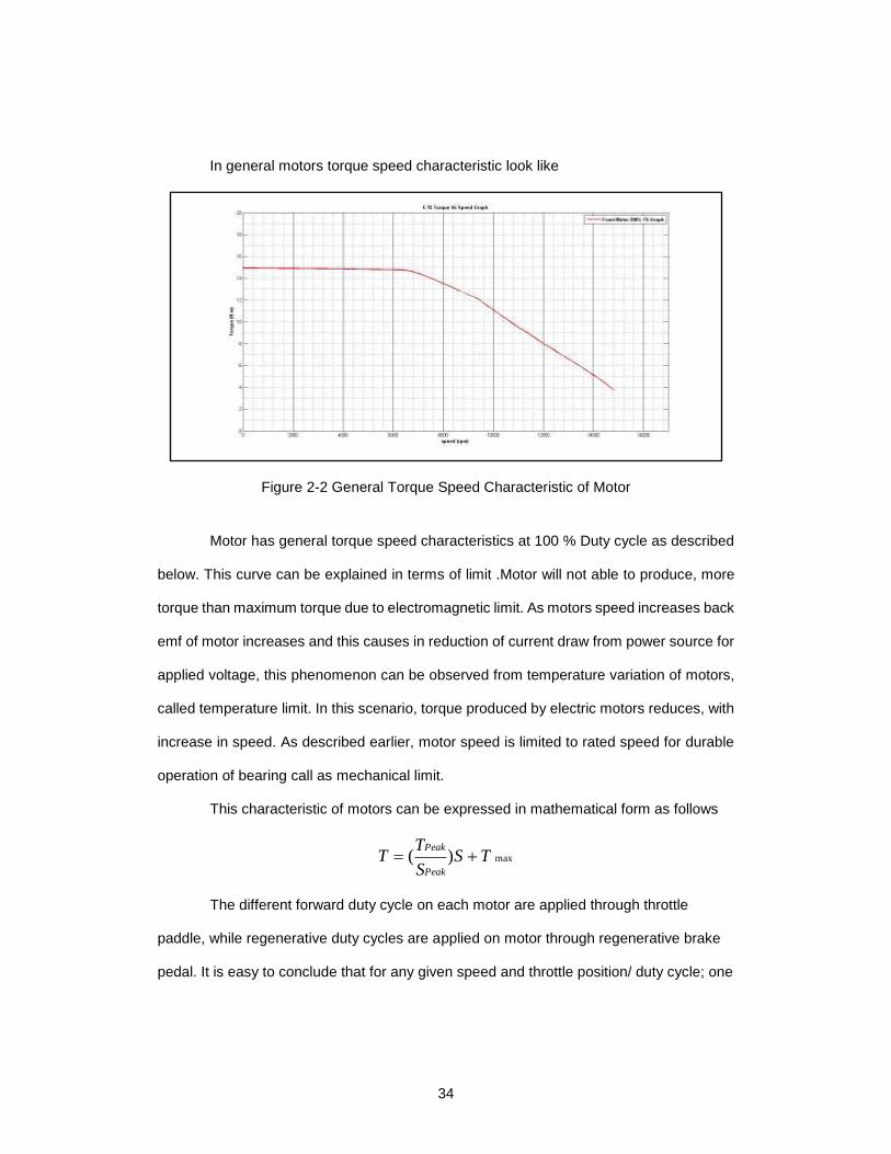
In general motors torque speed characteristic look like
Figure 2-2 General Torque Speed Characteristic of Motor
Motor has general torque speed characteristics at 100 % Duty cycle as described
below. This curve can be explained in terms of limit .Motor will not able to produce, more
torque than maximum torque due to electromagnetic limit. As motors speed increases back
emf of motor increases and this causes in reduction of current draw from power source for
applied voltage, this phenomenon can be observed from temperature variation of motors,
called temperature limit. In this scenario, torque produced by electric motors reduces, with
increase in speed. As described earlier, motor speed is limited to rated speed for durable
operation of bearing call as mechanical limit.
This characteristic of motors can be expressed in mathematical form as follows
max)( TSS
TT
Peak
Peak
The different forward duty cycle on each motor are applied through throttle
paddle, while regenerative duty cycles are applied on motor through regenerative brake
pedal. It is easy to conclude that for any given speed and throttle position/ duty cycle; one

35
can calculate torque produced by motor. The slope of torque speed characteristic is
same as that of the slope at 100 % torque speed characteristic and value of maxT can be
calculated by above-mentioned formula. These characteristic curves for different duty
cycle will look like as follows.
In summary, motor produces different torque speed characteristics for different
voltage duty cycle. In further section, procedure to obtain these torque speed
characteristics will be discussed.

36
Procedure to Obtain Torque Speed Characteristics:
Each motor has two torque speed characteristics, forward duty cycle
characteristics, where power source or battery voltage applied across motors. In reverse
duty cycle characteristics where motor produces back-electromotive force (EMF) and
cause to flow of current from motors to batteries which results into production of
regenerative breaking. In regenerative braking motor acts as generator. Forward
characteristics of both motors are discussed over here in depth and reverse characteristics
results are discussed in this report.
Motors’ manufacturer provide, motor data sheet explaining torque speed
characteristics at 100 % duty cycle as attached in Appendix A. It is possible to obtain torque
speed characteristics for different duty cycle (0 % to 100 %) with linear interpolations. It is
possible to use excel, Mathcad, Mathematica, MATLAB etc. tools to be used for these
interpolations. However to maintain consistency with controller program, MATLAB and
MATLAB curve fit tools is used. This interpolation can be done with following steps.
1) Simulate T-S characteristic of motor at 100% throttle
2) Get the linear approximation for Continuous Torque zone and variable torque zone
3) Find the T and S axis intercept for variable torque zone line- PeakT and PeakS .
4) Obtaining Torque Speed characteristics for different throttle position.

37
Procedure To Obtain Throttle Characteristics For Front Motors.
Step 1: Simulating Characteristics Of Front Motors As Per Manufacturer Data Sheet.
Motor manufacturer provided, torque speed characteristics data at 100 % duty
cycle as attached in Appendix A. This data is used to plot torque speed characteristics of
motor at 100% duty cycle as follows. The program for visualizing this curve
(Front100TScurveGenerator.m) is attached in Appendix B
.
Figure 2-3 Front Motor 100%: Characteristic
Step 2: Linear Approximation Of Variable Torque Zone
Linear approximation of above variable torque- speed zone to find out values of
peak torque PeakT and PeakS or maximum speed. MATLAB curve fitting toolbox used for
linear approximation of torque speed characteristic data. This data has been imported into
matrix format as attached in appendix A and error coefficients generated by different curve
fittings for one-degree polynomial has analyzed for goodness of fit. The following error
coefficient has studied for these tools.

38
The goodness of fit in MATLAB curve fitting toolbox is compared by following
coefficients.
1) SSE (Sum of square due to error)
2) R-Square
3) Degree of freedom adjusted R Square
4) Root Mean Squared Error (RMSE)
Table 2-3 Front Motor –Goodness of fit Coefficient
Robustness of Fit LAR Bi-Square General
SSE 0.3263 0.7085 4.565
R-Square 0.9995 0.9988 0.9924
Adjusted R-Square 0.9994 0.9988 0.9922
RMSE 0.08078 0.119 0.3021
Curve fitting generated by LAR method has selected, after careful study of these
coefficients and generated graphs on curve fitting tools. This curve fit would like as
follows.

39
Figure 2-4 Linearization of T-S characteristics Data at full duty cycle
Step 3- Find The T And S Axis Intercept For Variable Torque Zone Line- PeakT And PeakS .
The MATLAB curve fitting tools provides the equation of line for data points under
considerations. This equation of line can be used to find out, intercept of line on torque and
speed axis. The final equation obtained from curve fitting tools look like:
25.01+0.001415X- =Y
Here, Y represents torque axis while X represents speed axis. The above
equation can be written in terms of torque and speed relation as follows.
25.01+0.001415S- =T
To find out intercept of this line on torque axis can be find out by putting, S=0.
This intercept would give us PeakT .
Therefore,
01.25PeakT Nm

40
Now, to find out intercept of line on speed axis can be found by i.e. PeakS
25.01+0.001415S- =0
Therefore,
0.001415
25.01=SPeak
17674.91 =SPeak Rpm
In summary,
01.25PeakfT Nm
91.17674PeakfS Rpm
Step 4: Finding Characteristic Of Motor For Different Throttle Position
These values of PeakfT and PeakfS would be used for determination of torque
speed characteristics for different duty cycles/ throttle positions. Motor characteristics curve
does not represent negative torque for forward duty cycle because these motors would not
able to do individual regenerative braking due to electrical design of motor controller. If at
any given duty cycle or throttle position motor is speeding faster than that of 𝑆𝑚𝑎𝑥 , it would
produce no torque and it would free-wheeling .
For each duty cycle, the intercept on torque and speed axis is find out by following
equations
𝑇𝑚𝑎𝑥 = 𝑇𝑃 × 𝑇𝑝𝑒𝑎𝑘𝑓
𝑆𝑚𝑎𝑥 = 𝑇𝑃 × 𝑆𝑝𝑒𝑎𝑘𝑓
After obtaining these values, the program iterates values of S from 0 to 𝑆𝑚𝑎𝑥 to
calculate torque at each speed with following equation

41
max)( TSS
TT
Peak
Peak
In addition, another form of above equation can be written as
𝑇 = −𝑇𝑝𝑒𝑎𝑘𝑓
𝑆𝑝𝑒𝑎𝑘𝑓 𝑆 + 𝑇𝑃 𝑇𝑝𝑒𝑎𝑘𝑓
These values of T and S are plotted on graph for each throttle position and
output of program would give following results for forward torque speed characteristic of
front motors. The program for visualizing these curves (FrontTScurveGenerator.m) is
attached in Appendix B.
Figure 2-5 Front Motors: Throttle Characteristics

42
Procedure To Obtain Throttle Characteristics For Rear Motors
The procedure for developing torque speed curves for rear motors is similar to
that of front motors. The motor manufacturer provide data for rear motors as mentioned
in Appendix A. This data represents the torque speed characteristics of rear motors at
100 % duty cycle or throttle position.
Step1: Simulating T-S Characteristics Of Rear Motors As Per Manufacturer Data Sheet.
This data is used to plot torque speed characteristics of motor at 100% duty cycle
and it looks like as follows.
The program for visualizing this curve (Rear100TScurveGenerator.m) is attached
in Appendix B
Figure 2-6 Rear Motors 100% Throttle Characteristics
Step2 : Linear Approximation Of Variable Torque Zone
The MATLAB curve fitting toolbox is used for linear approximation of torque
speed characteristics and error coefficient has studied for different curve fitting for one-

43
degree polynomial by using different robustness method. For linearization of variable
torque zone for rear motors. Data points for rear motors in Appendix A has been
selected for linearization of curve. The points under considerations for front motors has
generated following error coefficient for given robustness of fit options,
Table 2-4 Rear Motor –Goodness of Fit Coefficients
Robustness of Fit LAR Bi-Square General
SSE 9.64 10.18 9.424
R-Square 0.9918 0.9914 0.992
Adjusted R-Square 0.9917 0.9912 0.9919
RMSE 0.4481 0.4604 0.4431
Curve fitting generated by General method has selected, after careful study of these
coefficient and generated graphs on curve fitting tools. This curve fit would like as follows
Figure 2-7 Linearization of graph rear motors

44
Step 3: Find The T And S Axis Intercept For Variable Torque Zone Line- PeakrT and PeakrS .
The MATLAB curve fitting tools provides the equation of line for data points
under considerations and similar to front motors, it would be use to find out intercept on
torque and speed axis. The final equation obtained from curve fitting tools look like
From above curve fit, we have found equation for variable torque region as follows,
44.21+0.002036X- =Y
In other words, we can say that
44.21+0.002036S- =T
Now, put S=0 in above equation to find T intercept of line.
Therefore,
21.44PeakrT Nm
Now, if we put T =0 in above equation to find S intercept of line i.e. PeakS
44.21+0.002036S- =0
Therefore,
0.002036
44.21=SPeak
21714.15=SPeak RPM
In summary, for rear motors
21.44PeakrT Nm
21715PeakrS RPM

45
Step 4: Finding Characteristic Of Motor For Different Throttle Position
These values of PeakrT and PeakrS would be used for determination of torque
speed characteristics for different duty cycles/ throttle positions. MATLAB program----- is
developed for obtaining these characteristics curves. Motor characteristics curve does
not represent negative torque for forward duty cycle because these motors would not
able to do individual regenerative braking due to electrical design of motor controller. If at
any given duty cycle or throttle position motor is speeding faster than that of 𝑆𝑚𝑎𝑥 , it
would produce no torque and it would freewheeling.
Based on motor data, the maximum rated torque of motor has selected as 15 Nm
for front motors.
For each duty cycle the intercept on torque and speed axis is find out by
following equations
𝑇𝑚𝑎𝑥 = 𝑇𝑃 × 𝑇𝑝𝑒𝑎𝑘𝑟
𝑆𝑚𝑎𝑥 = 𝑇𝑃 × 𝑆𝑝𝑒𝑎𝑘𝑟
After obtaining these values, the program iterates values of S from 0 to 𝑆𝑚𝑎𝑥 to
calculate torque at each speed with following equation
max)( TSS
TT
Peakr
Peakr
In addition, another form of above equation can be written as
𝑇 = −𝑇𝑝𝑒𝑎𝑘𝑟
𝑆𝑝𝑒𝑎𝑘𝑟 𝑆 + 𝑇𝑃 𝑇𝑝𝑒𝑎𝑘𝑟
These values of T and S are plotted on graph for each throttle position.
Moreover, output of program would give following results for forward torque speed
characteristic of rear motors.

46
Based on motor data, the maximum rated torque of motor has selected as 30 Nm
for rear motors. The program for visualizing these curves (RearTScurveGenerator.m) is
attached in Appendix B.
Figure 2-8 Rear motors: throttle characteristics
Procedure to obtain Regenerative Torque Speed Characteristics For Motors.
As discussed earlier, the reverse duty cycle is applied on motor through
regenerative brake pedal. Motor acts as a generator, and torque is produced in reverse
direction. The amount of regenerative breaking generated by motor depends on motor’s
rotational speed (or back emf) and state of charge of batteries.
This thesis study assumes that, batteries are at in state of charge, such way that
it is always able to produce maximum regenerative torque/ breaking. In addition, it is
assume that motors produces same torque speed characteristics as that of forward
characteristics. Only difference would be, change in direction of torque produced. These
assumptions allow designing linear motor modelling, without any feedback from motor
controller as well as any electrical feedback. This kind of system is implemented for
simplicity of design.

47
The procedure for development of torque speed characteristics for reverse duty
cycle is similar to that of forward duty cycle characteristics of motors. However
developing negative torque for particular speed and regen brake position.
The equation for calculation of torque is given by.
max)( TSS
TT
Peak
Peak
Procedure To Obtain Regenerative Characteristics For Front Motors
The torque speed characteristics for different regen brake position would look like as
follows.
PeakfT and PeakfS has been calculated earlier. T-S characteristic for different
regenerative position same as that of throttle position. Only difference is that PeakfT has a
negative value. The program for visualizing these curves (FrontTScurveGeneratorRev.m)
is attached in Appendix B.
Figure 2-9 Front motors regenerative characteristics

48
Procedure To Obtain Regenerative Characteristics For Rear Motors
The torque speed characteristics for different regen brake position would look like
as follows
PeakrT and PeakrS has been calculated earlier. T-S characteristic for different
regenerative position same as that of throttle position. Only difference is that PeakrT has a
negative value.
The program for visualizing these curves (RearTScurveGeneratorRev.m) is
attached in Appendix B..
Figure 2-10 Rear motor regenerative characteristics

49
Chapter 3 Vehicle Dynamics Model
Introduction
For simulating torque vectoring controller performance, it is necessary to have real
vehicle or mathematical models of vehicle. The real world track testing helps to understand
controller behaviors and shortcoming from approximation at mathematical models can be
avoided. However, it is not always possible to do real world testing and analysis due to
amount of time needs to spend. So, mathematical models are used to deduce state of car
and control inputs. This helps in making control decisions to enhance performance of car,
almost in any condition.
Based on our torque vectoring philosophy, it is necessary to find out normal loads
on each wheel to make torque application decision on each wheel. Steady state vehicle
dynamics models are used in this study because it is very easy to interpret response of
vehicle in any road conditions. In addition, inputs required for performing mathematical
model readily available with sensors like accelerometer, steering angle sensor, wheel
speed sensor. It is a necessary to know normal loads on each wheel for design of torque
vectoring controller. In this study, steady state vehicle dynamics models are used to
calculate, normal loads on each wheel. These vehicle dynamics model when combined
with sensors data is used for driver intentions as well as torque carrying capacity of each
tire as compare to others. This study uses combinations of longitudinal and lateral load
transfer equations to estimates normal load on each wheel and these estimated loads are
used to make decision on torque application on each wheel.
These models do not consider effects of inertia accelerations yaw, pitch and roll
for simplification. These simplifications of model causes significant certain amount error in
maneuvers like acceleration through corner or breaking through corner. However, these
kinds if maneuver are not racing maneuvers and they does not help in setting fastest lap

50
time on FSAE track condition. These are the reasons, torque vectoring controller is based
on the steady state vehicle dynamics model. If torque vectoring controllers are designed
based on the steady state load transfer equations then it’s possible to extract 90% of car
performance
It is necessary to develop transient vehicle dynamics model with consideration of
inertia acceleration of chassis for increase accuracy of normal load estimation on each tire.
These kind of transient models require higher processing power and mems inertial
measurement units (IMU) because they required feedback from last instant. In these
models, normal load at one instant depends upon state of vehicle at last instant. If adequate
processing power is available and torque vectoring controller design based on transient
vehicle dynamics models would able to extract almost 98% performance of car.
In this chapter, the steady state longitudinal load transfer and lateral load transfer equations
are discussed in detail. Further, the combination of these equations to estimate the normal
load on each wheel are explained. The advantages and disadvantages of steady state load
transfer equations over transient load transfer equations will be discussed . The formulas
to approximate lateral acceleration based on wheel speed sensors and steering wheel
angle have developed. These formulas are used in torque vectoring controller design. This
kind of approach, the controller will able to function in case of accelerometer failures.
Introduction to load transfer
The amount load experience at each wheel statically depends upon the position of
center of gravity. If center of gravity of vehicle is more towards front then front tires
experience more weight than that of rear tires or vice versa. Similarly, if center of gravity is
towards left side of vehicle then load experience by left tires is more than that of right tires.
In E-16 the center of gravity of vehicle is shifted towards little bit at front due to
accumulator container design. The weight distribution between front and rear is 55% and

51
45% respectively at static conditions. Further, it has symmetrical design across vehicle
centerline, so weight distribution between left and right is 50 % each in statically.
When car experiences longitudinal acceleration, inertial load in opposite direction
develops at center of gravity .Now to balance this load , rear tires of the vehicle
experiences more load as compare to static load and this called as load has been
transferred to rear of the car. In case of longitudinal deceleration or braking, this effect
changes direction and front wheel experiences more normal load than static normal loads.
In summary when car goes longitudinal acceleration, load from front wheels is transferred
to rear wheels. However, In case of braking load is transferred from rear wheel to front
wheels. The mathematics involved regarding longitudinal load transfer explained in
longitudinal load transfer section.
The car experiences lateral acceleration, when car goes around the corner. As a
result, car experience centrifugal force and this force is counter reacted by tires producing
equal and opposite forces (centripetal forces). If tires does not able to produce sufficient
reactive force, car goes sideways (or understeers). This lateral acceleration force also acts
at center of gravity and generates the moment. To counter act, this moment outside tires
should experience more normal load than static conditions and it called as load transferred
from inside to outside tires. The amount load is transferring from inside to outside wheel at
front and rear axles is depends upon several factors. There are different formulas are
considered for calculation of longitudinal load transfer. It is very important to understand
physics behind lateral load transfer for understanding to understand load transfer reaction
at front and rear axle. Thomas D. Gillespie explains this physics in-depth in ‘Fundamental
of Vehicle Dynamics’ .However, Gillespie ignores the effect of unsprung mass on lateral
load transfer. Milliken and Milliken considers the effect of unsprung mass on lateral load
transfer into the account in ‘Race car Vehicle Dynamics’ correctly. The different effort to

52
understand this formula has taken into account for understanding of lateral load transfer
formulas. This thesis study broke this formula into different section for understanding of
these effects.

53
Longitudinal load transfer calculations
As described earlier, the normal load experience by each tire on level road
depends upon, position of center of gravity. So, from moment balance around center of
gravity loads on front and rear wheel are calculated by following formula
For front wheels,
l
bWWf
For rear wheels,
l
bWWr
The load on each front wheel can be calculated as 2
fWwhile and
2
rW for each
rear wheel. As explained above when car experiences longitudinal acceleration load gets
transfer from front wheels to rear wheels. The formulas for estimating normal loads on each
wheel can be derived as follows.
Let’s consider a vehicle travelling on level track at longitudinal acceleration the
loads at front and rear wheel are estimated as follows. The longitudinal acceleration xa is
consider as positive and longitudinal deceleration/ braking as a negative.

54
By taking moment around rear tire contact patch + ve - ve
0 cWhDhag
WlW AAxf
In addition, it is interesting to note that,
gaAx lg
Therefore, now we can write above equation for load on front wheel as,
l
hAg
WhDcW
W
xAA
f
Therefore,
l
hWAhDWcW xAA
f
Similarly, by taking moment around front tire contact patch, we can estimates
load on rear wheel as,
l
hWAhDWbW xAA
r

55
In above equation if acceleration is expressed in terms of g’s, then calculated loads
on wheel are mass. However, if acceleration is expressed in terms of standard/ metric
acceleration units, then loads on wheel are force. It is very important to note this because
it may create confusion in units of load transfer.
As car is symmetrical about vehicle centerline. When vehicle is travelling on level
road the above equation for left and right tires can be written as,
For front tires,
l
hWAhDWcWfWW xAA
frfl
22
For rear tires,
l
hWAhDWbWWW xAAr
rrrl
22
From above equations, It can be stated that under vehicle acceleration load on
rear wheel increases and front wheel decreases. Further, In case of deceleration load on
front wheel increases and load on rear wheel decreases.

56
Lateral load transfer calculations
Total lateral load transfer
As discussed earlier, when car goes around a corner, load get transfer from inside wheel
to outside wheels, the amount load transfer at front and rear axle depends upon
suspension and car parameters. However, total load transfer (front and rear combined) is
totally depends upon the CG height. Let look into how to calculate total lateral load transfer.
Assume that car is taking right turn.
Figure 3-1 Car from rear view
Taking the moment equilibrium around point O, we can calculate that,
02
tWtWhWA Ly
t
hWAWW
y
L 2
Also, from weight balance of car

57
WWW RL
Therefore,
t
hWAWW
y
R 2
It is a traditional wisdom to calculate the lateral load transfer forces in terms of
difference or W . It can be defined as amount of normal load added to outside wheel or
the amount of load taken away from inside wheel. This reference is very important for
calculations. This definition is very important to avoid further confusion in lateral load
transfer calculations.
For outside wheel:
WW
WL 2
For inside wheel:
WW
WL 2
Therefore, we can say that:
WWW RL 2
Therefore, the lateral load transfer from inside to outside wheel can be calculated
as follows:
t
hWAW
y

58
This total lateral load transfer almost remains unchanged until; there will be change
in CG height. The above derivation does not considers the chassis roll into account, which
has major impact on lateral load transfer.
Lateral load transfer considering chassis roll
When car goes around a corner, the spring generates displacement. Since springs
are the devices that can generate forces upon displacement, these forces generates
moment that tends to resist rotation of body. This leads to forces on the springs reacted by
tires and it contributes to lateral load transfer. The contribution of lateral load transfer due
to chassis roll has significant contribution to total lateral load transfer, as FSAE cars are
lightweight cars. In addition, when car rolls, the CG of the car deflects side wards and it
gives rise to another moment and contributes to lateral load transfer.
Concept of Roll Stiffness
Before continuing on lateral load transfer, it is important to understand roll stiffness
concept. The contribution spring deflection to generate moment can be quantified as
follows
KM
The roll stiffness at any axle can be interpreted as, when two springs separated by
finite distance, they would act as a torsion springs. Suspension at each axle can be
represented as two spring connected between ground and chassis, separated by distance.
The stiffness of spring acting between depends upon the following
Effective stiffness of spring in between Sprung and unsprung mass or wheel rate
Tire stiffness
ARB Stiffness

59
The effective spring between chassis and wheels (unsprung mass and sprung
mass) called as a wheel rate. In general, this spring attached with wheels via, bell crank
mechanism to reduce the spring deflection to reduce spring deflection to keep it in linear
range and this increases the force on spring. So equivalent stiffness of the spring in
between chassis and wheels can be calculated as follows,
Suspension spring stiffness can be calculated as,
ntDisplaceme
ForceKS
Equivalent, spring stiffness can be calculated as follows,
22 MRKMRntDisplaceme
Force
MR
ntDisplaceme
MRForceK SW
The motion ratio can be calculated from wheel side (less than 1) or can be
calculated from spring side (greater than 1). The motion ratio from wheel side has
considered in above-mentioned equation)
In suspension, the tire and effective suspension spring (wheel rate and tire
stiffness) are considered to be in series, as application of forces on tires produces unequal
displacement in them. The equivalent stiffness between spring and tire can be calculated
by following formula.
TWH KKK
111
Therefore:
TW
TWH
KK
KKK

60
This is the equivalent spring stiffness between tire contact patch and chassis. So
the roll stiffness / torsional spring between two springs can be calculated as follows.
25.0 tKK HW
Now, the above formula represents the equivalent torsional spring between tire’s
contact patch. This spring is attached to ARB and it also adds the roll stiffness depending
on the motion ratio. The ARB torsion spring and above-mentioned torsional spring are
consider to be in parallel. The equivalent roll stiffness at any axle can be calculated as
follows.
ARBwa KKK
These ARB torsion spring are effective when car is in turning scenario, otherwise
they do not affect function of suspension springs. As, chassis is assumed to perfectly rigid
for these equations, so it does not contribute to roll of car. Therefore, total roll stiffness of
suspension of car can be calculated as,
RF KKK
The amount of total lateral load transfer considering roll, can be quantified as,

61
Figure 3-2 CG position during chassis roll
In above figure the sideway moment of center of gravity of car has been considered
for calculation of total lateral load transfer. From above diagram, taking moment around,
roll axis
0sin22
cos syRLsy hWAt
Wt
WhWA
But the roll angle for FSAE car is generally in the range of 1-2 degrees, so
1cos and sin , so above equation can get modified into:
sysyRL hWAhWAt
WW 2
)(
Therefore total load transfer considering roll can be calculated as

62
2
)(t
hWAhAWWW
sysy
RL
Therefore,
t
hWAhWAW
sysy 2
In above equation the sprung mass CG and vehicle CG are assumed to be at same point.
Also the unsprung mass is assumed to negligible as compare to sprung mass ( %10
of total weight). In addition, it is easy to note that,
WWW RL
Therefore,
2
WWL
t
hWAhWA sysy
t
hWAhWAWW
sysy
R
2
If chassis assume to be rigid body then roll moment generated at CG is resisted
by suspension roll stiffness moment. Therefore:
RF KKM
Total suspension stiffness
RF KKK
Hence,

63
KM
In addition, from the moment balance, the moment at CG can be defined as
sysy hWAhWAM
Therefore,
sysy hWAhWAK
s
sy
WhK
hWA
Therefore,
sRF
sy
WhKK
hWA
In summary total lateral load transfer by considering 1-D chassis, roll as follows:
t
hWAhWAW
sysy 2
sRF
sy
WhKK
hWA
Simplified Lateral Vehicle Dynamics Model
Though the total lateral load transfer remains the same, it is important to know the
amount of lateral load transfer is occurring at front and rear axle of car. This amount of load
transfer depends upon the roll stiffness, roll center height, perpendicular distance between
CG and roll center height. The contribution of roll component in FSAE car is significant,
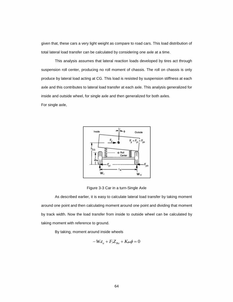
64
given that, these cars a very light weight as compare to road cars. This load distribution of
total lateral load transfer can be calculated by considering one axle at a time.
This analysis assumes that lateral reaction loads developed by tires act through
suspension roll center, producing no roll moment of chassis. The roll on chassis is only
produce by lateral load acting at CG. This load is resisted by suspension stiffness at each
axle and this contributes to lateral load transfer at each axle. This analysis generalized for
inside and outside wheel, for single axle and then generalized for both axles.
For single axle,
Figure 3-3 Car in a turn-Single Axle
As described earlier, it is easy to calculate lateral load transfer by taking moment
around one point and then calculating moment around one point and dividing that moment
by track width. Now the load transfer from inside to outside wheel can be calculated by
taking moment with reference to ground.
By taking, moment around inside wheels
0 aRayao KZFtW

65
t
KZFW
aRayo
By taking moment around outside wheel
0 aRayai KZFtW
Now,
a
aRayi
t
KZFW
As described earlier it’s advisable to calculates load transfers in terms of W ,
As we know from definition of W , described in lateral load transfer due to chassis roll
WWW io 2
Now substituting the values in left hand side of above equation,
Wt
KZF
a
aRaya
22
Therefore,
a
aRay
t
KZFW

66
This is the lateral load transfer at single axle. It can be generalized for front and
rear axle as follows.
For Front axle
F
FRFFy
Ft
KZFW
For rear axle
R
RRRRy
Rt
KZFW
In this section all the assumptions are similar to section lateral load transfer due
to chassis roll. In this section calculations for chassis roll angles remains same and it is
given by,
sRF
sy
WhKK
hWA
The assumption for above equation is ignores the effect of yaw, so the lateral
acceleration experienced by front and rear of car is same. Therefore,
0 cFbF yRyF
And
yyRyF WAFF
cbl
Therefore, solving above equations,
YFyyF AWAl
bWF

67
YRyyF AWAl
bWF
In summary simplified lateral load transfer can be calculated as,
For front
F
FRFFy
Ft
KZFW
For rear,
R
RRRRy
Rt
KZFW
Roll angle is given by,
sRF
sy
WhKK
hWA
YFyF AWF
YRyF AWF

68
Lateral Load Transfer Considering Unsprung Mass
In above derived equations for lateral load transfer it does not considers effect of
unsprung mass. When the unsprung mass is higher than 10% mass of car, it has significant
effect on lateral load transfer. The consideration of unsprung mass changes the few things,
total lateral load transfer is being calculated at each axle, while the total lateral load transfer
remains the same as explained in lateral load transfer due to chassis roll .While considering
this, it is necessary to understand changes in assumption. The car will be treated as a three
mass system consisting of sprung mass, front unsprung mass and rear unsprung mass.
The load transfer is calculated on same philosophy by taking moment around point on the
ground and then dividing it by track width.
In this system, lateral acceleration acts through the sprung mass CG and producing roll
around the roll axis of car, this can be represented as
Figure 3-4 CG position during roll
As chassis is assumed to rigid body, the moment around roll axis can be defined
as,

69
RF KKM
Now the value of roll angle can be calculated by following formula.
sRF
sys
WhKK
hAW
Now this estimated value of roll angle can be used to calculate moments generated
by different masses around each axle. The lateral load transfer can be divided into following
components,
Moment due to body roll
Moment due to sprung mass roll
Moment due to lateral force acting through roll center
Unsprung mass moment
Now these moments can be estimated as follows.
Lateral Laod Transfer =
Moment due to body roll+Moment due to sprung mass roll+moment due to lateral force through roll center+Unsprung mass moment
Track
Moment due to body roll.
As described earlier lateral load transfer force act through the roll center, due to
separation between sprung mass CG and roll axis moment is generated. The distribution
of this moment is proportional to the, roll stiffness of each axle. The calculation for this
moment is as follows,
Moment due to roll = rollM = aK

70
Moment due to roll at any axle can be calculated as follows,
Moment due to body roll
ssRF
sys
arollWhKK
hAWKM
Moment due to sprung mass roll (At Single axle)
It is interesting to note that above-mentioned formula only calculates load transfer
due to sprung mass shift at CG of sprung mass. However, each axle only support the
fraction of sprung mass and it is necessary to take into account the sprung mass shift at
individual axle due to roll. Further, it assumes that distance between sprung mass CG and
roll axis is same at each axle. Therefore, moment due to sprung mass shift at each axle
can be calculated as follows,
sSsasprungroll hWM
Now value of sprung mass at each axle, in case of no longitudinal acceleration
while turning , it can be estimated as follows.
SSsa Wl
xlW
It is interesting to note that, this value, of sprung mass changes depending upon
acceleration or deceleration through corners. For this this thesis study, it assumes that
during combination of lateral and longitudinal acceleration. The longitudinal acceleration
results into change of sprung mass.
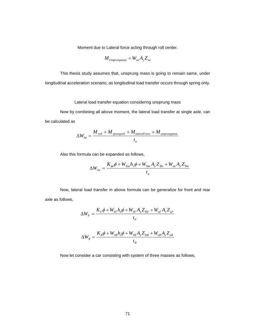
71
Moment due to Lateral force acting through roll center.
uayuassUnsprungma ZAWM
This thesis study assumes that, unsprung mass is going to remain same, under
longitudinal acceleration scenario, as longitudinal load transfer occurs through spring only.
Lateral load transfer equation considering unsprung mass
Now by combining all above moment, the lateral load transfer at single axle, can
be calculated as
a
ssunsprungmacelateralForsprungrollroll
Sat
MMMMW
Also this formula can be expanded as follows,
Now, lateral load transfer in above formula can be generalize for front and rear
axle as follows,
F
uFyuFRFySFsSFF
Ft
ZAWZAWhWKW
R
uRyuRRRySRsSRR
Rt
ZAWZAWhWKW
Now let consider a car consisting with system of three masses as follows,
a
WayuaRaySsasSsaa
Sat
ZAWZAWhWKW

72
Figure 3-5 Lateral Load Transfer Geometry
Now considering, the above diagram and assuming, there is no longitudinal load
transfer. The sprung mass and unsprung mass at each axle can be expressed as follows
Ss
SF Wl
alW
Ss
SR Wl
aW
Now load transfer equations can be represented as follows,
F
uFyuFRFySs
sSs
F
Ft
ZAWZAWl
alhW
l
alK
W
R
uRyuRRRys
sSs
R
Rt
ZAWZAl
ahW
l
aK
W
And the value of, can be calculated as follows,
sRF
sys
WhKK
hAW

73
The above equations can used in case of pure lateral load transfer. In case of
combination of lateral and longitudinal load transfer, it is necessary to estimate value of
sprung mass at each axle based on longitudinal load transfer.

74
Combined load Transfer calculation:
When car goes around a track, Car experiences longitudinal acceleration,
longitudinal deceleration, lateral acceleration, lateral acceleration+ longitudinal
acceleration, lateral acceleration+ longitudinal deceleration. These load cases can be
generalized by calculating loads in following order,
Figure 3-6 Procedure for calculating normal load on each wheel
The longitudinal load transfer can be calculated as,
Load on front tires,
l
hWahDWcW
AAf
lg
Therefore, the front sprung mass can be estimated as
l
hWahDW
l
alW
AA
Ss
SF
lg
Load on rear tires can be calculated as
l
hWahDWbW
AA
r2
lg

75
Therefore, the rear sprung mass can be estimated as follows
l
hWahDW
l
aW
AA
Ss
SR
lg
Now these calculated loads at each wheel can be used to estimate lateral load transfer as
follows,
Lateral load transfer at front axle,
F
uFyuFRFySFsSFF
Ft
ZAWZAWhWKW
Lateral load transfer at rear axle,
R
uRyuRRRySRsSRR
Rt
ZAWZAWhWKW
Now after estimating lateral load transfer, the normal load at each wheel can be calculated
as follows, for right hand turn,
F
f
fl WW
W
2
F
f
fr WW
W
2
R
r
rl WW
W
2
R
rrr W
WW
2

76
E-16 has unsprung mass equivalent to 20% (Approx. due to in- wheel motor
packages) weight of the car. This means, unsprung mass has significant contribution in
lateral load transfer calculation. This is the reason lateral load transfer considering
unsprung mass has used for design of torque vectoring controllers. Sign convention used
in this thesis study are SAE vehicle axis system. The assumption made during calculation
of above equations
CG of the car does not change during dynamic maneuvering- It neglects effect of
fluid movement
The effect of inertial acceleration are not considered – Load transfer due to inertia
neglected
The effect of yaw velocity and yaw accelerations are neglected- Front and rear
axle experiences same lateral acceleration
The chassis assumed to be perfectly rigid body –Same roll angle at front and rear
All the load transfer occurs through springs- Only sprung mass changes during
load transfer 0% anti dive and anti-squat
The location of roll center doesn’t changes in dynamic maneuvering
The principle of linearity and superposition is valid –The series of effects
considered concurrently is identical to sum of individual effects considered
individually.

77
Drawbacks of steady state wheel load calculation
When car goes through series of maneuvers, the fluid like cooling water, brake
fluid etc. moved inside reservoirs, fluid lines and driver moment inside a car. This effects
the position of center of gravity. As driver is strapped firmly with seat belt and the weight of
fluid as compare to weigh of car is less. These effects has minimal impact on car and they
can be neglected for most of maneuvers. However, during certain maneuvers change in
CG can produce significant error in normal load calculations.
The car chassis has certain inertia. Car produces roll, yaw and pitch acceleration during
maneuvering. This acceleration contributes to producing error in calculation of normal load
estimation at each wheel.
When car goes around a turn, car changes direction .This change in direction
produces yaw velocity and yaw acceleration while going around the corner. This difference
in yaw velocity causes difference in lateral acceleration experience by front and rear axle.
The assumption of neglecting yaw acceleration is primary reason of error in lateral load
transfer calculations.
The steady state load transfer equation assumes that, chassis is perfectly rigid
body. However the chassis has own stiffness. This stiffness contributes to flexing of chassis
during turning maneuvers causing difference in roll angle at front and rear axle. This leads
to error in lateral load transfer calculations.
When car experiences longitudinal load transfer, some amount of load goes
through springs and some amount load goes through A-arms. The load going through
spring increases sprung mass and load going through A-arms increases unsprung mass.
This amount of load going through A-arms depends upon side view swing arm angle (SVSA
angle) and longitudinal acceleration. The assumption that all load is going through spring
introduces error in normal load estimation.
78
The maneuvering of car cases moment of suspension component relative to each
other. This moment leads to change in location roll center at front and rear axle depending
on suspension kinematics design. This change in location of roll center leads to error in
calculation of lateral load transfer.
The principle of linearity is valid only if car is goes from one state to another state
smoothly. In case of sudden maneuver (sudden turning, breaking or acceleration) causes
change in normal load of wheel abruptly. This change may not be linear.
Need of transient modelling
It is evident from above drawbacks that the estimation of normal load from steady
state equation can lead to errors in estimation. To estimate the exact state of car at one
moment, it is necessary to know the state of car in previous moment. These errors can be
reduced by doing extensive mathematical modelling with feedback loop or by experimental
testing. The reducing assumption in steady state modelling required effort in mathematical
modeling with advanced sensor technology. These advance sensors will estimate inertial
velocities and inertial accelerations. The mathematical modelling based on advanced
sensor input would help to reduce the error in calculation of normal load transfer.
The amount of development time required to produce these mathematical models
is much higher. This was first year for UTA racing to develop electric racecar and torque
vectoring. The controller design is based upon steady state load transfer equations. As
90% of performance of the car can be achieved with the help of controller based upon
steady state equation.

79
Calculation of lateral acceleration based on steering input
The driver give a steering input and depending on steering angle inside and
outside wheel makes angle depending upon the steering geometry. The steering geometry
for most automobiles are designed to be such that all wheels are pointing towards common
point of rotation. This geometry called as Ackerman geometry.
If the inside wheel angle and outside wheel angles are known, then they can be
used to estimate radius of turn. This radius of turn combine with vehicle velocity, gives a
lateral acceleration. The lateral acceleration based on speed and radius of turn is estimated
by following formula
R
VAY
2
This radius of turn for given vehicle can be calculated as follows,
Figure 3-7 Ackerman geometry

80
The value of riR can be estimated as follows,
i
ri
lR
tan
Now, Value of R can be expressed as,
22)5.0( ctRR Rri
In above scenario, the following assumption has made
The effect of toe angle has been neglected
The effect of tire slip angles on calculation of radius of turn neglected
Steering geometry is symmetrical to left and right
The instantaneous radius of tire is similar to static radius.
The velocity of car can be estimated by converting wheel rpm of from each wheel by using
following formula.
motorTSW GSRV 2
Now by taking average for velocity of all wheels, the average velocity of car can be
expressed as follows.
4
rrlrfrfl VVVVV
The speed difference between inside and outside wheel has considered to negligible, in
above estimation.

81
Though this estimation does not able to produce exact values of lateral
acceleration due to above-mentioned assumptions, it will be helpful for estimation of
approximation of lateral acceleration. This approximation can be proved very useful during
on board accelerometer failure and there by providing torque biasing. These equations are
used to approximate lateral acceleration, when accelerometer failure is detected. The
accelerometer failure is detected by comparing steering angle values and lateral
accelerometer readings. It has explained in next chapter.

82
Chapter 4
Torque Vectoring Controller Design
Introduction
This chapter explains torque vectoring controller working and philosophy. The
main objective of torque vectoring controller is to maximize the use of all tires at any
situation by distributing driver requested torque across all four wheels. Two philosophies
(3- differential or 2- Differential) are used to design this controller due to unequal
distribution of power and weight. To account for accelerometer failure, torque-vectoring
controller based on steering wheel has discussed in this chapter. This chapter discuss
philosophies and algorithm of torque vectoring controller
This controller software runs on E-16’6 supervisor’s board. This supervisor board,
collects data from various sensors and torque vectoring controller program estimates the
state of car, convert this data into duty cycles for motor controller. Motor controller uses
these inputs for application of desired torque as explained in chapter 2. The torque-
vectoring program run on embedded controller chip. This chip requires controller program
in C for its operation.
The MATLAB Simulink program has used for programming of this controllers. As
MATAB Simulink has following advantages over other programming language.
It is easy to do programming due to inbuilt functions
It is easy to debug programs, as program indicates the error and location.
It is easy to convert MATLAB Simulink program to C with inbuilt function
It is easy to interface with various vehicle dynamics software for simulation

83
Torque Vectoring Controller Design Philosophies :
The E- 16’ motors design have ability to produce regenerative torque. For
understanding, generation of regenerative torque in E-16.it is important to know about E-
16’s pedal box design. The E-16’s pedal box consist of split pedal design where,
regenerative pedal mounted over hydraulic brake pedal. The motors produces
regenerative torque only if driver request braking through Torque Vectoring Controller
Design philosophy. This design maximize the use of regenerative braking at every time,
driver requests braking from car.
In this study, torque-vectoring controller uses driver inputs (throttle, brake, and
steering) to know the driver intentions .These driver intentions are combined with motor
rpm to calculate driver requested torque based on linear motor model. The input from
accelerometer combined with steady state vehicle dynamics equation to calculate normal
loads on each wheel. This load on each wheels are then used to estimate torque on each
wheel based on torque vectoring philosophies. This calculated torques on each wheel then
used to estimate duty cycle (throttle or regenerative ) for each motor depending upon driver
input. The method used to estimate torque (distributed torque) on each wheel called as
torque vectoring controller philosophy. The two philosophies are used to estimate torque
on each wheel. This thesis study has used two torque-vectoring philosophies called 3
differential philosophy and 2 differential philosophy.
In 3 differential philosophy, driver requested torque (vectored torque) get distributed on
each wheel equivalent to percentage of normal load on each wheel. The torque distribution
on each wheel by this philosophy can be calculated as follows
𝑉𝑒𝑐𝑡𝑜𝑟𝑒𝑑 𝑇𝑜𝑟𝑞𝑢𝑒 = 𝐷𝑟𝑖𝑣𝑒𝑟 𝑅𝑒𝑞𝑢𝑒𝑠𝑡𝑒𝑑 𝑇𝑜𝑟𝑞𝑢𝑒 𝑥 𝑁𝑜𝑟𝑚𝑎𝑙 𝐿𝑜𝑎𝑑 𝑜𝑛 𝑊ℎ𝑒𝑒𝑙
𝑇𝑜𝑡𝑎𝑙 𝑊𝑒𝑖𝑔ℎ𝑡 𝑜𝑓 𝐶𝑎𝑟

84
The torque distribution based on this philosophy ensures that all wheels would
encounter loose traction at same time. As longitudinal load and lateral load on each wheel
is equivalent to normal load on each wheel. However, torque distributed by this philosophy
is less than driver requested torque in some scenario due to unequal distribution of power
and normal load.
As explained in chapter 1, E-16 has unequal distribution of power and normal load.
In most of scenario, that car is going to encounter. Analysis of normal loads based on
combination pure lateral and longitudinal scenario. Comparing this normal load data with
max torque produced by motor, it can be conclude that if maximum torque from motors
would apply on tires then they would able to remain well within traction limits. Based on
this conclusion, 2 differential philosophy is considered. In this philosophy, driver requested
torque be calculated at each axle instead of entire car. Also normal loads on each wheel
calculated with same procedure as explained above. Now this driver requested torque on
each wheel is distributed on each wheel, equivalent to percentage of total axle load on
each wheel. This torque distribution on each wheel is calculated by following equation
𝑉𝑒𝑡𝑜𝑟𝑒𝑑 𝑡𝑜𝑟𝑞𝑢𝑒 𝑎𝑡 𝑤ℎ𝑒𝑒𝑙 = 𝐷𝑟𝑖𝑣𝑒𝑟 𝑟𝑒𝑞𝑢𝑒𝑠𝑡𝑒𝑑 𝑡𝑜𝑟𝑞𝑢𝑒 𝑎𝑡 𝑎𝑥𝑙𝑒 𝑥 𝑁𝑜𝑟𝑚𝑎𝑙 𝑙𝑜𝑎𝑑 𝑜𝑛 𝑤ℎ𝑒𝑒𝑙
𝑇𝑜𝑡𝑎𝑙 𝑤𝑒𝑖𝑔ℎ𝑡 𝑜𝑛 𝑎𝑥𝑙𝑒
The effective working of this philosophy can be evaluated by physical track testing.
As the amount of traction of each wheel varies depending on various track conditions.
As in case of accelerometer failure controller would not able to distribute torque .In
this case, during longitudinal acceleration driver would able to control car by modulating
throttle, however due to no lateral torque distribution, car performance would decrease
significantly. This is the reason; detection of accelerometer failure is introduced in this
algorithm. After the detection of accelerometer failure controller converts the driver steering
inputs, combined with wheel rpm to calculate lateral acceleration. Further, When driver
85
gives steering input at start of turn, it take a while to realize lateral acceleration forces
acting at tires and thereby to reflect at lateral accelerometer measurements . For that
moment, lateral acceleration realized by this approximation can be used to calculate lateral
torque distribution.

86
General layout for Torque Vectoring Controller Program
Torque vectoring controller is state machine, which reads state of car through
sensor, and make torque distribution decision reading a state of car based on steady state
vehicle dynamics equation and driver inputs such as throttle, regenerative brake position,
and steering. This controller reads the input from sensor steering angle , accelerometer,
throttle position, motor rpm from 4 hall effect sensor mounted on motors and convert these
output into four throttle positions( positive duty cycle) and four regenerative brake positions
( regenerative duty cycle) for all four motors. There is no feedback associated with this
controller. The general lay out of a controller looks like as follows.

87
Figure 4-1 Layout of torque vectoring controller program
There is not hydraulic brake biasing done on this car, because car do not have any
anti-lock braking system installed on car. If driver presses throttle and regenerative brakes
at same time, the priority is given to regenerative brakes by the vehicle state monitoring
program upstream. This vehicle-monitoring program modifies the driver input in case of
failure scenario such as increase in motor temperature , lower battery voltage etc.

88
Torque Vectoring Controller Algorithm:
In this section, the algorithm used to develop torque-vectoring program has
discussed. The flow chart used to development of this program is as follows. The flow of
information and program logic can be analyzed by flowchart.
Figure 4-2 Torque vectoring controller program flowchart

89
The input array in above image includes inputs front different sensor on car.
Throttle position-
Regen brake position
Longitudinal acceleration
Lateral acceleration
Motor rpm : front left motor
Motor rpm : front right motor
Motor rpm : rear left motor
Motor rpm : rear right motor
The different component of flowchart can be elaborated as follows
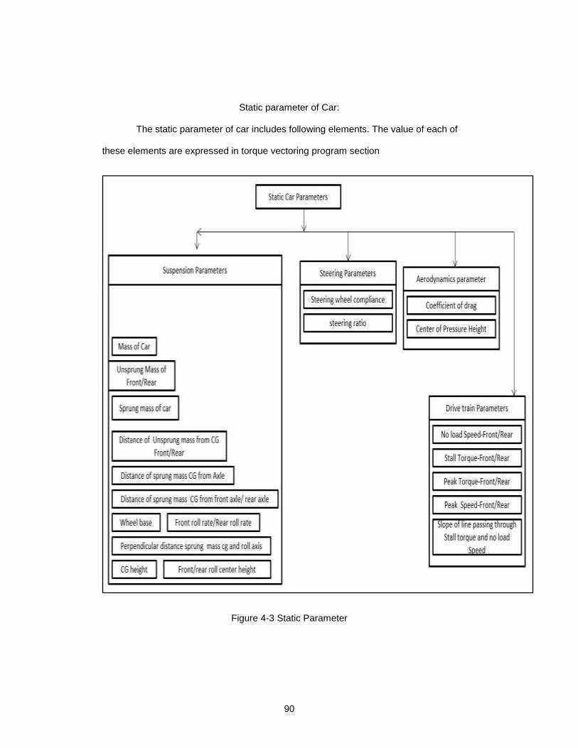
90
Static parameter of Car:
The static parameter of car includes following elements. The value of each of
these elements are expressed in torque vectoring program section
Figure 4-3 Static Parameter
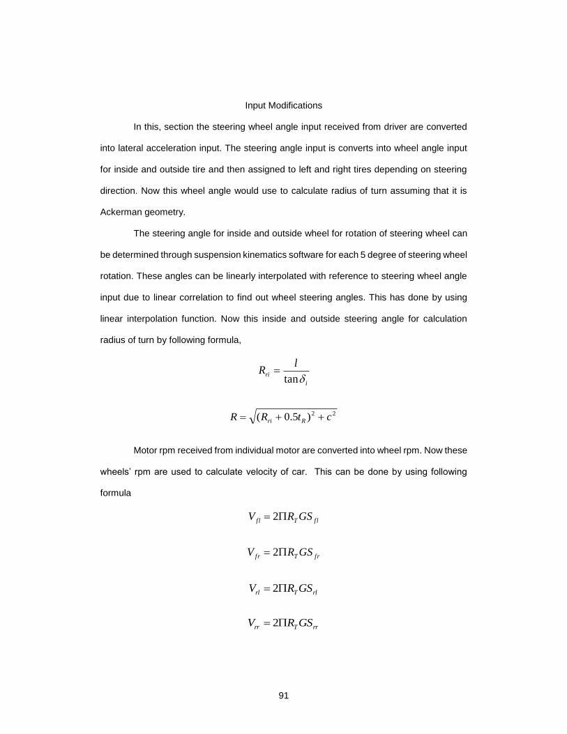
91
Input Modifications
In this, section the steering wheel angle input received from driver are converted
into lateral acceleration input. The steering angle input is converts into wheel angle input
for inside and outside tire and then assigned to left and right tires depending on steering
direction. Now this wheel angle would use to calculate radius of turn assuming that it is
Ackerman geometry.
The steering angle for inside and outside wheel for rotation of steering wheel can
be determined through suspension kinematics software for each 5 degree of steering wheel
rotation. These angles can be linearly interpolated with reference to steering wheel angle
input due to linear correlation to find out wheel steering angles. This has done by using
linear interpolation function. Now this inside and outside steering angle for calculation
radius of turn by following formula,
i
ri
lR
tan
22)5.0( ctRR Rri
Motor rpm received from individual motor are converted into wheel rpm. Now these
wheels’ rpm are used to calculate velocity of car. This can be done by using following
formula
f lTfl GSRV 2
frTfr GSRV 2
rlTrl GSRV 2
rrTrr GSRV 2

92
The average velocity of car can be calculated as follows
4
rrlrfrfl VVVVV
Now this calculated velocity and radius of turn are used to calculate, lateral acceleration
by following formula,
R
VAY
2
For left hand turn, the sign of lateral acceleration is set to be negative while for
right hand turn the sign of lateral acceleration is set to be positive. Also according to FSAE
rules, the car can perform regenerative braking below 5 KPH or 1.33 m/s the regenerative
brake position from driver is automatically set to be 0.
Calculation of Normal load on each wheel
Based on normal load equations derived in chapter 3, normal load on each wheel
are calculated based on formulas defined in section combined load calculation.

93
Calculation of Total driver requested torque:
Based on measured motor rpm combined with motor equation derived in chapter
2. The total torque calculated at each wheel can be calculated as follows .The equation
used for calculation of total driver requested torque is as follows.
Also in this formula if calculated
In case of throttle input from driver
𝑇𝑓𝑙 = −𝑇𝑝𝑒𝑎𝑘𝑓
𝑆𝑝𝑒𝑎𝑘𝑓
𝑆𝑓𝑙 + 𝑇𝑃 𝑇𝑝𝑒𝑎𝑘𝑓
𝑇𝑓𝑟 = −𝑇𝑝𝑒𝑎𝑘𝑓
𝑆𝑝𝑒𝑎𝑘𝑓
𝑆𝑓𝑟 + 𝑇𝑃 𝑇𝑝𝑒𝑎𝑘𝑓
𝑇𝑟𝑙 = −𝑇𝑝𝑒𝑎𝑘𝑟
𝑆𝑝𝑒𝑎𝑘𝑟
𝑆𝑟𝑙 + 𝑇𝑃 𝑇𝑝𝑒𝑎𝑘𝑟
𝑇𝑟𝑟 = −𝑇𝑝𝑒𝑎𝑘𝑟
𝑆𝑝𝑒𝑎𝑘𝑟rrS + 𝑇𝑃 𝑇𝑝𝑒𝑎𝑘𝑟
𝑇𝑟𝑒𝑞𝑢𝑒𝑠𝑡𝑒𝑑 = 𝑇𝑓𝑙 + 𝑇𝑓𝑟 + 𝑇𝑟𝑙 + 𝑇𝑟𝑟
Regen
max)( TSS
TT
Peak
Peak
𝑇𝑓𝑙 =𝑇𝑝𝑒𝑎𝑘𝑓
𝑆𝑝𝑒𝑎𝑘𝑓
𝑆𝑓𝑙 − 𝑅𝑃 𝑇𝑝𝑒𝑎𝑘𝑓

94
𝑇𝑓𝑟 =𝑇𝑝𝑒𝑎𝑘𝑓
𝑆𝑝𝑒𝑎𝑘𝑓
𝑆𝑓𝑟 − 𝑅𝑃 𝑇𝑝𝑒𝑎𝑘𝑓
𝑇𝑟𝑙 =𝑇𝑝𝑒𝑎𝑘𝑟
𝑆𝑝𝑒𝑎𝑘𝑟
𝑆𝑟𝑙 − 𝑅𝑃 𝑇𝑝𝑒𝑎𝑘𝑟
𝑇𝑟𝑟 =𝑇𝑝𝑒𝑎𝑘𝑟
𝑆𝑝𝑒𝑎𝑘𝑟rrS − 𝑅𝑃 𝑇𝑝𝑒𝑎𝑘𝑟
𝑇𝑟𝑒𝑞𝑢𝑒𝑠𝑡𝑒𝑑 = 𝑇𝑓𝑙 + 𝑇𝑓𝑟 + 𝑇𝑟𝑙 + 𝑇𝑟𝑟
Calculation of Vectored Torque
Now calculated torque in above scenario then used to calculate vectored torque
based upon the controller philosophy discussed in above section. This calculation of
vectored torque in algorithm represented as mode. The mode1 represents ‘3 differential
‘philosophy while Mode 2 represents 2 differential ‘philosophy. These modes can be
selected from E16 dash. Now the algorithm for calculation of vectored torque can be
represented as

95
Figure 4-4 Calculation of vectored torque algorithm1

96
Figure 4-5 Needs to be updated

97
Mode -1 – 3 Differential philosophy
In 3 differential mode, the total requested torque get distributed depending upon
the normal load on each wheel. This mode is default mode of operation for torque
vectoring controller on car. In this mode, the total driver requested torque gets distribute
across four wheels depending on percentage of normal load on each wheel with
reference to weight of car. For example, if one wheel has 20% of normal load to the
weight of car then that will receive 20% of total driver requested torque.
The transition from mode 1 to mode 2 can be done by changing toggle switch on
E-16’s dash.
𝑉𝑇𝑓𝑙 = 𝑇𝑟𝑒𝑞𝑢𝑒𝑠𝑡𝑒𝑑
𝑊𝑓𝑙
𝑊
𝑉𝑇𝑓𝑟 = 𝑇𝑟𝑒𝑞𝑢𝑒𝑠𝑡𝑒𝑑
𝑊𝑓𝑟
𝑊
𝑉𝑇𝑟𝑙 = 𝑇𝑟𝑒𝑞𝑢𝑒𝑠𝑡𝑒𝑑
𝑊𝑟𝑙
𝑊
𝑉𝑇𝑟𝑟 = 𝑇𝑟𝑒𝑞𝑢𝑒𝑠𝑡𝑒𝑑
𝑊𝑟𝑟
𝑊
Now this 3 differential philosophy represented by,
Mode-2- 2 Differential philosophy
In case of 2 differential philosophy, the distributed torque on each wheel is
depends upon total weight and requested torque from each axle. The torque requested
from one axle does not get transferred to another axle. The total driver requested torque
from axle get distributed depending on amount percentage of normal load on wheel with
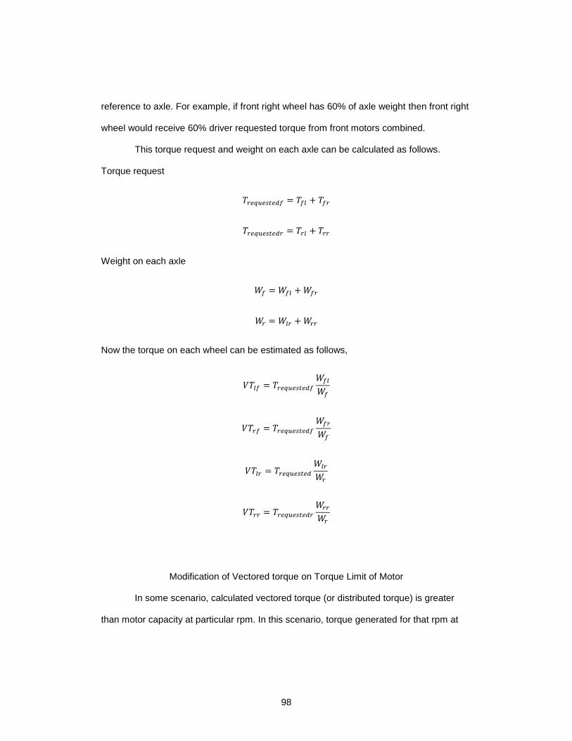
98
reference to axle. For example, if front right wheel has 60% of axle weight then front right
wheel would receive 60% driver requested torque from front motors combined.
This torque request and weight on each axle can be calculated as follows.
Torque request
𝑇𝑟𝑒𝑞𝑢𝑒𝑠𝑡𝑒𝑑𝑓 = 𝑇𝑓𝑙 + 𝑇𝑓𝑟
𝑇𝑟𝑒𝑞𝑢𝑒𝑠𝑡𝑒𝑑𝑟 = 𝑇𝑟𝑙 + 𝑇𝑟𝑟
Weight on each axle
𝑊𝑓 = 𝑊𝑓𝑙 + 𝑊𝑓𝑟
𝑊𝑟 = 𝑊𝑙𝑟 + 𝑊𝑟𝑟
Now the torque on each wheel can be estimated as follows,
𝑉𝑇𝑙𝑓 = 𝑇𝑟𝑒𝑞𝑢𝑒𝑠𝑡𝑒𝑑𝑓
𝑊𝑓𝑙
𝑊𝑓
𝑉𝑇𝑟𝑓 = 𝑇𝑟𝑒𝑞𝑢𝑒𝑠𝑡𝑒𝑑𝑓
𝑊𝑓𝑟
𝑊𝑓
𝑉𝑇𝑙𝑟 = 𝑇𝑟𝑒𝑞𝑢𝑒𝑠𝑡𝑒𝑑
𝑊𝑙𝑟
𝑊𝑟
𝑉𝑇𝑟𝑟 = 𝑇𝑟𝑒𝑞𝑢𝑒𝑠𝑡𝑒𝑑𝑟
𝑊𝑟𝑟
𝑊𝑟
Modification of Vectored torque on Torque Limit of Motor
In some scenario, calculated vectored torque (or distributed torque) is greater
than motor capacity at particular rpm. In this scenario, torque generated for that rpm at

99
100% duty cycle is to be calculated and this torque is compared with vectored torque. If
vectored torque value is greater than calculated value, vectored torque value is set to be
calculated value. These values can be calculated as follows
In case of throttle input from driver
𝑇𝑓𝑙100 = −𝑇𝑝𝑒𝑎𝑘𝑓
𝑆𝑝𝑒𝑎𝑘𝑓
𝑆𝑓𝑙 + 𝑇𝑝𝑒𝑎𝑘𝑓
𝑇𝑓𝑟100 = −𝑇𝑝𝑒𝑎𝑘𝑓
𝑆𝑝𝑒𝑎𝑘𝑓
𝑆𝑓𝑟 + 𝑇𝑝𝑒𝑎𝑘𝑓
𝑇𝑙𝑟100 = −𝑇𝑝𝑒𝑎𝑘𝑟
𝑆𝑝𝑒𝑎𝑘𝑟
𝑆𝑙𝑟 + 𝑇𝑝𝑒𝑎𝑘𝑟
𝑇𝑟𝑟100 = −𝑇𝑝𝑒𝑎𝑘𝑟
𝑆𝑝𝑒𝑎𝑘𝑟rrS + 𝑇𝑝𝑒𝑎𝑘𝑟
Regen
𝑇𝑓𝑙100 =𝑇𝑝𝑒𝑎𝑘𝑓
𝑆𝑝𝑒𝑎𝑘𝑓
𝑆𝑓𝑙 − 𝑇𝑝𝑒𝑎𝑘𝑓
𝑇𝑓𝑟100 =𝑇𝑝𝑒𝑎𝑘𝑓
𝑆𝑝𝑒𝑎𝑘𝑓
𝑆𝑓𝑟 − 𝑇𝑝𝑒𝑎𝑘𝑓
𝑇𝑟𝑙100 =𝑇𝑝𝑒𝑎𝑘𝑟
𝑆𝑝𝑒𝑎𝑘𝑟
𝑆𝑟𝑙 − 𝑇𝑝𝑒𝑎𝑘𝑟
𝑇𝑟𝑟100 =𝑇𝑝𝑒𝑎𝑘𝑟
𝑆𝑝𝑒𝑎𝑘𝑟
𝑆𝑟𝑟 − 𝑇𝑝𝑒𝑎𝑘𝑟

100
If the throttle pedal is pressed, these calculated values would be used to
compare with vectored torque. If vectored torque value for wheel is greater than
calculated value. The vectored torque would be equal to calculated values otherwise it
would remain same.
If regen pedal is pressed, if vectored torque value is less than calculated value,
the vectored torque would be equal to calculated values otherwise it would remain same.
This happens due to negative sign on regenerative braking values.

101
Calculation of Throttle or Regen Position
Now E-16’s motor controller does not have any current measurement device on
them, they only recognize the duty cycle input. So, it is required to convert vectored torque
into throttle position (positive duty cycle) or regenerative brake position (negative duty
cycle) for application of motor torque. This kind of mechanism allow motor controllers to
apply appropriate amount of voltage to generate vectored torque.
It is calculating throttle position or regen position, with the help of registered
controller speed and calculated vectored torque.
.The E-16’s motor controller design is open loop motor controller. These motor
controllers always required to state throttle (positive duty cycle) and regen (negative duty
cycle) for their operation. When driver is requesting torque through throttle pedal, algorithm
calculates throttle position and set regen position to zero. Similarly, when driver is
requesting braking torque through regen pedal, this algorithm calculates regen position
and set throttle position to zero. This calculation uses following formulae.
In case of throttle request:
ƛ𝑡ℎ𝑟𝑜𝑡𝑡𝑙𝑒𝑓𝑙 =
(𝑉𝑇𝑓𝑙 − (−𝑇𝑝𝑒𝑎𝑘𝑓
𝑆𝑝𝑒𝑎𝑘𝑓 ) 𝑆𝑓𝑙 )
𝑇𝑝𝑒𝑎𝑘𝑓
ƛ𝑡ℎ𝑟𝑜𝑡𝑡𝑙𝑒𝑓𝑟 =
(𝑉𝑇𝑓𝑙 − (−𝑇𝑝𝑒𝑎𝑘𝑓
𝑆𝑝𝑒𝑎𝑘𝑓 ) 𝑆𝑓𝑟 )
𝑇𝑝𝑒𝑎𝑘𝑓
ƛ𝑡ℎ𝑟𝑜𝑡𝑡𝑙𝑒𝑟𝑙 =
(𝑉𝑇𝑙𝑟 − (−𝑇𝑝𝑒𝑎𝑘𝑟
𝑆𝑝𝑒𝑎𝑘𝑟 ) 𝑆𝑙𝑟 )
𝑇𝑝𝑒𝑎𝑘𝑟
ƛ𝑡ℎ𝑟𝑜𝑡𝑡𝑙𝑒𝑟𝑟 =
(𝑉𝑇𝑟𝑟 − (−𝑇𝑝𝑒𝑎𝑘𝑟
𝑆𝑝𝑒𝑎𝑘𝑟 ) 𝑆𝑟𝑟 )
𝑇𝑝𝑒𝑎𝑘𝑟
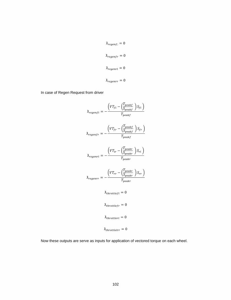
102
ƛ𝑟𝑒𝑔𝑒𝑛𝑓; = 0
ƛ𝑟𝑒𝑔𝑒𝑛𝑓𝑟 = 0
ƛ𝑟𝑒𝑔𝑒𝑛𝑟𝑙 = 0
ƛ𝑟𝑒𝑔𝑒𝑛𝑟𝑟 = 0
In case of Regen Request from driver
ƛ𝑟𝑒𝑔𝑒𝑛𝑓𝑙 = −
(𝑉𝑇𝑓𝑙 − (𝑇𝑝𝑒𝑎𝑘𝑓
𝑆𝑝𝑒𝑎𝑘𝑓 ) 𝑆𝑓𝑙 )
𝑇𝑝𝑒𝑎𝑘𝑓
ƛ𝑟𝑒𝑔𝑒𝑛𝑓𝑟 = −
(𝑉𝑇𝑓𝑟 − (𝑇𝑝𝑒𝑎𝑘𝑓
𝑆𝑝𝑒𝑎𝑘𝑓 ) 𝑆𝑓𝑟 )
𝑇𝑝𝑒𝑎𝑘𝑓
ƛ𝑟𝑒𝑔𝑒𝑛𝑟𝑙 = −
(𝑉𝑇𝑙𝑟 − (𝑇𝑝𝑒𝑎𝑘𝑟
𝑆𝑝𝑒𝑎𝑘𝑟 ) 𝑆𝑟𝑙 )
𝑇𝑝𝑒𝑎𝑘𝑟
ƛ𝑟𝑒𝑔𝑒𝑛𝑟𝑟 = −
(𝑉𝑇𝑟𝑟 − (𝑇𝑝𝑒𝑎𝑘𝑟
𝑆𝑝𝑒𝑎𝑘𝑟 ) 𝑆𝑟𝑟 )
𝑇𝑝𝑒𝑎𝑘𝑟
ƛ𝑡ℎ𝑟𝑜𝑡𝑡𝑙𝑒𝑓𝑙 = 0
ƛ𝑡ℎ𝑟𝑜𝑡𝑡𝑙𝑒𝑓𝑟 = 0
ƛ𝑡ℎ𝑟𝑜𝑡𝑡𝑙𝑒𝑟𝑙 = 0
ƛ𝑡ℎ𝑟𝑜𝑡𝑡𝑙𝑒𝑙𝑟𝑟 = 0
Now these outputs are serve as inputs for application of vectored torque on each wheel.
103
Torque Vectoring Controller Program :
The torque vectoring controller program logic has written in MATLAB , then it is use to
generate Simulink function with shown input and output in Figure 4-1 to facilitate generation
C code through code generation . The program is written in descriptive language instead
of symbols for ease of understanding and future development of this program. This
program has attached in Appendix C
104
Chapter 5 Torque Vectoring Controller Testing and Conversion
Introduction:
This chapter will provide detail procedure for testing of Torque vectoring controller program
has discussed. The torque-vectoring program consist of 10 inputs and 8 outputs, this
makes it very difficult to find out error at any particular instance. However, there are definite
range of each particular input.
Torque vectoring controller should provide more torque on rear wheels during longitudinal
acceleration while performing in mode 1 (3- differential philosophy). Also torque at front
two wheels (left and right) must be identical and torque on rear two wheels (left and right)
must be identical. Further, it should provide a regenerative torque on front wheels during
longitudinal deceleration (braking). In addition to that, front two wheel must have identical
torque and it should apply same torque for rear two wheels. In mode 2 (2 differential
philosophy) controller should apply equal torque on left and right wheels at each axle and
it will always apply more torque on rear wheels, as rear motors has more torque producing
capacity.
When car is taking right turn, torque-vectoring controller should apply more torque on left
wheels than that of right wheels. When car is taking a left turn, torque-vectoring controller
should apply more torque right wheel and less on left wheels. The amount of torque applied
on each wheel depends on the amount of normal load and torque-vectoring philosophy is
used .In addition to above torque vectoring controller should produce equal output during
left hand and right hand turn for same lateral acceleration.
As, it is very difficult to test all of the above philosophies and realizing outputs for different
combinations of input. For this purpose, the range of input has decided. This range of input
then used to define test matrix for testing of controller program. The output of these test

105
matrixes are plotted on graph for easy error detection, asymmetry of operation and wrong
outputs
As the output of this program are throttle position (drive duty cycle) or regenerative brake
position (regenerative duty cycle) for motor controller, the output of this programs would
always lie in-between 0-100%
As described in earlier chapter, this program is going to run on supervisor board (micro-
controller). It is very necessary to convert this program into C code. This program can be
converted to C code by manually or with the help of C-code generator tool in MATLAB
Simulink. The manually converted C- code would be efficient and it would have less
processing time. However, manual c conversion limits increases time for modification of
program. Though manually generated C code is efficient, it takes very large time to modify
the code. In addition, the processing power installed on E-16 is more than sufficient for
running torque-vectoring program, it has decided to use ‘C code generator’ tool for ease of
controller program development and testing. The use of c code generator to generate C
code has discussed at end of this chapter.
Range of Input parameters :
Torque vectoring controller program has the 10 input parameters, the range of these
parameters depends upon steering kinematics design, powertrain design, tires and torque
vectoring philosophies. This range of input parameter are also used in upstream vehicle
state monitoring program for detection of sensor failures. If the range of values read by
vehicle monitoring program were outside of defined range for more than 2 seconds, the
sensor would declared to be dead. Further, there are more complex algorithms are involved
to detect this sensor failure in upstream program but they are not part of this thesis study.
In addition, the resolution of data recording has been decided for calculation of torque
vectoring program

106
Range of parameter:
Steering Angle:
The data collected from kinematics design of E-16’ steering geometry shows that the
steering wheel angle would lie in between -105 degree to 105 degree during normal mode
of operation. Any value read above 110 degree would be declare as sensor failure.
However, any value read in-between 105-110 degree declared as 105 degree by upstream
program. These 5 degrees of tolerance has given for incidental error occurring in sensor
data filtering. Therefore, testing range of steering wheel angle has decided as -105 to 105
Throttle Position and Regen brake Position: -
The throttle position and regenerative brake positions are detected by potentiometers
installed on respective pedals. These values of regenerative brake and throttle position
varies in-between 0-100% during normal mode of operation. Any value read below -5 % or
above 105 % declared as potentiometer failure, in upstream program and car will
automatically will turn off high voltage system. The value read in between 0 to -5 or 100-
105 would be declared as 0 or 100 % by upstream program. Therefore, testing range for
throttle and regenerative brake position has decided as 0-100%

107
Motor RPM
As described in chapter 2, all the motors are limited to 15000 rpm for longer bearing life.
Therefore, the testing range for motor rpm has decided as 0-15000 rpm for each motor.
Longitudinal acceleration:
As E-16’s motors has capability produce instantaneous torque at the start. The acceleration
of this car is traction limited (tire limited). From the careful study of tire data, it has found
that this tire would able to support 1.5g’s longitudinal acceleration and braking. The
program has to compatible to wide range of acceleration input Therefore, the range of
longitudinal acceleration has selected as -19.62 m/s2 to 19.62 m/s2 (-2g’s to 2 g)for testing.
The E-16’s accelerometer automatically generates the error signal during accelerometer
failure; no special algorithm is required to detect accelerometer failure.
Lateral acceleration
The study of aerodynamics, suspension and tire characteristics at various speed, the E-
16’s would able to pull 2g’s of lateral acceleration. Therefore, lateral range of acceleration
has selected as -19.62 m/s2 to 19.62m/s2 (-2g’s to 2g’s)for testing.
108
Test Matrix
The test matrix of the car has decided to test working of torque vectoring controller within
the range of input parameters. In this test matrix has set up in 3 levels.
In level 1, the car is assumed to be static, so all rpm of motor are set to be 0 rpm and the
all other inputs are varies one by one to realize outputs of torque vectoring controller while
car is standing still. It test the response of torque vectoring controller during coasting.
In level 2, it assumes that car is running at full speed and all other inputs has varied in their
range to realize response of torque vectoring controller. This way response of a car while
running at top speed has realized.
In level 3, It assumes that car is running at average track speed of FSAE car, 30 mph. This
can be done by setting up all motor speed at 5000 rpm and all other inputs are varies in
between their range to realize response of car. In this level, the outputs of torque vectoring
controllers are tested for left and right hand turn to check the symmetry of operation. In
addition, the symmetry of operation has checked for longitudinal acceleration.

109
Table 5-1 Torque Vectoring Controller Program Test Matrix
Throttle Regen Steering Ax Ay FL rpm FR rpm RL rpm RR rpm Notes
Level_1_1 X 0 0 0 0 0 0 0 0
Level_1_2 0 X 0 0 0 0 0 0 0
Level_1_3 0 0 X 0 0 0 0 0 0
Level_1_4 0 0 0 X 0 0 0 0 0
Level_1_5 0 0 0 0 X 0 0 0 0
Level_1_6 0 0 0 0 0 X X X X All Wheel Speeds
Same Level_2_1 X 0 0 0 0 15000 15000 15000 15000 All Wheel Speeds
Same Level_2_2 0 X 0 0 0 15000 15000 15000 15000 All Wheel Speeds
Same Level_2_3 0 0 X 0 0 15000 15000 15000 15000 All Wheel Speeds
Same Level_2_4 0 0 0 X 0 15000 15000 15000 15000 All Wheel Speeds
Same Level_2_5 0 0 0 0 X 15000 15000 15000 15000 All Wheel Speeds
Same Level_3_1 X 0 0 0 0 X X X X All Wheel Speeds
Same Level_3_2 0 X 0 0 0 X X X X All Wheel Speeds
Same Level_3_3 X 0 - 105 to 0 0 0 5000 5000 5000 5000 All Wheel Speeds
Same Level_3_4 X 0 0 to105 0 0 5000 5000 5000 5000 All Wheel Speeds
Same Level_3_5 X 0 0 -2 to 0 0 5000 5000 5000 5000 All Wheel Speeds
Same Level_3_6 X 0 0 0 to 2 0 5000 5000 5000 5000 All Wheel Speeds
Same Level_3_7 X 0 0 0 -2 to 0 5000 5000 5000 5000 All Wheel Speeds
Same Level_3_8 X 0 0 0 0 to 2 5000 5000 5000 5000 All Wheel Speeds
Same
The MATLAB program has developed for testing of torque vectoring controller program.
This test program calls a torque vectoring controller program as function and swept the
inputs as mentioned in above test matrix. In addition, it plots following outputs from this
program The program for testing level _3_7 is attached in annex A and it can be modified
to test any above level test, just by changing the input values.
drive requested throttle position vs torque vectored throttle position vs swept
input –each wheel
driver requested regen position vs torque vectored throttle position vs swept
input-each wheel
input throttle position vs motor torque (vectored and driver requested) vs swept
input- each wheels

110
input throttle position vs motor torque (vectored and driver requested) vs swept
input- All wheels
These graphs give idea about the working of torque vectoring controller program over the
range of swept input and this helps in analyzing controller response to one input.
Once the response for each input works as expected, it is better to assume that in any
combination of above input this controller would able to produce desired effects.
The output of torque vectoring controller for above mention level as follows.

111
Level Testing Output
These different levels has tested for two strategies.. The nomenclature of figure attached
is as Level_1_1_Mode_Wheel location response (output). Mode 1 represents the 3
differential strategy in level testing program while Mode 2 represents the 2 differential
strategy. The results are represented to demonstrate performance of torque vectoring
controller.
If legends are required to read, these graphs are represented only on front left motors.
Otherwise, it can be assumed to be consistent with figure title.
Level 1 Testing
FSAE cars are not allowed to do regeneration below 5 kph and reverse is not allowed. The
response of torque vectoring controller program should be 0% regenerative duty that has
tested in level_1_2. As described earlier, the testing done in level_ 1_3 level_1_4 Level
_1_5 and level_1_6 is static testing to make sure that ,torque vectoring program does not
distribute torque statically even if driver is requesting torque from the throttle pedal . Not all
of these levels are important to represent here.
However, the level 1_1 is important to state, as it would provide information about torque
vectoring controller program output at static when driver would press throttle pedal. The
responses of torque vectoring controller in level 1_1_Mode 1 are represented below.

112
In mode 1, the values of torque vectored throttle position would be greater than driver
throttle position as statically car is front bias. The regenerative response would be null due
to throttle pedal input. In addition, the values of vectored torque for front motors should
greater than driver requested torque and rear motors.
In mode 2 torque vectoring controller does not distributes torque longitudinally so input
throttle equal to vectored throttle. In addition, values for driver requested torque would be
equal to vectored torque for all motors

113
Figure 5-1 Level_1_1_Mode 1_FL _Throttle
Figure 5-2 Level_1_1_mode 1_FR _throttle

114
Figure 5-3 Level_1_1_mode 1_RL _throttle
Figure 5-4 Level _1_1_mode1_RR_throttle

115
Figure 5-5 Level _1_1_mode1_FL_regen
Figure 5-6 Level _1_1_mode1_FR_regen

116
Figure 5-7 Level _1_1_mode1_RL_Regen
Figure 5-8 Level _1_1_mode1_RR_Regen

117
Figure 5-9 Level _1_1_mode1_FL_Torque Response
Figure 5-10 Level _1_1_mode1_FR_Torque Response

118
Figure 5-11 Level _1_1_mode1_RL_Torque Response
Figure 5-12 Level _1_1_mode1_RR_Torque Response

119
Figure 5-13 Level_1_1_Mode 2_FL _Throttle Response
Figure 5-14 Level_1_1_Mode 2_FL _Throttle Response

120
Figure 5-15 Level_1_1_Mode 2_RL _Throttle Response
Figure 5-16 Level_1_1_Mode 2_RR _Throttle Response

121
Figure 5-17 Level_1_1_Mode 2_FL _Regen
Figure 5-18 Level_1_1_Mode 2_FR _Regen

122
Figure 5-19 Level_1_1_Mode 2_RL_Regen
Figure 5-20 Level_1_1_Mode 2_RR_Regen

123
Figure 5-21 Level _1_1_mode2_FL_Torque Response
Figure 5-22 Level _1_1_mode2_FR_Torque Response

124
Figure 5-23 Level _1_1_mode2_RL_Torque Response
Figure 5-24 Level _1_1_mode2_RL_Torque Response

125
Level 2 Testing:
In level 2, it assumes that car is running at top speed and test mentioned in level 2 except
of level 2_1 assumes that, driver is coasting at high speed. As mentioned earlier, while
coasting torque vectoring controller program does not produce any torque vectoring, so it
is not worth mentioning about this responses.
However, it is important to know torque vectoring program response when car is moving at
constant velocity at top speed.
As from the analysis of front motor models, it can be concluded that front motors would not
able to produce any torque until 68% throttle input at 15000 rpm. Therefore, the torque
vectoring controller should produce null output till 68% throttle. It supposed to produce
similar output for front wheels and rear wheels, as car is not turning. In addition to that
throttle input is there means there will null output for regen position these responses of
torque vectoring controller has tested below
Level_ 2_1 Testing
The level_2_1 tests the response of torque vectoring controller to respond constant velocity
scenario.
In mode 1, the value of vectored torque would be null until 68% throttle and the values of
vectored throttle position would be greater than driver requested throttle position.
As controller program is receiving throttle input, the regenerative response of program will
be null.
This test assumes that car is running at constant velocity, If throttle position is less than
68% then controller program would calculate vectored torque as equal to driver requested
torque as null due to physical motor limitations. At the end program will dictate that throttle
position is null (or 0) for each motor controller. However if input throttle is greater than 68%
then Torque would be distributed depending on mode.

126
In mode1, if throttle input is less than 68% then driver requested torque would be equivalent
to vectored torque. However, this application of torque is not possible physically so it would
be avoided by program automatically. If throttle is greater than 68% more torque would be
applied to front motors, as car is more front weight bias. This torque would be same for
front motors (left and right) and rear motors (left and right). The regen output would be null
in this scenario.
In mode 2, If throttle output of the program would have similar nature to mode 1. If throttle
input is less than 68% then vectored torque, vectored throttle and driver requested torque
would be null. If throttle input is greater than 68% then driver requested torque would be
equivalent to vectored torque. The more torque would be applied to rear motors because
rear motors produce the more torque at same speed and throttle than front motors. The
regenerative response would be null as throttle input is present.

127
Figure 5-25 Level_2_1_Mode1_FL_Throttle Response
Figure 5-26 Level_2_1_Mode1_FR_Throttle Response

128
Figure 5-27 Level_2_1_Mode1_RL_Throttle Response
Figure 5-28 Level_2_1_Mode1_RR_Throttle Response

129
Figure 5-29 Level_2_1_Mode1_FL_Regen Response
Figure 5-30 Level_2_1_Mode1_FR_Regen Response

130
Figure 5-31 Level_2_1_Mode1_RL_Regen Response
Figure 5-32 Level_2_1_Mode1_RR_Regen Response

131
The controller is providing more torque to front motors during due to front weight bias of
car so controller response is acceptable
Figure 5-33 Level_2_1_Mode1_FL-Torque Response
Figure 5-34 Level_2_1_Mode1_FR-Torque Response

132
Figure 5-35 Level_2_1_Mode1_RL-Torque Response
Figure 5-36 Level_2_1_Mode1_RR-Torque Response

133
Figure 5-37 Level_2_1_Mode2_FL-Throttle Response
Figure 5-38 Level_2_1_Mode2_FR-Throttle Response

134
Figure 5-39 Level_2_1_Mode2_RL-Throttle Response
Figure 5-40 Level_2_1_Mode2_RR-Throttle Response

135
Figure 5-41 Level_2_1_Mode2_FL-Regen Response
Figure 5-42 Level_2_1_Mode2_FR-Regen Response

136
Figure 5-43 Level_2_1_Mode2_RL-Regen Response
Figure 5-44 Level_2_1_Mode2_RR-Regen Response
The controller response is as expected, so it is acceptable

137
Figure 5-45 Level_2_1_Mode2_FL-Torque Response
Figure 5-46 Level_2_1_Mode2_FR-Torque Response

138
Figure 5-47 Level_2_1_Mode2_RL-Torque Response
Figure 5-48 Level_2_1_Mode2_RR-Torque Response

139
Level 2_2 Testing.
The regenerative pedal input is being swept in level 2_2. This thesis study assumed that,
the motors would have similar torque speed characteristic in regenerative characteristic a
as that of throttle. Therefore, torque-vectoring controller would produce similar response in
regenerative mode as that of throttle response in level 2_1. The throttle response of
program would be null due to regen input. The amount of torque applied to each wheel
depending on the mode in which car is operating. The torque produced by motors would
be negative due to regen input. Like mentioned in level_2_1 motors would not able to
produce any regenerative torque below 68% regen input. . If regen input is less than 68%
then vectored torque, driver requested torque and vectored regen position would be null.
In mode 1, the throttle response would be null The regenerative response would be
equivalent to throttle response in level_2_1 in mode 1.The torque received by front motors
would be higher than rear motors due to front weight bias. The torque received by front
motors (left and right) as well as rear motors (left and right) would be identical.
In mode 2 the throttle response would be null. The input regenerative position would be
equivalent to response of throttle in level_2_1 in mode 2. The vectored torque received
by rear motor would be higher due to their higher power rating. In addition to that, driver
requested torque would be similar to vectored torque, as controller does not able to
distribute torque except for turning scenario.
The response torque-vectoring controller for level 2_2 would be as follow
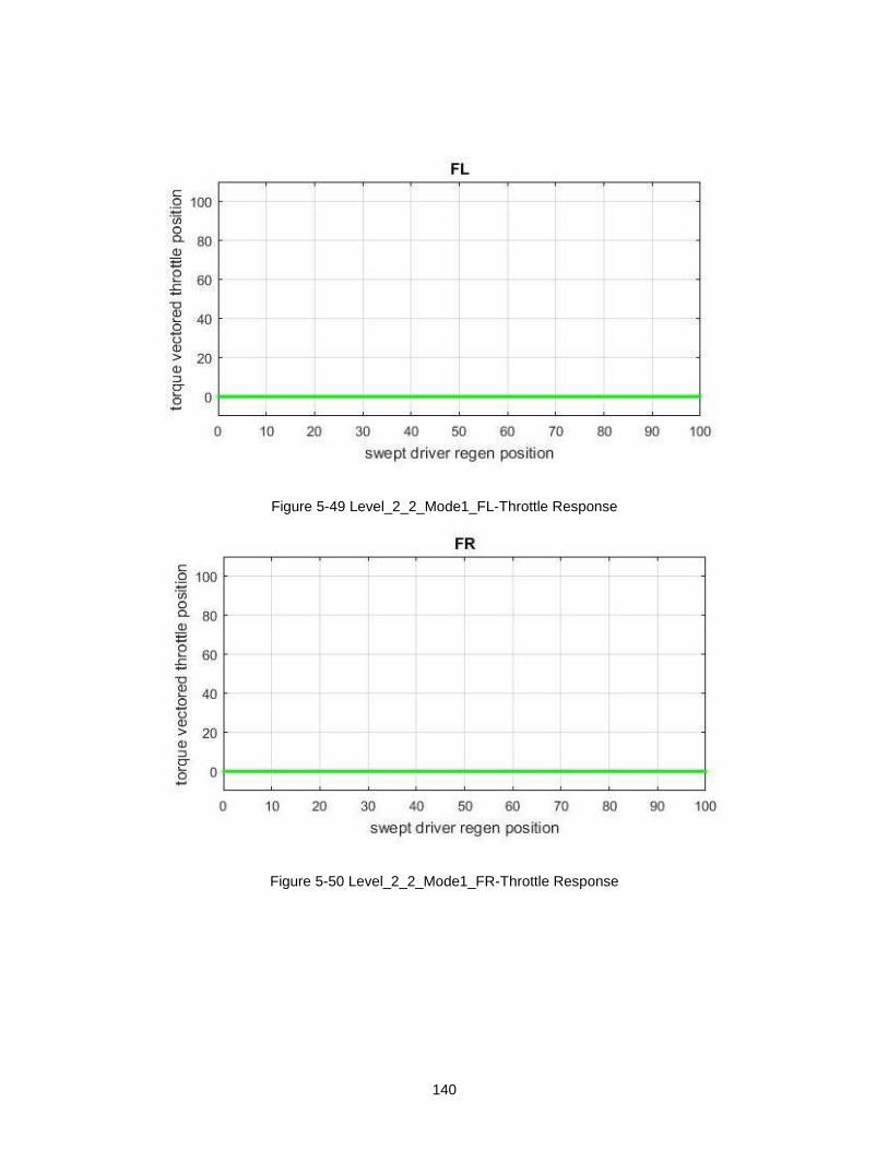
140
Figure 5-49 Level_2_2_Mode1_FL-Throttle Response
Figure 5-50 Level_2_2_Mode1_FR-Throttle Response

141
Figure 5-51 Level_2_2_Mode1_RL-Throttle Response
Figure 5-52 Level_2_2_Mode1_RR-Throttle Response

142
Figure 5-53 Level_2_2_Mode1_FL-Regen Response
Figure 5-54 Level_2_2_Mode1_FR-Regen Response

143
Figure 5-55 Level_2_2_Mode1_RL-Regen Response
Figure 5-56 Level_2_2_Mode1_RR-Regen Response

144
Figure 5-57 Level_2_2_Mode1_FL-Torque Response
Figure 5-58 Level_2_2_Mode1_FR-Torque Response

145
Figure 5-59 Level_2_2_Mode1_RL-Torque Response
Figure 5-60 Level_2_2_Mode1_RR-Torque Response

146
Figure 5-61 Level_2_2_Mode2_FL-Throttle Response
Figure 5-62 Level_2_2_Mode2_FL-Throttle Response

147
Figure 5-63 Level_2_2_Mode2_RL-Throttle Response
Figure 5-64 Level_2_2_Mode2_RR-Throttle Response

148
The response of torque vectoring controller to regenerative position is as explained
above. Therefore, these results are acceptable t
Figure 5-65 Level_2_2_Mode2_FL-Regen Response
Figure 5-66 Level_2_2_Mode2_FR-Regen Response

149
Figure 5-67 Level_2_2_Mode2_RL-Regen Response
Figure 5-68 Level_2_2_Mode2_RR-Regen Response

150
Figure 5-69 Level_2_2_Mode2_FL-Torque Response
Figure 5-70 Level_2_2_Mode2_FR-Torque Response

151
Figure 5-71 Level_2_2_Mode2_RLTorque Response
Figure 5-72 Level_2_2_Mode2_RRTorque Response

152
Level 3 Testing
In level, 3 testing motors are assumed to be running at 5000 rpm that translates into
average speed of FSAE car on track (approx. 30 mile/hr.). The study of motor models
presented in chapter 2 shows that at this speed front and rear motors would not able to
produce any torque below 23% throttle input due to physical limitation of motors. This can
be observed throughout all the level 3 tests.
The testing conditions described for level_3_1 and level_3_2 are equivalent to test
conditions described in level_2_1 and level_2_2 but at different speed, so it is not
worthwhile to study these responses here.
From earlier studied responses, it is very easy to conclude that; torque vectoring controller
program would capable to produce accurate throttle position and regenerative position
output for motor controller. In addition, it can be concluded that it is easy to study controller
response from torque response of controller.
Level 3_3 and Level 3_4
The test set up described in level 3_3 and level 3_4 describes torque-vectoring controller
based on steering input and driver throttle input at given speed. The torque responses are
studied for these levels in both modes. These responses would supposed to show increase
in left and right torque biasing as steering wheel angle is increasing , radius of turn
decreases and lateral acceleration approximated by torque vectoring program increases.

153
Level 3_3 Testing:
The level_3_3 response represents the torque vectoring controller response to steering
and throttle input. In level_ 3_3 car assumed to be making left turn. As steering wheel angle
increases, radius of turn decreases and calculated value of lateral acceleration increases.
This increase in calculated value of lateral acceleration results into more torque on right
side wheels.
In mode 1, as there is not longitudinal acceleration, Front wheels would receive more
vectored torque. In addition to that, right side wheel at front and rear axle would receive
more torque than left side wheels as car is making left hand turn. The negative values of
vectored torque on front left wheel represents the wheel lift scenario.
In mode 2, the lateral torque distribution would have nature similar to mode 1 . However,
rear wheels would receive more torque due to higher power rating.

154
Figure 5-73 Level_3_3_Mode1_FL_Torque Response
Figure 5-74 Level_3_3_Mode1_FR_Torque Response

155
Figure 5-75 Level_3_3_Mode1_RL_Torque Response
Figure 5-76 Level_3_3_Mode1_RR_Torque Response

156
Figure 5-77 Level_3_3_Mode2_FL_Torque Response
Figure 5-78 Level_3_3_Mode2_FR_Torque Response

157
Figure 5-79 Level_3_3_Mode2_RL_Torque Response
Figure 5-80 Level_3_3_Mode2_RR_Torque Response

158
Level 3_4
The level_3_4 response represents the torque vectoring controller response to steering
and throttle input. In level_3_4 car assumed to be making right turn. The lateral
acceleration would increase with increased steering input as explained in level_3_3 testing
but this time direction of lateral acceleration would be reversed. This increase in calculated
value of reversed lateral acceleration results into more torque on left side wheels.
In mode 1, as there is not longitudinal acceleration, Front wheels would receive more
vectored torque. In addition to that, left side wheel at front and rear axle would receive
more torque than right side wheels as car is making right hand turn.
In mode 2, the lateral torque distribution would have nature similar to mode 1, and rear
wheels would receive more torque due to higher power rating.

159
Figure 5-81 Level_3_4_Mode1_FL_Torque Response
Figure 5-82 Level_3_4_Mode1_FR_Torque Response

160
Figure 5-83 Level_3_4_Mode1_RL_Torque Response
Figure 5-84 Level_3_4_Mode1_RR_Torque Response

161
Figure 5-85 Level_3_4_Mode2_FL_Torque Response
Figure 5-86 Level_3_4_Mode2_FR_Torque Response

162
Figure 5-87 Level_3_4_Mode2_RL_Torque Response
Figure 5-88 Level_3_4_Mode1_RR_Torque Response

163
Level 3_5 and Level 3_6
The level_3_5 and level_3_6 test setups are testing torque vectoring controller program
response to longitudinal acceleration. The level 3_5 tests the deceleration scenario while
level 3_6 tests the acceleration scenario. The torque responses for these levels are studied
for mode 1 and mode 2.
Level 3_5 Testing
From below graphs represented for level 3_5_Mode1 .the vectored torque on front tire
should increase as a longitudinal acceleration increases approaches towards -2g’s and
torque on rear wheel goes on decreasing.
While in mode level 3_5_Mode 2 , driver requested torque from each wheel would be equal
to torque vectored torque. As mode 2 only distributes the torque in lateral acceleration. The
response would be similar to described in level 2_1_Mode 2 testing. Therefore, this
response is not discussed below.

164
Figure 5-89 Level_3_5_1_Mode1_FL_Torque Response
Figure 5-90 Level_3_5_1_Mode1_FR_Torque Response

165
Figure 5-91 Level_3_5_1_Mode1_RL_Torque Response
Figure 5-92 Level_3_5_1_Mode1_RR_Torque Response

166
Level 3_6 Testing
The car is accelerating from 0 to 2 g’s has described in level_3_6 testing. The vectored
torque on front tires should decrease and torque on rear tires should increase during
longitudinal acceleration. Because load on rear tires increases during longitudinal
acceleration.
In mode 2, vectored torque would be same as drive requested torque because mode 2
would able to distribute torque only in lateral directions.
The testing output for level_3_6_Mode 1 would look like as follows.
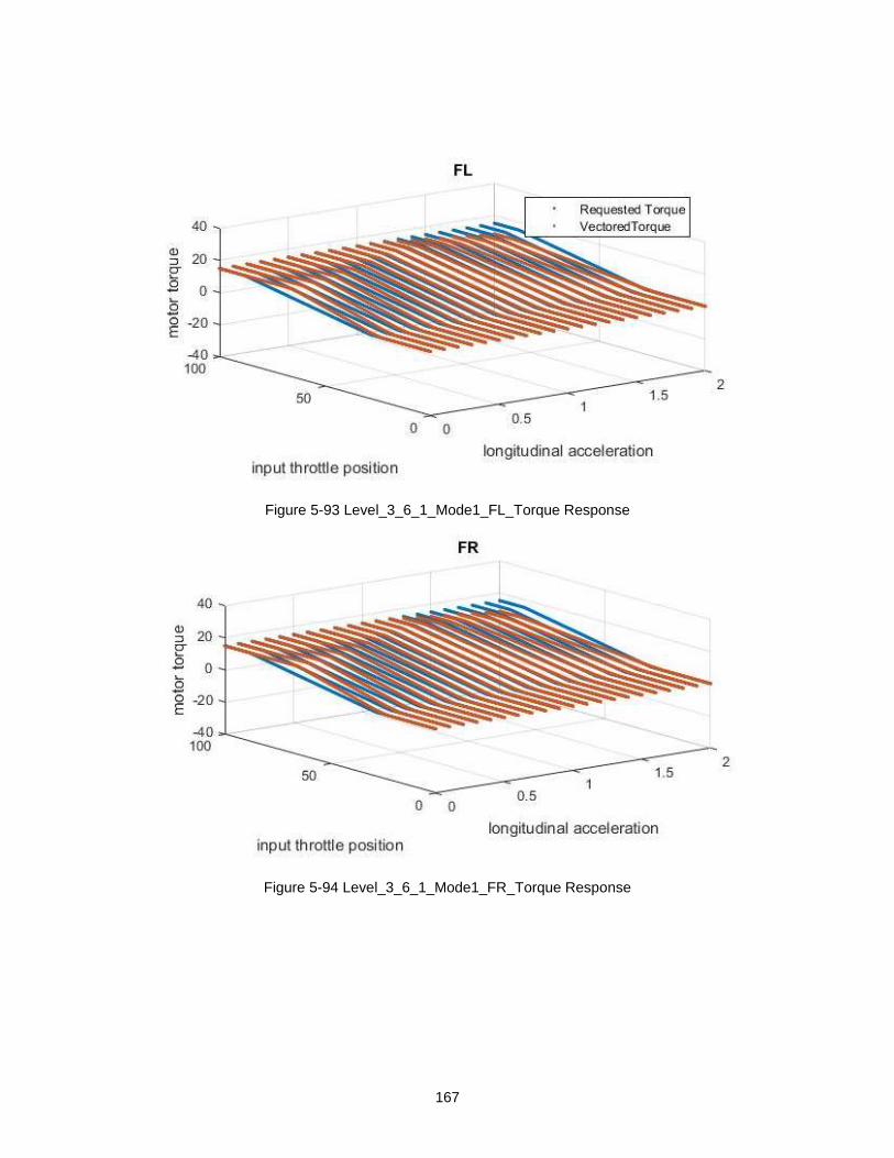
167
Figure 5-93 Level_3_6_1_Mode1_FL_Torque Response
Figure 5-94 Level_3_6_1_Mode1_FR_Torque Response

168
Figure 5-95 Level_3_6_1_Mode1_RL_Torque Response
Figure 5-96 Level_3_6_1_Mode1_RR_Torque Response

169
Level_3_7 and Level_3_8
Level_ 3_7 and Level_ 3_8 testing set up are testing torque vectoring controller program
response to lateral acceleration. In level _3_7 the car lateral acceleration varies from -
2g’s to 0g’s(left hand turn) and the lateral acceleration varies from 0-2 ( right hand
turn).The controller program has tested for mode 1 and mode 2.
Level 3_7 Testing
The car is taking left hand turn, means more weight would transfer to more right hand
side wheels. . The torque applied on right hand side wheel should be greater than left
hand side wheels.
The response of torque vectoring controller program during mode 1 should produce more
torque on front right wheels and vectored torque applied on right hand side should increase
with increase in lateral acceleration.
In mode 2, torque-vectoring controller would apply more torque on right hand side wheels
.However, the vectored torque applied on rear right wheels would be more than front right
wheels. The amount of toque put on right wheels should increase with increase in lateral
acceleration. The responses of controller in mode 1 and mode 2 are as follows

170
Figure 5-97 Level_3_7_Mode1_FL_Torque Response
Figure 5-98 Level_3_7_Mode1_FR_Torque Response
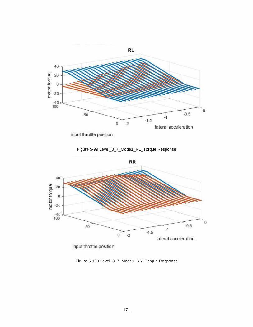
171
Figure 5-99 Level_3_7_Mode1_RL_Torque Response
Figure 5-100 Level_3_7_Mode1_RR_Torque Response

172
Figure 5-101 Level_3_7_Mode2_FL_Torque Response
Figure 5-102 Level_3_7_Mode2_FR_Torque Response

173
Figure 5-103 Level_3_7_Mode2_RL_Torque Response
Figure 5-104 Level_3_7_Mode2_RR_Torque Response

174
Level 3_8 Testing
The car is taking right hand turn, means more weight would transfer to more left hand
side wheels. The vectored torque on left hand side wheels should be greater than right
hand side wheels.
The response of torque vectoring controller program during mode 1 should produce more
torque on front left wheel and vectored torque applied on left hand side should increase
with increase in lateral acceleration.
In mode 2, torque-vectoring controller would apply more torque on left hand side wheels
.However, the vectored torque applied on rear left wheels would be more than front left
wheels. The amount of toque put on left wheels would increase with increase in lateral
acceleration. The responses of controller in mode 1 and mode 2 are as follows

175
Figure 5-105 Level_3_8_Mode1_FL_Torque Response
Figure 5-106 Level_3_8_Mode1_FR_Torque Response

176
Figure 5-107 Level_3_8_Mode1_RL_Torque Response
Figure 5-108 Level_3_8_Mode1_RR_Torque Response

177
Figure 5-109 Level_3_8_Mode2_FL_Torque Response
Figure 5-110 Level_3_8_Mode2_FR_Torque Response

178
Figure 5-111 Level_3_8_Mode2_RL_Torque Response
Figure 5-112 Level_3_8_Mode2_RR_Torque Response

179
Chapter 6
Conclusion and Future Work
Conclusions
The main aim of this thesis study was to developed model based active torque
vectoring controller in order distribute torque across four wheels to maximizes use of use
of all tires. The second goal of this thesis study was to developed linear predictive controller
response without any driver intervention; to obtain predictive torque vectoring controller
that would able to produce predictive response in different driving conditions and increase
the performance of car. The controller algorithm design presented in Chapter 4. The testing
controller responses to different driving maneuvers in chapter 5, these goals can be
concluded.
This testing (simulations) of controller is carried out in MATLAB-SIMULINK with
the help of testing program, which would able to reproduce different driving maneuvers.
The response of driver throttle and regen brake inputs are interpreted through linear motor
models presented in Chapter 2. These linear models would able to produce linear response
for driver in all driving conditions. The vehicle dynamics model used for development of
this controller is presented in Chapter 3. The design of controller based on steady state
vehicle dynamics equation give controller to work in different driving conditions and
maneuvers. For example, if car produces same lateral acceleration, longitudinal
acceleration or combination of both in different driving conditions (Ex: wet track and dry
track) controller would respond similarly to these situations. The input required for these
models can be easily obtained with simple sensor network on car. The additional safety
major has taken in case of accelerometer failure happens. The controller has designed
based on driver steering wheel input.

180
The torque-vectoring controller has designed based on two philosophies. As it can
see simulations, the torque-vectoring controller would not able to distribute driver
requested torque due to torque limit of motor. This happens due to mismatch of weight
distribution and power. The car is front heavy while more power is installed on rear wheels.
It has observed that during cornering front outside wheels get more weight than rear
outside wheel due to limitation to suspension design and in some cases, the front outside
motor supposed to put more torque than motor capacity. In this scenario, torque-vectoring
controller applies less torque on wheels than driver requested torque. The two differential
strategy is included for maximizing driver requested torque. The tire study shows that, this
strategy should work in normal competition setting. However, it can be only confirmed from
physical testing of car. These two strategies are explained throughout the chapter 4. In
theory, it is possible to extract 90% of performance of car with this controller design.
The tire modelling and tire data was not part of this study. The basic idea while
development of this controller was to developed simple torque vectoring controller, on
which further improvement in controller design can be made. The plan regarding further
development of torque vectoring controller has discussed in future work section
This controller design can be used for design of torque vectoring controller based on
transient vehicle dynamics model and active yaw controller. The further step would be
inclusion of tire model along with yaw control controller.
For dynamic response of controller have been torque vectoring controller, the
simulations has been performed on vehicle dynamics software IPG carmaker for FSAE
skid pad. The results obtain from this skid pad has shown expected response of controller.
It was hard to produce regenerative braking system design within IPG carmaker due to
time constrained, these results are not part of this thesis report.

181
Future Work
The scope of torque vectoring controller can be expanded into several aspect to
increase the performance of car. However as this was a first torque vectoring controller
for UTA racing emphasis has given on functional requirements rather than extracting 100%
performance of car. Future work will be of importance to increase performance of car.
The detailed transient vehicle dynamics model, which includes Yaw, pitch roll
velocity and acceleration. The normal load calculations based on transient model
would reduce the error involved with steady state calculation and increase the
performance of car
The active yaw control controller merged with these transient vehicle dynamics
model would give ability to control car around corner to maximize performance
The scaled tire model obtained from tire testing data and merged with any of above
controller, can be used to determine traction limit of tire during longitudinal or
lateral acceleration or combination of both and performance of car would increase.
If inverse transient model coupled with neural network can be installed on car, so
that car would able determine coefficient of friction between track and tire. Car
needs to install higher computing power to facilitate neural network installation.

182
Appendix A
Motors Data

183
Front and Rear- Torque Speed Data Points
Rear motor
Front motor
Speed Peak Torque Speed Peak Torque
RPM N.m RPM N.m
0 29.46951563 0 14.93532619
164.8351648 29.46577387 164.8351648 14.93275991
329.6703297 29.46203211 329.6703297 14.93009431
494.5054945 29.45829035 494.5054945 14.92732933
659.3406593 29.45454859 659.3406593 14.92446494
824.1758242 29.45080683 824.1758242 14.92150108
989.010989 29.44706508 989.010989 14.91843771
1153.846154 29.44332332 1153.846154 14.91527476
1318.681319 29.43958156 1318.681319 14.91201217
1483.516484 29.4358398 1483.516484 14.90864986
1648.351648 29.43209804 1648.351648 14.90518778
1813.186813 29.42835629 1813.186813 14.90162584
1978.021978 29.42461453 1978.021978 14.89796395
2142.857143 29.42087277 2142.857143 14.89420203
2307.692308 29.41713101 2307.692308 14.89033999
2472.527473 29.41338925 2472.527473 14.88637772
2637.362637 29.40964749 2637.362637 14.88231513
2802.197802 29.40590574 2802.197802 14.8781521
2967.032967 29.40216398 2967.032967 14.87388853
3131.868132 29.39842222 3131.868132 14.86952429
3296.703297 29.39468046 3296.703297 14.86505926
3461.538462 29.3909387 3461.538462 14.86049331
3626.373626 29.38719694 3626.373626 14.85582632
3791.208791 29.38345519 3791.208791 14.85105813
3956.043956 29.37971343 3956.043956 14.84618861
4120.879121 29.37597167 4120.879121 14.84121762
4285.714286 29.37222991 4285.714286 14.83614498
4450.549451 29.36848815 4450.549451 14.83097055
4615.384615 29.36474639 4615.384615 14.82569417
4780.21978 29.36100464 4780.21978 14.82031565
4945.054945 29.35726288 4945.054945 14.81483484
5109.89011 29.35352112 5109.89011 14.80925154
5274.725275 29.34977936 5274.725275 14.80356558
5439.56044 29.3460376 5439.56044 14.79777676
5604.395604 29.34229585 5604.395604 14.79188488
5769.230769 29.33855409 5769.230769 14.78588976
5934.065934 29.33481233 5934.065934 14.77979117
098.901099 29.33107057 6098.901099 14.77358891
6263.736264 29.32732881 6263.736264 14.76728276
6428.571429 29.32358705 6428.571429 14.74557704
6593.406593 29.3198453 6593.406593 14.68843735
Rear Motors Front Motors

184
Speed Peak Torque Speed Peak Torque
RPM N.m RPM N.m
6758.241758 29.30962971 6758.241758 14.60323128
6923.076923 29.24045689 6923.076923 14.49715062
7087.912088 29.11299589 7087.912088 14.37681494
7252.747253 28.94146005 7252.747253 14.23511216
7417.582418 28.73896667 7417.582418 14.08731291
7582.417582 28.5174911 7582.417582 13.93881199
7747.252747 28.26100233 7747.252747 13.77645245
7912.087912 28.00010559 7912.087912 13.6198587
8076.923077 27.71135083 8076.923077 13.45257265
8241.758242 27.43110396 8241.758242 13.27473453
8406.593407 27.12928327 8406.593407 13.10969863
8571.428571 26.80612121 8571.428571 12.93679662
8736.263736 26.50557549 8736.263736 12.7813945
8901.098901 26.18905793 8901.098901 12.59418136
9065.934066 25.90465164 9065.934066 12.45377577
9230.769231 25.55897464 9230.769231 12.28171693
9395.604396 25.24986974 9395.604396 12.09907354
9560.43956 24.98310469 9560.43956 11.85185029
9725.274725 24.65359003 9725.274725 11.52977578
9890.10989 24.37001375 9890.10989 11.29287942
10054.94505 24.07893091 10054.94505 10.98435605
10219.78022 23.78042903 10219.78022 10.75744099
10384.61538 23.4745979 10384.61538 10.46196244
10549.45055 23.16152954 10549.45055 10.24462268
10714.28571 22.90517894 10714.28571 9.962318428
10879.12088 22.57932247 10879.12088 9.688430025
11043.95604 22.31286725 11043.95604 9.422508515
11208.79121 22.04200372 11208.79121 9.227569534
11373.62637 21.76678396 11373.62637 8.974578069
11538.46154 21.33871727 11538.46154 8.72844431
11703.2967 20.91892411 11703.2967 8.488813294
11868.13187 20.50515931 11868.13187 8.198382279
12032.96703 20.09733633 12032.96703 7.972198402
12197.8022 19.69536407 12197.8022 7.751510216
12362.63736 19.29914768 12362.63736 7.536046967
12527.47253 18.90858929 12527.47253 7.274146473
12692.30769 18.39771982 12692.30769 7.019547471
12857.14286 18.01997049 12857.14286 6.82045939
13021.97802 17.64753871 13021.97802 6.577932883
13186.81319 17.28031989 13186.81319 6.341569771
13351.64835 16.80037094 13351.64835 6.111014405
13516.48352 16.4461586 13516.48352 5.885934204
13681.31868 15.98367684 13681.31868 5.623002157
13846.15385 15.64204681 13846.15385 5.367004969
14010.98901 15.19566162 14010.98901 5.117476895
Front Motors Rear Motors

185
Speed Peak Torque Speed Peak Torque
RPM N.m RPM N.m
14175.82418 14.86561657 14175.82418 4.873984764
14340.65934 14.43405899 14340.65934 4.59731406
14505.49451 14.11469018 14505.49451 4.327714819
14670.32967 13.69680227 14670.32967 4.027821693
14835.16484 13.28624403 14835.16484 3.735684135
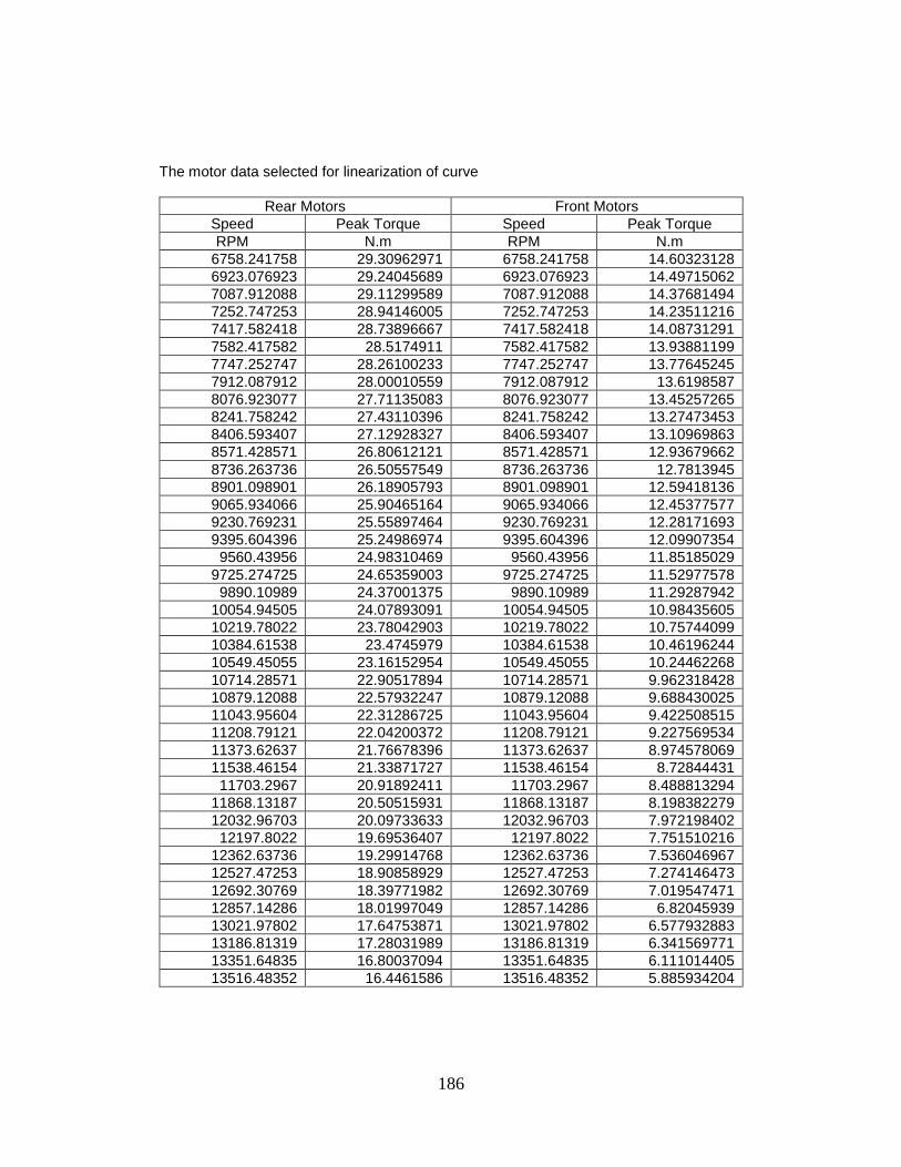
186
The motor data selected for linearization of curve
Rear Motors Front Motors
Speed Peak Torque Speed Peak Torque
RPM N.m RPM N.m
6758.241758 29.30962971 6758.241758 14.60323128
6923.076923 29.24045689 6923.076923 14.49715062
7087.912088 29.11299589 7087.912088 14.37681494
7252.747253 28.94146005 7252.747253 14.23511216
7417.582418 28.73896667 7417.582418 14.08731291
7582.417582 28.5174911 7582.417582 13.93881199
7747.252747 28.26100233 7747.252747 13.77645245
7912.087912 28.00010559 7912.087912 13.6198587
8076.923077 27.71135083 8076.923077 13.45257265
8241.758242 27.43110396 8241.758242 13.27473453
8406.593407 27.12928327 8406.593407 13.10969863
8571.428571 26.80612121 8571.428571 12.93679662
8736.263736 26.50557549 8736.263736 12.7813945
8901.098901 26.18905793 8901.098901 12.59418136
9065.934066 25.90465164 9065.934066 12.45377577
9230.769231 25.55897464 9230.769231 12.28171693
9395.604396 25.24986974 9395.604396 12.09907354
9560.43956 24.98310469 9560.43956 11.85185029
9725.274725 24.65359003 9725.274725 11.52977578
9890.10989 24.37001375 9890.10989 11.29287942
10054.94505 24.07893091 10054.94505 10.98435605
10219.78022 23.78042903 10219.78022 10.75744099
10384.61538 23.4745979 10384.61538 10.46196244
10549.45055 23.16152954 10549.45055 10.24462268
10714.28571 22.90517894 10714.28571 9.962318428
10879.12088 22.57932247 10879.12088 9.688430025
11043.95604 22.31286725 11043.95604 9.422508515
11208.79121 22.04200372 11208.79121 9.227569534
11373.62637 21.76678396 11373.62637 8.974578069
11538.46154 21.33871727 11538.46154 8.72844431
11703.2967 20.91892411 11703.2967 8.488813294
11868.13187 20.50515931 11868.13187 8.198382279
12032.96703 20.09733633 12032.96703 7.972198402
12197.8022 19.69536407 12197.8022 7.751510216
12362.63736 19.29914768 12362.63736 7.536046967
12527.47253 18.90858929 12527.47253 7.274146473
12692.30769 18.39771982 12692.30769 7.019547471
12857.14286 18.01997049 12857.14286 6.82045939
13021.97802 17.64753871 13021.97802 6.577932883
13186.81319 17.28031989 13186.81319 6.341569771
13351.64835 16.80037094 13351.64835 6.111014405
13516.48352 16.4461586 13516.48352 5.885934204

187
Rear Motors Front Motors
Speed Peak Torque Speed Peak Torque
RPM N.m RPM N.m
13846.15385 15.64204681 13846.15385 5.367004969
13681.31868 15.98367684 13681.31868 5.623002157
14010.98901 15.19566162 14010.98901 5.117476895
14175.82418 14.86561657 14175.82418 4.873984764
14340.65934 14.43405899 14340.65934 4.59731406
14505.49451 14.11469018 14505.49451 4.327714819
14670.32967 13.69680227 14670.32967 4.027821693
14835.16484 13.28624403 14835.16484 3.735684135

188
Appendix B Motor
Controller Programs

189
Front100TScurveGenerator
% copy given torque values in TF matrix
% copy corresponding speed values in TFS matrix
plot(TFS,TF,'r','linewidth',3)
axis([0 15000 0 15])
set(gca,'fontsize',18)
grid on
grid minor
xlabel('\bfSpeed (rpm)');
ylabel('\bf Torque (N-m)')
legend('\bf Front Motor-100% Throttle characteristic');
title('\bfE-16 Torque Vs Speed Graph-Front Motors 100% Throttle Characteristics');

190
FrontTScurveGenerator
S_peakf=17674.91; % from Curve Fit rear Motor_Torque speed Curve Fit_LAR
T_peakf=25.01; % From Curve Fit Re Motor_Torque speed Curve Fit_LAR
T_maxf_100=15;
Res=zeros();
n=0;
for TP=1:5:100
tp=(TP/100);
S_max= tp*S_peakf;
T_max=tp*T_peakf;
for S=0:1:S_max
n=n+1;
throttle_position=(TP/100); % Converting Throttle Position from Percentage to absolute
S_maxf= throttle_position*S_peakf;
T_maxf=throttle_position*T_peakf;
if S<S_maxf
Tf=-(T_peakf/S_peakf)*S+(T_maxf);
if Tf>T_maxf_100 % If Calacualted Torque of Rear Left Motor is greater than Max
Output Torque
Tf=T_maxf_100;% if yes then calculated Torque is T_maxf_100
end
else
Tf=0;

191
end
Res(n,1)=Tf;
Res(n,2)=S;
end
plot(Res(:,2),Res(:,1),'r--','linewidth',2);
hold on
Res=0;
end
axis([0 15000 0 15])
set(gca,'fontsize',18)
grid on
grid minor
xlabel('\bfSpeed (rpm)');
ylabel('\bf Torque (N-m)')
legend('\bf Front Motor 5% increment throttle characteristic');
title('\bfE-16 Torque Vs Speed Graph-Front Motor Throttle Characteristics');
hold on

192
Rear100TScurveGenerator.
% copy given torque values in TR matrix
% copy corresponding speed values in TRS matrix
set(gca,'fontsize',18)
plot(TRS,TR,'k','linewidth',2);
set(gca,'fontsize',18)
axis([0 15000 0 30])
grid on
grid minor
xlabel('\bfspeed (rpm)');
ylabel('\bf Torque (N-m)')
legend('\bf Rear Motor-100% Throttle Charateristics');
title('\bfE-16 Torque Vs Speed Graph-Rear Motor 100% Throttle characteristics');
hold on

193
RearTScurveGenerator.m
S_peakr=21715; % from Curve Fit rear Motor_Torque speed Curve Fit_LAR
T_peakr=44.21; % From Curve Fit Re Motor_Torque speed Curve Fit_LAR
T_maxr_100=30;
Res=zeros();
n=0;
for TP=1:5:100
tp=(TP/100);
S_max= tp*S_peakr;
T_max=tp*T_peakr;
for S=0:1:S_max
n=n+1;
throttle_position=(TP/100); % Converting Throttle Position from Percentage to absolute
S_maxr= throttle_position*S_peakr;
T_maxr=throttle_position*T_peakr;
if S<S_maxr
Tf=-(T_peakr/S_peakr)*S+(T_maxr);
if Tf>T_maxr_100 % If Calacualted Torque of Rear Left Motor is greater than Max
Output Torque
Tf=T_maxr_100;% if yes then calculated Torque is T_maxf_100
end
else
Tf=0;

194
end
Res(n,1)=Tf;
Res(n,2)=S;
end
plot(Res(:,2),Res(:,1),'k--','linewidth',2);
hold on
Res=0;
end
axis([0 15000 0 30])
set(gca,'fontsize',18)
grid on
grid minor
xlabel('\bfSpeed (rpm)');
ylabel('\bf Torque (N-m)')
legend('\bf Rear Motor 5% increment throttle characteristic');
title('\bfE-16 Torque Vs Speed Graph-Rear Throttle Characteristics');

195
FrontTScurveGeneratorRev.m
S_peakf=17674.91; % from Curve Fit rear Motor_Torque speed Curve Fit_LAR
T_peakf=-25.01; % From Curve Fit Re Motor_Torque speed Curve Fit_LAR
T_maxf_100=-15;
Res=zeros();
n=0;
for RP=1:5:100
tp=(RP/100);
S_max= tp*S_peakf;
T_max=tp*T_peakf;
for S=0:1:S_max
n=n+1;
regen_position=(RP/100); % Converting Throttle Position from Percentage to absolute
S_maxf= regen_position*S_peakf;
T_maxf=regen_position*T_peakf;
if S<S_maxf
TR=(-T_peakf/S_peakf)*S+(T_maxf);
if TR<T_maxf_100 % If Calacualted Torque of Rear Left Motor is greater than Max
Output Torque
TR=T_maxf_100;% if yes then calculated Torque is T_maxf_100
end
else
TR=0;
end

196
Res(n,1)=TR;
Res(n,2)=S;
end
plot(Res(:,2),Res(:,1),'r--','linewidth',2);
hold on
Res=0;
end
axis([0 15000 -15 0])
set(gca,'fontsize',18)
grid on
grid minor
xlabel('\bfSpeed (rpm)');
ylabel('\bf Torque (N-m)')
legend('\bf Front Motor 5% increment regenrative characteristic');
title('\bfE-16 Torque Vs Speed Graph-Front Motor Regenrative Characteristics');
hold on
RearTScurveGeneratorRev
S_peakr=21715; % from Curve Fit rear Motor_Torque speed Curve Fit_LAR
T_peakr=-44.21; % From Curve Fit Re Motor_Torque speed Curve Fit_LAR
T_maxr_100=-30;
Res=zeros();
n=0;
for RP=1:5:100

197
tp=(RP/100);
S_max= tp*S_peakr;
T_max=tp*T_peakr;
for S=0:1:S_max
n=n+1;
regen_position=(RP/100); % Converting Throttle Position from Percentage to absolute
S_maxr= regen_position*S_peakr;
T_maxr=regen_position*T_peakr;
if S<S_maxr
TR=(-T_peakr/S_peakr)*S+(T_maxr);
if TR<T_maxr_100 % If Calacualted Torque of Rear Left Motor is greater than Max
Output Torque
TR=T_maxr_100;% if yes then calculated Torque is T_maxf_100
end
else
TR=0;
end
Res(n,1)=TR;
Res(n,2)=S;
end
plot(Res(:,2),Res(:,1),'k--','linewidth',2);

198
Appendix C
Torque Vectoring Controller Program

199
Ediff.m
function
[lambda_TV_FL_Regen,lambda_TV_FR_Regen,lambda_TV_RL_Regen,lambda_TV_RR_Regen,lambda
_TV_FL_Throttle, lambda_TV_FR_Throttle, lambda_TV_RL_Throttle,
lambda_TV_RR_Throttle]=E_diff(torque_mode_selection, throttle_position, regen_brake_position,
steering_wheel_angle,accel_lat,accel_long, front_left_motor_rpm, front_right_motor_rpm,
rear_left_motor_rpm, rear_right_motor_rpm)
%% Suspension Parameters
mass_of_car= 326.58 ; % Mass of Car with Driver in Kgs
% front_weight_distribution=55; % Front Weight Distribution
front_unsprung_mass=48; % front Unsprung Mass at Front Unsprung Mass CG
rear_unsprung_mass=50; % Rear Unsprung Mass at Rear Sprung Mas CG
sprung_mass_car=228.61; % Sprung Mass of Car in Kg
distance_front_unsprung_cg=260.35/1000;% Front Unsprung Mass CG in mm- Input in MM-Getting
Converted into M for all below values
distance_rear_unsprung_cg=260.35/1000; % Rear Unsprungit g Mass CG in mm- Input in MM
distance_of_sprung_cg_from_front_axle=760/1000; % Distance of Sprung CG from Front Axle in mm
wheel_base=1676.4/1000; % Wheel base in MM
distance_of_sprung_cg_from_rear_axle=wheel_base-distance_of_sprung_cg_from_front_axle;
distance_sprung_mass_cg_and_roll_axis=228.611/1000; % Perpendicular Distance Between Sprung
Mass CG and Roll Axis
cg_height= 292.1/1000; %CG Height in MM
distance_of_cg_from_front_axle=778.9164/1000; % X-Distance of CG from front Wheel Center
distance_of_cg_from_rear_axle=wheel_base-distance_of_cg_from_front_axle; % X-Distance of CG from
rear Wheel Center
g=9.81; % Acceleration Due to Gravity
front_roll_center_height=81.026/1000; % Front Roll Center Height

200
rear_roll_center_height=86.106/1000; % Rear Roll Center Height;
front_roll_rate=16016; % Front Roll Rate - From Excel Sheet- Will Write Program for it in Future
rear_roll_rate=19253.07;% Rear Roll Rate- N-m/rad-From Excel Sheet- Will Write Program for it in Future
modified_front_roll_rate=front_roll_rate-
(((distance_of_sprung_cg_from_rear_axle)*sprung_mass_car*g*distance_sprung_mass_cg_and_roll_axi
s)/wheel_base); % Kf' formula from RCVD Page 681
modified_rear_roll_rate=(rear_roll_rate-
((distance_of_sprung_cg_from_front_axle*sprung_mass_car*g*distance_sprung_mass_cg_and_roll_axis
)/(wheel_base))); % Kr' Formula from RCVD Pages 681
%% Steering Parameters
steering_wheel_compliance= 0.4 ; % Steering wheel play in steering
steering_ratio=3.31;
steeringangle_Play=(steering_wheel_compliance/steering_ratio)*(pi/180);
%% Aero parameters
drag_coefficient=0;
center_pressure_height=100/1000;
%% Drivetrain parameters
%Front Motors
S_peakf=17674.91; % from Curve Fit Front Motor_Torque speed Curve Fit_LAR
T_peakf=25.01; % From Curve Fit Front Motor_Torque speed Curve Fit_LAR
T_maxf_100=15; % From Motor Simulation Data
S_maxf_100=15000; %Per manufacturer

201
slope_front=-(T_peakf/S_peakf);
% Rear Motors
S_peakr=21715; % from Curve Fit rear Motor_Torque speed Curve Fit_LAR
T_peakr=44.21; % From Curve Fit Re Motor_Torque speed Curve Fit_LAR
T_maxr_100=30; % From Motor Simulation Data
S_maxr_100=15000; %Per manufacturer
slope_rear=-(T_peakr/S_peakr);
% Gears
gear_ratio=1/13;
% Wheels and Tires
wheel_diameter= 514.604/1000; %Diameter of Wheel
front_tread=1244.6/1000; % Front Tread in MM
rear_tread=1193.8/1000; % Rear Tread in MM
%% end of vehicle parameters %%
%..........................................................................
%..........................................................................
%% Manipulate Inputs for use in algorithm
%convert steering angle from deg to rad.
steering_angle_rad=(steering_wheel_angle/steering_ratio)*(pi/180); % steering wheel angle in radians
% Calculate Wheel Speed from Motor Speed
wheel_speed_rf = front_right_motor_rpm* gear_ratio; % Converting motor speed into wheel speed
wheel_speed_lf = front_left_motor_rpm * gear_ratio; % Convrting motor speed into wheel speed

202
wheel_speed_rr = rear_right_motor_rpm * gear_ratio; % Converting motor speed into wheel speed
wheel_speed_lr = rear_left_motor_rpm * gear_ratio; % Converting motor speed into wheel speed
% Calculaton of Linear Velcoity
linear_velocity_rf=pi*wheel_diameter*(wheel_speed_rf/60); % Linear velocity of front right wheel in m/s
linear_velocity_lf=pi*wheel_diameter*(wheel_speed_lf/60); %Linear velocity of front left wheel in m/s
linear_velocity_lr=pi*wheel_diameter*(wheel_speed_rr/60); % Linear Velocity of rear left wheel in m/s
linear_velocity_rr=pi*wheel_diameter*(wheel_speed_lr/60); % Linear Velocity of reaar right wheel in m/s
average_velocity_car=(linear_velocity_rf+linear_velocity_lf+linear_velocity_lr+linear_velocity_rr)/4;
if average_velocity_car<1.38889 %5 kph in m/s
regen_brake_position=0;
end
%--will get vehicle velocity from Randy so
% can delete these lines and make average_velocity_car a direct input.
%% Input Modification - Solving lost or delayed Lateral Acceleration input problem
% Here we are managing if Driver want to steer and we are not reciving
% Lateral acceleration input from acclerometer then average the Velocity
% of vehicle and then Calculate Raduis of turn at CG and a_lat= V^2/R
%REMEMBER THIS IS ONLY FOR INITIAL FEW MILISECONDS TO HELP DRIVER TO TAKE TURN
%Side Note -We can Reduce this loop during program Optimization if we dont
%want to Calculate or record values of Velocity
% Estimate of Radius of Turn of Center to Calculate Lateral Acceleration
if steering_angle_rad < -steeringangle_Play && accel_lat==0 % Left hand Turn lateral accelration input
==0
turn_radius_lr= wheel_base/tan(abs(steering_angle_rad)); %dist from LR wheel to turn center in m.
turn_radius_rr= front_tread+turn_radius_lr; %dist from RR wheel to turn center in m.

203
turn_radius_rf= sqrt((turn_radius_lr^2)+(wheel_base^2)); %dist from RF wheel to turn center in m.
turn_radius_lf= sqrt((turn_radius_rr^2)+(wheel_base^2)); %dist from LF wheel to turn center in m.
turn_radius_CG=sqrt(((turn_radius_lr+front_tread*0.5)^2)+(distance_of_cg_from_rear_axle^2)); %
Radius of Turn
accel_lat=-(average_velocity_car^2)/(turn_radius_CG*g) % Averaged Lateral G for car
%accel_lat=accel_lat1;
end
if steering_angle_rad >= steeringangle_Play && accel_lat==0 % Right hand Turn lateral accelration input
==0
turn_radius_rr= wheel_base/tan(abs(steering_angle_rad)); %dist from RR wheel to turn center in m.
turn_radius_lr= front_tread+turn_radius_rr; %dist from LR wheel to turn center in m.
turn_radius_rf= sqrt((turn_radius_rr^2)+(wheel_base^2)); %dist from RF wheel to turn center in m.
turn_radius_lf= sqrt((turn_radius_lr^2)+(wheel_base^2)); %dist from LF wheel to turn center in m.
turn_radius_CG=sqrt(((turn_radius_rr+front_tread*0.5)^2)+(distance_of_cg_from_rear_axle^2));
accel_lat=(average_velocity_car^2)/(turn_radius_CG*g); % Averaged Lateral G for car
% accel_lat=accel_lat1;
end
%% Calculation of Longitudinal Load Transfer
front_single_wheel_normal_load=(mass_of_car*distance_of_cg_from_rear_axle -
drag_coefficient*center_pressure_height-mass_of_car*accel_long*cg_height)/(2*wheel_base); % Weight
Transfer equation for Front Individual tires during longitudinal acceleration
rear_single_wheel_normal_load
=(mass_of_car*distance_of_cg_from_front_axle+drag_coefficient*center_pressure_height+mass_of_car*
accel_long*cg_height)/(2*wheel_base); % Weight Transfer equation for Rear Individual tires during
longitudinal acceleration

204
%% Calculation of Lateral Load Transfer-RCVD-Milleken Formulas
front_normal_lateral_load_transfer=accel_lat*(((sprung_mass_car*g/front_tread)*((((distance_sprung_ma
ss_cg_and_roll_axis*modified_front_roll_rate)/(front_roll_rate+rear_roll_rate-
sprung_mass_car*g*distance_sprung_mass_cg_and_roll_axis))+(((distance_of_sprung_cg_from_rear_ax
le)/wheel_base)*front_roll_center_height))))+((front_unsprung_mass*g*distance_front_unsprung_cg)/(fro
nt_tread)));%RCVD PAge 682 Formula Force in N
front_normal_lateral_load_transfer=front_normal_lateral_load_transfer/g; % Convering it to Kg
rear_normal_lateral_load_transfer
=accel_lat*(((sprung_mass_car*g/rear_tread)*((((distance_sprung_mass_cg_and_roll_axis*modified_rear
_roll_rate)/(front_roll_rate+rear_roll_rate-
sprung_mass_car*g*distance_sprung_mass_cg_and_roll_axis))+(((distance_of_sprung_cg_from_front_a
xle)/wheel_base)*rear_roll_center_height))))+((rear_unsprung_mass*g*distance_rear_unsprung_cg)/(rear
_tread))); %RCVD Page 682 Fromula Force in N
rear_normal_lateral_load_transfer =rear_normal_lateral_load_transfer/g; % Converting it to Kg
%% Calculation of Individual Wheel Load
% For Right Turn Scenario
normal_load_lf=front_single_wheel_normal_load+front_normal_lateral_load_transfer;
normal_load_rf=front_single_wheel_normal_load-front_normal_lateral_load_transfer;
normal_load_lr=rear_single_wheel_normal_load+rear_normal_lateral_load_transfer;
normal_load_rr=rear_single_wheel_normal_load-rear_normal_lateral_load_transfer;
% end
%% Calculation of Motor Torques During Regenrative Breaking
if regen_brake_position>0

205
regen_brake_position=(regen_brake_position/100); % Converting Throttle Position from Percentage to
absolute
%% Calculation of Brake Torque for Front Motors
S_maxf=regen_brake_position*S_peakf; % Calculating S-axis intercept for given Throttle Position
T_maxf=regen_brake_position*-T_peakf; % Calculating T axis intercept for given Throttle Position
if front_left_motor_rpm< S_maxf
requested_torque_front_left_motor=-(slope_front)*front_left_motor_rpm+(T_maxf); %%%%%%
Calculating Torque at given Speed %Vhange calculaton defined it once only
if requested_torque_front_left_motor<-T_maxf_100 % if front left calculated torque greater than
Maximum capacity
requested_torque_front_left_motor=-T_maxf_100; % if yes then calculated Torque is T_maxf_100
elseif requested_torque_front_left_motor >0
requested_torque_front_left_motor=0;
end
else
requested_torque_front_left_motor=0;
end
if front_right_motor_rpm < S_maxf
requested_torque_front_right_motor=-(slope_front)*front_right_motor_rpm+(T_maxf);
if requested_torque_front_right_motor<-T_maxf_100 % if front right calculated torque greater than
Maximum capacity
requested_torque_front_right_motor=-T_maxf_100;% if yes then calculated Torque is
T_maxf_100
elseif requested_torque_front_right_motor >0
requested_torque_front_right_motor=0;
end
else

206
requested_torque_front_right_motor=0;
end
%% Calculation of Brake Torque for Rear Motors
S_maxr=regen_brake_position*S_peakr;
T_maxr=regen_brake_position*-T_peakr;
if rear_left_motor_rpm<S_maxr
requested_torque_rear_left_motor=-(slope_rear)*rear_left_motor_rpm+(T_maxr);
if requested_torque_rear_left_motor<-T_maxr_100 % If Calacualted Torque of Rear Left Motor is
greater than Max Output Torque
requested_torque_rear_left_motor=-T_maxr_100;% if yes then calculated Torque is T_maxf_100
elseif requested_torque_rear_left_motor >0
requested_torque_rear_left_motor=0;
end
else
requested_torque_rear_left_motor=0;
end
if rear_right_motor_rpm<S_maxr
requested_torque_rear_right_motor=-(slope_rear)*rear_right_motor_rpm+(T_maxr);
if requested_torque_rear_right_motor<-T_maxr_100 % if front right calculated torque greater than
Maximum capacity
requested_torque_rear_right_motor=-T_maxr_100; % if yes then calculated Torque is
T_maxf_100
elseif requested_torque_rear_right_motor >0
requested_torque_rear_right_motor=0;
end
else

207
requested_torque_rear_right_motor=0;
end
if torque_mode_selection==1 % Mode Control
requested_total_torque=requested_torque_front_left_motor+requested_torque_front_right_motor+request
ed_torque_rear_left_motor+requested_torque_rear_right_motor; % Total absolute torue Avarege
torque_front_left_output=(normal_load_lf/mass_of_car)*requested_total_torque; % Output Front Left
Torque based on weight Ratio
% if torque_front_left_output<-T_maxf_100
% torque_front_left_output=-T_maxf_100;
% end
torque_front_right_output=(normal_load_rf/mass_of_car)*requested_total_torque; % Output-Front
Right Torque based in Weight Ratio
% if torque_front_right_output<-T_maxf_100
% torque_front_right_output=-T_maxf_100;
% end
torque_rear_left_output=(normal_load_lr/mass_of_car)*requested_total_torque; % Output-Rear Left
Torque Based on weight Ratio
% if torque_rear_left_output<-T_maxf_100
% torque_rear_left_output=-T_maxf_100;
% end
torque_rear_right_output=(normal_load_rr/mass_of_car)*requested_total_torque; % Output
% if torque_rear_right_output<-T_maxf_100
% torque_rear_right_output=-T_maxf_100;
% end
else % Mode Insane

208
requested_torque_front=requested_torque_front_left_motor+requested_torque_front_right_motor; %
Total absolute Torque Front
requested_torque_rear=requested_torque_rear_left_motor+requested_torque_rear_right_motor; %
Total absolute torue rear
requested_total_torque=requested_torque_front+requested_torque_rear;% For checking
torque_front_left_output=(normal_load_lf/(2*front_single_wheel_normal_load))*requested_torque_front;
% Output Front Left Torque based on weight Ratio
torque_front_right_output=(normal_load_rf/(2*front_single_wheel_normal_load))*requested_torque_front;
% Output-Front Right Torque based in Weight Ratio
torque_rear_left_output=(normal_load_lr/(2*rear_single_wheel_normal_load))*requested_torque_rear; %
Output-Rear Left Torque Based on weight Ratio
torque_rear_right_output=(normal_load_rr/(2*rear_single_wheel_normal_load))*requested_torque_rear;
% Output
end
%% Now once you calculate the required torque you need to check this torque does this torque greater
than 100 % torque at that throttle position
% Otherwise it will start giving us throttle position or regen brake
% position more than 100%
T_maxf_L_100=-(T_peakf/S_peakf)*front_left_motor_rpm+T_peakf; % Maximum possible torque
output from front left motor
if T_maxf_L_100>T_maxf_100
T_maxf_L_100=T_maxf_100;
end

209
T_maxf_R_100=-(T_peakf/S_peakf)*front_right_motor_rpm+T_peakf; % Maximum Possible torque
output from front right motor
if T_maxf_R_100>T_maxf_100
T_maxf_R_100=T_maxf_100;
end
T_maxr_L_100=-(T_peakr/S_peakr)*rear_left_motor_rpm+T_peakr;% Maximum possible torque output
from reaar left motor
if T_maxr_L_100>T_maxr_100
T_maxr_L_100=T_maxr_100;
end
T_maxr_R_100=-(T_peakr/S_peakr)*rear_right_motor_rpm+T_peakr; % Maximum possible torque
output from rear right motor
if T_maxr_R_100>T_maxr_100
T_maxr_R_100=T_maxr_100;
end
%if torque_front_left_output < 0
if torque_front_left_output<-T_maxf_L_100 % If required Reverse Torque is Less than 100 % Reverese
Capacity. Apply maximum revrse torque.
torque_front_left_output=-T_maxf_L_100; % Applying Maximum availaible Reverse Torque
end
%if torque_front_right_output < 0
if torque_front_right_output<-T_maxf_R_100 % If required Reverse Torque is Less than 100 %
Reverese Capacity. Apply maximum revrse torque.
torque_front_right_output=-T_maxf_R_100; % Applying Maximum availaible Reverse Torque
end
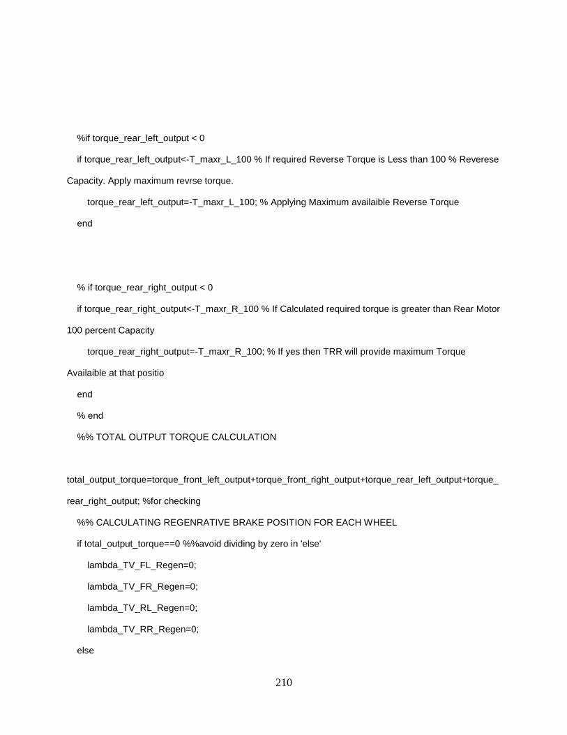
210
%if torque_rear_left_output < 0
if torque_rear_left_output<-T_maxr_L_100 % If required Reverse Torque is Less than 100 % Reverese
Capacity. Apply maximum revrse torque.
torque_rear_left_output=-T_maxr_L_100; % Applying Maximum availaible Reverse Torque
end
% if torque_rear_right_output < 0
if torque_rear_right_output<-T_maxr_R_100 % If Calculated required torque is greater than Rear Motor
100 percent Capacity
torque_rear_right_output=-T_maxr_R_100; % If yes then TRR will provide maximum Torque
Availaible at that positio
end
% end
%% TOTAL OUTPUT TORQUE CALCULATION
total_output_torque=torque_front_left_output+torque_front_right_output+torque_rear_left_output+torque_
rear_right_output; %for checking
%% CALCULATING REGENRATIVE BRAKE POSITION FOR EACH WHEEL
if total_output_torque==0 %%avoid dividing by zero in 'else'
lambda_TV_FL_Regen=0;
lambda_TV_FR_Regen=0;
lambda_TV_RL_Regen=0;
lambda_TV_RR_Regen=0;
else

211
lambda_TV_FL_Regen=((torque_front_left_output-(-(slope_front)*front_left_motor_rpm))/-
T_peakf)*100; %(1+t_fL_ratio)*itp; % New bp
lambda_TV_FR_Regen=((torque_front_right_output-(-(slope_front)*front_right_motor_rpm))/-
T_peakf)*100;%(1+t_fR_ratio)*itp; % New bP
lambda_TV_RL_Regen=((torque_rear_left_output-(-(slope_rear)*rear_left_motor_rpm))/-
T_peakr)*100;%(1+t_rL_ratio)*itp; % New BP
lambda_TV_RR_Regen=((torque_rear_right_output-(-(slope_rear)*rear_right_motor_rpm))/-
T_peakr)*100;%(1+t_rR_ratio)*itp; % New BP
end
lambda_TV_FL_Throttle=0;
lambda_TV_FR_Throttle=0;
lambda_TV_RL_Throttle=0;
lambda_TV_RR_Throttle=0;
else
throttle_position=(throttle_position/100); % Converting Throttle Position from Percentage to absolute
%% Calculation of Drive Torque Requested at Front Motors
S_maxf=throttle_position*S_peakf; % Calculating S-axis intercept for given Throttle Position- Redudant
T_maxf=throttle_position*T_peakf; % Calculating T axis intercept for given Throttle Position
if front_left_motor_rpm<S_maxf
requested_torque_front_left_motor=slope_front*front_left_motor_rpm+(T_maxf); % Calculating
Torque at given Speed
if requested_torque_front_left_motor>T_maxf_100 % if front left calculated torque greater than
Maximum capacity
requested_torque_front_left_motor=T_maxf_100; % if yes then calculated Torque is T_maxf_100
elseif requested_torque_front_left_motor<0
requested_torque_front_left_motor=0;
end

212
else
requested_torque_front_left_motor=0;
end
if front_right_motor_rpm<S_maxf
requested_torque_front_right_motor=slope_front*front_right_motor_rpm+(T_maxf);
if requested_torque_front_right_motor>T_maxf_100 % if front right calculated torque greater than
Maximum capacity
requested_torque_front_right_motor=T_maxf_100;% if yes then calculated Torque is T_maxf_100
% end
% if requested_torque_front_right_motor<-T_maxf_100 % if front right calculated torque greater
than Maximum capacity
% requested_torque_front_right_motor=-T_maxf_100;% if yes then calculated Torque is
T_maxf_100
elseif requested_torque_front_right_motor<0
requested_torque_front_right_motor=0;
end
else
requested_torque_front_right_motor=0;
end
%% Calculation of Drive Torque Requested at Rear Motors
S_maxr= throttle_position*S_peakr;
T_maxr=throttle_position*T_peakr;
requested_torque_rear_left_motor=slope_rear*rear_left_motor_rpm+(T_maxr);
if rear_left_motor_rpm<S_maxr

213
if requested_torque_rear_left_motor>T_maxr_100 % If Calacualted Torque of Rear Left Motor is
greater than Max Output Torque
requested_torque_rear_left_motor=T_maxr_100;% if yes then calculated Torque is T_maxf_100
elseif requested_torque_rear_left_motor<0
requested_torque_rear_left_motor=0;
end
else
requested_torque_rear_left_motor=0;
end
if rear_right_motor_rpm<S_maxr
requested_torque_rear_right_motor=slope_rear*rear_right_motor_rpm+(T_maxr);
if requested_torque_rear_right_motor>T_maxr_100 % if front right calculated torque greater than
Maximum capacity
requested_torque_rear_right_motor=T_maxr_100; % if yes then calculated Torque is T_maxf_100
elseif requested_torque_rear_right_motor<0
requested_torque_rear_right_motor=0;
end
else
requested_torque_rear_right_motor=0;
end
%% Distribution of Torque According to Weight Distribution and Mode
if torque_mode_selection==1 % Mode 1 Control

214
requested_total_torque=requested_torque_front_left_motor+requested_torque_front_right_motor+request
ed_torque_rear_left_motor+requested_torque_rear_right_motor; % Total absolute torue Avarege
torque_front_left_output=(normal_load_lf/mass_of_car)*requested_total_torque; % Output Front Left
Torque based on weight Ratio
% Taken care in bottom section
% if torque_front_left_output>T_maxf_100
% torque_front_left_output=T_maxf_100;
% end
torque_front_right_output=(normal_load_rf/mass_of_car)*requested_total_torque; % Output-Front
Right Torque based in Weight Ratio
% Taken care in bottom section
% if torque_front_right_output>T_maxf_100
% torque_front_right_output=T_maxf_100;
% end
torque_rear_left_output=(normal_load_lr/mass_of_car)*requested_total_torque; % Output-Rear Left
Torque Based on weight Ratio
% Taken care in bottom section
% if torque_rear_left_output>T_maxr_100
% torque_rear_left_output=T_maxr_100;
% end
torque_rear_right_output=(normal_load_rr/mass_of_car)*requested_total_torque; % Output- Rear
Right Torque Based in weight Ratio
% Taken care in bottom section
% if torque_rear_right_output>T_maxr_100
% torque_rear_right_output=T_maxr_100;
% end

215
else % Mode 2
requested_torque_front=requested_torque_front_left_motor+requested_torque_front_right_motor; %
Total absolute Torque Front
requested_torque_rear=requested_torque_rear_left_motor+requested_torque_rear_right_motor; %
Total absolute torue rear
requested_total_torque=requested_torque_front+requested_torque_rear;% For checking
torque_front_left_output=(normal_load_lf/(2*front_single_wheel_normal_load))*requested_torque_front;
% Output Front Left Torque based on weight Ratio
torque_front_right_output=(normal_load_rf/(2*front_single_wheel_normal_load))*requested_torque_front;
% Output-Front Right Torque based in Weight Ratio
torque_rear_left_output=(normal_load_lr/(2*rear_single_wheel_normal_load))*requested_torque_rear; %
Output-Rear Left Torque Based on weight Ratio
torque_rear_right_output=(normal_load_rr/(2*rear_single_wheel_normal_load))*requested_torque_rear;
% Output
end
%% Now once you calculate the required torque you need to check this torque does this torque greater
than 100 % torque at that throttle position
% Otherwise it will start giving us throttle position or regen brake
% position more than 100%
T_maxf_L_100=-(T_peakf/S_peakf)*front_left_motor_rpm+T_peakf; % Maximum possible torque
output from front left motor
if T_maxf_L_100>T_maxf_100
T_maxf_L_100=T_maxf_100;

216
end
T_maxf_R_100=-(T_peakf/S_peakf)*front_right_motor_rpm+T_peakf; % Maximum Possible torque
output from front right motor
if T_maxf_R_100>T_maxf_100
T_maxf_R_100=T_maxf_100;
end
T_maxr_L_100=-(T_peakr/S_peakr)*rear_left_motor_rpm+T_peakr;% Maximum possible torque output
from reaar left motor
if T_maxr_L_100>T_maxr_100
T_maxr_L_100=T_maxr_100;
end
T_maxr_R_100=-(T_peakr/S_peakr)*rear_right_motor_rpm+T_peakr; % Maximum possible torque
output from rear right motor
if T_maxr_R_100>T_maxr_100
T_maxr_R_100=T_maxr_100;
end
% Checking if the OUTPUT TORQUE IS GREATER THAN TORQUE AT 100 % THROTTLE
% POSITION
%if tp>0
% If calcualted Torque is Above Max Possible Output Capacity of Motor
if torque_front_left_output>T_maxf_L_100 % If Calculated required torque is greater than 100 percent
Motor Capacity
torque_front_left_output=T_maxf_L_100; % If yes then will provide maximum Torque Availaible at
Motor
end

217
if torque_front_left_output< -T_maxf_L_100 % If required Reverse Torque is Less than 100 %
Reverese Capacity. Apply maximum revrse torque.
torque_front_left_output=-T_maxf_L_100; % Applying Maximum availaible Reverse Torque
end
% If calcualted Torque is Above Max Possible Output Capacity of fornt Right Motor
if torque_front_right_output>T_maxf_R_100 % If Calculated required torque is greater than Front Motor
100 percent Capacity
torque_front_right_output=T_maxf_R_100; % We will provide MAximum Torque Avaialaible
end
% If calcualted Torque is Above Max Possible Output Capacity of Rear Left Motor
if torque_rear_left_output>T_maxr_L_100 % If Calculated required torque is greater than Rear Motor
100 percent Capacity
torque_rear_left_output=T_maxr_L_100; % If yes then TRL will provide maximum Torque Availaible
at that position
end
% If calcualted Torque is Above Max Possible Output Capacity of Rear Right Motor
if torque_rear_right_output>T_maxr_R_100 % If Calculated required torque is greater than Rear Motor
100 percent Capacity
torque_rear_right_output=T_maxr_R_100; % If yes then TRR will provide maximum Torque
Availaible at that position
end
%% Calculation of Total torque for verification purpose

218
total_output_torque=torque_front_left_output+torque_front_right_output+torque_rear_left_output+torque_
rear_right_output; %for checking
%% Calculation of Throttle Position- This is only calculating
if total_output_torque==0 %%avoid dividing by zero in 'else'
lambda_TV_FL_Throttle=0;
lambda_TV_FR_Throttle=0;
lambda_TV_RL_Throttle=0;
lambda_TV_RR_Throttle=0;
else
lambda_TV_FL_Throttle=((torque_front_left_output-slope_front*front_left_motor_rpm)/T_peakf)*100;
%(1+t_fL_ratio)*itp; % New TP/bp
lambda_TV_FR_Throttle=((torque_front_right_output-
(slope_front*front_right_motor_rpm))/T_peakf)*100;%(1+t_fR_ratio)*itp; % New Tp/bP
lambda_TV_RL_Throttle=((torque_rear_left_output-
(slope_rear*rear_left_motor_rpm))/T_peakr)*100;%(1+t_rL_ratio)*itp; % New TP/BP
lambda_TV_RR_Throttle=((torque_rear_right_output-
(slope_rear*rear_right_motor_rpm))/T_peakr)*100;%(1+t_rR_ratio)*itp; % New TP/BP
if lambda_TV_FL_Throttle<0
lambda_TV_FL_Throttle=0;
end
if lambda_TV_FR_Throttle<0
lambda_TV_FR_Throttle=0;
end
if lambda_TV_RL_Throttle<0
lambda_TV_RL_Throttle=0;
end

219
if lambda_TV_RR_Throttle<0
lambda_TV_RR_Throttle=0;
end
end
lambda_TV_FL_Regen=0;
lambda_TV_FR_Regen=0;
lambda_TV_RL_Regen=0;
lambda_TV_RR_Regen=0;
end
end

220
Appendix D
Torque Vectoring Testing Program Example
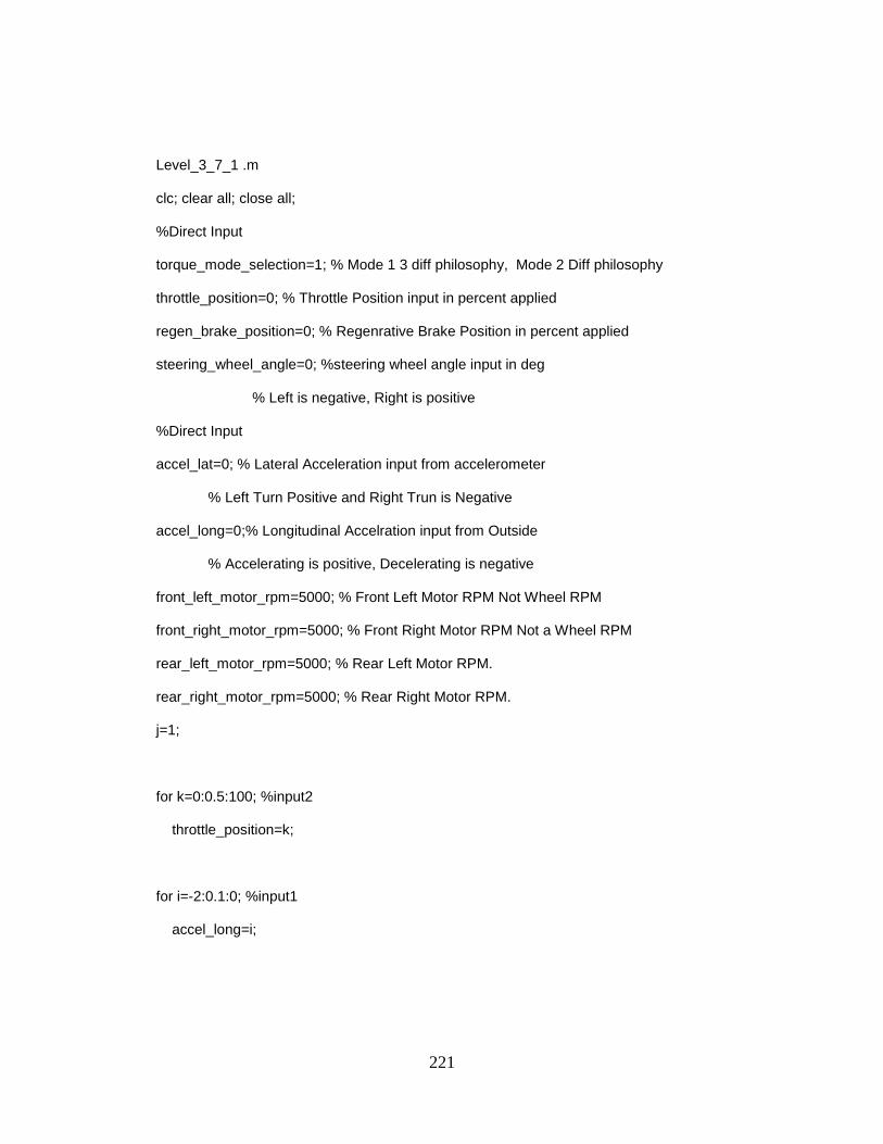
221
Level_3_7_1 .m
clc; clear all; close all;
%Direct Input
torque_mode_selection=1; % Mode 1 3 diff philosophy, Mode 2 Diff philosophy
throttle_position=0; % Throttle Position input in percent applied
regen_brake_position=0; % Regenrative Brake Position in percent applied
steering_wheel_angle=0; %steering wheel angle input in deg
% Left is negative, Right is positive
%Direct Input
accel_lat=0; % Lateral Acceleration input from accelerometer
% Left Turn Positive and Right Trun is Negative
accel_long=0;% Longitudinal Accelration input from Outside
% Accelerating is positive, Decelerating is negative
front_left_motor_rpm=5000; % Front Left Motor RPM Not Wheel RPM
front_right_motor_rpm=5000; % Front Right Motor RPM Not a Wheel RPM
rear_left_motor_rpm=5000; % Rear Left Motor RPM.
rear_right_motor_rpm=5000; % Rear Right Motor RPM.
j=1;
for k=0:0.5:100; %input2
throttle_position=k;
for i=-2:0.1:0; %input1
accel_long=i;

222
% Call E_diff Function to Determine Output to Motor Controllers
[lambda_TV_FL_Regen,lambda_TV_FR_Regen,lambda_TV_RL_Regen,lambda_TV_RR
_Regen,lambda_TV_FL_Throttle, lambda_TV_FR_Throttle, lambda_TV_RL_Throttle,
lambda_TV_RR_Throttle, requested_torque_front_left_motor,
requested_torque_front_right_motor, requested_torque_rear_left_motor,
requested_torque_rear_right_motor, requested_total_torque, torque_front_left_output,
torque_front_right_output, torque_rear_left_output, torque_rear_right_output,
total_output_torque]=E_diff(torque_mode_selection, throttle_position,
regen_brake_position, steering_wheel_angle, accel_lat,accel_long, front_left_motor_rpm,
front_right_motor_rpm, rear_left_motor_rpm, rear_right_motor_rpm);
% Save the lambda_TV outputs into an array
a_array_input1(1,j)=i;
a_array_input2(1,j)=k;
a_newTP_FL(1,j)=lambda_TV_FL_Throttle;
a_newTP_FR(1,j)=lambda_TV_FR_Throttle;
a_newTP_RL(1,j)=lambda_TV_RL_Throttle;
a_newTP_RR(1,j)=lambda_TV_RR_Throttle;
a_newRP_FL(1,j)=lambda_TV_FL_Regen;
a_newRP_FR(1,j)=lambda_TV_FR_Regen;
a_newRP_RL(1,j)=lambda_TV_RL_Regen;

223
a_newRP_RR(1,j)=lambda_TV_RR_Regen;
a_RT_FL(1,j)=requested_torque_front_left_motor;
a_RT_FR(1,j)=requested_torque_front_right_motor;
a_RT_RL(1,j)=requested_torque_rear_left_motor;
a_RT_RR(1,j)=requested_torque_rear_right_motor;
a_RT_total(1,j)=requested_total_torque;
a_VT_FL(1,j)=torque_front_left_output;
a_VT_FR(1,j)=torque_front_right_output;
a_VT_RL(1,j)=torque_rear_left_output;
a_VT_RR(1,j)=torque_rear_right_output;
a_VT_total(1,j)=total_output_torque;
j=j+1;
end
end
figure('Name','Level 3_7','WindowStyle','docked');
subplot(2,2,1)
plot3(a_array_input1, a_array_input2, a_newTP_FL,'g.');
title 'FL'
xlabel 'longitudinal acceleration'
ylabel 'input throttle position'
ylim ([-10,110]);

224
zlabel 'torque vectored throttle position'
zlim ([-10,110]);
grid on
subplot(2,2,2)
plot3(a_array_input1, a_array_input2, a_newTP_FR,'g.');
title 'FR'
xlabel 'longitudinal acceleration'
ylabel 'input throttle position'
ylim ([-10,110]);
zlabel 'torque vectored throttle position'
zlim ([-10,110]);
grid on
subplot(2,2,3)
plot3(a_array_input1,a_array_input2, a_newTP_RL,'g.');
title 'RL'
xlabel 'longitudinal acceleration'
ylabel 'input throttle position'
ylim ([-10,110]);
zlabel 'torque vectored throttle position'
zlim ([-10,110]);
grid on
subplot(2,2,4)

225
plot3(a_array_input1,a_array_input2, a_newTP_RR,'g.');
title 'RR'
xlabel 'longitudinal acceleration'
ylabel 'input throttle position'
ylim ([-10,110]);
zlabel 'torque vectored throttle position'
zlim ([-10,110]);
grid on
figure('Name','Level 3_7','WindowStyle','docked');
subplot(2,2,1)
plot3(a_array_input1, a_array_input2, a_newRP_FL,'r.');
title 'FL'
xlabel 'longitudinal acceleration'
ylabel 'input throttle position'
ylim ([-10,110]);
zlabel 'torque vectored regen position'
zlim ([-10,110]);
grid on
subplot(2,2,2)
plot3(a_array_input1, a_array_input2, a_newRP_FR,'r.');
title 'FR'
xlabel 'longitudinal acceleration'
ylabel 'input throttle position'
ylim ([-10,110]);
226
zlabel 'torque vectored regen position'
zlim ([-10,110]);
grid on
subplot(2,2,3)
plot3(a_array_input1,a_array_input2, a_newRP_RL,'r.');
title 'RL'
xlabel 'longitudinal acceleration'
ylabel 'input throttle position'
ylim ([-10,110]);
zlabel 'torque vectored regen position'
zlim ([-10,110]);
grid on
subplot(2,2,4)
plot3(a_array_input1,a_array_input2, a_newRP_RR,'r.');
title 'RR'
xlabel 'longitudinal acceleration'
ylabel 'input throttle position'
ylim ([-10,110]);
zlabel 'torque vectored regen position'
zlim ([-10,110]);
grid on
figure('Name','Level 3_7','WindowStyle','docked');
subplot(2,2,1)

227
plot3(a_array_input1,a_array_input2, a_RT_FL,'.', a_array_input1, a_array_input2,
a_VT_FL,'.');
title 'FL'
xlabel 'longitudinal acceleration'
ylabel 'input throttle position'
zlabel 'motor torque'
zlim ([-40,40])
grid on
legend ('Requested Torque','VectoredTorque','Location','NorthEast')
subplot(2,2,2)
plot3(a_array_input1,a_array_input2,a_RT_FR,'.', a_array_input1,a_array_input2,
a_VT_FR,'.');
title 'FR'
xlabel 'longitudinal acceleration'
ylabel 'input throttle position'
zlabel 'motor torque'
zlim ([-40,40])
grid on
subplot(2,2,3)
plot3(a_array_input1,a_array_input2,a_RT_RL,'.', a_array_input1,a_array_input2,
a_VT_RL,'.');
title 'RL'
xlabel 'longitudinal acceleration'

228
ylabel 'input throttle position'
zlabel 'motor torque'
zlim ([-40,40])
grid on
subplot(2,2,4)
plot3(a_array_input1,a_array_input2,a_RT_RR,'.', a_array_input1,a_array_input2,
a_VT_RR,'.');
title 'RR'
xlabel 'longitudinal acceleration'
ylabel 'input throttle position'
zlabel 'motor torque'
zlim ([-40,40])
grid on
figure('Name','Level 3_7','WindowStyle','docked');
plot3( a_array_input1,a_array_input2, a_RT_total,'o',a_array_input1,a_array_input2,
a_VT_total,'.');
title 'Total Requested Torque and Total Vectored Torque vs Swept Input'
xlabel 'longitudinal acceleration'
ylabel 'input throttle position'
zlabel 'motor torque'
zlim ([-100,100])
grid on ;legend ('Requested Torque','VectoredTorque','Location','SouthWest')

229
Appendix E
List of Symbols

230
List of Symbols -
xA Longitudinal acceleration
yA Lateral acceleration
sa Distance between sprung mass CG and front axle
b Distance of CG from front axle
c Distance of CG from rear axle
yF Lateral force acting at roll center for single axle
FyF Lateral force acting at roll center for front axle
RyF Lateral force acting at roll center for rear axle
G Gear reduction ratio
h Center of gravity of car with driver
sh Perpendicular distance between CG and roll axis
K Total suspension roll stiffness
SK Suspension spring stiffness
WK Wheel Rate
HK Heave rate
WK Roll stiffness between two wheels
aK Roll stiffness at each axle
FK Effective roll stiffness of front axle
RK Effective roll stiffness of rear axle
l Wheelbase of car
M Roll moment generated around CG
rollM Moment due to roll
sprungrollM Moment due to sprung mass roll
ssUnsprungmaM Moment due to unsprung mass
R Radius of turn
TR Static radius of tire
𝑅𝑃 Regenerative brake pedal position
S Motor Rpm
PeakS Motor’s peak speed

231
PeakfS Front motor peak speed
PeakrS Rear motor peak speed
𝑆𝑚𝑎𝑥 Maximum motor speed at given rpm
𝑆𝑓𝑙 Front left motor rpm
frS Front right motor rpm
rlS Rear left motor rpm
rrS Rear right motor rom
t Average track width
at Track width at axle
Ft Track width at front axle
Rt Track width at rear axle
T Motor torque
PeakT Motor peak torque
𝑇𝑝𝑒𝑎𝑘𝑓 Front motor peak torque
PeakrT Rear motor peak torque
𝑇𝑚𝑎𝑥 Maximum motor torque at given rpm
𝑇𝑓𝑙 Front left driver requested torque
𝑇𝑓𝑟 Front right driver requested torque
𝑇𝑟𝑙 Rear left driver requested torque
𝑇𝑟𝑟 Rear right driver requested torque
𝑇𝑓𝑙100 Front left toque at 100% throttle
𝑇𝑓𝑟100 Front right toque at 100% throttle
𝑇𝑙𝑟100 Rear left toque at 100% throttle
𝑇𝑟𝑟100 Rear right toque at 100% throttle
𝑇𝑃 Throttle position
𝑇𝑟𝑒𝑞𝑢𝑒𝑠𝑡𝑒𝑑𝑓 Driver requested torque from front axle
𝑇𝑟𝑒𝑞𝑢𝑒𝑠𝑡𝑒𝑑𝑟 Driver requested torque from rear axle
SWV Velocity of single wheel
f lV Velocity of front left wheel
frV Velocity of front right wheel
lrV Velocity of rear left wheel
rrV Velocity of rear right wheel

232
𝑉𝑇𝑓𝑙 Front left vectored toqrque
𝑉𝑇𝑓𝑟 Front right vectored torque
𝑉𝑇𝑟𝑙 Rear left vectored torque
𝑉𝑇𝑟𝑟 Rear right vectored torque
fW Total normal load on front axle
rW Total normal load on rear axle
f lW Total normal load on front left
frW Total normal load on front right
rlW Total normal load on rear left
rrW Total normal load on rear right
SW Sprung mass
SFW Sprung mass on front axle
SRW Sprung mass on rear axle
SsaW Sprung mass at single axle
W Total lateral load transfer
FW Lateral load transfer at front axle
RW Lateral load transfer at rear axle
oW Normal load on outside wheel
iW Normal load on inside wheel
W Weight of Car
LW Total normal load on left wheels
RW Total normal load on right wheels
uaW Unsprung mass at single axle
RaZ Roll center height for single axle
RFZ Roll center height for front suspension
RRZ Roll center height for rear suspension
uaZ Unsprung mass CG height at single axle
i Inside wheel steering angle
Chassis roll angle
ƛ𝑡ℎ𝑟𝑜𝑡𝑡𝑙𝑒𝑓𝑙 Front left torque vectored throttle position output
ƛ𝑡ℎ𝑟𝑜𝑡𝑡𝑙𝑒𝑓𝑟 Front right torque vectored throttle position output
ƛ𝑡ℎ𝑟𝑜𝑡𝑡𝑙𝑒𝑟𝑙 Rear left torque vectored throttle position output
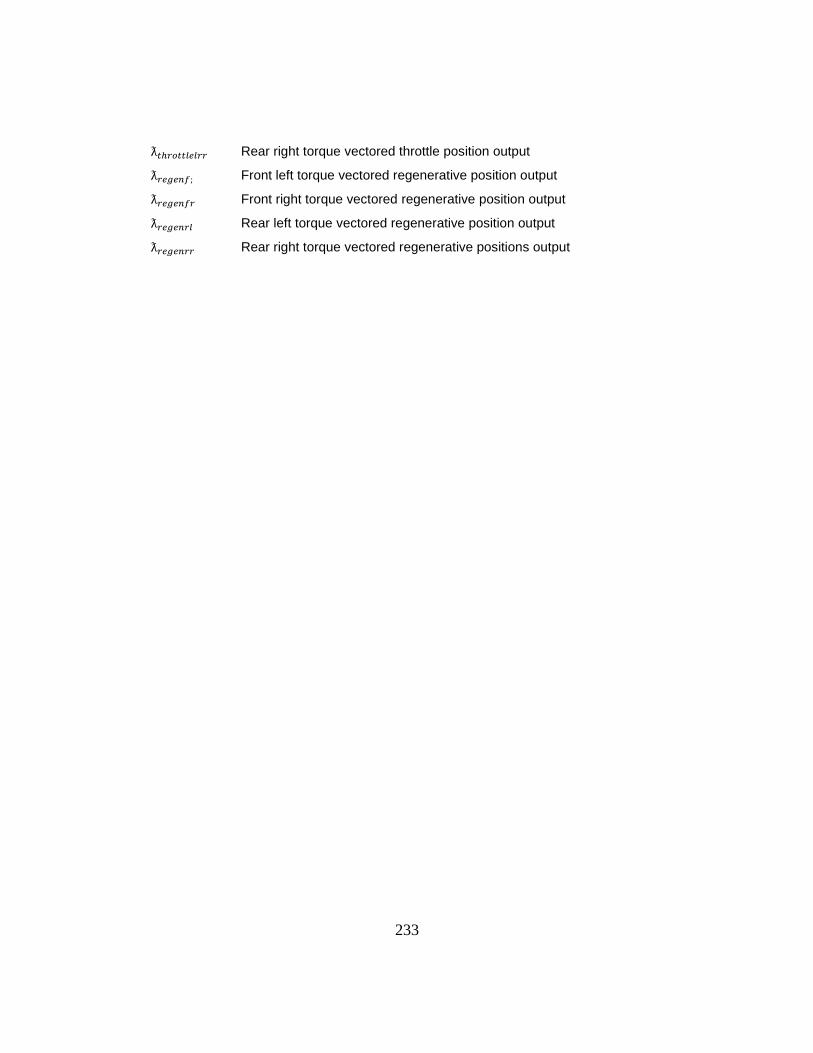
233
ƛ𝑡ℎ𝑟𝑜𝑡𝑡𝑙𝑒𝑙𝑟𝑟 Rear right torque vectored throttle position output
ƛ𝑟𝑒𝑔𝑒𝑛𝑓; Front left torque vectored regenerative position output
ƛ𝑟𝑒𝑔𝑒𝑛𝑓𝑟 Front right torque vectored regenerative position output
ƛ𝑟𝑒𝑔𝑒𝑛𝑟𝑙 Rear left torque vectored regenerative position output
ƛ𝑟𝑒𝑔𝑒𝑛𝑟𝑟 Rear right torque vectored regenerative positions output

234
References
Fundamentals of Vehicle Dynamics Thomos D. Gillespie
Race Car Vehicle Dynamics: William F Milliken and Douglas L. Milliken
Figure 2-1: Source unknown.

235

236
Biographical Information
Vikas Pawar has master of science degree in Mechanical Engineering from The
University of Texas at Arlington in 2016, Texas, USA. He has earned his Bachelor degree
in Mechanical Engineering from University of Mumbai in 2012. He has been done is high
school education till 2008 in Phaltan, Maharashtra India.
Vikas has been associated with FSAE in between 2009-2012 on formula student
team Orion racing India(ORI). There he has worked on Chassis and bodywork in between
2009-2011. He worked as a chassis system lead for ORI’s 2012 car. He did is final year
undergraduate project on “ Design and Manufacturing of Automobile Chassis’ He was
working at Tenova Metals India, Mumbai as a Sales and Proposal Engineer from July 2012-
July 2014.
He joined a UTA in August 2014 as a graduate Master student and got associated
with Formula student team UTA Racing since December 2014. He took responsibility of
designing torque-vectoring system for UTA racing and decided to pursue it as his thesis
research study. His master study interest had targeted towards design and controls. He
did his internship at CTJ Energy Solution as a Mechanical Engineering intern.
Vikas research interest involves vehicle dynamics, transient vehicle dynamics ,
mathematical modelling ,suspension design, vehicle test data analysis and dynamic
control. He has completed his thesis study in August 2016 and graduated from UTA.
He is hoping to pursue his career in Vehicle Dynamics and autonomous driving.
He would going to work at Robert Bosch LLC. , Plymouth ,Michigan as an Associate
software Engineer in chassis control division, from August 2016.