Heavier equipment with faster machine speeds coupled with higher costs have made rule-of-thumb

approaches and "rigid structure" assumptions either unsafe or too conservative for the design of many

structures with vibrating machinery. SAP2000 can easily compute natural frequencies, deformations and

forces in the structure with consideration of structure mass and flexibility. Using less rigorous design

approaches, these factors are either ignored, conservatively assumed, or handled in a simplified

approximate fashion. Sizing and design of a skid or foundation supporting vibrating equipment is beyond the

scope of this tutorial. However, here are a few considerations:

• Run multiple analyses which vary soil spring constants and damping ratio to account for uncertainties

of soil data.

• Acting frequency of the vibrating machinery should not be close to the structure’s resonant frequency

• Dynamic effects to and from adjoining structures and equipment. Modular skids may be designed in

isolation for vibrating equipment. Yet these skids can be added to other parts of a larger structure

which may change the initial design assumptions.

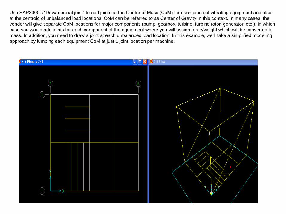
Use SAP2000’s “Draw special joint” to add joints at the Center of Mass (CoM) for each piece of vibrating equipment and also

at the centroid of unbalanced load locations. CoM can be referred to as Center of Gravity in this context. In many cases, the

vendor will give separate CoM locations for major components (pump, gearbox, turbine, turbine rotor, generator, etc.), in which

case you would add joints for each component of the equipment where you will assign force/weight which will be converted to

mass. In addition, you need to draw a joint at each unbalanced load location. In this example, we’ll take a simplified modeling

approach by lumping each equipment CoM at just 1 joint location per machine.

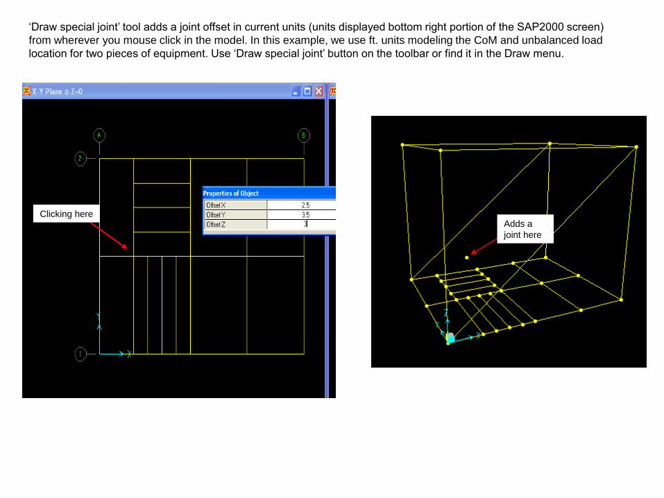
Clicking here Adds a

joint here

‘Draw special joint’ tool adds a joint offset in current units (units displayed bottom right portion of the SAP2000 screen)

from wherever you mouse click in the model. In this example, we use ft. units modeling the CoM and unbalanced load

location for two pieces of equipment. Use ‘Draw special joint’ button on the toolbar or find it in the Draw menu.

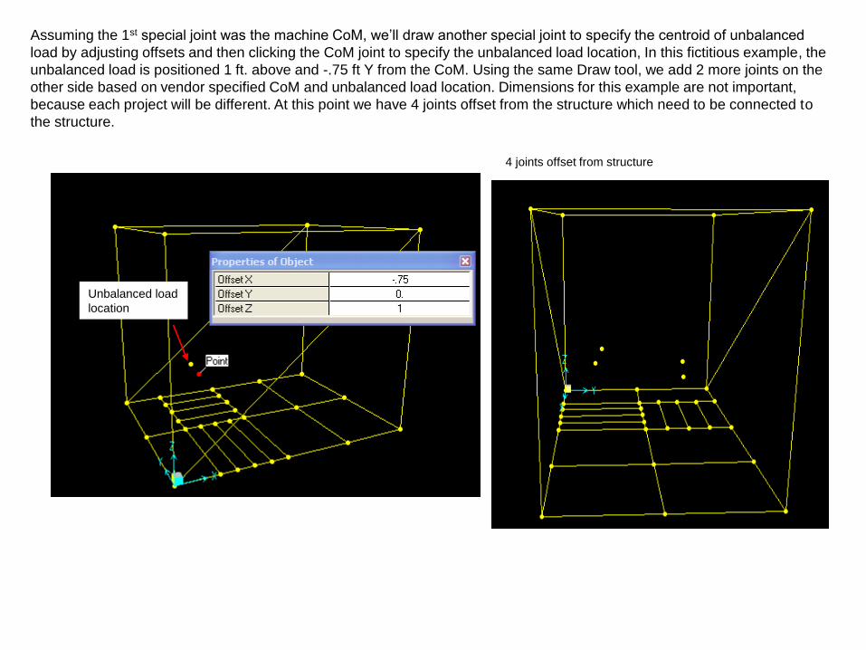
Assuming the 1st special joint was the machine CoM, we’ll draw another special joint to specify the centroid of unbalanced

load by adjusting offsets and then clicking the CoM joint to specify the unbalanced load location, In this fictitious example, the

unbalanced load is positioned 1 ft. above and -.75 ft Y from the CoM. Using the same Draw tool, we add 2 more joints on the

other side based on vendor specified CoM and unbalanced load location. Dimensions for this example are not important,

because each project will be different. At this point we have 4 joints offset from the structure which need to be connected to

the structure.

Unbalanced load

location

4 joints offset from structure

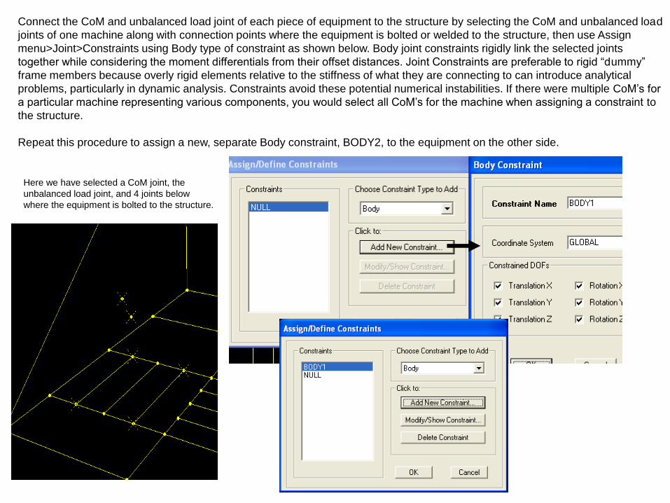
Here we have selected a CoM joint, the

unbalanced load joint, and 4 joints below

where the equipment is bolted to the structure.

Connect the CoM and unbalanced load joint of each piece of equipment to the structure by selecting the CoM and unbalanced load

joints of one machine along with connection points where the equipment is bolted or welded to the structure, then use Assign

menu>Joint>Constraints using Body type of constraint as shown below. Body joint constraints rigidly link the selected joints

together while considering the moment differentials from their offset distances. Joint Constraints are preferable to rigid “dummy”

frame members because overly rigid elements relative to the stiffness of what they are connecting to can introduce analytical

problems, particularly in dynamic analysis. Constraints avoid these potential numerical instabilities. If there were multiple CoM’s for

a particular machine representing various components, you would select all CoM’s for the machine when assigning a constraint to

the structure.

Repeat this procedure to assign a new, separate Body constraint, BODY2, to the equipment on the other side.

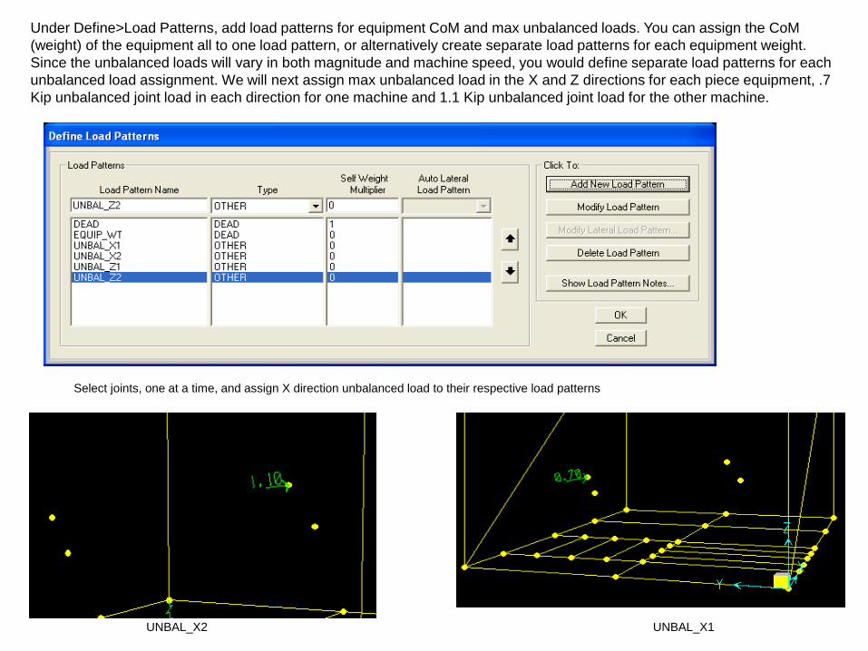
Under Define>Load Patterns, add load patterns for equipment CoM and max unbalanced loads. You can assign the CoM

(weight) of the equipment all to one load pattern, or alternatively create separate load patterns for each equipment weight.

Since the unbalanced loads will vary in both magnitude and machine speed, you would define separate load patterns for each

unbalanced load assignment. We will next assign max unbalanced load in the X and Z directions for each piece equipment, .7

Kip unbalanced joint load in each direction for one machine and 1.1 Kip unbalanced joint load for the other machine.

Select joints, one at a time, and assign X direction unbalanced load to their respective load patterns

UNBAL_X1 UNBAL_X2

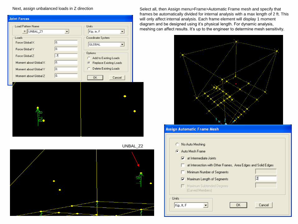
Select all, then Assign menu>Frame>Automatic Frame mesh and specify that

frames be automatically divided for internal analysis with a max length of 2 ft. This

will only affect internal analysis. Each frame element will display 1 moment

diagram and be designed using it’s physical length. For dynamic analysis,

meshing can affect results. It’s up to the engineer to determine mesh sensitivity.

UNBAL_Z2

Next, assign unbalanced loads in Z direction

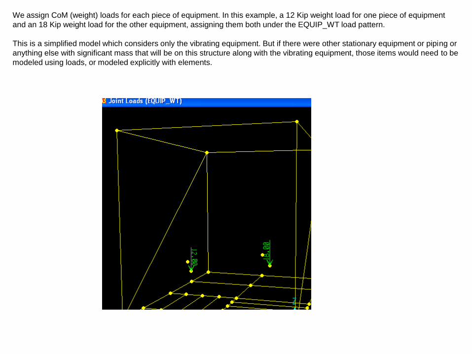
We assign CoM (weight) loads for each piece of equipment. In this example, a 12 Kip weight load for one piece of equipment

and an 18 Kip weight load for the other equipment, assigning them both under the EQUIP_WT load pattern.

This is a simplified model which considers only the vibrating equipment. But if there were other stationary equipment or piping or

anything else with significant mass that will be on this structure along with the vibrating equipment, those items would need to be

modeled using loads, or modeled explicitly with elements.

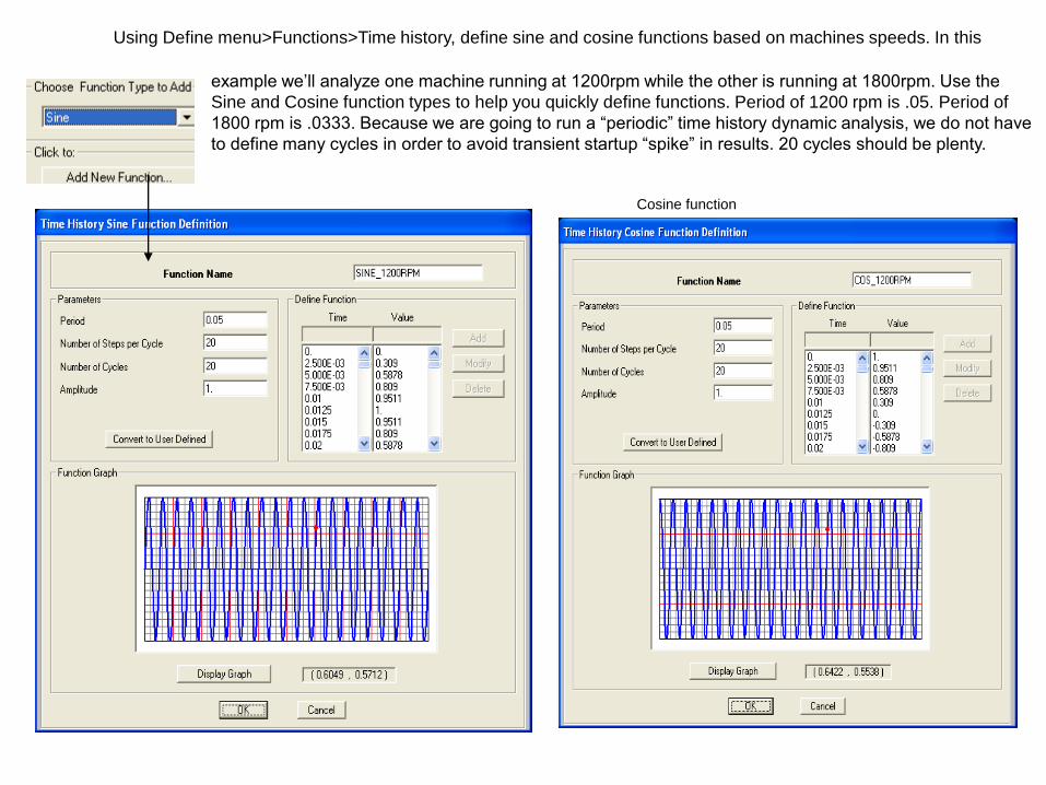
Using Define menu>Functions>Time history, define sine and cosine functions based on machines speeds. In this

example we’ll analyze one machine running at 1200rpm while the other is running at 1800rpm. Use the

Sine and Cosine function types to help you quickly define functions. Period of 1200 rpm is .05. Period of

1800 rpm is .0333. Because we are going to run a “periodic” time history dynamic analysis, we do not have

to define many cycles in order to avoid transient startup “spike” in results. 20 cycles should be plenty.

Cosine function

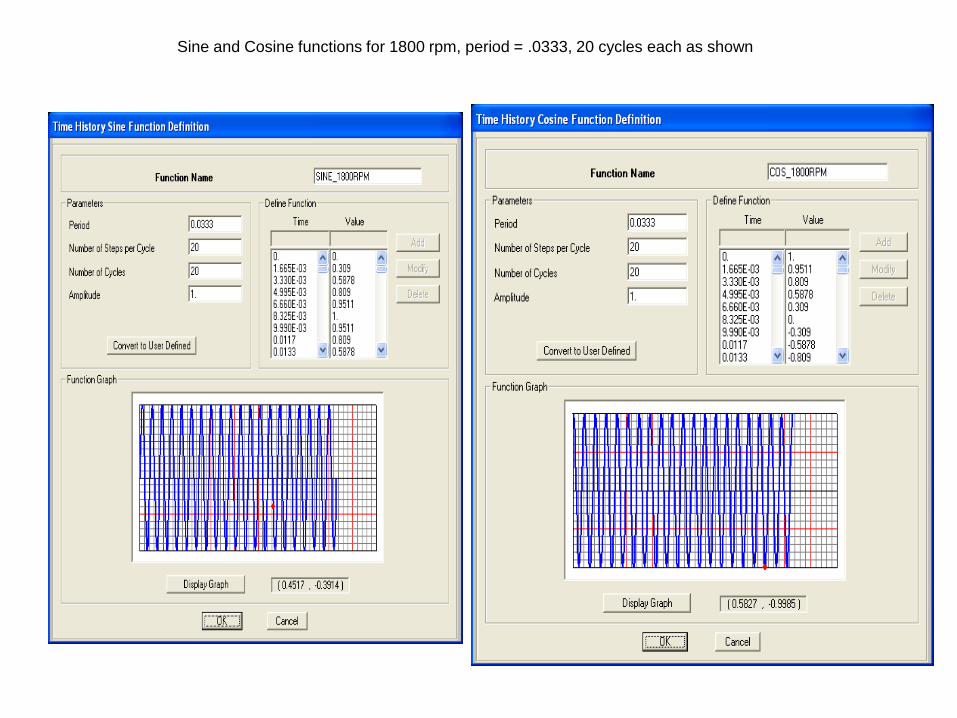
Sine and Cosine functions for 1800 rpm, period = .0333, 20 cycles each as shown

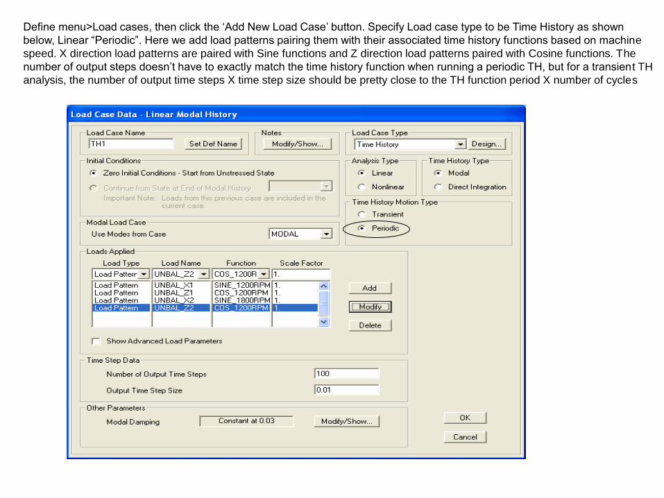
Define menu>Load cases, then click the ‘Add New Load Case’ button. Specify Load case type to be Time History as shown

below, Linear “Periodic”. Here we add load patterns pairing them with their associated time history functions based on machine

speed. X direction load patterns are paired with Sine functions and Z direction load patterns paired with Cosine functions. The

number of output steps doesn’t have to exactly match the time history function when running a periodic TH, but for a transient TH

analysis, the number of output time steps X time step size should be pretty close to the TH function period X number of cycles

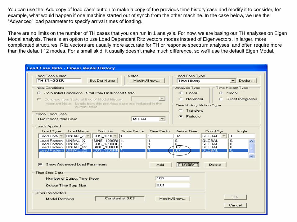
You can use the ‘Add copy of load case’ button to make a copy of the previous time history case and modify it to consider, for

example, what would happen if one machine started out of synch from the other machine. In the case below, we use the

“Advanced” load parameter to specify arrival times of loading.

There are no limits on the number of TH cases that you can run in 1 analysis. For now, we are basing our TH analyses on Eigen

Modal analysis. There is an option to use Load Dependent Ritz vectors modes instead of Eigenvectors. In larger, more

complicated structures, Ritz vectors are usually more accurate for TH or response spectrum analyses, and often require more

than the default 12 modes. For a small skid, it usually doesn’t make much difference, so we’ll use the default Eigen Modal.

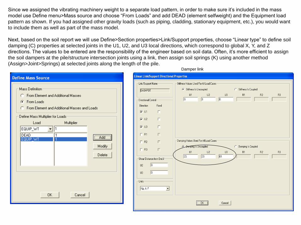
Since we assigned the vibrating machinery weight to a separate load pattern, in order to make sure it’s included in the mass

model use Define menu>Mass source and choose “From Loads” and add DEAD (element selfweight) and the Equipment load

pattern as shown. If you had assigned other gravity loads (such as piping, cladding, stationary equipment, etc.), you would want

to include them as well as part of the mass model.

Next, based on the soil report we will use Define>Section properties>Link/Support properties, choose “Linear type” to define soil

damping (C) properties at selected joints in the U1, U2, and U3 local directions, which correspond to global X, Y, and Z

directions. The values to be entered are the responsibility of the engineer based on soil data. Often, it’s more efficient to assign

the soil dampers at the pile/structure intersection joints using a link, then assign soil springs (K) using another method

(Assign>Joint>Springs) at selected joints along the length of the pile. Damper link

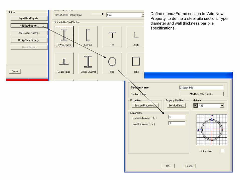
Define menu>Frame section to ‘Add New

Property’ to define a steel pile section. Type

diameter and wall thickness per pile

specifications.

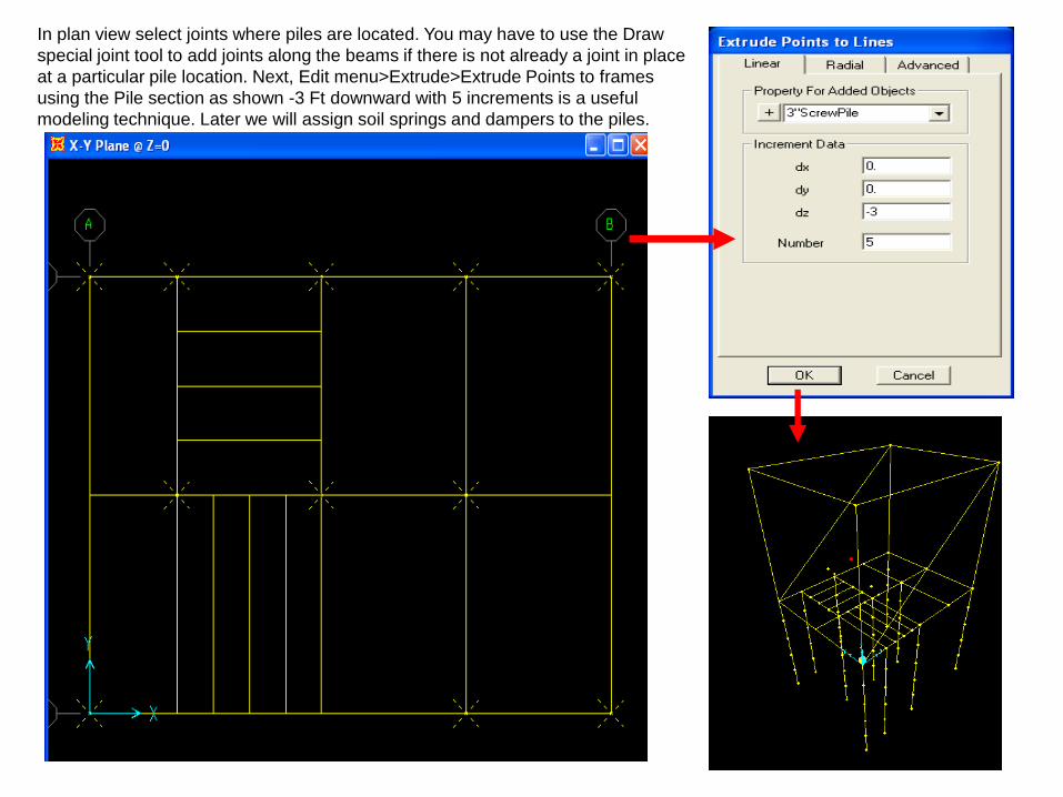
In plan view select joints where piles are located. You may have to use the Draw

special joint tool to add joints along the beams if there is not already a joint in place

at a particular pile location. Next, Edit menu>Extrude>Extrude Points to frames

using the Pile section as shown -3 Ft downward with 5 increments is a useful

modeling technique. Later we will assign soil springs and dampers to the piles.

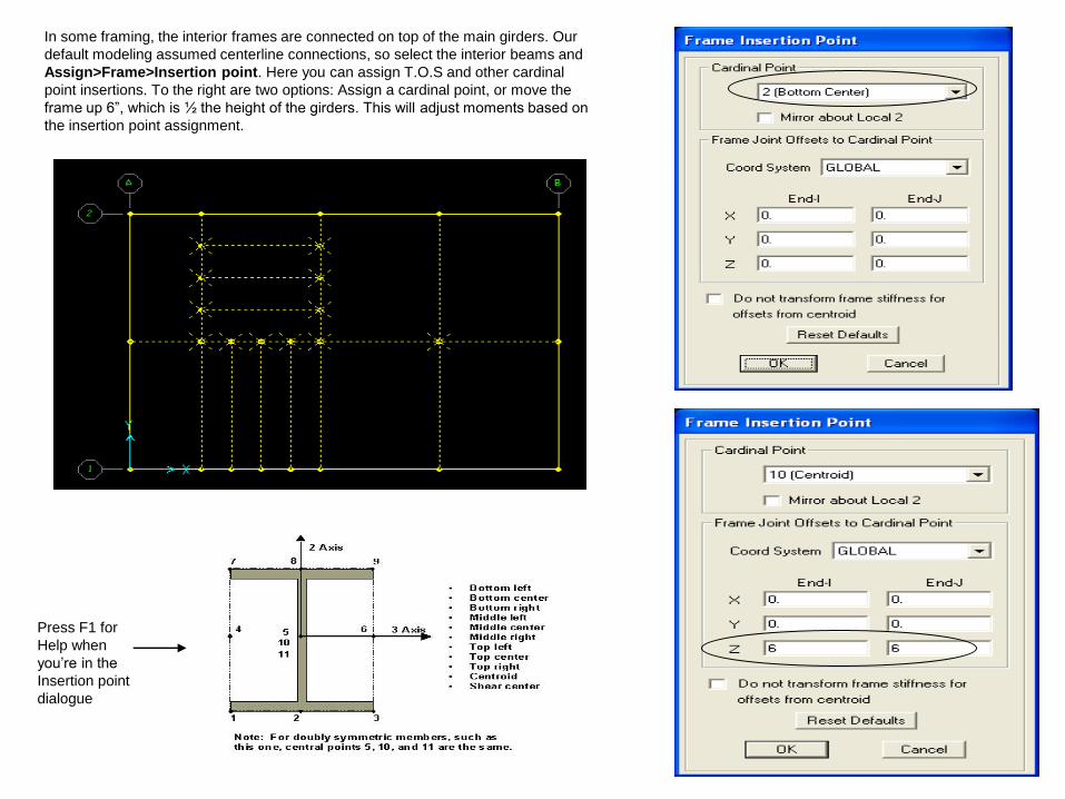
In some framing, the interior frames are connected on top of the main girders. Our

default modeling assumed centerline connections, so select the interior beams and

Assign>Frame>Insertion point. Here you can assign T.O.S and other cardinal

point insertions. To the right are two options: Assign a cardinal point, or move the

frame up 6”, which is ½ the height of the girders. This will adjust moments based on

the insertion point assignment.

Press F1 for

Help when

you’re in the

Insertion point

dialogue

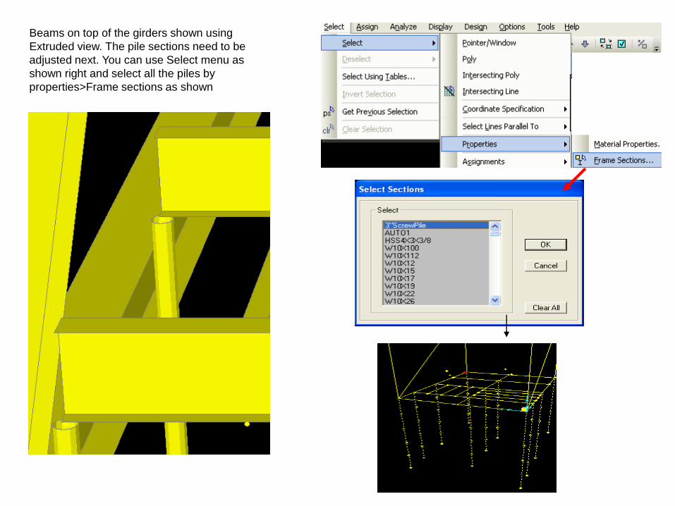
Beams on top of the girders shown using

Extruded view. The pile sections need to be

adjusted next. You can use Select menu as

shown right and select all the piles by

properties>Frame sections as shown

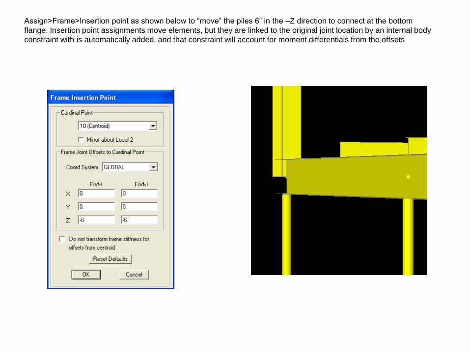
Assign>Frame>Insertion point as shown below to “move” the piles 6” in the –Z direction to connect at the bottom

flange. Insertion point assignments move elements, but they are linked to the original joint location by an internal body

constraint with is automatically added, and that constraint will account for moment differentials from the offsets

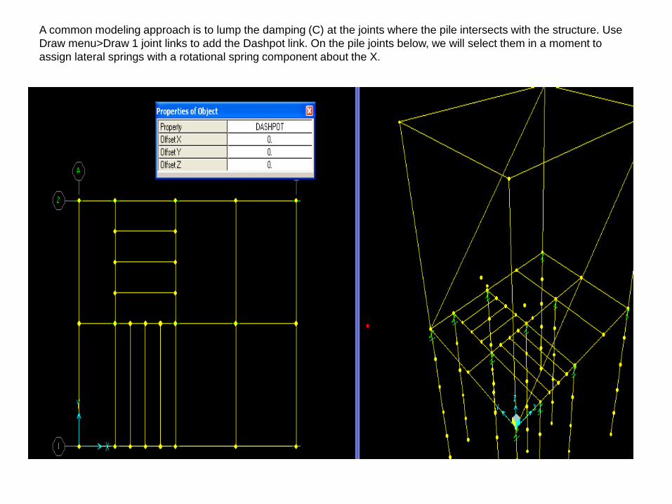
A common modeling approach is to lump the damping (C) at the joints where the pile intersects with the structure. Use

Draw menu>Draw 1 joint links to add the Dashpot link. On the pile joints below, we will select them in a moment to

assign lateral springs with a rotational spring component about the X.

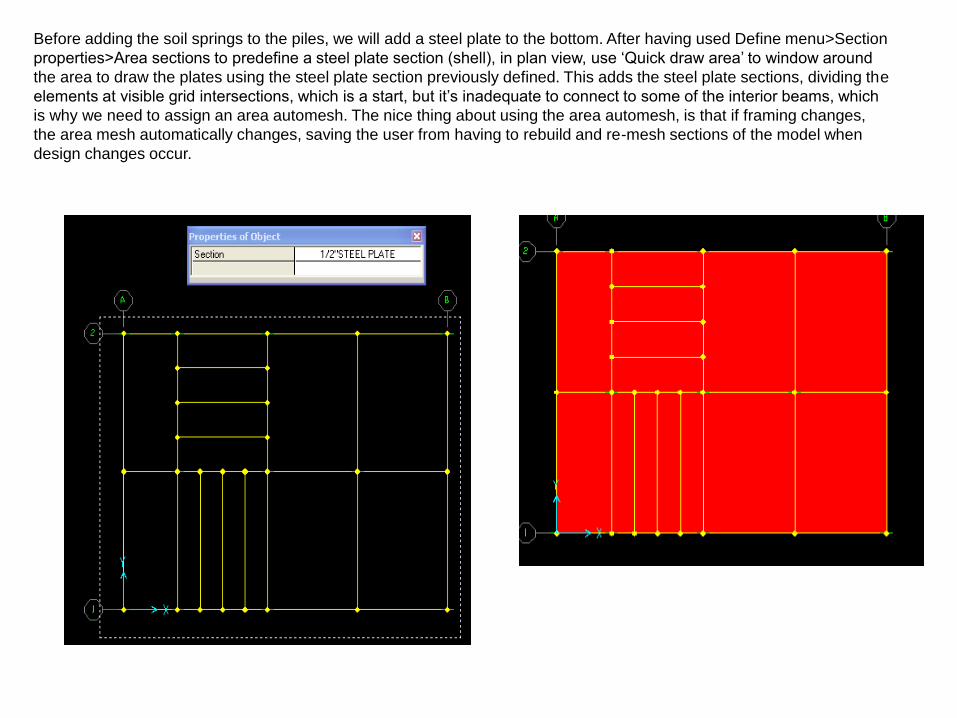
Before adding the soil springs to the piles, we will add a steel plate to the bottom. After having used Define menu>Section

properties>Area sections to predefine a steel plate section (shell), in plan view, use ‘Quick draw area’ to window around

the area to draw the plates using the steel plate section previously defined. This adds the steel plate sections, dividing the

elements at visible grid intersections, which is a start, but it’s inadequate to connect to some of the interior beams, which

is why we need to assign an area automesh. The nice thing about using the area automesh, is that if framing changes,

the area mesh automatically changes, saving the user from having to rebuild and re-mesh sections of the model when

design changes occur.

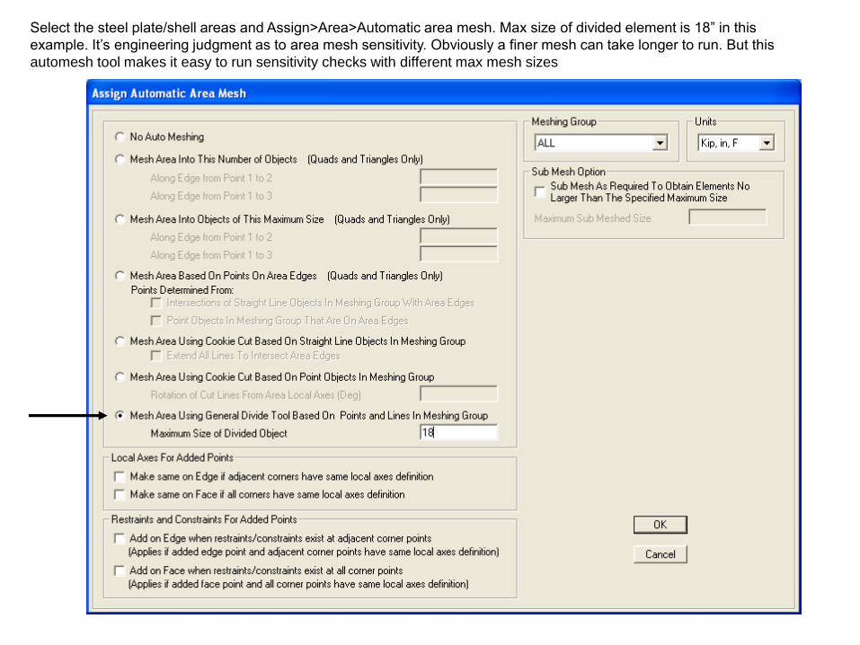
Select the steel plate/shell areas and Assign>Area>Automatic area mesh. Max size of divided element is 18” in this

example. It’s engineering judgment as to area mesh sensitivity. Obviously a finer mesh can take longer to run. But this

automesh tool makes it easy to run sensitivity checks with different max mesh sizes

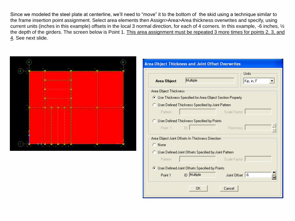
Since we modeled the steel plate at centerline, we’ll need to “move” it to the bottom of the skid using a technique similar to

the frame insertion point assignment. Select area elements then Assign>Area>Area thickness overwrites and specify, using

current units (inches in this example) offsets in the local 3 normal direction, for each of 4 corners. In this example, -6 inches, ½

the depth of the girders. The screen below is Point 1. This area assignment must be repeated 3 more times for points 2, 3, and

4. See next slide.

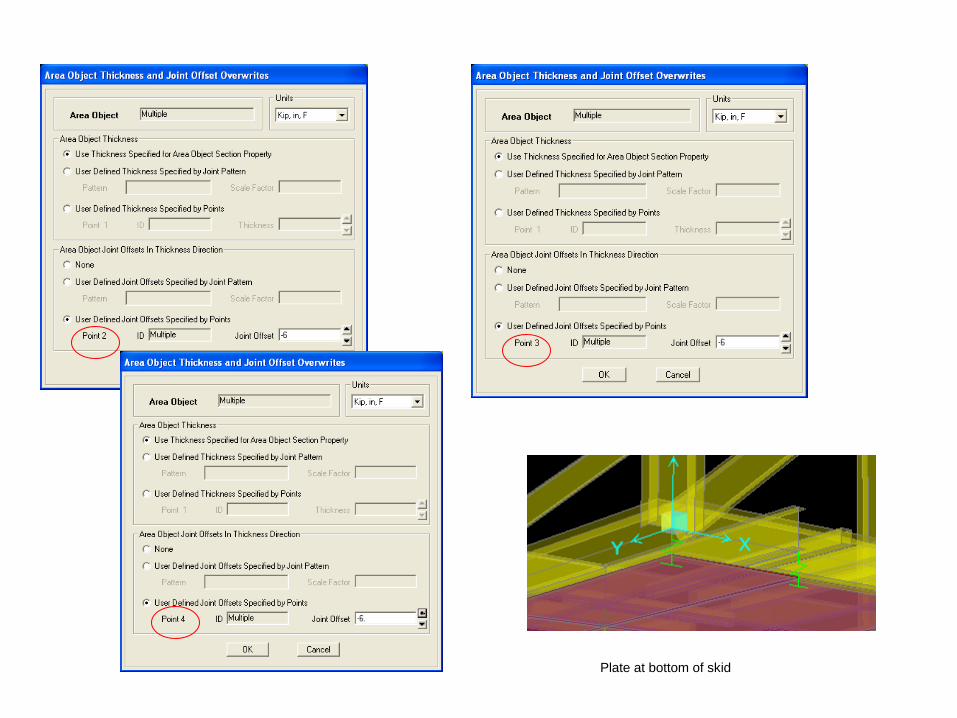
Plate at bottom of skid

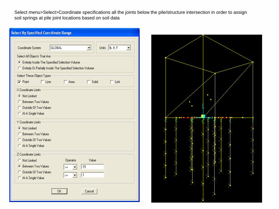
Select menu>Select>Coordinate specifications all the joints below the pile/structure intersection in order to assign

soil springs at pile joint locations based on soil data

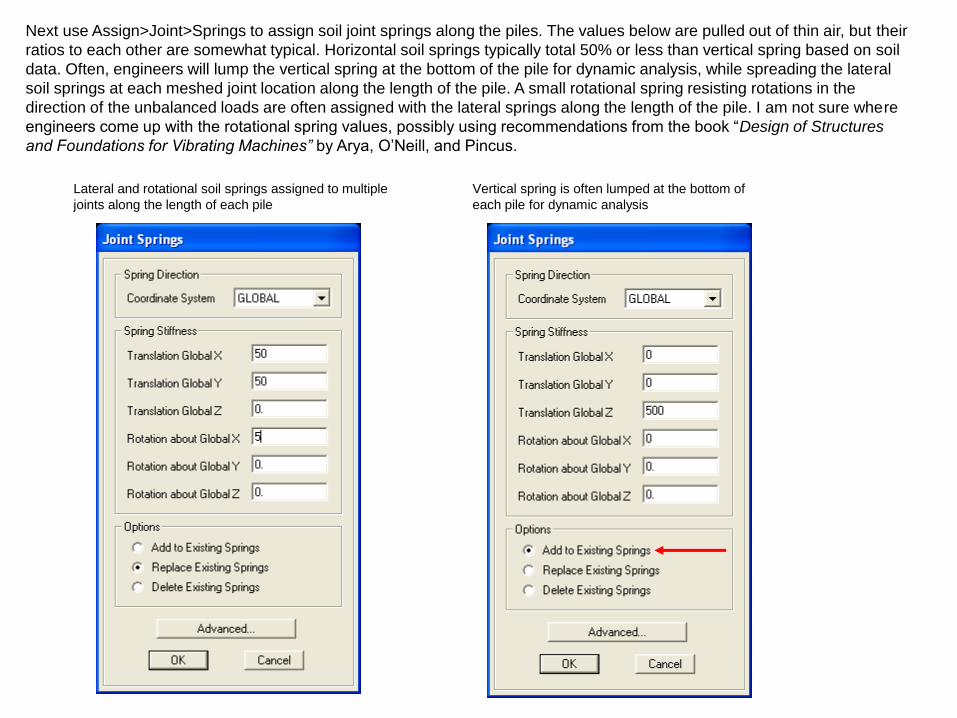
Next use Assign>Joint>Springs to assign soil joint springs along the piles. The values below are pulled out of thin air, but their

ratios to each other are somewhat typical. Horizontal soil springs typically total 50% or less than vertical spring based on soil

data. Often, engineers will lump the vertical spring at the bottom of the pile for dynamic analysis, while spreading the lateral

soil springs at each meshed joint location along the length of the pile. A small rotational spring resisting rotations in the

direction of the unbalanced loads are often assigned with the lateral springs along the length of the pile. I am not sure where

engineers come up with the rotational spring values, possibly using recommendations from the book “Design of Structures

and Foundations for Vibrating Machines” by Arya, O’Neill, and Pincus.

Vertical spring is often lumped at the bottom of

each pile for dynamic analysis

Lateral and rotational soil springs assigned to multiple

joints along the length of each pile

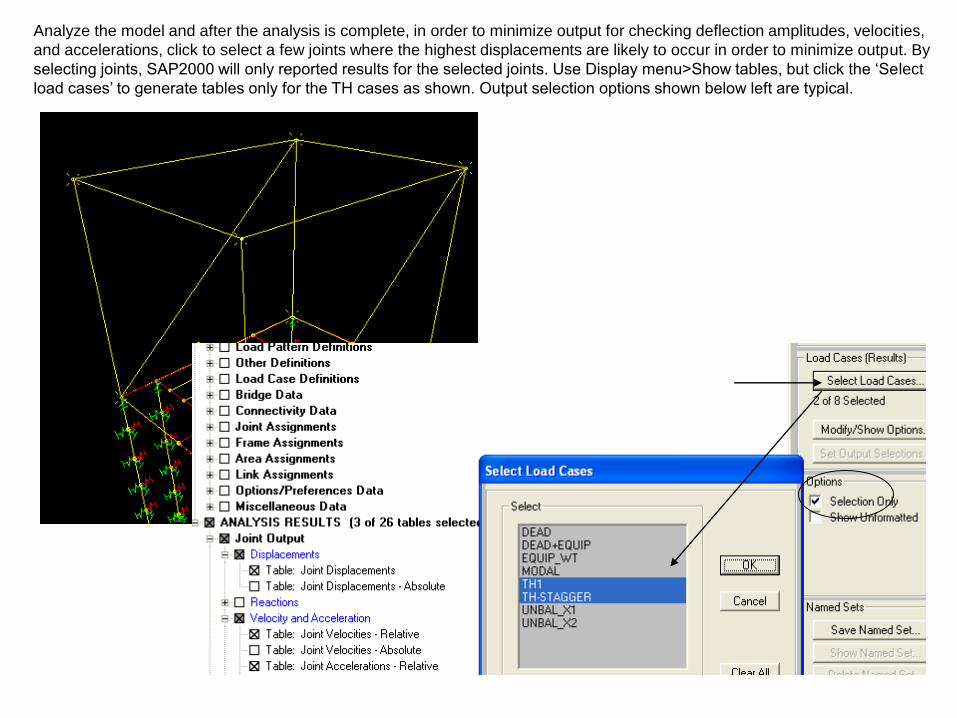
Analyze the model and after the analysis is complete, in order to minimize output for checking deflection amplitudes, velocities,

and accelerations, click to select a few joints where the highest displacements are likely to occur in order to minimize output. By

selecting joints, SAP2000 will only reported results for the selected joints. Use Display menu>Show tables, but click the ‘Select

load cases’ to generate tables only for the TH cases as shown. Output selection options shown below left are typical.

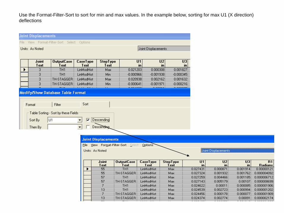
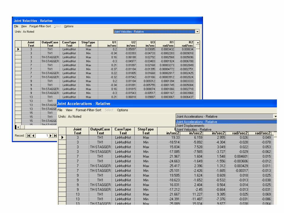
Use the Format-Filter-Sort to sort for min and max values. In the example below, sorting for max U1 (X direction)

deflections

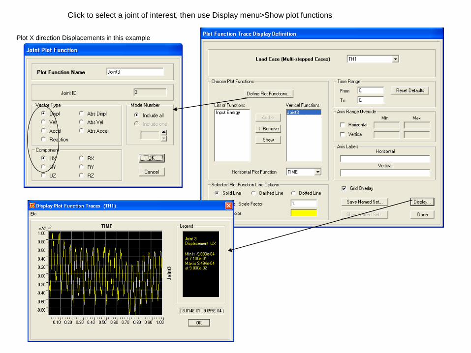
Click to select a joint of interest, then use Display menu>Show plot functions

Plot X direction Displacements in this example

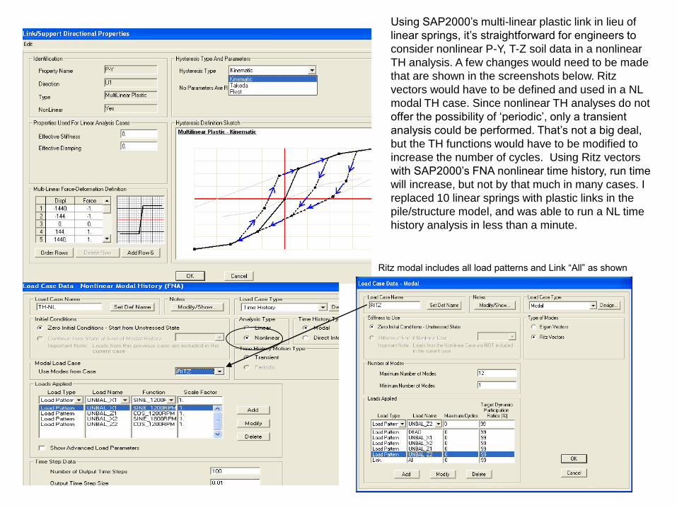
Using SAP2000’s multi-linear plastic link in lieu of

linear springs, it’s straightforward for engineers to

consider nonlinear P-Y, T-Z soil data in a nonlinear

TH analysis. A few changes would need to be made

that are shown in the screenshots below. Ritz

vectors would have to be defined and used in a NL

modal TH case. Since nonlinear TH analyses do not

offer the possibility of ‘periodic’, only a transient

analysis could be performed. That’s not a big deal,

but the TH functions would have to be modified to

increase the number of cycles. Using Ritz vectors

with SAP2000’s FNA nonlinear time history, run time

will increase, but not by that much in many cases. I

replaced 10 linear springs with plastic links in the

pile/structure model, and was able to run a NL time

history analysis in less than a minute.

Ritz modal includes all load patterns and Link “All” as shown