acoustic absorption and the unsteady flow associated … · acoustic absorption and the unsteady...
TRANSCRIPT

Loughborough UniversityInstitutional Repository
Acoustic absorption and theunsteady flow associated
with circular apertures in agas turbine environment
This item was submitted to Loughborough University's Institutional Repositoryby the/an author.
Additional Information:
• A Doctoral Thesis. Submitted in partial fulfilment of the requirementsfor the award of Doctor of Philosophy of Loughborough University.
Metadata Record: https://dspace.lboro.ac.uk/2134/12984
Publisher: c© Jochen Rupp
Please cite the published version.

This item was submitted to Loughborough University as a PhD thesis by the author and is made available in the Institutional Repository
(https://dspace.lboro.ac.uk/) under the following Creative Commons Licence conditions.
For the full text of this licence, please go to: http://creativecommons.org/licenses/by-nc-nd/2.5/

ACOUSTIC ABSORPTION AND THE UNSTEADY FLOW ASSOCIATED WITH CIRCULAR
APERTURES IN A GAS TURBINE ENVIRONMENT
Jochen Rupp
A doctoral Thesis
Submitted in partial fulfilment of requirements for the award of Doctor of Philosophy of Loughborough University
May 2013
© J Rupp 2013

Abstract This work is concerned with the fluid dynamic processes and the associated loss of
acoustic energy produced by circular apertures within noise absorbing perforated walls.
Although applicable to a wide range of engineering applications particular emphasis in
this work is placed on the use of such features within a gas turbine combustion system.
The primary aim for noise absorbers in gas turbine combustion systems is the
elimination of thermo-acoustic instabilities, which are characterised by rapidly rising
pressure amplitudes which are potentially damaging to the combustion system
components. By increasing the amount of acoustic energy being absorbed the
occurrence of thermo-acoustic instabilities can be avoided.
The fundamental acoustic characteristics relating to linear acoustic absorption are
presented. It is shown that changes in orifice geometry, in terms of gas turbine
combustion system representative length-to-diameter ratios, result in changes in the
measured Rayleigh Conductivity. Furthermore in the linear regime the maximum
possible acoustic energy absorption for a given cooling mass flow budget of a
conventional combustor wall will be identified. An investigation into current Rayleigh
Conductivity and aperture impedance (1D) modelling techniques are assessed and the
ranges of validity for these modelling techniques will be identified. Moreover possible
improvements to the modelling techniques are discussed. Within a gas turbine system
absorption can also occur in the non-linear operating regime. Hence the influence of the
orifice geometry upon the optimum non-linear acoustic absorption is also investigated.
Furthermore the performance of non-linear acoustic absorption modelling techniques is
evaluated against the conducted measurements. As the amplitudes within the
combustion system increase the acoustic absorption will transition from the linear to the
non-linear regime. This is important for the design of absorbers or cooling geometries
for gas turbine combustion systems as the propensity for hot gas ingestion increases.
Hence the relevant parameters and phenomena are investigated during the transition
process from linear to non-linear acoustic absorption.
The unsteady velocity field during linear and non-linear acoustic absorption is
captured using particle image velocimetry. A novel analysis technique is developed

Abstract ii
which enables the identification of the unsteady flow field associated with the acoustic
absorption. In this way an investigation into the relevant mechanisms within the
unsteady flow fields to describe the acoustic absorption behaviour of the investigated
orifice plates is conducted. This methodology will also help in the development and
optimisation of future damping systems and provide validation for more sophisticated
3D numerical modelling methods.
Finally a set of design tools developed during this work will be discussed which
enable a comprehensive preliminary design of non-resonant and resonant acoustic
absorbers with multiple perforated liners within a gas turbine combustion system. The
tool set is applied to assess the impact of the gas turbine combustion system space
envelope, complex swirling flow fields and the propensity to hot gas ingestion in the
preliminary design stages.
Keywords: Acoustic Absorption, Rayleigh Conductivity, Impedance, Gas Turbine
Engine, Combustion System, Passive Damping, Thermo-Acoustic Instability, Particle
Image Velocimetry, Proper Orthogonal Decomposition.

Acknowledgement iii
Acknowledgement This thesis has been conducted on a part-time basis at Loughborough University
whilst I am employed by Rolls-Royce. First of all I would like to thank Lesley Hawkins
and Ken Young at Rolls-Royce for giving me the opportunity of conducting this
research at Loughborough University. Special thanks goes to John Moran who in
addition to supporting my application to undertake the research also took the role of my
industrial mentor providing invaluable advice and guidance throughout this work. A big
thank you goes to Michael Spooner and Michael Whiteman of the Combustion and
Casings Engineering Department at Rolls-Royce for their support throughout my thesis
by ensuring I could spend sufficient time away from Rolls-Royce during my studies at
Loughborough University. Without the support from Rolls-Royce this thesis would not
have been possible and this is much appreciated. The support from Rolls-Royce
Deutschland, in particular Sermed Sadig, Miklós Gerendás and Waldemar Lazik is
gratefully acknowledged.
I would like to thank every member of the Rolls-Royce University Technology Centre
at Loughborough University. They provided a great working atmosphere in which
colleagues became friends. A special mention is required for my supervisor Jon Carrotte
for his never ending advice, support, guidance, patience and encouragement throughout
this work. I hope I will get many opportunities in the future to show Jon that my golf
handicap has still not improved. Many thanks to Adrian Spencer for his invaluable
support as well as the support provided to me by Jim McGuirk. I would like to thank
Duncan Walker and Ashley Barker for their continuous encouragement throughout my
research both inside and outside the tearoom. The help from Tim Bradley and Vivek
Savarianandan during the non-resonating liner experiments is also gratefully
acknowledged. I want to thank the technicians for the excellent work on the
experimental test facility, drilling a large amount of holes whenever required.
This thesis is dedicated to my wife Maria and my parents, Rudolf and Elfriede who
are always there for me, with patience and encouragement without which this work
would not have been achieved.

Table of Contents iv
Table of Contents
Abstract i
Acknowledgement iii
Table of Contents iv
List of Figures ix
Nomenclature xix
1 Introduction 1
1.1 Gas Turbine Combustion Systems 1
1.1.1 Environmental Aspects of Gas Turbine Combustion Systems 3
1.2 Thermo-Acoustic Instability 9
1.3 Passive Control of Thermo-Acoustic Instabilities 13
1.3.1 Helmholtz Resonators 14
1.3.2 Multi-Aperture Perforated Screens with Mean Flow 24
1.4 Objectives 33
2 Fundamentals of Unsteady Flow through a Circular Orifice 37
2.1 Steady State Flows through Circular Orifice Plates 37
2.2 Naturally Occurring Phenomena in Unsteady Circular Jet Flow 41
2.3 Forced Unsteady Phenomena in Circular Jet Flow 43
2.3.1 Low Amplitude Forcing 44
2.3.2 High Amplitude Forcing (Vortex Rings) 44
2.4 Fundamentals of Acoustics 48
2.4.1 The Acoustic Wave Equation 48
2.4.2 Plane Acoustic Waves 49
2.4.3 Acoustic Energy Flux 51
2.4.4 Acoustic Absorption Coefficient 51
2.5 Aero-Acoustic Considerations 52

Table of Contents v
2.5.1 The Rayleigh Conductivity 52
2.5.2 Modifications to the Rayleigh Conductivity Model 57
2.5.3 Non-Linear Absorption Modelling 59
3 Experimental Facilities and Methods 65
3.1 Scaling from Gas Turbine Engines to Experimental Test Rig Geometry 67
3.2 Fundamental Investigation of the Acoustic Absorption by Circular Apertures 70
3.2.1 Acoustic Absorption Measurements and PIV Investigations 70
3.2.2 Rayleigh Conductivity Measurements 75
3.3 Experiments on Combustion System Representative Acoustic Damper
Geometries 78
3.3.1 Experiments of Combustion System Representative Acoustic Liners
(No Influence of the Fuel Injector Flow Field) 78
3.3.2 Experiments on Acoustic Dampers Exposed to Fuel Injector Flow Field 80
4 Instrumentation and Data Reduction 84
4.1 Acoustic Measurements 84
4.1.1 Dynamic Pressure Transducer Calibration 86
4.1.2 Two Microphone Method 90
4.1.3 Multi-Microphone Method 92
4.1.4 Error Analysis of Acoustic Measurements 93
4.2 High Speed PIV Method 98
4.2.1 Tracer Particles 103
4.2.2 Error Analysis 106
5 Acoustic Absorption Experiments – Linear Acoustic Absorption 108
5.1 Influence of Mean Flow upon Linear Acoustic Absorption 108
5.2 Reynolds Number Independence 111
5.3 Influence of Orifice Shape on the Linear Acoustic Absorption 112
5.4 Influence of Orifice Geometry on the Rayleigh Conductivity 114
5.4.1 Orifice Conductivity Test Commissioning 116
5.4.2 Orifice Conductivity Test Results 117
5.4.3 Acoustic Impedance and Rayleigh Conductivity Characteristics 120

Table of Contents vi
5.5 Quasi-Steady Conductivity 122
5.6 Optimisation of Acoustic Admittance within the Quasi-Steady Linear
Absorption regime 125
5.7 Acoustic Energy Loss Considerations 126
5.8 Comparison between Linear Acoustic Experiments and Analytical Rayleigh
Conductivity Models 128
5.9 Linear Absorption Using Unsteady Momentum Equation 134
5.9.1 Loss Coefficient and Acoustic End Correction Investigation – Linear
Absorption Regime 136
5.9.2 Sources of Errors in the Analytical Modelling for Apertures with Large
Length-to-Diameter Ratios 139
5.10 Closure 141
Figures 144
6 Acoustic Absorption Results – Non-Linear Acoustic Absorption 170
6.1 Optimum Non-Linear Acoustic Absorption 170
6.2 Influence of Orifice Length upon Non-Linear Acoustic Absorption 172
6.3 Comparison with Non-Linear Acoustic Absorption Models 175
6.4 Transition from Linear to Non-Linear Acoustic Absorption 177
6.4.1 Acoustic Absorption Coefficient Measurements during the Transition
from Linear to Non-linear Absorption 178
6.4.2 Characteristics of Acoustic Parameters during Transition from Linear
to Non-Linear Acoustic Absorption 180
6.4.3 Modelling Aspects of the Transition from Linear to Non-Linear
Acoustic Absorption 181
6.5 Closure 182
Figures 183
7 Methodology to Identify Unsteady Flow Structures Associated with
Acoustic Absorption 192
7.1 Introduction to the Proper Orthogonal Decomposition 192
7.2 Methodology to Identify Unsteady Flow Structures Associated with
Acoustic Absorption 197

Table of Contents vii
7.2.1 Flow Field Decomposition 199
7.2.2 Flow Field Reconstruction 200
7.2.3 Validation of the Unsteady Flow Field Methodology 204
7.3 Characteristics of the Unsteady Velocity Field Related to Acoustic
Absorption 205
7.3.1 Non-Linear Absorption Regime 205
7.3.2 Linear Absorption Regime 210
7.3.3 Transition from Linear to Non-Linear Absorption 212
7.4 Closure 214
Figures 217
8 Combustion System Passive Damper Design Considerations 240
8.1 Analytical Model Development 241
8.2 Non-Resonant Passive Damper 245
8.2.1 Experimental Results 245
8.2.2 Analytical Model Validation 248
8.2.3 Damper Performance Assessment 251
8.2.4 Damper Optimisation 253
8.2.5 Impedance Methodology 255
8.3 Resonating Linear Acoustic Dampers 258
8.3.1 Experimental Results 260
8.3.2 Analytical Model Validation 264
8.3.3 Sources of Errors in the Analytical Modelling for Apertures with Large
Length-to-Diameter Ratios 268
8.3.4 Resonance Parameter for Preliminary Damper Design 269
8.4 Hot Gas Ingestion 273
8.5 Closure 275
Figures 277
9 Conclusions and Recommendations 301
9.1 Experimental Measurements 301
9.2 Analytical Model Development 303
9.3 Engine Representative Damper Configurations 304

Table of Contents viii
9.4 Recommendations 306
References 308
Appendix 322
A. Orifice Geometry Definition 322
A.1 Orifice Geometries for Absorption Measurements 322
A.2 Orifice Geometries for Rayleigh Conductivity measurement 325
A.3 Test Specimen for Combustion System Representative Acoustic Liners
Without The Influence of the Fuel Injector Flow Field 326
A.4 Damper Test Geometry for Acoustic Dampers Exposed to Fuel Injector
Flow Field 327
B. Effective Flow Area Experiments 328
C. Validation of the Methodology to Identify the Acoustically Related
Flow Field 329
C.1 Kinetic Energy Balance - Non-Linear Absorption Regime 329
C.2 Energy Flux Balance – Non-Linear and Linear absorption Regime 332
C.2.1 Non-Linear Absorption Regime 333
C.2.2 Linear Absorption Regime 334
Figures 337
D. Phase Averaging of Acoustically Related Velocity Field 345
E. Circumferential wave considerations 348
E.1 Definition of Circumferential Wave Model 348
E.2 Circumferential Modelling Results for the Example of a Resonating Liner 353
Figures 358

List of Figures ix
List of Figures Figure 1.1: Schematic of Turbofan jet engine, from Rolls-Royce (2005) 1 Figure 1.2: Schematic of conventional gas turbine combustion system
(Rolls-Royce (2005)) 2 Figure 1.3: Schematic of aviation emissions and their effects on climate change
from Lee et. al. (2009) 4 Figure 1.4: CO2 reduction of Rolls-Royce aero-engines, from Rolls-Royce (2010) 5 Figure 1.5: NOX reduction of Rolls-Royce aero-engines, from Rolls-Royce (2010) 6 Figure 1.6: NOX formation in RQL Combustors, from Lefebvre and Ballal (2010) 7 Figure 1.7: Schematic of double annular combustor, similar to Dodds (2002) 8 Figure 1.8: Schematic of staged lean burn combustion system, similar to
Dodds (2005) and Klinger et. al. (2008) 8 Figure 1.9: Thermo-acoustic feedback cycle as in Lieuwen (1999) 11 Figure 1.10: Schematics of common combustor apertures which interact with
acoustic pressure waves 14 Figure 1.11: Schematic of a Helmholtz resonator and its equivalent harmonic
oscillator (Kinsler et. al. (1999)) 16 Figure 1.12: Helmholtz resonator application for jet engine afterburners as used in
Garrison et. al. (1972) 22 Figure 1.13: Helmholtz resonators in series similar to Garrison et. al. (1972),
or Bothien et. al. (2012) 23 Figure 1.14: Schematic of a jet nozzle from Howe (1979a) 25 Figure 1.15: Rayleigh Conductivity as in Howe (1979b) 26 Figure 2.1: Schematic of flow through a circular orifice 37 Figure 2.2: Discharge coefficient for orifice with length-to-diameter ratio
L/D 0.5 to 10 from Lichtarowicz et. al. (1965) 40 Figure 2.3: Schematic of the flow field through a short (L/D < 2) and long orifice
(L/D ≥ 2), from Hay and Spencer (1992) 41 Figure 2.4: Free shear layer instability in a transitional jet downstream of a
jet nozzle, from Yule (1978) 43 Figure 2.5: Formation of a vortex ring from Didden (1979) 45 Figure 2.6: Schematic of vortex ring 47 Figure 2.7: Example of plane acoustic waves in a 1D duct 50 Figure 2.8: Example of plane waves upstream and downstream of a test specimen 51 Figure 2.9 Schematic of unsteady orifice flow field, as in Howe (1979b) 53 Figure 2.10: Rayleigh Conductivity from Jing and Sun (2000) 57 Figure 2.11: Schematic of large scale structures associated with non-linear absorption 59 Figure 3.1: Schematic of the aero-acoustic test facility, not to scale 67 Figure 3.2: Test rig dimensions and dynamic pressure transducer positions (PT),
dimensions in mm not to scale 72

List of Figures x
Figure 3.3: Schematic of optical access for PIV measurement, cut through the
centreline of the orifice plate 72 Figure 3.4: Amplitude mode shape for upstream and downstream duct 74 Figure 3.5: Schematic of the test facility for Rayleigh Conductivity measurements,
dimensions in mm not to scale 77 Figure 3.6: Schematic of resonating linear damper test facility, dimensions
not to scale 79 Figure 3.7: Schematic of non-resonating linear damper test facility, dimensions
in mm, not to scale 81 Figure 3.8: Schematic of non-resonating damper test section, not to scale 82 Figure 4.1: Dynamic data acquisition setup, from Barker et. al. (2005) 84 Figure 4.2: Example of static calibration curve 87 Figure 4.3: Test rig for dynamic Kulite calibration 87 Figure 4.4: Deviation of measured amplitude from mean amplitude for all four
Kulites 89 Figure 4.5: Phase difference relative to Kulite 1 89 Figure 4.6: Phase correction after calibration relative to Kulite 1 90 Figure 4.7: Schematic of plane waves for two microphone method, similar to
Seybert and Ross (1977) 91 Figure 4.8: Artificial data set to assess discretisation and FFT accuracy 94 Figure 4.9: Comparison of synthetic signal and measured pressure signals 95 Figure 4.10: Schematic of a PIV setup to measure the flow field downstream of
an orifice plate 99 Figure 4.11: Cross-correlation to evaluate particle displacement,
from LaVision (2007) 101 Figure 4.12: Entrainment coefficient relative to particle size 105 Figure 4.13: Droplet diameter distribution of SAFEX fog seeder 106 Figure 5.1: Linear acoustic absorption with mean flow, plate number 1,
L/D = 0.47, f = 125Hz 144 Figure 5.2: Linear acoustic absorption with mean flow plate number 3,
L/D = 0.5, f = 62.5 Hz 144 Figure 5.3: Measured admittance and comparison to theory from Howe (1979b),
Plate numbers 1 and 3. 145 Figure 5.4: Measured admittance at constant Strouhal number and varying
Reynolds number for Plate numbers 2 and 4. 145 Figure 5.5: Comparison of absorption coefficient. Plate number 3, L/D = 0.5
and plate number 7, L/D = 2.4. f = 62.5Hz, dp/p = 0.8%. 146 Figure 5.6: Absorption coefficients for various L/D ratios at a range of pressure
drops. Plate numbers 3 to 11. 146 Figure 5.7: Discharge Coefficient measurement for various L/D ratios. Plate
numbers 3 to 11 147 Figure 5.8: Absorption coefficients for various orifice shapes at a pressure drop
of dp/p = 0.5%. 147 Figure 5.9: Definition of flow direction through shaped orifice 148

List of Figures xi
Figure 5.10: Orifice reactance measurement and comparison to theoretical values.
Plate number 20, L/D = 0.5. 148 Figure 5.11: Comparison of measured resistance and theoretical radiation
resistance. Plate number 20, L/D = 0.5. 149 Figure 5.12: Measured Rayleigh Conductivity. Plate number 20, L/D = 0.5. 149 Figure 5.13: Measured Rayleigh Conductivity and comparison to Howe (1979b).
Plate number 20, L/D = 0.5. 150 Figure 5.14: Measured admittance for plate numbers 18-22: 0.14 < L/D < 1. 150 Figure 5.15: Measured inertia for plate numbers 18-22: 0.14 < L/D < 1. 151 Figure 5.16: Orifice reactance for plate numbers 18-22, 24, 27 and 29. 151 Figure 5.17: Orifice impedance for plate numbers 19 and 22: L/D of 0.25 and 1. 152 Figure 5.18: Measured admittance for plate number: 20, 24, 27 and 29. 152 Figure 5.19: Measured admittance compared to calculated quasi-steady (QS)
admittance. Orifice plate numbers: 18-22. 153 Figure 5.20: Measured admittance compared to calculated quasi-steady (QS)
admittance. Orifice plate number: 20, 24 and 29. 153 Figure 5.21: Measured admittance compared to calculated quasi-steady (QS) flow
resistance. Effusion cooling geometries, orifice plate number: 24, 26-28. 154 Figure 5.22: Admittance of Bellmouth orifice geometry compared to cylindrical
orifice. Plate number 20 and 31. 154 Figure 5.23: Admittance of Bellmouth orifice geometry compared to cylindrical
orifice. Plate number 20, 24 and 33. 155 Figure 5.24: Inertia of cylindrical orifice L/D = 0.5 and comparison with Bellmouth
orifice shape. Plate numbers: 20, 31, 32 and 33. 155 Figure 5.25: Normalised acoustic loss per unit mass flow, cylindrical orifice
comparison with Bellmouth orifice shape. Plate numbers: 20, 31, 32 and 33. 156 Figure 5.26: Normalised acoustic energy loss per unit mass flow.
Plate numbers: 18-22 and 24, 0.14 < L/D < 1.98. 156 Figure 5.27: Comparison between measured and predicted admittance using
Rayleigh Conductivity models. Plate number 20, L/D = 0.5 157 Figure 5.28: Comparison between measured and predicted inertia using Rayleigh
Conductivity models. Plate number 20, L/D = 0.5. 157 Figure 5.29: Comparison between measured and predicted admittance using
Rayleigh Conductivity models. Plate number 19, L/D = 0.25. 158 Figure 5.30: Comparison between measured and predicted inertia using Rayleigh
Conductivity models. Plate number 19, L/D = 0.25. 158 Figure 5.31: Comparison between measured and predicted admittance using
Rayleigh Conductivity models. Plate number 24, L/D = 1.98. 159 Figure 5.32: Comparison between measured and predicted inertia using Rayleigh
Conductivity models. Plate number 24, L/D = 1.98. 159 Figure 5.33: Comparison between measured and predicted admittance using
Rayleigh Conductivity models. Plate number 28, L/D = 6.8. 160 Figure 5.34: Comparison between measured and predicted inertia using Rayleigh
Conductivity models. Plate number 28, L/D = 6.8. 160 Figure 5.35: Comparison between experiments and Rayleigh Conductivity models
from acoustic absorption coefficient measurements. Plate numbers: 3 – 11. 161

List of Figures xii
Figure 5.36: Effect of discharge coefficient on the comparison between experiments
and the modified Howe model. Plate numbers: 3 – 11, dp/p = 0.5%. 162 Figure 5.37: Comparison between experiments and quasi-steady admittance model
for absorption coefficient experiments. . Plate numbers: 3 – 11. 163 Figure 5.38: Predicted and measured Rayleigh Conductivity using theory based on
Bellucci et. al. Plate number 20, L/D = 0.5 164 Figure 5.39: Predicted and measured Rayleigh Conductivity using theory based on
Bellucci et. al. Plate number 19, L/D = 0.25. 164 Figure 5.40: Predicted and measured Rayleigh Conductivity using theory based on
Bellucci et. al. Plate number 24, L/D = 1.98 165 Figure 5.41: Experimental estimation of discharge coefficient and acoustic length
correction, Plate number 20, L/D = 0.5. 166 Figure 5.42: Comparison of Bellucci et. al. model using calculated discharge
coefficient and length correction with experimental data. Plate number 19, L/D = 0.25. 167
Figure 5.43: Comparison of Bellucci et. al. model using calculated discharge coefficient and length correction with experimental data. Plate number 24, L/D = 1.98. 167
Figure 5.44: Comparison of Bellucci et. al. model using calculated discharge coefficient and length correction with experimental data. Plate number 20, L/D = 0.5 168
Figure 5.45: Comparison of Bellucci et. al. model using mean flow discharge coefficient and length correction with experimental data. Plate number 28, L/D = 6.8. 168
Figure 5.46: Short and long orifice mean flow profiles, underlying pictures from Hay and Spencer (1992) 169
Figure 5.47: Comparison of Bellucci et. al. model using discharge coefficient and length correction from Table 5.1 with experimental absorption data, dp/p = 0.5% Plate numbers 3-11. 169
Figure 6.1: Acoustic absorption without mean flow. Plate number 1, L/D = 0.47 183 Figure 6.2: Acoustic energy loss. Plate number 1, L/D = 0.47 183 Figure 6.3: Impedance and normalised acoustic energy loss for the non-linear
absorption test case. Plate number 1, L/D = 0.47 184 Figure 6.4: Orifice velocity amplitude relative to incident pressure amplitude for the
non-linear absorption test case. Plate number 1, L/D = 0.47 184 Figure 6.5: Non-linear absorption coefficient for D = 9.1mm orifice at various L/D.
Plate number 3 – 11, forcing frequency 62.5 Hz. 185 Figure 6.6: Impedance comparison for L/D of 0.47 and L/D of 1.98. Forcing
frequency of 125 Hz. Plate number 1 and 13. 185 Figure 6.7: Non-linear absorption coefficient for various L/D.
Plate number 1 and 13, forcing frequency 125 Hz. 186 Figure 6.8: Non-linear admittance dependent on vortex ring formation number for
orifice length-to-diameter range of 0.5< L/D < 10. Plate number 3 – 11. 186 Figure 6.9: Vortex ring formation numbers at maximum absorption for a range of
orifice length-to-diameter ratios. Plate numbers 3 – 8, 18 and 19. 187

List of Figures xiii
Figure 6.10: Comparison between non-linear acoustic experiment and non-linear
acoustic absorption model 188 Figure 6.11: Transition from linear to non-linear acoustic absorption, acoustic
absorption experiment, forcing frequency of 62.5 Hz. Plate numbers 3, 6, 8, 10. 189
Figure 6.12: Transition from linear to non-linear acoustic absorption, acoustic absorption experiments, forcing frequency 62.5 Hz. Plate number 3, L/D = 0.5 190
Figure 6.13: Transition from linear to non-linear acoustic absorption, Rayleigh Conductivity experiments, dp/p = 0.3%. Plate numbers: 19 and 24. 190
Figure 6.14: Impedance comparison during transition from linear to non-linear acoustic absorption with and without flow, forcing frequency 125 Hz. Plate number 19, L/D = 0.25. 191
Figure 6.15: Impedance comparison during transition from linear to non-linear acoustic absorption with and without flow, forcing frequency 125 Hz. Plate number 24, L/D = 1.98. 191
Figure 7.1: Example of cumulative kinetic energy within POD modes for the
data set at 0.8% dp/p and 135 dB excitation amplitude, plate number 3. 217 Figure 7.2: Example of convergence of cumulative energy for example POD modes 217 Figure 7.3: PIV data points relative to measured absorption coefficient curves,
non-linear acoustic absorption, L/D = 0.47, f = 125 Hz, plate number 1. 218 Figure 7.4: PIV data points relative to measured absorption coefficient curve, linear
acoustic absorption, L/D = 0.5, f = 62.5 Hz, 0.8% dp/p, plate number 3. 218 Figure 7.5: Example of instantaneous velocity field, non-linear acoustic
absorption, L/D = 0.47, f = 125 Hz, plate number 1. 219 Figure 7.6: Example of instantaneous velocity field, linear acoustic
absorption, L/D = 0.5, f = 62.5 Hz, 0.8% dp/p, plate number 3. 219 Figure 7.7: Example of structural modes (vectors not to scale), non-linear
absorption, 137 dB and 125 Hz, plate number 1. 220 Figure 7.8: Example of temporal coefficient, non-linear absorption, 137 dB and
125 Hz, plate number 1. 220 Figure 7.9: Example of Fourier transformed temporal coefficient, non-linear
absorption, 137 dB and 125 Hz, plate number 1. 220 Figure 7.10: Example of spatial modes (vectors not to scale), linear absorption,
135 dB, 62.5 Hz, 0.8% dp/p, , plate number 3. 221 Figure 7.11: Example of temporal coefficient, linear absorption, 135 dB,
62.5 Hz, 0.8% dp/p, , plate number 3. 221 Figure 7.12: Example of Fourier transformed temporal coefficient, linear
absorption, 135dB, 62.5 Hz 0.8% dp/, plate number 3. 221 Figure 7.13: Example of developed filter for temporal coefficient, Mode 2,
137 dB, 125 Hz, non-linear absorption regime, plate number 1. 222 Figure 7.14: Example of filtered POD modes in the non-linear absorption regime 222 Figure 7.15: Example of filtered POD modes in the linear absorption regime 223 Figure 7.16: Position of calculated power spectral density, non-linear absorption. 223 Figure 7.17: Power spectral density of the v-velocity component on the jet
centreline, x/D = 0 and y/D = -0.4 224

List of Figures xiv
Figure 7.18: Power spectral density of the v-velocity component in the shear
layer at x/D = 0.4 and y/D = -0.6 224 Figure 7.19: Position of calculated power spectral density, linear absorption. 225 Figure 7.20: Power spectral density of the v-velocity component on the jet
centreline, linear absorption regime, x/D = 0 and y/D = -0.3 225 Figure 7.21: Power spectral density of the v-velocity component in the jet shear
layer, linear absorption regime, x/D = 0.3 and y/D = -0.8 226 Figure 7.22: Comparison of POD filtered and raw velocity field for four phases
within one acoustic cycle, non-linear absorption, 137 dB, 125 Hz, L/D = 0.47, plate number 1 227
Figure 7.23: Comparison of POD filtered and raw velocity field for four different instantaneous flow fields within one acoustic cycle, linear absorption, 137 dB, 62.5 Hz, L/D = 0.5, plate number 3. 228
Figure 7.24: Averaged kinetic energy flux per acoustic cycle compared to acoustic energy loss 229
Figure 7.25: Example of forced and unforced mean flow field, non-linear acoustic absorption, L/D = 0.47, f = 125 Hz, plate number 1. 229
Figure 7.26: Schematic of control volume of kinetic energy calculation and control surface of kinetic energy flux calculation 230
Figure 7.27: Comparison between acoustic energy loss and kinetic energy contained in the unsteady flow field 230
Figure 7.28: Comparison between acoustic energy loss and kinetic energy contained in the unsteady flow field, 131 dB excitation 231
Figure 7.29: Vorticity contours at various time steps during change from in – to outflow, downstream flow field. 231
Figure 7.30: Phase between pressure and velocity amplitude (acoustic impedance) for non-linear absorption measurement. Plate number 1, L/D =0.47. 232
Figure 7.31: Centreline velocity oscillation for phase averaged downstream flow field, x/D = 0.0, y/D = -0.07, L/D = 0.5, plate number 1. 232
Figure 7.32: Downstream velocity contour during flow direction sign change from downstream to upstream flow direction. Non-linear forcing, L/D = 0.47, plate number 1. 233
Figure 7.33: Example of phase averaged centreline v-velocity oscillations at x/D = 0 and y/D = -0.07 for the acoustic related flow field, POD mode 1 and POD mode 1 without mean flow. L/D = 0.5 and L/D = 1, plate number 3 and 4, 62.5 Hz forcing. 233
Figure 7.34: Example of phase averaged total velocity contours for the acoustic related flow field. L/D = 0.5, plate number 3, 62.5 Hz forcing 234
Figure 7.35: Example of phase averaged total velocity contours for the flow field of POD mode 1 only. L/D = 0.5, plate number 3, 62.5 Hz forcing. 235
Figure 7.36: Example of phase averaged total velocity contours for POD mode 2 onwards of the acoustically related flow field. Plate number 3, 62.5 Hz forcing. 236
Figure 7.37: Example of forced and unforced mean flow field, linear acoustic absorption, L/D = 1, f = 62.5 Hz, 0.8% dp/p, plate number 4. 236
Figure 7.38: Example of acoustic absorption coefficient and PIV data points for transition from linear to non-linear acoustic absorption, plate number 3 and 13. 237

List of Figures xv
Figure 7.39: Example of phase averaged normalised v-velocity and v-velocity
spectrum of the acoustically related flow fields at x/D = 0 and y/D = -0.26. L/D = 0.5, dp/p = 0.1 and 0.3%, plate number 3, 62.5 Hz forcing. 237
Figure 7.40: Example of phase averaged normalised v-velocity and v-velocity spectrum of the acoustically related flow fields at x/D = 0 and y/D = -0.26. Conical aperture, dp/p = 0.1 and 0.3%, plate number 13, 62.5 Hz forcing. 238
Figure 7.41: Example of phase averaged normalised total velocity contours acoustically related flow field during linear acoustic absorption. L/D = 0.5, dp/p = 0.3%, plate number 3. 238
Figure 7.42: Example of phase averaged normalised total velocity contours acoustically related flow field during transition to non-linear acoustic absorption. L/D = 0.5, dp/p = 0.1%, plate number 3. 239
Figure 7.43: Example of phase averaged normalised total velocity contours of acoustically related flow field during transition to non-linear acoustic absorption. L/D = 2, dp/p = 0.1%, plate number 13. 239
Figure 8.1: Schematic of control volume for analytical linear absorption model. 277 Figure 8.2: Mean pressure distribution along damper surface 277 Figure 8.3: Pressure amplitude mode shape example 278 Figure 8.4: Comparison of measured reflection coefficients 278 Figure 8.5: Reflection coefficients of various liner separations 279 Figure 8.6: Normalised mode shape pressure amplitudes at various frequencies 279 Figure 8.7: Normalised acoustic loss comparison between experiment and
analytical model with pressure mode shape input function 280 Figure 8.8: Acoustic energy loss comparison between experiment and modified
model with pressure mode shape input function 280 Figure 8.9: Cavity pressure ratio comparison between the experiment (Exp.)
and the model 281 Figure 8.10: Phase difference between cavity pressure amplitude and incident
pressure amplitude 281 Figure 8.11: Cavity pressure ratio variation with liner separation, experiment
with fuel injector 282 Figure 8.12: Phase angle between cavity pressure amplitude and excitation
pressure amplitude, experiment with fuel injector 282 Figure 8.13: Unsteady velocity amplitudes with varying liner separation 283 Figure 8.14: Calculated damping and metering skin admittance for S/H = 0.125 283 Figure 8.15: Normalised loss for varying damping skin mean pressure drop 284 Figure 8.16: Cavity pressure ratio with varying damping skin mean pressure drop 284 Figure 8.17: Schematic of non-resonant damper test section as a system of
acoustic branches. 285 Figure 8.18: Fuel injector impedance. 285 Figure 8.19: Magnitude of reflection coefficient for experiments with non-resonant
liner and fuel injector compared to model using the total impedance of fuel injector and acoustic damper. 286
Figure 8.20: Sensitivity on fuel injector impedance. 286 Figure 8.21: Impact on fuel injector impedance on total system reflection
coefficient. 287

List of Figures xvi
Figure 8.22: Comparison between resonating damper configuration 1 and datum
non-resonating damper with S/H = 0.125. 287 Figure 8.23: Pressure amplitude ratio and phase difference between damper cavity
and excitation pressure amplitude for damper configuration 1. 288 Figure 8.24: Acoustic reactance of damper configuration 1. 288 Figure 8.25: Unsteady pressure difference across damping skin for damper
configuration 1. 289 Figure 8.26: Variation of mean pressure drop across the damping skin for
resonating damper configuration 1. 289 Figure 8.27: Comparison for two resonating dampers with enlarged cavity volume. 290 Figure 8.28: Normalised acoustic energy loss comparison of damper
configuration 1, 2 and 3 with effective length variation for damping skin pressure drop of dp/p = 0.15%. 290
Figure 8.29: Normalised acoustic energy loss comparison of damper configuration 1, 2 and 3 relative to the normalised frequency, damping skin pressure drop of dp/p = 0.15%. 291
Figure 8.30: Measured acoustic reactance for configuration 1, 2 and 3 relative to the normalised frequency, damping skin pressure drop of dp/p = 0.15%. 291
Figure 8.31: Normalised acoustic loss comparison for analytical model and experiment with damper configuration 1, damping skin pressure drop dp/p = 0.1%. 292
Figure 8.32: Pressure amplitude ratio comparison for analytical model and experiment with damper configuration 1, damping skin pressure drop dp/p = 0.1%. 292
Figure 8.33: Phase difference between cavity pressure amplitude and excitation amplitude calculated by the analytical model and compared to the experiment with damper configuration 1, damping skin pressure drop dp/p = 0.1%. 293
Figure 8.34: Comparison of measured and calculated acoustic resistance for acoustic damper configuration 1, damping skin pressure drop dp/p = 0.1%. 293
Figure 8.35: Comparison of measured and calculated acoustic reactance for acoustic damper configuration 1, damping skin pressure drop dp/p = 0.1%. 294
Figure 8.36: Comparison of measured and calculated acoustic energy loss with changing mean pressure drop across the damping skin for damper configuration 1. 294
Figure 8.37: Comparison of measured and calculated acoustic energy loss for damper configuration 1 and 4. Damping skin pressure drop dp/p = 0.2%. 295
Figure 8.38: Comparison of measured and calculated acoustic energy loss for damper configuration 1, 2 and 3. Damping skin pressure drop dp/p = 0.15%. 295
Figure 8.39: Comparison of measured and calculated acoustic reactance for damper configuration 1, 2 and 3. Damping skin pressure drop dp/p = 0.15%. 296
Figure 8.40: Comparison of measured and calculated acoustic resistance for damper configuration 1, 2 and 3. Damping skin pressure drop dp/p = 0.15%. 296
Figure 8.41: Comparison of measured and calculated normalised acoustic energy loss damper configuration 1 to 3 using modelling option 2. 297
Figure 8.42: Comparison of measured and calculated normalised acoustic energy loss damper configuration 1 to 3 using modelling option 3. 297

List of Figures xvii
Figure 8.43: Measured normalised acoustic energy loss resonating liner experiments
compared to resonance parameter assessment. 298 Figure 8.44: Phase of resonating liner experiments compared to resonance
parameter assessment. 298 Figure 8.45: Measured normalised acoustic energy loss resonating liner experiments
compared to modified resonance parameter assessment. 299 Figure 8.46: Phase of resonating liner experiments compared to modified
resonance parameter assessment. 299 Figure 8.47: Estimate of pressure amplitude for hot gas ingestion non-resonant liner
geometry. 300 Figure 8.48: Estimate of pressure amplitude for hot gas ingestion resonant liner
configuration 1, damping skin dp/p = 0.2%. 300 Figure C.1: Schematic of control volume of kinetic energy calculation in the
non-linear absorption regime 337 Figure C.2: Example of forced and unforced mean flow field, non-linear acoustic
absorption, L/D = 0.47, f = 125 Hz, plate number 1. 337 Figure C.3: Kinetic energy contained in the upstream and downstream flow field,
non-linear acoustic absorption, plate number 1. 338 Figure C.4: Energy loss comparison (non-linear absorption), plate number 1. 338 Figure C.5: Schematic of control surface for energy flux calculation 339 Figure C.6: Schematic of integral location upstream and downstream of the
aperture, non-linear absorption regime, L/D = 0.47, 137 dB, 125 Hz, plate number 1 339
Figure C.7: Instantaneous kinetic energy flux of the aperture, non-linear absorption regime, L/D = 0.47, 137 dB, 125 Hz, plate number 1. 340
Figure C.8: Absolute instantaneous kinetic energy flux upstream and downstream of the aperture, non-linear absorption regime, L/D = 0.47, 137 dB, 125 Hz, plate number 1. 340
Figure C.9: Schematic of mean energy flux, no excitation, L/D = 0.47, dp = 8 Pa, plate number 1 341
Figure C.10: Averaged kinetic energy flux per acoustic cycle compared to acoustic energy loss, non-linear absorption regime, L/D = 0.47, plate number 1. 341
Figure C.11: Kinetic energy flux of the mean flow field for 0.8 and 0.3% dp/p, L/D = 0.5, plate number 2. 342
Figure C.12: Instantaneous kinetic energy flux at the orifice exit 342 Figure C.13: Example of forced and unforced mean flow field, linear acoustic
absorption, L/D = 1, f = 62.5 Hz, 0.8% dp/p, plate number 3. 343 Figure C.14: PIV data points relative to measured absorption coefficients 343 Figure C.15: PIV flow field kinetic energy comparison with acoustic loss 344 Figure D.1: Example of best case statistical analysis of phase average data,
137 dB excitation amplitude, t/T = 0.3, L/D = 0.47, plate number 1. 346 Figure D.2: Example of worst case statistical analysis of phase average data, 137
dB excitation amplitude, t/T = 0.45, L/D = 0.47, plate number 1. 347 Figure D.3: Example of worst case statistical analysis of phase average data,
dp/p = 0.8%, t/T = 0.5, L/D = 0.5, plate number 3. 347

List of Figures xviii
Figure E.1: Schematic of full annular combustion system and circumferential
acoustic wave. 358 Figure E.2: Schematic of modelling geometry simulating a circumferential
travelling wave. 358 Figure E.3: Comparison of normalised acoustic energy loss using single point and
travelling wave model calculating resonating damper configuration 1. 359 Figure E.4: Comparison of amplitude ratios for single point and travelling wave
model for resonating damper configuration 1. 359 Figure E.5: Comparison of phase difference between excitation amplitude and
cavity amplitude for single point and travelling wave model calculating resonating damper configuration 1. 360
Figure E.6: Comparison of phase angle of cavity pressure wave calculated by travelling wave model for resonating damper configuration 1. 360
Figure E.7: Variation of damper length compared to multiple single sector damper configurations. 361
Figure E.8: Half wave mode shape in damper cavity volume at 720 Hz for three sector calculation. 361
Figure E.9: Phase of half wave mode shape in damper cavity volume at 720 Hz for three sector calculation. 362
Nomenclature xix
Nomenclature
Parameter Description
A Surface area
AD Geometric aperture area
Ad Effective aperture area
ak(t) POD analysis temporal coefficient
B Stagnation enthalpy
BC Stagnation enthalpy within damper cavity (i.e. between damping and metering skin)
C Circumference
CL Centreline
CD Discharge coefficient
c Speed of sound
cs Spring stiffness constant
D Geometric diameter
d Diameter of orifice vena contracta
E Kinetic energy flux
Ekin Kinetic energy
f Frequency
F Force
H Combustor height
KD Orifice Rayleigh Conductivity
k Wave number
LD Axial length of damper
L Orifice length
Leff Orifice effective length
Lcorr Orifice length correction
L0 Slug length of unsteady jet flow

Nomenclature xx
M Mach number
m Mass
m Mass flow
N Amount of apertures or amount of samples
P Total pressure
p Static pressure
Pa Aperture pitch
Q Volume flux
Q Resonance parameter
R Radius
RvC Vortex core radius
RVR Vortex ring radius
RC Reflection coefficient
RZ Resistance
Re Reynolds number
r Radial coordinate
S Separation between liners, damper backing cavity depth
St Strouhal number DURSt R=
Std Strouhal number dURSt R=
Stj Jet Strouhal number JURSt R=
T Time period of one acoustic cycle
t Time
t∆ Inter-frame time between two laser pulses
U Velocity
Uj Mean jet velocity
UD Mean velocity in plane of aperture
Ublow Mean blowing velocity
Ubulk Area averaged mean flow velocity
Ud Mean velocity at end of vena contracta
uD Unsteady velocity in plane of the aperture

Nomenclature xxi
ud Unsteady velocity at end of vena contracta
uv Vortex ring velocity
uc Unsteady velocity within damper cavity (i.e. between damping and metering skin)
V Volume
u, v, w Velocity components in Cartesian coordinates
WD Damper width
x Axial coordinate
XZ Reactance
x, y, z Cartesian coordinates
Z impedance
z Normalised impedance cZz ρ=
Greek Symbols
Parameter Description
γ Ratio of specific heats
Γ Inertia
ΓC Circulation
δ Admittance
∆ Acoustic absorption coefficient
εx Error in the measurement of parameter x
ζL Fluid dynamic loss coefficient
ζvis Loss coefficient due to unsteady boundary layer
η Liner compliance
λ Wave length
µ Dynamic viscosity
ν Kinematic viscosity
Π Energy flux
ΠL Acoustic energy loss
ΠP Acoustic energy loss normalised with incident pressure amplitude

Nomenclature xxii
Πnorm Acoustic energy loss normalised with incident pressure amplitude and mean mass flow across the apertures
ρ Density
σ Porosity
σR Circulation amplitude per unit length
σx Standard deviation of parameter x
φk(x) POD analysis spatial mode
R Angular frequency
R
Vorticity
RΝ Normalised vorticity DUblowN RR
=
Subscripts
Parameter Description
D Parameter is derived in the plane of the aperture
d Parameter is derived at end of vena contracta
ds Downstream
i Incident acoustic wave
in Inflow
n Normalised parameter
out Outflow
pk 0 to peak amplitude
QS Quasi-steady
r Reflected acoustic wave
rms Root mean square amplitude
tot Total
us Upstream
+ Acoustic wave travelling downstream
- Acoustic wave travelling upstream
Nomenclature xxiii
Superscripts
Parameter Description
+ Acoustic wave travelling downstream
- Acoustic wave travelling upstream
QS Quasi-steady
Mathematical symbols
Parameter Description
a‘ Time varying parameter a
a Time averaged parameter a
a Ensemble average of parameter a
∗a Complex conjugate parameter a
a Fourier transformed amplitude of parameter a
a Magnitude of Fourier transformed amplitude a
Abbreviations
Parameter Description
CCD Charged Coupled Device
CFD Computational Fluid Dynamics
DNS Direct Numerical Simulation
FFT Fast Fourier Transformation
FOV Field Of View
LES Large Eddy Simulation
Nd:YLF Neodym Yttrium Lithium Fluoride
OPR Overall Pressure Ratio
PIV Particle Image Velocimetry
POD Proper Orthogonal Decomposition
RANS Reynolds-Averaged Navier-Stokes
RQL Rich Quench Lean
1 Introduction This thesis is concerned with the fluid dynamic processes and the associated loss of
acoustic energy produced by circular apertures within noise absorbing perforated walls.
Therefore the work is applicable to a wide variety of engineering applications, although
in the current work particular emphasis is placed on the use of such features within a
gas turbine combustion system. The primary aim in this application is the elimination of
thermo-acoustic instabilities by increasing the amount of acoustic energy absorbed. In
this way any coupling between the acoustic pressure oscillations and unsteady heat
release is suppressed.
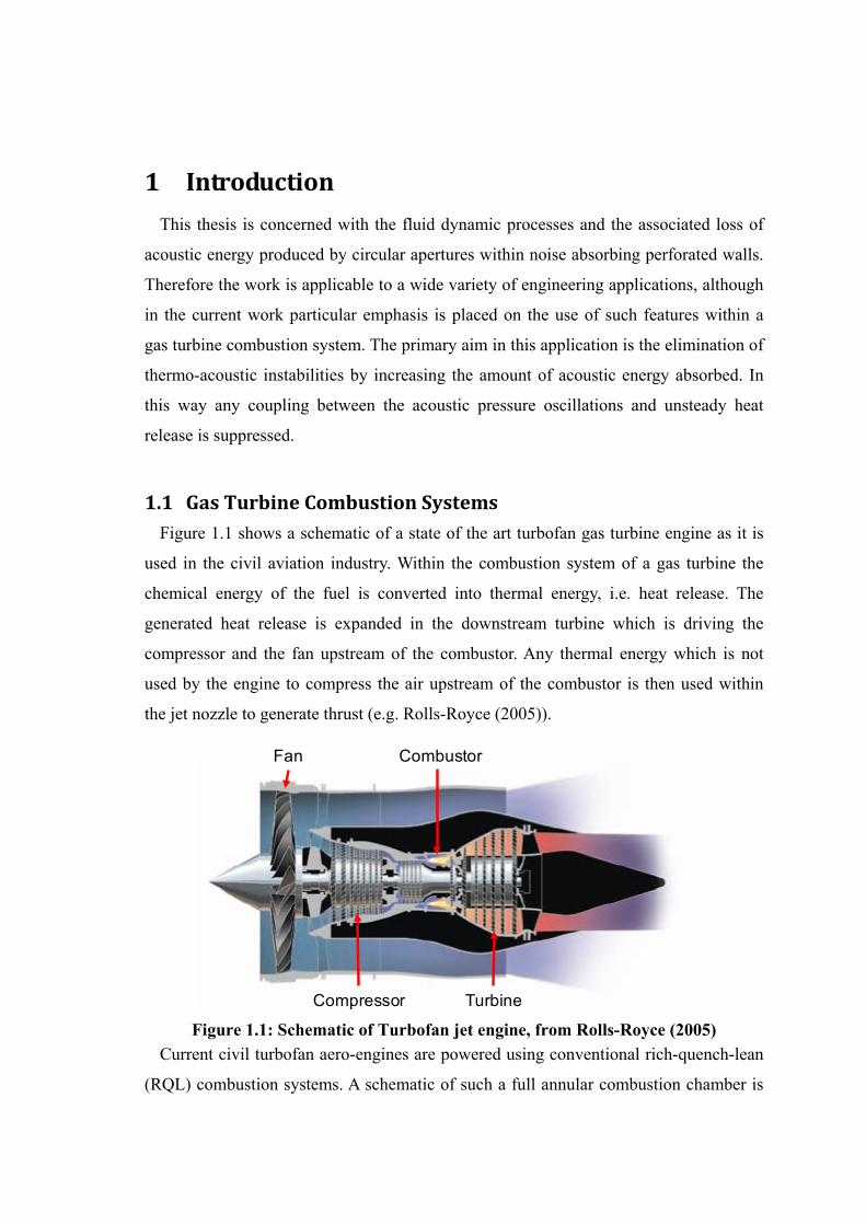
1.1 Gas Turbine Combustion Systems Figure 1.1 shows a schematic of a state of the art turbofan gas turbine engine as it is
used in the civil aviation industry. Within the combustion system of a gas turbine the
chemical energy of the fuel is converted into thermal energy, i.e. heat release. The
generated heat release is expanded in the downstream turbine which is driving the
compressor and the fan upstream of the combustor. Any thermal energy which is not
used by the engine to compress the air upstream of the combustor is then used within
the jet nozzle to generate thrust (e.g. Rolls-Royce (2005)).
Fan
Compressor Turbine
Combustor
Figure 1.1: Schematic of Turbofan jet engine, from Rolls-Royce (2005)
Current civil turbofan aero-engines are powered using conventional rich-quench-lean
(RQL) combustion systems. A schematic of such a full annular combustion chamber is

Introduction 2
shown in Figure 1.2. A more detailed summary of gas turbine combustion chambers can
be found, for example, in Lefebvre and Ballal (2010). The air delivered by the
compressor typically enters the combustion system through an annular pre-diffuser.
Downstream of the pre-diffuser the air is split into various streams with the majority of
the air being fed around the combustor to the primary and secondary ports, the
combustor wall cooling system and the turbine blade cooling system. In addition a small
amount of air enters the combustion chamber via the swirlers of the fuel injector. Thus
the flame is swirl stabilised within the primary zone of the combustion chamber, where
the fuel is atomised, vaporised and mixed with the various air streams prior to
combustion. The aim is to generate adequate residence time and turbulence levels to
generate the required mixing of fuel and air for flame stabilisation.
Figure 1.2: Schematic of conventional gas turbine combustion system (Rolls-Royce
(2005)) The primary and secondary ports are designed to control pollutant emissions by
feeding an optimised amount of air into the combustor. Within the dilution zone the
temperature of the hot gas inside the combustor is further reduced by feeding a further
20-40% of the air into the dilution ports (Lefebvre and Ballal (2010)). The aim of this

Introduction 3
zone is to generate an adequate temperature exit profile which is suitable for the nozzle
guide vane of the high pressure turbine at the exit of the combustor. This is important
for the turbine life and its cooling requirement. Moreover, the radial and overall
temperature profiles at the combustor exit have a significant impact upon the efficiency
of the turbine downstream of the combustor.
1.1.1 Environmental Aspects of Gas Turbine Combustion Systems Pollutant emissions emitted by aviation affect the local air quality near the airports as
well as the upper troposphere and lower stratosphere (8-12 km altitude) for civil
aviation. The pollutant emissions at altitude can cause chemical reactions which lead to
ozone (O3) production and cloud formation. A measure of the affects of the pollutant
emissions on the climate is indicated by the radiative forcing (RF) parameter as
described by Prather et. al. (1999). The radiative forcing index is based on the balance
between radiative heating effects produced by the sun and terrestrial cooling effects.
Any man made emissions in the atmosphere will change this balance and therefore
produce positive radiative forcing (i.e. heating of the atmosphere) or negative radiative
forcing (i.e. cooling of the atmosphere) which will ultimately lead to climate change.
The main emissions emitted by gas turbine combustion systems burning a hydrocarbon
fuel are (Figure 1.3):
• Carbon monoxide (CO) and carbon dioxide (CO2)
• Nitric oxides (NO) and nitrogen dioxide (NO2), which are grouped together
under the term NOX
• Unburned hydrocarbons (UHC)
• soot
• Water vapour (H2O)
The sulphur (S) indicated in Figure 1.3 is controlled via the sulphur content within the
fuel. The major direct emissions which will be affected by the combustion processes are
CO2 and NOX emissions. Carbon dioxide is a greenhouse gas which will lead to positive
radiative forcing. Moreover CO2 is absorbed by the oceans and leads to an increased
ocean acidification. NOX at cruise altitude (8-13km) is leading to chemical reactions

Introduction 4
where methane (CH4) is reduced and ozone (O3) is increased. Ultimately this also leads
to a positive change in radiative forcing (Prather et. al. (1999), ICAO (2010)).
Figure 1.3: Schematic of aviation emissions and their effects on climate change
from Lee et. al. (2009) Currently the impact on CO2 emissions emitted by aviation is 2% of the world total
CO2 emissions (Prather et. al. (1999), ICAO (2010)). However current predictions show
that the world wide air traffic is anticipated to grow by 4-5% per year (ACARE (2011)).
Therefore CO2 emissions will increase if the technology of the used aircraft and engine
is not improved. The Advisory Council for Aeronautics Research in Europe (ACARE
(2001)) set a target to reduce CO2 emissions from aircraft by 50% in the year 2020. For
aero-engine manufacturers this means future aero-engines will have reduced fuel burn
and therefore reduced CO2 emissions in the year 2020 by 15-20% (Rolls-Royce (2010))
as indicated in Figure 1.4. The remaining 20-25% is due to more efficient aircraft and 5-
10% is due to improved air traffic management.

Introduction 5
Figure 1.4: CO2 reduction of Rolls-Royce aero-engines, from Rolls-Royce (2010) The ACARE 2020 target for NOX emissions reductions were set to 80%. On an
engine level this means a NOX reduction in the order of 60% as shown in Figure 1.5. In
this case the NOX reduction is shown relative to a baseline NOX standard given by the
Committee on Aviation Environmental Protection (CAEP) in 2004. More recently
ACARE Vision 2050 (ACARE (2011)) has proposed the CO2 and NOX emissions
targets for the year 2050. In this report a 75% reduction in CO2 and a 90% reduction in
NOX emissions is set. Current aero-engine combustion systems have combustion
efficiencies higher than 99.9% at take-off and cruise conditions (Lewis et. al. (1999),
Rolls-Royce (2005), Lefebvre and Ballal (2010)). The CO2 emissions are directly linked
to the necessary fuel burn, as it is a product of complete combustion. Therefore CO2 can
only be reduced if less fuel is needed for the transport of goods and passengers within
an aircraft. Thus the CO2 emissions are a product of aero-engine efficiency, air frame
efficiency and air traffic management.
Improvements in aero-engine efficiency can be achieved by improving the efficiency
of the components of the engine, i.e. turbomachinery efficiency, leakage reduction,
cooling reductions, etc. Moreover improvements in thermal efficiency can be used to
reduce the amount of fuel used, and thus reduce the amount of CO2 produced, for the
generation of the necessary thrust of the engine. The improvement in thermal efficiency
is achieved by increasing the overall pressure ratio (OPR) of the engine. Unfortunately
this means the combustor inlet temperatures increase, which in turn generates higher
combustion temperatures and thus higher turbine inlet temperatures. Lefebvre and

Introduction 6
Ballal (2010) as well as Lewis et. al. (1999) show that NOX emissions increase with
increasing temperature. Another driver for NOX is the residence time within the
combustor (Lefebvre and Ballal (2010)). Thus improvements in thermal efficiency of
the gas turbine also lead to increasing NOX emissions. Hence different combustion
concepts are necessary to achieve both requirements: reduced CO2 and reduced NOX
emissions.
Figure 1.5: NOX reduction of Rolls-Royce aero-engines, from Rolls-Royce (2010) Current combustion technology utilises RQL concepts to control the NOX emissions
generated in the combustion chamber. As already mentioned nitrogen oxide emissions
are generated at high combustion temperatures which occur near stoichiometric
equivalence ratios (~1). Hence a rapid quenching is needed from rich equivalence ratios
in the primary zone to lean equivalence ratios in the dilution zone leading to reduced
NOX generation as indicated in Figure 1.6. However due to high temperatures in the
primary zone dissociation processes can lead to large amounts of carbon monoxide
(CO). Hence if the mixture is cooled too quickly then the CO would not react any
further which leads to low combustion efficiency and large amounts of toxic CO
emissions.

Introduction 7
Figure 1.6: NOX formation in RQL Combustors, from Lefebvre and Ballal (2010) The drive to low emissions in the future is forcing a change in combustor technology
for aero gas turbines from rich burn to lean burn combustors. In this case the NOX-
increase due to the change from rich (i.e. equivalence ratio larger than one) to lean (i.e.
equivalence ratio smaller than one) air fuel ratio will be avoided and the combustion
process will be undertaken at entirely lean equivalence ratios (equivalence ratios smaller
one in Figure 1.6). Lean premixed prevapourised gas turbine combustors have been
used for industrial machines to achieve the stringent NOX emission targets for land
based gas turbines. Many examples of industrial lean burn combustors can be found in
Huang and Yang (2009). Initial lean burn combustor design for flight engines were so
called double annular combustion systems (Figure 1.7) as shown for example in Dodds
(2002), similar combustion systems can also be found in Lewis et. al. (1999). The
combustor consists of a fuel rich pilot stage (which is always operational) and a lean
mains fuel injector which is optimised for low NOX emissions at high power engine
operation. More recently Dodds (2005) and Klinger et. al. (2008) show a staged lean
burn combustion system where the pilot and mains fuel injectors are combined into one
injector (Figure 1.8). It can be seen that the fuel injectors are much larger than for the
rich burn example. This is caused by the increasing amount of air that is required to
enter the combustor through the fuel injector for lean combustion, which must be
achieved without increasing the combustor pressure drop. For lean burn applications
approximately 70% of the air within the combustor enters through the swirlers within
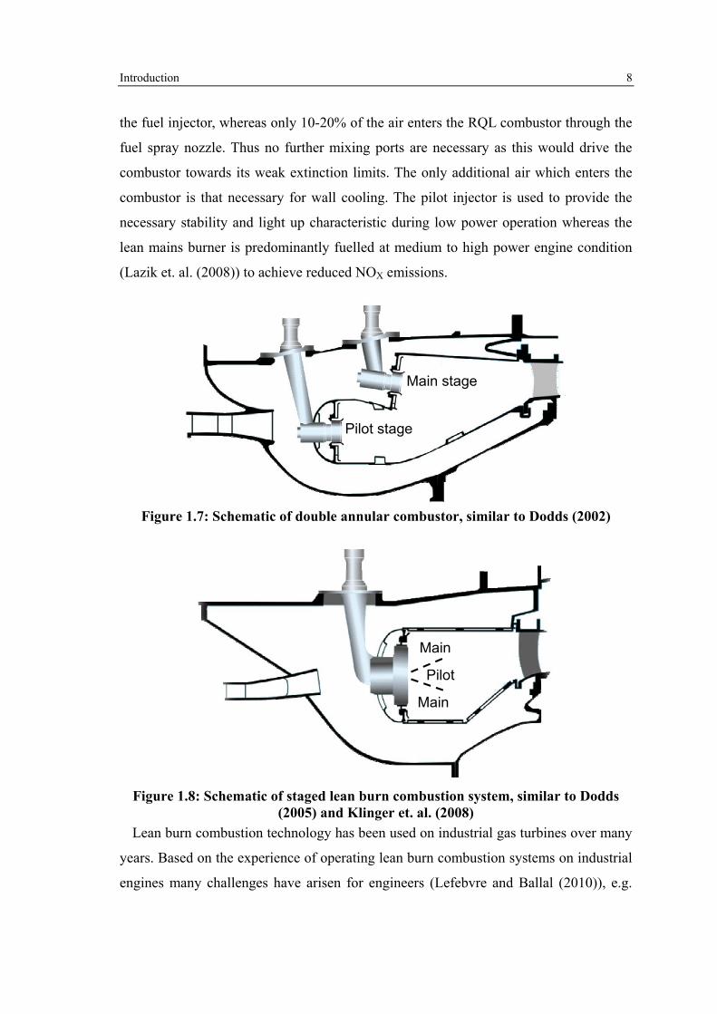
Introduction 8
the fuel injector, whereas only 10-20% of the air enters the RQL combustor through the
fuel spray nozzle. Thus no further mixing ports are necessary as this would drive the
combustor towards its weak extinction limits. The only additional air which enters the
combustor is that necessary for wall cooling. The pilot injector is used to provide the
necessary stability and light up characteristic during low power operation whereas the
lean mains burner is predominantly fuelled at medium to high power engine condition
(Lazik et. al. (2008)) to achieve reduced NOX emissions.
Pilot stage
Main stage
Figure 1.7: Schematic of double annular combustor, similar to Dodds (2002)
Pilot
Main
Main
Figure 1.8: Schematic of staged lean burn combustion system, similar to Dodds
(2005) and Klinger et. al. (2008) Lean burn combustion technology has been used on industrial gas turbines over many
years. Based on the experience of operating lean burn combustion systems on industrial
engines many challenges have arisen for engineers (Lefebvre and Ballal (2010)), e.g.

Introduction 9
flash back, margin to lean blowout, adequate combustion efficiency during operating
envelope, homogeneous air fuel ratio at the fuel injector to achieve low emissions,
sufficiently low pressure loss across the combustion system, etc. For aero-engines there
is also a further challenge which is altitude relight. However, one of the major
challenges for lean burn combustion is the avoidance of thermo-acoustic instabilities,
based on the experience from lean burn combustors operating within industrial gas
turbines. Thermo-acoustic instabilities cause large acoustic pressure oscillations within
the combustor leading to reduced life and possible structural damage. The avoidance of
this instability by increasing the acoustic energy absorption of the combustion system is
the main focus of this thesis.
1.2 Thermo-Acoustic Instability Thermo-acoustic instabilities, also known as combustion instabilities, can occur in
any engineering application where heat is added within a confined volume, such as for
example boilers, furnaces (Putnam (1971)), rocket engines (Hart and McClure (1965),
Yang and Anderson (1995), Culick (2006)), gas turbine combustors (Scarinci and
Halpin (2000), Dowling and Stow (2003), Eckstein (2004), Kaufmann et. al. (2008)),
ramjets and afterburners (Rogers and Marble (1956), Bonnell et. al. (1971), Langhorne
(1988)). Each of those combustion systems is characterised by various acoustic
resonance frequencies due to their geometry. The added heat release rate can couple
with the acoustics of the combustion system geometry, thereby supplying energy to the
acoustic pressure oscillation. This leads to rapidly rising pressure amplitudes within the
combustion chamber due to the large amount of energy being released. The high
pressure amplitudes limit the component life, or in the worst cases, cause structural
damage to the combustion chamber.
In the literature early references to this phenomenon can be found in conjunction with
the singing flame by Higgins (1802), who experimented with hydrogen flames within a
vertical tube generating an audible sound at the fundamental frequency of the tube. A
similar observation was made in conjunction with the well-known Rijke tube. Rijke
(1859) discovered that a loud tone was audible by putting a heated mesh into the lower
half of a glass tube where both ends of the tube were open to atmosphere. Observations

Introduction 10
stated that it was dependent on the position of the heat source if a loud tone was audible
or not. Rayleigh (1896) investigated these phenomena and came to the conclusion that
the added heat release from the mesh is increasing the pressure amplitude associated
with the acoustic resonance mode of the tube. Moreover the heat source has to be placed
so that the added heat release is in phase with the pressure oscillation for the audible
tone to occur. This is the basis of the Rayleigh Criterion for which a simple
mathematical description can be written as (e.g. Lieuwen(1999)):
( ) ( )∫ ∫ ≥⋅V T
lossesacousticdVdttxptxQ ,',' ( 1.1)
If unsteady heat release Q’ is added in phase with the fluctuations in pressure p’ then
the pressure amplitude can potentially increase, whereas if the heat release is added out
of phase with the pressure oscillations then the amplitudes will decay within one time
period T. However, for acoustic pressure amplitudes to grow in magnitude, the product
of unsteady heat release and pressure oscillations has to be larger than the acoustic
losses within the combustion system. This criterion has been used by many authors to
investigate and predict the stability of combustion systems (e.g. Chu (1965), Lieuwen
(1999), Lawn (2000), Dowling and Hubbard (2000), etc.).
In the context of thermo-acoustic instabilities within gas turbine combustion systems
the added heat release by the flame can couple with the acoustics of the combustion
chamber geometry. For example unsteady heat release results in the propagation of
acoustic waves, which can alter the pressure drop across the fuel injector which in turn
causes the velocity field of the fuel injector to oscillate. This can lead to fluctuations in
stoichiometry so that the interaction of the pressure wave with the fuel injector flow
field leads to further unsteady heat release. This simplified feedback mechanism can
thereby lead to self-excitation as shown schematically in Figure 1.9. However the initial
mechanism which is causing the self-excited combustion instability can be much more
complex. More detailed feedback mechanisms can be found in Paschereit e. al. (1999),
Candel (2002) or Sattelmayer (2003). Turbulence and large scale coherent structures
within the fuel injector flow field (Coats (1996), Poinsot et. al. (1987)), local
equivalence ratio oscillations and spatial heat release distribution (Lieuwen and Zinn
(1998), Kato et. al. (2005)) as well as propagating entropy waves within the combustion

Introduction 11
system (Eckstein et. al. (2004), Eckstein (2004)) can cause the onset of thermo-acoustic
instabilities. In general lean burn combustion is more prone to thermo-acoustic
instabilities. One of the reasons for this behaviour is that the changes in rate of
combustion due to oscillations in fuel air ratio is larger for lean combustion than for rich
combustion, especially near the lean blow out regime (e.g. Dowling (2003) or Huang
and Yang (2009)).
Unsteady heat release
Pressure oscillations
Air and fuel mass flow oscillations
Figure 1.9: Thermo-acoustic feedback cycle as in Lieuwen (1999)
The challenge for gas turbine combustion engineers is to develop a lean burn
combustion system design which is not susceptible to thermo-acoustic instabilities.
Ideally the instability needs to be avoided at source, i.e. the design of the fuel injector
suppresses the onset of thermo-acoustic instabilities. Steele et. al. (2000), for example,
reduced the onset of thermo-acoustic oscillations by influencing the residence time of
the air and fuel mixture within the premixing ducts. Further examples of fuel injector
design to effectively avoid combustion instability can be found in Huang and Yang
(2009). However, currently only limited design rules exist to develop a combustion
system fulfilling all the requirements for an aero-engine combustor (Lefebvre and Ballal
(2010)) which then exhibits no susceptibility to thermo-acoustic instabilities over the
operating envelope of the engine. In recent years numerical and experimental studies
have been undertaken to understand the thermo-acoustic characteristic of lean burn fuel
injectors which includes, for example, measurements of flame transfer functions
(Paschereit et. al. (2002), Schuermans et. al. (2010)). The flame transfer function treats
the burner and the flame as a black box and relates the heat release oscillations to the

Introduction 12
input pressure oscillation onto the fuel injectors. If the transfer function is measured in
an acoustic resonance free system, it can be transferred into acoustic models of full
engine combustion system geometry. Hence the stability of the gas turbine combustion
system can then be analysed. With this in mind the described mechanisms can be
investigated and the stability of the gas turbine combustion system can be assessed.
However, as already mentioned, currently there are only limited design rules which can
be used to influence the transfer function of a fuel injector so that there is no risk of
thermo-acoustic instability throughout the operating envelope of an aero-gas turbine
engine. Hence additional forms of the suppression of thermo-acoustic instability are
under development.
One method of control is to influence the phase of the heat release relative to the
pressure oscillation using fuel staging. As already explained in an earlier section staged
lean burn combustion systems can have multiple fuel lines. Therefore the fuel split
between the various injectors can be adjusted so that pressure amplitudes due to thermo-
acoustic instabilities are minimised (Steele et. al. (2000), Scarinci and Halpin (2000),
Mongia et. al. (2003)). This can be achieved by radially and circumferentially staging
the fuel within a fully annular combustion system. The circumferential fuel variation is
also known as asymmetric fuelling. However, due to the changes in combustion
temperatures across the combustor it is possible that stringent NOX emissions cannot be
met using this strategy. Moreover the changes in fuel staging and asymmetric fuelling
can have adverse effects on the temperature profile at combustor exit. This can then lead
to reduced turbomachinery efficiency and a reduced life of the turbine components.
A further option to change the phase relationship between unsteady heat release and
the acoustic pressure oscillation is active control. For example, a dynamic pressure
sensor within the combustion chamber can be used to monitor the acoustic pressure
oscillations. If the pressure amplitudes rise an actuator in the fuel supply line can be
used to oscillate the fuel at the same frequency so that the heat release and pressure
oscillations are out of phase with each other. Many researchers have worked in this field
to develop algorithms for active instability control systems, e.g. Schuermans (2003),
Riley et. al.(2003), Dowling and Morgans (2005), Illingworth and Morgans (2010). All
of this work has shown that it is possible to suppress thermo-acoustic instability by

Introduction 13
controlling the fuel supply. However, most of the work was aimed at stationary gas
turbines operating with gaseous fuels, with the weight and size of the fuel actuators
meaning it is currently not practical for aero-gas turbines. Moreover the challenge
remains to design reliable liquid fuel actuator valves which operate in the range of
several hundred Hertz with a specified accuracy on the fuel modulation amplitudes
within the harsh gas turbine combustion system environment. Moran et. al. (2001)
shows the application of active control on an afterburner of a RB199 full scale military
turbofan aero engine. The tests were conducted on the ground with the active control
being aimed at the low frequency combustion instability known as reheat buzz with
frequencies well below 300 Hz. The system demonstrated a significant reduction in
pressure amplitude and showed the potential for active control applications in the future.
Furthermore Umeh et. al. (2007) studied the use of active control for a gas turbine aero
engine. To overcome the challenge of operating an actuator valve at more than 500 Hz,
the control algorithm was aimed at low frequencies corresponding to half of the
combustion instability frequency. It could be shown that the thermo-acoustic instability
frequency could be successfully reduced by this technique.
All the discussed methods in this section so far have focussed on influencing the
product of the unsteady heat release and the unsteady pressure fluctuation, i.e. the
amount of energy driving the instability. However this work is aimed at the absorption
of the energy, i.e. the optimisation of acoustic losses within a gas turbine combustor. If
the energy absorbed can exceed the amount of energy driving the instability the thermo-
acoustic oscillation can be avoided. In general this is known as the passive control of
combustion instabilities and is presented in the next section.
1.3 Passive Control of Thermo-Acoustic Instabilities Thermo-acoustic instabilities can be passively controlled by increasing the absorption
(i.e. damping) of the acoustic waves within the combustion chamber. Hence, the aim of
this approach is to enhance the acoustic energy absorption within the combustion
system geometry to a level whereby the acoustic pressure amplitudes can be reduced or,
more desirably, the onset of the combustion instability suppressed. The suppression of
the combustion instability is possible if all the generated acoustic energy is absorbed

Introduction 14
before the reflected pressure waves can interact with the fuel injector flow field and
other features of the combustion system. In this case the simplified feedback cycle in
Figure 1.9 can be broken leading to suppression of thermo-acoustic instability. A
modern combustion system contains a variety of components that can potentially
provide some acoustic damping (Figure 1.10). These include, for example, combustor
ports, cooling rings or effusion cooled liners.
Primary and secondary ports
Cooling air
Cooling ring
Or alternatively
Effusion cooling
Cooling air
Figure 1.10: Schematics of common combustor apertures which interact with
acoustic pressure waves In general the amount of damping provided by the various combustor apertures is
assumed to be small, hence the amount of damping is often assumed to be negligible.
Thus additional passive damping devices must be incorporated within the system whose
primary purpose is to absorb acoustic energy. The most common devices used are
Helmholtz resonators and perforated liners.
1.3.1 Helmholtz Resonators
1.3.1.1 The Harmonic Oscillator A Helmholtz resonator, as shown on the left hand side in Figure 1.11 and described
for example in Rayleigh (1896) or Kinsler et. al. (1999), consists of a neck with length L
and cross-sectional area A. One side of the neck is connected to a volume V and the

Introduction 15
other side is open to an incident oscillating pressure amplitude onto the neck. The
Helmholtz resonator is an harmonic oscillator which can be described in its simplest
form as a mass-spring-damper system (right hand side in Figure 1.11). Thus the damped
forced harmonic oscillator can be described using the following differential equation
(Kinsler et. al. (1999):
( ) ( )tiFtFxcdtdx
Rdt
xdm sZ Rexp==++2
2
( 1.2)
This equation describes the balance of forces surrounding the mass element in Figure
1.11), where the parameter x denotes the displacement of the mass. Hence the first term
of the left hand side describes the inertial force due to the acceleration of the mass, the
force due to the resistance RZ within the damper element is given in the second term on
the left hand side and the force due to the spring element is represented in the last term
on the left hand side of equation ( 1.2). The system is forced by a harmonic force which
is equivalent to a pressure oscillation incident onto the neck of the resonator
( ) ( )tipAtF Rexpˆ= , ( 1.3)
where the pressure amplitude is represented by the parameter p . If the wavelength λ is
much larger than the neck length L (λ >> L) the air within the neck can be described as
a single column of air representing the mass m (e.g. Kinsler et. al. (1999)):
effALm ρ= ( 1.4)
As the equation shows the mass is the product of the density ρ, the neck cross-sectional
area A and the effective length Leff. The effective acoustic neck Leff represents the
geometric length L of the neck and an additional acoustic length correction. Acoustic
radiation effects at the neck outlet acts as an additional mass to the neck and are
accounted for by this additional length correction. The end corrections can be estimated
for flanged and unflanged terminations as in Kinsler et. al. (1999):
Flanged termination RLLeff 8502 .⋅+= , ( 1.5)
Unflanged termination: ( ) RLLeff 60850 .. ++= , ( 1.6)

Introduction 16
where R denotes the radius of the neck. In practice these length corrections are often
estimated from experimental data for a given resonator neck geometry.
V
A
L
m
RZ
cs
F(t)
Figure 1.11: Schematic of a Helmholtz resonator and its equivalent harmonic oscil-lator (Kinsler et. al. (1999))
The pressure oscillation within the volume V is assumed to be uniform, in other words
the acoustic pressure amplitude at a given time t is constant throughout the volume.
Moreover the volume V of the resonator represents the spring cS element in the
harmonic oscillator system (third term on the left hand side in equation ( 1.2)). A force is
required to move the mass against the stiffness of the spring which is the product of the
stiffness and its displacement x:
xcF s ⋅= ( 1.7)
For the resonator the stiffness can be estimated by investigating the change of its
volume due to the displacement of the column of air within the neck. In other words it
can be assumed that the air within the neck acts like a piston which changes the volume
by the amount of its displacement and the neck cross-sectional area. If the piston is
pushing into the volume the change in volume can be defined as AxdV −= . As the
volume changes so does the density of the air within the volume:
VAx
VdVd
=−=ρρ , ( 1.8)
therefore the pressure within the resonator volume has to rise, which can be estimated
assuming an isentropic compression:

Introduction 17
xVAcdcp 22 ρ
ρρρ == . ( 1.9)
Parameter c refers to the speed of sound in this expression. The force which is required
to achieve the neck displacement is the force due to the incidental pressure amplitude as
described in ( 1.3). Thus substituting equation ( 1.3) into ( 1.9) and comparing it to
equation ( 1.7) results in a spring stiffness cS of
VA
ccs
22ρ= . ( 1.10)
An important parameter is the impedance Z of the Helmholtz resonator which
describes the relationship between unsteady pressure amplitude incident onto the
resonator neck and unsteady velocity amplitude of the column of air within the neck.
This parameter can be derived using equation ( 1.2) together with equations ( 1.3), ( 1.4)
and ( 1.10):
( )tiApdtuV
AcuR
dtdu
AL Zeff Rρρ expˆ'''
=++ ∫2
2 . ( 1.11)
Note the circumflex above the pressure parameter indicates the amplitude of the
acoustic pressure oscillation. Moreover, in this case the displacement of the mass within
the neck has been expressed as the oscillating velocity which is defined as
( )tiuu Rexpˆ' = . Thus substituting the expression for the oscillating velocity into
equation ( 1.11) leads to the impedance of the Helmholtz resonator
−+=+==
VAcLi
AR
iXRupZ eff
ZZZ R
ρρR2
ˆˆ
, ( 1.12)
where 1−=i . It can be seen that the impedance of the resonator is split into two
parts: the resistance RZ and the reactance of the resonator XZ. The resistance term
influences the amount of acoustic energy being absorbed. The reactance term of the
Helmholtz resonator is equal to zero for the Helmholtz resonator when forced at its
resonant frequency
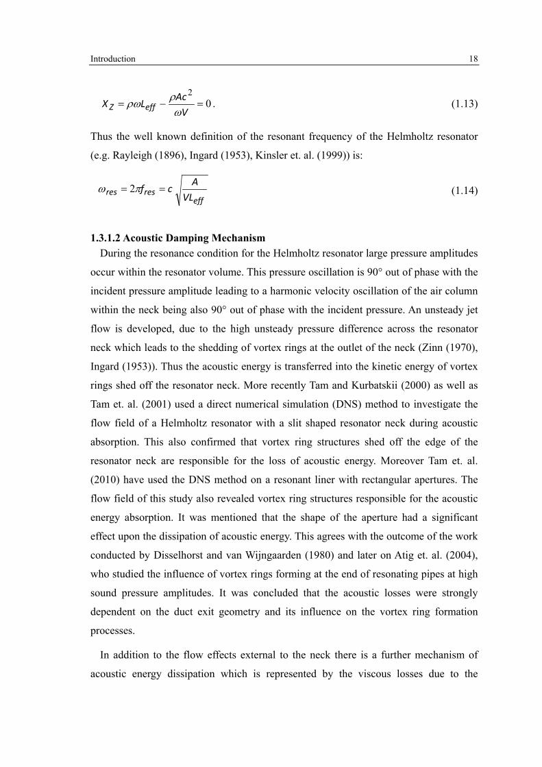
Introduction 18
02
=−=V
AcLX effZ RρρR . ( 1.13)
Thus the well known definition of the resonant frequency of the Helmholtz resonator
(e.g. Rayleigh (1896), Ingard (1953), Kinsler et. al. (1999)) is:
effresres VL
Acf == πR 2 ( 1.14)
1.3.1.2 Acoustic Damping Mechanism During the resonance condition for the Helmholtz resonator large pressure amplitudes
occur within the resonator volume. This pressure oscillation is 90° out of phase with the
incident pressure amplitude leading to a harmonic velocity oscillation of the air column
within the neck being also 90° out of phase with the incident pressure. An unsteady jet
flow is developed, due to the high unsteady pressure difference across the resonator
neck which leads to the shedding of vortex rings at the outlet of the neck (Zinn (1970),
Ingard (1953)). Thus the acoustic energy is transferred into the kinetic energy of vortex
rings shed off the resonator neck. More recently Tam and Kurbatskii (2000) as well as
Tam et. al. (2001) used a direct numerical simulation (DNS) method to investigate the
flow field of a Helmholtz resonator with a slit shaped resonator neck during acoustic
absorption. This also confirmed that vortex ring structures shed off the edge of the
resonator neck are responsible for the loss of acoustic energy. Moreover Tam et. al.
(2010) have used the DNS method on a resonant liner with rectangular apertures. The
flow field of this study also revealed vortex ring structures responsible for the acoustic
energy absorption. It was mentioned that the shape of the aperture had a significant
effect upon the dissipation of acoustic energy. This agrees with the outcome of the work
conducted by Disselhorst and van Wijngaarden (1980) and later on Atig et. al. (2004),
who studied the influence of vortex rings forming at the end of resonating pipes at high
sound pressure amplitudes. It was concluded that the acoustic losses were strongly
dependent on the duct exit geometry and its influence on the vortex ring formation
processes.
In addition to the flow effects external to the neck there is a further mechanism of
acoustic energy dissipation which is represented by the viscous losses due to the

Introduction 19
boundary layer within the neck (Keller and Zauner (1995) or Bellucci et. al. (2004)).
Zinn (1970) as well as Hersh and Rogers (1976) mention that the viscous losses due to
the boundary layer within the neck remain constant with pressure amplitude but the
losses due to the momentum transfer into vortex rings are pressure amplitude dependent
and dominate the acoustic energy absorption at high pressure amplitudes. Hence the
viscosity effects could reduce the acoustic absorption as it reduces the unsteady velocity
amplitudes within the neck and thus the transfer of acoustic energy into vortex rings. All
the described acoustic energy absorption effects, i.e. flow structures external to the neck
and boundary layers within the neck, are accounted by the resistance parameter RR in
equations ( 1.2) or ( 1.12).
If the pressure waves are exciting the resonator away from its resonance frequency
than the pressure fluctuation in the volume is reduced, relative to the resonance
condition, as less power is transferred from the incidental wave into the resonator
volume. This leads to small velocity oscillations and therefore to reduced acoustic
energy loss due to the reduced kinetic energy transfer. Hence the acoustic absorption of
such a device is only adequate over a narrow frequency band close to the resonance
frequency. Therefore the device has to be carefully tuned onto the damping frequency.
1.3.1.3 Non-Linear Absorption of Helmholtz Resonators In general the amount of acoustic energy absorption can be described using an
absorption coefficient. This parameter relates the acoustic energy loss relative to the
incident acoustic energy onto the absorbing device. For a linear acoustic absorber the
absorption coefficient remains constant, i.e. the amount of acoustic absorption is a linear
function of the incident acoustic energy. However, the acoustic absorption characteristic
of a Helmholtz resonator is known to be non-linear. This means that the acoustic
absorption is a function of the incident acoustic pressure amplitude. In other words the
amount of acoustic energy loss generated by the resonator is not increasing or
decreasing at the same rate as the incident acoustic energy. The reason for this
behaviour is the non-linear relationship between the incident pressure amplitude and the
neck velocity amplitude. Ingard and Ising (1967) conducted hot-wire anemometer
measurements at the exit of orifice geometries subjected to various levels of acoustic
pressure amplitudes. It can be seen that for increasing pressure amplitude the orifice

Introduction 20
velocity amplitude was a non-linear function of incident pressure amplitude: 2'~' up .
Moreover it was also noticed that the velocity amplitudes showed the occurrence of
harmonics at large acoustic pressure amplitude forcing.
Due to this non-linear behaviour the acoustic loss generated by the Helmholtz
resonator decreases with increasing incident pressure amplitude (Zinn (1970)). For a
linear acoustic absorber the amount of acoustic energy loss generated is linearly related
to the incident pressure wave, i. e. '~' up (Hersh and Rogers (1976), Ingard and Ising
(1967)). Hence for a linear absorber the relative amount of acoustic energy absorbed to
the incident energy is constant.
1.3.1.4 Application to Gas Turbine Combustors Due to their large acoustic energy absorption Helmholtz resonators have been used in
many engineering applications to reduce the amount of acoustic noise. Putnam (1971)
discussed an application of a resonator to a combustion chamber of an aircraft heater
and it was mentioned that the pressure oscillations in the tubular combustor could be
completely suppressed. Laudien et. al. (1995) describes the use of Helmholtz resonators
to successfully reduce the pressure amplitudes within rocket engine combustors.
Bellucci et. al. (2004) and (2005) have shown that the pressure amplitude within an
industrial gas turbine combustor can be greatly reduced by using Helmholtz resonators.
Moreover Gysling et. al. (2000) significantly reduced the pressure amplitudes within a
three sector test rig of a full annular industrial gas turbine combustor. Further
applications of Helmholtz resonators on a can-annular combustion system of an
industrial gas turbine have been reported by Krebs et. al. (2005). It was shown that the
operating envelope of the gas turbine could be increased due to the application of
Helmholtz resonators to the combustor. Scarinci (2005) successfully damped low
frequency pressure oscillations on an aero-derivative industrial gas turbine using
Helmholtz resonators.
One of the challenges of applying a Helmholtz resonator to a gas turbine combustor is
to adequately cool the device. Moreover, due to the large velocity oscillations within the
resonator neck, hot gas from the combustion chamber can be ingested into the resonator
volume (Barker and Carrotte (2006)). Therefore cooling air has been used to

Introduction 21
continuously flush the resonator cavity as shown in Keller and Zauner (1995). The same
technique has been applied in Bellucci et. al. (2004) and (2005) or Krebs et. al. (2005).
Within gas turbine combustion systems the resonators have to be carefully placed.
First of all the resonators can only generate acoustic damping if they are placed where
an oscillating pressure occurs. This is especially important if the resonator is placed
within a combustion system generating acoustic standing waves. In this case regions of
the combustion system are exposed to the maximum acoustic pressure oscillation, i.e.
anti-nodes, and locations at which no pressure oscillations occur, i.e. nodes. Thus
maximum absorption is achieved if the resonator is located at a pressure anti-node. If
the resonator is placed on an acoustic node no acoustic absorption can be generated.
Hence knowledge of the acoustic mode shape within the combustion system is crucial.
Moreover the resonator itself can significantly influence the mode shape within an
acoustic system. Thus pressure nodes can occur within a combustion system at the
resonator position. Hence at least a second resonator is needed, placed half a wave
length away, to be able to damp the acoustic pressure wave. However, due to the
interactions of the resonators with the acoustic waves various other acoustic resonance
modes can occur as shown in Stow and Dowling (2003). Laudien et. al. (1995) also
reported that the distance between the various resonator locations was important to
stabilise the acoustic system within a rocket engine combustor.
Garrison et. al. (1972) investigated the design of Helmholtz resonators for the
application in afterburners. In this case multiple resonators were used to damp the
pressure oscillations occurring in a jet engine afterburner. A perforated plate was used as
shown in Figure 1.12. The volume is enclosed by the perforated plate and the backing
cavity. Each aperture with cross-sectional area Sn is equivalent to one separate
Helmholtz resonator. Therefore each aperture within the perforated liner represents a
resonator neck, with an associated neck length equal to the plate thickness. The volume
of each resonator is defined by the area within one aperture pitch Pa and the
corresponding backing cavity depth S. If the incident wave is normal to the perforated
liner and the amplitude of the incident wave is not changing along the perforated liner,
then no walls within the backing cavity are necessary (as there is no phase difference
between the pressure amplitudes in the several volumes). Nevertheless the volumes can

Introduction 22
be separated, for example with a honeycomb panel, to avoid the onset of any mode
shapes within the backing cavity volume.
V1 V2 V3… Vn
A1 A2 AnIncident sound wave
S
Pa
Figure 1.12: Helmholtz resonator application for jet engine afterburners as used in Garrison et. al. (1972)
Resonator arrays as shown in Figure 1.12 can be also used in jet engine intakes and
exhausts. In these cases the resonator necks can be exposed to high velocity cross-flows
which interact with the acoustic absorption of a resonator. Ko (1972) has investigated
the absorption of a liner with multiple resonators under two different duct flow regimes:
uniform flow and shear flow. The mean flow Mach number was varied between 0 and
0.6. It is shown that the boundary layer thickness has an influence on the sound
attenuation but this is specific to the Mach number, the flow direction and the acoustic
mode within the duct. Cummings (1987) investigated the performance of a resonator
under fully developed turbulent pipe flow for internal combustion engine exhaust
silencers.
1.3.1.5 Review of Acoustic Studies of Helmholtz Resonators Helmholtz resonators can come in a variety of configurations. The geometrical
dependencies of a Helmholtz resonator have been investigated analytically, numerically
and experimentally by many authors. Ingard (1953) has investigated resonators with
circular and rectangular necks connected to circular and rectangular volumes. The focus
of the work was to produce design tools for the various geometries to achieve optimum
sound absorption and to estimate their resonance frequencies. Moreover Selamet and
Lee (2003) investigated resonators with their necks extended into the volume which can
be very useful if design space is limited as, for example, in jet engines. Chanaud (1994)
has developed models to predict the resonance frequencies with various neck cross-

Introduction 23
sectional areas, e.g. cylindrical, rectangular and cross-shaped. Tang (2005) has also
shown that the sound absorption of a Helmholtz resonator can be improved if the neck
of the resonator is tapered. Moreover a model was developed which predicts the
resonance frequency of a Helmholtz resonator with a tapered neck.
Unfortunately, Helmholtz resonators only provide absorption over a relatively narrow
frequency range, i.e. within a narrow band around its resonance frequency, and this
often conflicts with the requirement for adequate acoustic damping throughout the
operating range of the gas turbine. To overcome this issue a range of resonators can be
connected to the combustion system geometry tuned to various frequencies as
mentioned in Richards et. al. (2003). This has also been demonstrated for silencer
systems (e.g. Seo and Kim (2005)). This technique could also be applied to jet engine
intakes and exhaust ducts or afterburners. Garrison et. al. (1972) investigated resonator
geometries in series as shown in Figure 1.13 for their application in jet engine
afterburners. In this case the two resonator frequencies are closely tuned to each other
using the volume sizes or the length, diameter and porosity of the perforations.
Therefore the interaction between the two devices enables large acoustic absorption
over a wider frequency band.
Volume 1
Volume 2
Perforation 1
Perforation 2
Incident pressure amplitude
Figure 1.13: Helmholtz resonators in series similar to Garrison et. al. (1972), or Bothien et. al. (2012)
Similar concepts have been investigated by Bothien et. al. (2012) within industrial gas
turbine combustors. Moreover Hafsteinsson et. al. (2010) showed resonators in series as
a method to suppress fan noise in the intake of a jet engine. Furthermore Xu et. al.
(2010) has developed theoretical models to describe the same concept.

Introduction 24
To overcome the narrow frequency band characteristic Zhao and Morgans (2009)
have used active control in conjunction with a Helmholtz resonator. In this study the
resonator neck area was controlled with an active control system to successfully
suppress the instability of a Rijke tube. A further example of actively tuning a resonator
was also conducted by Zhao et. al. (2009). In this case the back plate of a resonator
volume was vibrated by a control system to actively increase the acoustic absorption of
the resonator over a wider frequency bandwidth. Another option of tuning a resonator
onto the frequency of a combustion system would be to actively change the volume of
the resonator (e.g. De Bedout et. al. (1997)).
1.3.2 Multi-Aperture Perforated Screens with Mean Flow
1.3.2.1 Absorption Mechanism of Circular Holes with Bias Flow Including orifices and ports in combustion chambers can suppress thermo-acoustic
oscillations as described in Putnam (1971). The amount of apertures needed to
significantly reduce the pulsations was evaluated experimentally which is indicated by
the quote in Putnam (1971):
“To stop pulsation, drill one hole in front of the furnace; if that doesn’t work, drill two
holes!”
Initial investigations of the acoustic energy transmission through jet nozzles, e.g.
Bechert et. al. (1977), showed that the loss of acoustic energy was dependent on the
mean bias flow through the nozzle. Bechert (1980) found that the acoustic energy
absorption at low frequency is a function of the mean Mach number through the jet
nozzle. Howe (1979a) also investigated the absorption of sound due to the flow through
a jet nozzle (Figure 1.14) analytically for low Mach numbers by using a vortex sheet
model and described the mechanism with which acoustic energy is absorbed within the
jet flow. A flow with mean jet velocity Uj passing through the orifice develops a
vorticity sheet downstream of the jet nozzle. This vorticity sheet lies in the region of
shear between the core nozzle flow and the surrounding air, with the vortex sheet origin
being at the edge of the nozzle. An incident acoustic pressure wave pi travels towards
the jet nozzle and at the nozzle part of the acoustic energy will be reflected back
upstream (pr), part of the acoustic energy gets transmitted through the nozzle whilst

Introduction 25
some of the acoustic energy is absorbed. Basically the incident pressure oscillation
alters the pressure drop across the jet nozzle which generates a pulsatile jet flow. Thus
the velocity amplitude in the exit of the jet nozzle enhances the shedding of vorticity in
the free shear layer on the edges of the nozzle. The mean flow convects the vorticity
away from the orifice rim and the generated vorticity subsequently is transformed into
heat further downstream via viscous dissipation processes. Therefore acoustic energy is
transferred into kinetic energy associated with the vorticity structures in the shear layer
of the unsteady jet flow.
pi
pr
U
UJ
Shear flow
Figure 1.14: Schematic of a jet nozzle from Howe (1979a)
Howe (1979b) applied a similar theory to develop an analytical model to predict the
acoustic losses associated with a circular orifice subjected to an unsteady pressure drop
with mean flow. In this case Howe (1979b) assumed that the orifice plate is
infinitesimal thin, the jet flow is irrotational and vorticity is similarly shed in a thin
cylindrical shear layer starting from the edge of the aperture. However, the mechanism
related to the acoustic absorption basically remained the same. One outcome of this
work was the development of an analytical expression to describe the Rayleigh
Conductivity for an orifice. The Rayleigh conductivity KD relates the unsteady volume
flow Q through an orifice to the unsteady pressure drop across the orifice
dsus ppp ˆˆˆ −=∆ :
( ) ( )( )StiStDppQiK
dsusD δRρ
−Γ=−
−=ˆˆˆ
( 1.15)

Introduction 26
In this case R represents the angular frequency of the oscillation, D represents the
orifice diameter and the indices us and ds denote the pressure just upstream and
downstream of the orifice. The parameter Γ is a measure of the inertia within the
orifice flow field and the variable δ represents the acoustic admittance of the orifice.
The admittance is a measure of the ability of the orifice velocity flow field to oscillate.
Moreover the amount of acoustic energy being absorbed is proportional to the acoustic
admittance (Howe (1979b), Luong et. al. (2005)). Hence increases in admittance result
in an increasing amount of acoustic absorption.
0
0.1
0.2
0.3
0.4
0.5
0.6
0.7
0.8
0.9
1
0 1 2 3 4 5 6 7 8
KD/D
Strouhal number - St
AdmittanceInertia
Figure 1.15: Rayleigh Conductivity as in Howe (1979b)
For the assumptions made the solution of the model derived by Howe (1979b)
showed that the Conductivity is only dependent on the Strouhal number (Figure 1.15):
DD UR
URf
StRπ
==2
( 1.16)
and is defined using the angular frequency of the pressure oscillation ω, the aperture
radius R and the mean velocity in the plane of the aperture DU .
It can be seen that the ability to absorb acoustic energy (δ ) steadily increases with
Strouhal number in the range 0 < St < 1. After that the ability to absorb acoustic energy

Introduction 27
steadily decreases to an asymptotic value. As described by Howe (1979b) the variation
of admittance (δ), and hence absorption, with Strouhal number is due to the length
scales associated with the vorticity produced by the incident acoustic waves around the
rim of the aperture. At large Strouhal numbers the shed vorticity will have a small
influence on the fluctuating orifice flow. This is because small length scales mean the
induced velocities from individual vortex rings cancel. However, at low Strouhal
numbers the large length scales mean the vorticity of one sign can stretch far
downstream and will impact on the flow through the orifice.
The inertia ( Γ ) is negligible at low Strouhal numbers as the time scales are large for
the oscillating velocity field to react to the pressure oscillation. Hence at Strouhal
numbers close to zero the velocity field in the aperture is in phase with the incident
pressure wave. With increasing Strouhal number the mass of the fluid within the
aperture becomes more significant and the influence of inertia on the fluctuating
velocity amplitude within the orifice increases. Thus the phase between the incident
pressure fluctuation and the velocity oscillation within the aperture increases towards
the high Strouhal number limit ( 1→Γ , 0→δ ). In this case the phase difference
between the incident pressure and the velocity is 90 degrees.
The broadband characteristic of the absorption is mainly due the inclusion of mean
flow through the aperture of the nozzle and its generation of a vorticity sheet. Acoustic
waves over a wide frequency band can interact with the vorticity structures so giving
rise to the broadband characteristic.
1.3.2.2 Perforated Walls with Bias Flow and Linear Acoustic Absorption The acoustic absorption of a perforated wall with bias flow remains in the linear
acoustic absorption regime as long as the unsteady velocity amplitude within the
aperture is smaller than the mean flow velocity through the orifice ( '~' up for Uu <<' ).
In this case the acoustic admittance and inertia of the orifice flow is independent of the
incident excitation pressure amplitude. Moreover the acoustic absorption coefficient
remains constant with increasing pressure amplitude as the acoustic energy loss is
increasing in proportion to the incident acoustic energy. In general, as mentioned in the
previous section, Helmholtz resonators have very little (or no) flow across the neck of

Introduction 28
the resonator. Hence the neck velocity amplitude is larger or similar to the mean
velocity through the neck ( 2'~' up for Uu ≥' ). Therefore the absorption is within the
non-linear absorption regime. Hence the admittance and inertia are a function of
incident pressure amplitude and the acoustic absorption coefficient changes with
increasing incident pressure amplitude.
Many investigations into the absorption of perforated liners either within the linear
absorption regime (e.g. Hughes and Dowling (1990), Jing and Sun (1999), Eldredge and
Dowling (2003), Lahiri et. al. (2011), etc) or in the non-linear absorption regime (e.g.
Salikuddin and Brown (1990), Salikuddin et. al. (1994) or Cummings (1986), etc) have
been described. Only a few researchers have investigated the transition from linear to
non-linear absorption (Ingard and Ising (1967), Melling (1973), Betts (2000) Bellucci
et. al. (2004b).
As already mentioned the point at which the transition between linear and non-linear
absorption occurs is dependent on the velocity amplitude relative to the mean velocity.
Therefore the flow field generated by the acoustic pressure amplitude and its
dependency on the orifice geometry needs to be further understood. Hence there is a
need for detailed flow field studies on the transition from linear to non-linear absorption
for gas turbine combustor relevant orifice geometries and absorption regimes over the
operating range of a gas turbine combustion system.
1.3.2.3 Application to Gas turbine Combustors Due to the ability of absorbing adequate amounts of acoustic energy over a broad
frequency bandwidth acoustic liners with mean bias flow have also been applied to gas
turbine combustors. Scarinci (2005) showed the application of an acoustic liner within
an aero-derivative Rolls-Royce Trent 60 industrial gas turbine. Moreover a similar type
of damper has been introduced by Lörstad et. al. (2009) in a SIEMENS SGT 800
industrial gas turbine combustor. It has been shown that the pressure amplitudes within
the combustion system could be significantly reduced compared to the previous design
without the perforated wall. Macquisten et. al. (2006) used a porous liner within a
tubular single sector combustion rig with a down-scaled industrial gas turbine burner.
The instabilities generated by the burner could be suppressed successfully if the mean

Introduction 29
flow across the porous liner was sufficiently low. Perforated liners backed by a resonant
cavity have also been used successfully by Tran et. al. (2008) to control the inlet
boundary condition of a gas burner. Perforated liners to reduce the noise generated by a
jet engine fan have also been used within the intake of jet engines (Dean and Tester
(1975), Betts (2000)).
1.3.2.4 Review of Acoustic Experiments on Perforated Liners Many studies into the bulk absorption characteristics of perforated liners have been
undertaken to optimise the absorption of the liner geometry and understand the relevant
design parameters. Perforated liners backed by a resonant cavity have been investigated
for example by Hughes and Dowling (1990). In this investigation a perforated liner
backed by a rigid wall, as shown in Figure 1.12, has been studied with a bias flow
across the perforated wall. Note the Helmholtz resonator study introduced in section
1.3.1.4 aimed at the non-linear acoustic absorption regime, where the velocity
oscillation is in the order of the mean flow if not larger ( Uu ≥' ). For the liner backed
by a resonant cavity with mean flow, which is the case in this section, the acoustic
absorption is investigated in the linear acoustic absorption regime. Thus for the purpose
of this study the velocity amplitudes were much smaller than the mean flow velocity,
i.e. Uu <<' . In this case the bias flow represents the cooling flow through the apertures
of a passive damping device applied to a jet engine afterburner. This application is also
known as a screech damper. Screech is a high frequency (more than 1 kHz) thermo-
acoustic instability which occurs in tubular geometries and is characterised by
circumferential or radial pressure waves within the tubular afterburner duct. These
pressure waves can be damped by a perforated liner with resonant backing cavity.
The absorption generated by a perforated liner backed with a plane rigid screen is
frequency dependent. If the system is in resonance it is possible to absorb all incident
acoustic energy for the geometries investigated. Moreover Hughes and Dowling (1990)
also developed an analytical model to describe the acoustic absorption of the tested
liner. The model was based on the theory developed by Howe (1979b) and showed good
agreement with the acoustic measurements. A similar investigation has been undertaken
by Dowling and Hughes (1992) where an array of slits was investigated instead of a

Introduction 30
circular aperture. Again all the incident sound energy could be absorbed if the
perforated liner was backed by a resonant cavity.
Jing and Sun (1999) investigated a similar arrangement as in Hughes and Dowling
(1990). It was shown that the acoustic absorption of a perforated liner backed by a
resonating cavity can be enhanced by introducing a mean bias flow through the
perforation. Moreover, not only was the absorption increased but the frequency band
over which increased acoustic absorption occurs was larger. Jing and Sun (1999)
extended the theory presented in Howe (1979b) by adding an acoustic length correction
to the theory. Comparisons to the measurement showed good agreement. Moreover Jing
and Sun (2000) developed a numerical model of the shear layer downstream of the
orifice by including more realistic orifice jet profiles measured by Rouse and Abul-
Fetouh (1950) for sharp edged apertures. It was intended to model the orifice length
effects more realistically for orifice length-to-diameter ratios ranging from 0.4 to 0.6.
This model showed significant differences to the modified theory developed by Howe
(1979b) and Jing and Sun (1999).
Eldredge and Dowling (2003) applied the length corrected model from Jing and Sun
(1999) based on the theory developed by Howe (1979b) to acoustic absorption
measurements with a grazing flow across the perforated liner. In this case the perforated
liner was backed by a volume which was not in acoustic resonance. The developed
model showed good agreement for the investigated geometries with the absorption
model which does not take the grazing flow effects into account. Forster and Michel
(2003) investigated the absorption of perforated plates with open area ratios from 4 to
20%. It is reported that the absorption of the liners could be increased within a Mach
number range associated with the mean flow across the liner. Heuwinkel et. al. (2007)
investigated experimentally various liners of different porosity at various mean bias
flows and mean grazing flows across the perforated liner. It is shown that more than
50% of the acoustic energy could be absorbed over a wide frequency bandwidth.
Observations of the data showed that the absorption was dependent on the bias flow
velocities. A further observation was made that the absorption of the liner increased
with increasing spacing between the apertures. Furthermore, Lahiri et. al. (2011)
developed an experimental database of the acoustic bulk properties relating to

Introduction 31
perforated liners including variations on bias flow, liner porosity, liner thickness,
grazing flow across the liners as well as the orifice shape. In general the experimental
data agreed with the used acoustic absorption model based on the Conductivity
developed by Howe (1979b).
In general for acoustic absorbers to work, the pressure drop across the perforated liner
has to be sufficiently low. However, for many practical engineering applications and, in
particular gas turbine combustion applications, it is likely that the Strouhal number is
relatively low (Rupp et. al. (2012)). For example in the case of standard effusion
cooling geometries the Strouhal number can be much smaller than 0.1. This is due the
pressure drop distribution of impingement effusion cooling geometries with a total wall
pressure loss typically of order 3% and the typical instability frequencies being below
1000 Hz for large gas turbine jet engine. Hence any reduction in pressure drop to
significantly increase the orifice Strouhal number, and therefore its ability to absorb
acoustic energy (Figure 1.15), leads to significant reductions in cooling performance.
Moreover reduced wall pressure losses lead to a significant increase in the risk of hot
gas ingestion.
Finally the space envelope for a damping device for flight engine gas turbine
combustion systems is limited due to weight constraints. Hence the application of an
optimised broadband linear absorber remains challenging (Rupp et. al. (2012)).
Enhancement of the linear acoustic absorption by using resonant liner applications leads
to the application of large length-to-diameter orifice geometries due to the limited
volume in the combustor design envelope. Hence efficient damping designs have to be
developed which satisfy the damping, cooling and weight requirements for a
combustion chamber of a flying jet engine. Therefore accurate modelling techniques
describing the gas turbine combustion chamber design envelope are necessary and not
fully understood for the investigated geometry and operating conditions within this
study.
1.3.2.5 Numerical Flow Field Investigations Related to Acoustic Absorption for Perforated Liners with Bias Flow
Eldredge et. al. (2007) used a Large Eddy Simulation (LES) model to calculate the
Rayleigh conductivity and compare the results to those of the analytical model proposed

Introduction 32
by Howe (1979b). The analytical conductivity model and the LES calculation compare
reasonably well for the low frequency range. However, it is suggested that the analytical
model needs to be modified for more sophisticated geometries (e.g. angled holes) and
also needs to include the effect of liner thickness. These features can induce shear layers
inside the aperture which give rise to more complicated interactions between the
acoustic energy and unsteady velocity fields. LES velocity contours are presented which
show separated jets introducing shear layers inside the aperture, as well as downstream
of it, which will influence the acoustic energy dissipation. More recently Mendez and
Eldredge (2009) compared the results derived from an LES study with various
analytical absorption models. The LES based data was in good agreement with the more
detailed model presented by Jing and Sun (2000) using jet profiles. Hence the profile of
the jet is also of importance to accurately predict the acoustic absorption of an orifice
plate with varying thickness-to-diameter ratio. Moreover the potential of LES was
shown for understanding the fluid dynamic processes related to acoustic absorption. In a
similar way Andreini et. al. (2011) used LES to investigate the flow fields of perforated
liners. The acoustic absorption calculated by the LES study was compared to the models
developed by Howe (1979b) and Jing and Sun (1999) as well as to the test results from
Bellucci et. al. (2004b). The models did in general agree within the investigated orifice
experiments but also showed differences to the investigated analytical models.
Gunasekaran and McGuirk (2011) developed a pressure based CFD methodology to
adequately captures the acoustic wave propagation in low Mach number (i.e. essentially
incompressible) flows. The predictions were in good agreement with the acoustic
absorption data measured by Rupp et. al. (2010b). Moreover the method presented by
Gunasekaran and McGuirk (2011) showed the same flow field characteristics in the
numerical solutions as highlighted by the PIV measurements from Rupp et. al. (2010b).
Nevertheless the application of CFD to acoustic absorption processes is challenging
since this involves large grid sizes and small time steps. This leads to the calculation of
single apertures. In RANS (Reynolds Averaged Navier Stokes) CFD modelling
techniques the choice of an adequate turbulence model will be important for an accurate
prediction of the unsteady flow flied. Moreover, in LES based approaches, the accuracy
of the employed sub-grid scale models will have an effect on the accuracy of the

Introduction 33
unsteady velocity field prediction. Furthermore there is a lack of measured unsteady
velocity field data in the vicinity of circular apertures during acoustic absorption, which
is of great importance for the validation of the numerical predictions and the analysis of
the found discrepancies between the analytical absorption models and the numerical
solutions derived by CFD.
1.4 Objectives In general this work is aimed on the investigation of the acoustic energy loss
associated with passive damping techniques applied to practical engineering geometries
with the emphasis of gas turbine aero-engine combustion systems. The use of passive
damping techniques was successfully applied to industrial gas turbine combustion
systems. Apart from the application to afterburners, this technology has not been
applied to aero-engine gas turbine combustors. The challenge to design efficient
acoustic absorbers for gas turbine combustors for aero jet engine applications lies within
the compromise between combustor wall cooling demands, sufficiently low bias flow
velocities for achieving adequate acoustic absorption as well as the challenge of fitting a
damper geometry within the limited design space of an aero gas turbine (i.e. to
minimise the impact upon the weight of the engine). The air split through a gas turbine
aero engine combustor is well defined to satisfy the combustion requirements along
with the cooling requirements for the combustor walls and the downstream high
pressure turbine. Moreover in lean burn combustion systems a large amount of air has to
enter the combustor through the fuel injector to achieve the low emission targets.
Furthermore the amount of flow through the damper device incorporated into the
combustor wall could affect the cooling efficiency of the wall and even the combustion
process near the perforated wall. Thus reduced combustion efficiency and increases in
emissions can be expected. Hence the passive damper design can only use a limited
amount of air, to stay within the air budgets of the combustion system and the
downstream high pressure turbine. All the mentioned aspects have to be assessed
throughout the design process of an acoustic damper incorporated into this challenging
environment. Hence further improvements to the currently available design tools are
necessary.

Introduction 34
The main objective of this work is to provide the means by which the acoustic energy
loss associated with a conventional gas turbine combustion system can be determined.
To be able to fulfil the main objective of this work the acoustic characteristics of the
unsteady flow through various apertures typically found in aero engine gas turbine
combustors and their operating conditions need to be investigated. In this case length-
to-diameter ratios between 0.5 and 10 can be typically found for various combustion
system features. Acoustic measurements of various porosities have been conducted in
the past (as discussed in the previous sections) but are often concerned with relatively
thin apertures with small length-to-diameter ratio and do not fully extend over the
operating conditions and geometries found within practical engineering geometries.
Moreover the previously mentioned studies of acoustic dampers are often limited to the
linear acoustic absorption regime. During the occurrence of thermo-acoustic instabilities
it is possible that large pressure amplitudes within the combustor are generated. Hence
not only the linear acoustic abruption regime will be investigated but also the non-linear
acoustic absorption regime. Furthermore many linear acoustic absorption theories aimed
on predicting the acoustic energy loss of apertures are based on the assumption of
infinitesimal thin apertures with cylindrical shear layers. Hence the performance of
these modelling techniques need to be assessed over the geometry range and operating
range of gas turbine combustors. A further objective is the optimisation of the
investigated geometries to enhance the acoustic absorption within a combustion system.
Only limited studies have investigated the influence of the shape of the aperture upon
the linear and non-linear acoustic absorption. Hence better understanding of the aperture
geometry influence is necessary, not only to increase the acoustic absorption available
but also to improve current modelling technologies and extend them to those
geometries.
Many studies in the reviewed literature where concerned with the optimisation of
passive damping systems. However the majority of these cases where aimed on
determining the global acoustic properties of the system, i.e. the acoustic absorption of
the device. Little work has been undertaken to investigate the fluid dynamic processes
leading to acoustic absorption associated with circular apertures. Some of the work,
which has been conducted numerically, has shown that the flow field is of great

Introduction 35
importance for the loss of acoustic energy. This is further illustrated by the observed
changes in acoustic absorption characteristics as the mean flow passing through the
orifice is varied. Hence to understand the acoustic absorption characteristics and the
orifice shape influences further it is necessary to investigate the unsteady fluid dynamic
processes leading to the loss of acoustic energy. Current linear and non-linear acoustic
modelling tools are simulating the unsteady velocity field interaction with the incident
pressure field. A more detailed measurement of the relevant fluid dynamic processes is
necessary to improve the accuracy of the current modelling tools. Therefore a
methodology shall be developed which identifies the relevant fluid dynamic processes
associated with the acoustic energy absorption of circular apertures. The aim for this
work is to assess the unsteady flow field experimentally. However the data can then be
used as validation data for future CFD applications in follow on work.
As already mentioned acoustic dampers applied to gas turbine combustors operate
within a challenging environment where complex swirling flow fields are used to
efficiently atomise and mix the air and fuel prior to combustion. These complex flow
fields have the potential to interact with the unsteady flow field of the circular apertures
within the acoustic damper. The acoustic absorption characteristics described in the
literature are mostly based on simple acoustic ducts, with and without cross-flow
arrangements, and in the absence of more complex swirling flow fields. Thus an
investigation of the influence of such complex flow fields interacting with the acoustic
damper performance needs to be assessed. This will then deliver an understanding if
simplified test rigs to assess the acoustic absorption performance are sufficient.
Finally the gained knowledge from the previously described tasks should be used to
improve the current design tools for acoustic absorbers. This should include an
improvement in the accuracy of the acoustic absorption prediction for various gas
turbine representative orifice geometries with length-to-diameter ratios of 0.5 to 10.
As the acoustic damping geometry in this work will have a cooling flow through the
aperture the focus on the modelling technique will be on the linear acoustic absorption.
This would be sufficient for an accurate stability assessment of a full annular combustor
as initially the amplitudes would remain small. If the combustion system is unstable the
pressure amplitudes will grow and the acoustic absorption transitions into the non-linear

Introduction 36
regime. In this case hot gas can be ingested into the damper cavity which causes the
combustor wall to overheat. Hence the design tool should include the assessment of the
risk of hot gas ingestion to occur and identify the shortfalls in the non-linear acoustic
absorption modelling tools.

Fundamentals of Unsteady Flow through a Circular Orifice 37
2 Fundamentals of Unsteady Flow through a Cir-cular Orifice
This section outlines the fundamental fluid dynamic and acoustic processes for
unsteady jet flow through circular orifices. Initially a brief introduction to jet flows is
given for steady state conditions followed by the concept of vorticity and its link with
the unsteady flow characteristics of round jets. The acoustic governing equations are
also introduced along with the fundamental assumptions associated with the acoustic
modelling techniques for circular apertures.
2.1 Steady State Flows through Circular Orifice Plates On the left hand side of Figure 2.1 a schematic of an orifice located within a steady
(i.e. time independent) total pressure field (P1 and P2) is shown. Fluid is flowing
through the orifice and a jet develops downstream of the aperture (right hand side of
Figure 2.1).
D
Flow direction
P1, p1 P2, p2
D d
Flow direction
Irrotational flow
shear flow
shear flow
vena contracta
Figure 2.1: Schematic of flow through a circular orifice
The flow regions of the jet can be divided into
• An inviscid core flow in the centre of the jet (which is also irrotational)
• A viscous region which corresponds to the shear layer surrounding the
inviscid core of the jet.

Fundamentals of Unsteady Flow through a Circular Orifice 38
In general inviscid flow can be described by continuity of mass (Oertel and Boehle
(2002))
0=∇+∇+∂∂
uut
ρρρ , ( 2.1)
and momentum
0=∇+∇+∂∂ puu
tu
ρρ . ( 2.2)
In this case we assume the flow is incompressible ( const=ρ ) as the Mach number of
the flow is small (M << 1). Moreover the flow is assumed to be steady ( 0t =∂∂ ).
Therefore the momentum equation can be integrated along a stream line through the
orifice (Douglas et. al. (2005)) which leads to the Bernoulli equation (neglecting
gravitational effects):
constqpu21
p 2 =+=+ ρ . ( 2.3)
The sum of static (p) and dynamic (q) pressures is known as the total pressure P.
According to the Bernoulli equation the total pressure is constant along a streamline
within an inviscid fluid flow. In the case of the steady orifice flow of Figure 2.1 the
velocity of the flow through the orifice can now be defined. Using the Bernoulli
equation for incompressible flow it is possible to define the velocity of the jet core flow
through the orifice:
( )
∆=−=⇒+= ppPUUpP dd ρρ
ρ 2221
212
21 . ( 2.4)
Due to the curvature of the streamlines on the inflow side of the aperture a vena
contracta is formed (right hand side in Figure 2.1). At the end of the vena contracta the
streamlines are parallel and its flow area is smaller than the geometric area of the
orifice, i.e. d<D. Moreover a shear layer along the surface of the vena contracta is
generated. Along this surface a rotational shear flow is formed in which viscous forces
are present and turbulence is generated in the form of vortices and eddies. The
generated vortices within the shear layer dissipate the kinetic energy of the jet.

Fundamentals of Unsteady Flow through a Circular Orifice 39
Due to the occurrence of the vena contracta the actual flow area of the orifice is
smaller than the geometric area (AD). Hence the mass flow through the orifice is
dependent on the area of the vena contracta. This area is referred to as the effective area
(Ad) of the orifice such that:
dDDdd UCAUAm ρρ == where 2
2
D
dAA
CD
dD
π
π== . ( 2.5)
Therefore the effective area of an orifice can be calculated if the discharge coefficient
(CD) is known. Lichtarowicz et. al. (1965) shows that the discharge coefficient of a
sharp edged infinitesimal thin orifice is dependent on the Reynolds number. The
Reynolds number relates inertial forces to viscous forces and is defined as (e.g.
Batchelor (2000)):
µρ DU
Re d= . ( 2.6)
The viscous forces are represented by the dynamic viscosity μ. In general the Reynolds
number is used to assess if the flow through a system is of laminar or turbulent nature.
For small Reynolds number the flow is dominated by viscous interactions in the laminar
flow regime. At high Reynolds numbers inertial forces dominate and this is associated
with the turbulent flow regime. Thus the laminar or turbulent flow regime will have an
effect upon the shear layers in the jet flow so that the vena contracta (and ultimately the
discharge coefficient) will also be affected. However, not only does the Reynolds
number influence the discharge coefficient, but it can also be affected by the geometry
of the aperture. Lichtarowicz et. al. (1965) have investigated discharge coefficients of
orifice length-to-diameter ratios of L/D in the range 0.5 - 10. It is shown that for a given
L/D ratio the discharge coefficient of the investigated geometries remains constant for
Reynolds numbers higher than 5000. It is worth noting that the data from Lichtarowicz
et. al. (1965) indicates varying discharge coefficients for changing aperture length-to-
diameter ratios for Reynolds numbers greater than 5000, i.e. the Reynolds number
independent range (Figure 2.2).

Fundamentals of Unsteady Flow through a Circular Orifice 40
0.50
0.55
0.60
0.65
0.70
0.75
0.80
0.85
0.90
0.95
1.00
0 1 2 3 4 5 6 7 8 9 10 11
Dis
char
ge C
oeffi
cein
t CD
L/D Figure 2.2: Discharge coefficient for orifice with length-to-diameter ratio L/D 0.5
to 10 from Lichtarowicz et. al. (1965) It can be seen that the discharge coefficient increases in the range of L/D 0.5 to 2, but
then drops steadily at greater values of length-to-diameter ratio. This behavior is caused
by the flow characteristics through the orifice. For thin orifice plates the flow is
contracting as shown on the left hand side in Figure 2.3. However if the thickness or the
length of the orifice is increased the flow starts to attach to the wall inside the orifice at
2≈DL as shown on the right hand side in Figure 2.3. Due to the attaching flow inside
the orifice the effective area of the orifice increases resulting in a larger discharge
coefficient. Increasing the length of the orifice further will result in the development of
a boundary layer within the aperture. In this case the discharge coefficient is a
superposition of (i) the ratio of effective to geometric area and (ii) the losses due to
friction associated with the orifice boundary layer. Hence the measured discharge
coefficient reduces for 2>DL .
Further influences on the orifice discharge coefficient are the orifice shape itself (e.g.;
chamfered inlets or outlets, angled apertures, etc) or if the orifice is subjected to a cross-
flow, e.g. Hay and Spencer (1992), Hay et. al. (1994), Gritsch et. al. (1998), Rowbury
et. al. (2001), etc.
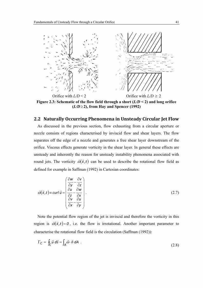
Fundamentals of Unsteady Flow through a Circular Orifice 41
Orifice with L/D < 2
Orifice with L/D ≥ 2
Figure 2.3: Schematic of the flow field through a short (L/D < 2) and long orifice (L/D ≥ 2), from Hay and Spencer (1992)
2.2 Naturally Occurring Phenomena in Unsteady Circular Jet Flow As discussed in the previous section, flow exhausting from a circular aperture or
nozzle consists of regions characterised by inviscid flow and shear layers. The flow
separates off the edge of a nozzle and generates a free shear layer downstream of the
orifice. Viscous effects generate vorticity in the shear layer. In general these effects are
unsteady and inherently the reason for unsteady instability phenomena associated with
round jets. The vorticity ( )t,x
R can be used to describe the rotational flow field as
defined for example in Saffman (1992) in Cartesian coordinates:
( )
∂∂
−∂∂
∂∂
−∂∂
∂∂
−∂∂
=≡
yu
xv
xw
zu
zv
yw
ucurlt,x
R .
( 2.7)
Note the potential flow region of the jet is inviscid and therefore the vorticity in this
region is ( ) 0t,x =
R , i.e. the flow is irrotational. Another important parameter to
characterise the rotational flow field is the circulation (Saffman (1992)):
∫∫ ⋅==ΓACC dAnsdu
R .
( 2.8)

Fundamentals of Unsteady Flow through a Circular Orifice 42
The circulation is defined as a line integral of the velocity u
around a curve C
surrounding a rotational flow element. Using Stoke’s theorem the vorticity can also be
expressed as the sum of the vorticity R through the area A enclosed by the curve C,
where n
is the normal vector on surface A.
The interaction of the vorticity within the free shear layer of the jet can cause the
development of coherent structures and ultimately lead to flow instabilities. Michalke
(1972) shows a flow visualisation of the vorticity structures in the free shear layer of a
round jet which agrees well with the schematic and description shown in Yule (1978)
(Figure 2.4). The schematic shows the growth of a flow instability in the shear layer of a
jet flow characterised by laminar and turbulent flow regimes. Initially, near the exit
nozzle of the jet, natural instabilities in the laminar shear layer produce regions of
vorticity in the form of small scale vortex ring structures. These structures travel
downstream in the shear layer of the jet and interaction with surrounding vortex ring
structures can cause the vortex rings to merge, thereby forming a large scale vortex ring
structure or a vortex puff as described in Crow and Champagne (1971). This
phenomenon is known as self-excited jet instability or the “preferred mode” of a jet
(Hussain and Zaman (1981)) where the large scale structures occur periodically on a
characteristic time-scale associated with the jet flow, which is defined by the Strouhal
number. The Strouhal number is defined as the frequency f of the occurrence of the
structures, the nozzle diameter D and the mean jet velocity Ud:
dj U
fDSt = . ( 2.9)
According to Crow and Champagne (1971) the self-excited roll up of vortical structures
within the shear layer occurs at jet Strouhal numbers of 30.=jSt . The ring structures
interact with the shear layer of the jet and entrain air from the stagnant fluid outside the
jet flow as well as from the potential core within the jet flow (Figure 2.4). The vortex
rings develop instability waves within the vorticity field of the shear layer and the
interaction of the generated vortices results in the break-up of the large scale structure
within the turbulent flow region. Within the turbulent field large scale eddies are still
present but these structures are not circumferentially coherent unlike vortex rings (Yule

Fundamentals of Unsteady Flow through a Circular Orifice 43
(1978)). The structures then decay to smaller scales until they fully dissipate in the
turbulent field.
Figure 2.4: Free shear layer instability in a transitional jet downstream of a jet
nozzle, from Yule (1978)
2.3 Forced Unsteady Phenomena in Circular Jet Flow Over the years many authors have investigated the instabilities associated with jets
flows and their sensitivity to acoustic forcing (Brown (1935), Crow and Champagne
(1971), Heavens (1980), etc). The forcing of the jet can be conducted with an acoustic
pressure amplitude altering the static pressure upstream or downstream of a jet nozzle
periodically. The result of the pressure amplitude forcing is an unsteady velocity
amplitude. For the low amplitude forcing the velocity amplitudes are much lower than
the mean jet velocity (i.e. 1<<Uu ). In contrast unsteady velocity amplitudes larger
than the mean velocity are indicative of a high amplitude forcing regime (i.e. 1≥Uu ).
However the size of the unsteady velocity amplitude is not only dependent on the static
pressure amplitude, it is also dependent on the time scale of the applied forcing.

Fundamentals of Unsteady Flow through a Circular Orifice 44
If the time scale of the pressure oscillation is large, forces associated with the inertia
of the jet flow (due to the acceleration of the mass of the jet) are negligible compared to
the forces of the unsteady static pressure variation. Hence this regime can be described
as the quasi-steady jet flow regime where the inertial forces associated with the jet are
negligible. In this regime large perturbation pressure amplitudes will lead to large
velocity oscillations and vice versa. Alternatively, if the time scale of the pressure
oscillations is small, forces associated with the inertia of the jet flow, are significant
compared to the forces of the unsteady static pressure variation. Thus in this regime
large pressure oscillations will lead to reduced velocity oscillations due to the influence
of the inertial forces.
2.3.1 Low Amplitude Forcing Brown (1935) investigated large scale structures within acoustically forced jet flows
using flow visualization. It was observed that the occurrence of large scale vortices was
more pronounced if the jet was forced at certain frequencies. Acoustic forcing of the jet
at those Strouhal numbers also leads to the largest perturbation of the jet centreline
velocity. Hussain and Zaman (1980) investigated the coherent structures by forcing the
jet on its “preferred mode” (Stj = 0.3) and measured the velocity oscillations in the jet
flow using a hot wire anemometer. The flow visualisation conducted by Heavens (1980)
also showed large scale coherent vortices. Heavens (1980) noticed that the structures
travel with a velocity of 0.5 Ud. More recently Schram and Riethmueller (2002) used
particle image velocimetry (PIV) to investigate the acoustically forced flow field of a
round jet. In this case the pairing and merging of subsequent vortices was of particular
interest and it was shown that the entrainment is locally enhanced due to the vortex
pairing in the excited flow field.
2.3.2 High Amplitude Forcing (Vortex Rings) Another unsteady phenomenon relevant to pulsatile jet flows is the roll up and
generation of axisymmetric vortex rings which pinch off the edge of the jet nozzle. This
phenomenon occurs if the jet flow is forced in such a way that reverse flow occurs
during one time period of excitation, e.g. synthetic jets (Jabbal et. al. (2006)) or non-
linear acoustic absorption (Ingard and Labate (1950)). Another possibility of generating

Fundamentals of Unsteady Flow through a Circular Orifice 45
a vortex ring is by an impulsive flow injection using a piston (Didden (1979)). The latter
is used to show a flow visualization from Didden (1979) in Figure 2.5 to discuss the
formation of a vortex ring.
Figure 2.5: Formation of a vortex ring from Didden (1979)
A piston was used to eject water through a nozzle into a water tank. Dye was injected
at the edge of the nozzle to visualize the formation of the vortex ring. The piston was
accelerated within the initial 0.3s. Afterwards the fluid was pushed through the nozzle at
a constant flow speed. At 1.6s the piston reached the end position and the jet velocity
dropped to zero. It can be seen that during the ejection period the shear layer rolls up at
the edge of the jet nozzle. Due to rotation of the vortex sheet, fluid from the potential
velocity field of the jet is entrained, and this increases the size of the ring vortex further.
Moreover the rotational flow field induces a velocity field which causes the vortex ring
to pinch off from the rim of the jet nozzle just before the end of the piston stroke. From
then on the vortex ring propels itself away from the nozzle edge while some of the
vorticity containing shear layer generates an opposite rotation on the inside of the
nozzle edge (1.66s onwards).
Figure 2.6 shows a simplified example of a vortex ring (e.g. (Maxworthy (1977))
where y represents the axial coordinate, x represents the radial coordinate, F the
azimuthal coordinate. As a first approximation the vortex ring is assumed to be

Fundamentals of Unsteady Flow through a Circular Orifice 46
axisymmetric, hence the flow field is constant along the azimuthal coordinate.
Moreover the vortex core itself is described by the cylindrical coordinate system (y’, Φ,
x’). The vorticity is concentrated within the core of the vortex ring. Thus the core of a
vortex ring is dominated by rotational flow. The core of an ideal vortex is also referred
to as a forced vortex (e.g. Douglas et. al. (2005)) which is characterised by a constant
angular velocity. A second region of the vortex flow field is the free vortex which
surrounds the forced vortex core. This region is irrotational and thus some text books
describe it as the potential vortex (Douglas et. al. (2005)). However in the case of vortex
rings which occur in engineering flow fields the differentiation is not as simple. Many
researchers have investigated methodologies to identify the size of the vortex core
radius RC (e.g. Jeong and Hussain (1995), Schram and Riethmueller (2001), Graftieaux
et. al. (2001), Kolar (2007), etc). Vortex rings are classified according to their
nondimensional size VRVC RR (e.g. Batchelor (2000)) where the parameter RVR denotes
the radius of the vortex ring. The radius of the vortex ring is defined as the distance of
the centre of the vortex core (y’-axis) to the centre of the vortex ring on the y-axis (see
Figure 2.6). Semi-empirical expressions for the kinetic energy and velocity of the vortex
rings are available for thin vortex rings ( 1<<VRVC RR ) as shown for example in
Sullivan et. al. (2008) or Saffman (1992):
Kinetic energy
−Γ= αρ
VC
VRVRCK R
RRE
821 2 ln ( 2.10)
Velocity of ring vortex
−
Γ= β
π VC
VR
VR
CV R
RR
U8
4ln , where 1−= αβ . ( 2.11)
The parameter β and the core radius RVC were chosen according to Saffman (1970):
558.0=β , TRVC ν4= where T was the duration of the piston stroke which generated
the vortex ring and ν represents the kinematic viscosity. Sullivan et. al. (2008) used
those expressions with reasonable agreement compared to their experimental data.
As indicated in the schematic of Figure 2.6 the vorticity distribution does not
necessarily drop to zero outside the vortex core. Maxworthy (1977) defined the core of
the vortex ring at the maximum velocity 22 vuu += using the maximum measured

Fundamentals of Unsteady Flow through a Circular Orifice 47
velocity along the core radius using Laser Doppler Velocimetry. In this case only 50%
of the total vorticity ( xvyu ∂∂−∂∂=φR ) was within the core of the vortex ring.
y,v
x,u
y’,v
x’,u
RVR
RVC
φR
x’
-RVC
u
Vorticity distribution Velocity distribution
Vortex core
x’
Figure 2.6: Schematic of vortex ring
Gharib et. al. (1998) measured the circulation of vortex rings using particle image
velocimetry during the formation of vortex rings. The vortex rings were formed using a
piston pushing fluid in a water tank similar to Didden (1979). A parameter quantifying
the energy put into the vortex ring is its formation number which was defined in Gharib
et. al. (1998) as
DtU
DL P=0 . ( 2.12)
The formation number relates the piston stroke length L0 to the orifice diameter D.
Moreover the stroke length can also be expressed by the mean piston velocity PU
multiplied by the time duration t for the piston stroke. Gharib et. al. (1998) found that
the circulation in the core of the vortex ring increases for formation numbers up to
40 ≈DL . Thereafter the total circulation of the vortex ring increased but the core
circulation remained constant. This leads to secondary flow features downstream of the
vortex rings such as wakes and secondary vortex rings which account for the general
increase in circulation. Similar observations were made by Jabbal et. al. (2006).
Hence the flow field of a vortex ring generated by an acoustic wave in the non-linear
absorption regime will be strongly dependent on the pressure amplitude. Thus the onset
of secondary flow fields or the transition from laminar to turbulent vortex rings, as

Fundamentals of Unsteady Flow through a Circular Orifice 48
described by Glezer (1988), could be important for the amount of non-linear acoustic
absorption attainable (i.e. where the unsteady flow field is generated by an acoustic
pressure oscillation rather than a moving piston).
2.4 Fundamentals of Acoustics This section will give a brief overview into the propagation of one dimensional plane
acoustic waves. In this work only linear acoustic oscillations are considered. This means
that the acoustic pressure amplitude 'p is much smaller than the ambient pressure p
within the fluid, i.e. p'p << . The fluctuating pressure and velocity can be described as
(Dowling and Stow (2003)):
( ) )t,x('ppt,xp += and ( ) )t,x('uut,xu += . ( 2.13)
The acoustic oscillation is treated as a harmonic oscillation so that the fluctuating
pressure and velocity are defined as:
( ) ( ) ( )tiexpxpt,x'p R= and ( ) ( ) ( )tiexpxut,x'u R= . ( 2.14)
The parameters p and v denote the time independent pressure and velocity
amplitudes. For an acoustic plane wave these quantities are only dependent on the axial
location. Furthermore the exponential function is the harmonic variation of the unsteady
pressure and velocity in time (t). The parameter R represents the angular frequency of
the oscillation.
2.4.1 The Acoustic Wave Equation The propagation of plane waves in an isothermal duct can be derived using a mass
conservation and an inviscid momentum balance for an ideal gas in a control volume as
introduced earlier in equations ( 2.1) and ( 2.2). Initially only acoustic oscillations in the
absence of mean flow are considered, i.e. 0=U . Substituting equations ( 2.13) into the
mass and momentum equations ( 2.1) and ( 2.2) and linearising the equations leads to the
unsteady form of the linear mass and momentum equations in the axial direction (e.g.
Schuermans (2003) or Dowling and Stow (2003)):

Fundamentals of Unsteady Flow through a Circular Orifice 49
0x'u
t'
=∂∂
+∂∂
ρρ
and ( 2.15)
0x'p
t'u
=∂∂
+∂∂
ρ . ( 2.16)
Differentiating equation ( 2.15) with respect to time and differentiating equation ( 2.16)
with respect to the axial coordinate x, and using the isentropic expression for pressure
and density '''' pcpp 21=⇔= ρρργ leads to the well-known acoustic wave
equation (e.g. Dowling and Stow (2003) or Schuermans (2003)):
0x
'pt
'pc1
2
2
2
2
2 =∂∂
−∂∂
. ( 2.17)
In the case where a uniform mean flow is present it can be shown that the wave
equation can take a similar form by using a coordinate transformation (as for example
shown in Schuermans (2003)). Therefore the convective acoustic wave equation can be
defined as (e.g. Schuermans (2003), Dowling and Stow (2003)):
0x
'pDt
'pDc1
x'p
'px
utc
12
2
2
2
22
22
2 =∂∂
−=∂∂
−
∂∂
+∂∂
. ( 2.18)
2.4.2 Plane Acoustic Waves For plane acoustic waves in a 1D duct the exact solution of the wave equation can be
defined as (e.g. Dowling and Stow (2003)):
( ) ( )cxtgcxtf)t,x('p ++−= ( 2.19)
and the acoustic velocity perturbation is described as
( ) ( )( )cxtgcxtfc
1)t,x('u +−−=
ρ. ( 2.20)
The parameters f and g are also known as Riemann invariants. In general equation
( 2.19) describes the acoustic pressure oscillation at every position x along a duct (Figure
2.7) as the superposition of two acoustic waves, one wave travelling in the positive axial
direction (f) and the other travelling in the negative axial direction (g).

Fundamentals of Unsteady Flow through a Circular Orifice 50
x
fg
Figure 2.7: Example of plane acoustic waves in a 1D duct
In this work the Fourier transformed versions for the expressions of acoustic pressure
and velocity are used:
( ) ( ) ( )xiktipxiktiptixp −−++ ++−= RRR expˆexpˆexp)(ˆ and. ( 2.21)
( ) ( ) ( )( )xiktipxiktipc
tixu −−++ +−−= RRρ
R expˆexpˆexp)(ˆ 1 ( 2.22)
The circumflex denotes that the parameters are complex amplitudes and the variables
k+ and k- represent the wave numbers for acoustic waves travelling with (+) and against
(-) the mean flow direction. Thus the wave numbers are defined as
( )M1ck
±=±
R. ( 2.23)
In this case M denotes the mean flow Mach number within the duct. If the complex
amplitudes of the downstream and upstream travelling waves are known the acoustic
pressure and the velocity oscillation at any axial position x can be determined.
A useful acoustic parameter to describe various acoustic elements or boundary
conditions is the specific acoustic impedance which relates the acoustic pressure
amplitude to the acoustic velocity oscillation (Kinsler et. al. (2000) or Beranek (1954))):
up
Z = . ( 2.24)
A more convenient way to describe the impedance is to use the acoustic volume
velocity using the cross-sectional area of a duct A (Kinsler et. al. (2000)):
AupZˆˆ
= . ( 2.25)

Fundamentals of Unsteady Flow through a Circular Orifice 51
2.4.3 Acoustic Energy Flux The acoustic intensity for plane waves in a duct with mean flow can be defined as (e.g. Morfey (1971)):
222 11pM
cupMpM
cupI ′++′+=
ρρ'''' . ( 2.26)
Integrating the intensity across the duct area leads to the flux of acoustic energy as
defined in (Blokhintsev (1946), Heuwinkel et. al. (2007)):
( )22
12
MAc
p+=Π +
+ ρ
ˆ and ( 2.27)
( )22
12
MAc
p−=Π −
− ρ
ˆ. ( 2.28)
The parameter A represents the cross-sectional area of the tube and M denotes the mean
Mach number of the flow in the tube. Note in this work the Mach number was much
smaller than one. Hence the Mach number terms in (2.26) to (2.28) have negligible
influence.
2.4.4 Acoustic Absorption Coefficient The acoustic absorption of a test specimen exposed to plane acoustic waves upstream
and downstream of the test section (Figure 2.8) can be characterised by the acoustic
absorption coefficient.
+up
−up −p
Mean flow direction
+usp
−usp −
ds
Mean flow direction
+pds
Figure 2.8: Example of plane waves upstream and downstream of a test specimen In this case the test specimen consists of a circular orifice disc through which a mean
flow passes. Hence the absorption coefficient can be calculated using the stagnation
enthalpy as defined in Eldredge and Dowling (2003):
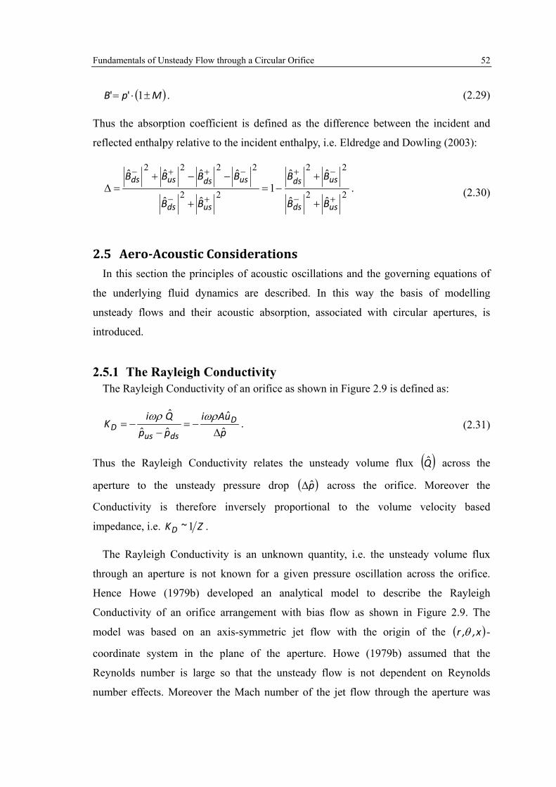
Fundamentals of Unsteady Flow through a Circular Orifice 52
( )MpB ±⋅= 1'' . ( 2.29)
Thus the absorption coefficient is defined as the difference between the incident and
reflected enthalpy relative to the incident enthalpy, i.e. Eldredge and Dowling (2003):
22
22
22
2222
1+−
−+
+−
−++−
+
+−=
+
−−+=∆
usds
usds
usds
usdsusds
BB
BB
BB
BBBB
ˆˆ
ˆˆ
ˆˆ
ˆˆˆˆ.
( 2.30)
2.5 Aero-Acoustic Considerations In this section the principles of acoustic oscillations and the governing equations of
the underlying fluid dynamics are described. In this way the basis of modelling
unsteady flows and their acoustic absorption, associated with circular apertures, is
introduced.
2.5.1 The Rayleigh Conductivity The Rayleigh Conductivity of an orifice as shown in Figure 2.9 is defined as:
puAi
ppQi
K D
dsusD ˆ
ˆˆˆ
ˆ
∆−=
−−=
RρRρ. ( 2.31)
Thus the Rayleigh Conductivity relates the unsteady volume flux ( )Q across the
aperture to the unsteady pressure drop ( )p∆ across the orifice. Moreover the
Conductivity is therefore inversely proportional to the volume velocity based
impedance, i.e. ZKD 1~ .
The Rayleigh Conductivity is an unknown quantity, i.e. the unsteady volume flux
through an aperture is not known for a given pressure oscillation across the orifice.
Hence Howe (1979b) developed an analytical model to describe the Rayleigh
Conductivity of an orifice arrangement with bias flow as shown in Figure 2.9. The
model was based on an axis-symmetric jet flow with the origin of the ( )x,,r θ -
coordinate system in the plane of the aperture. Howe (1979b) assumed that the
Reynolds number is large so that the unsteady flow is not dependent on Reynolds
number effects. Moreover the Mach number of the jet flow through the aperture was

Fundamentals of Unsteady Flow through a Circular Orifice 53
assumed to be low to enable the flow to be treated as incompressible. A harmonic
pressure oscillation usp′ upstream of the orifice drives an unsteady flow through the
orifice. Howe (1979b) assumed that the orifice is infinitesimally thin and the jet flow
through the orifice is irrotational. To avoid singularities at the edge of the aperture, due
to the inviscid jet flow, it is assumed that vorticity is shed at the edge of the aperture rim
as this is known from the Kutta-condition (from inviscid flow over aerofoils). The
vorticity is a succession of vortices with infinitesimally small cores which generate a
cylindrical sheet downstream of the orifice at x > 0 and r = R.
Vorticity layer
( )tipp usus Rexpˆ=′
D
r
x
O
( )tipp dsds Rexpˆ=′
Figure 2.9 Schematic of unsteady orifice flow field, as in Howe (1979b) The pressure and velocity perturbation is described with the use of the stagnation
enthalpy B:
( )tiBvpB Rρ
expˆ=+= 221 . ( 2.32)
Howe (1979b) then used the divergence of the momentum equation of the unsteady
jet flow with a thin vorticity sheet at the edge of the aperture as:
( )vdivB2 ×−=∇ R . ( 2.33)
In this case the vorticity vector is defined as 'RRR
+= . Howe (1979b) has investigated
the right hand side of this equation in more detail and defined the linearised version of
the cross product as:
UUvv ×+×+×=× RRRR
'' . ( 2.34)
A further assumption was that the radial length scale of the shed vorticity is much
smaller than the shear layer thickness. Hence the radial component of 'v can be

Fundamentals of Unsteady Flow through a Circular Orifice 54
neglected and therefore only the second term within equation ( 2.34) is important to
calculate the effect of the shed vorticity. This was previously utilized to predict the
behaviour of a jet flow exiting from a nozzle (Howe (1979a)). Thus equation ( 2.33)
reduces to:
( )U'divB2 ×−=∇ R . ( 2.35)
Moreover it was assumed that the vortex rings generated by the vorticity oscillation 'R
are travelling with constant axial velocity U . Hence on the basis of the described
assumptions the vorticity fluctuation due to the incident pressure oscillation can be
defined as:
( ) ( ) ( )UxitiRrxHe RRδσR θR −−−= exp' . ( 2.36)
The Heaviside function H(x) ensures that vorticity is only shed downstream of the
orifice ( 0x ≥ ). Moreover the Dirac delta function satisfies the assumption that vorticity
is only shed within an infinitesimal thin cylindrical shear layer of radius R. The
parameter σ represents the amplitude of the shed vorticity per unit length.
Differentiating the vorticity and substituting it into equation ( 2.35) whilst assuming an
axisymmetric flow field leads to:
( ) ( )
−
−=
∂
∂+
∂∂
∂∂ x
UiRrxH
rUR
x
BrBr
rrRδ
σ R exp'2
21 . ( 2.37)
The equation was solved analytically as shown in Howe (1979b) by deriving a solution
for the circulation amplitude of the shed vorticity. Howe (1979b) then used the solution
of the inhomogeneous Poisson equation to derive an expression for the Rayleigh
Conductivity:
( ) ( )( )StiStRppuAi
Kdsus
DR δ
Rρ−Γ=
−−= 2
ˆˆˆ
. ( 2.38)
The parameters Γ and δ (Figure 1.8) are solely dependent on the Strouhal number. In
this case I1 and K1 are modified Bessel functions and the definition of the inertia and the
admittance follows from the solution of equation ( 2.37):

Fundamentals of Unsteady Flow through a Circular Orifice 55
( ) ( ) ( ) ( ) ( )( )
( ) ( ) ( ) ( )21
22
21
212
21
StKStcoshSt2exp4
StI
StStsinh
StcoshStKStcoshSt2exp4
St1
1StI
π
πΓ
+
−+
+
= ,
( 2.39)
( ) ( ) ( )
( ) ( ) ( ) ( )21
22
21
11
StKStcoshSt2exp4
StI
St2expStKStISt
2
π
πδ
+= .
( 2.40)
Furthermore the Strouhal number was defined based on the orifice radius R and the
angular frequency R as
UR
URf
StRπ
==2
. ( 2.41)
According to Howe (1979b), the mean velocity parameter U represents the vortex
sheet velocity, which was estimated to dUU 50.= . Moreover the asymptotic analysis in
Howe (1979b) suggests that the contraction ratio between the area of the vena contracta
and the area of the aperture was also calculated to be 0.5. Thus for the purpose of this
work the mean bias flow velocity in the plane of the aperture DU will be used as an
assumption for the mean vortex sheet velocity. Hence the Strouhal number definition in
equation (1.16).
The acoustic energy dissipated due to the unsteady pressure oscillation across the
orifice can be defined as in Luong et. al. (2005):
( )( ) ( )( )dttiexppRetiexpQReT1 T
0L ∫= R∆RΠ .
( 2.42)
This represents the flux of acoustic energy through the orifice assuming
incompressible orifice flow (i.e. M <<1). Using the Rayleigh Conductivity model form
Howe (1979b) an averaged loss of acoustic energy (Luong et. al. (2005)) can be
defined, which is dependent on the admittance (δ), the unsteady pressure amplitude
( p∆ ), the radius of the orifice (R), the density (r) and the frequency (ω):

Fundamentals of Unsteady Flow through a Circular Orifice 56
ρRδ
∆ΠR
p 2L = . ( 2.43)
Over the years various modifications to the Rayleigh Conductivity model defined by
Howe (1979b) have been undertaken. Wendoloski (1998) solved the divergence of the
momentum equation as defined in ( 2.37) taking the effects of the open area ratio, or
porosity, between the upstream channel and the orifice into account.
Moreover a numerical solution was used by Jing and Sun (2000) to extend the shed
vorticity amplitudes, as defined by Howe (1979b), to an orifice plate with finite
thickness. Therefore the expression of the unsteady vorticity as defined in ( 2.36) was
modified to:
( ) ( )Usitine s RRδσR θR −−= exp' . ( 2.44)
In this case the shear layer was defined using a jet profile as in Rouse and Abul-
Fetouh (1950) instead of the assumption of a cylindrical shear layer. Hence the shed
vorticity oscillation is dependent on the vortex stream line s and the coordinate normal
to the vortex stream line ns. However the data in Rouse and Abul-Fetouh (1950) was
measured for infinitesimal thin orifice plates at various contraction ratios between the
orifice and a feed tube. Thus, strictly speaking, the profiles are only valid for
infinitesimal thin L/D ratios. Therefore the assumption in this case is that the jet profiles
do not change for the range of investigated L/D ratios in Jing and Sun (2000). The
divergence of the resulting inhomogeneous Poisson equation could not be solved
analytically. Hence a boundary element method was used to solve the equation
numerically. The Conductivity derived by Jing and Sun (2000) is shown in Figure 2.10.
This figure is taken from Jing and Sun (2000) and the parameters have been adopted to
suit the nomenclature of this work. It was not part of this work to compute the equations
derived by Jing and Sun (2000). It can be seen that the conductivity varies with aperture
length-to-diameter ratio L/D. The solution with length-to-diameter ratio of 0.0 is
identical to the Conductivity model from Howe (1979b). The model was used and
compared to some experimental data from impedance measurements for perforated
liners. It can be seen in Jing and Sun (2000) that the model agreed with the trends in the
experimental data. It was also mentioned that the developed model was not valid if

Fundamentals of Unsteady Flow through a Circular Orifice 57
reattachment of the flow field within the orifice occurs, i.e. L/D ~ 2. A description of
this model can also be found in Lee et. al. (2007) who extended the theory to include
orifice interaction effects between apertures in perforated liners.
Figure 2.10: Rayleigh Conductivity from Jing and Sun (2000)
2.5.2 Modifications to the Rayleigh Conductivity Model Of more significance to this work is the work of Jing and Sun (1999), who introduced
a length correction to the Rayleigh conductivity as defined by Howe (1979b). In this
way more practical engineering applications could be investigated. In this case the
normalised acoustic impedance for an orifice was used:

Fundamentals of Unsteady Flow through a Circular Orifice 58
ucpz
ˆˆ
ρ= . ( 2.45)
Using the Rayleigh Conductivity model from Howe (1979b) and substituting for the
unsteady velocity in the normalized acoustic impedance leads to the expression for the
normalized acoustic impedance of an orifice as described in Jing and Sun (1999):
Γ+
Γ−
Γ+=
−= 22222 δδ
δπR icR
upp
zD
usdsˆ
ˆˆ. ( 2.46)
Note that the wave number k is defined as ck R= . Jing and Sun (1999) compared the
derived normalized specific impedance of the orifice with the impedance for a tube
without mean flow. The impedance of the tube was taken from Beranek (1954) for the
condition f01.0R > (which is also valid for every orifice investigated in this work):
cL
iRL
czT
RνR−=
2 . ( 2.47)
In this case the resistance of the orifice is caused by the viscosity of the boundary layer
within the tube. Hence the use of the kinematic viscosity ν. The frequency is expressed
using the parameter ω and the thickness or length of the tube is described by the
parameter L. The reactance of the impedance ( )cLR is due to the mass of the fluid
within the tube. Note the length of the orifice within the reactance term can also include
an acoustic length correction. Jing and Sun (1999) neglected the resistance part of the
impedance as the length-to-diameter ratio was small and therefore the viscous effects
negligible. Using this methodology the normalised impedance for the orifice, based on
the Rayleigh Conductivity by Howe (1979b), was extended with the inertia part due to
the increased mass within an orifice of physical length (Jing and Sun (1999)):
Lc
iicRztot
R
δδ
δπR−
Γ+
Γ−
Γ+= 22222
. ( 2.48)
Jing and Sun (1999) compared this expression to their measurements of perforated
liners within an impedance tube for apertures with length-to-diameter ratios up to L/D =
0.65. The experiments showed good agreement with the measured data. Moreover many

Fundamentals of Unsteady Flow through a Circular Orifice 59
other authors used the modified Rayleigh Conductivity model with acoustic absorption
models for perforated liners, e.g. Eldredge and Dowling (2003).
2.5.3 Non-Linear Absorption Modelling Over the years many authors have associated the non-linear acoustic damping
mechanism of an unsteady orifice flow field with large scale vortex ring structures
(Ingard and Labate (1950), Zinn (1970), Whiffen and Ahuja (1983),Tam et. al. (2001),
Jing and Sun (2002), Lebedeva et. al. (2005), etc.). To illustrate this Figure 2.11 shows
an orifice which is surrounded by an harmonic acoustic pressure field upstream ( usp′ )
and downstream ( dsp′ ) of the orifice. In this case there is no mean flow entering and
exiting the aperture. The acoustic pressure oscillation causes an unsteady velocity
perturbation 'u in the orifice. Subsequently the pulsatile velocity generates a vortex
sheet at the edge of the orifice. In the absence of a mean flow field the velocity
oscillation changes direction during one time period of an acoustic cycle. In other words
the flow is reversing during one half of the acoustic cycle.
Vortex ring( )tipp dsds Rexpˆ=′( )tipp usus Rexpˆ=′
Induced mean velocity fieldD
Aco
ustic
term
inat
ion
At
Figure 2.11: Schematic of large scale structures associated with non-linear absorp-
tion As a consequence of the fluid motion large scale flow structures are generated as the
vorticity sheet rolls up into a vortex ring at the edge of the aperture. Subsequently the
vortex rings pinch off at the rim of the aperture. Due to the rotation of the vortex a
velocity field is induced in the centre of the vortex ring which propels the vortex ring
away from the orifice. In this way acoustic energy is transferred into the kinetic energy
of the large scale vortex ring structures which subsequently dissipate into turbulence
and heat further away from the orifice exit. Note that with no mean flow present vortex
rings occur on either side of the orifice. Over the years many authors developed

Fundamentals of Unsteady Flow through a Circular Orifice 60
modelling techniques for the non-linear relationship between the pressure oscillation
and the velocity oscillation, e.g. Ingard (1970), Zinn (1970), Cummings and Eversman
(1983), Cummings (1986), Keller and Zauner (1995), Bellucci et. al. (2004), etc. A
summary of the developed methods is given here to highlight some of the assumptions
and challenges for the developed models. Moreover added mean flow across the
aperture can cause the absorption mechanism to transition between the linear and non-
linear absorption regime dependent on the ratio of unsteady velocity amplitude to mean
velocity. This complexity is also included within the modelling techniques introduced in
this section.
A momentum balance, as shown in the steady case for incompressible flow (Ingard
(1970), Cummings (1986), Bellucci et. al. (2004)) can be used to describe the non-linear
acoustic behaviour of an orifice within a duct:
DeffDvisLDDusds UlUUUpp ρρζζρ −−−=−21 .
( 2.49)
Note that in this case the velocity UD in the plane of the aperture is used. Hence the
occurrence of a loss coefficient ζL compared to, for example, the Bernoulli equation
( 2.3) in section (2.1) which was defined using the velocity at the end of the vena
contracta. According to Ingard (1970) the loss coefficient can be described based on the
discharge coefficient:
2D
L C1
=ζ , ( 2.50)
whereas Cummings (1986) also includes the porosity of the orifice (ratio between open
area and total area of the orifice plate):
2D
2D
2
L CC1 σ
ζ−
= . ( 2.51)
Alternatively Bellucci et. al. (2004) uses a high Reynolds number loss coefficient
dependent on flow direction and area contraction upstream and downstream of the
orifice as defined in Batchelor (2007). The second term on the right hand side takes
viscous losses (ζvis), due to the boundary layer within the orifice, into account (Bellucci

Fundamentals of Unsteady Flow through a Circular Orifice 61
et. al. (2004)). Inertia effects due to the mass of the fluid within the orifice are
accounted for by the last term on the right hand side, which includes the physical length
and the length corrected parts of the orifice (Ingard (1970), Cummings (1986) and
Bellucci et. al. (2004). Substituting the mean and harmonic velocity and pressure
oscillations according to equations ( 2.13) and ( 2.14) into the momentum equation ( 2.49)
leads to:
DeffDvisusds UlUpp ′−′−Φ−=′−′ ρρζ . ( 2.52)
Note the viscous component due to the mean flow is negligible. The non-linear pressure
loss term Φ in the momentum equation ( 2.52) is then defined as (Bellucci et. al. (2004)):
( )( )DDDDDDL UUUUUU −′+′+=Φ ρζ21 . ( 2.53)
Keller and Zauner (1995) derived a solution for the pressure loss term, including the
presence of mean flow through the aperture, using a Fourier expansion of the non-linear
velocity term DD uu ′′ . Only using the fundamental harmonics of the Fourier expansion
lead to the pressure loss term defined by Bellucci et. al. (2004) in the frequency domain:
DDD
DL uu
uU
g ˆˆˆ
ˆ
=Φ ρς . ( 2.54)
The assumption of using the fundamental harmonics of the Fourier expansion is valid
based on the experiments and analytical investigations in Ingard (1970) showing a
significant reduction in velocity amplitudes for harmonics larger than the fundamental
frequency.
The function ( )DD uUg ˆ is defined as in Keller and Zauner (1995) or Bellucci et. al.
(2004):
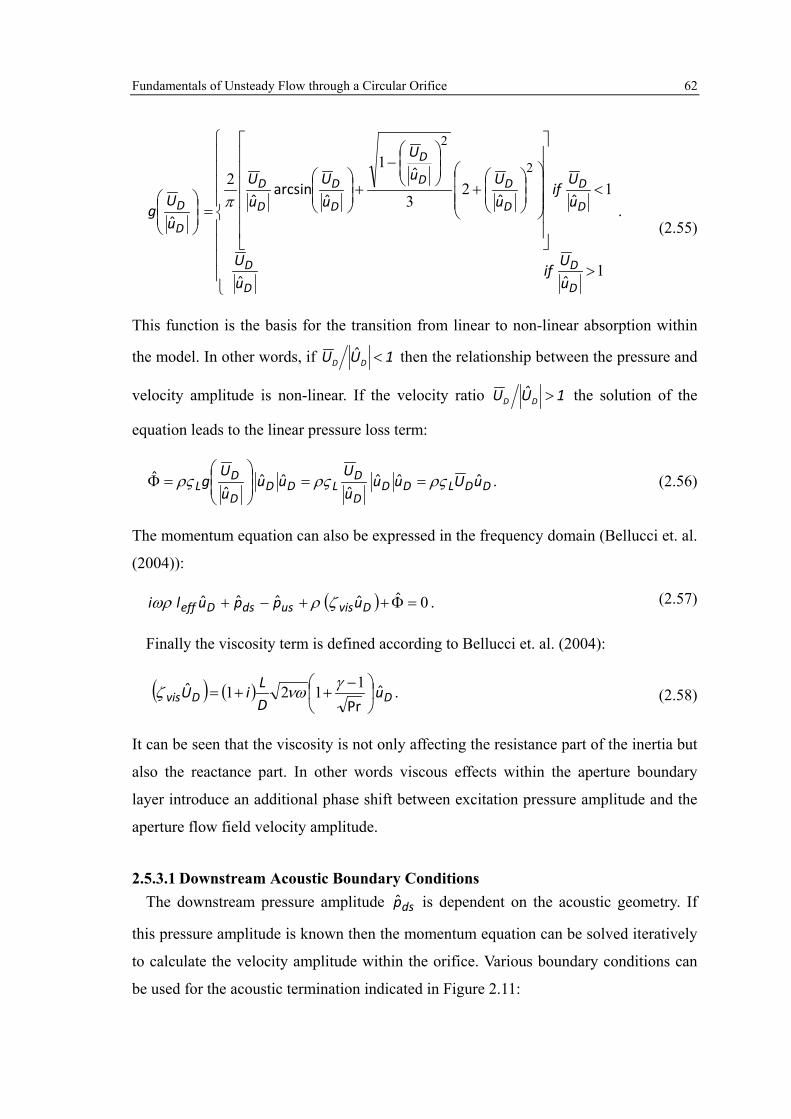
Fundamentals of Unsteady Flow through a Circular Orifice 62
>
<
+
−
+
=
1
123
12
2
2
D
D
D
D
D
D
D
DD
D
D
D
D
D
D
D
uU
ifuU
uU
ifuUu
U
uU
uU
uU
g
ˆˆ
ˆˆ
ˆ
ˆarcsin
ˆˆ
π .
( 2.55)
This function is the basis for the transition from linear to non-linear absorption within
the model. In other words, if 1UU DD < then the relationship between the pressure and
velocity amplitude is non-linear. If the velocity ratio 1UU DD > the solution of the
equation leads to the linear pressure loss term:
DDLDDD
DLDD
D
DL uUuu
uU
uuuU
g ˆˆˆˆ
ˆˆˆ
ˆ ρςρςρς ==
=Φ . ( 2.56)
The momentum equation can also be expressed in the frequency domain (Bellucci et. al.
(2004)):
( ) 0=Φ++−+ ˆˆˆˆˆ DvisusdsDeff uppuli ζρRρ . ( 2.57)
Finally the viscosity term is defined according to Bellucci et. al. (2004):
( ) ( ) DDvis uDLiU ˆ
Prˆ
−++=
1121 γνRζ . ( 2.58)
It can be seen that the viscosity is not only affecting the resistance part of the inertia but
also the reactance part. In other words viscous effects within the aperture boundary
layer introduce an additional phase shift between excitation pressure amplitude and the
aperture flow field velocity amplitude.
2.5.3.1 Downstream Acoustic Boundary Conditions The downstream pressure amplitude dsp is dependent on the acoustic geometry. If
this pressure amplitude is known then the momentum equation can be solved iteratively
to calculate the velocity amplitude within the orifice. Various boundary conditions can
be used for the acoustic termination indicated in Figure 2.11:

Fundamentals of Unsteady Flow through a Circular Orifice 63
i) Anechoic boundary condition
In the case of an anechoic termination the downstream pressure amplitude can be
defined using the characteristic impedance (rc) as in Ingard (1970):
Dt
ds ucAD
p ˆˆ ρπ
=
4
2. ( 2.59)
ii) Plenum boundary condition
If the downstream termination consists of a plenum then the downstream pressure
amplitude would be equal to zero: 0=dsp .
iii) Helmholtz resonator
For the orifice being attached to a resonating volume, as for example in a Helmholtz
resonator, the pressure amplitude in the cavity can be calculated by using a mass
balance within the resonator volume (e.g. Bellucci et. al. (2004)):
DD AUt
Vt
m′−=
∂′∂
=∂
′∂ρ
ρ. ( 2.60)
Assuming an isentropic compression and expansion due to the oscillating mass flow and
transferring the equation into the frequency domain leads to the expression for the
pressure amplitude within the resonator volume:
DDds AuV
cip ˆˆ
Rρ 2
= . ( 2.61)
2.5.3.2 Acoustic Energy Loss Calculation The expressions for the downstream pressure amplitudes together with the momentum
equation can be used to solve for the velocity perturbation within the orifice. Loss of
acoustic energy is associated with the flux of the energy within the orifice itself
(Bellucci et. al. (2004)):
( ) OusDL Apu ˆˆRe *21
=Π . ( 2.62)

Fundamentals of Unsteady Flow through a Circular Orifice 64
The fluid dynamic loss mechanism Lζ as well as the length correction leff are not
necessarily known a priori and are often derived empirically. However, these parameters
have a significant effect on the unsteady velocity amplitudes and hence upon the loss of
acoustic energy. Keller and Zauner (1995) showed in their investigations that the loss
coefficients changed by a large amount if there was a mean flow through the resonator.
Moreover their experiments showed that an improvement of the loss coefficient due to
rounded edges of the investigated resonator neck lead to an increase in measured
absorption. Hence the behaviour of fluid dynamic processes such as vortex rings will
have a large effect upon the parameters used to predict the non-linear absorption
characteristic correctly.

Experimental Facilities and Methods 65
3 Experimental Facilities and Methods In general the objective was to undertake a series of measurements to further
understand the fundamental absorption characteristic of isolated orifice plates
representative of apertures typically found in gas turbine combustors. Therefore an
isothermal acoustic test facility has been used at ambient pressure and temperature. The
test facility was adapted in various ways to allow the study of fundamental acoustic
absorption characteristics as well as more gas turbine combustion system representative
geometry in a cost effective manner. Thus simple acoustic test configurations were used
to study the fundamental acoustic absorption characteristics while measuring the
unsteady flow field surrounding the apertures. Thereafter more complex acoustic test
configurations have been used to investigate the damping characteristic of perforated
liners which are directly applicable to gas turbine combustors. In this case the findings
and modelling techniques developed during the fundamental single aperture
measurements were then applied to explore the optimisation of passive dampers suitable
for gas turbine combustion systems. The objectives of the various experimental facilities
used are summarised in Table 3.1. Each experiment was conducted under isothermal
atmospheric conditions at ambient pressure and temperature in the test facility shown in
Figure 3.1. The facility is arranged on three floors: the upper floor is used as a plenum,
the middle floor contains the test cell (where the test section is located) and the fan
room and the lower floor is used as another plenum. Each plenum has a volume of
approximately 50 m3 and acts as an open acoustic boundary condition for the acoustic
test sections. The air flow rate and flow direction through the rest rig can be controlled
with a centrifugal fan and suitable ducting. Either the air is drawn out of the lower
plenum or air is blown into the lower plenum. The air flow direction in Figure 3.1 is
indicated with blue arrows. A 120 mm diameter circular duct connects the lower plenum
with the test cell where the duct terminates with a flange arrangement. The flange is
used as an interface to the various test sections investigated during this work. Square
test sections have been connected to the test facility via the discussed flanged interface.
Hence an interface duct was manufactured for each test section with a smooth transition
piece from the round inlet duct to the rectangular test section to minimise acoustic

Experimental Facilities and Methods 66
losses and excessive acoustic reflections which would reduce the amount of acoustic
energy transferred into the test section.
Test Sections Objectives
Fundamental acoustic absorption and Rayleigh Conductivity meas-urements
• Acoustic absorption coefficient measure-ment
• Acoustic energy loss measurement
• Unsteady flow field measurement to inves-tigate interactions between the unsteady flow field and the linear and non-linear acoustic absorption characteristic.
• Develop validation data to assess the per-formance of analytical acoustic absorption models for gas turbine combustion system relevant aperture geometries over wide range of Strouhal numbers.
Multi-aperture perforated liner test section
• Measure the acoustic absorption of perfo-rated liners suitable to gas turbine com-bustion system design envelope.
• Validate analytical absorption models for multi aperture and multi skin acoustic dampers.
Single sector combustion system test section
• Measure the acoustic absorption character-istic under the influence of a complex fuel injector flow field.
• Validate analytical absorption models.
• Investigate gas turbine combustion system design envelope.
Table 3.1: Overview of test sections used for the investigation of fundamental ab-sorption characteristics
To generate plane acoustic waves two JBL AL6115 600 W loudspeakers were used
attached to the inlet duct in the lower plenum. The loudspeakers are driven by a Chevin
Research A3000 amplifier system. A reference to the acoustic driver system and the test
facility can be found in Barker et. al. (2005). The excitation frequency from the
loudspeakers for the conducted experiments ranges from 10 Hz to 1000 Hz and the
pressure amplitudes can vary between 115 dB- 145 dB for the test sections investigated
in this work.

Experimental Facilities and Methods 67
Interface to test section
Upper plenum ~ 50m3
Lower plenum ~ 50m3
Loud speaker
Test Cell Fan room
Centrifugal fan
Air flow
Louvers
Air flow
Figure 3.1: Schematic of the aero-acoustic test facility, not to scale
3.1 Scaling from Gas Turbine Engines to Experimental Test Rig Geometry
Before the developed test sections are discussed the relevant scaling from engine
applications to small scale isothermal experiments will be discussed. Scaling is
important so that the data measured in the ambient labscale environment is transferrable
between engine and test rig. Modern gas turbine aero-engine combustion systems
typically operate at approximately 40 bar combustor inlet pressure and 900 K inlet
temperature (take-off conditions). Note that the combustion temperatures downstream
of the liner are higher than 900 K, however for the performance of the perforated liner
the cooling air temperature passing through the apertures is the relevant quantity. In
comparison, the isothermal test facility operates at 1 bar and 290 K temperature. Hence
the relevant non-dimensional scaling parameters used in this investigation have to be

Experimental Facilities and Methods 68
identified to relate the atmospheric test results back to the full scale engine operating
conditions.
As already discussed the acoustic absorption due to perforated liners is mainly
dependent on the Strouhal number as defined by Howe (1979b). Hence:
RigD
Engine StU
RSt ==R ( 3.1)
Another important parameter for the scaling of passive damper geometry is the ratio
of incident pressure amplitude to mean pressure difference across the perforated liner,
i.e.:
nRig
pknEngine P
pp
P ==∆
. (3.2)
The pressure amplitude in this case was chosen as the 0-peak amplitude. As will be
subsequently shown this parameter has a direct influence on determining if the liner is
within the linear or non-linear regime.
Furthermore the Mach number which relates the velocity through the apertures to the
speed of sound was kept constant between the test rig and the engine:
Rigd
Engine Mc
UM == . (3.3)
The Mach number is linked to the mean pressure drop across the apertures. Moreover
the pressure drop across a gas turbine wall remains constant across the operating
envelope of the engine. Therefore the pressure drop (dp/p) within the atmospheric test
rig has to be the same to operate at the same Mach number through the apertures. The
pressure drop is defined as the mean pressure drop across the aperture related to the
upstream pressure:
Rigus
dsus
Engine pp
ppp
pp
∆=
−=
∆ . (3.4)
For convenience in this work the mean pressure drop across the apertures will be
referred to as dp/p.

Experimental Facilities and Methods 69
The impact of the Reynolds number on the scaling of the acoustic absorption test
configuration is of second order. This is valid as long as the Reynolds number is
sufficiently high above any transitional flow effects. Hence although the Reynolds
number could not be conserved for the measurements conducted in this work, it was
ensured that the Reynolds number was above any transitional effects.
As already discussed the aim was to assess combustion system relevant aperture
geometry. Therefore cooling ring, effusion tiles, primary port and single skin effusion
geometries need to be assessed. Table 3.2 shows an overview of the relevant geometries
on conventional and modern gas turbine combustors. The Strouhal numbers have been
estimated using combustor inlet pressures of 40 bar and 900 K inlet temperature. The
frequency depends on the size of the full annular combustion systems and hence a range
from 400 to 900 Hz was considered.
Orifice Type D in mm L/D Strouhal number St
Reynolds num-ber Re
Mean pres-sure drop
dp/p
Cooling ring 0.7…1 6…8 0.01…0.03 34000…50000 3%
Single effu-sion skin
0.7…1 >10 0.01…0.03 34000…50000 3%
Effusion tile 0.7…1 2…7 0.02…0.18 6000…29000 0.1 – 1%
Ports 10…20 ~0.5 0.14…0.65 490000…990000 3% Table 3.2: Combustor orifice geometries relevant to gas turbine engines
Combustor background noise levels have been estimated to be of order 150 dB at 40
bar pressure. Therefore the pressure amplitude scaling of equation (3.2) leads to 118 dB
pressure amplitude at ambient pressure for the relevant pressure drop across the
aperture. The pressure amplitude in dB is defined as:
⋅
⋅= −5rms
102p
10log20dB . (3.5)
Note that the amplitude used for the decibel scale is the root mean square amplitude
which can be calculated using the peak amplitude:
2
pp pk
rms = . (3.6)

Experimental Facilities and Methods 70
However pressure amplitudes due to a thermo-acoustic instability at 40 bar can rise to
190 dB, which is in the order of the combustor pressure drop at 40 bar combustor inlet
pressure. For the investigated orifice geometries the mean pressure drop ranges from 0
to 3%. Hence the scaled max amplitude for the isothermal condition ranges from 131 to
160 dB at ambient pressure. The maximum available pressure amplitude within the test
facility on the square duct dimensions is 145 dB. Hence the pressure amplitude
excitation range was set between 115 and 145 dB, and it is acknowledged that the very
high limit cycle amplitudes cannot be simulated.
For the experiments conducted the test sections were designed to ensure constant
Strouhal and Mach numbers between the test rig and the engine geometry. Moreover to
remain within the relevant absorption regime (i.e. linear or non-linear) the pressure
amplitudes were scaled relative to the aperture pressure drop to ensure similarity with
the engine pressure amplitude forcing. Therefore the diameter, excitation frequency and
excitation amplitudes were scaled according to the introduced non-dimensional
parameters.
3.2 Fundamental Investigation of the Acoustic Absorption by Circular Apertures
This section will describe the test facilities which have been used to conduct the
fundamental acoustic absorption investigations. Initially a single aperture test rig has
been used to measure the acoustic absorption whilst particle image velocimetry (PIV)
has been conducted. Thereafter the facility has been modified to increase the Strouhal
number range over which the Rayleigh Conductivity of the apertures could be
measured.
3.2.1 Acoustic Absorption Measurements and PIV Investigations The objective for the experiments in this section was to provide sufficient optical
access and accurate acoustic measurements to develop a methodology for the flow field
characterisation relevant to linear and non-linear acoustic absorption of circular orifice
plates. Therefore the unsteady flow field was measured during acoustic excitation using
a high speed particle image velocimetry (PIV) system. To avoid refraction in the optical
measurement technique a rectangular duct with a 120 mm by 120 mm cross-section was

Experimental Facilities and Methods 71
chosen. Moreover the test rig walls were made out of Perspex, again to allow optical
access, with a wall thickness of 20 mm to avoid structural vibration effects due to the
acoustic forcing. Furthermore the duct was also supported at regular intervals to keep
the structural resonance frequencies well above the acoustic excitation frequencies. The
area of the duct was sufficient to generate pressure amplitudes up to 145 dB which was
necessary for the non-linear absorption measurements at elevated mean pressure drops
across the orifice.
The experiments have been conducted at ambient conditions and a schematic of the
test section is shown in Figure 3.2. Descriptions of the same test facility can also be
found in Rupp et. al. (2010) and Rupp et. al. (2010b). Note that the blue arrows
represent air flow and the red arrows plane acoustic waves. The test rig inlet was in the
upper plenum and the mean flow exit was located in the lower plenum. Thus the
acoustic boundary conditions for the test rig were open boundary conditions (i.e. with
pressure amplitude equal to zero). In this case air was drawn from the upper plenum
through the test section and exhausted via the lower plenum. The test section consists of
a flange to which suitable orifice plates could be attached. These plates were of varying
thickness (L) and contained orifices of varying diameter (D). It is worth noting that in
these experiments the orifice behaviour is investigated without interaction effects from
neighbouring apertures. Thus the test specimens represent a single aperture within a
perforated liner where the aperture pitch (P) is large enough to ensure no interaction
between the apertures. Moreover no cross flow effects upon the acoustic behaviour of
the aperture are investigated within these experiments.
The design of the flange arrangement for the orifice plate was optimised for optical
access and is shown in detail in Figure 3.3. The orifice was clamped between the
upstream and downstream duct. To avoid unwanted interference from vibration or
leakage, the ducts were clamped together on four corners of the test rig using L-shaped
fixtures. Therefore obstacles for the optical measurement technique due to standard
flange arrangements could be avoided. Hence the laser sheet could be aligned across the
orifice centreline and the high speed camera could be focused immediately upstream
and downstream of the orifice enabling a clear view through the Perspex wall to obtain
a field of view (FOV) as indicated in Figure 3.3.

Experimental Facilities and Methods 72
Loudspeaker
Loudspeaker
D
PT: Pressure Transducer
2765
LPT 1
PT 2
PT 3
PT 4
6840
62590
5
285
570
A A’
Section A-A’
120
120
20
Figure 3.2: Test rig dimensions and dynamic pressure transducer positions (PT),
dimensions in mm not to scale
FOV30x30mm
FOV30x30mm
Orifice Plate
Upstream
Downstream
Clamping arrangement
Screw
Figure 3.3: Schematic of optical access for PIV measurement, cut through the cen-
treline of the orifice plate The air flow was controlled by the centrifugal fan and the experiments have been
conducted over a range of steady mean pressure drops (dp/p) across the orifice of 0 to

Experimental Facilities and Methods 73
3%. The pressure drop between the inlet plenum and a pressure tapping downstream of
the orifice plate was obtained using a Furnace FC0510 micro-manometer.
The loudspeakers generated plane acoustic waves (red arrows in Figure 3.2). This
assumption of axial plane wave propagation within the test rig is valid as long as the
excitation frequency is below the cut-on frequency of radial or circumferential acoustic
resonance modes. In this case the distance between the duct walls is 120 mm. For radial
modes to be sustained their wave length must be twice the width of the test rig, i.e. 240
mm (a half wave radial mode could then be sustained if the cut-on frequency of this
wave would be excited). This can be estimated using the following equation:
Hzm
smLcRT
fD
cutrad 71416
240340
2.
.====
λγ
Higher order modes are generated in the near field of the loudspeakers. However, if the
excitation frequencies remain below 1400 Hz the radial modes will be highly damped
and will have no influence within the acoustic test section starting two meters upstream
of the loudspeakers. Thus only plane acoustic waves can be considered.
The excitation frequency for the linear and non-linear acoustic absorption
measurements was chosen to satisfy two requirements:
• Constant unsteady pressure drop across the aperture,
• Low excitation frequency for an adequate temporal resolution for the PIV
measurement technique.
As equation (2.43) shows the acoustic energy absorbed by a circular orifice is dependent
on its admittance and the unsteady pressure amplitudes upstream and downstream of the
orifice. Furthermore the admittance of a circular orifice is solely dependent on the
Strouhal number through the orifice (Howe (1979b). Therefore the unsteady pressure
amplitudes on either side of the aperture are important if various orifice plates are
compared with each other. The pressure amplitude downstream of the orifice is always
the maximum pressure amplitude ( maxpp =− ) for all orifice geometries due to the area
change from duct to aperture. However the acoustic pressure amplitude immediately
upstream of the aperture is dependent on the excitation frequency and the length of the

Experimental Facilities and Methods 74
upstream duct. Therefore the upstream duct length was chosen so that a half wave
resonant mode or a full wave resonant mode (including the relevant length correction)
was present. Therefore a pressure node was located just upstream of the orifice ( 0p =+ )
for all orifice geometries and excitation pressure amplitudes on this test rig which were
chosen as 62.5 and 125 Hz (see Figure 3.4).
The sampling frequency of the high speed PIV system is 1100 Hz. Hence the
excitation frequency for the conducted measurements (62.5 and 125 Hz) was adequate
to ensure a good temporal resolution, i.e. 18 instantaneous velocity fields per acoustic
cycle for 62.5 Hz excitation and 9 instantaneous velocity fields per acoustic cycle for
125 Hz excitation.
62.5 Hz excitation
00.20.40.60.8
11.21.4
0 2 4 6 8Axial coordinate in m
Upstream ductDownstream duct
Orifice
|p|/|
p|m
ax^
^
125 Hz excitation
00.20.40.60.8
11.21.4
0 2 4 6 8Axial coordinate in m
Orifice
|p|/|
p|m
ax^
^
Figure 3.4: Amplitude mode shape for upstream and downstream duct
The test specimens chosen for the isothermal test rig have been scaled according to
the Strouhal number ranges identified for the combustion system geometry in Table 3.2.
Hence the orifice diameters have been selected as defined in Table A.1. The associated
Strouhal and Reynolds number ranges for the chosen diameters are shown in Table 3.3
to simulate the combustor orifice geometries at 62.5 Hz and 125 Hz for the chosen
mean pressure drop range from 0 to 3%. However the Reynolds number of the
combustor ports could not be simulated due to test rig geometry and mass flow
restrictions, but, as already discussed the Reynolds number has a negligible influence on
the acoustic absorption for the range of conditions tested. However, tests will be
conducted were the Strouhal number is kept constant and the Reynolds number
increased to prove the insensitivity of acoustic absorption with Reynolds number for the
conditions tested.
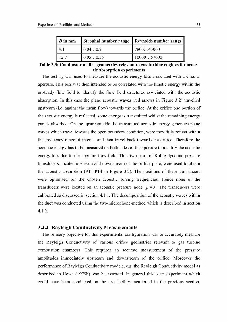
Experimental Facilities and Methods 75
D in mm Strouhal number range Reynolds number range
9.1 0.04…0.2 7800…43000
12.7 0.05…0.55 10000…57000 Table 3.3: Combustor orifice geometries relevant to gas turbine engines for acous-
tic absorption experiments The test rig was used to measure the acoustic energy loss associated with a circular
aperture. This loss was then intended to be correlated with the kinetic energy within the
unsteady flow field to identify the flow field structures associated with the acoustic
absorption. In this case the plane acoustic waves (red arrows in Figure 3.2) travelled
upstream (i.e. against the mean flow) towards the orifice. At the orifice one portion of
the acoustic energy is reflected, some energy is transmitted whilst the remaining energy
part is absorbed. On the upstream side the transmitted acoustic energy generates plane
waves which travel towards the open boundary condition, were they fully reflect within
the frequency range of interest and then travel back towards the orifice. Therefore the
acoustic energy has to be measured on both sides of the aperture to identify the acoustic
energy loss due to the aperture flow field. Thus two pairs of Kulite dynamic pressure
transducers, located upstream and downstream of the orifice plate, were used to obtain
the acoustic absorption (PT1-PT4 in Figure 3.2). The positions of these transducers
were optimised for the chosen acoustic forcing frequencies. Hence none of the
transducers were located on an acoustic pressure node (p’=0). The transducers were
calibrated as discussed in section 4.1.1. The decomposition of the acoustic waves within
the duct was conducted using the two-microphone-method which is described in section
4.1.2.
3.2.2 Rayleigh Conductivity Measurements The primary objective for this experimental configuration was to accurately measure
the Rayleigh Conductivity of various orifice geometries relevant to gas turbine
combustion chambers. This requires an accurate measurement of the pressure
amplitudes immediately upstream and downstream of the orifice. Moreover the
performance of Rayleigh Conductivity models, e.g. the Rayleigh Conductivity model as
described in Howe (1979b), can be assessed. In general this is an experiment which
could have been conducted on the test facility mentioned in the previous section.

Experimental Facilities and Methods 76
However the aim of this experiment was to measure the Rayleigh Conductivity over a
wide Strouhal number range rather than at specific frequencies. This would lead to
reduced accuracy using the two-microphone method (described in section 4.1.2) over a
wide frequency band (e.g. 20 to 1000 Hz). Hence a multi-microphone method
(described in section 4.1.3) would have to be applied to accurately measure the pressure
amplitudes on the upstream and downstream side of the orifice. This would generate a
significant cost as the amount of dynamic pressure transducers would be doubled.
A more cost effective approach was to modify the test configuration as shown in
Figure 3.5. In this case the fan was used to blow air through the test rig as indicated by
the blue arrows. The duct geometry upstream of the orifice was unchanged but for this
setup the test rig was terminated immediately downstream of the orifice test specimen.
Therefore the sound was able to radiate into the surrounding plenum. Thus it can be
assumed that the pressure oscillation immediately downstream of the aperture is zero
for the range of excitation frequencies investigated. In the upstream duct a multi-
microphone method was used to accurately measure the pressure and velocity
amplitudes in the plane immediately upstream of the orifice. A similar setup is described
in Howe (1979b) and used for the derivation of the analytical Rayleigh Conductivity
model. Hence the measurements undertaken within the linear acoustic absorption
regime can be used to assess the performance of the model developed by Howe (1979b).
However the Rayleigh Conductivity was also measured within the non-linear acoustic
absorption regime.
For this setup the acoustic energy loss cannot be directly measured as the transmitted
energy into the plenum was not captured. However the acoustic loss generated by the
apertures can be inferred using the measured admittance and pressure amplitudes on the
upstream side of the orifice using equation (2.43).
The air flow through the test rig was chosen so that the pressure drop (dp/p) across the
orifice was set to 0.5%. The pressure downstream of the test specimen was ambient and
the upstream pressure was measured using a static pressure tapping within the duct prior
to the orifice. Moreover the frequency was varied in increments of 20 Hz from 20 to
1000 Hz. These conditions correspond to a Strouhal number range of 0.02-1.6. At the
maximum frequency of 1000 Hz it is still valid to assume plane axial waves within the

Experimental Facilities and Methods 77
rectangular test section. As already discussed radial modes are expected to cut on at
approximately 1400 Hz. The pressure amplitude for the tests within the linear
absorption regime was set to 130 dB for the plane wave incident onto the test specimen,
for the non-linear acoustic absorption regime the pressure amplitude being increased to
145 dB.
PT1
PT4
PT2
PT3
x = 0
477
763
882
951
Test specimen
Loudspeaker
Section A-A’
120
120
20
4075
A A’
Figure 3.5: Schematic of the test facility for Rayleigh Conductivity measurements, dimensions in mm not to scale
To derive the Rayleigh Conductivity the impedance was measured just upstream of
the orifice (x = 0 Figure 3.5). During the commissioning phase of the experimental
facility the effects of the acoustic radiation upon the impedance measurements have
been assessed. The aim was to ensure the radiation of acoustic energy does not affect
the resistance measurements, since the radiation and inertia effects will be contained in
the reactance of the impedance. However the influence of radiation upon these
measurements is small and is discussed further in chapter 5.4.
Using this approach various test specimens have been investigated that are relevant to
the gas turbine combustion system design envelope. The investigated geometries are
defined in appendix A.2.

Experimental Facilities and Methods 78
3.3 Experiments on Combustion System Representative Acoustic
Damper Geometries In this section test facilities used for the experimental assessment of gas turbine
representative acoustic dampers are introduced. This included
• a facility in which a multi-aperture perforated liner could be incorporated, the
size of which was broadly representative of that found for a single sector of a
full annular combustion system,
• a facility which simulated a single sector of a combustion system including the
fuel injector and associated flow field.
3.3.1 Experiments of Combustion System Representative Acoustic Liners (No Influence of the Fuel Injector Flow Field)
The objective for this test rig was to validate design tools and acoustic absorption
models for perforated liners applicable to gas turbine aero combustion systems.
Isothermal tests were conducted at ambient pressure and temperature on the test
configuration described in Figure 3.6. The test rig consists of a 115 mm by 130 mm
rectangular cross-section. This cross-section was representative of a sector of an annular
combustor. The damper cross-sectional area (40.3 mm by 115 mm) is slightly smaller
than the duct area. This was necessary to achieve combustion system representative
porosities at the relevant pressure drop to remain within the cooling envelope of a
modern gas turbine combustor.
Air is drawn through the passive damper (blue arrows Figure 3.6) which consists of a
metering skin, a volume representative of that available within the combustion system
space envelope and a damping skin. The pressure drop across the test section was set to
3% which is representative of a gas turbine combustor wall. The detailed geometry of
the test section is described in appendix A.3.
Two loudspeakers are used to generate a plane wave travelling towards the test
section (red arrows in Figure 3.6). In this case the reflection coefficient was measured.
Although a small amount of acoustic energy can be transmitted through the passive
damper assembly, as a first assumption this transmitted wave is neglected. To ensure
this assumption is valid the metering skin described in Table A.4 was designed with a

Experimental Facilities and Methods 79
small porosity and long apertures with L/D ratio of 16.67. This ensures that the unsteady
velocity amplitude in the metering skin apertures remains small and the acoustic
behaviour of the metering skin is similar to a rigid wall. Hence the difference between
the incident and reflected wave is assumed to be the acoustic energy loss, which was
subsequently used for the validation of the acoustic models.
A A’ Section A-A’
130
115
20
Test Section
PT1
PT240.3
115
Damping skin
B B’
Section B-B’
S PT4
868
Figure 3.6: Schematic of resonating linear damper test facility, dimensions not to
scale The excitation amplitude was of order 135 dB and was therefore mainly in the linear
acoustic absorption regime. The excitation frequencies were 300 to 450 Hz based on the
described Strouhal number and pressure amplitude scaling (section 3.1).
Kulite dynamic pressure transducers were mounted on the test rig as shown in Figure
3.6. Hence the acoustic energy fluxes of the plane waves could be measured using a
multi-microphone method for transducer positions shown. Furthermore a Kulite

Experimental Facilities and Methods 80
transducer was located within the damper cavity. This transducer was used to assess the
unsteady pressure drop across the damping skin and investigate the resonance frequency
of the volume.
3.3.2 Experiments on Acoustic Dampers Exposed to Fuel Injector Flow Field
This experimental facility was developed to assess passive damping systems exposed
to complex fuel injector flow fields. Therefore a test section representative of a single
sector of a full annular gas turbine combustion system including the fuel injector flow
field was developed. The main objectives of this test section were:
• to investigate the space envelope needed for an efficient passive damper,
• to investigate the effects of a complex fuel injector flow field, relevant to gas
turbine combustion systems, impinging on the damper surface,
• to further validate the used acoustic absorption modelling techniques.
The experimental configuration mounted onto the ambient isothermal aero acoustic
facility is shown in Figure 3.7 and is broadly representative of a single sector of a
(simplified) fully annular lean burn combustion system. The following description of
the test rig can also be found in Rupp et. al. (2012). A square cross-section of 120 mm
by 120 mm duct is used with a gas turbine combustion system representative fuel
injector mounted on to the upstream end of a square acrylic duct. The damper section
consists of a width WD and length LD. An aperture of size DD LW ⋅ on one wall of the
duct, immediately downstream of the fuel injector, enables various passive damper
assemblies to be inserted. This simulates the presence of a passive damper in the outer
(or inner) wall of a flame tube. The parameter S represents the separation between the
damping and the metering skin.
Atmospheric air is drawn through the fuel injector and damper assembly (as indicated
by the blue arrows in Figure 3.7), whilst holes and slots within the injector mounting
plate also simulate the presence of a starter film passing over the damper surface. The
presence of the fuel injector and starter films etc are thought to generate a reasonable
isothermal representation of the complex flow field to which the passive damper would

Experimental Facilities and Methods 81
be exposed within an engine environment. Having passed through the test section this
flow then continues down the duct before issuing into a plenum. Typical operating
conditions correspond to a 3% pressure drop (dp/p) across the fuel injector and damper.
A A’ Section A-A’
12012
020
Test Section
PT1
PT2
964
1250
Array of static pressuretappings
PT3,4
Figure 3.7: Schematic of non-resonating linear damper test facility, dimensions in
mm, not to scale The damper as shown in Figure 3.8 consists of two skins or liners and its design
highlights some of the conflicting requirements associated with operating a porous liner
in a gas turbine combustion environment. The relatively high pressure drop across the
flame tube liner indicates potentially high velocities through any orifices (and hence
low Strouhal numbers). To increase the Strouhal number to a point where, as indicated
by Howe (1979b), some acoustic absorption will take place would require orifices of
relatively large diameter. However, this would result in an unacceptably high flow rate
for the combustion system. Consequently the passive damper consists of two skins in
which the outermost liner is the metering skin. As its name suggests this meters or
controls the flow through the damper and hence most of the mean pressure drop occurs
across this skin. In this case the metering skin pressure drop is set to ~2.7% dp/p. Hence

Experimental Facilities and Methods 82
the remaining pressure drop across the damping skin is set to ~0.3% dp/p. A large
number of small diameter holes can be used to obtain appreciable acoustic absorption.
However, it should be acknowledged there is a compromise between the amount of bias
flow available, the need to keep the liner cool and the amount of acoustic absorption
that can be achieved. The porosities and definition of the damping and metering skin are
defined in appendix A.3.
S
Metering Skin
Damping Skin
H
L D
Fuel Injector
Figure 3.8: Schematic of non-resonating damper test section, not to scale
The acoustic test conditions were chosen to be representative of those conditions
likely to be of interest at engine conditions (when appropriately scaled). In this case the
diameters of the aperture remains of the same size as for the engine. Hence acoustic
frequencies were in the range of 250 Hz to 350 Hz using engine Strouhal number
scaling (equation ( 3.1)). Therefore the acoustic forcing frequencies are well below the
cut-on frequency associated with any higher order duct modes (~1400 Hz). The
excitation amplitudes were set to 135 dB. This was based on the amplitude scaling
applied for the experiments relative to gas turbine combustors (section 3.1).
The complex flow field along the damping skin generated by the fuel injector and the
starter film was assessed using an array of static pressure tappings on the opposite side
of the damping skin as indicated in Figure 3.7. In this case an array of 3 by 4 static
pressure tappings was used along the width and the length of the damper connected to a
set of Furnace FCO 330 pressure transducers.

Experimental Facilities and Methods 83
Not only is the flow field more complex for this test section but the acoustic system is
also more complex. Two Kulite dynamic pressure transducers were used to measure the
acoustic waves within the flow duct using the two-microphone method. The positions of
the pressure transducers have been optimised for the frequency range of interest (PT1
and PT2 in Figure 3.7). Moreover two more Kulite transducers have been used to assess
the pressure amplitudes in the cavity between the metering and damping skins (PT3 and
PT4 in Figure 3.7). However, due to space constraints this was only possible for those
tests with larger spacing between the liners ( 30.≥HS ). As Figure 3.8 indicates the
incident plane acoustic wave (red arrows represent plane acoustic waves) onto the test
section is partly reflected back, part of the wave is transmitted through the fuel injector,
part of the wave is transmitted through the damper and finally some of the acoustic
energy will be absorbed. Only a qualitative assessment can be conducted, which is
based on the change in reflection coefficient due to the change in liner separation SD.
However in later chapters of this work a methodology is developed which allows the
discrimination of the acoustic loss from the transmission of acoustic energy through the
injector.

Instrumentation and Data Reduction 84
4 Instrumentation and Data Reduction In this chapter the experimental methods and data reduction techniques will be
discussed along with an assessment of the experimental accuracies. Initially the acoustic
instrumentation and associated analysis methods will be introduced, followed by the
particle image velocimetry methods used to capture the unsteady flow field.
4.1 Acoustic Measurements The acoustic measurements have been conducted using four miniature high sensitivity
Kulite XCS-093 dynamic pressure transducers. Within this work the sensors will be
referred to as Kulite transducers. A National Instruments LabView data acquisition
system was used as described in Barker et. al. (2005). The acquisition system is outlined
in Figure 4.1. The supply voltage of 10Vdc is supplied by a SCXI- 1520 strain gauge
module. Furthermore the Kulite signal output was conditioned by a SCXI-1143 module.
The temperature within the test rig was measured using a K-Type thermocouple
connected to the SCXI-1112 module which was also within the SCXI-1000 chassis.
Finally the data was acquired using a PC equipped with a National Instruments
LabView PCI-6052E data acquisition card with a 16 bit range for the discretisation of
the analogue signal.
Kulite dynamic pressure transducers
SCXI-1143Module
SCXI-1520Module
SCXI-1112Module
10Vdc Supply
Thermocouple
PCI-6052E
SCXI – 1000Chassis
PC
Figure 4.1: Dynamic data acquisition setup, from Barker et. al. (2005)

Instrumentation and Data Reduction 85
The sampling frequency of the data acquisition system was set up to 40 kHz.
Moreover the pressure signal was sampled using eight blocks of 215 samples, resulting
in a time window of 0.8192 s per data block. Each of the time histories has been Fourier
transformed using the Fast Fourier Transformation method with a Hamming window.
Thereafter an ensemble average over the eight time histories has been conducted on
the Fourier transformed amplitudes:
( ) ∑=
=N
1nn,ii p
N1
fp . ( 4.1)
In this case the subscript i represents the Kulite transducer number (i.e. i= 1, 2, 3, 4) and
n is the time history number (i.e. n = 1,2,…,8). Moreover the parameter N represents the
total amount of time histories N = 8.
The auto power spectra of each transducer signal can then be calculated using the
averaged Fourier transformed pressure amplitudes (Lynn (1989))
( ) ( ) ( )fpfpfS *iiii = . ( 4.2)
Furthermore, one of the signals (Kulite 1) is chosen as a reference to which the other
signals can be compared. For example the cross-power spectrum relative to the
reference signal (Kulite 1)
( ) ( ) ( ),fpfpfS *i1i1 = ( 4.3)
can be calculated, using subscript i to denote the transducer number. Finally the
frequency response functions have been calculated using the auto- and cross-power
spectra (Lynn (1989)):
( )( )( )
4,3,2i,fS
fSfH
11
i1i1 == . ( 4.4)
Hence the measured complex amplitude of each transducer relative to the reference
transducer could be calculated:
( ) ( )fS2fp 111 = and ( 4.5)
Instrumentation and Data Reduction 86
( ) ( ) ( )fHfS2fp i111i = . ( 4.6)
This relates each amplitude measurement in magnitude and phase relative to the
reference transducer which is needed for the two-microphone and multi-microphone
method introduced in sections 4.1.3 and 4.1.4.
4.1.1 Dynamic Pressure Transducer Calibration For the static calibration of the Kulite dynamic pressure sensors a cylindrical vessel
was used. All four transducers have been connected to the vessel. Moreover two
calibrated reference pressure transducers (Furnace Controls differential pressure
transducer Model 332 with an accuracy of 0.5% and a Furnace FC0510 Micro-
Manometer with an accuracy of 0.1%) were also connected to the same vessel. The
static pressure inside the vessel was set using a pump connected to the volume which
pressurised and evacuated the volume over the range -5000 Pa to +5000 Pa. In this way
the static pressure and the output voltage from the Kulite transducers was measured.
Figure 4.2 shows an example of a static calibration curve representative for all four
dynamic pressure transducers. It can be seen that over the range tested the transducer
follows a linear curve with the same slope for negative as well as positive static
pressure. The slopes of the curves are then used to convert the voltage to pressure
signals within the data acquisition system. This static calibration has been conducted at
regular intervals and the sensitivities always remained within 1%.
The dynamic pressure transducers have also been calibrated in terms of their
fluctuating magnitude and phase relationship relative to each other. This is particularly
important for the analysis using the two-microphone and the multi-microphone method.
Therefore the dynamic calibration of the Kulite transducers has been conducted using
the acoustic test rig shown in Figure 4.3, which is basically an open ended duct with
loudspeakers attached. Four Kulite transducers have been mounted at the same axial
position within the duct of cross-section 120 by 120 mm. On each side of the duct a
dynamic pressure transducer is centrally mounted as shown on view B-B’ in Figure 4.3.
Both sides of the test rig were open to atmosphere. Two loudspeakers, as described in
the previous sections, have been used to generate plane acoustic waves (red arrows in
Figure 4.3). The plane acoustic waves only change their amplitude in the axial direction.

Instrumentation and Data Reduction 87
Hence all four dynamic pressure transducers should measure the same pressure
amplitude with the same phase as they are mounted at the same axial plane.
-20000
-15000
-10000
-5000
0
5000
10000
15000
20000
-6000 -4000 -2000 0 2000 4000 6000
Volta
ge in
uV
Pressure in Pa Figure 4.2: Example of static calibration curve
Axial PT location
x = 0
748
Loudspeaker
Section A-A’
120
120
20
A A’
B B’
60 PT1
PT2
PT3
PT4Section B-B’
Plenum
Plenum Figure 4.3: Test rig for dynamic Kulite calibration
The dynamic calibration has been conducted over a relevant frequency range (from 62
to 1000 Hz). The pressure signals have been acquired and the relative complex
amplitudes of the transducers have been calculated as described in section ( 4.1).

Instrumentation and Data Reduction 88
The relative variation in magnitude between the four transducers was investigated
using the average magnitude
4
p
p
4
1ii∑
== ( 4.7)
of the four transducers and the standard deviation of each transducer( Montgomery and
Runger (1994)):
( )14
pp4
1i
2i
p −
−
=∑=σ .
( 4.8)
Thus deviation of the magnitude of each transducer relative to the average signal could
be calculated:
pp
ipσ
ε = . ( 4.9)
This deviation is shown in Figure 4.4. It can be seen that the variation in magnitude,
relative to the average, is below 1% for frequencies which are not in the vicinity of a
pressure node, i.e. pressure amplitude is equal to zero. In the vicinity of a pressure node
this error is larger due to the significant reduction in signal to noise ratio. However, this
is due to the mode shapes of the calibration rig and can be neglected as the transducers
are not normally placed in the vicinity of such pressure nodes.
The phase difference relative to Kulite 1 is shown in Figure 4.5. It can be seen that
there is a negligible phase difference between Kulite 1 and Kulite 2. However, there is a
linear increase in phase difference with excitation frequency for Kulites 3 and 4 relative
to Kulite 1. This is related to a constant time delay associated with the multiplexer data
acquisition card. The card does not sample all four channels simultaneously and a
constant time delay is applied between the sampling of the channels. This leads to an
increase in sampling time relative to the channel number, i.e. channel 2 will have the
smallest phase difference and channel 4 has the largest. This phase change is constant
and therefore a phase correction within the data reduction routine can be applied using a
constant time delay based on the slope of the phase with respect to the frequency.

Instrumentation and Data Reduction 89
0%
1%
2%
3%
4%
5%
6%
7%
8%
9%
10%
0 200 400 600 800 1000
Stan
dard
dev
iatio
n
Frequency in Hz Figure 4.4: Deviation of measured amplitude from mean amplitude for all four
Kulites
-1
0
1
2
3
4
5
6
7
0 200 400 600 800 1000
Phas
e di
ffere
nce
to K
ulite
1 in
deg
rees
Frequency in Hz
Kulite 2
Kulite 3
Kulite 4
Figure 4.5: Phase difference relative to Kulite 1
Figure 4.6 shows the corrected phase using the gradient of the phase difference shown
in Figure 4.5. Note outliers which do not follow the linear curve are also caused by the
vicinity of a pressure node for the measurement and can therefore be neglected. The
phase correction leads to phase differences between the Kulite channels of -0.3° to 0.3°
which are acceptable for the measurements.

Instrumentation and Data Reduction 90
-1.0
-0.8
-0.6
-0.4
-0.2
0.0
0.2
0.4
0.6
0.8
1.0
0 200 400 600 800 1000
Phas
e di
ffere
nce
to K
ulite
1 in
deg
rees
Frequency in Hz
Kulite 2
Kulite 3
Kulite 4
Figure 4.6: Phase correction after calibration relative to Kulite 1
4.1.2 Two Microphone Method Figure 4.7 shows a schematic which is used to describe the two microphone method
in this section. A plane wave is generated by a loudspeaker and travels towards a test
specimen. This is referenced to as the incident wave which has a pressure amplitude ip .
At the test specimen, which could also be an acoustic boundary condition such as a
closed or open end, a portion of the incident wave energy is reflected ( rp ). Hence the
acoustic pressure ( )xp at any point within the duct is a superposition of the incident and
reflected pressure wave:
( ) ( ) ( )xiktiexppxiktiexpptiexp)x(p ri −+ ++−= RRR . ( 4.10)
As discussed in the previous chapter this is also the solution of the wave equation for
plane, one dimensional acoustic waves. Seybert and Ross (1977) proposed a
decomposition of the upstream and downstream travelling wave components if two
microphones at two positions x along the duct are used:
( ) ( )1r1i11 xikexppxikexpp)x(p −+ +−= , ( 4.11)
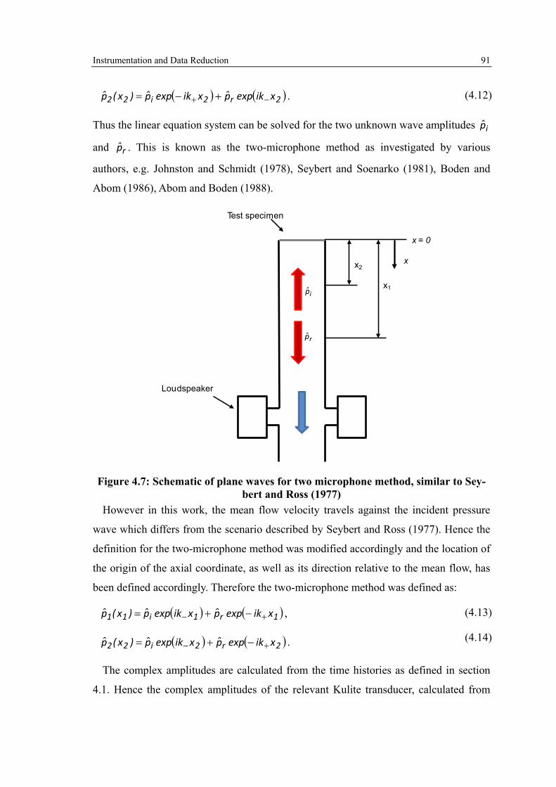
Instrumentation and Data Reduction 91
( ) ( )2r2i22 xikexppxikexpp)x(p −+ +−= . ( 4.12)
Thus the linear equation system can be solved for the two unknown wave amplitudes ip
and rp . This is known as the two-microphone method as investigated by various
authors, e.g. Johnston and Schmidt (1978), Seybert and Soenarko (1981), Boden and
Abom (1986), Abom and Boden (1988).
x = 0
Loudspeaker
ip
rp
x2
x1
x
Test specimen
Figure 4.7: Schematic of plane waves for two microphone method, similar to Sey-bert and Ross (1977)
However in this work, the mean flow velocity travels against the incident pressure
wave which differs from the scenario described by Seybert and Ross (1977). Hence the
definition for the two-microphone method was modified accordingly and the location of
the origin of the axial coordinate, as well as its direction relative to the mean flow, has
been defined accordingly. Therefore the two-microphone method was defined as:
( ) ( )1r1i11 xikexppxikexpp)x(p +− −+= ,
( ) ( )2r2i22 xikexppxikexpp)x(p +− −+= .
( 4.13)
( 4.14)
The complex amplitudes are calculated from the time histories as defined in section
4.1. Hence the complex amplitudes of the relevant Kulite transducer, calculated from

Instrumentation and Data Reduction 92
equation ( 4.5) and ( 4.6), will be used for the measured amplitudes ( )11 xp and ( )22 xp .
Thereafter the incident and reflected wave amplitude can be calculated:
( ) ( )
−−
−
−−−= ++
22
21
222111i
M1
xc
2iexpM1
xc
2iexp
xikexp)x(pxikexp)x(pp
RR,
( ) ( )
−−
−
−−−= −−
22
21
222111r
M1
xc
2iexpM1
xc
2iexp
xikexp)x(pxikexp)x(pp
RR.
( 4.15)
( 4.16)
In general the accuracy of the two micro-phone method is strongly dependent on the
position of the pressure transducers. Seybert and Soenarko (1981) report large errors if
the microphone is positioned at a pressure node due to the poor signal to noise ratio.
Moreover large errors occur if the microphone spacing is exactly half a wave length. In
this case the two equations used for the two microphone method are not linearly
independent (Abom and Boden (1988)). Hence spacing of half a wave length was
avoided. Error estimations on the two microphone method are discussed in section
4.1.4.
4.1.3 Multi-Microphone Method The measurement of the Rayleigh Conductivity described in section 3.1.2 was carried
out over a wide frequency range. Therefore using the two microphone method at fixed
measurement locations would have caused unacceptable errors in the impedance
measurement and therefore in the calculation of the Rayleigh Conductivity. This is due
to the positioning of the dynamic pressure transducers relative to a pressure node within
the duct at certain frequencies. Hence a multi-microphone method was used (e.g.
Poinsot et. al. (1986), Paschereit et. al. (2002), Schuermans (2003)).
In this case four dynamic pressure transducers have been used. Therefore the over
determined linear equation system bAx = can be formed:

Instrumentation and Data Reduction 93
( )
( )
( )
( ) )()
))))) ()))))
b44
11
xr
i
A4
1
4
1
)x(p
)x(p
pp
xikexp
xikexp
xikexp
xikexp
=
−
−
−
−
+
+.
( 4.17)
A least square fit can be used to solve the over determined system whilst minimising the
square of the residual:
22 Axbr −= . ( 4.18)
The tolerance on the residual was set to 10-6, which is the default tolerance in the used
MATLAB routine. In this case the calculation of the wave amplitudes is less prone to
errors as its estimation is dependent on multiple transducer measurement positions.
4.1.4 Error Analysis of Acoustic Measurements In this section error estimates for the acoustic measurements will be discussed. An
analogue input signal to the loudspeakers was generated by a Black Star Jupiter 2010
function generator which was accurate to within 0.1 Hz. The measured excitation
frequency, using the described LabView data acquisition system, did indicate the
forcing amplitudes within 0.1 Hz during the monitoring of the pressure amplitudes (i.e.
in agreement with the function generator). Hence the acoustic forcing frequency was
accurate to potentially 0.1 Hz.
However the signal has been acquired and stored with a 40 kHz sampling frequency
in eight blocks of 215 samples, as described previously. The acquired data has been
Fourier transformed and the absorption coefficient and acoustic losses have been
calculated using a MATLAB routine. Due to the discretisation of the signal the FFT
frequency resolution, or the frequency bin width, was 1.22 Hz. Hence the error on the
frequency was within 0.4 Hz, which is a systematic error in the analysis. The error on
the amplitude of the measured signal is dependent on the position of the acoustic
frequency relative to the centre of the FFT frequency bin width. Therefore a synthetic
signal, similar to the measured pressure signal was used to assess the error due to the
FFT analysis. Figure 4.8 shows the four time traces of the generated artificial signals.
The amplitudes and phase shifts where chosen to be representative of the measured

Instrumentation and Data Reduction 94
pressure signals for the four transducers. Moreover the random noise influence was in
the same order of magnitude. It can be seen from Figure 4.9 that the synthetic signals
represent the random noise as well as other periodic features within the measured
pressure spectra with reasonable similarity.
-200
-150
-100
-50
0
50
100
150
200
0 0.01 0.02 0.03 0.04 0.05 0.06
Ampl
itude
in P
a
Time in s
Signal 1
Signal 2
Signal 3
Signal 4
Figure 4.8: Artificial data set to assess discretisation and FFT accuracy In this case the investigated error on the FFT output was conducted for a 62.5 Hz
forcing frequency. All the measured absorption coefficients where within 0.1 Hz of 62.5
Hz and 125 Hz so the actual forcing frequencies for the synthetic test signals are
representative of the measured frequencies within the acoustic experiments. The
pressure amplitude of the input signal was known, hence the magnitude and phase of the
Fourier transformed signals could be assessed. The error on the magnitude was
calculated as
S,i
S,iFFT,ii,p p
pp −=ε , ( 4.19)
where i = 1, 2 ,3, 4 denotes the synthetic signal of each simulated transducer and the
subscript s denotes the synthetic signal input, whereas the subscript FFT represents the
output of the Fourier transformation. The same can be conducted for the phase
difference between the input to the method and the output out of the routine:

Instrumentation and Data Reduction 95
S,iFFT,ii, ϕϕεϕ −= . ( 4.20)
0 250 500 750 1000
Ampl
itude
in P
a
Frequency in Hz
100
10-3
103
102
101
10-2
10-1
Measured pressure spectrum Kulite 1
0 250 500 750 1000
Ampl
itude
in P
aFrequency in Hz
100
10-3
103
102
101
10-2
10-1
Synthetic signal 1 simulating Kulite 1
0 250 500 750 1000
Ampl
itude
in P
a
Frequency in Hz
10-2
101
100
10-1
10-4
10-3
Measured pressure spectrum Kulite 3
0 250 500 750 1000
Ampl
itude
in P
a
Frequency in Hz
10-2
101
100
10-1
10-4
10-3
Synthetic signal 3 simulating Kulite 3
Figure 4.9: Comparison of synthetic signal and measured pressure signals Thus for the 62.5 Hz excitation frequency the error on the magnitude was 3% and the
maximum error on the phase was 0.02°. As already mentioned the deviation on the
magnitude is a bias error which leads to magnitudes which are always 3% smaller than
the input signal. However the error on the phase of the signal was a random error due to
the artificial noise on the test signal. Thus the complex wave amplitudes, ip and rp , are
affected by the same error in magnitude and a negligible random error in phase.
However the absorption coefficient and the conductivity are less affected by the bias

Instrumentation and Data Reduction 96
error as these quantities are ratios of wave amplitudes relative to each other (and
therefore the bias error reduces). Hence the bias error estimate on the absorption
coefficient reduces to 0.5% whilst the bias error on the conductivity measurement is
estimated to 0.9%. However another important quantity to validate the PIV
methodology is the loss of acoustic energy. This quantity is not normalised and
therefore the bias error will have an effect. In this case the systematic error on the
acoustic energy loss is estimated to 7%.
Some of the acoustic absorption test cases are conducted at an acoustic excitation
frequency of 125Hz. In this case the FFT resolution has been adjusted to 2.44Hz
frequency bin size to reduce the initial bias error on the FFT amplitude to the same level
as described for the 62.5Hz test cases. For all other measurements within this work the
bias error is less important as the calculated quantities are normalised and thus this
systematic error cancels out.
In addition to the bias error on the calculated quantities being estimated, the random
error on the measured pressure amplitudes was also approximated. The variation of the
calculated pressure amplitudes was investigated using the standard deviation between
the single events and the calculated mean pressure amplitude of each of the 8 blocks of
dynamic data from a representative test point at 62.5 Hz forcing and a mean pressure
drop across the orifice of 0.5% dp/p:
( )18
pp8
1n
2in,i
ip −
−
=∑=
σ ,
( 4.21)
where the average magnitude of the pressure amplitude is calculated as:
8
p
p
8
1nn,i
i
∑== .
( 4.22)
Therefore the random error on the pressure amplitude was calculated to
%3.0pi
random,ip == σ
ε . ( 4.23)

Instrumentation and Data Reduction 97
With the same procedure the random phase error of each transducer can be estimated as
no larger than 160.± °. Hence the total random error in the transducer magnitude is of
order %3.1± and the total error in phase is of order 460.± ° including the random
variation as shown in the dynamic calibration (section 4.1.1).
It is also necessary to investigate the error analysis of the two microphone method. In
this case the transducer position has the biggest influence on the size of the error. As can
be seen in Seybert and Soenarko (1981) or Boden and Abom (1985) the largest bias
errors are present if the pressure transducers are located at the pressure node or anti-
node. For the acoustic absorption measurements the error due to the upstream pressure
transducers can be neglected in this setup. The acoustic energy transmitted into the
upstream duct is two orders of magnitude smaller than the acoustic absorption
coefficient. Hence the error influence onto the upstream transducer pair can be
neglected.
Therefore the total error estimates for the acoustic quantities within the two
microphone method are shown in Table 4.1.
Pressure amplitude
Wave am-plitude
Acoustic loss Absorption coefficient
Magnitude 3.3% 3.3% 7% 1%
Phase 0.46 0.46 Table 4.1: Maximum error estimates for quantities calculated with the two micro-
phone method The absorption coefficient of a datum orifice plate has been repeated several times
during the programme and the repeatability of the measurement was within 1%. As the
bias errors cancels for these parameters it was assumed that the random error is the only
influence on the measurement of the absorption coefficient. Thus the maximum error
estimate for the absorption coefficient is %1± .
Placing microphones at locations of pressure nodes and anti-nodes has to be avoided
for the two-microphone method due to the occurrence of large errors within the
measurement. However for the measurement of the Rayleigh Conductivity in this work
a wide frequency range was needed to investigate a wide range of Strouhal numbers.
Therefore pressure anti-nodes and nodes cannot be avoided without a great deal of

Instrumentation and Data Reduction 98
effort in shifting the microphone positions around for given frequency ranges. A more
convenient way to improve the measurement accuracy for this case is the use of a multi-
microphone method as described earlier. Thus errors introduced by transducers at
pressure nodes or anti-nodes are not as influential for the multi-microphone method.
Therefore it can be assumed that the worst case scenario of this method is the accuracy
of the two-microphone method. Hence the maximum errors for the investigated
parameters are as described previously in Table 4.1.
4.2 High Speed PIV Method The velocity field upstream and downstream of the orifice during acoustic excitation
was measured using high speed particle image velocimetry (PIV). This section will give
a brief overview of the method and describe the optimisation of the PIV setup. More
detailed explanation and description of the capabilities of the PIV method can be found
for example in Adrian (1991), Westerweel (1997), Raffel et. al. (2007), Adrian (2005),
Hollis (2004), Robinson (2009), etc. A general arrangement of a PIV measurement
system is shown in Figure 4.10. The setup consists of a laser, digital CCD (charged
coupled device) camera and tracer particles which are seeded into the flow field. The
laser fires two distinct pulses at a given time distance Δt which is known as the inter-
frame time. A divergent lens is used to generate a light sheet from the small circular
laser beam, which illuminates the flow area of interest. Thus the tracer particles within
the light sheet are illuminated and the scattered light is recorded by the digital camera.
Thereby two images, separated by Δt, are generated and the velocity field can be
calculated by measuring the displacement of the particles in the two images and the
inter-frame time Δt:
( )t
)t,x(xt,xu
∆∆
= . ( 4.24)
In this case PIV is a planar measurement technique, hence the velocity is a vector in
the Cartesian (x, y)-plane. The quality of the PIV data acquisition process is strongly
influenced by the choice of: tracer particles, flow illumination, optical setup for the
recording of the images as well as the time synchronisation of the PIV system (e.g.
Hollis (2004)). The optimisation of the PIV system parameters has been conducted

Instrumentation and Data Reduction 99
based on the procedure outlined in Hollis (2004). The main parameters used for the PIV
measurements are summarised in Table 4.2. Particle image velocimetry has been widely
applied in the past to measure the unsteady velocity field of various engineering
applications. Hence this is a rather well established technique. However, a brief
overview of the main components of the PIV measurement technique is discussed in the
following paragraphs.
LASER
High speed camera
Figure 4.10: Schematic of a PIV setup to measure the flow field downstream of an orifice plate
For the illumination of the flow field a Quantronix Darwin-Duo 527-80-M laser has
been used. The laser can generate two pulses of laser light with a repetition rate of 0.1 to
10 kHz. More detailed information about the laser can be found in LaVision (2011). The
illuminated flow field was recorded by a LaVision High Speed Star 5 camera containing
a CCD array with 1024x1024 pixels. More detailed information about CCD- arrays can
be found in Hollis (2004) or Raffel et. al. (2007). A Sigma 105 mm focal length lens
was used with a range of f-numbers of 22f8.2 # ≤≤ . The f-number is defined by the
ratio of focal length to aperture diameter of the lens. The main objective of the optical
setup is to optimise the particle image diameter while ensuring an adequate field of
view (FOV), which is the area of interest within the flow field, for the PIV
measurement. To optimise the optical setup several parameters must be considered:
seeding particle diameter, magnification of the optical setup, the diffraction limited
diameter, size of the CCD array, the wavelength of the laser light and the f-number of
the lens. Guidance in how to optimise the rather complex system can be found in Hollis

Instrumentation and Data Reduction 100
(2004) or Raffel et. al. (2007). In this case the optimisation resulted in a field of view
size of 30x30 mm.
Illumination
Quantronix Darwin Duo 527-80-M Laser rod consists of Yttrium Lithium Fluoride crystal incorporating Neodym ions (Nd:YLF), wavelength 527nm, 1kHz repetition rate
LaVision laser guiding arm -10 mm focal length, light sheet thickness approx. 1mm
Camera and optical setup
LaVision High Speed Star 5 1024x1024 pixel, 17 μm pixel size, 3072 double images, max sampling time 2.793s
Sigma 105 mm focal length lens f-numbers of 22f8.2 # ≤≤ , field of view (FOV) 30x30 mm
Inter-frame time 6-25µs, depending on mean velocity
Vector field calculation and validation
Software LaVision DaVis 7.2
Processing Initial cell size 64x64, 2 iterations
Final cell size 32x32, 3 iterations
50% overlap leading to 64x64 vectors
2nd order correlation
Validation Remove vectors with Q-ratio < 1.5.
Median vector filter >1.3 standard devia-tion.
Replace vectors with 2nd, 3rd or 4th choice vectors. Interpolate if no vector within 4th choice is found.
Amount of first choice vectors >95% Table 4.2: Summary of used PIV system parameters
The sampling frequency of 1100 Hz was chosen to generate an adequate temporal
resolution for the chosen acoustic excitation frequencies of 62.5 and 125 Hz. Thus 18
images per acoustic cycle could be recorded for 62.5 Hz excitation and 9 images per
acoustic cycle could be captured for 125 Hz acoustic excitation. The inter-frame-time
was chosen so that the particle displacement for the two captured frames was optimised

Instrumentation and Data Reduction 101
such that the mean particle displacement was within a quarter of the interrogation cell
(Kean and Adrian (1990)). Hence the inter-frame time has been changed depending on
the mean velocity through the orifice. More detailed discussions of the inter-frame time
can be found in Hollis (2004) or Midgley (2005).
The next step is to calculate the velocity from the recorded images. This process is
illustrated in Figure 4.11. Frame A and frame B are divided into various interrogation
cells. In this case it is approximated that the particles within an interrogation cell move
homogeneously. A spatial cross-correlation method is used between the particle pattern
of interrogation cells in frame A and frame B with the help of a Fast Fourier
Transformation (FFT) method. The outcome of this correlation is a correlation map
where the average displacement of the particle pattern within the interrogation cell is
indicated by the peak in the correlation map (Figure 4.11). This displacement vector can
then be used to calculate the velocity within the interrogation cell using the inter-frame
time ∆t. A more detailed formulation of the cross-correlation technique can be found for
example in Raffel et. al. (2007).
dx dy
Frame A time t1
Frame B time t2 = t1 + ∆t
Interrogation cell
Interrogation cell
Interrogation cellFrame A and B
Cross-Correlation map
Displacement
xd
Figure 4.11: Cross-correlation to evaluate particle displacement, from LaVision
(2007) A further improvement in the quality of the vector data is to use adaptive multi pass
grids (e.g. Hollis (2004)). In this case the initial cell size was chosen to be 64×64

Instrumentation and Data Reduction 102
pixels. During the first two iterations the vector field was calculated using this cell size.
Thus a first approximation of the vector field was achieved. During the second iteration
the interrogation cells will be shifted according to the previous vector calculation. This
ensures a correlation with the same particles which improves the accuracy of the vector
data and avoids the loss of particles across the cells. Moreover the information is then
used to move the further reduced cells to 32×32 pixels for a further three iterations.
Therefore the advantage of this method is that particles within the smaller cells are not
lost into surrounding cells for the correlation between the image pairs. Thus the
accuracy of the data can be improved (LaVision (2007)).
Finally the quality of the calculated vectors will be checked using various methods
such as
• Q-ratios, which takes the ratio of the maximum peaks in the correlation map into
account,
• median filters, which investigate the surrounding vectors and
• peak locking parameters, which assess the velocity field on its bias to integer
values.
All of these methods have been discussed in detail for example in Westerweel (1994),
Hollis (2004), LaVision (2007). Nevertheless a particularly relevant part for all PIV
measurements is the adequate choice of seeding particles. This will be discussed in
more detailed in the following section.
The described criteria have been used together with the optimisation steps described
in Hollis (2004). This lead to 98% first choice vectors within the non-linear absorption
measurements at close to zero mean pressure drops across the aperture. The first choice
vector percentage was lower in the linear regime as the increased mean jet velocity
results in an increased dynamic range in measured velocity between the jet velocity and
the acoustic velocity in the surrounding duct. Nevertheless a minimum of 95% of first
choice vectors were indicated in DaVis 7.2 for the investigated flow fields.

Instrumentation and Data Reduction 103
4.2.1 Tracer Particles
The seeding particles of the flow field have two main functions in the PIV setup: they
have to follow the flow accurately and they must scatter enough light to be captured by
the camera. Unfortunately these requirements can be in conflict with each other and
require careful optimisation. Westerweel (1997) shows that the minimum error in the
measurement of the particle displacement occurs for a particle image size of
approximately 2 pixels. This optimum pixel diameter can be achieved by the choice of
tracer particles together with the optimisation of the optical parameters, while ensuring
the particles follow the flow field accurately. The latter is even more challenging for an
acoustically forced flow field as the particle has to be able to follow the changes in
direction of the flow due to the acoustic excitation. However in this case it should be
noted that the acoustic wave does not require resolving, rather it is the pulsatile jet flow
that is a result of the acoustic pressure oscillation that must be captured.
The temporal velocity variation of a sphere moving in a fluid at high acceleration but
low velocity can be described by the Basset-Boussinesq-Oseen equation (e.g.
Schoeneborn (1975), Siegel and Plueddemann (1991), etc). Tondast-Navaei (2005) uses
a simplified expression of this equation for the application of seeding particles in an
acoustically excited flow field. The assumptions in Tondast-Navaei (2005) were based
on:
• the spherical particles do not deform and interact with each other,
• the particle diameter is much smaller than the sound wave length,
• the density of the particle is much greater than the density of the air
• the difference in acceleration between the particles relative to the air is small
• the Reynolds number is small so that Stokes law is valid.
Hence the reduced Bassett-Boussinesq-Oseen equation can be defined as:
( )PFpPP
3p uur6v
dtd
3r4
−= µπρπ
. ( 4.25)

Instrumentation and Data Reduction 104
The subscript F denotes the working fluid properties, in this case air, and the subscript P
denotes the particle properties. Tondast-Navaei (2005) rearranged the equation and
introduced the relaxation time
( )νρ
ρτ
2p
F
PPP
r92
r = . ( 4.26)
In this case the relaxation time is dependent on the density ratio between the air and the
seeding particles and the size of the seeding particle. Therefore the larger the particle the
larger the relaxation which is a measure of the response of the particle to changes in
velocity, i.e. accelerations and decelerations of the flow field. This introduces a phase
shift between the particle and the air flow.
( )P1tan Rτϕ −= .
( 4.27)
Using the relaxation time in the differential equation (3.32) leads to the inhomogeneous
differential equation:
FPPP uuudtd
=+τ . ( 4.28)
In the case described by Tondast-Navaei (2005) this equation was then solved for an
acoustic standing wave with the resulting velocity field oscillation
( )tcosxc
sinuF RR
= . ( 4.29)
Thus the resulting particle velocity amplitude was defined as:
( ) ( ) ( ) ( )
−+−=
PFFp
texpsinvtsincosvt,xv
τϕϕRϕ . ( 4.30)
Hence the cosine of the phase angle, Tondast-Navaei (2005) refers to this as
“entrainment coefficient”, can be used as a measure of how accurate the particle will
follow the flow in terms of its amplitude, i.e. for 0→ϕ the particle velocity will be
exactly the same as the velocity of the surrounding air flow. The coefficient was
assessed for the available seeding liquid. For these measurements a SAFEX fog
generator was used with the particle density being of order 3p mkg1000=ρ .

Instrumentation and Data Reduction 105
Moreover the kinematic viscosity of the air at ambient temperature was set to
sm1068.15 26−⋅=ν . Figure 4.12 shows the distribution of the entrainment coefficient
with particle size. It can be seen that that the particle velocity will accurately follow the
flow velocity for particle diameter less than 6 μm.
0
0.2
0.4
0.6
0.8
1
1.2
0 5 10 15 20 25 30 35 40 45 50 55 60
cos(
ϕ)
Particle diameter in µm
Figure 4.12: Entrainment coefficient relative to particle size The droplet size of the SAFEX fog generator was measured by Wigley (2008) using a
Phase Doppler Anemometer (PDA). The droplet size distribution is shown in Figure
4.13 using a probability density function as a measure of the occurrence of the droplet
size within the sample of the PDA measurement. It can be seen that less than 5% of the
droplets are greater than 6 μm diameter. Moreover the majority of the droplet diameters
are in the order of 3.5 μm. Furthermore the Sauter Mean Diameter was measured to 3.7
μm.
Not only is the size of the seeding particles important but also the amount. As already
discussed the PIV method relies on a discretisation of the captured images in several
interrogation windows. According to Raffel et. al. (2007), Hollis (2004) or LaVision
(2007) the amount of particles within an interrogation cell should be greater than five.
In this case the displacement vector detection algorithm for the used software is in the
order of more than 95%.

Instrumentation and Data Reduction 106
0%
5%
10%
15%
20%
25%
30%
35%
40%
45%
50%
0 1 2 3 4 5 6 7 8
Particle Diameter in μm
Figure 4.13: Droplet diameter distribution of SAFEX fog seeder
4.2.2 Error Analysis One of the major influences on the accuracy of the PIV measurement technique is
how well the seeding particles are following the flow field. In this case the velocity field
is forced with an acoustic pressure oscillation. Hence the particles as discussed earlier
had to be chosen so that they are accurately following the fluid velocity field for the
given pressure oscillation. A simple way to estimate the error due to the particle slip
velocity is shown for example in Adrian (1991):
νρρ
F
p2pp
Fp 36ud
uu
=− . ( 4.31)
In this case the surrounding fluid and the seeding particle is represented by the subscript
F and p respectively.
The oscillating velocity field relevant for the particle was estimated to
( ) ( )tsinutu pp R= . ( 4.32)
Hence the particle acceleration can be estimated as

Instrumentation and Data Reduction 107
pp uu R= . ( 4.33)
Therefore the systematic error in velocity amplitude relative to the fluid velocity
amplitude can be estimated
F
Fps,u u
uu −=ε . ( 4.34)
The calculated errors are summarised for the two forcing frequencies in Table 4.3.
Acoustic forcing fre-quency in Hz
Estimated error due to particle slip in %
62.5 0.8
125 1.6 Table 4.3: PIV error estimate due to particle slip velocities
Another source of error is the random error due to the calculation of the particle
displacement within the PIV system analysis algorithm. This error can be estimated to
0.1 pixel (Raffel et. al. (2007)). Thus leading to an accuracy on the oscillating velocity
of 0.5 m/s for the shortest inter-frame times of 6μs for the test points at 0.8% dp/p.
Hence this error can be as high as %5.2r,u =ε for the forced velocity fields within the
centre of the jet.
Therefore the total error on the measured velocity amplitudes within the centre of the
jet flow can be estimated using (Morris (2001)):
%32r,u
2s,ut,u =+= εεε . ( 4.35)
This error can be larger within the shear layer of the jet due to the spatial and temporal
resolution of the measurement technique. Further analysis of errors encountered within
the PIV measurement of the aero-acoustic flow field is discussed in Chapter 7 and
appendix D.

Acoustic Absorption Experiments – Linear Acoustic Absorption 108
5 Acoustic Absorption Experiments – Linear Acoustic Absorption
Over recent years a great deal of research has been undertaken to measure and model
the absorption associated with perforated walls. The current work extends this to orifice
geometries typically found in gas turbine combustors and scaled to the relevant
operating condition. Acoustic absorption experiments have been undertaken to
investigate the relevant absorption mechanisms for these geometries prior to
measurements of the associated unsteady flow fields presented later in this work. The
current section presents the experimental results associated with the linear acoustic
absorption regime. Initially the influence of the mean flow through the aperture, and its
influence upon the acoustic absorption, will be investigated. Thereafter the effect of
combustion system orifice geometries, in terms of their length to diameter ratio for
cylindrical apertures, as well as non-cylindrical orifice shapes, will be considered.
Using this data acoustic absorption models and their performance in comparison with
the linear acoustic experiments are assessed and are also used to explain some of the
experimental results. Finally the amount of linear acoustic absorption available within
gas turbine combustion system geometries and operating conditions is discussed.
5.1 Influence of Mean Flow upon Linear Acoustic Absorption In this case a mean flow through the aperture is applied using the facility described in
section 3.1.1. Some example results can be seen in Figure 5.1 similar to those described
in Rupp et. al. (2010) and Rupp et. al. (2010b). In this case the acoustic absorption
coefficients presented are for orifice plate number 1 (Table A.1) with an aperture
diameter of 12.7 mm and an orifice length of 6 mm. The acoustic excitation frequency
was 125 Hz and the absorption data is presented as a function of the incident pressure
amplitude in dB. Note the dB scale for the data shown in this chapter is based on the
peak pressure amplitude not the rms. It is evident that the absorption levels for the test
cases with a mean pressure drop across the orifice of 0.5% to 2.9% are independent of
the excitation amplitude. Hence this result indicates linear absorption over the range of

Acoustic Absorption Experiments – Linear Acoustic Absorption 109
values tested. It can also be seen that a decrease in the pressure drop, and hence the
mean flow passing through the orifice, results in an increase in absorption coefficient
(Rupp et. al. (2010)).
Figure 5.2 shows the measured acoustic absorption coefficient for orifice plate
number 3, D = 9.1 mm and L/D = 0.5. In this case the acoustic forcing frequency was
chosen to be 62.5 Hz. Again it is observed that the absorption coefficient is independent
of the excitation pressure amplitude and thus the absorption mechanism is linear.
Moreover the absorption is increasing with reducing pressure drop (as seen in Figure
5.1).
Alternatively the absorption shown results can be presented using the acoustic
admittance. The admittance can be calculated from the measured acoustic energy flux
incident onto, and reflected by, the orifice plate (equation (2.27) and (2.28)). This can be
calculated on either side of the orifice within the experimental facility. Hence the
incidental acoustic energy is defined as the energy flux travelling against the flow
direction (-) in the downstream duct (ds) and the energy flux travelling in the flow
direction (+) in the upstream duct (us):
+− Π+Π=Π usdsin . ( 5.1)
Furthermore the acoustic energy reflected off the orifice plate can be calculated using
the acoustic energy flux travelling in the flow direction within the downstream duct and
against the flow direction within the upstream side of the test facility:
+− Π+Π=Π dsusout . ( 5.2)
The acoustic energy loss is then calculated as the difference of the incidental and
reflected acoustic energy:
outinL Π−Π=Π . ( 5.3)
According to Howe (1979b) or Luong et. al. (2005) the acoustic energy loss is defined
as:
ρRδRpp dsusL
2ˆˆ −=Π . ( 5.4)

Acoustic Absorption Experiments – Linear Acoustic Absorption 110
In this case the pressure amplitudes are immediately upstream and downstream of the
orifice. As already described in Chapter 3.2.1 the pressure amplitude upstream of the
orifice is effectively zero, due to a pressure node. Hence the admittance can be
calculated using the measured acoustic energy loss and the measured pressure amplitude
from the two-microphone method immediately downstream of the orifice:
2ds
L
pR ˆ
Rρδ
Π= . ( 5.5)
This has been compared to the admittance defined by Howe (1979b) as shown in
equation (2.40). The analytical admittance is only dependent on the Strouhal number. As
already described in section 2.5.1 the Strouhal number can be defined using the velocity
in the plane of the aperture
DdD CUR
URSt
RR== . ( 5.6)
The discharge coefficient for the two orifice plates was measured as 0.73 using the test
arrangement described in the appendix B.
In a similar way as in Rupp et. al. (2012) Figure 5.3 shows the admittance derived
from the experimental data presented in Figure 5.1 and Figure 5.2 in comparison with
the theoretical admittance as described in Howe (1979b). As can be seen the
measurements are in excellent agreement with the theory for the investigated Strouhal
number range from 0.06 to 0.5. Moreover the admittance is increasing for increasing
Strouhal numbers which, in this case, is caused by a reduction in mean velocity across
the aperture. Thus the increasing admittance with decreasing mean velocity leads to a
larger acoustic energy loss and thus to increasing absorption coefficients as shown in
Figure 5.1 and Figure 5.2.
Comparing the two orifice plates leads to the conclusion that plate 1 (Figure 5.1) is
generally generating larger acoustic absorption coefficients for the same pressure drop
(dp/p = 0.5%) than plate 3 in Figure 5.2. This, to some extent, can be expected as the
Strouhal number is increased for plate number 1 in Figure 5.1 due to the larger orifice
diameter and higher forcing frequency. Hence as it is indicated in Figure 5.3 the

Acoustic Absorption Experiments – Linear Acoustic Absorption 111
admittance of the orifice is increasing over the range of Strouhal numbers (St < 1)
investigated and therefore leads to greater acoustic absorption.
It can be seen from equation ( 5.4) that the ability to absorb acoustic energy by an
orifice is dependent on the unsteady pressure difference, the orifice radius and its
admittance (this being a function of Strouhal number). Hence optimising the absorption
of a passive damping device or the cooling geometry of a gas turbine combustor can be
achieved by (i) maximising the unsteady pressure drop or (ii) the admittance of an
orifice geometry. The unsteady pressure drop can be modified using acoustic cavities,
(i.e. plenum or resonating cavities surrounding the porosities) whilst the admittance is in
general a function of Strouhal number. Hence reducing the mean pressure drop across a
perforated liner (and thereby increasing the Strouhal number) increases the admittance
and ultimately the acoustic absorption of the damper for Strouhal numbers smaller than
one. However, due to cooling reasons within a gas turbine combustion system the mean
pressure drop cannot be reduced by large amounts. Thus typical acoustic damper
geometries within gas turbine combustors operate at Strouhal numbers below 0.3 (Rupp
et. al. (2012)). Furthermore other geometries need to be investigated which affect the
admittance of an orifice. In this work the effects of the orifice geometry, in terms of its
L/D and its shape, upon the linear admittance are investigated for gas turbine
combustion system design applications.
5.2 Reynolds Number Independence Howe (1979b) assumes in his analysis that the Reynolds number is sufficiently high
that the acoustic absorption is independent of the Reynolds number. In this case the
Reynolds number is defined as
νρ DUd=Re
. ( 5.7)
Due to the restrictions on the test facility the experiments could only be conducted
over a limited range of Reynolds numbers. However to ensure that the acoustic
absorption measurements were independent of Reynolds number tests were conducted
using orifice plate geometries 2 and 4 described in Table A.1. The Strouhal number was
kept constant and the Reynolds number doubled for the investigated test conditions.
Acoustic Absorption Experiments – Linear Acoustic Absorption 112
This was achieved by varying the mean flow velocity through the aperture. It can be
seen in Figure 5.4 that the admittance remains constant with varying Reynolds number.
Hence it can be assumed the measured linear absorption characteristics shown in this
section are independent of the mean flow Reynolds number.
5.3 Influence of Orifice Shape on the Linear Acoustic Absorption As already mentioned in chapter 1.3 conventional as well as modern combustion
systems can have a host of orifice geometries for cooling, damping and emissions
control purposes. In general the length-to-diameter ratios of apertures within such a
system ranges by an order of magnitude (i.e. from one to ten). Hence the acoustic
absorption associated with these geometries was also investigated.
Figure 5.5 shows a comparison between two orifice plates of the same diameter 9.1
mm with L/D ratios of 0.5 and 2.4 as defined in Table A.1. The mean pressure drop
across the orifice was 0.8% which is typically used for double skin impingement
effusion cooling geometries. Moreover the forcing frequency was set to 62.5 Hz. The
length-to-diameter ratio of 2.4 is representative of combustion system effusion cooling
geometries. As can be seen the absorption remained within the linear regime for the
investigated excitation pressure amplitudes, i.e. constant absorption coefficients with
increasing pressure amplitudes. Moreover there is an increase of approximately 15% in
absorption coefficient for the larger L/D ratio of 2.4 compared to 0.5. Due to the change
in orifice length-to-diameter ratio the Strouhal number for the same pressure drop has
changed due to the increase in discharge coefficient (equation ( 5.6)), i.e. CD of 0.73 for
L/D = 0.5 and CD of 0.84 for L/D of 2.4. Thus the Strouhal number for an L/D of 2.4 is
lower than for L/D of 0.5. According to the previous section based on the theory by
Howe (1979b), the lower Strouhal number should lead to a reduction in admittance and
ultimately in absorption. To the contrary this was not shown by the experiment as
absorption coefficients increased with reducing Strouhal numbers. Therefore the change
in discharge coefficient seemed to have a beneficial effect upon the absorption of
acoustic energy which also suggests that the admittance curve, relative to the Strouhal
number, must have changed.

Acoustic Absorption Experiments – Linear Acoustic Absorption 113
To investigate this behaviour further Figure 5.6 shows a summary of all absorption
experiments for L/D ratios of 0.5 to 10. In this case the diameters of the orifice plates
have remained constant. Furthermore the pressure drop across the orifice plates has
been varied from 0.1 to 1 % leading to Strouhal numbers of 0.06 to 0.2 (taking the
measured discharge coefficients of the orifice plates into account). First of all it can be
seen that the absorption coefficient increases with reducing pressure drop for all orifice
plates smaller than L/D of 5. For larger orifice plates this has less of an effect. It can be
assumed that large L/D ratios (L/D of five and above) are dominated by inertial forces in
the orifice flow field, as the mass of the fluid within the aperture is becoming
increasingly larger, and thus the absorption coefficients reduce as unsteady velocities
decrease due to the increasing inertial forces. Furthermore boundary layers within the
orifices will start to develop for these geometries which will add to the acoustic
resistance. This increase in resistance will lead to a reduced admittance due the
increased boundary layer viscosity reducing the oscillating velocity field and thus the jet
shear layer interaction. Some interesting behaviour though, can be seen for orifice
length-to-diameter ratios between 0.5 and 5. The absorption seems to increase for L/D
ratios from 0.5 to 2, and then decrease for length-to-diameter ratios larger than two. This
increase and decrease of absorption coefficient is pressure drop dependent though, as
absorption coefficients are dropping for L/D > 1 at dp/p of 0.3 and below.
In general the shape of the absorption coefficients with changing L/D ratio resembles
that of the discharge coefficient variation with L/D ratio (as shown in Figure 5.7). The
discharge coefficients have been measured on the described experimental facility in
appendix B. A comparison of the discharge coefficient measurement for the investigated
length-to-diameter ratios is compared to discharge coefficients found in the literature,
e.g. Lichtarowicz et. al. (1965). The measurement shows the same characteristic as
shown in the literature and is in reasonable agreement with the quantitative values. It
can be seen that the discharge coefficient initially increases from 0.65 < L/D < 2 and
then gradually decreases. As already discussed in chapter 2.1 this is due to attachment
of the flow within the orifice occurring at L/D ratios of approximately two. This
suggests that the increase in discharge coefficient is also causing an increase in the
absorption coefficients. This can also be seen looking into more complicated orifice

Acoustic Absorption Experiments – Linear Acoustic Absorption 114
shapes as defined in Table A.1. Figure 5.8 shows the linear acoustic absorption
measurements for various aperture shapes with respect to its measured discharge
coefficients for a mean pressure drop of 0.5%. All orifice lengths were the same (L = 18
mm). Hence it can be assumed as a first approximation that the inertia effects are of
similar scale for all the apertures in Figure 5.8. In one case, plate number 12, the conical
hole has been tested with two different mean flow directions through the orifice as
indicated in Figure 5.9. All the other apertures shown in the figure have been tested with
the mean flow direction going from the largest diameter to the smallest diameter, as for
the left hand side in Figure 5.9. The experimental data confirms the behaviour seen from
the L/D variation as the acoustic absorption coefficient is increasing with increasing
discharge coefficient. Hence the highest absorption coefficient was achieved using a
Bellmouth shaped inlet and the lowest absorption coefficient is measured for the conical
shape in reverse flow direction which provides the lowest measured discharge
coefficient.
This apparent effect of the discharge coefficient on the acoustic absorption coefficient
suggests that the CD, not only affects the mean flow field through the orifice but also the
unsteady flow field (or more precisely the admittance of the orifice). The edge condition
at which vorticity is shed from the rim of the aperture will be affected by changes in the
orifice flow as reflected by the change in CD. Therefore changes in admittance with
changing CD will be investigated in the following section.
5.4 Influence of Orifice Geometry on the Rayleigh Conductivity The previous section showed the measured absorption coefficient is influenced by the
orifice discharge coefficient, but measurements were over a limited Strouhal number
range. Moreover the changes in CD leading to larger acoustic absorption can only be
explained if the admittance curves relative to the Strouhal numbers have been changed.
Hence an orifice Rayleigh Conductivity experiment has been designed to directly
measure orifice admittance and inertia over a wide range of Strouhal numbers and for a
range of length-to-diameter ratios (0.14 to 10). Note the shorter orifice plates have been
included as the theory presented by Howe (1979b) assumed an infinitesimally thin
orifice plate. The pressure drop across the orifice geometries was kept constant to 0.5%.

Acoustic Absorption Experiments – Linear Acoustic Absorption 115
This was set so that the linear absorption regime was present over a wide range of
excitation pressure amplitudes. Experiments with various pressure amplitudes have
been undertaken to prove the admittance remained constant and thus the measurement
remained in the linear regime. Moreover the excitation frequency was varied between
20 to 1000 Hz to achieve a wide range of Strouhal numbers.
The change in test rig to the facility described in chapter 3.2.2 improved the accuracy
of the Rayleigh Conductivity measurements. As was presented in Figure 3.5 the orifice
plate was located at the origin of the axial coordinate at x = 0. Thus the impedance on
the upstream side of the orifice was measured by calculating the pressure amplitude and
velocity amplitude immediately upstream of the orifice using the described multi-micro-
phone-method (section 4.1.3):
( ) ( ) ( )( )
( )( )0
00
000
==−
==
=−===
xuxp
xuxpxp
xZ ususdsˆˆ
ˆˆˆ
( 5.8)
Note the downstream pressure amplitude was negligible as the orifice outflow side
was open to a large plenum. The Rayleigh Conductivity and the impedance rely on the
accurate measurement of the velocity within the orifice. Hence the velocity amplitude
within the aperture can be calculated by using the impedance from equation ( 5.8) and
the cross-sectional area of the upstream duct (Ap) along with the orifice plate itself (AD):
( )pp
us
DD
usD Au
pAu
pZxZ
ˆˆ
ˆˆ
−=−=== 0 . ( 5.9)
In this case multiple apertures have been placed in the test specimen to improve the
measurement accuracy. Thus the porosity of the orifice plate has to be considered to be
able to reduce the data to a single orifice Conductivity. The porosity is defined as:
Pp
DA
RNAA 2π
σ == . ( 5.10)
For a single orifice the pressure amplitude upstream of the orifice tends to be close to
an anti-node which means that the velocity amplitude is small which can give rise to
large errors. However the error can be reduced by increasing the number of orifices
within the plate. Hence multiple orifice plates of the same geometry and with gas
Acoustic Absorption Experiments – Linear Acoustic Absorption 116
turbine combustion system representative pitch-to-diameter ratios (P/D) have been
optimised to reduce the acoustic wave reflection off the test specimen and thus increase
the velocity amplitude in the vicinity of the orifice plate. In this way the measurement
accuracy is increased. The specification of the tested aperture geometries can be found
in Table A.3.
The Rayleigh Conductivity can then be calculated from the measured quantities as
defined by Howe (1979b):
( )Dus
DR Z
ipu
RiiRK 12 2 RρRρπδ −=−=−Γ=ˆˆ
. ( 5.11)
5.4.1 Orifice Conductivity Test Commissioning Initial commissioning of the test rig has been conducted to estimate the accuracy of
the experimental facility. Sun et. al. (2002) used a similar test facility to investigate the
effect of grazing flow on the acoustic impedance of an orifice plate. The authors
proposed to measure the acoustic reactance at low amplitude and with no mean flow
through the apertures to understand how representative the experimental data is
compared to reactance data in the literature. The same methodology has been adopted
during the commissioning phase of the experiments in this work. For low amplitude
acoustic forcing the acoustic reactance is defined as (e.g. Ingard and Ising (1967) or Sun
et. al. (2002)):
( ) ( )σ
Rσ
Rρ
RLc
L
ccX
Z effZD
71.Im
+=== ( 5.12)
This approach is based on the experimental data shown in Ingard and Ising (1967) in
the low amplitude forcing regime without the influence of mean flow. In this case it can
be seen that the acoustic reactance of an aperture is constant and the effective length is
equal to RLLeff ⋅⋅+= 8502 . .
An example of the measured reactance compared to the theoretical values for the
range of frequencies between 50 to 1000 Hz is shown in Figure 5.10. This is an example
representative of all the investigated orifice plate geometries. Sun et. al. (2002)
compared the gradient of the theoretical curve with the measured data and found a
Acoustic Absorption Experiments – Linear Acoustic Absorption 117
variation in gradient no worse than 4.1%. For the orifice plates investigated in this work
the variation in the gradient of the reactance measurement relative to the literature
values was less than 5%. This was used as a criterion to optimise the experiment in
terms of the amount of apertures in an orifice plate and the maximum forcing frequency.
Thus for longer orifice plates with higher L/D ratios the excitation frequency was
reduced to a maximum of 600 Hz. Higher frequency would have resulted in larger
deviations because the assumption that the orifice is short relative to the acoustic wave
length ( L>>λ ) is no longer valid.
The impedance (or Rayleigh Conductivity) of an aperture needs to take the acoustic
radiation of the orifice flow field into account as well (e.g. Ingard and Ising (1967)).
This additional radiation impedance is generated by the aperture flow field analogous to
a solid piston representative of the orifice diameter and length. Hence the oscillating
orifice flow is also a source of sound radiation. This radiation is split into a resistive and
reactive component (e.g. Cummings and Eversman (1983):
( ))())() cereac
eff
ceresi
rad LiRk
cZ
tantan
Rρρ +≈4
20 . ( 5.13)
As can be seen from equation ( 5.13) the reactance is already accounted for in the
measurement in terms of the length correction representing the forces due to the fluid
acceleration of the orifice flow field. In general the radiation resistance can be neglected
as it is very small for the orifice diameters investigated. This is shown in Figure 5.11 for
the measured resistance (note in this case the orifice impedance is defined as DupZ ˆˆ= )
and the theoretical radiation resistance (equation ( 5.13)) for the measurement with 0.5%
pressure drop and the orifice plate with L/D = 0.5. It can be seen that the measured
resistance is much larger than the radiation resistance for the majority of the
measurement and hence the radiation effects in the resistance term is neglected for the
geometries tested.
5.4.2 Orifice Conductivity Test Results The measured Rayleigh Conductivity for the orifice plate with L/D = 0.5 (Plate 20 in
Table A.3) is shown in Figure 5.12. It can be seen that the admittance increases from 0

Acoustic Absorption Experiments – Linear Acoustic Absorption 118
to approximately 0.6 as the Strouhal number increases from 0 to 0.8. The inertia reaches
its maximum value of 1.0 at a Strouhal number of 1.3. After the admittance has reached
its maximum a steep reduction in admittance for increasing Strouhal number is visible.
Furthermore the admittance is negative over a Strouhal number range of 1.4 to 1.8. The
change in sign to a negative admittance suggests production of sound instead of
absorption.
Figure 5.13 presents a comparison of the measured Rayleigh Conductivity with the
theoretical conductivity curves as described by Howe (1979b) (equation (2.39) and
(2.40)). The experiment and the theoretical curves are in good agreement up to a
Strouhal number value of 0.8. Thereafter the experiment deviates with the theoretical
curve with no negative admittance being present in the model. However, over the
Strouhal number range of 1.4 to 1.8 it should be noted that a distinct whistling of the jet
flow during the experiment was observed. Testud et. al. (2009) noticed jet whistling
frequencies for a Strouhal number range of 4020 .....== Dj UfLSt . The Strouhal
number in Testud et. al. (2009) was defined using the length of the aperture. Applying
this Strouhal number definition onto the presented data in Figure 5.13 indicates that the
negative admittance occurs for 3020 .....== Dj UfLSt . Hence this is in agreement
with the data presented in Testud et. al. (2009). Therefore this could be a plausible
explanation for the occurrence of the negative admittance as the whistling is a source of
sound energy, and thus more acoustic energy is generated than absorbed leading to a
sign change in admittance.
The whistling of the jet is caused by a self-excited oscillation of the fluid due to the
dynamic shear layer instability, as discussed in section 2.2 (e.g. Crow and Champagne
(1971), Yule (1978), Hussain and Zaman (1981), etc), interacting with the acoustic
excitation. In the work presented by Testud et. al. (2009) the measured whistling
frequencies occur in the mentioned Strouhal number range of 0.2 to 0.4 based on the
length of the aperture. Hence the timescale of the fluid travelling through the aperture,
relative to the time scale of the acoustic excitation, is the relevant phenomena for the
occurrence of the whistling. Nevertheless other parameters such as the length-to-
diameter ratio and the contraction ratio (porosity) of the orifice are also important since
they affect the jet shear layer and hence the potential for flow instabilities.

Acoustic Absorption Experiments – Linear Acoustic Absorption 119
The jet whistling phenomenon is not accounted for in the developed model from
Howe (1979b) Furthermore the whistling of the jet could also explain the change of
inertia in the experiment relative to the model. As described in section 2.2 large vortex
ring structures are generated by shear layer instabilities (e.g. Crow and Champagne
(1971)) which affect the unsteady flow field and which can lead to increased inertia
within the flow field. A similar change in admittance can also be seen in the
measurements of Jing and Sun (2000). Note that changes in the sign of the admittance δ,
i.e. imaginary part of the Rayleigh Conductivity, are also visible as changes in sign of
the resistance, i.e. real part of the impedance. The data shown in Jing and Sun (2000) for
an L/D = 0.6 orifice is changing sign from positive to negative at Strouhal numbers
around 1.39, hence this could also be caused by self-excited jet instabilities. Moreover
the numerical model from Jing and Sun (2000) which includes jet flow profiles and
orifice thickness effects, described in section 2.5, seems to be able to reproduce this
phenomenon to some extent.
Although tests have been conducted over a wide range of operating conditions the
maximum Strouhal number of interest based on orifice radius and the scaling from
engine to test rig is 0.7 (see Table 3.2). The Strouhal number being this large is due to
the large diameter port features within a RQL combustor. Possible aero-engine gas
turbine passive damper geometries, e.g. Rupp et. a. (2012), are based on Strouhal
numbers smaller than 0.3 for combustion instability frequencies below 1000 Hz. In this
case a large amount of apertures is needed to distribute the cooling air budget over the
combustor wall. Therefore the diameter can be ten times smaller compared to the
mentioned RQL port features and hence the Strouhal number is much smaller.
Ultimately the behaviour of Strouhal numbers larger than one is not of direct relevance
to this work. Nevertheless the Strouhal number scale proposed by Testud et. al. (2009)
can be used to ensure the geometries for a passive damping system are sufficiently far
away from the potential onset of jet whistling.
The measured admittance for orifice geometries with a range of L/D ratios from 0.14
to 1 are shown in Figure 5.14. In the low Strouhal number regime (0 < St < 0.5) the
admittance for thin orifice plates (L/D < 0.5) is considerably smaller than for L/D larger
than 0.5. Moreover the maximum value of admittance occurs at larger Strouhal numbers

Acoustic Absorption Experiments – Linear Acoustic Absorption 120
for L/D ratios smaller than 0.5. For L/D ratios larger than 0.5 the maximum admittance
values are reduced compared to those for the shorter L/D ratios. Moreover the
occurrence of the maximum admittance moves to lower Strouhal numbers compared to
L/D ratios of larger than 0.5.
Figure 5.15 shows the inertia values that are relevant for the previously considered
admittance distributions. The inertia starts to increase at lower Strouhal numbers for
increased length-to-diameter geometries. This is due to the increased mass within the
orifice. Nevertheless the maximum value of inertia reduces for increasing L/D ratios.
However more detailed investigations of the Rayleigh Conductivity curves indicate why
this is the case.
5.4.3 Acoustic Impedance and Rayleigh Conductivity Characteristics There are two acoustic parameters which can be used to describe the unsteady flow
field behaviour of an aperture. Both parameters, the Rayleigh Conductivity and the
impedance, are the reciprocal of each other:
( )2222
12 ZZ
Z
ZZ
ZD
D
D
XR
Xi
XR
Rp
uZ
iR
K
+−
+==−Γ=
ˆˆ
~δ . ( 5.14)
As equation ( 5.14) shows, the admittance (δ) and inertia (Γ) are both a function of
resistance and reactance. Therefore the inertia parameter in the Rayleigh Conductivity is
not a direct measure of the increased forces necessary to accelerate the fluid mass within
the aperture. Nevertheless, as for example equation ( 5.13) shows, the reactance is a
direct measure of the acceleration force increase taking the mass increase and the
acceleration time scale into account. This can be seen for the investigated orifice
geometries in Figure 5.16. The shown impedance for this as well as any other graph in
this thesis is defined as DupZ ˆˆ= . In this case the reactance is normalised with the
density and the velocity in the plane of the aperture. This approach is equivalent to
normalising the impedance with the product of density, speed of sound and Mach
number through the aperture as, for example, used in Lee et. al. (2007). It can be seen
that the reactance at a given Strouhal number increases with increasing length-to-
diameter ratio. Therefore the mass within the aperture increases due to the increase in
aperture length. Thus the increased inertial force due to the acceleration of a larger mass

Acoustic Absorption Experiments – Linear Acoustic Absorption 121
at the same time scale is increased which ultimately leads to reduced velocity
amplitudes.
The Rayleigh Conductivity has the advantage that the admittance value is
proportional to the generated acoustic energy loss (equation ( 5.4)). Hence this parameter
can be directly used to compare the ability of an aperture to absorb acoustic energy.
However the physical fluid dynamic phenomena causing the admittance distribution are
better described using the impedance of the aperture. This will be explained on the
example of two different orifice plates with L/D = 0.25 and L/D = 1. Figure 5.17 shows
the normalised measured impedances for the example orifice plates. It can be seen that
the reactance, and thus the inertial forces due to the acceleration of the increased mass
of fluid within the aperture, is larger for the longer orifice with L/D = 1. Furthermore the
resistance measured for the longer orifice with L/D = 1 is smaller than for the shorter
orifice with L/D = 0.25. The previous chapter showed that orifice geometries with
increased discharge coefficients generate higher acoustic absorption coefficient for the
investigated low Strouhal numbers. Changes in the steady state discharge coefficient are
most likely influencing the resistance of the orifice flow field. Hence the reduced
resistance is influenced by the increase in the steady state discharge coefficient from
0.63 for L/D = 0.25 to 0.83 for L/D = 1. The increased resistance for the shorter orifice
reduces the velocity oscillation of the aperture relative to the longer orifice within the
resistive regime (i.e. resistance > reactance) indicated in Figure 5.17. Therefore the
longer orifice (L/D = 1) will generate a larger admittance value in the Rayleigh
Conductivity which is representative of the increased velocity oscillation. This can be
seen from the admittance curve in Figure 5.14 for Strouhal numbers smaller than 0.6
comparing the apertures with L/D = 0.25 and 1. For Strouhal numbers larger than 0.6
the orifice flow is dominated by the mass effect indicated in the impedance by the larger
reactance values than the resistance values (Figure 5.17 reactive regime). Therefore the
increased mass of the longer orifice dominates and reduces the velocity oscillation
within the aperture due to the increasing phase shift between the pressure and velocity
oscillation. This phase shift is caused by the increased time scale to accelerate the larger
fluid mass within the aperture. Therefore the admittance of the aperture is reduced
Acoustic Absorption Experiments – Linear Acoustic Absorption 122
compared to the shorter orifice, as also shown in Figure 5.17, for Strouhal numbers
larger than 0.6.
By further increasing the length-to-diameter ratio of the aperture the acoustic
reactance increases due to the larger mass within the aperture (Figure 5.16). Therefore
the reactive regime in which the acoustic reactance is larger than the acoustic resistance
is moved to lower Strouhal numbers (as also indicated in Figure 5.17 where the reactive
regime for L/D = 0.25 would be at Strouhal numbers larger than two). This leads to
reduced velocity oscillations due to the longer time scales required to accelerate the
mass within the aperture. Hence the maximum admittance is reduced and moved to
smaller Strouhal numbers as shown in Figure 5.18 for increasing L/D ratios.
The shown experimental data indicates that changes in length-to-diameter ratio affect
the admittance and the inertia of an orifice due to changes of the discharge coefficient as
well as the mass within the orifice. In general the trends in Rayleigh Conductivity with
changing length-to-diameter ratio are similar to the work of Jing and Sun (2000) (Figure
2.9). However there is an important difference between the numerical model shown by
Jing and Sun (2000) and the experimental data in this work. In the low Strouhal number
regime, i.e. St < 0.2, the numerical admittance curves shown by Jing and Sun (2000)
seem to converge to one curve. In the experimental data of the work presented here an
increase in admittance is visible for orifice geometries with increased discharge
coefficients. This is in agreement with the absorption measurements in the previous
section. Moreover the majority of combustor orifice geometries operate in this Strouhal
number regime (Table 3.2). Furthermore the Strouhal numbers of interest for potential
passive damper applications to flying gas turbine engine combustors would have to
operate at Strouhal numbers of this order (Rupp et. al. (2012)). Hence this range is of
great technical interest and is therefore investigated in detail in the following section.
5.5 Quasi-Steady Conductivity This section investigates the quasi-steady regime and its relevance to acoustic
damping. The term quasi-steady is used in this context as it is assumed that the inertia
due to the acceleration forces onto the mass of fluid within the orifice has virtually no
effect on the oscillating flow field. In other words any transient forces within the flow

Acoustic Absorption Experiments – Linear Acoustic Absorption 123
field are small relative to the other forces present so the field is purely resistive. As can
be seen from Figure 5.15 the inertia term can be neglected up to a Strouhal number of
0.2, for L/D ratios up to one. For larger L/D ratios up to ten this reduces to Strouhal
numbers below 0.1.
The Conductivity within the quasi-steady regime is defined based on equation ( 5.11)
but with 0=Γ so that:
pu
RR D
ˆˆ
2
2Rρπδ = ( 5.15)
According to equation (2.3) the incompressible flow through the orifice can be
described with the Bernoulli equation. In this case, the steady state variables in equation
(2.3) have been replaced with the harmonic unsteady parameters as defined in equations
(2.13) and (2.14):
( ) ( ) ( )221
dddsusdsus uUpppp ˆˆˆ +=−+− ρ ( 5.16)
As already mentioned the downstream pressure amplitude can be assumed to be zero
due to the plenum condition downstream of the orifice. Moreover, as the linear
absorption regime is considered, equation ( 5.16) can be linearised and higher order
terms can be neglected leading to the quasi-steady linear relationship between pressure
and velocity oscillation:
d
dUu
pp ˆˆ
=∆2
. ( 5.17)
Hence the quasi-steady regime describes the pulsatile velocity field relative to the
applied pressure oscillation. To calculate the velocity amplitude within the plane of the
aperture the continuity of mass has been applied between the end of the vena contracta
and the plane of the aperture. Thus equation ( 5.17) can be rewritten as:
D
D
d
dUu
Uu
pp ˆˆˆ
==∆2
. ( 5.18)
Using the mean flow as a description for the mean pressure drop leads to the quasi
steady definition of the velocity amplitude in the plane of the aperture:

Acoustic Absorption Experiments – Linear Acoustic Absorption 124
2D
DD C
Upu
ρˆ
ˆ = . ( 5.19)
The quasi-steady admittance can be defined by using equation ( 5.19) in equation ( 5.15):
2222 DD
DQS CStC
UR πRπδ == . ( 5.20)
It can be seen that this is only dependent on the discharge coefficient and the Strouhal
number.
Figure 5.19 shows a comparison between the quasi-steady (QS) calculated admittance
compared to the measured admittance. It can be seen that the model agrees very well
with the measured admittance within the quasi-steady regime (i.e. which corresponds to
low Strouhal numbers). The same comparison is shown in Figure 5.20 for larger length-
to-diameter ratios. Figure 5.21 shows the measured admittance and the quasi-steady
admittance for length-to-diameter ratios representative of effusion cooling geometries.
As shown in Table 3.2 the Strouhal number range is typically between 0.02 to 0.07 so
that the majority of these geometries, and associated operating regimes, are located
within the quasi-steady regime.
In general the data suggests that the maximum possible admittance for a given
Strouhal number is the quasi-steady admittance. The influence of the orifice inertia at
higher Strouhal number results in admittance values that are less than the quasi-steady
values. Hence the occurrence of the optimum admittance in all the measured
Conductivity curves. In other words the maximum unsteady velocity amplitude
achievable is within the quasi-steady regime. This behaviour also explains how the
discharge coefficient influences the admittance (and thus the acoustic absorption).
Increasing discharge coefficients not only indicate larger steady mass flow through the
orifice for a given orifice diameter, but it also indicates high unsteady mass flows. The
unsteady kinetic energy is a function of unsteady mass flow. Thus for increasing
discharge coefficients more acoustic energy can be transferred into unsteady kinetic
energy which ultimately dissipates due to the vorticity generated within the shear layers
and turbulent viscosity of the unsteady jet. Therefore in this regime the edge of the
orifice is not relevant in terms of its influence on the flow structures shed off the rim,

Acoustic Absorption Experiments – Linear Acoustic Absorption 125
but is relevant as it provides the effective flow area available for the pulsatile mass flow.
This explains the absorption coefficient measurements for various length-to-diameter
ratios and orifice shapes.
The acoustic absorption of an acoustic damping geometry, or the damping effect of a
cooling geometry, can therefore be optimised using an orifice geometry in which its
discharge coefficient is maximised. A similar suggestion can be found in conjunction
with Helmholtz resonator necks in the work by Keller and Zauner (1995) who stated
that improved loss coefficients on resonator neck geometries improve the absorption
behaviour of Helmholtz resonators. Hence this possibility will be investigated in the
context of linear absorbers in the following section.
5.6 Optimisation of Acoustic Admittance within the Quasi-Steady Linear Absorption regime
As discussed in the previous section the acoustic admittance of an orifice within the
quasi-steady regime can be optimised by maximising the discharge coefficient. Hence
further orifice plates have been defined in Table A.3 where the inlet edge has been
rounded to form a Bellmouth shaped inlet. This has also shown a benefit in the
absorption measurements (see Figure 5.8). Hence three orifice length-to-diameter ratios
have been investigated using a Bellmouth shape: 0.5, 0.76 and 1.98.
Figure 5.22 shows a comparison between the measured Conductivity of the measured
Bellmouth orifice shape with the cylindrical shape for L/D of 0.5. Moreover the quasi-
steady prediction of the admittance is also shown in the graph denoted with the acronym
QS. It can be seen that the admittance (and hence the acoustic loss) can be increased
utilising a larger discharge coefficient. As the orifice is short the Bellmouth inlet is not
perfect leading to a discharge coefficient of 0.85. Hence a longer orifice was tested (L/D
= 1.98) with a Bellmouth inlet achieving a CD of approximately one. The measured
Conductivity of this orifice is shown in Figure 5.23 and is compared to cylindrical
orifice geometries of L/D = 0.5 and 1.98. It can be seen that the admittance is nearly
doubled using a Bellmouth shape compared to a cylindrical orifice. This is for a
Strouhal number less than 0.1 based on the quasi-steady calculation. Due to the
increased mass within the orifice introduced by the Bellmouth shape increased inertial

Acoustic Absorption Experiments – Linear Acoustic Absorption 126
forces due to the acceleration of a larger fluid mass are expected. This increase in inertia
is compared to the cylindrical orifice plates in Figure 5.24. Hence the additional inertia
is causing the admittance to deviate from its quasi-steady value at lower Strouhal
numbers relative to the cylindrical geometries tested.
However it should be noted as the discharge coefficient increases, so does the mass
flow passing through the orifice (for a given orifice diameter). For a combustion system
it is important to understand the acoustic absorption per utilised mass flow in
comparison to cylindrical orifice geometries with reduced discharge coefficients.
Therefore the following section investigates this aspect of damping optimisation with
respect to unit mass flow consumption.
5.7 Acoustic Energy Loss Considerations A gas turbine combustion system has a specified air mass flow distribution which is
required to cool the combustor walls, pass sufficient air to the fuel injector and, in
conventional rich-quench-lean combustors, to the primary and intermediate ports.
Moreover a dedicated amount of air is required by the downstream turbine for cooling
requirements associated with the nozzle guide vane and the rotor downstream. Hence
the amount of available air for acoustic damping is limited. Thus the combustor
damping optimisation, for a given cooling geometry or dedicated acoustic damping
geometry, will have a limited air mass flow budget. With this in mind the measured
admittances in the previous sections have been used to calculate the acoustic energy loss
as defined in equation ( 5.4). However, to be able to assess the loss per unit mass flow
the acoustic loss will be normalised with the incident pressure amplitude and the mean
mass flow across the orifice geometry:
mpu
Lnorm
2ˆ
Π=Π ( 5.21)
In addition, to compare the data for a given pressure drop the Strouhal number will be
defined as:
dd U
RSt
R= . ( 5.22)

Acoustic Absorption Experiments – Linear Acoustic Absorption 127
The introduced quantities have been used to compare the cylindrical orifice (with L/D
= 0.5) with the Bellmouth orifice shapes in Figure 5.25. It can be seen that the
normalised acoustic loss per unit mass flow measurement for the orifice shapes with
L/D = 0.5 and 0.76 collapse within the quasi-steady regime (i.e. St < 0.3). Moreover the
Bellmouth orifice shape with L/D of 1.98 is also collapsing within a Strouhal number
range smaller than 0.1 (i.e. which corresponds to the quasi-steady regime for this
geometry). Hence it can be concluded that the acoustic energy loss per unit mass flow is
constant for the investigated orifice shapes for the range of Strouhal numbers typically
found within a gas turbine combustion system. The figure also shows that the maximum
absorption can only be achieved in the quasi-steady absorption regime. Due to the
effects of inertial forces the normalised acoustic loss reduces from the maximum
possible absorption for a given mass flow and pressure amplitude for increasing
frequencies. Hence the maximum acoustic energy loss limit can be calculated using the
expression for the quasi-steady admittance as defined in equation ( 5.20), with the
acoustic loss equation ( 5.4):
.ˆ
ˆˆp
mpUCR
pR
p u
D
Du
QSu
QSL ∆
===Π
ρρπ
Rρδ
42
22222
( 5.23)
Therefore the normalised quasi-steady acoustic energy loss is defined as:
.ˆ pmpu
QSLQS
norm ∆=
Π=Π
ρ41
2 ( 5.24)
Hence the maximum acoustic absorption for a given mass flow and acoustic excitation
pressure amplitude is solely dependent on the mean density of the air through the
aperture and the mean pressure difference across the orifice.
Figure 5.26 shows a comparison of the normalised acoustic loss for various
cylindrical orifice geometries compared with the ideal quasi-steady loss. Within the
quasi-steady regime the acoustic loss agrees with the measurement. The quasi-steady
regime extends to larger Strouhal numbers for shorter orifice length (e.g. for L/D = 0.14
the quasi-steady regime is valid up to a Strouhal number of approximately Std of 0.6). In

Acoustic Absorption Experiments – Linear Acoustic Absorption 128
contrast, the quasi steady regime for an orifice geometry of L/D = 1.98 is only valid to
approximately Std of 0.1.
It can be seen that the measured admittance and the quasi-steady calculated
admittance agree well for Strouhal numbers up to 0.6 for L/D ratios below 0.5. For
larger Strouhal numbers the inertial forces affect the admittance and lead to reduced
acoustic energy absorption relative to the quasi-steady theory.
In general the data and the quasi-steady theory enable the calculation of the maximum
possible acoustic loss for a given unsteady pressure drop across the liner and a given
mean mass flow through the orifice. Moreover the simplicity of the method enables an
initial optimisation of acoustic absorbers for gas turbine combustors while defining
cooling geometries and other features on a combustion system using perforations. As
Figure 5.21 showed the majority of the conventional effusion cooling geometries remain
within the quasi-steady regime. Hence length-to-diameter ratios could be optimised to
remain within the quasi-steady admittance for a given cooling geometry if the cooling
effectiveness allows for the optimisation in hole angle. However the results also show
that if the orifice geometry is operating within the quasi-steady regime then there is no
advantage in optimising the orifice geometry to try and increase absorption. In other
words the increase in admittance does not outweigh the increase in air mass flow
consumption. Therefore the acoustic energy loss remains constant for a constant ratio of
mean mass flow to mean pressure difference across the orifice.
5.8 Comparison between Linear Acoustic Experiments and Ana-lytical Rayleigh Conductivity Models
As not all of the combustion system orifice geometries operate within the quasi-
steady regime, absorption models are necessary to evaluate acoustic absorption for the
regimes where inertia cannot be neglected. Hence the Rayleigh Conductivity based
models will be compared to the measured Rayleigh Conductivity in this section. The
measured data will be compared to the Rayleigh Conductivity defined by Howe
(1979b), which will be referred to as the Howe model, and the orifice length modified
Rayleigh Conductivity (as defined by Jing and Sun (1999)) which will be referred to as
the modified Howe model. The modified Conductivity was defined in equation (2.48) of

Acoustic Absorption Experiments – Linear Acoustic Absorption 129
section 2.5.2. This length corrected impedance will be used within the Rayleigh
Conductivity to compare the measured data with the modified model:
czRi
puRi
iR
K
tot
DRρ
ρRπρRπδ 1222
−=−=−Γ=ˆ
ˆmodmod . ( 5.25)
The modified admittance and inertia parameters are then determined as:
( )RKR 2Immod =δ and ( 5.26)
( )RKR 2Remod =Γ . ( 5.27)
Figure 5.27 shows a comparison between the measured and predicted admittance by
the Howe model and the modified Howe model for an orifice length-to-diameter ratio of
0.5. Note for the modified Howe model the geometric length was used without an
additional length correction. Moreover the measured discharge coefficient has been
applied to estimate the orifice Strouhal numbers. As already discussed the admittance is
a function of resistance and reactance (see equation ( 5.14)). Hence the additional length
applied to the reactance of the aperture is also affecting the admittance. It can be seen
that the Howe model without length correction is predicting the measured admittance
well within a Strouhal number range of zero to one. The drop in measured admittance
for Strouhal numbers larger than one has not been reproduced by either of the models.
However as already mentioned this is outside the relevant Strouhal number range in this
work. The length corrected modified Howe model shows a much reduced admittance
relative to the experimental values. This reduction in admittance is caused by the
increase in inertia due to the additional orifice length. Figure 5.28 shows the comparison
between the measured and calculated orifice inertia for the two different modelling
methods. It can be seen that the Howe model without length correction is agreeing very
well with the measured data in the Strouhal number range between zero and one. The
additional length correction increases the inertia initially in the range from zero to one.
As described in section 5.4 this inertia behaviour is due to the increased reactance in the
length corrected model which therefore leads to a reduced velocity amplitude within the
aperture indicated by the reduced admittance. Hence the inertia prediction by the Howe
model seems to be valid for the shown experimental data with aperture L/D of 0.5. It
can also be seen that the modified model and the initial Howe model converge for the

Acoustic Absorption Experiments – Linear Acoustic Absorption 130
low Strouhal number range below 0.3. This is due to the diminishing effect of the orifice
inertia at low Strouhal numbers.
Figure 5.29 and Figure 5.30 show the measured and predicted admittance and inertia
for the orifice geometry that has a smaller L/D of 0.25. This also coincides with a
reduced discharge coefficient (CD = 0.63). It can be seen that the Howe model deviates
from the experimental data. It is overestimates the admittance compared to the
experimental data in the Strouhal number range from zero to one. Moreover the
modified Howe model is overestimating the admittance initially but shows an overall
reduced admittance relative to the Howe model. Both models do show their optimum
admittance at a lower value compared to the measured data. Moreover the optimum
admittance is moved to a lower Strouhal number. This behaviour is caused by the
significantly increased inertia prediction for both models relative to the experimental
data in Figure 5.30. As Figure 5.28 shows the inertia prediction without length
correction agrees with the orifice of L/D = 0.5. Hence to predict the orifice length of
L/D = 0.25 correctly the orifice length correction would need to be reduced to correct
for the inertia in the Howe model being over predicted. However this would not account
for the mismatch in admittance in the low Strouhal number regime of 0 to 0.8. Hence
the model cannot be matched to the measured data using the length-correction only. In
general this would lead to an overestimation of the acoustic absorption for this
geometry. As the inertia is overestimated reducing the length correction would lead to
an increase in admittance and thus to an even larger error in absorption. To be able to
match the model it would need an increase in discharge coefficient to reduce the
admittance in the model, but this contradicts the experimental data and the quasi-steady
theory.
Figure 5.31 and Figure 5.32 show the comparison between the Conductivity models
and the measured Rayleigh Conductivity for an L/D ratio of 1.98. In this case the
discharge coefficient has increased compared to the initial comparison of L/D = 0.5 (CD
of 0.81 compared to 0.73). It can be seen that the modified model underestimates the
admittance in the Strouhal number range from 0 to 0.3. However the modified Howe
model agrees much better with the data than the original version. For such an orifice
geometry the mass inertia of the aperture flow field is larger than for the initial Howe

Acoustic Absorption Experiments – Linear Acoustic Absorption 131
model and hence the modified model is predicting the inertia increase due to the larger
orifice length more accurately (Figure 5.32). It can therefore be concluded that the
length correction implemented in the modified Howe model is necessary for orifice
geometries of L/D larger than 0.5 for a more accurate prediction of the aperture velocity
oscillation. However the discrepancies in the low Strouhal number regime (St < 0.2)
cannot be compensated with the orifice length correction as the inertia is reproduced
correctly. Thus the absorption coefficient would be underestimated in the low Strouhal
number regime St < 0.2. A further compensation would therefore be necessary in the
model which would require an artificial reduction in discharge coefficient.
Finally the Conductivity models are compared to a larger L/D of 6.8 in Figure 5.33
and Figure 5.34. In general the modified model agrees much better with the measured
data which confirms that this model is more suitable to large length-to-diameter ratios
which are dominated by inertia effects.
In general the shown comparison between the used models and the experiments
highlights to which geometries the two models can be applied. Based on the
experimental data the Howe model is valid for an orifice geometry of L/D of 0.5. The
modified Howe model though, is valid for orifice geometries of L/D larger than 0.5.
Moreover one of the weaknesses of these modelling methods is the discrepancies for the
admittance predictions and the measured values in the low Strouhal number regimes.
This is further investigated by comparing the predicted acoustic loss to the acoustic
loss measured within the acoustic absorption facility (section 5.3). The acoustic loss
predicted by the model can be calculated using the following equation:
ρRδmod
ˆ
R
pds
Lp =
Π=Π 2 . ( 5.28)
In the linear acoustic absorption regime the acoustic loss, relative to the square of the
incident pressure amplitude, remains constant. Hence the admittance from the Howe
model and the modified Howe model can be used to estimate the acoustic losses within
the linear regime which can be compared with the experimental data. Figure 5.35 shows
a comparison of the measured and calculated linear acoustic loss from the single orifice
absorption coefficient measurements in section 5.1 and the predicted acoustic loss using

Acoustic Absorption Experiments – Linear Acoustic Absorption 132
the Howe and modified Howe model. The graphs show four different pressure drops for
the various L/D ratios. Note the error bars for the experimental data have been
approximated based on the quasi-steady theory and linear acoustic absorption
experiments within the quasi-steady regime.
The Conductivity models agree well for L/D = 0.5. However the predicted loss values
are significantly less than the measured trends for length-to-diameter ratios from 0.5 to
5. Moreover as already mentioned the modified Howe model agrees better with the
experimental data for larger L/D ratios than five. In general the discrepancy between the
measured and predicted acoustic loss relates back to the used discharge coefficient to
estimate the Strouhal number for the Rayleigh Conductivity (equation ( 5.6)). In this
study the measured discharge coefficient was used to estimate the velocity in the plane
of the aperture. Hence this assumption is used as a representation of the velocity of the
vortices in the orifice shear layer (similar to the approach taken in Hughes and Dowling
(1990), Jing and Sun (2000), Eldredge and Dowling (2003) or Luong et. al. (2005)). By
increasing the discharge coefficient the velocity in the plane of the aperture increases
and the Strouhal number reduces. This causes a reduced admittance for increasing
discharge coefficient as both models rely on the curve shown in Figure 1.15. This
influence is therefore the reason for the reversed trend in acoustic loss as the absorption
reduces with increasing CD for the model.
Howe (1979b) applied an asymptotic analysis for the Strouhal number tending
towards zero onto the derived analytical Rayleigh Conductivity. The outcome of this
analysis indicated a contraction ratio of 0.5 between the aperture area and the area of the
vena contracta. This was close to the experimental values derived for infinitesimally
thin apertures (CD ~ 0.6) and therefore acceptable. However the effect of the used
discharge coefficient in the model is significant, as highlighted in Figure 5.36. A
comparison between the measured data, the modified Howe model using the measured
discharge coefficients and the modified Howe model using a constant CD of 0.5 is
shown. This has a significant effect upon the acoustic loss predicted by the model. The
predicted acoustic loss for a reduced discharge coefficient is significantly increased and
deviates from the experiment for apertures with L/D smaller than two. However the

Acoustic Absorption Experiments – Linear Acoustic Absorption 133
modified Howe model based on the reduced CD seems to agree well with the
experiments for L/D ratios larger than two.
In previous sections, the quasi-steady admittance was introduced (section 5.5 and
5.6), and the developed quasi-steady predictions agreed very well with the measured
admittance in the low Strouhal number regime. This suggests that the assumption of
using the steady-state discharge coefficient might be valid. Hence the reasons for the
mismatch might be related to the asymptotic solutions of the Rayleigh Conductivity as
these solutions were used as a baseline to assess the contraction ratio and thus the
derivation of the vortex sheet velocity in Howe (1979b). The asymptotic solutions for
the Rayleigh Conductivity are defined by Howe (1979b):
,
−≈ StiStRKR π
41
312 2 for 0→St ( 5.29)
In the quasi steady regime at small Strouhal numbers the inertia term can be
neglected. This is the region where the models converge at low Strouhal numbers
(Figure 5.28 to Figure 5.34). Thus the quasi-steady admittance according to this
asymptotic solution is defined as
,, StQSH 4πδ ≈ for 0→St . ( 5.30)
Comparing the quasi-steady admittance from the Howe model with the quasi-steady
admittance derived in equation ( 5.20) shows that the Howe admittance is by factor two
smaller. Hence it can only agree with orifice plates which have a discharge coefficient
of CD = 0.707. In this work apertures with L/D of 0.5 are characterised by such a
discharge coefficient and hence the model is agreeing well with this geometry. However
any other orifice plate geometry, where the 7070.≠DC , leads to predictions of the
absorption which would not match the experimental data. Improved accuracy of
predictions could be obtained by changing the discharge coefficient in the Howe model.
However this would mean that the discharge coefficients are not related to the actual
physical CD of the associated flow field which is not desirable. A similar observation
can be found in Luong et. al. (2005). In this study the Rayleigh Conductivity has been
compared to a model developed by Cummings (1986). Cummings (1986) developed an

Acoustic Absorption Experiments – Linear Acoustic Absorption 134
equation for the non-linear acoustic absorption regime which is similar to the model
described in section 2.5.3. Luong et. al. (2005) compared the results of this model for
low amplitude, or in other words within the linear regime, with the linear Rayleigh
Conductivity based on Howe (1979b). The best agreement between the two models was
found for a contraction coefficient (area ratio between aperture and vena contracta) of
0.75 which agrees with the found value in this study for the quasi-steady regime.
The experimental data shown in Figure 5.35 was also used in Figure 5.37 and
compared to the acoustic loss prediction in the quasi-steady regime. In this case the
quasi steady admittance of equation ( 5.20) is used to predict the acoustic loss as defined
in equation ( 5.30). The actual measured discharge coefficients have been used to predict
the acoustic loss and it can be seen that the prediction agrees with the data very well for
all orifice length-to-diameter ratios from 0.5 to 6.8 for mean pressure drops of 1% and
0.8%. Discrepancies between model and experiment are occurring for pressure drops
below 0.5% as shown in Figure 5.37 c) and d). In this case the Strouhal number is not
within the quasi-steady regime anymore which leads to a reduction in linear acoustic
loss due to the influence of increased inertia.
It can be concluded that the aforementioned data suggests (i) limited accuracy of the
Howe and modified Howe model for the prediction of acoustic absorption,(ii) use of
quasi-steady theory for improved accuracy in the quasi-steady regime but (iii) a
desirable solution would be to include inertia effects in a model to predict the acoustic
absorption outside the quasi-steady regime. Such a model is described in the following
section.
5.9 Linear Absorption Using Unsteady Momentum Equation An alternative analytical model for the prediction of acoustic absorption was
described by Bellucci et. al. (2004) on the basis of the work outlined by Keller and
Zauner (1995). This approach is based on a momentum balance across the aperture and
is described in detail in section 2.5.3. In this case only the linear version of the model is
considered:
( ) 0=++−+ DDLDvisusdsDeff uUuppuLi ˆˆˆˆˆ ρςζρRρ . ( 5.31)

Acoustic Absorption Experiments – Linear Acoustic Absorption 135
The loss coefficient due to viscosity ( visς ) is associated with friction effects due to the
boundary layer within the aperture:
( )
−++=
Pr1121 γνRζ
DL
ivis . ( 5.32)
As can be seen from equation ( 5.34) the viscosity within the aperture boundary layer not
only affects the resistance of the orifice impedance but also increases the reactance of
the aperture. The effective length was initially set to the geometric length of the orifice
geometries and the downstream pressure is again assumed to be zero.
Defining the loss coefficient as
21
DL
C=ς ( 5.33)
ensures that the momentum balance reduces to the quasi-steady admittance as described
in equation ( 5.20). This model should potentially be able to represent the Conductivity
of the orifice geometries more reliably as the discharge coefficient can be chosen
according to the steady state fluid dynamic properties of the aperture flow field. This
leaves only the length correction to be unknown a priori. The following predictions have
been undertaken using the measured orifice discharge coefficients and the geometric
length of the orifice. Moreover the Conductivity values were obtained by calculating the
impedance, as in equation ( 5.33), and substituting the impedance into ( 5.11).
Figure 5.38 shows a comparison between the measured and predicted Conductivity
using the model developed by Bellucci et. al. (2004). First of all it can be seen that the
quasi-steady admittance and the admittance predicted by the Bellucci model are
converging in the low Strouhal number range (St < 0.4) as expected. Hence the model
captures the pulsatile flow behaviour accurately. In general the admittance predicted by
the model agrees very well with the measured data up to a Strouhal number of 0.9. The
inertia is also well represented by the model in this Strouhal number range. However,
the model cannot represent the Conductivity behaviour at Strouhal numbers larger than
0.9 but as already discussed, this regime is dominated by jet whistling due to shear layer
instabilities.
Acoustic Absorption Experiments – Linear Acoustic Absorption 136
Figure 5.39 shows the prediction using the Bellucci model in comparison with the
quasi-steady model and the measured Conductivity data for an L/D ratio of 0.25. The
associated reduction in discharge coefficient (CD = 0.63) causes the admittance to
decrease to that of the L/D = 0.5 geometry. As can be seen the model agrees well with
the data for Strouhal numbers of 0.9. However as the inertia is underpredicted the model
overpredicts the admittance for Strouhal numbers larger than 0.9.
Data is also presented for L/D = 1.98 in Figure 5.40. Again the Bellucci model and the
quasi-steady model agree within the quasi-steady regime and follow the measured
admittance. However, discrepancies occur around the optimum admittance (St > 0.2)
between model and prediction, although the admittance trend is qualitatively
represented by the model.
In general it can be seen that the modelling method captures the pulsatile flow in the
quasi-steady flow regime very well. Moreover the model does agree with the previously
discussed quasi-steady theory which gives further confidence that the input loss
coefficient based on the measured mean flow discharge coefficient are representing the
unsteady flow field. However as the inertia effects appear to become more important for
increasing Strouhal numbers so does the length correction parameter within the model.
This parameter is an input and is currently derived based on experimental data. This is
discussed in the following section.
5.9.1 Loss Coefficient and Acoustic End Correction Investigation – Linear Absorption Regime
The previous section indicated that the prediction of the acoustic absorption using the
linear absorption model proposed by Bellucci et. al. (2004) provides more accurate
predictions. In this case the model is reliant on the correct input of a loss coefficient and
a length correction. It was shown that the mean flow discharge coefficient and the
geometric orifice length are sufficient for an a priori prediction of the unsteady flow
field of the aperture during the design process for linear acoustic absorbers. However to
improve the accuracy of the model the necessary loss coefficients and acoustic end
corrections are further investigated in this section.
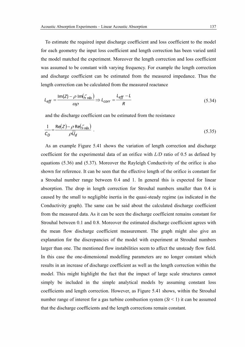
Acoustic Absorption Experiments – Linear Acoustic Absorption 137
To estimate the required input discharge coefficient and loss coefficient to the model
for each geometry the input loss coefficient and length correction has been varied until
the model matched the experiment. Moreover the length correction and loss coefficient
was assumed to be constant with varying frequency. For example the length correction
and discharge coefficient can be estimated from the measured impedance. Thus the
length correction can be calculated from the measured reactance
( )R
LLL
ZL eff
correff−
=⇒−
=Rρ
ζρ visIm)Im( ( 5.34)
and the discharge coefficient can be estimated from the resistance
( ) ( )dD U
ZC ρ
ζρ visReRe −=
1 . ( 5.35)
As an example Figure 5.41 shows the variation of length correction and discharge
coefficient for the experimental data of an orifice with L/D ratio of 0.5 as defined by
equations ( 5.36) and ( 5.37). Moreover the Rayleigh Conductivity of the orifice is also
shown for reference. It can be seen that the effective length of the orifice is constant for
a Strouhal number range between 0.4 and 1. In general this is expected for linear
absorption. The drop in length correction for Strouhal numbers smaller than 0.4 is
caused by the small to negligible inertia in the quasi-steady regime (as indicated in the
Conductivity graph). The same can be said about the calculated discharge coefficient
from the measured data. As it can be seen the discharge coefficient remains constant for
Strouhal between 0.1 and 0.8. Moreover the estimated discharge coefficient agrees with
the mean flow discharge coefficient measurement. The graph might also give an
explanation for the discrepancies of the model with experiment at Strouhal numbers
larger than one. The mentioned flow instabilities seem to affect the unsteady flow field.
In this case the one-dimensional modelling parameters are no longer constant which
results in an increase of discharge coefficient as well as the length correction within the
model. This might highlight the fact that the impact of large scale structures cannot
simply be included in the simple analytical models by assuming constant loss
coefficients and length correction. However, as Figure 5.41 shows, within the Strouhal
number range of interest for a gas turbine combustion system (St < 1) it can be assumed
that the discharge coefficients and the length corrections remain constant.

Acoustic Absorption Experiments – Linear Acoustic Absorption 138
Table 5.1 summarises the discharge coefficients and length corrections which
produced the best fit to the experimental data. Moreover the measured mean flow
discharge coefficients are also shown for the used orifice plates. Initially for orifice
geometries with L/D smaller than two it can be seen that the mean flow discharge
coefficient is sufficient for a good match of the modelling data to the experimental data.
This is shown in the comparisons of the measured and predicted Rayleigh Conductivity
using discharge coefficient CD,2 and the length corrections in Table 5.1 for L/D = 0.25,
0.5 and 1.98 in Figure 5.42 to Figure 5.44. It can be seen that the model matches the
experimental data very well. Therefore this confirms that the mean flow discharge
coefficient can be used in the linear acoustic model for an accurate prediction of
aperture CD with small L/D.
L/D CD,1 from plenum fed steady flow measurement
CD,2 from best fit of acoustic model
Lcorr from best fit of acoustic model
0.14 0.62 0.62 0.33
0.25 0.63 0.63 0.61
0.5 0.73 0.73 0.26
0.76 0.79 0.81 0.13
1 0.83 0.83 0.62
1.5 0.81 0.81 0.71
1.98 0.81 0.81 1.06
2.4 0.81 0.81 1.1
3 0.8 0.81 1.35
5 0.8 ~0.81 1.8
6.8 0.77 ~0.81 2.46
10 0.75 ~0.81 3.1 Table 5.1 Measured length corrections and discharge coefficients, cylindrical aper-
tures
However, for L/D ratios larger than two the discrepancy between the measured mean
flow discharge coefficient CD,1 and the matched coefficient CD,2 values increases.
Moreover it seems as if larger discharge coefficients are required to match the model to

Acoustic Absorption Experiments – Linear Acoustic Absorption 139
the experimental result. Figure 5.45 shows an example for the measurement and
modelling result for L/D of 6.8 using CD,2 and the length correction form Table 5.1. It
seems as if an even larger discharge coefficient is needed to match the data more
accurately. As the aperture length increases to geometries with L/D larger than two the
mean flow field characteristic within the orifice changes. Thus the interaction of the
unsteady flow with the orifice internal boundary layer becomes more important. Hence
the influence of the viscosity model for larger L/D orifice geometries will be assessed in
the following section.
5.9.2 Sources of Errors in the Analytical Modelling for Apertures with Large Length-to-Diameter Ratios
The previous section highlighted that the analytical model showed larger
discrepancies for the prediction of the admittance for apertures with L/D ratios larger
than two. Moreover as Table 5.1 showed the input discharge coefficient to the model for
the long apertures was required to be larger than the measured discharge coefficient.
The reasons for the increasing errors and deviations from the mean flow discharge
coefficient could be caused by changes in the flow behaviour through the aperture. This
is illustrated in Figure 5.46 for a short aperture with L/D < 2 and a long aperture with
L/D > 2. It can be seen that for the case of a short aperture the inflow into the orifice
generates a vena contracta, with the minimum area Ad being at the point where the
stream lines passing through the aperture are parallel (see section 2.1). In this way the
discharge coefficient is a measure of the area contraction between the aperture AD and
the area of the vena contracta. The viscosity effect within the aperture is negligible due
to the short length of the orifice. In this case the mean flow discharge coefficient is
agreeing well with the discharge coefficient derived from the acoustic experiment as
discussed in section 5.9.1. Based on the comparisons between measurements and
modelling in these cases it seems sufficient to model the acoustic resistance with the
measured discharge coefficient and the model was successfully applied to orifice
geometries from L/D of 0.14 to 2 (e.g. Figure 5.42 to Figure 5.44). However for the case
of a long aperture (L/D > 2) the measured mean flow discharge coefficient is a measure
of the losses associated with the inflow into the aperture, the viscous losses inside the
orifice and its associated velocity profile as well as the loss generated by the outflow

Acoustic Absorption Experiments – Linear Acoustic Absorption 140
profile of the aperture. Hence an acoustic modelling method has to be able to reproduce
the complex processes with a representative loss coefficient and unsteady viscosity
model. In the current model the viscosity is explicitly modelled with an unsteady
viscosity expression shown in Bellucci et. al. (2004) which was based on Kirchhoff
(1868). A similar expression is also shown in Keller and Zauner (1995). The viscosity
term is only accounting for the loss due to the unsteady flow across the boundary layer.
Another model which is simulating unsteady laminar Poiseuille flow within the
apertures can be found for example by Bellucci et. al. (2004b) but has not been used in
this work. However the choice of the most representative friction model, in addition to
the accurate prediction of the inflow and outflow profiles and their unsteady behaviour
is thought important and most likely the reason for the observed discrepancies.
A brief investigation of the impact of the viscosity and loss coefficients is shown in
Figure 5.47 which compares the predicted energy loss by the model with the measured
acoustic loss from experiments described in section 3.2.1 and 5.3. Two variations of the
model have been applied to the calculation. A first prediction was conducted using CD,2
and the length correction from Table 5.1 as an input, also including the viscosity term in
the calculation. In this case the loss coefficient is thought to represent the inflow and
outflow losses of a reattaching orifice flow field (e.g. L/D = 2) without the influence of
the boundary layer viscosity, which is therefore modelled by the unsteady viscosity
model. The second option was to use the mean flow discharge coefficient CD,1 from
Table 5.1 without the viscosity terms. Thus the viscous losses due to the unsteady flow
are thought to be negligible and the viscous losses are included in the mean flow
discharge coefficient. Both options gave the same result as can be seen in Figure 5.47
indicating either method would be an option to model longer apertures. The proposed
methods to model long apertures will be further investigated in chapter 8.3.3 where the
damping characteristics of multi-aperture liners with large L/D ratios are assessed.
In general for the practical engineering applications considered in this work the model
captures the pulsatile flow behaviour well. However this model relies on input
parameters such as loss coefficients (based on CD), length corrections and adequate
viscosity models. As a first assumption in the linear acoustic regime with Strouhal
numbers smaller than one the loss coefficients and length corrections are assumed to be

Acoustic Absorption Experiments – Linear Acoustic Absorption 141
constant. In this case no unsteady flow structures such as large scale vortex rings are
present in the pulsatile flow field and the structures in the shear layer do not seem to
have a particular important role in the sense that they do not affect the jet flow in a
positive or negative manner. Unless the excitation frequencies are near self-excited jet
flow instabilities (as for L/D = 0.5 geometries Figure 5.38). In this case the model
deviates from the measurement. This suggests that flow field structures within the shear
layers have an effect upon the Conductivity of the orifice which cannot be represented
by the model unless the loss coefficients and the length correction allow for this
behaviour. In this case the assumptions for the loss coefficient are too simple to predict
shear layer instabilities. This would be the advantage of a vortex sheet model as
described in the previous section. For example Bellucci et. al. (2004b) have used the
described Rayleigh Conductivity by Howe (1979b) to predict the loss coefficient based
on the vortex sheet model. However the discrepancies shown in section 5.8 indicate that
this approach would need improvements. The data given by Jing and Sun (2000)
indicated that flow instabilities could be captured. Hence improved vortex sheet models
with detailed jet trajectories could be used to generate Strouhal number dependent loss
coefficients. Moreover advanced CFD techniques (e.g. Mendez and Eldredge (2009) or
Gunasekaran and McGuirk (2011)) could be applied to improve the accuracy of the used
loss coefficients and aperture internal viscosity models.
5.10 Closure In this chapter the fundamental acoustic characteristics relating to linear absorption
has been discussed. It was shown that changes in orifice geometry, in terms of gas
turbine combustion system representative L/D ratios, result in changes in the measured
admittance of the Rayleigh Conductivity. The changes in admittance are associated with
changes in the steady flow discharge coefficients as well as the increased mass inertia
due to the length of the aperture. In fact within the linear quasi-steady regime increases
in the orifice discharge coefficients lead to increases in admittance with the maximum
admittance being reached for ideal discharge coefficients of one provided by a
Bellmouth orifice shape. However, for a fixed geometric area the increasing mean mass
flow through the aperture, due to increasing discharge coefficient, means there is no
benefit in acoustic loss per unit mass flow. Thus within a combustion system orifice

Acoustic Absorption Experiments – Linear Acoustic Absorption 142
geometry the linear absorption is governed by a pulsatile flow field which subsequently
dissipates due to turbulence. The acoustic energy is therefore transformed into kinetic
energy of the unsteady jet flow; with the maximum energy transfer is limited to the
quasi-steady regime. Hence the maximum acoustic absorption for a given pressure
amplitude and mean mass flow consumption is achieved in the linear quasi-steady
regime independent of orifice geometry.
It was shown that the Rayleigh Conductivity model based on the theory described by
Howe (1979b) agrees with the measured Rayleigh Conductivity for an orifice of L/D of
0.5 up to a Strouhal number of 0.9. This model was derived on the assumption of a thin
cylindrical shear layer and infinitesimal thin apertures. Hence the model can only be
applied to small L/D orifices. Moreover some discrepancies are shown in the quasi-
steady (low Strouhal number) regime which showed that the model is only valid for thin
apertures with a discharge coefficient of 0.7. This discrepancy might be caused by the
assumption of a thin cylindrical shear layer compared to a vorticity profile surrounding
the unsteady jet.
The modified Howe model was able to predict the measured Conductivities for orifice
geometries with L/D values larger than 0.5. However the described increasing
admittance, with increasing mean flow discharge coefficient within the quasi-steady
regime, could not be reproduced by the modified Howe model. The modified Howe
model is a length corrected version of the Howe model and relies on the Rayleigh
Conductivity curve for an infinitesimal thin aperture with a thin cylindrical shear layer.
This Rayleigh Conductivity is only a function of Strouhal number and thus the mean
velocity of the vorticity within the thin shear layer. Hence assuming that this velocity
can be estimated by the mean flow discharge coefficient could cause erroneous results
within the length modified model.
A model based on a momentum balance by Bellucci et. al. (2004) is capable of
reproducing the measured behaviour in the low Strouhal number regime and is the
preferred option for practical engineering applications. This model agrees with the
quasi-steady theory in the low Strouhal number regime and agrees with the observed
changes in admittance with changing aperture L/D. However the model is only accurate
as long as the aperture unsteady loss coefficient and length correction parameters

Acoustic Absorption Experiments – Linear Acoustic Absorption 143
remain constant as a first approximation. This is valid as long as there are no large
vortex structures generated within the jet flow shear layer as, for example, in the
vicinity of natural jet flow instabilities. Nevertheless this approach seems sufficient for
gas turbine combustion system geometries investigated in this work as the Strouhal
number remains low and therefore far away from natural occurring flow instabilities
through the aperture. However for orifice plates with L/D larger than two the analytical
modelling becomes more challenging. In this case the mean flow discharge coefficients
are no longer a sole measure of area contraction, but are also affected by the viscous
drag due to the boundary layer within the aperture. Moreover the effect of the unsteady
viscosity models is increasing with aperture length. Thus the use of an adequate
viscosity model representative of the aperture internal flow field, together with a
meaningful inflow and outflow loss coefficient, becomes important.

Acoustic Absorption Experiments – Linear Acoustic Absorption 144
Figures
Incident acoustic wave amplitude |B-| in dB^
0.0
0.1
0.2
0.3
0.4
0.5
0.6
110 115 120 125 130 135 140 145 150
Abs
orpt
ion
coef
ficie
nt ∆
dp/p = 2.9%
dp/p = 2%
dp/p = 1%
dp/p = 0.5%
Figure 5.1: Linear acoustic absorption with mean flow, plate number 1, L/D = 0.47,
f = 125Hz
0.0
0.1
0.2
0.3
0.4
0.5
0.6
115 120 125 130 135 140 145 150
Abso
rptio
n co
effic
ient
∆
dp/p = 0.8%
dp/p = 0.5%
dp/p =0.3%
dp/p = 0.1%
Incident acoustic wave amplitude |B-| in dB^
Figure 5.2: Linear acoustic absorption with mean flow plate number 3, L/D = 0.5, f = 62.5 Hz

Acoustic Absorption Experiments – Linear Acoustic Absorption 145
0
0.1
0.2
0.3
0.4
0.5
0.6
0 1 2 3 4 5 6 7 8
Adm
ittan
ce -
δ
Strouhal number - St
Howe (1979b)Measurememt L/D 0.47 - D = 12.7 mmMeasurement L/D = 0.5 - D = 9.1 mm
Figure 5.3: Measured admittance and comparison to theory from Howe (1979b),
Plate numbers 1 and 3.
0.00
0.02
0.04
0.06
0.08
0.10
0.12
0.14
110 115 120 125 130 135 140 145 150
Adm
ittan
ce -
δ
Plate 2, St = 0.022, Re = 7281
Plate 2, St = 0.022, Re = 14574
Plate 4, St = 0.059, Re = 20260
Plate 4, St = 0.059, Re = 40473
Figure 5.4: Measured admittance at constant Strouhal number and varying Reyn-
olds number for Plate numbers 2 and 4.

Acoustic Absorption Experiments – Linear Acoustic Absorption 146
0.00
0.05
0.10
0.15
0.20
0.25
0.30
136 138 140 142 144 146 148
Abso
rptio
n co
effic
ient
∆L/D 0.5
L/D 2.4
Incident acoustic wave amplitude |B-| in dB^
Figure 5.5: Comparison of absorption coefficient. Plate number 3, L/D = 0.5 and
plate number 7, L/D = 2.4. f = 62.5Hz, dp/p = 0.8%.
0.00
0.05
0.10
0.15
0.20
0.25
0.30
0.35
0 1 2 3 4 5 6 7 8
Abso
rptio
n co
effic
ient
∆
L/D
dp/p = 1%dp/p = 0.8%dp/p = 0.5%dp/p = 0.3%dp/p = 0.1%
Figure 5.6: Absorption coefficients for various L/D ratios at a range of pressure
drops. Plate numbers 3 to 11.

Acoustic Absorption Experiments – Linear Acoustic Absorption 147
0.5
0.6
0.7
0.8
0.9
1.0
0 1 2 3 4 5 6 7 8 9 10 11
Dis
char
ge C
oeffi
cein
t CD
L/D
Lichtarowicz et. al. (1965)
Measured
Figure 5.7: Discharge Coefficient measurement for various L/D ratios. Plate num-
bers 3 to 11
0.10
0.12
0.14
0.16
0.18
0.20
0.22
0.24
0.5 0.6 0.7 0.8 0.9 1 1.1 1.2 1.3 1.4
Abso
rptio
n co
effic
ient
-∆
Discharge Coefficient - CD
Cylindrical
Conical 30 degrees
Conical 45 degrees reverse
Conical 45 degrees
Conical 60 degrees
Sharp edged, 45 degrees
Stepped
Bellmouth
Figure 5.8: Absorption coefficients for various orifice shapes at a pressure drop of
dp/p = 0.5%.

Acoustic Absorption Experiments – Linear Acoustic Absorption 148
Standard mean flow direction
Flow direction
Reverse mean flow direction
Flow direction
Figure 5.9: Definition of flow direction through shaped orifice
0.0
0.5
1.0
1.5
2.0
2.5
3.0
3.5
4.0
4.5
5.0
0 200 400 600 800 1000 1200
Rea
ctan
ce -
X Z/ρ
c
Frequency in Hz
theory
Experiment L/D = 0.5
Figure 5.10: Orifice reactance measurement and comparison to theoretical values.
Plate number 20, L/D = 0.5.

Acoustic Absorption Experiments – Linear Acoustic Absorption 149
-40
-30
-20
-10
0
10
20
30
40
50
60
0 200 400 600 800 1000 1200
Res
ista
nce
-Re(
Z)
Frequency in Hz
Measured resistance
Radiation resistance theory
Figure 5.11: Comparison of measured resistance and theoretical radiation re-
sistance. Plate number 20, L/D = 0.5.
-0.2
0.0
0.2
0.4
0.6
0.8
1.0
1.2
0 0.2 0.4 0.6 0.8 1 1.2 1.4 1.6 1.8 2
Con
duct
ivity
/2R
Strouhal number - St
AdmittanceInertia
Figure 5.12: Measured Rayleigh Conductivity. Plate number 20, L/D = 0.5.

Acoustic Absorption Experiments – Linear Acoustic Absorption 150
-0.2
0.0
0.2
0.4
0.6
0.8
1.0
1.2
0 0.2 0.4 0.6 0.8 1 1.2 1.4 1.6 1.8 2 2.2 2.4 2.6 2.8 3
Con
duct
ivity
/2R
Strouhal number - St
Admittance
Inertia
Howe admittance
Howe Inertia
Figure 5.13: Measured Rayleigh Conductivity and comparison to Howe (1979b).
Plate number 20, L/D = 0.5.
0.0
0.2
0.4
0.6
0.8
1.0
0 0.2 0.4 0.6 0.8 1 1.2 1.4 1.6 1.8 2
Adm
ittan
ce -
δ
Strouhal number - St
L/D = 0.14
L/D = 0.25
L/D = 0.5
L/D = 0.76
L/D = 1
Figure 5.14: Measured admittance for plate numbers 18-22: 0.14 < L/D < 1.

Acoustic Absorption Experiments – Linear Acoustic Absorption 151
0.0
0.2
0.4
0.6
0.8
1.0
0 0.2 0.4 0.6 0.8 1 1.2 1.4 1.6 1.8 2
Iner
tia -
Γ
Strouhal number - St
L/D = 0.14L/D = 0.25L/D = 0.5L/D = 0.76L/D = 1
Figure 5.15: Measured inertia for plate numbers 18-22: 0.14 < L/D < 1.
_
Figure 5.16: Orifice reactance for plate numbers 18-22, 24, 27 and 29.

Acoustic Absorption Experiments – Linear Acoustic Absorption 152
0
1
2
3
4
5
0 0.2 0.4 0.6 0.8 1 1.2 1.4 1.6 1.8 2
Impe
danc
e -Z
/ρU
D
Strouhal number - St
L/D = 0.25 - Resistance
L/D = 1 - Resistance
L/D = 0.25 - Reactance
L/D = 1 - Reactance_
L/D = 1resistiveregime
L/D = 1reactiveregime
L/D = 0.25resistiveregime
Figure 5.17: Orifice impedance for plate numbers 19 and 22: L/D of 0.25 and 1.
0.0
0.1
0.2
0.3
0.4
0.5
0.6
0 0.1 0.2 0.3 0.4 0.5
Adm
ittan
ce -
δ
Strouhal number - St
L/D = 0.5
L/D = 1.98
L/D = 5
L/D = 10
Figure 5.18: Measured admittance for plate number: 20, 24, 27 and 29.
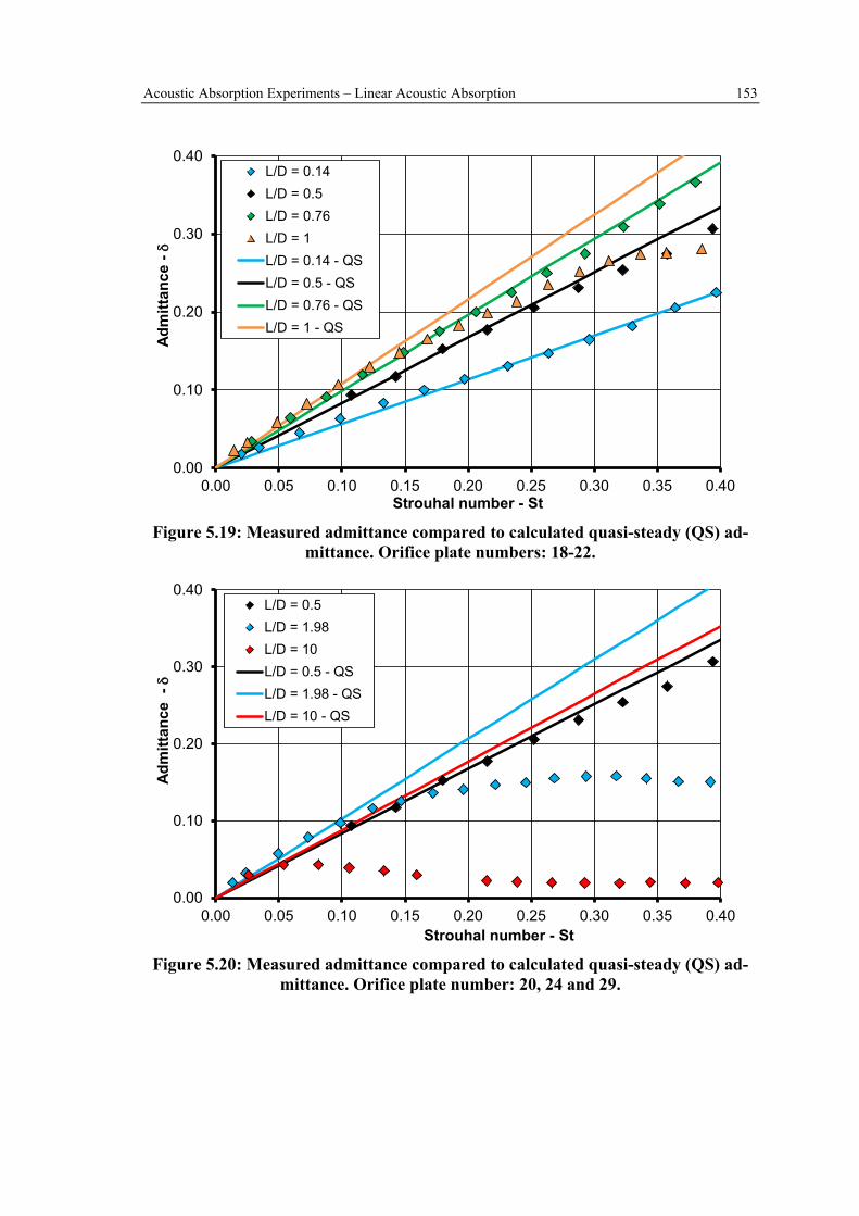
Acoustic Absorption Experiments – Linear Acoustic Absorption 153
0.00
0.10
0.20
0.30
0.40
0.00 0.05 0.10 0.15 0.20 0.25 0.30 0.35 0.40
Adm
ittan
ce -
δ
Strouhal number - St
L/D = 0.14L/D = 0.5L/D = 0.76L/D = 1L/D = 0.14 - QSL/D = 0.5 - QSL/D = 0.76 - QSL/D = 1 - QS
Figure 5.19: Measured admittance compared to calculated quasi-steady (QS) ad-
mittance. Orifice plate numbers: 18-22.
0.00
0.10
0.20
0.30
0.40
0.00 0.05 0.10 0.15 0.20 0.25 0.30 0.35 0.40
Adm
ittan
ce -
δ
Strouhal number - St
L/D = 0.5L/D = 1.98L/D = 10L/D = 0.5 - QSL/D = 1.98 - QSL/D = 10 - QS
Figure 5.20: Measured admittance compared to calculated quasi-steady (QS) ad-
mittance. Orifice plate number: 20, 24 and 29.

Acoustic Absorption Experiments – Linear Acoustic Absorption 154
0.00
0.10
0.20
0.30
0 0.025 0.05 0.075 0.1 0.125 0.15 0.175 0.2
Adm
ittan
ce -
δ
Strouhal number - St
L/D = 1.98
L/D = 3
L/D = 5
L/D = 6.8
L/D = 1.98 - QS
L/D = 6.8 - QS
Figure 5.21: Measured admittance compared to calculated quasi-steady (QS) flow
resistance. Effusion cooling geometries, orifice plate number: 24, 26-28.
0.0
0.2
0.4
0.6
0.8
1.0
1.2
1.4
1.6
0 0.2 0.4 0.6 0.8 1 1.2 1.4 1.6
Adm
ittan
ce -
δ
Strouhal number - St
L/D = 0.5
L/D = 0.5 - Bellmouth
L/D = 0.5 QS
L/D = 0.5 QS - Bellmouth
Figure 5.22: Admittance of Bellmouth orifice geometry compared to cylindrical
orifice. Plate number 20 and 31.
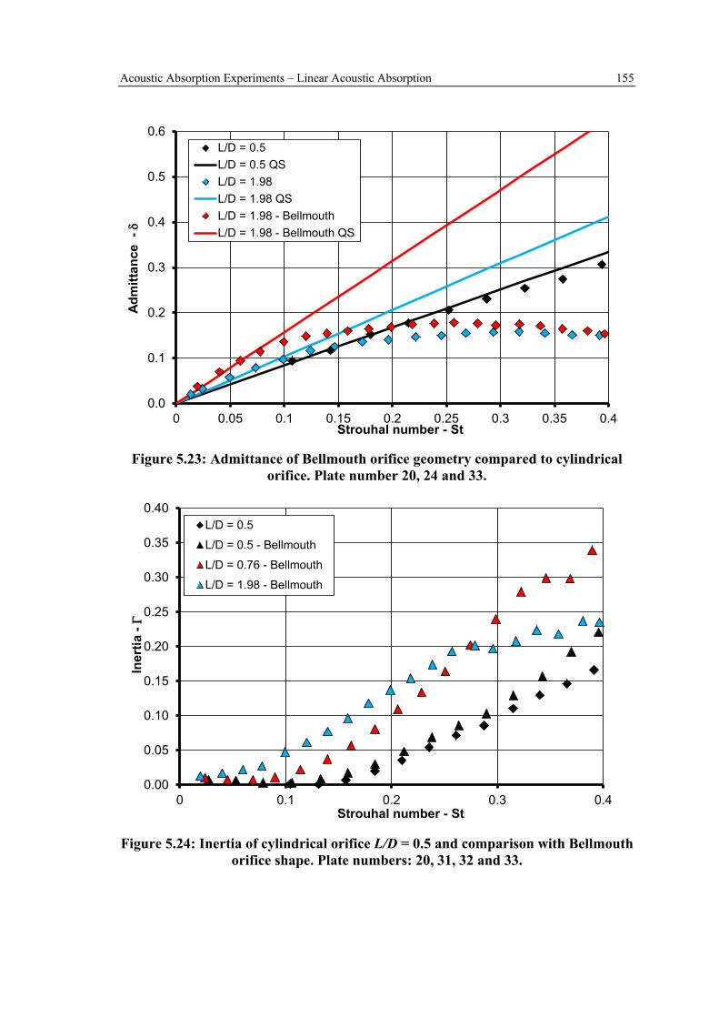
Acoustic Absorption Experiments – Linear Acoustic Absorption 155
0.0
0.1
0.2
0.3
0.4
0.5
0.6
0 0.05 0.1 0.15 0.2 0.25 0.3 0.35 0.4
Adm
ittan
ce -
δ
Strouhal number - St
L/D = 0.5L/D = 0.5 QSL/D = 1.98L/D = 1.98 QSL/D = 1.98 - BellmouthL/D = 1.98 - Bellmouth QS
Figure 5.23: Admittance of Bellmouth orifice geometry compared to cylindrical
orifice. Plate number 20, 24 and 33.
0.00
0.05
0.10
0.15
0.20
0.25
0.30
0.35
0.40
0 0.1 0.2 0.3 0.4
Iner
tia -
Γ
Strouhal number - St
L/D = 0.5
L/D = 0.5 - Bellmouth
L/D = 0.76 - Bellmouth
L/D = 1.98 - Bellmouth
Figure 5.24: Inertia of cylindrical orifice L/D = 0.5 and comparison with Bellmouth
orifice shape. Plate numbers: 20, 31, 32 and 33.

Acoustic Absorption Experiments – Linear Acoustic Absorption 156
0.0
0.5
1.0
1.5
2.0
2.5
3.0
3.5
4.0
4.5
0 0.2 0.4 0.6 0.8 1 1.2 1.4 1.6
Πno
rm
Strouhal number - Std
L/D = 0.5L/D = 0.5 - BellmouthL/D = 0.76 - BellmouthL/D = 1.98 - Bellmouth
Figure 5.25: Normalised acoustic loss per unit mass flow, cylindrical orifice com-
parison with Bellmouth orifice shape. Plate numbers: 20, 31, 32 and 33.
0.0
0.5
1.0
1.5
2.0
2.5
3.0
3.5
4.0
4.5
5.0
0 0.2 0.4 0.6 0.8 1 1.2 1.4 1.6
Πno
rm
Strouhal number - Std
L/D = 0.14L/D = 0.25L/D = 0.5L/D = 0.76L/D = 1L/D = 1.98Ideal QS loss
x10-4
Figure 5.26: Normalised acoustic energy loss per unit mass flow. Plate numbers:
18-22 and 24, 0.14 < L/D < 1.98.

Acoustic Absorption Experiments – Linear Acoustic Absorption 157
-0.2
-0.1
0
0.1
0.2
0.3
0.4
0.5
0.6
0.7
0.8
0 0.2 0.4 0.6 0.8 1 1.2 1.4 1.6 1.8 2
Adm
ittan
ce -
δ
Strouhal number -St
ExperimentHowe modelModified Howe model
Figure 5.27: Comparison between measured and predicted admittance using Ray-
leigh Conductivity models. Plate number 20, L/D = 0.5
0
0.2
0.4
0.6
0.8
1
1.2
0 0.2 0.4 0.6 0.8 1 1.2 1.4 1.6 1.8 2
Iner
tia -
Γ
Strouhal number -St
ExperimentHowe modelModified Howe model
Figure 5.28: Comparison between measured and predicted inertia using Rayleigh
Conductivity models. Plate number 20, L/D = 0.5.

Acoustic Absorption Experiments – Linear Acoustic Absorption 158
0
0.1
0.2
0.3
0.4
0.5
0.6
0.7
0.8
0 0.2 0.4 0.6 0.8 1 1.2 1.4 1.6 1.8 2 2.2
Adm
ittan
ce -
δ
Strouhal number -St
Experiment
Howe model
Modified Howe model
Figure 5.29: Comparison between measured and predicted admittance using Ray-
leigh Conductivity models. Plate number 19, L/D = 0.25.
0
0.1
0.2
0.3
0.4
0.5
0.6
0.7
0.8
0.9
0 0.2 0.4 0.6 0.8 1 1.2 1.4 1.6 1.8 2 2.2
Iner
tia -
Γ
Strouhal number -St
Experiment
Howe model
Modified Howe model
Figure 5.30: Comparison between measured and predicted inertia using Rayleigh
Conductivity models. Plate number 19, L/D = 0.25.

Acoustic Absorption Experiments – Linear Acoustic Absorption 159
0.00
0.10
0.20
0.30
0.40
0 0.2 0.4 0.6 0.8 1
Adm
ittan
ce -
δ
Strouhal number -St
Experiment
Howe model
Modified Howe model
Figure 5.31: Comparison between measured and predicted admittance using Ray-
leigh Conductivity models. Plate number 24, L/D = 1.98.
0
0.1
0.2
0.3
0.4
0.5
0.6
0 0.2 0.4 0.6 0.8 1
Iner
tia -
Γ
Strouhal number -St
ExperimentHowe modelModified Howe model
Figure 5.32: Comparison between measured and predicted inertia using Rayleigh
Conductivity models. Plate number 24, L/D = 1.98.

Acoustic Absorption Experiments – Linear Acoustic Absorption 160
0.00
0.05
0.10
0.15
0.20
0 0.2 0.4 0.6 0.8 1
Adm
ittan
ce -
δ
Strouhal number -St
Experiment
Howe model
Modified Howe model
Figure 5.33: Comparison between measured and predicted admittance using Ray-
leigh Conductivity models. Plate number 28, L/D = 6.8.
0.00
0.05
0.10
0.15
0.20
0 0.2 0.4 0.6 0.8 1
Iner
tia -
Γ
Strouhal number -St
ExperimentHowe modelModified Howe model
Figure 5.34: Comparison between measured and predicted inertia using Rayleigh
Conductivity models. Plate number 28, L/D = 6.8.

Acoustic Absorption Experiments – Linear Acoustic Absorption 161
dp/p = 1%
0.0
2.0
4.0
6.0
8.0
10.0
12.0
0 1 2 3 4 5 6 7 8 9 10
ΠP
L/D
Experiment
Howe model
Modified Howe model
x10-7
dp/p = 0.8%
0.0
2.0
4.0
6.0
8.0
10.0
12.0
0 1 2 3 4 5 6 7 8 9 10
ΠP
L/D
x10-7
dp/p = 0.5%
0.0
2.0
4.0
6.0
8.0
10.0
12.0
0 1 2 3 4 5 6 7 8 9 10
ΠP
L/D
x10-7
dp/p = 0.3%
0.0
2.0
4.0
6.0
8.0
10.0
12.0
0 1 2 3 4 5 6 7 8 9 10
ΠP
L/D
x10-7
Figure 5.35: Comparison between experiments and Rayleigh Conductivity models
from acoustic absorption coefficient measurements. Plate numbers: 3 – 11.

Acoustic Absorption Experiments – Linear Acoustic Absorption 162
0.0
2.0
4.0
6.0
8.0
10.0
12.0
0 1 2 3 4 5 6 7 8 9 10
ΠP
L/D
Experiment
Measured discharge coefficient
x10-7
CD = 0.5
Figure 5.36: Effect of discharge coefficient on the comparison between experiments
and the modified Howe model. Plate numbers: 3 – 11, dp/p = 0.5%.

Acoustic Absorption Experiments – Linear Acoustic Absorption 163
dp/p = 1%
0.0
2.0
4.0
6.0
8.0
10.0
12.0
0 1 2 3 4 5 6 7 8 9 10
ΠP
L/D
ExperimentQuasi-steady model
x10-7
dp/p = 0.8%
0.0
2.0
4.0
6.0
8.0
10.0
12.0
0 1 2 3 4 5 6 7 8 9 10
ΠP
L/D
x10-7x10⁻⁷
dp/p = 0.5%
0.0
2.0
4.0
6.0
8.0
10.0
12.0
0 1 2 3 4 5 6 7 8 9 10
ΠP
L/D
x10-7
dp/p = 0.3%
0.0
2.0
4.0
6.0
8.0
10.0
12.0
0 1 2 3 4 5 6 7 8 9 10
ΠP
L/D
x10-7
Figure 5.37: Comparison between experiments and quasi-steady admittance model
for absorption coefficient experiments. . Plate numbers: 3 – 11.

Acoustic Absorption Experiments – Linear Acoustic Absorption 164
0
0.2
0.4
0.6
0.8
1
1.2
1.4
1.6
1.8
0 0.3 0.6 0.9 1.2 1.5
Con
duct
ivity
/2R
Strouhal Number - St
Measured inertia
Measured admittance
Bellucci et. al. inertia
Bellucci et. al. admittance
QS admittance
Figure 5.38: Predicted and measured Rayleigh Conductivity using theory based on
Bellucci et. al. Plate number 20, L/D = 0.5
0
0.1
0.2
0.3
0.4
0.5
0.6
0.7
0.8
0.9
1
0 0.3 0.6 0.9 1.2 1.5 1.8 2.1
Con
duct
ivity
/2R
Strouhal Number - St
Measured inertia
Measured admittance
Bellucci et. al. inertia
Bellucci et. al. admittance
QS admittance
Figure 5.39: Predicted and measured Rayleigh Conductivity using theory based on
Bellucci et. al. Plate number 19, L/D = 0.25.

Acoustic Absorption Experiments – Linear Acoustic Absorption 165
0.00
0.05
0.10
0.15
0.20
0.25
0.30
0.35
0.40
0 0.3 0.6 0.9 1.2 1.5
Con
duct
ivity
/2R
Strouhal Number - St
Measured inertia
Measured admittance
Bellucci et. al. inertia
Bellucci et. al. admittance
QS admittance
Figure 5.40: Predicted and measured Rayleigh Conductivity using theory based on
Bellucci et. al. Plate number 24, L/D = 1.98
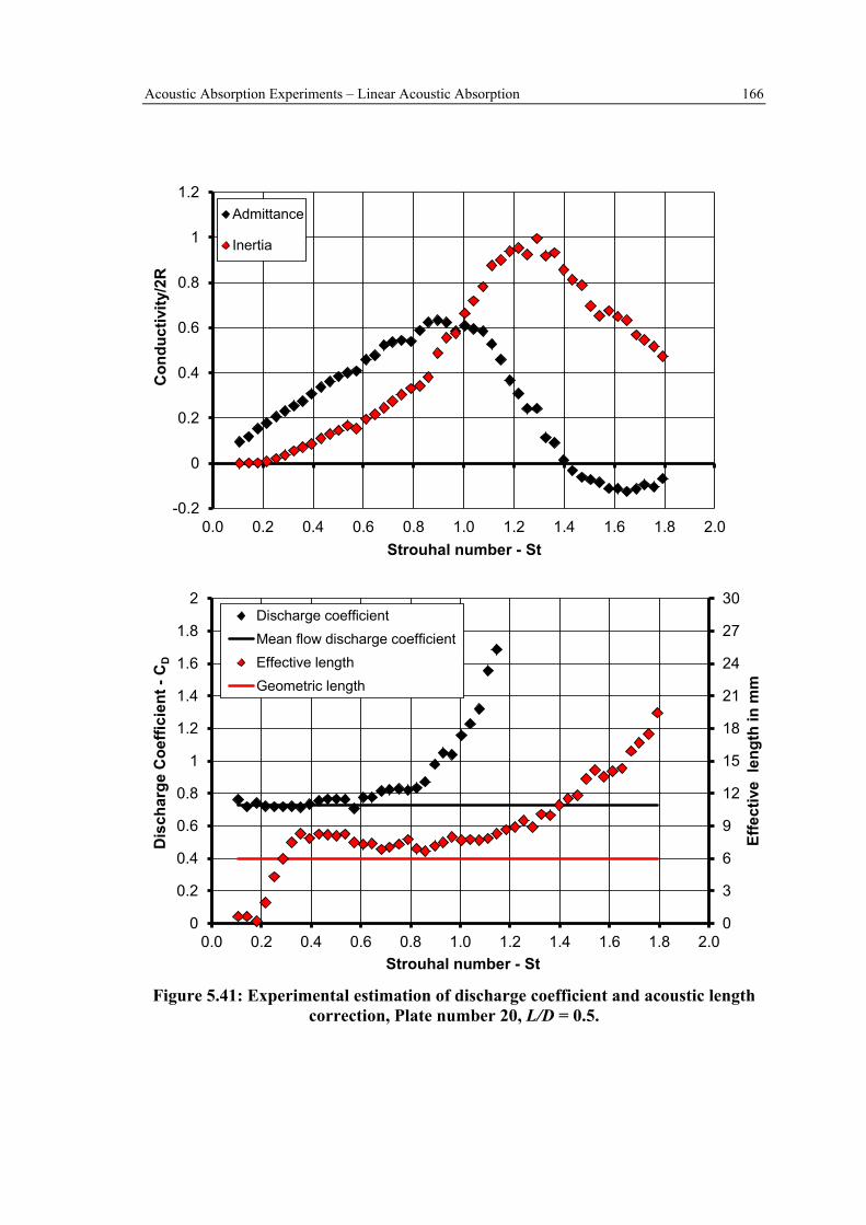
Acoustic Absorption Experiments – Linear Acoustic Absorption 166
-0.2
0
0.2
0.4
0.6
0.8
1
1.2
0.0 0.2 0.4 0.6 0.8 1.0 1.2 1.4 1.6 1.8 2.0
Con
duct
ivity
/2R
Strouhal number - St
Admittance
Inertia
0
3
6
9
12
15
18
21
24
27
30
0
0.2
0.4
0.6
0.8
1
1.2
1.4
1.6
1.8
2
0.0 0.2 0.4 0.6 0.8 1.0 1.2 1.4 1.6 1.8 2.0
Effe
ctiv
e le
ngth
in m
m
Dis
char
ge C
oeffi
cien
t -C
D
Strouhal number - St
Discharge coefficientMean flow discharge coefficientEffective lengthGeometric length
Figure 5.41: Experimental estimation of discharge coefficient and acoustic length
correction, Plate number 20, L/D = 0.5.
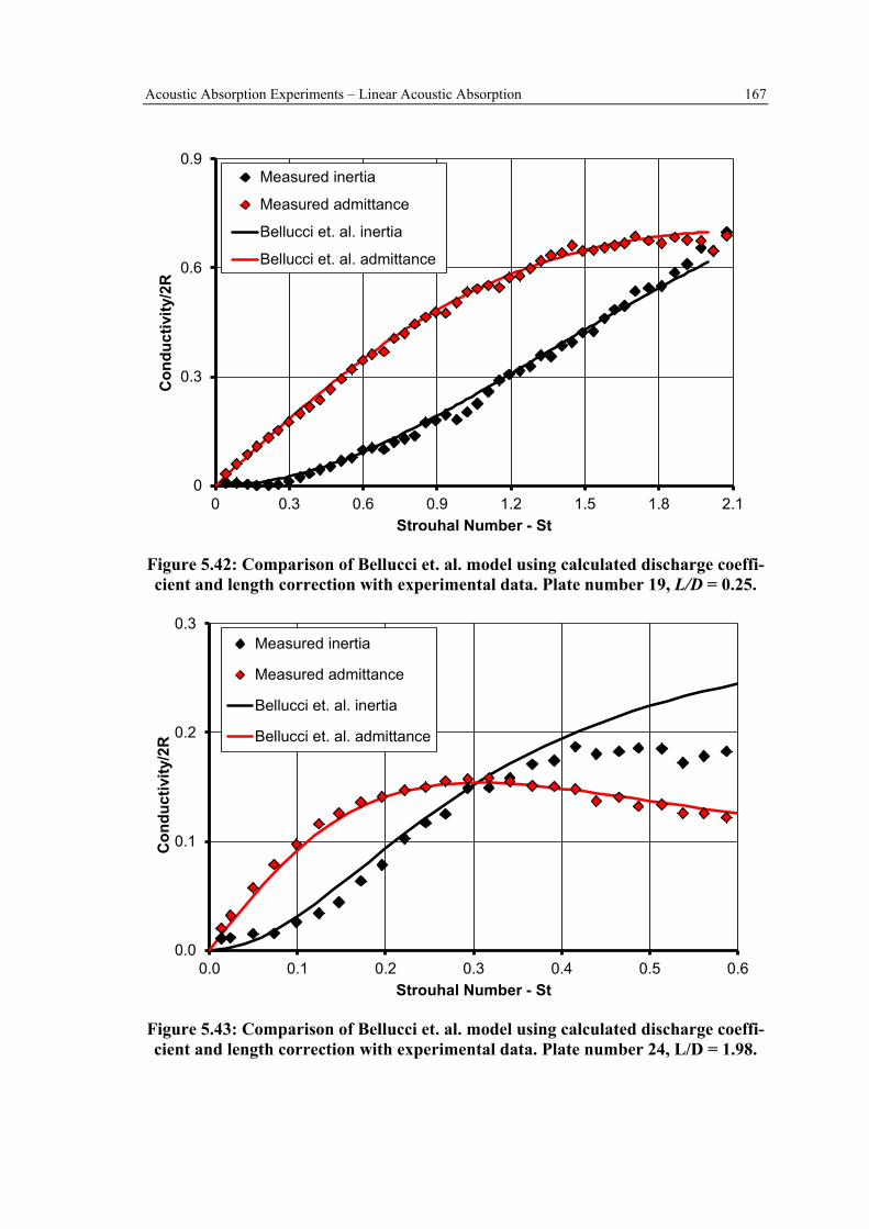
Acoustic Absorption Experiments – Linear Acoustic Absorption 167
0
0.3
0.6
0.9
0 0.3 0.6 0.9 1.2 1.5 1.8 2.1
Con
duct
ivity
/2R
Strouhal Number - St
Measured inertia
Measured admittance
Bellucci et. al. inertia
Bellucci et. al. admittance
Figure 5.42: Comparison of Bellucci et. al. model using calculated discharge coeffi-cient and length correction with experimental data. Plate number 19, L/D = 0.25.
0.0
0.1
0.2
0.3
0.0 0.1 0.2 0.3 0.4 0.5 0.6
Con
duct
ivity
/2R
Strouhal Number - St
Measured inertia
Measured admittance
Bellucci et. al. inertia
Bellucci et. al. admittance
Figure 5.43: Comparison of Bellucci et. al. model using calculated discharge coeffi-cient and length correction with experimental data. Plate number 24, L/D = 1.98.
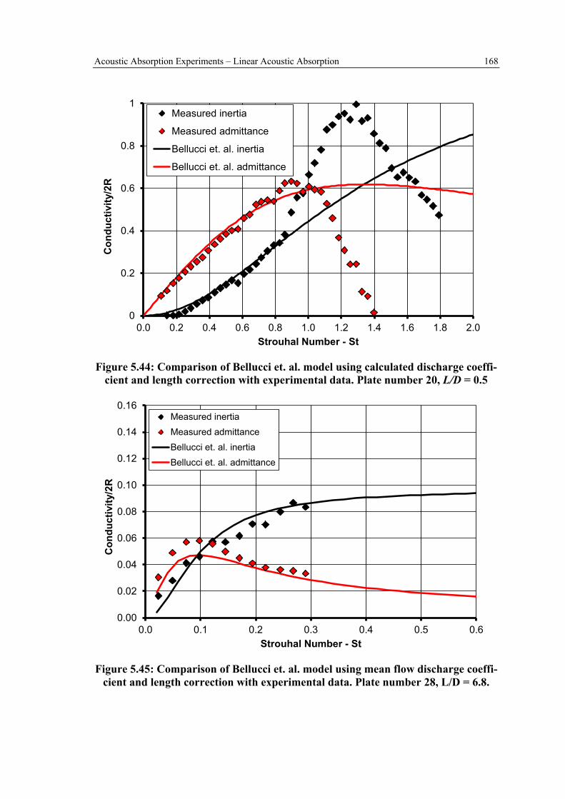
Acoustic Absorption Experiments – Linear Acoustic Absorption 168
0
0.2
0.4
0.6
0.8
1
0.0 0.2 0.4 0.6 0.8 1.0 1.2 1.4 1.6 1.8 2.0
Con
duct
ivity
/2R
Strouhal Number - St
Measured inertia
Measured admittance
Bellucci et. al. inertia
Bellucci et. al. admittance
Figure 5.44: Comparison of Bellucci et. al. model using calculated discharge coeffi-
cient and length correction with experimental data. Plate number 20, L/D = 0.5
0.00
0.02
0.04
0.06
0.08
0.10
0.12
0.14
0.16
0.0 0.1 0.2 0.3 0.4 0.5 0.6
Con
duct
ivity
/2R
Strouhal Number - St
Measured inertiaMeasured admittanceBellucci et. al. inertiaBellucci et. al. admittance
Figure 5.45: Comparison of Bellucci et. al. model using mean flow discharge coeffi-
cient and length correction with experimental data. Plate number 28, L/D = 6.8.

Acoustic Absorption Experiments – Linear Acoustic Absorption 169
ADAd
Short orifice with L/D < 2
Long orifice with L/D > 2
Figure 5.46: Short and long orifice mean flow profiles, underlying pictures from Hay and Spencer (1992)
0.0
2.0
4.0
6.0
8.0
10.0
12.0
14.0
0 1 2 3 4 5 6 7 8 9 10
ΠP
L/D
Experiment
Bellucci model with viscosity
Bellucci model without viscosity
x10-7
CD,2
CD,1
Figure 5.47: Comparison of Bellucci et. al. model using discharge coefficient and length correction from Table 5.1 with experimental absorption data, dp/p = 0.5%
Plate numbers 3-11.
Acoustic Absorption Results – Non-Linear Acoustic Absorption 170
6 Acoustic Absorption Results – Non-Linear Acoustic Absorption
Experiments to investigate the non-linear absorption characteristic of a generic orifice
were initially conducted without mean flow. The non-linear acoustic absorption is likely
to be observed if the unsteady velocity oscillation amplitude is of the order, or larger
than, the mean flow velocity. At these conditions the amount of absorption is dependent
on the excitation amplitude. Note the acoustic pressure amplitudes remained within the
linear acoustic regime (i.e. pp <<ˆ ) throughout the non-linear absorption experiments.
6.1 Optimum Non-Linear Acoustic Absorption The experiments without mean flow have been conducted on the absorption
coefficient test facility described in section 3.2.1. Figure 6.1 shows some example data
from an acoustic absorption measurement for a test case without mean flow (orifice
plate number 1). The absorption coefficient is shown with respect to the magnitude of
the complex pressure amplitude travelling from the loudspeakers towards the orifice.
The results, as also shown and described in Rupp et. al. (2010), indicate that the
absorption coefficient is a function of the incident acoustic energy (and hence
absorption is non-linear). It can be seen that the absorption coefficient increases
between 117dB and 135dB where the absorption coefficient reaches a value of 0.49.
However, further increases in the incident energy results in a decrease in absorption. It
could be argued that in excess of 135 dB the absolute amount of energy that can be
absorbed by the flow field is constant, and so the absorption coefficient decreases due to
the increasing incident energy. To investigate this behaviour further the acoustic energy
loss is compared to the incident acoustic energy flux in Figure 6.2. The acoustic energy
loss was estimated from the difference of incidental and reflected acoustic energy flux
in the duct (equation (5.3)). At excitation amplitudes higher than 135 dB the acoustic
energy absorbed still increases but at a rate which is less than the incident acoustic
energy flux. It is the decreasing rate at which the energy is lost with increasing pressure

Acoustic Absorption Results – Non-Linear Acoustic Absorption 171
amplitude that is responsible for the observed decrease in absorption coefficient at high
excitation levels (Figure 6.1).
This behaviour can be further expressed in terms of the measured impedance of the
orifice and comparing it to the normalised acoustic energy loss in Figure 6.3. In this
case the impedance is defined as the incident pressure amplitude onto the orifice divided
by the orifice velocity amplitude (i.e. DupZ ˆˆ= ). Moreover a theoretical reactance as
defined by Ingard and Ising (1967)
( ) ( )RLXZ Z 71.Im +== ρR ( 6.1)
is also included in Figure 6.3. It can be seen for small velocity amplitude (or incident
pressure amplitudes) the measured reactance agrees with the theoretical prediction
proposed by Ingard and Ising (1967). Furthermore it is shown that the reactance reduces
with increasing velocity amplitude. On the contrary the resistance of the aperture is
small at low pressure amplitudes and increases with increasing velocity amplitudes. In
general this characteristic is the same as shown in Ingard and Ising (1967). The acoustic
energy loss maximum occurs at a velocity amplitude of approximately 15 m/s. This
optimum is also located in the vicinity where the resistance and reactance are equal
(approximately at 12 m/s). Hence at velocity amplitudes below 12 m/s the aperture flow
field is reactive (dominated by the inertia forces due to the acceleration of the fluid in
the aperture) and for larger velocities (above 12 m/s) the flow field is dominated by the
resistance effects (viscous effects in any shear layer of the aperture flow field). The
resistance rapidly rises for larger velocity amplitudes whilst the reactance seems to
reduce to an asymptotic value. The acoustic absorption increases for velocity amplitudes
below 15 m/s. In this case the reactance reduces and thus the phase angle between
pressure and velocity amplitude reduces. However as the resistance becomes
significantly larger than the reactance the velocity amplitudes, relative to the incident
pressure amplitude, reduce. Therefore the acoustic loss relative to the acoustic pressure
amplitude decreases. This behaviour is confirmed in Figure 6.4 where the aperture
velocity amplitude is shown relative to the incident pressure amplitude. Initially, at low
amplitudes below 200 Pa, the velocity amplitude is increasing with a constant gradient
to approximately 15 m/s (p’ ~ u’). At this point the gradient changes and the velocity
amplitude increases at a lower rate than the increase in pressure amplitude (p’ ~ u’2).

Acoustic Absorption Results – Non-Linear Acoustic Absorption 172
When the orifice behaviour is described in terms of impedance it can be seen that
there are regions where (i) the reactance dominates, and (ii) the resistance dominates.
i) In reactance dominated regions the acoustic absorption increases with increasing
pressure amplitudes and is associated with a reduced effective length of the
orifice.
ii) In the resistance dominated region the acoustic absorption decreases with
increasing pressure amplitude and is associated with an orifice resistance. This
means the rate of increase in velocity amplitude relative to the incident pressure
amplitude is reduced.
6.2 Influence of Orifice Length upon Non-Linear Acoustic Absorp-tion
In a conventional combustion system various orifice geometries can be found with
hole length-to-diameter ratios ranging from L/D of 0.5 to 10. Figure 6.5 shows the non-
linear acoustic absorption characteristic for such orifice geometries. It can be seen that
the acoustic absorption increases with decreasing orifice length. Moreover the optimum
absorption occurs at smaller incident wave amplitudes as the L/D ratio decreases. If the
length of the orifice increases the inertial forces, due to the acceleration of a larger fluid
mass inside the orifice, must also increase and a reduction in velocity amplitude is
therefore expected. In terms of impedance this indicates an increased reactance
associated with the orifice flow field. This can be seen for the example of two orifice
plates with L/D of 0.5 and 1.98 in Figure 6.6. Note this data has been measured with
125 Hz forcing frequency. Nevertheless the basic principles explained with this data do
also apply for the data shown in Figure 6.5. As expected the measured impedance shows
an increased reactance for the longer aperture. Ultimately this leads to reduced velocity
amplitudes for the longer aperture as shown in Figure 6.7. Moreover the occurrence of
the optimum acoustic absorption coefficient appears at larger excitation pressure as the
cross-over point from the reactive regime to the resistive regime appears at higher
pressure amplitudes (Figure 6.6).
As already mentioned non-linear acoustic absorption is governed by vortex ring
structures shed from the rim of the orifice. With this in mind it is interesting to note the

Acoustic Absorption Results – Non-Linear Acoustic Absorption 173
observations of several authors whose investigations were not directly linked to that of
acoustic absorption as highlighted and discussed in Rupp et. al. (2010). For example
Gharib et. al. (1998), Linden and Turner (2001) or Jabbal et. al. (2006) have studied the
formation of vortex rings and the optimum conditions whereby the circulation in the
vortex core obtains a maximum value. It was not possible to increase the maximum
circulation of the vortex ring, and hence the kinetic energy associated with the vortex
ring, despite increasing the fluctuating velocity in the orifice used to form the rings.
Instead secondary flow features, e.g. wakes, start to absorb the energy and become
visible in the flow field. More details of the fluid dynamic properties of vortex rings can
be found in section 2.3. A formation number has been proposed which is a measure of
the velocity amplitude for a vortex ring which is based on the orifice diameter D and the
fluid slug length during half of the excitation cycle (see also equation 2.12):
( )
D
dttu
DL
T
D∫=
2
00
'
( 6.2)
Using the measured velocity amplitude in the aperture of the orifice and assuming a
sinusoidal time variation of this amplitude based on the fundamental forcing frequency
leads to the definition of the vortex ring formation number:
( )
'
ˆˆsinˆ
StRu
Du
D
dttu
DL DD
T
D12
2
00 ====∫
RR
R
.
( 6.3)
This approach is equivalent to assuming a top hat velocity profile issuing from the
aperture. To first order, the higher order harmonics can be ignored, as the amplitude of
the harmonic frequencies are greatly reduced compared to the fundamental mode
(Ingard (1970)). It can be seen that the formation number is inversely proportional to a
Strouhal number based on the unsteady velocity amplitude. Authors investigating
optimum vortex ring formation, e.g. Gharib et. al. (1998) or Jabbal et. al. (2006) state
L0/D = 4 or St’ = 0.25 for optimum vortex ring formation. The data presented in Figure
6.5 is now shown in Figure 6.8 relative to the vortex ring formation number L0/D. It can
be seen the optimum acoustic absorption does not coincide with one vortex ring

Acoustic Absorption Results – Non-Linear Acoustic Absorption 174
formation number. This becomes clearer in Figure 6.9 which shows the vortex ring
formation number at the maximum acoustic absorption. It can be seen that the location
of the optimum acoustic absorption does not collapse on the optimum vortex ring
formation number of four. The literature concerned with optimum vortex ring formation
(e.g. Gharib et. al. (1998), Aydemir et. al. (2012)) uses a pulsatile nozzle flow which is
characterised by a top hat velocity exit profile from the nozzle which generates the
vortex ring and unsteady jet flow. Moreover the influence of the flow field reactance
was not of interest for the mentioned experiments. The apparatus used in Jabbal et. al.
(2006), where a loudspeaker is exciting the flow field of an orifice with L/D = 1, is the
closest to the application in this work. Jabbal et. al. (2006) showed the optimum vortex
ring formation of L0/D of four which is close to the estimated formation number in this
work which shows a vortex ring formation number of five in Figure 6.9. The data
suggests that the formation number with changing L/D is showing two regimes as the
formation number at optimum acoustic absorption linearly varies with L/D. The slope of
the linear behaviour changes around an L/D ratio of one. This could be influenced by
the flow behaviour of the aperture. For example for short apertures the assumption of a
top hat velocity profile might not be valid. Hence this could change the slope of the
shown characteristic in Figure 6.9. As the flow reattaches within the longer L/D
apertures the generated exit profile could look more like a fully developed flow profile.
Furthermore the increased viscosity for long L/D ratios (larger than one) might also
effect the vortex ring formation. However, as already mentioned the optimum
absorption occurs in the region where the acoustic resistance and reactance are of equal
value. Due to the increased reactance for longer orifice plates (e.g. as shown in Figure
6.6) the occurrence of the optimum absorption occurs at larger velocity amplitudes and
therefore larger formation numbers. In the synthetic jet experiments of Gharib et. al.
(1998) or Jabbal et. al. (2006) it was important to maximise the amount of energy
transferred into the vortex core. For the purpose of the work in this thesis it is important
to maximise the kinetic energy flux of the aperture flow field at a given incident
pressure amplitude. The unsteady kinetic energy of the aperture flow field in the
acoustic measurements is described with the acoustic resistance and reactance where
both parameters in the non-linear absorption regime are a function of incident pressure
amplitude. Ultimately the changes in the described acoustic properties are caused by the

Acoustic Absorption Results – Non-Linear Acoustic Absorption 175
fluid dynamic properties of the vortex ring and the potential secondary flow structures.
Hence this is further investigated in the unsteady flow fields in chapter 7.
6.3 Comparison with Non-Linear Acoustic Absorption Models The model used to predict the non-linear acoustic absorption was developed by
Bellucci et. al. (2004). This model has been assessed in terms of its ability to predict the
experimental data. Moreover, the model was also used to derive the effective length and
the loss coefficients for the best match with the experimental data. The model is based
on a momentum balance across the orifice and has been introduced in detail in section
2.5.3. In this case the downstream pressure amplitude is set to zero as measured in the
experiment. Thus the momentum balance for the calculations shown in this section was
defined as:
012 =
+−+ DD
D
D
DusDvisDeff uu
uU
gC
puuli ˆˆˆ
ˆˆˆ ρρςRρ . ( 6.4)
Note the model is valid for the linear and non-linear acoustic absorption regime. This
characteristic of the model is controlled by the function ( )DD uUg ˆ in equation ( 6.4). If
the velocity amplitude is much smaller than the mean velocity the relationship between
incident pressure amplitude and velocity amplitude is linear. In the non-linear regime
the velocity amplitude is in the order of the mean velocity through the aperture or larger.
The experiments have been conducted in the absence of mean flow through the orifice.
Hence equation ( 6.4) with 0=DU reduces to
0341
2 =+−+ DDD
uDvisDeff uuC
puuli ˆˆˆˆˆπ
ρρςRρ , ( 6.5)
according to equation (2.55).
The non-linear equation ( 6.5) is solved using a non-linear numerical solver within
MATLAB. In this case the pressure amplitude was an input variable and the velocity
amplitude was the solution provided by the numerical solver. As the acoustic length of
the orifice and its discharge coefficient were not known a priori the length correction
and discharge coefficient were matched to reproduce the measured acoustic impedance.
Acoustic Absorption Results – Non-Linear Acoustic Absorption 176
Figure 6.10 shows a comparison of the measured impedance and the acoustic energy
loss without mean flow for two orifice plates: Plate number 19 with L/D = 0.25 and
Plate number 22 with L/D = 1. Note the acoustic loss is calculated from the measured
data as described in section 5.1 and normalised with the square of the incident pressure
amplitude. The non-linear model can be used to calculate the admittance of the aperture
which enables the loss calculation as described in equation (5.4) which leads to the
same result as in equation (2.62). Finally the calculated energy loss is also normalised
with the incident pressure amplitude. In general it can be seen, as also shown in the
previous section, that both the resistance and reactance are a function of excitation
pressure amplitude. However it seems as if the model agrees with the impedance of the
longer orifice (L/D = 1) much better than for the shorter orifice (L/D = 0.25). The
reactance of the longer orifice remains constant over a wider excitation amplitude (i.e.
up to L0/D of 2 instead of L0/D of 0.7 for the aperture with L/D = 0.25). Moreover the
resistance follows a linear trend to higher excitation amplitudes than for the shorter
orifice. The reason for the differences in measured reactance for the two apertures is
caused by the distribution of internal and external reactance. The aperture internal
reactance is governed by inertial forces accelerating the mass of the fluid within the
aperture. Whereas the external reactance of the aperture flow field is simulated with the
length correction. The external length correction is affected by the vortex ring
aerodynamic behaviour. For a thin aperture (L/D = 0.25) the external flow reactance
dominates. As the amplitudes increase so changes the unsteady flow field controlled by
the large scale structures and thus the aperture reactance is changing. For the long
aperture the internal reactance seems to have the larger influence upon the overall
reactance and hence the effect of the external flow field seems to have a reduced
influence upon the acoustic behaviour of the aperture.
The assumption of constant loss coefficient and length correction in the model is not
sufficient for the prediction of the impedance for the short orifice. Hence it cannot be
accurately reproduced which leads to discrepancies in the acoustic loss predictions. And
the model does only agree with the points where resistance and reactance are matched
with the experiment. The longer orifice however shows better agreement with modelled

Acoustic Absorption Results – Non-Linear Acoustic Absorption 177
impedance on the basis of constant loss coefficient and length correction and therefore
the acoustic loss is reproduced more accurately.
In general the modelling of the non-linear acoustic absorption behaviour is a
challenge with simple one dimensional calculation tools. The flow field in the non-
linear regime is complex due to large scale structures, such as vortex rings, which
influence the unsteady flow field. Moreover the nature of these structures is also
dependent on the excitation amplitude itself. This is simplified in a one dimensional
model by using acoustic length corrections and discharge coefficient. It is therefore not
surprising that the length correction or the loss coefficient is dependent on the excitation
amplitude. Furthermore this dependency needs to be estimated using empirical data as,
for example, conducted in Cummings (1986), Hersh et. al. (1999), Betts (2000) and
Bellucci et .al. (2004b). For the purpose of this work an investigation was conducted
into the flow field during non-linear absorption to understand the fluid dynamic nature
of the changes in length correction and loss coefficient. This will be discussed in the
following chapter.
6.4 Transition from Linear to Non-Linear Acoustic Absorption The transition from linear to non-linear absorption behaviour is of great importance
for the design of acoustic dampers within gas turbine combustion systems. Moreover it
is of importance in terms of the unsteady characteristic of the cooling flow through
effusion holes. In general acoustic damping devices connected to the combustion
chamber require a mean flow through the apertures for cooling purposes. If combustion
instabilities occur, at some point during the gas turbine operating envelope, and these
cannot be adequately controlled by the damping device the pressure amplitudes within
the combustion chamber rises. At this point transition from linear to non-linear
absorption can occur. Thus linear absorption models cannot predict the orifice velocity
amplitudes associated with the non-linear acoustic absorption and vice versa.
Investigating which parameters influence the transition and the point at which the
transition from linear to non-linear absorption occurs are important for several reasons.
The non-linear absorption characteristic will influence the limit cycle pressure
amplitude of the combustion instability. Thus accurate non-linear absorption models

Acoustic Absorption Results – Non-Linear Acoustic Absorption 178
will be necessary for thermo-acoustic pressure amplitude predictions. Moreover the
transition from linear to non-linear absorption changes the relationship between
unsteady velocity and acoustic pressure amplitude. With rising pressure amplitudes
relative to the mean aperture the risk of hot gas ingestion into the damper geometry or
cooling geometry increases. This will reduce the cooling effectiveness of the combustor
wall and, ultimately, could lead to overheating of the combustor wall. To be able to
predict the occurrence of hot gas ingestion is of great importance to understand the
velocity amplitude relative to the mean velocity through the apertures. Hence the
transition from linear to non-linear absorption needs to be understood and adequately
described.
6.4.1 Acoustic Absorption Coefficient Measurements during the Tran-sition from Linear to Non-linear Absorption
Figure 6.11 shows a summary of measured acoustic absorption coefficients for single
orifice geometries. In this case the absorption coefficient ∆ is shown with respect to the
incident wave amplitude. The figure shows an example of four orifice geometries with
length-to-diameter ratios of 0.5, 1.98, 3 and 6.8. For each of the geometries the
measured absorption coefficient at four test conditions is shown: dp/p of 0-0.5% mean
pressure drop resulting in a Strouhal number range from 0.08 to 0.19. In this case the
solid symbols represent the linear absorption regime (i.e. the acoustic absorption
coefficient is constant with pressure amplitudes) and the hollow symbols signify the
non-linear absorption regime (i.e. the acoustic absorption coefficient varies with
pressure amplitudes). For the geometry with L/D of 0.5 (Figure 6.11 a)) it can be seen
that for finite levels of pressure drop the non-linear absorption coefficients increase to a
maximum. This maximum value coincides with the non-linear absorption coefficient
without mean flow through the aperture. After reaching the maximum value, for the
cases with mean flow, all coefficients (with and without mean flow) converge onto the
same absorption coefficient for further increases in excitation pressure amplitude.
However this is not the same for all the shown examples. As Figure 6.11 b) shows the
absorption coefficient reduces in the non-linear acoustic absorption regime compared to
the linear acoustic absorption coefficient for dp/p = 0.1%. It can also be seen, e.g.
Figure 6.11 c) dp/p = 0.1%, that the linear absorption regime generates larger absorption

Acoustic Absorption Results – Non-Linear Acoustic Absorption 179
coefficients than the non-linear optimum absorption for the case with no mean flow. In
general all the data shows that the non-linear absorption behaviour with mean flow is
converging on the absorption coefficient characteristic of the non-linear regime without
mean flow. Hence the absorption coefficient increases or decreases during transition
from linear to non-linear absorption dependent on the level of the non-linear absorption
coefficient without mean flow. In other words, if the linear absorption is larger than the
non-linear absorption without mean flow the absorption coefficient reduces during
transition from the linear to the non-linear regime and vice versa. At high velocity
amplitude to mean velocity ratios the influence of the mean flow becomes insignificant.
Hence the convergence of the data with and without mean flow at large amplitudes in
the non-linear regime. In this case the flow field is governed by the same phenomena as
for the non-linear absorption regime without mean flow, i.e. pulsatile jet flows and the
presence of large scale vortex rings.
Figure 6.11 also shows that for the cases with mean flow the transition from linear to
non-linear absorption occurs at lower excitation amplitudes with reducing pressure
drops. Thus it is not the actual pressure amplitude which controls the point of transition,
it is the pressure amplitude relative to the mean pressure drop. Hence the transition can
occur at relative small pressure amplitudes if the mean pressure drop is sufficiently low.
As discussed in section 1.3.1.3 within the non-linear acoustic absorption regime the
pressure amplitude is proportional to the square of the velocity amplitude within the
aperture. Hence non-linear absorption occurs at the point where the velocity amplitude
and the incidental pressure amplitude are no longer proportional. Figure 6.12 shows the
measured velocity amplitudes in the plane of the aperture relative to its mean flow with
respect to the pressure amplitude incident on the orifice relative to the mean pressure
drop. Moreover the calculated velocity ratio using the linear model introduced in section
5.9 is shown as a reference. It can be seen that the linear model and the measured
velocity amplitudes compare very well up to 750.ˆ ≈pdpd . At this point the measured
velocity amplitudes deviate from the linear model and the transition to the non-linear
absorption regime occurs. Hence at this point the velocity amplitude is no longer
linearly related to the incident pressure amplitude. Thus the unsteady velocity ratio at
which non-linear absorption occurs is approximately 40.ˆ ≈DD Uu .

Acoustic Absorption Results – Non-Linear Acoustic Absorption 180
It is expected that the velocity ratio, at which non-linear absorption occurs, should
remain constant. The measured velocity amplitude and pressure amplitude ratios for L/D
of 0.25 and 1.98 is shown in Figure 6.13. Again the measured data is compared to the
linear acoustic model. It can be seen that the transition occurs for velocity amplitude
ratios larger than 0.4 in both cases. Moreover the transition of non-linear absorption
occurs at larger pressure amplitudes relative to the mean pressure drop for the longer
orifice geometry (L/D = 1.98) compared with the orifice geometry at L/D of 0.5. Due to
the increased reactance of the orifice the velocity amplitude is smaller for a given
pressure amplitude. Hence the ratio of unsteady to mean velocity through the aperture
of 0.4 occurs at larger pressure amplitudes for a longer aperture.
Based on the conducted experiments it can be concluded that the transition from
linear to non-linear acoustic absorption occurs for velocity amplitude ratios of
approximately 0.4. Hence the application of linear acoustic absorption models is also
only valid up to velocity amplitude ratios of 0.4.
6.4.2 Characteristics of Acoustic Parameters during Transition from Linear to Non-Linear Acoustic Absorption
The absorption coefficients with and without mean flow across the aperture presented
in Figure 6.11 showed that the absorption coefficients with mean flow converged onto
the absorption coefficients without mean flow at high amplitudes. This behaviour will
be further investigated in this section using the measured acoustic impedance. Figure
6.14 shows the measured acoustic impedance for an orifice with L/D = 0.25. In this case
the impedance was measured with mean flow (mean pressure drop of 0.1%) and without
mean flow. It can be seen that the acoustic resistance with mean flow is larger at low
velocity amplitudes (< 5 m/s) than for the case without mean flow. Moreover the
acoustic reactance is smaller for the case with mean flow compared to the cases without
mean flow. As the velocity amplitudes increase the impedance for the case with and
without mean flow converges. The same can be seen for the example with L/D of 1.98
in Figure 6.15. This behaviour is caused by the fundamentally different flow fields. For
the cases with mean flow the flow field is expected to be not influenced by any flow
structure. As the velocity amplitudes increase and the absorption becomes non-linear
flow structures such as vortex rings occur. In this case the fluid dynamic behaviour of

Acoustic Absorption Results – Non-Linear Acoustic Absorption 181
the aperture flow field is the same as for the cases without flow and so the measured
acoustic impedance with and without flow converges as it is governed by the same fluid
dynamic behaviour and large oscillating velocity amplitudes.
6.4.3 Modelling Aspects of the Transition from Linear to Non-Linear Acoustic Absorption
As already discussed in section 2.5.3 the modelling methodology is based on the
introduced momentum balance for the calculation of the acoustic velocity amplitudes
due to the incident pressure amplitude:
effDvisDD
D
DD
us liuuuU
gCu
pZ Rρρςρ ++
== ˆˆ
ˆˆˆ
21 . ( 6.6)
However the difference to the previous approach is that there is mean flow
influencing the non-linear absorption part. Hence the g-function within the resistance
term has to be included in the solution. The definition of the g-function can be found in
equation (2.55). In general the change from linear to non-linear behaviour is controlled
by this function using the ratio of mean velocity to unsteady velocity amplitude:
• If 1<D
DuUˆ
the velocity amplitude is solved in the non-linear regime.
• If 1≥D
DuUˆ
the velocity amplitude is solved in the linear regime.
As it was shown in the previous section the transition from linear to non-linear
behaviour occurs at 40.ˆ ≈DD Uu . Hence the transition in the above described model
should take place at 52.ˆ ≈DD uU . Therefore the transition to non-linear absorption
starts for velocity amplitude ratios larger than 1. This means the solver remains within
the linear regime even if the transition to non-linear absorption has already happened.
Therefore, as it is the case for the non-linear regime, the accurate prediction of the
transition to non-linear acoustic absorption is only possible using semi-empirical
correlations and curve fits for one-dimensional models as for example in Bellucci et. al.
(2004b). Otherwise much more sophisticated methods modelling the actual fluid

Acoustic Absorption Results – Non-Linear Acoustic Absorption 182
dynamic phenomena are needed to be able to capture the relevant processes in the
unsteady flow field.
6.5 Closure In this chapter the fundamental characteristics of the non-linear acoustic absorption
have been discussed. In general the amount of acoustic absorption in the non-linear
absorption regime is dependent on the pressure amplitude being in the reactive range
(region where the acoustic reactance is much larger than the resistance) or in the
resistive range (region where the acoustic resistance is much larger than the reactance).
Within the region of dominating reactance the effective length reduces with increasing
pressure amplitude. Therefore the absorption increases with increasing pressure
amplitude in this regime. In the resistive regime the resistance increases with increasing
pressure amplitudes and so the acoustic absorption coefficient reduces. The optimum
acoustic absorption occurs in the region where the acoustic resistance and the acoustic
reactance are equal. It is believed that this behaviour is governed by the interaction of
the pulsatile orifice flow field and the generated vortex rings within the flow.
The influence of the orifice length upon the non-linear absorption has been shown. It
could be seen that the absorption coefficient reduces with increasing orifice length due
to the increasing reactance of the orifice. Thus velocity amplitudes decrease and
ultimately the absorption coefficient decreases.
It has been shown that the non-linear acoustic modelling is challenging and depends
heavily on pressure amplitude dependent empirical loss coefficients and length
corrections. It is expected that the generated vortex rings within the pulsatile flow field
are the reason for the changing loss coefficients and length corrections. Thus an
investigation of the fluid dynamic behaviour would provide further insight into the
measured acoustic behaviour.
Finally the transition from linear to non-linear absorption was presented. It was
shown that transition from linear to non-linear absorption occurs at a velocity amplitude
of 40.ˆ ≈DD Uu which is much earlier as anticipated by the used modelling technique.

Acoustic Absorption Results – Non-Linear Acoustic Absorption 183
Figures
0
0.1
0.2
0.3
0.4
0.5
0.6
110 115 120 125 130 135 140 145 150
Abso
rptio
n co
effic
ient
∆
Incident acoustic wave amplitude |p-| in dB^
Figure 6.1: Acoustic absorption without mean flow. Plate number 1, L/D = 0.47
0.0001
0.001
0.01
0.1
1
10
110 115 120 125 130 135 140 145 150
Acou
stic
Ene
rgy
Flux
in J
/s
Acoustic energy lossIncident acoustic energy flux
Incident acoustic wave amplitude |p-| in dB^
Figure 6.2: Acoustic energy loss. Plate number 1, L/D = 0.47
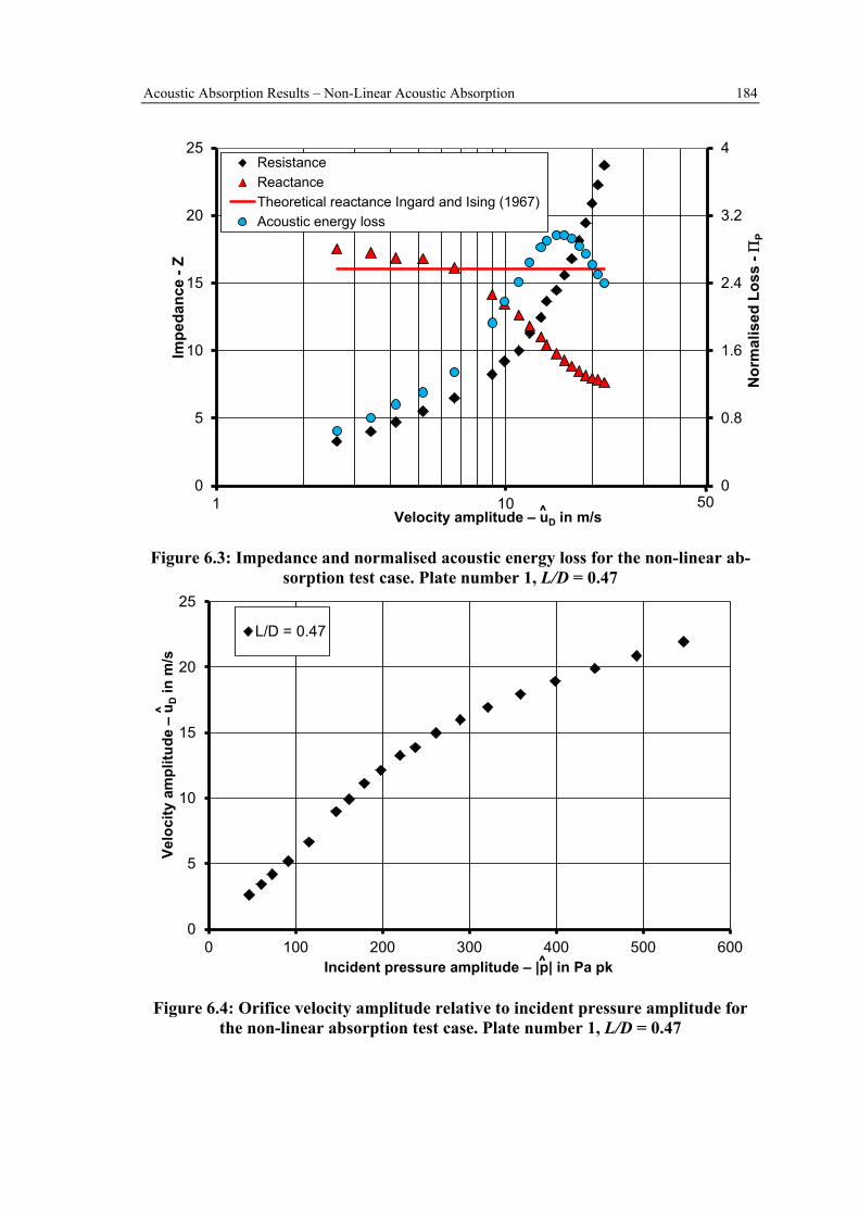
Acoustic Absorption Results – Non-Linear Acoustic Absorption 184
0
0.8
1.6
2.4
3.2
4
0
5
10
15
20
25
1 10
Nor
mal
ised
Los
s -Π
P
Impe
danc
e -Z
ResistanceReactanceTheoretical reactance Ingard and Ising (1967)Acoustic energy loss
50Velocity amplitude – uD in m/s^
Figure 6.3: Impedance and normalised acoustic energy loss for the non-linear ab-sorption test case. Plate number 1, L/D = 0.47
0
5
10
15
20
25
0 100 200 300 400 500 600
L/D = 0.47
Velo
city
am
plitu
de –
u Din
m/s
^
Incident pressure amplitude – |p| in Pa pk^
Figure 6.4: Orifice velocity amplitude relative to incident pressure amplitude for the non-linear absorption test case. Plate number 1, L/D = 0.47

Acoustic Absorption Results – Non-Linear Acoustic Absorption 185
0.0
0.1
0.2
0.3
0.4
0.5
0.6
0.7
115 120 125 130 135 140 145 150
Abso
rptio
n C
oeffi
cien
t ∆L/D = 0.5L/D = 1L/D = 1.5L/D = 2L/D = 2.4L/D = 3L/D = 5L/D = 6.8L/D = 10
Incident acoustic wave amplitude |p-| in dB^
Figure 6.5: Non-linear absorption coefficient for D = 9.1mm orifice at various L/D. Plate number 3 – 11, forcing frequency 62.5 Hz.
0
5
10
15
20
25
30
35
40
0 100 200 300 400 500 600 700
Impe
danc
e -Z
Re(Z) - L/D = 0.47
Im(Z) - L/D = 0.47
Re(Z) - L/D = 1.98
Im(Z) - L/D = 1.98
Incident pressure amplitude – |p| in Pa pk^
Figure 6.6: Impedance comparison for L/D of 0.47 and L/D of 1.98. Forcing fre-quency of 125 Hz. Plate number 1 and 13.

Acoustic Absorption Results – Non-Linear Acoustic Absorption 186
0
5
10
15
20
25
0 100 200 300 400 500 600 700
L/D = 0.47L/D = 1.98
Velo
city
am
plitu
de –
u Din
m/s
^
Incident pressure amplitude – |p| in Pa pk^
Figure 6.7: Non-linear absorption coefficient for various L/D. Plate number 1 and 13, forcing frequency 125 Hz.
0.0
0.1
0.2
0.3
0.4
0.5
0.6
0.7
0 2 4 6 8 10 12 14 16 18
Abso
rptio
n C
oeffi
cien
t ∆
L0/D
L/D = 0.5L/D = 1L/D = 1.5L/D = 2L/D = 2.4L/D = 3L/D = 5L/D = 6.8L/D = 10
Figure 6.8: Non-linear admittance dependent on vortex ring formation number for orifice length-to-diameter range of 0.5< L/D < 10. Plate number 3 – 11.

Acoustic Absorption Results – Non-Linear Acoustic Absorption 187
0
1
2
3
4
5
6
7
8
9
10
0 0.5 1 1.5 2 2.5 3 3.5
Vort
ex fo
rmat
ion
num
ber L
0/D
Orifice length-to-diameter ratio L/D
Figure 6.9: Vortex ring formation numbers at maximum absorption for a range of orifice length-to-diameter ratios. Plate numbers 3 – 8, 18 and 19.

Acoustic Absorption Results – Non-Linear Acoustic Absorption 188
Impedance Acoustic energy Loss
Plate number 19, L/D = 0.25
05
1015202530354045
0 1 2 3 4 5
Impe
danc
e -Z
L0/D
Measured reactanceMeasured resistanceModel reactanceModel resistance
Plate number 19, L/D = 0.25
0
10
20
30
40
50
0 1 2 3 4 5
Acou
stic
Los
s -Π
P
L0/D
ExperimentModel
x10-6
Plate number 22, L/D = 1
0
10
20
30
40
50
60
0 2 4 6 8 10
Impe
danc
e -Z
L0/D
Measured reactanceMeasured resistanceModel reactanceModel resistance
Plate number 22, L/D = 1
0
4
8
12
16
20
0 2 4 6 8 10
Acou
stic
Los
s - Π
P
L0/D
Experiment
Model
x10-6
Figure 6.10: Comparison between non-linear acoustic experiment and non-linear
acoustic absorption model

Acoustic Absorption Results – Non-Linear Acoustic Absorption 189
a) L/D = 0.5
0.0
0.1
0.2
0.3
0.4
0.5
0.6
0.7
120 130 140 150
∆
|p-| in dB
dp/p = 0%
dp/p = 0.1%
dp/p = 0.3%
dp/p = 0.5%
^
b) L/D = 1.98
0.0
0.1
0.2
0.3
0.4
120 130 140 150
∆
|p-| in dB^
c) L/D = 3
0.0
0.1
0.2
0.3
120 130 140 150
∆
|p-| in dB^
d) L/D = 6.8
0.0
0.1
0.2
120 130 140 150
∆
|p-| in dB^
Figure 6.11: Transition from linear to non-linear acoustic absorption, acoustic ab-sorption experiment, forcing frequency of 62.5 Hz. Plate numbers 3, 6, 8, 10.
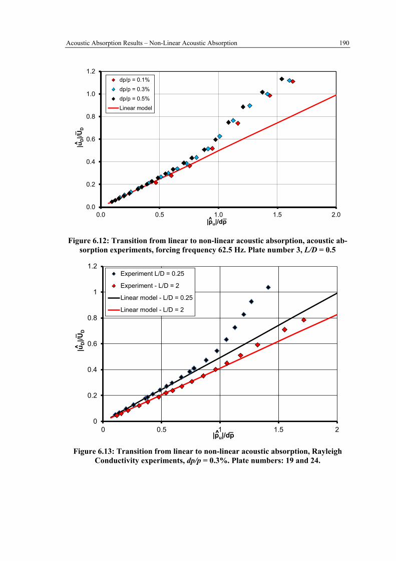
Acoustic Absorption Results – Non-Linear Acoustic Absorption 190
0.0
0.2
0.4
0.6
0.8
1.0
1.2
0.0 0.5 1.0 1.5 2.0
dp/p = 0.1%
dp/p = 0.3%
dp/p = 0.5%
Linear model
|uD|/U
D^
_
|pu|/dp^ _
Figure 6.12: Transition from linear to non-linear acoustic absorption, acoustic ab-
sorption experiments, forcing frequency 62.5 Hz. Plate number 3, L/D = 0.5
0
0.2
0.4
0.6
0.8
1
1.2
0 0.5 1 1.5 2
Experiment L/D = 0.25
Experiment - L/D = 2
Linear model - L/D = 0.25
Linear model - L/D = 2
|uD|/U
D^
_
|pu|/dp^ _
Figure 6.13: Transition from linear to non-linear acoustic absorption, Rayleigh
Conductivity experiments, dp/p = 0.3%. Plate numbers: 19 and 24.

Acoustic Absorption Results – Non-Linear Acoustic Absorption 191
0
5
10
15
20
25
30
35
40
45
50
0.0 2.5 5.0 7.5 10.0 12.5 15.0 17.5 20.0
Impe
danc
e Z
|uD|
Resistance - no flowReactance - no flowResistance - dp/p = 0.1%Reactance - dp/p = 0.1%
^
Figure 6.14: Impedance comparison during transition from linear to non-linear acoustic absorption with and without flow, forcing frequency 125 Hz. Plate num-
ber 19, L/D = 0.25.
0
5
10
15
20
25
30
35
40
45
50
0.0 2.5 5.0 7.5 10.0 12.5 15.0 17.5 20.0 22.5
Impe
danc
e Z
|uD|
Resistance - no flowReactance - no flowResistance - dp/p = 0.1%Reactance - dp/p = 0.1%
^
Figure 6.15: Impedance comparison during transition from linear to non-linear acoustic absorption with and without flow, forcing frequency 125 Hz. Plate num-
ber 24, L/D = 1.98.

Methodology to Identify Unsteady Flow Structures Associated with Acoustic Absorption 192
7 Methodology to Identify Unsteady Flow Struc-tures Associated with Acoustic Absorption
The amount of energy absorbed from the acoustic field is directly linked to various
features within the unsteady flow field in the vicinity of an orifice. Investigation of this
unsteady flow field will therefore provide a greater understanding of the relevant flow
field characteristics associated with the acoustic absorption process. An experimental
technique has been developed to enable interrogation of this region using Particle Image
Velocimetry (PIV) with adequate spatial and temporal velocity field information.
However, the mean pressure drop across the orifice will generate a mean flow field and
turbulence even in the absence of an acoustic pressure perturbation. Hence a data
analysis technique has been developed that identifies the unsteady features caused by
the incident acoustic pressure waves from other flow field features. This method is
based on the application of Proper Orthogonal Decomposition (POD). Initially an
introduction to the POD analysis will be given. Thereafter the developed methodology
is explained. This method will then be validated against the acoustic measurements
using the two-microphone method based on the acoustic absorption results shown in the
previous chapter. Finally the methodology is used to highlight fluid dynamic
phenomena leading to the absorption of acoustic energy within the linear and non-linear
acoustic absorption regime.
7.1 Introduction to the Proper Orthogonal Decomposition The Proper Orthogonal Decomposition, (POD) is a well-established method used for
structure identification within turbulent flow research, e.g. Adrian et. al. (2000), Bernero
and Fiedler (2000), Graftieaux et. al. (2001), Patte-Rouland et. al. (2001), Kostas et. al.
(2005), Midgley (2005), Robinson (2009),etc. In general the method is used to calculate
time averaged instantaneous velocity field data. The description of the used POD
analysis can also be found in Rupp et. al. (2010) and Rupp et. al. (2010b). In this work
before the Proper Orthogonal Decomposition is applied the time averaged flow field

Methodology to Identify Unsteady Flow Structures Associated with Acoustic Absorption 193
( ) ( ) ( )∑=
==N
1it,xu
T1
t,xuxu ( 7.1)
is subtracted from the data set. The symbol represents an ensemble average and N
denotes the amount of samples. Some authors do not subtract the mean flow field and
perform the POD method over the complete data set. In this case the first POD mode is
associated with the mean flow field However for this study the resulting data set
investigated in the Proper Orthogonal Decomposition is then defined by the
instantaneous fluctuating velocity vectors where the time average is
( ) ( ) ( ) 0t,xuN1
t,xuxuN
1iii =′=′=′ ∑
= ( 7.2)
and the time index is defined as Ni ,,1= , where N is the maximum amount of
samples, i.e. 3072.
The overall objective of the method is to extract time-independent orthonormal basis
functions (structural modes) ( )xkϕ and time dependent orthonormal coefficients
(temporal coefficients) ( )ik ta such that their reconstruction of the instantaneous velocity
field
( ) ( ) ( )∑=
⋅=′N
1kkiki xtat,xu ϕ ( 7.3)
is optimal. In this case the parameter k defines the POD mode number. This
reconstruction is optimal in the sense that it reconstructs the original data most
accurately from the first m < N sequential POD modes. The structural modes contain
information on the shape of the coherent structures within the fluctuating velocity field.
Each structural mode has a temporal coefficient which describes how the coherent
structure changes in time. A simple analogy is that the structural mode represents the
amplitude of a fluctuating velocity field associated with that mode, and the change of
this amplitude over time is represented by the temporal coefficient. Therefore the
temporal coefficient gives an indication of any coherent structures (or other features) in
the associated mode that are either periodic or of a random nature.

Methodology to Identify Unsteady Flow Structures Associated with Acoustic Absorption 194
Mathematical optimality is ensured by the maximisation of the averaged projection of
u′ onto ϕ (Holmes et. al. (1998)). Therefore, to satisfy the maximisation problem, ϕ
must be an eigenfunction of the two-point correlation tensor as discussed in Berkooz et.
al. (1993):
( ) ( ) ( )xxdxx,xRD
λϕϕ =′′′∫ . ( 7.4)
Thus the maximum is achieved for the largest eigenvalue λ. The integral is applied over
a spatial domain D. Moreover the spatial correlation tensor is represented by ( )'x,xR .
This spatial correlation tensor is a measure of the size of the structures within the flow
field and can also be used in calculating the integral length scales of the structures
within the flow field (e.g. Midgley (2005), Robinson (2009), Dunham (2011), etc).
To calculate the spatial correlation tensor the matrix A can be constructed containing
the fluctuating velocity components of the sampled planar PIV velocity field. In this
case the coordinate x resembles a pair of x and y coordinates, i.e. (x,y)i and m represents
the number of vectors within the flow field (m = 64×64 = 4096). It can be seen that the
spatial variation of the oscillating velocity vector is contained in the rows of the matrix
and its temporal variation within the columns of matrix A (e.g. Midgley(2005)):
( ) ( )
( ) ( )
′′
′′
=
Nmmm
N111
t,xut,xu
t,xut,xu
A
.
( 7.5)
Thereafter the spatial correlation function can be calculated ( )'x,xR :
( ) ( )TAAN
xxR 1=′, .
( 7.6)
As described in Sirovich (1987) the spatial POD modes can be calculated from the
eigenvectors of the spatial correlation matrix. Chatterjee (2000) showed that the spatial
modes can be inferred by using a Singular Value Decomposition (SVD):

Methodology to Identify Unsteady Flow Structures Associated with Acoustic Absorption 195
( ) TUx,xR ΣΦ=′ . ( 7.7)
In this case the large spatial correlation matrix is decomposed into three matrices: the
N×N matrix U, the m×m matrix Φ and the N×m matrix Σ. The matrix Σ consist of zero
elements except for the singular values along the diagonal elements of the matrix.
Furthermore the singular values are also ordered so that the first diagonal element is the
largest value. Moreover the columns of matrix Φ contain the eigenvectors. Therefore the
kth spatial POD mode can be extracted by using the kth column of the matrix Φ.
Calculating the spatial POD modes using the described method is computationally
expensive, as it is considering the m×m spatial correlation matrix ( )x,xR ′ . Thus, a
method proposed by Sirovich (1987), known as the Snapshot-POD method, was used.
In this case the SVD was conducted on the matrix C
( )TAAN
C 1=
( 7.8)
instead of the spatial correlation matrix R. Thus the elements in C are reduced to N×N
which reduces the computational effort as less time steps N are used than vectors in the
flow field m. However the Snapshot-method does not calculate the eigenvectors for the
spatial POD modes directly. In this case the eigenvectors κκ of the SVD need to be
multiplied with the matrix A containing the fluctuating velocity components:
( ) ( ) ( )∑=
=sN
1iiikk t,xAtx κϕ ( 7.9)
An important characteristic of the POD analysis is that the eigenvalue λi, which is the
square-root of the diagonal elements of matrix Σ, associated with a particular POD
mode divided by the sum of all eigenvalues of all POD modes is representative of the
kinetic energy contained in each mode relative to the total fluctuating kinetic energy.
∑
∑
=
==N
ii
k
ii
kE
1
1
λ
λ
.
( 7.10)

Methodology to Identify Unsteady Flow Structures Associated with Acoustic Absorption 196
Therefore the POD modes are ordered in terms of their kinetic energy. The first POD
mode contains the most energy averaged over the field of view. An example of the
cumulative kinetic energy distribution is shown in Figure 7.1. This data is based on a
acoustic flow field with 62.5 Hz excitation with 0.1% and 0.8% mean pressure drop. It
can be seen that the flow field at the smaller pressure drop contains an increased amount
of kinetic energy in the first POD modes.
The temporal variation of the spatial POD mode can be inferred from the unsteady
velocity field and the calculated spatial POD mode:
( )Tkk
Tkk ua ϕϕϕ′= . ( 7.11)
Thus the unsteady velocity field as defined in equation ( 7.3) can be reconstructed using
the temporal coefficient ak and the spatial modes ϕk.
The described POD method was implemented in the MATLAB routine Xact
developed by Robinson (2006). Velocity vectors calculated by the LaVision Davis 7.2
software were used as an input into the Xact analysis routine, which performed the
Snapshot-POD method on the unsteady velocity vectors.
The maximum amount of samples per test point for the represented test cases
specified by the high speed camera was 3072. At a sampling frequency of 1100 Hz this
results in 8 to 9 data points (i.e. velocity fields) per cycle for the excitation frequency of
125 Hz and 16 to 18 data points per cycle for the excitation frequency of 62.5 Hz. The
POD analysis was conducted on all 3072 data points. Due to the periodic signal this
resulted in 349 statistical independent samples for 125 Hz excitation and 174
independent samples for the 62.5 Hz excitation. Patte-Rouland et. al. (2001) mentions
that 400 statistical independent samples are sufficient for a good statistical
representation of the lower POD modes. Moreover it is shown that the cumulative
energy within the lower POD modes converge for a normalised mode number of k/N =
0.585, where k represents the mode number and N is the total number of snapshots.
Figure 7.2 shows the cumulative energy within the POD modes for examples of the
linear and non-linear acoustic absorption cases. It can be seen that the modes converge
around the same value of 0.585 with more than 99.9% of the cumulative kinetic energy.

Methodology to Identify Unsteady Flow Structures Associated with Acoustic Absorption 197
Hence the used amount of independent samples for this work seems sufficient for the
convergence of the amount of energy within the lower POD modes.
7.2 Methodology to Identify Unsteady Flow Structures Associated with Acoustic Absorption
The experimental investigation of the unsteady flow field was conducted using
particle image velocimetry (PIV). Various PIV velocity measurements have been
undertaken for the linear and non-linear absorption regime. The non-linear velocity
fields have been measured for plate number 1 (Table A.1) with 12.7 mm diameter and
L/D = 0.47. A small pressure drop across the orifice plate of 8 Pa has been applied to
drag the necessary seeding particles through the test section. The excited flow fields
have been measured at three different excitation pressure amplitudes (130 dB, 137 dB
and 142 dB) for the 125 Hz forcing cases. However to illustrate the developed
methodology the test point at 137 dB will be described in more detail. The absorption
measurement relative to the PIV test condition is also shown Figure 7.3 and suggests the
absorption is non-linear. Hence the reversing flow field is likely to generate vortex ring
type structures either side of the aperture, i.e. a significant amount of acoustic energy is
dissipated upstream of the orifice as well as downstream of the orifice. Thus two flow
field measurements at the same forcing amplitude have been conducted either side of
the orifice so that the vortex ring structures upstream and downstream of the orifice, due
to the reverse flow within the acoustic cycle, could be captured. The following
description of the methodology to identify the unsteady flow structures is taken from
Rupp et. al. (2010b).
The flow field chosen for the linear absorption regime was measured at 137 dB as
indicated in Figure 7.4. In this case the orifice diameter was 9.1 mm with a length-to-
diameter ratio (L/D) of 0.5 (plate number 3 in Table A.1) and an excitation frequency of
62.5 Hz. In the linear regime it is assumed that all the energy dissipation occurs within
the downstream flow field, hence no PIV measurements upstream of the aperture have
been captured. It should be noted that some of the energy could be dissipated within the
boundary layer internal to the orifice. However, due to the length of the investigated

Methodology to Identify Unsteady Flow Structures Associated with Acoustic Absorption 198
orifice plate the loss of acoustic energy, due to the boundary layer inside the orifice,
could be neglected (see chapter 5.9.1).
Figure 7.5 and Figure 7.6 show examples of the measured instantaneous flow fields
during non-linear and linear acoustic absorption. The total velocity is indicated in the
contour of both figures and stream traces have been added to show the characteristic of
the measured flow fields. Furthermore the Cartesian coordinates x and y have been
normalised using the orifice diameter. In Figure 7.5 two sequential instantaneous flow
fields within one acoustic cycle are shown for the flow field downstream of the orifice.
Figure 7.6 shows two sequential flow fields during linear absorption. At first glance
obvious differences within the flow fields are visible. It can be seen that the flow field
within the non-linear acoustic absorption regime shows large vortex ring structures
whereas the linear acoustic absorption regime is characterised by a pulsatile turbulent
jet. However, both flow fields are influenced by:
(i) the acoustic pressure oscillation producing the unsteady orifice pressure drop
(ii) the mean flow field which is caused by the centrifugal fan producing the
mean orifice pressure drop
(iii)almost random turbulent oscillations within the flow.
Thus a quantitative assessment of the coherent structures relevant to the acoustic
absorption may be possible if the fluctuating velocity could be decomposed into a
velocity field containing coherent, periodic structures (that correlate in some form with
the acoustic field and the incident acoustic pressure waves) and fluctuations that are
more random and turbulent in nature, (and which exhibit no correlation with the
acoustic field), i.e.
( ) ( ) ( ) ( )((
nsfluctuatioturbulentRandom
fieldvelocityperiodic
thebygeneratedstructuresCoherent
fieldflowMean
txutxuxutxu ..,',~, ++= ( 7.12)
Having decomposed the measured velocity field into these components an
instantaneous flow field can be reconstructed. For example, the reconstructed flow field
could include the mean flow field and periodic structures that exhibit coherence with the
Methodology to Identify Unsteady Flow Structures Associated with Acoustic Absorption 199
incident acoustic pressure waves (i.e. so that the random turbulent fluctuations are
ignored). In this way the reconstructed flow field and its subsequent analysis offers the
potential for identifying features generated by the incident pressure waves which are
responsible for absorbing energy from the acoustic field. However, careful
consideration is required as to how this analysis should be undertaken. This is because
as the flow field develops energy can, and will, be transferred between components. For
example, as the coherent structures in the flow field decay and mix out energy will be
transferred from these coherent structures into random turbulent fluctuations, whilst the
random turbulent fluctuations lose energy due to dissipation. In this work an attempt
was undertaken to decompose the unsteady velocity field using the Proper Orthogonal
Decomposition. This procedure is described in the following section which is based on
the data and methods described in Rupp et. al. (2010) and Rupp et. al. (2010b).
7.2.1 Flow Field Decomposition In general the methodology to identify the velocity field related to the acoustic
forcing relies on the analysis of the calculated POD modes based on the measured
unsteady velocity fields. All the POD modes have been calculated using the in-house
MATLAB routine Xact.
Figure 7.7 shows an example of three spatial POD modes calculated in the
downstream field within the non-linear absorption regime. Moreover the corresponding
temporal coefficients related to the spatial POD modes are shown in Figure 7.8. The
method to identify the acoustically related POD modes relies on an analysis of these
temporal coefficient. Thus, a Fourier transformation of the temporal coefficient was
conducted and is shown for the corresponding POD modes in Figure 7.9.
It can be seen that a large vortex structure is featured within POD mode 2 (Figure
7.7). Furthermore the temporal coefficient for this mode shows responses at the
excitation frequency of 125 Hz and its harmonics (Figure 7.9). In other words this
structure, and its associated energy, is strongly correlated with the incident pressure
wave. Similar behaviour can be seen from mode 4, which also shows vortex structures
within the spatial modes (Figure 7.7) and a frequency response in the temporal
coefficient at the excitation frequency (Figure 7.9). However in this case the 2nd and 3rd

Methodology to Identify Unsteady Flow Structures Associated with Acoustic Absorption 200
(250 and 375 Hz) harmonics seem to show a larger amount of energy than the
fundamental forcing frequency. Since the pressure spectrum does not show excitation
frequencies up to the third harmonic, the harmonics shown for mode 4 and mode 2 have
been generated in the flow field as a response to the 125 Hz excitation. This is expected
as it was also observed in the hotwire velocity measurements from Ingard (1960). A
mode representing random turbulent fluctuations is also presented (mode 100 in Figure
7.7 and Figure 7.9). It can be seen that no coherent structures are visible in the structural
mode and the temporal coefficients exhibit no significant response at the excitation
frequency (or its harmonics).
Moreover as another example the spatial modes, temporal coefficients and the Fourier
transforms of the temporal coefficients are shown in Figure 7.10 - Figure 7.12 for the
flow field within the linear absorption regime. In this case the shown POD modes are
representative of the pulsatile jet flow (e.g. mode 1 in Figure 7.10). Moreover no
structures seem to be visible in the vicinity of the aperture, i.e. y/D > -1, for mode 1 and
mode 3 (Figure 7.10). However the Fourier transformed coefficients (Figure 7.12) do
show evidence of the acoustic forcing frequency within their associated temporal
coefficients (in particular for modes 1 and 3). In this case almost no harmonic
frequencies at multiples of 62.5 Hz are visible. Finally random turbulent modes are also
shown, as for example for mode 100.
The periodic flow field related to the acoustic absorption can now be reconstructed
using only the modes which show a dominant frequency component in the temporal
coefficient which is either equal to the forcing frequency or a harmonic of that
frequency. This reconstruction of the flow field is detailed in the following section.
7.2.2 Flow Field Reconstruction In conventional flows the turbulent flow field is characterised by a range of turbulent
structures in which energy typically cascades from the large, energy containing, eddies
into smaller structures from which turbulent energy is dissipated into heat. Hence the
turbulent energy is distributed over a broad range of frequencies and gives rise to classic
spectra (e.g. Pope (2000)) in which the various sub-ranges can be identified (i.e. energy
containing range, non-viscous sub range, etc). Such a process would result in modes

Methodology to Identify Unsteady Flow Structures Associated with Acoustic Absorption 201
whose temporal coefficients exhibit no preferred frequencies (e.g. mode 100 in Figure
7.9 and Figure 7.12). However, as already shown some modes exhibit temporal
coefficients which suggest the velocity field, associated with that mode, has a preferred
frequency of fluctuation that corresponds to the acoustic excitation frequency (or its
harmonic). Hence this suggests that the velocity field associated with this mode, and its
associated flow field features, has been generated by the incident acoustic pressure
waves. In other words the energy associated with this mode has, potentially, originated
from the acoustic field and therefore represents the mechanism by which energy is
being absorbed from the incident acoustic waves.
A filter routine was developed which identifies modes whose temporal coefficients
exhibit preferred frequencies at the excitation frequencies, or its harmonics, such as that
indicated by modes 2 and 4 (Figure 7.9) or modes 1 and 3 (Figure 7.12). The function of
the filtering is illustrated in Figure 7.13 with the spectrum of the temporal coefficient of
mode 2 in the non-linear absorption example. The routine is averaging all the
amplitudes within the spectrum. Furthermore the maximum amplitude and its frequency
are also identified. The frequency at which the maximum amplitude occurs must lie
within a frequency band ∆f of ±1% of the excitation frequency or its harmonics so that
the mode is considered as an acoustically related mode. Finally the amplitude within the
frequency band has to be at least two times larger than the averaged amplitude of the
spectrum.
Applying the filter to the data set resulted in approximately 140 modes, out of the
possible 3072 modes, being identified within the flow field of the non-linear absorption
regime. Furthermore 720 modes have been identified within the flow field in the linear
absorption regime. Figure 7.14 shows the cumulative energy distribution for the POD
modes in the non-linear regime. The diamonds which coincide with the cumulative
energy curve symbolise the filtered POD modes used by the reconstruction of the flow
field. The diamonds which coincide with 0% cumulative energy indicate that these
modes were not used. The same can be seen from Figure 7.15 for the measurement in
the linear acoustic absorption regime. It can be seen that 9 out of the 10 first POD
modes were used in the non-linear regime (Figure 7.14). Moreover these modes equate
to 90% of the total kinetic energy of the oscillating flow field. For the linear regime

Methodology to Identify Unsteady Flow Structures Associated with Acoustic Absorption 202
only 5 of the first 10 POD modes are used (Figure 7.15). Moreover comparing both
cumulative energy curves it can be seen that more oscillating kinetic energy is contained
within the first 10 modes relative to the total kinetic energy within the non-linear
absorption regime. This is implying that the linear absorption regime case is dominated
by smaller scale structures containing less of the total energy within the flow field
compared to the non-linear absorption case.
The filtered POD modes are referred to as the ‘acoustically related’ modes and the
flow field was then reconstructed using only these modes. This reconstructed velocity
field is thought to represent the unsteady flow field generated by the acoustic pressure
fluctuations. The remaining modes can also be reconstructed and this, of course,
represents the random turbulent field. This flow field is associated with, for example,
the mean flow and the turbulence generated as it passes through the orifice. In this way
the instantaneous velocity field components defined in equation ( 7.12) could be
identified and the associated flow fields reconstructed.
The power spectral density for the v-velocity component has been used to initially
assess the velocity field of the acoustically related modes with respect to the total
velocity field and the turbulent field. The turbulent field was reconstructed from the
modes which were rejected by the filter function. Two points within the non-linear
acoustic flow field, as indicated in Figure 7.16, were used for this analysis. In this case
the total velocity was shown as a contour within the flow field and the orifice is located
at y/D = 0. Point 1 was located on the centreline of the unsteady jet flow (x/D = 0 and
y/D = -0.4) and point 2 was located within the shear layer of the pulsatile flow field (x/D
= 0.4 and y/D = -0.6). The power spectral density for point 1 is shown in Figure 7.17.
Spectra are presented for the total velocity field and the velocity fields reconstructed
from the ‘acoustically related’ and ‘turbulent related’ POD modes identified by the filter.
It can be seen that all the energy contained in the spectra at 125 Hz and its harmonics
has been captured in the filtered flow field reconstructed from the ‘acoustic related’
modes. Alternatively the reconstructed velocity field from the ‘turbulent related’ modes
has its energy distributed over a broad frequency range (as required). Similar behaviour
can be seen for different regions of the flow field, such as in the shear layer region at the
edge of the unsteady jet (point 2) as shown in Figure 7.18. These results suggest the

Methodology to Identify Unsteady Flow Structures Associated with Acoustic Absorption 203
methodology has been successful in identifying the coherent structures and other
features that are generated by the incident acoustic pressure waves.
The same filter has been applied to the POD modes of the flow fields within the linear
absorption regime, e.g. Figure 7.10 - Figure 7.12. Again two points within the unsteady
flow field are chosen (Figure 7.19) to assess the effectiveness of the filter routine. The
power spectral densities of point 1, on the centreline of the jet, and point 2, within the
shear layer of the jet, are shown in Figure 7.20 and Figure 7.21. It can be seen that all
the periodic components within the power spectral densities has been filtered out of the
total velocity flow field for both cases. Moreover the turbulent fluctuations within the
flow field have been minimised within the periodic acoustically related flow field.
Hence the filter function was capable of filtering the relevant periodic coherent POD
modes.
Comparison of Raw and Reconstructed Flow Field – Non-Linear Absorption Regime
The flow field reconstructed on the downstream side of the orifice, using the ‘acoustic
related’ modes, is shown for various phases of the acoustic cycle in comparison to the
raw velocity field (Figure 7.22) for the non-linear absorption regime. Moreover the
phase angle of the acoustic oscillation, streamtraces to highlight the vortex rings within
the flow field as well as the contour of the unsteady velocity magnitude are included in
the figures. It can be seen that the incident acoustic waves generate an unsteady pressure
drop across the orifice which leads to the pulsation of flow through the orifice. As fluid
issues from the orifice it rolls up to form a vortex ring structure. The vortex ring
structure then induces a flow field through the centre of the ring propelling the structure
away from the aperture. It can be seen that most of the random turbulent velocity
oscillations have been suppressed in the reconstructed acoustically related velocity field
compared to the raw velocity field which is further encouragement that the filter method
for the acoustically related modes is working in the non-linear absorption regime.
Comparison of Raw and Reconstructed Flow Field – Linear Absorption Regime
Figure 7.23 shows the reconstructed acoustically related flow field in comparison to the
raw velocity field for the example in the linear regime. Note that the mean flow field is
included in the acoustically related field as well as in the raw velocity field for

Methodology to Identify Unsteady Flow Structures Associated with Acoustic Absorption 204
comparison. The contours of the velocity magnitude together with streamtraces to
highlight the flow field characteristic are shown in the figures. In this case two
instantaneous flow fields near the maximum velocity within the acoustic cycle are
shown. A pulsatile jet flow is visible which develops a shear layer at the edge of the
orifice. Again comparing the raw velocity field with the acoustically related flow field
shows that the majority of the random turbulent velocity oscillations have been filtered
out just leaving the oscillating jet flow. Hence the filter routine is operating as intended
within the linear absorption regime.
7.2.3 Validation of the Unsteady Flow Field Methodology A further validation of the method has been conducted comparing the acoustic energy
loss (derived from the pressure measurement) to the kinetic energy captured within the
acoustically related flow field. For the described method to be valid the calculated
energy loss for both cases has to agree. The validation within the linear and non-linear
regime is described in detail in appendix C or in Rupp et. al. (2010b). However a brief
overview of the energy loss calculation and the validation results is shown in this
section.
The loss of acoustic energy derived from the pressure measurements can be calculated
based on the acoustic energy fluxes as shown in equations (5.1) to (5.3). Moreover the
unsteady energy flux measured from the filtered acoustically related unsteady velocity
field can be derived using the unsteady energy flux of the jet flow:
221 vmE = . ( 7.13)
The detailed energy flux calculation performed on the acoustically related flow field is
described in appendix C.
Figure 7.24 shows the comparison between the acoustic energy loss and the kinetic
energy flux derived from the unsteady flow field for an example in the non-linear and
the linear acoustic absorption regime. It can be seen that the kinetic energy flux derived
from the acoustically related flow field agrees very well with the measured acoustic
energy loss for both the linear and non-linear regime. As it can be seen in the non-linear
absorption regime only a small amount of the kinetic energy originates from the mean

Methodology to Identify Unsteady Flow Structures Associated with Acoustic Absorption 205
flow field. Hence the total velocity field and the acoustically related flow field show
very similar kinetic energy fluxes. However, as is shown for the linear case, the mean
flow field and the associated random turbulent portion show a much larger acoustic
energy flux compared with the acoustic measurement and the filtered acoustically
related velocity field. This shows the importance of the method for the cases where the
influence of energy sources other than the acoustic energy sources are large. In general
the method agrees very well with the acoustic absorption measurement. Therefore the
data suggests that the relevant acoustic flow field has been captured and the method is
valid.
7.3 Characteristics of the Unsteady Velocity Field Related to Acoustic Absorption
As the flow field analysis technique has been validated using the data measured from
the acoustic experiments it is now possible to investigate the flow field features
associated with the acoustic absorption behaviour in more detail.
7.3.1 Non-Linear Absorption Regime As discussed in the previous sections the non-linear acoustic absorption regime is
characterised by large scale vortex rings. The interaction of the large scale structures
with the unsteady jet flow is thought to be the main influence on the acoustic absorption
characteristics described in chapter 6. For example Figure 7.25 shows a comparison of
the mean velocity field between the unforced flow field (no acoustic excitation) and the
forced flow field (137 dB excitation). In the unforced case a steady jet flow entering and
exiting the aperture is visible. This is very different in the case with acoustic excitation.
The generated vortex ring structures upstream and downstream of the orifice induce a
velocity field through the centre of the vortex ring which is directed away from the
aperture. In this way the vortex rings are propelled further downstream from the
aperture. The induced flow field generated by the vortex rings produces a mean flow
field which is significantly different to the mean flow field without acoustic excitation.
Hence the unsteady flow field and the influence of the vortex ring structures have been
investigated further in this section.

Methodology to Identify Unsteady Flow Structures Associated with Acoustic Absorption 206
Prior to discussing the unsteady flow field in more detail some important parameters
are introduced. The velocities shown in this section have been non-dimensionalised
using the mean blowing velocity (e.g. Jabbal et. al. (2006))
( )∫=2
0
1 T
bulkblow dttUT
U . ( 7.14)
In this case the blowing velocity represents the outflow velocity into the downstream or
upstream flow field integrated over half an acoustic cycle. Moreover the bulk velocity
Ubulk is defined as the area averaged v-velocity component at the downstream exit of the
aperture (e.g. Jabbal et. al. (2006))
( ) ( ) ( )∫==R
DDbulk drrtrv
AAtmtU
0
2,
πρ
. ( 7.15)
Another important parameter is the generated vorticity of the unsteady jet flows. The
measured planar flow fields consist of u and v-velocity components; hence the vorticity
in the z-direction can be considered (equation 2.7)
yu
xv
z ∂∂
−∂∂
=R . ( 7.16)
The measured flow field is i and j ordered for the x and y coordinate directions. Thus the
first order differential operators in the vorticity equation ( 7.16) have been defined using
the least squares method as defined in Raffel et. al. (1998):
( )( )
( ) ( ) ( ) ( )y
jiujiujiujiujiyjiu
∆−−−−+++
≈∂∂
10221122 ,,,,
,, . ( 7.17)
The same differential operator was used on the v-velocity derivative. Furthermore at the
edges of the flow field less accurate forward and backward differences are applied. In
this case the vorticity has been non-dimensionalised using the mean blowing velocity of
the unsteady jet case
DUblowz
NR
R = . ( 7.18)

Methodology to Identify Unsteady Flow Structures Associated with Acoustic Absorption 207
Similar vorticity normalisations have been defined by other authors, e.g. Krueger et. al.
(2006) and Aydemir et. al. (2012).
As shown in the previous section the measured acoustic energy loss agrees very well
with the kinetic energy present in the unsteady flow field. The method by which the
kinetic energy of the unsteady flow field was calculated provides an insight into the
energy transfer that occurs within the flow field. In the non-linear regime two methods
can be used to estimate the energy within the flow field upstream and downstream of
the orifice.
i) An integration was used over a cylindrical volume (see Figure 7.26 (a)) to
estimate the kinetic energy within the flow field. The calculation of the kinetic
energy in the unsteady flow field was based on the method proposed by Tam and
Kurbatskii (2000). This method captures the kinetic energy contained within the
vortex ring structure and the pulsatile jet flow.
ii) The kinetic energy flux of the upstream flow field was calculated in the plane
immediately upstream and downstream of the orifice (example of downstream
surface is shown in Figure 7.26 (b)). In this case only the kinetic energy flux of
the pulsatile jet flow is represented.
Figure 7.27 shows a comparison between (i) the two kinetic energy calculation
methods derived from the acoustically related flow field and (ii) the measured acoustic
energy loss from the acoustic experiment The detailed definition for both methods can
be found in appendix C. As can be seen both methods agree very well within the
accuracy of the experiments. To investigate the energy transfer further the measured
velocity fields have been phase averaged as described in appendix D. The phase
averaged data was then used to calculate the kinetic energy of the pulsatile flow and the
vortex ring in the flow field at various time steps throughout the acoustic cycle.
Figure 7.28 shows the calculated kinetic energy in the downstream field of view as
well as the v-velocity component on the centreline immediately downstream of the
aperture. The kinetic energy in Figure 7.28 has been normalised using the maximum
kinetic energy calculated within one acoustic cycle. Furthermore the velocity has been
normalised using the mean blowing velocity as described in ( 7.14) It can be seen that

Methodology to Identify Unsteady Flow Structures Associated with Acoustic Absorption 208
the kinetic energy of the pulsatile flow field is increasing up to a maximum at t/T =
0.34. Thereafter the kinetic energy is reducing. The presented data can be used to
estimate the transfer of kinetic energy from the pulsatile jet into the kinetic energy of the
vortex ring. During the outflow of fluid into the downstream control volume the sign of
the velocity is negative. During the inflow phase (i.e. change of flow direction from
downstream to upstream) where the velocity changes sign no further kinetic energy flux
will be transferred into the downstream flow field. As Figure 7.29 shows the vorticity
field for the 131 dB forcing at the time step t/T = 0.57 does only show the vortex ring
and the induced flow field through the centre of the ring vortex. Hence the kinetic
energy at time step t/T = 0.57 can be used to estimate the kinetic energy of the vortex
ring structure (identified with a red line in Figure 7.28). In this case approximately 73%
of the maximum kinetic energy within the flow field has been transferred to the vortex
ring structure. The same approach was used for the 137 dB excitation case and
approximately 86% of the maximum kinetic energy in the flow field was transferred to
the vortex ring. For the 142 dB excitation case the vortex ring energy could not be
estimated as parts of the ring vortex travelled already outside the field of view (Figure
7.29). This shows that the acoustic excitation generates an unsteady jet flow across the
aperture. Parts of the kinetic energy of this pulsatile jet flow is converted into the kinetic
energy of large scale vortex rings and parts of the energy being dissipated in the shear
layers of the pulsatile jet.
The non-linear acoustic absorption coefficient for the investigated flow fields was
shown in Figure 7.3. The changes in acoustic reactance and resistance have been
discussed in the previous section. However it is apparent that the phase angle between
the pressure amplitude incident onto the aperture and the velocity amplitude within the
aperture is reducing with increasing excitation pressure amplitude due to the discussed
reduction in acoustic reactance with increasing pressure amplitude (section 6.1). This is
indicated in the acoustic experiment as shown in Figure 7.30. The phase averaged
centreline velocities of the acoustically related flow field downstream of the aperture is
also shown in Figure 7.31 for the three forcing cases. Unfortunately the velocity
measurements have not been synchronised with the pressure measurement. However, as
the PIV measurement has been triggered off the function generator for the loudspeaker

Methodology to Identify Unsteady Flow Structures Associated with Acoustic Absorption 209
signal it can be expected that the PIV measurement was taken at the same phase
location of the acoustic cycle. Hence the relative phase of the oscillating velocity field
with increasing incident pressure amplitude can be assessed. The example in Figure
7.31 shows that the maximum downstream centreline velocity for three different
acoustic pressure amplitudes occurs at an earlier time within the acoustic cycle for
increasing excitation pressure amplitudes. This is indicative of a reduction in phase
angle between the pressure amplitudes and velocity amplitudes and agrees with the
measured acoustic data.
The explanation for this shift in frequency can be found by investigating the location
of the vortex ring relative to the aperture. This has been conducted for the example of
the downstream velocity field in Figure 7.32. The total velocity contours as well as
stream traces are shown for the three excitation cases. Note for convenience the total
velocity contour has been normalised with the mean blowing velocity. The three forcing
cases are shown at the point where the flow direction changes from the downstream
flow field into the upstream flow field. It can be seen that the direction of the centreline
velocities at the orifice exit (x/D = 0 and y/D = 0) are still pointing into the downstream
flow filed. However at the aperture edges (-0.5 < x/D < -0.3 and 0.3 < x/D < 0.5 at y/D =
0) inflow into the aperture occurs with stream traces pointing into the upstream flow
field. It can be seen that for the small forcing amplitude of 131 dB the vortex ring
remains in the direct vicinity of the aperture (i.e. y/D ~ 0.6). The cases with larger
excitation amplitude show the location of the vortex ring further downstream (i.e. y/D ~
1.4 for 137 dB excitation and y/D ~ 142 dB excitation). In these cases the larger kinetic
energy of the vortex ring together with the higher unsteady jet velocity has propelled the
structure further away from the orifice. As the ring remains in the vicinity of the
aperture for the small excitation cases it is acting as an additional blockage for the flow
to pass through the aperture during the change in flow direction. In this case the inflow
to the aperture needs to flow around the structure and therefore more time is needed for
the fluid to get through the aperture. The further the ring vortex structure is away from
the orifice the smaller is the interaction with the incoming fluid to the aperture and
therefore the phase between the pressure oscillation and the velocity oscillation reduces.

Methodology to Identify Unsteady Flow Structures Associated with Acoustic Absorption 210
This phenomenon explains the reduction in the measured acoustic reactance for the
aperture.
Overall it can be concluded that the change in the acoustic impedance, i.e. the
decrease in reactance with increasing pressure amplitude, as described in the previous
chapter, is caused by the characteristics of the generated vortex ring structure within the
non-linear acoustic absorption regime. The changes in the acoustic quantities are
controlled by the interaction between the unsteady jet flow and the vortex ring
structures. The pulsatile jet seems to supply the energy for the vortex ring structures as
indicated by kinetic energy within the flow field and the energy flux across the aperture.
Moreover the vortex ring interacts with the fluid flowing in and out of the aperture
during the change of sign in the acoustic forcing cycle. Therefore the changes in the
measured acoustic impedance and ultimately the acoustic absorption are directly related
to the interaction between vortex rings and the pulsatile jet flow and thus to the location
of the ring relative to the orifice. Hence a better understanding of this behaviour would
improve the non-linear modelling techniques. Therefore the developed methodology
could aid in further detailed unsteady flow investigations in the non-linear acoustic
absorption regime.
7.3.2 Linear Absorption Regime In this section the acoustically related flow field during linear acoustic absorption is
investigated. Figure 7.33 shows the phase averaged v-velocity contour on the centreline
(x/D = 0 and y/D = -0.07) of the orifice within the downstream flow field for an orifice
with L/D = 0.5 at dp/p = 0.8% as well as L/D = 1 at dp/p = 0.3%. Three components of
the acoustically related velocity field are shown in both graphs: the acoustically related
flow fields including mean flow and all relevant POD modes, POD mode 1 including
the mean flow field and POD mode 1 only. It can be seen that the velocity oscillation on
the centreline can be reproduced using POD mode 1 including the mean flow only.
Moreover the first POD mode also contains 77% of the kinetic energy flux, which also
accounts for 77% of the total acoustic energy loss. Hence this could be seen as the most
dominant mode in the flow field. Hence the linear flow field and in particular the first
POD mode will be investigated in this section.

Methodology to Identify Unsteady Flow Structures Associated with Acoustic Absorption 211
Figure 7.34 shows the phase averaged acoustically related flow field including mean
flow for four instances during the acoustic cycle. In this case the flow fields for an
orifice of L/D = 0.5 at dp/p = 0.8% pressure drop was investigated. However, this flow
field is representative of the characteristics for all the investigated flow fields within the
linear regime for Strouhal numbers below 0.2. The orifice location is also indicated at
the top of the downstream flow field at -0.5 < x/D < 0.5 and y/D = 0. The flow field is
indicating a pulsatile jet flow with no visible significant flow structures such as eddies
or vortex rings. This is expected for a flow field associated with the linear acoustic
absorption as described in chapter 5.
However the flow field and its pulsatile nature can be further investigated showing
POD mode 1, which is seen as the dominant mode within the linear acoustic absorption.
Figure 7.35 shows the total velocity contours of POD mode 1 for L/D = 0.5 and dp/ p =
0.8% during linear acoustic absorption. Four instances along the acoustic cycle are
shown together with the velocity vectors. The length of each vector is scaled relative to
the velocity contour. No mean flow is present within the POD mode and hence the
velocity contour is changing sign from negative maximum velocity at t/T = 0.02 to 0 at
t/T = 0.2 and maximum positive velocity at t/T = 0.5. As could have been expected from
the quasi-steady investigation in chapter 5.5, the linear acoustic absorption is dominated
by a pulsatile flow field. This flow field subsequently decays into smaller scale
structures as for example shown in Figure 7.36 which ultimately decay within the
turbulent field of the jet. The structures indicated in Figure 7.36 do not seem to
influence the pulsatile jet flow field as they are not visible within the acoustically
related field of Figure 7.34. It can be assumed that these structures are part of the energy
dissipation process in the flow field (following the cascade processes as described for
example in Pope (2000)). Moreover an example of a forced and unforced mean jet flow
within the linear absorption regime is shown in Figure 7.37. There is no significant
difference between the forced and unforced jet visible. Therefore it can be concluded
that the unsteady flow field characteristics do not influence the mean flow field.
The measurements indicate that linear acoustic absorption at gas turbine combustion
system Strouhal numbers is associated with pulsatile, quasi-steady flow. In these cases
the acoustic length correction and the steady state discharge coefficient remain constant,

Methodology to Identify Unsteady Flow Structures Associated with Acoustic Absorption 212
i.e. chapter 5.9.1, which seems to be indicative that the unsteady flow structures
produced are not large enough to influence the pulsatile flow field of the orifice. Hence
simple one-dimensional models with representative steady state discharge coefficient
and constant length correction simulating the oscillating mass of the aperture flow field
are adequate. The flow field studies seem to be only required in areas where the linear
acoustic absorption is affected by unsteady flow structures within the flow field.
However a useful application of the described method would be the investigation of the
unsteady flow field within an aperture with large L/D ratio. As chapter 5 has shown this
is still a challenging area for a linear absorption model. Hence the application of the
method to CFD simulations or more sophisticated measurements within the aperture
would have the potential to improve the accuracy of the analytical modelling technique.
7.3.3 Transition from Linear to Non-Linear Absorption Another purpose for the developed methodology is the transition from linear to non-
linear absorption. As described in chapter 6.4 this is an important part for acoustic
dampers designed for gas turbine combustors. As amplitudes increase and the
absorption transitions from linear to non-linear acoustic absorption the relationship
between pressure and velocity oscillation changes from linear to non-linear. The
accurate prediction of the velocity amplitude is not only important for an accurate
absorption prediction but also the assessment of hot gas ingestion into the damper
geometry. The modelling aspects of the transition was described in Chapter 6.4.3 and it
was highlighted that this is a challenging task and heavily reliant on empirical data.
Unfortunately only limited data has been recorded for the unsteady flow field
investigation within the transition region. Nevertheless the developed methodology was
used to show some of the relevant unsteady flow features.
Figure 7.38 shows the acoustic absorption measurements for two orifice plates at two
mean pressure drops. Moreover for each orifice plate two PIV measurements have been
conducted. It can be seen that the PIV flow field measurement for the cylindrical orifice
with L/D = 0.5 and the conical orifice at a mean pressure drop of dp/p = 0.3% is within
the linear acoustic absorption regime as indicated by constant absorption coefficients for
increasing excitation pressure amplitudes. Moreover the PIV measurement for both
orifice plates at reduced pressure drop of 0.1% is within the transition region to non-

Methodology to Identify Unsteady Flow Structures Associated with Acoustic Absorption 213
linear acoustic absorption. Thereby the cylindrical orifice is located closer to the onset
of non-linear absorption whereas the test condition for the conical orifice plate is further
within the transition region of non-linear absorption.
The phase averaged normalised total velocity contours for the cylindrical orifice are
shown in Figure 7.39 together with the spectrum of the v-velocity component for the
two mean pressure drops at x/D = 0 and y/D = -0.26. It can be seen that the phase
averaged velocity for the dp/p = 0.3% case is looking more like a sine-wave whereas the
phase averaged normalised velocity trace is distorted indicating the occurrence of
harmonics. This is confirmed by the Fourier transformation of the v-velocity component
on the centreline of the orifice from the acoustically related flow field. In both cases the
first harmonic of 125 Hz is visible. However in the non-linear absorption case the
harmonic is larger. Moreover higher order harmonics are also visible. The velocity
amplitude ratio calculated using the v-velocity amplitude on the centreline of the orifice
and the time averaged v-velocity component at the same location is measured as 0.19
for the linear absorption case and 0.39 for the transition to non-linear acoustic
absorption case (which is in agreement with the velocity amplitude ratio shown in
chapter 6.4.1). The same behaviour can be seen for the conical orifice plate with 45°
cone angle as shown in Figure 7.40. Again the phase averaged normalised velocity is
shown for the linear and non-linear case as well as a Fourier spectrum of the centreline
velocity. Again the velocity amplitude for the linear case is measured as 0.27 and 0.6 for
the non-linear case. However in this case the onset of higher order harmonics (3rd and
4th) is already shown in the velocity spectrum for the dp/p = 0.3% case. This is due to
the increased velocity amplitude and the vicinity to the onset of non-linear absorption
which is also shown in Figure 7.38 for the dp/p = 0.3% case.
The acoustically related normalised total velocity field for cylindrical orifice of L/D =
0.5 and dp/p = 03% is shown in Figure 7.41. In general this pulsatile jet flow is very
similar to the one shown earlier for the linear regime, e.g. Figure 7.34. Moreover the
streamtraces of the velocity fields are shown to highlight any occurring flow structures.
It can be seen that there are no significant unsteady flow structures visible affecting the
unsteady flow field.

Methodology to Identify Unsteady Flow Structures Associated with Acoustic Absorption 214
Figure 7.42 shows the phase averaged normalised total velocity contours for the
acoustically related flow field associated with the onset to non-linear acoustic
absorption. In this case the mean pressure drop was 0.1% and the cylindrical orifice
with L/D = 0.5 was investigated. The three flow fields represent phases within the
acoustic cycle which clearly show the development of a vortex structure within the flow
field during the pulsatile outflow cycle for t/T > 0.5.
The influence of the vortex ring structure is also clearly visible in Figure 7.43 where
the acoustic forcing is much further into the non-linear absorption regime. This flow
field is looking very similar to the flow field shown in the non-linear absorption cases,
e.g. Figure 7.22.
The captured data suggests that the occurrence of vortex rings is related to the
transition to non-linear acoustic absorption. No significant large scale flow structure is
visible within the data captured during the linear acoustic absorption. However at the
onset of non-linear acoustic absorption the occurrence of higher order harmonics in the
velocity field become visible. The harmonics in the spectrum are most likely produced
by the occurrence of large scale flow structures which are interacting with the unsteady
flow field. Thus the transition from a linear relationship between pressure and velocity
to a non-linear relationship is caused by the change from a pulsatile flow field without
flow structures to the pulsatile flow field influenced by large scale vortex ring
structures.
7.4 Closure In this chapter an analysis technique has been developed which enables the
identification of the unsteady flow field associated with the acoustic absorption. This
method was based on POD analysis and an adequate filter function for the identification
of the acoustically related POD modes. In this case the method has been applied to PIV
measurement data. Nevertheless the methodology could also be applied to any velocity
field prediction or measurements with adequate temporal or spatial resolution. The
method has been successfully validated against the measured acoustic energy loss based
on the data described in chapter 5 and 6. For all the investigated flow fields the kinetic
energy flux of the acoustically related flow field was in very good agreement with the

Methodology to Identify Unsteady Flow Structures Associated with Acoustic Absorption 215
measured acoustic energy loss from the two-microphone measurements. Moreover the
method has shown its potential in identifying relevant mechanism to describe the
acoustic absorption behaviour of the investigated orifice plates in the linear and non-
linear absorption regime as well as in the transition region from linear to non-linear
acoustic absorption.
For example the investigation into the flow field during non-linear acoustic
absorption has shown that observed changes in acoustic absorption and acoustic
impedance reflect the fluid dynamic characteristics of the generated large scale vortex
ring structures. It was found that the unsteady kinetic energy flux across the aperture
agree with the amount of acoustic energy absorbed. Furthermore it was shown that a
significant amount of this energy flux is transferred into the kinetic energy of vortex
ring structures. These vortex rings interact with the mean flow field as well as with the
unsteady pulsatile flow field. It was shown that the reduction in acoustic reactance is
due to the increasing distance between the vortex ring and the orifice for increasing
pressure amplitudes. At small amplitudes the large scale structure remains in the vicinity
of the aperture and acts as an additional blockage for the flow into the aperture. As the
amplitudes are increased the ring vortex is propelled further away from the aperture.
Hence the additional blockage is reduced enabling the fluid to pass through the orifice
without having to flow around the ring structure. Thus the ring vortex interacts less with
the inflow into the aperture and the phase between pressure and velocity amplitudes
reduces. Furthermore the measured flow fields also show that large scale ring vortices
occur at the onset of non-linear acoustic absorption.
The flow field for the linear acoustic absorption regime has shown no significant
unsteady flow structures within the flow field. In this case the unsteady flow field is
dominated by a pulsatile jet flow for the operating conditions investigated. Hence the
acoustic absorption mechanism is an energy transfer from the acoustic field into the
kinetic energy of the unsteady jet. Ultimately kinetic energy of the flow field is
dissipated by turbulence. It seems as if a flow field investigation is less important for
the linear flow field within the considered Strouhal number range of relevance to this
investigation. However for technical applications with higher Strouhal numbers this
method could be used to identify the unsteady flow phenomena.

Methodology to Identify Unsteady Flow Structures Associated with Acoustic Absorption 216
The developed method could be applied to CFD simulations or experimental
measurements of the unsteady flow. In this way the influence of the optimum vortex
ring formation upon the optimum acoustic absorption with changing length-to-diameter
ratios could be further assessed. Moreover the method could also be used to investigate
the linear absorption regime and the unsteady flow within long apertures with L/D
larger two. In this way the unsteady flow analysis could be used to improve the current
analytical modelling assumptions.

Methodology to Identify Unsteady Flow Structures Associated with Acoustic Absorption 217
Figures
0
20
40
60
80
100
120
0 200 400 600 800 1000 1200 1400 1600
Cum
ulat
ive
kine
tic e
nerg
y in
%
POD mode number k
dp/p = 0.8%
dp/p = 0.1%
Figure 7.1: Example of cumulative kinetic energy within POD modes for the data
set at 0.8% dp/p and 135 dB excitation amplitude, plate number 3.
0
20
40
60
80
100
120
140
0.0 0.2 0.4 0.6 0.8 1.0
Cum
ulat
ive
kine
tic e
nerg
y in
%
k/N
Non-linearLinearconvergence - 0.585
Figure 7.2: Example of convergence of cumulative energy for example POD modes

Methodology to Identify Unsteady Flow Structures Associated with Acoustic Absorption 218
0.0
0.1
0.2
0.3
0.4
0.5
0.6
115 120 125 130 135 140 145
Abso
rptio
n co
effic
ient
-∆
Excitation amplitude in dB
Acoustic measurement
PIV data points
Figure 7.3: PIV data points relative to measured absorption coefficient curves,
non-linear acoustic absorption, L/D = 0.47, f = 125 Hz, plate number 1.
0.00
0.05
0.10
0.15
0.20
0.25
0.30
136 138 140 142 144 146 148
Abso
rptio
n co
effic
ient
-∆
Excitation amplitude in dB
Acoustic measurement
PIV data point
Figure 7.4: PIV data points relative to measured absorption coefficient curve, line-
ar acoustic absorption, L/D = 0.5, f = 62.5 Hz, 0.8% dp/p, plate number 3.

Methodology to Identify Unsteady Flow Structures Associated with Acoustic Absorption 219
Figure 7.5: Example of instantaneous velocity field, non-linear acoustic absorption,
L/D = 0.47, f = 125 Hz, plate number 1.
Figure 7.6: Example of instantaneous velocity field, linear acoustic absorption, L/D
= 0.5, f = 62.5 Hz, 0.8% dp/p, plate number 3.
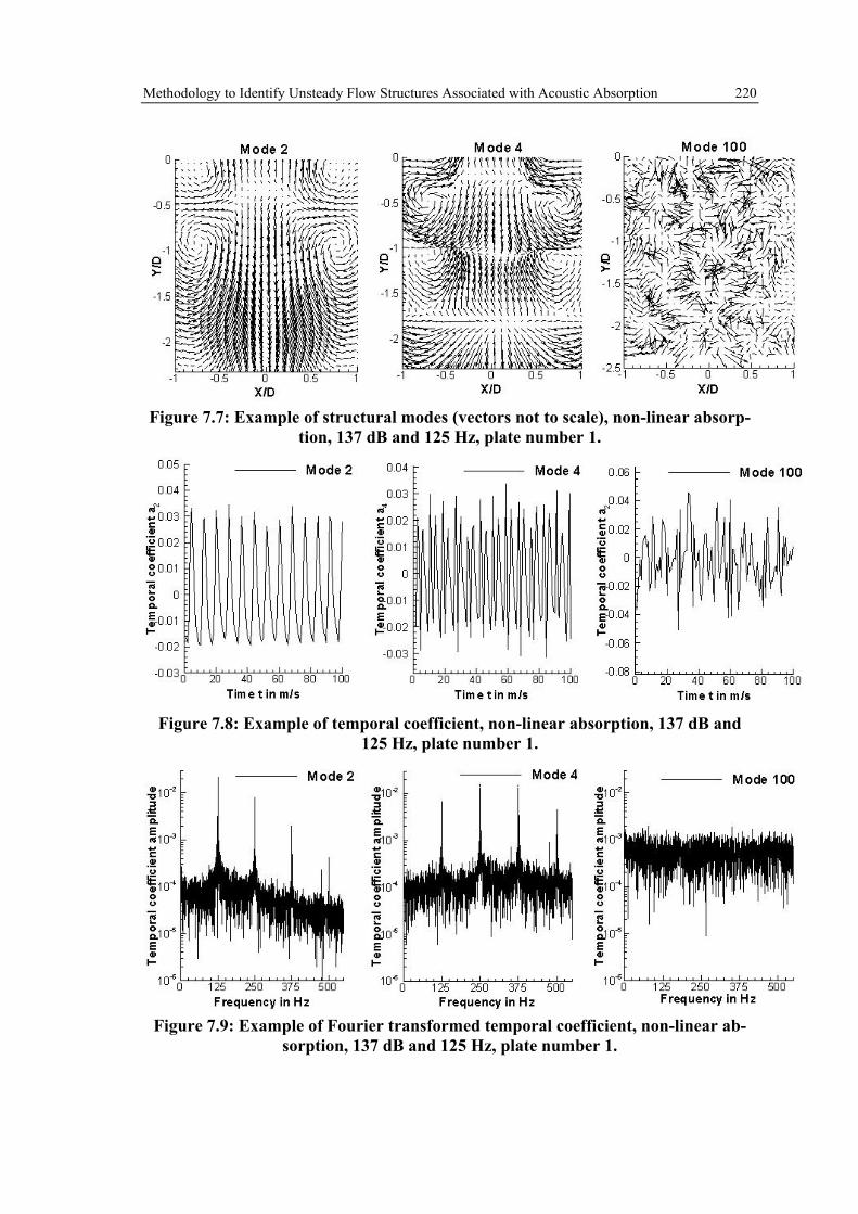
Methodology to Identify Unsteady Flow Structures Associated with Acoustic Absorption 220
Figure 7.7: Example of structural modes (vectors not to scale), non-linear absorp-
tion, 137 dB and 125 Hz, plate number 1.
Figure 7.8: Example of temporal coefficient, non-linear absorption, 137 dB and
125 Hz, plate number 1.
Figure 7.9: Example of Fourier transformed temporal coefficient, non-linear ab-
sorption, 137 dB and 125 Hz, plate number 1.
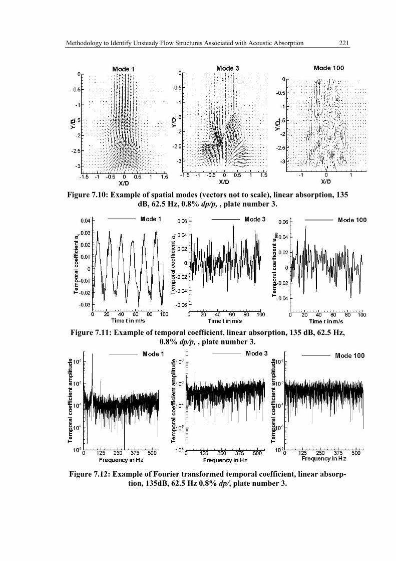
Methodology to Identify Unsteady Flow Structures Associated with Acoustic Absorption 221
Figure 7.10: Example of spatial modes (vectors not to scale), linear absorption, 135
dB, 62.5 Hz, 0.8% dp/p, , plate number 3.
Figure 7.11: Example of temporal coefficient, linear absorption, 135 dB, 62.5 Hz,
0.8% dp/p, , plate number 3.
Figure 7.12: Example of Fourier transformed temporal coefficient, linear absorp-
tion, 135dB, 62.5 Hz 0.8% dp/, plate number 3.

Methodology to Identify Unsteady Flow Structures Associated with Acoustic Absorption 222
0 100 200 300 400 500 600
Tem
pora
l coe
ffici
ent a
k
Frequency in Hz
10-6
10-1
10-5
10-4
10-3
10-2
∆f
averagedamplitude
Figure 7.13: Example of developed filter for temporal coefficient, Mode 2, 137 dB,
125 Hz, non-linear absorption regime, plate number 1.
0
20
40
60
80
100
120
140
0 20 40 60 80 100
Cum
ulat
ive
kine
tic e
nerg
y in
%
POD mode number
Cumulative kinetic energy
Filtered POD modes
Figure 7.14: Example of filtered POD modes in the non-linear absorption regime

Methodology to Identify Unsteady Flow Structures Associated with Acoustic Absorption 223
0
20
40
60
80
100
120
140
0 20 40 60 80 100
Cum
ulat
ive
kine
tic e
nerg
y in
%
POD mode number
Cumulative kinetic energy
Filtered POD modes
Figure 7.15: Example of filtered POD modes in the linear absorption regime
Figure 7.16: Position of calculated power spectral density, non-linear absorption.

Methodology to Identify Unsteady Flow Structures Associated with Acoustic Absorption 224
0 100 200 300 400 500 600
PSD
-v-
velo
city
com
pone
nt
Frequency in Hz
Total velocity fieldAcoustic velocity fieldTurbulent velocity field
102
103
104
101
100
10-1
10-2
Figure 7.17: Power spectral density of the v-velocity component on the jet centre-
line, x/D = 0 and y/D = -0.4
0 100 200 300 400 500 600
PSD
-v-
velo
city
com
pone
nt
Frequency in Hz
Total velocity fieldAcoustic velocity fieldTurbulent velocity field
102
103
104
101
100
10-1
10-2
Figure 7.18: Power spectral density of the v-velocity component in the shear layer
at x/D = 0.4 and y/D = -0.6

Methodology to Identify Unsteady Flow Structures Associated with Acoustic Absorption 225
Figure 7.19: Position of calculated power spectral density, linear absorption.
0 100 200 300 400 500 600
PSD
-v-
velo
city
com
pone
nt
Frequency in Hz
Total velocity fieldAcoustic velocity fieldTurbulent velocity field
102
103
104
101
100
10-1
10-2
Figure 7.20: Power spectral density of the v-velocity component on the jet centre-
line, linear absorption regime, x/D = 0 and y/D = -0.3

Methodology to Identify Unsteady Flow Structures Associated with Acoustic Absorption 226
0 100 200 300 400 500 600
PSD
-v-
velo
city
com
pone
nt
Frequency in Hz
Total velocity fieldAcoustic velocity fieldTurbulent velocity field
102
103
104
101
100
10-1
10-2
Figure 7.21: Power spectral density of the v-velocity component in the jet shear
layer, linear absorption regime, x/D = 0.3 and y/D = -0.8
POD Filtered periodic flow field Raw velocity field
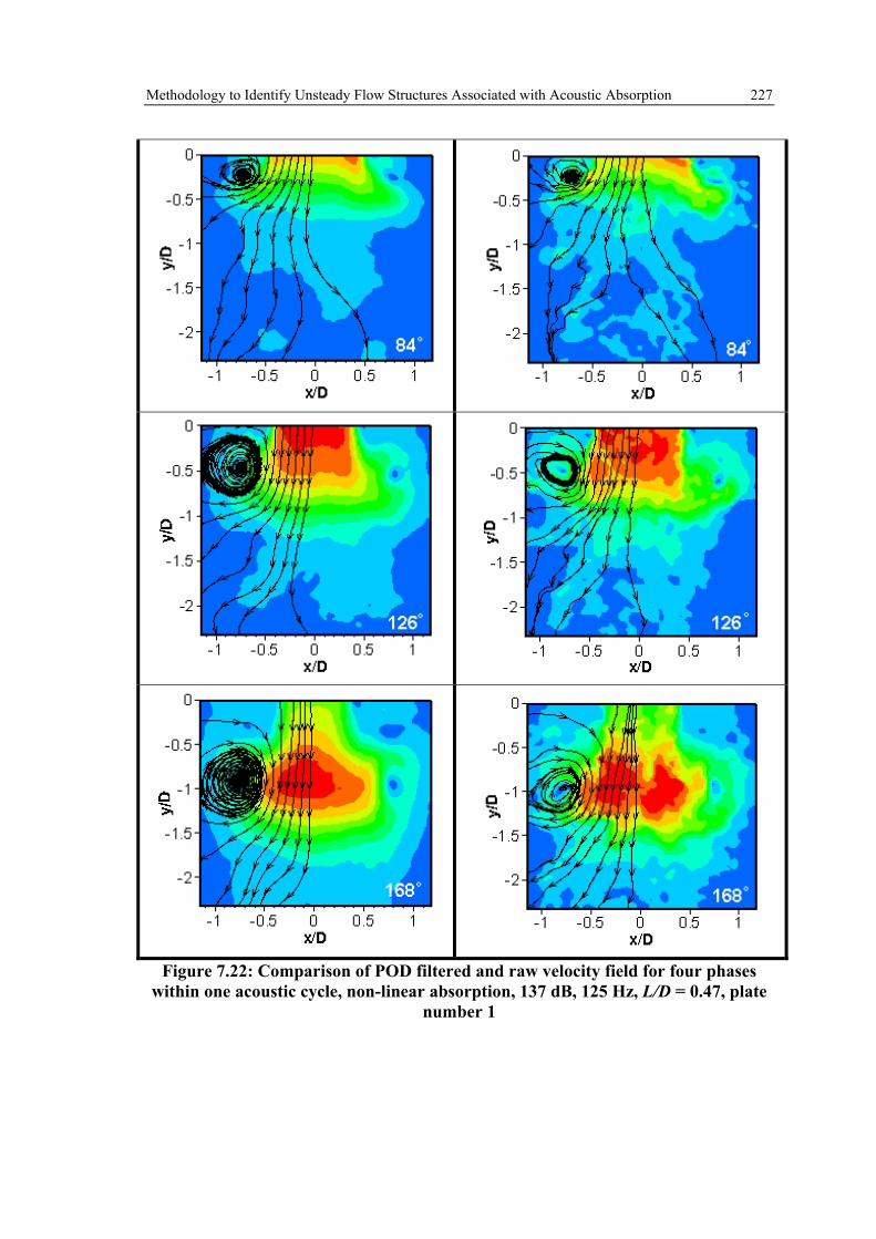
Methodology to Identify Unsteady Flow Structures Associated with Acoustic Absorption 227
Figure 7.22: Comparison of POD filtered and raw velocity field for four phases
within one acoustic cycle, non-linear absorption, 137 dB, 125 Hz, L/D = 0.47, plate number 1

Methodology to Identify Unsteady Flow Structures Associated with Acoustic Absorption 228
POD Filtered periodic flow field Raw velocity field
Figure 7.23: Comparison of POD filtered and raw velocity field for four different instantaneous flow fields within one acoustic cycle, linear absorption, 137 dB, 62.5
Hz, L/D = 0.5, plate number 3.

Methodology to Identify Unsteady Flow Structures Associated with Acoustic Absorption 229
0.0
0.2
0.4
0.6
0.8
125 130 135 140 145
Kin
etic
ene
rgy
flux
in J
/s
Excitation amplitude in dB
Acoustic measurementFiltered velocity fieldTotal velocity field
Non-linear absorption, Plate number 1.
0.00
0.02
0.04
0.06
0.08
0.10
0.0% 0.3% 0.6% 0.9%
Kin
etic
ene
rgy
flux
in J
/s
dp/p Linear absorption, Plate number 3.
Figure 7.24: Averaged kinetic energy flux per acoustic cycle compared to acoustic energy loss
Figure 7.25: Example of forced and unforced mean flow field, non-linear acoustic
absorption, L/D = 0.47, f = 125 Hz, plate number 1.

Methodology to Identify Unsteady Flow Structures Associated with Acoustic Absorption 230
r, x, uR
y, v
Control volume
Kinetic energy in control volume
( ) ( )( )∫ ∫ +=L R
dydrrtrvtruE0 0
22 ,,ρπ
r, x, uR
y, v
Circular planenormal to the
x,y - plane
Energy flux across exit surface
( ) ( ) ( )∫ +=R
drrtrvtrutrvE0
22 ),,(,ρπ
Figure 7.26: Schematic of control volume of kinetic energy calculation and control surface of kinetic energy flux calculation
0.0
0.1
0.2
0.3
0.4
0.5
0.6
0.7
0.8
130 132 134 136 138 140 142 144
Aver
aged
kin
etic
ene
rgy
flux
in J
/s
Excitation amplitude in dB
Acoustic energy loss
Kinetic energy flux unsteady jet
Max kinetic energy in control volume
Figure 7.27: Comparison between acoustic energy loss and kinetic energy con-
tained in the unsteady flow field

Methodology to Identify Unsteady Flow Structures Associated with Acoustic Absorption 231
-4.0
-3.0
-2.0
-1.0
0.0
1.0
2.0
3.0
4.0
0.0
0.2
0.4
0.6
0.8
1.0
1.2
0 0.2 0.4 0.6 0.8 1
v(t)/
Ubl
ow
E kin
(t)/E
kin,
max
t/T
Kinetic energy
Velocity
_
Figure 7.28: Comparison between acoustic energy loss and kinetic energy con-
tained in the unsteady flow field, 131 dB excitation
Figure 7.29: Vorticity contours at various time steps during change from in – to
outflow, downstream flow field.

Methodology to Identify Unsteady Flow Structures Associated with Acoustic Absorption 232
0
10
20
30
40
50
60
70
80
90
120 125 130 135 140 145 150
Phas
e an
ge in
deg
rees
Incident acoustic wave amplitude |p-| in dB^
Figure 7.30: Phase between pressure and velocity amplitude (acoustic impedance) for non-linear absorption measurement. Plate number 1, L/D =0.47.
-5.0
-4.0
-3.0
-2.0
-1.0
0.0
1.0
2.0
3.0
0.0 0.2 0.4 0.6 0.8 1.0
v(t)/
Ubl
ow
t/T
131 dB137 dB142 dB
_
Figure 7.31: Centreline velocity oscillation for phase averaged downstream flow
field, x/D = 0.0, y/D = -0.07, L/D = 0.5, plate number 1.

Methodology to Identify Unsteady Flow Structures Associated with Acoustic Absorption 233
Figure 7.32: Downstream velocity contour during flow direction sign change from
downstream to upstream flow direction. Non-linear forcing, L/D = 0.47, plate number 1.
Figure 7.33: Example of phase averaged centreline v-velocity oscillations at x/D = 0
and y/D = -0.07 for the acoustic related flow field, POD mode 1 and POD mode 1 without mean flow. L/D = 0.5 and L/D = 1, plate number 3 and 4, 62.5 Hz forcing.

Methodology to Identify Unsteady Flow Structures Associated with Acoustic Absorption 234
Figure 7.34: Example of phase averaged total velocity contours for the acoustic
related flow field. L/D = 0.5, plate number 3, 62.5 Hz forcing

Methodology to Identify Unsteady Flow Structures Associated with Acoustic Absorption 235
Figure 7.35: Example of phase averaged total velocity contours for the flow field of
POD mode 1 only. L/D = 0.5, plate number 3, 62.5 Hz forcing.
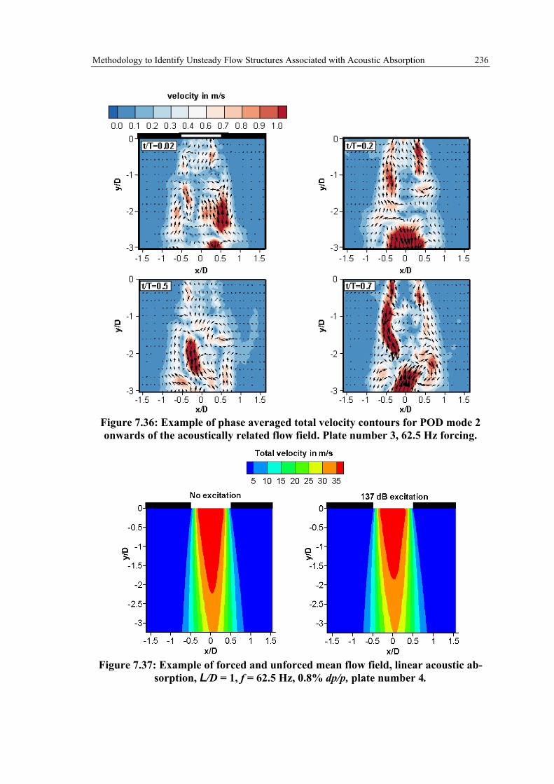
Methodology to Identify Unsteady Flow Structures Associated with Acoustic Absorption 236
Figure 7.36: Example of phase averaged total velocity contours for POD mode 2 onwards of the acoustically related flow field. Plate number 3, 62.5 Hz forcing.
Figure 7.37: Example of forced and unforced mean flow field, linear acoustic ab-
sorption, L/D = 1, f = 62.5 Hz, 0.8% dp/p, plate number 4.

Methodology to Identify Unsteady Flow Structures Associated with Acoustic Absorption 237
Cylindrical orifice L/D = 0.5 Conical orifice L/D = 2
0.1
0.2
0.3
0.4
0.5
0.6
120 130 140 150
Abso
rptio
n co
effic
ient
-∆
Excitation amplitude in dB
dp/p = 0.3%dp/p = 0.1%PIV data points
0.1
0.2
0.3
0.4
0.5
0.6
120 130 140 150Ab
sorp
tion
coef
ficie
nt -
∆
Excitation amplitude in dB
dp/p = 0.3%dp/p = 0.1%PIV data Points
Figure 7.38: Example of acoustic absorption coefficient and PIV data points for transition from linear to non-linear acoustic absorption, plate number 3 and 13.
Figure 7.39: Example of phase averaged normalised v-velocity and v-velocity spec-
trum of the acoustically related flow fields at x/D = 0 and y/D = -0.26. L/D = 0.5, dp/p = 0.1 and 0.3%, plate number 3, 62.5 Hz forcing.

Methodology to Identify Unsteady Flow Structures Associated with Acoustic Absorption 238
Figure 7.40: Example of phase averaged normalised v-velocity and v-velocity spec-trum of the acoustically related flow fields at x/D = 0 and y/D = -0.26. Conical aper-
ture, dp/p = 0.1 and 0.3%, plate number 13, 62.5 Hz forcing.
Figure 7.41: Example of phase averaged normalised total velocity contours acous-tically related flow field during linear acoustic absorption. L/D = 0.5, dp/p = 0.3%,
plate number 3.

Methodology to Identify Unsteady Flow Structures Associated with Acoustic Absorption 239
Figure 7.42: Example of phase averaged normalised total velocity contours acous-tically related flow field during transition to non-linear acoustic absorption. L/D =
0.5, dp/p = 0.1%, plate number 3.
Figure 7.43: Example of phase averaged normalised total velocity contours of
acoustically related flow field during transition to non-linear acoustic absorption. L/D = 2, dp/p = 0.1%, plate number 13.

Combustion System Passive Damper Design Considerations 240
8 Combustion System Passive Damper Design Considerations
Designing an efficient acoustic damper system to operate within a real engineering
environment such as a gas turbine engine is challenging. This is even more so if the
acoustic damper has to be located within the combustion chamber, when typically it is
directly coupled with the heat release region. This means that various other design
constraints must be considered such as (Rupp et. al. (2012)):
- The damper inner surface will be exposed to a relatively complex flow field. For
example, this could include an impinging swirling fuel injector flow or the passage of a
coolant film across the surface. The interaction of the swirling and cross flow
phenomena with the pulsatile flow field of the damper apertures could potentially
generate large scale structures within the unsteady jet shear layers (e.g. Lim et al
(2001)). As discussed in the previous sections (chapter 5 and 6), the current analytical
models within the linear and non-linear regime are not capturing well the influences of
large scale flow structures such as vortex rings. Thus, there could be large discrepancies
in the prediction of the acoustic damping performance due to the complex interaction
between the combustor flow field and the flow associated with acoustic damping.
- The perforated liner can form part of the combustion chamber wall. However, the
pressure drop across the flame tube is dictated by the fuel injector and the need to
generate sufficient turbulent mixing of the air and fuel passing through it. A perforated
liner exposed to this same pressure drop would result in a very high mean (bias)
velocity through the orifice which leads to reduced acoustic energy loss as discussed in
chapter 5 (see equation (5.26)). As a consequence an additional metering skin is
required to reduce the pressure drop and control the amount of bias flow through the
damper.
- The double skin damping system must be incorporated within a limited space
envelope. This is because the combustion system casing, defining the volume available
in the annulus surrounding the combustion chamber, has to be kept to a minimum

Combustion System Passive Damper Design Considerations 241
diameter to reduce the weight impact on the combustion system design for aero-engine
applications.
- The flame tube liner cooling requirements dictate a certain level of cooling flow, per
unit surface area, to maintain the structural integrity of the liner material. This means
the number and size of the orifices, within the perforated liner, must consider both
cooling and acoustic absorption requirements.
- The cooling design of such a damping system must also consider the potential for
hot gas ingestion into the passive damper geometry. Hence the mean pressure drop over
the final hot skin has to be carefully chosen. This is because the unsteady velocity
amplitudes, relative to the mean velocity, must be considered so as to avoid large
pressure amplitudes driving hot gas into the passive damper.
This chapter is concerned with the design of dampers for an aero-engine gas turbine
combustion system. Initially isothermal experiments in which a single sector of a gas
turbine aero-engine style combustor is simulated are described. A non-resonant liner
was incorporated in the test rig and its acoustic absorption characteristic has been
assessed experimentally. A simplified analytical model was developed based on the
findings described in Chapter 5 and validated against the experimental measurements.
In this way the observed acoustic performance can be related to the fundamental
processes generated by the incident acoustic waves. Furthermore the validated acoustic
model enables a prediction of the performance of a wide range of acoustic geometry, at
a variety of operating conditions, to be investigated. Moreover the model has also been
validated against acoustic absorption experiments using resonant acoustic liner concepts
to demonstrate the advantages of such damper technologies in the confined design space
of a gas turbine combustion chamber.
8.1 Analytical Model Development A simple one-dimensional analytical model was developed enabling the interpretation
of the experimental results as also introduced in Rupp et. al. (2012). The model is also
intended to be used as a rapid passive damping design tool to optimise acoustic
absorbers for gas turbine combustors. Moreover the performance of the Rayleigh
Conductivity modelling methods as described in chapter 5 can be further investigated

Combustion System Passive Damper Design Considerations 242
on representative multi-aperture acoustic damping systems. Figure 8.1 shows a
schematic of the underlying geometry simulated by the developed analytical model. The
model assumes that the acoustic wavelength is much greater than the liner length (i.e. a
‘long wavelength’ assumption) so that a uniform fluctuating pressure ( ( ) constyp ='0 ) is
imposed on the face of the damper.
This fluctuating pressure generates velocity perturbations leading to fluctuations in (i)
the mass flow entering ( inm ) and leaving ( outm ) the volume between the damping skins
and (ii) fluctuations in pressure inside the cavity ( '1p ). Hence the time dependent mass
flow variation inside the volume (V) between the skins is
''outin mm
dtd
Vdtdm
−==ρ .
( 8.1)
Assuming isentropic fluctuations ( ρργ '' =pp ) then
( ) '''
outin mmpp
Vi −=1
11 γ
ρR . ( 8.2)
where ( )tipp Rexpˆ' = , ( )timm Rexpˆ= etc. Note that it is assumed the gap between the
skins is not of sufficient size to result in the generation of mode shapes within the
damper cavity (i.e. uniform properties within the cavity). Hence it can be shown that:
[ ] [ ]112211
11111
DDoutin uAuAiV
pmm
iVp
p ˆˆˆ '' ρρR
γρR
γρ
−=−= . ( 8.3)
The area A is defined as the damper geometric hole area which is the sum of the
geometric area of each aperture, e.g. 211 RNA π= where N1 represents the amount of
apertures in the liner. Furthermore the parameters 1Du and 2Du are the unsteady
velocities associated with the 1st (damping) and 2nd (metering) skins. In the initial work
described in Rupp et. al. (2012) the model used to describe the velocity amplitudes
across the liner was based on the modified Howe model (as described in section 5.8)
using the compliance expression as defined in Eldredge and Dowling (2003). In this
work the modified Howe model was calibrated using the single aperture measurements
as, for example, shown in chapter 5 leading to good agreement with the experiments

Combustion System Passive Damper Design Considerations 243
shown in Rupp et. al. (2012). However, the dampers investigated in this study operate at
low Strouhal number (i.e. Strouhal numbers smaller than the Strouhal number of
maximum admittance). Section 5.8 highlighted the discrepancies of the Howe models in
this Strouhal number regime. In this region the change in aperture length-to-diameter
ratio and the associated change in the unsteady flow field were not reproduced by the
modified Howe model which can lead to significant errors in the prediction of absorbed
acoustic energy. As shown in section 5.9, the unsteady flow field, within the Strouhal
number regime considered here, is much more reliably represented by the momentum
balance introduced by Bellucci et. al. (2004). Therefore this approach has been
implemented in the current analytical model. Thus the velocity amplitudes in the plane
of the apertures can be calculated using the following two equations, one for each
damping skin, based on the described linear model in section 5.9:
0111111011 =++−+ DDDvis uUuppuLi ˆˆˆˆˆ , ρςρςRρ and ( 8.4)
022222122 =+++ DDvis uUupuLi ˆˆˆˆ , ρςρςRρ . ( 8.5)
Hence the unsteady velocities are defined as:
1111
011 LiU
ppu
visDD Rρρςρς ++
−=
,
ˆˆˆ and
( 8.6)
2222
12 LiU
pu
visDD Rρρςρς ++
−=
,
ˆˆ .
( 8.7)
It can be seen that the unsteady velocity across the apertures in the damping skin is
affected by four components:
(i) the unsteady pressure difference between the incident amplitude ( 0p ) and the
pressure amplitude inside the cavity ( 1p ).
(ii) the resistance of the aperture which is a function of the mean jet flow and its loss
coefficient 11 DUρζ
(iii) the reactance due to the acceleration forces onto the mass of the fluid within the
aperture 1LρR

Combustion System Passive Damper Design Considerations 244
(iv) the viscosity due to the boundary layer within the aperture 1,visρζ (as described
in equation (5.34)), which is an additional contribution to the aperture
resistance as well as the reactance.
The same applies to the metering skin aperture with the exception that the upstream
pressure amplitude is assumed to be negligible as the liner is plenum fed. As described
in chapter 5.9 the loss coefficients 1ζ and 2ζ can be approximated using the mean flow
discharge coefficient of the damping and metering skins. The discharge coefficients for
the perforated liner geometries have been measured on the facility described in
appendix B and used in the model to calculate the acoustic absorption at the relevant
liner pressure drop and Reynolds number representative of the operating conditions
during the acoustic experiments. The measured discharge coefficients were used as in
equation (5.35) to calculate the loss coefficient for the resistance of the perforated
plates. Moreover the length correction for the effective length of each perforated plate
was estimated using the single orifice geometries defined in Table 5.1.
Equations ( 8.3), ( 8.6) and ( 8.7) form a linear equation system which can be solved
analytically. According to Bellucci et. al. (2004) the absorbed acoustic energy can be
calculated as:
( ) 10121 ApuL ˆˆRe *=Π ,
( 8.8)
or in accordance with Howe (1979b) or Luong et. al. (2005):
2222
1112 N
RpN
Rpp uduL ρR
δρR
δ ˆˆˆ +−=Π . ( 8.9)
Both acoustic energy expressions have been used in this work and lead to the same
result and therefore include the acoustic energy being absorbed by the damping and
metering skins. It can be seen that the acoustic energy loss calculated from equation
( 8.8) is a function of the unsteady velocity amplitude which is expressed in equation
( 8.9) by the unsteady pressure difference and the admittance for each liner. Hence the
acoustic absorption can be increased by increasing the unsteady velocity amplitudes
across the apertures.

Combustion System Passive Damper Design Considerations 245
Finally the acoustic energy loss is normalised with the excitation pressure amplitude
( 0p ) as proposed in Rupp et. al. (2010):
20p
LP
ˆ
Π=Π .
( 8.10)
This normalisation makes the results independent of the applied pressure amplitude
within the linear acoustic absorption regime. Moreover the incident pressure amplitude
is used as an inlet condition into the model.
8.2 Non-Resonant Passive Damper As described in Rupp et. al. (2012) most experimental and theoretical investigations
have considered the performance of perforated liners within a simple 1D duct type flow
or impedance tube, e.g. Eldredge and Dowling (2003), Hughes and Dowling (1990),
Lahiri et. al. (2011). However, considered here is the application of a perforated liner to
aero style gas turbine combustion systems. This study has been undertaken on the
experimental facility described in chapter 3.3.2. In this case a passive damper which
consists of a porous liner and metering skin can be incorporated into the flame tube
liner. Plane axial acoustic waves are generated by loudspeakers and pass into the
combustor test section. Based on the magnitude of the incident and reflected waves an
assessment can be made of the acoustic energy being absorbed in this relatively
complex environment.
8.2.1 Experimental Results The experimental results and discussions in this section can also be found in Rupp et.
al. (2012). As already discussed the flow field in the vicinity of the perforated liner in
the test section will be affected by the swirling flow field of a fuel spray nozzle which
was also incorporated on the test rig. The fuel injector geometry was representative of a
lean burn combustion technology fuel spray nozzle. However in this case the injector
was only used to provide a representative swirling flow field impinging onto the
perforated liner. The burner was provided by the industrial partner in this project and its
geometry remains confidential but is representative of the geometry likely to be used
with future low emissions aero-engines. The mean pressure drop across the passive

Combustion System Passive Damper Design Considerations 246
damper, as well as the fuel injector, was set to 3% which is also thought typical of gas
turbine combustion system pressure drops.
The mean static pressure distribution measured on the face of the damping skin is
presented (Figure 8.2). The contours show the static pressure difference between the
actual static pressure and the reference pressure in the centre of the perforated liner, i.e.
x/WD = 0.5 and y/LD = 0.6. This was non-dimensionalised using the spatially averaged
mean pressure difference across the damping skin. Note the highly non-uniform
distribution being measured on the face of the damper. A high static pressure is observed
where the efflux from the injector impinges onto the passive damper (and y/LD < 0.4),
this pressure being greater than the design pressure drop across the damping skin. In
other words at this location the pressure on the damper face, inside the flame tube, is
greater than the pressure within the cavity between the porous liners. This must give rise
to some concern regarding the ingestion of hot gas into the cavity between the damping
and metering skins. As fluid accelerates away from the impingement point the static
pressure reduces so increasing the pressure drop across the damping skin. On a spatially
averaged basis the damping skin is designed to operate in a linear absorption regime
such that any fluctuations in velocity associated with the acoustic pressure oscillations
is less than the mean velocity through the orifices. However, on a local basis the
measurements suggest that, potentially, this may not be the case.
With the loudspeakers activated a typical mode shape is presented (Figure 8.3), this
being normalised by the maximum pressure amplitude. As to be expected in all cases a
pressure anti-node is located close to the downstream face of the injector. Thus the
proximity of the damper to the fuel injector means that the damper is also exposed to a
region of high pressure fluctuations, although these fluctuations will reduce towards the
damper trailing edge. This variation is a function of the acoustic wavelength relative to
the damper length. From data such as this the magnitude of the acoustic waves
travelling towards, and away from, the test section can be calculated. In terms of an
energy budget the acoustic energy travelling towards the test section can either (i) pass
through the fuel injector, (ii) be absorbed by the damper, or (iii) be reflected back down
the duct. Usually the reflection coefficient is defined as the ratio of the reflected and
incident pressure amplitude. However, for convenience, in this case the reflection

Combustion System Passive Damper Design Considerations 247
coefficient was defined as the ratio between the incidence and reflected acoustic energy
i.e.
2
22
i
rC
B
BR
ˆ
ˆ= . ( 8.11)
Initially the reflection coefficient was measured over a range of frequencies for the
case where the damper was replaced by a solid surface (Figure 8.4). In this case the
difference between the incident and reflected acoustic energy reflects that portion of the
acoustic energy that is being transmitted through the fuel injector. For example, at 300
Hz the results indicate approximately 35% of the incident energy is reflected back down
the duct, with the remaining energy (65%) exiting the test section through the fuel
injector. In addition, results are also presented with the passive damper present in which
the gap between the two skins was set to its datum value (S/H = 0.125). Note that other
tests performed at smaller gaps also indicated a similar reflection coefficient. The
reduction in reflected energy is associated with the inclusion of the passive damper
assembly and the absorption of acoustic energy by the damper. However, additional
tests were also performed in which the damping skin was removed and only the
metering skin was present (placed flush with the inside surface of the duct). Note the
similarity in the reflection coefficient over the range of frequencies tested. This suggests
that for this datum configuration the acoustic energy absorption was associated with the
metering skin, with no acoustic energy being absorbed by the damping skin. However,
further measurements were undertaken with the passive damper in place but where the
gap between the two liners was increased, in various increments, from 0.125 ≤ S/H ≤
1.46 (Figure 8.5). It can be seen that with an increasing gap the amount of reflected
energy decreases until, at the larger separations, virtually no acoustic energy is being
reflected back from the test section. In other words for these configurations the results
suggest a relatively large amount of acoustic energy is being absorbed. This behaviour
is clearly an important aspect relating to the design of an efficient passive damping
system within a gas turbine space envelope. Therefore the aforementioned acoustic
absorption model (section 8.1) was used to investigate the observed characteristic

Combustion System Passive Damper Design Considerations 248
relating to the reduction of increasing acoustic absorption with increasing damper
volume.
8.2.2 Analytical Model Validation Initially the model introduced in the previous section can be validated against the
experimental results in a similar way as described in Rupp et. al. (2012). Due to the
transmission of acoustic energy introduced by the fuel injector it is not possible to
directly compare the loss of acoustic energy between the experiment and the model
previously presented (i.e. the model only captures the loss associated with the passive
damping system and not the acoustic energy transmitted through the fuel injector).
Therefore the validation of the model is split into two sections. Initially the acoustic
energy loss calculated by the model will be compared to absorption measurements
conducted without the presence of the fuel injector. Afterwards the model is compared
to the pressure amplitude measurements in the presence of the fuel injector flow field.
The discharge coefficients used within the acoustic model for the damping skin and
metering skin as well as the length corrections are defined in Table 8.1. In this case the
mean flow discharge coefficients were measured using the test specimen and the
plenum fed arrangement described in appendix B. Moreover the length corrections were
estimated from the geometry used in Table 5.1.
L/D CD Length correction (Table 5.1)
Damping skin 2.86 0.88 1.35 (L/D = 3)
Metering skin 2 0.87 1.06 (L/D = 1.98) Table 8.1 Measured discharge coefficient and used loss coefficient in analytical
model
8.2.2.1 Acoustic Energy Absorption In this case the fuel injector is removed and replaced by a blanking plate. As the
upstream boundary condition in the test rig is now a closed end it can be assumed that
the difference between incident and reflected energy is only associated with the energy
absorbed by the passive damping system. All the experimental data compared to the

Combustion System Passive Damper Design Considerations 249
modelling data in this section (Figure 8.7) has been conducted with a closed wall
termination instead of the fuel injector.
For this configuration three test cases have been used (S/H = 0.125, 0.33 and 1.56 at a
∆p/p of 3% across the two perforated skins). The acoustic energy loss has been
calculated from the experiments using the difference in acoustic energy flux travelling
towards and away from the test section (as defined in equations (5.1) to (5.3)). As
already discussed the analytical model relies on the long wavelength assumption. At
relatively low frequencies the assumption of a constant pressure fluctuation across the
face of the damper will be valid but this may not be the case at higher frequencies.
Moreover the amplitude on the face of the damper, which is used to normalise the
acoustic loss, could be overestimated due to the appearance of the acoustic mode shape
along the face of the damper. With this in mind Figure 8.6 shows the measured mode
shapes for 250, 300 and 350 Hz (note that the amplitudes have been normalised with the
maximum pressure amplitude).
To reduce the source of error, due to the changing pressure amplitude along the
damper surface, the measured mode shapes were used as an input to the model. The
associated velocity fluctuations described in equation ( 8.6) for the metering and
damping skins have been divided into n sections with a damper length of dL = L/n. In
this way the input excitation amplitude ( )yp0ˆ has been set according to the mode shape
amplitudes along the y-axis, i. e.:
( )
( )
( ).
ˆˆˆ
ˆˆˆ
ˆˆˆ
,
,
,
1111
011
1111
20112
1111
10111
LiUypp
u
LiUypp
u
LiUypp
u
visD
nnD
visDD
visDD
Rρρςρς
Rρρςρς
Rρρςρς
++−
=
++−
=
++−
=
The linear equation system was then solved and the energy loss of each section along
the damping skin surface was accumulated to give the total energy loss. Thus acoustic
energy loss has been normalised according to equation ( 8.10) using the spatially
averaged pressure amplitude on the face of the damper inside the main duct.

Combustion System Passive Damper Design Considerations 250
Figure 8.7 shows the comparison of the experimental data to the mode shape
corrected analytical absorption model. It can be seen that the model shows very good
agreement throughout the frequency range. However to reduce any ambiguity due to the
normalisation of the acoustic loss Figure 8.8 compares the actual measured acoustic loss
with the loss calculated by the model using the mode shape pressure amplitude as an
input. It can be seen that there is excellent agreement between the model and the
measurement. It should be noted that when using the model for predicting damper
performance the measured mode shape is not known a priori. However this is deemed
acceptable within a preliminary design assessment (i) enabling the relative performance
of different damping configurations to be assessed and (ii) identifying the main factors
controlling the amount of acoustic absorption.
Another interesting aspect is the application of such an analytical model to annular
gas turbine combustor geometries. In this case the pressure excitation can be caused by
a circumferential wave travelling through the combustor annulus geometry. The
developed analytical model would be valid for a circumferential moving pressure wave
where the wavelength in the circumferential direction is much larger than the width of
the damper in circumferential direction. However, for more accurate calculations the
tool should be incorporated in acoustic network models simulating the actual pressure
mode shapes. In this way the effect of the acoustic damper on the combustor stability
can be assessed.
8.2.2.2 Damper Cavity Pressure Amplitude Assessment For the experimental data in this section the fuel injector was installed onto the test
rig. Hence no direct comparison of the acoustic energy loss due to the damper is
possible. However, as suggested by equations ( 8.6), ( 8.7) and ( 8.9) the unsteady
pressure drop across the damping and metering skins has a significant effect on the
amount of acoustic energy being absorbed. Hence some further validation of the model
was conducted comparing the ratio of pressure amplitudes inside the cavity, 1p (i.e.
between the damping and metering skins), with those within the test section, op (i.e.
incident onto the damping skin). Again in this case the pressure mode shape along the
face of the damper has been averaged over the axial length of the damper to estimate the

Combustion System Passive Damper Design Considerations 251
incident pressure amplitude op . Space constraints meant that experimentally the cavity
pressure amplitude could only be measured for liner separations greater than 0.33.
However some example results are presented (Figure 8.9) for which measurements were
available.
It can be seen that the model is able to capture the pressure ratio indicated by the
experimental data. This includes the reduction in the oscillating cavity pressure
amplitude, relative to the pressure incident onto the damping surface, with increasing
liner separation. Moreover Figure 8.10 shows the phase difference between the cavity
pressure oscillation and the incidental pressure oscillation as a comparison between the
measured data and the prediction by the model. In this case the phase of the incidental
pressure wave was averaged along the damper surface. As the cavity measurement is a
point measurement it was assumed that there is no significant phase change within the
cavity between the damping and the metering skin. It can be seen that the model is
agreeing very well with measured phase difference across the damping skin. Moreover
the trend of increasing phase difference with increasing cavity volume is also captured
well by the model. Overall it can be seen that the model is capable of predicting the
acoustic characteristics of the double liner system despite the complex mean flow
condition the damping skin is operating in. As already described in section 5.9 the
model takes no account of the complexity of the flow field and simulates a pulsatile
flow field based on a constant loss coefficient and length correction. Hence the good
agreement between the experiment and the model suggests that the swirling flows and
cross-flows along the damper surface have no significant effect on the overall damper
performance. Moreover this data indicates that overall the absorption is linear on the
face of the damper (although locally this may not be the case due to the pressure drop
distribution for the cases with fuel injector). Due to the very good agreement between
the model and the experimental results the model can now be used to further understand
the absorption behaviour of the investigated passive damper geometry.
8.2.3 Damper Performance Assessment As described in Rupp et. al. (2012) both the experimental measurements and
analytical model have been used to relate the observed absorption characteristics with

Combustion System Passive Damper Design Considerations 252
the unsteady flow field generated by the incident acoustic waves. The previous section
has shown the model is most accurate if a representative input mode shape profile is
used into the model. Hence the experimental mode shape measurement from the S/H =
1.56 test case has been used as input to the model. However in this case only the profile
of the mode shape along the y-axis is important, not the actual amplitude of the mode
shape. Hence calculations from other test cases do generate identical results for
equivalent frequencies.
For aero-type applications there is a desire to minimise the space occupied by the
damping system so resulting in a relatively small separation, or volume (V), between the
metering and damping skins. However, this small volume means that the pressure inside
the cavity is sensitive to any changes in mass flow. The incident acoustic pressure
fluctuation will therefore cause a change in mass flow, through the damping skin, which
quickly leads to a change in the cavity pressure (i.e. due to the small volume). In reality
this means that at small volumes the unsteady cavity pressure approximately equals the
unsteady incident pressure. Thus the unsteady pressure drop across the damping skin is
minimal. This is suggested both by the experiment data already presented (Figure 8.4
and Figure 8.5), and also the cavity pressures generated by the analytical model that
have been plotted for an excitation frequency of 250 Hz (Figure 8.11). The experimental
data measured in the presence of the fuel injector flow field was also added into Figure
8.11 for comparison. Moreover the phase between the cavity pressure and the excitation
pressure in Figure 8.12 shows that the fluctuations for small volumes occur in phase i.e.
as the incident pressure increases so does the cavity pressure at virtually the same
instant in time. Furthermore it can be seen that the analytical model is agreeing very
well with the measured phase even when the fuel injector flow field is present in the
experiment.
As a consequence at small cavity gaps nearly the entire unsteady pressure drop occurs
across the metering skin. This explains why there was little difference in the reflection
coefficient between tests undertaken with the single (metering) skin and with the
damper present when the cavity gap was less than S/H = 0.125. The metering skin is
designed with a high mean pressure drop and therefore the acoustic absorption
generated by the metering liner is relatively small. As the gap between the skins within

Combustion System Passive Damper Design Considerations 253
the passive damper increases, however, so the volume will tend towards a plenum. In
this case fluctuations in mass flow through the damping skin, due to the incident
unsteady pressure, will have a limited effect on the pressure within the damper cavity
(Figure 8.11). Consequently large unsteady pressure fluctuations and mass flow
variations are generated across the damping skin enabling a significant amount of
acoustic energy to be absorbed (Figure 8.5). This behaviour is also illustrated in Figure
8.13 where the predicted unsteady velocities (normalised with the mean velocities
across the damping and metering skins) are shown for a perturbation at 250 Hz. The
significant increase in the unsteady damping skin velocity with increasing liner
separation can be seen. In contrast at small volumes the unsteady damping skin velocity
is small and of the order of the metering skin velocity amplitudes. However in this case
the unsteady pressure drop across the damping skin is reduced which leads to a much
reduced acoustic energy loss as described in equation ( 8.9) and the majority of the
damping is caused by the metering skin. Even though the unsteady pressure drop across
the metering skin is increased for the small cavity volumes the large mean pressure drop
results in much smaller Strouhal numbers. Hence the admittance, which is also a
measure of the acoustic energy loss as indicated in equation ( 8.9), is much smaller for
the metering skin than for the damping skin (Figure 8.14). Thus the acoustic energy loss
is reduced for the metering skin despite the increased unsteady pressure difference.
8.2.4 Damper Optimisation In addition to understanding the unsteady flow field and the absorption characteristics
the simplified model can be used to explore the impact and trade-off between various
changes to the damper geometry in the same way as described in Rupp et. al. (2012). In
equations ( 8.8) and ( 8.9) it was shown that the pressure amplitude is proportional to the
unsteady velocity amplitude and the unsteady pressure drop. Previously section 5.7
showed that the maximum acoustic energy loss within the quasi-steady regime (low
Strouhal number) is proportional to the unsteady pressure difference and the ratio of
mean mass flow through the porosity and the mean pressure drop (equation 5.25)
.ˆˆ~p
mpp usds
QSL ∆
−Π2 ( 8.12)

Combustion System Passive Damper Design Considerations 254
The damper within the gas turbine combustion system has to operate within a given air
mass flow budget. Hence one way of optimising a damper is to reduce the mean
pressure drop for a given mean air mass flow by using a second liner (i.e. metering
skin). However as shown in the previous section reducing the mean pressure drop
across the damping skin might not be beneficial for the given space envelope and the
associated unsteady pressure difference which is also affecting the acoustic energy loss
(equation ( 8.9) and ( 8.12)). Hence the model is used to understand the optimum mean
pressure drop for a given cavity volume size. For example the amount of energy
absorbed, as indicated by the model, is presented for three different cavity separations
and for various combinations of metering skin and damping skin porosity. These
changes in porosity were achieved by varying the number of orifices within each skin.
The total pressure drop across the passive damper system was kept constant as well as
the mass flow through the damper.
Figure 8.15 presents the normalised acoustic loss with respect to a change in the mean
pressure drop across the damping skin. The occurrence of the acoustic loss maxima can
be explained by considering the acoustic loss defined by equation ( 8.9) as well as the
velocity amplitude equations ( 8.6) and ( 8.7). The acoustic energy loss is a function of
the unsteady pressure difference across the aperture and the admittance of the apertures.
Moreover equations ( 8.6) and ( 8.7) show that the velocity amplitudes are calculated
using the loss coefficients, mean velocity, length corrections and the unsteady pressure
drop. Hence changes in mean pressure drop will also result in changes in mean velocity.
If the length-to-diameter ratio is constant it can be assumed that the discharge
coefficient and thus the loss coefficient remain constant. Hence one strategy to increase
the absorption of a passive damper is to reduce the mean velocity, by reducing the mean
pressure drop. This will lead to an increase in velocity amplitude and therefore to an
increase in admittance for the apertures as explained in section 5.3. However as Figure
8.16 shows the cavity unsteady pressure ratio, for a given volume, increases with
decreasing mean pressure drop i.e. the cavity becomes more sensitive to mass flow
fluctuations and so the unsteady pressure drop across the damping skin decreases with a
decreasing mean pressure drop. Hence the possible increase in velocity amplitude, and
therefore the acoustic absorption, is also accompanied by a reduction in the unsteady

Combustion System Passive Damper Design Considerations 255
pressure drop. Consequently there is an optimum mean pressure drop across the
damping skin i.e. where the acoustic absorption is at its maximum for a given cavity
volume.
It can be seen from Figure 8.15 that the volume effect is much larger than the pressure
drop reduction. Hence the design of non-resonant acoustic dampers should aim at
maximising the available volume. As equations ( 8.8) and ( 8.9) show the actual area of
the damper (or amount of apertures within the damper) also affects the acoustic
absorption performance. However this parameter is set by the available air mass flow
budget. Hence the optimisation of a non-resonating damper can only aim on
optimisation of the porosities between the metering and damping skin such that the
unsteady pressure difference across the damping skin apertures is maximised. This
needs to be in conjunction with the necessary cooling requirements of the combustor
wall.
8.2.5 Impedance Methodology As already discussed in the previous section it is not straightforward to compare the
analytical modelling data to the measured data if the fuel injector is also present in the
experiment. In this case some of the energy is also transmitted through the fuel injector
or even dissipated by the fuel injector. Hence the measured reflection coefficient is
representative of the total system, i.e. fuel injector and acoustic damper. Therefore the
model also needs to consider the superposition of the acoustic characteristic of the fuel
injector (this being more representative of an engine configuration). Hence an approach
as described by Kinsler et. al. (1999) was implemented which enables the superposition
of impedances of the considered acoustic elements. This process is shown schematically
in Figure 8.17, and as previously discussed, assumes that the acoustic wavelength is
much longer compared to the length of the damper or size of the fuel injector. In this
case the test section is split into an acoustic system of three impedances: the damper
impedance ZD, the fuel injector impedance Zinj and the total impedance of the system
Ztot. In accordance with Kinsler et. al. (1999) this system of impedances has been split
into three acoustic branches joined together at the plane y/LD = 0. The plane at y/LD = 0
was chosen just downstream of the fuel injector. Hence as a first approximation the
assumption was made that the change in pressure amplitude along the damper is

Combustion System Passive Damper Design Considerations 256
negligible, i.e. ( ) 0=∂∂ DLyp . However this approach can be included within a
network model in the future which should take the mode shape along the damper
surface into account.
Mathematically the acoustic system can be described using impedances considering
the volume velocity (e.g. Kinsler et. al. (1999) or Lucas et. al. (1997))
( ) ( )( ) tottot
tot AxuxpxZ
000
==
==ˆ
ˆ,
( 8.13)
where Atot represents the cross-sectional area of the duct to which the fuel injector and
damper are connected. Applying continuity of mass across the boundaries of the
acoustic branches and assuming that all acoustic elements are exposed to the same
pressure amplitudes the total acoustic impedance can be described as
injinjDDtottot Aup
Aup
Aup
ˆˆ
ˆˆ
ˆˆ
+= . ( 8.14)
Hence the total impedance can be calculated as the sum of the reciprocal of the acoustic
component impedances
injDtot ZZZ111
+= . ( 8.15)
The acoustic impedance of the non-resonant acoustic damper is calculated using the
described analytical model. A representative pressure mode shape is used as input to the
model and the impedance is averaged along the face of the damper. This averaged
impedance is then used as the damper impedance in equation ( 8.15).
The remaining unknown is the fuel injector impedance. In this case the fuel injector
impedance was measured by blanking the damper section off with a rigid wall, with the
fuel injector upstream side being open to atmosphere (i.e. plenum fed). For this
configuration the acoustic impedance could be measured using the two microphone
method and a mean pressure drop across the fuel injector of 3%. The setup was not
optimised for an impedance measurement as for example explained in section 5.4.
Hence reference data was also used relating to the same injector in a similar plenum fed
arrangement forced by plane axial pressure waves (but over a wider frequency
Combustion System Passive Damper Design Considerations 257
bandwidth) conducted by Peacock (2011). The measured resistance and reactance of the
fuel injector is shown in Figure 8.18. Note that the impedances shown in this figure do
show the impedance based on the velocity amplitude, i.e. upZ ˆˆ= . For the purpose of
this work the measured fuel injector impedance could be matched using the momentum
balance as used in section 5.9 to calculate the impedance of the investigated orifice
geometry. In this case the assumption was made that the resistance of the injector
remains constant across the investigated frequencies with no viscosity effects being
considered. The fit to the experimental data obtained by changing the loss coefficient
and the acoustic length of the fuel injector is also shown in Figure 8.18. It should be
noted this is not suggested that this is the correct model to use, but for the purpose of
this work it was sufficient to get a reasonable representation of the fuel injector
boundary condition. The increase in resistance from 250 Hz and 350 Hz could be partly
due to real behaviour of the fuel injector or due to experimental inaccuracies. The only
frequency dependent change to the resistance on the basis of the used model from
section 5.9 would be the influence of viscosity. However this increase is too sharp to be
reproduced by the model. Nevertheless the fuel injector swirling flow field is complex
and flow instabilities in the swirling shear layers could also cause changes to the
resistance of the fuel injector. Similar behaviour was found for jet flow instabilities for
circular orifice plates in section 5.9. The fuel injector acoustic behaviour was not part of
this work and it is suggested that future projects could provide a better representation of
the acoustic characteristic of the injector. Ultimately this would increase the accuracy of
acoustic network models for combustion instabilities. Nevertheless the estimated
resistance and reactance was used to represent the fuel injector impedance in equation
( 8.14) to a first approximation.
The calculated total impedance from equation ( 8.14) was then used to estimate the
reflection coefficient as defined for example by Bellucci et. al. (2004):
cZcZ
Rtot
totC ρ
ρ−+
= . ( 8.16)
Hence the total system reflection coefficient estimated by the model with the help of
equations ( 8.14) and ( 8.15) has been compared with the measured reflection coefficient
for the total system of fuel injector and acoustic damper (Figure 8.19). It can be seen

Combustion System Passive Damper Design Considerations 258
that the calculated reflection coefficient agrees reasonably well with the measured
reflection coefficient. The previous two sections have shown the analytical damper
model agrees well with the measured acoustic losses and so any discrepancies in the
total system loss are most likely due to inaccuracies of the fuel injector impedance
measurements. To emphasise this source of error in the method a variation on the fuel
injector resistance and reactance is also presented. Figure 8.20 shows the measured fuel
injector impedance in comparison to a modelling match with increased resistance and
reactance. This has then been used to predict the total system reflection coefficient for
the example test case of S/H = 0.74 (Figure 8.21). It can be seen that the calculated
reflection coefficient is much increased compared to the previous solution with a
reduced resistance. This supports the suggestion that the fuel injector impedance is the
greatest source of error within the prediction and has also the largest effect upon the
total system reflection coefficient.
However the used method of reproducing rather complex multi-impedance system
experiments seems to be valid due to the generally good agreement between the model
and experiment. This can be used to validate elements of the acoustic network models
for multi-acoustic element experiments. As long as the system impedances, i.e. fuel
injector, tiles, dampers, are known the experimental data can be either split into single
element impedances or models of total systems can be reproduced. This enables the
acoustic assessment of complex acoustic systems (such as gas turbine combustion
systems).
8.3 Resonating Linear Acoustic Dampers One of the outcomes of the previous section was that the complex fuel injector flow
field has no significant effect upon the performance of the acoustic damper. Therefore
the acoustic damper geometries can be optimised on a simple test rig without the
influence of a fuel injector. Hence the experimental facility described in section 3.3.1
has been used to assess various acoustic damper designs as described in appendix A.3.
The previous section introduced a perforated liner system aimed at absorbing acoustic
energy within a gas turbine combustion system environment. In this case the cavity
between the damping skin and the metering skin was not resonating and it was shown
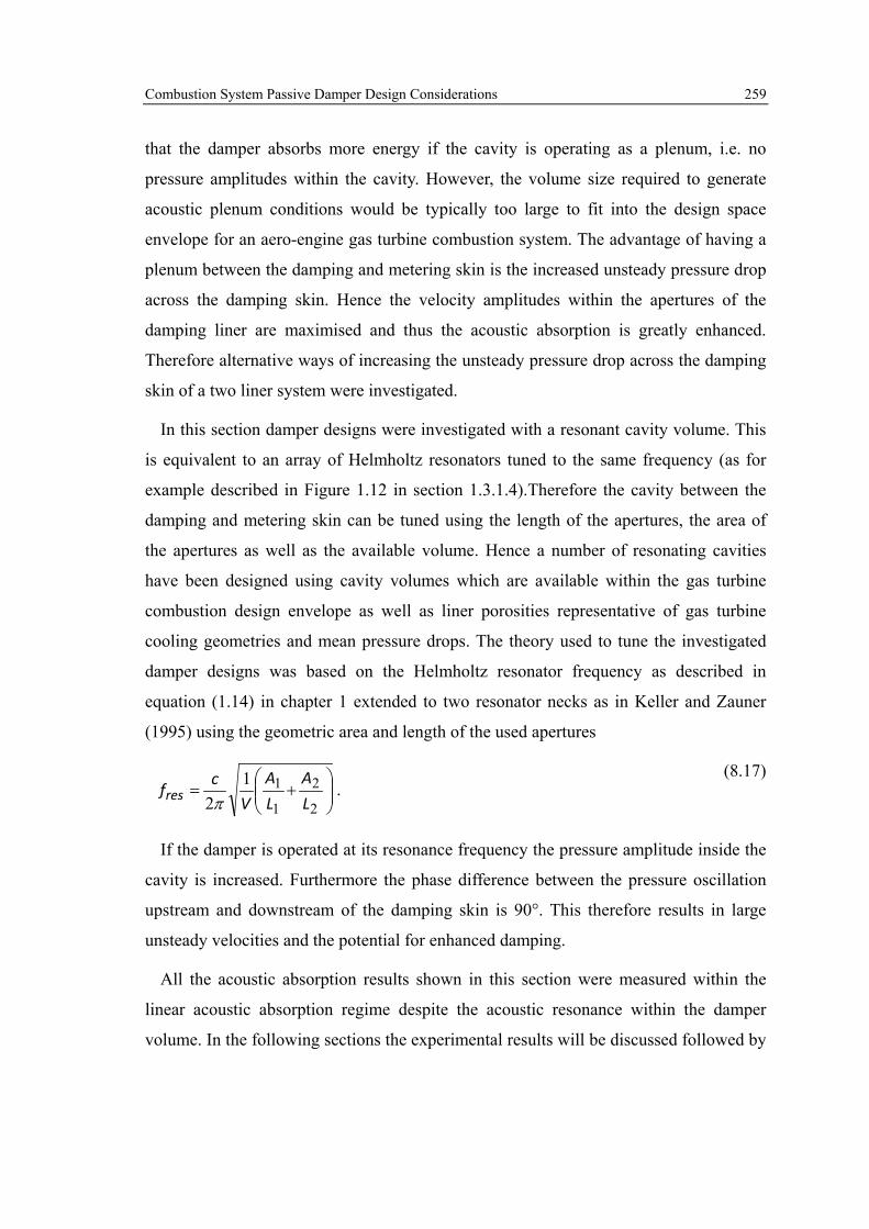
Combustion System Passive Damper Design Considerations 259
that the damper absorbs more energy if the cavity is operating as a plenum, i.e. no
pressure amplitudes within the cavity. However, the volume size required to generate
acoustic plenum conditions would be typically too large to fit into the design space
envelope for an aero-engine gas turbine combustion system. The advantage of having a
plenum between the damping and metering skin is the increased unsteady pressure drop
across the damping skin. Hence the velocity amplitudes within the apertures of the
damping liner are maximised and thus the acoustic absorption is greatly enhanced.
Therefore alternative ways of increasing the unsteady pressure drop across the damping
skin of a two liner system were investigated.
In this section damper designs were investigated with a resonant cavity volume. This
is equivalent to an array of Helmholtz resonators tuned to the same frequency (as for
example described in Figure 1.12 in section 1.3.1.4).Therefore the cavity between the
damping and metering skin can be tuned using the length of the apertures, the area of
the apertures as well as the available volume. Hence a number of resonating cavities
have been designed using cavity volumes which are available within the gas turbine
combustion design envelope as well as liner porosities representative of gas turbine
cooling geometries and mean pressure drops. The theory used to tune the investigated
damper designs was based on the Helmholtz resonator frequency as described in
equation (1.14) in chapter 1 extended to two resonator necks as in Keller and Zauner
(1995) using the geometric area and length of the used apertures
+=
2
2
1
112 L
ALA
Vcfres π
. ( 8.17)
If the damper is operated at its resonance frequency the pressure amplitude inside the
cavity is increased. Furthermore the phase difference between the pressure oscillation
upstream and downstream of the damping skin is 90°. This therefore results in large
unsteady velocities and the potential for enhanced damping.
All the acoustic absorption results shown in this section were measured within the
linear acoustic absorption regime despite the acoustic resonance within the damper
volume. In the following sections the experimental results will be discussed followed by

Combustion System Passive Damper Design Considerations 260
a further comparison between the developed analytical acoustic absorption model
(section 8.1) applied to the resonant liner geometries.
8.3.1 Experimental Results This section describes the experimental results measured for the five resonant liner
configurations (Table A.5) in an impedance tube arrangement as shown in Figure 3.6.
The acoustic energy loss was calculated from the incident and reflected acoustic energy
flux. In this case it was assumed that no acoustic energy is transmitted through the
damper system. Thus the reflected and incident acoustic energy flux was used in
equation (5.3) to calculate the acoustic energy loss. Furthermore this loss was then
normalised using the incident acoustic pressure amplitude at the exit plane of the
acoustic damper (x = 0) as defined in equation ( 8.10).
As already discussed the aim of this study was to increase the acoustic loss by
enhancing the unsteady pressure amplitude across the damping skin. Hence a similar
volume size (V = 0.3 l) was used for the resonant liner as for the datum non-resonating
damper configuration (S/H = 0.125, V = 0.24 l). Moreover to maximise the acoustic
absorption behaviour the pressure drop across the damping skin was nominally set to
0.2% for a 2.5% total pressure drop across the metering skin and damping skin which is
a typical value for gas turbine combustion system wall pressure drops. The non-
resonating damping system in the previous section extended itself across the outer
combustion chamber wall. However for cooling purposes this might not be possible for
a gas turbine application. For example the static pressure profile along the outer
combustor wall is shown in Figure 8.2. It can be seen that the fuel injector flow field is
impinging onto the first part of the acoustic damper, i.e. y/LD < 0.4. In this region an
adequate wall pressure drop is needed to avoid hot gas ingestion and cool the liner wall.
Hence it might not be possible to use this region for the application of an acoustic
damper. However the damper could be applied to other areas within the combustion
system including, for example the downstream end of the outer wall or the combustor
head. In this case the damper will have less effective area and ultimately take less air
mass flow. Hence in this section the damping skin effective flow area is reduced by a
factor four compared to the non-resonating damper.

Combustion System Passive Damper Design Considerations 261
The aim for this study was to keep the resonance frequency of the damping system
below 1000 Hz at full engine operating conditions scaled on combustor inlet
temperatures. Therefore the resonance frequencies at ambient conditions were targeted
to be at a maximum of 500 Hz at isothermal ambient conditions (if the combustor inlet
temperature were 900 K).
Ideally the backing wall should consist of a rigid wall without perforations, as for
example in Hughes and Dowling (1990) or Bellucci et. al. (2004b). However due to
cooling requirements in this application it is likely that cooling air is introduced through
the backing plate into the damper cavity. Hence in this work a porous backing plate was
incorporated (i.e. a metering skin) similar to that presented in the previous section for
non-resonating liners. The metering skin apertures were chosen to have large L/D ratios
(~16.7) to increase the inertia for the metering plate and minimise the unsteady mass
flow across the metering skin. Thus the effect on resonance within the volume due to
the metering skin is reduced.
The measured acoustic energy loss for the datum resonant damper configuration
(configuration 1) is shown in Figure 8.22. Moreover for comparison the acoustic energy
loss (measured without the presence of the fuel injector flow field) for a non-resonating
damper with S/H = 0.125 is also shown as a comparison. It can be seen that the resonant
liner configuration shows a maximum acoustic loss at 500 Hz which corresponds to the
resonance frequency of the liner. The resonant liner generates a similar amount of
acoustic energy absorption compared with the non-resonating liner at a frequency range
around 300 Hz. However this is achieved with four times less effective area which
highlights the advantages of a resonating design. The resonating damper therefore offers
an opportunity to maximise the acoustic absorption within a small design space
compared to non-resonating dampers. It can also be seen that absorption is greatly
enhanced if the damper is excited on its actual resonance frequency of 500 Hz.
Figure 8.23 shows the pressure amplitude ratio between the cavity pressure
amplitude, measured inside the damper cavity, and the excitation pressure amplitude
immediately downstream of the damping skin along with the phase difference between
the two pressure amplitudes. Initially (300 – 500 Hz) the pressure amplitude ratio is
similar to the measured pressure amplitude ratio of the non-resonant liner for S/H = 0.33

Combustion System Passive Damper Design Considerations 262
(unfortunately it was not possible to measure pressure amplitudes in the cavity for non-
resonating liners at smaller S/H due to space constraints). It can also be seen that the
pressure amplitude ratio reduces for increasing excitation frequency larger 350 Hz.
However, the phase difference in Figure 8.23 also shows a varying phase shift, with a
90 phase difference between the cavity pressure amplitude and the excitation amplitude
occurring at 500 Hz. This is evidence that the system is in resonance with a vanishing
system reactance (Figure 8.24) occurring at the resonance frequency as described for
Helmholtz resonators in equation (1.13) and (1.14). This 90 phase shift coincides with
the maximum acoustic energy loss for the resonant damper in Figure 8.22. Due to the
reducing pressure amplitude ratio and the increasing phase shift from 300 to 500 Hz the
unsteady pressure difference is increasing (Figure 8.25) leading to more acoustic energy
being absorbed (equation ( 8.9)). The unsteady pressure drop remains high for
frequencies higher than 500 Hz. However, the reactance increases at larger frequency
and hence the acoustic velocity amplitudes in the liner reduce (as does the acoustic
energy absorption).
The sensitivity of the acoustic absorption to varying total pressure drop was also
tested for the resonant damper configuration 1. Mean damping skin pressure drops of
0.1, 0.16 and 0.2% were investigated. The results for this mean pressure drop variation
are shown in Figure 8.26 for the measured normalised acoustic energy loss. It can be
seen that the maximum acoustic energy loss reduces with increasing mean pressure
drop. Moreover away from the resonance frequency, i.e. at frequencies much smaller or
much larger than 500 Hz, the increase in mean pressure drop from 0.1 to 0.2% has
negligible influence on the acoustic energy loss. This demonstrates that whilst the mean
pressure drop does not influence the resonance frequency, it does affect the actual
acoustic energy loss. Hence the mean pressure drop across the damping skin will need
to be designed to a minimum while maintaining sufficient pressure loss for cooling
requirements and the avoidance of hot gas ingestion.
As can be seen from Figure 8.22 and Figure 8.26 the resonance frequency for the
acoustic damper system is measured as 500 Hz at ambient temperature. Assuming a gas
turbine engine with 900 K combustion chamber inlet temperature this would equate to a
frequency of 880 Hz. For medium to large civil aero-engines combustion instabilities
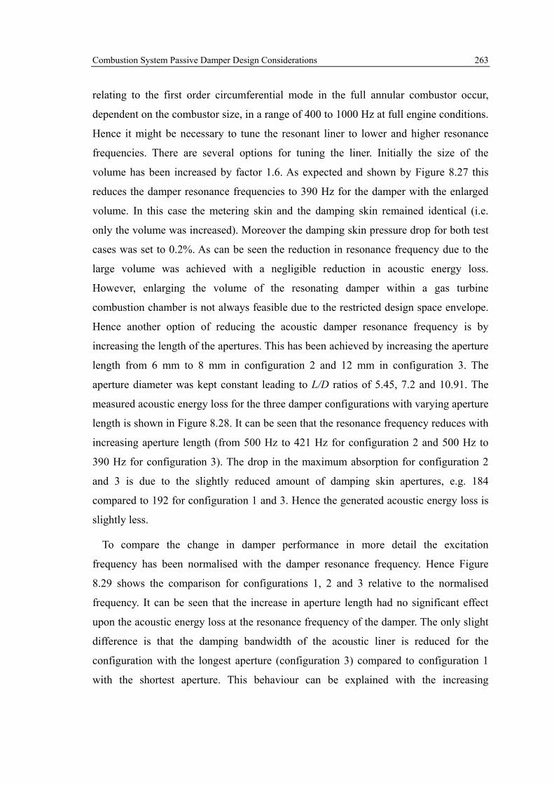
Combustion System Passive Damper Design Considerations 263
relating to the first order circumferential mode in the full annular combustor occur,
dependent on the combustor size, in a range of 400 to 1000 Hz at full engine conditions.
Hence it might be necessary to tune the resonant liner to lower and higher resonance
frequencies. There are several options for tuning the liner. Initially the size of the
volume has been increased by factor 1.6. As expected and shown by Figure 8.27 this
reduces the damper resonance frequencies to 390 Hz for the damper with the enlarged
volume. In this case the metering skin and the damping skin remained identical (i.e.
only the volume was increased). Moreover the damping skin pressure drop for both test
cases was set to 0.2%. As can be seen the reduction in resonance frequency due to the
large volume was achieved with a negligible reduction in acoustic energy loss.
However, enlarging the volume of the resonating damper within a gas turbine
combustion chamber is not always feasible due to the restricted design space envelope.
Hence another option of reducing the acoustic damper resonance frequency is by
increasing the length of the apertures. This has been achieved by increasing the aperture
length from 6 mm to 8 mm in configuration 2 and 12 mm in configuration 3. The
aperture diameter was kept constant leading to L/D ratios of 5.45, 7.2 and 10.91. The
measured acoustic energy loss for the three damper configurations with varying aperture
length is shown in Figure 8.28. It can be seen that the resonance frequency reduces with
increasing aperture length (from 500 Hz to 421 Hz for configuration 2 and 500 Hz to
390 Hz for configuration 3). The drop in the maximum absorption for configuration 2
and 3 is due to the slightly reduced amount of damping skin apertures, e.g. 184
compared to 192 for configuration 1 and 3. Hence the generated acoustic energy loss is
slightly less.
To compare the change in damper performance in more detail the excitation
frequency has been normalised with the damper resonance frequency. Hence Figure
8.29 shows the comparison for configurations 1, 2 and 3 relative to the normalised
frequency. It can be seen that the increase in aperture length had no significant effect
upon the acoustic energy loss at the resonance frequency of the damper. The only slight
difference is that the damping bandwidth of the acoustic liner is reduced for the
configuration with the longest aperture (configuration 3) compared to configuration 1
with the shortest aperture. This behaviour can be explained with the increasing

Combustion System Passive Damper Design Considerations 264
reactance for the longer apertures. The gradient for the damping system reactance as
shown for the three configurations in Figure 8.30 is steeper for the configurations with
longer apertures. Hence the bandwidth of the resonant damper is reduced at lower
frequencies.
The experimental results show that a resonating passive damper system can operate
more efficiently, in terms of acoustic energy loss compared with a non-resonant liner
system within the restricted space envelope of a gas turbine combustion system. Various
examples of tuning the resonant liner have been shown and analysed. However a further
objective of acquiring this data was to provide additional validation data for the
analytical models and derive some simple geometrical parameters for the tuning, design
and optimisation of a resonating damping system. This will be discussed in the
following sections.
8.3.2 Analytical Model Validation The developed analytical model described in section 8.1 will be compared to the
experimental results. In this case the prediction of the damper is more challenging due
to (i) the increased length of the aperture which was shown to be more challenging in
section 5.9 and (ii) the increased Strouhal numbers for some of the investigated
geometries. To be able to assess the mean flow loss coefficient accurately the discharge
coefficients were measured for the described liner configurations. In this case the total
damping system, metering skin and damping skin, was placed in a plenum and the total
effective area for the given damper configuration was measured. Simultaneously the
metering skin and damping skin pressure drop was also measured. Hence it was
possible to derive the effective area of the metering and damping skins and hence derive
their respective discharge coefficients. The measured discharge coefficients for each
resonating damper geometry are presented in Table 8.2. Moreover the length corrections
for the apertures in the damping skin were approximated from the length corrections
presented in Table 5.1 for the aperture length to diameter ratios of 3, 5, 6.8 and 10. In
addition the length correction defined for the aperture with L/D = 10 was also used for
the metering skin impedance model with L/D = 16.67.

Combustion System Passive Damper Design Considerations 265
Damper config-uration
Damping skin L/D
Damping skin dp/p in %
Damping skin CD
Metering skin CD
1 5.45 0.1% 0.69 0.58
1 5.45 0.16% 0.7 0.6
1 5.45 0.2% 0.72 0.6
2 7.27 0.14% 0.64 0.58
3 10.91 0.15% 0.58 0.58
4 5.45 0.1% 0.69 0.58
4 5.45 0.22% 0.72 0.6
5 3.75 0.03% 0.83 0.59 Table 8.2: Measured discharge coefficients for metering skin and damping skin for
the five investigated resonant damper configurations It was mentioned in section 5.9.1 that the measured mean flow discharge coefficient
deviated from the discharge coefficient derived from the acoustic model for apertures
with L/D longer than two. Moreover section 5.9.2 discussed additional sources of error
in the model due to the change of the aperture flow field and the development of orifice
internal boundary layers for the apertures longer than L/D of two. The previous section
showed good agreement between the developed analytical model for apertures of L/D ~
3. However to gain a better estimate of the accuracy of the prediction for even larger
L/D the measured discharge coefficient (as in Table 8.2) has been used and the model
described in section 8.1 was compared to the measured data in the previous section.
The resonant liner experiments were conducted in an impedance tube arrangement
with the damper perpendicular to the axial acoustic waves. Hence the measured results
are not affected by acoustic mode shapes as the pressure amplitude and phase along the
damper surface is constant. Therefore the measured pressure amplitude immediately
downstream of the damping skin at x = 0 was used as an input excitation amplitude into
the acoustic model and for the normalisation of the acoustic energy loss.
Figure 8.31 shows a comparison of the calculated and measured normalised acoustic
energy loss for the resonant damper configuration 1. It can be seen that the model
predicts the maximum acoustic loss at the same frequency as the experiment. In general
the predicted acoustic loss is showing the same trend as the experimental data. However
the maximum acoustic loss is estimated to be approximately 13% smaller than in the

Combustion System Passive Damper Design Considerations 266
experiment. Moreover the pressure amplitude ratio is showing the same characteristic as
the experimental data (Figure 8.32). In this case the predicted maximum amplitude ratio
is shifted to higher frequencies compared to the measurement and the maximum value is
approximately 8% smaller for the prediction. Finally the phase difference between the
cavity amplitude and the excitation amplitude is shown in Figure 8.33. It can be seen
that the trend of the phase difference predicted by the model is in agreement with the
experiment. Hence the frequency for the maximum calculated normalised acoustic loss
compared to the experimental data is in agreement in Figure 8.31. The reason for the
mismatch in pressure amplitude ratio and acoustic energy loss is caused by the
calculated impedance of the damping skin and the metering skin used in the model.
Hence the measured system impedance has been compared to the calculated impedance.
Note in this case the impedance was defined as the ratio between incident pressure
amplitude and the velocity amplitudes within the apertures of the damping skin
1
0
ˆˆ
Dup
Z = . ( 8.18)
The calculated and measured acoustic resistance is compared in Figure 8.34. The
predicted resistance is on average 20 % larger than the measured resistance. This
overestimate of the liner resistance is therefore causing a reduction in the acoustic
energy loss relative to the measured data (Figure 8.31.)
Figure 8.35 shows the comparison between the measured and predicted acoustic
reactance. It can be seen that the predicted reactance is in excellent agreement with the
measured reactance. This shows that the length correction estimates for the aperture
geometry in the liner was approximated correctly based on the aperture measurements
presented in section 5.9. The accurate prediction of the length correction for the liner
apertures is important for resonant liners and the calculation of the liner resonance
frequency. Currently an estimate on the length correction can be undertaken based on
measurements of similar orifice geometries or with semi-empirical length correction
estimates as they are shown in Bellucci et. al. (2004b). However, experimental
validation for the used geometry is still necessary. In this case the error in the acoustic
energy loss prediction is caused by the discrepancies in the resistance prediction which

Combustion System Passive Damper Design Considerations 267
is based on a viscosity model for the boundary layer within the aperture as well as on
the loss coefficient estimated from the mean flow discharge coefficient.
As Figure 8.36 shows the model captures the trend in acoustic energy loss with
varying pressure drop across the damping skin. In this case the measured discharge
coefficients for each pressure drop have been used in the analytical model to predict the
acoustic energy loss. The model shows a reduction in acoustic loss with increasing
mean pressure drop (from 0.1 to 0.2%). However it can be seen that the maximum
acoustic energy loss calculated by the analytical model is consistently underestimated.
Nevertheless the relative change in predicted energy loss for the three cases seems to
agree very well with the relative change in acoustic energy loss measured in the
experiment. Moreover the resonance frequencies are predicted at the correct frequency.
Figure 8.37 shows a comparison between the modelling and the experimental data
with a variation in damper volume with a damping skin mean pressure drop of 0.2%. It
can be seen that the modelling technique again captures the acoustic energy loss
characteristics. The change in resonance frequency due to the increased damper volume
is also captured very well. This also provides further evidence that the measured length
corrections in section 5.9 can be used for an initial estimate of the length correction and
resonance frequency prediction. Again the relative change in acoustic energy loss is
reproduced very well by the model, but the maximum energy loss is predicted to be
smaller than the experiment.
For the data presented the maximum loss is consistently under estimated by the
developed model due to the over prediction of the damping skin resistance. To
investigate this issue further the model has been used to compare acoustic damper
configurations 2 and 3. In this case the hole length of the damping skin apertures has
been increased. The comparison between the acoustic model and the measurement is
shown in Figure 8.38. This indicates that the acoustic loss prediction deviates further
away from the experimental data with increasing aperture length. For example the
deviation in the maximum acoustic loss is approximately 13%, 18% and 30% for L/D
ratios of 5.45, 7.27 and 10.91 respectively.
Figure 8.39 shows that the reactance prediction agrees very well with the measured
data apart for the geometry with L/D of 10.91. In this case the length correction is

Combustion System Passive Damper Design Considerations 268
overestimated for this geometry. However the discrepancies in acoustic energy loss is
caused by an over prediction of the acoustic resistance of the damping skin as it is
shown in Figure 8.40. It can be seen that the discrepancy between the measured and the
calculated resistance is increasing with increasing length-to-diameter ratio.
In general the model reproduces the acoustic energy loss characteristics for the
investigated damper experiments very well. This is encouraging and therefore the model
can be used to maximise acoustic dampers with larger aperture length-to-diameter ratio.
However the maximum acoustic energy loss is consistently underestimated by the
modelling method. The data suggests that this is caused by an overestimation for the
acoustic resistance and will be further investigated in the following section.
8.3.3 Sources of Errors in the Analytical Modelling for Apertures with Large Length-to-Diameter Ratios
As already discussed in section 5.9.2 the increased inaccuracies for large L/D ratio
apertures is caused by the complex interaction of the losses surrounding an aperture
with L/D ratios larger than two. The results in section 8.2.2 suggest that the model is
sufficient for apertures with L/D of 3 as the viscosity effects seem to be small. However
this is not the case for the resonating liner configurations with apertures longer than L/D
of 3.
Section 5.9.2 suggested two options to estimate the inflow and outflow losses as well
as the viscous losses within the aperture, as they are assessed against the experimental
data in this section. Initially the measured mean flow discharge coefficient is used
without including any viscosity term within the model for the resistance estimation. In
this case the reactance is still dependent on the unsteady viscosity model, i.e. only the
imaginary part in equation (5.34) is used. This approach is shown in Figure 8.41 for
damper configurations 1, 2 and 3 indicated as ‘Model 2’. In general predicted acoustic
absorption has increased and the difference between measurement and prediction has
reduced compared to the data presented in Figure 8.38. However significant deviations
remain for apertures with L/D of 10.91. It can be concluded that the inclusion of the
viscosity term in the resistance of the model increases the discrepancy to the
experimental data.

Combustion System Passive Damper Design Considerations 269
The second option as proposed in section 5.9.2 was also used to calculate the acoustic
energy loss for the three damper configurations as shown in Figure 8.42 indicated by
‘Model 3’. In this case it was assumed that the inflow and outflow losses were best
represented by the mean flow discharge coefficient of an aperture where the mean flow
is just attaching to the inside of the orifice, i.e. L/D of two. Hence the discharge
coefficient of 0.81 was used in this calculation. The effects of viscosity have been
included in the acoustic resistance and reactance calculation. It can be seen that this
approach significantly improved the accuracy of the acoustic energy loss prediction.
The calculated energy loss agrees well with damper configurations 1 and 2, and much
reduced discrepancies can also be seen for configuration 3. This seems to indicate that
this approach is the more representative method for the calculation of the acoustic loss
of long apertures. However as already mentioned in section 5.9.2 further research is
needed to understand the fundamental physics of the unsteady flow field for long
apertures to generate more reliable modelling techniques. This has technical relevance
as the application of long aperture length-to-diameter ratios is important to tune
resonant liners to aero-engine gas turbine combustion system representative
frequencies. In chapter 7 a method was presented capable of identifying unsteady flow
behaviour relevant to the acoustic absorption process. Hence this could be applied onto
CFD methods or sophisticated experimental setups resolving the relevant unsteady flow
characteristics of long L/D ratio apertures to develop a more reliable modelling
technique.
8.3.4 Resonance Parameter for Preliminary Damper Design During the initial design stages it would be useful to develop a simple relationship of
all the relevant geometric parameters of a resonant liner to establish the resonance
frequency of the damping device. Therefore a simple optimisation within the design
space envelope can be conducted to tune the passive damper onto the desired frequency.
In this work the method described by Hughes and Dowling (1990) was initially used to
assess the resonance frequency of the linear passive damping device. In their study they
have used the classic Helmholtz resonator equation as defined by Rayleigh (1899):

Combustion System Passive Damper Design Considerations 270
VK
k Dres = .
( 8.19)
Hence the wave number at the resonance frequency is defined by the square root of the
Rayleigh Conductivity divided by the resonator volume. Thus the resonance frequency
is defined as
VKc
f Dres π2
= . ( 8.20)
Comparing equation ( 8.20) with equation (1.13) shows that the Rayleigh Conductivity
for the Helmholtz resonator can be expressed as:
RLR
LAKeff
D 850
2
.+==
π . ( 8.21)
In the study by Hughes and Dowling (1990) a perforated liner backed by a resonating
volume was studied. Moreover the aim was to damp high frequency combustion
instabilities in afterburners (also known as screech). As the frequencies are large the
length of the apertures need to be short and in this case, can be neglected. Therefore the
Conductivity of a circular aperture with negligible aperture length and the absence of
mean flow can be expressed as (Rayleigh (1896), Hughes and Dowling (1990))
RKD 2= . ( 8.22)
This is also valid as a first approximation for the resonance frequency of a resonant
linear damper (initially ignoring the effect of the mean flow upon the Conductivity of
the aperture). Finally the cavity volume of the resonating liner needs to be defined. In
this case the passive damper is divided into multiple Helmholtz resonators. Hence each
aperture and its portion of the backing volume is regarded as a Helmholtz resonator.
Therefore the relevant volume can be estimated by using the cavity depth S and the
pitch between the apertures Pa:
SPV a2= . ( 8.23)
Substituting equations ( 8.22) and ( 8.23) into equation ( 8.19) leads to the wave
number at the resonance frequency for a perforated liner backed by a resonating cavity:

Combustion System Passive Damper Design Considerations 271
SP
Rk
ares 2
2= .
( 8.24)
Hughes and Dowling (1990) used this expression to define the resonance parameter
RSPk
Q ares2
22= .
( 8.25)
If this parameter is equal to one than the damper is tuned to the resonance frequency.
In the work of Hughes and Dowling (1990) equation ( 8.25) successfully enabled the
prediction of the resonance frequency and non-dimensionalised the frequency axis for
the conducted experiments. However, this work is aimed at frequencies that are
significantly lower than those associated with afterburner screech. Thus an elegant way
of reducing the resonance frequency, for a given damper porosity and limited volume, is
to increase the aperture length. This was the approach taken in this work to reduce the
resonance frequency of the acoustic damper. As Figure 8.43 shows the maximum
acoustic energy loss for each of the investigated geometries does not coincide with a Q-
parameter of one (based on the definition in Hughes and Dowling (1990)). Moreover
the phase between the incident and the cavity pressure amplitude, which is 90° at
resonance, is also not coinciding with a Q-parameter of one at 90° (Figure 8.44). This
mismatch is due to the additional aperture length, which was negligible in the work of
Hughes and Dowling (1990) but needs to be included in this work. Hence the resonance
parameter has been modified using a length correction as defined in Stow and Dowling
(2003):
effeffeffD
DD LR
R
R
LR
R
R
LK
KK
22
21
2
1
2
22+
=+
=+
=π
π
ππ
. ( 8.26)
Therefore the aperture length corrected Q-parameter can be defined by substituting
equation ( 6.17) into equation ( 6.10):
222
22
2
2
R
LRSPk
KSPk
Q effares
D
aresL
π
π +== .
( 8.27)

Combustion System Passive Damper Design Considerations 272
This parameter was successfully used with resonant acoustic damper data presented in
Rupp and Carrotte (2011). However, this parameter is only valid for perforated liners
backed by a rigid wall, e.g. Hughes and Dowling (1990). Hence equation ( 8.27) needs
to be extended to a double liner system, i.e. the damping liner is backed by a metering
skin instead of a rigid wall. This extension can be conducted using the formula to
calculate the resonance frequency of a Helmholtz resonator with two apertures
connected to the resonator volume as, for example, defined by Keller and Zauner (1995)
+=
2
2
1
112 L
ALA
Vcfres π
. ( 8.28)
In this case the resonance frequency is a function of both areas (damping skin and
metering skin) and the effective length of their apertures. Hence using equations ( 8.20)
and ( 8.23) the wave number at resonance can be defined based on two aperture
Conductivities
222
121
2 11D
aD
ares K
SPK
SPk
,,
+= , ( 8.29)
where 1 denotes the damping skin and 2 denotes the metering skin. The pitch between
the apertures can be defined using the porosity of the damping and metering skin
assuming a square pattern orifice array in the liner
l
jja
RP
σ
π 2=, for 21,=j .
( 8.30)
Note the hole pattern in this work was not an exact square pattern thus the pitch
calculated by equation ( 8.30) is an effective pitch sufficient for the calculation of the
resonance parameter. Hence the modified resonance parameter for resonant acoustic
dampers with two perforated liners relevant to combustion system liners can be defined
as
222
121
2
2 11D
aD
a
resL
KSP
KSP
kQ
,,
+= .
( 8.31)

Combustion System Passive Damper Design Considerations 273
Figure 8.45 shows the measured normalised acoustic energy loss for the five
investigated damper configurations. In this case the modified resonance parameter was
calculated using the same effective aperture length assumptions as for the analytical
model in the previous section. It can be seen that the maximum acoustic energy loss
occurs at a modified resonance parameter equal to one for all geometries. Moreover the
measured phase difference between cavity and excitation pressure amplitude, shown in
Figure 8.46, is also showing 90° phase difference for the modified resonance parameter.
This is further proof that the resonance condition is predicted correctly by the modified
version of the parameter.
Hence the simple relationship of geometric parameters and damper operating
conditions, as defined in equation ( 8.31) for the modified resonance parameter, can be
used to define a resonating acoustic damper geometry tuned to the relevant combustion
instability frequency.
8.4 Hot Gas Ingestion As described in Rupp et. al. (2012) the ingestion of hot gases from the combustor into
the damper volume is of concern during the design of passive dampers. This ingestion
of hot gas can arise both from the time averaged and time dependent flow field
characteristics. The following description of the phenomena can also be found in Rupp
et. al. (2012).
The mean pressure drop across the damping skin means that on a spatially averaged
basis the pressure within the damper cavity is greater than the flame tube pressure i.e. so
relatively cool gas flows through the damping skin and into the combustor and no hot
gas ingestion occurs. However, locally the mean pressure distribution will vary across
the damper surface, as shown in Figure 8.2, resulting in the potential for hot gas to
locally flow into the damper cavity. Hence as the mean pressure drop across the
damping skin is reduced so the likelihood for local hot gas ingestion increases. However
this process can be predicted by time averaged numerical (CFD) prediction of the flow
field. Also of concern, though, and of primary interest here is the time dependent
ingestion of hot gas into the damper cavity due to the unsteady flow field.

Combustion System Passive Damper Design Considerations 274
As the magnitude of the unsteady pressure amplitudes inside the combustor increases
so there is the potential for flow to reverse through the damping skin orifices on a time
dependent basis i.e. so that hot gas is ingested at certain phases of the acoustic cycle.
However, this can be investigated using the developed 1D analytical model in terms of
- assessing the robustness of different damper designs to gas ingestion and
- at what level of pressure oscillations within the combustor will hot gas ingestion
commence.
As the velocity perturbation in the damping holes tends to the mean velocity hot gas
ingestion will occur (i.e. 11 DD Uu ~1). However, this also corresponds to the operating
condition where the acoustic absorption transitions into the non-linear regime. It was
shown in the analysis of the acoustic absorption experiments in section 6.4.1 that non-
linear absorption occurs for unsteady to mean velocity ratios of approximately 0.4 and
greater. Therefore the model can be used to identify at which excitation pressure
amplitudes non-linear absorption occurs. This not only indicates the operating condition
where the analytical model becomes invalid (i.e. since the linear absorption model is no
longer valid), but this can also be used to provide a design margin against hot gas
ingestion.
Figure 8.47 shows the unsteady velocity amplitude normalised with the mean velocity
across the damping skin for three different liner separations for the non-resonant liner
geometry described in section 8.2. Note that the magnitude of the excitation pressure
0p is normalised with the absolute mean pressure inside the main duct 0p . For the
largest cavity depth (S/H = 0.67) it can be seen that the orifice perturbation ( )1u is
reaching the onset of non-linear absorption for an excitation amplitude of approximately
0.5% of the combustion chamber pressure. For example, at 40 bar this would equate to
an excitation amplitude of 177 dB. However as the cavity depth decreases so less
acoustic energy is absorbed and the velocity perturbation ( )1u , for a given excitation
amplitude, decreases. Hence with decreasing cavity depth the damper becomes more
robust to time dependant hot gas ingestion but absorbs less energy. In this way both the
relative sensitivity of different configurations to hot gas ingestion can be assessed along
with the unsteady pressure amplitudes at which this will occur.

Combustion System Passive Damper Design Considerations 275
As expected a resonant liner is more prone to hot gas ingestion due to the high
unsteady velocity amplitudes. This can be seen, for example, in Figure 8.48 for the
resonant damper configuration 1. In this case the transition from linear to non-linear
absorption occurs at an equivalent sound pressure of 168 dB at 40 bar combustor inlet
pressure. This highlights the importance of accurate non-linear acoustic modelling as
the resonant dampers are operating close to the transition range within gas turbine
combustors.
As already discussed the current modelling for the transition from linear to non-linear
acoustic absorption is assuming a velocity amplitude ratio of one for the onset to non-
linear absorption. Hence for a given geometry a curve fit to the measured velocity
amplitude should enable a more accurate assessment of the onset to hot gas ingestion
which occurs at velocity amplitude ratios of approximately one. Hence the current
design tool is giving a pessimistic assessment of the onset of hot gas ingestion into the
damper cavity.
8.5 Closure This chapter has discussed a set of design tools developed during this work:
• a simple parameter which enables the preliminary design and tuning for the
geometric parameters of a multi-liner resonating damping system,
• an analytical model to estimate the acoustic energy loss of acoustic dampers
with a high accuracy for apertures up to a length-to-diameter ratio of 3 (larger
L/D ratios are possible with reduced accuracy),
• an impedance methodology to investigate the interaction and optimisation of
isolated acoustic components such as fuel injectors or acoustic dampers,
• a prediction and scaling method to investigate the risk of hot gas ingestion due to
the unsteady velocity amplitudes within the damping skin.
The developed tool set enables a comprehensive preliminary design of non-resonant
and resonant acoustic absorbers with multiple perforated liners within a gas turbine
combustion system. Moreover the model has been extended to assess the impact of

Combustion System Passive Damper Design Considerations 276
circumferential waves (appendix E). Finally the analytical model can also be used as a
development platform for aperture Rayleigh Conductivity models.
It has been shown that the bulk acoustic modelling is independent of complex flow
characteristics downstream of the apertures. Hence cross-flow influence and complex
swirling flow fields across the downstream end of the damping skins had no significant
effect. This can be concluded from the excellent agreement of the experimental non-
resonating damper data compared to the linear acoustic model which does not include
any cross flow effects upon the damping skins. Using the methods for the hot gas
ingestion analysis it has been shown that the liners with increased unsteady pressure
drop, such as large volume non-resonant liners and resonating dampers, are more prone
to hot gas ingestion due to the larger unsteady velocity amplitudes for a given pressure
amplitude. The analytical modelling of long L/D apertures has shown discrepancies with
the measured data. It has been discussed that this is caused by the rather complex flow
field through the longer apertures with unsteady inflow profiles, boundary layer and
outflow effects. Some short term solutions have been shown to improve the accuracy.
However it is recommended to investigate the unsteady flow physics of larger L/D
apertures in the future to improve the modelling accuracy for this technically relevant
application.
Experimental investigations into non-resonant liner systems have shown that the
design of efficient liners would necessitate large cavity volumes between the metering
and damping skins. Hence the absorption was maximised for plenum conditions in the
said cavity. Unfortunately this would not fit in the design space envelope for an aero-
engine gas turbine combustion system without unacceptable increases in weight of the
engine. Hence other damping options such as resonating acoustic dampers have been
investigated experimentally. It was demonstrated that the resonance effect can greatly
enhance the absorption of the applied acoustic dampers. Thus the application of such a
device shows a better acoustic damping performance within the given space envelope.
However the device needs tuning which can only be accurately done if the length
corrections of the apertures in the metering and damping skin are known. Moreover the
relevant frequencies occurring in aero gas turbine combustion systems make it
necessary to use rather large L/D ratio apertures in the damping skin.
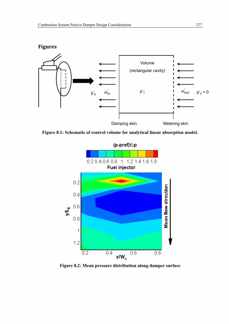
Combustion System Passive Damper Design Considerations 277
Figures
Metering skin
Volume
(rectangular cavity)
p’2 = 0p’1p’0'inm
'outm
Damping skin
Figure 8.1: Schematic of control volume for analytical linear absorption model.
Figure 8.2: Mean pressure distribution along damper surface

Combustion System Passive Damper Design Considerations 278
Figure 8.3: Pressure amplitude mode shape example
0.10
0.15
0.20
0.25
0.30
0.35
0.40
0.45
0.50
200 220 240 260 280 300 320 340 360 380 400 420
Ref
lect
ion
coef
ficie
nt -
|RC|2
Frequency in Hz
No damper
Metering Skin only
Metering Skin and Damping Skin S/H = 0.125
Figure 8.4: Comparison of measured reflection coefficients

Combustion System Passive Damper Design Considerations 279
0.00
0.05
0.10
0.15
0.20
0.25
0.30
0.35
0.40
0.45
0.50
200 220 240 260 280 300 320 340 360 380 400 420
Ref
lect
ion
coef
ficie
nt -
|RC|2
Frequency in Hz
No damper
S/H = 0.125
S/H = 0.25
S/H = 0.33
S/H = 0.46
S/H = 0.74
S/H = 1.35
S/H = 1.46
Figure 8.5: Reflection coefficients of various liner separations
0.0
0.1
0.2
0.3
0.4
0.5
0.6
0.7
0.8
0.9
1.0
0.0 0.1 0.2 0.3 0.4 0.5 0.6 0.7 0.8 0.9 1.0
Nor
mal
ised
Pre
ssur
e Am
plitu
de
y/LD
250Hz
300Hz
350Hz
Figure 8.6: Normalised mode shape pressure amplitudes at various frequencies

Combustion System Passive Damper Design Considerations 280
0.0
1.0
2.0
3.0
4.0
5.0
6.0
7.0
8.0
9.0
10.0
230 250 270 290 310 330 350 370 390 410
Nor
mal
ised
aco
ustic
ene
rgy
loss
-Π
P
Frequency in Hz
Exp. S/H 0.125
Model S/H = 0.125
Exp S/H = 0.33
Model S/H = 0.33
Exp = S/H = 1.56
Model S/H = 1.56
x10-6
Figure 8.7: Normalised acoustic loss comparison between experiment and analyti-
cal model with pressure mode shape input function
0.00
0.01
0.02
0.03
0.04
0.05
0.06
0.07
0.08
230 250 270 290 310 330 350 370 390 410
Acou
stic
ene
rgy
loss
-Π
Lin
J/s
Frequency in Hz
Exp. S/H 0.125
Model S/H = 0.125
Exp S/H = 0.33
Model S/H = 0.33
Exp = S/H = 1.56
Model S/H = 1.56
Figure 8.8: Acoustic energy loss comparison between experiment and modified
model with pressure mode shape input function

Combustion System Passive Damper Design Considerations 281
0.0
0.1
0.2
0.3
0.4
0.5
0.6
0.7
0.8
0.9
1.0
230 250 270 290 310 330 350 370 390 410Frequency in Hz
Exp. S/H = 0.33
Model S/H = 0.33
Exp. S/H = 0.46
Model S/H = 0.46
Exp. S/H = 0.74
Model S/H = 0.74
Exp. S/H = 1.35
Model S/H = 1.35
Pres
sure
am
plitu
de ra
tio -
|p1|/
|p0|
^^
Figure 8.9: Cavity pressure ratio comparison between the experiment (Exp.) and
the model
-90.0
-80.0
-70.0
-60.0
-50.0
-40.0
-30.0
-20.0
-10.0
0.0
230 250 270 290 310 330 350 370 390 410
Cav
ity P
hase
diff
eren
ce in
deg
rees
Frequency in Hz
Exp. S/H = 0.33
Model S/H = 0.33
Exp. S/H = 0.46
Model S/H = 0.46
Exp. S/H = 0.74
Model S/H = 0.74
Exp. S/H = 1.35
Model S/H = 1.35
Figure 8.10: Phase difference between cavity pressure amplitude and incident
pressure amplitude

Combustion System Passive Damper Design Considerations 282
0.0
0.1
0.2
0.3
0.4
0.5
0.6
0.7
0.8
0.9
1.0
0.00 0.25 0.50 0.75 1.00 1.25 1.50 1.75 2.00S/H
Experiment
Model
Pres
sure
am
plitu
de ra
tio -
|p1|/
|p0|
^^
Figure 8.11: Cavity pressure ratio variation with liner separation, experiment with
fuel injector
-80.0
-70.0
-60.0
-50.0
-40.0
-30.0
-20.0
-10.0
0.0
0.00 0.25 0.50 0.75 1.00 1.25 1.50 1.75 2.00
Phas
e di
ffere
nce
in d
egre
es
S/H
Experiment
Model
Figure 8.12: Phase angle between cavity pressure amplitude and excitation pres-
sure amplitude, experiment with fuel injector

Combustion System Passive Damper Design Considerations 283
0.00
0.02
0.04
0.06
0.08
0.10
0.12
0.14
0.00 0.25 0.50 0.75 1.00 1.25 1.50 1.75 2.00S/H
Damping skin
Metering skin|u
1|/U
D,1
and
|u2|/
UD
,2^
_^
_
Figure 8.13: Unsteady velocity amplitudes with varying liner separation
0.00
0.01
0.02
0.03
0.04
0.05
0.00 0.01 0.02 0.03 0.04 0.05
Adm
ittan
ce -
δ
Strouhal number - St
Damping skin
Metering skin
Figure 8.14: Calculated damping and metering skin admittance for S/H = 0.125

Combustion System Passive Damper Design Considerations 284
0.0
0.5
1.0
1.5
2.0
2.5
3.0
3.5
4.0
4.5
5.0
0.00% 0.25% 0.50% 0.75% 1.00% 1.25% 1.50% 1.75% 2.00%
Nor
mal
ised
aco
ustic
ene
rgy
loss
-Π
P
dp/p
S/H = 0.125
S/H = 0.33
S/H = 0.67
x10-6
Figure 8.15: Normalised loss for varying damping skin mean pressure drop
0.0
0.1
0.2
0.3
0.4
0.5
0.6
0.7
0.8
0.9
1.0
0.00% 0.25% 0.50% 0.75% 1.00% 1.25% 1.50% 1.75% 2.00%dp/p
S/H = 0.125
S/H = 0.33
S/H = 0.67
Pres
sure
am
plitu
de ra
tio -
|p1|/
|p0|
^^
Figure 8.16: Cavity pressure ratio with varying damping skin mean pressure drop

Combustion System Passive Damper Design Considerations 285
y/LD = 0Ztot
ZD
Zinj Zinj
Atot
ZD
Ztot
Schematic of test section Acoustic system impedances Acoustic branches
Figure 8.17: Schematic of non-resonant damper test section as a system of acoustic
branches.
0
200
400
600
800
1000
1200
1400
1600
1800
2000
0 100 200 300 400 500 600
Fuel
Inje
ctor
impe
danc
e -Z
inj
Frequency in Hz
Resistance
Reactance
Model Resistance
Model reactance
Figure 8.18: Fuel injector impedance.
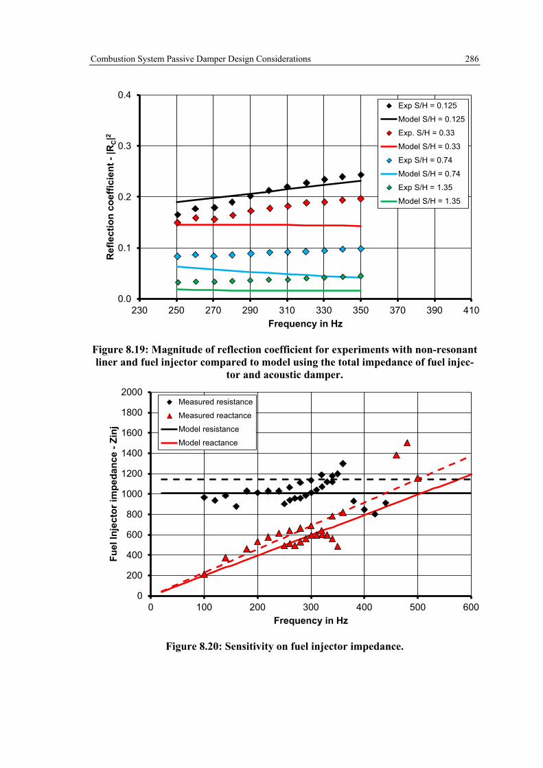
Combustion System Passive Damper Design Considerations 286
0.0
0.1
0.2
0.3
0.4
230 250 270 290 310 330 350 370 390 410
Ref
lect
ion
coef
ficie
nt -
|RC|2
Frequency in Hz
Exp S/H = 0.125
Model S/H = 0.125
Exp. S/H = 0.33
Model S/H = 0.33
Exp S/H = 0.74
Model S/H = 0.74
Exp S/H = 1.35
Model S/H = 1.35
Figure 8.19: Magnitude of reflection coefficient for experiments with non-resonant liner and fuel injector compared to model using the total impedance of fuel injec-
tor and acoustic damper.
0
200
400
600
800
1000
1200
1400
1600
1800
2000
0 100 200 300 400 500 600
Fuel
Inje
ctor
impe
danc
e -Z
inj
Frequency in Hz
Measured resistance
Measured reactance
Model resistance
Model reactance
Figure 8.20: Sensitivity on fuel injector impedance.
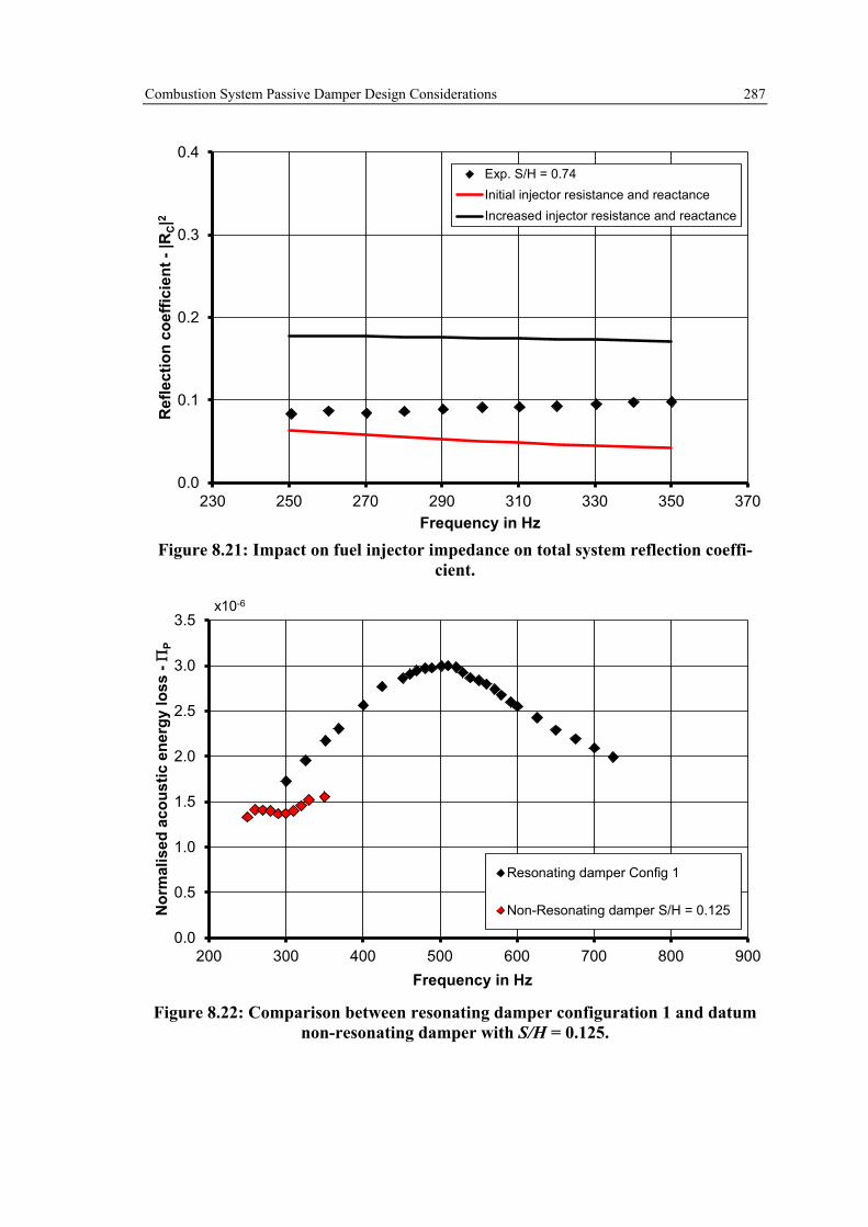
Combustion System Passive Damper Design Considerations 287
0.0
0.1
0.2
0.3
0.4
230 250 270 290 310 330 350 370
Ref
lect
ion
coef
ficie
nt -
|RC|2
Frequency in Hz
Exp. S/H = 0.74Initial injector resistance and reactanceIncreased injector resistance and reactance
Figure 8.21: Impact on fuel injector impedance on total system reflection coeffi-
cient.
0.0
0.5
1.0
1.5
2.0
2.5
3.0
3.5
200 300 400 500 600 700 800 900
Nor
mal
ised
aco
ustic
ene
rgy
loss
-Π
P
Frequency in Hz
Resonating damper Config 1
Non-Resonating damper S/H = 0.125
x10-6
Figure 8.22: Comparison between resonating damper configuration 1 and datum
non-resonating damper with S/H = 0.125.

Combustion System Passive Damper Design Considerations 288
0.0
0.3
0.6
0.9
1.2
1.5
100 300 500 700 900Frequency in Hz
|p1|/
|p0|
^^
-150
-120
-90
-60
-30
0
100 300 500 700 900
Phas
e di
ffere
nce
in d
egre
es
Frequency in Hz Figure 8.23: Pressure amplitude ratio and phase difference between damper cavity
and excitation pressure amplitude for damper configuration 1.
-30
-20
-10
0
10
20
30
40
200 300 400 500 600 700 800 900
Rea
ctan
ce -
Im(Z
)
Frequency in Hz
Figure 8.24: Acoustic reactance of damper configuration 1.

Combustion System Passive Damper Design Considerations 289
0.0
0.5
1.0
1.5
2.0
2.5
200 300 400 500 600 700 800 900Frequency in Hz
|p1-
p 0|2 / |
p 0|2
^^
^
Figure 8.25: Unsteady pressure difference across damping skin for damper config-
uration 1.
0.0
0.5
1.0
1.5
2.0
2.5
3.0
3.5
4.0
4.5
200 300 400 500 600 700 800 900
Nor
mal
ised
aco
ustic
ene
rgy
loss
-Π
P
Frequency in Hz
dp/p = 0.2%dp/p = 0.16%dp/p = 0.1%
x10-6
Figure 8.26: Variation of mean pressure drop across the damping skin for resonat-
ing damper configuration 1.

Combustion System Passive Damper Design Considerations 290
0.0
0.5
1.0
1.5
2.0
2.5
3.0
3.5
200 300 400 500 600 700 800 900
Nor
mal
ised
aco
ustic
ene
rgy
loss
-Π
P
Frequency in Hz
Config 1: Liner separation 64.7mm
Config 4: Liner separation 104.7mm
x10-6
Figure 8.27: Comparison for two resonating dampers with enlarged cavity volume.
0.0
0.5
1.0
1.5
2.0
2.5
3.0
3.5
200 300 400 500 600 700 800 900
Nor
mal
ised
aco
ustic
ene
rgy
loss
-Π
P
Frequency in Hz
Config 1: L/D = 5.45Config 2: L/D = 7.27Config 3: L/D = 10.91
x10-6
Figure 8.28: Normalised acoustic energy loss comparison of damper configuration 1, 2 and 3 with effective length variation for damping skin pressure drop of dp/p =
0.15%.

Combustion System Passive Damper Design Considerations 291
0.0
0.5
1.0
1.5
2.0
2.5
3.0
3.5
0.2 0.4 0.6 0.8 1 1.2 1.4 1.6 1.8
Nor
mal
ised
aco
ustic
ene
rgy
loss
-Π
P
Normalied frequency - Fres/F
Config 1: L/D = 5.45Config 2: L/D = 7.27Config 3: L/D = 10.91
x10-6
Figure 8.29: Normalised acoustic energy loss comparison of damper configuration
1, 2 and 3 relative to the normalised frequency, damping skin pressure drop of dp/p = 0.15%.
-50
-40
-30
-20
-10
0
10
20
30
40
50
0.2 0.4 0.6 0.8 1 1.2 1.4 1.6 1.8
Rea
ctan
ce -
Im(Z
)
Normalied frequency - Fres/F
Config 1: L/D = 5.45Config 2: L/D = 7.27Config 3: L/D = 10.91
Figure 8.30: Measured acoustic reactance for configuration 1, 2 and 3 relative to
the normalised frequency, damping skin pressure drop of dp/p = 0.15%.
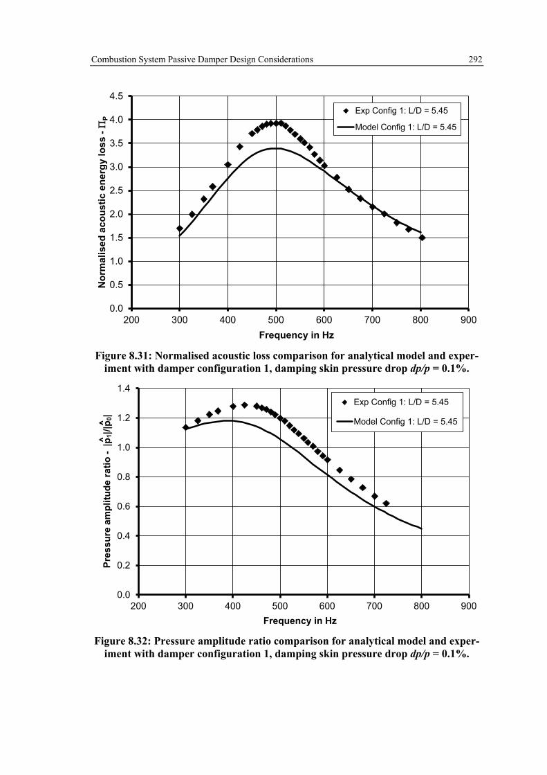
Combustion System Passive Damper Design Considerations 292
0.0
0.5
1.0
1.5
2.0
2.5
3.0
3.5
4.0
4.5
200 300 400 500 600 700 800 900
Nor
mal
ised
aco
ustic
ene
rgy
loss
-Π
P
Frequency in Hz
Exp Config 1: L/D = 5.45
Model Config 1: L/D = 5.45
Figure 8.31: Normalised acoustic loss comparison for analytical model and exper-
iment with damper configuration 1, damping skin pressure drop dp/p = 0.1%.
0.0
0.2
0.4
0.6
0.8
1.0
1.2
1.4
200 300 400 500 600 700 800 900Frequency in Hz
Exp Config 1: L/D = 5.45
Model Config 1: L/D = 5.45
Pres
sure
am
plitu
de ra
tio -
|p1|/
|p0|
^^
Figure 8.32: Pressure amplitude ratio comparison for analytical model and exper-
iment with damper configuration 1, damping skin pressure drop dp/p = 0.1%.

Combustion System Passive Damper Design Considerations 293
-150
-120
-90
-60
-30
0
200 300 400 500 600 700 800 900
Phas
e di
ffere
nce
in d
egre
es
Frequency in Hz
Exp Config 1: L/D = 5.45
Model Config 1: L/D = 5.45
Figure 8.33: Phase difference between cavity pressure amplitude and excitation
amplitude calculated by the analytical model and compared to the experiment with damper configuration 1, damping skin pressure drop dp/p = 0.1%.
0
5
10
15
20
25
30
35
200 300 400 500 600 700 800 900
Res
ista
nce
-Re(
Z)
Frequency in Hz
Exp Config 1: L/D = 5.45
Model Config 1: L/D = 5.45
Figure 8.34: Comparison of measured and calculated acoustic resistance for acous-
tic damper configuration 1, damping skin pressure drop dp/p = 0.1%.

Combustion System Passive Damper Design Considerations 294
-40
-30
-20
-10
0
10
20
30
40
200 300 400 500 600 700 800 900
Rea
ctan
ce -
Im(Z
)
Frequency in Hz
Exp Config 1: L/D = 5.45
Model Config 1: L/D = 5.45
Figure 8.35: Comparison of measured and calculated acoustic reactance for acous-
tic damper configuration 1, damping skin pressure drop dp/p = 0.1%.
0.0
0.5
1.0
1.5
2.0
2.5
3.0
3.5
4.0
4.5
200 300 400 500 600 700 800 900
Nor
mal
ised
aco
ustic
ene
rgy
loss
-Π
P
Frequency in Hz
Exp dp/p = 0.1%Model dp/p = 0.1%Exp dp/p = 0.15%Model dp/p = 0.15%Exp dp/p = 0.2%Model dp/p = 0.2%
x10-6
Figure 8.36: Comparison of measured and calculated acoustic energy loss with
changing mean pressure drop across the damping skin for damper configuration 1.

Combustion System Passive Damper Design Considerations 295
0.0
0.5
1.0
1.5
2.0
2.5
3.0
3.5
200 300 400 500 600 700 800 900
Nor
mal
ised
aco
ustic
ene
rgy
loss
-Π
P
Frequency in Hz
Exp Config 1: Liner separation 64.7mm
Model Config 1: Liner separation 64.7mm
Exp Config 4: Liner separation 104.7mm
Model Config 4: Liner separation 104.7mm
x10-6
Figure 8.37: Comparison of measured and calculated acoustic energy loss for
damper configuration 1 and 4. Damping skin pressure drop dp/p = 0.2%.
0.0
0.5
1.0
1.5
2.0
2.5
3.0
3.5
200 300 400 500 600 700 800 900
Nor
mal
ised
aco
ustic
ene
rgy
loss
-Π
P
Frequency in Hz
Exp Config 1: L/D = 5.45Model Config 1: L/D = 5.45Exp Config 2: L/D = 7.27Model Config 2: L/D = 7.27Exp Config 3: L/D = 10.91Model Config 3: L/D = 10.91
x10-6
Figure 8.38: Comparison of measured and calculated acoustic energy loss for damper configuration 1, 2 and 3. Damping skin pressure drop dp/p = 0.15%.

Combustion System Passive Damper Design Considerations 296
-60
-50
-40
-30
-20
-10
0
10
20
30
40
50
100 200 300 400 500 600 700 800 900
Rea
ctan
ce -
Im(Z
)
Frequency in Hz
Exp Config 1: L/D = 5.45Model Config 1: L/D = 5.45Exp Config 2: L/D = 7.27Model Config 2: L/D = 7.27Exp Config 3: L/D = 10.91Model Config 3: L/D = 10.91
Figure 8.39: Comparison of measured and calculated acoustic reactance for damp-
er configuration 1, 2 and 3. Damping skin pressure drop dp/p = 0.15%.
0
10
20
30
40
50
60
70
80
100 200 300 400 500 600 700 800 900
Res
ista
nce
-Re(
Z)
Frequency in Hz
Exp Config 1: L/D = 5.45Model Config 1: L/D = 5.45Exp Config 2: L/D = 7.27Model Config 2: L/D = 7.27Exp Config 3: L/D = 10.91Model Config 3: L/D = 10.91
Figure 8.40: Comparison of measured and calculated acoustic resistance for damper configuration 1, 2 and 3. Damping skin pressure drop dp/p = 0.15%.

Combustion System Passive Damper Design Considerations 297
0.0
0.5
1.0
1.5
2.0
2.5
3.0
3.5
200 300 400 500 600 700 800 900
Nor
mal
ised
aco
ustic
ene
rgy
loss
-Π
P
Frequency in Hz
Exp Config 1: L/D = 5.45
Model 2 Config 1: L/D = 5.45
Exp Config 2: L/D = 7.27
Model 2 Config 2: L/D = 7.27
Exp Config 3: L/D = 10.91
Model 2 Config 3: L/D = 10.91
x10-6
Figure 8.41: Comparison of measured and calculated normalised acoustic energy
loss damper configuration 1 to 3 using modelling option 2.
0.0
0.5
1.0
1.5
2.0
2.5
3.0
3.5
200 300 400 500 600 700 800 900
Nor
mal
ised
aco
ustic
ene
rgy
loss
-Π
P
Frequency in Hz
Exp Config 1: L/D = 5.45
Model 3 Config 1: L/D = 5.45
Exp Config 2: L/D = 7.27
Model 3 Config 2: L/D = 7.27
Exp Config 3: L/D = 10.91
Model 3 Config 3: L/D = 10.91
x10-6
Figure 8.42: Comparison of measured and calculated normalised acoustic energy
loss damper configuration 1 to 3 using modelling option 3.

Combustion System Passive Damper Design Considerations 298
L/D variation
0.0
0.5
1.0
1.5
2.0
2.5
3.0
3.5
0 0.1 0.2 0.3 0.4
Acou
stic
ene
rgy
loss
-Π
P
Q-Parameter
Config 1
Config 2
Config 3
x10-6
Damper volume variation
0.0
0.5
1.0
1.5
2.0
2.5
3.0
3.5
0 0.1 0.2 0.3 0.4Ac
oust
ic e
nerg
y lo
ss -
ΠP
Q-Parameter
Config 1
Config 4
x10-6
Figure 8.43: Measured normalised acoustic energy loss resonating liner experi-
ments compared to resonance parameter assessment.
L/D variation
-150
-120
-90
-60
-30
0
0 0.1 0.2 0.3 0.4
Phas
e di
ffere
nce
in d
egre
es
Q-Parameter
Config 1
Config 2
Config 3
Damper volume variation
-150
-120
-90
-60
-30
0
0 0.1 0.2 0.3 0.4
Phas
e di
ffere
nce
in d
egre
es
Q-Parameter
Config 1
Config 4
Figure 8.44: Phase of resonating liner experiments compared to resonance param-
eter assessment.
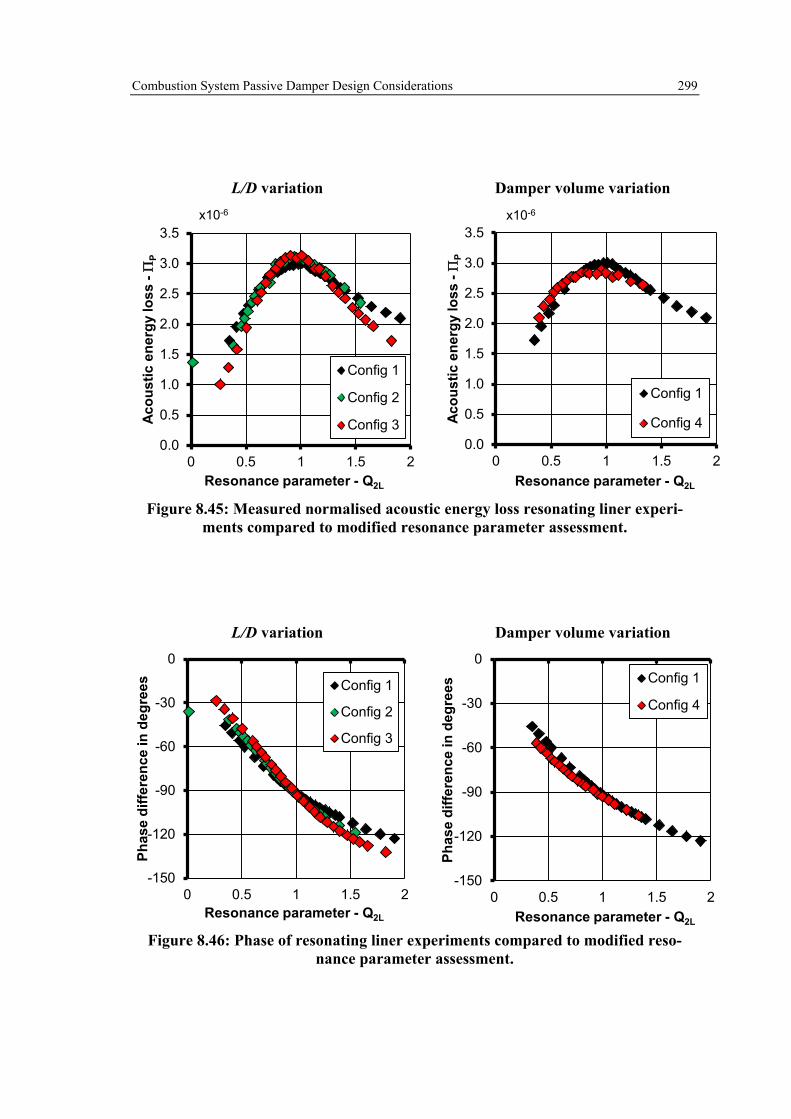
Combustion System Passive Damper Design Considerations 299
L/D variation
0.0
0.5
1.0
1.5
2.0
2.5
3.0
3.5
0 0.5 1 1.5 2
Acou
stic
ene
rgy
loss
-Π
P
Resonance parameter - Q2L
Config 1
Config 2
Config 3
x10-6
Damper volume variation
0.0
0.5
1.0
1.5
2.0
2.5
3.0
3.5
0 0.5 1 1.5 2Ac
oust
ic e
nerg
y lo
ss -
ΠP
Resonance parameter - Q2L
Config 1
Config 4
x10-6
Figure 8.45: Measured normalised acoustic energy loss resonating liner experi-
ments compared to modified resonance parameter assessment.
L/D variation
-150
-120
-90
-60
-30
0
0 0.5 1 1.5 2
Phas
e di
ffere
nce
in d
egre
es
Resonance parameter - Q2L
Config 1
Config 2
Config 3
Damper volume variation
-150
-120
-90
-60
-30
0
0 0.5 1 1.5 2
Phas
e di
ffere
nce
in d
egre
es
Resonance parameter - Q2L
Config 1
Config 4
Figure 8.46: Phase of resonating liner experiments compared to modified reso-
nance parameter assessment.

Combustion System Passive Damper Design Considerations 300
0.0
0.2
0.4
0.6
0.8
1.0
1.2
1.4
1.6
1.8
2.0
0.0% 1.0% 2.0% 3.0% 4.0% 5.0%
S/H = 0.125S/H = 0.33S/H = 0.67
Onset of non-linear absorption
|u1|/
UD
1^
_
|p0|/ p0^ _
Figure 8.47: Estimate of pressure amplitude for hot gas ingestion non-resonant
liner geometry.
0.0
0.2
0.4
0.6
0.8
1.0
1.2
1.4
1.6
1.8
2.0
0.0% 0.2% 0.4% 0.6% 0.8% 1.0%
Onset of non-linear absorption
|u1|/
UD
1^
_
|p0|/ p0^ _
Figure 8.48: Estimate of pressure amplitude for hot gas ingestion resonant liner
configuration 1, damping skin dp/p = 0.2%.

Conclusions and Recommendations 301
9 Conclusions and Recommendations The overall objective of this thesis was to establish the amount of acoustic energy
absorption associated with apertures that can be applied within a practical engineering
environment. In this work in particular the acoustic absorption characteristics of orifice
geometries typically found in a gas turbine combustion system have been investigated.
Initially single aperture isothermal experiments have been conducted to investigate the
acoustic energy loss for various orifices in the linear and non-linear acoustic absorption
regimes. These experiments have been used to assess the performance of current
acoustic absorption modelling methods and further the understanding of linear and non-
linear acoustic absorption. Particle image velocimetry measurements have been
conducted to capture the unsteady flow field generated in the presence of acoustic
waves to aid the investigation into the fundamental characteristics associated with the
acoustic absorption process. A methodology has been developed to identify the relevant
flow field features associated with the acoustic energy loss. The method has been
validated by comparing the kinetic energy flux of the acoustically related flow field to
the measured acoustic energy loss.
9.1 Experimental Measurements In general the acoustic absorption of an aperture is a function of the unsteady velocity
amplitude within the aperture (i.e. the larger the velocity amplitude the larger the
acoustic absorption for a given incident pressure amplitude). For the linear acoustic
absorption regime, within the Strouhal number range relevant to aero-engine
combustion systems, it has been shown that the acoustic energy loss varies with aperture
length-to-diameter ratio and this also reflects changes in the mean flow discharge
coefficient. In other words if the discharge coefficient for the relevant geometry is high
so is the acoustic absorption. It was shown that this behaviour is due to the pulsatile
flow field within the quasi-steady Strouhal number regime as typically present within
the combustion system environment. The increase in mean flow discharge coefficient
leads to an increase in in the unsteady kinetic energy within the aperture. This energy

Conclusions and Recommendations 302
subsequently dissipates through turbulent processes as shown in the unsteady velocity
field measurements. This is a characteristic of a purely pulsatile flow field which can be
modelled using a linearised unsteady momentum equation neglecting the inertial forces
within the quasi-steady regime. The measured acoustically related flow field indicated
that there were no coherent flow structures interacting with the pulsatile jet flow. The
main energy carrying modes represented the characteristics of a pulsatile jet flow which
subsequently dissipates into smaller structures due to the turbulent dissipation
processes. The maximum unsteady velocity amplitude, for a given incident pressure
amplitude, is achieved within the quasi-steady regime. Hence the maximum acoustic
energy of an aperture geometry, for a given unsteady pressure difference across the
aperture, is achieved within the quasi-steady Strouhal number regime. Outside the
quasi-steady regime inertial forces, due to the mass within the aperture, reduce the
velocity amplitudes relative to the incident pressure amplitude. Hence the acoustic
absorption is reduced. It is therefore not surprising that increasing the length of the
aperture leads to reductions in linear acoustic absorption outside the quasi-steady
regime.
The linear absorption regime is characterised by a nominally linear relationship
between pressure amplitude and velocity amplitude within the aperture, i.e. up ˆ~ˆ .
However the non-linear acoustic absorption regime is characterised by a non-linear
relationship between pressure and velocity amplitude, i.e. 2up ˆ~ˆ . Based on the data
shown in this work, the non-linear acoustic absorption regime occurs if the unsteady
velocity amplitude is larger than 40% of the mean flow velocity through the aperture. In
general the non-linear acoustic absorption is characterised by large scale vortex ring
structures within the unsteady flow field. Hence it is thought that the change from a
linear relationship, between pressure and velocity amplitude, to a non-linear relationship
is caused by the occurrence of the vortex rings in the flow field and their interaction
with the pulsatile jet flow. After the transition into the non-linear acoustic absorption
regime the velocity field is dominated by the vortex rings and hence the effects of the
mean flow upon the acoustic absorption are negligible. The amount of acoustic
absorption is then dependent on the incident pressure amplitude. It was shown that the
absorption coefficient shows an optimum after which the absorption reduces with
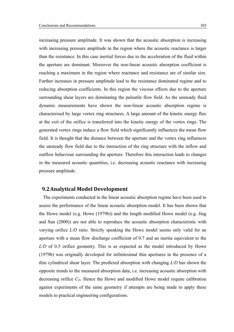
Conclusions and Recommendations 303
increasing pressure amplitude. It was shown that the acoustic absorption is increasing
with increasing pressure amplitude in the region where the acoustic reactance is larger
than the resistance. In this case inertial forces due to the acceleration of the fluid within
the aperture are dominant. Moreover the non-linear acoustic absorption coefficient is
reaching a maximum in the region where reactance and resistance are of similar size.
Further increases in pressure amplitude lead to the resistance dominated regime and to
reducing absorption coefficients. In this region the viscous effects due to the aperture
surrounding shear layers are dominating the pulsatile flow field. As the unsteady fluid
dynamic measurements have shown the non-linear acoustic absorption regime is
characterised by large vortex ring structures. A large amount of the kinetic energy flux
at the exit of the orifice is transferred into the kinetic energy of the vortex rings. The
generated vortex rings induce a flow field which significantly influences the mean flow
field. It is thought that the distance between the aperture and the vortex ring influences
the unsteady flow field due to the interaction of the ring structure with the inflow and
outflow behaviour surrounding the aperture. Therefore this interaction leads to changes
in the measured acoustic quantities, i.e. decreasing acoustic reactance with increasing
pressure amplitude.
9.2 Analytical Model Development The experiments conducted in the linear acoustic absorption regime have been used to
assess the performance of the linear acoustic absorption model. It has been shown that
the Howe model (e.g. Howe (1979b)) and the length modified Howe model (e.g. Jing
and Sun (2000)) are not able to reproduce the acoustic absorption characteristic with
varying orifice L/D ratio. Strictly speaking the Howe model seems only valid for an
aperture with a mean flow discharge coefficient of 0.7 and an inertia equivalent to the
L/D of 0.5 orifice geometry. This is as expected as the model introduced by Howe
(1979b) was originally developed for infinitesimal thin apertures in the presence of a
thin cylindrical shear layer. The predicted absorption with changing L/D has shown the
opposite trends to the measured absorption data, i.e. increasing acoustic absorption with
decreasing orifice CD. Hence the Howe and modified Howe model require calibration
against experiments of the same geometry if attempts are being made to apply these
models to practical engineering configurations.

Conclusions and Recommendations 304
A better model to use is the linear solution to the unsteady momentum equation as
proposed by Bellucci et. al. (2004). It was shown that it is sufficient to use the mean
discharge coefficients in the linear regime to predict the absorption characteristic with
changing L/D ratio. Nevertheless the model still needs empirical length correction terms
for an accurate prediction of the acoustic absorption over a wide Strouhal number range.
It has been shown that the use of constant loss coefficients and length corrections in the
linear acoustic absorption model is valid as long as there are no large scale structures
developing (as is the case for self-excited jet instabilities). The Bellucci et. al. linear
acoustic absorption model showed excellent agreement with all experimental validation
data for L/D ratios up to five. For increasing hole length the modelling techniques
showed increasing discrepancies with the experimental data.
The model proposed by Bellucci et. al. (2004) can also be used in the non-linear
absorption regime. A function based on the ratio of unsteady velocity amplitude to mean
velocity controls the transition from linear to non-linear acoustic absorption. However
as the experimental results have shown the transition to non-linear acoustic absorption
occurs at a smaller ratio of velocity amplitude to mean velocity through the aperture
than assumed by the current model. In the non-linear regime the mentioned interactions
between large scale vortex rings and the pulsatile flow field cause changes in loss
coefficients and length corrections which are required as an input to the model. Thus the
input parameters to the model are no longer constant but functions of pressure
amplitude and frequencies. Currently empirical curve fits could be used to estimate the
change in length correction and loss coefficients with varying pressure and frequency.
9.3 Engine Representative Damper Configurations The analytical model proposed by Bellucci et. al. has been incorporated into a set of
design tools for acoustic dampers applied to gas turbine combustion systems. Using this
approach it is possible to define the geometric parameters of a damper, tune it to the
relevant frequencies within the gas turbine combustion system design envelope and
assess the generated acoustic absorption as well as the risk of hot gas ingestion for
increased pressure amplitude. The acoustic damper performance has also been assessed
in a more representative geometry. In this way a test section representative of a single

Conclusions and Recommendations 305
sector of a full annular combustion system has been studied. This includes exposure of
an acoustic damper to the complex swirling flow field generated by a modern lean burn
fuel injector has been investigated. The developed acoustic modelling method based on
Bellucci et. al. (2004) was used to predict the acoustic absorption of the damper. It was
shown that the model and the experiment were in good agreement. The model does not
take any swirling or cross-flow influences into account. Hence the influence of the
complex swirling flow field and cross flow field had no significant effect upon the bulk
absorption characteristic of the damper. The acoustic energy loss is not only a function
of the aperture geometry but also a function of the unsteady pressure drop across the
damping skin. Hence maximising the unsteady pressure drop for a given aperture
geometry increases the acoustic losses. Therefore the loss of the investigated broadband
liner could be increased if the cavity volume between the perforated liners acts as a
plenum (i.e. pressure amplitude equal to zero). However in this case the size of the
cavity volume would be too large to fit into the design envelope of an aero-engine gas
turbine. Hence a more efficient way to increase the absorption of double skin acoustic
dampers is to tune the cavity such that it is in resonance (e.g. as it is found with
Helmholtz resonators). In this case the unsteady pressure difference across the damping
skin can be maximised in the vicinity of the resonance frequency.
As already mentioned the main objective was to understand how much acoustic
absorption is available within a conventional combustion system. Within the linear
acoustic absorption regime this can be answered using the developed modelling
techniques. Most of the combustor wall cooling apertures operate within the quasi-
steady regime. In this case the developed quasi-steady acoustic loss assumption based
on the mean mass flow and mean pressure drop quantities can be used. Finally the
developed impedance methodology can be utilised to superimpose the cooling
geometries, damping geometries and fuel injector impedances to estimate the total
acoustic loss of a combustion system. Ultimately the linear acoustic absorption model
should be used within acoustic network models to improve the accuracy of the full
annular combustion system stability predictions.
Conclusions and Recommendations 306
9.4 Recommendations The used linear acoustic model has shown increasing discrepancies with the
experimental data for aperture geometries longer than L/D of five. For long apertures
with orifice length larger L/D of two the flow field reattaches within the orifice leading
to the formation of a boundary layer inside the orifice. Hence the associated loss
coefficients are a representation of inflow losses, viscous losses due to the boundary
layer and outflow losses. Two possible short term solutions have been shown within the
work: (i) only use the measured mean flow discharge coefficient without the unsteady
viscosity model or (ii) use the mean flow discharge coefficient for an L/D of two orifice
together with the unsteady viscosity model. The latter option showed the better
agreement with the experiment. However, this behaviour should be further investigated
by utilising flow field simulations (e.g. Mendez and Eldredge (2009) or Gunasekaran
and McGuirk (2011)) or measurements inside a long L/D aperture to develop
representative unsteady viscosity models as well as getting a better understanding of the
inflow and outflow loss coefficient. The developed unsteady flow field methodology
could be used to identify the relevant flow field phenomena.
In this study all the apertures where investigated during inflow conditions without the
influence of cross flow. It is known that the mean flow discharge coefficient is
significantly affected by cross flow conditions on the inflow side to the aperture. In gas
turbine combustors this has technical relevance as many apertures are fed from the
surrounding annulus with cross-flow streams across the aperture on the inflow side.
Hence the linear analytical modelling technique and its validity should be assessed
against experiments with cross flow on the upstream side of the orifice.
The non-linear modelling technique as well as the transition from linear to non-linear
acoustic absorption remains challenging. In this case vortex ring structures interact with
the unsteady flow field which therefore affect the acoustic absorption characteristic.
More detailed unsteady flow simulations using CFD or measurements in conjunction
with the developed unsteady flow field methodology should be utilised to improve the
simplified analytical non-linear modelling techniques.
Similar analytical modelling techniques applied to circular orifices should also be
applied to fuel injector geometries. Accurate impedance models of the fuel injectors are

Conclusions and Recommendations 307
important for an accurate application of acoustic network models for the stability
prediction of a gas turbine combustion system. Moreover the acoustic impedance of the
fuel injector could also be studied with the aim of reducing the unsteady velocity field
through the fuel injector relative to an incident pressure amplitude. This may help to
reduce the onset of thermo-acoustic instabilities at source.

References 308
References
Åbom, M. & Bodén, H. 1988, "Error analysis of two‐microphone measurements in ducts with flow", The Journal of the Acoustical Society of America, vol. 83, pp. 2429-2438.
ACARE 2011, “Flightpath 2050 Europe's vision for aviation”.
ACARE 2001, “European aeronautics: A vision for 2020”.
Adrian, R.J. 2005, "Twenty years of particle image velocimetry", Experiments in Flu-ids, vol. 39, no. 2, pp. 159-169.
Adrian, R.J. 1991, "Particle-imaging techniques for experimental fluid mechan-ics", Annual Review of Fluid Mechanics, vol. 23, no. 1, pp. 261-304.
Adrian, R.J., Christensen, K.T. & Liu, Z.C. 2000, "Analysis and interpretation of instan-taneous turbulent velocity fields", Experiments in Fluids, vol. 29, no. 3, pp. 275-290.
Andreini, A., Bianchini, C., Facchini, B., Simonetti, F. & Peschiulli, A. 2011, "Assess-ment of numerical tools for the evaluation of the acoustic impedance of multi-perforated plates", ASME Turbo Expo, GT2011-46303, June 6-10, Vancouver, Canada.
Atig, M., Dalmont, J.P. & Gilbert, J. 2004, "Termination impedance of open-ended cy-lindrical tubes at high sound pressure level", Comptes Rendus Mécanique, vol. 332, no. 4, pp. 299-304.
Aydemir, E., Worth, N.A. & Dawson, J.R. 2012, "The formation of vortex rings in a strongly forced round jet", Experiments in Fluids, vol. 52, pp. 729-742.
Barker, A., Carrotte, J. & Denman, P. 2005, "Analysis of hot-wire anemometry data in an acoustically excited turbulent flow field", Experiments in Fluids, vol. 39, no. 6, pp. 1061-1070.
Barker, A. & Carrotte, J.F. 2006, “Factors limiting the performance of Helmholtz reso-nators in gas turbine combustors”, TT06R04, Loughborough University.
Batchelor, G.K. 2000, “An introduction to fluid dynamics”, Cambridge University Press.
Bechert, D., Michel, U. & Pfizenmaier, E. 1977, "Experiments on the transmission of sound through jets", American Institute of Aeronautics and Astronautics, 4th Aeroa-coustics Conference, Atlanta, Georgia.
Bechert, D. 1980, "Sound absorption caused by vorticity shedding, demonstrated with a jet flow", Journal of Sound and Vibration, vol. 70, no. 3, pp. 389-405.

References 309
Bellucci, V., Flohr, P. & Paschereit, C.O. 2004b, "Numerical and experimental study of
acoustic damping generated by perforated screens", AIAA Journal, vol. 42, no. 8, pp. 1543-1549.
Bellucci, V., Flohr, P., Paschereit, C.O. & Magni, F. 2004, "On the use of Helmholtz resonators for damping acoustic pulsations in industrial gas turbines", Journal of engineering for gas turbines and power, vol. 126, pp. 271-275.
Bellucci, V., Schuermans, B., Nowak, D., Flohr, P. & Paschereit, C.O. 2005, "Thermo-acoustic modeling of a gas turbine combustor equipped with acoustic damp-ers", Journal of turbomachinery, vol. 127, pp. 372-379.
Beranek, L.L. 1954, “Acoustics”, McGraw-Hill.
Berkooz, G., Holmes, P. & Lumley, J.L. 1993, "The proper orthogonal decomposition in the analysis of turbulent flows", Annual Review of Fluid Mechanics, vol. 25, no. 1, pp. 539-575.
Bernero, S. & Fiedler, H.E. 2000, "Application of particle image velocimetry and prop-er orthogonal decomposition to the study of a jet in a counterflow", Experiments in Fluids, vol. 29, pp. 274-281.
Betts, J.F. 2000, “Experiments and impedance modeling of liners Including the effect of bias flow”, Virginia Polytechnic Institute and State University.
Blokhintsev, D. 1956, "Acoustics of a Nonhomogeneous Moving Medium", NACA, Technical Memorandum 1399.
Bodén, H. & Åbom, M. 1986, "Influence of errors on the two‐microphone method for measuring acoustic properties in ducts", The Journal of the Acoustical Society of America, vol. 79, pp. 541-549.
Bonnell, J.M., Marshall, R.L. & Riecke, G.T. 1971, "Combustion instability in turbojet and turbofan augmentors", AIAA/SAE 7th Propulsion Joint Specialist Conference, June 14-18.
Bothien, M.R., Noiray, N. & Schuermans, B. 2012, "A Novel Damping Device for Broadband Attenuation of Low-Frequency Combustion Pulsations in Gas Tur-bines", ASME Turbo Expo, GT2012-68873, June 11-15, Copenhagen, Denmark.
Brown, G.B. 1935, "On vortex motion in gaseous jets and the origin of their sensitivity to sound", Proceedings of the Physical Society, vol. 47, pp. 703-732.
Candel, S. 2002, "Combustion dynamics and control: progress and challeng-es", Proceedings of the combustion institute, vol. 29, no. 1, pp. 1-28.
Chanaud, R. 1994, "Effects of geometry on the resonance frequency of Helmholtz reso-nators", Journal of Sound and Vibration, vol. 178, no. 3, pp. 337-348.
Chatterjee, A. 2000, "An introduction to the proper orthogonal decomposition", Current science, vol. 78, no. 7, pp. 808-817.

References 310
Chu, B.T. 1965, "On the energy transfer to small disturbances in fluid flow (Part
I)", Acta Mechanica, vol. 1, no. 3, pp. 215-234.
Coats, C. 1996, "Coherent structures in combustion", Progress in Energy and Combus-tion Science, vol. 22, no. 5, pp. 427-509.
Cole-Parmer 2009, “Precision Gas Flow Controller Operating Manual”.
Crow, S.C. & Champagne, F.H. 1971, "Orderly structure in jet turbulence", Journal of Fluid Mechanics, vol. 48, no. 3, pp. 547-591.
Culick, F. 2006, “Unsteady motions in combustion chambers for propulsion systems”, AGARD, RTO-AG-AVT-039.
Cummings, A. 1987, "The response of a resonator under a turbulent boundary layer to a high amplitude non-harmonic sound field", Journal of Sound and Vibration, vol. 115, no. 2, pp. 321-328.
Cummings, A. 1986, "Transient and multiple frequency sound transmission through perforated plates at high amplitude", The Journal of the Acoustical Society of America, vol. 79, pp. 942.
Cummings, A. & Eversman, W. 1983, "High amplitude acoustic transmission through duct terminations: theory", Journal of Sound and Vibration, vol. 91, no. 4, pp. 503-518.
de Bedout, J., Franchek, M., Bernhard, R. & Mongeau, L. 1997, "Adaptive passive noise control with self-tuning Helmholtz resonators", Journal of Sound and Vibra-tion, vol. 202, no. 1, pp. 109-123.
Dean, P. & Tester, B. 1975, "Duct wall impedance control as an advanced concept for acoustic suppression", NASA Contractor Report CR-134998.
Didden, N. 1979, "On the formation of vortex rings: rolling-up and production of circu-lation", Zeitschrift für Angewandte Mathematik und Physik (ZAMP), vol. 30, no. 1, pp. 101-116.
Disselhorst, J. & Wijngaarden, L.V. 1980, "Flow in the exit of open pipes during acous-tic resonance", Journal of Fluid Mechanics, vol. 99, no. 02, pp. 293-319.
Dodds, W. 2005, "Twin annular premixing swirler (TAPS) combustor", The Roaring 20th Aviation Noise & Air Quality Symposium.
Dodds, W. 2002, "Engine and aircraft technologies to reduce emissions", UC Technolo-gy Transfer Symposium―Dreams of Flight.
Douglas, J.F., Gasiorek, J.M., Swaffield, J.A. & Jack, L.B. 2005, “Fluid Mechanics”, 5th edition, Pearson Prentice Hall.
Dowling, A.P. 2003, "The challenges of lean premixed combustion", Proceedings of the International Gas Turbine Congress, Tokyo, November 2-7.

References 311
Dowling, A.P. & Morgans, A.S. 2005, "Feedback control of combustion oscilla-
tions", Annual Review of Fluid Mechanics, vol. 37, pp. 151-182.
Dowling, A.P. & Stow, S.R. 2003, "Acoustic analysis of gas turbine combus-tors", Journal of Propulsion and Power, vol. 19, no. 5, pp. 751-764.
Dowling, A. & Hubbard, S. 2000, "Instability in lean premixed combus-tors", Proceedings of the Institution of Mechanical Engineers, Part A: Journal of Power and Energy, vol. 214, no. 4, pp. 317-332.
Dowling, A. & Hughes, I. 1992, "Sound absorption by a screen with a regular array of slits", Journal of Sound and Vibration, vol. 156, no. 3, pp. 387-405.
Dunham, D. 2011, “Unsteady fluid mechanics of annular swirling shear layers”, Lough-borough University.
Eckstein, J. 2004, “On the mechanisms of combustion driven low-frequency oscillations in aero-engines”, Technische Universität München.
Eckstein, J., Freitag, E., Hirsch, C. & Sattelmayer, T. 2004, "Experimental study on the role of entropy waves in low-frequency oscillations for a diffusion burner", ASME Turbo Expo, GT2004-54163, June 14-17, Vienna, Austria.
Eldredge, J.D. 2004, "On the interaction of higher duct modes with a perforated liner system with bias flow", Journal of Fluid Mechanics, vol. 510, no. 1, pp. 303-331.
Eldredge, J.D., Bodony, D.J. & Shoeybi, M. 2007, "Numerical investigation of the acoustic behavior of a multi-perforated liner", Proceedings of the 13th AIAA/CEAS Aeroacoustics Conference, AIAA Paper 2007-3683, 21-23 May.
Eldredge, J.D. & Dowling, A.P. 2003, "The absorption of axial acoustic waves by a perforated liner with bias flow", Journal of Fluid Mechanics, vol. 485, no. 25, pp. 307-335.
Forster, S. & Michel, U. 2003, "Experimental investigation of the dissipation of acous-tic energy in perforated walls with bias flow", Combustion and Noise Control Cranfield University Press.
Freymuth, P. 1966, "On transition in a separated laminar boundary layer", Journal of Fluid Mechanics, vol. 25, no. 4, pp. 683-704.
Garrison, G.D., Russel, P.L. & Stettler, J. 1972, “Investigation of damping methods for augmentor combustion instability”, DTIC Document, AFAPL-TR-7284.
Gharib, M., Rambod, E. & Shariff, K. 1998, "A universal time scale for vortex ring formation", Journal of Fluid Mechanics, vol. 360, no. 1, pp. 121-140.
Glezer, A. 1988, "The formation of vortex rings", Physics of Fluids, vol. 31, no. 12, pp. 3532-3542.

References 312
Graftieaux, L., Michard, M. & Grosjean, N. 2001, "Combining PIV, POD and vortex
identification algorithms for the study of unsteady turbulent swirling flows", Meas-urement Science and technology, vol. 12, pp. 1422-1429.
Gritsch, M., Schulz, A. & Wittig, S. 1998, "Discharge coefficient measurements of film-cooling holes with expanded exits", Journal of Turbomachinery, vol. 120, pp. 557-563.
Gunasekaran, B. & McGuirk, J.J. 2011, "Mildly-Compressible Pressure-Based CFD Methodology for Acoustic Propagation and Absorption Prediction", ASME Turbo Expo, GT2011-45316, June 6-10, Vancouver, Canada.
Gysling, D.L., Copeland, G.S., McCormick, D.C. & Proscia, W.M. 2000, "Combustion system damping augmentation with Helmholtz resonators", Journal of Engineering for Gas Turbines and Power, vol. 122, pp. 269-274.
Hafsteinsson, H., Burak, M., Eriksson, L.E. & Billson, M. 2010, "Experimental and numerical investigation of a novel acoustic liner concept", 16th AIAA/CEAS Aeroa-coustics Conference, AIAA 2010-3847, 7-9 June.
Hart, R. & McClure, F. 1965, "Theory of acoustic instability in solid-propellant rocket combustion", Symposium (International) on Combustion , vol. 10, no. 1, pp. 1047-1065.
Hay, N., Henshall, S.E. & Manning, A. 1994, "Discharge coefficients of holes angled to the flow direction", Journal of Turbomachinery, vol. 116, pp. 92-96.
Hay, N. & Spencer, A. 1992, "Discharge coefficients of cooling holes with radiused and chamfered inlets", Journal of Turbomachinery, vol. 114, pp. 701-706.
Heavens, S.N. 1980, "Visualization of the acoustic excitation of a subsonic jet", Journal of Fluid Mechanics, vol. 100, pp. 185-192.
Hersh, A.S. & Rogers, T. 1976, “Fluid mechanical model of the acoustic impedance of small orifices”, NASA Contractor Report, CR-2682.
Hersh, A.S., Walker, B.E. & Celano, J.W. 1999, "Semi-empirical Helmholtz resonator impedance model", AIAA/CEAS Aeroacoustics Conference and Exhibit, AIAA-99-1825.
Heuwinkel, C., Enghardt, L. & Röhle, I. 2007, "Experimental investigation of the acoustic damping of perforated liners with bias flow", AIAA 13th Aeroacoustics Conference, AIAA 2007-3525, 21-23 May.
Higgins, B. 1802, "On the sound produced by a current of hydrogen gas passing through a tube", Journal of Natural Philosophy Chemistry and the Arts, vol. 1, p. 129.
Hollis, D. 2004, “Particle image velocimetry in gas turbine combustor flow fields”, Loughborough University.

References 313
Holmes, P., Lumley, J.L. & Berkooz, G. 1998, “Turbulence, coherent structures, dy-
namical systems and symmetry”, Cambridge University Press.
Howe, M.S. 1979a, "Attenuation of sound in a low Mach number nozzle flow", Journal of Fluid Mechanics, vol. 91, no. 2, pp. 209-229.
Howe, M. 1979b, "On the theory of unsteady high Reynolds number flow through a circular aperture", Proceedings of the Royal Society of London A. Mathematical and Physical Sciences, vol. 366, pp. 205-223.
Huang, Y. & Yang, V. 2009, "Dynamics and stability of lean-premixed swirl-stabilized combustion", Progress in energy and combustion science, vol. 35, no. 4, pp. 293-364.
Hughes, I. & Dowling, A. 1990, "The absorption of sound by perforated lin-ings", Journal of Fluid Mechanics, vol. 218, pp. 299-335.
Hussain, A.K.M.F. & Zaman, K.B.M.Q. 1981, "The ‘preferred mode’of the axisymmet-ric jet", Journal of Fluid Mechanics, vol. 110, no. 1, pp. 39-71.
ICAO 2010, “Environmental Report”.
Illingworth, S.J. & Morgans, A.S. 2010, "Adaptive feedback control of combustion in-stability in annular combustors", Combustion Science and Technology, vol. 182, no. 2, pp. 143-164.
Ingard, U. 1970, "Nonlinear distortion of sound transmitted through an orifice", The Journal of the Acoustical Society of America, vol. 48, no. 1, pp. 32-33.
Ingard, U. 1968, "Absorption characteristics of nonlinear acoustic resonators", The Journal of the Acoustical Society of America, vol. 44, no. 4, pp. 1155-1156.
Ingard, U. 1953, "On the theory and design of acoustic resonators", The Journal of the Acoustical Society of America, vol. 25, no. 6, pp. 1037-1061.
Ingard, U. & Ising, H. 1967, "Acoustic nonlineartry of an orifice", The Journal of the Acoustical Society of America, vol. 42, no. 1, pp. 6-17.
Ingard, U. & Labate, S. 1950, "Acoustic circulation effects and the nonlinear impedance of orifices", The Journal of the Acoustical Society of America, vol. 22, pp. 211-218.
Jabbal, M., Wu, J. & Zhong, S. 2006, "The performance of round synthetic jets in qui-escent flow", Aeronautical Journal, vol. 110, no. 1108, pp. 385-393.
Jeong, J. & Hussain, F. 1995, "On the identification of a vortex", Journal of Fluid Me-chanics, vol. 285, no. 1, pp. 69-94.
Jing, X. & Sun, X. 2002, "Sound-excited flow and acoustic nonlinearity at an ori-fice", Physics of Fluids, vol. 14, no. 1, pp. 268-276.
Jing, X. & Sun, X. 2000, "Effect of plate thickness on impedance of perforated plates with bias flow", AIAA Journal, vol. 38, no. 9, pp. 1573-1578.

References 314
Jing, X. & Sun, X. 1999, "Experimental investigations of perforated liners with bias
flow", The Journal of the Acoustical Society of America, vol. 106, no. 5, pp. 2436-2441.
Johnston, J.P. & Schmidt, W.E. 1978, "Measurement of acoustic reflection from an ob-struction in a pipe with flow", The Journal of the Acoustical Society of America, vol. 63, pp. 1455-1460.
Kato, S., Fujimori, T., Dowling, A. & Kobayashi, H. 2005, "Effect of heat release dis-tribution on combustion oscillation", Proceedings of the Combustion Institute, vol. 30, no. 2, pp. 1799-1806.
Kaufmann, P., Krebs, W., Valdes, R. & Wever, U. 2008, "3D thermoacoustic properties of single can and multi can combustor configurations", ASME Turbo Expo, GT2008-50755, June 9-13, Berlin, Germany.
Keane, R.D. & Adrian, R.J. 1990, "Optimization of particle image velocimeters. I. Double pulsed systems", Measurement Science and Technology, vol. 1, pp. 1202-1215.
Keller, J.J. & Zauner, E. 1995, "On the use of Helmholtz resonators as sound attenua-tors", Zeitschrift für Angewandte Mathematik und Physik (ZAMP), vol. 46, no. 3, pp. 297-327.
Kinsler, L.E., Frey, A.R., Coppens, A.B. & Sanders, J.V. 1999, “Fundamentals of acoustics”, 4th edition, Wiley-VCH.
Klinger, H., Lazik, W. & Wunderlich, T. 2008, "The engine 3E core engine", ASME Turbo EXPO, GT2008-50679, June 9-13, Berlin, Germany.
Ko, S.H. 1972, "Sound attenuation in acoustically lined circular ducts in the presence of uniform flow and shear flow", Journal of Sound and Vibration, vol. 22, no. 2, pp. 193-210.
Kolár, V. 2007, "Vortex identification: New requirements and limita-tions", International Journal of Heat and Fluid Flow, vol. 28, no. 4, pp. 638-652.
Kostas, J., Soria, J. & Chong, M.S. 2005, "A comparison between snapshot POD analy-sis of PIV velocity and vorticity data", Experiments in Fluids, vol. 38, no. 2, pp. 146-160.
Krebs, W., Bethke, S., Lepers, J., Flohr, P., Prade, B., Johnson, C. & Sattinger, S. 2005, "Thermoacoustic design tools and passive control: Siemens power generation ap-proaches", Combustion Instabilities in Gas Turbine Engines Operational Experi-ence, Fundamental Mechanisms and Modeling, editors T.C. Lieuwen & V. Yang, AIAA.
Krueger, P.S., Dabiri, J.O. & Gharib, M. 2006, "The formation number of vortex rings formed in uniform background co-flow", Journal of Fluid Mechanics, vol. 556, no. 1, pp. 147-166.

References 315
Lahiri, C., Enghardt, L., Bake, F., Sadig, S. & Gerendas, M. 2011, "Establishment of a
high quality database for the acoustic modeling of perforated liners", Journal of Engineering for Gas Turbines and Power, vol. 133, pp. 091503.
Langhorne, P. 1988, "Reheat buzz: an acoustically coupled combustion instability. Part 1. Experiment", Journal of Fluid Mechanics, vol. 193, no. 1, pp. 417-443.
Laudien, E., Pongratz, R., Pierro, R. & Preclik, D. 1995, "Experimental procedures aid-ing the design of acoustic cavities", Liquid Rocket Engine Combustion Instability, editors V. Yang & W.E. Anderson, AIAA.
LaVision 2011, “Product Manual Darwin Duo”, LaVision.
LaVision 2007, “Flow master product manual”, La Vision.
Lawn, C. 2000, "The thermo-acoustic response of a premixed swirl burn-er", Proceedings of the Institution of Mechanical Engineers, Part A: Journal of Power and Energy, vol. 214, no. 4, pp. 333-354.
Lazik, W., Doerr, T., Bake, S., von der Bank, R. & Rackwitz, L. 2008, "Development of lean-burn Low-NOx Combustion Technology at Rolls-Royce Deutschland", ASME Turbo EXPO, GT2008-51115, June 9-13, Berlin, Germany.
Lebedeva, I.V., Grushin, A.E. & Kravtsov, Y.U. 2005, "Experimental study of aeroa-coustic characteristics of screens with an orifice", International Journal of Aeroa-coustics, vol. 4, no. 3, pp. 345-352.
Lee, D.S., Fahey, D.W., Forster, P.M., Newton, P.J., Wit, R.C.N., Lim, L.L., Owen, B. & Sausen, R. 2009, "Aviation and global climate change in the 21st century", At-mospheric Environment, vol. 43, no. 22-23, pp. 3520-3537.
Lee, S.H., Ih, J.G. & Peat, K.S. 2007, "A model of acoustic impedance of perforated plates with bias flow considering the interaction effect", Journal of Sound and Vi-bration, vol. 303, no. 3, pp. 741-752.
Lefebvre, A.H. & Ballal, D.R. 2010, “Gas turbine combustion alternative fuels and emissions”, 3rd edition, CRC Press.
Lewis, J.S. & Niedzwiecki, R.W. 1999, "Aircraft technology and its relation to emis-sions", Avaiation and the Global Atmosphere, Intergovernmental Panel on Climate Change, editors J.E. Penner, D.H. Lister, D.J. Griggs, D.J. Dokken & M. MacFar-land, Cambridge University Press, Oxford.
Lichtarowicz, A., Duggins, R.K. & Markland, E. 1965, "Discharge coefficients for in-compressible non‐cavitating flow through long orifices", Journal of Mechanical Engineering Science, vol. 7, no. 2, pp. 210-219.
Lieuwen, T.C. 1999, “Investigation of combustion instability mechanisms in premixed gas turbines”, Georgia Institute of Technology.

References 316
Lieuwen, T.C. & Zinn, B.T. 1998, "The role of equivalence ratio oscillations in driving
combustion instabilities in low NOX gas turbines", Symposium (International) on Combustion, vol. 27 , no. 2, pp. 1809-1816.
Lim, T.T., New, T.H. & Luo, S.C. 2001, "On the development of large-scale structures of a jet normal to a cross flow", Physics of Fluids, vol. 13, pp. 770-775.
Lörstad, D., Pettersson, J. & Lindholm, A. 2009, "Emission reduction and cooling im-provements due to the introduction of passive acoustic damping in an existing SGT-800 combustor", ASME Turbo Expo, GT2009-59313, June 8-12, Orlando, Florida.
Lucas, M.J., Noreen, R., Sutherland, L.C., Coleman, J.E. & Junger, M.C. 1997, “Handbook of the acoustic characteristics of turbomachinery cavi-ties”, ASME Press.
Luong, T., Howe, M.S. & McGowan, R.S. 2005, "On the Rayleigh conductivity of a bias-flow aperture", Journal of Fluids and Structures, vol. 21, no. 8, pp. 769-778.
Lynn, P.A. 1989, “Introduction to the Analysis and Processing of Signals”, Hemisphere Publishing Corporation.
Macquisten, M.A., Holt, A., Whiteman, M., Moran, A.J. & Rupp, J. 2006, "Passive damper LP tests for controlling combustion instability", ASME Turbo Expo, GT2006-90874, May 8-11, Barcelona, Spain.
Maxworthy, T. 1977, "Some experimental studies of vortex rings", Journal of Fluid Mechanics, vol. 81, no. 3, pp. 465-495.
Melling, T.H. 1973, "The acoustic impedance of perforates at medium and high sound pressure levels", Journal of Sound and Vibration, vol. 29, no. 1, pp. 1-65.
Mendez, S. & Eldredge, J. 2009, "Acoustic modeling of perforated plates with bias flow for Large-Eddy Simulations", Journal of Computational Physics, vol. 228, no. 13, pp. 4757-4772.
Michalke, A. 1972, "The instability of free shear layers", Progress in Aerospace Scienc-es, vol. 12, pp. 213-216.
Midgley, K. 2005, “An isothermal experimental study of the unsteady fluid mechanics of gas turbine fuel injector flow fields”, Loughborough University.
Moler, C.B. 2004, “Numerical computing with MATLAB”, Society for Industrial Mathematics.
Mongia, H.C., Held, T.J., Hsiao, G.C. & Pandalai, R.P. 2003, "Challenges and progress in controlling dynamics in gas turbine combustors", Journal of Propulsion and Power, vol. 19, no. 5, pp. 822-829.
Montgomery, D.C. & Runger, G.C. 1994, “Applied statistics and probability for engi-neers”, Wiley.

References 317
Moran, A.J., Steele, D. & Dowling, A.P. 2001, “Active control of combustion and its
applications”, DTIC Document, ADP011145.
Morfey, C.L. 1971, "Acoustic energy in non-uniform flows", Journal of Sound and Vi-bration, vol. 14, no. 2, pp. 159-170.
Morris, A.S. 2001, “Measurement and instrumentation principles”, Butterworth-Heinemann.
Oertel, H. & Böhle, M. 2002, “Strömungsmechanik: Grundlagen-Grundgleichungen-Lösungsmethoden-Softwarebeispiele”, Vieweg Verlag.
Paschereit, C.O., Gutmark, E. & Weisenstein, W. 1999, "Control of combustion driven oscillations by equivalence ratio modulations", ASME Turbo Expo, 99-GT-118, June 7-10, Indianapolis, IN.
Paschereit, C.O., Schuermans, B., Polifke, W. & Mattson, O. 2002, "Measurement of transfer matrices and source terms of premixed flames", Journal of Engineering for Gas Turbines and Power, vol. 124, pp. 239-247.
Patte-Rouland, B., Lalizel, G., Moreau, J. & Rouland, E. 2001, "Flow analysis of an annular jet by particle image velocimetry and proper orthogonal decomposi-tion", Measurement Science and Technology, vol. 12, pp. 1404-1412.
Peacock, G. 2011, “Fuel injector impedance measurements”.
Poinsot, T., Le Chatelier, C., Candel, S. & Esposito, E. 1986, "Experimental determina-tion of the reflection coefficient of a premixed flame in a duct", Journal of Sound and Vibration, vol. 107, no. 2, pp. 265-278.
Poinsot, T.J., Trouve, A.C., Veynante, D.P., Candel, S.M. & Esposito, E.J. 1987, "Vor-tex-driven acoustically coupled combustion instabilities", Journal of Fluid Me-chanics, vol. 177, no. 1, pp. 265-292.
Pope, S.B. 2000, “Turbulent flows”, Cambridge University Press.
Prather, M., Sausen, R., Grossman, A.S., Haywood, J.M., Rind, D. & Subbaraya, B.H. 1999, "Potential climate change from aviation", Aviation and the Global Atmos-phere, Intergovernmental Panel on Climate Change, editors J.E. Penner, D.H. Lis-ter, D.J. Griggs, D.J. Dokken & M. McFarland, Cambridge University Press.
Putnam, A.A. 1971, “Combustion-driven oscillations in industry”, Elsevier New York.
Raffel, M., Willert, C.E., Wereley, S. & Kompenhans, J. 2007, “Particle image veloci-metry: a practical guide”, 2nd edition, Springer Verlag.
Rayleigh, J.W.S. 1896, “The Theory of Sound, Vol. 2”, 2nd edition, 1945, Dover, New York.
Richards, G.A., Straub, D.L. & Robey, E.H. 2003, "Passive control of combustion dy-namics in stationary gas turbines", Journal of Propulsion and Power, vol. 19, no. 5, pp. 795-810.

References 318
Rijke, P.L. 1859, "LXXI. Notice of a new method of causing a vibration of the air con-
tained in a tube open at both ends", The London, Edinburgh, and Dublin Philo-sophical Magazine and Journal of Science, vol. 17, no. 116, pp. 419-422.
Riley, A.J., Park, S., Dowling, A.P., Evesque, S. & Annaswamy, A.M. 2003, "Adaptive closed-loop control on an atmospheric gaseous lean-premixed combustor", ASME Turbo Expo, GT2003-38418, June 16–19, Atlanta, Georgia.
Robinson, M.D. 2009, “Unsteady inlet condition generation for large eddy simulation CFD using particle image velocimetry”, Loughborough University.
Robinson, M.D. 2006, “Xact - User's guide”, Loughborough University.
Rogers, D.E. & Marble, F.E. 1956, "A mechanism for high-frequency oscillation in ramjet combustors and afterburners", Jet Propulsion, vol. 26, no. 6, pp. 456-462.
Rolls-Royce 2010, “Powering a better world Health, safety and environment report”.
Rolls-Royce 2005, “The jet engine”.
Rouse, H. & Abul-Fetouh, A. 1950, "Characteristics of irrotational flow through axially symmetric orifices", Journal of Applied Mechanics, vol. 17, no. 12, pp. 421-426.
Rowbury, D.A., Oldfield, M.L.G. & Lock, G.D. 2001, "Large-scale testing to validate the influence of external crossflow on the discharge coefficients of film cooling holes", Journal of Turbomachinery, vol. 123, pp. 593-600.
Rupp, J. & Carrotte, J.F. 2011, “Acoustic energy/velocity field interactions for circular holes”, Annual Review, Loughborough University.
Rupp, J., Carrotte, J.F. & Macquisten, M.A. 2012, "The use of perforated damping lin-ers in aero gas turbine combustion systems", Journal of engineering for gas tur-bines and power, vol. 134, no. 7, pp. 071502.
Rupp, J., Carrotte, J.F. & Spencer, A. 2010b, "Methodology to identify the unsteady flow field associated with the loss of acoustic energy in the vicinity of circular holes", ASME Turbo Expo, GT 2010-22178, June 14-18, Glasgow, UK.
Rupp, J., Carrotte, J.F. & Spencer, A. 2010, "Interaction between the acoustic pressure fluctuations and the unsteady flow field through circular holes", Journal of Engi-neering for Gas Turbines and Power, vol. 132, no. 6, pp. 061501.
Saffman, P.G. 1992, “Vortex dynamics”, Cambridge University Press.
Saffman, P.G. 1970, "The velocity of viscous vortex rings", Studies in Applied Mathe-matics, vol. 49, no. 4, pp. 371-380.
Salikuddin, M. & Brown, W. 1990, "Non-linear effects in finite amplitude wave propa-gation through orifice plate and perforated plate terminations", Journal of Sound and Vibration, vol. 139, no. 3, pp. 383-405.

References 319
Salikuddin, M., Syed, A. & Mungur, P. 1994, "Acoustic characteristics of perforated
sheets with throughflow in a high intensity noise environment", Journal of Sound and Vibration, vol. 169, no. 2, pp. 145-177.
Sattelmayer, T. 2003, "Influence of the combustor aerodynamics on combustion insta-bilities from equivalence ratio fluctuations", Journal of Engineering for Gas Tur-bines and Power, vol. 125, pp. 11-19.
Scarano, F. & Riethmuller, M. 2000, "Advances in iterative multigrid PIV image pro-cessing", Experiments in Fluids, vol. 29, pp. 51-60.
Scarinci, T. 2005, "Combustion instability and its passive control: Rolls-Royce aerode-rivative engine experience", Combustion Instabilities in Gas Turbine Engines Op-erational Experience, Fundamental Mechanisms and Modeling, editors T.C. Lieu-wen & V. Yang, AIAA.
Scarinci, T. & Halpin, J.L. 2000, "Industrial trent combustor - combustion noise charac-teristics", Journal of Engineering for Gas Turbines and Power, vol. 122, pp. 280-286.
Schoeneborn, P.R. 1975, "The interaction between a single particle and an oscillating fluid", International Journal of Multiphase Flow, vol. 2, pp. 307-317.
Schram, C. & Riethmuller, M.L. 2002, "Measurement of vortex ring characteristics dur-ing pairing in a forced subsonic air jet", Experiments in Fluids, vol. 33, no. 6, pp. 879-888.
Schram, C. & Riethmuller, M. 2001, "Vortex ring evolution in an impulsively started jet using digital particle image velocimetry and continuous wavelet analysis", Meas-urement Science and Technology, vol. 12, pp. 1413-1421.
Schuermans, B. 2003, “Modeling and control of thermoacoustic instabilities”, École Polytechnique Fédérale de Lausanne.
Schuermans, B., Guethe, F., Pennell, D., Guyot, D. & Paschereit, C.O. 2010, "Thermo-acoustic modeling of a gas turbine using transfer functions measured under full en-gine pressure", Journal of Engineering for Gas Turbines and Power, vol. 132, pp. 111503.
Selamet, A. & Lee, I. 2003, "Helmholtz resonator with extended neck", The Journal of the Acoustical Society of America, vol. 113, pp. 1975-1985.
Seo, S.H. & Kim, Y.H. 2005, "Silencer design by using array resonators for low-frequency band noise reduction", The Journal of the Acoustical Society of America, vol. 118, pp. 2332-2338.
Seybert, A. & Ross, D. 1977, "Experimental determination of acoustic properties using a two-microphone random-excitation technique", The Journal of the Acoustical So-ciety of America, vol. 61, no. 5, pp. 1362-1370.

References 320
Seybert, A. & Soenarko, B. 1981, "Error analysis of spectral estimates with application
to the measurement of acoustic parameters using random sound fields in ducts", The Journal of the Acoustical Society of America, vol. 69, pp. 1190-1199.
Siegel, D. & Plueddemann, A. 1991, "The motion of a solid sphere in an oscillating flow- An evaluation of remotely sensed Doppler velocity estimates in the sea", Journal of Atmospheric and Oceanic Technology, vol. 8, pp. 296-304.
Sirovich, L. 1987, "Turbulence and the dynamics of coherent structures. Part I: Coher-ent structures", Quarterly of Applied Mathematics, vol. 45, no. 3, pp. 561-571.
Steele, R.C., Cowell, L.H., Cannon, S.M. & Smith, C.E. 2000, "Passive control of com-bustion instability in lean premixed combustors", Journal of Engineering for Gas Turbines and Power, vol. 122, pp. 412-419.
Stow, S.R. & Dowling, A.P. 2003, "Modelling of circumferential modal coupling due to Helmholtz resonators", ASME Turbo Expo, GT 2003-38168, June 16-19, Atlanta, Georgia.
Sullivan, I.S., Niemela, J.J., Hershberger, R.E., Bolster, D. & Donnelly, R.J. 2008, "Dy-namics of thin vortex rings", Journal of Fluid Mechanics, vol. 609, no. 1, pp. 319-347.
Sun, X., Jing, X., Zhang, H. & Shi, Y. 2002, "Effect of grazing–bias flow interaction on acoustic impedance of perforated plates", Journal of Sound and Vibration, vol. 254, no. 3, pp. 557-573.
Tam, C.K.W., Ju, H., Jones, M., Watson, W. & Parrott, T. 2010, "A computational and experimental study of resonators in three dimensions", Journal of Sound and Vi-bration, vol. 329, no. 24, pp. 5164-5193.
Tam, C.K.W. & Kurbatskii, K.A. 2000, "Microfluid dynamics and acoustics of resonant liners", AIAA Journal, vol. 38, no. 8, pp. 1331-1339.
Tam, C.K.W., Kurbatskii, K.A., Ahuja, K. & Gaeta, R. 2001, "A numerical and experi-mental investigation of the dissipation mechanisms of resonant acoustic lin-ers", Journal of Sound and Vibration, vol. 245, no. 3, pp. 545-557.
Tang, S. 2005, "On Helmholtz resonators with tapered necks", Journal of Sound and Vibration, vol. 279, no. 3-5, pp. 1085-1096.
Testud, P., Aurégan, Y., Moussou, P. & Hirschberg, A. 2009, "The whistling potentiali-ty of an orifice in a confined flow using an energetic criterion", Journal of Sound and Vibration, vol. 325, no. 4, pp. 769-780.
Tondast-Navaei, A. 2005, “Acoustic particle image velocimetry - Development and applications”, The Open University.
Tran, N., Ducruix, S. & Schuller, T. 2008, "Passive control of the inlet acoustic bounda-ry of a swirled turbulent burner", ASME Turbo Expo, GT2008-50425, June 9-13, Berlin, Germany.

References 321
Umeh, C.O., Kammer, L.C. & Barbu, C. 2007, "Active combustion control by fuel forc-
ing at non-coherent frequencies", ASME Turbo Expo, GT2007-27637, May 14-17, Montreal, Canada.
Wendoloski, J.C. 1998, "Sound absorption by an orifice plate in a flow duct", The Jour-nal of the Acoustical Society of America, vol. 104, no. 1, pp. 122-132.
Westerweel, J. 1997, "Fundamentals of digital particle image veloci-metry", Measurement Science and Technology, vol. 8, pp. 1379-1392.
Westerweel, J. 1994, "Efficient detection of spurious vectors in particle image veloci-metry data", Experiments in Fluids, vol. 16, no. 3, pp. 236-247.
Whiffen, M.C. & Ahuja, K.K. 1983, "An improved schlieren system and some new re-sults on acoustically excited jets", Journal of Sound and Vibration, vol. 86, no. 1, pp. 99-105.
Wigley, G. 2008, “SAFEX fog generator particle size measurement”, Loughborough University.
Xu, M., Selamet, A. & Kim, H. 2010, "Dual Helmholtz resonator", Applied Acous-tics, vol. 71, no. 9, pp. 822-829.
Yang, V. & Anderson, W.E. 1995, “Liquid rocket engine combustion instabil-ity”, AIAA.
Yule, A.J. 1978, "Large-scale structure in the mixing layer of a round jet", Journal of Fluid Mechanics, vol. 89, no. 3, pp. 413-432.
Zhao, D., A'BARROW, C., Morgans, A.S. & Carrotte, J. 2009, "Acoustic Damping of a Helmholtz Resonator with an Oscillating Volume", AIAA journal, vol. 47, no. 7, pp. 1672-1679.
Zhao, D. & Morgans, A.S. 2009, "Tuned passive control of combustion instabilities using multiple Helmholtz resonators", Journal of Sound and Vibration, vol. 320, no. 4-5, pp. 744-757.
Zinn, B.T. 1970, "A theoretical study of non-linear damping by Helmholtz resona-tors", Journal of Sound and Vibration, vol. 13, no. 3, pp. 347-356.

Appendix
A. Orifice Geometry Definition
A.1 Orifice Geometries for Absorption Measurements The orifice plates investigated for the absorption experiments described in section
3.2.1 are specified in Table A.1. In the majority of cases the plates contain only one
aperture. However the plate with 3.3 mm orifice diameter contains multiple apertures to
increase the absorption of the orifice geometry which improved the measurement
accuracy. The diameters of the orifice were scaled to the relevant gas turbine engine
conditions (section 3.1). Where applicable the porosity and pitch-to-diameter ratio was
chosen to similar arrangements of gas turbine cooling geometries. For these values it is
assumed that the apertures within the gas turbine combustor cooling geometry are not
interacting (i.e. so allowing their absorption characteristic to be investigated in
isolation).
In total 17 orifice geometries have been investigated and their linear and non-linear
absorption has been measured. The length-to-diameter ratios L/D ranged from 0.5-10,
this range being relevant for the geometries found within gas turbine combustors. In
addition to cylindrical orifice plates various alternative orifice geometries where
investigated to enable an assessment on the effect of aperture geometry on linear and
non-linear absorption. Table A.2 shows schematics of the orifice shapes investigated in
this work. In general the shapes have been designed with the aim of showing significant
differences to cylindrical apertures. The conical shapes where used to investigate the
effect of sharp edged geometries on the linear and non-linear absorption as some
beneficial effects in the non-linear regime have been noted within tapered necks on
Helmholtz resonators (Tang (2005)). A stepped geometry was designed to utilise
multiple edges over which vorticity can be shed and the effect of this geometry upon its
acoustic absorption can be investigated. As a comparison a shallow angled effusion hole
was also investigated. However, this was done without the effects of cross-flow upon

Orifice Geometry Definition 323
the orifice flow field. Finally a Bellmouth geometry was investigated. The Bellmouth
geometries were included based on the observations from Keller and Zauner (1995)
who noted improvements in acoustic absorption if the aerodynamic loss coefficients
associated with the resonator neck were small.
Plate No
Aperture diameter D in mm
Aperture length L in
mm
L/D Amount of holes
Porosity
s in %
Pa/D Shape
1 12.7 6 0.47 1 0.88 4.7 cylindrical
2 3.3 4.95 1.5 5 0.3 10 cylindrical
3 9.1 4.55 0.5 1 0.45 6.6 cylindrical
4 9.1 9.1 1 1 0.45 6.6 cylindrical
5 9.1 13.65 1.5 1 0.45 6.6 cylindrical
6 9.1 18 1.98 1 0.45 6.6 cylindrical
7 9.1 21.84 2.4 1 0.45 6.6 cylindrical
8 9.1 27.3 3 1 0.45 6.6 cylindrical
9 9.1 45.5 5 1 0.45 6.6 cylindrical
10 9.1 61.88 6.8 1 0.45 6.6 cylindrical
11 9.1 91 10 1 0.45 6.6 cylindrical
12 9.1 18 1.98 1 0.45 6.6 Conical, α=30°
13 9.1 18 1.98 1 0.45 6.6 Conical, α=45°
14 9.1 18 1.98 1 0.45 6.6 Conical, α=60°
15 9.1 18 1.98 1 0.45 6.6 Sharp edged,
α=45°
16
9.1
18
1.98
1
0.45
6.6
Stepped
Sx = 1mm
Sy = 4.5mm
17 9.1 18 1.98 1 0.45 6.6 Bellmouth
rB=18mm
Table A.1: Orifice plate specification for absorption measurements

Orifice Geometry Definition 324
Orifice shape Schematic, not to scale
Cylindrical
D
L
Conical
α
L
D Sharp edged
α
L
α
D
Stepped
L
D
sy
sx
Bellmouth
L
D Table A.2: Definition of orifice shapes

Orifice Geometry Definition 325
A.2 Orifice Geometries for Rayleigh Conductivity measurement
The orifice geometries investigated for Rayleigh Conductivity measurements are
shown in Table A.3. The orifice length-to-diameter ratio was ranging from 0.14 < L/D <
10. In this case additional thinner orifice plates were investigated to simulate orifice
plates with negligible thickness as it is assumed in the analytical model described in
Howe (1979b). However, some thickness was needed to avoid structural vibration
affecting the measurement. Moreover to improve the accuracy of the measurement over
the large frequency range the porosity of the orifice plates has been increased.
Plate No
Aperture diameter D in mm
Aperture length L in mm
L/D Amount of holes
Porosity
s in %
Pa/D Shape
18 9.1 1.3 0.14 9 4.1 4.4 Cylindrical
19 12 3 0.25 9 7.1 3.33 Cylindrical
20 12 6 0.5 9 7.1 3.33 Cylindrical
21 10.5 8 0.76 9 5.4 3.8 Cylindrical
22 9.1 9.1 1 9 4.1 4.4 Cylindrical
23 9.1 13.65 1.5 9 4.1 4.4 Cylindrical
24 9.1 18 1.98 9 4.1 4.4 Cylindrical
25 9.1 21.84 2.4 9 4.1 4.4 Cylindrical
26 9.1 27.3 3 9 4.1 4.4 Cylindrical
27 9.1 45.5 5 9 4.1 4.4 Cylindrical
28 9.1 61.88 6.8 9 4.1 4.4 Cylindrical
29 9.1 91 10 9 4.1 4.4 Cylindrical
30 6.5 3.3 0.51 9 2.1 6.15 Cylindrical
31 12 6 0.5 9 7.1 3.33 Bellmouth
rB = 3 mm
32 10.5 8 0.76 9 5.4 3.8 Bellmouth
rB = 3 mm
33 9.1 18 1.98 9 4.1 4.4 Bellmouth
rB = 9mm Table A.3: Orifice plate definition for Rayleigh Conductivity measurements
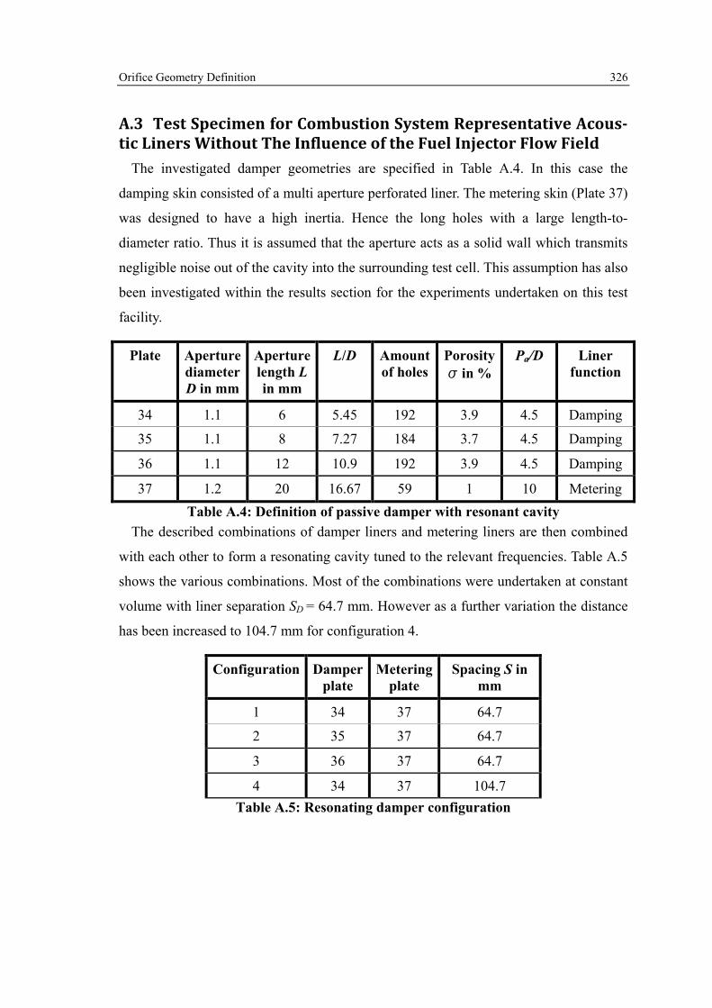
Orifice Geometry Definition 326
A.3 Test Specimen for Combustion System Representative Acous-tic Liners Without The Influence of the Fuel Injector Flow Field
The investigated damper geometries are specified in Table A.4. In this case the
damping skin consisted of a multi aperture perforated liner. The metering skin (Plate 37)
was designed to have a high inertia. Hence the long holes with a large length-to-
diameter ratio. Thus it is assumed that the aperture acts as a solid wall which transmits
negligible noise out of the cavity into the surrounding test cell. This assumption has also
been investigated within the results section for the experiments undertaken on this test
facility.
Plate Aperture diameter D in mm
Aperture length L in mm
L/D Amount of holes
Porosity s in %
Pa/D Liner function
34 1.1 6 5.45 192 3.9 4.5 Damping
35 1.1 8 7.27 184 3.7 4.5 Damping
36 1.1 12 10.9 192 3.9 4.5 Damping
37 1.2 20 16.67 59 1 10 Metering Table A.4: Definition of passive damper with resonant cavity
The described combinations of damper liners and metering liners are then combined
with each other to form a resonating cavity tuned to the relevant frequencies. Table A.5
shows the various combinations. Most of the combinations were undertaken at constant
volume with liner separation SD = 64.7 mm. However as a further variation the distance
has been increased to 104.7 mm for configuration 4.
Configuration Damper plate
Metering plate
Spacing S in mm
1 34 37 64.7
2 35 37 64.7
3 36 37 64.7
4 34 37 104.7 Table A.5: Resonating damper configuration

Orifice Geometry Definition 327
A.4 Damper Test Geometry for Acoustic Dampers Exposed to Fuel Injector Flow Field
The damper geometries exposed to a representative fuel injector flow field are
discussed in this section; the fuel injector geometry will not be presented as its
geometry is confidential. Table A.6 specifies the geometric definition for the
investigated passive damping system. All the orifices within the damping skin and
metering skin were cylindrical and drilled normal to the liner surface. The damping skin
was optimised so that a high porosity for a minimised pressure drop could be achieved.
However a minimum pressure drop is required so there is no steady inflow of hot gases
from the combustor into the damper cavity. Moreover, the amount of air for such a
system is specified by the wall cooling budget of the gas turbine combustor. Hence the
maximum porosity available cannot exceed the wall cooling budget of the system.
The damping skin and the metering skin were separated to form a rectangular cavity.
This cavity was not tuned to resonate at the frequencies investigated. A sensitivity of the
distance between the damping skin and metering skin was conducted. Therefore the
separation was varied throughout the experiments from 4611250 .. ≤≤ HS , where H is
the height of the duct as shown in Figure 3.9.
Liner Aperture diameter D in mm
Aperture length L in mm
L/D Amount of holes
Porosity
s in %
Pa/D Shape
Damping liner
0.7 2 2.86 1490 3.56 4.3 Cylindrical
Metering liner
1 2 2 252 1.23 7.2 Cylindrical
Table A.6: Definition of passive damper for non-resonant cavity experiments

Effective Flow Area Experiments 328
B. Effective Flow Area Experiments A variation of orifice plates are investigated in terms of their acoustic absorption
characteristic. As already discussed in the previous chapters the acoustic absorption of
an aperture is dependent on the mean flow Strouhal number across the orifice equation
(1.16). This Strouhal number definition uses the velocity in the plane of the aperture.
Thus the discharge coefficient of the orifice geometry has to be known for the
calculation of the mean velocity in the plane of the aperture based on the measured
mean velocity at the end of the vena contracta:
dDD UCU = . ( A.1)
The discharge coefficient can be calculated from a known mass flow and pressure
difference across the orifice as defined in equation (2.5). Thus a test rig has been used to
measure the discharge coefficient for steady state flow conditions. The test rig consisted
of a plenum chamber of 3763 mm3. All the investigated orifice plates (Table A.1 - A.3)
were connected to this volume. A Cole Parmer 0-250 SLPM (standard liters per minute)
air mass flow meter was used to accurately measure the air flow rate into the plenum
chamber. Moreover the static pressure inside the plenum was measured using a tapping
connected to Furnace FC0510 Micro-Manometer. And finally the air temperature was
measured using a K-Type thermo-couple within the plenum chamber connected to a
TME Model 6000 Thermocouple thermometer. The accuracy of the mass flow meter
was %.80± of reading +0.2% of full scale (Cole-Parmer (2009)). Moreover the
accuracy of the Micro-Manometer was ± 0.1% and the temperature measurement is of
the order of ± 0.6 C as indicated on the TME data sheet. This can therefore lead to an
accuracy of the discharge coefficient measurement of ± 1%.
The steady state discharge coefficients have been measured for mean pressure drops
across the orifice of dp/p = 0.1%-1.0%. This results in Reynolds numbers larger than
7000 which is sufficient for the measured discharge coefficients to remain constant with
changing pressure drop as indicated in Lichtarowicz et. al. (1965).

Validation of the Methodology to Identify the Acoustically Related Flow Field 329
C. Validation of the Methodology to Identify the Acoustically Related Flow Field
In this section the validation of the developed methodology to identify the
acoustically related flow field will be described as in Rupp et. al. (2010b). Initially the
acoustically related flow field relevant to the non-linear acoustic absorption will be
validated and subsequently the linear acoustic absorption regime. The validation will be
based on the acoustic absorption measurements discussed in chapter 5 and 6.
C.1 Kinetic Energy Balance - Non-Linear Absorption Regime To validate the methodology, and its ability to identify the flow structures associated
with acoustic absorption, the energy content of the flow field can be considered. Energy
to drive the total velocity field can originate either from (i) the centrifugal fan used to
draw air through the test section or (ii) or the loudspeakers generating a pressure wave
which controls the unsteady pressure drop across the aperture. The energy derived from
the centrifugal fan can be determined by the mean pressure drop across the orifice and
the volume flow rate i.e.
Vp ∆Π = . ( C.1)
The acoustic energy loss was calculated from the difference in the flux of acoustic
energy going towards (in), and away from (out) the orifice for each side of the orifice.
The acoustic energy flux was calculated as
( )22 pM1
c2A ±± ±=ρ
Π ( C.2)
and hence the loss of acoustic energy is defined as
±± −= outin ΠΠΠ . ( C.3)
For non-linear absorption only a small amount of air was drawn through the test section.
Hence for the total velocity field typically 5% of the energy originated from the
centrifugal fan with 95% being absorbed from the acoustic field. The kinetic energy in

Validation of the Methodology to Identify the Acoustically Related Flow Field 330
the flow field was calculated using a similar method as described in Tam and Kurbatskii
(2000). The flow field was assumed to be axis-symmetric as indicated in the schematic
in Figure C.1. The kinetic energy is defined as:
221
umEkin
= . ( C.4)
In this case the mass is defined as:
Vm ρ= . ( C.5)
Thus the kinetic energy within the flow field has to be integrated over the total
cylindrical volume:
( ) ( )( )∫ ∫ +=L R
kin dydrrtrvtruE0 0
22 ,,ρπ . ( C.6)
The radius is then replaced by the coordinate x and the integrals is replaced by a
numerical summation:
( ) .max max∑ ∑ +=
Y X
kin dydxxvuE0 0
22ρπ . ( C.7)
This, of course, is calculated from the acoustically related reconstructed flow field for
every recorded time step.
A further point that needs to be considered is, for the non-linear absorption case,
whether the mean flow should be included in the reconstructed flow field from which
the kinetic energy is calculated. Intuitively one might suspect that the mean flow field
should not be included. However, as already indicated the acoustic field is responsible
for generating vortex ring type structures which induces a mean velocity field. This
mean flow field is responsible for the convection of each ring structure away from the
orifice. This is further suggested by the change in the mean velocity field that was
observed for the case with and without excitation (Figure C.2). Hence some of the
energy absorbed from the acoustic field must be present in the mean flow field. Thus the
reconstructed flow field consists of the mean flow field (with excitation) together with
all the ‘acoustic related’ modes. The kinetic energy loss associated with the centrifugal

Validation of the Methodology to Identify the Acoustically Related Flow Field 331
fan (equation ( C.1)) must then be subtracted from the kinetic energy of the
reconstructed ‘acoustically related’ flow field.
An example of the total kinetic energy calculated from the upstream and downstream
reconstructed flow fields can be seen in Figure C.3 at various time steps during the
acoustic cycle. Note that the frequency at which the PIV measurements were obtained
(1100 Hz) was not a multiple of the acoustic excitation frequency (125 Hz). This was
done to ensure data was obtained at all phases of the excitation cycle during the period
of data capture and accounts for the slight variations in the kinetic energy maxima
observed between acoustic cycles. It can be seen that the energy shows a maximum in
the upstream and downstream field exactly once per cycle. In reality the fluctuating
pressure drop across the orifice caused by the acoustic waves generates a pulsatile flow
within the orifice and, as flow is discharged from the orifice, a ring vortex structure is
generated. As this structure grows so the kinetic energy associated with this structure
increases. Eventually the structure is swept away from the orifice and the kinetic energy
within the field of view decreases. This phenomenon happens once per cycle either side
of the orifice and is reflected in the observed variations in kinetic energy (Figure C.3).
Note that the small mean flow through the orifice is responsible for the greater energy
observed within the downstream vortex structures. The maxima of the kinetic energy
have been averaged and divided by the time period of one acoustic cycle:
TEkin=Π . ( C.8)
The maximum energy loss as well as the averaged energy loss was then compared to
the acoustic loss as shown in Figure C.4. The maximum acoustic energy loss was
calculated using the maximum measured energy in the upstream and downstream flow
field (e.g. 6.5x10⁻⁴ J downstream and 4.1x10⁻⁴ J upstream in Figure C.3). The mean
energy loss was calculated by ensemble averaging the energy maxima in the upstream
and downstream flow field. It can be seen that the energy calculated using the
reconstructed flow fields agree with the energy that is being absorbed from the acoustic
field. The discrepancies are caused if the maximum kinetic energy within the vortex
ring structure is not captured within the measured flow fields. Hence the maximum
kinetic energy shows the better agreement with the method. Moreover some of the

Validation of the Methodology to Identify the Acoustically Related Flow Field 332
kinetic energy might have already been lost due to viscous dissipation. This is already a
very good indication that the reconstructed acoustically related flow field is
representative of the flow field associated with the acoustic absorption. More evidence
for this conclusion can be found in the following section where the energy flux balance
is used within the non-linear and linear regime.
C.2 Energy Flux Balance – Non-Linear and Linear absorption Re-gime
The fluid dynamics of the linear absorption process makes it difficult to apply the
same method used previously for validating the methodology. This is due to the
continuous shedding of coherent structures which gives rise to issues associated with
identifying which structures are related to a given acoustic cycle, are all the structures
captured in the field of view etc. In addition, the scale of these structures means that the
transfer of energy into the random turbulent flow field will occur relatively quickly i.e.
so some of the absorbed energy will be present in the random turbulent POD modes
rather than the ‘acoustic related’ modes. Hence an alternative method has to be adopted,
which can be used within the linear and non-linear absorption regime.
The kinetic energy flux of the flow, normal to the x-z-plane (Figure C.5), was
calculated for various downstream locations and instances in time. This was done using
the flow field reconstructed from the ‘acoustic related’ modes. The acoustic energy flux
is defined as
221 vmE = . ( C.9)
Moreover the mass flow through the aperture can be defined using the v-velocity
component and an integration across the circular aperture area. Hence the kinetic energy
flux at a given radius r and time t can be defined as:
( ) ( ) dAtrvtrvEd 221
,, ρ= . ( C.10)
Using a circular area just downstream the orifice and integrating over the radial
coordinate results in (e.g. Pope (2000))

Validation of the Methodology to Identify the Acoustically Related Flow Field 333
( ) ( ) ( )∫ +=R
drrtrvtrutrvE0
22 ),,(,ρπ . ( C.11)
Thus the kinetic energy flux of the flow field through the aperture was expressed using
the x-coordinate in radial direction:
( ) ( ) ( )∑ ∆+=max
),,(,X
xxtxvtxutxvE0
22ρπ . ( C.12)
C.2.1 Non-Linear Absorption Regime The kinetic energy flux, as defined in equation ( C.12), was applied immediately
upstream and downstream of the orifice as indicated in Figure C.6. The actual
coordinate in the upstream and downstream flow field for the integration of the kinetic
energy flux is defined in Table C.1.
y/D
Upstream Downstream
131 dB 0.03 -0.07
137 dB 0.03 -0.07
142 dB 0.06 -0.07 Table C.1: Coordinates for energy flux calculation for flow field associated with
the non-linear acoustic absorption regime The result of this integration for some instances in time is shown in Figure C.7. The
change in sign is due to the change in flow direction. The PIV measurement was
triggered and thus synchronised with the function generator input to the loudspeakers.
Therefore the phase relationship between the velocities in the upstream and downstream
flow fields remained constant. Hence the maximum energy flux in the upstream and
downstream flow field is 180° out of phase. During the low pressure part of the acoustic
cycle the fluid is accelerated to the downstream side of the orifice and the maximum
kinetic energy flux occurs on the downstream side, i.e. time step ~3 in Figure C.7.
During the maximum pressure part of the acoustic cycle, the fluid is accelerated
upstream and the maximum kinetic energy flux occurs in the upstream side of the
aperture, i.e. time step 8 in Figure C.7. Moreover increases caused by the acceleration of
the fluid into the aperture can also be seen, e.g. time step 3 in the upstream field and 8

Validation of the Methodology to Identify the Acoustically Related Flow Field 334
in the downstream field. Hence the total kinetic energy flux averaged over the acoustic
cycle can be calculated by investigating the kinetic energy flux of equal sign on each
side of the aperture as indicated in Figure C.8. In this case the absolute of the kinetic
energy flux in the downstream field was used. The averaged kinetic energy flux per
acoustic cycle was then calculated by integrating both curves upstream and downstream
of the aperture relative to the total sampling time of the velocity measurements:
( ) ( )∫ ′+′=+=T
0du21 dtEE
T1
AAT1
'E . ( C.13)
As already discussed both sides of the apertures are important during non-linear
absorption as reverse flow is occuring. Hence the acoustic loss per cycle is split between
the upstream and downstream flow fields. Furthermore as already discussed, the kinetic
energy introduced by the centrifugal fan has to be deducted. In this case the kinetic
energy flux of the mean flow field without excitation was calculated as shown in Figure
C.9. Therefore the mean kinetic energy flux at y/D = -0.07 has been deducted from the
unsteady kinetic energy flux of the forced case:
unforcedEE −=Π ' . ( C.14)
The comparison between the calculated kinetic energy flux and the measured acoustic
loss is shown in Figure C.10. The agreement between the acoustic energy loss and the
kinetic energy flux within the acoustically related flow field is very good. Hence it can
be concluded that the developed methodology is capturing the relevant fluid dynamic
characteristics important to the non-linear acoustic absorption very well.
C.2.2 Linear Absorption Regime Within the linear absorption regime, both the kinetic energy flux for the mean flow
and the instantaneous flow are important and need to be calculated. The kinetic energy
flux of the mean flow field E is presented in Figure C.11 for an unsteady jet flow of
0.8% and 0.3% dp/p within the linear absorption regime where, as expected, the
maximum energy flux occurs close to the orifice. The decreasing nature of the energy
flux further downstream reflects the transfer of energy into random turbulence.

Validation of the Methodology to Identify the Acoustically Related Flow Field 335
The instantaneous kinetic energy flux 'E of the filtered flow, including the mean flow
field, is shown in Figure C.12 at a location close to the orifice exit plane (i.e. so that
only a small amount of energy has been dissipated into random turbulence). The data is
presented for several acoustic cycles. The variation in kinetic energy reflects the
pulsatile nature of the flow through the orifice due to the effect of the oscillating
pressure drop on the jet flow. The peaks and troughs represent the points where the
pulsatile flow reaches its maximum and minimum velocities. Note also that the case of
0.8% dp/p shows a larger modulation, relative to 0.3% dp/p, due to the larger excitation
amplitude (137dB and 128dB respectively). For the current experimental configurations
the acoustic energy transmitted through the orifice is several orders of magnitude less
than the acoustic energy absorbed by the orifice. In other words all the energy
associated with this pulsatile flow is being absorbed from the acoustic field. This
pulsatile flow then generates the turbulent structures observed in the reconstructed flow
field and which eventually decay into random turbulence.
This can be confirmed by comparing the acoustic energy being absorbed with the
kinetic energy flux of the pulsatile flow. The instantaneous energy flux is therefore
integrated over a complete cycle from which the mean energy flux has to be subtracted
i.e.
EE −=Π ' . ( C.15)
As already mentioned the mean energy flux is generated by the mean pressure drop due
to the work input by the centrifugal fan. Figure C.13 shows, in contrast with the non-
linear absorption the mean flow field with and without excitation is nearly identical.
Hence it can be assumed that all the kinetic energy contained in the mean flow field is
related to the work of the centrifugal fan. Thus the mean kinetic energy flux has to be
deducted from the acoustically related kinetic energy flux (equation ( C.15)).
The resulting energy flux is then compared to the acoustic energy loss. The loss of
acoustic energy and the acoustic absorption coefficient has been measured
simultaneously while measuring the velocity field using PIV. PIV experiments for the
9.1 mm diameter orifice plate with length-to-diameter ratios of 0.5, 1, 2, 3 and 5 have
been conducted with excitation amplitudes as indicated in Figure C.14 and 62.5 Hz

Validation of the Methodology to Identify the Acoustically Related Flow Field 336
excitation frequency. All of this data has then been compared to the measured acoustic
energy loss in Figure C.15. It can be seen that the agreement between the acoustic
energy loss and the measured acoustic energy flux is excellent for all the considered test
cases. Moreover the filtering of the acoustically related modes is necessary to be able to
identify the relevant flow properties carrying the relevant kinetic energy flux. As it can
be seen the kinetic energy calculated by the total velocity field, i.e. the raw velocity
field, would show far more energy than the measured acoustic energy loss. The PIV
methodology of the acoustically related flow field was within 20% of the acoustic loss
measurement, which is most likely the resolution of this challenging PIV application.

Validation of the Methodology to Identify the Acoustically Related Flow Field 337
Figures
Figure C.1: Schematic of control volume of kinetic energy calculation in the non-
linear absorption regime
Figure C.2: Example of forced and unforced mean flow field, non-linear acoustic
absorption, L/D = 0.47, f = 125 Hz, plate number 1.
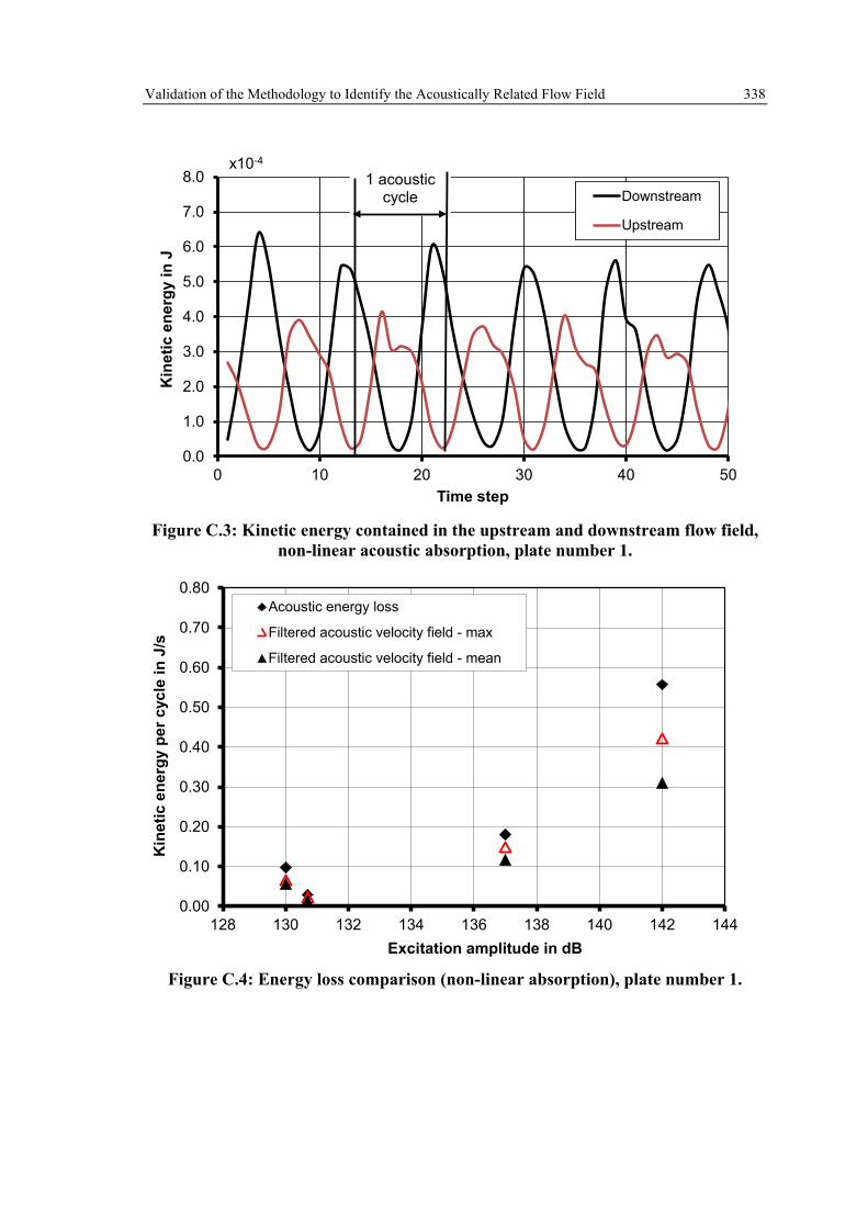
Validation of the Methodology to Identify the Acoustically Related Flow Field 338
0.0
1.0
2.0
3.0
4.0
5.0
6.0
7.0
8.0
0 10 20 30 40 50
Kin
etic
ene
rgy
in J
Time step
Downstream
Upstream
x10-4
1 acousticcycle
Figure C.3: Kinetic energy contained in the upstream and downstream flow field,
non-linear acoustic absorption, plate number 1.
0.00
0.10
0.20
0.30
0.40
0.50
0.60
0.70
0.80
128 130 132 134 136 138 140 142 144
Kin
etic
ene
rgy
per c
ycle
in J
/s
Excitation amplitude in dB
Acoustic energy loss
Filtered acoustic velocity field - max
Filtered acoustic velocity field - mean
Figure C.4: Energy loss comparison (non-linear absorption), plate number 1.

Validation of the Methodology to Identify the Acoustically Related Flow Field 339
r, x, uR
y, v
v
r, x, uR
y, v
Circular planenormal to the
x,y - planeNon-linear absorption Linear absorption
Figure C.5: Schematic of control surface for energy flux calculation
Figure C.6: Schematic of integral location upstream and downstream of the aper-
ture, non-linear absorption regime, L/D = 0.47, 137 dB, 125 Hz, plate number 1

Validation of the Methodology to Identify the Acoustically Related Flow Field 340
-0.8
-0.6
-0.4
-0.2
0
0.2
0.4
0.6
0.8
0 5 10 15 20
Inst
anta
neou
s ki
netic
ene
rgy
flux
in J
/s
Time step
Downstream
Upstream1 acoustic cycle
Figure C.7: Instantaneous kinetic energy flux of the aperture, non-linear absorp-
tion regime, L/D = 0.47, 137 dB, 125 Hz, plate number 1.
-0.8
-0.6
-0.4
-0.2
0
0.2
0.4
0.6
0.8
0 5 10 15 20
Kin
etic
ene
rgy
flux
in J
/s
Time step
Downstream
Upstream
A1 A2
Figure C.8: Absolute instantaneous kinetic energy flux upstream and downstream
of the aperture, non-linear absorption regime, L/D = 0.47, 137 dB, 125 Hz, plate number 1.

Validation of the Methodology to Identify the Acoustically Related Flow Field 341
0.0
0.5
1.0
1.5
2.0
2.5
3.0
-2.5-2-1.5-1-0.50
Kin
etic
ene
rgy
flux
in m
J/s
y/D Figure C.9: Schematic of mean energy flux, no excitation, L/D = 0.47, dp = 8 Pa,
plate number 1
0.00
0.10
0.20
0.30
0.40
0.50
0.60
0.70
0.80
128 130 132 134 136 138 140 142 144
Aver
aged
kin
etic
ene
rgy
flux
in J
/s
Excitation amplitude in dB
Acoustic energy loss
Filtered acoustic velocity field
Figure C.10: Averaged kinetic energy flux per acoustic cycle compared to acoustic
energy loss, non-linear absorption regime, L/D = 0.47, plate number 1.
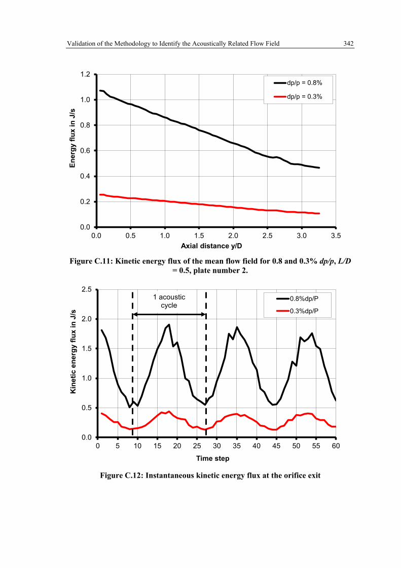
Validation of the Methodology to Identify the Acoustically Related Flow Field 342
0.0
0.2
0.4
0.6
0.8
1.0
1.2
0.0 0.5 1.0 1.5 2.0 2.5 3.0 3.5
Ener
gy fl
ux in
J/s
Axial distance y/D
dp/p = 0.8%
dp/p = 0.3%
Figure C.11: Kinetic energy flux of the mean flow field for 0.8 and 0.3% dp/p, L/D
= 0.5, plate number 2.
0.0
0.5
1.0
1.5
2.0
2.5
0 5 10 15 20 25 30 35 40 45 50 55 60
Kin
etic
ene
rgy
flux
in J
/s
Time step
0.8%dp/P
0.3%dp/P
1 acousticcycle
Figure C.12: Instantaneous kinetic energy flux at the orifice exit

Validation of the Methodology to Identify the Acoustically Related Flow Field 343
Figure C.13: Example of forced and unforced mean flow field, linear acoustic ab-
sorption, L/D = 1, f = 62.5 Hz, 0.8% dp/p, plate number 3. L/D = 0.5
0.0
0.1
0.2
0.3
0.4
0.5
0.6
0.7
120 130 140 150
Abso
rptio
n co
effic
ient
Excitation amplitude in dB
dp/p = 0.8%dp/p = 0.5%dp/p = 0.3%dp/p = 0.1%PIV data points
L/D = 3
0.0
0.1
0.2
0.3
0.4
120 130 140 150
Abso
rptio
n co
effic
ient
Excitation amplitude in dB
dp/p = 0.5%dp/p = 0.3%dp/p = 0.1%PIV data points
Figure C.14: PIV data points relative to measured absorption coefficients
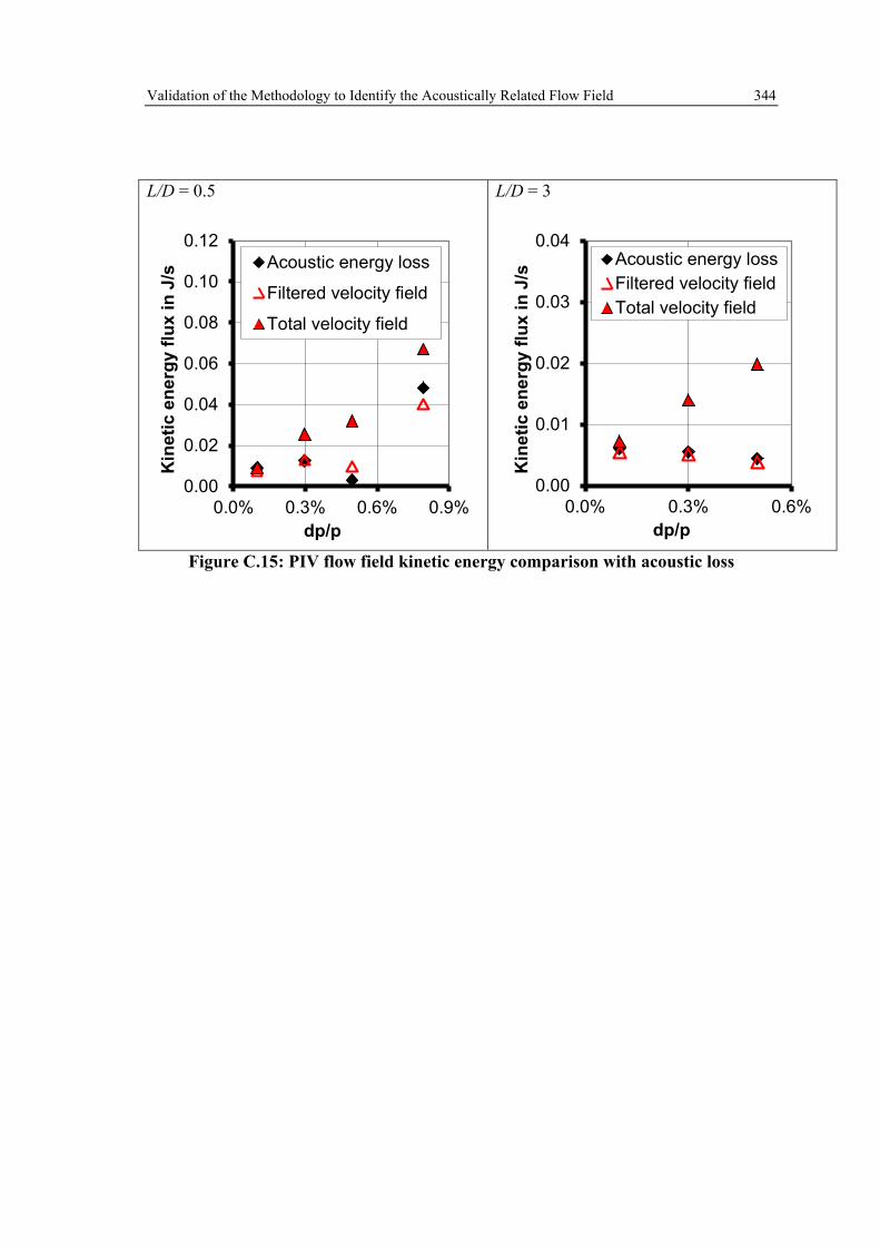
Validation of the Methodology to Identify the Acoustically Related Flow Field 344
L/D = 0.5
0.00
0.02
0.04
0.06
0.08
0.10
0.12
0.0% 0.3% 0.6% 0.9%
Kin
etic
ene
rgy
flux
in J
/s
dp/p
Acoustic energy loss
Filtered velocity field
Total velocity field
L/D = 3
0.00
0.01
0.02
0.03
0.04
0.0% 0.3% 0.6%K
inet
ic e
nerg
y flu
x in
J/s
dp/p
Acoustic energy lossFiltered velocity fieldTotal velocity field
Figure C.15: PIV flow field kinetic energy comparison with acoustic loss

Phase Averaging of Acoustically Related Velocity Field 345
D. Phase Averaging of Acoustically Related Velocity Field
To get a more meaningful characterisation of the velocity field the filtered
acoustically related flow field has been phase averaged. However, as the excitation
frequency is 125 Hz and the PIV sampling frequency is 1100 Hz this is not
straightforward. Hence the temporal coefficient of each acoustically related POD mode
has been interpolated using the Fast Fourier interpolation technique in MATLAB.
Therefore the sampling frequency has been increased by factor 5 leading to 44 phases
for one acoustic cycle at 125 Hz forcing frequency. Moreover 70 instances for each
phase along the acoustic cycle have then been averaged. An example of the statistical
accuracy of this data can be found in Figure D.1 for the best case and Figure D.2 for the
worst case. The data shows a deviation of the true mean (at 0%) to the actual mean
velocity calculated by the amount of samples. This deviation, and the standard error, has
been normalised relative to the mean velocity over half an acoustic cycle:
( )∫=2
0
2T
bulk dttUT
U . ( D.1)
The standard errors have been calculated as in Montgomery and Runger (1994):
Nzu
1σε =,
( D.2)
where z represents the confidence band, which is defined as 2.576 for a 99% band and
1.96 for a 95% band. Moreover the parameter σ represents the standard deviation of the
sample and N denotes the amount of samples. In the worst case scenario of t/T = 0.45
where the velocity at x/D = 0 and y/D = -0.07 is close to zero the error estimated for the
statistical accuracy of the phase average velocity is no worse than 4% for a 95%
confidence band. Hence the estimate for the phase averaged acoustically related flow
field was seen as sufficient in terms of its statistical accuracy.
Furthermore the acoustically related flow field during linear acoustic absorption was
also phase averaged. The only difference to the non-linear acoustic absorption flow field

Phase Averaging of Acoustically Related Velocity Field 346
is that in the linear regime the forcing frequency was set to 62.5 Hz. Hence the data was
interpolated using the MATLAB Fourier spectrum interpolation based on 7680 samples
and an interpolated sampling frequency of 2750 Hz. This has also led to 70 samples per
phase average. Figure D.3 shows the statistical accuracy of the phase average at t/T =
0.5 which is the velocity minimum for the considered orifice geometry. In this case the
deviation from the true mean has been normalised relative to the mean v-velocity
component at the exit of the aperture for the test case. As it can be seen the statistical
accuracy is within 3% for a 99% confidence band.
Figure D.1: Example of best case statistical analysis of phase average data, 137 dB
excitation amplitude, t/T = 0.3, L/D = 0.47, plate number 1.

Phase Averaging of Acoustically Related Velocity Field 347
Figure D.2: Example of worst case statistical analysis of phase average data, 137
dB excitation amplitude, t/T = 0.45, L/D = 0.47, plate number 1.
Figure D.3: Example of worst case statistical analysis of phase average data, dp/p =
0.8%, t/T = 0.5, L/D = 0.5, plate number 3.

Circumferential wave considerations 348
E. Circumferential wave considerations As already discussed the damper test facility, described in chapter 3.3.2, used for the
non-resonant acoustic damper investigation (section 8.2) was simulating one sector of a
full annular combustor. Plane axial acoustic waves were used to measure the acoustic
performance of the damper system exposed to a realistic flow field generated by a fuel
injector. This resulted in an axial acoustic standing wave with its anti-node being at the
fuel injector exit extending over the face of the damping skin. Figure E.1 shows a
schematic of an axial cut through a full annular combustor rotated around the centreline
(CL). Moreover a front view along the line (A-A’) of a schematic full annular combustor
is shown on the right hand side of Figure E.1. In this case a passive damping system is
applied to the outer combustor wall. In practice full annular combustion systems are
prone to combustion instabilities coupling with circumferential pressure waves
travelling in the azimuthal direction. For the experiments and modelling conducted in
the previous section it was assumed that the azimuthal change in pressure amplitude
was small. Hence the pressure amplitude would remain constant along the
circumferential coordinate as long as the damper length in circumferential direction is
much smaller than the wave length, i.e. long wave length assumption in circumferential
direction. However the designer of an acoustic damping system might want to extend
the damper volume over more than one sector or ultimately would like to assess if the
total annulus between the metering skin and damping skin can be used for the passive
damper. If no separating walls between the damper cavity is used, i.e. full annular cavity
between metering and damping skin, the azimuthal modelling developed by Eldredge
(2004) can be applied. However very little is known using separated cavities within the
annulus between the damping and metering skin. Hence a design tool is proposed for
the acoustic absorption assessment of the circumferential length of the damper cavity.
E.1 Definition of Circumferential Wave Model A model was developed to simulate a travelling wave along the surface of the damper
with the emphasis of the assessment of the cavity acoustics between damping and

Circumferential wave considerations 349
metering skin. This model is described in this section. Therefore the circumferential
combustor as shown in Figure E.1 was modelled as an axial duct where the axial length
is representing the circumferential length of the damper segments as indicated in Figure
E.2. Hence the circumferential coordinate in the full annular system was replaced by the
axial coordinate x. Moreover the circumferential length of the damping segments is
represented by the parameter LD. In this case waves perpendicular to the axial
coordinate x, i.e. axial waves and radial waves within the full annular combustion
system are neglected, as they are below the cut-off frequency for the considered
frequency range (below 1000 Hz at full engine operating conditions). Another
simplification has been incorporated by assuming the metring skin of the damping
system is fed by a plenum, i.e. the pressure amplitude upstream of the metering skin is
set to zero. In reality the metering panel will be fed by a thin annulus between the
metering skin and the engine casing. However, the model is used as a preliminary
design tool for the damper geometry and so this detail is initially neglected.
Nevertheless this should be incorporated in more detailed network representations for
the linear stability analysis of a fully representative combustion system.
The input to the developed model is an axial travelling wave with a given amplitude
0p which is introduced to simulate a travelling wave within the combustion system.
Therefore the travelling wave is defined as
( ) ( )ikxpxp exc −= expˆˆ0 . ( E.1)
In the previously developed model the long wave length assumption was used
assuming there is no change in pressure amplitude along the coordinate x. However in
this case this needs to be incorporated to assess the acoustic mode shapes within the
cavity between damping and metering skin. According to Eldredge and Dowling (2003)
the change in stagnation enthalpy relative to the axial coordinate can be described in
non-dimensional form as
CC uikL
dxBd ˆˆ
−= . ( E.2)
Moreover the change in acoustic velocity amplitude within the cavity with respect to
the axial coordinate was defined as

Circumferential wave considerations 350
22
11 v
ALC
vA
LCBikL
dxud
C
D
C
DC
C ˆˆˆˆ+−−= .
( E.3)
For the purpose of this work mean velocity is only present across the metering and
damping skin. Within the duct representing the combustion chamber there will be no
mean flow in the axial direction, i.e. no mean flow component in circumferential
direction for the full annular combustion system. Moreover the damping skin and
metering skin forms a rectangular cavity of length LD, width WD and height S. Hence
reintroducing the dimensions into equations ( E.2) and ( E.3) and changing the geometric
parameters for the circumference (C1 and C2) and cross-sectional area (AC) of the
tubular damper cavity into a rectangular cavity leads to the change in cavity pressure
amplitude in axial direction
( ) ( )xuidx
xpdCˆ
ˆρR−=1
( E.4)
and change in axial acoustic velocity amplitude in axial direction
( ) ( ) ( ) ( )xvS
xvS
xpp
idx
ud xC211
1
111 ˆˆˆˆ
+−−=γ
R ( E.5)
with respect to time and space. In this case the velocity amplitude over the damping
skin can be defined as in Eldredge and Dowling (2003) or Rupp et. al. (2012):
( ) ( ) ( )
−=
0
0
1
12
11 p
pp
pL
cωjη
vγγ
xxx .
( E.6)
Moreover the metering skin velocity amplitude is defined in the same way
( )
−=
1
12
22 p
pL
cωjη
vγ
x.
( E.7)
The parameter η represents the compliance of the perforated liner. According to
Eldredge and Dowling (2003) the compliance is defined as
DDD LL
KLR
σσπ
η+=
11 2.
( E.8)

Circumferential wave considerations 351
In this case the compliance is representing the modified Howe model as discussed in
section 2.5.2 or 5.8 with the Rayleigh Conductivity defined as in Howe (1979b)
( ) ( )StiStpvRiKD δRρπ
+Γ=−
=ˆˆ
2.
( E.9)
As discussed in section 5.9 the model utilising the linear solution of the unsteady
momentum balance is a more intuitive and accurate representation of the linear acoustic
absorption characteristics for acoustic dampers within gas turbine combustors. Hence
the Conductivity terms used by Eldredge and Dowling (2003) have been modified so
that they are calculated form the liner impedance of the damping and metering skin
( ) ( )Z
RiStiSt 12
Rρπδ −=+Γ .
( E.10)
The liner impedance Z was defined as in chapter 5.9:
111211
011
1 LiUCv
ppZ visD
DDρRρζρ ++=
−= ,ˆ
ˆˆ,
( E.11)
222222
12
1 LiUCv
pZ visD
DDρRρζρ ++=
−= ,ˆ
ˆ.
( E.12)
Thus the compliance used in travelling wave model in this section is then based on
the Conductivities of the damping and metering skin using the impedance of the liners
derived from the unsteady momentum balance as defined in equations ( E.11) and
( E.12):
( )R
iLDπ
δση
+Γ=
2.
( E.13)
The compliance is then used in equations ( E.6) and ( E.7) to define the unsteady
velocity amplitudes across the damping skin and metering skin. Thereafter the velocities
are substituted into equation ( E.5)
( ) ( ) ( )0
02
1
1
12
22
1 111p
xpLc
iSpxp
Lc
iSLc
iSi
dxxud
DDD
CγR
ηγR
ηR
ηR
ˆˆˆ+
−−−= .
( E.14)

Circumferential wave considerations 352
This equation can then be differentiated with respect to the axial coordinate and
equation ( E.4) can be substituted for the differential of pressure amplitude in the cavity
with respect to the axial coordinate. Hence an inhomogeneous ordinary differential
equation of second order can be derived
( ) ( ) ( )ikxxudx
xudC
C −=− expˆˆ
βα2
2.
( E.15)
The time and space independent constant α is therefore defined as
( )ρRγR
ηγR
ηγ
Rα ipL
ciSpL
ciSp
iDD
−−−=
1
22
1
21
1
11111 . ( E.16)
and the constant β is defined as
excD
ppL
ciS
ik ˆ0
21 11
γRη
β −= . ( E.17)
This differential equation can be solved analytically as a superposition of the general
solution for a homogenous differential equation and the particular solution of the
inhomogeneous equation. The particular solution was derived based on the right hand
solution of the differential equation ( E.15). Hence the acoustic velocity amplitude in the
damper cavity with respect to time and axial coordinate x can be defined as
( ) ( ) ( )( )
( )ikxik
xConstxConsttxuC −−−
+−+= expexpexp,ˆα
βαα 221 . ( E.18)
The time dependent constant Const1 and Const2 can be derived using the boundary
conditions for the systems. As the volume is enclosed by rigid walls the boundary
conditions can be defined so that the acoustic velocity amplitude vanishes at the walls
of the cavity volume, i.e.
( ) ( ) 00 ==== DCC Lxuxu ˆˆ . ( E.19)
Thus the time dependent constants can be defined as
( ) 221 Constik
Const −−−
−=α
β ( E.20)

Circumferential wave considerations 353
and
( )( ) ( )
( ) ( )DD
DDLLLikL
ikConst
ααα
αβ
expexpexpexp
−−
+−−
−−= 22 .
( E.21)
The cavity pressure amplitude mode shape can then be calculated by differentiating
the cavity velocity amplitude (equation ( E.18)) with respect to the axial coordinate x
and substituting it into equation ( E.14). Thereafter the velocity amplitudes can be
calculated using the incident pressure amplitude and the cavity pressure amplitudes in
equations ( E.6) and ( E.7).
Finally the acoustic energy loss is derived as proposed by Eldredge and Dowling
(2003) in non-dimensionalised form for tubular damping and metering skin with
circumference C1 and C2
( ) ( ) ( ) ( )
+
=′=Π ∫∫∫
1
0
22
21
21
0
21
1
1
01
112
dxxvCC
dxxvkL
dxxvxB DL ˆImˆ'
ηη.
( E.22)
This equation was dimensionalised and the velocity amplitudes have been numerically
integrated along the axial coordinate of the damper surface:
( ) ( )
+
=Π ∫∫
DLDL
DDL dxxvdxxvWL0
22
20
21
1
1121 ˆImˆIm
ηηRρ .
( E.23)
Finally the calculated energy loss along the acoustic damper was normalised with the
incident pressure amplitude
2exc
LP
p
Π=Π .
( E.24)
E.2 Circumferential Modelling Results for the Example of a Reso-nating Liner
The developed circumferential acoustic absorption model was used to assess the
acoustic characteristics of resonant liners exposed to travelling waves. One aspect of
this investigation is to assess at which point the resonance behaviour in the cavity
between metering and damping skin is breaking down and thus reduces the generated

Circumferential wave considerations 354
acoustic energy loss. During the design process it is cost effective to validate and
optimise acoustic damper designs exposed to axial acoustic waves in impedance test
facilities. Nevertheless if the damper is applied to full annular gas turbine combustors
suffering from circumferential travelling waves it is important to analyse if the damper
cavity is able to resonate and the long wave length assumption within the damper cavity
is still valid. Hence the circumferential model has been applied to the resonant damper
configuration 1 (details of the test specimen can be found in section A.3). In this case
the resonant liner is mounted as shown in Figure E.1 and Figure E.2 (unlike the
experimental results shown in section 8.3.1 where the damper was mounted
perpendicular to the axial wave). The initial analytical model describing the cavity
pressure amplitude with a single point (i.e. incident pressure amplitude if the damper is
mounted perpendicular to an incident axial wave), assuming the long wave length
assumption as used in chapter 8. Hence for an initial validation of the circumferential
modelling behaviour the resonant liner configuration using the “single point model” was
compared to the circumferential travelling wave model. The length of the damper LD
was set to the circumferential width of one sector of a reference full annular test facility.
Figure E.3 shows a comparison between the calculated acoustic energy loss by the
single point model and the travelling wave model for the resonant damper configuration
1. In general the two models are nearly identical for the chosen sector length. Both
models show the same amount of acoustic absorption and predict the resonance
frequency to 500 Hz. In general the effects of a travelling wave upon the absorption of
the investigated single sector damper configuration seem to be negligible within the
investigated frequency band. Discrepancies between the two models occur for
frequencies larger than 600 Hz and this deviation seems to increase with frequency.
Hence it is expected that the long wave length assumption used in the single point
method is starting to break down at higher frequencies than 600 Hz for the considered
damper.
This can be confirmed by considering the ratio of cavity pressure amplitude with
excitation pressure amplitude along the face of the damper as shown in Figure E.4. In
this case it can be seen that the pressure amplitude ratios are virtually constant along the
axial coordinate up to 600 Hz. As expected, small deviations away from the constant

Circumferential wave considerations 355
pressure amplitude ratio occur for increasing frequencies, as indicated by the pressure
amplitude ratio along the axial coordinate for 800 Hz excitation frequency. Figure E.5
shows the phase difference between the cavity amplitude and the excitation pressure
amplitude. The gradient in phase difference is caused by the travelling wave along the
damper surface. Within the cavity the phase remains constant up to the resonance
frequency of 600 Hz as Figure E.6 shows.
An important design task, where this model can be used, is the assessment of the
trade-offs between the amount of dampers and the size of the volume. For example
using multiple small volume dampers compared to a small amount of large volume
dampers. Hence an acoustic energy loss study was undertaken using the travelling wave
model to assess the damper cavity volume size. In this case the size of the cavity
volume has been doubled by doubling the length of the damper. Moreover the amount
of holes has been doubled to keep the porosity of the acoustic damper constant (and
ultimately the resonance frequency). In other words this would simulate a resonant liner
stretching over the width of two sectors of a full annular combustor. The outcome of this
simulation can be compared to two single sector dampers by doubling the acoustic
energy loss of the single sector calculation. This comparison is shown in Figure E.7.
Initially and not surprisingly, at 300 Hz, the acoustic energy loss is identical to the
acoustic loss generated by two separated volumes. However the loss for the larger
volume damper is less with increasing frequency compared to the two separated
dampers. Moreover the discrepancy between the two test cases is increasing with
increasing frequency. Furthermore the maximum acoustic energy loss is occurring at
lower excitation frequency for the resonant liner with a volume covering two sectors of
a full annular combustor. There should not be a shift in resonance frequency as the
porosity, has been increased by the same amount as the volume with constant effective
length of the apertures (equation (8.28)). Hence this change in frequency for the
maximum acoustic energy loss must be caused by the behaviour of the cavity amplitude
mode shape.
Furthermore the damper performance deteriorates further for a damper with a cavity
volume equivalent to three sectors of a full annular test rig (compared to three acoustic
dampers utilising a volume the size of one sector of a full annular combustor). In this

Circumferential wave considerations 356
case two maxima appear at 370 and 700 Hz occur. Moreover the resonance frequency of
the single sector dampers, i.e. 500 Hz, is now a minimum of acoustic energy loss for the
three sector volume. Again the porosity for the damper using the three sector volume
has been tripled and the orifice geometries have been kept constant to ensure a constant
resonance parameter or cavity resonance frequency. However the multi-sector damper
behaviour does not show the maximum in energy loss at the cavity pressure amplitude.
This shows that the unsteady pressure amplitude is largest for the single sector volumes.
Hence multiples single sectors will generate a larger acoustic energy loss than a small
amount of dampers with larger volumes.
Another interesting aspect of the cavity volume size is indicated by an acoustic energy
loss maximum at an excitation frequency of 700 Hz for a cavity volume size equivalent
to three full annular combustor sectors shown in Figure E.7. This maximum is caused
by a half wave resonance mode within the cavity volume as the pressure mode shape
and the phase angle of the cavity pressure wave show for this frequency in Figure E.8
and Figure E.9. Hence the cavity acoustics can be also utilised to form standing waves
insight the volume generating larger unsteady pressure drops for the relevant standing
wave frequencies. This could be utilised for off design conditions away from the
resonant liner frequencies. However the performance of such a damping device needs to
be assessed against multiple resonating damping devices at various frequencies to
investigate the benefits. Thus the reasons for the change in absorption characteristic
with varying volume size (shown in Figure E.7) is caused by the changes in the cavity
acoustics. In this case the long wavelength assumption within the damper cavity is no
longer valid and the pressure amplitude and phase inside the damper cavity is no longer
constant along the length of the damper. This destroys the resonance effect of the
damper cavity and axial mode shapes within the cavity occur which influence the
acoustic absorption of the damper.
The developed analytical model simulating a circumferential travelling wave along
the damper showed advantageous for assessing acoustic damping geometries for full
annular combustion systems. Moreover it highlighted opportunities for the damping
performance enhancement as well as damper performance shortfalls due to occurring
circumferential mode shapes within the damper cavity. Hence the model can be used as

Circumferential wave considerations 357
a preliminary design tool for the acoustic damper optimisation prior to the damper
geometry application in a more detailed acoustic network model.

Circumferential wave considerations 358
Figures
A
A’
View A-A’ Circumferential travelling wave
Fuel injector
Damping skin
CL
Fuel injectorDamping system
Separating walls
Figure E.1: Schematic of full annular combustion system and circumferential acoustic wave.
dx
( )txv ,1
( )txv ,ˆ2( )txp ,1
( )txuC ,ˆ
( )txp ,ˆ0
LD
Metering skin
Damping skin
02 =p
…
Combustion chamber
Figure E.2: Schematic of modelling geometry simulating a circumferential travel-
ling wave.
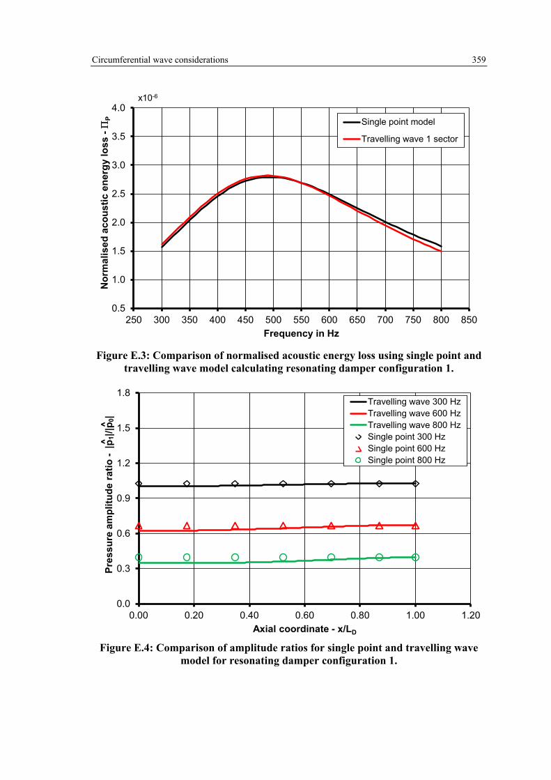
Circumferential wave considerations 359
0.5
1.0
1.5
2.0
2.5
3.0
3.5
4.0
250 300 350 400 450 500 550 600 650 700 750 800 850
Nor
mal
ised
aco
ustic
ene
rgy
loss
-Π
P
Frequency in Hz
Single point model
Travelling wave 1 sector
x10-6
Figure E.3: Comparison of normalised acoustic energy loss using single point and
travelling wave model calculating resonating damper configuration 1.
0.0
0.3
0.6
0.9
1.2
1.5
1.8
0.00 0.20 0.40 0.60 0.80 1.00 1.20Axial coordinate - x/LD
Travelling wave 300 HzTravelling wave 600 HzTravelling wave 800 HzSingle point 300 HzSingle point 600 HzSingle point 800 Hz
Pres
sure
am
plitu
de ra
tio -
|p1|/
|p0|
^^
Figure E.4: Comparison of amplitude ratios for single point and travelling wave
model for resonating damper configuration 1.

Circumferential wave considerations 360
-180
-120
-60
0
60
120
180
0.0 0.2 0.4 0.6 0.8 1.0 1.2
Phas
e di
ffere
nce
in d
egre
es
Axial coordinate - x/LD
Travelling wave 300 HzTravelling wave 600 HzTravelling wave 800 HzSingle point 300 HzSingle point 600 HzSingle point 800 Hz
Figure E.5: Comparison of phase difference between excitation amplitude and cav-
ity amplitude for single point and travelling wave model calculating resonating damper configuration 1.
-240
-210
-180
-150
-120
-90
-60
-30
0
0.0 0.2 0.4 0.6 0.8 1.0 1.2
Phas
e of
cav
ity p
ress
ure
wav
e in
deg
rees
Axial coordinate - x/LD
300 Hz600 Hz800 Hz
Figure E.6: Comparison of phase angle of cavity pressure wave calculated by trav-
elling wave model for resonating damper configuration 1.

Circumferential wave considerations 361
0.0
2.0
4.0
6.0
8.0
10.0
12.0
14.0
250 300 350 400 450 500 550 600 650 700 750 800 850
Nor
mal
ised
aco
ustic
ene
rgy
loss
-Π
P
Frequency in Hz
Two single sector dampersOne damper two sectors wideThree single sector dampersOne damper three sectors wide
x10-6
Figure E.7: Variation of damper length compared to multiple single sector damper
configurations.
0
20
40
60
80
100
120
140
160
0.0 0.2 0.4 0.6 0.8 1.0 1.2
Cav
ity p
ress
ure
ampl
itude
in P
a pk
Axial coordinate - x/LD Figure E.8: Half wave mode shape in damper cavity volume at 720 Hz for three
sector calculation.

Circumferential wave considerations 362
-180
-120
-60
0
60
120
180
0.0 0.2 0.4 0.6 0.8 1.0 1.2
Phas
e w
ithin
dam
per c
avity
in d
egre
es
Axial coordinate - x/LD Figure E.9: Phase of half wave mode shape in damper cavity volume at 720 Hz for
three sector calculation.