Proceedings, Bicycle and Motorcycle Dynamics 2010Symposium on the Dynamics and Control of Single Track Vehicles,

20–22 October 2010, Delft, The Netherlands

Accurate Measurement of Bicycle Parameters

Jason K. Moore∗, Mont Hubbard∗, A. L. Schwab†, J. D. G. Kooijman†

∗ Department of Mechanical and Aerospace EngineeringUniversity of California, Davis

One Shields Avenue, Davis, CA, 95616, USAe-mail: jkmoor@ucdavis.edu, mhubbard@ucdavis.edu

† Laboratory for Engineering MechanicsDelft University of Technology

Mekelweg 2, 2628CD Delft, The Netherlandse-mail: a.l.schwab@tudelft.nl, jodikooijman@gmail.com

ABSTRACT

Accurate measurements of a bicycle’s physical parameters are required for realistic dynamic sim-ulations and analysis. The most basic models require the geometry, mass, mass location and massdistributions for the rigid bodies. More complex models require estimates of tire characteristics,human characteristics, friction, stiffness, damping, etc. In this paper we present the measurementof the minimal bicycle parameters required for the benchmark Whipple bicycle model presentedin [7]. This model is composed of four rigid bodies, has ideal rolling and frictionless joints, and islaterally symmetric. A set of 25 parameters describes the geometry, mass, mass location and massdistribution of each of the rigid bodies. The experimental methods used to estimate the parametersdescribed herein are based primarily on the work done in [3] but have been refined for improvedaccuracy and methodology. Koojiman’s work was preceded by [10] who measured a bicycle in asimilar fashion and both [1] and [12] who used similar techniques with scooters.

We measured the physical characteristics of six different bicycles, two of which were set up intwo different configurations. The six bicycles, chosen for both variety and convenience, are asfollows: Batavus Browser, a Dutch style city bicycle measured with and without instrumentationas described in [6]; Batavus Stratos Deluxe, a Dutch style sporty city bicycle; Batavus CrescendoDeluxe a Dutch style city bicycle with a suspended fork; Gary Fisher Mountain Bike, a hardtailmountain bicycle; Bianchi Pista, a modern steel frame track racing bicycle; and Yellow Bicycle, astripped down aluminum frame road bicycle measured in two configurations, the second with thefork rotated in the headtube 180 degrees for larger trail.

These eight different parameter sets can be used with, but are not limited to, the benchmark bicyclemodel. The accuracy of all the measurements are presented up through the eigenvalue predictionof the linear model. The accuracies are based on error propagation theory with correlations takeninto account.

Keywords: bicycle, parameters, eigenvalues, Bode.

1 INTRODUCTION

This work is intended to document the indirect measurement of eight real bicycles’ physical pa-rameters. The physical parameters measured are those needed for the benchmark Whipple bicycle

model presented in [7]. The work is based on techniques used to measure the instrumented bi-cycles in [3], [5] and [8]. We improve upon these methods by both increasing and reporting theaccuracies of the measurements and by measuring the complete moments of inertia of the frameand fork needed for analysis of the nonlinear model. Furthermore, very little data exists on thephysical parameters of different types of bicycles and this work aims to provide a small sample ofbicycles.

Döhring [1] and Singh and Goel [12] measured the physical parameters of scooters. Roland andMassing [10] measured the physical parameters of a bicycle in much the same way as is presented,including calculations of uncertainty from the indirect measurement techniques. Patterson [9] useda swing to measure the inertia of a bicycle and rider. The present work is based on the work doneby Kooijman [3] using much of the same apparatus and refining the measurement technique.

2 BENCHMARK BICYCLE MODEL

Recently, the Whipple bicycle model has been benchmarked [7] and this model is widely used forbicycle dynamics studies. The unforced two degree-of-freedom, q = [steer and roll], model takesthe form:

Mq + vC1q +[gK0 + v2K2

]q = 0 (1)

where the entries of the M, C1, K0 and K2 matrices are combinations of 25 bicycle physicalparameters that include the geometry, mass, mass location and mass distribution of the four rigidbodies. The 25 parameters presented in [7] are not necessarily a minimum set for the Whipplemodel, as shown in [11], but are useful as they represent more intuitively measurable quantities.Furthermore, many more parameters are not needed due to the assumptions of the Whipple modelsuch as no-slip tires, lateral symmetry, knife edge wheels, etc.

3 BICYCLE DESCRIPTIONS

We choose to measure the physical parameters of six bicycles Fig. 1. The three Batavus bicycleswere donated by the manufacturer. We asked for a bicycle that they considered stable and one thatthey did not. They claimed the Browser was a “stable” bicycle and that the Stratos was “nervous”.The Fisher and the Pista were chosen to provide some variety, a mountain and road bike. Theyellow bike is used to demonstrate bicycle stability.

Batavus Browser (B, B*) The Batavus Browser Fig. 1a is an average priced Dutch city bike.It has a steel frame, a three speed internal rear hub, handle bars for an upright postureand includes various accessories for utility purposes. We measured the physical proprietiesof the stock Browser model and also equipped with the instrumentation used in our otherexperiments [4].

Batavus Crescendo Deluxe (C) The Batavus Crescendo Deluxe Fig. 1b is also a Dutch city bikefor touring. It has an aluminum frame, an eight speed internal hub, upright handlebars,accessories for utility and a suspension fork and suspension seatpost.

Gary Fisher Ziggurat (G) The Gary Fisher Ziggurat Fig. 1c is a modern lightweight front sus-pended mountain bike. It has a aluminum frame, large low pressure mountain bike tires, andis for racing with few extra accessories.

2

(a) Batavus Browser (b) Batavus Crescendo Deluxe (c) Gary Fisher

(d) Bianchi Pista (e) Batavus Stratos Deluxe (f) Yellow Bicycle

Figure 1: The six bicycles measured in the experiments. The Batavus Browser (a) is shown withthe instrumentation and the Yellow Bicycle (f) is shown with its fork reversed.

Bianchi Pista (P) The Bianchi Pista Fig. 1d is a modern lightweight steel track bicycle. It has asingle gear ratio and minimal extras to keep the weight low. It has drop handlebars and highpressure racing tires.

Batavus Stratos Deluxe (S) The Batavus Stratos Deluxe Fig. 1e is a sporty Dutch city bicycle.The frame is aluminum. It has a seven-speed internal hub and mountain style handle barsfor a less upright seating posture, but also includes accessories for utility such as a rear rack,fenders, light and chainguard.

Yellow Bicycle (Y, Y*) The yellow bicycle Fig. 1f is used in the lab to demonstrate that a bicycleis stable at certain speeds. It is an aluminum road frame of unknown make with the mostof components removed. The wheels, drop handlebar, seat, seat post and bottom bracketare the only parts on the bike. This bicycle was measured with both the fork in normalposition and reversed. The fork was reversed to ”decrease the minimal stable speed“ [3] ofthe bicycle.

4 PARAMETERS

The 25 parameters can be estimated using many techniques. Where possible we measured thebenchmark parameter directly.

5 ACCURACY

We took great care to improve and report the accuracy of the measurements of the parameters.Following the thrust of [10] we used error propagation theory to calculate accuracy of the 25benchmark parameters. We start by estimating the standard deviation of the actual measurements

3

Figure 2: Wheel and tire with chalk mark aligned to the tape measure.

taken. If x is a parameter and is a function of the measurements, u, v, . . ., then x is a randomvariable defined as x = f(u, v, . . .). The sample variance of x is defined as

s2x =1

N − 1

N∑i=1

[(ui − u)2

(∂x

∂u

)2

+ (vi − v)2(∂x

∂v

)2

+ 2(ui − u)(vi − v)

(∂x

∂u

)(∂x

∂v

)+ . . .

](2)

Using the definitions for variance and covariance, Equation 2 can be simplified to

s2x = s2u

(∂x

∂u

)2

+ s2v

(∂x

∂v

)2

+ 2suv

(∂x

∂u

)(∂x

∂v

)+ . . . (3)

If u and v are uncorrelated then suv = 0. Most of the calculations hereafter have uncorrelatedvariables but a few do not and the covariance has to be taken into account. Equation 3 can be usedto calculated the variance of all types of functions. Simple addition of two random variables maybe the most basic example:

x = au+ bv (4)

sx = a2s2u + b2s2v (5)

6 GEOMETRY

6.1 WHEEL RADII

The radii of the front rF and rear rR wheels were estimated by measuring the linear distance tra-versed along the ground through either 13 or 14 rotations of the wheel. Each wheel was measuredseparately and the measurements were taken with a 72kg rider seated on the bicycle. A 30 metertape measure (resolution: 2mm) was pulled tight and taped on a flat level smooth floor. The tirewas marked with chalk and aligned with the tape measure Fig. 2. The accuracy of the distancemeasurement is approximately ±0.01m. The tires were pumped to the recommended inflationpressure before the measurements. The wheel radius is calculated by

r ± σr =d

2πn±( σd

2πn

)(6)

4

6.2 HEAD TUBE ANGLE

The head tube angle was measured directly using an electronic level with a ±0.2◦ accuracy. Thebicycle frame was fixed perpendicular to the ground, the steering angle was set to the nominal, tirepressures were at recommended levels and the bicycle was unloaded. The steer axis tilt λ is thecomplement to the head tube angle.

λ± σλ =π

180◦(90◦ − λht) ±

( π

180◦

)σλht (7)

6.3 TRAIL

Trail is difficult to measure directly so we instead chose to measure the fork offset. The fork offsetwas measured by clamping the steer tube of the front fork into a v-block on a flat table. A rulerwas used to measure the height of the center of the head tube and the height of the center of theaxle axis. The fork blades were aligned such that the axle axis was parallel to the table surface.

c =rF sinλ− fo

cosλ(8)

σ2c = σ2rF tan2 λ− σ2fo sec2 λ+ σ2λ(rF sec2 λ− fo secλ tanλ

)2 (9)

6.4 WHEELBASE

We measured the wheelbase with the bicycle in nominal configuration described in Sec. 6.2. Weused a tape measure to measure the distance from one wheel axle center to the other with a 0.002m accuracy.

7 MASS

The total mass of each bicycle was measured using a spring scale with a resolution of 100 grams.The total mass was only used for comparison purposes. Each of the four bicycle parts were mea-sured using a Molen 20 kilogram scale with a resolution of 20 grams. The accuracy was conser-vatively assumed to also be ±20 grams.

8 CENTER OF MASS

8.1 WHEELS

The centers of mass of the wheels are assumed to be at their geometrical centers to comply withthe Whipple model.

8.2 REAR FRAME

The rear frame was hung in three orientations as a torsional pendulum (both for the center of massmeasurements and the moment of inertia measurements described in Sec. 9). We assumed thatthe frame was laterally symmetric, complying with the Whipple model. The frame could rotateabout a joint such that gravity aligned the center of mass with the pendulum axis. The orientationangle of the headtube, αB, Fig. 4a relative to the earth was measured using a digital level (±0.2◦

accuracy), Figure 5a. A string was aligned with the pendulum axis and allowed to pass by the

5

Figure 3: The scale used to measure the mass of each bicycle component.

frame. The horizontal distance aB between the rear axle and the string was measured by aligninga ruler perpendicular to the string. The distance aB was negative if the string fell to the right ofthe rear axle and positive if it fell to the left of the rear axle. These measurements allow for thecalculation of the center of mass location in the global reference frame. The frame rotation angleβB is defined as rotation of the frame in the nominal configuration to the hanging orientation,rotated about the Y axis.

β = λ− α (10)

σ2β = σ2λ + σ2α (11)

The center of mass can be found by realizing that the pendulum axis XP is simply a line inthe nominal bicycle reference frame with a slope m and a z-intercept b where the i subscriptcorresponds the different frame orientations Fig. 4b. The slope can be shown to be

mi = − tanβi (12)

σ2m = σ2β sec4 β (13)

The z-intercept can be shown to be

bi = −(

aBcosβi

+ rR

)(14)

σ2b = σ2a sec2 β + σ2rR + σ2βa2 sec2 β tan2 β (15)

Theoretically, the center of mass lies on each line but due to experimental error, if there are morethan two lines, the lines do not cross all at the same point. Only two lines are required to calculatethe center of mass of the laterally symmetric frame, but more orientations increase the center ofmass measurement accuracy. The three lines are defined as:

z = mix+ bi (16)

6

(a) (b)

Figure 4: (a) Pictorial description of the angles and dimensions that related the nominal bicyclereference frame XY ZB with the pendulum reference frame XY ZP . (b) Exaggerated intersectionof the three pendulum axes and the location of the center of mass.

The mass center location can be calculated by finding the intersection of these three lines. Twoapproaches were used used to calculate the center of mass. Intuition lead us to think that the centerof mass is located at the centroid of the triangle made by the three intersecting lines. The centroidcan be found by calculating the intersection point of each pair of lines and then averaging the threeintersection points. [

−m1 1−m2 1

] [xaza

]=

[b1b2

](17)

xB =xa + xb + xc

3(18)

zB =za + zb + zc

3(19)

Alternatively, the three lines can be treated as an over determined linear system and the leastsquares method is used to find a unique solution. This solution is not the same as the trianglecentroid method. −m1 1

−m2 1−m3 1

[ xBzB

]=

b1b2b3

(20)

The solution with the higher accuracy is the preferred one.

8.3 Fork

The fork and handlebars are a bit trickier to hang in three different orientations. Typically twoangles can be obtained by clamping to the steer tube at the top and the bottom. The third anglecan be obtained by clamping to the stem. The center of mass of the fork is calculated in the samefashion. The slope of the line in the benchmark reference frame is the same as for the frame butthe z-intercept is different:

b = w tanβ − rF − a

cosβ(21)

7

(a) (b)

Figure 5: (a) The digital level was mounted to a straight edge aligned with the headtube of thebicycle frame. This was done without allowing the straight edge to touch the frame. The framewasn’t completely stationary so this was difficult. The light frame oscillations could be damped outby submerging a low hanging area of the frame into a bucket of water to decrease the oscillation.(b) Measuring the distance from the pendulum axis to the rear wheel axle using level ruler.

σ2b = σ2w tan2 β + σ2β(w sec2 β − a secβ tanβ

)2+ σ2rF + σ2a sec2 β (22)

9 MOMENT OF INERTIA

The moments of inertia of the wheels, frame and fork were measured by taking advantage of the as-sumed symmetry of the parts and by hanging the parts as both compound and torsional pendulumsand measuring their periods of oscillation when perturbed at small angles. The rate of oscillationwas measured using a Silicon Sensing CRS03 100 deg/s rate gyro. The rate gyro was sampledat 1000hz with a National Instruments USB-6008 12 bit data acquisition unit and MATLAB. Themeasurement durations were either 15 or 30 secs and each moment of inertia measurement wasperformed three times. No extra care was taken to calibrate the rate gyro, maintain a constantpower source (i.e. the battery drains slowly), or account for drift. The raw voltage signal wasused to determine only the period of oscillation which is needed for the moment of inertia calcu-lations. The function Eqn 23 was fit to the data using a nonlinear least squares fit routine for eachexperiment to determine the quantities A, B, C, ζ, and ω.

f(t) = A+ e−ζωt[B sin

√1 − ζ2ωt+ C cos

√1 − ζ2ωt

](23)

Most of the data fit the damped oscillation function well with very light (and ignorable) damping.There were several instances of beating-like phenomena for some of the parts at particular orien-tations. Roland and Massing [10] also encountered this problem and used a bearing to prevent thetorsional pendulum from swinging. Figure 7 shows an example of the beating like phenomena.

The physical phenomenon observed corresponding to data sets such as these was that the bicycleframe or fork was perturbed torsionally. After set into motion the torsional motion died out anda longitudinal swinging motion increased. The motions alternated back and forth with neitherever reaching zero. The frequencies of these motions were very close to one another and it is not

8

Figure 6: Example of the raw voltage data taken during a 30 second measurement of the oscillationof one of the components.

Figure 7: An example of the beating-like phenomena observed on 5% of the experiments.

apparent how dissect the two. We explored fitting to a function such as

f(t) = A sin (ω1t) +B sin (ω2t+ φ) + C (24)

But the fit predicts that ω1 and ω2 are very similar frequencies. There was no easy way to choosewhich of the two ω’s was the one associated with the torsional oscillation. Some work was doneto model the torsional pendulum as a laterally flexible beam to determine this, but we thoughtaccuracy of the period calculation would not improve enough for the effort required. Future exper-iments should simply prevent the swinging motion of the pendulum without damping the torsionalmotion.

The period for a damped oscillation is

T =2π√

1 − ζ2ωn(25)

9

Figure 8: The rigid pendulum fixture mounted to a concrete column.

The uncertainty in the period, T , can be determined from the fit. Firstly, the variance of the fit is

σ2y =1

N − 5

N∑i=1

(ymi − ym)2 − (ypi − ym)2 (26)

The covariance matrix of the fit function can be formed

U = σ2yH−1 (27)

where H is the Hessian [2]. U is a 5×5 matrix with the variances of each of the five fit parametersalong the diagonal. The variance of T can be computed using the variance of ζ and ω. It isimportant to note that the uncertainties in the period are very low (< 1e− 4), even for the fits withlow r2 values.

9.1 TORSIONAL PENDULUM

A torsional pendulum was used to measure all moments of inertia about axes in the laterally sym-metric plane of each of the wheels, fork and frame. The pendulum is made up of a rigid mount,an upper clamp, a torsion rod, and various lower clamps. A 5 mm diameter, 1 m long mild steelrod was used as the torsion spring. A lightweight, low relative moment of inertia clamp wasconstructed that could clamp the rim and the tire. The moments of inertia of the clamps wereneglected. The wheel was hung freely such that the center of mass aligned with the torsional pen-dulum axis and then secured. The wheel was then perturbed and oscillated about the pendulumaxis. The rate gyro was mounted on the clamp oriented along the pendulum axis.

The torsional pendulum was calibrated using a known moment of inertia Fig. 9. A torsionalpendulum almost identical to the one used in [3] was used to measure the average period T iof oscillation of the rear frame at three different orientation angles βi, where i = 1, 2, 3, as shownin Fig. 4b. The parts were perturbed lightly, less than 1 degree, and allowed to oscillate about thependulum axis through at least ten periods. This was done at least three times for each frame andthe recorded periods were averaged.

10

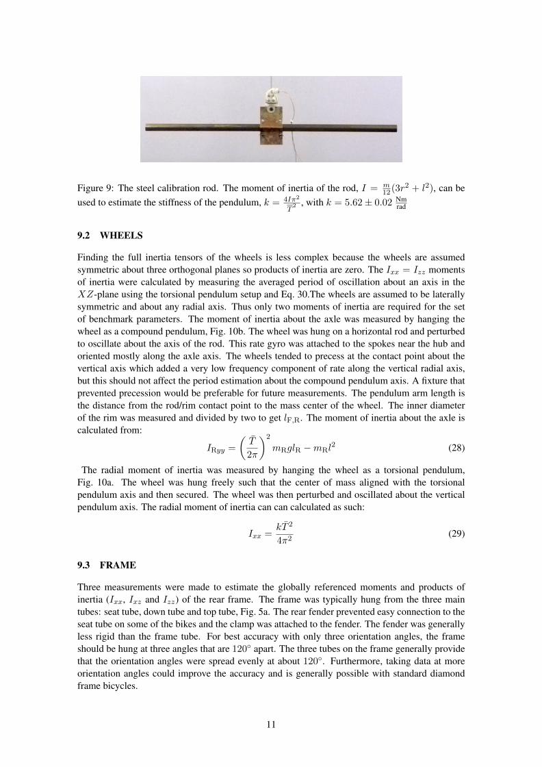
Figure 9: The steel calibration rod. The moment of inertia of the rod, I = m12(3r2 + l2), can be

used to estimate the stiffness of the pendulum, k = 4Iπ2

T2 , with k = 5.62 ± 0.02 Nm

rad

9.2 WHEELS

Finding the full inertia tensors of the wheels is less complex because the wheels are assumedsymmetric about three orthogonal planes so products of inertia are zero. The Ixx = Izz momentsof inertia were calculated by measuring the averaged period of oscillation about an axis in theXZ-plane using the torsional pendulum setup and Eq. 30.The wheels are assumed to be laterallysymmetric and about any radial axis. Thus only two moments of inertia are required for the setof benchmark parameters. The moment of inertia about the axle was measured by hanging thewheel as a compound pendulum, Fig. 10b. The wheel was hung on a horizontal rod and perturbedto oscillate about the axis of the rod. This rate gyro was attached to the spokes near the hub andoriented mostly along the axle axis. The wheels tended to precess at the contact point about thevertical axis which added a very low frequency component of rate along the vertical radial axis,but this should not affect the period estimation about the compound pendulum axis. A fixture thatprevented precession would be preferable for future measurements. The pendulum arm length isthe distance from the rod/rim contact point to the mass center of the wheel. The inner diameterof the rim was measured and divided by two to get lF,R. The moment of inertia about the axle iscalculated from:

IRyy =

(T

2π

)2

mRglR −mRl2 (28)

The radial moment of inertia was measured by hanging the wheel as a torsional pendulum,Fig. 10a. The wheel was hung freely such that the center of mass aligned with the torsionalpendulum axis and then secured. The wheel was then perturbed and oscillated about the verticalpendulum axis. The radial moment of inertia can can calculated as such:

Ixx =kT 2

4π2(29)

9.3 FRAME

Three measurements were made to estimate the globally referenced moments and products ofinertia (Ixx, Ixz and Izz) of the rear frame. The frame was typically hung from the three maintubes: seat tube, down tube and top tube, Fig. 5a. The rear fender prevented easy connection to theseat tube on some of the bikes and the clamp was attached to the fender. The fender was generallyless rigid than the frame tube. For best accuracy with only three orientation angles, the frameshould be hung at three angles that are 120◦ apart. The three tubes on the frame generally providethat the orientation angles were spread evenly at about 120◦. Furthermore, taking data at moreorientation angles could improve the accuracy and is generally possible with standard diamondframe bicycles.

11

(a) (b)

Figure 10: (a) The front wheel of the Crescendo hung as a torsional pendulum. (b) A wheel hungas a compound pendulum.

Three moments of inertia Ji about the pendulum axes were calculated using Eq. 30.

Ji =kT

2i

4π2(30)

The moments and products of inertia of the rear frame and handlebar/fork assembly with refer-ence to the benchmark coordinate system were calculated by formulating the relationship betweeninertial frames

Ji = RiIRTi (31)

where Ji is the inertia tensor about the pendulum axes, I, is the inertia tensor in the global referenceframe and R is the rotation matrix relating the two frames, Fig. 4a. The global inertia tensor isdefined as

I =

[Ixx IxzIxz Izz

]. (32)

The inertia tensor can be reduced to a 2 × 2 matrix because the frame is assumed to be laterallysymmetric and the y axis of the pendulum reference is the same as the y axis of the benchmarkreference frame. The simple rotation matrix about the Y -axis can similarly be reduced to a 2 × 2matrix where sβi and cβi are defined as sinβi and cosβi, respectively.

R =

[cβi −sβisβi cβi

](33)

The first entry of Ji in Eq. 31 is the moment of inertia about the pendulum axis and is writtenexplicitly as

Ji = c2βiIxx − 2sβicβiIxz + s2βiIzz . (34)

Similarly, calculating all three Ji allows one to form J1J2J3

=

c2β1 −2sβ1cβ1 s2β1c2β2 −2sβ2cβ2 s2β2c2β3 −2sβ3cβ3 s2β3

IxxIxzIzz

(35)

12

(a) (b)

Figure 11: (a) Rear frame hung as a compound pendulum. (b) Browser fork hung as a compoundpendulum.

and the moments of inertia can be solved for. The inertia of the frame about an axis normal tothe plane of symmetry was estimated by hanging the frame as a compound pendulum at the wheelaxis, Fig. 11a. Equation 28 is used but with the mass of the frame and the frame pendulum length.

lB =√x2B + (zB + rR)2 (36)

9.4 FORK AND HANDLEBAR

The inertia of the fork and handlebar is calculated in the same way as the frame. The fork is hungas both a torsional pendulum, Fig. 12, and as a compound pendulum, Fig. 11b. The fork providesfewer mounting options to obtain at least three equally spaced orientation angles, especially ifthere is no fender. The torsional calculations follow equations 30 through 35 and the compoundpendulum calculations is calculated with equation 28. The fork pendulum length is calculatedusing

lH =√

(xH − w)2 + (zB + rF )2 (37)

10 LINEAR ANALYSIS

Once all bicycle parameters have been calculated the canonical matrices can be formed and thelinear dynamics of the bicycles can be explored. The values of the canonical matrices can be foundin the second table in Appendix A. We also added the same rigid rider to each bicycle for further

13

Figure 12: The Stratos fork and handlebar assembly hung as a torsional pendulum.

Table 1: Mass, center of mass and moment of inertia for the rider relative to the benchmarkcoordinate system from [8]

Parameter ValuemP [kg] 72xP [m] 0.2909zP [m] -1.1091

IP [kg m2]

7.9985 0 −1.92720 8.0689 0

−1.9272 0 2.3624

comparison. The rigid rider was assumed to be in the same position and posture for each bicyclerelative to the rear wheel contact point.

10.1 EIGENVALUES

The eigenvalues of the bicycles with (Fig. 13) and without (Fig. 16 the rider can be plotted versusforward speed. Figure 13 shows that the bikes have the typical characteristics of the benchmarkbicycle: four real roots at very slow speeds, two of which are unstable; a complex pair that isunstable at lower speeds and stable at intermediate speeds; and a root that is mildly unstable athigher speeds. The one noticeable difference is that the capsize and caster modes are containedin a complex pair between about 0.5 and 3 m/s. The frequency of oscillation is of comparablemagnitude to that of the weave mode. But, the root locus in the real and imaginary plane, Fig. 14,shows that the mode damps out quickly. Examining the eigenvectors reveals that the mode is steerleading roll with a 90 degree phase, both of their magnitudes being similar, Fig 15. With the rideradded, the second complex pair disappears and the bikes have the typical characteristics of thebenchmark bicycle model. Reversing the fork on the yellow bike lowers the weave critical speedand increases the stable speed range. Also, the addition of weight to the rear rack of the Browserdoes little to the eigenvalues.

10.2 FREQUENCY RESPONSE

The frequency response of the bicycles (Fig. 17) and bicycle with rider (Fig. 18) also reveal someinteresting things. In the steer-torque-to-roll Bode diagram the magnitude difference among bi-cycles can vary up to 10 dB (or about 8.5 degrees per Newton-meter of torque) for the particularspeed shown. The difference in the frequency response for the bicycle with the rigid rider shows

14

0 2 4 6 8 10Speed [m/s]

10

5

0

5

10Re

al a

nd Im

agin

ary

Part

s of

the

Eige

nval

ue [1

/s] Bike Eigenvalues vs Speed

Batavus BrowserBatavus Browser InstrumentedBatavus Crescendo DeluxeGary FisherBianchi PistaBatavus Stratos DeluxeYellow BikeYellow Bike Reversed Fork

Figure 13: Eigenvalues versus speed for all eight bicycles without the rider.

less variation among the bicycles, Fig. 18, as the rider’s mass and inertia play a larger roll.

11 CONCLUSION

We have presented a detailed method to accurately estimate the physical parameters of a bicycleneeded for the benchmarked Whipple bicycle model [7]. We measured eight different bicyclesproviding both the parameter sets and linear model coefficient matrices for the bicycles alone andthe bicycles with the same rigid rider. The uncertainties in the parameters and matrix coefficientsare included for the bicycle alone. Finally, we have presented a brief comparison of the eightbicycles using eigenanalysis and Bode frequency response.

12 ACKNOWLEDGEMENTS

This material is based upon work partially supported by the National Science Foundation underGrant No. 0928339.

REFERENCES

[1] DÖHRING, E. Über die Stabilität und die Lenkkräfte von Einspurfahrzeugen. PhD thesis,Technical University Braunschweig, Germany, 1953.

[2] HUBBARD, M., AND ALAWAYS, L. W. Rapid and accurate estimation of release conditionsin the javelin throw. Journal of Biomechanics 22 (1989), 583–595.

[3] KOOIJMAN, J. D. G. Experimental Validation of a Model for the Motion of an UncontrolledBicycle. MSc thesis, Delft University of Technology, 2006.

15

30 20 10 0 1015

10

5

0

5

10

15

Batavus Crescendo DeluxeEigenvalues vs Speed

0

1

2

3

4

5

6

7

8

9

10

Figure 14: The root loci with speed as the parameter for the Crescendo.

[4] KOOIJMAN, J. D. G., AND SCHWAB, A. L. Experimental validation of the lateral dynamicsof a bicycle on a treadmill. In Proceedings of the ASME 2009 International Design Engi-neering Technical Conferences & Computers and Information in Engineering Conference,IDETC/CIE 2009 (2009), no. DETC2009-86965.

[5] KOOIJMAN, J. D. G., SCHWAB, A. L., AND MEIJAARD, J. P. Experimental validation of amodel of an uncontrolled bicycle. Multibody System Dynamics 19 (May 2008), 115–132.

[6] KOOIJMAN, J. D. G., SCHWAB, A. L., AND MOORE, J. K. Some observations on humancontrol of a bicycle. In Proceedings of the ASME 2009 International Design and EngineeringTechnical Conferences & Computers and Information in Engineering Conference (2009).

0.4 0.2 0.0 0.2 0.4 0.6 0.8 1.0Real

0.2

0.1

0.0

0.1

0.2

0.3

0.4

0.5

Imag

inar

y

v=1.001 m/s, λ=−3.83 +0.48j

Roll RateSteer RateRoll AngleSteer Angle

Figure 15: Eigenvector components for the second complex mode pair at low speed.

16

0 2 4 6 8 10Speed [m/s]

10

5

0

5

10

Real

and

Imag

inar

y Pa

rts

of th

e Ei

genv

alue

[1/s

] Bike+Rider Eigenvalues vs Speed

Batavus BrowserBatavus Browser InstrumentedBatavus Crescendo DeluxeGary FisherBianchi PistaBatavus Stratos DeluxeYellow BikeYellow Bike Reversed Fork

Figure 16: Eigenvalues versus speed for all eight bicycles with the same rigid rider.

100806040200

Mag

nitu

de [d

B]

Bike Tδ/φ @ 2 m/s

100 101 102

Frequency [rad/s]

160140120100

806040200

Phas

e [d

eg]

Batavus BrowserBatavus Browser InstrumentedBatavus Crescendo DeluxeGary FisherBianchi PistaBatavus Stratos DeluxeYellow BikeYellow Bike Reversed Fork

Figure 17: The frequency response for steer-torque-to-roll for all eight bicycles without the riderat 2 m/s.

17

110100

9080706050403020

Mag

nitu

de [d

B]

Bike+Rider Tδ/φ @ 2 m/s

100 101 102

Frequency [rad/s]

180160140120100

806040200

Phas

e [d

eg]

Batavus BrowserBatavus Browser InstrumentedBatavus Crescendo DeluxeGary FisherBianchi PistaBatavus Stratos DeluxeYellow BikeYellow Bike Reversed Fork

Figure 18: The frequency response for steer-torque-to-roll for all eight bicycles with the same rigidrider at 2 m/s.

[7] MEIJAARD, J. P., PAPADOPOULOS, J. M., RUINA, A., AND SCHWAB, A. L. Linearizeddynamics equations for the balance and steer of a bicycle: A benchmark and review. Pro-ceedings of the Royal Society A: Mathematical, Physical and Engineering Sciences 463,2084 (Aug 2007), 1955–1982.

[8] MOORE, J. K., KOOIJMAN, J. D. G., HUBBARD, M., AND SCHWAB, A. L. A Methodfor Estimating Physical Properties of a Combined Bicycle and Rider. In Proceedings ofthe ASME 2009 International Design Engineering Technical Conferences & Computers andInformation in Engineering Conference, IDETC/CIE 2009 (San Diego, CA, USA, August–September 2009), ASME.

[9] PATTERSON, W. B. The Lords of the Chainring. W. B. Patterson, 2004.

[10] ROLAND JR., R. D., AND MASSING, D. E. A digital computer simulation of bicycle dy-namics. Calspan Report YA-3063-K-1, Cornell Aeronautical Laboratory, Inc., Buffalo, NY,14221, Jun 1971. Prepared for Schwinn Bicycle Company, Chicago, IL 60639.

[11] SHARP, R. S. Dynamical Analysis of Vehicle Systems, vol. 497 of CISM International Centrefor Mechanical Sciences. Springer Vienna, 2008, ch. Dynamics of Motorcycles: Stability andControl, pp. 183–230.

[12] SINGH, D. V., AND GOEL, V. K. Stability of Rajdoot Scooter. Tech. rep., SAE, 1971. SAEPaper 710273.

18

A PARAMETER TABLES

The tabulated values for the both the physical parameters and the canonical matrix coefficients areshown in the following four tables. The uncertainties in the estimations of both the parameters andcoefficients are also shown for the bicycle without a rider.

19

Table 2: The parameters for the eight bicycles with uncertainties in the estimations.

B B* C G P S Y Y*Parameter Value σ Value σ Value σ Value σ Value σ Value σ Value σ Value σw [m] 1.121 0.002 1.121 0.002 1.101 0.002 1.070 0.002 0.989 0.002 1.037 0.002 1.089 0.002 0.985 0.002c [m] 0.069 0.002 0.068 0.002 0.083 0.002 0.072 0.002 0.062 0.002 0.056 0.002 0.047 0.002 0.180 0.002λ [rad] 0.400 0.003 0.400 0.003 0.367 0.003 0.330 0.003 0.276 0.003 0.295 0.003 0.302 0.003 0.339 0.003rR [m] 0.3410 0.0001 0.3408 0.0001 0.3400 0.0001 0.3386 0.0001 0.3321 0.0001 0.3385 0.0001 0.3414 0.0001 0.3414 0.0001mR [kg] 3.11 0.02 3.11 0.02 3.96 0.02 1.94 0.02 1.38 0.02 3.96 0.02 2.57 0.02 2.57 0.02IRxx [kg m2] 0.0904 0.0004 0.0904 0.0004 0.0966 0.0004 0.0630 0.0003 0.0552 0.0002 0.0939 0.0004 0.0877 0.0004 0.0877 0.0004IRyy [kg m2] 0.152 0.001 0.152 0.001 0.144 0.001 0.101 0.001 0.076 0.001 0.154 0.001 0.149 0.001 0.149 0.001xB [m] 0.276 0.003 0.217 0.003 0.312 0.003 0.367 0.002 0.38 0.02 0.326 0.003 0.422 0.004 0.412 0.004zB [m] -0.538 0.003 -0.622 0.003 -0.526 0.003 -0.499 0.003 -0.477 0.007 -0.483 0.003 -0.603 0.004 -0.618 0.004mB [kg] 9.86 0.02 14.71 0.02 9.18 0.02 4.48 0.02 4.49 0.02 7.22 0.02 3.31 0.02 3.31 0.02IBxx [kg m2] 0.527 0.002 0.866 0.005 0.500 0.002 0.283 0.001 0.290 0.002 0.373 0.002 0.2240 0.0009 0.2253 0.0009IBxz [kg m2] -0.114 0.001 -0.181 0.004 -0.015 0.001 0.0559 0.0003 0.050 0.001 -0.0383 0.0004 0.0183 0.0001 0.0179 0.0001IByy [kg m2] 1.317 0.003 2.405 0.005 1.118 0.003 0.470 0.003 0.476 0.009 0.717 0.003 0.388 0.004 0.388 0.004IBzz [kg m2] 0.759 0.003 1.867 0.008 0.739 0.003 0.268 0.001 0.249 0.001 0.455 0.002 0.2164 0.0009 0.2150 0.0009xH [m] 0.867 0.004 0.867 0.004 0.907 0.005 0.960 0.006 0.906 0.005 0.911 0.004 0.948 0.004 0.919 0.005zH [m] -0.748 0.003 -0.747 0.003 -0.803 0.003 -0.719 0.004 -0.732 0.002 -0.73 0.002 -0.788 0.002 -0.816 0.002mH [kg] 3.22 0.02 3.22 0.02 4.57 0.02 2.52 0.02 2.27 0.02 3.04 0.02 2.45 0.02 2.45 0.02IHxx [kg m2] 0.253 0.001 0.253 0.001 0.387 0.002 0.115 0.001 0.0980 0.0004 0.1768 0.0008 0.1452 0.0006 0.1475 0.0006IHxz [kg m2] -0.072 0.0008 -0.072 0.0008 -0.076 0.001 -0.018 0.001 -0.0044 0.0003 -0.0273 0.0006 -0.0194 0.0005 -0.0172 0.0005IHyy [kg m2] 0.246 0.003 0.246 0.003 0.363 0.004 0.100 0.004 0.069 0.002 0.145 0.002 0.120 0.002 0.119 0.002IHzz [kg m2] 0.0956 0.0007 0.0956 0.0007 0.167 0.001 0.0227 0.0006 0.0396 0.0002 0.0446 0.0003 0.0292 0.0003 0.0294 0.0004rF [m] 0.3435 0.0001 0.3426 0.0001 0.3426 0.0001 0.3302 0.0001 0.3338 0.0001 0.3400 0.0001 0.3419 0.0001 0.3419 0.0001mF [kg] 2.02 0.02 2.02 0.02 3.55 0.02 1.50 0.02 1.58 0.02 3.33 0.02 1.90 0.02 1.90 0.02IFxx [kg m2] 0.0884 0.0004 0.0884 0.0004 0.0954 0.0004 0.0631 0.0003 0.0553 0.0002 0.0916 0.0004 0.0851 0.0003 0.0851 0.0003IFyy [kg m2] 0.149 0.001 0.149 0.001 0.166 0.001 0.106 0.001 0.106 0.001 0.157 0.001 0.147 0.002 0.147 0.002

20

Table 3: The canonical matrix coefficients for the eight bicycles with the uncertainty in the estimations.

B B* C G P S Y Y*Parameter Value σ Value σ Value σ Value σ Value σ Value σ Value σ Value σM11 6.21 0.03 9.39 0.06 7.44 0.04 3.33 0.02 3.07 0.03 4.88 0.02 3.79 0.02 3.96 0.02M12 0.33 0.01 0.36 0.01 0.69 0.02 0.37 0.01 0.33 0.01 0.41 0.01 0.33 0.01 0.68 0.01M21 0.33 0.01 0.36 0.01 0.69 0.02 0.37 0.01 0.33 0.01 0.41 0.01 0.33 0.01 0.68 0.01M22 0.220 0.002 0.223 0.002 0.373 0.006 0.152 0.005 0.155 0.003 0.203 0.003 0.165 0.003 0.301 0.006C111 0.0 NA 0.0 NA 0.0 NA 0.0 NA 0.0 NA 0.0 NA 0.0 NA 0.0 NAC112 4.39 0.03 4.97 0.04 6.45 0.04 3.44 0.02 3.44 0.04 4.85 0.03 3.63 0.02 4.70 0.03C121 -0.45 0.004 -0.451 0.004 -0.516 0.003 -0.344 0.004 -0.339 0.004 -0.489 0.003 -0.446 0.005 -0.554 0.005C122 0.58 0.01 0.63 0.01 1.11 0.03 0.57 0.02 0.55 0.01 0.75 0.02 0.52 0.01 1.05 0.02K011 -9.47 0.03 -13.31 0.05 -11.06 0.04 -5.2 0.03 -4.79 0.04 -8.18 0.03 -5.45 0.03 -5.57 0.03K012 -0.56 0.02 -0.59 0.02 -1.06 0.03 -0.57 0.02 -0.51 0.02 -0.71 0.02 -0.48 0.02 -0.94 0.02K021 -0.56 0.02 -0.59 0.02 -1.06 0.03 -0.57 0.02 -0.51 0.02 -0.71 0.02 -0.48 0.02 -0.94 0.02K022 -0.218 0.008 -0.228 0.008 -0.38 0.01 -0.185 0.007 -0.138 0.005 -0.206 0.007 -0.143 0.006 -0.311 0.008K211 0.0 NA 0.0 NA 0.0 NA 0.0 NA 0.0 NA 0.0 NA 0.0 NA 0.0 NAK212 8.50 0.03 11.67 0.05 10.14 0.04 5.15 0.03 5.19 0.04 8.39 0.03 5.54 0.03 6.16 0.03K221 0.0 NA 0.0 NA 0.0 NA 0.0 NA 0.0 NA 0.0 NA 0.0 NA 0.0 NAK222 0.60 0.02 0.62 0.02 1.05 0.03 0.60 0.02 0.58 0.02 0.78 0.02 0.53 0.01 1.03 0.02

21

Table 4: The parameters for the eight bicycles with the same rigid rider.

B B* C G P S Y Y*Parameter Value σ Value σ Value σ Value σ Value σ Value σ Value σ Value σw [m] 1.121 NA 1.121 NA 1.101 NA 1.07 NA 0.989 NA 1.037 NA 1.089 NA 0.985 NAc [m] 0.069 NA 0.068 NA 0.083 NA 0.072 NA 0.062 NA 0.056 NA 0.047 NA 0.18 NAλ [rad] 0.4 NA 0.4 NA 0.367 NA 0.33 NA 0.276 NA 0.295 NA 0.302 NA 0.339 NArR [m] 0.341 NA 0.341 NA 0.34 NA 0.339 NA 0.332 NA 0.338 NA 0.341 NA 0.341 NAmR [kg] 3.11 NA 3.11 NA 3.96 NA 1.94 NA 1.38 NA 3.96 NA 2.57 NA 2.57 NAIRxx [kg m2] 0.088 NA 0.088 NA 0.095 NA 0.063 NA 0.055 NA 0.092 NA 0.085 NA 0.085 NAIRyy [kg m2] 0.152 NA 0.152 NA 0.144 NA 0.101 NA 0.076 NA 0.154 NA 0.149 NA 0.149 NAxB [m] 0.289 NA 0.278 NA 0.293 NA 0.295 NA 0.296 NA 0.294 NA 0.297 NA 0.296 NAzB [m] -1.04 NA -1.027 NA -1.043 NA -1.073 NA -1.072 NA -1.052 NA -1.087 NA -1.088 NAmB [kg] 81.86 NA 86.71 NA 81.18 NA 76.48 NA 76.49 NA 79.22 NA 75.31 NA 75.31 NAIBxx [kg m2] 11.356 NA 11.759 NA 11.268 NA 9.851 NA 9.978 NA 10.947 NA 9.035 NA 8.988 NAIBxz [kg m2] -1.968 NA -1.67 NA -2.043 NA -2.067 NA -2.123 NA -2.111 NA -2.12 NA -2.098 NAIByy [kg m2] 12.218 NA 13.434 NA 11.96 NA 10.133 NA 10.271 NA 11.37 NA 9.324 NA 9.267 NAIBzz [kg m2] 3.124 NA 4.295 NA 3.105 NA 2.655 NA 2.648 NA 2.825 NA 2.633 NA 2.624 NAxH [m] 0.867 NA 0.867 NA 0.907 NA 0.96 NA 0.906 NA 0.911 NA 0.948 NA 0.919 NAzH [m] -0.748 NA -0.747 NA -0.803 NA -0.719 NA -0.732 NA -0.73 NA -0.788 NA -0.816 NAmH [kg] 3.22 NA 3.22 NA 4.57 NA 2.52 NA 2.27 NA 3.04 NA 2.45 NA 2.45 NAIHxx [kg m2] 0.253 NA 0.253 NA 0.387 NA 0.115 NA 0.098 NA 0.177 NA 0.145 NA 0.147 NAIHxz [kg m2] -0.072 NA -0.072 NA -0.076 NA -0.018 NA -0.004 NA -0.027 NA -0.019 NA -0.017 NAIHyy [kg m2] 0.246 NA 0.246 NA 0.363 NA 0.1 NA 0.069 NA 0.145 NA 0.12 NA 0.119 NAIHzz [kg m2] 0.096 NA 0.096 NA 0.167 NA 0.023 NA 0.04 NA 0.045 NA 0.029 NA 0.029 NArF [m] 0.344 NA 0.343 NA 0.343 NA 0.33 NA 0.334 NA 0.34 NA 0.342 NA 0.342 NAmF [kg] 2.02 NA 2.02 NA 3.545 NA 1.5 NA 1.58 NA 3.334 NA 1.9 NA 1.9 NAIFxx [kg m2] 0.09 NA 0.09 NA 0.097 NA 0.063 NA 0.055 NA 0.094 NA 0.088 NA 0.088 NAIFyy [kg m2] 0.149 NA 0.149 NA 0.166 NA 0.106 NA 0.106 NA 0.157 NA 0.147 NA 0.147 NA

22

Table 5: The canonical matrix coefficients for the eight bicycles with the rigid rider.

B B* C G P S Y Y*Parameter Value σ Value σ Value σ Value σ Value σ Value σ Value σ Value σM11 102.78 NA 105.957 NA 104.002 NA 99.894 NA 99.631 NA 101.443 NA 100.353 NA 100.529 NAM12 1.536 NA 1.552 NA 2.195 NA 1.731 NA 1.608 NA 1.515 NA 1.216 NA 4.354 NAM21 1.536 NA 1.552 NA 2.195 NA 1.731 NA 1.608 NA 1.515 NA 1.216 NA 4.354 NAM22 0.249 NA 0.251 NA 0.417 NA 0.187 NA 0.185 NA 0.229 NA 0.182 NA 0.557 NAC111 0.0 NA 0.0 NA 0.0 NA 0.0 NA 0.0 NA 0.0 NA 0.0 NA 0.0 NAC112 26.395 NA 26.953 NA 30.154 NA 27.386 NA 28.964 NA 28.654 NA 25.623 NA 38.883 NAC121 -0.45 NA -0.451 NA -0.516 NA -0.344 NA -0.339 NA -0.489 NA -0.446 NA -0.554 NAC122 1.037 NA 1.082 NA 1.722 NA 1.136 NA 1.118 NA 1.215 NA 0.868 NA 3.075 NAK011 -89.322 NA -93.167 NA -90.912 NA -85.055 NA -84.644 NA -88.034 NA -85.308 NA -85.427 NAK012 -1.742 NA -1.758 NA -2.539 NA -1.912 NA -1.766 NA -1.797 NA -1.35 NA -4.551 NAK021 -1.742 NA -1.758 NA -2.539 NA -1.912 NA -1.766 NA -1.797 NA -1.35 NA -4.551 NAK022 -0.678 NA -0.684 NA -0.91 NA -0.619 NA -0.481 NA -0.522 NA -0.401 NA -1.512 NAK211 0.0 NA 0.0 NA 0.0 NA 0.0 NA 0.0 NA 0.0 NA 0.0 NA 0.0 NAK212 74.125 NA 77.287 NA 77.857 NA 75.753 NA 82.885 NA 82.073 NA 75.55 NA 82.632 NAK221 0.0 NA 0.0 NA 0.0 NA 0.0 NA 0.0 NA 0.0 NA 0.0 NA 0.0 NAK222 1.57 NA 1.584 NA 2.3 NA 1.783 NA 1.802 NA 1.782 NA 1.295 NA 4.495 NA

23