accuracy of the spider model in decomposing layered surfaces
TRANSCRIPT

Accuracy of the Spider Model in Decomposing Layered Surfaces
Tetsuro MorimotoToppan Printing Co. Ltd.
Robby T. TanUtrecht UniversityThe Netherlands
Rei KawakamiThe University of Tokyo
Katsushi IkeuchiThe University of Tokyo
Abstract
The surface of most natural objects is composed oftwo or more layers whose optical properties jointly de-termine the surface’s overall reflectance. Light transmis-sion through these layers can be approximated by using theLambert-Beer (LB) model, which provides a good trade-offbetween the accuracy and simplicity to handle layer decom-position. Recently, a layer decomposition based on the LB-based model is proposed. Assuming surfaces with two lay-ers, it estimates the reflectance of top and bottom layers,as well as the opacity of the top layer. The method intro-duces the “spider model”, which is named after the colordistribution in the RGB space that resembles the shape ofspiders. In this paper, we intend to verify the accuracy ofthe spider model and the optical model where it is based on(i.e., the LB-based model). We verify the LB-based modelby comparing to the Kubelka-Munk (KM) model, which haspreviously been shown to be reliably accurate. The bene-fits of layer decomposition are easy to notice. First, manycomputer vision algorithms assume a single layer, and tendto fail when encountering multi-layered surfaces. Second,knowing the optical properties of each layer can providefurther knowledge of the target objects.
1. IntroductionIn computer vision, reflectance is conventionally as-
sumed to follow a single-layer reflection model, such asthe Lambertian model [16]. While this model can serve asan approximation of reflection of a single-layered surface,most objects in the real world, particularly natural ones,have surfaces that consist of multiple layers. For such ob-jects, single layer models often provide a poor representa-tion of their reflectance characteristics.
In multi-layered surfaces, each layer may have differentoptical parameter values. These values and the order of thelayers physically determine the reflectance of an object, andtherefore also the object’s appearance. For example, humanskin roughly consists of two layers, namely the dermis andepidermis [1], which both contribute to the unique appear-ance of skin. Other examples are plant leaves, biologicaltissues, and oxidized metals (patinas), paintings, etc.
Decomposing such surfaces, which means extractingeach layer optical properties, can benefit computer visionapplications and other fields, such as archeology, biology,medical image analysis, etc. Morimoto et al. [18] proposeda novel method that can extract the optical properties of lay-ered surfaces with two layers (i.e., top and bottom layers).The method extracts the opacity of the top layer and thereflection of both layers using the spider model. Given asingle input image containing one bottom layer and at leastone top layer, it fits the color distributions in the RGB spaceusing the spider model, and then estimates the optical pa-rameters.
The spider model proposed in [18] is a nonlinear equa-tion describing the correlation of the intensity values of lay-ered surfaces in the RGB space. It is called spider modelsince, when the intensity values of the mixtures of one bot-tom layer and n different top layers are projected onto thecolor space, then we will have n different curves intersect-ing at one point, resembling the shape of a spider. As dis-cussed in [18], the core of the spider model is the Lambert-Beer (LB) based model.
However, to our best knowledge, there are no discus-sion in the literature about the accuracy of the LB-basedmodel applied to layered surfaces and thus the spider model.Therefore, in this paper, our goal is to verify the accuracy ofthe two models. For verifying the LB-based model, we willcompare it with the Kubelka-Munk (KM) model, a two-flux
scattering model; while for the spider model, we will inves-tigate the differences of its generated RGB values from thecolor distributions of real data.
The fields of optics and color science have introducedmany models of multi-layered objects [5, 13]. These mod-els are principally based on radiative transfer theory [6].One highly detailed representation is the many-flux scat-tering model presented by Mudgett et al. [19]. Since thismodel has many parameters that make it difficult to apply,a simpler two-flux approximation called the Kubelka-Munk(KM) model [15] is practically more useful, particularly incolor science. Mudgett et al. [20] has theoretically verifiedthat the KM model works reliably (when the scattering co-efficient is relatively higher than the absorption coefficient);which is the main reason for us to use it as the standard forthe verification. Note that, while the KM model (which isa two-flux model) is considerably simpler than multi-fluxmodels, in computer vision, the model is still considerablycomplex, due to the highly nonlinear equation.
The KM model has been used to heighten the realism ofpigmented materials [11] and weathered objects [10]. It hasbeen frequently used in color matching of textiles, paints,printing inks and plastics (e.g., [9, 4]). Tsumura et al. [22]decomposed melanin and hemoglobin of human skin basedon the Lambert-Beer (LB) law [2] and later used the modelto generate skin colors under various values of melanin andhemoglobin concentrations [23]. Some researchers haveemployed the alpha matting equation for decomposing lay-ered scenes (e.g., [7, 17]). Since alpha matting utilizes alinear equation to model layer composition, it can be con-sidered as physically consistent with the LB law [21]. How-ever, most methods using the alpha matting equation as-sume the opacity to be independent from the wavelengths,which is different from the LB-based model [18]. In termsof the mathematical equation, the LB-based model is iden-tical to Koschmieder’s equation for radiance [14]; althoughto our knowledge, the equation has never been applied tolayered surfaces.
Organization The rest of this paper is organized as fol-lows. First, we review the layered surface decompositionusing the spider model in Section 2. In Section 3, we dis-cuss the two reflection models: the LB-based model andthe KM model, and compare them in Section 4. In Section5, we provide a discussion about the accuracy and effec-tiveness of the LB-based model, followed by conclusions inSection 6.
2. Layered Surface DecompositionMorimoto et al. [18] propose a layered-surface decom-
position method using the spider model. The method as-sumes two layers and estimates the following three opticalproperties: bottom layer’s reflection, top layer’s reflection
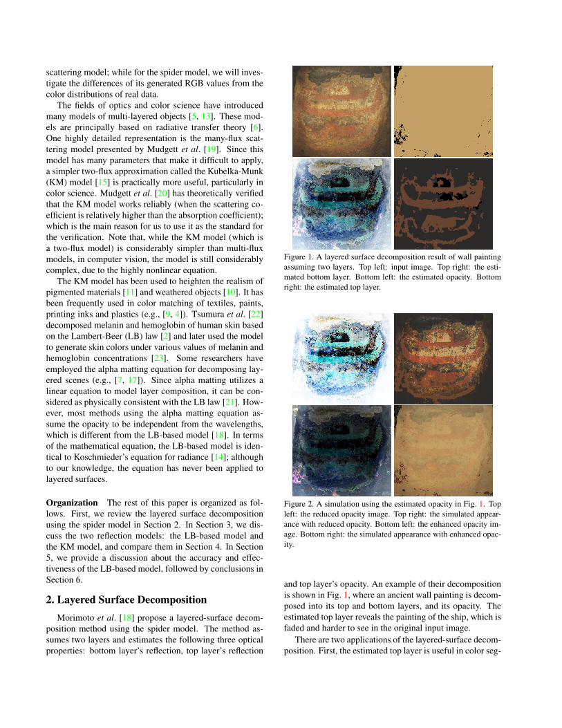
Figure 1. A layered surface decomposition result of wall paintingassuming two layers. Top left: input image. Top right: the esti-mated bottom layer. Bottom left: the estimated opacity. Bottomright: the estimated top layer.
Figure 2. A simulation using the estimated opacity in Fig. 1. Topleft: the reduced opacity image. Top right: the simulated appear-ance with reduced opacity. Bottom left: the enhanced opacity im-age. Bottom right: the simulated appearance with enhanced opac-ity.
and top layer’s opacity. An example of their decompositionis shown in Fig. 1, where an ancient wall painting is decom-posed into its top and bottom layers, and its opacity. Theestimated top layer reveals the painting of the ship, which isfaded and harder to see in the original input image.
There are two applications of the layered-surface decom-position. First, the estimated top layer is useful in color seg-

Figure 3. Spider model: Top row. Right: the generated image us-ing LB-based model. Left: we plotted three colors with variousopacity values into the RGB space. The gray circle represents thebottom layer’s reflection. Black circles represent the top layer’sreflection when the opacity=1. Each of the line follows the spi-der model in Eqs. (1) and (2). Bottom row. Left: the real image.Right: the plot of the left image into the RGB space. The gray cir-cle represents the bottom layer’s reflection. Black circles representthe top layer’s reflection with the largest opacity value.
mentation which normally suffers from color gradations oftop layers. Second, the three estimated properties are use-ful to simulate the synthetic appearance of a target object.Fig. 2 shows the results of changing the opacity. By eitherreducing or increasing the opacity, the image can fade outor become more salient.
Spider Model The spider model, which is the core in[18], is based on the Lambert-Beer law [2], and is math-ematically described as follows:
Ir = Br + ψr(Ig −Bg)γr , (1)Ib = Bb + ψb(Ig −Bg)γb , (2)
where Ic is the intensity of the input image (the mixed re-flection of layered surfaces), c is the index of the RGBcolor channels, Bc is the reflection of the bottom layer,Fc is the reflection of the top layer, γr = µr/µg , ψr =(Fr − Br)/(Fg − Bg)γr , ψb = (Fb − Bb)/(Fg − Bg)γb ,and γb = µb/µg , where µc is the attenuation factor of theLambert-Beer law. Each of the variables is dependent on x,the location of the pixel in the image.
The spider model is named after the shape of the plotof the model in a three-dimensional space (the space is notnecessarily composed of the RGB color channels, but anythree wavelengths with considerable distance among them).Due to the non-linear correlation between color channels
Figure 4. (a).The optical model of the Lambert-beer model.(b).The optical model based on the Lambert-Beer model of lay-ered surface objects
represented in Eqs. (1) and (2), the distribution forms acurve as depicted in Fig. 3. When multiple lines are ob-served, they resemble the shape of a spider. Each line startsat the color of the top layer with the largest opacity. Theopacity decreases along with the line. The end point repre-sents the bottom layer’s color where the opacity of the toplayer is equal to zero. By fitting the model to the observeddata, the optical parameters of the layered surface can beobtained.
3. Reflection Models3.1. Lambert-Beer based Model
Lambert-Beer Law [2] models the optical transmittanceof light passing through a transparent object:
T (λ) =Io(λ)Ii(λ)
= e−µ(λ)d, (3)
where T is the optical transmittance, λ is the wavelength, Iois the intensity of the outgoing light, Ii is the intensity of theincoming light, µ is the attenuation factor of the object, andd is the distance of the light traveling through the object.This law is illustrated in Fig. 4.a.
Based on the Lambert-Beer Law, the light reflected fromlayered surfaces can be modeled as:
Ic(x) = Bc(x)e−µc(x)d(x) + Fc(x)(1− e−µc(x)d(x)
), (4)
where index c represents one of the three color channels{r,g,b}. Ic is the mixture intensity of the transmitted lightfrom bottom and top layers. We call Ic a mixed layer.Bc and Fc are, respectively, the bottom and top layer’s re-flectance, when its thickness d is infinitely large. In thispaper, we define opacity φc = 1 − e−µcd. Finally, x is thespatial image coordinate, which for the sake of simplicity,we will omit throughout the paper. In the last equation, weassume that the camera’s color sensitivities follow the Diracdelta function. Although the model can be applied to spec-tral data, in this paper we focus on RGB images taken from

an ordinary digital camera whose gamma correction is setto off. Fig. 4.b illustrates the model.
Hence, if we have two-layered surfaces, they are com-posed of the bottom layer Bc, the top layer Fc, and theopacity of the top layer φ. In this paper, we assume thatthe opacity of the bottom layer is infinitely large throughoutthe input image, and also assume that the light coming onthe top layer is the same as that of the bottom layer. There-fore, based on the assumptions, we can calculate the mixedreflectance by canceling the incoming light intensity:
Rm = Rb
(1− φ
)+Rfφ, (5)
whereRm is the mixed reflectance, Rb is the bottom layer’sreflectance, and Rf is the top layer’s reflectance.
3.2. Kubelka-Munk Model
In this section, we provide a brief review of the KMmodel. For complete derivations and further details, read-ers are referred to [13, 24, 12]. Assuming we have a surfacecovered by a colorant as shown in Fig. 4.b, according to theKM model we can describe the mixed reflectanceRm of thesurface as:
Rm =1Rf
(Rb −Rf )−Rf (Rb − 1Rf
)eSd( 1
Rf−Rf )
(Rb −Rf )− (Rb − 1Rf
)eSd( 1
Rf−Rf )
,
(6)
where Rb is the bottom layer’s reflectance, Rf is the re-flectance of the top layer when its optical thickness (d) isinfinite, and S is the scattering coefficient of the foregroundlayer. All of these parameters except for d are dependent onwavelength. For most practical purposes, Sd can be treatedas a single quantity. Note thatRf andRb are conventionallydenoted asR∞ andRg , respectively; however, for clarity ofcomparison to related models, we employ our own notation.
The KM model offers some degree of physical accuracyin representing the reflectance of layered surfaces, but is for-mulated based on certain conditions [15, 4]: the layers con-tain colorants that scatter and absorb light (optically homo-geneous objects are excluded); the layer is flat and infinite;effects of polarization of light are ignored; the layer behavesas if the pigment particles are large with respect to the wave-length of light but very small compared to the thickness ofthe layer; the layer does not generate light within it; andeach layer has uniform optical parameters. While theoreti-cally these constraints should be fulfilled, in practice someconstraints can be broken without significantly undermin-ing the accuracy of the estimation. For example, the layerneed not be infinite in area for this model to be useful.
Importantly, due to the straightforward computation, theKM model is often used to estimate the mixed reflectance(Rm) from given the values of the parameters (Rf , Rb, Sd).
However, to estimate the top layer reflectance (Rf ) and theopacity (Sd) from given the values of the mixed reflectance(Rm) and the bottom reflectance (Rb), the problem becomesintractable.
4. Verification
Mudgett et al. [19] analyze the accuracy of the KMmodel by comparing with a multi-flux scattering model,which can be considered as a physically precise model oflayered scattering. For various absorption and scatteringvalues, they showed that the KM model is sufficiently cor-rect for media whose scattering coefficient is larger than theabsorption coefficient. They concluded that forK/S < 0.1,i.e., when scattering is more dominant than absorption, suchas in objects with high particle densities, the errors in theKM model are negligible.
Theoretically, considering Eq.(6) and how it is derived,besides the absorption, the KM model explicitly includestwo directions of scattering, namely, forward scattering andbackward scattering. While in Lambert-Beer law (Eq. (3)),µ is the total attenuation, which represents only the absorp-tion without explicitly involving any scattering [3]. Regard-ing this difference, it might be concluded that any modelsbased on Lambert-Beer law will fail to be applied to anyscattering media.
However, the LB-based model in Eq.(4) is different fromthe original Lambert-Beer law (Eq.(3)). In the right handside of the equation, there is an additional energy represent-ing the top layer and the attenuation. With this additionalterm, we intend to verify the model when it is specificallyapplied to layered surfaces, by experimentally comparing itwith the KM model.
In this paper, in doing the comparisons, first, we calcu-late the errors between real spectra and simulated spectra ofthe models for verifying the accuracy of the reflection mod-els (both the KM model and the LB-based model). Second,we calculate the error of the fitting using the spider model.
4.1. Setup
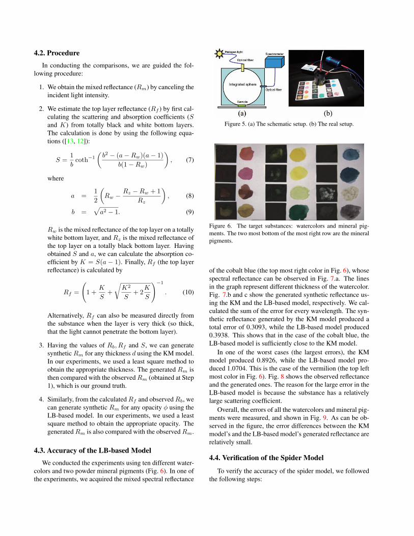
To have accurate measurements, in our experiment weused a spectrometer (Ocean optics’s USB2000+) to acquirespectral data of an object attached to an integrating sphere(LabSphere’s RSA-FO-150) and halogen light (Ocean op-tics’s LS-1), which can provide the incident light intensityand reduce noise from ambient lights. Fig. 5 shows ourexperimental setup. As the target objects, we mainly usedvarious watercolors and powder mineral pigments, wherethe latter were used in wall paintings in Japanese ancienttumuli. Note that, watercolors previously have been shownto follow the KM model [8]. Fig. 6 shows our target sub-stances.
4.2. Procedure
In conducting the comparisons, we are guided the fol-lowing procedure:
1. We obtain the mixed reflectance (Rm) by canceling theincident light intensity.
2. We estimate the top layer reflectance (Rf ) by first cal-culating the scattering and absorption coefficients (Sand K) from totally black and white bottom layers.The calculation is done by using the following equa-tions ([13, 12]):
S =1b
coth−1
(b2 − (a−Rw)(a− 1)
b(1−Rw)
), (7)
where
a =12
(Rw −
Rz −Rw + 1Rz
), (8)
b =√a2 − 1. (9)
Rw is the mixed reflectance of the top layer on a totallywhite bottom layer, and Rz is the mixed reflectance ofthe top layer on a totally black bottom layer. Havingobtained S and a, we can calculate the absorption co-efficient by K = S(a − 1). Finally, Rf (the top layerreflectance) is calculated by
Rf =
(1 +
K
S+
√K2
S+ 2
K
S
)−1
. (10)
Alternatively, Rf can also be measured directly fromthe substance when the layer is very thick (so thick,that the light cannot penetrate the bottom layer).
3. Having the values of Rb, Rf and S, we can generatesyntheticRm for any thickness d using the KM model.In our experiments, we used a least square method toobtain the appropriate thickness. The generated Rm isthen compared with the observedRm (obtained at Step1), which is our ground truth.
4. Similarly, from the calculatedRf and observedRb, wecan generate synthetic Rm for any opacity φ using theLB-based model. In our experiments, we used a leastsquare method to obtain the appropriate opacity. ThegeneratedRm is also compared with the observedRm.
4.3. Accuracy of the LB-based Model
We conducted the experiments using ten different water-colors and two powder mineral pigments (Fig. 6). In one ofthe experiments, we acquired the mixed spectral reflectance
Figure 5. (a) The schematic setup. (b) The real setup.
Figure 6. The target substances: watercolors and mineral pig-ments. The two most bottom of the most right row are the mineralpigments.
of the cobalt blue (the top most right color in Fig. 6), whosespectral reflectance can be observed in Fig. 7.a. The linesin the graph represent different thickness of the watercolor.Fig. 7.b and c show the generated synthetic reflectance us-ing the KM and the LB-based model, respectively. We cal-culated the sum of the error for every wavelength. The syn-thetic reflectance generated by the KM model produced atotal error of 0.3093, while the LB-based model produced0.3938. This shows that in the case of the cobalt blue, theLB-based model is sufficiently close to the KM model.
In one of the worst cases (the largest errors), the KMmodel produced 0.8926, while the LB-based model pro-duced 1.0704. This is the case of the vermilion (the top leftmost color in Fig. 6). Fig. 8 shows the observed reflectanceand the generated ones. The reason for the large error in theLB-based model is because the substance has a relativelylarge scattering coefficient.
Overall, the errors of all the watercolors and mineral pig-ments were measured, and shown in Fig. 9. As can be ob-served in the figure, the error differences between the KMmodel’s and the LB-based model’s generated reflectance arerelatively small.
4.4. Verification of the Spider Model
To verify the accuracy of the spider model, we followedthe following steps:

Figure 7. Experiment target: cobalt blue. Top left: the observedspectra of the substance. The various lines represent the spectra atdifferent locations (thickness). The black dash line is the spectra ofRf . Top right: the generated spectra using the KM model. Bottomleft: the generated spectra using the LB-based model. Bottomright: The values of K/S.
Figure 8. Experiment target: vermilion. Top left: the observedspectra of the substance. The various lines represent the spectra atdifferent locations (thickness). The black dash line is the spectra ofRf . Top right: the generated spectra using the KM model. Bottomleft: the generated spectra using the LB-based model. Bottomright: The values of K/S.
1. Using the procedure described in Section 4.2, we gen-erated the synthetic mixed reflection using the KMmodel and the LB-based model.
2. We chose three values of the spectral reflectance atdifferent wavelengths, representing the peaks of RGBcamera sensitivities (440nm, 552nm, 640nm).
3. We generated many mixed reflectance values bychanging the thickness.
Figure 9. The errors for the simulations of all experiment targets.
Figure 10. The blue lines represent the LB-based model, and thepurple lines represent the KM model. Different lines representdifferent colors.
4. We projected the mixed reflectance values onto a 3Dspace, representing the three wavelengths.
Fig. 10 shows the comparison of the lines in the 3D spacegenerated by the KM model and the LB-based model. Ascan be seen, the generated shapes by the two models are, inmost cases, similar.
Aside from projecting the synthetic reflectance, we alsoverified the distributions of the observed data and the fittingresult of the spider model. We expect that if the fitting resultis sufficiently close for various colors, then the spider modelis reliable in estimating the layered surfaces’ parameters.Fig. 11 shows the fitting of all colorants, which representsthe success of fitting most of the color lines. Note that, inthe figures, there are some location discrepancies betweenthe lines generated by the two models (the yellow and redlines) and the projected points of the pixel intensities (thedark blue points). The reason of this is because, the pixelintensities were acquired by using a digital camera, whilethe lines were calculated from the spectrometer’s data.
5. DiscussionsFrom the experimentation, we can conclude that:
1. We confirm the result of Mudgett et al. [20] that when

Figure 11. The fitting using spider model.The dark blue points are the projection from the input image taken by a digital camera. The bluelines show the results of fitting by the spider model. The yellow lines show the simulation by the LB-based model. The red lines shows thesimulation by the KM model. The yellow and red lines are computed from spectrometer’s data.
scattering is more dominant than absorption, the KMmodel works reliably accurate. This can be observedparticularly in Fig. 8.d. Namely, when K/S is con-siderably small, the synthetic spectra in Fig. 8.b aresimilar to the observed spectra in Fig. 8.a.
2. From Fig. 7 and Fig. 8, in most cases the LB-basedmodel can generate spectra that are similar to those ofthe KM model. However, the result in Fig. 8.d showsthat the LB-based model can be inaccurate when K/Sis considerably small, namely when scattering is moredominant than absorption.
3. Fig. 3.b shows that, in a three-dimensional space(which can be the RGB space), the curves generatedby the KM and the LB-based models are similar. Thisis further shown in Fig. 11, in comparison with the ob-served data.
4. Fig. 11 shows that the spider model can reliably fit tothe observed layered surface data.
5. We confirmed generally the errors of the KM modelare less than LB-based model, as shown in Fig. 9.
6. Overall, importantly the errors of the LB-based model
are relatively small with respect to those of the KMbased model (Fig. 9). Therefore, the LB-based modelis comparable to the KM model, however its model ismuch simpler.
Fig. 12 shows the decomposition result of a few col-orants. The result of the estimated values of F for everypixel is shown in Fig. 12.b, which represents the successof the decomposition using the spider model. However, inFig. 12.b, there are some inaccuracy in the area betweencolor 5 and color 6. This is because their color lines areconsiderably close (implying the inaccuracy was not causedby the spider model).
6. Conclusion
In this paper, we have verified the LB-based model forlayered surfaces from the perspective of the Kubelka-Munk(KM) model, both theoretically and empirically. Besides,we also verified the accuracy of the spider model. We con-sider our verifications can benefit the progress of layered-surface analysis. Since, by being able to show the LB modeland spider model work appropriately for layered surfaces,and to show the conditions where they work, we can haveconsiderable confidence in using the relatively simple mod-els.
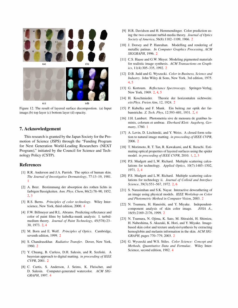
Figure 12. The result of layered surface decompostion. (a) Inputimage.(b) top layer (c) bottom layer (d) opacity.
7. AcknowledgementThis research is granted by the Japan Society for the Pro-
motion of Science (JSPS) through the “Funding Programfor Next Generation World-Leading Researchers (NEXTProgram),” initiated by the Council for Science and Tech-nology Policy (CSTP).
References[1] R.R. Anderson and J.A. Parrish. The optics of human skin.
The Journal of Investigative Dermatology, 77:13–19, 1981.1
[2] A. Beer. Bestimmung der absorption des rothen lichts infarbigen flussigkeiten. Ann. Phys. Chem, 86(2):78–90, 1852.2, 3
[3] R.S. Berns. Principles of color technology. Wiley Inter-science, New York, third edition, 2000. 4
[4] F.W. Billmeyer and R.L. Abrams. Predicting reflectance andcolor of paint films by kubelka-munk analysis: I. turbid-medium theory. Journal of Paint Technology, 45(578):23–30, 1973. 2, 4
[5] M. Born and E. Wolf. Principles of Optics. Cambridge,seventh edition, 1999. 2
[6] S. Chandrasekhar. Radiative Transfer. Dover, New York,1960. 2
[7] Y. Chuang, B. Curless, D.H. Salesin, and R. Szeliski. Abayesian approach to digital matting. in proceeding of IEEECVPR, 2001. 2
[8] C. Curtis, S. Anderson, J. Seims, K. Fleischer, andD. Salesin. Computer-generated watercolor. ACM SIG-GRAPH, 1997. 4
[9] H.R. Davidson and H. Hemmendinger. Color prediction us-ing the two-constant turbid-media theory. Journal of OpticsSociety of America, 56(8):1102–1109, 1966. 2
[10] J. Dorsey and P. Hanrahan. Modelling and rendering ofmetallic patinas. In Computer Graphics Processing, ACMSIGGRAPH, 1996. 2
[11] C.S. Haase and G.W. Meyer. Modeling pigmented materialsfor realistic image synthesis. ACM Transactions on Graph-ics, 11(4):305–335, 1992. 2
[12] D.B. Judd and G. Wyszecki. Color in Business, Science andIndustry. John Wiley & Sons, New York, 3rd edition, 1975.4, 5
[13] G. Kortoum. Reflectance Spectroscopy. Springer-Verlag,New York, 1969. 2, 4, 5
[14] H. Koschmieder. Theorie der horizontalen sichtweite.eitr.Phys. Freien Atm, 12, 1924. 2
[15] P. Kubelka and F. Munk. Ein beitrag zur optik der far-banstriche. Z. Tech. Phys, 12:593–601, 1931. 2, 4
[16] J.H. Lambert. Photometria sive de mensura de gratibus lu-minis, colorum et umbrae. Eberhard Klett: Augsberg, Ger-many, 1760. 1
[17] A. Levin, D. Lischinski, and Y. Weiss. A closed form solu-tion to natural image matting. in proceeding of IEEE CVPR,2006. 2
[18] T. Morimoto, R. T. Tan, R. Kawakami, and K. Ikeuchi. Esti-mating optical properties of layered surfaces using the spidermodel. in proceeding of IEEE CVPR, 2010. 1, 2, 3
[19] P.S. Mudgett and L.W. Richard. Multiple scattering calcu-lations for technology. Applied Optics, 10(7):1485–1502,1971. 2, 4
[20] P.S. Mudgett and L.W. Richard. Multiple scattering calcu-lations for technology ii. Journal of Colloid and InterfaceScience, 39(3):551–567, 1972. 2, 6
[21] S. Narasimhan and S.K. Nayar. Interactive deweathering ofan image using physical models. IEEE Workshop on Colorand Photometric Method in Computer Vision, 2003. 2
[22] N. Tsumura, H. Haneishi, and Y. Miyake. Independent-component analysis of skin color image. JOSA A.,16(9):2169–2176, 1999. 2
[23] N. Tsumura, N. Ojima, K. Sato, M. Shiraishi, H. Shimizu,H. Nabeshima, S. Akazaki, K. Hori, and Y. Miyake. Image-based skin color and texture analysis/synthesis by extractinghemoglobin and melanin information in the skin. ACM SIG-GRAPH, pages 770–779, 2003. 2
[24] G. Wyszecki and W.S. Stiles. Color Science: Concept andMethods, Quantitative Data and Formulae. Wiley Inter-Science, second edition, 1982. 4