accuracy of surface current mapping from high-frequency ... · accuracy of surface current mapping...

55

Accuracy of surface current mapping from High-Frequency (HF) ocean radars

S. CoSoli and G. Bolzon

Istituto Nazionale di Oceanografia e di Geofisica Sperimentale, Trieste, Italy

(Received: March 18, 2014; accepted: August 25, 2014)

ABSTRACT An assessment of surface current mapping accuracy for oceanic High-Frequency (HF) radars is provided. Mapping accuracy is evaluated in terms of radar grid geometry, radial data density and radial velocity errors, and the current field. Mapping errors are derived comparing the original analytical flow pattern with the flow pattern reconstructed varying the error sources. In absence of external perturbations, radar grid geometry controls mapping accuracy and, in combination with asymmetric radial data density, biases both direction and magnitude of surface currents. Flow curvature is an additional source of errors in the surface current maps. Errors are negligible in case of pure zonal or meridional flows with no curvature, but become significant in magnitude and direction when current shears are present. Finally, external perturbations on radial data enhance magnitude and directional biases, thus further degrading vector mapping accuracy.

Key words: HF radar, ocean surface currents, accuracy.

1. Introduction

High-Frequency (HF) ocean radar is a shore-based, remote-sensing technique that provides synoptic views of the sea-state conditions (sea surface current maps; wave parameters) at high temporal (10 min to 1 h) and spatial (500 m to 3 km) resolution. In recent years it spread constantly for academic and research uses, since data are collected over a wide variety of spatial and temporal scales, difficult to achieve with more conventional sampling approaches. HF oceanographic radars are nowadays considered reliable tools in the field of operational oceanography (Paduan et al., 2004), with demonstrated capabilities also as for early-warning systems for tsunami detection (Lipa et al., 2006; Gurgel et al., 2011). HF radars also contribute to improve the skills of ocean circulation models through data assimilation approaches, since their capabilities in resolving rapidly varying current features may help solving processes at a subgrid scale or provide corrections to model wind-forcing (Breivik and Sætra, 2001; Oke et al., 2002; Shulman et al., 2002).

HF radars transmit a radio signal in the 3-30 MHz band and analyze the return signal reflected by ocean surface waves with a wavelength equal to half that of the transmitted signal, to determine the distance, the direction and the velocity of the reflecting surface. This process is known as Bragg scattering (Crombie, 1955), and provides the ocean current velocity in the direction of the transmitter, or radial velocity. The reconstruction of sea-surface vector current map from radial velocity maps is possible when two or more HF radar stations transmit towards the same portion of the ocean, and the signals overlap.

Bollettino di Geofisica Teorica ed Applicata Vol. 56, n. 1, pp. 55-70; March 2015DOI 10.4430/bgta0132

© 2015 – OGS54

Boll. Geof. Teor. Appl., 56, 43-54 Kangazian et al.

Ku C.C. and Sharp J.A.; 1983: Werner deconvolution for automated magnetic interpretation and its refinement using Marquardt inverse modeling. Geophys., 48, 754-774.

Naidu P.S. and Mathew M.P.; 1994: Correlation filtering: a terrain correction method for aeromagnetic maps with application. Appl. Geophys., 32, 269-277.

Rao D.B. and Babu N.R.; 1993: A Fortran-77 computer program for three-dimensional inversion of magnetic anomalies resulting from multiple prismatic bodies. Comput. Geosci., 19, 781-801.

Talwani M.; 1965: Computation with the help of computers of magnetic anomalies caused by bodies of arbitrary shape. Geophys., 30, 797-817.

Tsokas G.N. and Papazachos C.B.; 1992: Two-dimensional inversion filters in magnetic prospecting: application to the exploration for buried antiquities. Geophys., 57, 1004-1013.

Ugalde H. and Morris B.; 2008: An assessment of topographic effects on airborne and ground magnetic data. The Leading Edge, 27, 76-79.

corresponding author: Behrooz Oskooi Dept. of Geomagnetism, Inst. of Geophysics, University of Tehran Kargar shomali, Tehran, Iran Phone: +98 21 88630470, fax: +98 21 88009560, e-mail: [email protected]

56

Boll. Geof. Teor. Appl., 56, 55-70 Cosoli and Bolzon

Error sources in HF radar currents are varied as might be expected for any remotely sensed geophysical signal. Contributions from radiowave interferences, reflections from a moving ship, improper identification of the Bragg peaks, improper determination of the angle of arrival of sea-echo, or wide-area bearing averaging, contribute to errors on radial velocities. Additional errors or uncertainties are introduced during the vector mapping step (Gurgel, 1994) due to variable numbers of available radial currents and to sub-optimal crossing geometry. In the case of uniform radial current uncertainties, the mapping error simplifies to what is referred as the Geometric Dilution Of Precision [GDOP: e.g., Chapman et al. (1997)]. The GDOP is an error multiplier, relating uncertainties in radial and total velocity vectors and describing how radar geometry enhances measurement and position determination errors in radial velocities. Low GDOP values identify an optimal geometric configuration and result in more accurate surface current data. Other sources of errors are random-type errors and as such are expected to become less important as large numbers of observations are used to determine vector velocity maps.

The general reliability of HF radar measurements has been demonstrated through extensive comparisons with a number of independent measurements (current meters, drifters and similar) over a variety of ocean conditions, which provided upper bounds to uncertainties of radial and surface current maps. Typical root-mean-squares (rms) of radar-current meter velocity differences are 7-20 cm/s (Laws et al., 2000, 2010; Emery et al., 2004; Paduan et al., 2006; dePaolo and Terrill, 2007). The relative large rms values derive by both “true” measurement errors from instrumental noise, and the intrinsic geophysical variability related to the different sampling strategies (Chapman and Graber, 1997) or horizontal current shears (Kohut et al., 2012). Validation studies conducted so far have neglected two sources of error: first, the asymmetric distribution of radial velocities from each radar station (the asymmetric radial density distribution effects), though this is considered a major issue in surface current vectors quality control [Level-2 quality control: AA.VV (2005)]; second, the contribution of flow curvature. In the present work, these two error sources are evaluated in relation also to radar grid geometry. The paper is organized as follows. The data and methods, presented in Section 2, describe first the vector mapping process [the least-squares (LS) fit radial-to-vector mapping procedure], and the definition of the flow fields and their decomposition. Section 3 contains the error analysis. Results and conclusions are given in Section 4.

2. Data and methods

2.1. The least-squares mapping approachThe procedure for mapping radial velocities to total currents fits in a LS sense the radial

currents, sampled in a polar coordinate system, onto a regular grid in the area of overlap common to the radar stations (Gurgel, 1994):

(1)

Accuracy of surface current mapping from ocean radars Boll. Geof. Teor. Appl., 56, 55-70

57

In the given equation, qi are the radial angles measured counterclockwise from the positive axis, and the radial velocities. Solution of the system for the eastward and northward components of the surface current vector (U, V) are obtained as:

€

x = A T •A −1( )• A T •b( ) , with, respectively: (2)

(3)

In its original formulation, the LS fit weighted the radial velocities by the variances sR of the ensemble of Doppler velocities that define the radial current (Gurgel, 1994). The common implementations of the algorithm, however, neglect these contributions so that each radial velocity is equally weighted.

Uncertainties in the resulting current vector components depend on uncertainties in radial velocities and on geometrical constraints in the intersecting radar beam geometry (radar’s mean look direction; half-angle between intersecting beams), and are commonly quantified in terms of the GDOP (Gurgel, 1994; Chapman et al., 1997; Chavanne et al., 2007). However, it should be pointed out that it is not sufficient to give uncertainties for the zonal and meridional components of current vectors, as they cannot be estimated independently from each other, and are therefore correlated (Chavanne et al., 2007).

Ideally, the total current vector is unambiguously resolved for orthogonal or nearly orthogonal intersecting beams. In practice, orthogonality constraints are relaxed and a wider range of angles defining an “optimal intersection” region is accepted, that typically span the range 30˚≤θ≤150˚ (Shay et al., 2007). Clearly, mapping biases increase as departures from the orthogonality constraint increase, and thus physical significance of the measurements in these areas should be carefully assessed. In the implementation of the LS procedure, the fit is applied to radials falling within a radius R around an arbitrary grid location. The distance R is usually set in such a manner to include as many radials as possible in the vector mapping process, so to improve the statistical robustness of the current vector estimate while preserving as much as possible the surrounding grid points from spurious numerical correlation.

2.2. Definition of the analytical flow fields and error metricsThe error analysis consists in the determination of mapping errors or magnitude - direction

biases between prescribed and reconstructed flow patterns in relation to the chosen error source. The prescribed flow patterns are first converted to polar-coordinates radial maps, that is, they are decomposed as if “seen” by two distinct radars by projecting the velocity vectors at each grid point in the direction of each radar site. Then, they are mapped back on the vector grid -without additional or with additional external perturbations as described in Eqs. (2) and (3), and compared to the original flow structures to determine magnitude and directional biases. Mapping is performed using both unperturbed and perturbed radials; perturbations are introduced as randomly distributed noise with prescribed standard deviation, and randomly distributed gaps in radial coverage, so to simulate radial current errors and more closely match

56


Error sources in HF radar currents are varied as might be expected for any remotely sensed geophysical signal. Contributions from radiowave interferences, reflections from a moving ship, improper identification of the Bragg peaks, improper determination of the angle of arrival of sea-echo, or wide-area bearing averaging, contribute to errors on radial velocities. Additional errors or uncertainties are introduced during the vector mapping step (Gurgel, 1994) due to variable numbers of available radial currents and to sub-optimal crossing geometry. In the case of uniform radial current uncertainties, the mapping error simplifies to what is referred as the Geometric Dilution Of Precision [GDOP: e.g., Chapman et al. (1997)]. The GDOP is an error multiplier, relating uncertainties in radial and total velocity vectors and describing how radar geometry enhances measurement and position determination errors in radial velocities. Low GDOP values identify an optimal geometric configuration and result in more accurate surface current data. Other sources of errors are random-type errors and as such are expected to become less important as large numbers of observations are used to determine vector velocity maps.

The general reliability of HF radar measurements has been demonstrated through extensive comparisons with a number of independent measurements (current meters, drifters and similar) over a variety of ocean conditions, which provided upper bounds to uncertainties of radial and surface current maps. Typical root-mean-squares (rms) of radar-current meter velocity differences are 7-20 cm/s (Laws et al., 2000, 2010; Emery et al., 2004; Paduan et al., 2006; dePaolo and Terrill, 2007). The relative large rms values derive by both “true” measurement errors from instrumental noise, and the intrinsic geophysical variability related to the different sampling strategies (Chapman and Graber, 1997) or horizontal current shears (Kohut et al., 2012). Validation studies conducted so far have neglected two sources of error: first, the asymmetric distribution of radial velocities from each radar station (the asymmetric radial density distribution effects), though this is considered a major issue in surface current vectors quality control [Level-2 quality control: AA.VV (2005)]; second, the contribution of flow curvature. In the present work, these two error sources are evaluated in relation also to radar grid geometry. The paper is organized as follows. The data and methods, presented in Section 2, describe first the vector mapping process [the least-squares (LS) fit radial-to-vector mapping procedure], and the definition of the flow fields and their decomposition. Section 3 contains the error analysis. Results and conclusions are given in Section 4.

2. Data and methods

2.1. The least-squares mapping approachThe procedure for mapping radial velocities to total currents fits in a LS sense the radial

currents, sampled in a polar coordinate system, onto a regular grid in the area of overlap common to the radar stations (Gurgel, 1994):

(1)

58


experimental conditions. To simulate the effects of asymmetric radial data distributions, vectors are reconstructed allowing radial data density from the two sites (ni, with i = 1, 2 the site indexes) to vary in the range (nmin = 1; nmax = 30).

The simplified radar network mimics the typical set-up of an experimental network of ocean radars working in the 25 MHz frequency band, and consist of two HF radars 20 km apart, having 1.5 km resolution in range and 5˚ resolution in angle.

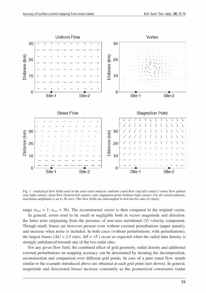
The chosen analytical flow patterns are defined on a regular grid with 1x1 km spatial resolution, and include (Fig. 1): a uniform zonal current pattern (30 cm/s magnitude); a vortex, with tangential velocities

Vθ = v(R, θ), ,

and Vmax = 30 cm/s-1 at Rmax = 10 km from the centre of the vortex; a shear flow: and Umax = 30 cm/s-1; and, a stagnation point: U = cx; V = – cy.

The comparison metrics that quantifies the mapping error and, conversely, gives the mapping accuracy, determines the biases on vector components

,

on flow direction , and relative

error between the components of the synthetic (original) and the reconstructed current vectors, (Us, Vs) and (Ur, Vr).

3. Error analysis

3.1. Radial density, grid geometry and vector accuracyThe first point to investigate is the relation between mapping accuracy and radial

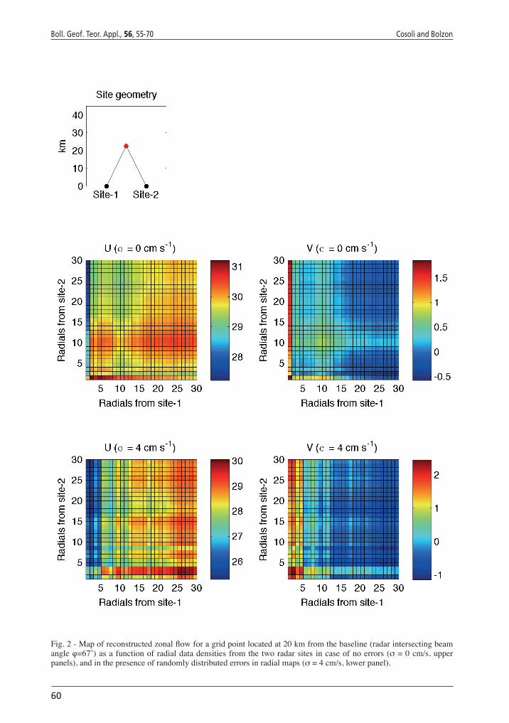
data density distribution, and in particular, the influence of symmetric-asymmetric radial distributions on mapping accuracy. Ideally, accuracy increases when a large amount of radials is used and when radial contribution is equally distributed between contributing sites. This is due to the fact that most of the error sources to HF radar-derived radial currents are random and become less important as large numbers of observations are merged. A symmetrical radial density distribution, in turn, has the advantage of equally weighting each measuring station, reducing thus any bias. In practice, hardware or software failures often limit data availability with a consequent degradation of the mapping accuracy; or, grid geometry and angular resolution favor one site more than the second one.The influence of asymmetrical radial velocity distribution on mapping accuracy can be assessed as follows. For simplicity the analysis is performed on a 30 cm/s zonal (E-W) vector (Fig. 2). After being decomposed in radial components for the two radar stations, the radial components are replicated N times, and the vector is reconstructed as described in Section 2.a using different amounts of radial velocities from the two sites (ni, i = 1, 2 staying for the site indexes) in the


59

range (nmin = 1; nmax = 30). The reconstructed vector is then compared to the original vector.In general, errors tend to be small or negligible both in vector magnitude and direction,

the latter term originating from the presence of non-zero meridional (V) velocity component. Though small, biases are however present even without external perturbations (upper panels), and increase when noise is included. In both cases (without perturbations; with perturbations), the largest biases (ΔU = 2.5 cm/s; Δθ = 15˚) occur as expected when the radial data density is strongly unbalanced towards any of the two radar sites.

For any given flow field, the combined effect of grid geometry, radial density and additional external perturbations on mapping accuracy can be determined by iterating the decomposition, reconstruction and comparison over different grid points. In case of a pure zonal flow, trends similar to the example introduced above are obtained at each grid point (not shown). In general, magnitude and directional biases increase constantly as the geometrical constraints (radar

Fig. 1 - Analytical flow fields used in the error error analysis: uniform zonal flow (top left corner); vortex flow pattern (top right corner); shear flow (bottom left corner); and, stagnation point (bottom right corner). For all current patterns, maximum amplitude is set to 30 cm/s. The flow fields are subsampled to 4x4 km for sake of clarity.

58


experimental conditions. To simulate the effects of asymmetric radial data distributions, vectors are reconstructed allowing radial data density from the two sites (ni, with i = 1, 2 the site indexes) to vary in the range (nmin = 1; nmax = 30).

The simplified radar network mimics the typical set-up of an experimental network of ocean radars working in the 25 MHz frequency band, and consist of two HF radars 20 km apart, having 1.5 km resolution in range and 5˚ resolution in angle.

The chosen analytical flow patterns are defined on a regular grid with 1x1 km spatial resolution, and include (Fig. 1): a uniform zonal current pattern (30 cm/s magnitude); a vortex, with tangential velocities

Vθ = v(R, θ), ,

and Vmax = 30 cm/s-1 at Rmax = 10 km from the centre of the vortex; a shear flow: and Umax = 30 cm/s-1; and, a stagnation point: U = cx; V = – cy.

The comparison metrics that quantifies the mapping error and, conversely, gives the mapping accuracy, determines the biases on vector components

,

on flow direction , and relative

error between the components of the synthetic (original) and the reconstructed current vectors, (Us, Vs) and (Ur, Vr).

3. Error analysis

3.1. Radial density, grid geometry and vector accuracyThe first point to investigate is the relation between mapping accuracy and radial

data density distribution, and in particular, the influence of symmetric-asymmetric radial distributions on mapping accuracy. Ideally, accuracy increases when a large amount of radials is used and when radial contribution is equally distributed between contributing sites. This is due to the fact that most of the error sources to HF radar-derived radial currents are random and become less important as large numbers of observations are merged. A symmetrical radial density distribution, in turn, has the advantage of equally weighting each measuring station, reducing thus any bias. In practice, hardware or software failures often limit data availability with a consequent degradation of the mapping accuracy; or, grid geometry and angular resolution favor one site more than the second one.The influence of asymmetrical radial velocity distribution on mapping accuracy can be assessed as follows. For simplicity the analysis is performed on a 30 cm/s zonal (E-W) vector (Fig. 2). After being decomposed in radial components for the two radar stations, the radial components are replicated N times, and the vector is reconstructed as described in Section 2.a using different amounts of radial velocities from the two sites (ni, i = 1, 2 staying for the site indexes) in the

60


Fig. 2 - Map of reconstructed zonal flow for a grid point located at 20 km from the baseline (radar intersecting beam angle φ=67˚) as a function of radial data densities from the two radar sites in case of no errors (s = 0 cm/s, upper panels), and in the presence of randomly distributed errors in radial maps (s = 4 cm/s, lower panel).


61

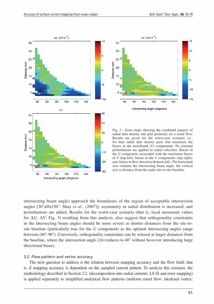
intersecting beam angle) approach the boundaries of the region of acceptable intersection angles [30˚≤θ≤150˚: Shay et al., (2007)], asymmetry in radial distribution is increased, and perturbations are added. Results for the worst-case scenario (that is, local maximum values for ΔU, ΔV: Fig. 3) resulting from this analysis, also suggest that orthogonality constraints in the intersecting beam angles should be more severe at shorter distances from the site-to-site baseline (particularly true for the U component) as the optimal intersecting angles range between (60˚-90˚). Conversely, orthogonality constraints can be relaxed at larger distances from the baseline, where the intersection angle (2Ø) reduces to 40˚ without however introducing large directional biases.

3.2. Flow pattern and vector accuracyThe next question to address is the relation between mapping accuracy and the flow field; that

is, if mapping accuracy is dependent on the sampled current pattern. To analyze this scenario, the methodology described in Section 2.2. (decomposition into radial currents, LS fit and error mapping) is applied separately to simplified analytical flow patterns (uniform zonal flow; idealized vortex;

Fig. 3 - Error maps showing the combined impacts of radial data density and grid geometry on a zonal flow. Results are given for the worst-case scenario, i.e., for data radial data density pairs that maximize the biases in the meridional (V) components. No external perturbations are applied to radial velocities. Biases in the U component, associated with the maximum biases in V (top left); biases in the V components (top right); and, biases in flow direction (bottom left). The horizontal axis contains the intersecting beam angle, the vertical axis is distance from the radar site-to-site baseline.

60


Fig. 2 - Map of reconstructed zonal flow for a grid point located at 20 km from the baseline (radar intersecting beam angle φ=67˚) as a function of radial data densities from the two radar sites in case of no errors (s = 0 cm/s, upper panels), and in the presence of randomly distributed errors in radial maps (s = 4 cm/s, lower panel).

62


shear-flow; stagnation point: Fig. 1), and effects of perturbations are evaluated by introducing errors on radial current maps and additional randomly-distributed gaps in radial coverage.

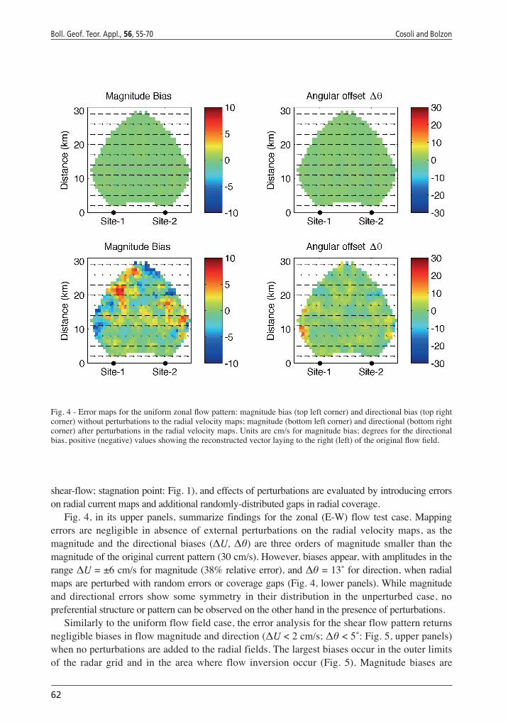
Fig. 4, in its upper panels, summarize findings for the zonal (E-W) flow test case. Mapping errors are negligible in absence of external perturbations on the radial velocity maps, as the magnitude and the directional biases (ΔU, Δθ) are three orders of magnitude smaller than the magnitude of the original current pattern (30 cm/s). However, biases appear, with amplitudes in the range ΔU = ±6 cm/s for magnitude (38% relative error), and Δθ = 13˚ for direction, when radial maps are perturbed with random errors or coverage gaps (Fig. 4, lower panels). While magnitude and directional errors show some symmetry in their distribution in the unperturbed case, no preferential structure or pattern can be observed on the other hand in the presence of perturbations.

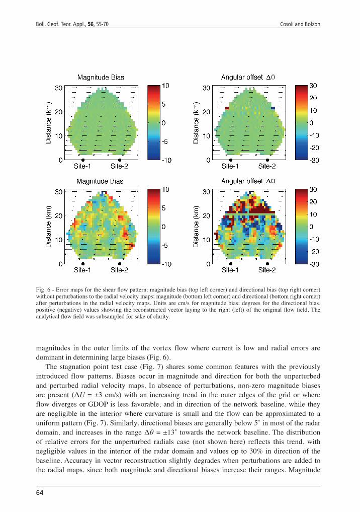
Similarly to the uniform flow field case, the error analysis for the shear flow pattern returns negligible biases in flow magnitude and direction (ΔU < 2 cm/s; Δθ < 5˚: Fig. 5, upper panels) when no perturbations are added to the radial fields. The largest biases occur in the outer limits of the radar grid and in the area where flow inversion occur (Fig. 5). Magnitude biases are

Fig. 4 - Error maps for the uniform zonal flow pattern: magnitude bias (top left corner) and directional bias (top right corner) without perturbations to the radial velocity maps; magnitude (bottom left corner) and directional (bottom right corner) after perturbations in the radial velocity maps. Units are cm/s for magnitude bias; degrees for the directional bias, positive (negative) values showing the reconstructed vector laying to the right (left) of the original flow field.


63

larger in the perturbed radial case for both magnitude and direction. However, with respect to the unperturbed radials, magnitude biases are almost uniformly distributed within the radar area, whereas directional biases show a preferential clustering in proximity of the flow inversion.

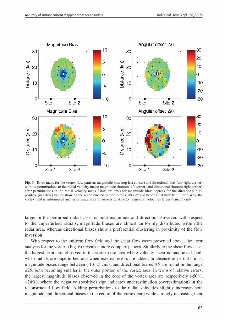
With respect to the uniform flow field and the shear flow cases presented above, the error analysis for the vortex (Fig. 6) reveals a more complex pattern. Similarly to the shear flow case, the largest errors are observed in the vortex core area where velocity shear is maximized, both when radials are unperturbed and when external errors are added. In absence of perturbations, magnitude biases range between (-13, 2) cm/s, and directional biases Δθ are found in the range ±25, both becoming smaller in the outer portion of the vortex area. In terms of relative errors, the largest magnitude biases observed in the core of the vortex area are respectively (-50%, +24%), where the negative (positive) sign indicates underestimation (overestimation) in the reconstructed flow field. Adding perturbations to the radial velocities slightly increases both magnitude and directional biases in the centre of the vortex core while strongly increasing their

Fig. 5 - Error maps for the vortex flow pattern: magnitude bias (top left corner) and directional bias (top right corner) without perturbations to the radial velocity maps; magnitude (bottom left corner) and directional (bottom right corner) after perturbations in the radial velocity maps. Units are cm/s for magnitude bias; degrees for the directional bias, positive (negative) values showing the reconstructed vector to the right (left) of the original flow field. For clarity, the vortex field is subsampled and error maps are shown only relative to tangential velocities larger than 2.5 cm/s.

62


shear-flow; stagnation point: Fig. 1), and effects of perturbations are evaluated by introducing errors on radial current maps and additional randomly-distributed gaps in radial coverage.

Fig. 4, in its upper panels, summarize findings for the zonal (E-W) flow test case. Mapping errors are negligible in absence of external perturbations on the radial velocity maps, as the magnitude and the directional biases (ΔU, Δθ) are three orders of magnitude smaller than the magnitude of the original current pattern (30 cm/s). However, biases appear, with amplitudes in the range ΔU = ±6 cm/s for magnitude (38% relative error), and Δθ = 13˚ for direction, when radial maps are perturbed with random errors or coverage gaps (Fig. 4, lower panels). While magnitude and directional errors show some symmetry in their distribution in the unperturbed case, no preferential structure or pattern can be observed on the other hand in the presence of perturbations.

Similarly to the uniform flow field case, the error analysis for the shear flow pattern returns negligible biases in flow magnitude and direction (ΔU < 2 cm/s; Δθ < 5˚: Fig. 5, upper panels) when no perturbations are added to the radial fields. The largest biases occur in the outer limits of the radar grid and in the area where flow inversion occur (Fig. 5). Magnitude biases are

Fig. 4 - Error maps for the uniform zonal flow pattern: magnitude bias (top left corner) and directional bias (top right corner) without perturbations to the radial velocity maps; magnitude (bottom left corner) and directional (bottom right corner) after perturbations in the radial velocity maps. Units are cm/s for magnitude bias; degrees for the directional bias, positive (negative) values showing the reconstructed vector laying to the right (left) of the original flow field.

64


magnitudes in the outer limits of the vortex flow where current is low and radial errors are dominant in determining large biases (Fig. 6).

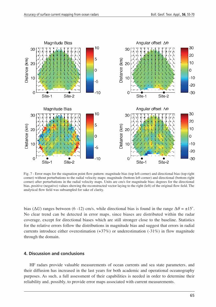
The stagnation point test case (Fig. 7) shares some common features with the previously introduced flow patterns. Biases occur in magnitude and direction for both the unperturbed and perturbed radial velocity maps. In absence of perturbations, non-zero magnitude biases are present (ΔU = ±3 cm/s) with an increasing trend in the outer edges of the grid or where flow diverges or GDOP is less favorable, and in direction of the network baseline, while they are negligible in the interior where curvature is small and the flow can be approximated to a uniform pattern (Fig. 7). Similarly, directional biases are generally below 5˚ in most of the radar domain, and increases in the range Δθ = ±13˚ towards the network baseline. The distribution of relative errors for the unperturbed radials case (not shown here) reflects this trend, with negligible values in the interior of the radar domain and values op to 30% in direction of the baseline. Accuracy in vector reconstruction slightly degrades when perturbations are added to the radial maps, since both magnitude and directional biases increase their ranges. Magnitude

Fig. 6 - Error maps for the shear flow pattern: magnitude bias (top left corner) and directional bias (top right corner) without perturbations to the radial velocity maps; magnitude (bottom left corner) and directional (bottom right corner) after perturbations in the radial velocity maps. Units are cm/s for magnitude bias; degrees for the directional bias, positive (negative) values showing the reconstructed vector laying to the right (left) of the original flow field. The analytical flow field was subsampled for sake of clarity.


65

bias (ΔU) ranges between (6 -12) cm/s, while directional bias is found in the range Δθ = ±15˚. No clear trend can be detected in error maps, since biases are distributed within the radar coverage, except for directional biases which are still stronger close to the baseline. Statistics for the relative errors follow the distributions in magnitude bias and suggest that errors in radial currents introduce either overestimation (+37%) or underestimation (-31%) in flow magnitude through the domain.

4. Discussion and conclusions

HF radars provide valuable measurements of ocean currents and sea state parameters, and their diffusion has increased in the last years for both academic and operational oceanography purposes. As such, a full assessment of their capabilities is needed in order to determine their reliability and, possibly, to provide error maps associated with current measurements.

Fig. 7 - Error maps for the stagnation point flow pattern: magnitude bias (top left corner) and directional bias (top right corner) without perturbations to the radial velocity maps; magnitude (bottom left corner) and directional (bottom right corner) after perturbations in the radial velocity maps. Units are cm/s for magnitude bias; degrees for the directional bias, positive (negative) values showing the reconstructed vector laying to the right (left) of the original flow field. The analytical flow field was subsampled for sake of clarity.

64


magnitudes in the outer limits of the vortex flow where current is low and radial errors are dominant in determining large biases (Fig. 6).

The stagnation point test case (Fig. 7) shares some common features with the previously introduced flow patterns. Biases occur in magnitude and direction for both the unperturbed and perturbed radial velocity maps. In absence of perturbations, non-zero magnitude biases are present (ΔU = ±3 cm/s) with an increasing trend in the outer edges of the grid or where flow diverges or GDOP is less favorable, and in direction of the network baseline, while they are negligible in the interior where curvature is small and the flow can be approximated to a uniform pattern (Fig. 7). Similarly, directional biases are generally below 5˚ in most of the radar domain, and increases in the range Δθ = ±13˚ towards the network baseline. The distribution of relative errors for the unperturbed radials case (not shown here) reflects this trend, with negligible values in the interior of the radar domain and values op to 30% in direction of the baseline. Accuracy in vector reconstruction slightly degrades when perturbations are added to the radial maps, since both magnitude and directional biases increase their ranges. Magnitude

Fig. 6 - Error maps for the shear flow pattern: magnitude bias (top left corner) and directional bias (top right corner) without perturbations to the radial velocity maps; magnitude (bottom left corner) and directional (bottom right corner) after perturbations in the radial velocity maps. Units are cm/s for magnitude bias; degrees for the directional bias, positive (negative) values showing the reconstructed vector laying to the right (left) of the original flow field. The analytical flow field was subsampled for sake of clarity.

66


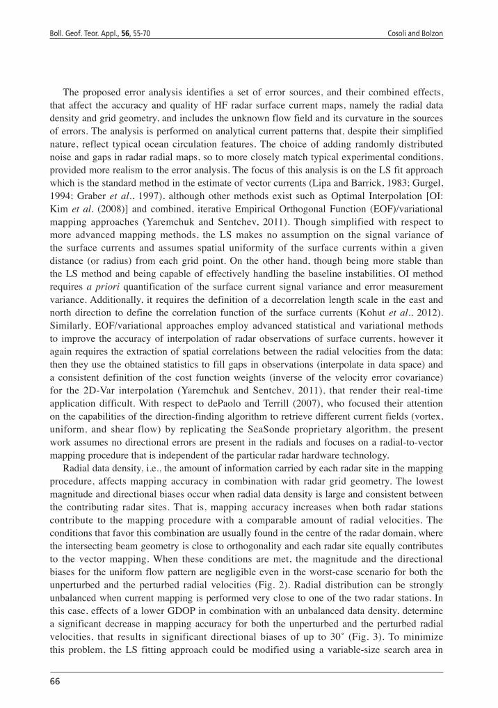
The proposed error analysis identifies a set of error sources, and their combined effects, that affect the accuracy and quality of HF radar surface current maps, namely the radial data density and grid geometry, and includes the unknown flow field and its curvature in the sources of errors. The analysis is performed on analytical current patterns that, despite their simplified nature, reflect typical ocean circulation features. The choice of adding randomly distributed noise and gaps in radar radial maps, so to more closely match typical experimental conditions, provided more realism to the error analysis. The focus of this analysis is on the LS fit approach which is the standard method in the estimate of vector currents (Lipa and Barrick, 1983; Gurgel, 1994; Graber et al., 1997), although other methods exist such as Optimal Interpolation [OI: Kim et al. (2008)] and combined, iterative Empirical Orthogonal Function (EOF)/variational mapping approaches (Yaremchuk and Sentchev, 2011). Though simplified with respect to more advanced mapping methods, the LS makes no assumption on the signal variance of the surface currents and assumes spatial uniformity of the surface currents within a given distance (or radius) from each grid point. On the other hand, though being more stable than the LS method and being capable of effectively handling the baseline instabilities, OI method requires a priori quantification of the surface current signal variance and error measurement variance. Additionally, it requires the definition of a decorrelation length scale in the east and north direction to define the correlation function of the surface currents (Kohut et al., 2012). Similarly, EOF/variational approaches employ advanced statistical and variational methods to improve the accuracy of interpolation of radar observations of surface currents, however it again requires the extraction of spatial correlations between the radial velocities from the data; then they use the obtained statistics to fill gaps in observations (interpolate in data space) and a consistent definition of the cost function weights (inverse of the velocity error covariance) for the 2D-Var interpolation (Yaremchuk and Sentchev, 2011), that render their real-time application difficult. With respect to dePaolo and Terrill (2007), who focused their attention on the capabilities of the direction-finding algorithm to retrieve different current fields (vortex, uniform, and shear flow) by replicating the SeaSonde proprietary algorithm, the present work assumes no directional errors are present in the radials and focuses on a radial-to-vector mapping procedure that is independent of the particular radar hardware technology.

Radial data density, i.e., the amount of information carried by each radar site in the mapping procedure, affects mapping accuracy in combination with radar grid geometry. The lowest magnitude and directional biases occur when radial data density is large and consistent between the contributing radar sites. That is, mapping accuracy increases when both radar stations contribute to the mapping procedure with a comparable amount of radial velocities. The conditions that favor this combination are usually found in the centre of the radar domain, where the intersecting beam geometry is close to orthogonality and each radar site equally contributes to the vector mapping. When these conditions are met, the magnitude and the directional biases for the uniform flow pattern are negligible even in the worst-case scenario for both the unperturbed and the perturbed radial velocities (Fig. 2). Radial distribution can be strongly unbalanced when current mapping is performed very close to one of the two radar stations. In this case, effects of a lower GDOP in combination with an unbalanced data density, determine a significant decrease in mapping accuracy for both the unperturbed and the perturbed radial velocities, that results in significant directional biases of up to 30˚ (Fig. 3). To minimize this problem, the LS fitting approach could be modified using a variable-size search area in


67

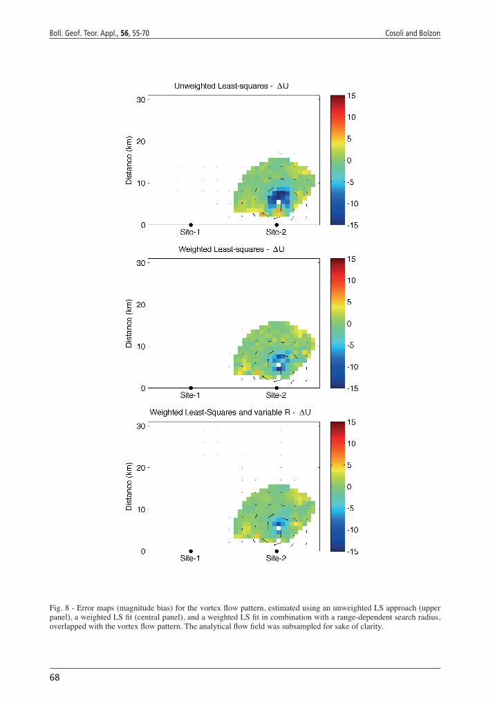
combination with an appropriate weighting function to be applied on the radial velocities (such, for instance, a weight inversely proportional to the distance from the grid point), so to balance radial data density while providing at the same time the proper weight to radial velocities closer to the radar grid point, as suggested for a vortex flow (Fig. 8).

Results of the error analysis on synthetic flow patterns suggest the presence of systematic bias in the LS fit mapping approach that is somehow dependent on the flow pattern and its curvature. The vector mapping approach, in fact, generally succeeds in retrieving the spatial pattern of the current field both in absence and in presence of errors. However, it may introduce a systematic underestimation in current speed magnitude, which is negligible in case of the uniform flow field (errors below 10-3 cm/s for a pure zonal flow pattern with 30 cm/s magnitude and no perturbation to radial velocities). Biases as large as 31% (overestimation error) are found for the stagnation point pattern, as large as 50% (underestimation error) for the vortex flow, and as large as 83% (underestimation error) for the shear flow. Any additional error on the radial maps enhances the mapping errors for all the flow patterns, regardless of the current shear in the flow.

In general, the curvature-related error term is maximized in the area of maximum current shear, for instance in the centre of the vortex or in the area where the shear flow pattern presents flow reversal and to some extent is proportional to the slope parameter (c) that defines the curvature in the analytical flow patterns, as tests performed on the shear flow suggested (not shown here). This result suggests thus some proportionality between the radial velocity gradient

Ur and the distance Dr where radial velocities are sampled, and error mapping (ΔU) in the form . The present analysis shows that mapping accuracy depend also on radial data density, and that mapping accuracy increases with the amount of radial information from each radar station, and also on the ocean current pattern and its shear. As pointed out in Kohut et al. (2012), weighting radial currents with an appropriate weighting function could reduce the effects of current shear and improve radial-to-vector mapping accuracy. One way to optimize radial data density contribution is to increase the size of the search area with distance from each site, in combination with a proper weighting function that preserves as much as possible surrounding grid points from spurious numerical correlations. This option is currently being developed and tested on the same analytical flow pattern used in the present analysis. Preliminary results of the weighted LS fit with variable search radius using an exponential curve for the weight function and a linearly increasing distance in the range (Rmin = 1 km; Rmax = 3 km) for the search radius, show a decrease in directional and magnitude biases with a general improvement in overall mapping accuracy for all the considered analytical flow fields. An example is given in Fig. 8, which compares the unweighted LS (upper panel) with the weighted LS (middle panel) and the weighted LS combined with a variable search radius for a vortex field, displaced in proximity of the second radar station.

The definition of the optimal parameters for the weighting function and the search radius requires further fine-tuning analyses and assessment over a wider set of current patterns so to match more closely ocean currents variability on a regional scale. Despite its simplified approach the present assessment analysis provides a useful analysis to quantify mapping errors and uncertainties in remotely-sensed current maps.

66


The proposed error analysis identifies a set of error sources, and their combined effects, that affect the accuracy and quality of HF radar surface current maps, namely the radial data density and grid geometry, and includes the unknown flow field and its curvature in the sources of errors. The analysis is performed on analytical current patterns that, despite their simplified nature, reflect typical ocean circulation features. The choice of adding randomly distributed noise and gaps in radar radial maps, so to more closely match typical experimental conditions, provided more realism to the error analysis. The focus of this analysis is on the LS fit approach which is the standard method in the estimate of vector currents (Lipa and Barrick, 1983; Gurgel, 1994; Graber et al., 1997), although other methods exist such as Optimal Interpolation [OI: Kim et al. (2008)] and combined, iterative Empirical Orthogonal Function (EOF)/variational mapping approaches (Yaremchuk and Sentchev, 2011). Though simplified with respect to more advanced mapping methods, the LS makes no assumption on the signal variance of the surface currents and assumes spatial uniformity of the surface currents within a given distance (or radius) from each grid point. On the other hand, though being more stable than the LS method and being capable of effectively handling the baseline instabilities, OI method requires a priori quantification of the surface current signal variance and error measurement variance. Additionally, it requires the definition of a decorrelation length scale in the east and north direction to define the correlation function of the surface currents (Kohut et al., 2012). Similarly, EOF/variational approaches employ advanced statistical and variational methods to improve the accuracy of interpolation of radar observations of surface currents, however it again requires the extraction of spatial correlations between the radial velocities from the data; then they use the obtained statistics to fill gaps in observations (interpolate in data space) and a consistent definition of the cost function weights (inverse of the velocity error covariance) for the 2D-Var interpolation (Yaremchuk and Sentchev, 2011), that render their real-time application difficult. With respect to dePaolo and Terrill (2007), who focused their attention on the capabilities of the direction-finding algorithm to retrieve different current fields (vortex, uniform, and shear flow) by replicating the SeaSonde proprietary algorithm, the present work assumes no directional errors are present in the radials and focuses on a radial-to-vector mapping procedure that is independent of the particular radar hardware technology.

Radial data density, i.e., the amount of information carried by each radar site in the mapping procedure, affects mapping accuracy in combination with radar grid geometry. The lowest magnitude and directional biases occur when radial data density is large and consistent between the contributing radar sites. That is, mapping accuracy increases when both radar stations contribute to the mapping procedure with a comparable amount of radial velocities. The conditions that favor this combination are usually found in the centre of the radar domain, where the intersecting beam geometry is close to orthogonality and each radar site equally contributes to the vector mapping. When these conditions are met, the magnitude and the directional biases for the uniform flow pattern are negligible even in the worst-case scenario for both the unperturbed and the perturbed radial velocities (Fig. 2). Radial distribution can be strongly unbalanced when current mapping is performed very close to one of the two radar stations. In this case, effects of a lower GDOP in combination with an unbalanced data density, determine a significant decrease in mapping accuracy for both the unperturbed and the perturbed radial velocities, that results in significant directional biases of up to 30˚ (Fig. 3). To minimize this problem, the LS fitting approach could be modified using a variable-size search area in

68


Fig. 8 - Error maps (magnitude bias) for the vortex flow pattern, estimated using an unweighted LS approach (upper panel), a weighted LS fit (central panel), and a weighted LS fit in combination with a range-dependent search radius, overlapped with the vortex flow pattern. The analytical flow field was subsampled for sake of clarity.


69

RefeRenceS

AA.VV.; 2005: In: Second workshop report on the quality assurance of real-time ocean data, CCPO, Norfolk, VA, USA, Technical Report Series 05-01, 48 pp.

Breivik O. and Sætra O.; 2001: Real time assimilation of radar currents into a coastal ocean model. J. Mar. Syst., 28, 161-182.

Chapman R.D. and Graber H.C.; 1997: Validation of HF radar measurements. Oceanogr., 10, 76-79.

Chapman R.D., Shay L.K., Graber H.C., Edson J.B., Karachintsev A., Trump C.L. and Ross D.B.; 1997: On the accuracy of HF radar surface current measurements: intercomparisons with ship-based sensors. J. Geophys. Res, 102, 18737-18748.

Chavanne C., Janekovic I., Flament P., Poulain P.-M., Kuzmic M. and Gurgel K.-W.; 2007: Tidal currents in the northwestern Adriatic: high-frequency radar observations and numerical model predictions. J. Geophys. Res., 112, C03S21, doi:10.1029/2006JC003523.

Crombie D.D.; 1955: Doppler spectrum of sea echo at 13.56 Mc/s. Nature, 175, 681-682.

dePaolo T. and Terrill E.; 2007: Skill assessment of resolving ocean surface current structure using compact-antenna style HF radar and MUSIC direction finding algorithm. J. Atmos. Oceanic Technol., 24, 1277-1300.

Emery B.M., Washburn L. and Harlan J.A.; 2004: Evaluating radial current measurements from CODAR high-frequency radars with moored current meters. J. Atmos. Oceanic Technol., 21, 1259-1271.

Graber H.C., Haus B.K., Chapman R.D. and Shay L.K.; 1997: HF radar comparisons with moored estimates of current speed and direction: expected differences and implications. J. Geophys. Res., 102, 18749–18766.

Gurgel K.W.; 1994: Shipborne measurement of surface current fields by HF radar. L’Onde Electr., 74, 54-59.

Gurgel K.W., Dzvonkovskaya A., Pohlmann T., Schlick T. and Gill E.; 2011: Simulation and detection of tsunami features in ocean surface currents measured by HF radars. Ocean Dyn., 10, 1495-1507, doi: 10.1007/s10236-011-0420-9.

Kim S.Y. Terrill E.J. and Cornuelle B.D.; 2008: Mapping surface currents from HF radar radial velocity measurements using optimal interpolation. J. Geophys. Res., 113, C10023, doi: 10.1029/2007JC004244.

Kohut J., Roarty H., Randall-Goodwin E., Glenn S. and Lichtenwalner C.S.; 2012: Evaluation of two algorithms for a nework of coastal HF radars in the Mid-Atlantic Bight. Ocean Dyn., 62, 953-968, doi: 10.1007/s10236-012-0533-9.

Laws K.E., Fernandez D.M. and Paduan J.D.; 2000: Simulation-based evaluations of HF radar ocean current algorithms. IEEE J. Oceanic Eng., 25, 481-491.

Laws K.E., Paduan J.D. and Vesecky J.; 2010: Estimation and assessment of errors related to antenna pattern distortion in CODAR SeaSonde High-Frequency radar ocean current measurements. J. Atmos. Oceanic Technol., 27, 1029-1043, doi: 10.1175/2009JTECHO658.1.

Lipa B.J. and Barrick D.E.; 1983: Least-squares methods for the extraction of surface currents from CODAR crossed-loop data: application at ARSLOE. IEEE J. Oceanic Eng., 13, 507-513.

Lipa B.J., Barrick D.E., Bourg J. and Nyden B.B; 2006: HF radar detection of tsunamis. J. Oceanogr., 62, 705-716.

Oke P., Allen J.S., Miller R.N., Egbert G.D. and Kosro P.M.; 2002: Assimilation of surface velocity data into a primitive equation coastal ocean model. J. Geophys. Res., 107, 3122, doi: 10.1029/2000JC000511.

Paduan J.D., Kosro P.M. and Glenn S.M.; 2004: A national coastal ocean surface current mapping system for the United States. Mar. Tech. Soc. J., 38, 102-108.

Paduan J.D., Kim K.C., Cook M.S. and Chavez F.P.; 2006: Calibration and validation of direction-finding high-frequency radar ocean surface current observations. IEEE J. Oceanic Eng., 31, doi: 10.1109/JOE.2006.886195.

Shay L.K., Martinez-Pedraja J., Cook T.M. and Haus B.K.; 2007: High frequency surface current mapping using Wellen Radar. J. Atmos. Oceanic Technol., 24, 484-503, doi: 10.1175/JTECH1985.1

68


Fig. 8 - Error maps (magnitude bias) for the vortex flow pattern, estimated using an unweighted LS approach (upper panel), a weighted LS fit (central panel), and a weighted LS fit in combination with a range-dependent search radius, overlapped with the vortex flow pattern. The analytical flow field was subsampled for sake of clarity.

70


Shulman I., Wu C.R., Lewis J.K., Paduan J.D., Rosenfeld L.K., Kindle J.C., Ramp S.R. and Collins C.A.; 2002: High resolution modeling and data assimilation in the Monterey Bay area. Cont. Shelf Res., 22, 1129-1151.

Yaremchuk M. and Sentchev A.; 2011: A combined EOF/variational approach for mapping radar-derived sea surface currents. Cont. Shelf Res., 31, 758-768.

corresponding author: Simone cosoli Istituto nazionale di Oceanografia e di Geofisica Sperimentale Borgo Grotta Gigante 42/c, 34010 Sgonico, Trieste (Italy) Phone: +39 040 2140371; fax: +39 040 2140266; e-mail: [email protected]

accuracy of surface current mapping from high-frequency ... · accuracy of surface current mapping...

Documents