accumulation of nonlinear interference noise in fiber-optic systems

Accumulation of nonlinear interferencenoise in fiber-optic systems

Ronen Dar,1 Meir Feder,1 Antonio Mecozzi,2 and Mark Shtaif1,∗1School of Electrical Engineering, Tel Aviv University, Tel Aviv, 69978, Israel

2Department of Physical and Chemical Sciences, University of L’Aquila, 67100 L’Aquila, Italy∗[email protected]

Abstract: Through a series of extensive system simulations we show thatall of the previously not understood discrepancies between the Gaussiannoise (GN) model and simulations can be attributed to the omission of animportant, recently reported, fourth-order noise (FON) term, that accountsfor the statistical dependencies within the spectrum of the interferingchannel. We examine the importance of the FON term as well as thedependence of NLIN on modulation format with respect to link-length andnumber of spans. A computationally efficient method for evaluating theFON contribution, as well as the overall NLIN power is provided.

© 2014 Optical Society of America

OCIS codes: (060.2330) Fiber optics communications; (060.2360) Fiber optics links and sub-systems.

References and links1. R.-J. Essiambre, G. Kramer, P.J. Winzer, G.J. Foschini, B. Goebel, “Capacity limits of optical fiber networks,” J.

Lightwave Technol. 28, 662–701 (2010).2. P. Poggiolini, A. Carena, V. Curri, G. Bosco, F. Forghieri, “Analytical modeling of nonlinear propagation in

uncompensated optical transmission links,” IEEE Photon. Technol. Lett. 23, 742–744 (2011).3. A. Carena, V. Curri, G. Bosco, P. Poggiolini, F. Forghieri, “Modeling of the impact of nonlinear propagation

effects in uncompensated optical coherent transmission links,” J. Lightwave Technol. 30, 1524–1539 (2012).4. A. Carena, G. Bosco, V. Curri, P. Poggiolini, F. Forghieri, “Impact of the transmitted signal initial dispersion

transient on the accuracy of the GN-model of non-linear propagation,” 39th European Conference and Exhibitionon Optical Communication (ECOC 2013), Paper Th.1.D.4.

5. P. Johannisson and M. Karlsson, “Perturbation analysis of nonlinear propagation in a strongly dispersive opticalcommunication system,” J. Lightwave Technol. 31, 1273–1282 (2013).

6. R. Dar, M. Feder, A. Mecozzi, M. Shtaif, “Properties of nonlinear noise in long, dispersion-uncompensated fiberlinks,” Opt. Express, 21, pp. 25685–25699 (2013).

7. A. Carena, G. Bosco, V. Curri, Y. Jiang, P. Poggiolini, F. Forghieri, “On the accuracy of the GN-model and onanalytical correction terms to improve it,” arXiv preprint 1401.6946v1 (2014).

8. A. Mecozzi and R.-J. Essiambre, “Nonlinear Shannon limit in pseudolinear coherent systems,” J. LightwaveTechnol. 30, 2011–2024 (2012).

9. M. Secondini, E. Forestieri, G. Prati, “Achievable information rate in nonlinear WDM fiber-optic systems witharbitrary modulation formats and dispersion maps,” J. Lightwave Technol. 31, 3839–3852 (2013).

10. R. Dar, M. Shtaif, M. Feder, “New bounds on the capacity of the nonlinear fiber-optic channel,” Opt. Lett. 39,398–401 (2014).

11. J. P. Gordon and L. F. Mollenauer, “Effects of fiber nonlinearities and amplifier spacing on ultra-long distancetransmission,” J. Lightwave Technol. 9, 170–173 (1991)

12. M. Shtaif, “Analytical description of cross-phase modulation in dispersive optical fibers,” Opt. Lett. 23, 1191–1193 (1998).

13. R. E. Caflisch, “Monte Carlo and quasi-Monte Carlo methods,” Acta Numer. 7, 1–49 (1998).

#206685 - $15.00 USD Received 18 Feb 2014; revised 30 Apr 2014; accepted 4 May 2014; published 3 Jun 2014(C) 2014 OSA 16 June 2014 | Vol. 22, No. 12 | DOI:10.1364/OE.22.014199 | OPTICS EXPRESS 14199

1. Introduction

Inter-channel nonlinear interference is arguably the most important factor in limiting the perfor-mance of fiber-optic communications [1]. Since joint processing of the entire WDM spectrumof channels is prohibitively complex, nonlinear interference between channels is customarilytreated as noise. The statistical characterization of this noise — to which we refer in what fol-lows as nonlinear interference noise (NLIN) — is the goal of most recent theoretical studiesof nonlinear transmission [2–9]. Understanding the features of NLIN is critical for the efficientdesign of fiber-optic systems and for the accurate prediction of their performance.

Most of the available work on NLIN in fiber-optic systems was published in the context ofthe Gaussian noise (GN) model [2–5], which describes NLIN as an additive Gaussian noiseprocess whose variance and spectrum it evaluates. The validation of the GN model and thecharacterization of its accuracy have been the subject of numerous studies (e.g. see [3, 4]). Itwas found that while the model’s accuracy is satisfactory in some scenarios, it is highly inade-quate in others. Some of the GN model’s most conspicuous shortcomings are its independenceof modulation format [6], its independence of pre-dispersion [4], and its large inaccuracy inpredicting the growth of the NLIN variance with the number of spans in an amplified multi-span link [3, 4]. Although phenomenological fixes for the latter problem have been proposed(most notably through the practice of accumulating the NLIN contributions of various spansincoherently [2–4]), the remedy that they offered remained limited, and the fundamental reasonfor the observed behavior has never been understood.

We argue, similarly to [6], that the reason for the inaccuracy of the GN approach is in ignoringthe statistical dependence between different frequency components of the interfering channel.Accounting for this dependence produces an important correction term to which we refer (forreasons explained in the following section) as the fourth-order noise or FON. By simulatinga number of fiber-systems in the relevant range of parameters, we demonstrate that the FONterm resolves all of the reported inaccuracies of the GN model, including the dependence onmodulation format, signal pre-dispersion, and the accumulation of NLIN with the number ofspans.

We stress that as demonstrated in [6] the NLIN is not an additive Gaussian process, andhence its variance (and even its entire spectrum) does not characterize its properties in a satis-factory manner. For example, as pointed out in [8], part of the NLIN manifests itself as phase-noise, whose effect in terms of transmission performance is very different from that of additivenoise [10]. We show in what follows that the phase-noise character of NLIN, as well as thedependence of NLIN on modulation format is largest in the case of a single amplified span, orin a system of arbitrary length that uses distributed amplification (as in [6]). The distinctness ofthese properties reduces somewhat in multi-span systems with lumped amplification and witha span-length much larger than the fiber’s effective length.

In order to facilitate future research of this problem, we provide a computer program thatimplements a computationally efficient algorithm for computing the SON and the FON coeffi-cients that are needed for reproducing the theoretical curves that we present in this paper. Forthe reader’s convenience, the program also includes the option of computing the entire NLINvariance, including intra-channel interference terms, as well as inter-channel interference termsthat are not directly addressed in the main text of this paper, and which have been recentlyposted in [7]. These terms reduce rapidly with channel spacing and while they may produce anoticeable contribution in some cases of very densely packed super-channels, they are negli-gible in most cases of interest. In particular, they were negligible in the system studied in [6](which assumed distributed amplification, and a guard-band as small as 2%), and they are alsonegligible in systems with more realistic parameters, which we consider here. We note thatwhile the full scale simulations of the systems of interest are computationally intense and time


consuming, the extraction of NLIN power on the basis of the FON and SON coefficients thatwe provide is practically instantaneous.

2. Theoretical background

In a recent paper [6] we have demonstrated that by removing the assumption of statisticalindependence between frequency components within the interfering channel (which has beenused in the derivation of the GN model) the variance of NLIN is given by

σ2NLIN = P3χ1

︸︷︷︸

SON\GN

+P3χ2

( 〈|b|4〉〈|b|2〉2 −2

)

︸︷︷︸

FON

, (1)

where P is the average power, b denotes the data symbol in the interfering channel (e.g. forQPSK modulation b is a random variable that receives each of the four values ± 1√

2± i√

2with

probability of 1/4), and the angled brackets denote statistical averaging. The terms χ1 and χ2

are given by Eqs. (26–27) in [6] multiplied by T 3, where T is the symbol duration. These co-efficients are functions of the transmitted pulse waveform and of the fiber parameters. The firstterm on the right-hand-side of (1) is identical to the result of the GN model, and since it followsonly from second-order statistics, we refer to it as the second-order noise (SON) term. The sec-ond term depends on fourth-order statistics and is hence referred to as the fourth-order noise(FON) term. The presence of 〈|b|4〉 in the FON term implies modulation format dependence.For example, the NLIN variance is P3 (χ1 − χ2) with QPSK modulation, P3 (χ1 −0.68χ2) with16-QAM, and P3χ1 when Gaussian modulation is used. Note that only with Gaussian modu-lation the NLIN variance is independent of χ2 and hence the GN-model’s prediction is exact.In the section that follows we demonstrate the accuracy of Eq. (1) with respect to a range offiber-optic systems that we simulate, and discuss the role and relative importance of the FONterm in the various scenarios.

We note that in order to compare with the theory of [2–5], the SON and FON coefficientswere written in Eqs. (26) and (27) of [6] without including the band-limiting effect of thereceiver matched filter. To include its effect, products that fall outside of the received channelbandwidth should be excluded from the summation. The computer program which we providein the appendix to this paper for the extraction of χ1 and χ2 accounts for the presence of amatched filter.

3. Results

The results are obtained from a series of simulations considering a five-channel WDM systemimplemented over standard single-mode fiber (dispersion of 17 ps/nm/km, nonlinear coefficientγ = 1.3 [Wkm]−1, and attenuation of 0.2dB per km). We assume Nyquist pulses with a perfectlysquare spectrum, a symbol-rate of 32 GSymbols/s and a channel spacing of 50 GHz. The num-ber of simulated symbols in each run was 4096 and the total number of runs that were performedwith each set of system parameters (each with independent and random data symbols) rangedbetween 100 and 500 so as to accumulate sufficient statistics. As we are only interested in char-acterizing the NLIN, we did not include amplified spontaneous emission (ASE) noise in anyof the simulations. At the receiver, the channel of interest was isolated with a matched opticalfilter and ideally back-propagated so as to eliminate the effects of self-phase-modulation andchromatic dispersion. All simulations were performed with a single polarization, whereas thescaling of the theoretical results to the dual polarization case has been discussed in [6]. For bothforward and backward propagation, the scalar nonlinear Schrodinger equation has been solvedusing the standard split-step-Fourier method with a step size that was set to limit the maximum


100km span-length

GN-model

8- 5- 2- 1

40-

30-

20-

Input power [dBm](b)50-

GN-model

Distributed amp.

-15 -12 -9 -6

-60

-50

-40

-30

NLI

N p

ower

[dBm](a)

Input power [dBm]-70

QPSK

16-QAM

QPSK

16-QAM

Fig. 1. The NLIN power versus the average power per-channel in a 5×100km system forQPSK and 16-QAM modulation. The solid lines show the theoretical results given by Eq.(1) and the dots represent simulations. The dashed red line corresponds to the SON contri-bution P3χ1, which is identical to the result of the GN model. (a) Distributed amplification.(b) Lumped amplification.

nonlinear phase variation to 0.02 degrees (and bounded from above by 1000 m). The samplingrate was 16 samples per-symbol. To extract the NLIN, we first removed the average phase-rotation induced by the neighboring WDM channels and then evaluated the offset between thereceived constellation points and the ideal constellation points that would characterize detectionin the absence of nonlinearity.

In Fig. 1 we show the NLIN power as a function of the average input power for a systemconsisting of 5× 100 km spans in the cases of QPSK and 16-QAM modulation. Figure 1(a)corresponds to the case of purely distributed amplification whereas Fig. 1(b) represents thesame system in the case of lumped amplification. The solid curves represent the analyticalresults obtained from Eq. (1) while the dots represent the results of the simulations. The dashedred curve shows the prediction of the GN model, i.e. P3χ1. The dependence on modulationformat is evident in both figures, as is the GN model’s offset. However, while the error of theGN model in the case of QPSK is 10dB for distributed amplification, it reduces to 3.7dB whenlumped amplification is used. Note that the difference between the modulation formats, as wellas the error of the GN-model result are both independent of the input power. The excellentagreement between the theory (Eq. (1)) and simulation is self evident.

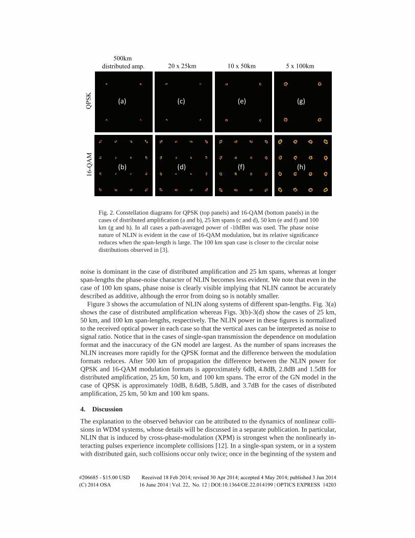
More insight as to the significance of the span-length can be extracted from Fig. 2 whichshows the received constellations in a 500 km system for QPSK (top panels) and 16-QAM(bottom panels) transmission. The first column of panels from the left [Figs. 2(a) and 2(b)]correspond to the case of distributed amplification, the second column of panels [Figs. 2(c) and2(d)] correspond to 25 km spans, the third column of panels [Figs. 2(e) and 2(f)] correspondto 50 km spans and the case of 100 km spans is shown in the rightmost panels [Figs. 2(g) and2(h)]. Here and in the figures that follow, the launched powers were selected such that the path-averaged power per-channel was -10dBm in all cases (input power of -7.7dBm, -5.9dBm and-3.3dBm, for 25 km, 50 km, and 100 km spans, respectively). Use of a constant path-averagedpower is customary when comparing systems with different span lengths [11], and the valueof -10dBm was found to be roughly optimal from the standpoint of capacity maximizationin the distributed amplification case [8]. As can be seen in Fig. 1, the comparison betweenmodulation formats is practically independent of the launched optical power. Consistently withthe predictions in [6], the phase noise is negligible in the case of QPSK transmission, and theconstellation points are nearly circular for all span-lengths. With 16-QAM modulation, phase-


500km distributed amp. 20 x 25km 10 x 50km 5 x 100km

16-Q

AM

QPS

K

(g)(c)

(d)

(e)

(f)

(g)

(h)

(c)

(d)(b)

(a)

Fig. 2. Constellation diagrams for QPSK (top panels) and 16-QAM (bottom panels) in thecases of distributed amplification (a and b), 25 km spans (c and d), 50 km (e and f) and 100km (g and h). In all cases a path-averaged power of -10dBm was used. The phase noisenature of NLIN is evident in the case of 16-QAM modulation, but its relative significancereduces when the span-length is large. The 100 km span case is closer to the circular noisedistributions observed in [3].

noise is dominant in the case of distributed amplification and 25 km spans, whereas at longerspan-lengths the phase-noise character of NLIN becomes less evident. We note that even in thecase of 100 km spans, phase noise is clearly visible implying that NLIN cannot be accuratelydescribed as additive, although the error from doing so is notably smaller.

Figure 3 shows the accumulation of NLIN along systems of different span-lengths. Fig. 3(a)shows the case of distributed amplification whereas Figs. 3(b)-3(d) show the cases of 25 km,50 km, and 100 km span-lengths, respectively. The NLIN power in these figures is normalizedto the received optical power in each case so that the vertical axes can be interpreted as noise tosignal ratio. Notice that in the cases of single-span transmission the dependence on modulationformat and the inaccuracy of the GN model are largest. As the number of spans increases theNLIN increases more rapidly for the QPSK format and the difference between the modulationformats reduces. After 500 km of propagation the difference between the NLIN power forQPSK and 16-QAM modulation formats is approximately 6dB, 4.8dB, 2.8dB and 1.5dB fordistributed amplification, 25 km, 50 km, and 100 km spans. The error of the GN model in thecase of QPSK is approximately 10dB, 8.6dB, 5.8dB, and 3.7dB for the cases of distributedamplification, 25 km, 50 km and 100 km spans.

4. Discussion

The explanation to the observed behavior can be attributed to the dynamics of nonlinear colli-sions in WDM systems, whose details will be discussed in a separate publication. In particular,NLIN that is induced by cross-phase-modulation (XPM) is strongest when the nonlinearly in-teracting pulses experience incomplete collisions [12]. In a single-span system, or in a systemwith distributed gain, such collisions occur only twice; once in the beginning of the system and


QPSK

16-QAM

GN-model

(d)

100km span-length

10

45-

40-

35-

30-

-25

Number of spans521

50-

QPSK

16-QAM

GN-model

(b)

10

50-

45-

40-

35-

-30

52155-

20

25km span-length

QPSK

16-QAM

50km span-lengthGN-model

(c)

10

50-

45-

40-

35-

-30

Number of spans521

55-

Nor

mal

ized

pow

er [d

B]

Number of spans

QPSK

16-QAM

Distributed amp.GN-model

(a)

1000

50-

45-

40-

35-

-30

Length [km]500200100

55-N

orm

aliz

ed p

ower

[dB

]

Fig. 3. Accumulation of the NLIN power (normalized to the received power) with the num-ber of spans. Figure a corresponds to the case of distributed amplification whereas figuresb,c and d correspond to the cases of 25 km, 50 km, and 100 km span-lengths, respectively.The solid lines show the theoretical results given by Eq. (1) and the dots represent simula-tions. The red dashed curve represents the SON, or equivalently the GN model result.

again at its end. In a multi-span system with lumped amplification incomplete collisions occurat every point of power discontinuity, namely at the beginning of every amplified span. Incom-plete collisions taking place at different locations, produce NLIN contributions of independentphase and therefore, when the NLIN is dominated by incomplete collisions, it appears moreisotropic in phase-space and its distribution becomes closer to Gaussian. The relative signifi-cance of incomplete collisions is determined mainly by two factors; the number of incompletecollisions (which grows with the number of spans), and the magnitude of power discontinuity(increases with span length). For a fixed length link, when the number of spans is so large thatattenuation within the span is negligible, the power discontinuity at the amplifier sites vanishesand the system becomes equivalent to a distributed gain system, where only two incomplete col-lisions occur (at the beginning and at the end of the entire link). As the span length increases,the power discontinuity at the amplifier locations grows and the overall significance of incom-plete collisions increases. This explains the fact that in Fig. 2 the 16-QAM constellation spotsappear more and more circular as the span length increases from 0 (distributed amplification) to100 km. When the span-length increases further, to the extent that it becomes much longer thanthe fiber’s effective length (1/α ∼ 20 km in most fibers), the growth in the power discontinu-ity becomes negligible, but the number of incomplete collisions continues to decrease with thenumber of spans, until eventually, in a single-span link (where only one incomplete collisionoccurs at the link’s beginning) the non-Gaussianity of NLIN reappears and the deviation fromthe GN model is very significant. This point can be seen in Figs. 3(b)–3(d), where the NLIN


100

0.5

/0.6

0.7

0.8

0.9

1

101

102

103

Number of spans10

1

0.5

0.6

0.7

0.8

0.9

1

102

103

104

Length [km]

0.4

50km Span-length

25km span-length

100km span-length

distributed amp.

Fig. 4. The importance of incomplete collisions is reflected in the ratio between the FONand SON coefficients χ2/χ1. When incomplete collisions dominate χ2/χ1 � 1, and whentheir contribution is small (as occurs in single span, or distributed gain systems) χ2/χ1 ∼ 1.In (a) The total link-length is held fixed at 500 km. In (b) the span length is kept constant.In both Figs. (a) and (b), the dashed curve corresponds to distributed amplification.

variance is shown as a function of the number of spans and the span-length is kept constant.The error in the GN model is always largest in a single-span link, and reduces considerablywith the number of spans in the case of lumped amplification.

Figure 4 summarizes these ideas by showing the ratio χ2/χ1 as a function of the number ofspans in a fixed-length system [Fig. 4(a)], and as a function of system length [Fig. 4(b)]. Whenincomplete collisions dominate so that the NLIN approaches a circular Gaussian distributionand the significance of phase-noise reduces, χ2/χ1 � 1 and the NLIN variance is dominatedby the SON contribution (the GN model). In Fig. 4(a) the deviation from the GN model is seento be largest (χ2/χ1 ∼ 1) in the single-span case, and when the number of spans is so largethat the scheme approaches the conditions of distributed amplification. When the span-lengthis fixed, as in Fig. 4(b), the ratio χ2/χ1 reduces with the length of the link, with the highest rateof reduction occurring when the span-length is long so that the power discontinuity is largest.

Another interesting aspect of the nonlinear dynamics is revealed in the context of the effectof signal pre-dispersion. One of the most central claims made in [2–4, 7] is that signal Gaus-sianity, which is crucial for the validity of the GN model, follows from the accumulated effectof chromatic dispersion, and hence the large inaccuracy of the GN model in the first few spansof a WDM system was attributed to the fact that the signal is not sufficiently dispersed. Indeed,in [4] it has been demonstrated that in the presence of very aggressive pre-dispersion, the NLINvariance is accurately described by the GN model even in the very first few spans (where with-out pre-dispersion the inaccuracy of the GN model is largest). In our understanding the role ofdispersion in this context has been misconstrued. While it is true that significant pre-dispersionreduces the GN model’s inaccuracy in the first span, as shown in [4], it is not the absence of suf-ficient dispersion that explains the GN model’s inaccuracy. Here we present an alternative viewat the role of pre-dispersion. We plot in Fig. 5 the NLIN variance as a function of system length,once in the case of distributed amplification and once in the case of lumped amplification with100km spans. In both cases the signals were pre-dispersed by 8500 ps/nm — equivalent to a500 km long link. Notice that indeed pre-dispersion improves the accuracy of the SON termrepresenting the GN model in the first few spans. However, when the link becomes longer andthe accumulated dispersion exceeds the amount of pre-dispersion assigned to the signal, the de-viation from the GN-model increases and eventually, the simulated NLIN variance approachesthe same value that it has without pre-dispersion. This behavior is seen to be in clear contrast to


QPSK

16-QAM

GN-model

100km span-length8500ps/nm pre-disp.

(b)

1040-

35-

30-

-25

Number of spans521

QPSK

16-QAM

GN-model

Distributed amp.8500ps/nm pre-disp.

Nor

mal

ized

pow

er [d

B]

(a)

1000

40-

35-

-30

Length [km]500200100

45-

Fig. 5. The effect of pre-dispersion. Accumulation of the NLIN power (normalized to thereceived power) with the number of spans. Figures a and b correspond to distributed am-plification and span-length of 100 km, respectively, where pre-dispersion of 8500 ps/nmwas applied to the injected pulses. The solid lines show the theoretical results given byEq. (1) and the dots represent simulations. The red dashed curve represents the SON, orequivalently the GN model result.

the interpretation of [2–4,7]. If the pre-dispersed signals are Gaussian enough at the end of thefirst span so as to satisfy the assumptions of the GN model, how come they are less Gaussianfurther along the system given that the accumulated dispersion increases monotonically? Ourown interpretation to this behavior relies once again on the time domain picture of pulse colli-sions. When the temporal spreading of the launched pulses is larger than the walk-off betweenchannels, all collisions become incomplete, and for the same reasons that we explained earlierthe GN model becomes more accurate. Nonetheless, when the system length increases to theextent that the inter-channel walk-off becomes large enough to accommodate full collisions,the deviation from the GN result reappears once again.

When examining the situation in the frequency domain picture, pre-dispersion implies rapidphase variations in the interfering channel’s spectrum (i.e. variations in the phase of g(ω) inthe notation of [6]). While the SON coefficient χ1 is not affected by the spectral phase, theFON coefficient χ2 reduces considerably in this situation, since the fourth-order correlationterms (Eq. 24 in [6]) lose coherence. We note however, that since with all relevant modulation

formats, the quantity 〈|b|4〉〈|b|2〉2 − 2 is negative, the reduction of χ2 through pre-dispersion always

leads to an increase in the NLIN variance and is therefore undesirable.

5. Conclusions

We have shown that the previously unexplained dependence of the NLIN variance on pre-dispersion, modulation format and on the number of amplified spans, is accounted for by theFON term, which follows from the correct treatment of the signal’s statistics [6]. Excellentagreement between theory and simulations has been demonstrated in all of our simulations,suggesting that in the range of parameters that we have tested, the inclusion of additional cor-rection terms, which were presented in [7] is not necessary. The relative magnitude of the FONterm is largest in single span systems, or in systems using distributed amplification, and it re-duces notably in the case of lumped amplification with a large number of spans. Similarly, therelative significance of phase noise (which is included both in the SON and the FON terms) islargest in single span systems, or in systems with distributed amplification, although it remainssignificant in all the cases that we have tested.


Appendix: Computation of χ1 and χ2

The extraction of the analytical curves in Figs. 1 and 3 –5 relies on the computation of theSON and FON coefficients χ1 and χ2, which requires summation over three and five indices,respectively. Multi-dimensional summations are extremely inefficient in brute-force computa-tion, and hence we have adopted the Monte-Carlo integration method [13] for evaluating thesequantities. We provide a code (written in Matlab) that computes χ1, χ2 (using Eqs. (26) and(27) of [6] including receiver matched filtering that removes products that fall outside of the re-ceived channel bandwidth), and allows the evaluation of the implied NLIN variance accordingto Eq. (1). The program also evaluates the relative error in the computed NLIN variance, wherein all of the numerical curves presented in this paper the number of integration points N waslarge enough to ensure that the relative error was well under 1%.

For the reader’s convenience, in addition to providing the tools for reproducing the curvespresented in this paper, we include blocks that compute the variance of nonlinear intra-channelnoise, as well as additional inter-channel terms that contribute to NLIN when the guard-bandbetween WDM channels is much smaller than the channel bandwidth, and which were firstreported in [7]. It can be easily verified that the contribution of these terms is negligible withthe typical system parameters assumed in this paper, although they may play a role in the case offuture densely spaced super-channels. The option of describing a polarization multiplexed linkis also included. The program assumes perfect Nyquist pulses and homogeneous fiber spans,but it can be readily extended to an arbitrary pulse-shape and to systems with different spanlength and fiber dispersions.

The runtime for the computation of the SON and FON coefficients χ1 and χ2 on a standardPC with an i5 processor is of the order of 0.5 seconds, whereas the computation of all (intraand inter-channel) NLIN terms is performed in less than 2 seconds. We note that polarizationmultiplexing does not affect the run-time of the code (although it more than doubles the runtimeof a full split-step simulation). A link to this code, as well as to its future upgrades, will also beposted at http://www.eng.tau.ac.il/nlin/.

function main()%% System parametersclear;clc;tic;PolMux = 0; % 0 when single polarization, 1 with polarization multiplexinggamma = 1.3; % Nonlinearity coefficient in [1/W/km]beta2 = 21; % Dispersion coefficient [psˆ2/km]alpha = 0.2; % Fiber loss coefficient [dB/km]Nspan = 5; % Number of spansL = 100; % Span length [km]PD = 0; % Pre-dispersion [psˆ2]PdBm = -2; % Average input power [dBm]BaudRate = 32; % Baud-rate [GHz]ChSpacing = 50; % Channel spacing [GHz]kur = 1.32; % Second order modulation factor <|a|ˆ4>/<|a|ˆ2>ˆ2kur3 = 1.96; % Third order modulation factor <|a|ˆ6>/<|a|ˆ2>ˆ3N = 1000000; % Number of integration points in algorithm [14]. Should

% be set such that the relative error is desirably small.

%% Monte-Carlo integrationalpha_norm =alpha/10*log(10);T=1000/BaudRate;P0 = 10ˆ((PdBm-30)/10);beta2_norm = beta2/Tˆ2;PD_norm = PD/Tˆ2;ChSpacing_norm = ChSpacing./BaudRate;


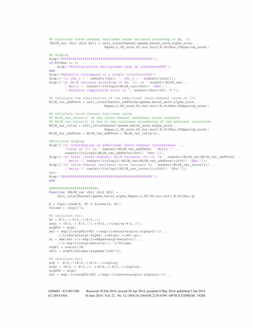
%% calculate inter-channel nonlinear noise variance according to Eq. (1)[NLIN_var chi1 chi2 Err] = calc_interChannel(gamma,beta2_norm,alpha_norm,...

Nspan,L,PD_norm,P0,kur,kur3,N,PolMux,ChSpacing_norm);

%% displaydisp('%%%%%%%%%%%%%%%%%%%%%%%%%%%%%%%%%%%%%%%%%%%%%%');if(PolMux == 1)

disp('%%%Polarization Multiplexed case is considered%%%');enddisp('%%Results correspond to a single interferer%%%')disp(['(1) chi_1 = ' num2str(chi1) ', chi_2 = ' num2str(chi2)]);disp(['(2) NLIN variance according to Eq. (1) is ' num2str(NLIN_var)...

' Watts (' num2str(10*log10(NLIN_var*1000)) 'dBm).'...' Relative computation error is ', num2str(Err*100),'%']);

%% calculate the contribution of the additional inter-channel terms of [7]NLIN_var_addTerm = calc_interChannel_addTerms(gamma,beta2_norm,alpha_norm,...

Nspan,L,PD_norm,P0,kur,kur3,N,PolMux,ChSpacing_norm);

%% calculate intra-channel nonlinear noise%% NLIN_var_intra(1) is the intra-channel nonlinear noise variance%% NLIN_var_intra(2) is due to the nonlinear broadening of the adjacent interfererNLIN_var_intra = calc_intraChannel(gamma,beta2_norm,alpha_norm,...

Nspan,L,PD_norm,P0,kur,kur3,N,PolMux,ChSpacing_norm);NLIN_var_addTerm = NLIN_var_addTerm + NLIN_var_intra(2);

%%Continue displaydisp(['(3) Contribution of additional inter-channel interference '...

'terms of [7] is ' num2str(NLIN_var_addTerm) ' Watts ('...num2str(10*log10(NLIN_var_addTerm*1000)) 'dBm)']);

disp(['(4) Total (inter-channel) NLIN variance (2)+(3) is ' num2str(NLIN_var+NLIN_var_addTerm)...' Watts (' num2str(10*log10((NLIN_var+NLIN_var_addTerm)*1000)) 'dBm)']);

disp(['(5) Intra-Channel nonlinear noise variance is ' num2str(NLIN_var_intra(1))...' Watts (' num2str(10*log10(NLIN_var_intra(1)*1000)) 'dBm)']);

toc;disp('%%%%%%%%%%%%%%%%%%%%%%%%%%%%%%%%%%%%%%%%%%%%%%');end

%%%%%%%%%%%%%%%%%%%%%%%%%function [NLIN_var chi1 chi2 Err] = ...

calc_interChannel(gamma,beta2,alpha,Nspan,L,PD,P0,kur,kur3,N,PolMux,q)

R = 2*pi*(rand(4, N)-0.5*ones(4, N));Volume = (2*pi)ˆ4;

%% calculate chi1w0 = R(1,:)-R(2,:)+R(3,:);arg1 = (R(2,:)-R(3,:)).*(R(2,:)+2*pi*q-R(1,:));argPD1 = arg1;ss1 = exp(1i*argPD1*PD).*(exp(1i*beta2*arg1*L-alpha*L)-1)...

./(1i*beta2*arg1-alpha).*(w0<pi).*(w0>-pi);s1 = abs(ss1.*(1-exp(1i*Nspan*arg1*beta2*L))...

./(1-exp(1i*arg1*beta2*L))).ˆ2/Volume;avgF1 = sum(s1)/N;chi1 = avgF1*Volume*(4*gammaˆ2*P0ˆ3);

%% calculate chi2w3p = -R(2,:)+R(4,:)+R(3,:)+2*pi*q;arg2 = (R(2,:)-R(3,:)).*(R(4,:)-R(1,:)+2*pi*q);argPD2 = arg2;ss2 = exp(-1i*argPD2*PD).*(exp(-1i*beta2*arg2*L-alpha*L)-1)...


./(-1i*beta2*arg2-alpha).*(w3p>-pi+2*pi*q).*(w3p<pi+2*pi*q);s2 = (1-exp(1i*Nspan*arg1*beta2*L))./(1-exp(1i*arg1*beta2*L)).*ss1...

.*(1-exp(-1i*Nspan*arg2*beta2*L))...

./(1-exp(-1i*arg2*beta2*L)).*ss2/Volume;avgF2 = real(sum(s2))/N;chi2 = avgF2*Volume*(4*gammaˆ2*P0ˆ3);

%% calculate NLINNLIN_var = chi1+(kur-2)*chi2;if(PolMux == 1)

NLIN_var = (9/8)ˆ2*16/81*(NLIN_var+2*chi1/4+(kur-2)*chi2/4);end

%% calculate the root mean square relative errorif(PolMux == 0)

Err = (sum((s1-avgF1+(kur-2)*(real(s2)-avgF2)).ˆ2).../(N-1))ˆ.4/(avgF1+(kur-2)*avgF2)/sqrt(N);

elseErr = (sum(((9/8)ˆ2*16/81*(6/4*(s1-avgF1)+5/4*(kur-2)*...

(real(s2)-avgF2))).ˆ2)/(N-1))ˆ.4/((9/8)ˆ2*16/81*...(6/4*avgF1+5/4*(kur-2)*avgF2))/sqrt(N);

end

end

%%%%%%%%%%%%%%%%%%%%%%%%%function [NLIN_var] = calc_interChannel_addTerms(gamma,beta2,alpha,...

Nspan,L,PD,P0,kur,kur3,N,PolMux,q)

R = 2*pi*(rand(4, N)-0.5*ones(4, N));

%% calculate X21w0 = R(1,:)-R(2,:)+R(3,:)+2*pi*q;arg1 = (R(2,:)-R(3,:)-2*pi*q).*(R(2,:)-R(1,:));argPD1 = arg1;ss1 = exp(1i*argPD1*PD).*(exp(1i*beta2*arg1*L-alpha*L)-1)...

./(1i*beta2*arg1-alpha).*(w0<pi).*(w0>-pi);s1 = abs(ss1.*(1-exp(1i*Nspan*arg1*beta2*L))./(1-exp(1i*arg1*beta2*L))).ˆ2;X21 = sum(s1)*(gammaˆ2*P0ˆ3)/N;

%% calculate X22w1 = R(1,:)-R(2,:)+R(4,:);arg2 = (w1-R(3,:)-2*pi*q).*(R(2,:)-R(1,:));argPD2 = arg2;ss2 = exp(-1i*argPD2*PD).*(exp(-1i*beta2*arg2*L-alpha*L)-1)...

./(-1i*beta2*arg2-alpha).*(w1<pi).*(w1>-pi);s2 = (1-exp(1i*Nspan*arg1*beta2*L))./(1-exp(1i*arg1*beta2*L)).*ss1...

.*(1-exp(-1i*Nspan*arg2*beta2*L))./(1-exp(-1i*arg2*beta2*L)).*ss2;X22 = real(sum(s2))*(gammaˆ2*P0ˆ3)/N;

%% calculate X23w2 = R(1,:)+R(2,:)-R(3,:)-2*pi*q;arg1 = (R(3,:)+2*pi*q-R(2,:)).*(R(3,:)+2*pi*q-R(1,:));argPD1 = arg1;ss3 = exp(1i*argPD1*PD).*(exp(1i*beta2*arg1*L-alpha*L)-1)...

./(1i*beta2*arg1-alpha).*(w2<pi).*(w2>-pi);s3 = abs(ss3.*(1-exp(1i*Nspan*arg1*beta2*L))./(1-exp(1i*arg1*beta2*L))).ˆ2;X23 = sum(s3)*(gammaˆ2*P0ˆ3)/N;

%% calculate X24w3 = R(1,:)-R(4,:)+R(2,:);arg2 = (R(3,:)+2*pi*q-R(4,:)).*(R(3,:)+2*pi*q-w3);


argPD2 = arg2;ss4 = exp(-1i*argPD2*PD).*(exp(-1i*beta2*arg2*L-alpha*L)-1)...


.*(1-exp(-1i*Nspan*arg2*beta2*L))./(1-exp(-1i*arg2*beta2*L)).*ss4;X24 = real(sum(s4))*(gammaˆ2*P0ˆ3)/N;

%% calculate NLINNLIN_var = 4*X21+4*(kur-2)*X22+2*X23+(kur-2)*X24;if(PolMux == 1)

NLIN_var = (9/8)ˆ2*16/81*(NLIN_var+2*X21+(kur-2)*X22+X23+0*(kur-2)*X24);end

end

%%%%%%%%%%%%%%%%%%%%%%%%%function [NLIN_var] = ...

calc_intraChannel(gamma,beta2,alpha,Nspan,L,PD,P0,kur,kur3,N,PolMux,q)

if(exist('q')==0) q = 0; end;R = 2*pi*(rand(5, N)-0.5*ones(5, N));

%% calculate X1w0 = R(1,:)-R(2,:)+R(3,:);argInB = (w0<pi).*(w0>-pi);argOutB = (w0<pi+2*pi*q).*(w0>-pi+2*pi*q);arg1 = (R(2,:)-R(3,:)).*(R(2,:)-R(1,:));argPD1 = arg1;ss1 = exp(1i*argPD1*PD).*(exp(1i*beta2*arg1*L-alpha*L)-1)...

./(1i*beta2*arg1-alpha);s1 = abs(ss1.*(1-exp(1i*Nspan*arg1*beta2*L))./(1-exp(1i*arg1*beta2*L))).ˆ2;X1 = [sum(s1.*argInB) sum(s1.*argOutB)]*(gammaˆ2*P0ˆ3)./N;

%% calculate X0s0 = ss1.*(1-exp(1i*Nspan*arg1*beta2*L))./(1-exp(1i*arg1*beta2*L));X0 = [abs(sum(s0.*argInB)/N).ˆ2 abs(sum(s0.*argOutB)/N).ˆ2]*(gammaˆ2*P0ˆ3);

%% calculate X2w1 = -R(2,:)+R(4,:)+R(3,:);arg2 = (R(2,:)-R(3,:)).*(R(4,:)-R(1,:));argPD2 = arg2;ss2 = exp(-1i*argPD2*PD).*(exp(-1i*beta2*arg2*L-alpha*L)-1)...


.*(1-exp(-1i*Nspan*arg2*beta2*L))./(1-exp(-1i*arg2*beta2*L)).*ss2;X2 = [real(sum(s2.*argInB)) real(sum(s2.*argOutB))]*(gammaˆ2*P0ˆ3)./N;

%% calculate X21w2 = R(4,:)-R(1,:)-R(3,:);arg2 = (R(2,:)-R(4,:)).*(R(2,:)-w2);argPD2 = arg2;ss2 = exp(-1i*argPD2*PD).*(exp(-1i*beta2*arg2*L-alpha*L)-1)...



%% calculate X3w3 = R(1,:)-R(2,:)+R(4,:)+R(3,:)-R(5,:);arg3 = (R(4,:)-R(5,:)).*(R(4,:)-w3);argPD3 = arg3;ss3 = exp(-1i*argPD3*PD).*(exp(-1i*beta2*arg3*L-alpha*L)-1)...




%% calculate NLINNLIN_var = 2*X1+(kur-2)*(4*X2+X21)+(kur3-9*kur+12)*X3-(kur-2)ˆ2*X0;if(PolMux == 1)

NLIN_var = (9/8)ˆ2*16/81*(NLIN_var+X1+(kur-2)*X2);end

end

Acknowledgments

The authors would like to acknowledge financial support from the Israel Science Foundation(grant 737/12). Ronen Dar would like to acknowledge the support of the Adams Fellowship ofthe Israel Academy of Sciences and Humanities, the Yitzhak and Chaya Weinstein ResearchInstitute, and the Feder Family Award.


accumulation of nonlinear interference noise in fiber-optic systems

Documents