accessibility to alcohol outlets and alcohol consumption

© Copyright Victorian Health Promotion Foundation 2011

Published in December 2011 by the Victorian Health Promotion Foundation (VicHealth)

PO Box 154 Carlton South, VIC 3053 Australia

ISBN: 978-1-921822-43-8 Publication number: K-034-ATUV

Suggested citation Accessibility to alcohol outlets and alcohol consumption: Findings from VicLANES. Victorian Health Promotion Foundation (VicHealth), Carlton, Australia.

Accessibility to alcohol outlets and alcohol consumption: Findings from VicLANES

Professor Anne Kavanagh and Ms Lauren Krnjacki

Centre for Women’s Health, Gender and Society

Melbourne School of Population Health

The University of Melbourne

2 of 28

Table of contents

1. Summary of project 3

2. Plain language summary 4

3. Background 5

3.1 Access to alcohol outlets selling products for off‐premise consumption 6

3.2 Price and availability of alcoholic beverages 6

3.3 VicLANES 7

4. Methods 8

4.1 Selection of VicLANES areas and participants 8

4.2 Collection of environmental data 8

4.3 Collection of individual data 9

4.4 Variables used in analysis 9

4.5 Analytical approach 12

5. Results ................................................................................................................ 13

5.1 Prevalence of harms 13

5.2 Demographics and alcohol consumption 13

5.3 Distribution of alcohol environment measures 14

5.4 Bivariate associations between alcohol environment and alcohol consumption 14

5.5 Multilevel regression analyses 16

6. Discussion 21

6.1 Discussion of findings 21

6.2 Strengths and limitations 22

7. Recommendations 24

8. References 25

9. Appendix 27

9.1 Alcohol consumption and demographics 27

9.2 Methodological issues 28

3 of 28

1. Summary of project

The Victorian Lifestyle and Neighbourhood Environment Study (VicLANES) was conducted in

late 2003. As part of that study, detailed information was collected from over 2500 participants

in 50 census collector districts (CCD) in Melbourne about their alcohol consumption patterns.

An audit was conducted on all outlets selling liquor for off‐premise consumption, and the

availability and price of 70 different alcoholic beverages were recorded. Using these data, we are

able to assess the extent to which access to alcohol stores and the range and price of alcoholic

beverages within stores influences whether individuals drink at levels associated with harm. In this

report, we overview the current literature, present the main findings from the analysis of these

data and make some recommendations for future research and policy.

The findings presented in this report have also been written up as journal articles that are

currently under review or in preparation.

Objectives

In this report we address two key questions:

• Does accessibility to alcohol outlets close to home increase harmful alcohol consumption?

• Do the price and availability of a range of alcoholic beverages in alcohol outlets close to

home increase harmful alcohol consumption?

Funding

This analysis was funded by a VicHealth grant of $13,505.92, plus GST

4 of 28

2. Plain language summary

Using data collected in VicLANES of 2,334 adults living in 49 small areas in metropolitan

Melbourne, we investigated whether access to alcohol outlets that sold liquor for consumption

off premises influenced whether individuals consumed alcohol at levels associated with short‐

or long‐term harm, as well as the frequency of consumption. We used four measures of access:

• density: the number of stores within a one‐kilometre road network distance of

respondents’ homes

• proximity: the distance from a respondent’s home to their closest store measured

along a road network

• availability: the number of beverages stocked in the closest store out of a possible 70

items audited

• price: the price of a commonly stocked basket of beverages in the closest store.

We found that having access to a greater number of outlets increased the risk of drinking at levels

associated with short‐term harm. Having eight or more stores within in a one‐kilometre network

distance of respondents’ home more than doubled the odds of consuming alcohol at levels

associated with short‐term harm at least weekly. We found some limited evidence that increased

availability of a range of alcoholic beverages in the stores closest to respondents’ homes actually

reduced the risk of consuming at levels associated with long‐term harm.

We recommend that policy makers consider the introduction of interventions to restrict the

number of outlets in areas. We also recommend that policy interventions to reduce alcohol

consumption, such as legislation limiting the number of new licenses or increasing the price of

beverages, be rigorously evaluated. We note that we did not collect data on premises that sell

alcohol for consumption on site, and recommend that this could be an area of future research.

The findings of the analysis on the density and proximity of alcohol outlets and consumption at

levels associated with harm has been published previously (see Kavanagh AM, Kelly MT, Krnjacki L,

Thornton L, Jolley D, Subramanian SV, Turrell G, Bentley RJ. Access to alcohol outlets and harmful

alcohol consumption: a multi‐level study in Melbourne, Australia. Addiction. 2011

Oct;106(10):1772‐9)

5 of 28

3. Background

Alcohol use is associated with a wide range of health and social problems, and thus there is considerable

interest nationally and internationally to develop interventions to reduce the consumption of

alcohol at levels associated with harm (National Preventative Health Taskforce 2008; World Health

Organization 2007). The consequences of binge drinking, or drinking a large number of drinks on one

occasion, include injuries, assaults and self‐harm. Drinking at high levels over the longer term is associated

with an increased risk of chronic diseases, such as liver disease, pancreatitis and cardiovascular

disease (National Health and Medical Research Council 2001, 2007; World Health Organization 2007).

Although there is considerable research demonstrating individual predictors of hazardous alcohol

use, including being male (Australian Institute of Health and Welfare 2007), low socioeconomic position

(Menvielle et al. 2007), younger age (Australian Institute of Health and Welfare 2007; Hibell et al. 2004)

and Indigenous status (Australian Institute of Health and Welfare 2007), there has been less

research on the impact of accessibility to alcohol outlets on consumption. The National Alcohol Strategy

2006–2011 (National Alcohol Strategy 2006‐2011 2006) identifies restrictions on the economic and physical

availability of alcohol as ways to potentially reduce harmful drinking behaviours. It recommends that

future research investigates whether reducing geographic and economic access to alcohol decreases the

risk of harmful alcohol consumption. This evidence could then be used to inform future research in the field.

Developed countries, such as Australia, have either introduced, or are considering, legislation to restrict

the number of alcohol outlets, particularly those selling liquor for off‐premise consumption (Liquor Control

Advisory Council 2007). However, there is little evidence to support this strategy, particularly from

countries other than the USA (Chikritzhs et al. 2007).

There have been a number of price‐related policy initiatives in Australia, France, Switzerland, Germany and

Denmark (Anderson & Baumberg 2006; The Honourable Nicola Roxon MP) that have been introduced, with

the intent of reducing risk of harmful alcohol consumption. For example, in 2008, the Australian

Government increased the tax on premixed spirits, and in 2009, reported a subsequent decline in the

sale of these alcoholic products (The Honourable Nicola Roxon MP). We briefly review the evidence

on access to alcohol environments and consumption of alcohol at levels associated with harm.

First, we discuss research findings about access to alcohol outlets and harmful consumption.

Second, we summarise findings on the effects of price and availability of alcohol within stores

on consumption.

6 of 28

3.1 Access to alcohol outlets selling products for off‐premise consumption

The relationship between access to off‐premise alcohol outlets and consumption has generated

mixed evidence. Some studies have found higher levels of drinking in areas with a higher density

of off‐premise outlets (Kypri et al. 2008; Schonlau et al. 2008). A study conducted by Livingston

et al. (Livingston, Laslett & Dietze 2008) in Melbourne found that the density of off‐site alcohol

outlets was associated with an increased prevalence of high‐risk drinking in young adults

between the ages of 16 and 24 years. In New Zealand, a national study found that the density

of outlets was associated with increased binge drinking and alcohol‐related harm (Connor

et al. 2010). Pollack et al. (Pollack et al. 2005); however, did not find evidence to support

an association between density and consumption in the USA. Two studies examined whether

residents’ proximity to the nearest alcohol outlet influenced consumption, but neither study

found evidence to support an association (Pollack et al. 2005; Scribner, Cohen & Fisher 2000).

Studies to date have had considerable limitations, particularly in relation to how exposure to

alcohol outlets has been defined. The most frequent measure of outlet density is the absolute

number of outlets in a specified area (Chen, Grube & Gruenewald 2010; Gruenewald, Johnson

& Treno 2002; Livingston, Laslett & Dietze 2008; Nelson 2008; Pollack et al. 2005). This approach

best represents the exposure of residents at the centre of an area, with misclassification more

likely for residents closest to the boundary (Hewko, Smoyer‐Tomic & Hodgson 2002; Matisziw,

Grubesic & Wei 2008). A more accurate reflection of the number of stores near an individual’s

residence is the number of stores that fall within a specified distance from the residence. Road

network distances provide better measures than Eucidean or straight‐line measures of access.

Previous studies have not used this approach, with the exception of Schonlau et al., who found a

stronger association between alcohol density and consumption when network distance was used,

as compared to the absolute number of outlets in census tracts (Schonlau et al. 2008).

3.2 Price and availability of alcoholic beverages

There is a large body of literature that addresses the relationship between alcohol price and

consumption; however, the majority of these studies have been ecological and have assessed the

relationship between the price (or taxes as a proxy for price) of beverages and consumption. A

recent systematic review and meta‐analysis of this literature found that alcohol prices and taxes

7 of 28

are related inversely to drinking (Wagenaar, Salois & Komro 2009). We are unaware of any

studies that have used a multilevel study design to assess the relationship between the price of

beverages and consumption. In VicLANES, we have the capacity to identify the price of a range of

beverages for stores that are closest to home.

3.3 VicLANES

This study uses data from VicLANES, conducted in Melbourne, Australia in 2003. The study was

approved by the La Trobe University Human Research Ethics Committee. The approval included

approval for access to the Australian electoral roll, which lists the name, residential address and

age of each registered voter. The aim of VicLANES was to examine the importance of individual

and area‐level characteristics in relation to three health behaviours: household food purchasing,

physical activity and alcohol consumption (Kavanagh et al. 2007).

8 of 28

4. Methods

We discuss how we collected data on individuals and alcohol environments.

4.1 Selection of VicLANES areas and participants

VicLANES used a two‐stage cluster design to select areas and individuals.

The first stage involved the sampling of 4170 CCD from the 21 innermost local government areas

(LGA) in Melbourne. These LGA were situated in an approximately 20‐kilometre radius from the

central business district of Melbourne. CCD are used by the Australian Bureau of Statistics to

collect population census data, and were the smallest geographic area defined in the Australian

Standard Geographical Classification in 2001 (Australian Bureau of Statistics 2006). CCD in the

sampling area had an average of 557 residents, and a mean size of 0.34 square kilometres. All

CCD located within the LGA were ranked according to the proportion of households with a

weekly pretax income of less than $400/week (low‐income households). CCD were

subsequently stratified into septiles based on this ranking, and a random sample of 50 CCD

from the highest (17 CCD), middle (16 CCD) and lowest (17 CCD) strata were selected.

4.2 Collection of environmental data

Collection of data on location of stores

The names and addresses of all alcohol outlets in Victoria that sold alcohol for consumption off

premises were obtained from the Victorian Liquor Licensing Authority (Liquor Licensing Victoria

2002), and a field audit was conducted to verify the accuracy and completeness of the list. We

geocoded all alcohol outlets that sold liquor that could be consumed off premises within a

catchment area of 2‐kilometres’ Euclidian distance of the centroid of the selected CCD. This

catchment area captured all outlets within a 1‐kilometre road network distance of all

participants’ homes.

In‐store audits of price and availability

Trained field auditors attended all stores to confirm the store was trading and selling liquor for

off‐site consumption. They also conducted a stocktake of presence and price of 70 different alcoholic

beverages.

9 of 28

4.3 Collection of individual data

Sampling of individuals and response rate

We used the Australian electoral roll to identify all households in the selected CCD who had at least one

adult aged between 18 and 75 years (it is compulsory for all persons aged 18 and over to vote, and

it is estimated that 97.7 per cent of persons eligible to vote are enrolled (Australian Electoral

Commission 2005). We randomly selected one person in a household when there was more than one

eligible adult. Four thousand and five individuals were sampled. A postal survey was used to collect

individual and household data. A tailored design method for mail surveys was used in order to

maximise response rates to the postal survey (Dillman 2000). Valid responses were obtained from

2,349 respondents, equating to a response rate of 58.7 per cent (54.6 per cent in the most disadvantaged

septile, 59 per cent in the middle septile and 62.1 per cent in the most advantaged septile).

Participation rates were inversely associated with area disadvantage, with high SES strata areas

having higher rates than mid and low SES strata areas. We obtained census data for the included

CCD, and our sample had a lower proportion of households in the lowest quintile of income, persons with

no post‐school qualification, blue collar workers, men and persons aged 18–24 years (data not shown).

4.4 Variables used in analysis

Outcome: alcohol consumption

The questions relating to alcohol consumption were based on the 2001 National Household Drug Survey

(Australian Institute of Health and Welfare 2002). In the postal questionnaire, participants were

asked if they ever consumed alcohol. If they responded ‘yes’, they were then asked:

• the frequency with which they consumed an alcoholic drink in the last 12 months, with eight

response categories: everyday, five to six days/week, three to four days/week, one to two

days/week, two to three days a month, about one day a month, less often and no longer drink

• how many drinks they usually consumed per drinking occasion, with six response categories:

13 or more, 11–12, seven to 10, five to six, three to four and one to two drinks

• the frequency with which they consumed alcohol at levels associated with short‐term harm.

Male respondents were asked how many times in the past year they consumed more than six

standard drinks in a day, and females were asked the frequency with which they consumed

more than four standard drinks. The response to this question included the same eight

categories as the first question.

10 of 28

One standard drink was defined as 10 grams of alcohol, in accordance with the Australian National

Health and Medical Research Councils (NHMRC) alcohol guidelines (National Health and Medical

Research Council 2001). Pictures of typical serving sizes showing the equivalent number of

standard drinks were used to help participants estimate their consumption. We used the NHMRC

alcohol consumption guidelines (National Health and Medical Research Council 2001) to derive

the outcome variables of harmful consumption outlined below:

Short‐term harm (weekly and monthly)

Short‐term harm was defined as more than six drinks for men, and more than four drinks for

women. We computed two short‐term harm variables, which referred to drinking at levels

associated with short‐term harm, at least once per week (short‐term harm weekly), or at least

once per month (short‐term harm monthly).

Long‐term harm

Long‐term harm was computed by multiplying the responses to the first question with the

responses to the second question, with mid‐points used when the category included a range.

Long‐term harm was defined as 29 standard drinks or more per week for men, and 15 drinks

or more per week for women.

Frequent consumption

We also derived a variable to represent the frequency of consumption, which was coded

as 0=drink less often than five days per week, and 1=drinks on five or more days per week. This

frequency of the consumption variable captured regular consumption, but did not necessarily

represent frequent consumption at levels associated with harm.

Exposures: Access to alcohol

The locations of participants’ homes were geocoded using ArcGIS version 9.3 (ESRI, Redlands,

California, United States of America). There was a 100 per cent match rate, because the address

data were obtained from the Australian electoral roll and were not self‐reported. With regards to

alcohol outlets, we again achieved a 100 per cent match rate, as the address data were sourced

from Liquor Licensing Victoria, who requires a valid address prior to the issue of a license. For the

network distance analysis, the types of roads were not considered, because we were interested in

11 of 28

driving distance, not driving time, which is where a consideration of road infrastructure and

conditions are more important. Our road network analysis was configured so that restrictions

were placed on one‐way roads, and U‐turns were permitted.

We did not include pedestrian walkways and alleys in the route options, as we were interested

in the usual minimum travel distance by motor vehicle. Information obtained in the audit

showed that all areas sampled had a reasonable quality of footpaths, so pedestrians would have

had the option to travel along the same routes as motor vehicles.

Density

Density was calculated by counting the number of outlets within a 1‐kilometre road network

distance from the respondents’ homes. We modelled density separately, as both a continuous

and a categorical variable, to determine if there were potential threshold effects. Density was

categorised as: no outlets, one outlet, two outlets, three to four outlets, five to seven outlets and

eight or more outlets.

Proximity

Proximity was the road distance (in kilometres) from the respondents’ homes to the nearest alcohol

outlet. We modelled proximity as both a continuous and categorical variable to determine if there were

potential threshold effects. Proximity was classified into the following categories: <0.4 kilometres, 0.4 to

<0.8 kilometres, 0.8 to <1.2 kilometres and 1.2 or more kilometres.

Availability

Availability was defined as the number of available beverages in the audited stores (i.e. number could

range from 1 to 70) that was closest to an individual’s home. Availability was classified into the following

categories: <40 items, 40–49 items, 50–59 items and 60 or more items.

Price

Price was estimated by calculating the price of a ‘basket’ of common items. These items represented

the most commonly‐available items across the different categories of alcoholic beverages (i.e. spirits, wine,

beer). These items were: Jack Daniels whiskey, Stolichnaya vodka, Penfold’s fortified wine, Four Sisters

white wine, Wolf Blass red wine, Yellowglen sparkling, Carlton Cold beer, Cascade beer and Lemon

Ruski (premix). There was a large amount of missing data, as not all items in the ‘basket’ were available

12 of 28

in all stores; however, we estimated the price of the full basket using multiple imputation (see the

Appendix for further information on the statistical methods). Price was classified into categories of:

<$130, $130 to <$135, $135 to <$140 and >$140.

Other covariates

We included a range of variables, which we hypothesised were likely to be confounders, as they could

influence both where people live and their patterns of alcohol consumption. These were: individual

socioeconomic position (education, occupation and household income), ethnicity (Australian born or

not), age, sex and household composition.

4.5 Analytical approach

Residents living in the Melbourne central business district were removed from all analyses, due to

the fact that this area was mainly commercial. All analyses were undertaken using the remaining 49

CCD, and included 2334 respondents. A small number of these respondents (193 respondents) were

excluded from price and availability analyses, due to a very small number of available alcohol items

in their closest store.

We estimated the proportion (and 95 per cent confidence intervals (95 per cent CI)) of people

consuming alcohol at levels associated with harm (short‐term weekly, short‐term‐monthly and long

term), and frequent consumption, by a range of demographic variables. We tested for statistically‐

significant differences (at the 5 per cent level) between subgroups using χ2‐test for nominal variables

and tests for trend for ordinal variables.

We used multilevel logistic regression modelling because each outcome variable was dichotomous

and to account for the clustering of individuals within CCD. The analysis was undertaken in Stata

11.1 (College Station, Texas, United States of America). Results from the multilevel analysis are

presented as odds ratios (OR) with 95 per cent CI.

The alcohol access measures were modelled as continuous and categorical variables, with the lowest

access category as the baseline (no outlets for density, 1.2 kilometres or more for proximity, less than

40 items for availability and <$130 for price). All models were adjusted for potential confounders: age, sex,

household composition, individual socioeconomic position (education, occupation, income) and

area‐level disadvantage.

13 of 28

5. Results

5.1 Prevalence of harms

The frequency of drinking at levels associated with harm varied across the measures (short‐term

harm, weekly, 13.5 per cent; short‐term harm, monthly, 30.4 per cent; long‐term harm, 5.5 per

cent; and frequency of consumption, 18.7 per cent) (Figure 1).

Figure 1: Proportion of people consuming alcohol frequently, and at levels associated with harm

5.2 Demographics and alcohol consumption

Table A1 in the Appendix shows the association between demographic variables and alcohol

consumption. Women were less likely to drink at harmful levels across all the alcohol consumption

outcome measures. Alcohol consumption was also higher in households with only one adult, or

two or more adults and no children. Drinking for short‐term harm was more prevalent among

0.00

0.05

0.10

0.15

0.20

0.25

0.30

0.35

0.40

0.45

0.50

Short-term harm (weekly)

Short-term harm (monthly)

Long-term harm Frequent

Pro

po

rtio

n o

f p

eop

le

Measure of alcohol consumption

Males

Females

All persons

95% conf idence interval

14 of 28

people in blue‐collar occupations than those in professional occupations, and for respondents

living in low‐income households, compared with high‐income households. Frequent alcohol consumption

was more common in lower‐income households, and also among those who were not working, and

those in professional occupations. Consumption of alcohol at levels associated with short‐term harm was

more frequent in younger age groups, while frequent consumption of alcohol (five days a week or more)

was more common in the older age groups. There was no clear relationship between area socioeconomic

disadvantage and consumption of alcohol at levels associated with short‐ and long‐term harm; however,

residents living in the most advantaged areas were more likely to report frequent alcohol consumption

(Table A1).

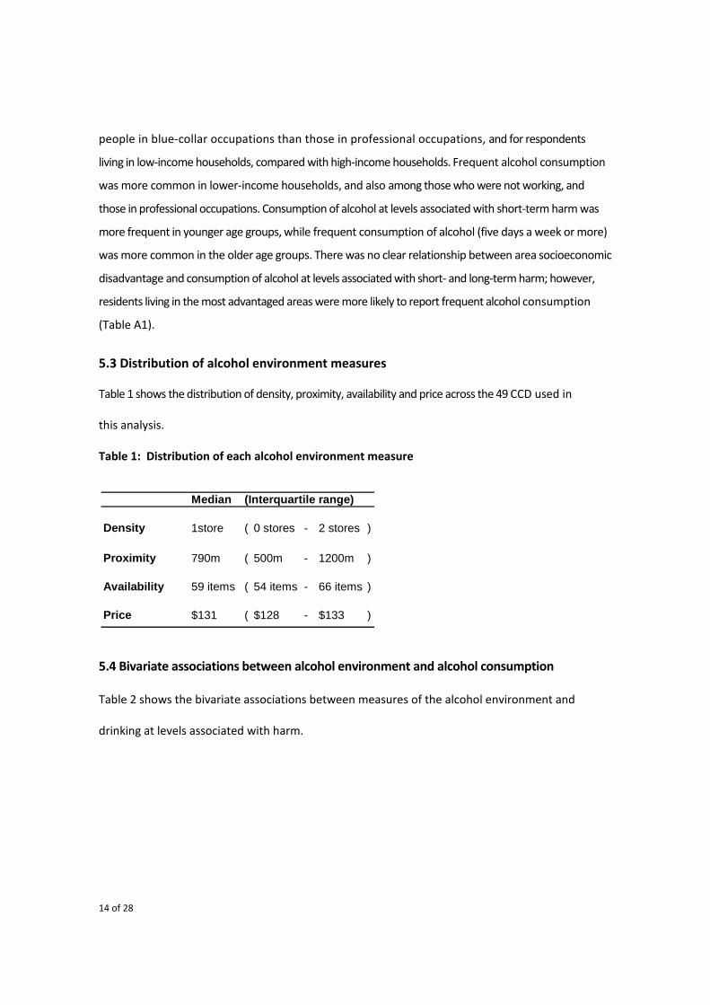
5.3 Distribution of alcohol environment measures

Table 1 shows the distribution of density, proximity, availability and price across the 49 CCD used in

this analysis.

Table 1: Distribution of each alcohol environment measure

5.4 Bivariate associations between alcohol environment and alcohol consumption

Table 2 shows the bivariate associations between measures of the alcohol environment and

drinking at levels associated with harm.

Median (Interquartile range)

Density 1store ( 0 stores - 2 stores )

Proximity 790m ( 500m - 1200m )

Availability 59 items ( 54 items - 66 items )

Price $131 ( $128 - $133 )

15 of 28

Table 2: Associations between alcohol consumption and alcohol environment measures

Descriptive analysis based on 25,690 observations (imputed data)

Variable Category (%) Frequent

Harm % (95% CI) Harm % (95% CI) Harm % (95% CI) Harm % (95% CI)

DensityNo stores ( 38 ) 12 ( 10 - 14 ) 29 ( 26 - 32 ) 5 ( 4 - 6 ) 16 ( 14 - 19 )1 ( 26 ) 13 ( 10 - 16 ) 28 ( 25 - 32 ) 4 ( 3 - 6 ) 21 ( 17 - 24 )2 ( 14 ) 12 ( 8 - 15 ) 28 ( 23 - 33 ) 6 ( 3 - 8 ) 19 ( 14 - 23 )3 to 4 ( 10 ) 18 ( 13 - 23 ) 36 ( 30 - 42 ) 9 ( 5 - 12 ) 21 ( 16 - 27 )5 to 7 ( 9 ) 15 ( 10 - 20 ) 37 ( 30 - 43 ) 6 ( 3 - 10 ) 20 ( 14 - 26 )8 + ( 4 ) 25 ( 16 - 34 ) 41 ( 31 - 52 ) 9 ( 3 - 15 ) 19 ( 11 - 28 )Trend P= P= P= P=

Proximity1.2km + ( 26 ) 12 ( 10 - 15 ) 30 ( 26 - 33 ) 4 ( 3 - 6 ) 16 ( 13 - 19 ) 0.8 to <1.2 km ( 23 ) 13 ( 10 - 16 ) 31 ( 27 - 35 ) 6 ( 4 - 8 ) 18 ( 14 - 21 ) 0.4 to <0.8 km ( 33 ) 13 ( 11 - 15 ) 28 ( 25 - 31 ) 6 ( 4 - 7 ) 21 ( 18 - 24 ) < 0.4 kms ( 17 ) 17 ( 14 - 21 ) 35 ( 30 - 40 ) 7 ( 4 - 10 ) 19 ( 15 - 23 )Trend P= P= P= P=

Availability< 40 items ( 13 ) 15 ( 11 - 19 ) 32 ( 27 - 38 ) 9 ( 6 - 12 ) 22 ( 17 - 27 )40 to 49 items ( 6 ) 9 ( 4 - 14 ) 25 ( 18 - 33 ) 2 ( 0 - 4 ) 11 ( 5 - 17 )50 to 59 items ( 33 ) 13 ( 10 - 15 ) 29 ( 25 - 32 ) 5 ( 4 - 7 ) 21 ( 17 - 24 )60+ items ( 48 ) 13 ( 11 - 15 ) 30 ( 28 - 33 ) 5 ( 4 - 6 ) 17 ( 15 - 20 )Trend P= P= P= P=

Price< $130 ( 30 ) 13 ( 10 - 15 ) 27 ( 24 - 31 ) 6 ( 4 - 7 ) 20 ( 17 - 24 )$130 to < $135 ( 59 ) 12 ( 10 - 14 ) 30 ( 28 - 33 ) 5 ( 4 - 6 ) 17 ( 15 - 19 )$135 to < $140 ( 5 ) 20 ( 12 - 28 ) 37 ( 27 - 47 ) 8 ( 3 - 14 ) 23 ( 14 - 32 )$140+ ( 6 ) 15 ( 9 - 21 ) 36 ( 27 - 44 ) 9 ( 4 - 14 ) 24 ( 16 - 31 )Trend P= P= P= P=

0.814 0.090 0.4520.906

Measure of Alcohol Consumption

0.264 0.555 0.107

0.006 0.004


Short-term harm (monthly)

Long-term harm

0.319 0.8440.1930.022

0.024 0.211

0.296

16 of 28

Density

As the number of alcohol outlets increased, the risk of consumption at levels associated with long‐term

harm and short‐term harm, weekly, and short‐term harm, monthly, increased (P for trend 0.024,

0.006 and 0.004, respectively) (Table 2).

Proximity

There were no statistically‐significant associations between proximity and drinking at levels associated

with harm but the highest levels of drinking for short‐term harm (both weekly and monthly) were

found in the respondents living closest to an outlet (Table 2).

Availability

There was no evidence to support an association between the availability of alcoholic beverages in

stores and drinking at levels associated with harm (Table 2).

Price

The prevalence of drinking at levels associated with short‐term harm, at least monthly, increased,

as the price of the basket of alcohol increased (P = 0.022) (Table 2).

5.5 Multilevel regression analyses

Density

The density of outlets was linearly associated with increased risk of all measures of harmful alcohol

consumption (Table 3). The risk of harmful consumption was highest when there were eight or

more outlets (short‐term harm, weekly: OR 2.36, 95 per cent CI: 1.12–4.54 and short‐term harm,

monthly: OR 1.80, 95 per cent CI: 1.07–3.04) (Table 3; Figures 2 and 3).

17 of 28

Table 3: Relationship between density of alcohol stores and alcohol consumption

Table 4: Relationship between proximity to nearest alcohol store and alcohol consumption

Variable Short Term (weekly) Short term (monthly) Long Term Frequent OR (95% CI) OR (95% CI) OR (95% CI) OR (95% CI)

Categorical MeasureNone 1.00 1.00 1.00 1.001 1.15 ( 0.79 - 1.66 ) 1.01 ( 0.77 - 1.32 ) 0.86 ( 0.51 - 1.45 ) 1.29 ( 0.95 - 1.76 )2 0.95 ( 0.60 - 1.50 ) 0.95 ( 0.68 - 1.33 ) 1.10 ( 0.60 - 2.01 ) 1.24 ( 0.84 - 1.81 )3 to 4 1.75 ( 1.12 - 2.76 ) 1.41 ( 0.99 - 2.00 ) 1.69 ( 0.95 - 3.01 ) 1.33 ( 0.88 - 1.99 )5 to 7 1.32 ( 0.79 - 2.21 ) 1.56 ( 1.07 - 2.28 ) 1.29 ( 0.65 - 2.57 ) 1.46 ( 0.94 - 2.28 )8 + 2.36 ( 1.22 - 4.54 ) 1.80 ( 1.07 - 3.04 ) 1.47 ( 0.62 - 3.46 ) 1.36 ( 0.71 - 2.62 )

Test for trendP Value 0.009 0.002 0.092 0.077

Type of Harm


Categorical Measure1.2+ kms 1.00 1.00 1.00 1.00 0.8 to <1.2 km 0.98 ( 0.65 - 1.48 ) 1.18 ( 0.86 - 1.63 ) 1.39 ( 0.80 - 2.44 ) 1.21 ( 0.83 - 1.77 ) 0.4 to <0.8 km 1.04 ( 0.70 - 1.57 ) 0.98 ( 0.73 - 1.33 ) 1.31 ( 0.77 - 2.25 ) 1.43 ( 1.03 - 2.00 ) < 0.4 kms 1.29 ( 0.81 - 2.05 ) 1.35 ( 0.95 - 1.91 ) 1.53 ( 0.84 - 2.81 ) 1.33 ( 0.87 - 2.02 )


Type of Harm

18 of 28

Figure 2: Odds of consumption at levels associated with short‐term harm (weekly) by number

of stores (within 1‐kilometre network distance) compared to no stores

Figure 3: Odds of consumption at levels associated with short‐term harm (monthly) by number

of stores (within 1‐kilometre network distance) compared to no stores

Proximity

We did not find evidence to support an association between proximity of alcohol outlets and

alcohol consumption at levels associated with short‐ or long‐term harm or frequency of consumption

when proximity was fitted as a continuous or categorical variable (Table 4).

0.00

0.50

1.00

1.50

2.00

2.50

3.00

3.50

4.00

4.50

5.00

None(reference)

1 2 3 to 4 5 to 7 8 +

Number of stores within 1km network distance

Odd

s ra

tio

Odds of Short TermHarm (weekly)

95% confidence interval

0.00

0.50

1.00

1.50

2.00

2.50

3.00

3.50

None(reference)

1 2 3 to 4 5 to 7 8 +

Number of stores within 1km network distance

Odd

s ra

tio Odds of Short TermHarm (monthly)


19 of 28

Table 5: Relationship between availability of items in nearest alcohol store and alcohol consumption

Table 6: Relationship between price of items in nearest alcohol store and type of harm


Categorical Measure< 40 items 1.00 1.00 1.00 1.0040 to 49 items 0.45 ( 0.19 - 0.99 ) 0.71 ( 0.40 - 1.26 ) 0.20 ( 0.04 - 0.88 ) 0.67 ( 0.32 - 1.39 )50 to 59 items 0.81 ( 0.51 - 1.27 ) 0.84 ( 0.59 - 1.19 ) 0.57 ( 0.32 - 1.00 ) 0.93 ( 0.63 - 1.38 )60+ items 0.75 ( 0.48 - 1.14 ) 0.88 ( 0.64 - 1.23 ) 0.55 ( 0.33 - 0.94 ) 0.79 ( 0.53 - 1.18 )


Type of Harm


Categorical Measure< $130 1.00 1.00 1.00 1.00$130 to < $135 0.89 ( 0.65 - 1.23 ) 1.08 ( 0.85 - 1.38 ) 0.82 ( 0.53 - 1.28 ) 0.83 ( 0.66 - 1.09 )$135 to < $140 1.55 ( 0.82 - 2.92 ) 1.40 ( 0.83 - 2.35 ) 1.22 ( 0.52 - 2.84 ) 1.40 ( 0.79 - 2.48 )$140+ 1.29 ( 0.68 - 2.44 ) 1.41 ( 0.87 - 2.28 ) 1.42 ( 0.66 - 3.07 ) 1.08 ( 0.63 - 1.85 )


Type of Harm

20 of 28

Availability

Although there was not a statistically‐significant association between availability of alcoholic

beverages and alcohol consumption at levels associated with harm, when availability was fitted as a

continuous variable, when availability was fitted as a categorical variable, we found some evidence to

suggest that access to a larger variety of beverages reduced consumption associated with long‐

term harm (Table 5; Figure 4).

Figure 4: Odds of consumption at levels associated with long‐term harm by availability of

items in nearest store, compared to ‘less than 40 items’

Price

The price of a basket of alcohol beverages was not associated with consumption of alcohol at

levels that increase risk of harm, when price was fitted as a continuous or categorical variable.

The significant trend found between price, fitted as categorical variable, and short‐term harm,

monthly, found in the bivariate analysis, did not remain when controlling for potential confounders

(Table 6).

0.00

0.20

0.40

0.60

0.80

1.00

1.20

< 40 items 40 - 49 items 50 - 59 items 60+ items

Number of items available in closest store

Odd

s ra

tio

Odds of Long TermHarm


21 of 28

6. Discussion

6.1 Discussion of findings

Density

Access to an increased number of alcohol outlets is associated with a higher risk of drinking at

levels associated with harm. We found evidence to suggest that the association between

outlet density and consuming alcohol at levels associated with short‐term harm might not be

strictly linear. When outlet density was fitted as a categorical variable, the increased risk of

drinking at levels associated with short‐term harm, at least weekly, was observed when there

were three to four, and eight or more outlets within a one‐kilometre network area. An

increased risk of drinking at levels associated with harm, at least monthly, was observed

when there were five or more outlets. We therefore find evidence to suggest that when the

number of outlets in an area of a one‐kilometre network distance is eight or more, the risk of

drinking at levels associated with short‐term harm (weekly and monthly) is increased.

Although the association between outlet density and both frequent consumption and

drinking at levels associated with long‐term harm were not statistically significant (P = 0.077

for frequent consumption, P = 0.092 for long‐term harm), the direction of the effects are

suggestive of a positive association. As consumption at levels associated with long‐term

harm was less common than drinking at levels associated with short‐term harm; this might

have reduced our power to detect a statistically‐significant effect. The lack of a

significant association between outlet density and increases in ‘average consumption’ has

also been reported by Connor et al. in a study conducted in New Zealand (Connor et al. 2010).

Proximity

Given that we found associations between outlet density and harmful alcohol consumption, the

lack of evidence to support an association between proximity and consumption is surprising.

The potential explanation for the lack of association between proximity and consumption

might be due to the limited range of values for proximity in our sample, with 75 per cent of

participants having an outlet within 1.2 kilometres of their home. This small exposure gradient

might have limited our power to detect an association between proximity and consumption.

However, our findings are consistent with other studies, whereby associations between outlet

density and consumption have been reported (Kypri et al. 2008; Livingston, Laslett & Dietze

2008; Schonlau et al. 2008), while no studies have found an association between proximity and

consumption (Pollack et al. 2005; Scribner, Cohen & Fisher 2000).

22 of 28

Availability

We found some limited evidence to suggest that access to a greater variety of alcoholic

beverages reduced the risk of drinking at levels associated with long‐term harm. Although this

result might seem counterintuitive, the larger variety of beverages provides consumers with

greater choice, and beverages with low alcohol content (e.g. light beers) might be more readily

available. Further study is needed to investigate this association.

Price

In our study, there was no evidence of an association between the price of a basket of

commonly‐available items and levels of alcohol consumption. This finding does not accord with

previous research, which has demonstrated that consumption is strongly related to price

(Wagenaar, Salois & Komro 2009). However, most other studies have been ecological, or if

based on individual outcome data, have used area‐level measure of alcohol access. In

addition, many of the individual‐level studies have been conducted on youth populations

that might be more sensitive to changes in price (Elder et al. 2010). We are unaware of any

studies other than ours that have investigated this using multilevel modelling and individual

measures of alcohol access.

One of the reasons we might have not found an association between price and consumption is

that there was very little variability in the price of beverages between stores. It may be that

consumption levels are affected by much larger fluctuations in price than we could test in this study.

6.2 Strengths and limitations

We discuss the strengths and limitations of this study, and summarise some of the complex

methodological issues.

Limitations

First, it is possible that respondents self‐selected into areas in such a way that people who are

at risk of drinking at levels associated with harm might have also lived in areas with a higher

density of outlets. This self‐selection could potentially result in overestimates of the

association between outlet density and consumption. However, people in higher socio‐

economic groups are more able to choose their place of residence, and we controlled for

three measures of individual and household socio‐economic position. Therefore, we believe it

is unlikely that self‐selection could account for the results. Second, we used a one‐kilometre

23 of 28

network distance, which is approximately equivalent to a 15‐minute walk or a five‐minute

car ride, and thus outlets at this distance would be highly accessible to people’s homes.

We fitted densities with higher buffer distances and found that they yielded similar but

slightly attenuated results. Third, this study is cross‐sectional, and thus we cannot

conclude the associations are causal, as businesses that sell alcohol might set up in areas

where there is already a high prevalence of people drinking at levels associated with harm.

Intervention studies are needed to test the impact of changes in the exposure to alcohol

outlets on changes in consumption. In addition, levels of alcohol consumption were self‐

reported, and it is likely that these were underestimated by respondents.

Strengths

The study has considerable strengths. First, our measures of access to alcohol outlets are more

sophisticated than those used previously. We measure density and proximity using road

network distance, calculated from respondents’ homes, while previous studies used measures derived

from administrative units or calculated using Eucidian distances. We also collected detailed information

on the variety of beverages in stores and their prices. To our knowledge, this detailed information has

not been collected previously in Australia. Second, we were able to control for a large number of

confounders, including individual and area‐level socioeconomic position and potential predictors of

self‐selection, thus minimising the possibility of residual confounding.

Summary of methodological issues

Some of the complex methodological difficulties are detailed in the Appendix. Briefly, these related to

missing data on key socioeconomic variables, and the fact that many stores only stocked a

limited range of beverages. This required us to conduct multiple imputation to obtain values for

missing data items. Additionally, many of the CCD were very close to each other, and it is possible that

measures of alcohol access and consumption might have been correlated across CDD. However,

we conducted sensitivity analyses to address this problem, and concluded that it did not alter our

estimates. Finally, it is possible that unmeasured characteristics of areas might confound the

associations between alcohol access and consumption.

24 of 28

7. Recommendations

Based on our findings, we suggest that policy interventions that restrict the number of outlets

selling liquor for off‐premise consumption in areas could reduce consumption at levels

associated with harm. We do not provide evidence to support policies that restrict the

number of beverages that stores stock. In addition, we do not find evidence to support

increasing the price if alcohol to reduce consumption; however, we believe that our study

might not have been able to detect an association, because there was so little variation in the

prices of beverages between stores.

We recommend that future research, possibly supported by VicHealth, assess the impact of

policy interventions, such as limiting the number of alcohol licenses in areas or monitoring the

impact of increases in the price of beverages. Furthermore, we did not assess whether

access to outlets for on‐premise consumption influenced the levels of consumption, and this

is likely to be a fruitful area of future research.

In sum, we recommend that:

• policy makers and practitioners consider implementing strategies to reduce the

number of stores that sell alcohol for off‐premise consumption

• rigorous evaluation of policy initiatives to restrict access to stores or to increase

the price of beverages is funded

• research that examines the impact of access to premises that sell alcohol

consumption on site be funded.

25 of 28

8. References

Anderson, P & Baumberg, B 2006, Alcohol in Europe: a public health perspective. A report for the European Commission, Institute of Alcohol Studies, London.

Australian Bureau of Statistics 2006, Census dictionary, 2006 (reissue), ABS, Canberra, <http://www.abs.gov.au/ausstats/[email protected]/Latestproducts/2901.0Contents12006%20(Reissue)?opendocument&tabname=Summary&prodno=2901.0&issue=2006%20(Reissue)&num=&view=>.

Australian Electoral Commission 2005, Measuring the accuracy of the electoral rolls and testing the effectiveness of the continuous roll update, Australian Electoral Commission, Canberra.

Australian Institute of Health and Welfare 2002, National Drug Strategy Household Survey: first results, AIHW, Canberra.

—— 2007, Statistics on drug use in Australia 2006, AIHW, Canberra, DOI cat no. PHE 80.

Chen, M, Grube, J & Gruenewald, P 2010, 'Community alcohol outlet density and underage drinking', Addiction, vol. 105, pp. 270‐8.

Chikritzhs, T, Catalano, P, Pascal, R & Hendrickson, N 2007, Predicting alcohol‐related harms from licensed outlet density: a feasibility study, National Drug Research Institute & Western Australian Drug and Alcohol Office, Perth.

Connor, JL, Kypri, K, Bell, ML & Cousins, K 2010, 'Alcohol outlet density, levels of drinking and alcohol‐related harm in New Zealand: a national study', Journal of Epidemiology and Community Health, vol. 65, pp. 841‐6.

Dillman, D 2000, Mail and internet surveys: the tailored design method, 2nd edn, John Willey, New York.

Elder, RW, Lawrence, B, Ferguson, A, Naimi, TS, Brewer, RD, Chattopadhyay, SK, Toomey, TL & Fielding, JE 2010, 'The effectiveness of tax policy interventions for reducing excessive alcohol consumption and related harms', American Journal of Preventative Medicine, vol. 38, no. 2, pp. 217‐29.

Gruenewald, P, Johnson, F & Treno, A 2002, 'Outlets, drinking and driving: a multilevel analysis', Journal of Studies on Alcohol, vol. 63, pp. 460‐8.

Hewko, J, Smoyer‐Tomic, KE & Hodgson, MJ 2002, 'Measuring neighbourhood spatial accessibility to urban amenities: does aggregation error matter?', Environment and Planning, vol. 34, no. 7, pp. 1185‐206.

Hibell, B, Andersson, B, Bjarnason, T, Ahlstrom, S, Balakireva, O, Kokkevi, A & Morgan, M 2004, The ESPAD report 2003: alcohol and other drug use among students in 35 European countries, Swedish Council for Information on Alcohol and Other Drugs, Stockholm.

Kavanagh, A, Thornton, L, Tattam, A, Thomas, L, Jolley, D & Turrell, G 2007, Place does matter for your health: a report of the Victorian Lifestyle and Neighbourhood Environment Study, University of Melbourne, Melbourne.

Klebanoff, MA & Cole, SR 2008, 'Use of multiple imputation in the epidemiological literature', American Journal of Epidemiology, vol. 168, no. 4, pp. 355‐7.

Kypri, K, Bell, M, Hay, G & Baxter, J 2008, 'Alcohol outlet density and university student drinking: a national study', Addiction, vol. 103, no. 7, pp. 1131‐8.

Liquor Control Advisory Council 2007, Report on the appropriateness of the regulatory regime for the sale of packaged liquor in Victoria: issues paper, Consumer Affairs Victoria, Melbourne, <http://www.consumer.vic.gov.au/CA256902000FE154/Lookup/CAV_Publications_Liquor_Licensing_2/$file/liquor_misc_packaged_liquor_issues_paper.doc>.

Liquor Licensing Victoria 2002, Licence details as at 8 December, 2002, State Government of Victoria.

26 of 28

Livingston, M, Laslett, A‐M & Dietze, P 2008, 'Individual and community correlates of young people's high‐risk drinking in Victoria, Australia', Drug and Alcohol Dependence, vol. 98, no. 3, pp. 241‐8.

Matisziw, TC, Grubesic, TH & Wei, H 2008, 'Downscaling spatial structure for the analysis of epidemiological data', Computers, Environment and Urban Systems, vol. 32, no. 1, pp. 81‐93.

Menvielle, G, Kunst, A, Stirbu, I, Borrell, C, Bopp, M, Regidor, E, Strand, BH, Deboosere, P, Lundberg, O, Leclerc, A, Costa, G, Chastang, J‐F, Esnaola, S, Martikainen, P & Mackenbach, J 2007, 'Socioeconomic inequalities in alcohol related cancer mortality among men: to what extent do they differ between Western European populations?', International Journal of Cancer, vol. 121, no. 3, pp. 649‐55.

National Alcohol Strategy 2006‐2011, 2006, Ministerial Council on Drug Strategy.

National Health and Medical Research Council 2001, Australian alcohol guidelines: health risks and benefits, Commonwealth of Australia, Canberra. <http://www.nhmrc.gov.au/publications/subjects/substance.htm>.

—— 2007, Australian alcohol guidelines for low‐risk drinking: draft for public consultation, Australian Government, Canberra.

National Preventative Health Taskforce 2008, Technical Report No 3: Preventing alcohol‐related harm in Australia: a window of opportunity, Australian Government, Canberra.

Nelson, J 2008, 'How similar are youth and adult alcohol behaviours? Panel results for excise taxes and outlet density', Atlantic Economic Journal, vol. 36, no. 1, pp. 89‐104.

Pollack, C, Cubbin, C, Ahn, D & Winkleby, M 2005, 'Neighbourhood deprivation and alcohol consumption: does the availability of alcohol play a role?', International Journal of Epidemiology, vol. 34, no. 4, pp. 772‐80.

Schonlau, M, Scribner, R, Farley, T, Theall, K, Bluthenthal, R, Scott, M & Cohen, D 2008, 'Alcohol outlet density and alcohol consumption in Los Angeles county and southern Louisiana', Geospatial Health, vol. 3, no. 1, pp. 91‐101.

Scribner, R, Cohen, D & Fisher, W 2000, 'Evidence of a structural effect for alcohol outlet density: a multilevel analysis', Alcoholism: Clinical and Experimental Research, vol. 24, no. 2, pp. 188‐95.

The Honourable Nicola Roxon MP Alcopops tax loophole finally closed, Department of Health and Ageing: Canberra. 13 August 2009, <http://www.health.gov.au/internet/ministers/publishing.nsf/Content/mr‐yr09‐nr‐nr120.htm, accessed 1 March 2011>.

Wagenaar, AC, Salois, MJ & Komro, KA 2009, 'Effects of beverage alcohol price and tax levels on drinking: a meta‐analysis of 1003 estimates from 112 studies', Addiction, vol. 104, no. 2, pp. 179‐90.

World Health Organization 2007, WHO Expert Committee on Problems Related to Alcohol Consumption: second report, WHO, Geneva.

27 of 28

9. Appendix

9.1 Alcohol consumption and demographics

Table A1: Associations between alcohol consumption and demographics (descriptive analysis based on 25,690 observations (imputed data))

Variable Category ( % ) Frequent

Harm % (95 % C I) Harm % (95 % C I) Harm % (95 % C I) Harm % (95 % C I)SexMale ( 44 ) 19 ( 17 - 22 ) 38 ( 35 - 41 ) 6 ( 5 - 8 ) 24 ( 21 - 27 )Female ( 56 ) 9 ( 7 - 11 ) 25 ( 23 - 27 ) 5 ( 4 - 6 ) 14 ( 12 - 17 )χ2 P= <0.001 P= <0.001 P= P= <0.001Aust BornNo ( 29 ) 6 ( 4 - 8 ) 16 ( 13 - 19 ) 3 ( 1 - 4 ) 17 ( 14 - 21 )Yes ( 71 ) 17 ( 15 - 18 ) 36 ( 34 - 39 ) 7 ( 6 - 8 ) 19 ( 17 - 21 )χ2 P= P= <0.001 P= P=Household TypeOne adult ( 18 ) 18 ( 14 - 22 ) 32 ( 28 - 37 ) 7 ( 4 - 9 ) 18 ( 14 - 22 )One adult, children ( 6 ) 14 ( 8 - 20 ) 27 ( 29 - 34 ) 4 ( 0 - 7 ) 14 ( 8 - 20 )2 or more adults ( 41 ) 16 ( 13 - 18 ) 36 ( 33 - 39 ) 7 ( 5 - 8 ) 20 ( 18 - 23 )2 or more adults, children ( 35 ) 9 ( 7 - 11 ) 23 ( 20 - 26 ) 4 ( 3 - 5 ) 18 ( 15 - 21 )χ2 P= <0.001 P= P= P=EducationBachelor or higher ( 32 ) 11 ( 9 - 13 ) 29 ( 26 - 32 ) 6 ( 4 - 8 ) 21 ( 18 - 24 )Diploma ( 12 ) 8 ( 5 - 12 ) 26 ( 20 - 31 ) 3 ( 1 - 5 ) 19 ( 14 - 24 )Vocational ( 20 ) 18 ( 14 - 22 ) 35 ( 31 - 40 ) 6 ( 4 - 8 ) 21 ( 17 - 25 )No post school ( 37 ) 15 ( 13 - 17 ) 31 ( 27 - 34 ) 6 ( 4 - 8 ) 16 ( 13 - 18 )Trend P= P= P= P=Occupation Professional ( 36 ) 12 ( 10 - 14 ) 34 ( 30 - 37 ) 5 ( 4 - 7 ) 21 ( 18 - 24 )White Collar ( 16 ) 15 ( 11 - 18 ) 35 ( 30 - 40 ) 6 ( 3 - 8 ) 12 ( 8 - 15 )Blue Collar ( 12 ) 25 ( 20 - 30 ) 42 ( 36 - 48 ) 6 ( 3 - 9 ) 15 ( 10 - 19 )Not working ( 35 ) 11 ( 9 - 13 ) 21 ( 18 - 24 ) 6 ( 4 - 8 ) 21 ( 18 - 24 )χ2 P= P= P= P=Income (per annum)$20,799 or less ( 30 ) 14 ( 11 - 17 ) 38 ( 34 - 42 ) 6 ( 4 - 8 ) 23 ( 20 - 27 )$20,800 to $36,399 ( 20 ) 13 ( 10 - 17 ) 31 ( 26 - 36 ) 7 ( 4 - 9 ) 18 ( 14 - 22 )$36,400 to $51,999 ( 17 ) 13 ( 9 - 16 ) 29 ( 24 - 34 ) 5 ( 2 - 7 ) 17 ( 12 - 21 )$52,000 to $77,999 ( 17 ) 14 ( 11 - 18 ) 25 ( 21 - 30 ) 5 ( 2 - 7 ) 15 ( 12 - 19 )$78,000 or more ( 17 ) 13 ( 10 - 17 ) 23 ( 18 - 28 ) 5 ( 3 - 7 ) 16 ( 12 - 20 )Trend P= P= P= P=Age18 to 24 ( 8 ) 23 ( 17 - 29 ) 55 ( 48 - 62 ) 8 ( 4 - # ) 3 ( 1 - 6 )25 to 34 ( 18 ) 19 ( 15 - 22 ) 42 ( 37 - 47 ) 7 ( 4 - 9 ) 8 ( 5 - 10 )35 to 44 ( 21 ) 13 ( 10 - 16 ) 32 ( 28 - 36 ) 4 ( 2 - 6 ) 14 ( 11 - 17 )45 to 54 ( 21 ) 12 ( 9 - 14 ) 26 ( 22 - 30 ) 5 ( 3 - 7 ) 23 ( 19 - 26 )55 to 64 ( 17 ) 11 ( 8 - 14 ) 24 ( 20 - 28 ) 6 ( 3 - 8 ) 28 ( 23 - 32 )65+ ( 15 ) 10 ( 6 - 13 ) 15 ( 11 - 19 ) 5 ( 3 - 8 ) 30 ( 25 - 35 )Trend P= P= P= P=StrataMost advantaged ( 36 ) 11 ( 9 - 13 ) 29 ( 26 - 32 ) 5 ( 4 - 7 ) 24 ( 21 - 27 )Middle ( 33 ) 15 ( 12 - 17 ) 33 ( 30 - 36 ) 7 ( 5 - 8 ) 17 ( 14 - 19 )Least advantaged ( 31 ) 15 ( 12 - 18 ) 29 ( 25 - 32 ) 5 ( 3 - 7 ) 15 ( 12 - 18 )Trend P= P= P= P= <0.0010.9540.700

0.409

<0.001<0.001 0.187

0.090

<0.001

<0.001 <0.001

0.612 <0.001

Measure of Alcohol Consumption

<0.001<0.001

0.001

0.001

<0.001<0.001


Short-term harm (monthly) Long-term harm

<0.001

0.002 0.580 0.1240.124

<0.001

0.179 0.012

28 of 28

9.2 Methodological issues

Multiple imputation of individual variables

Data were missing on a number of key variables, including income (35 per cent missing).

Complete data on all variables were available for 61 per cent of the sample. Rather than

analysing complete cases only, potentially biasing estimates, missing data were imputed

under a missing‐at–random, assumption where missing values were modelled as a function of

observed variables (Klebanoff & Cole 2008). Twenty datasets with imputed values for missing

items on each variable were estimated using the imputation by chained equations (ICE) command

in Stata 11.1. Analysis was undertaken in Stata 11.1 using the GLLAMM function, prefixed by

the user‐written ‘mim’ command (created by JC Galati, P Royston and JB Carlin), which allowed

for analysis to be undertaken across multiple datasets.

Multiple imputations of price of basket of alcohol in stores

Prices for missing items were also imputed, as described earlier. We might investigate multi‐item

response methods to assign values for stores in future analyses. However, further discussion

of this method is beyond the scope of this report.

Spatial autocorrelation

Many of the CCD were close geographically, so that in some situations, the individual

network buffers used to measure access overlapped for individuals in nearby CCD. This raises

the possibility of spatial autocorrelation that might not be accounted for in our current modelling

approach. We identified where overlap was possible finding 10 clusters of between two and six

CCD; however, models fitted with these CCD clusters as a random effect produced almost

identical results.

Residual confounding by area (fixed effects)

Finally, there is potential for residual confounding due to unmeasured area‐level

characteristics. To verify our findings, we ran models with CCD fitted as fixed effects. The

estimates obtained from these models were closer to the null, than for the random‐effects

models, but the direction of the effect remained the same (data not shown). Fixed‐effects

models will eliminate confounding, due to area effects, but reduces power, and might also result

in over adjustment for area‐level mediators of the associations between alcohol density and

proximity and risk of alcohol‐related harm. Thus, the true estimate is likely to lie somewhere

between the random‐ and fixed‐effects models.

Victorian Health Promotion Foundation PO Box 154 Carlton South, VIC 3053 Australia T +61 3 9667 1333 F +61 3 9667 1375 [email protected]

December 2011

accessibility to alcohol outlets and alcohol consumption

Documents