access to thesis
TRANSCRIPT

Access To Thesis.
This thesis is protected by the Copyright, Designs and Patents Act 1988. No reproduction is permitted without consent of the author. It is also protected by the Creative Commons
Licence allowing Attributions-Non-commercial-No derivatives.
• Aboundcopyofeverythesiswhichisacceptedasworthyforahigherdegree,mustbedepositedintheUniversityofSheffieldLibrary,whereitwillbemadeavailableforborrowingorconsultationinaccordancewithUniversityRegulations.
• Allstudentsregisteringfrom2008–09onwardsarealsorequiredtosubmitanelectroniccopyoftheirfinal,approvedthesis.Studentswhoregisteredpriorto2008–09mayalsosubmitelectronically,butthisisnotrequired.
Author:........................................................................................................................................................................... Dept:.................................................................................................................................................................
ThesisTitle:........................................................................................................................................................................................................................... RegistrationNo:..............................................................
For completion by all students:Submitinprintformonly(fordepositintheUniversityLibrary): n
SubmitinprintformandalsouploadtotheWhite Rose eTheses Online server: Infull n
EditedeThesis n
Please indicate if there are any embargo restrictions on this thesis. Please note that if no boxes are ticked, you will have consented to your thesis being made available without any restrictions.Embargodetails:(completeonlyifrequestingan Embargorequired? Lengthofembargoembargotoeitheryourprintand/oreThesis) (inyears)
PrintThesis Yesn Non _____
eThesis Yesn Non _____
Supervisor:I,thesupervisor,agreetothenamedthesisbeingmadeavailableundertheconditionsspecifiedabove.Name:………………………………………………………………………........................................................................... Dept:...............................................................................................................................................................
Signed:……………………………………………………………………………................................................................. Date:.................................................................................................................................................................
Student: I,theauthor,agreetothenamedthesisbeingmadeavailableundertheconditionsspecifiedabove.
IgivepermissiontotheUniversityofSheffieldtoreproducetheprintthesisinwholeorinpartinordertosupplysinglecopiesforthepurposeofresearchorprivatestudyforanon-commercialpurpose.
Iconfirmthatthisthesisismyownwork,andwherematerialsownedbyathirdpartyhavebeenusedcopyrightclearancehasbeenobtained.IamawareoftheUniversity’sGuidance on the Use of Unfair Means (www.sheffield.ac.uk/lets/design/unfair)
I confirm that all copiesof the thesis submitted to theUniversity (includingelectroniccopiesonCD/DVD)are identical incontent.
Name:………………………………………………………………………........................................................................... Dept:...............................................................................................................................................................
Signed:……………………………………………………………………………................................................................ Date:................................................................................................................................................................
For completion by students also submitting an electronic thesis (eThesis):I,theauthor,agreethattheUniversityofSheffield’seThesisrepository(currentlyWREO)willmakemyeThesisavailableovertheinternetviaanentirelynon-exclusiveagreementandthat,withoutchangingcontent,WREOmayconvertmythesistoanymediumorformatforthepurposeoffuturepreservationandaccessibility.
I,theauthor,agreethatthemetadatarelatingtotheeThesiswillnormallyappearonboththeUniversity’seThesisserverandtheBritishLibrary’sEThOSservice,evenifthethesisissubjecttoanembargo.IagreethatacopyoftheeThesismaybesuppliedtotheBritishLibrary.
Iconfirmthattheuploadisidenticaltothefinal,examinedandawardedversionofthethesisassubmittedinprinttotheUniversityfordepositintheLibrary(unlesseditedasindicatedabove).
Name:………………………………………………………………………........................................................................... Dept:.................................................................................................................................................................
Signed:……………………………………………………………………………................................................................ Date:................................................................................................................................................................
THIS SHEET MUST BE BOUND IN THE FRONT OF THE PRINTED THESIS BEFORE IT IS SUBMITTED

The Aerodynamics and Performance of Small Scale Wind Turbine Starting
A Dissertation Submitted for the Degree of Doctor of Philosophy
by
Dorit Sobotta
The University of Sheffield Department of Mechanical Engineering
October 2015

ABSTRACT
Small scale horizontal axis wind turbines (HAWTs) are becoming increasingly popular yet they have received much less research attention than their large scale counter parts. Unlike large scale rotors they solely rely on their aerodynamic torque for accelerating the blade from rest to full operational speed while being subjected to a number of torque reducing issues that large turbines do not experience.
In this study, Computational Fluid Dynamics (CFD) has been utilised to simulate turbine starting sequences. A newly developed method which uses CFD to model a fully transient turbine start-up has been evaluated. The chosen approach overcomes the assumptions of, currently employed, semi-empirical quasi-steady start-up methods. It has been shown that the quasi-steady approach is of acceptable accuracy in predicting starting sequences when compared to the fully transient method.
New techniques have been developed to investigate the flow features and local blade torque characteristics which have subsequently been quantified with respect to their relevance on turbine starting. The level of detail of the present study goes far beyond that of existing experimental or computational literature on turbine starting.
Following studies systematically investigated the effect of turbine scale and rotor geometry over a range of wind speeds using the National Renewable Energy Laboratory (NREL) Phase VI rotor as reference turbine. This analysis is the first of its kind which address the individual effect of blade pitch and thickness as well as their interdependence on the rotors performance at different operational Reynolds numbers. As a result of these studies, it has been shown, that the annual energy yield of turbines which frequently restart due to a turbulent flow environment, can be improved by increasing blade pitch and reducing blade thickness. It has been demonstrated that rotors with a small diameter are more resistant to energy yield reductions caused by gusty environments than larger rotors.
ii

DECLARATION
Described in this dissertation is work performed in the Department of Mechanical Engineering, the University of Sheffield between December 2009 and October 2015. I hereby declare that no part of this work has been submitted as an exercise for a degree at this or any other university. This dissertation is entirely the result of my own work and includes nothing which is the outcome of collaboration, except when stated otherwise. This dissertation contains 127 figures and approximately 66,000 words.
Dorit Sobotta
iii

ACKNOWLEDGEMENTS
I wish to thank my supervisors, Dr. Robert Howell at the University of Sheffield, UK and Dr. Lou Jing at the Institute of High Performance Computing, Singapore for their guidance, valuable advice and encouragement throughout the years of my Ph.D. Their expertise and mentoring has helped me to develop the skills required to critically plan, conduct and evaluate my own research. It has been a truly interesting experience to get an insight into different working environments and cultures, other than the one of my home country, Germany.
My gratitude also goes towards some of the current and past members of my research group, Jonny, Oke, Jon and Louis. The numerous chats we had in the office and in the lab provided constructive comments and feedback. They also lightened the spirit when I was facing seemingly insurmountable hurdles during my research.
Finally, I would like to thank my friends and family who have given me the kind of support needed to finish such a big research task. Throughout my stay in UK and Singapore I have met many new people from different countries, cultures and religious backgrounds who have made my Ph.D. an unforgettable experience.
iv

NOMENCLATURE
Symbols Ai area of cell i [m] c chord [m] cL, cD, cM lift, drag and moment coefficient [-] cf skin friction coefficient [-] cP power coefficient [-] cpr pressure coefficient [-] cT torque coefficient [-] 𝑐𝑐𝑇𝑇(𝑟𝑟𝑛𝑛) torque coefficient of the nth radial blade section [-]
𝑐𝑐𝑇𝑇 �𝑟𝑟𝑛𝑛𝑅𝑅� normalised torque coefficient of the nth radial blade section [-]
dt time step size [s] Ea actual energy over 10min interval [J] Ep potential energy generated during turbine starting [J] EF Energy Factor [-] I inertia [kg m2] k turbulent kinetic energy [m2/s2] N number of turbine blades [-] P power [W] P pressure [Pa] PS static pressure [Pa] r local radius [m] R blade radius [m] Re Reynolds number [-] s scale parameter for Rayleigh probability density function [-] tb blade thickness [m] T torque [Nm] T time [s] TG duration of a gust [s] TS time required for turbine starting [s] Taero aerodynamic torque [Nm] TA torque per unit area [Nm/m2] Ti torque over cell i [Nm] Tp pressure torque [Nm] Tres resistive torque [Nm] TN normalised torque [-] Tnet net torque [Nm] Tvis viscous torque [Nm] vrel relative wind speed [m/s] vrot rotational velocity component [m/s]
v

vin cut in wind speed of turbine [m/s] vout cut out wind speed of turbine below which negative torque is generated [m/s] vw wind speed [m/s] Y+ non-dimensional first cell height of wall adjacent cells [-] α angle of attack [°] αBlade angle of attack along the entire blade [°] αTip angle of attack at the blade tip [°] βpitch pitch angle [°] βtwist twist angle [°] ε dissipation rate [m2/s3] λ tip speed ratio [-] λα tip speed ratio when preserving α of differently pitched blades [-] λRe tip speed ratio when preserving Re of differently pitched blades [-] μ viscosity [Pas] μT eddy viscosity [Pas] ρ density [kg/m3] ω specific dissipation rate [1/s] ω rotational speed [rad/s] ω0 initial rotational speed [rad/s] ωN rotational speed at current time step [rad/s] ωN+1 rotational speed at next time step [rad/s]
Abbreviations AC Alternating Current AD Anno Domini AEY Annual Energy Yield BC Boundary Condition BEM Blade Element Momentum BL Boundary Layer CFD Computational Fluid Dynamics DC Direct Current EWT Enhanced Wall Treatment EY Energy Yield FAST Comprehensive code: Fatigue, Aerodynamics, Structures and Turbulence HAWT Horizontal Axis Wind Turbine HPC High Performance Computing IEC International Electrotechnical Commission KARI Korea Aerospace Research Institute LE Leading Edge LEV Leading Edge Vortex MRF Moving Reference Frame NACA National Advisory Committee for Aeronautics
vi

NREL National Renewable Energy Laboratory PIV Particle Image Velocimetry PM Permanent Magnet PS Pressure Surface P-V Pressure-Velocity R&D Research and Development RANS Reynolds Averaged Navier-Stokes RNG ReNormalization Group S-A Spalart-Allmaras SS Suction Surface SST Shear Stress Transport SWF Standard Wall Function TE Trailing Edge TEV Trailing Edge Vortex TU Model Turbulence Model TUI Text User Input UDF User Defined Function V&V Validation and Verification WT Wind Turbine WTRef Reference Wind Turbine (tb = 0.21c, βPitch = 0°) WTP Pitched Wind Turbine (tb = 0.21c, βPitch = 10°) WTT Thin-Bladed Wind Turbine (tb = 0.15c, βPitch = 0°) WTP-T Pitched and Thin-Bladed Wind Turbine (tb = 0.15c, βPitch = 10°) k-ε turbulence model family, variants investigated: Standard, RNG and Realizable k-ω turbulence model family, variants investigated: Standard and SST
vii

CONTENTS
ABSTRACT II
DECLARATION III
ACKNOWLEDGEMENTS IV
NOMENCLATURE V
CONTENTS VIII
1. INTRODUCTION 1
1.1 A Brief History of Converting Wind to Energy on a Small Scale 1
1.2 Modern Small Scale Wind Turbines 3
1.3 Increasing Underachievement with Decreasing Radius 5
1.4 Motivation to Investigate Wind Turbine Starting 8 1.4.1 Improving the Understanding of Turbine Starting 9 1.4.2 Potential to Increase Annual Energy Yield 10
1.5 Aims and Objectives 12
1.6 Thesis Outline 13
2. WIND TURBINE THEORY AND LITERATURE 15
2.1 Introduction 15
2.2 Fundamental Aerodynamics 16 2.2.1 Aerofoil Flow Physics 16 2.2.2 Wind Turbine Flow Physics 18
2.3 Relevant Structural Properties of Wind Turbines 24 2.3.1 Turbine Inertia 24 2.3.2 Generator 25
2.4 Starting of Small Scale HAWTs 25 2.4.1 Analysing Typical Starting Sequences 27 2.4.2 Effect of Turbine Scale 33 2.4.3 Effect of Blade Pitching 37 2.4.4 Effect of Blade Profile 39 2.4.5 Improvement Potential 42
viii

2.5 Quasi-Steady Start-Up Models 44 2.5.1 Quasi-Steady Assumption 45 2.5.2 Blade Element Theories 45
2.6 Computational Fluid Dynamics Review 47 2.6.1 Turbulence Models 47 2.6.2 Solver 53 2.6.3 Spatial Discretisation 55
2.7 Description of Reference Turbine Used in this Thesis 57
3. COMPUTATIONAL METHODS 59
3.1 Introduction 59
3.2 Aerofoil Simulation Validation and Verification 60 3.2.1 Spatial Discretisation 60 3.2.2 Aerodynamic Coefficients 61 3.2.3 Flow Field 68
3.3 Wind Turbine Simulation Validation and Verification 72 3.3.1 Spatial Discretisation 73 3.3.2 Constant Rotational Speed Performance 75 3.3.3 Transient Turbine Start-Up 84 3.3.4 Start-Up Methodology 87
3.4 Summary 92
4. AERODYNAMIC PERFORMANCE OF THE REFERENCE BLADE 94
4.1 Introduction 94
4.2 Reference Flow Condition 95 4.2.1 Power and Torque 95 4.2.2 Flow Field 101
4.3 Reynolds Number Effect 106 4.3.1 Turbine Scale 106 4.3.2 Varying Wind Speed at Different Turbine Scales 111
4.4 Summary 114
5. AERODYNAMIC ANALYSIS OF BLADE PARAMETERS 116
5.1 Introduction 116
5.2 Role of Blade Pitch 117 5.2.1 Torque Performance at Reference Condition 118 5.2.2 Flow Field at Reference Conditions 123 5.2.3 Effect of Reynolds Number 130
5.3 Role of Blade Thickness 133 5.3.1 Torque Performance at Reference Conditions 133 5.3.2 Flow Field at Reference Conditions 138
ix

5.3.3 Effect of Reynolds Number 140
5.4 Combined Effect of Pitch and Thickness 143 5.4.1 Torque Performance at Reference Conditions 143 5.4.2 Flow Field at Reference Conditions 149 5.4.3 Effect of Reynolds Number 152
5.5 Applicability of Lower Order BEM Methods 154 5.5.1 Comparison between BEM Assumptions and CFD Results 155 5.5.2 BEM Input Data 155
5.6 Summary 156
6. WIND TURBINE STARTING 159
6.1 Introduction 159
6.2 Typical Starting Sequences 160 6.2.1 Reference Blade 161 6.2.2 Effect of Blade Geometry 163
6.3 Turbine Starting on Energy Yield 167 6.3.1 Starting Time Analysis 168 6.3.2 Energy Output 169 6.3.3 Annual Energy Yield 172
6.4 Summary 175
7. CONCLUSIONS AND RECOMMENDATIONS 178
7.1 Introduction 178
7.2 Modelling of Turbine Starting 179
7.3 Improving the Understanding of Turbine Starting 180 7.3.1 Generic Turbine Starting Conclusions 180 7.3.2 Conclusions of Geometry Influence on Turbine Starting 181
7.4 Increasing Annual Energy Yield 183
7.5 Recommendations 184 7.5.1 Start-Up Modelling 184 7.5.2 Turbine Configurations 186
8. REFERENCES 188
9. APPENDIX 195
9.1 HAWT Meshing 195 9.1.1 Matlab 195 9.1.2 Gridgen 196
9.2 Useful Fluent TUI Commands 197
x

9.3 Turbulence Model Analysis & Mesh Analysis 197 9.3.1 Solver Study: Standard k-ɛ Model, EWT 199 9.3.2 Solver Study: k-ɛ RNG Model, EWT 200 9.3.3 S-A Model 201 9.3.4 k-ɛ Model, SWF 202 9.3.5 k-ɛ Model, EWT 203 9.3.6 k-ω Model 204
9.4 Start-Up UDF 205
xi

1. INTRODUCTION
1.1 A Brief History of Converting Wind to Energy on a Small Scale
The use of windmills to convert wind into energy has a long tradition. The first properly documented windmill appears in 644 AD at the Persian-Afghanistan border [1]. These early windmills were of simple nature and used the aerodynamic drag to rotate around a horizontal axis to perform tasks such as pumping water or grinding grain [2]. It wasn’t until the 12th century that lift type windmills that rotate around a horizontal axis appear in literature [3]. The American pioneer Brush laid a mile stone by constructing the first horizontal axis wind turbine that produced electricity in his back yard in the winter of 1887-88. His Wind Turbine (WT) had a radius of 8.5m and produced 12kW of DC power at its peak performance.
In the 19th century many attempts had been made worldwide at building small wind turbines as part of electrification programs for remote farms that otherwise had no access to electricity. A significant number of those attempts failed however due to turbine failure, blade damage, diminishing interest in wind energy and too complex construction of the blades or the blade-rotor joints [1]. Two highly successful small scale wind turbine models however were the turbines designed by the brothers Marcellus and Joseph Jacobs in 1922 and the Wincharger model which was designed by John and Gerhard Albers 5 years later. Tens of thousands of each unit have been sold worldwide with the production of the Wincharger peaking at 2,000 units a day. The success of the Jacobs turbine was built on its long life time of up to 22 years and its low maintenance requirement while the Wincharger was scoring with its low cost [1, 4, 5]; two factors which still heavily influence today’s small scale wind turbine market.

1. INTRODUCTION
Figure 1.1, Campaigns of The Jacobs Turbine [1] and the Wincharger [4]
The original Jacobs turbine had a radius of 2m and different models of the 3-bladed turbine produced a DC power output in the range of 1.8 to 3kW. The smaller Wincharger only had 2 blades and produced approximately 0.5kW at 1.2m radius and 1.2kW at 1.7m. An aerodynamic efficiency of just above 0.2 for small scale wind turbines was common at that time.
The boom of small scale wind turbines however came to an end in the 1950’s when the electricity provided by power lines became cheaper than wind energy. Difficulties in tying turbines of a variable voltage and frequency output to an AC grid of constant voltage and frequency, made room for charcoal and oil to become the primary source of energy. It wasn’t until the power generation through oil, charcoal or uranium faced increasing opposition, that wind energy was rediscovered as one of the alternative energy sources [1, 5]. An early solution of synchronising the power output frequency of a turbine with that of the grid had been to run the turbine at a fixed rotational speed which resulted in a reduced turbine performance. It was only in the 1970’s that engineers developed different methods to convert variable voltage and frequency outputs to constant voltage and frequency outputs. This allowed the construction of variable speed turbines which increased the power output as it allows the turbine to gather energy at low speeds and increases its aerodynamic efficiency at high wind speeds [3].
2

1. INTRODUCTION
1.2 Modern Small Scale Wind Turbines
Modern wind turbines are an attractive renewable energy source as they have a very low carbon footprint of only 4.64g of CO2 equivalent per kWh over their life cycle [6]. RenewableUK [7] estimates that the current energy generated from small scale system is only a fraction of what might be possible. They estimate that by 2020 the small wind system sector could produce an Annual Energy Yield (AEY) of 1,700GWh which equates to 35,158 tonnes of carbon dioxide for an equivalent amount of energy sourced from the national grid.
Figure 1.2, Typical Classifications and Applications of Small Scale HAWTs [7-10]
Small scale turbines have found a wide range of applications in industrial and in developing countries as they can be connected to a grid or operate in a stand-alone configuration. Due to their versatility the market for small scale turbines has recently increased by an average of 40% per year [11]. Typical applications of small scale turbines are shown in Figure 1.2 along with their price range, classification and energy output. Very small
3
1. INTRODUCTION
turbines with a rated power of less than 1kW are typically used for applications such as powering electrical fences. As their radius becomes larger they can be used for pumping water, powering electrical fences and remote houses. Turbines with a rated power of 20kW and more are often used to power mini grids and remote communities [8].
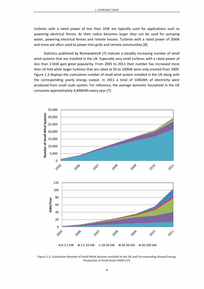
Statistics published by RenewableUK [7] indicate a steadily increasing number of small wind systems that are installed in the UK. Especially very small turbines with a rated power of less than 1.5kW gain great popularity. From 2005 to 2011 their number has increased more than 16 fold while larger turbines that are rated at 50 to 100kW were only erected from 2009. Figure 1.3 displays the cumulative number of small wind system installed in the UK along with the corresponding yearly energy output. In 2011 a total of 104GWh of electricity were produced from small scale system. For reference, the average domestic household in the UK consumes approximately 4,400kWh every year [7].
Figure 1.3, Cumulative Number of Small Wind Systems Installed in the UK and Corresponding Annual Energy Production of Small Scale HAWTs [7]
0
5,000
10,000
15,000
20,000
25,000
30,000
35,000
Num
ber o
f Sm
all W
ind
Syst
ems
0
20
40
60
80
100
120
GW
h/Ye
ar
0-1.5 kW 1.5-10 kW 10-20 kW 20-50 kW 50-100 kW
4

1. INTRODUCTION
When surveying literature it is evident that there is no strict definition for the classification of small scale HAWTs. According to the International Electrotechnical Commission (IEC) [12] turbines with a swept area of less than 200m2 which corresponds to a radius of approximately 8m, are classes as small scale HAWTs. Researchers such as Aner et al. [13] classify turbines with a rated power of less than 50kW as small scale turbines, whereas the RenewableUK allows a significantly higher rated power and sub-divides small scale HAWTs into micro, small and small-medium turbines with a respective maximum rated power of 1.5, 15 and 100kW [7]. Unlike large scale machines, small scale HAWTs are not equipped with control systems to adjust turbine pitch or yaw. Therefore structural features such as the presence of a tail fin to align the rotor with the wind and their ability to self-start have also been used for their classification [14].
1.3 Increasing Underachievement with Decreasing Radius
Although the number of installed small scale turbines, especially those with a rated power of 1.5kW or less, increases rapidly and small scale HAWTs show a lack in performance compared to their large scale counterparts, they have received much less research attention than large scale machines. Companies producing small scale machines are often unable to support R&D on their turbines to the same extent as manufacturers of large machines [8]. This and the cost of production of small scale turbines has led to the cost of electricity generated by small systems being up to 100 times higher than that for large turbines [15]. While the cost of large scale power is approximately 1,300 Euro/kW, the cost for small scale power is in the range of 3,000 to 17,500 Euro/kW. The lack of confidence in the operation of small scale HAWTs has also led to some aid organisations rejecting the use of small scale turbines in village electrification programmes in third world countries [8]. It is therefore the aim of this thesis to address this research gap and contribute to a better understanding and improved performance of small scale HAWTs.
This section reviews the underlying issues that are unique to small scale turbines and act to reduce their performance. The aspects leading to a lower performance have been graphically illustrated in Figure 1.4. Relative to their radius, small scale turbines experience an over proportionally high:
Reduction in Aerodynamic Torque Increase in Resistive Torque
5

1. INTRODUCTION
Figure 1.4, Schematics of Performance Reducing Issues of Small Scale WT’s (Turbine Image from [16])
Reduction in Aerodynamic Torque
Compared to large scale machines, small scale turbines typically experience lower wind velocities and are not able to extract as much power as large turbines from that wind. The unfavourable wind environment small scale turbines are subjected to, is a consequence of their location and much lower altitude. Unlike large scale turbines which operate in relatively steady wind environments, small scale turbines are located where they are required rather than where the wind environment is optimal [17]. According to the RenewableUK [7] the number of small scale turbines has increased 18 fold from 2006 to 2011 in the UK of which 87% were freestanding and 13% were building mounted in 2011, as seen in Figure 1.5. While freestanding turbines only experience velocity variations from the atmospheric Boundary Layer (BL), building mounted rotors are subjected to low wind velocities, high turbulences as well as frequent changes in magnitude and direction of the incoming wind [18]. Uncertainties in the performance predictions are as high as 4-6% for flat terrain and up to 10% for complex terrain [19].
The relatively low energy extraction from small scale blades is a consequence of less optimal blade designs which may result in a comparatively high profile drag but a low lift. The design of small scale turbines is dictated by their consumers who require them to be affordable, reliable and low in maintenance. To meet these criteria the blade’s optimum performance has been sacrificed in favour of its design simplicity and cheap manufacturability.
6

1. INTRODUCTION
Hand carved blades with a high root twist or under-cambered blade profiles for instance become difficult to produce and are subjected to high design uncertainties [20]. The structural integrity of turbine blades further imposes more constraints on the blade design. Blade root sections are required to be thick in order to withstand rotational stresses. Blade profiles with a thickness of 25-30% however have been observed to experience a drastic lift reduction when they operate at low Reynolds numbers (Re) [21]. To avoid the formation of a performance reducing laminar flow separation bubble at low Re, ideally an aerofoil approaching zero thickness is sought [8]. This structural requirement adversely affects the turbine’s performance as it will be seen in later chapters.
Figure 1.5, Trend of WT Siting in the UK [7] and Corresponding Velocity Profiles [7, 22]
The low radius of small scale turbines negatively affects their performance by inducing Reynolds number effects which may be further intensified by low wind speeds. Reynolds numbers below 500,000 are associated with performance reducing flow features [23]. This Re range is typically encountered by turbines with a radius of less than 10m. A detailed discussion of the effect of a reduced radius is presented in section 2.4.2. The reduction of radius is also accompanied by a lower hub height which again is associated with lower wind speeds and higher unsteadiness of the flow. Finally, unlike large scale turbines which are pitch controlled, small scale turbines are stall regulated. This leads to flow separation when they operate at high wind speeds and thereby reduces their power output below the equivalent of a large scale machine [1].
7

1. INTRODUCTION
Increase in Resistive Torque
A wind turbine generator is designed to convert the aerodynamic torque and drive shaft rotation into electricity. However, due to internally generated friction, it generates a resistive torque against the turbine rotation. Micro turbines are typically fitted with a permanent magnet (PM) generator whereas mid-range and mini turbines can also be fitted with an induction generator [8]. Generators impose a resistive or cogging torque on the turbine which decreases at a lower rate than the aerodynamic torque for turbines of decreasing radius [24]. For very low rotational speeds only cogging torques below 1% of the turbine’s rated torque are insignificant [13] but the resistive torque often falls within the range of 1-2% [25]. More details on turbine generators can be found in section 2.3.2.
1.4 Motivation to Investigate Wind Turbine Starting
Similarly to the adverse scaling effects that reduce a small scale HAWT’s performance when it rotates at or near its design operating condition as discussed in section 1.3, there are a number of additional factors that reduce their starting performance and hence further lower their AEY. This section discusses the underlying reasons for the comparatively poor starting performance of small scale HAWTs and hence identifies the niche that this thesis is occupying.
Small scale turbines are often placed in a turbulent environment which leads to more frequent turbine starting than what large scale machines experience. Unlike large scale machines they are often used for short-term power extraction applications such as recharging batteries. This requires them to quickly respond to favourable wind conditions and speed up rapidly to full operational speed to harvest as much energy as possible. Currently, however, small scale turbines are not designed to optimally accelerate from rest [26]. It has consequently been recognised by researchers that small scale WTs have the potential to greatly benefit from an optimisation for a high energy capture at low wind speeds as well as from an optimisation for a quick response to changes in wind direction [18].
Although the demand for a good starting performance of small scale turbines is high, manufacturers impose additional constraints on their design, hindering a quick starting performance, in order to make them more economical. Unlike large scale machines, most small turbines are equipped with generators that are designed to only extract energy, not to accelerate the blades. Small scale turbines therefore solely rely on their aerodynamic torque for starting while experiencing a comparatively high resistive torque from the generator. For turbines with a rated power of less than 50kW it is also not economical to fit them with a pitch control system [13] which could be used to assist turbine acceleration.
8

1. INTRODUCTION
1.4.1 Improving the Understanding of Turbine Starting
Small scale HAWTs undergo a complex start-up sequence when accelerating from rest to full operational speed. The aerodynamics feature low Reynolds numbers in combination with a high angle of attack, α, when the blades start to rotate which leads to a poor performance and is associated with high performance prediction uncertainties. Yet little literature has been published to help the understanding of the complex flow features during the start-up performance of small scale HAWTs. The following research areas have been identified that have not been addressed before:
Analysis of Underlying Flow Features Determining Turbine Starting Performance Systematic Studies on the Effect of Turbine Geometry
Analysis of Underlying Flow Features Determining Turbine Starting Performance
A shortcoming in the current literature is the lack of aerodynamic analysis required to fully understand the starting performance and conclude design recommendations. Turbine starting has initially been investigated through experiments such as the studies conducted by Bechly et al. [27] in 1996. Through these and following experiments validation data was obtained although the experiments were conducted in a field test environment which introduces additional uncertainties, as displayed in Figure 1.6.
Figure 1.6, Uncertainties in the Turbine Wake Structure of the NREL Phase VI Turbine when Comparing Wind Tunnel Experiments with Field Tests [28]
In these experiments, the rotational turbine speed and wind properties were measured which only allows conclusions about the turbine’s tip speed ratio behaviour in time to be
9

1. INTRODUCTION
made. Following, various different versions of the Blade Element Momentum (BEM) theory have been derived to predict turbine starting. The mathematical models often rely on simplifications and empirical formulae as the aerodynamic cL and cD required for BEM models are usually not available for the full range of operating conditions encountered by a starting turbine. Although BEM theory comes with its own limitations and uncertainties, it is a cost effective method of predicting a turbines performance and gives additional information of the torque distribution along the radius. However it does not provide any information on the underlying flow features. This thesis is the first to the author’s knowledge to provide detailed information on the flow as the turbine accelerates using CFD. Through the use of CFD, simplifications, assumptions and uncertainties associated with BEM models are eliminated. The improved understanding of turbine aerodynamics gained by CFD can then be used to improve engineering tools to predict turbine performances such as BEM codes [29], but such studies are outside the scope of this research.
Systematic Studies on the Effect of Turbine Geometry
The limited experimental and computational research done on the starting behaviour of HAWTs has been conducted using different turbines. The turbines investigated varied in their blade profiles, radii and structural properties and have often not been described completely. This makes it difficult to isolate the effect of a single turbine parameter on the starting performance. The present thesis aims to fill this gap by systematically investigating the effect of blade profile, pitch, turbine scale and wind speed by only varying a single parameter at a time and comparing the starting performance to that of a reference turbine. Consequently a design recommendation for turbines of different radii operating at sites with different mean wind speeds and fluctuations can be made.
1.4.2 Potential to Increase Annual Energy Yield
Improving the start-up and low wind speed performance of HAWTs has the potential to significantly increase their AEY. A detailed study conducted by Wright [30] on a rotor with a radius of 0.97m indicated that especially small scale turbines that operate at low wind speeds benefit from an improved starting performance as it can be seen in Figure 1.7. At a wind speed of 4m/s, the AEY can be increased by 8.3% from 290kWh per year to 314kWh per year by optimising turbine starting. At a mean wind speed of 6m/s the improvement drops to 2.5%. Worasinchai [31] argues that the energy yield of a rotor can be increased by as much as 40% when carefully selecting suitable aerodynamic profiles along the blade span to speed up the rotor’s acceleration phase when it accelerates from rest and hence increase the time during which the turbine produces energy.
10

1. INTRODUCTION
Figure 1.7, Estimated Effect of Turbine Starting Performance on Annual Energy Production (Left: Mean vw = 4m/s; Right: Mean vw = 6 m/s) [30]
In section 2.4.5 more details are given on studies that aimed at increasing small scale turbines AEY by improving their starting behaviour. Initial studies that investigated ideal turbine geometries for favourable start sequences, neglected the effect of the modified geometry on the rotors power production when the turbine operates at its design tip speed ratio, λDesign. Only later studies conducted by researchers such as Wood [32] and Clifton-Smith and Wood [33] simultaneously considered the effect of an altered geometry on the turbines starting performance as well as rated power production.
In this thesis the effect of the turbine geometry on its starting performance and power production has been investigated for a range of wind speeds. The aerodynamics of the starting characteristics of small scale HAWTs have been improved by considering the following aspects which increase the chance of a successful turbine start:
• A reduction of the cut-in velocity, vin, of the turbine. This results in a two-fold improvement of the AEY as the turbine starts more frequently and more energy can be extracted from the wind. Particularly turbines which operating in a low wind environment benefit from a low vin as the wind speed at which a turbine ceases to rotate is lower than its cut-in wind speed. This is explained in more detail in section 2.4.1.
• An improved low wind speed and low rotational speed behaviour will lead to a shorter starting time after which the power production commences due to increased rotor acceleration.
In addition to the discussed aims of this thesis the need for more detailed performance specifications for small scale turbines should become clear. Currently the internationally accepted testing standard from the IEC only requires binned wind speed and corresponding power measurements. This crude method of generating the performance curve obstructs the delicate fine details required for the estimation of turbine starting as it does not differentiate
11

1. INTRODUCTION
between rotational speeds when binning the performance data. Alternatively, the commonly quoted λ - Power curve [34] does not contain any information on test wind speeds. As of today there is no standard wind speed at which manufacturers should test their turbines for their power rating [15]. Especially for small scale turbines, this can lead to a misleading performance for both turbine starting and at its design λ performance due to the occurrence of significant Re effects.
1.5 Aims and Objectives
The performance shortcomings of small scale HAWTs compared to their large scale counterparts have been listed in section 1.3 along with the potential benefits of investigating turbine starting in section 1.4. Based on these findings it is the aim of this thesis to quantify the effect of turbine starting of small scale HAWTs on their annual energy yield and consequently recommend favourable blade pitch and thickness designs for maximising the AEY of small scale HAWTs. To the authors knowledge no studies exist in which the effect of turbine starting has been systematically evaluated in a controlled wind environment. This thesis aims to fill this gap by linking the starting performance to underlying aerodynamic flow phenomena dictating the rotors starting behaviour. Furthermore, these systematic studies have been expanded to investigate different diameters of small scale HAWTs which also represent a novel contribution to literature. In order to efficiently tackle these aims, a number of objectives have been defined for this research:
• A literature research on basic wind turbine operation, different computational methods as well as experimental and computational turbine starting investigations has been conducted.
• A fundamental objective of this thesis is the evaluation of computational methods of different complexity along with their strengths and weaknesses. It has been of primary importance that the chosen method complies with the anticipated aerodynamic analysis. The performances of computationally inexpensive blade element momentum models and highly time consuming CFD computations have been evaluated for this purpose. To the author’s knowledge this is the first evaluation of such complexity of different computational methods. It may serve as a useful guideline for researchers investigating the aerodynamic behaviour of turbines with varying rotational speed.
• Aerodynamic comparison methods have been established that allow the flow characteristics to be linked to the turbine’s performance. The aerodynamic performance has been evaluated with respect to the aerodynamic torque and flow features. For a better understanding it was of primary importance to conduct detailed studies of the origin of the total blade torque. Such thorough studies appear to be the first of their kind in published research.
12

1. INTRODUCTION
• Suitable design parameters for the rotor blades that have been analysed have been identified. These parameters either had to significantly affect a small scale HAWT’s starting performance or they had to have received comparatively little research attention. Furthermore different small scale HAWT radii had to be defined. The investigations in this thesis have been conducted at a 0.334m and a 5.029m radius scale with the following blade geometry configurations:
o The NREL Phase VI rotor served as a baseline configuration as outlined by Hand et al. [35]. This turbine also provides an excellent base for the verification of the chosen computational method.
o Increasing the rotor pitch of the reference turbine by 10°. o Reducing the blade thickness of the reference turbine from 0.21c to 0.15c. o Simultaneous rotor pitch increase by 10° and blade thickness reduction from
0.21c to 0.15c. The combination of the two design variation allows an analysis of their interdependence.
• Characteristic starting sequences have been identified for all turbines investigated. • After aerodynamically investigating the different HAWT rotors, a suitable
methodology that relates the turbines start-up performances to their AEY has been established. This methodology was then employed for all wind turbines analysed.
1.6 Thesis Outline
A brief summary of the contents of each chapter in this thesis is given here:
Chapter 1 has introduced small scale HAWTs and clarified the motivation for the research undertaken.
Chapter 2 introduces the necessary background theory on wind turbines that is required for this thesis and assesses the state of the art of literature on turbine starting of small scale turbines, the role relevant geometrical turbine variations and currently employed CFD techniques. The turbine that has been used as a bench mark throughout this work has also been briefly described.
Chapter 3 investigates suitable computational parameters for airfoil and wind turbine simulations. The CFD methods used to simulate turbines operating at a constant rotational speed as well as accelerating from rest are also assessed.
Chapter 4 presents a detailed analysis of the reference blade considering the effect of wind speed and turbine radius as well as their combined effect. The analysis has been conducted with respect to torque, power and flow feature characteristics.
13

1. INTRODUCTION
Chapter 5 shows the results of investigations of the blade geometry at the same wind speeds and turbine radii as in chapter 4. The same analysing techniques as in the previous chapter have been used. Variations in blade pitch, thickness and combined pitch and thickness were considered.
Chapter 6 investigates the effect of the evaluated torque and flow features of all 4 blades from chapter 4 and 5 on their starting performance and consequent annual energy yield in different wind environments. The analysis was conducted for the same turbine radii as in the previous chapters.
Chapter 7 summarises the entire thesis.
14

2. WIND TURBINE THEORY AND LITERATURE
2.1 Introduction
This chapter introduces underlying concepts for the performance of wind turbines which serve as a basis for the remainder of this thesis. It is complimented with a literature review to give the reader an understanding of some historical aspects and introduce the state of the art research on wind turbine performance, starting sequences and relevant computational methods used for their prediction.
At the start of this chapter fundamental wind turbine aerodynamics and relevant structural blade characteristics are presented which are then used to build an understanding of the complex starting behaviour of small scale horizontal axis wind turbines. Literature on the effect of changing the turbine’s geometry has been presented which corresponds to the parameters investigated in chapter 4 and 5, namely turbine scale, pitch and aerodynamic profile. Following is a state of the art literature review of computational fluid dynamics research on airfoil and wind turbine simulations which focuses on the NREL Phase VI rotor. The chapter is finally concluded with a brief description of the NREL Phase VI turbine which served as a reference rotor for the computational methods in chapter 3, the rotor performance analysis in chapter 4, the turbine geometry investigations in chapter 5 and the analysis of the turbine’s self-starting properties in chapter 6.

2. WIND TURBINE THEORY AND LITERATURE
2.2 Fundamental Aerodynamics
In this section, the fundamentals of wind turbine aerodynamics of rotors operating at a constant rotational speed are established. An understating of the complex wind turbine aerodynamics has been built up by first introducing the flow physics around aerofoils and then progressing to wind turbine aerodynamics. This knowledge is essential for the remainder of this chapter as well as for the following chapters.
2.2.1 Aerofoil Flow Physics
As air flows past an aerofoil, it exerts both viscous and pressure forces on the aerofoil. The component of these forces that is aligned with the incoming wind forms the aerodynamic drag and the component perpendicular to the wind forms the aerodynamic lift. The moment of those forces is usually defined around 0.3c of the chord line.
Figure 2.1, Typical Laminar and Turbulent Velocity Profiles Around an Aerofoil [1]
Typical flow structures around an aerofoil are depicted in Figure 2.1. The flow approaching the aerofoil will form a laminar boundary layer at its Leading Edge (LE). Laminar boundary layers are prone to adverse pressure gradients and some aerofoils may form laminar separation bubbles in the Re range of 50,000 to 700,000. The formation of a laminar boundary layer and transition is closely related to hysteresis [36]. Hysteresis is the ability of the flow to remember its history and hence has the potential to produce a different flow field despite the same instantaneous flow conditions. It has been associated with differences in cL and cD of up to 75% and 60% respectively [37]. Aerofoils with a thick camber and round noses typically show hysteresis for Re below 300,000 [38]. Figure 2.2 shows different types of hysteresis of the Lissaman and Miley aerofoils. Detailed flow measurements visualising the hysteresis have been conducted by Yang et al. using Particle Image Velocimetry (PIV) [36]. In the range of 11° < α < 21°, the Lissaman aerofoil experiences a lower cL for decreasing α as the flow attachment occurs at a lower α than the separation when α increases. This trend is reversed
16

2. WIND TURBINE THEORY AND LITERATURE
for the Miley aerofoil which makes it more suitable for turbine starting where α decreases in time, as indicated by the red arrow.
Figure 2.2, Different Types of Hysteresis for the Lissaman 7769 and the Miley M06-13-128 Aerofoils at Re = 150,000 [36, 38]
A laminar boundary layer breaks down into a turbulent one when small harmonic waves in the flow become unstable due free stream turbulences, acoustic waves or surface roughness. The newly formed turbulent boundary layer exerts a higher shear stress on the wall and therefore increases cD for a fully attached boundary layer. Mueller et al. [23] experimentally observed that moving the transition point 10% closer to their aerofoil’s Trailing Edge (TE) caused a 10% decrease in the drag. However, due to the higher momentum of a turbulent boundary layer it is more resistant to adverse pressure gradients and therefore less likely to cause flow separation than a laminar boundary layer. This can result in less form drag.
17

2. WIND TURBINE THEORY AND LITERATURE
2.2.2 Wind Turbine Flow Physics
The understanding of the flow physics of a wind turbine which dictates its performance has been built up progressively in this section. Initially basic relations between the turbine’s geometry and performance are introduced which are then extended to cover rotational effects and unsteady flow features. Finally an overview of different torque classifications which have been used extensively in the following chapters is given. This section is structured as follows:
Turbine Geometry on Performance Rotational Effects Hysteresis Turbine Torque Classifications
Turbine Geometry on Performance
A HAWT’s performance is linked to the tip speed ratio λ at which it operates in a similar manner in which an aerofoils performance depends on α. The definition of λ is given in Equation 2.1.
The local aerodynamic performance of a wind turbine is dictated by the particular Re and α distribution along the wind turbine’s blade in combination with its geometry. However the flow around a wind turbine is more complex than that around an aerofoil, as each aerofoil section along the blade span experiences a different α and Re for a turbine that experiences a uniform wind and rotates at a constant rotational speed. Additionally, 3D flow effects are introduced by the radial Re and α gradients, the air displacement of the turbine hub, the blade rotation itself and the tip vortices. The complex radial Re and α distributions are a result of the blade geometry and the magnitude and direction of the relative velocity vrel. Vrel in turn depends on the uniformly distributed wind speed, vw and the linearly distributed rotational velocity, vrot. This is illustrated in Figure 2.3 for the NREL Phase VI turbine operating at λ = 5. The blade tip experiences a high vrel at a relatively small angle to the rotational plane which encourages favourable aerodynamic coefficients. The component of cL and cD of each aerofoil section in the rotational plane along with the aerofoil’s offset from the centre of rotation generate the aerodynamic turbine torque which can either be used to produce power or accelerate the turbine. In contrast to the blade tip, the blade root experiences a low vrel at a relatively large angle.
𝜆𝜆 =𝑅𝑅𝑅𝑅𝑣𝑣𝑤𝑤
Equation 2.1
18

2. WIND TURBINE THEORY AND LITERATURE
Figure 2.3, Geometrical Velocity Component along the Blade Span of the NREL Phase VI Turbine Determining the Local Re and α at λ = 5
Although the NREL Phase VI turbine has a linear radial chord distribution, see Figure 2.32, the radial Re distribution is non-linear due to the span-wise non-linearity of the magnitude of vrel. For most tip speed ratios however α shows a stronger span-wise non-linearity than Re. This is because of the non-linear twist distribution of the NREL Phase VI blade and the non-linearly changing span-wise angle between vrel and the rotational plane despite the linear vw and vrot distributions. This radial non-linearity of the geometric α and Re pattern is depicted in Figure 2.4 for a λ of 0 to 6 as the rotor operates at a wind speed of 6m/s. The geometric Re and α patterns presented do not account for induced velocities and can therefore only be used as a guideline. Especially at high λ, the geometric Re is an overestimation of the actual Re but for the sake of demonstration it is sufficient for this thesis. Figure 2.4 also schematically shows the geometric Re and α drawn to scale at r/R = 0.3 and 0.9 when λ = 0, 3 and 6. It is important to note that when maintaining λ, a change in vw only affects Re, not α.
19

2. WIND TURBINE THEORY AND LITERATURE
Figure 2.4, Contours Showing Geometrical Re and α for the Full Scale NREL Phase VI Blade operating at vw = 8m/s from λ 0 to 6 and Geometric Re and α Drawn to Scale for r/R = 0.3 and 0.9 when λ = 0, 3 and 6
For a given radial section, an increase of λ is associated with an increase of Re while α decreases. This however occurs at different rates for different r/R, making the Re and α patterns complex. When the blade is stationary, the Re at the blade root exceeds that of the blade tip while the root also experiences a more favourable α. As λ increases the Re at the blade tip becomes larger than that of the blade root and the flow incidence angle at the blade tip becomes smaller than that of the blade root. The effect this has on the power producing sections of the blade is shown in Figure 2.5. Rohrbach et al. [39] experimentally investigated the power generation of their turbine when incrementally removing blade sections from the root. The resulting drop in the monitored power is due to the reduced blade area. Although their power measurement of the mounted blade sections is slightly underestimated due to the formation of an additional tip vortex at the inner edge of the cut out section and due to the additional drag of the exposed shaft. At a λ = 10 the majority of the power was generated by the upper half of the blade. From root to tip, the blade sections between r/R = 0.1, 0.25, 0.35, 0.5 and 1 generated 8, 11, 21 and 60% of the power respectively.
20

2. WIND TURBINE THEORY AND LITERATURE
Figure 2.5, Power Generation When Omitting Different Blade Sections from the Root of a Turbine with R = 29m [39]
Rotational Effects
For an intuitive representation of the flow features, the flow features have been analysed in a rotating reference frame in this thesis. In order to convert from a stationary, inertial reference frame to a rotating, non-inertial reference frame the following forces are required:
• Coriolis force: acts perpendicular to the streamline direction in the plane of rotation • Centrifugal force: acts radially outwards • Euler force: only present when turbine accelerates
Figure 2.6, Rotational Effects on Streamlines of Flow around the NACA 0018 (Left: Blade Cross-Section at r/R = 0.16; Right: Stationary Aerofoil at Equivalent Re and α) [40]
21

2. WIND TURBINE THEORY AND LITERATURE
Both, the Coriolis and centrifugal force have been shown to play an important role in 3D stall delay [40, 41]. Figure 2.6 shows their effect on a section of rotating blade and a stationary aerofoil operating at equivalent Re and α. The streamline pattern of the wind turbine cross-section shows a separation bubble of a much lower thickness than that of the equivalent 2D aerofoil as the air is redistributed radially outwards. The reduction of the size of the separation bubble increases the blade loading by creating a larger pressure drop on the Suction Surface (SS) [42]. This results in a high increase of cL and thereby improves the turbines performance [40]. The Coriolis force plays an especially important role at the blade root, due to the massive flow separation caused by the large α at low rotational speeds or low λ.
Hysteresis
In section 2.2.1 the source of flow transition and hysteresis on aerofoils as well as their effect on cL and cD has been discussed. The Re and α at which these flow phenomena occur for a selection of aerofoils have been summarised in Table 2.1. The data was used to indicate which radial sections of wind turbines may be subjected to flow transition or hysteresis effects as the turbine operates at different λ. Figure 2.7 shows the results for a turbine with the chord and twist distribution of the full scale NREL Phase VI turbine operating at a wind speed of 6m/s. From λ ≈ 1 to λ ≈ 8 the turbine may experience flow transition or hysteresis effects although hysteresis effects appear to occur over a narrower λ range.
Figure 2.7, Radial Locations where Flow Transition or Hysteresis Effects are Likely to Occur at Different λ using Data from Table 2.1 and Radial Chord and Twist Distribution from the NREL Phase VI Blades, R = 5.029m,
vw = 6m/s
22

2. WIND TURBINE THEORY AND LITERATURE
Phenomena Aerofoil Re x 103 α [°] Reference(s)
Flow Transition
NACA 0012 5.3-51 0-90 Alam et al. [43] NACA 0018 150-1,000 10-27 Timmer [44] NACA 654-421 200-600 10-40 Devinant et al. [45] NACA 0012 360-760 10-30 Alam et al. and References [43]
Hysteresis
Miley 70-150 10-18 Pohlen and Mueller [37] Miley M06-13-128 Lissaman 7769
100-150 150-290
8-18 8-18
Mueller [38]
GA(W)-1 160 13-16 Yang et al. [36] S6074 200 11-19 Selig [46] NACA 0018 300-700 12-24 Timmer [44]
Table 2.1, Experimentally Observed Flow Conditions Associated with Flow Transition and Hysteresis
Turbine Torque Classifications
This section is concluded with the definitions of the commonly used non-dimensional torque and power coefficients in Equation 2.2 and Equation 2.3 and an overview of different classifications of the turbine torque in Table 2.2 along with a brief description. The table is designed to serve as a reference for the following chapters.
𝑐𝑐𝑃𝑃 =𝑃𝑃𝑜𝑜𝑜𝑜𝑜𝑜
12𝜌𝜌𝜌𝜌𝑅𝑅
2𝑣𝑣𝑤𝑤3 Equation 2.2
𝑐𝑐𝑇𝑇 =
𝑇𝑇𝑛𝑛𝑛𝑛𝑜𝑜12𝜌𝜌𝜌𝜌𝑅𝑅
3𝑣𝑣𝑤𝑤2 Equation 2.3
Symbol/Equation Description 𝑇𝑇𝑛𝑛𝑛𝑛𝑜𝑜 = 𝑇𝑇𝑎𝑎𝑛𝑛𝑟𝑟𝑜𝑜 − 𝑇𝑇𝑟𝑟𝑛𝑛𝑟𝑟 Net Torque produced by WT at specific λ
𝑇𝑇𝑟𝑟𝑛𝑛𝑟𝑟 Total resistive torque of generator, explained in more detail in section 2.3.2
𝑇𝑇𝑎𝑎𝑛𝑛𝑟𝑟𝑜𝑜 Total aerodynamic blade torque at specific λ
𝑇𝑇𝑎𝑎𝑛𝑛𝑟𝑟𝑜𝑜 = 𝑇𝑇𝑃𝑃𝑃𝑃 + 𝑇𝑇𝑃𝑃𝑃𝑃 Aerodynamic Torque produced by pressure and suction surface
𝑇𝑇𝑎𝑎𝑛𝑛𝑟𝑟𝑜𝑜 = 𝑇𝑇𝑃𝑃 + 𝑇𝑇𝑣𝑣𝑣𝑣𝑟𝑟 Pressure and Viscous Torque
𝑇𝑇𝑎𝑎𝑛𝑛𝑟𝑟𝑜𝑜 = �𝑇𝑇𝑣𝑣 Aerodynamic torque over cell i, only used for CFD
𝑇𝑇𝐴𝐴(𝑣𝑣) =𝑇𝑇𝑣𝑣
𝑇𝑇𝑎𝑎𝑛𝑛𝑟𝑟𝑜𝑜 𝐴𝐴𝑣𝑣� Torque per unit area, explained in detail in section 4.2.1
Table 2.2, Overview of Different Torque Classifications
23

2. WIND TURBINE THEORY AND LITERATURE
2.3 Relevant Structural Properties of Wind Turbines
The structural properties of the turbine blades and the generator play a comparatively insignificant role when the turbine rotates at constant rotational speed at or near its design λ. But they have a significant effect on the starting performance of a rotor. Turbine inertia and generator characteristics have therefore been discussed in detail in this section.
2.3.1 Turbine Inertia
The inertia, I, of the turbine blade and generator act to inhibit the acceleration of the blade. Its definition is given in Equation 2.4.
𝐼𝐼 = � 𝑟𝑟𝑣𝑣2𝑚𝑚𝑣𝑣 𝑑𝑑𝑟𝑟
𝑅𝑅
0 Equation 2.4
To derive the inertia of turbine blades it is essential to know the material(s) the blade is made off and their detailed distributions inside the blade. Wind turbine blades of a radius of up to 2.5m are often made of solid homogenous materials, such as timber. Blades with a larger radius however are frequently made of shell structures with laminated composites to create sufficiently strong but lightweight blades [8]. This is illustrated in Figure 2.8 for the NREL Phase VI turbine which has a radius of 5.029m.
Figure 2.8, Cross-Section of the NREL Phase VI Turbine Blade [35]
Although the turbines considered in this thesis have a radius of up to 5.029m, for inertia calculations all blades investigated have been assumed to be composed of the same, homogenous material. The following relations between the turbine geometry and inertia can therefore be made:
• Dependence on radius: 𝐼𝐼 ∝ 𝑅𝑅5 Equation 2.5
• Dependence on blade thickness, tb: 𝐼𝐼 ∝ 𝑡𝑡𝑏𝑏 Equation 2.6
24

2. WIND TURBINE THEORY AND LITERATURE
2.3.2 Generator
Large scale turbines are commonly equipped with a wind speed sensor that activates the generator to accelerate the rotor when the turbine is stationary and the wind speed is sufficiently high. Most small scale machines however are equipped with a generator that can only extract energy from the wind for constructional simplicity. They therefore solely rely on their aerodynamic torque for starting [8].
The effect of the generator on a wind turbine’s performance depends on both, the generator’s efficiency and its resistive torque. The amount of resistive torque exerted by the generator depends on the type of generator used, its rated size and configuration. The net torque available for power production or turbine acceleration is the difference between the aerodynamic torque and the resistive generator torque, Tres.
𝑇𝑇𝑛𝑛𝑛𝑛𝑜𝑜 = 𝑇𝑇𝑎𝑎𝑛𝑛𝑟𝑟𝑜𝑜 − 𝑇𝑇𝑟𝑟𝑛𝑛𝑟𝑟 Equation 2.7
Turbines with a radius of less than 1.5m are commonly fitted with a PM generator, above that radius PM or induction generators are often used [8]. PM generators rated at 500W and 1.5kW typically impose a cogging torque of 0.3 and 0.6Nm respectively on the stationary blades [47]. When the blade is stationary the generator torque exerts a comparatively high static resistive torque which drops to a lower dynamic value once the turbine starts to rotate. Wright and Wood [48] observed a drop from 0.36 to 0.24Nm for their 600W machine. For more characteristic torques refer to Table 2.3.
Generators of small scale HAWTs typically begin with their power extraction when the turbine shaft reaches a fixed fraction of the maximum rotor speed which is determined by the control system [13, 30]. Power extraction is therefore independent of wind speed. Generator efficiency improves for high wind speeds [17] and commonly reaches values of 93 to 94% [49]. Due to the lack of detailed generator information, the generator was assumed to only extract power when the turbine operates at its design λ in this thesis.
2.4 Starting of Small Scale HAWTs
Small scale HAWTs undergo a complex starting sequence that has not been addressed adequately in literature. This section introduces the basic concepts of turbine starting by considering fundamental wind turbine aerodynamics as introduced in section 2.2.2 and relevant structural characteristics which have been evaluated in section 2.3. After introducing typical starting sequences at low and high wind speeds, the effect of scaling a turbine, altering the blade’s pitch and aerodynamic profile has been evaluated. To allow for a meaningful comparison between turbines of different radii operating at different wind speeds, the turbine performance has often been presented in non-dimensional form.
25

2. WIND TURBINE THEORY AND LITERATURE
The starting sequences and characteristics from a total of 15 publications have been reviewed. Table 2.3 summarises the available data for turbines analysed in this chapter, already indicating the incomplete nature of the available data.
Rese
arch
er(s
)
Radi
us [m
]
Num
ber o
f Bl
ades
Roto
r Ine
rtia
[k
gm2 ]
Resis
tive
Torq
ue [N
m]
Rate
d Po
wer
[k
W]
Cut i
n ve
loci
ty
v in [m
/s]
Data
Sou
rce
Bechly et al [27] Ebert and Wood [17] Clausen and Wood [14] Hampsey and Wood [26] Mayer et al [50]
2.5 2 ≈12.06 5 Field tests
Clausen and Wood [8] 2 20 3.5 Field tests Clausen and Wood [8] 3 0.4 0.6 2.75 Field tests Wright and Wood [48] Wright [30]
0.97 3 0.43 Static 0.36
Dynamic 0.24 0.6 4.8 Field tests
Ozgener and Ozgener [51]
1.5 3 1.5 2.4 Field tests
Worasinchai [31] 1.2 2.6 (SG) 2.0 (MX,
MP)
Static 0.45 Dynamic 0.3
1 Simulations
Clausen et al. [20] 0.9 3 0.5 3.5 Field tests Aner et al. [13] 2.5 2 18 5.6 2.5 Simulations Kishore [52] 0.20 3 Experiment Hand et al. [35] 5.029 2 949 19.8 6 Experiment
Table 2.3, Structural and Aerodynamic Properties of Turbines used for Start-Up Investigations by Other Researchers
Bechly et al. [27] can be considered as the pioneers in wind turbine starting research. In 1996 they designed and tested small scale HAWT blades that had been used by several fellow researchers to investigate turbine start-up behaviour. Their blade also served as design basis for other turbine blades. Clausen and Wood [8], Wright and Wood [48] and Wright [30] scaled Bechly’s blades down to a 600W scale, increased the relative chord by 40% and pitched the blade by 5°. Clausen et al. [20] later analysed an identical turbine to the one from Wright and Wood [48] but with turbine blades that were hand carved. Clausen and Wood [8] also worked on a 20kW scaled up version of Bechly’s blades. Other researchers designed their blades independently. The findings of each of the researchers work has been presented in the following sub-sections where adequate to allow for a subject-orientated structure of this section.
26

2. WIND TURBINE THEORY AND LITERATURE
2.4.1 Analysing Typical Starting Sequences
The starting sequence of free standing wind turbines is highly complex due to their encounter with low Re combined with high α, a high turbulence level and an unsteady flow environment. In order to gain an overview of this process, relevant literature investigating aspects of turbine starting is presented along with the fundamental wind turbine aerodynamics that have been established in section 2.3. For an easier understanding, the current section first gives an overview of turbine starting, then divides starting sequences into distinct, characteristic stages and finally gives an example of a turbine start at a high and a low wind speed during field tests. The mean wind speeds of the starting sequences were approximately 9 and 4.5m/s. This section is divided into the following sub-sections:
Overview Distinct Starting Stages Example: High Wind Speed Start Example: Low Wind Speed Start
Overview
The schematics of a rotors response to the incoming wind speed are shown in Figure 2.9. More details on each section of the graph are provided in the remainder of this section. The following parameters are important for a small scale HAWT that is subjected to a fluctuation wind:
• The cut in velocity, vin, is the wind speed at which rotation is initiated. The turbine begins to accelerate thereafter until it reaches its design λ provided that the wind speed does not drop to a too low value below which no positive torque can be generated. As it will be shown later turbine starting may be completed even when the wind speed moderately decreases.
• When the rotor operates at a sufficiently high ω the generator is engaged and the turbine produces power. In this thesis the generator has been assumed to engage only when the turbine operates at its design λ.
• The cut out velocity, vout, has been defined as wind speed at which the turbine cannot generate a positive net torque anymore. This is in contrast to the more commonly used definition of the wind speed at large scale turbines have to be shut down in order to prevent damage. The present definition is more suitable for small scale HAWTs as they are stall regulated to prevent generator overloading and do not possess over active blade pitch control mechanisms to shut the rotor down. When a small scale HAWT is subjected to vout, the rotor will slow down until the blade rotation ceases.
27

2. WIND TURBINE THEORY AND LITERATURE
Figure 2.9, Schematics of Turbine Response to Wind Speed
The fundamentals of turbine starting are introduced focusing on the turbine starting analysis of Wright and Wood [48] and Wright [30]. In both publications the same 3 bladed turbine with a radius of 0.97m has been investigated, see Table 2.3 for more details. This particular turbine was chosen as a reference as Wright and Wood [48] performed by far the most detailed turbine starting investigations and presented the completest turbine description. For their computational analysis they used a modified BEM theory which has been explained in section 2.5. Figure 2.10 shows the result of Wright and Wood’s [48] BEM predictions indicating at which rotational speed and wind speed combination the turbine accelerates or decelerates. The figure will be interpreted in more detail when discussing the distinct starting stages.
Figure 2.10, Estimated Steady Rotor Performance Curve for Different vw and ω [48]
28

2. WIND TURBINE THEORY AND LITERATURE
Wright [30] also compared his measured starting time of 665 starting sequences with different computational models as shown in Figure 2.11. A complete turbine start was defined as the time taken from rotation initiation until the generator begins with the power extraction at a rotational speed of at least 268rpm. The duration of the starting sequences ranges from 6.9s at high wind speeds to 169s at low wind speeds with an average of 35.3s. The starting time TS shows an inverse relationship to the wind speed, see Equation 2.8. This is in agreement with torque dependence on the wind speed in Equation 2.3. The wider spread of starting times at low wind speeds is a likely consequence of low Re effects. The increasing deviation between the starting time predictions of the computational models and experimental measurements at low wind speeds could be caused by high uncertainties in the performance predictions of aerofoils operating at low Re. This has been observed even under steady conditions [17].
𝑇𝑇𝑟𝑟 ∝ 𝑣𝑣𝑤𝑤−2 Equation 2.8
Figure 2.11, Length of Starting Sequence as Function of Mean Wind Speed [48]
Distinct Starting Stages
Although the starting performance of a turbine varies largely depending on its aerodynamic and structural properties and its wind environment, starting sequences can be divided into the following distinct stages:
• Rotation initiation • Idling period • Final acceleration
A stationary turbine experiences high α along its span of up to 90°. The unfavourable flow conditions, characterised by low Re and high α, are schematically illustrated in Figure 2.4
29

2. WIND TURBINE THEORY AND LITERATURE
for a stationary turbine at r/R = 0.3 and 0.9. When the turbine faces the incoming wind perpendicular to its rotational plane, its starting torque will only depend on cL and is independent of cD. Due to the blade twist, the blade root experiences the lowest α but even there the blade will experience stalled flow which considerably reduces cL. This leads to a low turbine torque which is typically several orders of magnitude lower than that of a turbine operating at its design λ. Nonetheless, the turbine has to generate enough aerodynamic torque to overcome the static resistive torque of the generator and drive train in order to start rotating. The generator has been described in more detail in section 2.3.2 and characteristic resistive torque values are given in Table 2.3.
Wright [30] experimentally observed his turbine to start rotating at an average wind speed of 4.8m/s, although rotation initiation was also observed for wind speeds from 1.9 to 7.9m/s as shown in Figure 2.12. Most turbine starts occurred when the wind accelerated, a few however were observed for a decelerating wind. No explicit reasoning has been given for this behaviour but the limited response of his experimental apparatuses may have obscured some trends. Ebert and Wood [17] also argue that the use of a single cut in wind speed is too simplistic. A summary of averaged cut in wind speeds which range from 2.8 to 6m/s for different turbines is listed in Table 2.3.
Figure 2.12, Measured Starting Wind Speed and Wind Acceleration When Turbine Rotation is Initiated [30]
Once the turbine rotates, the rotor is subjected to a lower dynamic resistive torque. According to Wright and Wood’s [48] mathematical model which is illustrated graphically in Figure 2.10, the difference of 0.12Nm between their static and dynamic resistive generator toque, is responsible for the shift of the cut in wind speed from 4.2 to 5.1 m/s. When the blade starts to rotate it experiences an additional velocity component vrot which increases from the root to the tip as depicted in Figure 2.3. This increases the relative velocity vrel experienced by the blade while decreasing the local α, which in turn acts to accelerate the blade due to the
30

2. WIND TURBINE THEORY AND LITERATURE
favoured flow environment. The turbine acceleration is linked to its net torque and inertia as stated in Equation 2.9.
𝑇𝑇𝑎𝑎𝑛𝑛𝑟𝑟𝑜𝑜 − 𝑇𝑇𝑟𝑟𝑛𝑛𝑟𝑟 = 𝐼𝐼𝑑𝑑𝑅𝑅𝑑𝑑𝑡𝑡
Equation 2.9
Due to the complex aerodynamics, successful turbine starting sequences have been observed for decreasing wind speeds. According to Figure 2.10 Wright and Wood’s [48] turbine can sustain an increase of its rotational speed for a relatively rapidly dropping wind speed, provided the turbine rotates at more than approximately 50rpm. Below that rotational speed the turbine will cease to rotate. The graph also indicates that the cut out wind speed at which the rotor cannot sustain its rotational speed of 2.5m/s is significantly lower than its cut in wind speed of 5.1m/s. This phenomenon has been reported multiple times in literature [17, 24]. As a consequence using the IEC standards for determining the cut in velocity of a small scale HAWT by binning 1min performance averages will underestimate the cut in velocity [24, 53] and therefore overestimate the turbines annual energy yield.
Depending on the wind speed and the turbine’s rotational speed, the turbine can enter a long idling period. During that period the Re and α at which the turbine operate only change at a low rate. This phase usually lasts quite long for turbines that are designed for an optimal power output at full operational speed as the blade’s α decreases at a low rate due to the low torque generation at low λ [8]. Mayer [50] and Ebert and Wood [17] report idling times of 30 to 50s. Once α drops to a value approaching the aerodynamic profile’s maximum cL/cD, the turbine begins to accelerate rapidly and subsequently ends the starting phase [8].
Example: High Wind Speed Start
A typical starting sequence of Wright’s [30] turbine as it is subjected to an average wind speed of approximately 9m/s is illustrated in Figure 2.13 along with α, Re and local blade torque at the blade root and tip. The author acknowledges that the prediction of α may not be highly accurate due to complex 3D stall phenomena.
The turbine rotation is initiated at a wind speed of approximately 5.5m/s. The following increase in the wind speed ensures that the turbine stays within the envelope of the ‘area of rotor acceleration’ in Figure 2.10 throughout its entire starting sequence. This promotes rapid turbine acceleration, eliminates the idling phase and results in nearly linear turbine acceleration until the start-up phase is completed.
The wind velocity pattern is clearly reflected in the Re trend at the blade root but only mildly shows in the blade tip Re distribution. α along the blade appears relatively unaffected. Consequently the blade root produces most of the torque as the wind speed is very high when the turbine starts to rotate but is overtaken by the torque production at the tip when the wind velocity decreases approximately 6s after rotation is initiated. At this time α at the blade tip reduced to about 30° which is far better for a high torque production than the α of 55° at the blade root.
31

2. WIND TURBINE THEORY AND LITERATURE
Figure 2.13, Measured and Predicted Turbine Rotational Speed, Predicted Reynolds Number, Angle of Attack and Torque for a High Wind Speed Start [30]
Example: Low Wind Speed Start
During the low wind speed starting sequence in Figure 2.14, the turbine experienced an average wind speed of approximately 4.5m/s with a minimum wind speed of 2.4m/s after rotation initiation. These low wind velocities cause the turbine to mildly accelerate and decelerate as it frequently leaves the ‘area of rotor acceleration’ envelope of Figure 2.10 and thereby induces a long idling time of approximately 80s. A low cL to cD ratio at low Re is largely responsible for the poor starting performance [8].
Similarly to the high wind speed start, the wind speed pattern is reflected in the Re number at the blade root but not at the tip. The reduction in wind speed however cause the wind speed pattern to also show up in the α trend, especially at the blade tip. This makes the turbine’s torque response along its entire radius highly unsteady. The blade tip begins to generate a higher torque than the blade root only at approximately 79s after rotation
32

2. WIND TURBINE THEORY AND LITERATURE
initiation. The sharp increase of the torque at the tip thereafter causes the turbine to rapidly accelerate and complete its starting phase.
Figure 2.14, Measured and Predicted Turbine Rotational Speed, Predicted Reynolds Number, Angle of Attack and Torque for a Low Wind Speed Start [30]
2.4.2 Effect of Turbine Scale
The diameter of the turbine affects its performance in several ways. Figure 2.15 shows a comparison between the starting performance of a 600W machine investigated by Hampsey and Wood [26] and Clausen and Wood [14] and a 5kW turbine analysed by Wright [30]. Details on each turbine are presented in Table 2.3. Although the starting behaviour of the turbines in Figure 2.15 is dominated by the effect of the turbine radius, other parameters such as a different blade geometry and wind environment will also affect their starting behaviour.
33

2. WIND TURBINE THEORY AND LITERATURE
Figure 2.15, Effect of Turbine Scale on Rotor Starting Performance
The starting performance of the smaller machine is clearly seen to outperform that of the larger turbine. The idling period for the larger 5kW rotor lasts until the rotor reaches λ ≈ 4 and is characterised by a low increase of the rotational speed. The 600W machine shows a much higher initial acceleration and progresses to its final acceleration phase when λ ≈ 1.6. The final dλ/dt acceleration gradient for both turbines is relatively similar. This is in agreement with findings from Maeda et al. [54] who conducted field tests on a 10m diameter HAWT and wind tunnel test on smaller turbine. From their experiments they concluded that when the local α is below that corresponding to static aerofoil stall, both wind turbines deliver a similar performance. Following is an overview of the radial dependence of parameters relevant to turbine starting and an analysis of their significance:
• Reynolds Number 𝑅𝑅 • Power Output 𝑅𝑅2 see Equation 2.2 • Starting Torque 𝑅𝑅3 see Equation 2.3 • Inertia of Blades 𝑅𝑅5 see section 2.3.1
The theoretical scaling effect of a turbine on its dλ/dt acceleration can be evaluated from Equation 2.9 and Equation 2.1 as illustrated in Equation 2.10. From theoretical considerations the dλ/dt acceleration of the 600W machine should be approximately 2.5 times higher than that of the 5kW machine which can be approximately observed for the initial acceleration phase of the turbines in Figure 2.15.
34

2. WIND TURBINE THEORY AND LITERATURE
𝑑𝑑𝜆𝜆𝑑𝑑𝑡𝑡
∝𝑅𝑅𝑇𝑇𝐼𝐼∝𝑅𝑅𝑅𝑅3
𝑅𝑅5= 𝑅𝑅−1 Equation 2.10
Reynolds Number
For identically shaped blades, the Reynolds number scales linearly with radius. A decreasing Re is associated with a reduction of the aerodynamic force, a decrease of the maximum obtainable cL/cD ratio [55] and hysteresis effects. As described in section 2.2.1, hysteresis related Re effects typically occur below a chord Reynolds numbers of 300,000. Figure 2.16 shows the radial sections at which turbines with a radius of 0.34, 5 and 10m with a chord and twist distribution of the NREL Phase VI turbine as shown in Figure 2.32, would be likely to encounter hysteresis or transition effects as they operate at different wind speeds using the aerofoil data from Table 2.1. The 0.34 and 5m radius turbines may experience flow transition and separation effects over a wide range of λ, including at their design λ at low and high wind speeds. Only the 10m radius machine experiences insignificant Re effects when it operates at wind speeds above 10m/s. A turbine that experiences dynamic stall effects requires a longer starting time as its rotor acceleration is reduced [48].
Figure 2.16, Operating λ and r/R at which a Turbine with Chord and Twist Distribution of the NREL Phase VI Turbine at Scale R = 0.34, 5 and 10m Operating at vw = 3 and 10m/s May Encounter Hysteresis and Flow
Transition Effects
35

2. WIND TURBINE THEORY AND LITERATURE
Re effects have the potential to significantly reduce a turbine’s power output. Experimental investigations of 3 different turbines, namely ‘AF15’, ‘AF30’ and ‘AF60’, each at a 2.4, 30 and 60m radius by Rohrbach et al. [39], indicated that the smallest sized turbines suffered from a significant power output reduction due to Reynolds number effects as seen in Figure 2.17. The reduction in efficiency implies that small turbines will have a lower acceleration rate from a purely aerodynamic point of view.
Figure 2.17, Effect of Reynolds Number on Power Output for 3 Turbines at 2.4m, 30m and 60m Radius Scale [39]
Starting Torque
The starting torque theoretically scales with 𝑅𝑅3. The actual net torque generated by a small scale turbine however will scale at a different rate because:
• The generated aerodynamic torque will be below its expected value due to Re effects as outlined in the previous section.
• The resistive torque imposed by the generator and drive train decreases at a lower rate than 𝑅𝑅3 [24].
These factors make it more difficult for a turbine to generate a positive net torque as the turbine radius decreases. Micro turbines face the biggest challenge in generating enough torque to start rotating. Resistive torques as low as 0.2Nm were found to have a significant effect on the starting performance of micro turbines [32]. To counteract this torque deficit, micro turbines commonly have many blades. Their cut in wind speed however can still be above 5m/s [8]. Increasing the number of blades will narrow the λ range over which the blade produces power and shift the optimum performance to a lower λ [1]. Wood [24] illustrated
36

2. WIND TURBINE THEORY AND LITERATURE
the effect of the resistive torque on the start-up of his 5kW machine. He observed that an increase in the resistive torque from 1Nm to 2.5Nm was accompanied by an increase of the cut in wind speed from less than 3m/s to well over 4m/s. Similarly, Wright [30] estimated that the 0.12Nm difference in static and dynamic torque requires a minimum wind speed of 5.2m/s instead of 4.2m/s as it can be seen in Figure 2.10.
It can be concluded that the rotation initiation is most difficult for micro turbines, once a turbine is rotating however larger turbines tend to idle longer due to a lower rotor acceleration.
2.4.3 Effect of Blade Pitching
It has been observed experimentally, that the blade pitch angle significantly affects a turbine’s starting performance as well as its design λ performance. A stationary un-pitched blade will experience the incoming wind at α equivalent to 90° − 𝛽𝛽𝑜𝑜𝑤𝑤𝑣𝑣𝑟𝑟𝑜𝑜. This results in a combination of high α and low Re which causes large parts of the blade to be covered by stalled flow. This stall reduces the blade’s performance and creates an unsteady flow field that is highly sensitive to the flow environment [48]. Twisting or pitching the blade reduces the local α and thereby increases the generated torque.
Figure 2.18, Effect of Blade Pitch on Rotor Starting Performance
37

2. WIND TURBINE THEORY AND LITERATURE
Figure 2.18 shows the comparison of the experimentally derived starting sequences of a 5kW turbine operating in 3 different pitch configurations. Ebert and Wood [17] fitted a pitch adjustment mechanism to their turbine so that the blades were highly pitched when the turbine just started to rotate. The wind and blade rotation forces then acted to reduce the pitch angle as the blade gains rotational speed. This reduces the local α to a lower value than those encountered during a fixed pitch angle start and hence results in the best starting performance. The turbine shows a similarly good performance for the experiments conducted at a fixed pitch angle of 35° for the first few seconds before it stops accelerating and idles at λ ≈ 2. The un-pitched blade in contrast shows a much lower acceleration during the first few seconds but steadily continues to accelerate until the blade reaches a λ of 4 before it rapidly accelerates. In contrast to this, Wright [30] observed that pitching his 600W blade by only 5° did not have any significant effect on its resulting performance. Mayer et al. [50] who tested their turbine for a fixed blade pitch between 0 and 35°, observed that a pitching angle of 20° resulted in the shortest starting sequence.
Figure 2.19, Effect of Blade Pitch on Torque and Power of the WKA-60 Turbine [1]
38

2. WIND TURBINE THEORY AND LITERATURE
More systematic pitching angle performance studies are shown in Figure 2.19 although they do not examine turbine starting behaviour. Hau [1] presented power and torque coefficients for different λ of the WKA-60 turbine when it was set to operate at fixed blade pitch angles ranging from 2 to 40°. The torque coefficient indicates that the torque at low λ is significantly improved the more the blade is pitched which is in agreement with the trend of the observed starting sequences in Figure 2.18. An increased blade pitch however is accompanied by a reduction of the torque peak which is also shifted towards lower λ. This implies that the blade would greatly benefit from high pitch angles at low λ when accelerating from rest. However after it has reached its maximum torque producing λ, a high pitch angel works to the blade’s disadvantage as the torque not only reaches a lower torque peak but also begins to drop more rapidly for high pitching angles. A high pitch angle also causes a reduction in the blades maximum power coefficient. More pitching angle investigations are provided by Rohrbach et al. [39]. A comparison of the literature shows that the dependence of cT and cP on λ and turbine pitch is highly affected by the turbine’s geometry.
2.4.4 Effect of Blade Profile
Modifying a turbine’s aerodynamic profile will both alter the torque generated by the turbine as well as its inertia. While thin aerofoils are generally desirable due to their high cL/cD ratio they cannot be used in the blade root section due to structural constraints. More details on structural constraints are provided in section 1.3.
Worasinchai [31] performed a detailed study on the effect of the use of different aerofoils on the self-starting properties of turbines. He initially investigated the compromise between an aerofoil’s aerodynamic performance and its moment of inertia by calculating cL/cD per cross section area for various aerofoils for an α of 0 to 90°. The results which are shown in Figure 2.20 indicate that all aerofoils perform similar when α > 60°. As α decreases below 12° the SG6043 aerofoil performs best but it is slightly outperformed by the SD7062 aerofoil in the region α ≈ 17 °.
Figure 2.20, cL/cD per Cross-Section Area of Different Aerofoils for α = 0-90° [31]
39

2. WIND TURBINE THEORY AND LITERATURE
He then conducted studies on the starting sequences of blades solely composed of each of the tested aerofoils using a quasi-steady adaption of the blade element momentum theory. Unsurprisingly, the SG6043 blade rotates the fastest until time 65s where it is overtaken by the SD7062 profiled rotor as shown in Figure 2.21.
Figure 2.21, Simulated Starting Performance of Various Singe-Aerofoil Profile Turbines and Corresponding Inertia [31]
Worasinchai [31] then investigated the performance of a mixed-aerofoil blade against that of the SG7062 blade which he labelled ‘SG’. For the mixed-aerofoil blade he used the thicker SD7062 aerofoil for the inner third of the blade and the thinner SG6043 aerofoil for the outer two thirds of the blade. In its un-pitched configuration he labelled the blade ‘MX’ and with a 1° pitch angle he labelled the blade ‘MP’. All blades had a radius of 1.2m. From a steady state analysis and a turbine starting analysis of all 3 turbines operating at a wind speed of 4m/s, it becomes clear that the MX blade generates the highest cP but the MP blade delivers the shortest starting sequence which can be seen in Figure 2.22.
A detailed analysis of the underlying reasons for the starting time reduction of 60% from the SG blade to the MP blade is shown in Figure 2.23. The investigation individually considered the effect of the improved aerodynamics (PCA), reduced blade inertia (PCI) and increased blade pitch (PCP). The idling period of the turbine mainly benefits from the improved aerodynamics but also from the reduced inertia and blade pitch. During the rapid turbine acceleration the rotor particularly benefits from the reduced inertia and when it has reached its full operational speed, its rotational speed is sustained almost exclusively from the aerodynamics. Worasinchai [31] argues that these improvements could lead to an increase in the annual energy yield of up to 40% depending on the turbine’s flow environment and application.
40

2. WIND TURBINE THEORY AND LITERATURE
Figure 2.22, Left: cP Performance of the ‘SG’, ‘MX’ and ‘MP’ Blades; Right: Corresponding Starting Sequence at vw = 4m/s [31]
Figure 2.23, Contribution of Aerodynamics, Inertia and Pitch on Starting Improvement between Datum Blade ‘SG’, ‘MX’ Blade and ‘MP’ Blade [31]
Several researchers, such as Rohrbach et al. [39], provided studies on the effect of blade thickness on turbine power. Rohrbach et al.’s [39] systematic studies shows that varying blade thickness predominantly affects the turbine’s design λ performance. Their investigations with different NACA 230XX blade profiles revealed that a blade thickness increase from 12% to 18% was accompanied by an AEY loss of 3% while an increase to 24% resulted in a 10% reduction of the AEY. The cP performance of the rotor with the thinnest blades was best which is in agreement with findings from other researchers [8] and conclusions from section 1.3.
41

2. WIND TURBINE THEORY AND LITERATURE
2.4.5 Improvement Potential
Similarly to the scattered nature of the experimental investigations of turbine starting sequences, no systematic studies have been conducted on the relevance of starting sequences on the AEY and on potential ways of increasing a turbine’s AEY by improving its low λ behaviour. This section discusses 2 case studies relating to those aspects:
Evaluation of Improvement Potential Motor Assisted Turbine Starting
Evaluation of Improvement Potential
This section follows on from section 1.4.2 which introduced the potential to increase the annual energy yield of a turbine. To the authors knowledge, Wright [30] is the only researcher who assessed the relative importance of a turbine’s starting performance on its overall power output in field tests. He defined an Energy Factor, EF that quantifies the effect of turbine starting on the Energy Yield (EY), see Equation 2.11. For the calculation of EF he discretised 73h of field tests into 10min intervals. Ep is the energy that is generated during a 10min interval of turbine starting when the generator is disconnected when ω < 268rpm. This energy was estimated based on an ideal power curve of the turbine, similar to that shown in Figure 2.10. Ea is the experimentally measured total energy during the same 10min time interval where ω > 268rpm.
𝐸𝐸𝐸𝐸 =𝐸𝐸𝑎𝑎
𝐸𝐸𝑎𝑎 + 𝐸𝐸𝑝𝑝 Equation 2.11
Figure 2.24, Dependence of Energy Factor and Total Available Energy on Wind Speed [30]
42

2. WIND TURBINE THEORY AND LITERATURE
The relation between EF and vw is shown in Figure 2.24. EF is high for high wind speeds but drops rapidly as the wind speed reduces below 6m/s, indicating that a higher percentage of energy is lost due to long starting sequence at low wind speeds. Wright [30] then estimated the effect of the energy lost due to turbine starting on the annual energy yield assuming a Rayleigh wind distribution with average wind speeds of 4 and 6m/s. He calculated the AEY both, with and without accounting for the EF. Figure 2.25 indicates that the total energy lost due to turbine starting is similar between both sites but becomes more significant as the average wind speed decreases.
While this method provides an assessment of the effect of turbine starting on its AEY, it is likely that 𝐸𝐸𝐸𝐸 is site dependent and may vary with wind properties such as turbulence intensity. The test site had a high turbulence intensity of 30-60% with an average wind speed of 3.9m/s. Wright [30] also suggests that untwisted small scale HAWTs whose pitch angle is optimised for power production are likely to have a lower EF due to the high α when they operate at low rotational speeds. The same adverse EF trend might be observed for turbines with a high moment of inertia.
Figure 2.25, Loss of Annual Energy Yield When Accounting for Turbine Starting at a Site with Mean vw of Left: vw = 4m/s; Right: vw = 6m/s [30]
Motor Assisted Turbine Starting
Motor starting small scale HAWTs has 2 distinct advantages. It shortens the turbine starting time and can reduce the starting wind speed. The graph visualising the rotor acceleration as a function of vw and ω in Figure 2.10 indicates that motor starting Wright and Wood’s turbine [48] could reduce its starting wind speed from 5.1m/s down to 2.5m/s. In the wind speed range from 2.5 to 5.1m/s the turbine is not able to self-start but could produce power if it rotates at a sufficiently high λ. Aner et al. [13] argue that motor starting can reduce the starting wind speed to as low as 1m/s for energy extraction at full operational speed.
43

2. WIND TURBINE THEORY AND LITERATURE
Figure 2.26, Aerodynamic Starting and Motor Assisted Turbine Starting to Different ω of a 5.6kW Turbine Operating at 10m/s [13]
Aner et al. [13] investigated the potential of motor assisted turbine starting on a 5.6kW rotor being subjected to a wind speed of 10m/s. They computed the starting performance using a quasi-steady blade element method similar to that of Wood [25]. Motor starting the turbine to its optimum λ or to a fraction of its optimum λ significantly decreases the required starting time as seen in Figure 2.26. This benefit is especially pronounced at low wind speeds. Further studies instigating motor starting at realistic low wind speeds and assessing the net energy gain over a long period of time however are still required to assess the feasibility of this method for increasing a small scale HAWT’s AEY [13].
2.5 Quasi-Steady Start-Up Models
To date several researchers have proposed the use of quasi-steady start-up models to predict a turbine’s rotational speed in time as it changes its rotational speed. This is done by estimating the turbine’s torque at a given time using a Blade Element or Blade Element Momentum Method and subsequently advancing in time using the Runge-Kutta or time-stepping method. Following is a discussion of this approach.
44

2. WIND TURBINE THEORY AND LITERATURE
2.5.1 Quasi-Steady Assumption
Ebert and Wood [17] were the first authors to assess the role of unsteadiness during a turbine start in order to justify the quasi-steady approach. They estimated an equivalent non-dimensional pitch rate and a reduced frequency from their rotational speed measurements and compared it to pitching aerofoil experiments conducted by Gursul et al. [56] and aerofoil experiments with varying wind speed conducted by Strickland and Graham [57]. The comparison showed that the turbine starting coefficients were at least an order of magnitude lower than those where unsteady effects are deemed to significantly affect an aerofoils aerodynamic performance. While this seems to suggest that unsteady effects can be neglected, they observed unexpectedly high torques just after their turbine started to rotate
which they could not explain. Wright and Wood [48] made rough comparisons of 𝑑𝑑𝑑𝑑 𝑑𝑑𝑡𝑡� and
𝑑𝑑2𝑑𝑑𝑑𝑑𝑡𝑡2� from their turbine start-up experiment to the critical values from the dynamic stall
model of Ramussen et al. [58] and found their turbine to operate in the quasi-steady regime. As a result of these investigations, the use of the quasi-steady assumption has been widely accepted [26, 30, 31, 48, 50] but never scientifically validated using a time accurate approach. The validation of just such an approach forms a significant part of this thesis.
Using the time-stepping method, the rotational speed of the turbine at the next time step is given by Equation 2.12 which has been derived from Equation 2.9. A time step dt small enough to not affect the start-up behaviour is sought as explained in more detail in section 3.3.4.
𝑅𝑅𝑁𝑁+1 = 𝑅𝑅𝑁𝑁 +𝑇𝑇𝑁𝑁 𝑑𝑑𝑡𝑡𝐼𝐼
Equation 2.12
2.5.2 Blade Element Theories
The blade element momentum method estimates a turbine’s aerodynamic torque by combining the blade element theory and momentum theory. In the blade element theory the blade is discretised into several strips along its span along which the aerodynamic force in the rotational plane is calculated. The aerodynamic force is usually based on 2D aerofoil data. The BEM theory additionally accounts for the rotation of the wake by balancing the turbine torque against the angular momentum of the wake. The BEM theory assumes that there is no interaction between different blade sections and that the forces generated by the blade only depend on cL and cD. Rotational effects and 3D effects such as blade tip losses and streamline displacement by the hub are ignored unless otherwise corrected for.
Wood [24] proposed a mathematical model to predict the minimum wind speed required for a turbine to start rotating that is independent of the turbine’s aerodynamic profiles. The model is based on the standard blade element theory and balances the blade torque estimated by flat plate cL and cD equations against the angular momentum in the wake. As a result the cut in wind speed is only dependent on the chord-pitch integral of the blade Icp, the number of turbine blades N, the resistive torque Tres and the turbine’s radius as seen in Equation 2.13 and Equation 2.14. When comparing the result of his model to experimental
45

2. WIND TURBINE THEORY AND LITERATURE
results he observed that his model overestimated the cut in wind velocity by a factor of 2. This could be due to the high pitching angle sensitivity of the proposed equations, solidity effects in the hub region, the need for correction factors as well as an inaccurate derivation of the experimental cut in wind speed.
𝑣𝑣𝑣𝑣𝑛𝑛 = �
2𝑇𝑇𝑟𝑟𝑛𝑛𝑟𝑟𝑁𝑁𝜌𝜌𝑅𝑅3𝐼𝐼𝑐𝑐𝑝𝑝
�12�
Equation 2.13
𝐼𝐼𝑐𝑐𝑝𝑝 = � 𝑐𝑐𝑟𝑟 sin�2𝜃𝜃𝑝𝑝��1− 𝜎𝜎 cos2 𝜃𝜃𝑝𝑝�𝑑𝑑𝑟𝑟
1
𝑟𝑟ℎ Equation 2.14
Where 𝜃𝜃𝑝𝑝 = 𝛽𝛽𝑃𝑃𝑣𝑣𝑜𝑜𝑐𝑐ℎ + 𝛽𝛽𝑇𝑇𝑤𝑤𝑣𝑣𝑟𝑟𝑜𝑜
The cL and cD characteristics of individual aerofoil sections ideally originate from aerofoil data published in literature. However due to the high cL and cD uncertainty of aerofoils operating at high α and low Re and the lack of experimental data covering the complete range of operating conditions encountered during a turbine start-up [50], several empirical equations have been used to estimate cL and cD over various flow conditions. Wright and Wood [48] for instance got the best match with experimental data when calculating cL and cD by averaging aerofoil cL and cD coefficients found in literature with coefficients given by the flat plate equations. The range of α at which cL and cD derived from the flat plate theory are assumed to be valid varies from α ≥ 30° [13] to a more conservative limit of α > 45° [24]. Wright [30] derived his cL and cD data from interpolated aerofoil data which he corrected for a finite aspect ratio. The resulting match between measured and simulated starting sequences is shown in Figure 2.27. The author sees the reason for inaccurately simulated starting sequences in the high sensitivity of the rotor acceleration to the instantaneous rotor and wind speed. Unsteady effects are deemed as unlikely to be the reason for mismatches. Finally, Mayer et al. [50] overcame the challenge of unavailable high α and low Re aerofoil data by extrapolating cL and cD coefficients ignoring Re effects for the unavailable data range. Consequently they observed a better match with experimental data when their turbine operated at a relatively high λ which they reason is due to an inaccurate cL and cD at low λ when α is high.
Figure 2.27, Match Between Measured and Simulated Starting Performance of 20 Starting Sequences [30]
46

2. WIND TURBINE THEORY AND LITERATURE
Worasinchai [31] overcame the problem of incomplete aerofoil data by conducting 2D aerofoil CFD simulations whose cL and cD results he used for his BEM model. However there are some questionable assumptions in his approach. He calculated the performance of aerofoils operating at Re ≤ 200,000 using a laminar CFD model, thus assuming that turbines below a certain radius do not experience any turbulence effects such as flow transition or turbulent reattachment of a laminar separation bubble. Furthermore, although his experiments indicated that Re effects play a significant role when α is in the range of deep stall, starting from 14-18° for the aerofoils analysed, some turbine performances have been calculated from the cL and cD coefficients of a single Re simulation only. The resulting cL and cD coefficients were then used in his BEM model without accounting for any 3D effects such as tip losses or hub effects.
2.6 Computational Fluid Dynamics Review
According to Sørensen [59], the first full Navier-Stokes simulation for a complete rotor blade was carried out as recent as 1998 by Sørensen and Hansen [60]. Ever since, the NREL turbines, particularly the NREL Phase VI rotor [61-64], have become popular for the validation of wind turbine simulation codes. The large range of validation data for this turbine at different scales has also made it the rotor of choice for this dissertation.
The inherent approximation of a physical flow field when using CFD requires any simulation to be verified and validated. In the process of verification, the correct usage of a chosen model is ensured whereas validation ensures that the chosen mathematical model represents the real word [65]. More loosely speaking verification answers “Are we using the model correctly?” and validation answers “Are we using the correct model?”. In the remainder of this section an overview of the major steps in the process of Verification and Validation (V&V) alongside with relevant literature on Turbulence Models (TU Models) for aerofoil and wind turbine simulations and their respective strengths and weaknesses are given. Spatial discretisation strategies for aerofoil and wind turbine girds have been discussed and different solvers are introduced. Static 2D airfoil simulations and wind turbine simulations conducted in this research have been verified and validated in section 3.2 and 3.3 respectively.
2.6.1 Turbulence Models
Numerous turbulence models have been formulated over the years to provide closure of the RANS equations, each suitable for different applications. Due to different strengths and weaknesses of each turbulence model, it is not uncommon for researchers who compared the suitability of different TU models to predict a WT’s performance, to conclude that there is no single model that consistently delivers superior performance over other models throughout
47

2. WIND TURBINE THEORY AND LITERATURE
the entire range of turbine operating conditions [66]. This dictates the need for an evaluation of the most suitable TU model for the analysis of the NREL Phase VI turbine. Different variants of the Spalart-Allmaras (S-A), the k-ɛ and the k-ω models are frequently encountered in aerofoil and wind turbine simulations and have been investigated. Figure 2.28 shows the results of different comparative studies using these TU models which have been conducted by Park et al. [67], Benjanirat et al. [68], Tongchitpakdee et al. [69] and You et al. [70]. The inconsistencies in the trends of the torque predictions between the studies, despite all 4 studies modeling the NREL Phase VI turbine in the same flow environment, are an indicator for the complexity of such simulations. Factors such as the use of different solvers, meshes and solver setups are underlying reasons. A more detailed discussion is provided in the relevant TU model analysis.
Figure 2.28, Torque Validation for the NREL Phase VI Rotor Using Different TU Models, Research Conducted by (a) Park et al. [67], (b) Benjanirat et al. [68], (c) Tongchitpakdee et al. [69] and (d) You et al. [70]
The remainder of this section establishes a brief mathematical background of the Reynolds Averaged Navier-Stokes (RANS) equations and reviews observed characteristics of the S-A, the k-ε and the k-ω TU model families. The RANS equations are derived by applying the equations for the conservation of mass and momentum over a small volume of fluid. The unsteadiness of the flow is accounted for by representing the instantaneous velocity of the flow 𝑢𝑢𝑣𝑣 as the sum of the mean and fluctuating velocity components, 𝑈𝑈𝑣𝑣 and 𝑢𝑢𝚤𝚤′� respectively.
𝑢𝑢𝑣𝑣 = 𝑈𝑈𝑣𝑣 + 𝑢𝑢𝚤𝚤′� Equation 2.15
48

2. WIND TURBINE THEORY AND LITERATURE
This time averaging technique produces additional terms, known as Reynolds stress tensors, which characterise the turbulence of the flow 𝜏𝜏𝑣𝑣𝑖𝑖 = −𝜌𝜌𝑢𝑢𝚤𝚤𝑢𝑢𝚥𝚥�����. The system of equations is now unbalanced as there are no equations describing the turbulence of the flow. To overcome this closure problem Joseph Boussinesq introduced his eddy viscosity model in 1880 in which he creates an analogy between the viscous shear of the mean velocity and a corresponding shear of the turbulent velocity fluctuations using his eddy viscosity 𝜇𝜇𝑇𝑇. The
Boussinesq assumption of 𝜏𝜏𝑣𝑣𝑖𝑖 = 𝜇𝜇𝑇𝑇 �𝜕𝜕𝑈𝑈𝑗𝑗𝜕𝜕𝑥𝑥𝑖𝑖
+ 𝜕𝜕𝑈𝑈𝑖𝑖𝜕𝜕𝑥𝑥𝑗𝑗� relates to the incompressible RANS equation
in the following manner [71]:
𝜌𝜌𝜕𝜕𝑈𝑈𝑣𝑣𝜕𝜕𝑡𝑡
+ 𝜌𝜌𝑈𝑈𝑖𝑖𝜕𝜕𝑈𝑈𝑣𝑣𝜕𝜕𝑥𝑥𝑖𝑖
= −𝜕𝜕𝑃𝑃𝜕𝜕𝑥𝑥𝑣𝑣
+𝜕𝜕𝜕𝜕𝑥𝑥𝑖𝑖
�𝜇𝜇 �𝜕𝜕𝑈𝑈𝑖𝑖𝜕𝜕𝑥𝑥𝑣𝑣
+𝜕𝜕𝑈𝑈𝑣𝑣𝜕𝜕𝑥𝑥𝑖𝑖
� − 𝜌𝜌𝑢𝑢𝚥𝚥′𝑢𝑢𝚤𝚤′��������������������������
= 𝜕𝜕𝜕𝜕𝑥𝑥𝑗𝑗
�(𝜇𝜇 + 𝜇𝜇𝑇𝑇) �𝜕𝜕𝑈𝑈𝑗𝑗𝜕𝜕𝑥𝑥𝑖𝑖
+ 𝜕𝜕𝑈𝑈𝑖𝑖𝜕𝜕𝑥𝑥𝑗𝑗��
𝐵𝐵𝐵𝐵𝑢𝑢𝐵𝐵𝐵𝐵𝐵𝐵𝐵𝐵𝐵𝐵𝐵𝐵𝐵𝐵 𝐴𝐴𝐵𝐵𝐵𝐵𝑢𝑢𝑚𝑚𝐴𝐴𝑡𝑡𝐵𝐵𝐵𝐵𝐵𝐵
Equation 2.16
All of TU models examined in this thesis have been derived based on the Boussinesq hypothesis; they merely differ in how they compute for μT. The one-equation S-A model directly computes for μT, whereas the two-equation k-ɛ and k-ω models both solve a transport equation for the turbulent kinetic energy (𝑘𝑘) as well as a separate transport equation for the dissipation rate (ɛ) or the specific dissipation rate (ω) to compute for μT. Both two-equation
models use different approaches to compute for the exact k equation of 𝑘𝑘 = 12𝑢𝑢𝚤𝚤𝑢𝑢𝚤𝚤�����. The
advantage of using these one and two-equation TU models is their relatively low computational cost.
In this thesis the analysis has been limited to one and two-equation TU models to keep the computational time requirements low. Following is a summary of each investigated TU model family, including its method for computing μT, its design purpose as well as its performance when simulating the flow around aerofoils or WTs. Finally the limitations of using ‘fully turbulent’ TU models and their implications on this research are discussed. The following turbulence models have been discussed in detail:
S-A Turbulence Model k-ɛ Turbulence Models k-ω Turbulence Models Limitations of Fully Turbulent Turbulence Models
S-A Turbulence Model
The Spalart-Allmaras TU model has been designed specifically for aerospace applications. It has been designed using dimensional analysis and empirical criteria [66]. From the TU models investigated, it is the most economical one, as it only solves one turbulence transport equation which directly computes μT. It has been shown to accurately simulate boundary layers with adverse pressure gradients, which has made the model a popular choice for 2D aerofoil studies [66, 72, 73]. However, the S-A model is known to have difficulties in the
49

2. WIND TURBINE THEORY AND LITERATURE
prediction of sudden flow separation [74] which Geize et al. [75] have demonstrated for simple case studies of static 2D aerofoil simulations. The model’s over-prediction of the aerofoil’s cL and under-prediction of cD became more sever when the aerofoil operated in the stall region. They observed the model to perform inferior to the k-ε and k-ω models. However, the expected torque over-prediction of a WT at low λ, where most of the blade experiences stalled flow, has only been observed by Tongchitpakdee et al. [69]. Park et al. [67] and Benjanirat et al. [68] who investigated the same wind turbine, found the model to match experimental data more closely at low λ than at high λ.
k-ɛ Turbulence Models
The k-ε model is more popular for wind turbine simulations than the S-A model. It has been used for a wide range of different wind turbine simulations focusing on the near-blade flow, the flow around the nacelle [76] and far-wake flow [77]. The model is a semi-empirical two-equation TU model that solves for k and ɛ to compute μT. The standard, RNG and realizable k-ɛ model have similar k and ɛ equations but differ in some of their model coefficients, some terms in the ɛ equation and in their exact method of calculating μT [78]. The relation between the transport equations and μT are shown in Equation 2.17.
𝜇𝜇𝑇𝑇 ∝ 𝜌𝜌
𝑘𝑘2
𝜀𝜀 Equation 2.17
The standard k-ɛ is derived based on the assumption that the flow is fully turbulent and is therefore most suitable for high Re flow [74]. It is known for a lack of sensitivity to strong adverse pressure gradients [66] which causes difficulty in accurately predicting strong streamline curvature and consequently often under predicts flow separation. For this reason the k-ε model has been rejected by some researchers investigating the flow around wind turbines [79] as they are subjected to stalled flow over a large range of λ. Similar to the S-A model, inaccuracies in its force prediction which are particularly pronounced in the stall region have also been observed in static 2D aerofoil simulations [75].
The k-ε RNG model has been designed to overcome the shortcomings of the standard model. The ε equation has been derived from the exact equation using the mathematical ‘ReNormalization Group’ (RNG) method instead of physical reasoning which has given the model its name. Furthermore, some of its constants have been replaced with analytical equations and the near wall treatment is more accurate. This allows low Re and near wall flow to be modelled more accurately as it allows laminar-like flow to be simulated. Further improvements resulted in the formulation of the realizable k-ε model which computes the Reynolds stresses mathematically more accurate than the previous k-ɛ variants. Its ɛ equation has been derived from an exact equation and its computation for μT is more complex.
The improvements of the RNG and realizable variants are reflected in the WT simulations of Park et al. [67] which are displayed in Figure 2.28. They found that the standard k-ε model considerably over-predicted the turbine torque at low λ, the RNG and realizable model however showed a good agreement with experimental results throughout the entire
50

2. WIND TURBINE THEORY AND LITERATURE
range of λ tested. Benjanirat et al. [68], who worked on the same turbine, further showed that the k-ε model significantly benefits from a refined wall mesh. They argue that the near wall damping of the EWT mimics transitional flow along the blade surface by reducing μT. Using the model in conjunction with a SWF resulted in a significant torque under-prediction throughout the entire λ range tested. However when they fully resolved the model inside the boundary layer, they reported a significant improvement in the torque prediction in the low and high λ regions.
k-ω Turbulence Models
The k-ω model was first proposed by Wilcox. It had been designed to overcome the limitations of the k-ε model which has made the model one of the most popular RANS TU models in recent years for wind turbine simulations [80]. Both, the standard and Shear Stress Transport (SST) variants of the model, have similar forms of their transport equations k and ω where ω represents a ratio of ɛ to k. μT is computed as shown in Equation 2.18. Additionally the models offer a low Re correction which, when enabled, damps μT.
𝜇𝜇𝑇𝑇 ∝ 𝜌𝜌𝑘𝑘𝑅𝑅
Equation 2.18
The standard k-ω model is an empirical turbulence model which is based on Wilcox’s proposal but contains modifications to account for low Re effects and to reduce the strong dependence of k and ω on free stream turbulence properties [74]. Kim et al. [79] argue that the model particularly benefits from its less complex damping functions in the near wall region than the k-ε model and is therefore better suited to wind turbine simulations.
The SST model which was proposed by Menter [81] further reduces the free stream dependence by blending the k-ω and k-ɛ model to make use of the accurate flow prediction of the k-ω model in the near-wall region and the free-stream independence of the k-ɛ model in the far-field. This makes it more reliable than the standard k-ω model. The SST model also uses a different definition for μT, a modified ω equation and different model constants than the standard k-ω model [78]. As a result, it is more suited to flows with strong adverse pressure gradients than its model predecessors [66]. This has made the model the preferred choice for many researchers investigating wind turbine aerodynamics [40, 61, 62, 82], although the NREL Phase VI torque predictions shown in Figure 2.28 indicate inconsistent results. While Park et al. [67] have shown the k-ε model to perform better than the k-ω SST model, which under-predicted the torque over a large range of λ except for at very low and very high λ, Tongchitpakdee et al. [69] obtained a better torque match at low λ for the k-ω SST model and You et al. [70] have successfully used the SST model over the entire range of λ. Other researchers also successfully validated the k-ω SST model’s pressure force predictions on turbine blades [61, 62] as well as its prediction of the flow pattern around a nacelle [76] and in a turbine wake [83].
51

2. WIND TURBINE THEORY AND LITERATURE
Limitations of Fully Turbulent Turbulence Models
All of the turbulence models investigated are intended for the use in fully turbulent flows. Thus simulating flow around a WT blade which experiences low Re may lead to inaccurate results as a blade typically experiences laminar flow near its leading edge which fully turbulent turbulence models cannot simulate. You et al. [70] found that the flow around a WT blade simulated by fully turbulent TU models is more resistant to flow separation than the flow simulated by transitional models. This is due to an increased momentum simulated by the fully turbulent TU models which resists an adverse pressure gradient for longer. Figure 2.29 shows the streamline and pressure contours of the suction surface of the NREL Phase VI turbine operating different wind speeds simulated by You et al. [70] using the fully turbulent S-A and k-ω SST model and the 𝛾𝛾 − 𝑅𝑅𝐵𝐵�𝜃𝜃𝑜𝑜 model, a transition model. The corresponding torque predictions are shown in Figure 2.28.
Figure 2.29, Streamlines and Pressure Contours of Suction Surface of the NREL Phase VI Turbine Operating at Wind Speed of (a) 7m/s, λ = 5.4 (b) 15m/s, λ =2.5 and (c) 25m/s, λ = 1.5 [70]
When the turbine operates at a high λ, the transition model indicates the formation of a local separation bubble at ≈ 0.5c, suggesting a laminar-turbulent transition in that region. The flow predicted by the fully turbulent turbulence models however remains attached for longer but does not reattach once separated. Although still visible, the effect of a laminar boundary layer on the streamline pattern is reduced when the turbine operates at a decreased λ. When λ enters the region of fully stalled flow, the difference in the flow pattern between the different turbulence models becomes negligible as the strong adverse pressure gradient causes immediate flow separation, regardless of the flow regime. This is in agreement with Tongchitpakdee et al. [69] who found many computed quantities to become insensitive to turbulence model effects at low λ.
Nonetheless, transition-like behaviour where the flow is neither truly laminar nor fully turbulent has been observed for some fully turbulent TU models simulating relatively low Re
52

2. WIND TURBINE THEORY AND LITERATURE
flows. As a consequence of the low turbulence production in low Re flows, Rumsey and Spalart [72] observed numerically induced transition behaviour for the S-A and k-ω SST model. This transition point is very sensitive to the mesh characteristics as shown by Gleize et al. [75]. Numerous different approaches have been employed to accurately model transition and laminar separation bubbles. These include solving for additional transport equations in fully turbulent TU models [84] or employing the laminar stability theory [85]. However an in-depth analysis of the simulation of laminar flow is outside the scope of this project.
As a result of the inherent characteristics of TU models, partially stalled flow is most sensitive to the type of TU model used. Small scale HAWTs or turbines operating at low wind speed are likely to experience greater TU model effects as they operate at lower Re and are therefore more likely to experience laminar flow as shown in Figure 2.7. The flow separation delay in those operating conditions when using fully turbulent TU models results in a torque and power overestimation of the turbine as it can be seen in the findings of You et al. [70] presented in Figure 2.28.
2.6.2 Solver
The solver and the numerical discretisation scheme have a great effect on the flow solution of the RANS equations as it has been illustrated by Costes et al. [86]. Their studies showed that simulating the flow around an aerofoil using different solvers but an identical mesh and computational setup can result in the prediction of different aerodynamic coefficients as shown in Figure 2.30. Differences of up to 30% in the coefficients for the converged or near-converged solutions have been observed. Figure 2.30 also indicates that different solvers can show different dependences on grid resolutions. While cL, cD and cM converge at different mesh densities within each solver, different solvers also show a different convergence rate and trend when changing the mesh density. Costes et al. [86] argue that different boundary conditions within each solver are the cause for this.
Figure 2.30, Aerodynamic Coefficient of NACA 0015 at α = 5° Using the elsA and CFL3D RANS Solvers [86]
53

2. WIND TURBINE THEORY AND LITERATURE
For the current analysis the following solver settings have been investigated:
Density and Pressure Based Solvers Pressure-Velocity Coupling Scheme Time Discretisation
Density and Pressure Based Solvers
Fluent offers a choice between the pressure based and density based solvers. The pressure based solver has historically been designed for incompressible or mildly compressible flows whereas the density based solver is designed for compressible flows. Both solvers have been used to simulate the flow around wind turbines although the incompressible solver has been used more widespread. Gómez-Iradi et al. [87] suggest that large turbines may experience local compressibility effects near their tip as the flow may approach Mach ≈ 0.4 due to the acceleration the flow over the suction surface.
Pressure-Velocity Coupling Scheme
Within the pressure based solver, the coupled and segregated algorithms are available. In the segregated formulation the governing equations are solved sequentially. This makes the solver memory efficient but requires a longer convergence time. In the coupled solver the momentum and pressure equations are solved simultaneously. This aids the flow convergence but increases the memory requirement by 1.5 - 2 times [74]. Little information on the use of these formulations for wind turbine simulation is available. Mahu and Popescu [61] are one of the few to specify their Pressure-Velocity (P-V) coupling scheme; the coupled solver.
Time Discretisation
When simulating the performance of a wind turbine, steady [40] as well as time accurate solvers have been used in literature. Although the steady solver can predict mean quantities similar to those of the transient solver which has been shown by Sørensen et al. [80] for a stationary turbine, the transient nature of a turbine start-up requires the time accurate solver to be investigated. In literature, time step sizes as low as 9.26 x 10⁻⁶s have been used [63] to satisfy stability criteria, but the majority of researchers used considerably larger time step sizes. Other criteria used to determine the time step size, dt include the use of the dynamic stall constants for aerofoils [69]. The author of this thesis is not aware of any transient turbine start-up that has been conducted before.
54

2. WIND TURBINE THEORY AND LITERATURE
2.6.3 Spatial Discretisation
A mesh has to be fine enough to allow relevant flow features to be captured, yet should be as coarse as possible to save computational time. This section highlights different types of 2D airfoil meshes and 3D wind turbine meshes used in literature.
Structured meshes are ideal for boundary layers due to their higher solution accuracy and tight control over the mesh spacing. One of the few studies available comparing the characteristics of different mesh types around aerofoils, namely a C-mesh and an O-mesh, has been conducted by Yang et al. [88]. Their O-mesh simulations predicted near-identical force coefficients to their C-mesh simulations but at a significantly shorter computational time.
A large variety of meshes with different properties has been used for the simulation of WTs in the literature. Due to the critical importance of a high quality mesh in order to obtain accurate computational results, 3 different types of meshes, along with their cell counts and domain extents have been reviewed in this section. As a result, the basic mesh configurations used throughout this thesis are established. Figure 2.31 shows examples of an unstructured, a structured and a hybrid mesh which are used by other researchers.
Unstructured Mesh [77]
1.8 - 3.3 x 10⁶ Cells 4 x 8 x 50R
Hybrid Mesh [61] 11.3 x 10⁶ Cells 10 x 10 x 20R
Fully Structured Mesh [62] 3.0 x 10⁶ Cells 2.5 x 3 x 3.5R
Figure 2.31, Small Selection of Different Wind Turbine Mesh Topologies Used in Literature (Domain Extent: Upwind, Radial, Downwind Direction Respectively)
AbdelSalam and Ramalingam [77] used an unstructured mesh to study the effect of the atmospheric BL and turbulence in the near and far wake of a turbine. They modelled the full turbine rotor with a very large downwind section of 50R while the upwind and radial directions measured 4 and 8R respectively. They generated meshes in the range of 1.8 - 3.3 x 10⁶ cells which results in a very low overall mesh density. Consequently, the near wake region of the flow indicated a high level of mesh dependence for all grids tested. Insufficient mesh
55

2. WIND TURBINE THEORY AND LITERATURE
resolution around the blade is most likely the cause for this. Experimental data is only presented in the form of wake measurements which are taken from 2R downstream onwards and are widely spread.
In order to study the aerodynamic characteristics of the NREL Phase VI blade, Mo and Lee [62] constructed a fully structured mesh which consisted of 3.0 x 10⁶ cells. The use of periodic boundary conditions and the much smaller computational domain of 2.5, 3 and 3.5R in the upwind, radial and downwind direction respectively, increases the overall mesh density significantly compared to that of AbdelSalam and Ramalingam [77] and allows for a better resolution of the near blade flow. For the majority of the flow conditions tested, the pressure forces on the blade and the resulting blade torque show a good agreement with experimental data.
Mahu and Popescu [61] employed a hybrid mesh in which an unstructured transition region connects a structured BL with a structured far-field. This allowed them to generate a significantly denser BL mesh which at 4.2 x 10⁶ cells contained more cells than Mo and Lee’s [62] mesh in total, while maintaining a much lower overall mesh density. Similarly to the computations with the fully structured mesh, the pressure forces along different radial sections of the blade and torque predictions from the hybrid mesh are in good agreement with experimental data.
Guidelines on cell types and the first cell height of wall adjacent cells, which are common to all meshes, are briefly outlined below as well as in Table 2.4. The near wall mesh for 2D or 3D studies has to be generated in accordance with the turbulence model it is intended to be used with. Turbulence models that resolve the boundary layer require a finer near wall mesh than those that use a wall functions. The non-dimensional first cell height Y+ is an indicator for first cell height requirements:
• Enhanced wall treatment (EWT) or its equivalent which can be used with the Spalart-Allmaras (S-A) model and k-ɛ family requires that Y+ < 5 and ideally ≈1. It is mandatory for the k-ω models.
• The Standard Wall Function (SWF) which has been used with the S-A and k-ω TU models requires that 30 < Y+ < 100.
Quadrilateral Cells Tetrahedral Cells
Skewness Max. skew of 0.8 Max. skew of 0.8 Max. average skew of 0.3
Aspect Ratio Max. 50 outside the boundary layer
Max. 7 at the interface of a structured-unstructured mesh to allow for the generation of high quality pyramid cells
Table 2.4, Grid Criteria Employed in the Generation of High Quality Meshes
56

2. WIND TURBINE THEORY AND LITERATURE
The cell type and quality of the mesh used plays a significant role. While structured cells give higher order solution accuracy than unstructured cells, they result in denser overall meshes and can be tricky to setup for complex geometries. The following mesh quality guidelines have been used for all 2D and 3D meshes generated as part of this research [89].
2.7 Description of Reference Turbine Used in this Thesis
From 1987 HAWT experiments have been conducted in the NREL wind tunnel. It was the primary goal of these experiments to isolate inherent 3D flow structures around rotating turbine blades from flow structures caused by an unsteady wind environment encountered by full scale turbines in field tests. These experiments had been the only experimental data source at that time. The NREL turbines have been used for extensive aerodynamic and structural testing of a full scale turbine under ideal testing conditions for validation purposes of numerical codes. Hand et al. [35] provide a detailed description of the latest test turbine, the NREL Phase VI rotor along with available data campaigns. This rotor has been used throughout this thesis. A brief summary of the relevant geometrical features of the turbine is presented below.
Figure 2.32, S809 Profile and Normalised Chord and Twist Distributions of the Un-Pitched NREL Phase VI Turbine
57

2. WIND TURBINE THEORY AND LITERATURE
The full scale NREL Phase VI turbine is a 2 bladed machine with a radius of 5.029m and a rated power of 19.8kW. The rotor has an inertia of 949 kgm2. The aerodynamic section of the blade is solely made of the S809 profile which has a maximum thickness of 21%. Figure 2.32 shows the S809 profile along with the blade’s radial chord and twist distribution. The root of the blade is made of a circular section which extends from the hub between 0.101 < r/R < 0.176. The blade then transitions to the S809 profile between r/R = 0.176 and 0.25. The corresponding twist axis of the blade lies at 0.5c for its circular section and at 0.3c at its aerodynamic section. The aerodynamic profile and the radial chord and twist distribution are shown in Figure 2.32. This configuration with a pitch angle of 0° is referred to as the reference turbine, WTRef, in this thesis.
As part of this research a set of small scale wind turbine blades had been produced to validate and investigate the turbine torque and aerodynamics of scaled down turbine blades in the wind tunnel at the University of Sheffield. The NREL Phase VI blades were scaled down to a radius of 0.334m in order to maintain a blade radius as large as possible while keeping the effect of blockage in the 1.2m high and 1.2m wide test section of the wind tunnel relatively low. Due to problems with the measuring equipment however, the experiments could not go ahead as scheduled. The computational analysis of the NREL Phase VI geometry however has been conducted at the 5.029m and 0.334m scale. Conducting the experimental analysis of the small scale turbine therefore could be the scope of a future project which can then be used in conjunction with this thesis. Under the present scope of work, the effect of different turbine parameters had been computationally investigated by altering the blade thickness and pitch of the full scale and small scale NREL Phase VI turbines.
58

3. COMPUTATIONAL METHODS
3.1 Introduction
It is the aim of this chapter to establish a computational method that accurately models the starting sequence of a turbine as it begins to accelerate from rest up to its design tip speed ratio for the use in subsequent chapters. The simulated turbine toque and near blade flow characteristics during starting were of particular interest.
To accomplish this ambitious task, simulations of increasing complexity have been conducted in order to establish the most cost effective, yet accurate computational method. This chapter outlines the simulation grids and verifies and validates the computational methods used to investigate the aerodynamic performance of aerofoils and subsequently of wind turbines. While proven computational methods from literature as outlined in section 2.7 served as a framework in this research, previously proposed methods as well as newly developed concepts have been critically investigated in this chapter. Based on the findings in the literature review the pressure based solver has been adopted throughout this thesis.
For this research the computational fluid dynamics solver Fluent V12 and V14 was used. The meshing software Gridgen V15 and TGrid V14 were used to generate high fidelity girds. Gridgen has been used to generate all structured 2D and 3D grids and TGrid was used to generate unstructured meshes as it has been observed to produce unstructured meshes of significantly better quality. The vast majority of simulations have been run on the University of Sheffield’s Iceberg High Performance Computing (HPC) cluster. Matlab R2011b was used for post-processing of results and for the implementation of simple mathematical models.

3. COMPUTATIONAL METHODS
3.2 Aerofoil Simulation Validation and Verification
It is the purpose of this section to identify a TU model and a solver that reliably and accurately reproduce aerofoil force coefficients and the flow field around them. It is crucial to assess potential inaccuracies introduced by the improper implementation of computational methods and the limitations of the chosen computational methods themselves. Gleize et al. [75] for instance have shown that in order to reach complete mesh independence for a static 2D aerofoil, a grid of more than 3.5 x 10⁶ nodes may be required. This high resolution however is not feasible when constructing a mesh for a wind turbine and it is therefore desirable to gauge the inaccuracies introduced by approximations or assumptions. An overview of the 2D aerofoil simulations conducted is in this section is provided in Table 3.1.
Physical BC’s Mesh Pressure-Velocity
TU Model Temporal
Discretisation
Residual Convergence
Criteria Validation
Re = 400,000 α = 0°
(Section 3.2.2)
O-Mesh Density
Segregated & Coupled
S-A, k-ω & k-ɛ
Steady 10-6 cL, cD, cM
[45]
Re = 80,000 α = 0, 6°
(Section 3.2.3) O-Mesh Coupled
k-ɛ RNG & k-ω SST
10-4s 10-6 Viscous
Force [90]
Re = 140,000 α = 37°
(Section 3.2.3) O-Mesh Coupled
k-ɛ RNG & k-ω SST
10-4s 10-6 Wake
Structure [91]
Table 3.1, Verification and Validation Process of 2D Aerofoil Simulations, Fields with Multiple Entries have been the Focus of Respective Studies
The convergence of each simulation has been ensured by monitoring the convergence of the residuals and the aerodynamic force coefficients. Although a detailed study by Moigne [92] has shown that the variation of cL and cD is very low after the residuals have converged by 4 orders, a very low residual convergence criteria has been chosen for the aerofoil studies to minimise the effect of the residual convergence criteria on the resulting flow. This aids the establishment of suitable fundamental computational methods.
3.2.1 Spatial Discretisation
Based on the findings in section 2.6.3, an O-mesh has been used for all airfoil simulations due to the associated reduction in computational time and the ease of generating a high quality O-mesh around a wind turbine blade. The 2D mesh is depicted in Figure 3.1. The mesh has been extruded from the aerofoil’s surface with node clustering at the leading and
60

3. COMPUTATIONAL METHODS
trailing edge. The mesh extended to 20 chord-lengths. The flow enters the domain through a velocity inlet and exits from a pressure outlet. The aerofoil was modelled with a no-slip wall. Detailed studies examining the effect of varying mesh densities on the solver and turbulence models are presented in section 3.2.2.
Figure 3.1, Topology, Domain Extents and Boundary Conditions of Aerofoil Meshes
3.2.2 Aerodynamic Coefficients
In this section various S-A, k-ɛ and k-ω TU models have been analysed by evaluating the accuracy of their predicted aerodynamic force coefficients, their mesh dependence characteristics as well as the influence of the solver scheme on the chosen TU models. An O-mesh has been used for the studies. The mesh density varied from 60 to 1,000 nodes around the aerofoil with a growth rate of 1.02 to 1.3 in the aerofoil normal direction. The first cell height of the wall adjacent cells has been kept constant at a value that satisfies the Y+ criteria for the particular TU model used. The following studies have been carried out in this section:
Solver Study Turbulence Model Study
Solver Study
It was the goal of this study to identify a suitable solver scheme to be used in subsequent studies. The performance of the SIMPLE and PISO solvers, both of which are segregated, has been compared to that of the coupled solver. The simulated cL, cD and cM coefficients have been used for the comparison. Figure 3.2 shows the simulated cL for all 420 meshes analysed using the coupled solver. As this study investigated the consistency of simulation results for different meshes, rather than an exact coefficient prediction, the graph has been coloured by its maximum surface gradient instead of comparing the predicted
61
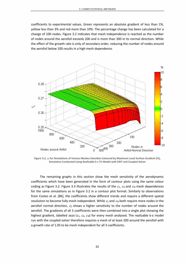
3. COMPUTATIONAL METHODS
coefficients to experimental values. Green represents an absolute gradient of less than 1%, yellow less than 3% and red more than 10%. The percentage change has been calculated for a change of 100 nodes. Figure 3.2 indicates that mesh independence is reached as the number of nodes around the aerofoil exceeds 200 and is more than 300 in its normal direction. While the effect of the growth rate is only of secondary order, reducing the number of nodes around the aerofoil below 100 results in a high mesh dependence.
Figure 3.2, cL for Simulations of Various Meshes Densities Coloured by Maximum Local Surface Gradient (%), Simulation Conducted Using Realizable k-ɛ TU Model with EWT and Coupled Solver
The remaining graphs in this section show the mesh sensitivity of the aerodynamic coefficients which have been generated in the form of contour plots using the same colour coding as Figure 3.2. Figure 3.3 illustrates the results of the cL, cD and cM mesh dependences for the same simulations as in Figure 3.2 in a contour plot format. Similarly to observations from Costes et al. [86], the coefficients show different trends and require a different spatial resolution to become fully mesh independent. While cL and cM both require more nodes in the aerofoil normal direction, cD shows a higher sensitivity to the number of nodes around the aerofoil. The gradients of all 3 coefficients were then combined into a single plot showing the highest gradient, labelled max (cL, cD, cM) for every mesh analysed. The realizable k-ε model run with the coupled solver therefore requires a mesh of at least 200 around the aerofoil with a growth rate of 1.05 to be mesh independent for all 3 coefficients.
62

3. COMPUTATIONAL METHODS
Figure 3.3, Top: Individual cL, cD and cM Performance, Bottom: Combined Mesh-Independent Region max (cL, cD, cM), Simulations Conducted Using Realizable k-ɛ Model, EWT and Coupled Solver
Re-running the simulations using the standard and RNG k-ɛ models confirmed that increasing the number of nodes around the aerofoil while decreasing the growth rate yields a mesh independent solution for the coupled solver, as seen on the left of Figure 3.4 for the standard k- ɛ model. The segregated solvers however show a different behaviour in that a very low growth rate causes cL and cM to change significantly, making it impossible to obtain a truly mesh independent solution with a single simulation for the aerofoil and wind conditions examined. This trend has also been observed when analysing different k-ɛ models, although it has been observed to a lesser degree than with the standard k-ɛ model which is shown in Figure 3.4. As a result the coupled solver has been used throughout this thesis.
The full set of simulation results for the standard k-ε model run with the SIMPLE, PISO and coupled solver and the k-ε RNG model run with the SIMPLE and coupled solver is shown in the appendix in section 9.3.1and 9.3.2 respectively in the form of contour plots for cL, cD, cM and max (cL, cD, cM).
63

3. COMPUTATIONAL METHODS
Figure 3.4, Comparison of the Coupled and SIMPLE Solver, Simulations Conducted Using Standard k-ɛ Model with EWT
Turbulence Model Study
The purpose of this study is two-fold: Various TU models from the S-A, k-ε and k-ω model families have been analysed, both with respect to their grid sensitivity and their ability to accurately reproduce experimental cL, cD and cM. Grid sensitivity plays a significant role as full wind turbine meshes may have to trade complete mesh independence in the favour of a shorter computational time and therefore benefit from the use of robust TU models.
Figure 3.5 shows the percentage error of the aerodynamic coefficients produced by all TU models tested for the NACA 654-421 aerofoil, relative to the experimental values obtained by Devinant et al. [45]. Devinant et al. measured a cL, cD and cM performance of 0.292, -0.056 and 0.013 respectively at a Re of 400,000, a turbulence intensity of 4% and α of 0°. The force balance used for the measurements resulted in an uncertainty of ± 3-5% for cL and cM. Solutions from mesh independent or near mesh independent grids have been selected for the comparison. While all TU models had the tendency to overestimate cD which may be related to difficulties in accurately determining cD experimentally, cL and cM predictions showed lower errors. Particular emphasis has been given to cM as the coefficient assesses the underlying
64

3. COMPUTATIONAL METHODS
pressure distribution around the aerofoil rather than just the magnitude of the resolved pressure forces as reflected in cL and cD.
Figure 3.5, Accuracy of cL, cD and cM Prediction for S-A, k-ε and k-ω TU Models for the NACA 654-421 Operating at Re = 400,000 and α = 0°
The k-ε TU model family used in conjunction with the EWT has consistently delivered the most accurate cL prediction although it produced a considerable cM error of ≈ 30%. Using the same model with the SWF increased the cD and cL error but resulted in a reduction of the cM error. However when using the SWF, Eça and Hoekstra [73] found that the assumptions made when using a wall function approach are often not satisfied, even for a simple 2D flow over a flat plate. Their study showed that the flow inside the viscous sub-layer was predicted accurately when using a wall function approach, but the flow in the log-law region is not only TU model dependent but also Re dependent. For this reason the k-ε SWF has not been considered for wind turbine simulations where the accurate simulation of flow separation for a wide range of Re is crucial. Compared to the k-ε EWF, the k-ω model has simulated cM very accurately, particularly the k-ω SST model has delivered superior performance. The k-ω SST model also predicts the most accurate cD, although the under-prediction of cL is slightly increased. Finally, the S-A model shows a very inconsistent prediction of all 3 coefficients. When using the model with a fine near wall mesh, cD is highly over-predicted and cL is under-predicted. It performs better when using a coarse near wall mesh, but still produces considerable errors. Following is a discussion about each model’s mesh sensitivity and its capability of consistently predicting aerodynamic coefficients even when using a relatively coarse mesh.
65

3. COMPUTATIONAL METHODS
When refining a grid around an aerofoil, Costes et al. [86] found that different regions of their aerofoil produce different responses. While some regions experienced an increase in pressure others experienced a decrease. This can result in complex, non-monotonic convergence behaviour. Gleize et al. [75] investigated the grid convergence behaviour of different TU models using the same aerofoil. Their studies indicated that high gradients of μT are responsible for high mesh density requirements. This is in agreement with the results of the present grid sensitivity study where great variations in the grid sensitivity between different TU models and near wall treatments have been observed, as shown Figure 3.6 which illustrates max (cL, cD, cM) for all investigated models. The individual cL, cD and cM performances of all examined TU models are additionally illustrated in the appendix in section 9.3.3 through 9.3.6. The analysis yielded similar grid sensitivity patterns within each TU model family due to consistent method of computing μT within each TU model family. Gleize et al. [75] further observed particularly high gradients of μT at the outer edge of the BL which explains the high influence of the near wall treatment for the S-A and k-ε model observed in this study. The computation of ε for wall adjacent cells for instance differs significantly between the SWF and EWT approach [74].
In this study, all of the models tested showed high mesh dependence when the number of nodes around the aerofoil dropped below 100 – 200. Above that range the models were only sensitive to the applied growth rate. This is in agreement with observations made by Gleize et al. [75]. Their TU model comparison showed that outside the mesh independent region, the S-A model is more sensitive to the mesh than the k-ω model. Independent studies investigating the flow over a flat plate by Eça and Hoekstra [73] have shown that this is caused by a higher numerical uncertainty of the S-A model than the k-ω model when predicting BL flow. These shortcomings of the S-A model are reflected in the rapid gradient changes, both with a fine and coarse near wall mesh configuration, as shown in Figure 3.6. Enabling low Re-damping for the fine mesh did not alter the results.
In the present study the k-ω models have shown a more consistent gradient evolution for a range of meshes than the S-A model. The observed non-monotonous convergence behaviour of the k-ω model has also been reported by Gleize et al. [75] for the SST model. In this study the generation of a truly mesh independent grid was limited by cL and even more so by cM as it can be seen in Figure 9.8. Growth rates of up to 1.15 are acceptable for the simulation of near mesh independent aerodynamic coefficients. Gleize et al. [75] recommend a mesh resolution of around 130 nodes in the BL in the aerofoil normal direction for attached flow and around 260 nodes for stalled flow when using the Wilcox k-ω model, this however is not feasible given the prospect of simulating an entire wind turbine.
The mesh sensitivity of the k-ε models has also been shown to be dependent on the near wall treatment. When used in conjunction with the SWF, more nodes around the aerofoil are required than when used with the EWT. It is also more sensitive to the growth rate. From all k-ɛ models tested with the EWT, the RNG model is particularly tolerant to meshes with a large growth rates. A growth rate of up to 1.1 results in mesh independent aerodynamic coefficients and growth rates of up to 1.25 are acceptable for only mild mesh dependences.
66

3. COMPUTATIONAL METHODS
Figure 3.6, Mesh Sensitivity of the max(cL, cD, cM) Parameter for S-A, k-ε and k-ω TU Model Families Simulating a NACA 654-421 Aerofoil Operating at Re = 400,000 and α = 0°
67

3. COMPUTATIONAL METHODS
Based on this analysis the choice of suitable TU models was narrowed down to the RNG k-ε model with the EWT and the SST k-ω model with and without low Re corrections. While the k-ω SST model offered a lower error in predicting cM and cD, the k-ε RNG model predicted higher aerodynamic coefficients but has been shown to be by far the most mesh insensitive TU model. Therefore those models were carried forward for further analysis in subsequent sections in order to evaluate the TU model best suited to turbine simulations.
3.2.3 Flow Field
The k-ε RNG and k-ω SST model with and without low Re correction have been examined for their capability of accurately simulating the flow field around an aerofoil using experimental data from Fujisawa et al. [90] and Sicot et al. [91]. The TU models were tested using an O-mesh with 320 nodes around the aerofoil and a growth rate of 1.06. The following studies have been conducted:
Boundary Layer Characteristics Wake Structure
Boundary Layer Characteristics
Experimental data derived by Fujisawa et al. [90] has been used in this section. They measured the skin friction, cf, around a NACA 0018 aerofoil using Particle Image Velocimetry (PIV) and a liquid crystal method. The aerofoil operated at α of 0 and 6° and was subjected to a chord Re of 80,000 and a turbulence intensity of 1%. Both experimental techniques gave similar results. They also recorded the velocity and turbulence intensity field around the aerofoil.
Figure 3.7 shows the comparison of cf simulated by the TU models and the experimental data at α 0 and 6°. As a reference, cf generated by a laminar simulation has also been shown between the LE and c = 0.2. None of the TU tested models predicted cf or the flow separation and reattachment correctly for both α’s. Skin friction has been shown to be much more sensitive to the type of TU model used, i.e. fully turbulent or transitional model, than the previously investigated pressure forces [93]. This is a consequence of the higher momentum within a turbulent BL than a laminar one which can only be resolved correctly by transitional turbulence models, not but fully turbulent ones. This has been described in detail at the end of section 2.6.1 where the limitations of full turbulent TU models are discussed. Numerical difficulties in predicting flow separation that occurs relatively far downstream from the LE also contribute to inaccurately simulated flow separation as numerical errors accumulate inside the BL and are transported downstream [86]. Furthermore cf has been shown to be highly sensitive to the mesh resolution, although when the mesh is within the grid independent region, the uncertainty of cf is very low [73].
68

3. COMPUTATIONAL METHODS
Figure 3.7, Validation of the Suction Surface Shear Stress of the NACA 0018 Using k-ε and k-ω TU Models [90]
Figure 3.8 and Figure 3.9 show the velocity and turbulence intensity contours respectively, measured at the same flow conditions as in Figure 3.7. The k-ε RNG model fails to predict any experimentally observed flow separation and does not accurately capture the trends of cf or the turbulence intensity field for both α, merely the velocity field follows experimental trends upstream experimentally observed separation points.
The k-ω SST models are in better agreement with the experimental data. Both models mimic laminar flow at the aerofoil’s LE. Enabling the low Re correction improves the prediction of cf at α = 0° and causes the formation of a separation bubble between 0.53 < c < 0.78 which is in close agreement to experimental separation bubble at 0.5 < c < 0.82, but the simulated bubble is too thin. When α = 6° cf on the suction surface is over-predicted at the LE and no experimentally observed separation on either blade surface is simulated.
Running the model without the low Re correction term improves the prediction of the turbulence intensity field and velocity field but fails to predict a separation bubble at α = 0°. The over-prediction of cf from c ≈ 0.3 is responsible for this. At α = 6° the model predicts a lower cf which is in closer agreement with experimental data at the LE. Although the experimentally observed separation bubble at 0.2 < c < 0.53 has not been captured, a TE flow separation on the aerofoil’s suction surface from c ≈ 0.81 has been simulated. The under-prediction of the flow separation of the k-ω SST model has also been reported in literature [86]. No TU model predicted the flow separation from c = 0.7 on the Pressure Surface (PS) of the aerofoil when α = 6°.
69

3. COMPUTATIONAL METHODS
Figure 3.8, Validation of Velocity Field of the NACA 0018, S = Separation, R = Reattachment (Experiment [90])
Figure 3.9, Validation of the Turbulence Intensity Field of the NACA 0018, S = Separation, R = Reattachment [90]
70

3. COMPUTATIONAL METHODS
Wake Structure
The wake of the aerofoil has been compared with PIV measurements from Sicot et al. [91]. They measured the vorticity field of the NACA 654-21 as it operated at a Re of 140,000 and α of 37°. The comparison of the vorticity field predictions of the TU models against the experimental data is illustrated in Figure 3.10.
All TU models predicted the vorticity produced by the LE and TE flow separation relatively well, although they have the tendency to produce slightly wider paths than those recorded in the experiment. The shed vorticity of the k-ω SST models is slightly wider than that of the k-ε RNG model. Enabling the low Re correction of the k-ω SST model did not result in any noticeable difference.
Figure 3.10, Validation of the Vorticity Field of the NACA 654-21 [91]
In conclusion the k-ε RNG model had the most difficulties in accurately predicting the boundary layer flow characteristics which are of great importance for this dissertation. It has therefore been omitted from further analysis. Enabling the low Re correction term of the k-ω SST model only partly resulted in improved boundary layer predictions which were limited to very low α. As a result of these studies, the k-ω SST model without low Re correction was chosen for all further studies investigating the flow around wind turbines.
71

3. COMPUTATIONAL METHODS
3.3 Wind Turbine Simulation Validation and Verification
This section aims at establishing an accurate method of simulating starting sequences of wind turbines. Due to the large number of sequences analysed in the results chapters it was important that the chosen method only requires a minimum computational time. Depending on the turbine scale and wind speed, a starting sequence can take up to 130 flow seconds which at a time step size of 10-3s results in 130,000 time steps for a single starting sequence. The majority of the computations were run on the University of Sheffield’s HPC cluster Iceberg. From the available CPU’s Intel Westmere based nodes were predominantly used. Each node has 12 cores and a total memory of 24GB RAM. The Iceberg HPC cluster allowed a maximum of 48 cores to be used for parallel computations. Although not always possible, most transient wind turbine simulations were run with 48 cores. With the available computational power and the indicated time step size, a single time step required on average 2 minutes and thus results in a computational time of up to 180 days.
Physical BC’s Mesh Pressure-Velocity
TU Model Temporal
Discretisation
Residual Convergence
Criteria Validation
R = 5.029m λ = 1.5-5.4
(Section 3.3.2)
Boundary Layer
Analysis Coupled k-ω SST
Steady & 10-2 – 10-4s
10-3 – 10-5 Torque & Pressure
Force [35] R = 0.3 & 0.6m λ = 1.5-6.5
(Section 3.3.2) Hybrid Coupled k-ω SST Steady 10-4 Torque [67]
R = 5.029m λ = 0.5- λDesign (Section3.3.3)
Hybrid Coupled k-ω SST 10-2 – 10-3s 10-4 Starting Torque
Table 3.2, Verification and Validation Process of the NREL Phase VI Wind Turbine Simulations, Fields with Multiple Entries have been the Focus of Respective Studies
Initially wind turbine simulations with a constant rotational speed were verified and validated, then a time-accurate starting sequence was simulated which was then compared to a less computationally expensive quasi-steady method of generating starting sequences. Finally the accuracy of the chosen computational method has been assessed. For all simulations the k-ω SST model, which has been identified as the most suitable TU model in the previous chapter, has been used. An overview of the wind turbine simulations conducted is in this section is provided in Table 3.2.
The convergence of each simulation has been ensured by computing the residual convergence and checking for torque periodicity. For transient simulations the torque convergence within a time was also checked. To aid the convergence of wind turbine simulations and assist simulation stability, only the lowest λ simulations were initialised; the
72

3. COMPUTATIONAL METHODS
converged flow solution was then used as an initial solution for higher λ simulations. Transient sliding mesh simulations also used MRF flow solutions of the corresponding λ as initial guess as it is shown in Figure 3.11. Such convergence techniques have also been used in literature [94].
Figure 3.11, Order of Wind Turbine Simulations to Aid Convergence, Simulation Stability and Reduce Simulation Time
3.3.1 Spatial Discretisation
The mesh topology and boundary conditions used throughout this chapter are shown in Figure 3.12 and Figure 3.13. Based on the findings in section 2.6.3 a hybrid gird with a similar topology to that of Mahu and Popescus [61], has been adopted for all wind turbine simulations in this research due to its high cell-efficiency while producing accurate simulation results. Figure 3.12 shows the topology of the mesh for the NREL Phase VI blade used for this dissertation. Due to the symmetry of the turbine and inflow conditions considered in this thesis, only a 180° sector containing 1 blade of the 2 bladed turbine was modelled. The surface of the blade is covered with a fully structured grid which is extruded to form the structured boundary layer block, labelled as Block 1. Block 1 is surrounded by an unstructured block, Block 2, to reduce the mesh size of the far-field. The far-field is composed of Block 3 and 4 which are separated by a circular interface at 1.5R to allow for a sliding mesh simulation. More details on how the mesh was generated can be found in the appendix in section 9.1. The turbine nacelle was not covered by a fine BL mesh. Ameur and Masson [76] found that the increase in computational cost when resolving the near wall flow at the nacelle does not justify the slight improvement of the results.
73

3. COMPUTATIONAL METHODS
Figure 3.12, Topology of Wind Turbine Mesh for the NREL Phase VI Blade
The cell zone conditions of each block when using different simulation strategies are summarised in Table 3.3. In Moving Reference Frame (MRF) simulations all blocks are fixed in space while in the sliding mesh configuration only block 4 is stationary, block 1 to 3 are rotating. In simulations with variable rotational speed, a User Defined Function (UDF) is hooked to the rotating cell zones.
MRF Simulation Sliding Mesh Simulation Start-Up Simulation Block 1-3 MRF Rotating UDF Block 4 MRF Stationary Stationary
Table 3.3, Cell Zone Conditions for Different Simulation Methods in Fluent Corresponding to Figure 3.12
The boundary conditions of the mesh and the mesh extent are illustrated in Figure 3.13. A broad range of mesh dimensions was found in literature with small meshes only measuring 2, 2.4 and 4R [63] and large ones extending up to 10, 10 and 20R [95] in the radial, upwind and downwind direction respectively. In this research external dimensions of 4, 5 and 6R in the upwind, radial and downwind direction respectively were chosen to avoid interference of the far-field boundaries with the flow around the blade while not creating an unnecessarily large mesh.
74

3. COMPUTATIONAL METHODS
Figure 3.13, Boundary Conditions and Domain Extent of the NREL Phase VI Blade
3.3.2 Constant Rotational Speed Performance
Basic computational schemes have been verified in this section to ensure the accuracy of the wind turbine simulation in this thesis and turbine performances at different scales have been validated. In order to allow for the evaluation of a time-accurate transient starting sequence in the next section, both the steady and transient solvers were studied. The following studies were investigated in this section:
Mesh Independence Study Turbine Scale Study Convergence Criteria for Transient Solver Time Step Size Study
The full scale NREL Phase VI rotor which has a radius of 5.029m has been used for verification and validation purposes in this section. The Turbine Scale Study additionally validated the computational methods at a 12 and 6% rotor scale. This study was conducted to ensure an accurate simulation of the 5.029m radius and the 0.334m radius rotor analysed in chapter 4, 5 and 6. The performance data for the full scale NREL Phase VI turbine has been simulated over a wind speed range of 7 to 25.1m/s which at a rotational speed of 72rpm corresponds to a λ range of 5.4 to 1.5 respectively. When investigating the smaller rotors, the rotational speed has been adjusted accordingly to match vw and λ. The 12% rotor thus rotated at 600rpm and the 6% machine rotated at 1,200rpm. All 3 scales were analysed using an identical pitch configuration of 3° between the rotational plane and the blade tip chord line.
Detailed experimental measurements of turbine torque and static pressure around the blade were collected in the NREL laboratory for the full scale machine [35]. For the 12% scale rotor only the turbine torque has been measured at the Korea Aerospace Research Institute (KARI) at a turbulence intensity of less than 0.1% [96]. Turbine blades with a radius of 0.334m,
75

3. COMPUTATIONAL METHODS
which corresponds to a 6.64% scale, have been manufactured to measure the turbine torque in the wind tunnel at the University of Sheffield. The experiments however could not proceed as planned due to unforeseen problems with the measuring equipment.
Mesh Independence Study
The experimental data of the full scale NREL Phase VI turbine was chosen for the validation of the generated grids, as this data provided the most detailed measurements. Four meshes ranging from 4.2 to 12.6 x 10⁶ cells were generated in this study. The distribution of cells in each mesh and the boundary layer properties are stated in Table 3.4 and Table 3.5 respectively. More details on the simulation settings of this study can be found in Table 3.1. This study has been conducted using the steady solver.
Mesh Total Boundary Layer Block 1
Transition Block 2 and 3
Far-Field Block 4
Very Coarse 4.2 0.6 0.6 3.0 Coarse 5.2 1.3 0.9 3.0 Medium 6.2 2.6 1.6 3.0 Fine 12.6 6.9 2.7 3.0
Table 3.4, Cell Counts x 106 of a 180° Mesh Section Modelling a Single Turbine Blade as Shown in Figure 3.13
Mesh Nodes Span Wise Nodes Chord Wise Growth Rate Very Coarse 84 58 1.1 increasing to 1.2 Coarse 115 88 1.1 increasing to 1.2 Medium 161 124 1.1 increasing to 1.2 Fine 227 180 1.1
Table 3.5, Description of Boundary Layer Mesh Characteristics of Block 1 in Figure 3.13
The resulting normalised pressures along the blade at r/R = 0.3, 0.47, 0.63, 0.8 and 0.95 for λ = 1.5, 1.9, 2.5, 3.8 and 5.4 are presented in Figure 3.14 along with experimental measurements and their corresponding standard deviations. The experimentally measured pressure has been observed to show an increased level of fluctuation when the flow is on the verge of undergoing significant changes such as flow transition or partial flow separation [35]. These regions showed a correlation with inaccurately simulated pressures and/or grid sensitive regions on the blade. Following this is an analysis of the mesh size requirement to accurately simulate the blade surface pressures of NREL Phase VI blade along with an analysis investigating the cause of any deviations between computations and experiments.
76

3. COMPUTATIONAL METHODS
An excellent match with experimental data has been observed when the flow around the blade is fully attached at high λ. At λ = 5.4 the majority of the flow is attached to the blade which eliminated any mesh dependence of the tested grids as no complex flow features have to be resolved.
When decreasing λ, the blade has been observed experimentally to operate under partially stalled flow conditions with a significant increase of the cpr fluctuations on the inner half of the suction surface. At λ = 3.8 a slight mesh dependence is observed for a large section of the suction surface. While the flow is predicted correctly along the majority of the blade, there is no indication that further mesh refinement would improve the inaccurately simulated flow at r/R = 0.47. The mismatch could be the result of an incorrectly simulated boundary layer as the k-ω model has the tendency to under-predict flow separation as shown in section 3.2.3. The flow around the experimental blade may have become stalled at that section as a consequence of the formation of a laminar BL which has not been able to withstand the adverse pressure gradient. The simulated BL however has a rather turbulent nature due to the use of a fully turbulent TU model as described in section 2.6.1. The increase in momentum thus allowed the flow to remain attached. Findings by Ekaterinaris and Menter [66] also suggest that the simulation error is a consequence of the limitations of the TU model used. When using a fully turbulent TU model for the simulation of flow around an aerofoil, they also observed the formation of a sharp suction peak which has not been observed when using a transitional TU model. The investigation of transition TU models however was outside the scope of this project. When λ further decreased to 2.5, a strong mesh dependence was observed. The ‘Very Coarse’ mesh wrongly predicts separated flow at the blade tip and yields a sharp suction peak at the root. All other meshes give relatively similar results for the majority of the blade. However a mild mesh dependence has been observed at r/R = 0.8. All grids slightly over-predict the rate at which the suction peak at the blade tip decays when moving radially inwards. Furthermore the grids fail to accurately predict the flow at r/R = 0.3, which could have a similar cause to the incorrectly predicted flow at r/R = 0.47 when λ = 3.8. Other researchers experienced similar problems in matching the experimental cpr near the blade root at low λ [61, 62, 64].
When λ drops below 1.9, the majority of the blade experiences fully stalled flow. Although a very sharp suction peak has been simulated along the entire blade span, the simulated results agree well with the experiment for r/R ≥ 0.47. The characteristics of the simulated BL at the leading edge did not affect the accuracy of the simulation for r/R ≥ 0.47 due to the high α at low λ which causes the flow to separate irrespective of its BL properties. The high blade twist at the blade root could be the cause of the over-prediction of the suction peak at r/R = 0.3 when λ = 1.9 as the resulting low α allows a turbulent BL to remain attached for longer than a laminar BL. The inaccurate simulation of cpr in that region however could also be the consequence of insufficiently resolved rotational effects, as the prediction of the simulation at the leading edge slightly improves with mesh refinement.
77

3. COMPUTATIONAL METHODS
Figure 3.14, Validation of cpr Performance of Meshes of Different Densities for the NREL Phase VI Rotor
78

3. COMPUTATIONAL METHODS
In conclusion, the mesh labelled ‘Very Coarse’ showed a high mesh dependence along the entire blade for λ = 2.5. The other meshes predicted relatively consistent results except for λ = 2.5 at r/R = 0.8 and λ = 1.5 - 1.9 at r/R = 0.3. The ‘Fine’ and ‘Medium’ meshes offered some improvement in the cpr prediction when λ = 1.5 and 1.9 near the root, but their benefit did not outweigh the cost of the computational time which was several times that of the ‘Coarse Mesh’. As a result the ‘Coarse Mesh’ had been used for all following simulations.
The overall findings that very low and very high λ have been simulated satisfactory as the majority of the flow is separated or attached at those conditions, corresponds to commonly observed trends in the literature [69]. Regions where the simulated cpr significantly deviated from the experimental values have been analysed in detail in Figure 3.15 using the ‘Coarse Mesh’. The role of these deviations on turbine acceleration which determines the rotor’s starting performance has been investigated in more detail in section 3.3.3.
Figure 3.15, Analysis of Radial Sections with Inaccurately Simulated cpr
The over-prediction of cpr at the leading edge of the suction surface at r/R = 0.3 when λ = 1.9 almost vanished when moving radially outwards to r/R = 0.34 and the under-prediction towards the trailing edge is also reduced, although not the same extent. The net effect of the inaccurately simulated cpr near the blade root on the turbine’s total torque at λ = 1.9 is therefore expected to be minor. When λ = 2.5 a better match to experimental data at the blade root is achieved between r/R = 0.38 and 0.42 than at the experimental measurement location of r/R = 0.3. The effect of the inaccurately simulated cpr is therefore expected to be slightly higher at λ = 2.5 than at 1.9. Only the cpr distribution at r/R = 0.47 when λ = 3.8 was found to not improve at all when moving radially inwards or outwards. This was expected based on the observation of a continuous suction peak along the blade span in Figure 3.14. The effect this has on the turbine torque is expected to be relatively low as the experiment only indicates a lack of the suction peak at r/R = 0.47 and the other radial locations have been simulated accurately.
79

3. COMPUTATIONAL METHODS
Turbine Scale Study
The torque of the NREL Phase VI turbine has been validated against experimental data from a full scale rotor and a 12% scale rotor. Additionally, the present simulation results of a 6% scale machine have been compared to computational results of Park et al. [67] as no experimental data has been available at this scale. To allow for a meaningful comparison at the 6% scale, the accuracy of Park et al.’s [67] simulation with respect to experimental data has first been assessed on the 12% turbine scale.
Figure 3.16, Torque Validation of a Single Blade of Full Scale NREL Phase VI Turbine Using the k-ω SST Model
Figure 3.16 shows the torque comparison of the full scale rotor along with computed standard deviations. The corresponding pressure distributions along various blade sections are illustrated in Figure 3.14. An excellent torque agreement between the simulations and the experimental values of the average torque at low λ has been achieved. Only λ = 5.4 shows a significant deviation, however as this λ is not of great relevance for a turbine’s starting behaviour, the mesh and computational settings used are deemed to be adequate.
The comparison between the present simulations and the experiments conducted in the KARI wind tunnel at a 12% scale are shown in Figure 3.17. Simulation results from Park et al. [67] at the same turbine scale have also been included for reference. The present simulations are observed to reproduce the experimental trends in the evaluated λ range. Compared to the full scale NREL turbine simulation, the 12% scale shows a higher deviation from experimental results which might be caused by larger parts of the blade experiencing laminar flow. Experimental inaccuracies, which could not be examined properly by the author of this thesis
80

3. COMPUTATIONAL METHODS
due to the limited availability of experimental documentation, could also be the cause for deviations. Nonetheless, a good match with the experiments has been achieved at low λ. In the range of 2.5 < λ < 3.8 a slight over-prediction of the turbine’s torque has been observed which is likely to be linked to the difficulty in accurately simulating partially stalled flow as observed previously for the full scale turbine. The observed experimental toque peak at λ ≈ 4.1 has been reduced in magnitude and is shifted towards a lower λ which suggests that the simulated flow attaches to the blade at a too low λ. For high λ, the simulation is observed to under-predict the turbine’s torque, following the trend of the full scale simulations.
Figure 3.17, Torque Validation of a Single Blade of 12% NREL Phase VI Turbine Using the k-ω SST Model and Comparison to Park et al. [67]
The simulations conducted by Park et al. also capture the experimental trends but their simulation significantly over-predicted the turbine’s torque when λ < 4. They observed a similar shift of their toque peak with respect to the experimental data to what has been observed in this research, but their torque peak at λ ≈ 3.4 is more pronounced.
Figure 3.18 shows the comparison of the simulations conducted by Park et al. at a 6% scale and those conducted in this research at the 6.64% scale. The offset between the simulations is very similar to that observed at the 12% scale in Figure 3.17 which suggests that the present simulations follow a correct torque trend. Discrepancies can furthermore be attributed to the small difference in the turbine scale and simulation inaccuracies.
81

3. COMPUTATIONAL METHODS
Figure 3.18, Torque Comparison of a Single Blade of 6% NREL Phase VI Turbine to Park et al. [67] Using the k-ω SST Model
Convergence Criteria for Transient Solver
This study and the remaining studies in this section verify the correct use of the transient solver using the full scale rotor. This is an essential step in the preparation for the transient wind turbine start-up simulation, as they are initiated from a converged sliding mesh simulation of a constant rotational speed solution as it is indicated in Figure 3.11.
The converged results of the steady solver have been used as an initial guess for the transient solver which was set to a time step size of dt = 10-3s. Three studies which terminated the iterations within a time step when the maximum residual fluctuation was less than 10-3, 10-4 and 10-5 were conducted. A maximum of 20 iterations per time step was allowed. A sample torque history at λ = 2.5 displaying the torque at each iteration of the steady solver and thereafter at the last iteration of each time step of the transient solver is shown in Figure 3.19 along with the experimental mean and standard deviation of the torque.
Near-torque independence of the transient solver is achieved when the residual convergence criteria is lowered to 10-4 at λ = 2.5. The change from the steady to the unsteady solver has slightly lowered the computed average torque but it still produces a good match with the experimental torque. The experimental standard deviation of 47Nm however has been under-predicted by 34.5Nm. Fluctuations of the simulated aerodynamic torque have also been observed in literature as a result of periodic separation and vortex shedding [68].
The same residual convergence requirement has been identified for λ in the range of 1.5 to 5.4. A convergence criterion of 10-4 has therefore been used for the remainder of this thesis to minimise the accumulation of inaccuracies between time steps but not spend too much
82

3. COMPUTATIONAL METHODS
time on computations. An accurate computation of the torque is essential to enable an exact simulation of a transient turbine start which can last for up to 130 flow-seconds.
Figure 3.19, Torque Convergence of Steady and Transient Solver, Convergence Criteria 10-3-10-5
Time Step Size Study
This study investigated the effect of time step sizes from 10-2s to 2.5 x 10⁻⁴s when the full scale turbine operated at λ = 2.5. To visualise the interaction between the convergence criteria of a time step and the required time step size, a detailed study illustrating the torque convergence within a time step is shown in Figure 3.20. The transient solver was run using 3 different time step sizes and corresponding levels of residual convergence have been indicated as the solver was allowed to compute 50 iterations. The torque of the suction and pressure surface as well as the total torque at iteration i has been normalised by the corresponding torque at the 50th iteration of each time step. Figure 3.20 shows that larger time steps require lower residual convergence criteria in order to reach torque convergence.
Figure 3.21 visualises the effect of the error carried forward between time steps for a range of time step sizes using a residual convergence criteria of 10-4s. A time step size of 10-3s along with a residual convergence criterion of 10-4 was deemed to be a good trade between accurately predicting the turbine torque and minimising computational time as this combination only incurred an error of 0.15% in the torque prediction per time step. The results of Figure 3.20 and Figure 3.21 are representative for a λ range from 1.5 to 5.4.
83

3. COMPUTATIONAL METHODS
Figure 3.20, Torque Convergence within a Time Step for Different Time Step Sizes, Corresponding Residual Convergences are Labelled in Boxes, R = 5.029m and λ = 2.5
Figure 3.21, Torque History at λ = 2.5 for Time Step Sizes Ranging From 10-2 to 2.5x10⁻⁴s
3.3.3 Transient Turbine Start-Up
This section uses the results of the previous studies in conjunction with a UDF in Fluent to simulate the starting behaviour of the NREL Phase VI machine using an inertia model. In order to efficiently, yet accurately, simulate a turbine starting sequence the following studies were conducted:
Torque Fluctuation at Low, Constant Rotational Speed Time Step Size Study
The structure of the UDF used for this research is illustrated in Figure 3.22. It is composed of 2 macros which are called at every time step to compute the turbine’s torque, convert it to a corresponding rotational speed using an inertia model and apply the updated rotational speed in the next time step. This process is repeated until the turbine has reached its full operational speed. The UDF has been programmed to regularly output the turbine’s
84

3. COMPUTATIONAL METHODS
rotational speed, the torque distribution along the blade as well as contours of the flow while the turbine accelerates to save disk space but not compromise on the availability of data for post-processing. Contours of the total torque and the rate of change of torque on the blade’s surface as well as velocity, pressure and vorticity fields in the near blade region were also exported during turbine starting. By doing so the required disk space for the turbine analysis was reduced by 99% from 1.0GB for a single case and data file to only approximately 10MB for all the post-processing data. This thus allowed the data to be exported every 10 time steps. The UDF also instructed Fluent to save a case and data file every 0.25 λ. The complete UDF can be viewed in the appendix in section 9.4, it is partly based on literature [97] but has been extensively modified and extended to suit the requirements of this dissertation.
Figure 3.22, Structure of UDF for a Transient Turbine Start-Up in Fluent
The start-up of the full scale and small scale NREL turbine was simulated at a constant wind speed of 6m/s. The full scale machine was modelled with an inertia of 949kgm2, the 6.64% scale machine had an inertia of 4.5 x 10⁻³kgm2. Both turbines were modelled with a zero resistive torque.
Torque Fluctuation at Low, Constant Rotational Speed
Prior to the start-up simulations a study investigating the magnitude of the torque fluctuations at very low λ was conducted to investigate the feasibility of initiating the start-up simulation from ω0 > 0rad/s in order to save computational time without compromising simulation accuracy. As can be seen in Figure 3.23 for the full scale rotor, periodic torque
Start: Converged Solution at ω0
𝑅𝑅𝑁𝑁+1 = 𝑅𝑅𝑁𝑁 +𝑇𝑇𝑁𝑁 𝑑𝑑𝑡𝑡𝐼𝐼
Update 𝑅𝑅𝑁𝑁+1 using DEFINE_ZONE_MOTION Macro:
𝑇𝑇𝑁𝑁 = 𝑇𝑇𝑃𝑃 + 𝑇𝑇𝑣𝑣𝑣𝑣𝑟𝑟
Calculate Torque using DEFINE_EXECUTE_AT_END Macro:
Output Data using DEFINE_EXECUTE_AT_END
Macro
Run Single Time Step
End: λDesign
85

3. COMPUTATIONAL METHODS
fluctuations in time only occur for λ > 0.5. The transient start-up simulations were therefore initiated from a converged flow solution at λ = 0.5. For the full scale NREL Phase VI rotor it takes 8.3 flow-seconds to reach λ = 0.5 from rest. Depending on the chosen time step size, it can take up to 12 days to simulate the starting sequence from λ = 0 to 0.4. The small scale machine follows a similar trend.
Figure 3.23, Torque Fluctuations for λ = 0 – 1.5 at Constant ω for Full Scale NREL Phase VI Rotor
Time Step Size Study
The NREL Phase VI turbine has previously been observed to produce a fluctuating torque when operating at a constant rotational speed which is likely to be caused by vortex shedding. The acceleration of the turbine during a starting sequence in combination with the observed vortex shedding at constant rotational speed, might produce additional unsteady effects and therefore requires the evaluation of a suitable turbine starting dt.
When a turbine freely rotates it tends to accelerate rapidly after λ ≈ 3. The time step size study was therefore initiated from ω = 3.58rad/s which corresponds to λ = 3 for the full scale rotor. Time step sizes of 10-2s and 5 x 10⁻³s were tested. Smaller time step sizes were computationally too expensive as a start-up simulation from λ = 0.5 to λDesign with dt = 5 x 10⁻³s requires approximately 7,600 time steps which translates to approximately 11 days computational time. The results of the time step size study are shown in Figure 3.24 for a flow time of 7s as the rotor had reached its design λ at that point. The simulated starting sequences of both time step sizes follow the same overall trend but show some small cT fluctuations which are partially caused by the torque fluctuations at constant rotational speed when λ > 0.5. The higher accuracy gained from the smaller dt has been considered insignificant with respect to the additional computational time requirement. It has therefore been concluded that a dt of 10-2s is sufficient. The residual and torque convergences within a time step have also been verified analogously to section 3.3.2. For the starting sequences in Figure 3.24 the iterations within a time step required for residual convergence were observed to slightly increase with increasing λ, as the flow field undergoes more rapid changes at higher λ. The maximum number of iterations per time step of 20 has not been exceeded.
86

3. COMPUTATIONAL METHODS
Figure 3.24, Starting Sequence for the Full Scale NREL Phase VI Turbine from λ = 3.0 at a Time Step Size of 10-2s and 5 x 10⁻³s
3.3.4 Start-Up Methodology
In this section a suitable methodology for modelling a turbine start-up using CFD has been evaluated using the full scale NREL Phase VI turbine at a wind speed of 6m/s as a reference. The CFD method was based on the findings of the previous sections in this chapter and the method’s accuracy has been analysed. As there is no experimental turbine starting data available which has been derived under a controlled flow environment, frequently conducted BEM simulations for modelling turbine starting sequences have been used as a reference for the CFD start-up methods. This section therefore first derives a suitable BEM model for turbine starting. Some information on BEM turbine start-ups from literature is given in section 2.5. Following, two conceptually different approaches to model a turbine start-up using CFD have been compared. Hereby the role of unsteadiness and hence the necessity of running a fully transient CFD start-up simulation vs. modelling a ‘quasi-steady’ CFD start-up has been identified. After choosing the better suited CFD method for modelling HAWT start-up, its accuracy has been assessed. The two CFD methods investigated are:
• ‘Quasi-Steady’ Method: This method estimates a turbine’s start-up behaviour from a λ – cT reference curve obtained from CFD simulations run at constant rotational
87

3. COMPUTATIONAL METHODS
speeds in 0.5 λ increments at the wind speed of interest. An inertia model was used to relate the torque which has been interpolated from the reference curve to a change in rotational speed and advance in time as shown in Equation 2.12. This method is very time efficient as it only requires a series of constant rotational speed simulations, but it does not account for any unsteady effects and therefore has to be verified.
• Fully Transient Turbine Starting: In this approach Fluent uses the turbine torque to freely accelerate the blades. The method has been described in detail in section 3.3.3.
This section has therefore been divided in the following sub-sections:
Derivation of BEM Start-Up Comparison of Fully Transient Start-Up, Quasi-Steady Start-Up and BEM Start-Up Error Analysis of Chosen CFD Start-Up Methodology
Derivation of BEM Start-Up
The BEM code FAST has been used to identify any differences between lower order BEM methods and CFD methods for simulating turbine start-ups. FAST is an open-source programme which has been developed by NREL for the simulation of 2 and 3 bladed HAWTs. FAST stands for Fatigue, Aerodynamics, Structures and Turbulence. However as the CFD computations only accounted for rotor aerodynamics, all of FAST’s modules except for the aerodynamics module have been inactivated as far as this was possible. For the calculation of its aerodynamics FAST uses the subroutine set AeroDyn. In this thesis FAST version 7.02 and AeroDyn version 13 have been employed. As part of FAST’s download package, NREL provides a set of input files for the simulation of the NREL Phase VI rotor which is labelled ‘test10’. These input files have been modified in order to conduct WT simulations in 0.5 λ increments at 6m/s wind speed. The corresponding turbine start-up has then been derived according to the quasi-steady method described at the start of this section with a conservative time step size of 0.001s.
Comparison of Fully Transient Start-Up, Quasi-Steady Start-Up and BEM Start-Up
The results of the BEM method, the time step size study using the quasi-steady CFD method and the fully transient method, which started from λ = 0.5 as discussed in the previous section, are displayed in Figure 3.25. For the quasi-steady CFD method a time step size of 1.00s caused significant errors when T > 35s. A time step size of 0.01s resulted in a converged starting performance from rotation initiation to full operational speed. This dt has therefore been used for the CFD quasi-steady turbine starting predictions of the full scale rotor. An equivalent dt for the small scale rotor of 7 x 10⁻⁴s has been evaluated using Equation 3.1 which scales the permitted rate of change of λ in time according to the turbine radius.
𝛿𝛿𝜆𝜆𝛿𝛿𝑡𝑡
∝ 𝑅𝑅
Equation 3.1
88

3. COMPUTATIONAL METHODS
Figure 3.25, Turbine Start-Up of the NREL Phase VI Using a BEM Method, a Fully Transient CFD Simulation and a Quasi-Steady CFD Simulation with a Time Step Size Study, R = 5.029m, vw = 6m/s
The starting sequence generated using the BEM method has been observed to be in good agreement with that of the fully transient method for λ < 3.3. Above λ = 3.3 the BEM method predicts a significantly higher cT when using BEM than both CFD methods which causes the rotor to accelerate faster. However as the rotor experiences a sharper cT reduction after it has reached its maximum cT than when using CFD, the BEM start-up duration is nearly identical to that of the fully transient CFD method. These differences are consistent with the under-prediction of the CFD turbine torque compared to experimental values that has been observed for a turbine operating at constant rotational speed in Figure 3.16. Furthermore, the accuracy of BEM programmes is typically optimised for turbine operations near λDesign. BEM may therefore be used to predict turbine starting reasonably accurately under a controlled flow environment.
89

3. COMPUTATIONAL METHODS
The overall trends of the fully transient turbine starting method and the converged quasi-steady CFD method during turbine starting are in good agreement, although there are some slight differences of a maximum of ±0.0064 cT and ± 0.24 λ at any given time. These discrepancies are caused by the cT fluctuations of the constant rotational speed simulations as well as some mild unsteady effects due to the turbine acceleration of the fully transient simulation which have been ignored in the quasi-steady method.
Table 3.6 summarises the deviations of the turbine starting parameters which are of relevance for chapter 6, namely λDesign, the turbine starting time Ts and the maximum cp. Additionally the computational time requirement of all methods is given. Both quasi-steady methods have been compared with respect to the fully transient method. This reference was chosen as this thesis is concerned about investigating detailed flow structures and torque features and their consequence on the annual energy yield as outlined in section 1.5. BEM methods do not provide such flow information and are therefore not suitable when aiming to explore fundamental turbine aerodynamics. Except for the under-prediction of the maximum cP of the CFD methods compared to the BEM method, all parameters are in good agreement. For the quasi-steady CFD method the deviations of all 3 parameters are kept within a bound of ±1.5% with respect to the fully transient method. Furthermore, the time requirement for running the transient method was prohibitively high for a very little improvement of the solution accuracy. The method of choice for this thesis was therefore the quasi-steady CFD method. Its inaccuracy has been evaluated in more detail in the following section.
Computational Method Transient Start-Up
(dt = 10-2s) Quasi-Steady
CFD Quasi-Steady
BEM Computational Time 7 weeks 4 days 1 minute Deviation of Design λ Reference +1.2% +4.6% Deviation of Starting Time Reference +1.5% -0.9% Deviation of Maximum cP Reference -1.3% +30.7%
Table 3.6, Accuracy and Computational Time Requirement of Different Start-Up Methods
Error Analysis of Chosen CFD Start-Up Methodology
In section 3.3.2 some inaccuracies in the CFD computations when prediction partially stalled flow have been identified with respect to experimental data. However as the experimental data has been derived by investigating different wind speeds rather than investigating a constant wind speed but varying the rotational speed, a quasi-steady starting curve cannot be estimated using the experimental data. Instead, the computational inaccuracies have been quantified by estimating the difference of the computational and experimental rotor acceleration at distinct λ. The experimental data provided in Figure 3.16 has been used for this comparison. The result is shown in Figure 3.26. It can be seen that the error in the change of rotational speed per second induced by an inaccurately simulated torque is less than 2% when λ ≤ 3.8. This very low error ensures an accurate overall prediction
90

3. COMPUTATIONAL METHODS
of the turbine start-up behaviour in that λ range. As λ increases to 5.4 the under-prediction of the simulated torque causes a 28% under-prediction in the rotational speed increase per second. This however has a comparatively little effect on the turbine start-up prediction as the turbine undergoes a rapid acceleration when λ > 3.8 which only lasts for the last ≈ 4s of the ≈ 47s long total starting sequence. This is in relatively good agreement with the trends observed in Figure 3.25. Neglecting Re effects and accumulating the acceleration error shown in Figure 3.26 over the turbine starting sequence using the quasi-steady method results in a 6.9% under-prediction of the total turbine starting time.
Figure 3.26, Error of Rotational Speed between Experimentally and Computationally Evaluated Torques per Second
In the following analysis the effect of inaccurately modelled starting sequences on the energy yield has been evaluated. The analysis could not be done using experimental reference data due to the difference of experimental and computational Re ranges as well as a lack of experimental data at λDesign. Figure 3.27 shows the resulting percentage error of the energy produced for both CFD starting methods when the turbine is subjected to a wind speed of 6m/s for 60s. The relatively large error in the prediction of the energy yield of the quasi-steady method just after the turbine begins to rotate is solely caused by the difference of the predicted turbine starting time of 0.69s for both methods. As the turbine rotates for longer the error drops down exponentially tending towards the maximum cP error. After time 60s, the energy yield error has reduced to -6%. The approximately 12 fold increase in computational time when using the transient method rather than the quasi-steady CFD method however did not outweigh the gain in accuracy.
91

3. COMPUTATIONAL METHODS
Figure 3.27, Percentage Error of the Energy Yield Estimated using the Quasi-Steady CFD Method with Respect to the Fully Transient CFD Method for Full Scale WTRef Operating at 6m/s
3.4 Summary
In this chapter high fidelity HAWT simulations, capable of accurately simulating a rotor starting sequence, have been derived. A bottom-up approach has been used where the complexity of simulations has been progressively increased from static 2D aerofoils simulations to the simulation of freely rotating wind turbines using CFD. A comparison with BEM has been made where no suitable experimental data was available. Following is a brief summary of the results of the studies.
Aerofoil Studies
• The coupled solver is preferable over a segregated solver as the segregated solvers were found to have difficulties in delivering truly grid independent results for cL, cD and cM.
• The k-ω SST model most accurately predicted aerodynamic coefficients while the k-ε RNG model has been shown to be most tolerant to grid variations in its cL, cD and cM predictions. Other members of the k-ε and k-ω model families and the S-A model showed inferior performance.
• The k-ω SST model outperformed the k-ε RNG model when predicting the flow field around an aerofoil. Enabling the low Re correction of the k-ω SST model resulted in slight improvements for α = 0° which disappeared for higher α. The k-ω SST model
92

3. COMPUTATIONAL METHODS
without Re correction has therefore been the model of choice for the following wind turbine studies.
Wind Turbine Studies
• A hybrid mesh of 5.2 x 10⁶ cells with heavy cell clustering around the blade was shown to be sufficient to produce an excellent rotor torque match with experimental data at low to medium λ. Deviations in the static pressure distribution along the blade from experimental values were found in partially stalled flows. They are a likely consequence of the use of a fully turbulent turbulence model.
• The torque trend for scaled down machines followed the experimentally observed patterns and those simulated by other researchers.
• Turbine starting can be modelled using a computationally expensive approach in which the CFD solver advances the blade in time using an inertia model during a transient simulation or by employing a quasi-steady method that interpolates the starting sequence from constant rotational speed simulations run at distinct λ.
• Fully transient simulations were initiated from λ = 0.5, as turbines rotating at constant rotational speeds of λ ≤ 0.5 produce no torque fluctuations. To reduce the computational time and aid simulation stability, the simulation was first run using the steady MRF solver until converged and then switched to a transient sliding mesh simulation with a residual convergence criterion of 10-4 and a dt of 10-3s. When converged, the variable rotational speed was implemented through a User Defined Function.
• Both turbine starting methods gave nearly time step size independent starting sequences when dt = 10-2s. The error of the energy yield predicted using the quasi-steady method, is highest when the turbine just begins to produce energy. It exponentially drops down to less than 6% when the turbine has produced energy for more than 11s. The higher accuracy of the fully transient method with respect to the quasi-steady method however did not justify the 12 fold increase in computational time associated with the fully transient method. Turbine starting has therefore been modelled using the quasi-steady approach for the remainder of this thesis. The general inaccuracies introduced by difficulties in accurately predicting flow separation at some λ regardless of the chosen start-up method has been estimated to be less than 6.9%.
• A comparison between the CFD turbine start-ups and a BEM starting sequence generated using the program FAST in combination with the quasi-steady method, has shown that there is a good agreement between the different approaches when λ < 3.3. At higher λ BEM predicts a higher cT which leads to a higher design cP which follows experimental trends. The total turbine starting time however is nearly identical. BEM may therefore be used to predict turbine starting reasonably accurately under a controlled flow environment. However as it does not resolve the flow itself it cannot be used for investigating flow features.
93

4. AERODYNAMIC PERFORMANCE OF THE REFERENCE BLADE
4.1 Introduction
This chapter introduces the aerodynamic performance of the reference turbine. The performance of the reference blade serves as a benchmark for chapter 5 where different parameters of the turbine’s geometry have been modified. This chapter introduces the analysis principles while describing the performance of the reference turbine in detail. The detailed investigations in this chapter along with chapter 5 form the foundation for the turbine starting analysis in chapter 6.
The geometry of the reference rotor corresponds to the NREL phase VI turbine which has also been used for the computational validation of this thesis in chapter 3. The turbine has a radius of 5.029m, a blade thickness of 21% and operates at 0° pitch. After establishing its performance at the reference wind speed of 6m/s, an investigation of the effect of the Reynolds number was carried out by scaling the turbine down to a radius of 0.334m while maintaining a wind speed of 6m/s. Subsequently the effect of varying the wind speed from 3m/s to 20m/s at both turbine scales has been examined. This data set forms the reference for the chapter 5.
The performance of the reference turbine is discussed in terms of its overall power and torque coefficients, its radial torque distribution as well as the role of the suction and pressure surfaces for generating torque. The torque has been related to the flow structures around the wind turbine blade. The data presented throughout this chapter originates from distinct simulations run at tip speed ratio intervals of 0.5 from a tip speed ratio of 0 to 6.

4. AERODYNAMIC PERFORMANCE OF THE REFERENCE BLADE
4.2 Reference Flow Condition
The full scale NREL Phase VI turbine has been investigated for λ ranging from 0 to 6 at a constant wind speed of 6m/s. The first half of this section discusses the power and torque performance of the turbine. The torque production of the blade is presented with an increasing level of detail to build an understanding of the parameters affecting the turbine’s performance. Initially an overview of the torque performance of the entire blade is given which is followed by an analysis of the radial torque distribution. Finally, an analysis of the contribution of the pressure and suction surface towards the total blade torque along with the torque distribution on both surfaces is presented. To the author’s knowledge, this type of analysis has not been presented in literature before.
The second part of this section visualises the flow around the turbine blade at selected operating conditions to relate the torque formation along the blade to the flow structure and consequently the turbine’s geometry. This analysis procedure served as a template for the investigation of different blade designs in chapter 5.
4.2.1 Power and Torque
The power and torque coefficients of the NREL Phase VI turbine are presented in Figure 4.1. The power output of the turbine continuously increases from cP = 0 at λRef = 0 until it reaches its optimum of cP = 0.26 at λRef = 5.5. The torque coefficient in contrast starts from 0.0075 at λRef = 0, peaks at cT = 0.054 when λRef = 4.3 and decreases to cT = 0.048 at λRef = 5.5. To gain a better understanding of the λ - torque distribution presented in Figure 4.1, thorough studies investigating the source of the torque have been conducted analysing:
Radial Torque Distribution Blade Surface Torque
Figure 4.1, Power and Torque Performance of the WTRef at 6m/s
95

4. AERODYNAMIC PERFORMANCE OF THE REFERENCE BLADE
Radial Torque Distribution
For a detailed torque analysis, the torque has been computed by discretising the blade into 50 uniformly spaced sections along its radius and summing the pressure and viscous torque produced at each cell that fall within a given radial section. It is worthwhile noting that a positive pressure distribution on the blade surface can either produce positive or negative torque, depending on its exact location with respect to the point where the local blade surface curvature is aligned with the plane of rotation. This is illustrated in Figure 4.2. For illustration purposes a positive pressure has been assumed to act around the entire S809 profile. The net pressure acts perpendicular to the local blade surface curvature whereas resulting pressure components used for torque calculation act in the plane of rotation.
Figure 4.2, Schematics of Pressure to Torque Translation
A detailed analysis of the torque produced along the blade span for λ = 0 to 6 is presented in Figure 4.3. Positive torque which can either act to accelerate the blade or produce power has been represented blue, radial locations producing no torque are white and negative torque is red. The absolute value of the positive and negative torque has been kept identical for a more intuitive interpretation of the resulting radial torque distribution. The observed stripes in the spanwise torque distribution in Figure 4.3 are caused by the alignment of individual blade surface cells, in which the torque is calculated, with a Cartesian coordinate system, whereas the torque of individual radial sections has been summed using a cylindrical coordinate system. The pronounced stripy appearance of the graph is therefore not physical but torque trends are indicated correctly.
The superposition of the geometrical α and Re on the torque contours of Figure 4.3 indicates that the majority of the power producing torque is generated by the upper half of the blade when α falls below 22°. This first occurs at the blade tip when λ = 2.5. Re only appears to be of secondary effect for the power producing torque. Normalising the torque of each radial section by the total torque produced at that λ, shows that the radially outwards increasing α at λRef = 0, in combination with the radially outwards decreasing Re, causes the torque of the NREL Phase VI turbine to be relatively uniformly distributed. When the rotational speed increases to 1 < λRef < 2.5, the majority of the starting torque is produced near r/R = 0.3.
96

4. AERODYNAMIC PERFORMANCE OF THE REFERENCE BLADE
Wright and Wood [48] observed that the torque produced at the tip of their turbine overtook the torque generated by the blade root in the range of 1.3 < λRef < 1.6, depending on the wind speed the turbine was subjected to. Their lower λ can be explained by the different chord and twist distribution along the blade compared to the NREL Phase VI turbine. As the NREL Phase VI rotor starts to rotate from λRef = 0, the rotational velocity component at the blade tip increases at a higher rate than at the blade root, which leads to a higher increase of Re at the tip than at the root. At λRef = 1.97 the effect of vrot favouring a high Re at the tip and the linear chord distribution of the blade favouring a high Re at the root, balances to produce an almost uniform Re distribution along the NREL Phase VI blade which only varies between 322,000 and 356,000, making the torque production predominantly a function of α. The significantly lower α at the blade root when λRef ≈ 2 then causes the majority of the torque to be generated between 0.27 < r/R < 0.34. Blade sections operating at α as high as 60° are shown to contribute to the starting torque at the root for a blade operating at very low λRef. This phase of the significant torque production at the root ends when α at the blade tip falls below 22° at λRef = 2.5 which allows the blade tip to generate a large torque. As λRef increases, the section of the blade operating at α < 22° also increases, which causes the rapid increase in cT seen in Figure 4.1 for 2.5 < λ < 3.5. When λRef > 4 the entire power producing upper half of the blade operates with α < 22° which leads to a relatively uniform torque production along the blade thereafter. The cause for the drop in cT as λ > 4.3 is discussed in the following analysis of the torque distribution on the blade surface.
Figure 4.3, Absolute and Normalised Torque of WTRef for λ = 0 - 6 with Geometric α and Re Superimposed
97

4. AERODYNAMIC PERFORMANCE OF THE REFERENCE BLADE
Blade Surface Torque
In this thesis a novel approach to quantify the effect of the pressure and viscous force on the torque performance of the blade has been employed. Figure 4.4 illustrates how the local blade curvature and blade radius interact with the static pressure to produce the pressure torque. The analysis is based on the same principles as outlined in Figure 4.2. Favourable regions of the blade producing positive torque and blade areas acting to reduce the total torque have been identified by plotting the fraction of the torque contribution of cell i, Ti, towards the total torque produced by the blade at a specific λ. The torque fraction has then been normalised with the corresponding cell area to remove the mesh dependence of the parameter as shown in Equation 4.1. Thus critical regions of the blade for the torque generation can be identified and more conclusions can be drawn from the analysis than from the pressure distributions alone which are commonly presented in literature [61, 79].
𝑇𝑇𝐴𝐴(𝑣𝑣) =𝑇𝑇𝑣𝑣
𝑇𝑇𝑎𝑎𝑛𝑛𝑟𝑟𝑜𝑜 𝐴𝐴𝑣𝑣� Equation 4.1
Figure 4.4, Effect of Static Pressure, Blade Curvature and Radius on Pressure Torque per Unit Area of WTRef at λ = 0
98

4. AERODYNAMIC PERFORMANCE OF THE REFERENCE BLADE
The local curvature of the blade in the chord-wise direction influences both, the magnitude and directionality of the pressure force on the local blade surface torque. When the tangent of the curvature of the blade is aligned with the rotational plane, the torque performance is independent of the pressure on the blade’s surface. This ‘zero-blade-curvature’ line is marked in Figure 4.4 as the black line running radially up the span. Its importance on the blade torque can be seen on the torque per unit area contour. Although the majority of the pressure surface experiences a positive pressure at λ = 0, only the area between the zero-blade-curvature line and the trailing edge produce a positive torque. The blade curvature acts to translate the positive pressure between the leading edge and the zero-blade-curvature line into a negative torque. The zero-blade-curvature line on the suction surface is shifted towards the trailing edge and touches it at r/R ≈ 0.3. A negative pressure at the leading edge and the blade root of the suction surface therefore translates to a positive torque, as can be seen in Figure 4.4. The torque results for the full turbine operating range are presented in Figure 4.5. While the torque pattern of the suction surface follows that of the blade curvature for all λ, the torque pattern on pressure surface is more complex.
Figure 4.5 presents data from the analysis of the contribution of the pressure and suction surface to the total torque and the torque’s origin on the blade surfaces over the full range of λ. When the turbine is stationary, it produces a torque coefficient of cT = 0.0075 of which the pressure surface contributes 63% while the suction surface only produces 27%. This is due to the larger area at the trailing edge of the pressure surface producing positive torque than the comparatively small area at leading edge of the suction surface producing positive torque.
As the turbine begins to rotate, the entire root section of the suction surface begins to produce useful torque. Up until λ = 0.4 the gain in torque of the suction surface however is counteracted by the sharp increase of the negative leading edge torque at the pressure surface, leading to a reduction of Tnet of 11% compared to the stationary turbine. As λ increases further, both blade surfaces experience a higher pressure loss in the chordwise direction which is reflected by the higher torque per unit area at λ = 1. The high pressure loss acts to increase the torque of the suction surface but decreases the torque of the pressure surface which drops below 0Pa at λ = 1.1. Tnet consequently increases at a low rate thereafter.
When the local α drops below approximately 35°, the flow on the pressure surface experiences an adverse pressure gradient that is large enough to induce a negative pressure on the pressure surface. This phenomenon is observed for the first time when λ = 2 between the blade tip and r/R ≈ 0.6 as shown in Figure 4.5. The negative pressure causes the formation of a strip of reversed torque orientation which extends radially inwards as well as towards the leading edge of the pressure surface for increasing λ. However as the majority of the torque reversal occurs downstream the zero-blade-curvature line, the pressure surface experiences an overall increase in negative torque.
99

4. AERODYNAMIC PERFORMANCE OF THE REFERENCE BLADE
Figure 4.5, Torque Distribution of Pressure and Suction Surface of WTRef Along with cT
100

4. AERODYNAMIC PERFORMANCE OF THE REFERENCE BLADE
The rapidly increasing torque per unit area of the suction surface allows Tnet to increase more rapidly as λ > 2. The turbine reaches its maximum cT performance of cT = 0.042 at λ = 4.3. At higher λ the increase of the torque per unit area of the suction surface is very little and the root of the suction surface begins to lose its positive torque generating ability. At λ = 5.5, when the turbine operates at its optimum cP of 0.26, the suction surface contributes 146% of Tnet. The link between the observed positive and negative torque patterns and the local blade curvature is discussed in the followng streamline anlaysis.
4.2.2 Flow Field
Following from the detailed local torque investigation, the underlying flow features at 3 different λ have been analysed. As a result, the observed flow features have been linked to the sections of the blade responsible for positive and negative torque generation at different λ. This is crucial for understanding turbine starting.
λ = 0.0 provides an insight to the flow features responsible for turbine starting. λ = 2.0 shows the flow when most torque is generated at the blade root. λ = 4.0 has been analysed as it is in the vicinity of the turbine’s optimum cT
performance. λ = 0 - 6 gives an overview of the blade sections which subjected to different flow
features
λ = 0.0
Figure 4.6 shows the stream lines of air particles as they pass around the stationary turbine. Stream lines perpendicular to the rotational plane are presented at r/R = 0.3, 0.6 and 0.9 along with stream lines on the pressure and suction surface which have been computed using the shear stress components of the flow on the blade surfaces.
In the absence of rotation, the stagnation line of the flow on the pressure surface is entirely influenced by the blade curvature shown in Figure 4.4. Due to the high flow incidence angle as vrel = vw, the stationary WT can be treated as a bluff body rather than an aerodynamic body. The incoming wind parts in the vicinity of the zero-blade-curvature line on the pressure surface, i.e. the line where the chordwise component of the surface curvature is parallel to the rotational plane. The high α therefore creates a positive pressure along the entire surface and hence makes the net torque generated by the pressure surface predominantly a function of the size of the areas between the zero-blade-curvature line and the leading edge and the area enclosed by the zero-blade-curvature line and the trailing edge. The performance of the suction surface is also dictated by the respective area ratios but it generates significantly less torque, as large parts of the suction surface have a very low surface curvature gradient.
The high α of 68° at the root and 90° at the tip of the blade, causes the flow to separate at the leading and trailing edge. The resulting leading (LEV) and trailing edge vortices (TEV) at the suction surface rotate in the opposite direction towards the centre of the blade. Their size
101

4. AERODYNAMIC PERFORMANCE OF THE REFERENCE BLADE
and location depends on the local α and Re as seen in Figure 4.6. The flow approaching the blade below r/R = 0.43 forms a vortex pair that spirals radially inwards due to the blade twist which increases above 8° below this point. This is closely related to the location of the zero-blade-curvature line on the suction surface which shifts its orientation in the chordwise direction and attaches to the trailing edge at r/R ≈ 0.43. The twist near the blade root causes the LEV with a vortex diameter of approximately 2.7c at r/R = 0.3 to dominate the TEV whose diameter is approximately 2c. The domination of the LEV is further promoted by a mild flow circulation in the clockwise direction. Flow above r/R = 0.43 spirals radially outwards. With α approaching 90° in this region the flow is similar to that around a bluff body and produces an LEV and TEV of comparable strength. The Re number which solely varies with blade chord for a stationary blade, decreases from 300,000 at the root to 146,000 at the blade tip and causes the relative size of the vortices to decrease from approximately 3.7c at r/R = 0.6 to 2.3c at r/R = 0.9. The negative pressure on the suction surface created by the vortices also causes the positive blade torque to be dependent on the blade curvature.
Figure 4.6, Flow Features of WTRef at λ = 0 at r/R = 0.3, 0.6 and 0.9
λ = 2.0
When the blade rotates λ = 2, α at the root and tip have reduced to 43 and 27° respectively, while the blade operates at an average Re of 344,000. The streamlines are presented in Figure 4.7 showing the flow vortices.
The stagnation point on the pressure surface has been shifted towards the leading edge as a result of the reduction of α due to the rotational velocity component and the up-wash effect which ensures that the second stagnation point remains at the trailing edge. The shift of the stagnation point acts to promote the formation of the unfavourable negative pressure
102
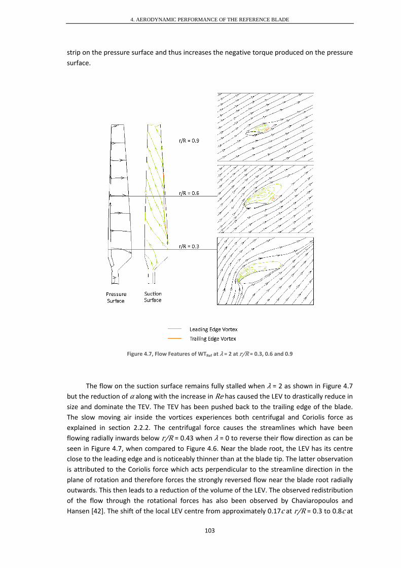
4. AERODYNAMIC PERFORMANCE OF THE REFERENCE BLADE
strip on the pressure surface and thus increases the negative torque produced on the pressure surface.
Figure 4.7, Flow Features of WTRef at λ = 2 at r/R = 0.3, 0.6 and 0.9
The flow on the suction surface remains fully stalled when λ = 2 as shown in Figure 4.7 but the reduction of α along with the increase in Re has caused the LEV to drastically reduce in size and dominate the TEV. The TEV has been pushed back to the trailing edge of the blade. The slow moving air inside the vortices experiences both centrifugal and Coriolis force as explained in section 2.2.2. The centrifugal force causes the streamlines which have been flowing radially inwards below r/R = 0.43 when λ = 0 to reverse their flow direction as can be seen in Figure 4.7, when compared to Figure 4.6. Near the blade root, the LEV has its centre close to the leading edge and is noticeably thinner than at the blade tip. The latter observation is attributed to the Coriolis force which acts perpendicular to the streamline direction in the plane of rotation and therefore forces the strongly reversed flow near the blade root radially outwards. This then leads to a reduction of the volume of the LEV. The observed redistribution of the flow through the rotational forces has also been observed by Chaviaropoulos and Hansen [42]. The shift of the local LEV centre from approximately 0.17c at r/R = 0.3 to 0.8c at
103

4. AERODYNAMIC PERFORMANCE OF THE REFERENCE BLADE
r/R = 0.6 and to the trailing edge at r/R = 0.9 is caused by the reduction of α from the root to the tip and the Coriolis force. The significant size reduction of the vortices increases the torque per unit area on the suction surface and hence the total torque produced by the suction surface.
λ = 4.0
As the rotational speed of the blade further increases, the increase in Re, decrease in α and the rotational effects act together, to shift the LEV further towards the trailing edge and drastically reduce its thickness. The TEV has now completely disappeared. The interaction between the centrifugal and Coriolis force cause the LEV at r/R = 0.3 to be thinner than at r/R = 0.6 when λ = 4 as it is shown in Figure 4.8. Above r/R = 0.9 the favourable flow conditions allow the flow to stay fully attached. The torque performance of the suction surface is further improved due to the reduction of the size of the LEV. However as the separation bubble is very small, the suction surface approaches its optimum torque production at λ = 4 as seen in Figure 4.5.
Figure 4.8, Flow Features of WTRef at λ = 4 at r/R = 0.3, 0.6 and 0.9
104

4. AERODYNAMIC PERFORMANCE OF THE REFERENCE BLADE
At λ = 4 the stagnation point along the entire blade radius has now moved very close to the leading edge of the pressure surface as shown in Figure 4.8. This further reduces the production of useful torque on the pressure surface as the wind experiences a greater adverse pressure gradient.
λ = 0 - 6
An overview of which regions of the suction surface are covered by an LEV or TEV for λ ranging from 0 to 6 is given in Figure 4.9.
Figure 4.9, Area of Suction Surface Covered by LEV and TEV and Stagnation Line on Pressure Surface for λ = 0 - 6 of WTRef
While the TEV rapidly decreases in size as the stationary blade starts to rotate until it diminishes at λ ≈ 2.5, the blade surface covered by the LEV increases when λ < 2 as the LEV extends from the leading edge of the blade to the edge of the TEV. The LEV begins to shift
105

4. AERODYNAMIC PERFORMANCE OF THE REFERENCE BLADE
towards the trailing edge after covering almost the entire suction surface at λ = 2. At λ = 3 the flow begins to fully attach at the blade tip and partially attach down to r/R = 0.7 due to a high Re and low enough α. As λ increases, the region of attachment also increases. When λ = 5, an additional region near the blade root where the flow is fully attached emerges which could be the result of the stall delaying effect of the interaction between the centrifugal and Coriolis force. Hu et al. [41] described a similar effect of the chordwise component of the Coriolis force which acts as a favourable pressure gradient, delaying stall.
Figure 4.9 suggests that when the turbine operates at its optimum cP at λ = 5.5, the flow is fully attached to the aerodynamic section of the blade, only the circular section at the blade root and the transition section below r/R = 0.25 show separated flow. The stagnation point on the pressure surface continuously shifts towards the leading edge as λ increases. When λ > 3 the stagnation line coincides with the leading edge for most of the blade span.
4.3 Reynolds Number Effect
Both, the wind speed at which a turbine operates and its radius affect the Re range experienced by its blades. First a detailed analysis of the effect of scaling the turbine down from a 5.029m radius to a 0.334m radius while maintaining a wind speed of 6m/s is presented. Following is an analysis of the effect of varying the wind speed from 3m/s to 20m/s at both turbine scales. All turbine performance data is presented for λ from λ = 0 up to λ corresponding to the turbine’s highest cP performance.
4.3.1 Turbine Scale
Following is an analysis that investigates the source of the cP and cT differences when scaling the R = 5.029m turbine down to R = 0.334m while maintaining a wind speed of 6m/s for both turbines. Scaling the turbine down reduces its maximum cP by 27% from 0.26 to 0.19 while shifting λ at which the highest efficiency is obtained from 5.5 to 5.4 as shown in Figure 4.10. The corresponding Re at the blade tip reduces from approximately 815,000 for the large scale machine to approximately 53,000 for the small HAWT. The maximum cT obtained reduces by 29% from 0.054 to 0.039. The corresponding λ however is slightly increased from 4.3 to 4.4. For 0 < λ < 2 the cT performance of both turbines is nearly identical, however the following increase in cT with λ occurs at a higher rate for the large turbine than for the small turbine. The remainder of this section investigates the reason for the differences in the turbines cT performances.
106
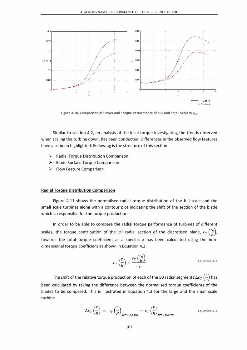
4. AERODYNAMIC PERFORMANCE OF THE REFERENCE BLADE
Figure 4.10, Comparison of Power and Torque Performance of Full and Small Scale WTRef
Similar to section 4.2, an analysis of the local torque investigating the trends observed when scaling the turbine down, has been conducted. Differences in the observed flow features have also been highlighted. Following is the structure of this section:
Radial Torque Distribution Comparison Blade Surface Torque Comparison Flow Feature Comparison
Radial Torque Distribution Comparison
Figure 4.11 shows the normalised radial torque distribution of the full scale and the small scale turbines along with a contour plot indicating the shift of the section of the blade which is responsible for the torque production.
In order to be able to compare the radial torque performance of turbines of different
scales, the torque contribution of the nth radial section of the discretised blade, 𝑐𝑐𝑇𝑇 �𝑟𝑟𝑛𝑛𝑅𝑅�,
towards the total torque coefficient at a specific λ has been calculated using the non-dimensional torque coefficient as shown in Equation 4.2.
𝑐𝑐𝑇𝑇 �
𝑟𝑟𝑅𝑅� =
𝑐𝑐𝑇𝑇 �𝑟𝑟𝑛𝑛𝑅𝑅�
𝑐𝑐𝑇𝑇 Equation 4.2
The shift of the relative torque production of each of the 50 radial segments Δ𝑐𝑐𝑇𝑇 �𝑟𝑟𝑅𝑅� has
been calculated by taking the difference between the normalised torque coefficients of the blades to be compared. This is illustrated in Equation 4.3 for the large and the small scale turbine.
Δ𝑐𝑐𝑇𝑇 �𝑟𝑟𝑅𝑅� = 𝑐𝑐𝑇𝑇 �
𝑟𝑟𝑅𝑅�
𝑅𝑅=0.334𝑚𝑚− 𝑐𝑐𝑇𝑇 �
𝑟𝑟𝑅𝑅�𝑅𝑅=5.029𝑚𝑚
Equation 4.3
107

4. AERODYNAMIC PERFORMANCE OF THE REFERENCE BLADE
Figure 4.11, Effect of Scaling on Normalised Torque Distribution of Small and Large WTRef with Superimposed Geometric α at vw = 6m/s
The spanwise torque distribution of the scaled down turbine is similar to that of the full scale turbine across the full range of λRef. However at λRef ≈ 2 the blade tip of the small turbine which operates in the region of Re ≈ 22,000 is not able to generate as much torque as the tip of the large turbine which operates at Re ≈ 350,000 at the same λRef. The reduction of torque generated at the tip at λRef ≈ 2 is a consequence of the Re effects which are observed for α < 26°. This is in reasonable agreement with Alam et al. [43] who experimentally observed that Re effects become significant when α < 20° for the NACA 0012 aerofoil. The small turbine consequently relies on the torque generated by the root for higher λRef. The comparatively low torque magnitude generated by the root however causes λ at which the small blade experiences a rapid increase in cT as shown in Figure 4.14, to be delayed from λRef ≈ 2 for the large blade to λRef ≈ 2.5 for the small blade. The following increase of cT with λRef, which has been shown to be related to the section of the blade operating at α < 22° for the large turbine in chapter 4.2, is reduced for the small scale blade due to the adverse Re effects. This is caused by lower radial cT increase for the small turbine which also occurs at a higher α of α < 26°.
108

4. AERODYNAMIC PERFORMANCE OF THE REFERENCE BLADE
Blade Surface Torque Comparison
Figure 4.12, Torque Contribution of Suction and Pressure Surface along with Torque per Unit Area Contour for the Small and Full Scale WTRef Operating at vw = 6m/s
109

4. AERODYNAMIC PERFORMANCE OF THE REFERENCE BLADE
A detailed study of the torque distribution along the suction and pressure surface of the small scale turbine is presented in Figure 4.12. The colour coding and the use of hashed areas are identical to that of the full scale HAWT in Figure 4.5. The small scale turbine shows a very similar torque distribution on both blade surfaces to that of the large turbine which is presented in Figure 4.5, for 0 < λRef < 1. This is reflected in the almost identical cT of both blade surfaces in that range. When λRef ≈ 2 however the cT of the pressure surface of the small scale turbine begins to drop below that of the full scale machine. This is caused by an increase of the area of the pressure surface which is covered by a negative pressure. The area is extended towards the trailing edge and hence produces more negative torque. This trend is observed for λRef ≥ 2. The suction surface also shows a reduction in cT when λRef > 2. A slight shift of the torque per unit area towards the root of the suction surface is observed which confirms the interpretation of the radial torque distribution in Figure 4.11. The flow features responsible for this shift have been examined at λRef = 4 where the suction surface experiences a 16% loss in cT while the pressure surface experiences a loss of 38% as a result of scaling the turbine down.
Flow Feature Comparison
Comparing the flow structures of both turbine blades at λRef = 4 in Figure 4.13 indicated that the small turbine experiences significantly more stalled flow along the entire suction surface than the large blade. The large turbine experiences flow detachment at approximately 0.5c from its root to r/R ≈ 0.9 where Re = 620,000. The small blade however only experiences a maximum Re of 42,000 for the same range of geometric α. The significantly lower momentum of the flow causes the point of flow separation to move towards the leading edge as the boundary layer of the smaller turbine cannot withstand the strong adverse pressure which flow around the large scale turbine can. This is reflected by the fully stalled flow on the suction surface of the small blade from its root to r/R ≈ 0.6 where Re = 40,000. The flow remains partially stalled from r/R ≈ 0.6 to the blade tip. The size of the separation bubble formed around the small blade is significantly larger than that around the full scale blade. The small turbine consequently relies on the torque generated at the blade root for longer.
Compared to the full scale turbine, a much larger area of the small scale HATW’s suction surface is covered by a LEV which also has a larger relative diameter than the full scale turbine. The comparatively early flow separation which is caused by the decreased flow momentum acts to reduce the suction surface’s cT. Both pressure surfaces exhibit the same streamline pattern which is also suggested by the identical torque per unit area plots of both turbine scales shown in Figure 4.5 and Figure 4.12.
110

4. AERODYNAMIC PERFORMANCE OF THE REFERENCE BLADE
Figure 4.13, Flow Field of Small Scale and Full Scale WTRef at λ = 4 at r/R = 0.3, 0.6 and 0.9
4.3.2 Varying Wind Speed at Different Turbine Scales
This section investigates the aerodynamic response when subjecting the small and large scale turbines to a wind speed of 3, 6 and 20m/s. Figure 4.14 shows the cP and cT performance of the full scale NREL Phase VI turbine with a radius of 5.029m and the small scale machine with a radius of 0.334m.
The full scale NREL Phase VI turbine shows comparatively little Re effects over the wind speed range tested, while the small turbine shows significant cP and cT variations with wind speed changes due to Re effects. Increasing vw from 6 to 20m/s increases the maximum cP performance of the large turbine by 5%, however it accounts for a 24% improvement of the small turbine. Decreasing vw from 6 to 3m/s reduces the maximum cP of the large turbine by only 4% but it reduces the small turbine’s performance by 40%. When the turbine is stationary however it produces cT = 0.0075 regardless of the wind speed or turbine scale. Up until λRef ≈ 2, the cT of both turbine scales operating at all vw is very similar, indicating that the flow is Re independent when 0 ≤ λ < 2 due to the heavy stall of the flow. The cause for the nonlinear interaction of the Re effects at higher λ due to scaling and changing winds has been investigated.
111

4. AERODYNAMIC PERFORMANCE OF THE REFERENCE BLADE
Figure 4.14, Power and Torque Performance of Small and Large Scale NREL Phase VI Blade
Figure 4.15 shows the cT of the small and large scale turbines operating at vw = 6m/s from λRef = 0 up until λ at which the turbines achieve their highest cP. In order to gain a better understanding of how varying wind speed affects both turbine scales, the difference in the torque coefficient Δ𝑐𝑐𝑇𝑇(𝑟𝑟), when the turbines operate at 3 and 20m/s has been evaluated with respect to the 6m/s performance as shown in Equation 4.4.
Δ𝑐𝑐𝑇𝑇(𝑟𝑟) = 𝑐𝑐𝑇𝑇(𝑟𝑟)𝑣𝑣 − 𝑐𝑐𝑇𝑇(𝑟𝑟)𝑣𝑣=6𝑚𝑚/𝑟𝑟 Equation 4.4
The change in cT shows a clear correlation to the local α for the small and large scale turbines. The range of α, and hence the range of λ, during which a large cT variation is, observed is related to the local Re. When decreasing vw from 6 to 3m/s, the full scale blade first experiences a performance reduction of approximately 50% at the blade tip when α first falls in the range of 21° < α < 27°. This occurs at λRef ≈ 2.3 and is accompanied by a Re reduction from 390,000 to 190,000 when reducing vw from 6 to 3m/s. As λ increases further, the section of the blade experiencing a performance reduction shifts radially inwards in accordance with the range of α prone to a performance reduction. The Re effects become weaker towards the blade root until they almost disappear when r/R < 0.5 at λRef ≈ 3.5. This is in agreement with the streamline plots of both turbines presented in Figure 4.13, which shows that the shape of the LEV across different turbine scales becomes more similar towards the blade root for λ = 4.
When increasing vw from 6 to 20m/s, an improvement of up to 100% in the turbine’s cT performance is observed. The trend of the blade sections showing Re effects at different λ is similar to the one previously discussed. However the significantly higher Re’s encountered cause the range of α prone to Re effects to slightly increase to 22° < α < 28°. This is due to the increased momentum of the flow which allows it to stay attached to the blade at a higher α when vw increases. The relatively uniform strip of the cT variation along the blade in Figure
112

4. AERODYNAMIC PERFORMANCE OF THE REFERENCE BLADE
4.15 causes a change in vw to merely offset λ at which the large scale turbine experiences a rapid increase of its cT with λ, but not modify its cT - λ gradient as is shown in Figure 4.14.
Figure 4.15, Effect of Wind Speed at Different Turbine Scales of WTRef, Reference Wind Speed is 6m/s
113

4. AERODYNAMIC PERFORMANCE OF THE REFERENCE BLADE
The scaled down blade shows a different response to changing vw. When reducing vw from 6 to 3m/s, the turbine starts to experience significant Re effects when α < 20° which first occurs at the blade tip at λRef ≈ 2.5. There is no lower limit of α at which Re effects occur due to the ultra-low Re range at which the small scale turbine operates. This causes the overall cT of the small turbine to continuously decrease when lowering vw as seen in Figure 4.14. When increasing vw from 6 to 20m/s, the angle of attack at which Re effects are observed increases to α < 23°. This is similar to the findings of the large scale turbine. However the much larger and not uniformly distributed operating range affected by Re effects, causes the cT vs. λ curve of the small turbine to drastically lower the gradient at which the overall cT rises up to its maximum value when λRef > 2.4. This is also seen in Figure 4.14.
4.4 Summary
This chapter introduced the performance of the full scale NREL Phase VI turbine which has been used as a reference for the evaluation of different blade designs in chapter 5. A detailed analysis of the turbine operating at the reference wind speed of 6m/s revealed important relations between its geometry and the flow structure around the blade, the spanwise torque distribution as well as the torque distribution on the blade surfaces. The analysis was then extended to investigate Reynolds number effects by examining a 5.029m scale and a 0.334m scale turbine operating at wind speeds of 3, 6 and 20m/s.
Reference Case
When the turbine is stationary it produces a torque coefficient of 0.0075 of which the pressure surface contributes 63% while the suction surface only produces 27%. The flow approaching the pressure surface parts at the chord-wise location where the local blade curvature is parallel to the rotational plane. It forms a comparatively large LEV and TEV behind the suction surface. A high Reynolds number, which occurs at large blade chords, was associated with an increase of the relative size of the vortices. The LEV was found to dominate the TEV when the blade twist is high. The suction surface consequently experiences a negative pressure field of relatively low magnitude due to the vortices. The pressure field only translates to positive torque near the leading edge of the blade and at the blade root. The positive pressure on pressure surface, in contrast, produces a negative torque over a comparatively small area at the leading edge and a positive torque at the trailing edge. The resulting torque distribution along the blade radius is relatively uniform.
When the turbine starts to rotate, the majority of the torque is produced between 25 and 30% radius until the tips speed ratio is approximately 2. This is a consequence of the nearly uniformly distributed Reynolds number along the blade span at this tip speed ratio which makes the lift and drag production predominantly a function of the angle of attack. The
114

4. AERODYNAMIC PERFORMANCE OF THE REFERENCE BLADE
comparatively low angle of attack at the root therefore causes a high torque production in that region. The good performance of the blade root is further enhanced by rotational effects. The interaction between the separated flow and the centrifugal and Coriolis force causes the LEV to become thinner at the blade root. The decrease in the size of the LEV and TEV causes the torque to increase on the suction surface. The pressure surface in contrary experiences a reduction of its torque which can be linked to the formation of a negative pressure region, at about half chord. The blade produces a torque coefficient of 0.011 at a tip speed ratio of 2 of which the suction surface contributes 131%.
A further increase in rotational speed leads to a rapid increase in the blade’s torque coefficient which is initiated by the decrease of the angle of attack to below 22° at the blade tip. The large increase in torque continues until the entire upper half of the blade operates at an angle of attack of less than 22°. When the tip speed ratio reaches 4.3, the blade achieves its maximum torque coefficient of 0.054, although the flow around the suction surface is still partially stalled. The torque of the suction surface continues to gently increase until the flow is full attached at a tip speed ratio of approximately 5.5. The performance of the blade is therefore limited by the generation of negative torque on the pressure surface. The pressure surface generates increasingly more negative torque due to larger parts of the blade surface experiencing a negative pressure.
Reynolds Number Effect
Scaling the turbine down while maintaining a constant wind speed does not affect the turbine’s performance when it operates at a tip speed ratio of less than 2 due to the heavy stall of the flow. Above that tip speed ratio however the torque coefficient generated by both blade surfaces reduces. The pressure surface of the small scale turbine experiences a larger area of negative pressure than that of the full scale turbine, while the flow around the suction surface of the smaller turbine is subjected to a greater stall due to the lower momentum of the flow. This results in the reduction of the maximum torque coefficient of 29%.
Both turbine scales were found to react differently to variations in operating wind speed. The full scale turbine only shows a wind speed dependent variation in its radial torque when the angle of attack is in the range of approximately 22° to 28° due to the relatively high Reynolds numbers it is subjected to. This results in the blade section affected by Reynolds number effects to move radially inwards from the blade tip as the blade speed increases. The torque coefficient of the full scale blade therefore shows comparatively little variation with wind speed. The small scale turbine however is greatly affected by wind speed variations as all angles of attack below approximately 23° induce Reynolds number effects. Reynolds number effects first occur at the blade tip and then propagate radially inwards with increasing tip speed ratio until the entire blade experiences Reynolds number effects. The small blade consequently shows a much lower torque coefficient than its full scale counterpart. This trend becomes more pronounced for low wind speeds.
115

5. AERODYNAMIC ANALYSIS OF BLADE PARAMETERS
5.1 Introduction
This chapter investigates the effect of important blade design parameters by varying the design of the reference turbine whose performance has been established in chapter 4. This forms the background for the analysis of the respective turbine starting sequences in chapter 6. The role of pitch, blade thickness and their combined effect has been studied as outlined in Figure 5.1. The first two studies examine the role of increasing the blade pitch from 0° to 10° and decreasing the blade thickness from 21% to 15% while a third study investigates the performance of a rotor with blades of 15% thickness which are pitched by 10°.
Figure 5.1, Investigated Rotor Pitch and Blade Thickness Configurations of WTRef, WTP, WTT and WTP-T

5. AERODYNAMIC ANALYSIS OF BLADE PARAMETERS
The different blade designs have been analysed in terms of their torque and power performance as well as their aerodynamics. While the power analysis gives information about the blade’s performance when it operates at its design tip speed ratio, the torque properties below that tip speed ratio give information on the blade’s starting characteristics which have been analysed in chapter 6. The investigations of each blade have been conducted for rotational speeds from 0rpm up to the corresponding blade’s design tip speed ratio using the performance evaluation criteria established in chapter 4. The performance of the geometrically modified blades has been compared in detail to that of the reference blade at radius of 5.029m and a wind speed of 6m/s. Following this is a comparative analysis of the Reynolds number effects on the new blade designs. The analysis was extended to cover turbines with a radius of 5.029m and 0.334m operating at wind speeds of 3, 6 and 20m/s. Again, particular emphasis has been given to the torque performance as this dictates the turbine’s starting behaviour analysed in chapter 6. Modifying the blade thickness or pitch leads to changes in the blade’s power and torque performance due to 2 distinct mechanisms:
• Flow Features: At a given tip speed ratio the wind approaching the turbine will encounter a blade with a thinner aerodynamic profile or experience a different angle of attack and thus produce different flow features which results in changes in the blade surface pressure distribution and turbine torque.
• Blade Curvature: Even when assuming the same pressure distribution for different blade designs, the difference of the curvature of the blade surfaces with respect to the rotational plane acts to produce a different torque distribution and consequently produces a different net torque.
To place the research conducted in this thesis into context in the wider body of knowledge this section is finally concluded with an analysis of the applicability of lower order BEM methods to accurately model the effect of different turbine blade designs on their cP. A comparison between CFD methods and BEM methods for WTRef is shown in section 3.3.4. The analysis was conducted with respect to the previously obtained CFD results from this chapter.
5.2 Role of Blade Pitch
This section investigates the effect of pitching the reference turbine, which has a blade thickness of 21%, by 10°. The relatively large pitch angle of 10° has been chosen, based on the literature published on the effect of blade pitch in section 2.4.3, to be able to clearly identify the effect of pitching on the turbine performance. Following is a detailed investigation of the effect of blade pitch on the torque distribution and the flow features. Pitching the blade affects the local α which in turn modifies the flow structures and the surface curvature. Both aspects have been discussed in this section.
117

5. AERODYNAMIC ANALYSIS OF BLADE PARAMETERS
The analysis shows observed trends in the torque of the pitched blade for a range of λP and compares it to the reference blade, λRef, while the flow feature analysis provides background information on the differences in flow features and hence turbine performances. Furthermore, an overview of the effect of pitching the blade has been given for a larger range of wind speeds and different turbine scales.
5.2.1 Torque Performance at Reference Condition
This analysis is conducted at a 5.029m turbine scale. Increasing the blade’s pitch by 10° significantly changes the turbine’s cP and cT performance as can be seen in Figure 5.2 where the performance of the pitched and un-pitched turbines have been compared at a wind speed of 6m/s. The cT generated by the pitched turbine is increased by 79% from 0.0075 to 0.0134 when it is stationary. Similarly to the reference turbine, the pitched turbine also experiences a slight initial reduction in cT as λ increases. However the pitched rotor’s cT begins to rapidly increase when λP ≈ 1.4, for the un-pitched blade this only occurs at λRef ≈ 2.3. The rapid increase of cT occurs at a similar gradient for both turbines, but the turbine with pitched blades reaches an optimum cT of 0.042 which is 22% lower than that of the un-pitched blade at a much lower λ than the un-pitched blade. This results in the pitched blade attaining a maximum cP of only 0.127 at λP = 3.2 while the un-pitched blade attains a cP of 0.262 at λRef = 5.5. The reason for the increase in cT and its shift towards lower λ when pitching the blade is discussed in this section. A detailed analysis comparing the local torque features of the reference turbine to those of the pitched turbine has been conducted:
Radial Torque Comparison Blade Surface Torque Comparisons
Figure 5.2, Power and Torque Performance of WTP and WTRef at 6m/s at R = 5.029m
118

5. AERODYNAMIC ANALYSIS OF BLADE PARAMETERS
Radial Torque Comparison
Pitching the blade by 10° reduces the geometric local α by the same amount along the blade for a given λ. This is shown in Figure 5.3 which illustrates the shift in the normalised radial torque distribution superimposed with the local α for the pitched and un-pitched blades. The difference of the normalised torque produced by each blade section is also illustrated to show the shift of the relative torque distribution for all λ.
Figure 5.3. Normalised Torque Distribution of Pitched (WTP) and Un-Pitched (WTRef) Blade with Superimposed Geometric α
Three characteristic differences between the torque distributions of both blade configurations have been observed as a result of pitching the blade:
• When the blade is stationary a slight shift of the section of the blade responsible for the majority of the torque production towards the blade tip has been observed when comparing WTP with WTRef.
119

5. AERODYNAMIC ANALYSIS OF BLADE PARAMETERS
• When λ rises to 0 < λP < 2.3, the pitched blade experiences a much less pronounced shift of the torque production region towards the root of the blade. The lower α allows the blade tip to perform significantly better and not produce a negative torque as it has been observed at the tip of the reference blade.
• Reducing α by 10° by pitching the blade causes α at the blade tip to drop below 22° when λP ≈ 1.5 instead of only at λRef ≈ 2.5. This is the cause for the earlier rapid increase of cT with λP in Figure 5.2, as α < 22° has been shown to be associated with a high cT production in section 4.2.1.
Blade Surface Torque Comparisons
Before analysing the torque distribution of the pitched blade for specific λP’s, the effect of modifying the turbine geometry on the translation from static pressure to torque is briefly discussed analogously to section 4.2.1. Figure 5.4 shows the blade curvature of the pitched pressure and suction surfaces along with the zero-blade-curvature line of WTP and WTRef.
Figure 5.4, Blade Curvature of Suction and Pressure Surface of Pitched Blade (WTP) Along with Zero-Blade-Curvature-Line of WTP and WTRef
When comparing the blade curvature of both blades, a shift of the zero-blade-curvature line on both blade surfaces was observed. The zero-blade-curvature line on the pressure surface of the pitched blade is shifted towards the leading edge which results in the pressure
120

5. AERODYNAMIC ANALYSIS OF BLADE PARAMETERS
surface of the pitched blade producing a higher torque than that of the reference blade when both surfaces are subjected to the same uniform positive pressure. This is because the area near the leading edge producing negative torque has decreased while the area near the trailing edge which produces positive torque has increased. The zero-blade-curvature line on the suction surface of WTP in contrast is shifted right to the trailing edge. This acts to produce positive torque for a negative pressure on the entire aerodynamic section of the suction surface. For a given uniformly distributed negative pressure, the suction surface of the pitched blade therefore also outperforms the reference blade. It can be concluded that the pitched blade is better at translating a given pressure distribution into useful torque from a geometrical aspect.
A detailed analysis of the distribution of the torque per unit area contour on both blade surfaces of the pitched blade, together with the total torque contribution of each surface is presented in Figure 5.5. The blade surface torque has been compared to the torque distribution of the reference turbine shown in Figure 4.5. When pitching the blade, the suction surface generates a higher cT for all λP. This is due to the exclusive formation of positive torque on the suction surface of WTP which results from a negative pressure along the suction surface that is observed throughout the entire range of λP. Up until WTP reaches its highest cP, the suction surface of the pitched blade generates more cT than that of the un-pitched blade. The pitched pressure surface in contrast only generates a higher cT to WTRef when λP < 1.15, at higher λP the pitched blade produces a similar cT to the un-pitched blade. Consequently, the corresponding distribution of the torque per unit area of the pitched blade differs significantly from that of the reference blade. The pitched blade generally shows lower torque intensities when comparing corresponding λ’s, additionally a change in flow features and a shift of the blade curvature and the zero-blade-curvature line are responsible for different cT’s. A detailed discussion on the absolute torque and torque distribution for λP between 0 and 3 follows.
When the blade is stationary, the cT performance of the pitched pressure surface is increased by 50% which is caused by both, the shift of the zero-blade-curvature line as shown in Figure 5.4 as well as a change in the pressure distribution. Figure 5.5 shows that the positive pressure at the leading edge of the pressure surface of WTP is very low. This pressure reduction of WTP is caused by a comparatively low blade curvature of the pitched pressure surface in that region and acts to reduce the negative torque generation of the pressure surface of WTP compared to WTRef. The suction surface of the pitched blade particularly benefits from the shift of the zero-blade-curvature line which eliminates the area between the zero-blade-curvature line and the TE. This area had been responsible for the generation of negative torque of the suction surface of WTRef. The torque generated by the pitched suction surface is therefore 2.2 times that of the reference blade. The effect of the blade curvature on the torque distribution of both blade surfaces of WTP dominates that of the flow features. This is in agreement with the observed dependence of the reference turbine’s cT on the blade curvature rather than specific flow features as it been presented and explained in section 4.2.1 and 4.2.2. The net torque of both blades is heavily influenced by relative sizes of the areas enclosed between the LE and the zero-blade-curvature line as well as the zero-blade-curvature line and the TE. However in contrast to the reference blade, the majority of the useful torque of WTP is produced by the upper blade half near the leading edge. This is also reflected in the shift of the radial torque towards the blade tip in Figure 5.3.
121

5. AERODYNAMIC ANALYSIS OF BLADE PARAMETERS
Figure 5.5, Torque per Unit Area Contour of WTP along with Torque Contribution of Suction and Pressure Surface of WTP and WTRef
When λP = 1 the negative cT of the pitched pressure surface is comparable to that of the un-pitched blade. The positive pressure on the pitched pressure surface has risen to produce a negative torque on the leading edge. However the negative torque per unit area of the pitched blade is considerably lower than that of the reference blade. The pitched pressure surface was also observed to have a high enough pressure drop in the chordwise direction to produce a negative pressure region at the blade tip, downstream the zero-blade-curvature line. This torque reducing phenomenon is only observed for higher λ when the blade is not pitched. The suction surface however compensates for the relatively poor performance of the pressure surface by generating 1.9 times the torque of the un-pitched suction surface. The majority of the torque is generated between the leading edge and 0.5c as well as at the blade root below r/R ≈ 0.3. In contrast to the reference blade, the suction surface of the pitched blade does not generate negative torque.
122

5. AERODYNAMIC ANALYSIS OF BLADE PARAMETERS
As the rotational speed of the blade increases, the negative torque per unit area at the LE of the pitched pressure surface becomes more negative. Meanwhile the area of the pressure surface which is subjected to negative pressure also rapidly increases by extending in the chordwise direction and radially inwards. Both factors cause the cT of the pressure surface to drop below 0 at λP = 1.5. When λP = 2 the strip of negative pressure extends along the entire length of the pitched blade, this is only observed for λRef ≥ 4 when the blade has 0° pitch. The onset of the negative pressure formation therefore not only occurs at a lower λ when the blade is pitched, but also shows a higher sensitivity to increasing λ. When λP = 2, the torque per unit area of the pitched suction surface has yet again considerably increased which allows the pitched suction surface to generate 2.1 times the torque of the reference blade’s suction surface. The entire WTP suction surface experiences an increase in torque per unit area with the highest increase of the torque per unit area at the leading edge when r/R > 0.7. The upper half of the suction surface’s trailing edge which has been observed to generate negative torque in the un-pitched configuration now also contributes towards a high cT of the pitched rotor by generating positive torque.
When λP = 3 the root of the pitched pressure surface completely loses its positive torque generating ability, this trend has also been observed for the reference blade but to a lesser degree. However, the larger spread of negative torque near the leading edge of the reference blade at the same λ causes both pressure surfaces to produce a comparable cT. The torque production of the pitched suction surface is also shifted towards the leading edge as the trailing edge loses its torque producing ability. The blade root region suffers a considerable loss in torque, resulting in a much more uniformly distributed radial torque for the pitched blade than for the reference rotor. This has also been captured in the radial torque distribution of both WTs in Figure 5.3. Following is an analysis of the flow features explaining the differences of the torque formation observed in this section.
5.2.2 Flow Field at Reference Conditions
Based on the previously observed differences in the radial torque distribution, the flow features have been analysed at 3 different λP’s:
λP = 0.0 gives information on the improved cT performance of the stationary pitched blade.
λP = 1.5 shows how the flow features develop for increasing rotational speed. λP = 3.0 illustrates significant flow features close the pitched turbine’s optimum cP
performance.
As it has been shown in chapter 4 for the reference blade, the local α along the blade dominates the turbine’s aerodynamics, Re effects are of secondary nature. However when pitching a blade, for a given λ and radial location r/R, the local Re is not altered but the local α decreases by the amount the blade is pitched by. The comparison between the performance of the pitched blade and the reference blade has therefore been carried out over a range of λ using the following 2 criteria in order to better differentiate between effects due to Re and α:
123

5. AERODYNAMIC ANALYSIS OF BLADE PARAMETERS
• λRe denotes the tips speed ratio of the reference turbine, λRef , when preserving the geometrical Re for the comparison of the flow features of the pitched and un-pitched rotors at the same r/R location. α is not preserved.
• λα indicates λRef of the reference turbine in order to compare both blades operating at the same geometrical α for a given r/R location. Re is not preserved. The mathematical correlation between λRef and the pitched turbine λP is given in Equation 5.1 for a rotor pitch angle difference of 10°.
𝜆𝜆𝑅𝑅𝑛𝑛𝑅𝑅 = 1
tan�tan−1 � 1 𝑟𝑟 𝑅𝑅� 𝜆𝜆𝑃𝑃
� − 10°�
𝑟𝑟𝑅𝑅
� Equation 5.1
In order to compare the flow field of WTP with that of WTRef using both comparison criteria, Figure 5.6 visualises the required rotational speed of WTRef when using λP = 0, 1.5 and 3 as a reference rotational speed. While λRe of the reference turbine does not deviate from λP, the required λα has been calculated using Equation 5.1 to compare both turbines as they operate at the same geometrical α at the same r/R location. It can be seen that the difference between λP and λα increases for increasing λP. This trend is more pronounced at the blade tip than at the blade root.
Figure 5.6, Contour of Geometric α for WTP and WTRef Labelled with Investigated Configurations of WTP (r/R = 0.3, 0.6 and 0.9, λP = 0.0, 1.5 and 3.0) and Corresponding λRe and λα Positions for WTRef
Using λRe and λα, the performance of the reference turbine can now be used as an indicator for the effect of pitching the blade. While λRe is expected to considerably underestimate the performance of the pitched blade due to an unfavourable α of the reference blade, λα is expected to only slightly overestimate the pitched turbine’s performance. The overestimation is a consequence of the associated increase in the local Re, which is only of secondary importance for the flow structure. The analysis of the flow around
124

5. AERODYNAMIC ANALYSIS OF BLADE PARAMETERS
the pitched blade for λP = 0, 1.5 and 3 and the corresponding λRe and λα of the reference blade is presented in Figure 5.7, Figure 5.8 and Figure 5.9 respectively. The flow structures presented for λRe and λα have been rounded to the nearest 0.5 λ. This analysis provides both, information on the flow features corresponding to the lower performance bound for the pitched turbine as well as for the upper performance bound. Variations in the LEV and TEV and their respective sizes and the location of the vortex centres have been investigated.
λP = 0.0
Figure 5.7, Comparison of Flow Features around Pitched (WTP) and Un-Pitched (WTRef) Blade at λP = λRe = 0.0, λRe = 0.0, 0.0 and 0.5 and at r/R = 0.3, 0.6 and 0.9 respectively
125

5. AERODYNAMIC ANALYSIS OF BLADE PARAMETERS
When the blade is stationary the flow approaching the pressure surface of the pitched blade parts near the zero-blade-curvature line, similarly to the flow approaching the reference blade. The stagnation line is therefore shifted closer to the leading edge as it can be seen in Figure 5.7 for λ = 0. The flow pattern along the suction surface does not vary significantly when changing the blade pitch compared to the reference blade. However the reduction of α and a mild circulation around the blade in the clockwise direction act together to amplify the domination of the LEV to the TEV when comparing λP of the pitched blade to λRe of the un-pitched blade.
Although the pitched blade experiences a local angle of attack that is reduced by 10° compared to the reference blade, the flow behind the suction surface remains fully stalled as the adverse pressure gradient imposed on the flow is still too high for the flow to remain attached. The very high α, which is in the range of 58° at the pitched blade’s root, to 80° at its tip, causes the formation of an LEV and a TEV along the entire blade radius. The vortices at λRe are similar to those observed behind the reference blade at λRef = 0. To preserve α, the flow features at r/R = 0.3, 0.6 and 0.9 have been illustrated using λα ≈ 0.5, 0.5 and 0.0 respectively. This results in an increasing underestimation of the size of the vortex pair towards the blade root which is caused by the more favourable α and the addition of rotational effects when λα > 0. The Coriolis and centrifugal force drastically reduce the size of the vortices at the blade root as discussed in detail in section 4.2.2. Due to the similar flow feature formation between λP and λRe, the greatly improved cT performance when pitching the blade by 10° is predominantly the result of the more favourable pressure to torque translation of the pitched blade, which is described in section 5.2.1, rather than a significant change in the flow features.
λP = 1.5
As the rotational speed increases, the observed flow structures around the pitched and un-pitched blades operating at the same λ begin to deviate, which makes the improved cT performance of the pitched blade a function of both, the different pressure-torque translation and a change in the flow features. Figure 5.8 shows the flow when the reference blade operates at λP = 1.5 and for corresponding λRe and λα. Pitching the blade has shifted the stagnation line on the pressure surface closer to the leading edge than that of the reference blade as it can be seen in the λRe graphs. This shift along with the change of the local blade curvature and the reduction in α, contribute to the earlier onset of the negative pressure formation at the tip of the pressure surface of the pitched blade. The cT of the pitched pressure surface thereby drops to a similar value to that of the reference blade.
126

5. AERODYNAMIC ANALYSIS OF BLADE PARAMETERS
Figure 5.8, Comparison of Flow Features around Pitched (WTP) and Un-Pitched (WTRef) Blade at λP = λRe = 1.5, λRe = 2.5, 2.0 and 2.0 and at r/R = 0.3, 0.6 and 0.9 respectively
127

5. AERODYNAMIC ANALYSIS OF BLADE PARAMETERS
Although the pitched blade’s suction surface outperforms the cT of the reference blade, the streamline patterns on the suction surfaces are similar when they operate at λP = λRe = 1.5. The pitched blade however shows a slightly larger area which is covered by a TEV near the trailing edge. The TEV of the reference blade ranges from r/R ≈ 0.3 to the tip and extends by a maximum of 0.15c. The suction surface of the pitched blade only experiences a TEV in the range of 0.35 < r/R < 0.8 with a maximum width of 0.08c. The shapes of the vortices in the cross sectional plane however show significant differences. For all 3 radial locations analysed, the streamline patterns around the pitched blade are now beginning to become more similar to those produced by λα than those produced when preserving Re, λRe. From root to tip, λα ≈ 2.5, 2.0 and 2.0 for r/R = 0.3, 0.6 and 0.9 respectively. At the blade root the differences in the flow features between λRe and λα are more pronounced than at the blade tip. This is due to the high flow feature dependence on α when λP = 1.5 and the stronger rotational forces at the blade root for λα as it rotates at a higher rotational speed than λRe. At r/R = 0.3 the LEV of the pitched blade has a maximum thickness of approximately 0.29c, at the same radial location the reference blade shows an LEV thickness of 0.51c and 0.17c for λRe and for λα respectively. A shift of the LEV centre towards the leading edge of the pitched blade has also been observed. This shift of the vortex centre becomes more pronounced with decreasing LEV thickness. The pitched blade’s LEV centre is at approximately 0.29c whereas the reference blade’s LEV centre is at ≈ 0.40c and 0.11c for λRe and λα respectively. Towards the blade tip, differences in flow features between λP, λRe and λα become less pronounced and the vortex pattern of λP becomes more similar to that of λα. Compared to λRe pitching the blade reduces the size of the LEV by approximately 22% at r/R = 0.6 and 19% at r/R = 0.9.
λP = 3.0
The streamlines at λP = 3 which is close to the pitched turbine’s optimum λ for the highest cP and cT production, are presented in Figure 5.9. The suction surfaces of the pitched and un-pitched blades experience significantly different flows. The flow around the suction surface of the reference blade is fully stalled from the blade root to r/R ≈ 0.7 and remains partially stalled thereafter. It separates from the leading edge at approximately 0.4c. The flow on the pitched suction surface in contrast is only partially stalled from the blade root to r/R ≈ 0.65, it detaches from the suction surface at approximately 0.35c. The flow is fully attached from r/R ≈ 0.65 to the blade tip. The different flow structure is also reflected in the very different formation of the LEV and TEV when comparing λP, λRe and λα. The cross sectional flow of λP now shows much higher similarity to λα than to λRe for the entire blade span. While when preserving α only a thin LEV is observed at the blade root of the reference blade, when preserving Re the comparatively high angle of attack of 26° < α < 31° at r/R ≤ 0.6 causes the formation of a large LEV and a small TEV for r/R < 0.65. At r/R = 0.9 both λP and λα show no flow separation but at λRe an LEV of ≈ 0.13c thickness is observed. At r/R = 0.6 a very thin LEV of ≈ 0.01c is observed at λα, λP shows a slightly larger LEV of ≈ 0.04c while λRe indicates a massive LEV of approximately 0.58c thickness along with a TEV. Towards the blade root the differences in the vortex sizes become less severe and the flow features of λP are closer to λα than to λRe.
128

5. AERODYNAMIC ANALYSIS OF BLADE PARAMETERS
Figure 5.9, Comparison of Flow Features around Pitched (WTP) and Un-Pitched (WTRef) Blade at λP = λRe = 3.0, λRe = 4.5, 5.0 and 6.0 and at r/R = 0.3, 0.6 and 0.9 respectively
129

5. AERODYNAMIC ANALYSIS OF BLADE PARAMETERS
The shift of the vortex size which becomes more pronounced as the pitched turbine rotates at higher rotational speeds, significantly contributes towards the improved cT performance of the pitched rotor compared to the un-pitched turbine.
5.2.3 Effect of Reynolds Number
The role of pitching on different turbine scales operating at different wind speeds has been investigated. Figure 5.10 gives an overview of the effect of pitching on cP and cT for the 0.334m scale machine and the 5.029m machine operating at 3, 6 and 20m/s. Similarly to how it has been observed for the reference blade in chapter 4.3.2, the cT of the stationary pitched turbine does not vary with wind speed or turbine scale, although it is increased by 79% compared to that of WTRef.
Figure 5.10, Power and Torque Performance of WTP in Comparison with WTRef at Turbine Scales 0.334m and 5.029m Radius Operating at 3, 6 and 20m/s
130

5. AERODYNAMIC ANALYSIS OF BLADE PARAMETERS
When pitching the large scale machine from 0 to 10° the design cP is reduced by 51% at all wind speeds. Pitching the small scale machine shows a slightly wider spread reduction of the maximum attainable cP of 49-55% as the wind speed varies from 3 to 20m/s. Although the maximum attainable cP scales almost linearly with turbine scale at each wind speed, a detailed analysis of cT showed that there is a significant nonlinear interaction between turbine pitch and turbine scale. The cT performance of the WTs have been analysed in detail in Figure 5.11 as it is of great significance for turbine starting investigated in chapter 6.
Figure 5.11, Effect of Blade Pitch Comparing Total Torque Distribution of WTP with WTRef at Turbine Scales 0.334m and 5.029m at vw = 6m/s
Figure 5.11 shows the cT change that is associated with changing the turbine pitch. The analysis has been conducted for both turbine scales in order to analyse the Re dependence on the effect of pitching. The detailed cT curves of WTRef and WTP of both scales operating at a wind speed of 3m/s visualise the concept behind the analysis. Results are presented for wind speeds of 3, 6 and 20m/s. The large scale machine operates at a near Re independent range which can be seen at the relatively consistent cT improvement due to pitching at all vw. The small scale turbine however experiences a great nonlinear interaction between pitching and Re. Although at 0 ≤ λ ≤ 1.4 the pitching benefit of the small scale machine is close to that of
131

5. AERODYNAMIC ANALYSIS OF BLADE PARAMETERS
the full scale rotor, at higher λ the cT benefit increases rapidly with increasing wind speed. The consistent cT benefit at low λ across all wind speeds and turbine scales is a consequence of the highly stalled flow in that region which removes Re effects. At λ > 1.4 the reduced Re of the small scale machine, particularly when it operates at low vw, causes a delay in the flow attachment mechanism as it has been described in section 4.3 for WTRef. This introduces a strong vw dependence of the small scale turbine where a wind speed of 20m/s is associated with a cT improvement of nearly twice of that achieved at 3m/s. Even at 20m/s the improvement of the small scale turbine is below that of the full scale rotor. A detailed investigation of the torque, analysing the difference of the radial cT between the βPitch= 0° and βPitch = 10° configuration for the 0.334 and the 5.029m scale machines at vw = 6m/s, revealed the underlying reasons for the small turbine’s underachievement.
Figure 5.12, Effect of Blade Pitch Comparing Radial Torque Distribution of WTP with WTRef at Turbine Scales 0.334m and 5.029m at vw = 6m/s
In Figure 5.12 the effect of pitching both turbine scales on the radial cT distribution has been visualised. The interaction between the blade pitch and Re effect has been evaluated by subtracting the radial cT of WTRef from that of WTP for each turbine scale. The large and small scale machines exhibit a similar radial torque pattern over 0 ≤ λ ≤ 3.15. But the relative under-achievement of the scaled down, pitched turbine is initiated from λ ≈ 1.5 as the cT of the small pitched turbine thereafter increases at a significantly lower rate than that of the large pitched rotor. The large rotor operates in a Re range of 146,000 to 509,000 while the small rotor experiences a lower Re of 9,700 to 34,000. This leads to adverse Re effects of the small turbine which cause the large rotor to benefit significantly more from pitching when the angle of attack of the pitched rotor is in the range of 10° < α < 20°. The pitched blade first experiences α < 20° at the blade tip when λP ≈ 1.5 which thereby initiates the underachievement of the small turbine. The underachievement of the small rotor is
132

5. AERODYNAMIC ANALYSIS OF BLADE PARAMETERS
terminated at λP = 3.15 because the torque penalty for pitching at the blade tip and root is more severe for the large machine.
5.3 Role of Blade Thickness
The effect of blade thickness has been investigated in this section. The performance of the reference turbine has been compared to that of a rotor with the same specifications but thinner blades. The reference blade is entirely composed of the S809 aerodynamic profile which has a thickness of 21%. The thin blade uses the same profile but with a reduced thickness of 15%. Both blades operate at 0° pitch. Relevant torque and flow structures are discussed in detail over a range of λ to build an understanding for the effect of blade thickness. The section is concluded with an investigation analysing the interaction between the blade thickness effects and Re effects by varying wind speed and blade scale.
5.3.1 Torque Performance at Reference Conditions
The effect of reducing the blade thickness from 21% to 15% on the turbine’s cP and cT is shown in Figure 5.13 for 5.029m radius turbines operating at a wind speed of 6m/s.
Figure 5.13, Power and Torque Performance of WTT and WTRef at 6m/s at Radius 5.029m
Reducing the blade thickness has a very little effect for λ < 2.2, thereafter the cT of the thin blade increases at a lower rate with λ than for the reference blade. The 15% thickness blade reaches a peak cT of 0.0521 which is 4% lower than that of the reference blade.
133
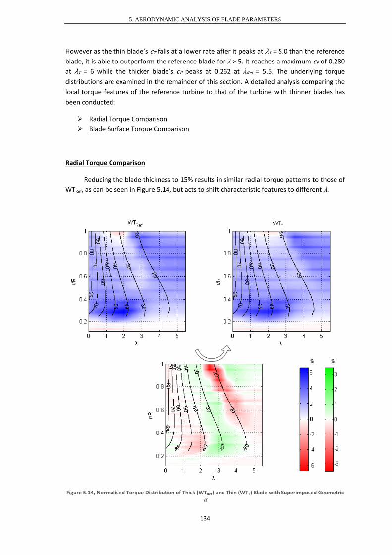
5. AERODYNAMIC ANALYSIS OF BLADE PARAMETERS
However as the thin blade’s cT falls at a lower rate after it peaks at λT = 5.0 than the reference blade, it is able to outperform the reference blade for λ > 5. It reaches a maximum cP of 0.280 at λT = 6 while the thicker blade’s cP peaks at 0.262 at λRef = 5.5. The underlying torque distributions are examined in the remainder of this section. A detailed analysis comparing the local torque features of the reference turbine to that of the turbine with thinner blades has been conducted:
Radial Torque Comparison Blade Surface Torque Comparison
Radial Torque Comparison
Reducing the blade thickness to 15% results in similar radial torque patterns to those of WTRef, as can be seen in Figure 5.14, but acts to shift characteristic features to different λ.
Figure 5.14, Normalised Torque Distribution of Thick (WTRef) and Thin (WTT) Blade with Superimposed Geometric α
134

5. AERODYNAMIC ANALYSIS OF BLADE PARAMETERS
At very low λ there are no significant differences in the radial torque distribution. However when the rotational speed increases, the thin blade generates a higher proportion of its radial torque in regions where the local angle of attack is in the approximate range of 27° < α < 40°. This occurs from λT ≈ 1.2 to 2.0 at the blade tip and transitions to λT ≈ 2.5 to 4.5 at the blade root. The thin blade generates a comparatively little torque when α is in the approximate range of 19° < α < 27°, which has been observed to transition from λT ≈ 2 at the blade tip to λT ≈ 5.5 at the blade root. Following is a comparison of the surface torque distribution of both blades which investigates the source of the differences.
Blade Surface Torque Comparison
Modifying the thickness of the blade only has a little effect on the location of the zero-blade-curvature line, as can be seen in the blade curvature comparison of the thin and thick blades in Figure 5.15. However the magnitude of the gradients of the blade curvature increases near the thin blade’s LE, while it decreases when approaching the centre of the blade in the chordwise direction. Reducing the blade thickness has a relatively little effect on the surface gradients compared to the effect of pitching the blade which is shown in Figure 5.4. This implies that changes in the surface torque of the thin blade are dominated by differences in underlying pressure forces rather than by the pressure force to torque translation.
Figure 5.15, Blade Curvature of Pressure and Suction Surface of Thin Blade (WTT) Along with Zero-Blade-Curvature-Line of WTT and WTRef
135

5. AERODYNAMIC ANALYSIS OF BLADE PARAMETERS
Figure 5.16 shows the torque per unit area contour of the 15% thickness blade along with the total net produced by each blade surface. It has been compared to the equivalent graph of the reference turbine shown in Figure 4.5. When reducing the thickness of the blade, the flow experiences an increased blade curvature near the blade’s leading edge, but a reduced curvature at its mid-chord location as the thin aerofoil is comparatively flat in that region.
Reducing the blade thickness lowers the turbine’s cT when the rotor is stationary. The thin bladed turbine experiences a 10% cT reduction with respect to the reference turbine. The torque generated by WTT is a relatively low compared to the cT produced of the pitched rotor which is almost twice the torque of the thin bladed turbine. This emphasises on the primary importance of the blade curvature for a stationary turbine, rather than the flow features as it has also been demonstrated for the pitched rotor in section 5.2. The blade surface curvature of the thin blade only slightly varies from that of the reference blade, illustrated in Figure 4.4, but is significantly different to that of the pitched blade, shown in Figure 5.4. The minor blade curvature variations between the blades of different thicknesses cause a relatively mild cT reduction of 13% of the pressure surface’s torque and 5% of the suction surface’s torque. The higher reduction of the pressure surface’s cT is due to the larger and flatter blade centre of that surface. Nonetheless, both blade surfaces experience the very similar torque distribution as those observed for the reference blade but to a lower extent.
Figure 5.16 shows the blade surface torque distribution of the thin blade which has been compared to the torque distribution of WTRef in Figure 4.5. As λ increases, the difference in cT between the suction surface of the thin blade and the reference blade also increases but the torque pattern of the thin blade remains comparable to that of the reference blade. The pressure surface of the thin blade however begins to generate a higher cT than that of the thick blade when λT > 0.5. The improvement of the pressure surface is primarily caused by a less pronounced negative torque formation at the LE of the thinner blade. When λT increases further to ≈ 2 an additional feature boosting the performance of the thinner pressure surface has been observed. Due to the reduction in the blade curvature at the centre of the aerofoil, the flow loses less momentum and consequently only a very small portion of the flow near the blade tip loses enough momentum to cause a pressure drop below 0Pa after the flow passes the zero-blade-curvature line. Therefore only a small negative torque region is generated. At the same λ the reference blade experience a negative torque strip from the tip extending ≈ 0.4R radially inwards.
Similarly to the reference blade, the power production of the thin blade is limited by the generation of negative torque of the pressure surface. At λT ≈ 4 the cT gap between the suction surfaces decreases until the cT of the thin blade levels at 0.061 which is still 12% lower than the maximum attained cT of the reference blade’s suction surface. The thin blade’s pressure surface’s cT gradually drops until cT = -0.014 at λT = 6. This is a comparatively good performance as the reference blade already reaches cT = -0.022 at λRef =5.5.
136
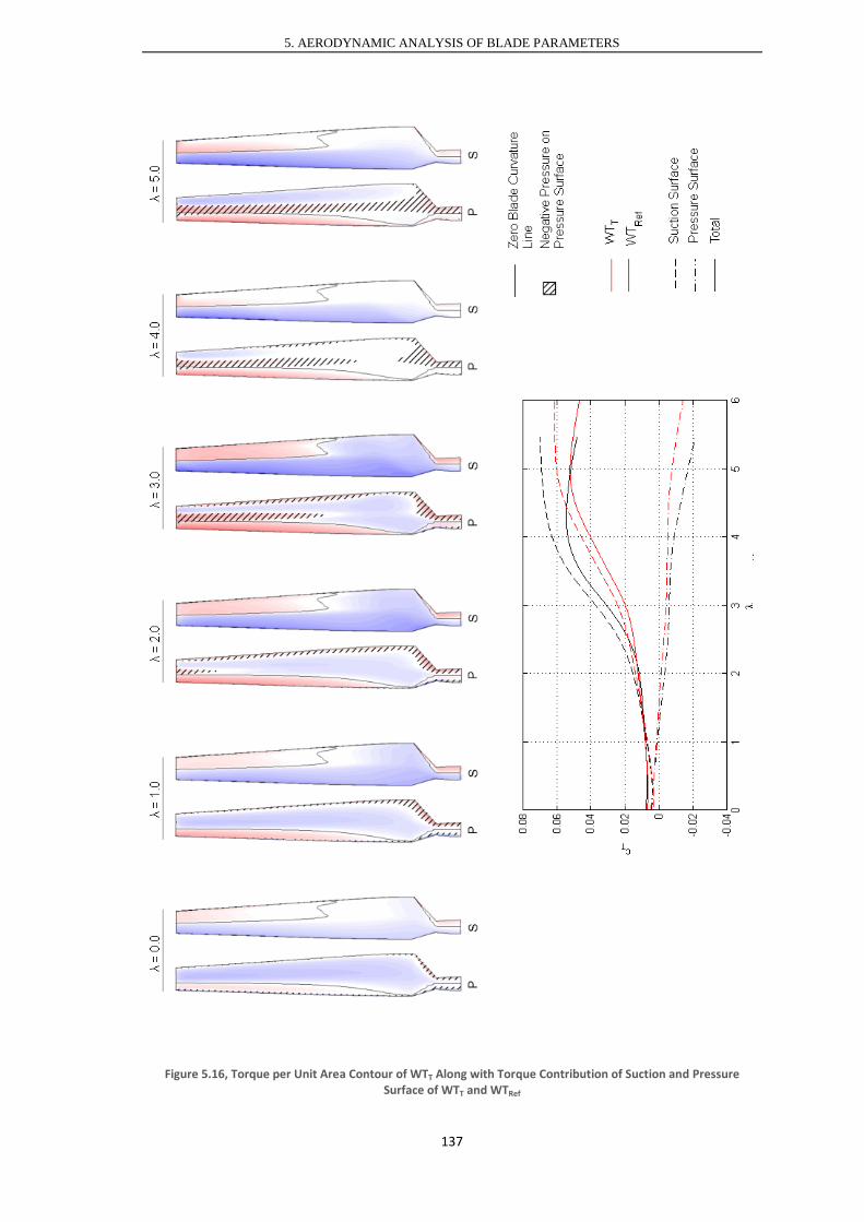
5. AERODYNAMIC ANALYSIS OF BLADE PARAMETERS
Figure 5.16, Torque per Unit Area Contour of WTT Along with Torque Contribution of Suction and Pressure Surface of WTT and WTRef
137

5. AERODYNAMIC ANALYSIS OF BLADE PARAMETERS
5.3.2 Flow Field at Reference Conditions
As there are no significant differences in cT between both blades at low λ, the following flow feature comparisons have been investigated at medium to high λ:
λT = 3.0 reveals information about the performance lack of the suction surface when reducing the blade thickness.
λT = 5.5 investigates the source of the larger attainable λ for the thin blade.
λT = 3.0
Figure 5.17 shows the flow structure on the suction surface and at cross sections r/R = 0.3, 0.6 and 0.9 for the thin blade and the reference blades operating at λ = 3.
Figure 5.17, Comparison of Flow Features of Blades with Thin (WTT) and Thick (WTRef) Profiles at λT = 3.0
The suction surface of the thin blade still experiences fully stalled flow whereas the reference blade only experiences partially attached flow for 0.7 < r/R < 1. The flow around the thin blade cannot attach to the blade as the higher blade curvature at the leading edge imposes a too high adverse pressure gradient. Consequently the upper half of the thinner
138

5. AERODYNAMIC ANALYSIS OF BLADE PARAMETERS
blade loses its torque producing capabilities and the thin blade draws a larger portion of its torque from the root than the reference blade. The increased blade curvature at the LE of the thinner blade is therefore responsible for the loss of the torque producing capabilities of the thin blade near the tip as observed in the radial torque graph in Figure 5.14. This loss leads to a delay of λ at which the suction surface experiences a high increase of cT with λT from ≈ 2.2 to ≈ 2.8 as can be seen in Figure 5.16.
Regardless of the chordwise extension of the flow separation bubble, the thin blade tends to produce thicker separation vortices. At r/R = 0.3 the sharp leading edge of the thin blade has caused the flow to form a LEV with a thickness of ≈ 0.13c close to the leading edge whereas the reference blade’s LEV only has a thickness of ≈ 0.04c at the same location. Both blades also show the formation of a very small TEV at r/R = 0.3 which significantly increases in size when approaching r/R = 0.6. At r/R = 0.6 the effect of the blade thickness is reduced and both blades produce an LEV of approximately 2.1 times the size of their TEV. At r/R = 0.9 the centre of the LEV of both blades has shifted towards the trailing edge, eliminating the TEV. The LEV of the thin blade however has a larger chordwise extension and thicker than that of the reference blade. This trend agrees with the relatively poor cT of the suction surface of the thin blade compared to the thicker blade’s suction surface as shown in Figure 5.16.
λT = 5.5
Figure 5.18, Comparison of Flow Features of Blades with Thin (WTT) and Thick (WTRef) Profiles at λT = 5.5
139

5. AERODYNAMIC ANALYSIS OF BLADE PARAMETERS
The streamlines of the flow around both turbines are presented in Figure 5.18. As it can be seen, the flow around both turbines is fully attached. Although the momentum of the flow has increased, the flow attachment can mainly be attributed to the reduction in α. It appears that the thin blade transitions from stalled flow to fully attached flow at a higher λ but within a shorter λ rang than the thicker blade. The lower gradient of cT with λT in Figure 5.16 for 3 < λ < 4.5 is therefore caused by a lower momentum extraction due to the lower aerofoil curvature towards the centre of the blade in the chordwise direction and by a slightly different pressure to torque translation.
5.3.3 Effect of Reynolds Number
This section investigates the role of blade thickness of turbines of different scales operating at different wind speeds. Figure 5.19 shows the cT and cP of WTRef and WTT at a 0.334m radius and a 5.029m radius operating at 3, 6 and 20m/s wind speed.
Figure 5.19, Power and Torque Performance of WTT in Comparison with WTRef at Turbine Scales 0.334m and 5.029m Radius Operating at 3, 6 and 20m/s
140

5. AERODYNAMIC ANALYSIS OF BLADE PARAMETERS
The cT of the stationary thin bladed turbine does not vary with vw or turbine radius. However, unlike for increasing blade pitched, reducing the blade thickness increases the design cP. The value of the maximum cP also depends on turbine scale and wind speed. As a result of reducing the blade thickness, the maximum cP performance of the large scale machine increases by 8, 7 and 6% when the turbine operates at a wind speed of 3, 6 and 20m/s respectively. This trend becomes even more severe for the scaled down turbine where a wind speed of 3, 6 and 20m/s is associated with a cP boost of 66, 21 and 9% respectively due to a blade thickness reduction.
Figure 5.20, Effect of Blade Thickness Comparing Total Torque Distribution of WTT with WTRef at Turbine Scales 0.334m and 5.029m, vw = 6m/s
Figure 5.20 presents an analysis evaluating the net torque differences when reducing the blade thickness from 0.21c to 0.15c at differently scaled turbines. The analysis has been conducted in a similar manner to that of the pitched turbine in section 5.2.3 and has been performed for vw = 3, 6 and 20m/s. Unlike for the pitched turbine, reducing the blade thickness is largely associated with a cT reduction. Due to the heavy flow stall at λ ≈ 0 and the following delay of the flow attachment for the thin blade as described in section 5.3.2, WTT experience a similar cT as WTRef over 0 ≤ λ < 2, irrespective of vw and turbine scale. This was only observed for λ up to 1.4 when pitching the blade. The following cT reduction of the large scale WTT is caused by a lower energy extraction due to the flatter blade centre. The effect of thickness of the large scale machine shows a moderate Re dependence while the small scale rotor shows a high Re dependence. At low vw the thickness effect even acts to almost exclusively favour the WTT’s cT performance over entire λ range, particularly from λT > 3.3. At a wind speed of 3m/s, the small turbine experiences a maximum Re of 23,000 when λ is in the range of 0 ≤ λ ≤ 4.6. Due to dominant viscous forces at ultra-low Re the flow is able to overcome the sharp LE of the thin blade much easier than at high Re where inertial forces dominate. When the flow has overcome the LE, the thin blade then promotes flow attachment due to its relatively low blade curvature in its chord-wise centre which only creates a weak adverse pressure gradient. The flow around the suction surface of the scaled down WTRef however is likely to separate due to the blade's higher curvature towards its chord-wise centre
141

5. AERODYNAMIC ANALYSIS OF BLADE PARAMETERS
and the adverse scaling effects which delay flow attachment as outlined in section 4.3.1. Consequently, when increasing vw the effect of the blade thickness of the small turbine approaches that of the large turbine. This is because it becomes increasingly more challenging for the flow around the thin blade’s LE to attach at a λ at which the flow around of the reference blade’s LE just begins to attach.
Figure 5.21, Effect of Blade Thickness Comparing Radial Torque Distribution of WTT with WTRef at Turbine Scales 0.334m and 5.029m, vw = 6m/s
A detailed analysis of the underlying torque change associated with reducing the blade thickness at different turbine scales is presented in Figure 5.21 for a wind speed of 6m/s. The interdependence between the blade thickness and Re effects has been evaluated by calculating the radial cT offset between WTRef and WTT. From λ ≈ 2 the cT performance of the analysed rotors begins to deviate noticeably as also suggested by Figure 5.19. The following radial torque reduction of WTT is initiated as α drops below 27° at the blade tip which has been discussed in great detail section 5.3.1. The radial torque drop of the large turbine is much more pronounced than that of the small turbine. This is because the large turbine operates in a nearly Re independent Re range. The performance of the thick bladed small turbine however is already limited by Re effects, the adverse blade reduction effects on cT when 15° < α < 27°, which occurs at moderate λ, are therefore less pronounced.
142

5. AERODYNAMIC ANALYSIS OF BLADE PARAMETERS
5.4 Combined Effect of Pitch and Thickness
In this section the effect of pitching a rotor blade of reduced thickness has been investigated. To allow for meaningful conclusions of the interaction between blade pitch and thickness, identical blade parameters to those investigated in the blade pitch study in section 5.2 and the blade thickness study in section 5.3, have been chosen for the new rotor design. The resulting blade is composed of the S809 aerofoil which has been reduced in its thickness from 21% to 15% and is pitched by 10° relative to the reference rotor.
The torque performance and flow features of the pitched, thin bladed turbine, WTP-T, have been analysed focusing on the effect of pitching the thin bladed turbine, WTT. This allowed a detailed study of the interaction between turbine pitch and thickness. The Reynolds number analysis however was conducted with respect to the reference turbine, WTRef, to enable the comparison between all turbine configurations investigated in chapter 5.
5.4.1 Torque Performance at Reference Conditions
Figure 5.22 shows the cP and cT performance of the pitched, thin bladed rotor along with the performance of the other 3 blade designs from λ = 0 up to each turbine’s respective design λ. All turbines had a radius of 5.029m and operated at a wind speed of 6m/s.
The pitched, thin bladed rotor reaches a maximum cP of 0.125 at λP-T = 3.44 which is 53% lower than the reference blade’s maximum cP. The corresponding cT of WTP-T is 0.0362. When the pitched, thin bladed turbine is stationary it produced a cT of 0.0135. This is only 1% lower than the cT of the thick pitched turbine, but is approximately twice the cT of the thick and thin un-pitched blades. This confirms the theory established in section 4.2 for WTRef and further developed in sections 5.2.1 and 5.3.1 for WTP and WTT respectively, that the torque of a stationary turbine is predominantly a function of the blade pitch, not a consequence of the aerodynamic profile or associated flow features.
Due to the cT trend of all turbine configurations the turbine behaviour of WTP-T was analysed from two aspects:
• The interaction between turbine pitch and blade thickness, whose isolated effect has been analysed in sections 5.2 and 5.3 respectively, was studied to relate the performance of the reference turbine to WTP-T.
• Further the effect of pitching a thin 0.15c blade and a thick 0.21c blade by 10° was investigated. This pitch analysis is also favoured by the practical aspect of the possibility of turbine pitch adjustment of small scale WTs, whereas blade thickness cannot be modified.
143

5. AERODYNAMIC ANALYSIS OF BLADE PARAMETERS
Figure 5.22, Power and Torque Performance of WTP-T and WTRef at 6m/s, Pitch and Thickness Interaction and Effect of Pitching Blades of Different Thicknesses at Radius 5.029m
The cT graph in Figure 5.22 illustrates the complex, nonlinear interaction between turbine pitch and blade thickness by comparing the actual cT difference between WTP-T and WTRef with that that would be obtained if the effect of both blade parameters was linear. For 0 ≤ λ < 1.54 the interaction produces a mild torque enhancement, following from 1.54 < λ < 2.71 the parameters interact to significantly reduce cT and thereafter they again enhance cT. If the parameters behaved linearly they would have produced an average cT improvement of 0.0079 with respect to the reference turbine over 0 ≤ λ ≤ 3.4. The actual cT behaviour of WTP-T however resulted in an average cT improvement of 0.0085 for the same λ range. This indicates that for the turbine configurations tested, WTP-T experiences an 8% cT enhancement due to nonlinear effects.
144

5. AERODYNAMIC ANALYSIS OF BLADE PARAMETERS
Figure 5.22 also shows that the λP-T – cT performance of the pitched, thin bladed turbine is relatively similar to that of the pitched thick bladed turbine, but not that of the reference turbine. This further confirms that the blade pitch angle primarily determines the turbine’s cT characteristics and that the blade thickness is only of secondary importance. Consequently, the effect of pitching rotor blades of different thicknesses has been investigated. Differences in the pitch investigations of the thick and thin blades are therefore caused by nonlinear blade pitch-thickness interactions described previously. The cT evolution with λ of both thin-bladed turbines occurs at a steadier rate than that of their thick-bladed counterparts. However there are some differences of how the effect of blade pitching is influenced by blade thickness. This is shown at the bottom of Figure 5.22 for the investigated blades. For 0 ≤ λ < 1.47 the thin blade benefits more from pitching than the thick blade. For 1.47 < λ < 2.52 however, the thick blade draws a higher benefit from operating in the pitched configuration. The thick blade’s performance enhancement peaks at 154% at λ = 2.15 as the cT of the 0.21c pitched turbine rapidly increases with λ at this rotational speed. The thin blade in contrast has a lower performance enhancement peak of only 124% at λ = 2.55 which is mainly due to the delay of λT at which cT rapidly increases with increasing rotational speed as described in section 5.3.1. On average however, the thin blade experiences a higher performance improvement of 95% when pitching the blade, while the thick blade’s performance is enhanced by only 89%. Based on the practical aspect of pitching turbine blades of different thicknesses, the following comparative torque studies have been conducted evaluating the effect of blade thickness on pitching:
Radial Torque Comparison
Blade Surface Torque Comparisons
Radial Torque Comparison
The effect of pitching a blade of 0.15c thickness by 10° on its normalised radial torque distribution has been investigated in this study and is illustrated in Figure 5.23. An equivalent study for the thick 0.21c blade is presented in Figure 5.3. The overall trend when pitching the thin blade follows that when pitching the thicker blade, differences have been identified as:
• The thick blade experiences the strongest shift of its torque production from the blade root to the blade tip when λ ≈ 2. The thin blade however experiences a less pronounced shift which is most prominent when λ ≈ 2.5. This is mainly caused by a more even radial torque distribution of WTP-T than WTP.
• After experiencing the pronounced shift of the torque producing blade segments, the thick and thin blades showed radial torque dependence on α. While the thick blade experienced an improved radial torque production when 11° < αP < 22° in the pitched configuration, the thin blade experienced a torque enhancement in the when 8° < αT-P < 18°. The cause for this has been investigated in the flow feature analysis.
145

5. AERODYNAMIC ANALYSIS OF BLADE PARAMETERS
Figure 5.23, Normalised Torque Distribution of WTT and WTP-T and Torque Differences Superimposed with Geometric α
Blade Surface Torque Comparisons
As the blade surface torque is determined by the flow features and the resulting pressure to torque translation which in turn is a function of the blade surface curvature, the blade surface gradients for WTP-T are illustrated in Figure 5.24. As expected, the surface curvature of WTP-T is similar to that of WTP shown in Figure 5.4. The pitched thin blade’s suction surface however is now better at translating negative pressure near its TE into useful torque than the pitched thick blade, whereas the pressure surface of the pitched thin blade has lost some of its good positive pressure to useful torque translation characteristics. The resulting torque per unit area contour plots of WTP-T are presented in Figure 5.25 along with the suction and pressure surfaces’ torque contribution of the thick and thin blade operating at βpitch = 10°. The equivalent graph for pitching a thick turbine blade is presented in Figure 5.5. Pitching a thin bladed turbine lowers the torque production of the suction surface throughout the entire λ range. The pressure surface experiences a slight cT drop for 0 ≤ λ < 0.12 which adversely affects turbine starting, but it produces a better cT for higher λ. The pressure surface
146

5. AERODYNAMIC ANALYSIS OF BLADE PARAMETERS
of WTP-T delivers the best cT performance of all turbine configurations tested and it is responsible for a higher design λP-T than λP.
Figure 5.24, Blade Curvature of Suction and Pressure Surface of WTP-T Along with Zero-Blade-Curvature-Line of WTP-T and WTRef
The torque per unit area contour plots of both blade surfaces of WTP-T and WTP show a similar pattern throughout the range of λ analysed. When the turbines are stationary, the torque per unit area of the pressure surface of WTP-T is slightly lower than that of its thicker counterpart. This results in a mild cT reduction of 3% and is a consequence of the thin pressure surface’s lower blade surface curvature, particularly in the root region. The thin blade’s suction surface experiences a similar cT loss.
When the blade operates at λ = 1, a 10° pitch of the reference blade has been associated with a pressure drop in the chord-wise direction below 0Pa on the pressure surface which resulted in a negative torque. This phenomena has not been observed when reducing the blade thickness in the βPitch = 0° position. Consequently the formation of negative torque on the pitched thin blade has been shifted to a higher λ. This is partly responsible for the extremely good performance of WTP-T’s pressure surface. Furthermore, the reduction of negative torque at the LE associated with reducing blade thickness of WTRef and with pitching WTRef, improves the cT performance of WTP-T. The suction surface of WTP-T and WTP show a very similar torque patter which explains their similar cT.
147

5. AERODYNAMIC ANALYSIS OF BLADE PARAMETERS
Figure 5.25, Torque per Unit Area Contour of WTP-T Along with Torque Contribution of Suction and Pressure Surface of Thin Bladed Rotor in Pitched (WTP-T) and Un-pitched (WTP) Configuration
When λ increases to 2, the suction surface of the pitched thin turbine however produces a 21% lower cT than its thick counterpart. This is caused by the absence of a strong suction peak which has been observed for the other 3 blade configurations. Although the cT of the pressure surface of WTP-T has dropped, the rotor continues to perform well compared to the other blades due to the mechanisms explained for λP-T = 1.
As the rotational blade speed increases further, the TE of the pitched, thin bladed rotor loses its torque producing ability except for at the blade root. The continuing cT production at the blade root is largely caused by a favourable pressure to torque translation in that region which is most pronounced for the WTP-T blade. The pressure surface of the investigated blade still produces a very favourable cT of ≈ 0 at λP-T = 3.
148
5. AERODYNAMIC ANALYSIS OF BLADE PARAMETERS
5.4.2 Flow Field at Reference Conditions
Based on the torque analysis of section 5.4.1, the flow features of the following λ have been analysed to gain a better understanding of the underlying flow features responsible for performance differences of WTRef, WTP, WTT and WTP-T. The analysis emphasis on understanding the role of pitching blades of different thicknesses as it may be possible to adjust the pitch angle of turbine blades but not the blade thickness.
λP-T = 2.0 reveals information about underlying flow features responsible for the higher cT enhancement when pitching the thick blade than when pitching the thin blade.
λP-T = 3.0 gives information on the more pronounced pitching induced cT enhancement of the thin blade than that of the thick blade.
λP-T = 2.0
The underlying flow features which contribute towards the higher cT improvement when pitching the thick blade than when pitching the thin blade, are analysed in Figure 5.26. The graph shows the flow on the suction surface of all 4 blade designs. The blades are subjected to large LEV’s covering most of their suction surfaces when they operate in the βpitch = 0° configuration. However when the blade pitch is increased to 10°, the flow around the tip of the 0.21c blade begins to attach, while the suction surface of the 0.15c blade is still almost exclusively covered by an LEV. Pitching the blades reduces α from 28° to 18° at r/R = 0.9. Although the geometrical Re of the flow approaching the thick and the thin blade is identical, the flow around the thick blade is able to remain attached to the blade tip due to the combination of a more favourable α at the blade tip and a less severe adverse pressure gradient imposed by the relatively large LE radius. The thick turbine blade shows two distinct stages as the flow transitions from fully separated to fully attached:
• Initially when the flow momentum is high enough to overcome the adverse pressure gradient at the LE, the flow attaches from 0 ≤ c < 0.45. This is occurs for 0.8 < r/R < 0.9 in Figure 5.26. Further radially inwards the bade typically shows a relatively long transition period where the flow separation line moves from c ≈ 0.45 to the leading edge as the momentum of the flow decreases.
• When moving radially outwards from the partially attached flow the flow undergoes a rapid transition within a short radial distance to become fully attached.
More examples visualising both flow regimes of the thick blade are shown in Figure 5.9 for λ = 3 where it operates in the pitched position and in Figure 4.8 for λ = 4. Figure 4.9 depicts λ = 1 to 6 when the blade operates in the un-pitched configuration, i.e. WTRef.
149

5. AERODYNAMIC ANALYSIS OF BLADE PARAMETERS
Figure 5.26, Streamlines on Suction Surfaces of WTRef, WTT, WTP and WTP-T at λ = 2
λP-T = 3.0
When the analysed blades rotate at a higher rotational speed of λ = 3.0, the increase of the momentum of the air approaching the rotor is responsible for larger areas of the blades suction surfaces being covered by fully or partially attached flow as shown in Figure 5.27. The flow attachment mechanism for the thick blade described for λ = 2.0, is responsible for 0 < r/R < 0.65 of the pitched, thick blade operating in partially stalled flow and 0.65 < r/R ≤ 1 experiencing fully attached flow. The suction surface flow pattern of the thick blade operating in the βpitch = 0° at λRef = 3 is similar to that of the thick, pitched blade operating at λP = 2.
Figure 5.27 shows that the thin blade only undergoes a single stage flow attachment mechanism unlike the thick blade. Due to the increased adverse pressure gradient imposed by the smaller LE radius of the thin blade, the thin blade requires a higher flow momentum for the flow to attach. This has been explained in detail in section 5.3.2. The following flatter aerofoil cross sectional shape of the thin blade means that once the flow has overcome the sharp LE of the 0.15c blade, it is more likely to remain attached than when flowing past the 0.21c blade. This is due to the lower adverse pressure gradient at the 0.15c blade’s centre in the chord-wise direction. Figure 5.27 also shows the cross sectional streamline pattern of WTP-T at r/R = 0.3, 0.6 and 0.9 to allow for a more detailed flow feature comparison with the
150

5. AERODYNAMIC ANALYSIS OF BLADE PARAMETERS
other blades. The corresponding cross sectional flows at λ = 3.0 of WTRef and WTP are shown in Figure 5.9 and that of WTT is illustrated in Figure 5.17. At r/R = 0.9 the un-pitched thick blade shows a much smaller LEV than the un-pitched thin blade. Upon pitching however both blades’ LEV disappears. This further confirms the high pitching effectiveness of the thin blade for λ =3. Towards the blade root when r/R ≤ 0.6 both, the thick and the thin un-pitched blades show comparable LEV and TEV sizes. Upon pitching each blade’s TEV vanishes completely, but the LEV of the pitched, thin blade tends to be slightly larger than that of the thick blade.
Figure 5.27, Streamlines on Suction Surfaces of WTRef, WTT, WTP and WTP-T and Cross-Sectional Flow of WTP-T at r/R = 0.3, 0.6 and 0.9 at λ = 3
The different flow attachment process of the thin and the thick blade is mainly responsible for the different pitching effectiveness of the thin and the thick blades. The high pitching effectiveness at λ𝑜𝑜𝑏𝑏=0.21𝑐𝑐 = 2.15 of the thick blade is caused by the attachment of the flow when the blade is pitched. At the same rotational speed the pitching effectiveness of the thin blade does not increase significantly as its suction surface still largely operates in fully stalled flow even when it is pitched. When increasing λ however the flow around the thin blade begins to rapidly attach which leads to the thin blade’s pitching peak at λ𝑜𝑜𝑏𝑏=0.15𝑐𝑐 = 2.55.
151

5. AERODYNAMIC ANALYSIS OF BLADE PARAMETERS
5.4.3 Effect of Reynolds Number
In this section the role of the interaction of the combined pitch and thickness effect with varying wind speed and turbine scale has been evaluated. Figure 5.28 shows the cP and cT evolution of WTRef and WTP-T at a 0.0334m and a 5.029m scale, operating at wind speeds of 3, 6 and 20m/s. The equivalent graphs showing the isolated effects of pitch and blade thickness are shown in Figure 5.10 and Figure 5.19 respectively. The cT – λ curves of the pitched thin bladed rotor are dominated by the effect blade pitch, not by the effects of blade thickness. The maximum cP of WTP-T is also dominated by effects from WTP, not from WTT. The large scale WTP-T experiences a cP loss of 53% with respect to the reference turbine which is independent of vw. Scaling WTP-T down introduces wind speed dependence. Wind speeds of 3, 6 and 20m/s are associated with a cP decrease of 27, 47 and 51% respectively. Table 5.1 summarises the cP enhancement or reduction of all turbines analysed with respect to WTRef at different wind speeds.
Figure 5.28, Power and Torque Performance of WTP-T in Comparison with WTRef at Turbine Scales 0.334m and 5.029m Radius Operating at 3, 6 and 20m/s
152

5. AERODYNAMIC ANALYSIS OF BLADE PARAMETERS
vw [m/s] Full Scale Small Scale
WTP WTT WTP-T WTP WTT WTP-T 3 -51 +8 -53 -51 +66 -27 6 -51 +7 -53 -55 +21 -47 20 -51 +6 -53 -48 +9 -51
Table 5.1, Percentage Change of Maximum cP of WTP, WTT and WTP-T with Respect to WTRef at Different Wind Speeds [%]
The combined effect of pitch and reduced thickness has been analysed with respect to the reference turbine in Figure 5.29 and Figure 5.30. The cT performance of WTP-T has been analysed while considering the isolated effects of pitching and reducing blade thickness which have been visualised in Figure 5.11 and Figure 5.12 for WTP as well as in Figure 5.20 and Figure 5.21 for WTT. The net cT enhancement of WTP-T with respect to WTRef is illustrated in Figure 5.29. The large scale pitched, thin bladed rotor is adversely affected by the blade thickness reduction as it shows a significantly lower cT improvement than the pitched turbine. For increasing vw its cT improvement also decreases which is also a trait of the thin bladed turbine. The small scale turbine however highly benefits from the combined effect of pitch and blade thickness. At a low wind speeds the reduction of α enhances the viscous force driven flow attachment around the blade’s sharp LE and thereby increase the cT enhancement nonlinearly. At λ = 2.5 the small scale pitched turbine produced a cT enhancement of 0.009 when vw = 3m/s, while the thin bladed turbine produced a very lower cT improvement of 0.001 but the pitched, thin bladed rotor produced a cT enhancement of 0.013 at the same wind speed. Although the cT improvement of WTP-T continues to rise for increasing vw, the nonlinear share of the increase goes down. This is because the cT enhancement from blade thickness effects of the small scale WTT or WTP-T results from viscous forces which become less dominant with increasing vw. Nonetheless, at a wind speed of 20m/s the small scale WTP-T almost exclusively outperforms the cT improvement of the large rotor.
Figure 5.29, Effect of Blade Pitch and Blade Thickness Comparing Total Torque Distribution of WTP-T with WTRef at Turbine Scales 0.334m and 5.029m at vw = 6m/s
153

5. AERODYNAMIC ANALYSIS OF BLADE PARAMETERS
In Figure 5.30 the combined effect of pitch and thickness on the radial cT distribution has been evaluated with respect to WTRef for both turbine scales. At a wind speed of 6m/s, the change of the radial torque distribution between WTP-T and WTRef is dominated by the change associated between WTP and WTRef for the large and small turbine scale. The slightly lower cT improvement of WTP-T with respect to WTRef than that of WTP with respect to WTRef in the range of 10° < α < 20° for is undoubtedly caused by the significant cT reduction at a similar α range when only reducing the blade’s thickness. This pitch – blade thickness interaction is more pronounced for the large scale rotor than for the small rotor.
Figure 5.30, Effect of Blade Pitch and Blade Thickness Comparing Radial Torque Distribution of WTP-T with WTRef at Turbine Scales 0.334m and 5.029m Operating at 6m/s
5.5 Applicability of Lower Order BEM Methods
In this section the applicability of lower order BEM methods to accurately reflect the effect of blade thickness and blade pitch has been investigated. Hereby the emphasis was placed on the effect of the non-linear interaction of blade thickness and blade pitch when they are applied together which has been observed in section 5.4. The capability of BEM calculations to reflect these nonlinearities depends on the BEM code itself as well as the quality of the aerodynamic input data used for the BEM code.
154
5. AERODYNAMIC ANALYSIS OF BLADE PARAMETERS
5.5.1 Comparison between BEM Assumptions and CFD Results
During the derivation of BEM codes, several assumptions are made as outlined in section 2.5.2. A key assumption is that there are no interactions between the radially discretised elements along which the aerodynamic cL and cD forces are resolved. However the CFD analysis of the different blades in chapter 4 and in sections 5.2 through 5.4 has shown that there is a significant amount of cross flow in regions where the flow is separated which occurs at low λ. The streamlines of all blade configurations have been displayed in Figure 5.26 and Figure 5.27 for a λ of 2 and 3 respectively. There is a strong radial cross flow for all blades at λ = 2, nonetheless the streamline patterns are relatively similar. At λ = 3 however the streamline patterns of all blades indicate that the blades exhibit a different flow attachment behaviour. Not only do the areas over which the flow is separated vary, the magnitude and direction of the separated flows are also different. BEM codes are thus not able to directly model nonlinear pitch thickness interactions due to their inherent assumptions. However, the aerodynamic input data which is used by the code may be modified in an attempt to account for the effect of the cross flow on cL and cD.
5.5.2 BEM Input Data
The aerodynamic input data for the BEM code used to calculate turbine performance has to be of high quality in order to resolve nonlinear pitch-thickness interactions. In this thesis aerodynamic data accounting for angle of attack ranges from ≈ -2° to up to 90° and Re effects are required. Additionally the aerodynamic input data may be modified in an attempt to account for the effect of radial cross flow which is particularly important for low λ as outlined in section 5.5.1. The aerodynamic data itself however may be derived experimentally or computationally.
Publically available experimental lift and drag data is typically only available for common aerofoil series such as the NACA series which already limits the number of blade designs that can be analysed. Furthermore for a given profile the aerofoil has usually only been analysed over a narrow α range at no more than a few Re numbers. Because of this, approximations for cL and cD, such as the use of the flat plate equation at high α, are often made. Increasing experimental uncertainty for flows at high α and low Re make the derivation of accurate cL and cD in this range difficult.
To overcome these problems computationally derived aerofoil performance data may be used. Programmes which are based on potential flow theory, such as XFOIL which has originally been written in 1986, allow the simulation of arbitrary shapes. Following is a brief analysis of the capability of potential flow theory to deliver high quality cL and cD coefficients for the use in BEM computations for turbine start-up. When assuming irrotational as well as incompressible flow, the flat plate’s lift equation which is shown in Equation 5.2 can be derived using potential flow theory. The equation has been derived by superimposing the flow solutions of a flat plate that is placed parallel to the incoming flow, a flat plat that is placed perpendicular to the incoming flow as well as the Kutta condition which ensures that the flow smoothly leaves the trailing edge of the flat plate. Schlichting and Truckenbrodt [98] have
155

5. AERODYNAMIC ANALYSIS OF BLADE PARAMETERS
extended the potential flow analysis to account for the effect of profile thickness using the Joukowsky profile which is a thin, symmetrical aerofoil. The resulting aerofoil thickness and pitch relation for cL is given in Equation 5.3.
𝑐𝑐𝐿𝐿 = 2𝜌𝜌 sin𝑑𝑑 Equation 5.2 𝑐𝑐𝐿𝐿 = 2𝜌𝜌(1 + 0.77𝑡𝑡𝑏𝑏) sin𝑑𝑑 Equation 5.3
Equation 5.3 indicates that α has a greater effect on cL than tb. It furthermore shows that the lift slope of the Joukowsky aerofoil increases with increasing thickness. Reducing the thickness of the aerofoil from 0.21 to 0.15c is accompanied by a 4% reduction of its lift slope. These findings however have to be treated with care as they are derived from potential flow theory and are thus not applicable in situations where viscous effects are of primary importance such as in separated flows around aerofoils or turbine blades. Differences between experimental investigations and calculations based on potential flow theory have been observed to be small only in regions where the boundary layer is thin and the drag is low. Outside this region it is advisable to use experimental data [99].
It is thus unlikely that lift and drag data obtained experimentally or computationally using methods based on potential flow theory are of high enough quality to accurately model nonlinear pitch thickness interactions. Both approaches tend to have increasing difficulties in accurately predicting cL and cD at flows with high α which corresponds to λ for HAWTs. When also considering the lack of the cross flow in BEM which has been described in section 5.5.1, it seems unlikely that BEM methods are able to accurately model the observed nonlinear blade pitch and thickness interactions in this thesis. The BEM limitations however are removed when using 3D CFD to model complete wind turbine blades.
5.6 Summary
In this section the performance of 3 blade configurations has been compared to that of the reference turbine at a turbine scale of 5.029m and a wind speed of 6m/s. The turbines performance, their torque characteristics and flow features have been analysed in detail. Reynolds number effects of each blade design were evaluated at turbine radii 0.334m and 5.029m and wind speeds of 3, 6 and 20m/s. Additionally the suitability of blade element momentum methods has been assessed to reproduce the results observed during computational fluid dynamics computations in order to place the research conducted into a wider body of knowledge.
156

5. AERODYNAMIC ANALYSIS OF BLADE PARAMETERS
Blade Pitch: 0° Increased to 10°
• The greatly improved cT performance of the pitched blade is the result of a more favourable pressure-to-torque translation and more favourable flow features which act to significantly increase the torque contribution of the blade tip.
• The flow features at a given radial location and λ of the pitched turbine are bound by those encountered by the un-pitched turbine operating at the same λ and the un-pitched turbine operating at a higher λ to match α at the given radial location. At low λ the pitched turbine operates closer to the lower boundary and at high λ closer to the upper boundary.
• The pitched blade’s optimum cP of 0.127 is limited by its low design λ of 3.2 which is due to the poor cT performance of the pressure surface. At higher λ the blade tip begins to operate at α < 9° and thus generates a too low cT.
Reynolds number effects:
• Pitching the blade reduces the maximum attainable cP by ≈ 50% regardless of turbine scale or wind speed.
• At low wind speeds nonlinear effects between blade pitch and turbine scale significantly reduce the pitching enhancement of the small rotor but not that of the large rotor. This is a consequence of adverse Re effects at low Re when 10° < α < 20°.
Blade Thickness: 21% Reduced to 15%
• When 0 < λ < 2 the cT and cP performance of the thick and thin bladed turbine is similar as both blades operate in fully stalled flow.
• The flow around the suction surface of the thin blade requires a reduction of α from 22° to 19° along with a higher flow momentum to overcome the increased adverse pressure gradient from the higher blade curvature at the leading edge. This causes a delay in λ at which cT rapidly increases with λ from 2.2 to 2.8
• The following increase of the suction surface’s cT with λ occurs at a lower rate as the blade cannot extract as much energy from the flow due to its lower surface curvature towards the blade centre in the chordwise direction.
• The pressure surface benefits from the reduced blade thickness and generates less negative cT which is largely responsible for the improved cP performance of the thin blade which with cP = 0.280 is 7% higher than that of the reference blade.
Reynolds number effects:
• Reducing the blade thickness increases the maximum attainable cP compared to the reference blade. Turbines operating at lower wind speeds benefit from a thinner blade, especially small scale machines.
• The full scale rotor loses some of its cT performance when reducing its thickness due to the delay in flow attachment. The smaller rotor however benefits from a thinner
157

5. AERODYNAMIC ANALYSIS OF BLADE PARAMETERS
blade at low wind speeds as viscous forces support flow attachment over the blade’s sharp leading edge at very low Re.
Combined Blade Pitch and Thickness: 10° Pitch and 15% Thickness
• On average the 0.15c thickness blade experiences a higher cT enhancement due to pitching than the 0.21c blade. The thin, pitched blade however experiences its highest cT enhancement at a higher λ than the thick blade. This is caused by a shift of the flow attachment of WTP-T towards a higher λ which occurs over a shorter λ span.
• The cT and the corresponding surface torque distribution of WTP-T are dominated by pitching effects rather than blade thickness effects. The pressure surface of WTP-T however particularly benefits from the performance enhancing cT effects when pitching the reference blade and reducing its thickness.
Reynolds number effects:
• The large scale WTP-T experiences a cP loss of 53% with respect to the reference rotor. Small scale turbines experience a lower loss which further decreases with decreasing wind speed.
• The large scale machine is adversely affected by the combined blade thickness and pitch effects. The small rotor however produces a nonlinear cT improvement at low wind speeds due to the thin blade’s beneficial low Re effects.
Suitability of Blade Element Momentum Methods
The accuracy of blade element momentum methods is influenced by assumptions made during the derivation of the code and the quality of the aerodynamic input data. Limitations associated with both aspects make it unlikely that BEM is capable of reproducing the blade pitch and thickness effects observed during CFD computations:
• The CFD investigations have shown that all blades analysed experience radial cross flow at very low λ. As λ ≈ 3 the size and strength of the recirculation bubble on the suction surface becomes furthermore dependent on the turbine pitch and blade thickness. This obstructs an accurate representation of the aerodynamics through BEM methods as they assume no interaction between different radial blade segments.
• Aerodynamic input data for BEM codes derived using experiments or codes based on potential flow theory are prone to inaccuracies at high α which corresponds to a low λ turbine operating condition.
158

6. WIND TURBINE STARTING
6.1 Introduction
To date no systematic studies on the role of turbine starting on energy yield have been conducted, although small scale rotors face several unique power reducing issues as outlined in chapter 1. In this chapter a detailed analysis that addresses the understanding of turbine starting and quantifies the effect of the rotor geometry on energy yield, has been presented. Different turbine radii and wind speeds have been considered. The rotor geometries correspond to the turbines whose steady state performance has already been investigated in chapter 4 and 5, namely the reference rotor, a rotor with a reduced blade thickness from 21% to 15%, a rotor with increased blade pitch from 0 to 10° and a rotor with both, reduced blade thickness and increased pitch. Turbine radii of 0.334 and 5.029m were analysed to investigate the effect of turbine scale in combination with a wind speed range from 3 to 20m/s. Turbine starting has been simulated using the quasi-steady state method which has been validated in chapter 3.
Section 6.2 focuses on the influence of the torque and flow features produced at different λ of all four blade designs, as the blades accelerate from rest to full operational speed. It is the aim of this section to put the radial torque and flow features that have been identified in previous chapters into perspective with respect to the turbines starting performance rather than to introduce new analysing concepts. The relevance of the evaluated starting sequence has then been investigated with respect to the energy yield in section 6.3 as the turbines are subjected to gusts of different strengths and lengths. Such systematic studies not only investigating the underlying flow and torque phenomena of the effect of blade pitch, thickness and combined pitch and thickness, but also their effect on the energy yield have not

6. WIND TURBINE STARTING
been conducted before. References to the literature presented in chapter 2 were made to establish agreements and disagreements with other researchers as well as to highlight new findings of this thesis.
Throughout this chapter the following assumptions have been made:
• The turbine blades are stiff enough to not deform or deflect. This assumption has been commonly made in literature for small scale HAWTs.
• The wind approaches the turbine perpendicular to its rotational plane and wind speed and direction do not change during a gust.
• The generator does not exert resistive torque on the turbine. Accounting for the resistive torque would elongate the starting sequence as suggested by section 2.4.1, typical values for TRes are given in Table 2.3. The generator only engages when the rotor has reached the λ corresponding to its maximum cP. During turbine starting the entire aerodynamic torque is therefore used to accelerate the turbine to its full operational speed.
• The change in blade inertia due to pitching is insignificant but the inertia scales linearly with blade thickness, see Equation 2.6. The turbine inertia of the full scale WTRef was taken from the NREL Phase VI experimental measurements and that of the small scale rotor was measured from the small scale turbine blade model at the University of Sheffield. Resulting turbine inertias are shown in Table 6.1.
R = 5.029m R = 0.334m WTRef , WTP 949 4.5 x 10⁻³ WTT, WTP-T 678 3.2 x 10⁻³
Table 6.1, Turbine Inertia of All Analysed Rotors [kgm2]
6.2 Typical Starting Sequences
It is the aim of this section to investigate typical starting sequences of all 4 two-bladed rotors that have been introduced in chapters 4 and 5 when they accelerate from rest to their respective design λ. The main focus hereby lies on identifying the relative importance of different torque and flow features on the starting sequence, not on introducing new concepts for their analysis. By doing so, design features facilitating or impeding different stages of the starting sequence and the overall turbine start were identified. Such a detailed turbine starting analysis is the first of its kind to the author’s knowledge.
160

6. WIND TURBINE STARTING
6.2.1 Reference Blade
The starting performance of the full scale two-bladed reference turbine has been investigated as it is subjected to a wind speed of 6m/s. The net turbine torque at different λ and its impact on the turbine start-up as well as the underlying radial torque distribution have been analysed. Significant λ for WTRef derived in chapter 4 are summarised in Table 6.2 along with the time at which they are encountered during starting.
Stage λ Time [s] Description Start 0.00 0.0 WT begins to rotate, Re at the root is larger than at the tip
1 1.97 32.2 The local Re is nearly uniform along the blade span causing the dominant torque production to start to shift from the blade root to the tip
2 2.48 37.0 α at the blade tip drops below 22°, the cT production begins to significantly increase
3 4.25 43.6 Maximum cT as the entire blade experiences α below 22°. The pressure surface begins to experience a higher cT reduction than the cT increase of the suction surface, causing a net cT reduction
End 5.50 46.6 Maximum cP, generator is engaged
Table 6.2, Significant λ’s of WTRef Along with the Time at which They Occur During Turbine Starting at 6m/s, R = 5.029m
Figure 6.1 shows the rotational blade motion derivatives in their dimensional and non-dimensional form as the turbine accelerates along with stages 1 to 3 as outlined in Table 6.2. The stationary turbine experiences a cT of 0.0075 which causes it to accelerate at 0.070 rad/s2. This low turbine torque and acceleration is maintained for approximately 35s. It denotes the idling period which is described in section 2.4.1 and has been observed by several researchers such as Wright and Wood [48]. The end of the idling period is initiated when Re at the tip rises above that of the blade root as stated in stage 2. Approximately 69% of the starting time is required for this to occur. The following phase during which the turbine accelerates rapidly until it reaches full operational speed has also been observed in literature. However the detailed acceleration characteristics that have been presented in this thesis could not be measured experimentally. The turbine acceleration begins to increase most rapidly as an increasing portion of the blade operates at α < 22°, until the entire blade experiences α < 22° which is denoted stage 3. This phase only lasts for 14% of the total starting time. The turbine acceleration peaks at 0.50rad/s2 at time 44s. Afterwards the turbine’s acceleration reduces to 0.45 rad/s2 when the turbine reaches its maximum cP of 0.26. At the time of power extraction the rotor acceleration drops to zero. The starting sequence lasts for 46.6s in total and requires 7.42 turbine revolutions.
161
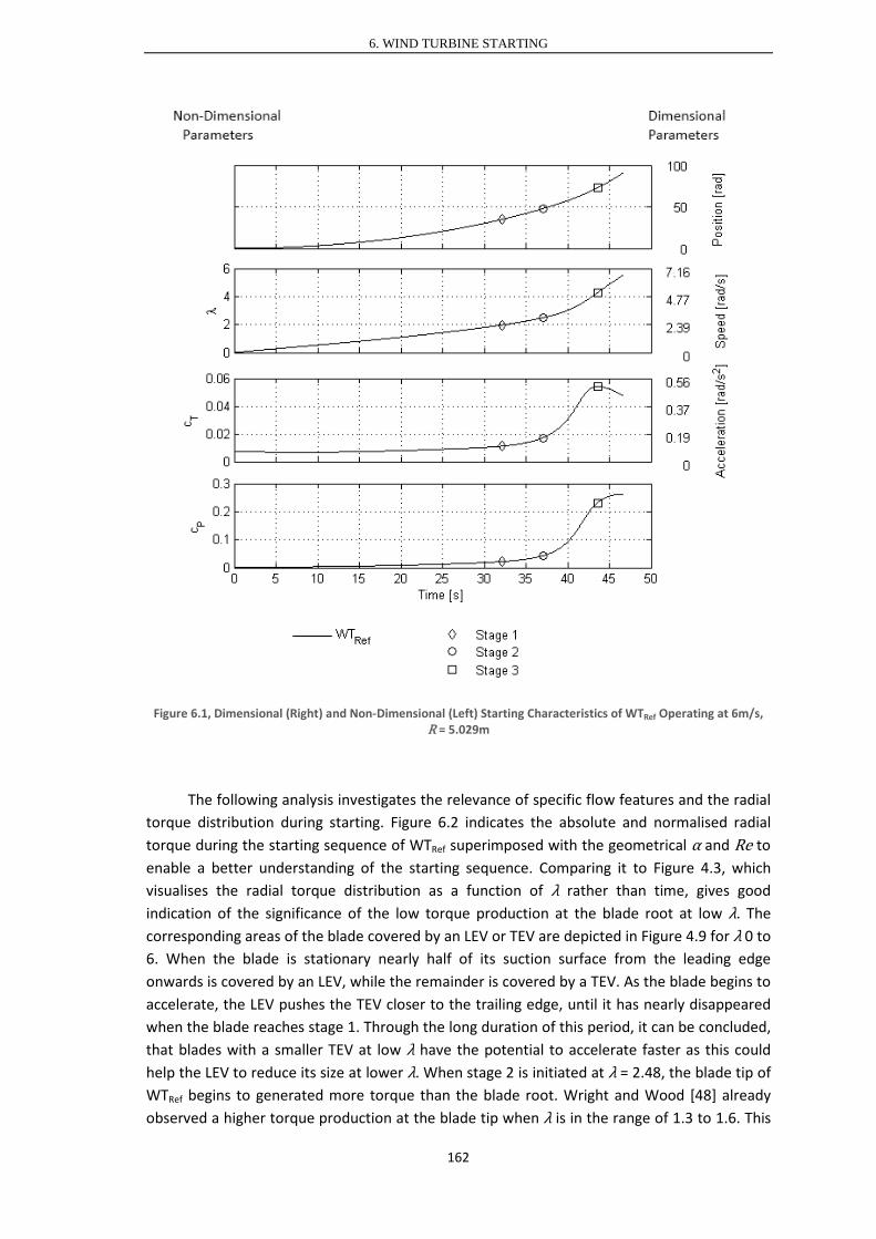
6. WIND TURBINE STARTING
Figure 6.1, Dimensional (Right) and Non-Dimensional (Left) Starting Characteristics of WTRef Operating at 6m/s, R = 5.029m
The following analysis investigates the relevance of specific flow features and the radial torque distribution during starting. Figure 6.2 indicates the absolute and normalised radial torque during the starting sequence of WTRef superimposed with the geometrical α and Re to enable a better understanding of the starting sequence. Comparing it to Figure 4.3, which visualises the radial torque distribution as a function of λ rather than time, gives good indication of the significance of the low torque production at the blade root at low λ. The corresponding areas of the blade covered by an LEV or TEV are depicted in Figure 4.9 for λ 0 to 6. When the blade is stationary nearly half of its suction surface from the leading edge onwards is covered by an LEV, while the remainder is covered by a TEV. As the blade begins to accelerate, the LEV pushes the TEV closer to the trailing edge, until it has nearly disappeared when the blade reaches stage 1. Through the long duration of this period, it can be concluded, that blades with a smaller TEV at low λ have the potential to accelerate faster as this could help the LEV to reduce its size at lower λ. When stage 2 is initiated at λ = 2.48, the blade tip of WTRef begins to generated more torque than the blade root. Wright and Wood [48] already observed a higher torque production at the blade tip when λ is in the range of 1.3 to 1.6. This
162

6. WIND TURBINE STARTING
difference will be caused by the use of different blade profiles with different cT vs. α and Re characteristics as well as experimental uncertainties. After the turbine has passed stage 2, the flow begins to attach to the blade as the LEV begins to both, reduce its thickness and its extent along the suction surface. When reaching stage 3, the flow along the entire blade span is at least partially attached onto the suction surface. While α along the blade only slowly decreases in time, a rapid increase of the radial Re has been observed from stage 3 onwards as seen in Figure 6.2. This also aids a high cT production when completing the rotor start-up.
Figure 6.2, Absolute and Normalised Radial Torque Distribution During Turbine Starting of WTRef, WTP, WTT and WTP-T Operating at 6m/s, R = 5.029m
6.2.2 Effect of Blade Geometry
The influence of modifying the reference turbine’s geometry has been observed in chapter 5 with respect to the turbines steady λ performance. In this section, the impact of altering the rotor geometry with respect to the rotors’ self-starting properties has been evaluated. Figure 6.3 shows the non-dimensional starting derivatives of all 4 full scale WTs. All turbines were observed to first undergo an idling period and then rapidly accelerate to their final operating speed. WTRef requires the longest starting time while that of WTT, WTP and WTP-
T has been reduced by 22, 55 and 66% respectively as a consequence of modified aerodynamics, blade surface curvatures and turbine inertia as outlined in Table 6.1. The
163

6. WIND TURBINE STARTING
corresponding λ at which stages 1 to 3 occur are shown in Table 6.3. The dominant effect of pitching a rotor blade and the secondary nature of the blade thickness effect observed in chapter 5, are also reflected in the turbines starting behaviour. The remainder of this section investigates the turbines starting characteristics in more detail with the following focus:
Turbine Pitch Turbine Thickness
Figure 6.3, Non-Dimensional Starting Characteristics of WTRef, WTP, WTT and WTP-T Operating at 6m/s, R = 5.029m
Stage WTRef WTP WTT WTP-T 1 1.97 1.97 1.97 1.97
2 f(α)
2.48 (αTip < 22°, see
Figure 4.3)
1.60 (αTip < 22°, see
Figure 5.3)
2.90 (αTip < 19°, see
Figure 5.14)
1.80 (αTip < 19°, see
Figure 5.23) 3
f(α) 4.25
(αBlade < 22°) 3.00
(αBlade < 22°) 4.74
(αBlade < 19°) 3.32
(αBlade < 19°)
Table 6.3, λ at which Stages 1-3 from Table 6.2 Occur for WTRef, WTP, WTT and WTP-T
164

6. WIND TURBINE STARTING
In order to relate the instantaneous cT generation to the turbine starting time a relationship has been derived based on the quasi-steady turbine starting modelling approach which has been validated in section 3.3.4. Equation 6.1 has been derived by substituting Equation 2.3 into Equation 2.9. It indicates that cT is inversely related to the starting time which has been visualised for all WT blades in Figure 6.4.
𝑑𝑑𝑡𝑡 =2𝐼𝐼
𝜌𝜌𝜌𝜌𝑅𝑅3𝑣𝑣𝑤𝑤2
1𝑐𝑐𝑇𝑇
𝑑𝑑𝑅𝑅 Equation 6.1
Figure 6.4, cT Contribution towards Starting Time for WTRef, WTP, WTT and WTP-T at vw = 6m/s, R = 5.029m
Turbine Pitch
The observed effect of pitching turbine blades in this thesis follows the trend observed in literature which is shown in Figure 2.18. When pitching the full scale reference turbine, the starting time is reduced due to the high increase in cT of approximately 79% when the pitched rotor is stationary. This significant increase is caused by a more favourable pressure to torque translation of WTP due to the modified angle of the blade surface with respect to the rotational plane, rather than by significant changes in flow features as described in detail in section 5.2.2. It acts to considerably speed up turbine starting as it can be seen in Figure 6.3 and Figure 6.4.
After rotation has been initiated, a slight drop in cT, which is more pronounced for the un-pitched turbines, significantly elongates turbine starting. The drop is caused by a too low increase of the cT production of the suction surface to compensate the drop in cT of the pressure surface up until λ ≈ 0.25. This is described in detail in section 4.2.1 and 5.2.1 for WTRef and WTP respectively. Table 6.3 indicates that both turbines, WTRef and WTP, begin to produce a rapidly increasing radial cT when αTip < 22°, denoted stage 2. Due to the pitching angle difference of 10° between both turbines, stage 2 is shifted from λ = 2.48 for WTRef to λ = 1.60 for WTP. This shift causes a reversed order of stage 1 and stage 2 for WTP, as λ at which stage 1 occurs does not change due to its sole dependence on the chord distribution which has not been modified in this thesis. The earlier occurrence of stage 2 for the pitched turbines causes
165

6. WIND TURBINE STARTING
the rapid blade acceleration to be initiated from time 14.8s for WTP instead of at time 37.0s for WTRef. This rapid acceleration is caused by an LEV of a reduced thickness and extent for WTP compared to WTRef which is shown in Figure 5.8 for λ = 1.5. The TEV has been pushed back right to the trailing edge and nearly disappeared at this λ.
When WTP then reaches stage 1 at time 16.9s, no noticeable effect of the turbine acceleration was observed which emphasises on the secondary importance of the Re distribution compared to the α distribution. The WTP reaches its optimum cT 3.2s later when αBlade < 22° at time 20.1s and finishes the starting sequence at time 21.1s.
Turbine Thickness
Reducing the blade thickness acts to reduce the blade’s starting time which has also been observed by Worasinchai [31], see Figure 2.21. The reduction of the blade thickness from 21 to 15% is accompanied by an inertia reduction of 29% due to the assumed linear relation between blade thickness and inertia in Equation 2.6. This in turn is responsible for a 29% decrease of the starting time of the thin blades as the starting time scales linearly with blade inertia as shown in Equation 6.1 when there is no resistive torque. In the un-pitched configuration the turbine however only experiences a 22% reduction of its starting time while with a 10° pitch angle the starting time is reduced by 24% due to blade thickness effects. This is shown in Figure 6.3. The relative underachievement can therefore be attributed to aerodynamic effects. This non-linearity between blade thickness and pitch has been analysed in detail in section 5.4.
Due to the high α and the high blade curvature at the LE, the 0.15c blade only produces a cT of 0.0068 in the un-pitched configuration when it is stationary which is then followed by a drop in cT when λ < 0.3 as can be seen in Figure 5.13. This drop is less pronounced for the pitched thin bladed turbine as shown in Figure 5.22 as the flow experiences a more favourable α. This leads to the formation of relatively similar vortices at the suction surface of WTP and WTP-T. The high significance of the comparatively low cT production on the starting performance of the un-pitched rotors is visualised in Figure 6.4. Reducing the blade thickness of the un-pitched rotor is accompanied by a reduction in cT when λ < 0.78 which has not been observed when varying blade thickness in the pitched blade configuration. This is largely responsible for the lower reduction of the turbine starting time for WTT than for WTP-T.
The reduction of the blade thickness from 21 to 15% is accompanied by reduction of α at which a high increase of the blade’s radial cT is observed, from 21° to 19°, independently of the blade’s pitch angle. This is caused by the formation of a smaller LEV as shown in Figure 5.17 as the flow of the thin blade is subjected to a lower adverse pressure once it has overcome the sharp leading edge which has been discussed in detail in section 5.3 and 5.4. The reduction of the performance enhancing α of the thin blade causes λ at which stage 2 is reached for WTT and WTP-T to increase as outlined in Table 6.3. For WTP-T this causes stage 1 and 2 to occur nearly simultaneously at λ 1.97 and 1.80 respectively which leads to the formation of a single increase in the turbine acceleration at time approximately 11.8s in Figure
166

6. WIND TURBINE STARTING
6.3. WTT still experiences 2 distinct acceleration stages at λ 1.97 and 2.9 which occur at time 22.9s and 28.9s respectively.
Stage 3 is also shifted to a higher λ as a consequence of the reduced high cT producing α of 19° as shown in Table 6.3. This in turn allows both thin bladed turbines to reach a higher λ while still increasing the turbines cP compared to their thick bladed counterparts. Through this mechanism WTT produces a 7% higher cP when it operates at its design λ than WTRef, although it generates a 4% lower maximum cT and WTP-T only experiences a cP reduction of 2% with respect to WTP although its maximum cT is 10% below that of WTP.
6.3 Turbine Starting on Energy Yield
The annual energy yield of a turbine depends on the turbine’s cP and the turbine’s availability which has been taken as the time at which it produces power. A drop in wind speed below a critical value at which the turbine cannot generate positive torque anymore, as indicated by the ‘area of rotor deceleration’ envelope Figure 2.10, or turbine maintenance or failure will cause the turbine to not generate power. Turbine availabilities from as little as 0 to 50% for small scale rotors have been reported [100].
Once at rest, the turbine has to accelerate up to its optimum λ in order to produce power when the wind speed is high enough to do so. This section investigates the effect of the turbine geometry on its energy producing capability as modifying a turbine’s geometry affects its maximum attainable cP and the duration of its starting time as discussed in section 6.2. The analysis of all 4 blade geometries at a radius of 5.029 and 0.334m has therefore been subdivided into the following categories:
• Starting Time Analysis: Detailed theoretical starting dependences on wind speed and turbine radius are presented along with actual starting times.
• Energy Output: The combined effect of the starting time and cP generation has been investigated. Detailed investigations of all 4 turbines cp behaviour have already been presented in chapter 4 and 5 for different turbine radii and wind speeds. This section therefore did not focus on cP.
• Annual Energy Yield: The investigated energy output characteristics have been applied to statistical wind data in order to estimate and compare the annual energy yield of all devices investigated for a given wind environment.
167

6. WIND TURBINE STARTING
6.3.1 Starting Time Analysis
When assuming a constant wind speed the turbine starting time, during which no energy is extracted by the generator, is given by Equation 6.2 which has been derived by substituting Equation 2.1 into Equation 6.1 and integrating.
𝑇𝑇𝑟𝑟 =2𝐼𝐼
𝜌𝜌𝜌𝜌𝑅𝑅4𝑣𝑣𝑤𝑤 �
1𝑐𝑐𝑇𝑇𝑑𝑑𝜆𝜆
𝜆𝜆𝐷𝐷𝐷𝐷𝐷𝐷𝑖𝑖𝐷𝐷𝑛𝑛
0
Equation 6.2
From Equation 6.2 the following conclusions of the effect of individual turbine parameters on its starting time can be drawn:
• cT: A higher cT will lower the turbine starting time • Design λ: A higher design λ will cause the turbine start to be longer • Theoretical wind speed dependence of TS from a λ - cT curve:
𝑇𝑇𝑟𝑟 ∝1𝑣𝑣𝑤𝑤
Equation 6.3
• Theoretical dependence of TS on radius from a λ - cT curve, also using Equation 2.5:
𝑇𝑇𝑟𝑟 ∝
𝐼𝐼𝑅𝑅4
∝ 𝑅𝑅5
𝑅𝑅4= 𝑅𝑅 Equation 6.4
As the cT performance a turbine is Reynolds number dependent, Re effects have been investigated by comparing the performance of the 0.334m radius rotor with that of the 5.029m rotor. Corresponding cP and cT performances of WTRef are shown in Figure 4.14. When 0 ≤ λ < 2 the rotors cT performances are Re independent due to the heavy stall of the flow, indicating that turbine scaling does not affect the aerodynamic aspect of turbine starting in that range. As λ increases the performance reducing Re effects become significant. Re scales linearly with turbine radius and wind speed, shown in Equation 6.5 and Equation 6.6.
𝑅𝑅𝐵𝐵 ∝ 𝑅𝑅 Equation 6.5 𝑅𝑅𝐵𝐵 ∝ 𝑣𝑣𝑤𝑤 Equation 6.6
Small scale turbines therefore suffer greater Re effects for decreasing wind speeds than large rotors due to the superposition of R and vw effects. When reducing the wind speed from 20 to 3m/s the small rotor experiences a 7.3 fold increase of its starting time, while the large rotor only experiences a 7.1 fold increase. This increase in time for the small rotor would be larger if its design λ at 3m/s would be as high as that at 20m/s.
Using Equation 6.4, the starting time of Wright and Wood’s [48] 2.5m radius turbine of approximately 25s at an average wind speed of 6m/s, scales to approximately 50s at the NREL full scale rotor size which is in close agreement with its actual starting time of 46.6s.
168

6. WIND TURBINE STARTING
6.3.2 Energy Output
Due to the unavailability of detailed response characteristics of a WT generator to changing wind speeds, only gusts of constant wind speeds lasting for a finite amount of time have been analysed in this section. The turbine’s performance has been expressed in terms of Energy Yield (EY) rather than AEY as the frequency of the gusts is highly site dependent. The EY of the turbine during a gust of length TG, is then given by Equation 6.7.
𝐸𝐸𝐸𝐸 = �(𝑇𝑇𝐺𝐺 − 𝑇𝑇𝑃𝑃) 𝑃𝑃 𝑇𝑇𝑃𝑃 < 𝑇𝑇𝐺𝐺0 𝑇𝑇𝑃𝑃 ≥ 𝑇𝑇𝐺𝐺
Equation 6.7
Figure 6.5 illustrates the EY produced by the full scale WTRef and WTP during a gust of 6m/s that lasts for 80s. During that gust WTRef produces an EY of 92.0kJ and WTP produces 78.6kJ although WTP only reaches a maximum cP of only 0.127 while WTRef produces a much higher cP of 0.262. The low cP of WTP is compensated by a reduction of the starting time from 46.6s for WTRef to 21.1s for WTP.
Figure 6.5, Energy Yield Example of WTRef and WTP Operating at a 80s Long Gust of 6m/s, R = 5.029m
The result of the EY analysis for the full scale WTRef, WTP, WTT and WTP-T rotors is presented in Figure 6.6 for a wind speed range of 3 to 20m/s. The rotor yielding the highest EY for a given combination of wind speed and gust length has additionally been highlighted. The energy extracted by the WTs decreases as the wind speed decreases and as the duration of
169

6. WIND TURBINE STARTING
the gust becomes shorter until no more energy is extracted when the turbine does not have enough time to reach its design λ and therefore does not cause the generator to engage. On the contrary, Figure 6.6 also shows that the longer the gust period becomes, the less relevant is the starting time on the turbines EY. This is indicated by the high EY gradients right after the rotors begin to produce energy, which flatten off as the gust length increases.
Figure 6.6, Energy Yield of WTRef, WTP, WTT and WTP-T at Different vw and TG, R = 5.029m
At a wind speed of 3m/s the full scale WTRef begins to generate energy after 45s and has generated a total of 8.9kJ at time 60s. The time required to produce energy at a wind speed of 6m/s, has dropped to 22.5s. This is mainly caused by the inverse scaling of starting time with wind speed, see Equation 6.3, as the design λ for both wind speeds is nearly identical and the operational Re of the turbine is high enough for its cT performance to be almost Re independent which is illustrated in Figure 4.14. The slightly better λ - cT performance at a wind speed of 20m/s causes an additional 25% reduction of the scaled starting time.
170

6. WIND TURBINE STARTING
When pitching the reference blade, a significant reduction of the starting time has been observed due to a significantly lower design λ, see Figure 5.10, and a considerably higher cT, which especially at low λ, is of high significance for starting as illustrated in Figure 6.4. At vw = 3m/s, a 55% reduction of the starting time from WTRef to WTP was observed to 20.2s. This causes WTP to have generated 3% more energy than WTRef after a gust length of 60s, although it produces a significantly lower maximum cP.
Reducing the blade’s thickness has been observed to shorten the rotor’s starting time with respect to WTRef, see section 6.2.2, while increasing its cP when the operates at its design λ, see Figure 5.19. The reduction of starting time is predominantly due to a 29% reduction of the turbine inertia. WTT therefore outperforms WTRef in terms of EY regardless of wind speed or gust length. In areas with a high wind fluctuation, the EY can however be increased further by pitching WTT. This is because WTP-T has a significantly shorter starting time than WTT. After being subjected to a wind speed of 3m/s for 45s, which is when WTRef only begins to produce energy, WTP-T has already generated 7.5kJ.
Figure 6.7, Energy Yield of WTRef, WTP, WTT and WTP-T at Different vw and TG, R = 0.334m
171

6. WIND TURBINE STARTING
The scaled down turbines show a similar overall EY pattern to their full scale counterparts as seen in Figure 6.7. The comparatively lower vw and shorter TG during which energy is produced already, is a consequence of the shorter starting times of the small scale rotors which is indicated in Equation 6.4, although Re effects are neglected in this equation. The lower the wind speeds become at which the small scale rotors operate, the more they are affected by Re effects which have not been experienced by the large scale rotors to the same extent which is illustrated in λ - cT graphs in chapter 4 and 5. This acts to elongate the scaled down turbines starting times and introduces high EY gradients right after the rotors begin to rotate which emphasises on the importance of turbine starting in turbulent operating environments. Similarly to the full scale rotors, the pitched small scale turbines show a higher sensitivity to wind speed variations than the un-pitched rotor. The energy yield produced can be further enhanced by reducing the blade thickness. The very short starting time for the pitched, thin bladed turbine is due to the ultra-low Re effects described in section 5.3.3 where the dominance of viscous forces allows the flow to remain attached at the sharp leading edge. The comparatively flat aerofoil centre of the thin bladed rotor makes a flow separation less likely and thus enhances the rotor’s performance.
6.3.3 Annual Energy Yield
Following the starting analysis and the analysis of the energy output delivered during a single gust in the previous sections, an annual energy yield analysis has been conducted. This investigation assesses the feasibility of the different rotor blades while considering the reduction of the annual energy yield due to turbine starting. In order to analyse the significance of the starting performance, several assumptions have been used throughout this section additionally to those listed in section 6.1:
• A Rayleigh wind distribution has been assumed with a scale parameter s of 4. The definition of the Rayleigh probability density function is given in Equation 6.8.
• The turbine availability due to maintenance, failure or wind still periods has been assumed to be 70%.
𝑃𝑃(𝑣𝑣𝑤𝑤) =
𝑣𝑣𝑤𝑤𝐵𝐵2
𝐵𝐵�−𝑣𝑣𝑤𝑤22𝑟𝑟2 � Equation 6.8
The present investigations of the AEY reduction due to turbine starting has been carried out in a similar manner to Wright’s analysis [30] as shown in Figure 2.24 and Figure 2.25 . The AEY loss has been estimated by calculating the Energy Factor EF as shown in Equation 2.11. The EF represents the fraction of the wind energy captured by the turbine generator over a given amount of time. In the context of this thesis the actual energy Ea denotes the energy produced by the generator during a gust of a given length whereas the potential energy Ep represents the wind energy that has not been captured due to a turbine start-up. For this application Equation 2.11 can thus be rewritten as shown in Equation 6.9.
172
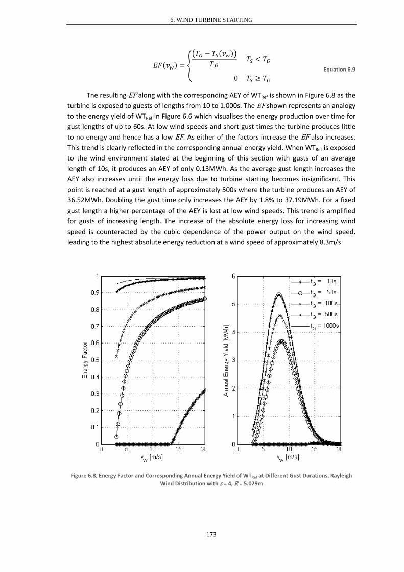
6. WIND TURBINE STARTING
𝐸𝐸𝐸𝐸(𝑣𝑣𝑤𝑤) = ��𝑇𝑇𝐺𝐺 − 𝑇𝑇𝑃𝑃(𝑣𝑣𝑤𝑤)�
𝑇𝑇𝐺𝐺 𝑇𝑇𝑃𝑃 < 𝑇𝑇𝐺𝐺
0 𝑇𝑇𝑃𝑃 ≥ 𝑇𝑇𝐺𝐺
Equation 6.9
The resulting EF along with the corresponding AEY of WTRef is shown in Figure 6.8 as the turbine is exposed to guests of lengths from 10 to 1.000s. The EF shown represents an analogy to the energy yield of WTRef in Figure 6.6 which visualises the energy production over time for gust lengths of up to 60s. At low wind speeds and short gust times the turbine produces little to no energy and hence has a low EF. As either of the factors increase the EF also increases. This trend is clearly reflected in the corresponding annual energy yield. When WTRef is exposed to the wind environment stated at the beginning of this section with gusts of an average length of 10s, it produces an AEY of only 0.13MWh. As the average gust length increases the AEY also increases until the energy loss due to turbine starting becomes insignificant. This point is reached at a gust length of approximately 500s where the turbine produces an AEY of 36.52MWh. Doubling the gust time only increases the AEY by 1.8% to 37.19MWh. For a fixed gust length a higher percentage of the AEY is lost at low wind speeds. This trend is amplified for gusts of increasing length. The increase of the absolute energy loss for increasing wind speed is counteracted by the cubic dependence of the power output on the wind speed, leading to the highest absolute energy reduction at a wind speed of approximately 8.3m/s.
Figure 6.8, Energy Factor and Corresponding Annual Energy Yield of WTRef at Different Gust Durations, Rayleigh Wind Distribution with s = 4, R = 5.029m
173

6. WIND TURBINE STARTING
Following the analysis of the source for the energy yield of the full scale WTRef over the period of 1 year, an analysis of the total AEY for WTRef, WTP, WTT and WTP-T at the 5.029m and 0.334m scale is presented in Figure 6.9.
Figure 6.9, Annual Energy Yield of WTRef, WTP, WTT and WTP-T as the Turbines are Exposed to Different Average Gust Lengths, Rayleigh Wind Distribution with s = 4
The investigation showed that blade pitch has a greater effect on the rotor’s AEY than blade thickness as it has been observed in section 5.2, 5.3 and 5.4 for cP. For long gust lengths of 1.000s the highest AEY is achieved by WTT with 39.71MWh for the full scale rotor and 0.15MWh for the small turbine for the given wind environment. As the average gust length decreases, the AEY for all rotors drops, however the small turbines are able to withstand gust reductions for longer than their larger counterpart before they experience a more rapid AEY drop which indicates significant Reynolds number effects. WTT sustains the highest AEY production until the average gust length decreases below 19.4s for the full scale rotors and 5.0s for the small scale rotors. Below these gust lengths WTP-T produces the highest AEY for both rotor scales. The continuously better performance of the thin blades is in contrast to the
174
6. WIND TURBINE STARTING
aerodynamic performance of the thicker bladed WTRef. WTRef outperforms WTT for nearly all λ below 4.9 as shown in Figure 5.13 but the reduced blade inertia of WTT and its higher cP at high λ give the thin bladed turbines their starting performance advantage. The higher energy yield during a single start of the thin bladed rotor, whether it is pitched or not, is also reflected by the shaded area in Figure 6.6 for the full scale rotors and in Figure 6.7 for the small scale rotors. More detailed underlying aerodynamic reasons for this pitch-thickness behaviour are described in detail in section 5.4. Their consequence on turbine starting has been investigated in section 6.2.2.
The analysis of the influence of the rotor blade geometry therefore indicates that thin bladed turbines are favourable for a high AEY, independently of the gustiness of the environment. However blade pitch may be used to maximise the AEY for particularly gusty environments. Especially for small turbines a larger effect of blade pitch on their energy yield has been observed. This is due to ultra-low Re effects which effect blades of different thicknesses to a different degree at different radii as described in section 5.3.3.
6.4 Summary
In this chapter a thorough analysis of the effect of the turbine geometry on its starting sequence has been presented for the reference NREL Phase VI turbine analysed in chapter 4 and the same 3 blade designs as those investigated in chapter 5, as they accelerated from rest to full operational speed. The analysis was conducted for a rotor radius of 5.029m and a wind speed of 6m/s and was based on the steady turbine performance evaluated in chapter 4 and 5. Following was a detailed study on the role of the starting sequences of all 4 turbine designs on the turbines energy yield as they are subjected to gusts of wind speeds ranging from 3 to 20m/s which last for 0 to 60s. The chapter was concluded with an annual energy analysis in order to address the stochastic nature of wind. The investigations were carried out for a rotor scale of 0.334 and 5.029m.
Turbine Starting Sequences
The observed trends for all of the analysed starting sequences followed those that have been documented in literature. The full scale NREL Phase VI turbine requires 46.6s and 7.42 revolutions to finish a complete starting sequence which can be divided into 3 distinct stages.
• Near uniform Re along blade at λ = 1.97: Before this λ the turbine experiences nearly no increase in its very low acceleration as most of the torque is produced at the blade root at a high α. The ultra-low λ - torque performance contributes the most towards the turbine starting time due to the very low torque production. The turbine
175

6. WIND TURBINE STARTING
experience insignificant performance reducing Re effects in this low λ operating range due to the heavy stall of the flow around the blade.
• α < 22° at the blade tip: This first occurs λ = 2.48. A higher acceleration is observed when α drops below this critical value which allows flow attachment to the suction surface. The acceleration rate continues to increase with increasing λ.
• Entire blade span experiences α < 22°: This occurs at λ = 4.25. At this stage the leading edge vortex is very small and the flow on the suction surface is at least partially attached. The continuous decrease in the torque production of the pressure surface however causes the net torque to decrease thereafter.
The effect of turbine pitch was found to dominate that of blade thickness. Significant alterations in the starting characteristics of the remaining turbine geometries were observed as follows:
• Pitching the reference turbine by 10° reduced its starting time by 79%. This reduction is mainly caused by a significantly higher starting torque due to a more favourable pressure to torque translation and by a drastically reduced λ of 1.6 at which the blade tip experiences α < 22°.
• Reducing the blade thickness reduced the staring time further for the un-pitched and pitched configurations. This is dominantly caused by a reduction of the blade’s inertia. A shift of the high torque producing α from 22° to 19° allows the thin blades to reach a relatively high cP.
Energy Output
The energy yield produced by a turbine depends on both, the rotor’s design cP at the current operating wind speed and its availability, the time during which the turbine produces power. The generator was assumed to impose no resistive torque on the turbine and only extract energy when the starting sequence is complete and the turbine rotates at its design cP.
• A turbine’s starting time can be estimated using its cT performance. When the turbine experiences insignificant Re effects during its entire starting sequence, the starting time scales with wind speed 𝑇𝑇𝑟𝑟 ∝ 𝑣𝑣𝑤𝑤−1 and turbine radius 𝑇𝑇𝑟𝑟 ∝ 𝑅𝑅. The relatively high Re dependence of small scale rotors causes them to experience a relative increase in their starting time and thus benefit more from a good rotor design.
• Pitching the reference turbine by 10° was observed to significantly improve and extend its low wind speed energy production when starting from rest during a gust. The higher energy yield is exclusively caused by a much shorter starting time, as the pitched rotor produces significantly less power than the un-pitched rotor.
• Reducing the blade thickness from 21 to 15% yields the highest design power coefficient but is characterised by a starting time that is between that of the reference rotor and the pitched rotor. The thin bladed rotor therefore produces the highest energy yield in flow environments with comparatively long gusts.
176

6. WIND TURBINE STARTING
• A pitched rotor with reduced thickness produces the highest energy yield during comparatively short gusts as it produces a similar power to the thick bladed rotor but at a reduced starting time.
Annual Energy Yield
The annual energy output of a turbine depends on the geometry of the particular turbine and the wind environment in which it is paced. A Rayleigh wind distribution with a shape parameter of 4 has been assumed along with a turbine availability of 70% during the period of one year which is composed of gusts of varying length.
• The annual energy performance of the full scale NREL Phase VI becomes independent of its starting performance as the gust length becomes larger than 1.000s. In this wind environment the turbine produces 37.19MWh. As the gust length decreases the annual energy output also decreases, hereby the highest percentage of the energy reduction occurs at low wind speeds.
• The annual energy output of all 4 rotors investigated reflects the previously established Reynolds number dependences as well as non-linear blade pitch and thickness interactions. For decreasing gust lengths these interactions lead to a delayed but more abrupt reduction of the energy yield of the small scale rotors than for the full scale turbines.
• The thin bladed turbine produces the highest annual energy output regardless of the gust length. A large blade pitch however becomes important for sustaining a high annual energy yield in gusty wind environments.
177

7. CONCLUSIONS AND RECOMMENDATIONS
7.1 Introduction
This thesis has investigated the role of turbine starting of small scale horizontal axis wind turbines on their energy yield using CFD. Small scale turbines have received much less research attention although they face a number of performance reducing issues which reduce the aerodynamic torque while simultaneously increasing the resistive generator torque, that large scale rotors do not experience. Resulting from insufficient scientific literature, the following key issues have been identified and subsequently investigated in this dissertation:
• A time accurate CFD method has been derived to model turbine starting. This model was also used to assess the assumptions of commonly used BEM theories. Through the use of CFD, a much higher level of detail of the flow was available for the analysis in this thesis.
• The detailed flow resolution was used to improve the understanding of turbine starting by analysing the underlying flow features which determine a turbine’s starting performance and conducting systematic studies on the effect of turbine geometry, namely blade pitch and blade thickness. Throughout this thesis the NREL Phase VI blade served as reference rotor. This analysis was conducted at different wind speeds and turbine radii.
• The knowledge gained has then be used to recommend favourable turbine geometries tailored to a specific turbine’s site, its radius and operating environment to maximise its annual energy yield.

7. CONCLUSIONS AND RECOMMENDATIONS
7.2 Modelling of Turbine Starting
In this thesis a computational fluid dynamics approach has been used to model turbine starting as it allowed the flow field around the rotor to be analysed which is not possible using BEM codes. Furthermore BEM inherent limitations such as assuming no radial cross flow and not accounting for 3D effects were also eliminated. A high fidelity, yet cost effective CFD methodology was developed to model a rotor as it accelerates from rest to full operational speed. Progressively more complex investigations on suitable CFD methodologies revealed that the k-ω SST turbulence model predicted the most accurate turbine performance over a range of rotational speeds with a good prediction consistency. The use of a hybrid mesh significantly reduced the computational time while still allowing critical areas to be resolved sufficiently.
A literature review on modelling turbine starting showed that very little research has been conducted on the validity of the frequently used steady state assumption when simulating a turbine start-up. Published research results furthermore indicate contradictory results. To address this shortcoming, a new method of simulating turbine starting has been developed by the author of this thesis. The CFD code Fluent has been provided with a script to simulate a fully transient turbine starting sequence using an inertia model. This highly computationally demanding method was then compared against quasi-steady starting sequences derived from constant rotational speed simulations using CFD and BEM. The simulations were conducted at 0.5 tip speed ratio intervals while keeping the wind speed constant. This is the first study addressing such a comparison between the different modelling methods. The investigation revealed that the quasi-steady CFD method produced an error of less than ±1.5% for the prediction of the design λ, the starting time and the maximum cP with respect to the transient method. The BEM method has been shown to be in good agreement with both CFD methods at low λ. At high λ the BEM method predicted a higher cT, leading to a higher cP. The predicted starting time however is nearly identical. It has been concluded that both modelling approaches may be used for modelling turbine starting during a constant wind. However when aiming to compare the starting performance of similar blades, a CFD computation is preferable as limitations in the derivation of BEM codes and difficulties in obtaining accurate aerodynamic input data at high angle of attack may obstruct correctly accounting for delicate flow features which affect the turbine’s starting performance. CFD furthermore provides flow details that are not resolved when using BEM codes, although its computational time is significantly longer than that of BEM.
When comparing the energy yield predicted during a gust using the quasi-steady CFD method to that predicted by the transient simulation, the error accumulates right after the generator is engaged but drops down exponentially to less than 6% when the turbine produces energy for more than 11s. The associated 12 fold increase in the computational time when using the fully transient method however did not justify its use. The accuracy and validity of the quasi-steady method for simulating turbine starting sequences has therefore been proven for the first time to the author’s knowledge.
179

7. CONCLUSIONS AND RECOMMENDATIONS
7.3 Improving the Understanding of Turbine Starting
As a turbine accelerates from rest to full operational speed it experiences a wide range of complex flow phenomena arising from a change of the local angle of attack and Reynolds number along the blade span as well as in time. At low rotational speeds the aerodynamics feature high angles of attack in combination with low Reynolds numbers. The revelations in this thesis are first presented in generic, non-wind-turbine specific form and are then brought into context for the isolated effects of varying blade pitch and blade thickness. Finally their interaction when modifying blade pitch and thickness simultaneously has been evaluated.
7.3.1 Generic Turbine Starting Conclusions
• The turbine starting time depends on aerodynamic blade torque ∝ ∫ 1𝑐𝑐𝑇𝑇𝑑𝑑𝜆𝜆 . The low λ
performance is most critical to turbine starting due to the low cT at low λ. • The cT production along a blade surface depends on the pressure distribution and its
translation into torque. The pressure distribution is affected by the flow features which in turn depend on the curvature of the local blade surface. The blade surface gradient also determines the pressure to torque translation.
• At ultra-low λ the blade root generates most of the torque due to a lower α and higher Re than the tip. The formation of large leading and trailing edge vortices behind the suction surface of approximately equal strength cause the cT along the blade surface to be predominantly influenced by the blade curvature rather than flow features. Both, the pressure and suction surface generate positive torque but that of the suction surface is increasing with increasing λ while that of the pressure surface decreases. The decrease is caused by the formation of larger areas producing negative torque for increasing λ. These areas arise from an increasingly more rapid pressure drop below zero from the leading edge for higher rotational speeds.
• As the blade rotational speed increases, the local Re along the blade becomes nearly uniform at λ = 1.97, for the NREL Phase VI rotor. This makes the radial cT primarily a function of α. The lower α at the blade tip thus shifts the region producing most of the torque from the root to the blade tip, causing an increase in the turbine acceleration as the lower α acts to push the trailing edge vortex towards the trailing edge and significantly reduce the thickness of the leading edge vortex.
• An even steeper increase in rotor acceleration is observed when α at the blade tip drops below a profile specific angle giving a high cL to cD ratio. This rapid increase in blade acceleration is terminated when the entire blade experiences α below that angle as the trailing edge vortex has completely vanished at this stage and the leading edge vortex has nearly completely disappeared.
• Following is a reduction in the net cT but the blade is allowed to accelerate further for as long as the increase in λ can compensate the combined reduction of cT of the pressure and suction surface, as this leads to a net cP increase.
180

7. CONCLUSIONS AND RECOMMENDATIONS
7.3.2 Conclusions of Geometry Influence on Turbine Starting
Relevant geometrical features that were observed to alter the turbine starting characteristics or maximum power production in this work are listed below. The summary includes relevant aspects from the entire thesis. Respective turbine starting times and maximum cP’s have been evaluated with respect to the full scale reference rotor. The rotors had a radius of 5.029m and operated at a wind speed of 6m/s.
Blade Pitch (WTP)
A blade pitching angle of 10° has been analysed. The investigated rotor with pitched blades generated a higher torque for any given λ up until its design λ due to two distinct mechanisms:
• Pitching a blade reduces its local geometric α by the amount the blade is pitched by, leading to more favourable flow features. The reduction of α affects the blade’s performance in multiple ways:
o The formation of smaller leading and trailing edge vortices due to blade pitch which disappear at a lower λ. The flow features formed around the pitched blade resemble those of the un-pitched blade operating at a higher λ. At low λ this difference is relatively small, but increases as λ of the pitched rotor increases.
o The reduction of α allows the blade tip to significantly contribute towards the blade’s total cT at a lower λ and thus produces a more uniform radial cT distribution throughout the entire operating range.
o The pitched blade reaches its high cT producing α of 22° at λ = 1.6 instead of at 2.5 as reference rotor and thereby initiates the rapid turbine acceleration phase at a lower λ.
• The resulting pressure distribution on a pitched blade is subjected to a more favourable pressure-to-torque translation which is caused by a change of the local blade surface curvature with respect to the rotational plane due to pitching. A negative pressure on the suction surface produces almost exclusively positive torque when the NREL Phase VI rotor is pitched by 10° but results in the generation of significant negative torque when the rotor is not pitched.
These aspects significantly shorten the starting time but also reduce the maximum cP as the suction surface cannot generate enough positive torque anymore due to a too low α. Pitching the full scale NREL Phase VI rotor operating at a 6m/s wind speed by 10° reduced the starting time by 79% and its maximum cP by 52%.
181

7. CONCLUSIONS AND RECOMMENDATIONS
Blade Thickness (WTT)
The effect of blade thickness has been evaluated by reducing the maximum thickness of the S809 aerofoil of the NREL Phase VI rotor of 0.21c to a maximum thickness of 0.15c. The following findings were revealed:
• The effect of modifying the blade thickness is of secondary order compared to blade pitching effects as it only moderately changes the local blade surface gradients but does not affect the local α. The characteristics of the torque producing radial sections are therefore similar to that of the reference NREL Phase VI rotor.
• While the suction surface suffers from a reduced blade thickness, the pressure surface profits from a thin blade. The flow only attaches to the suction surface at a higher λ due to the high adverse pressure gradient imposed by the smaller radius of the leading edge. Furthermore once it is attached, less energy can be extracted due to the flatter aerofoil centre. For the pressure surface the lower pressure drop implies that it will not generate negative torque as quickly.
• Reducing the blade thickness of the S809 profile from 21 to 15% causes α at which a significant increase in torque production is observed to drop from 21° to 19°. This in turn shifts λ during which rapid turbine acceleration is observed from 2.5 < λ < 4.3 for the reference blade to 2.9 < λ < 4.7 for the thin blade and thereby allows the thin bladed rotor to reach a higher cP.
These factors act to increase the cP by 7% and would incur a 10% longer starting time. Due to the lower turbine inertia of the thin bladed rotor however, the actual starting time is reduced by 22% with respect to the NREL Phase VI machine.
Combined Blade Pitch and Thickness (WTP-T)
• Modifying blade pitch and thickness affects the local blade surface curvature and geometric α. Of all the turbines investigated, the pitched, thin bladed turbine possesses the most favourable pressure-to-torque translation surface gradients.
• Blade pitch and thickness interact non-linearly producing a torque enhancement except for when the rotor operates at 1.5 < λ < 2.7. The underproduction of torque occurs over the λ range where pitching allows the flow around the thick blade to at least partially attach while the flow around the pitched thin blade still cannot attach due to a too high adverse pressure gradient caused by the high blade surface gradient at the leading edge.
• The profile dependent α at which a high cT is produced of 19° causes the blade to accelerate rapidly from λ = 1.8.
This results in a 53% lower cP of the pitched, thin bladed rotor than the NREL Phase VI turbine and a 66% reduction of starting time, of which 29% can be attributed to a reduced rotor inertia and the remaining 71% to improved aerodynamics.
182

7. CONCLUSIONS AND RECOMMENDATIONS
7.4 Increasing Annual Energy Yield
This thesis has been concluded with recommendations for preferred turbine designs while considering turbine site and rotor radius in order to maximise annual energy yield, which in turn depends on the rotor’s starting time and its cP production. To the author’s knowledge, this is the first investigation of its kind.
For a given turbine design, smaller rotors are able to harness wind energy at lower wind speeds and in more unsteady flow environments due to their shorter starting times than large turbines. Small rotors however show a comparatively high dependence of their energy yield on wind speed. Reynolds number effects cannot be ignored for the energy yield estimation of rotors with a radius of much less than 5m. Even at a 5m radius scale, turbines experience mild Reynolds number effects. Estimating the starting time of a small scale rotor using the
theoretical linear relationships of ∝ 𝑅𝑅 and ∝ 1𝑣𝑣𝑤𝑤
leads to a significant underestimation of the
starting time and hence overestimates the wind energy that can be harnessed. The Reynolds number effects have further been observed to be blade geometry dependent although at λ < 1.6 the very large flow separation eliminates Reynolds number effects. For both investigated turbine scales the pitched rotor is more prone to Reynolds number effects, irrespective of blade thickness.
A clear interdependence between turbine scale and the optimum combination of blade pitch and blade thickness has been shown, which demonstrates the capability of maximising the energy yield by designing a turbine tailored to the scale of the rotor. Turbine locations which require the rotor to frequently restart, such as in an urban environment, benefit from pitched blades. Reducing the blade thickness up to the structural limits of the rotor further increases the energy yield. Non-linear interactions between blade pitching and blade thickness effects significantly contribute towards a short rotor starting time and a favourable cP performance. Rotors with a very low radius particularly benefit from a reduced blade thickness when they are placed in a low wind speed environment due to ultra-low Reynolds number effects where viscous forces allow the flow to stay attached when flowing past a sharp leading edge. Avoiding flow separation leads to an improved torque performance of the suction surface.
The aerodynamic and structural findings of the thesis have been placed in context of the annual energy yield produced by the turbines previously analysed. The rotors were subjected to a Rayleigh wind distribution with a shape parameter of 4. The annual turbine availability has been assumed to be 70% which has been interrupted by gusts of different lengths. In this environment the full scale NREL Phase VI rotor produces an annual energy output of 37.19MWh when the gust lengths are longer than 1.000s. At shorter gust lengths the loss of the energy captured due to more frequent turbine starting becomes significant. When scaling the rotor down the gust length at which it experiences significant energy yield losses decreases. This enables small rotors to perform better than larger ones in a turbulent environment. It has therefore been concluded that although small scale turbines cannot reach the same cP as large scale rotors due to Reynolds number effects, they are more resistant
183

7. CONCLUSIONS AND RECOMMENDATIONS
energy yield reductions due to gusty environments. With respect to their starting performance they are therefore more suited for turbulent cites such as urban areas.
Varying blade thickness and pitch have revealed additional insights into the role of a rotor’s starting performance on its annual energy yield. Thin bladed turbines have been shown to consistently deliver a higher annual energy output than their thicker counterparts, regardless of the gustiness of the environment. This is mainly due to a better starting performance which is predominantly caused by the reduction of the blade inertia. The energy yield of the thin bladed turbines in gusty environments has furthermore been found to increase when pitching the blade. Pitching a small thin bladed turbine has been illustrated to have a larger effect on its energy yield than pitching a larger rotor due to the aforementioned Reynolds number dependent non-linear pitch thickness interactions. The thin bladed small scale rotor which has a thickness of 0.15c has been found to produce the highest energy yield in its 10° pitch configuration when the gust time is less than 5.0s. For longer gust times a lower pitch is recommended. The equivalent gust length for the full scale rotor is 19.4s.
7.5 Recommendations
Literature on turbine starting only started to emerge from the 90’s. Fundamental questions regarding the modelling of turbine starting and the role of turbine design were raised but have often not been thoroughly verified and validated. Instead, simplifying assumptions, such as the validity of a quasi-steady assumption for modelling turbine starting, have been made. This dissertation has successfully addressed some of those issues, but due to the complexity of the subject, there is still a range of topics to be investigated to further the understanding of start-up modelling and the effect of different turbine configurations.
7.5.1 Start-Up Modelling
Due to the research area of turbine starting being a relatively young one, a number of suggestions to improve the accuracy of turbine start-up models have been made in the experimental and computational field.
Experimental Methods
A relatively small number of studies experimentally investigating turbine starting have been published. All of those studies were conducted as field tests, not offering the controlled environment of wind tunnel experiments. This not only makes it difficult to avoid undesired
184

7. CONCLUSIONS AND RECOMMENDATIONS
flow fields, but also to isolate the effects of individual parameters of interest for turbine starting.
To address this issue, turbine start-up experiments of the NREL Phase VI rotor geometry scaled down to a radius of 0.334m were planned in the wind tunnel of the University of Sheffield. However due to problems with the measuring equipment, these experiments could not be conducted. It is therefore recommended that such experiments are conducted to create a reference database for the validation of computational methods. Unlike the turbines used in field tests, which have often only been equipped with a rotational speed sensor, additional measurements systems such as torque transducers can be installed during wind tunnel tests, delivering high quality validation data that as of today is not available in literature.
Computational Methods
The use of high fidelity CFD computations to model turbine starting in this dissertation enabled new insights into modelling approaches and starting analysis. While this is an important step towards designing more suited turbine blades for unsteady flow environments, this research field would benefit from extended computational method studies that were outside the scope or time constraint of this thesis.
Within the scope of this study different one and two equation turbulence models from the S-A, k-ε and k-ω turbulence model families have been investigated. Although some of them performed better than others, no model consistently delivered superior performance over the entire wind turbine operating range. A potential cause for this has been identified as the use of fully turbulent turbulence models. The use of more complex models with more transport equations or transitional models which also account for laminar flow is therefore recommended. This becomes more crucial when simulating wind turbines with a very small radius.
The quasi-steady assumption for modelling turbine starting has been validated for the first time on a rotor with 5.029m radius. This scale was chosen as detailed experimental measurements for the steady performance of the NREL Phase VI rotor have been available for validation purposes. As the turbine radius decreases however the rotor acceleration increases, making the occurrence of unsteady effects from flow transition or hysteresis more likely. It is therefore recommended to conduct studies on when unsteady effects become significant and their influence on the simulation of micro turbines.
The findings of such computational CFD studies could then be used to improve BEM methods to ensure a fast, yet accurate prediction of the starting performance of small scale turbines and their corresponding energy yield. When investigating highly complex flow environments or a large number of flow conditions along with different turbine geometries, as it should be done when designing a new rotor, it is not economical to use CFD anymore. BEM methods on the contrary provide a good alternative.
185

7. CONCLUSIONS AND RECOMMENDATIONS
7.5.2 Turbine Configurations
The systematic studies presented in this thesis investigated the effect of changing turbine scale, blade pitch and blade thickness as well as their combined effect for the first time. Each parameter has been varied by a significant amount in order to clearly observe their basic effect. While this provides a good base for investigating each parameter, the analysis would significantly benefit from a refined parameter study. This would essentially allow the generation of a detailed performance matrix indicating the amount of interaction of the investigated parameters in terms of resulting flow features, turbine starting time and maximum cP. The study conducted on the combined effect of blade thickness and pitch suggests that there is a significant amount of non-linear parameter interaction. Furthermore, in this thesis only linear trends when modifying a single parameter have be shown as not enough turbine geometries have been generated to visualise more complex trends. This however is likely to obscure the location of global performance maxima and minima. Identifying the optimum blade pitch and thickness for turbines of different radii would be a practical application of such an analysis.
The present analysis moreover only investigated a small selection of turbine parameters. There is a high potential for the energy yield produced by a rotor to be further increased when considering more blade geometry parameters:
• The aerodynamic profile can be varied and mixed aerofoil blades can be studied. Studies investigating the effect of using thick profiles at the blade root for structural purposes and thin profiles at the blade tip may be conducted.
• The twist and chord distributions along the blade radius can be varied by applying functions whose coefficients may be modified. This could be used for optimisation studies.
• The use of a variable blade pitch mechanism has been experimentally shown to significantly reduce the rotor’s start-up time. As technology advances, this may become a viable mechanism for small scale rotors and is therefore of interest. It is also more likely to induce unsteady flow phenomenon and thereby provides the ground for interesting computational studies.
Once solid modelling techniques have been developed and favourable turbine designs identified, the simulation complexity can be increased, resulting in a closer match to real-life wind environments. By doing so, the preferred turbine design producing the highest energy yield is likely to change, indicating an iterative nature of the process of finding the most suited turbine design for a specific wind environment. Especially for low wind speed environments, a high potential for the increase of the energy yield has been demonstrated. It is suggested to investigate the following parameters:
• Wind environment: Conducting simulations with high turbulence intensities and/or changing wind velocity resemble the flow environment of small scale rotors placed in an urban environment much better. Furthermore detailed studies on changing wind directions inducing yawed turbine flow are recommended. When increasing the rate
186

7. CONCLUSIONS AND RECOMMENDATIONS
of change of the suggested parameters hysteresis effects might be induced, emphasising on the necessity of using a high fidelity computational model.
• Complete Turbine: In order to gain realistic energy yield predictions from computational models, it is essential to consider the whole system. This includes modelling a complete small scale rotor with its tail fin and the rotors response to changes in the flow environment.
• Resistive torque: The performance of turbines with decreasing radius has been shown to be strongly influenced by the resistive torque imposed on the turbine from its generator. While an investigation of the effect of a generator model has been outside the scope of this dissertation, it is worth conducting such a study as this allows to not only draw conclusions about preferred turbine designs but also suitable generator configurations as well as any interdependence between the aforementioned aspects.
187

8. REFERENCES
[1] E. Hau, Windkraftanlagen - Grundlagen, Technik, Einsatz, Wirtschaftlichkeit vol. 4: Springer, 2008.
[2] S. Eriksson, et al., "Evaluation of different turbine concepts for wind power," Renewable and Sustainable Energy Reviews, vol. 12, pp. 1419-1434, 2008.
[3] P. W. Carlin, et al., "The History and State of the Art of Variable-Speed Wind Turbine Technology," 2001.
[4] The Wincharger Corporation. Available: http://www.windcharger.org/Wind_Charger/ Wincharger.html
[5] (2011). Jacobs Wind Electric co. inc. Available: http://www.jacobswind.net/history/ original-company
[6] "Carbon Footprint of Electricity Generation," 2006.
[7] RenewableUK, "Small Wind Systems UK Market Report," 2011.
[8] P. D. Clausen and D. H. Wood, "Recent advances in small wind turbine technology," Wind Engineering, vol. 24, pp. 189-201, 2000.
[9] (2012, 16.07.2012). Sintra 2001. Available: http://www.sintra2001.pt/images/ produtos/ energias/bergey/bergey5.jpg
[10] (2012, 16.07.2012). Blade Wind Tech. Available: http://www.blade-wind-tech.nl/ products/horizontal-axis/eol-wt/eol-100k
[11] A. W. E. Association, "A 20-year industry plan for small wind turbine technology," 2002.

8. REFERENCES
[12] IEC, "IEC 61400-2; Wind turbines - Part 2: Design requirements for small wind turbines," 2006.
[13] M. Aner, et al., Recent Advances in Converters and Control Systems for Grid-Connected Small Wind Turbines, 2012.
[14] P. D. Clausen and D. H. Wood, "Research and development issues for small wind turbines," Renewable Energy, vol. 16, pp. 922-927, 1999.
[15] S. O. Ani, "Low Cost Small Wind Turbine Generators for Developing Countries," Doctor of Philosophy, Technische Universiteit Delft, 2013.
[16] (2014, 02.08.). allsmallwindturbines. Available: http://www.allsmallwindturbines.com/ ?page=1&sort=turbine_d
[17] P. R. Ebert and D. H. Wood, "Observations of the starting behaviour of a small horizontalaxis wind turbine," Renewable Energy, vol. 12, pp. 245-257, 1997.
[18] F. Wang, et al., "The methodology for aerodynamic study on a small domestic wind turbine with scoop," Journal of Wind Engineering and Industrial Aerodynamics, vol. 96, pp. 1-24, 2008.
[19] S. Frandsen, et al., "Redefinition power curve for more accurate performance assessment of wind farms," Wind Energy, vol. 3, pp. 81-111, 2000.
[20] P. D. Clausen, et al., "The shape and performance of hand-carved small wind turbine blades," Wind Engineering, vol. 33, pp. 299-304, 2009.
[21] J. J. G. Michael S. Selig, Andy P. Broeren, Philippe Giguere, "Experiments on Airfoils at Low Reynolds Numbers," in 34th Aerospace Science Meeting & Exhibit, Reno, 1996.
[22] J. Breshears and C. Briscoe, "The informed application of building-integrated wind power," 2009.
[23] T. J. Mueller, et al., "The influence of free-stream disturbances on low Reynolds number airfoil experiments," Experiments in Fluids, vol. 1, pp. 3-14, 1983.
[24] D. H. Wood, "A blade element estimation of the cut-in wind speed of a small turbine," Wind Engineering, vol. 25, pp. 249-255, 2001.
[25] D. Wood, Small Wind Turbines - Analysis, Design, and Application, 2011.
[26] M. Hampsey and D. H. Wood, "Designing small wind turbine blades for optimal starting and power extraction," Wind Engineering, vol. 23, pp. 31-40, 1999.
[27] M. E. Bechly, Clausen, P. D., Ebert, P. R., Pemberton, A. and Wood, D. H., "Field testing of a prototype 5 kW wind turbine," in Proceedings of the 18th British Wind Energy Association Conference, Exeter, 1996, pp. 103-110.
[28] J. W. Sons, "The NREL Full-Scale Wind Tunnel Experiment," Wind Energy, vol. 5, pp. 77 - 84, 2002.
[29] H. Snel, "Review of Aerodynamics for Wind Turbines," Wind Energy, vol. 6, pp. 203 - 211, 2003.
189

8. REFERENCES
[30] A. K. Wright, "Aspects of the Aerodynamics and Operation of a Small Horizontal Axis Wind Turbine," Doctor of Philosophy, Department of Mechanical Engineering, The University of Newcastle, Newcastle, 2005.
[31] S. Worasinchai, "Small Wind Turbine Starting Behaviour," Doctor of Philosophy, University of Durham, Durham, 2012.
[32] D. H. Wood, "Dual purpose design of small wind turbine blades," Wind Engineering, vol. 28, pp. 511-528, 2004.
[33] M. J. Clifton-Smith and D. H. Wood, "Further dual purpose evolutionary optimization of small wind turbine blades," Journal of Physics: Conference Series, vol. 75, 2007.
[34] Euros, "Blade family EU 51 / 55 / 59," ed, 2009.
[35] M. M. Hand, et al., "Unsteady Aerodynamics Experiment Phase VI: Wind Tunnel Test Configurations and Available Data Campaigns," 2001.
[36] Z. Yang, et al., "An experimental investigation on aerodynamic hysteresis of a low-Reynolds number airfoil," 2008.
[37] L. J. Pohlen and T. J. Mueller, "Boundary Layer Characteristics of the Miley Airfoil at Low Reynolds Numbers," 1983.
[38] T. J. Mueller, "The Influence of Laminar Separation and Transition on Low Reynolds Number Airfoil Hysteresis," Journal of Aircraft, vol. 22, pp. 763-770, 1985.
[39] C. Rohrbach, et al., "Experimental And Analytical Research On The Aerodynamics Of Wind Driven Turbines," 1977.
[40] C. E. Carcangiu, et al., "CFD-RANS Analysis of the Rotational Effects on the Boundary Layer of Wind Turbine Blades," Journal of Physics: Conference Series, vol. 75, 2007.
[41] D. Hu, et al., "A study on stall-delay for horizontal axis wind turbine," Renewable Energy, vol. 31, pp. 821-836, 2006.
[42] P. K. Chaviaropoulos and M. O. L. Hansen, "Investigating three-dimensional and rotational effects on wind turbine blades by means of a quasi-3D Navier-Stokes solver," Journal of Fluids Engineering, Transactions of the ASME, vol. 122, pp. 330-336, 2000.
[43] M. Alam, et al., "The ultra-low Reynolds number airfoil wake," Experiments in Fluids, vol. 48, pp. 81-103, 2010.
[44] Timmer and W. A. Timmer, "Two-dimensional low-Reynolds number wind tunnel results for airfoil NACA 0018," Wind Engineering, vol. 32, pp. 525-537, 2008.
[45] P. Devinant, et al., "Experimental study of wind-turbine airfoil aerodynamics in high turbulence," Journal of Wind Engineering and Industrial Aerodynamics, vol. 90, pp. 689-707, 2002.
[46] M. S. Selig, "Low Reynolds Number Airfoil Design - Lecture Notes," University of Illinois at Urbana-Champaign2003.
[47] B. Berges, "Development of Small Wind Turbines," M.Sc Thesis, Department of Mechanical Engineering, Technical University of Denmark, 2007.
190

8. REFERENCES
[48] A. K. Wright and D. H. Wood, "The starting and low wind speed behaviour of a small horizontal axis wind turbine," Journal of Wind Engineering and Industrial Aerodynamics, vol. 92, pp. 1265-1279, 2004.
[49] J. Bumby, et al., "A Permanent Magnet Generator for Small Scale Wind Turbines," in Proceedings of the 17th International Conference on Electrical Machines, Chania, Crete, Greece, 2006.
[50] C. Mayer, et al., "The starting behaviour of a small horizontal-axis wind turbine," Renewable Energy, vol. 22, pp. 411-417, 2001.
[51] O. Ozgener and L. Ozgener, "Exergy and reliability analysis of wind turbine systems: A case study," Renewable and Sustainable Energy Reviews, vol. 11, pp. 1811-1826, 2007.
[52] R. A. Kishore, "Small-scale Wind Energy Portable Turbine (SWEPT)," Master of Science, Mechanical Engineering, State University, 2013.
[53] IEC, "Wind turbines - Part 12.1: Power performance measurements of electricity producing wind turbines," 2005.
[54] T. Maeda, et al., "Surface Pressure Distribution on a Blade of a 10 m Diameter HAWT (Field Measurements versus Wind Tunnel Measurements)," Journal of Solar Energy Engineering, vol. 127, pp. 185-191, 2005.
[55] S. J. Miley, "Catalog of low-Reynolds-number airfoil data for wind-turbine applications," 1982.
[56] I. Gursul, et al., "Effects of time scales on lift of airfoils in an unsteady stream," AIAA journal, vol. 32, pp. 797-801, 1994.
[57] J. H. Strickland and G. M. Graham, "Force Coefficients For A NACA-0015 Airfoil Undergoing Pitching Rate Motions," AIAA journal, vol. 25, pp. 622-624, 1987.
[58] F. Rasmussen, et al., "Dynamic stall and aerodynamic damping," Journal of Solar Energy Engineering, Transactions of the ASME, vol. 121, pp. 150-155, 1999.
[59] J. N. Sørensen, "Aerodynamic Aspects of Wind Energy Conversion," vol. 43, ed, 2011, pp. 427-448.
[60] H. M. Sørensen NN, "Rotor performance predictions using a Navier-Stokes method," presented at the 36th AIAA Aerospace Science Meeting 25, Reno, 1998.
[61] R. Mahu and F. Popescu, "NREL Phase VI Rotor Modeling and Simulation Using Ansys Fluent 12.1," 2010.
[62] J. O. Mo and Y. H. Lee, "CFD Investigation on the aerodynamic characteristics of a small-sized wind turbine of NREL PHASE VI operating with a stall-regulated method," Journal of Mechanical Science and Technology, vol. 26, pp. 81-92, 2012.
[63] N. Sezer-Uzol and L. N. Long, "3-D Time-Accurate CFD Simulations of Wind Turbine Rotor Flow Fields," presented at the Collection of Technical Papers - 44th AIAA Aerospace Science Meeting 7, 2006.
[64] E. P. N. Duque, et al., "Navier-Stokes and comprehensive analysis performance predictions of the NREL phase VI experiment," Journal of Solar Energy Engineering, Transactions of the ASME, vol. 125, pp. 457-467, 2003.
191

8. REFERENCES
[65] W. L. Oberkampf, et al., "Guide for the Verification and Validation of Computational Fluid Dynamics Simulations," AIAA, vol. AIAA-G-077-1998, p. 19, 1998.
[66] J. A. Ekaterinaris and F. R. Menter, "Computation of oscillating airfoil flows with one- and two-equation turbulence models," AIAA journal, vol. 32, pp. 2359-2365, 1994.
[67] Y. M. Park, et al., "Numerical simulation of wind turbine scale effects by using CFD," in 45th AIAA Aerospace Sciences Meeting and Exhibit, Reno, Nevada, 2007, pp. 2547-2556.
[68] S. Benjanirat, et al., "Evaluation of turbulence models for the prediction of wind turbine aerodynamics," 2003, pp. 73-83.
[69] C. Tongchitpakdee, et al., "Numerical Simulation of the Aerodynamics of Horizontal Axis Wind Turbines under Yawed Flow Conditions," Journal of Solar Energy Engineering, vol. 127, pp. 464-474, 2005.
[70] J. Y. You, et al., "Effect of turbulence models on predicting HAWT rotor blade performances," Journal of Mechanical Science and Technology, vol. 27, pp. 3703-3711, 2013.
[71] L. Davidson, An Introduction to Turbulence Models. Göteborg, Sweden: Chalmers University of Technology, Department of Thermo and Fluid Dynamics, 2009.
[72] C. L. Rumsey and P. R. Spalart, "Turbulence Model Behavior in Low Reynolds Number Regions of Aerodynamic Flowfields," presented at the 38th AIAA Fluid Dynamics Conference and Exhibit, Seattle, WA, 2008.
[73] L. Eça and M. Hoekstra, "Near-wall profiles of mean flow and turbulence quantities predicted by eddy-viscosity turbulence models," International Journal for Numerical Methods in Fluids, vol. 63, pp. 953-988, 2009.
[74] Fluent 14.0 Theory Guide.
[75] V. Gleize, et al., "Numerical and Physical Analysis of the Turbulent Viscous Flow Around a NACA0015 Profile at Stall," presented at the European Congress on Computational Methods in Applied Sciences and Engineering, 2004.
[76] K. Ameur, et al., "2D and 3D numerical simulation of the wind-rotor/nacelle interaction in an atmospheric boundary layer," Journal of Wind Engineering and Industrial Aerodynamics, vol. 99, pp. 833-844, 2011.
[77] A. M. AbdelSalam and V. Ramalingam, "Wake prediction of horizontal-axis wind turbine using full-rotor modeling," Journal of Wind Engineering and Industrial Aerodynamics, vol. 124, pp. 7-19, 2014.
[78] Fluent 12.0 Theory Guide.
[79] B.-S. Kim, et al., "3-D Numerical Predictions of Horizontal Axis Wind Turbine Power Characteristics of the Scaled Delf University T40/50 Model," presented at the The Fifth JSME-KSME Fluids Engineering Conference, Nagoya, Japan, 2002.
[80] N. N. Sørensen, et al., "CFD Computations of Wind Turbine Blade Loads During Standstill Operation," Risø National Laboratory, Roskilde, Denmark2004.
192

8. REFERENCES
[81] F. R. Menter, "Two-equation eddy-viscosity turbulence models for engineering applications," AIAA journal, vol. 32, pp. 1598-1605, 1994.
[82] N. N. Sørensen, et al., "Navier–Stokes predictions of the NREL phase VI rotor in the NASA Ames 80 ft × 120 ft wind tunnel," Wind Energy, vol. 5, pp. 151-169, 2002.
[83] F. Massouh and I. Dobrev, "Exploration and Numerical Simulation of Wind Turbine Wake," ISJAEE, vol. 62, pp. 163 - 168, 2008.
[84] D. K. Walters and D. Cokljat, "A three-equation eddy-viscosity model for reynolds-averaged navier-stokes simulations of transitional flow," Journal of Fluids Engineering, Transactions of the ASME, vol. 130, pp. 1214011-12140114, 2008.
[85] J. Windte, et al., "Validation of the RANS-simulation of laminar separation bubbles on airfoils," Aerospace Science and Technology, vol. 10, pp. 484-494, 2006.
[86] M. Costes, et al., "Grid Sensitivity Study for the Turbulent Viscous Flow Around a NACA0015 Airfoil at Stall," presented at the 31st ERF, Florence, 2005.
[87] S. Gómez-Iradi, et al., "Development and validation of a cfd technique for the aerodynamic analysis of HAWT," Journal of Solar Energy Engineering, Transactions of the ASME, vol. 131, pp. 0310091-03100913, 2009.
[88] S. Yang, et al., "Subsonic Flow over Unstalled Pitching Airfoil Computed by Euler Method," presented at the 36th AIAA Fluid Dynamics Conference and Exhibit, San Francisco, California, 2006.
[89] Fluent 12.0 User's Guide.
[90] N. Fujisawa, et al., "Measurements of wall-shear-stress distribution on an NACA0018 airfoil by liquid-crystal coating and near-wall particle image velocimetry (PIV)," Measurement Science and Technology, vol. 20, p. 065403, 2009.
[91] C. Sicot, et al., "Unsteady characteristics of the static stall of an airfoil subjected to freestream turbulence level up to 16%," Experiments in Fluids, vol. 41, pp. 641-648, 2006.
[92] A. L. Moigne, "A discrete Navier-Stokes adjoint method for aerodynamic optimisation of Blended Wing-Body configurations," Doctor of Philosophy, College of Aeronautics, Cranfield University, 2002.
[93] J. Laursen, et al., "3D CFD Quantification of the Performance of a Multi-Megawatt Wind Turbine," Journal of Physics: Conference Series, vol. 75, 2007.
[94] R. Yang and R.-n. Li, "Research of the Rotational Effects on the Aerodynamics Characteristics of Horizontal Axis Wind Turbine," IEEE, 2009.
[95] R. Mahu, et al., "3D CFD modeling and simulation of NREL phase VI rotor," 2011, pp. 1520-1523.
[96] T. Cho, et al., "Acoustic measurement for 12% scaled model of NREL Phase VI wind turbine by using beamforming," Current Applied Physics, vol. 10, pp. S320-S325, 2010.
[97] Eureka. Available: http://www.eureka.im/218.html
193

8. REFERENCES
[98] H. Schlichting and E. A. Truckenbrodt, Aerodynamik des Flugzeuges, 2. Auflage ed. vol. Erster Band: Grundlagen aus der Strömungsmechanik Aerodynamik des Tragflüglers (Teil I): Springer Verlag, 1967.
[99] I. H. Abbott and A. E. v. Doenhoff, Theory of Wing Sections: New York : Dover, 1959.
[100] B. Summerville, "Small Wind Turbine Performance in Western North Carolina," 2005.
194

9. APPENDIX
9.1 HAWT Meshing
Three different software were involved in generating a high quality mesh:
• Matlab: assembly of the blade geometry from profile, chord and twist data which was written into a Gridgen native ‘.net’ format
• Gridgen: import of .net file, generation of blade surface mesh, BL and far-field blocks, Blocks 1, 3 and 4 in Figure 3.12
• TGrid: generation of unstructured mesh, Block 2 in Figure 3.12
9.1.1 Matlab
The X and Y coordinates of the aerodynamic profiles of interest were modified to ensure a smooth blade surface and to round the trailing edge of the aerofoil from 0.99c.
A fully automated, user friendly Matlab script was written to generate the coordinates for the suction and pressure surfaces of the blade which were then exported in Gridgen’s ‘.net’ format. The script only required the name of the profile, its radial location, its chord length and its twist as well as the corresponding chord and twist axis as input. The structure of the ‘.net’ file is shown in Figure 9.1.

9. APPENDIX
Figure 9.1, Structure of Gridgen’s .net File
9.1.2 Gridgen
The structured BL was generated by inflating the fully structured surface mesh of the blade. The surface mesh was clustered around the leading and trailing edge of the blade as well as towards the tip to reach faster mesh independence as those regions are characterised by high flow gradients. For the extrusion to work it is vital to adjust the volume smoothing factor in Gridgen which controls how strictly the node clustering of the surface mesh is preserved as the extrusion marches outwards. If the default value is not drastically reduced the extrusion will not work due to the sharp corners of the blade. Table 9.1 shows the volume smoothing factor used for the meshes in this thesis in relation to the current extrusion step. The splay factor also had to be set to 0.
Line1: Number of Blade Surfaces N=2
Line 2: i, j, k Number of Grid Points in Each Dimension of Blade Surfaces
k=1 for a surface iN1 jN1 kN1
iN2 jN2 kN2 .net File
x, y, z & i, j, k Systems
i1 j1
x1 y1 z1 i2 j1
x2 y2 z2 i3 j1
x3 y3 z3 i4 j1
x4 y4 z4
i1 j2
x5 y5 z5 i2 j2
x6 y6 z6 i3 j2
x7 y7 z7 i4 j2
x8 y8 z8
i1 j3
x9 y9 z9 i2 j3
x10 y10 z10 i3 j3
x11 y11 z11 i4 j3
x12 y12 z12
Remaining Lines: x, y, z Coordinates of Grid Points
x1 x2 x3 … y1 y y3 … for entity 1 z1 z2 z3 … x1 x2 x3 … y1 y y3 … for entity 2 z1 z2 z3 …
196

9. APPENDIX
Extrusion step Volume smoothing factor
0 – 5 5e-5 6 – 10 1e-4
11 – 15 1e-3 16 – 20 1e-2 21 – 25 0.1 26 – 30 0.3
31 – BL edge 1
Table 9.1, Suitable Volume Smoothing Factors for BL Extrusion
9.2 Useful Fluent TUI Commands
Some of the commands used for the simulations in this thesis are only available through the Text User Interface (TUI).
• monitor residuals in every cell, they can then be analysed in contour plots o /solve/set/expert y n n
• Create multiple conformal periodic zones o /mesh/modify-zones/make-periodic [ID_1] [ID_2]
• Converting from MRF to sliding mesh simulation o /mesh/modify-zones/mrf-to-sliding-mesh [block_ID]
• Use data file for case files with different mesh densities o /file/interpolate/write-data path/file_name.ip o /file/interpolate/read-data path/file_name.ip
9.3 Turbulence Model Analysis & Mesh Analysis
The colour coding of all contour plots in section 9.3.1 to 9.3.6 as well as the X and Y axis labels are shown in Figure 9.2. For more details on the derivation of the contour plots in this section refer to section 3.2.2.
197
9. APPENDIX
Figure 9.2, Contour Plot Colour Coding and X and Y Labels
198

9. APPENDIX
9.3.1 Solver Study: Standard k-ɛ Model, EWT
Figure 9.3, Solver Performance Comparison using Standard k-ε Model with EWT, Data Compared with Devinant et al. [45]
199

9. APPENDIX
9.3.2 Solver Study: k-ɛ RNG Model, EWT
Figure 9.4, Solver Performance Comparison using k-ε RNG Model with EWT, Data Compared with Devinant et al. [45]
200

9. APPENDIX
9.3.3 S-A Model
Figure 9.5, S-A Model Analysis with Different Wall Treatments using Coupled Solver, Data Compared with Devinant et al. [45]
201

9. APPENDIX
9.3.4 k-ɛ Model, SWF
Figure 9.6, k-ε Model Analysis using SWF using Coupled Solver, Data Compared with Devinant et al. [45]
202

9. APPENDIX
9.3.5 k-ɛ Model, EWT
Figure 9.7, k-ε Model Analysis using EWT using Coupled Solver, Data Compared with Devinant et al. [45]
203

9. APPENDIX
9.3.6 k-ω Model
Figure 9.8, k-ω Model Analysis using SIMPLE Solver, Data Compared with Devinant et al. [45]
204

9. APPENDIX
9.4 Start-Up UDF
/* Description of UDF:
RPM calculation & pressure forces & moments
- update rpm based using inertia model
- positive turbine rotation is around -Y axis
- UDF has to hooked to all blade surfaces & rotating volume
First time set-up
1) open Fluent with default directory where UDF case & data files are saved
2) read converged case & data files
3) update first section of UDF according to blade surface ID's & block ID's etc in Fluent
4) ONLY for first time UDF use, change rotational speed in "omega_MP.txt" to 0
5) specify UDM's
-> Define -> User-Defined -> Memory... -> User Defined Node Memory -> 4
node-udm-0 = pressure torque
node-udm-1 = rate of change of pressure torque
node-udm-2 = viscous torque
node-udm-3 = rate of change of viscous torque
-> Define -> User-Defined -> Memory... -> User Defined Memory -> 5
udm-0 = x acceleration
udm-1 = y acceleration
udm-2 = z acceleration
udm-3 = static pressure
udm-4 = rate of change of static pressure
6) create surfaces over which contours are monitored
-> Surface -> Iso-Surface -> Surface of Constant "Mesh" "Radial Coordinate" -> Iso-Values ... -> New
Surface Name
... [no Surface or Zones selected]
-> Surface -> Iso-Surface -> Surface of Constant "Mesh" "Y Coordinate" -> Iso-Values ... -> New
Surface Name ... [no Surface or Zones selected]
205

9. APPENDIX
7) define scheme variables to export case&data files and Tecplot contour plots
-> Type in TUI menu: (rp-var-define 'wrt_case 0 'integer #f)
-> Type in TUI menu: (rp-var-define 'wrt_contour 0 'integer #f)
-> to check type: (%rpgetvar 'wrt_case)
8) define execute commands
-> Calculation Activities -> Execute Commands -> "case&data" -> Every 1 Time Step, Command:
(if (= (%rpgetvar 'wrt_case) 1) (ti-menu-load-string (format #f "fi wcd startup_%t.cas.gz")))
-> Calculation Activities -> Execute Commands -> "contour blade" -> Every 1 Time Step, Command:
(if (= (%rpgetvar 'wrt_contour) 1) (ti-menu-load-string (format #f "file export tecplot contour_blade_%t
pressure_surf-18 suction_surf-17 tip-16 () pressure node-udm-0 node-udm-1 node-udm-2 node-udm-3 ()")))
-> Calculation Activities -> Execute Commands -> "contour far-field" -> Every 1 Time Step, Command:
(if (= (%rpgetvar 'wrt_contour) 1) (ti-menu-load-string (format #f "file export tecplot contour_farfiled_%t
r_02 r_03 r_04 r_05 r_06 r_07 r_08 r_09 r_10 r_11 y_02 y_05 y_10 () pressure udm-0 udm-1 udm-2 udm-3
vorticity-mag relative-x-velocity relative-y-velocity relative-z-velocity ()")))
9) compile & load UDF
10) define Custom Field Functions (CFF) in Fluent
11) hooke EXECUTE_AT_ENDE & DEFINE_ZONE_MOTION DFD
12) write case & data
13) run simulation
Subsequent reading of case & data files
- no action required if it's read in the same PC again
- recompile UDF
Outputs
- case & data file saved whenever TSR condition is met
- 'Calculation Activities -> Execute Commands' has to be specified
- "Global_Torque.txt" exported every X time steps
- radius is discretised and torque values over each segment are summed
- ever line contains ['flow time' torque(r1/R) torque(r2/R) ... torque(rn/R)]
- all comands contained in UDF
- "Local_Torque_t_N" exported in Tecplot '.dat' format every X time steps
- surfaces: suction, pressure and tip (generated in meshing software)
- variables: total moment, dTorque/dt
- correct amount of User Defined Memory has to be allocated via GUI or journal
206

9. APPENDIX
- "Flow_Field_t_N" exported in Tecplot '.dat' format every X time steps
- surfaces: circular slices cutting blade & planes parallel to rotational plane (generated as ISO-surfaces in
Fluent)
- variables: vx, vy, vz, vmag, ps & derivatives of all
- correct amount of UDM has t obe allocated via GUI or journal
- Screen outputs:
- torque contibution of each blade surface & total torque every time step
- rotational speed that is applied to each time step
- various warnings if UDF is setup improperly
*/
#include "udf.h"
#include "math.h"
#include "mem.h"
#include "stdio.h"
static float omega1 = 0;
DEFINE_ZONE_MOTION (Update_Omega, omega, axis, origin, velocity, time, dtime)
{
/* DEFINE_ZONE_MOTION is called at the start of every timestep BEFORE the first iteration */
/* dtime - time step size */
/* time - physical flow time */
FILE *file_2 = fopen ("omega_MP.txt","r"); /* read rotational speed from file which is written by
EXECUTE_AT_ENDE for new time step */
if (file_2 == NULL)
{Message0("\nWARNING: File containing rotational speed does not exist!");}
else
{
while (!feof(file_2))
{fscanf (file_2, "%f", &omega1);}
fclose (file_2);
207

9. APPENDIX
}
*omega = omega1;
N3V_S(velocity,=,0.0);
N3V_S(origin,=,0.0);
N3V_D(axis,=,0.0,-1.0,0.0);
Message0("\n\nOmega = %f rad/s\n\n",*omega);
return;
}
DEFINE_EXECUTE_AT_END (Torque_transient_startup)
{
/* USER INPUT for moment calculation show me where the calculation is happening */
int no = 3; /* number surfaces on blade */
int thread_id [3] = {16,17,18}; /* vector containing all blade surface ID's */
int n_blks = 2;
int blk_id [2] = {2,14};
real inertia = 949;
real n_blades = 2; /* number of turbine blades */
#define n_print_1 50 /* time steps after which contours file are written*/
#define n_print_2 1 /* text output file */
/* write case & data */
real R = 5.029; /* turbine radius */
real vw = 6; /* wind speed at which turbine operates */
static real wrt [22] = {0.75,1,1.25,1.5,1.75,2,2.25,2.5,2.75,3,3.25,3.5,3.75,4,4.25,4.5,4.75,5,5.25,5.5,5.75,6};
/* TSR's at which case & data is written */
float r_min = 0.5; /* smallest radial coordinate of blade */
float r_max = 5.036; /* largest radial coordinate of blade */
208

9. APPENDIX
/***********************************************************************************/
/********************* START OF FUNCTION ******************************************/
/***********************************************************************************/
real dt = CURRENT_TIMESTEP;
real time = CURRENT_TIME;
/* Force and Moments Declarations */
real Force[ND_3], Force_viscous[ND_3], Force_pressure[ND_3],
Force_viscous_tot[ND_3], Force_pressure_tot[ND_3], Force_tot[ND_3], A[ND_3];
real Moment[ND_3], Moment_viscous[ND_3], Moment_pressure[ND_3],
Moment_tot[ND_3], Moment_viscous_tot[ND_3], Moment_pressure_tot[ND_3];
float F_vis[3][no], F_p[3][3],F_tot[3][3]; /* [3 for x,y&z values][3 for no of blade surfaces] */
float M_vis[3][no], M_p[3][3], M_tot[3][3];
/* Geometry Variable Declarations */
real r[ND_3]; /* radial coordinate*/
real origin [3] = {0,0,0}; /* centre of rotation*/
real xc[ND_3]; /* coordinates of face centroid */
N3V_S(xc,=,0.0); /* cell centroid coordinate */
N3V_S(r,=,0.0);
N3V_S(A,=,0.0); /* face Area */
/* Fluent pointers */
face_t f;
cell_t c;
Thread *ct;
Node *node;
Domain *domain = Get_Domain(1); /* 1 is for single phase flow */
int thread_n_id; int blk_n_id;
int i, j, n; /* for all for & if loops */
for(i=0; i<3; i++) /*x,y,z coordinates of origin transferred to all nodes */
{host_to_node_real_1(origin[i]);}
209

9. APPENDIX
/* prepare variables for printing torque averaged over radius */
int div = 50; /* number of divisions between r_min & r_max*/
float T_r [div][no];
static int count_1 = n_print_1-1; /* counting mechanism for file outputs */
static int count_2 = n_print_2-1;
count_1++;
count_2++;
int write_cd; /* has to be defined outside #if RP_NODE || !PARALLEL */
int write_contour = 0;
if (n_udm < 4)
{
Message0 ("\nWARNING: UDF terminated, not enough UDM's defined!");
return; /* end UDF if no UDM is defined in GUI or journal */
}
/* journal command: /define/user-defined/user-defined/memory N */
/***********************************************************************************/
/**************************** MOMENT CALCULATION ***********************************/
/***********************************************************************************/
#if RP_NODE || !PARALLEL /* ensure function works in serial & parallel*/
for (n=0;n<no;++n) /* loop through all domains*/
{
/*Initialize F&M for current domain*/
N3V_S(Force,=,0.0);
N3V_S(Force_tot,=,0.0);
N3V_S(Force_viscous,=,0.0);
N3V_S(Force_pressure,=,0.0);
N3V_S(Force_viscous_tot,=,0.0);
N3V_S(Force_pressure_tot,=,0.0);
N3V_S(Moment_tot,=,0.0);
N3V_S(Moment_viscous_tot,=,0.0);
210

9. APPENDIX
N3V_S(Moment_pressure_tot,=,0.0);
float torque_r [div];
for (i=0;i<div;i++)
{torque_r[i]=0;}
thread_n_id = thread_id[n]; /* update thread (domain) analysed */
Thread *thread = Lookup_Thread(domain,thread_n_id); /* get specific thread id*/
int n_node;
begin_f_loop_int(f,thread) /* loop through each cell on specified domain */
{
F_AREA(A,f,thread);
F_CENTROID(xc,f,thread);
N3V_VV(r,=,xc,-,origin);
N3V_S(Moment_viscous,=,0.0); /* Initialise values */
N3V_S(Moment_pressure,=,0.0);
N3V_S(Moment,=,0.0);
/* Get wall shear force and pressure force on face */
N3V_VS(Force_viscous,=,F_STORAGE_R_N3V(f,thread,SV_WALL_SHEAR),*,-1.0);
N3V_VS(Force_pressure, =, A, *, F_P(f,thread));
/* Compute viscous and pressure moments */
fm_cross(Moment_viscous,r,Force_viscous);
fm_cross(Moment_pressure,r,Force_pressure);
/* Add forces */
N3V_VV(Force,=, Force_viscous, +, Force_pressure);
N3V_VV(Moment,=, Moment_viscous, +, Moment_pressure);
/* store torque values in Node UDM's */
/* check using: Message("\nM/A is %f",Moment[1]/A[1]); */
f_node_loop(f,thread,n_node) /* loop over nodes on a face */
{
211

9. APPENDIX
node = F_NODE (f,thread,n_node); /* obtain global face node number */
{
N_UDMI (node,1) = (-Moment_pressure[1]/NV_MAG(A)-N_UDMI(node,0)) / dt; /* or ABS(A[1]) */
N_UDMI (node,0) = -Moment_pressure[1]/NV_MAG(A);
N_UDMI (node,3) = (-Moment_viscous[1]/NV_MAG(A)-N_UDMI(node,2)) / dt; /* or ABS(A[1]) */
N_UDMI (node,2) = -Moment_viscous[1]/NV_MAG(A);
/*set velocity value at wall nodes to 0, works in Fluent13 & above */
}
}
/* Accumulate viscous/pressure forces */
N3V_V(Force_viscous_tot, +=, Force_viscous);
N3V_V(Force_pressure_tot, +=, Force_pressure);
N3V_V(Force_tot, +=, Force);
N3V_V(Moment_viscous_tot, +=, Moment_viscous);
N3V_V(Moment_pressure_tot, +=, Moment_pressure);
N3V_V(Moment_tot, +=, Moment);
float rad = sqrt (xc[0]*xc[0]+xc[2]*xc[2]); /* radial coordinate*/
if (rad>r_min && rad<r_max) /* bin torque data */
{
int t_check = 0; /* counter to ensure correct T(r/R) computation */
float length = (r_max-r_min)/div;
for (i=0;i<div;i++)
{
float r_min_temp = r_min + i*length;
float r_max_temp = r_min_temp + length;
if (rad>=r_min_temp && rad<r_max_temp)
{
torque_r[i] += Moment[1]; /* put Y moment into bins according to radial coordinate
*/
t_check++;
}
if (t_check > 1)
{Message0("WARNING: faces are duplicated in T(r/R) calculation\n");}
}
if (t_check == 0)
212

9. APPENDIX
{Message0("WARNING: not all faces are included in T(r/R) calculation\n");}
}
else
{Message0("WARNING: there are faces outside r_min & r_max for T(r/R) calculation\n");}
}
end_f_loop_int(f,thread); /* looped through all cells of specific domain */
for (i=0;i<div;i++) /* Accumulate local torque over entire blade */
{
T_r[i][n] = PRF_GRSUM1 (torque_r[i]);
}
/* Accumulate terms over all COMPUTE Nodes */
/* This function also passes global summation value to each compute node */
for(i=0;i<3;i++) /* X, Y & Z data*/
{
F_vis[i][n] = PRF_GRSUM1(Force_viscous_tot[i]); /* accumulate & store F&M for current domain */
F_p[i][n] = PRF_GRSUM1(Force_pressure_tot[i]);
F_tot[i][n] = PRF_GRSUM1(Force_tot[i]);
M_vis[i][n] = PRF_GRSUM1(Moment_viscous_tot[i]);
M_p[i][n] = PRF_GRSUM1(Moment_pressure_tot[i]);
M_tot[i][n] = PRF_GRSUM1(Moment_tot[i]);
}
} /* looping through all domains */
float M_tot_sum = 0;
float T_r_sum[div];
for (i=0; i<div; i++)
{T_r_sum[i]=0;}
for (i=0; i<no; i++) /* accumulate calculated Moment */
{
M_tot_sum += M_tot[1][i]; /* sum Moment over each complete surface */
for (j=0; j<div; j++)
213

9. APPENDIX
{
T_r_sum[j] += T_r[j][i]; /* accumulate torque over all blade surfaces in r/R band widths */
}
}
/* store custom cell values of flow field in UDM's for contour plotting */
for (i=0; i<n_blks; i++)
{
ct = Lookup_Thread(domain,blk_id[i]); /* cell zone ID */
begin_c_loop(c,ct)
{
C_UDMI(c,ct,0) = (C_U(c,ct)-C_U_M1(c,ct)) / dt; /* calculate & store acceleration */
C_UDMI(c,ct,1) = (C_V(c,ct)-C_V_M1(c,ct)) / dt;
C_UDMI(c,ct,2) = (C_W(c,ct)-C_W_M1(c,ct)) / dt;
C_UDMI(c,ct,4) = (C_P(c,ct)-C_UDMI(c,ct,3)) / dt; /* rate of change of static pressure */
C_UDMI(c,ct,3) = C_P(c,ct); /* static pressure */
}
end_c_loop(c,ct);
}
/***********************************************************************************/
/****************************** INERTIAL MODEL *************************************/
/***********************************************************************************/
omega1 += -M_tot_sum*n_blades*dt/inertia; /* ometa_n+1 = T*dt/I + omega_n */
/***********************************************************************************/
/************************************* OUTPUTS *************************************/
/***********************************************************************************/
214

9. APPENDIX
/* write file to compute local r/R torque every n_print_1 time steps */
/* format: flow_time rotational_speed time_step_number total_torque torque_distribution */
/*
change in omega = angular velocity * dt */
/*
angular acceleration = d(omega)/dt */
if (I_AM_NODE_ZERO_P) /* ensure each line is only printed once, delete for serial computations */
{
if (n_print_2==count_2)
{
FILE *file_1 = fopen ("Torque_startup.txt","a"); /* write simulation output */
fprintf (file_1,"%f\t %d\t %f\t %f\t",time,N_TIME,omega1,-M_tot_sum);
for (i=0;i<n;i++)
{fprintf (file_1,"%f\t",-M_tot[1][i]);}
for(i=0;i<div;i++)
{fprintf (file_1,"%f\t",-T_r_sum[i]);}
fprintf (file_1,"\n");
fclose (file_1);
count_2 = 0; /* reset counter */
}
FILE *file_3 = fopen ("omega_MP.txt","w"); /* write rotational speed for next time step */
fprintf (file_3,"%f",omega1);
fclose (file_3);
}
/* display warning if computed torques vary by more than 0.5% */
float T_r_glob = 0;
for(i=0;i<div;i++)
T_r_glob += T_r_sum[i];
if ((T_r_glob/M_tot_sum)>1.02 || (T_r_glob/M_tot_sum)<0.98)
{Message0("WARNING: T(global)=%f \t T(r/R)=%f\n",-M_tot_sum,-T_r_glob);}
215

9. APPENDIX
/* logical condition when cas & dat files and contour plots are written */
/* define mywrite in Fluent main window using: (rp-var-define 'var_name 0 'integer #f) */
/* scheme variable is saved when writing case file */
/* check for variable using: (rpgetvar 'var_name) */
/* Use with following command in: Calculation Activities -> Execute Command */
/* (if (= (%rpgetvar 'write_cd) 1) (ti-menu-load-string (format #f "fi wcd test_%t.cas.gz"))) */
/* (if (= (%rpgetvar 'write_surf) 1) (ti-menu-load-string (format #f "file export tecplot file_name_%t
surf_name_1 surf_name_2() var_1 var_2()")))*/
float tsr_temp = R*omega1/vw;
write_cd = 0;
for (i=0;i<22;i++) /* test */
{
if (tsr_temp > wrt[i] && wrt[i] > 0)
{
write_cd = 1;
wrt[i] = 0; /* delete number from string once case & data has been saved */
if (I_AM_NODE_ZERO_P)
{
FILE *file_4 = fopen ("omega_last_saved.txt","a"); /* write rotational speed when case &
data are
saved as reference */
fprintf (file_4, "Time Step = %d; TSR = %f -> omega = %f rad/s\n",N_TIME,tsr_temp,omega1);
fclose (file_4);
}
}
}
if (n_print_1==count_1) /* evaluate if contours should be exported */
{
write_contour = 1;
count_1 = 0; /* reset counter */
}
else
216

9. APPENDIX
/* Print on Screen*/
Message0 ("\n");
for(i=0;i<n;i++) /* print Y torque of each surface to screen */
{Message0("T[id%d] = %5.6f\t",thread_id[i],-M_tot[1][i]);}
Message0 ("T total = %5.6f Nm\n",-M_tot_sum);
Message0 ("\nomega = %f rad/s",omega1);
Message0 ("\nTSR = %f\n",tsr_temp);
#endif
node_to_host_int_2 (write_cd, write_contour);
RP_Set_Integer ("wrt_case",write_cd);
RP_Set_Integer ("wrt_contour",write_contour);
return;
}
/**************************** SUB-FUNCTION ******************************/
void fm_cross(real a[], real b[], real c[])
{
/* Returns a = b x c for 3-vectors ONLY */
a[0] = b[1]*c[2] - b[2]*c[1];
a[1] = b[2]*c[0] - b[0]*c[2];
a[2] = b[0]*c[1] - b[1]*c[0];
return;
}
/***********************************************************************************/
/********************* END OF FUNCTION ******************************************/
/***********************************************************************************/
217