.

A

FACULTY OF ENGINEERING AND SUSTAINABLE DEVELOPMENT

TECHNO-ECONOMIC ANALYSIS OF A PHOTOVOLTAIC POWER PLANT SUPPLYING

ELECTRICITY FOR A LARGE SCALE REVERSE OSMOSIS DESALINATION UNIT IN AGADIR,

MOROCCO

Justin Casimir

May 2013

Master’s Thesis in Energy System

SUPERVISORS: SIMON CARON & TAGHI KARIMPANAH

EXAMINER: DR NAWZAD MARDAN

.

B

Abstract

Legislation about the water use in Morocco including the watering of green spaces is about

to change. Indeed, the watering of green spaces will have to be made from waste water

treatment plant. This report focuses on a golf course located in Agadir which is subject to the

new regulation. The option studied through this paper is the desalination of salt water

powered by solar energy. This paper focuses specifically on the generation of solar energy.

The aim of the report is to compare the levelized cost of water express in €/m3 for three

different alternatives: A) water from the drinking water plant; B) water from a reverse

osmosis desalination plant driven by electricity from the national grid; C) water from a

reverse osmosis desalination plant driven mainly by solar energy and some electricity from

the national grid.

The paper will first present the boundary conditions for the case study (part I), the technical

analysis (part II-A & B) and then the economic analysis (part II-C). Part III presents the results,

based on the simulation results from the software PVsyst, for both the technical and

economic analysis and part IV explains the technical part in more detail.

In the conclusion, the writer of the report would recommend to another in depth economic

analysis in few years as the capital cost for the system with the reverse osmosis desalination

plant and the photovoltaic plant is at the moment too high. However, regarding at the

levelized cost of water, this case study become competitive with the other alternative.

Moreover, looking at the environmental issues (water depletion, greenhouse gas emission)

one could decide to take action and therefore take some economic risks.

.

C

Acknowledgments

I would like first to express my profound gratitude and deep regards to my supervisor Simon

Caron for his guidance, constructive remarks, professional view and his constant will and

encouragement throughout the course of this thesis.

I take also the opportunity to express my gratitude to Taghi Karimpanah for his academic

supervision and his patience.

Advices given by Cristián Alarcón Ferrari, Doctoral Student at SLU Uppsala, have been a great

help for the redaction of the thesis, therefore I would like to address him my personal

gratitude.

I would like to give my special thanks to the administration of the University of Gävle and

particularly Eva Wännström for her help with the bureaucracy.

I also would like to particular thank Dr Nawzad Mardan for his constructive comments made

in the thesis review.

.

i

Table of contents

List of tables ii List of figures iii Introduction 1

A) Context 1 B) Objectives 4

I Project 5

A) Boundary conditions 5 1- Location 5

2- Economics 5

3- Solar resources 6

4- Load 8

B) Review of preliminary study case 10

II Method 11

A) Scope of simulation 11 1- Project 11

2- Orientation 11

3- Horizon 12

4- Near shading 12

5- System 15

6- Module layout 16

7- Simulation 16

B) Technical data : market survey 18

1- Panels 18

2- Inverters 19

3- Support 20

4- Meter 21

C) Economic data: design criteria 21

III System Design 23 A) Different scenarios 23 B) Simulation results 23 C) Tools for decision making 25

1- Economic perspective 25

2- New perspective 28

IV Detailed Design 30 Conclusion 33 References 36 Appendix 40

.

ii

List of tables

Table 1.1 Electricity pricing in Morocco 6

Table 1.2: Daily clean water production depending on the time 9

Table 1.3: Hourly capacity (in m3) of the water tank during a day. 9

Table 2.1: Estimation of number of panels for the 2ha plots 15

Table 2.2: Electric power (kWh) needed for the desalination plant hour by

hour in function of the month 18

Table 2.3: Solar panel characteristics 19

Table 2.4: Inverter characteristics 20

Table 2.5: Pricing summarization 22

Table 3.1: Results of the tool that include solar fraction

and solar energy wasted together 29

Table 5.1: Levelized cost of water for the three different alternatives 35

.

iii

List of figures

Figure I: Water stress index (WSI) map 2

Figure II: Yearly irradiation map 2

Figure III: Monthly water consumption profile (m3/day) 3

Figure IV: Daily solar irradiation and daily energy usage over the year 4

Figure 1.1: Map of the golf court. 6

Figure 1.2 Solar yield (in kWh/m2/year) for Morocco looking at different scale 7

Figure 1.3: The effect of temperature on I-V curve for PV module 7 Figure 1.4: Irradiation, temperature and wind velocity

computed into Pvsyst for the simulations 8 Figure 1.5: Monthly electricity usage profile (kWh/day) 10

Figure 2.1: Optimum tilt angle for northern latitudes 11 Figure 2.2: Orientation and inclination parameters in PVsyst 12

Figure 2.3: Horizon simulated into PVsyst 12

Figure 2.4: Pitch and pitch angle 13

Figure 2.5: Sun path diagram for Agadir 13 Figure 2.6a: Outline of the 2ha plot. 14

Figure 2.6b: Satellite view of the 2ha plot 14

Figure 2.7: Hot spot phenomenon 16

Figure 2.8. Typical daily electricity consumption 17

Figure 2.9: STP245-20/Wd module 18

Figure 2.10: Inverter Delta SOLIVIA CM100 19

Figure 2.11: PQMII Power Quality meter 21

Figure 3.1: Presentation the simulations for the eleven scenarios 24

Figure 3.2 Formula to calculate the levelized cost of electricity 25 Figure 3.3 Levelized cost of electricity for the 11 scenarios

in function of the discount rate 26

Figure 3.4 Levelized cost of electricity and capital costs of the 11 scenarios 27 Figure 3.5: Yearly cost for the solar power plant and cost

of electricity needed for the desalination process 28 Figure 3.6: Formulas for the solar fraction and solar

energy wasted fraction calculations 29

Figure 4.1: Simplified schema of the system 30

Figure 4.2: Sketch of the interconnections between PV panels, inverter and meter 30

Figure 4.3: Sketch showing the connection of the PV panels to the inverter. 32 Figure 5.1: Levelized cost of electricity for the 11 different scenarios

in function of the discount rate 34 Figure 5.2: Yearly cost for the solar power plant and cost

of electricity needed for the desalination process 34

1

Introduction

A) Context

The feasibility study for this case study started actually 14 months ago under the responsibility

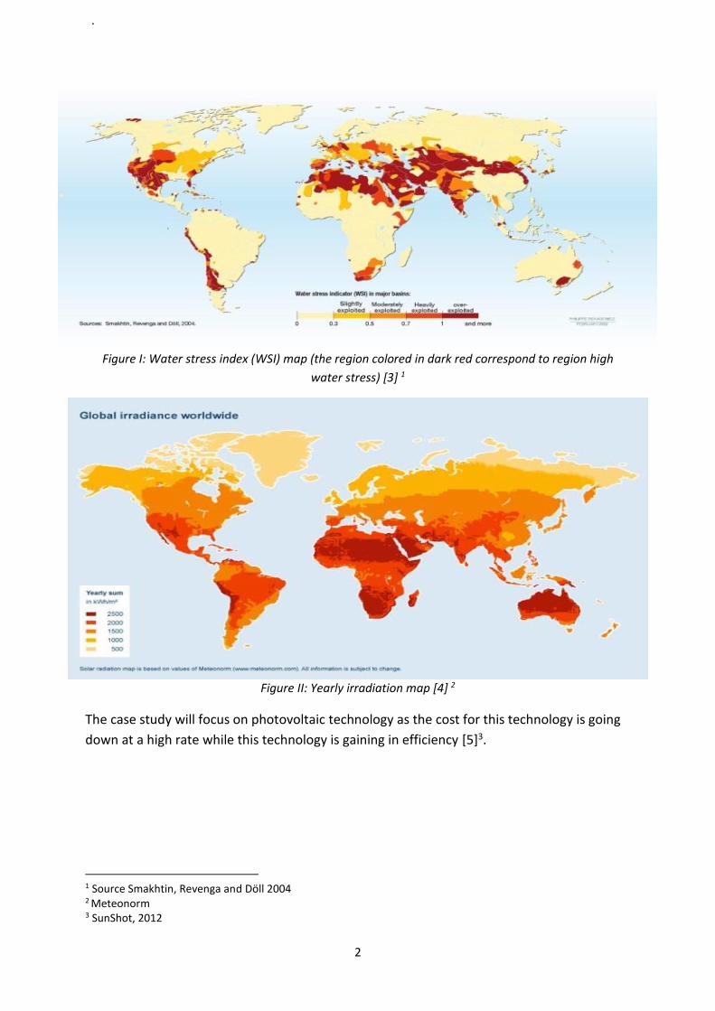
of M. Berrada and S. Caron. Figure I and Figure II show that regions where water stresses is

high, often have access to sea water and enjoy a large amount of solar irradiation. Morocco

faces a water stress issue and belongs to these regions [1]1. The desalination system used for

this case study is a reverse osmosis process which desalinates sea water and has a high energy

usage demand. This energy is wished to come from renewable energy in order to limit the

effect of greenhouse gas emissions caused by fossil fuels which in turn catalyze Climate

Change process [2]2.

1 Water desalination and solar in the Mediterranean Region, H. Ben Jallet Allal 2 M. Höök, 2012

.

2

Figure I: Water stress index (WSI) map (the region colored in dark red correspond to region high

water stress) [3] 1

Figure II: Yearly irradiation map [4] 2

The case study will focus on photovoltaic technology as the cost for this technology is going

down at a high rate while this technology is gaining in efficiency [5]3.

1 Source Smakhtin, Revenga and Döll 2004 2 Meteonorm 3 SunShot, 2012

.

3

First of all it has been studied which desalination process was the best for this case study. The

desalination process that was selected is a reverse osmosis process because the promoter of

the project has a few years of design experience with this technology. Moreover, this

technology represents about 50% of the market and its energy usage has considerably

decreased in the past decade [6]1 [7]2. A paper about the reverse osmosis desalination plant

has been written by M. Berrada and S. Caron where technical and economical features are

further discussed. See Appendix.

A first design case study has been completed by student groups at Högskolan Dalarna (Master

of Science in Solar Engineering). This design case study has been supervised by S. Caron. The

case study information and the students’ reports have been provided to start this thesis

project.

The project is located in Agadir (Morocco). The reverse osmosis desalination unit is designed

to supply fresh water for the irrigation system of a luxury hotel golf court. Currently the water

is extracted from a well located 15 km away from the hotel resort. However, the regulation

related to the watering of golf course in the region of Agadir has been reviewed. Soon the golf

courses of the Agadir region will need to get their water from the water treatment plant in

M’zar. This regulation forbids as well any water pumping from private wells, for this reason

the golf will not be allowed to use its well anymore. Because the quality of the water coming

from the treatment plant is not known yet, it might not be possible to spray this water over

the course if its quality is too low. Then two possibilities are feasible; use the water from the

drinking water grid or desalinate seawater, the ocean being only few hundred meters from

the golf.

In this case study we will look at the second option, and more particularly, the energy

production with photovoltaic cells for the desalination plant. The desalination plant will need

to provide all the water for the golf irrigation system (Figure III)

1 B Peñate et al, 2012 2 A. Soric et al, 2012

0

500

1000

1500

2000

2500

3000

3500

4000

4500

Jan Feb Mar Apr May Jun Jul Aug Sep Oct Nov Dec

Dai

ly c

on

sum

pti

on

| m

3 /d

ay

Figure III: Monthly water consumption profile (m3/day)

.

4

The cumulated water consumption is estimated at 1 080 000m3 per year. An energy analysis

focused on the desalination plant has been made earlier by Mehdi Berrada and Simon Caron

(see appendix) and shows that the desalination plant would consume 3.03kWh/m3 (see

appendix). This leads to an annual electricity usage of around 3.03GWh. On a monthly basis

the solar energy matches the load because more energy is needed during the summer than

during the winter. However, a slight shift is seen in figure IV and it is already predictable at

this stage that a higher shortage of energy for the month of August will be experienced. This

is the reason why this option is studied through this report. It would also follow the Moroccan

dynamic that aim for 2000MW for 2020 coming from solar energy [8]1

B) Objectives

The aims of this master project are (i) to design a photovoltaic (PV) power system to supply

most of the energy consumed by the reverse osmosis unit and (ii) to perform a techno-

economic analysis to select an optimized technology and sized solution.

1 Masen

5000

6000

7000

8000

9000

10000

11000

12000

13000

0.03

0.04

0.04

0.05

0.05

0.06

0.06

0.07

0.07

0.08

0.08

Jan Feb Mar Apr May Jun Jul Aug Sep Oct Nov Dec

Dai

ly e

ne

rgy

usa

ge ;

kW

h

Dai

ly I

rrad

iati

on

; kW

h/m

2.d

ay

Solar irradiation Load

Figure IV: Daily solar irradiation and daily energy usage over the year

.

5

I Project

- A) Boundary conditions

1-Location

The PV system would be located in Agadir (Morocco). The client is a golf course named “Le

Golf des Dunes”. The golf course is 101 hectares big and two fields of respectively 2 ha and 1

ha are available for the project (see figure 1.1). These fields are located 2 km from the

highway, 13km from the harbor and 20 km for the airport, which make any transport of

hardware easy.

Figure 1.1: Map of the golf court. In green the border of the golf, in red and yellow the two available

plots for the project [9]1

2-Economics

This part include general information about Moroccan economics linked to the project such

as interest rate, electricity and water cost for hotel resorts and support schemes for solar

energy project. The currency in Morocco is the Moroccan dirham (MAD) and is here assumed

to be worth 0.089€ (1€=11.2MAD)

It has been difficult to find reliable values for the interest rate but it often vary between 6%

and 10%. For these reason, some results will be express in function of the interest rate (figure

3.3 for example).

The cost of water in Morocco for this kind of system is fixed to 7.20 MAD/m3 or 0.643€/m3

[10]2. To this, it should be added a fix inclusive fee of 30MAD/trimester which corresponds

1 Google map 2 Office national de l’eau potable (ONEP)

.

6

approximately to 10€/year. Otherwise the VAT in not included in the m3 price; the VAT for the

water is 14% so that the final price is about 0,733€/m3.

The electricity price is divided in 3 three different periods; evening, night, day. The period

limits depend on the season, see Table 1.1.

Price category

Price (€/kWh)

Winter 1st Oct –31st Mar

Summer 1st Apr –30th Sept

P1 (evening, peak) 0.11 17h-22h 18h-23h

P2 (day) 0.07 7h-17h 7h-18h

P3 (night) 0.05 22h-7h 2h-7h

Table 1.1 Electricity pricing in Morocco

These prices already include a 14% VAT. To this proportional price, it should be included an

annual fee of 34€/kVA should be added [11]1. The maximum power needed for this study case

is 500kVA during the summer months. This will add 17000€ in the annual bill.

Then two reference systems can be set; (A) one which does not use the desalination plant but

use only the water from the drinking water system and (B) another one where the desalination

plant will be powered only by the grid.

The price for the system A take into account only the water consumption and the unit water

cost equals to 0.733€/m3. For the system B the prices had been calculated previously by M.

Berrada and S. Caron (see appendix) in their paper describing the desalination plant. During

the first ten years the water cost would be 0.86€/m3 and then 0.64€/m3. As the lifetime of a

desalination plant is expected to be 25 years, the average price of the water would be

0.737€/m3. As shown in the paper, during the plant lifetime, 45% of the water price is due to

the electricity cost. The aim of this project is to calculate the lifecycle cost of electricity for a

PV system and check if this system is economically competitive compared to systems A and B.

3-Solar resources

Agadir enjoys large solar irradiation which varies from 3.4kWh/m2/day in December, up to

7.6kWh/m2/day in June. The yearly irradiation is around 2.1MWh/m2/year. As can be

observed on figure 1.2 this is one of the best irradiation location in Africa and also on the

Earth. For this project the solar irradiation had been calculated from 4 different sources (Soda

service, NASA-SSE, RETscreen and PVGIS) and is showed in figure 1.4.

1 Office national de l’électrcité au Marco (ONE)

.

7

Figure 1.2 Solar yield (in kWh/m2/year) for Morocco looking at different scale [12]1

The temperature is also an important data because the hotter it gets, the worse the efficiency

of the panel is. Figure 1.3 shows this effect. For example, if the cell temperature is 25C, the

maximum power point (the green point in figure 1.3) has a voltage of around 17 Volts and a

current of around 2.7 Amps, therefore the power is around 46 Watts. But if the cell

temperature reaches 75 its maximum power point (the red point in figure 1.3) would be

around 36.5 Watts (13 Volts and 2.8 Amps). Moreover, this effect is shown in table 2.3 as

temperature coefficient for the PV panel.

Figure 1.3: The effect of temperature on I-V curve for PV module [13]2

1 Solargis 2 Photovoltaics for professionals. P.56

.

8

For similar reason, the wind speed is a value to take into consideration because it influence

the photovoltaic panels temperature therefore the values for wind speed are computed into

PVsyst (figure 1.4)

4-Load

The load had been calculated from the report about the desalination plant written by M.

Berrada and S. Caron (see appendix). In order to reduce as much as possible the cost from this

desalination plant, the reverse osmosis unit produces fresh water 24h a day. The irrigation

system only works from 8 pm to 5 am (night time, cycle duration: 9 hours). The fresh water is

produced by a reverse-osmosis desalination plant and consists of four reverse osmosis trains.

Each unit can produce 1000m3 a day or around 42m3 per hour. These units work only on their

full regime, therefore the partial load management is made by switching on one or several of

the four units. For example, during the winter the daily need of water is 2000m3 so 2 units will

work at the same time all day long (see table 1.2).

Figure 1.4: Irradiation, temperature and wind velocity computed into Pvsyst for the simulations

.

9

Time/Month Jan Feb Mar Apr May Jun Jul Aug Sep Oct Nov Dec 05:00

>> 06:00 83,3 83,3 83,3 125 125 167 167 167 125 125 83,3 83,3 06:00

>> 07:00 83,3 83,3 83,3 125 125 167 167 167 125 125 83,3 83,3 07:00

>> 08:00 83,3 83,3 125 125 167 167 167 167 167 125 125 83,3 08:00

>> 09:00 83,3 83,3 125 125 167 167 167 167 167 125 125 83,3 09:00

>> 10:00 83,3 83,3 125 125 167 167 167 167 167 125 125 83,3 10:00

>> 11:00 83,3 83,3 125 125 167 167 167 167 167 125 125 83,3 11:00

>> 12:00 83,3 83,3 125 125 167 167 167 167 167 125 125 83,3 12:00

>> 13:00 83,3 83,3 125 125 167 167 167 167 167 125 125 83,3 13:00

>> 14:00 83,3 83,3 125 125 167 167 167 167 167 125 125 83,3 14:00

>> 15:00 83,3 83,3 125 125 167 167 167 167 167 125 125 83,3 15:00

>> 16:00 83,3 83,3 125 125 167 167 167 167 167 125 125 83,3 16:00

>> 17:00 83,3 83,3 125 125 167 167 167 167 167 125 125 83,3 17:00

>> 18:00 83,3 83,3 125 125 167 167 167 167 167 125 125 83,3 18:00

>> 19:00 83,3 83,3 125 125 167 167 167 167 167 125 125 83,3 19:00

>> 20:00 83,3 83,3 83,3 125 125 167 167 167 125 125 83,3 83,3 20:00

>> 21:00 83,3 83,3 83,3 125 125 167 167 167 125 125 83,3 83,3 21:00

>> 22:00 83,3 83,3 83,3 125 125 167 167 167 125 125 83,3 83,3 22:00

>> 23:00 83,3 83,3 83,3 125 125 167 167 167 125 125 83,3 83,3 23:00

>> 00:00 83,3 83,3 83,3 125 125 167 167 167 125 125 83,3 83,3 00:00

>> 01:00 83,3 83,3 83,3 125 125 167 167 167 125 125 83,3 83,3 01:00

>> 02:00 83,3 83,3 83,3 125 125 167 167 167 125 125 83,3 83,3 02:00

>> 03:00 83,3 83,3 83,3 125 125 167 167 167 125 125 83,3 83,3 03:00

>> 04:00 83,3 83,3 83,3 125 125 167 167 167 125 125 83,3 83,3 04:00

>> 05:00 83,3 83,3 83,3 125 125 167 167 167 125 125 83,3 83,3

TOTAL m3: 2000 2000 2500 3000 3500 4000 4000 4000 3500 3000 2500 2000

Table 1.2: Daily clean water production depending on the time

The need in fresh water varies as showed in figure III.

The water produced during the day is stored in tank and then used by the spraying system.

Table 1.3 shows the water tank capacity in function of the time of the day and the month of

the year. Time/Month Jan Feb Mar Apr May Jun Jul Aug Sep Oct Nov Dec

05:00 >> 06:00 83 83 83 125 125 167 167 167 125 125 83 83 06:00 >> 07:00 167 167 167 250 250 333 333 333 250 250 167 167 07:00 >> 08:00 250 250 292 375 417 500 500 500 417 375 292 250 08:00 >> 09:00 333 333 417 500 583 667 667 667 583 500 417 333 09:00 >> 10:00 417 417 542 625 750 833 833 833 750 625 542 417 10:00 >> 11:00 500 500 667 750 917 1000 1000 1000 917 750 667 500 11:00 >> 12:00 583 583 792 875 1083 1167 1167 1167 1083 875 792 583 12:00 >> 13:00 667 667 917 1000 1250 1333 1333 1333 1250 1000 917 667 13:00 >> 14:00 750 750 1042 1125 1417 1500 1500 1500 1417 1125 1042 750 14:00 >> 15:00 833 833 1167 1250 1583 1667 1667 1667 1583 1250 1167 833 15:00 >> 16:00 917 917 1292 1375 1750 1833 1833 1833 1750 1375 1292 917 16:00 >> 17:00 1000 1000 1417 1500 1917 2000 2000 2000 1917 1500 1417 1000 17:00 >> 18:00 1083 1083 1542 1625 2083 2167 2167 2167 2083 1625 1542 1083 18:00 >> 19:00 1167 1167 1667 1750 2250 2333 2333 2333 2250 1750 1667 1167 19:00 >> 20:00 1250 1250 1750 1875 2375 2500 2500 2500 2375 1875 1750 1250 20:00 >> 21:00 1111 1111 1556 1667 2111 2222 2222 2222 2111 1667 1556 1111 21:00 >> 22:00 972 972 1361 1458 1847 1944 1944 1944 1847 1458 1361 972 22:00 >> 23:00 833 833 1167 1250 1583 1667 1667 1667 1583 1250 1167 833 23:00 >> 00:00 694 694 972 1042 1319 1389 1389 1389 1319 1042 972 694 00:00 >> 01:00 556 556 778 833 1056 1111 1111 1111 1056 833 778 556 01:00 >> 02:00 417 417 583 625 792 833 833 833 792 625 583 417 02:00 >> 03:00 278 278 389 417 528 556 556 556 528 417 389 278 03:00 >> 04:00 139 139 194 208 264 278 278 278 264 208 194 139 04:00 >> 05:00 0 0 0 0 0 0 0 0 0 0 0 0

Table 1.3: Hourly capacity (in m3) of the water tank during a day.

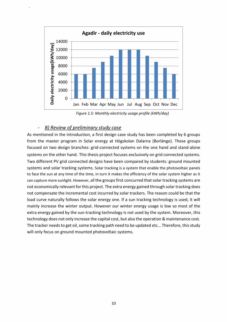
Table 1.3 is built knowing that the irrigation takes place between 8pm and 5am, that the flow

is constant and that the water consumption follows the table 1.2. As we see in table 1.3 the

water tank needs to be at least 2500m3 large. The desalination plant has a specific energy

usage of 3kWh/m3, this leads the electric usage profile in figure 1.5.

.

10

Figure 1.5: Monthly electricity usage profile (kWh/day)

- B) Review of preliminary study case

As mentioned in the introduction, a first design case study has been completed by 6 groups

from the master program in Solar energy at Högskolan Dalarna (Borlänge). These groups

focused on two design branches: grid-connected systems on the one hand and stand-alone

systems on the other hand. This thesis project focuses exclusively on grid connected systems.

Two different PV grid connected designs have been compared by students: ground mounted

systems and solar tracking systems. Solar tracking is a system that enable the photovoltaic panels

to face the sun at any time of the time, in turn it makes the efficiency of the solar system higher as it

can capture more sunlight. However, all the groups first concurred that solar tracking systems are

not economically relevant for this project. The extra energy gained through solar tracking does

not compensate the incremental cost incurred by solar trackers. The reason could be that the

load curve naturally follows the solar energy one. If a sun tracking technology is used, it will

mainly increase the winter output. However our winter energy usage is low so most of the

extra energy gained by the sun-tracking technology is not used by the system. Moreover, this

technology does not only increase the capital cost, but also the operation & maintenance cost.

The tracker needs to get oil, some tracking path need to be updated etc... Therefore, this study

will only focus on ground mounted photovoltaic systems.

0

2000

4000

6000

8000

10000

12000

14000

Jan Feb Mar Apr May Jun Jul Aug Sep Oct Nov DecDai

ly e

lect

rici

ty u

sage

[kW

h/d

ay]

Agadir - daily electricity use

.

11

II Method

- A) Scope of simulation

To simulate the photovoltaic power plant, the software PVsyst has been used. This software

is developed by Geneva University since 1992 [14]1. It is a very complete software and

worldwide used for every photovoltaic systems. Every simulation includes seven steps that

we will be explained.

1-Project

In the project part, the geographic location is defined and the solar resources for the project

are computed. PVsyst includes its own solar data for some locations, but in this project

customized values are used. Those had been calculated previously for the student reports by

S. Caron2 and are based on four different sources: Soda service, NASA-SSE, RETscreen and

PVGIS (see figure 1.4).

2-Orientation

In the orientation part, the direction the panels are facing (south for this study case), and the

angle the panels will form with the ground (the inclination or tilt angle) are set (see figure 2.2).

As it is shown in the part boundary condition part (I-A) the energy usage between winter time

and summer time is big, otherwise at this latitude (closer to the equator), the solar resource

gap between winter and summer is not that big. That is the reason why the inclination needs

to be optimized for the summer months.

Figure 2.1: Optimum tilt angle for northern latitudes [15]3

1 www.pvsyst.com/en 2 Simon Caron was in charge to introduce the project to the master program in Solar energy from Högskolan Dalarna which did preliminary case study. Therefore inputs to the projects such as solar irradiation or temperature were already available for this project. 3 Photovoltaics for professionals. P.78

.

12

According to figure 2.1 the inclination should be between 5 and 10 degrees. Otherwise, with

an inclination too low, the dirt on the panel would be a problem because it will not be steep

enough to self-wash. So the inclination is decided to be 15 degree, figure 2.2. Moreover, on a

technical point of view, a pitch angle of 15 degrees matches the installation requirements

because the support system offers this possibility (see part II-B-3).

3-Horizon

The horizon part consists to simulate the horizon line in order to know how much useful sun

is actually available. The red line corresponds to obstacles around the solar field. It represents

mainly distant trees. The blue line corresponds to the auto-shading of the modules (see next

part: 4-Near shading part).

4-Near shading

This part of the software simulates the effect of shadow from close objects (less than 50

meters). For this part a 3D simulation is drawn for the system and then different objects such

as house, tree, and fences are added. For this case, it has been tried to simulate the closest

trees and the fence that will prevent against robbery, but this was too many objects for the

software or the computer (which crashed), so instead it has been tried to integrate these in

the horizon line. As we see on figure 2.6b, there are no trees on the west side of the solar

field. Moreover, the golf resort could cut down trees if needed.

Figure 2.2: Orientation and inclination parameters in PVsyst

Figure 2.3: Horizon simulated into PVsyst

.

13

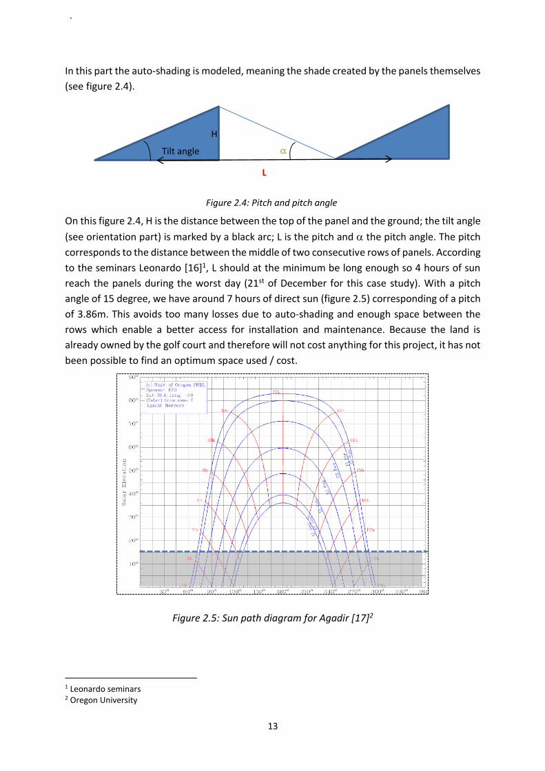
In this part the auto-shading is modeled, meaning the shade created by the panels themselves

(see figure 2.4).

On this figure 2.4, H is the distance between the top of the panel and the ground; the tilt angle

(see orientation part) is marked by a black arc; L is the pitch and the pitch angle. The pitch

corresponds to the distance between the middle of two consecutive rows of panels. According

to the seminars Leonardo [16]1, L should at the minimum be long enough so 4 hours of sun

reach the panels during the worst day (21st of December for this case study). With a pitch

angle of 15 degree, we have around 7 hours of direct sun (figure 2.5) corresponding of a pitch

of 3.86m. This avoids too many losses due to auto-shading and enough space between the

rows which enable a better access for installation and maintenance. Because the land is

already owned by the golf court and therefore will not cost anything for this project, it has not

been possible to find an optimum space used / cost.

Figure 2.5: Sun path diagram for Agadir [17]2

1 Leonardo seminars 2 Oregon University

Tilt angle

H

L

Figure 2.4: Pitch and pitch angle

example

.

14

Figure 2.5 is a sun path diagram which give the position of the sun for a particular place. The

blue curved lines represent the sun path for a single day. For example, the highest line

represent June 21st. This day in Agadir, the sun rise from the horizon around 5am and set at

7pm. However, in practice the panels cannot caught sunlight if the solar elevation is lower

than 15 which represent the pitch angle discussed previously. Therefore, in practice the

sunlight will able to reach the panels (for June 21st) from 6.30am till 5.30pm.

On figure 2.6 b the red space represents the available area equals to 2 ha. The green line is

the golf border and in grey/yellow the existing road. This site is only 2km from the closest

highway. With a pitch of 3.86m, so 1.932m between every rows, and taking into account space

taking by the road and the building housing all the technical hardware, this plot could contain

9332 panels (table 2.1). The panel size is given in next part: technical data. The panels will be

positioned is portrait format, with two panels per row.

Figure 2.6a corresponds to the 2 ha plot available for this project and its close surrounding. It

has been modeled with Microsoft excel and had been used to estimate the maximum number

of panels that the plot could contain. The dark red areas correspond to cleared field. The green

area on the right side corresponds to woodland.

The remaining surface corresponds to the available area available for the project. Within this

area, the brown bands are 10m wide roads where trucks could drive in order to deliver the

panels and other hardware during the construction or maintenance. These roads are planned

on the east side of the plot in order to decrease the shadow effect from woodland located on

the east hand. On the top north part, the dark brown rectangle is the technical house where

the inverters and all the hardware equipment will be located. The building could measure up

to 20m*10m. The four colorful areas (1, 2, 3 and 4) are the areas where the photovoltaic

panels will be. Finally the 6 dark orange bands show the width in term of panel. For instance,

Figure 2.6a: Outline of the 2ha plot. Figure 2.6b: Satellite view of the 2ha plot

(google map)

.

15

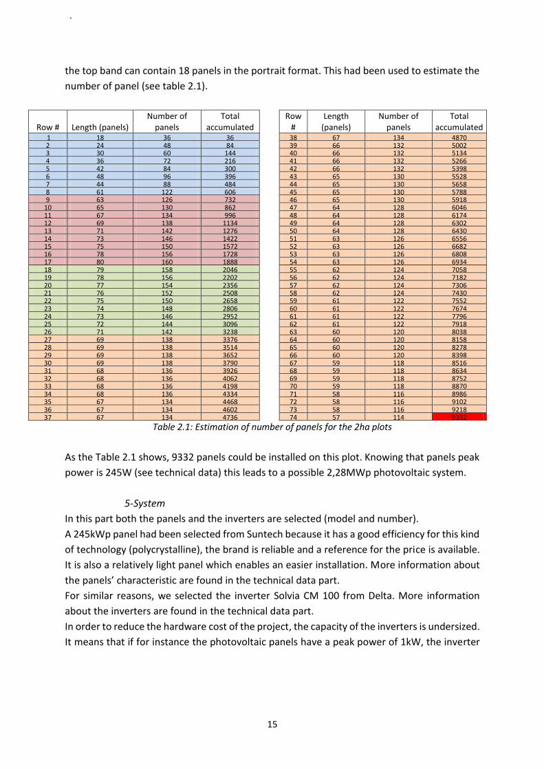
the top band can contain 18 panels in the portrait format. This had been used to estimate the

number of panel (see table 2.1).

Row # Length (panels) Number of

panels Total

accumulated Row

# Length

(panels) Number of

panels Total

accumulated 1 18 36 36 38 67 134 4870 2 24 48 84 39 66 132 5002 3 30 60 144 40 66 132 5134 4 36 72 216 41 66 132 5266 5 42 84 300 42 66 132 5398 6 48 96 396 43 65 130 5528 7 44 88 484 44 65 130 5658 8 61 122 606 45 65 130 5788 9 63 126 732 46 65 130 5918

10 65 130 862 47 64 128 6046 11 67 134 996 48 64 128 6174 12 69 138 1134 49 64 128 6302 13 71 142 1276 50 64 128 6430 14 73 146 1422 51 63 126 6556 15 75 150 1572 52 63 126 6682 16 78 156 1728 53 63 126 6808 17 80 160 1888 54 63 126 6934 18 79 158 2046 55 62 124 7058 19 78 156 2202 56 62 124 7182 20 77 154 2356 57 62 124 7306 21 76 152 2508 58 62 124 7430 22 75 150 2658 59 61 122 7552 23 74 148 2806 60 61 122 7674 24 73 146 2952 61 61 122 7796 25 72 144 3096 62 61 122 7918 26 71 142 3238 63 60 120 8038 27 69 138 3376 64 60 120 8158 28 69 138 3514 65 60 120 8278 29 69 138 3652 66 60 120 8398 30 69 138 3790 67 59 118 8516 31 68 136 3926 68 59 118 8634 32 68 136 4062 69 59 118 8752 33 68 136 4198 70 59 118 8870 34 68 136 4334 71 58 116 8986 35 67 134 4468 72 58 116 9102 36 67 134 4602 73 58 116 9218 37 67 134 4736 74 57 114 9332

Table 2.1: Estimation of number of panels for the 2ha plots

As the Table 2.1 shows, 9332 panels could be installed on this plot. Knowing that panels peak

power is 245W (see technical data) this leads to a possible 2,28MWp photovoltaic system.

5-System

In this part both the panels and the inverters are selected (model and number).

A 245kWp panel had been selected from Suntech because it has a good efficiency for this kind

of technology (polycrystalline), the brand is reliable and a reference for the price is available.

It is also a relatively light panel which enables an easier installation. More information about

the panels’ characteristic are found in the technical data part.

For similar reasons, we selected the inverter Solvia CM 100 from Delta. More information

about the inverters are found in the technical data part.

In order to reduce the hardware cost of the project, the capacity of the inverters is undersized.

It means that if for instance the photovoltaic panels have a peak power of 1kW, the inverter

.

16

could have a capacity lower (to a certain extent) than 1kWHowever this do not harm the

inverters [18]1.

The size of the project, or in other words the number of panels and inverters, depends of the

scenario and are dealt with in the system design part.

6-Module layout

This section deals with the interconnections of the panels. It has to be done in an efficient way

to avoid the so called “hot spot”. When several cells (or panels) are connected in series, the

current is imposed by the one with the lowest, which correspond to the one with the least

irradiation or a defaulting cell, (see figure 2.7)

Figure 2.7: Hot spot phenomenon [19]2 [20]3

Otherwise, with big system like this, it takes a long time to do it, therefore this will not be done

in this paper. One of the reason is that no near shading obstacle could have been simulated

with PVsyst so it will not make big loses at all in the calculations. It is however advised to

regroup the modules in a way that if one module in shaded, it is most likely that all the other

modules from the same string are shaded as well.

7-Simulation

Once all this parameters are filled, the simulation of our system can be run on PVsyst. The

focus is hold on monthly results such as net energy available, energy used by the system

1 S. Chen et al, 2013 2 Applied photovoltaics. P.77 3 Photovoltaics for professionals. P.129

.

17

energy needed from the grid, and energy given to the grid. With this figures it will be possible

then to calculate the solar fraction.

Two scenario will be studied; a system with monthly net metering and a system without.

However, only the results for the net metering are exposed in this paper. With the monthly

net metering the client pay the difference between the production and the energy usage. For

example, if a home system produces 200 kWh during March and that the household consume

250kWh during the same period, then the client will pay to the grid the price for 50kWh.

Otherwise, if it produces more than it consumes, then the owner will not get paid from the

grid owner, so the overproduction is seen as lost.

The monthly net metering scenario is studied because looking at the load (table 2.2) it is

impossible to reach a solar fraction close to 100% because of the simple reason that the

system will not be able to produce energy during the night time while the load needs energy

24 hours a day.

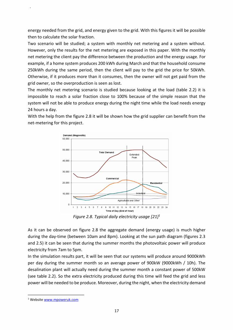
With the help from the figure 2.8 it will be shown how the grid supplier can benefit from the

net-metering for this project.

Figure 2.8. Typical daily electricity usage [21]1

As it can be observed on figure 2.8 the aggregate demand (energy usage) is much higher

during the day-time (between 10am and 8pm). Looking at the sun path diagram (figures 2.3

and 2.5) it can be seen that during the summer months the photovoltaic power will produce

electricity from 7am to 5pm.

In the simulation results part, it will be seen that our systems will produce around 9000kWh

per day during the summer month so an average power of 900kW (9000kWh / 10h). The

desalination plant will actually need during the summer month a constant power of 500kW

(see table 2.2). So the extra electricity produced during this time will feed the grid and less

power will be needed to be produce. Moreover, during the night, when the electricity demand

1 Website www.mpoweruk.com

.

18

is lower, then our plant will need electricity. As a result, the power plant (mainly coal in

Morocco) will run on a more constant regime because the photovoltaic plant will partly reduce

the day-time peak demand and more electricity will be needed during the night. This is part

of the energy management and it is known that switching on and off coal power plant is not

that efficient and create problems for the materials [22]1.

Time/Month Jan Feb Mar Apr May Jun Jul Aug Sep Oct Nov Dec

05:00 >> 06:00 250 250 250 375 375 500 500 500 375 375 250 250

06:00 >> 07:00 250 250 250 375 375 500 500 500 375 375 250 250

07:00 >> 08:00 250 250 375 375 500 500 500 500 500 375 375 250

08:00 >> 09:00 250 250 375 375 500 500 500 500 500 375 375 250

09:00 >> 10:00 250 250 375 375 500 500 500 500 500 375 375 250

10:00 >> 11:00 250 250 375 375 500 500 500 500 500 375 375 250

11:00 >> 12:00 250 250 375 375 500 500 500 500 500 375 375 250

12:00 >> 13:00 250 250 375 375 500 500 500 500 500 375 375 250

13:00 >> 14:00 250 250 375 375 500 500 500 500 500 375 375 250

14:00 >> 15:00 250 250 375 375 500 500 500 500 500 375 375 250

15:00 >> 16:00 250 250 375 375 500 500 500 500 500 375 375 250

16:00 >> 17:00 250 250 375 375 500 500 500 500 500 375 375 250

17:00 >> 18:00 250 250 375 375 500 500 500 500 500 375 375 250

18:00 >> 19:00 250 250 375 375 500 500 500 500 500 375 375 250

19:00 >> 20:00 250 250 250 375 375 500 500 500 375 375 250 250

20:00 >> 21:00 250 250 250 375 375 500 500 500 375 375 250 250

21:00 >> 22:00 250 250 250 375 375 500 500 500 375 375 250 250

22:00 >> 23:00 250 250 250 375 375 500 500 500 375 375 250 250

23:00 >> 00:00 250 250 250 375 375 500 500 500 375 375 250 250

00:00 >> 01:00 250 250 250 375 375 500 500 500 375 375 250 250

01:00 >> 02:00 250 250 250 375 375 500 500 500 375 375 250 250

02:00 >> 03:00 250 250 250 375 375 500 500 500 375 375 250 250

03:00 >> 04:00 250 250 250 375 375 500 500 500 375 375 250 250

04:00 >> 05:00 250 250 250 375 375 500 500 500 375 375 250 250

- B) Technical data : market survey

1-Panels

The module STP245 – 20/Wd [26] from the company Suntech has been

chosen because of its good efficiency (15.1%), the fact the company is

reliable (one of the biggest PV supplier of both PV cells and PV modules)

[23]2 [24]3 [25]4, it is included in the simulation program database and also

because prices has been found for this module. It is a polycrystalline panel.

One module contains 60 cells. It is already equipped with a junction box

with make the connection easier and faster. Three bypass diodes per

module are included which reduces the hot spot effect (see figure

2.7).

1 Report on coal-fired power by the Energy Technology System Analysis Programme 2 www.pv-tech.org 3 www.pvinsights.com 4 www.solarbuzz.com

Figure 2.9: STP245-20/Wd

module

Table 2.2: Electric power (kWh) needed for the desalination plant hour by hour in function of the month

.

19

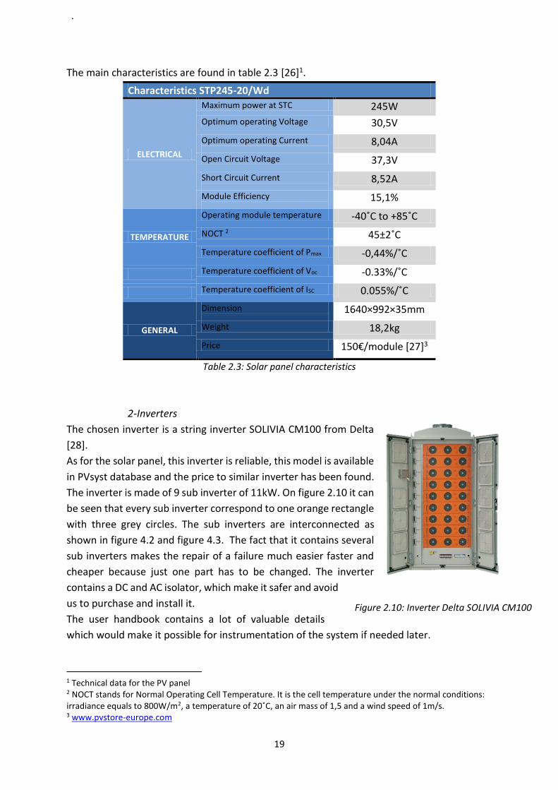
The main characteristics are found in table 2.3 [26]1.

Characteristics STP245-20/Wd

ELECTRICAL

Maximum power at STC 245W

Optimum operating Voltage 30,5V

Optimum operating Current

8,04A

Open Circuit Voltage 37,3V

Short Circuit Current

8,52A

Module Efficiency

15,1%

TEMPERATURE

Operating module temperature -40˚C to +85˚C

NOCT 2 45±2˚C

Temperature coefficient of Pmax -0,44%/˚C

Temperature coefficient of Voc -0.33%/˚C

Temperature coefficient of ISC 0.055%/˚C

GENERAL

Dimension

1640×992×35mm

Weight 18,2kg

Price 150€/module [27]3

Table 2.3: Solar panel characteristics

2-Inverters

The chosen inverter is a string inverter SOLIVIA CM100 from Delta

[28].

As for the solar panel, this inverter is reliable, this model is available

in PVsyst database and the price to similar inverter has been found.

The inverter is made of 9 sub inverter of 11kW. On figure 2.10 it can

be seen that every sub inverter correspond to one orange rectangle

with three grey circles. The sub inverters are interconnected as

shown in figure 4.2 and figure 4.3. The fact that it contains several

sub inverters makes the repair of a failure much easier faster and

cheaper because just one part has to be changed. The inverter

contains a DC and AC isolator, which make it safer and avoid

us to purchase and install it.

The user handbook contains a lot of valuable details

which would make it possible for instrumentation of the system if needed later.

1 Technical data for the PV panel 2 NOCT stands for Normal Operating Cell Temperature. It is the cell temperature under the normal conditions: irradiance equals to 800W/m2, a temperature of 20˚C, an air mass of 1,5 and a wind speed of 1m/s. 3 www.pvstore-europe.com

Figure 2.10: Inverter Delta SOLIVIA CM100

.

20

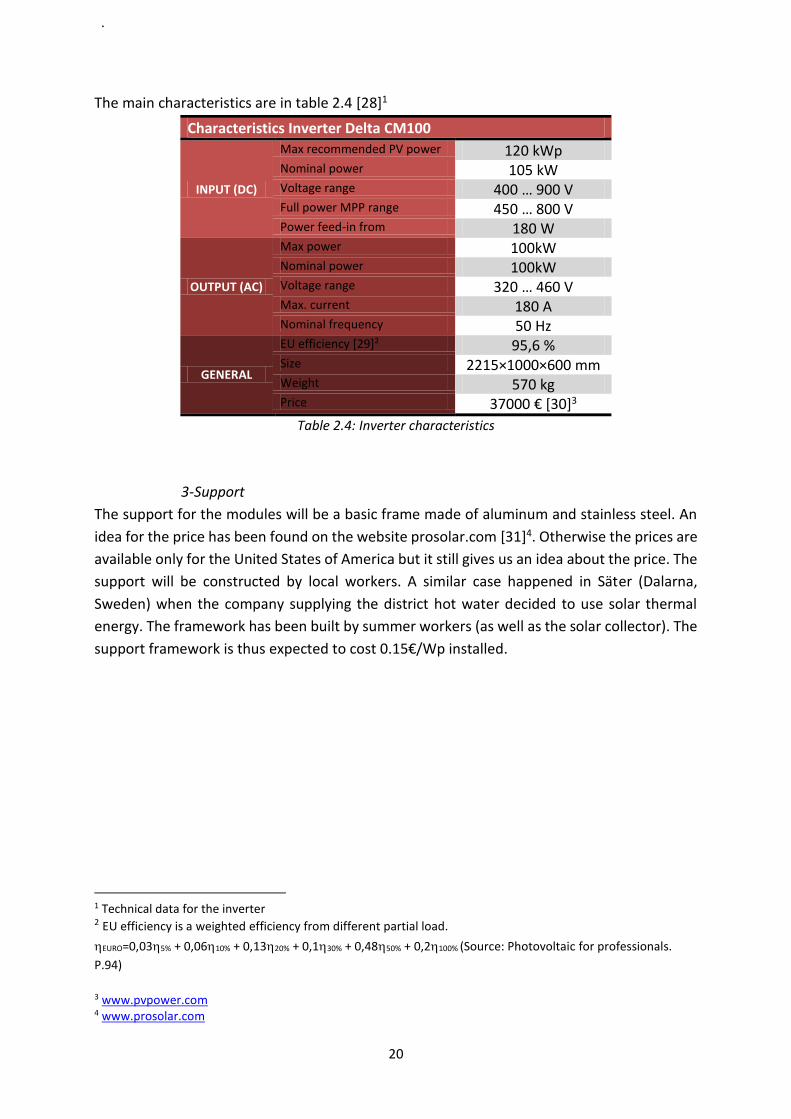
The main characteristics are in table 2.4 [28]1

Characteristics Inverter Delta CM100

INPUT (DC)

Max recommended PV power 120 kWp Nominal power 105 kW Voltage range 400 … 900 V Full power MPP range 450 … 800 V Power feed-in from 180 W

OUTPUT (AC)

Max power 100kW Nominal power 100kW Voltage range 320 … 460 V Max. current 180 A Nominal frequency 50 Hz

GENERAL

EU efficiency [29]2 95,6 % Size 2215×1000×600 mm Weight 570 kg Price 37000 € [30]3

Table 2.4: Inverter characteristics

3-Support

The support for the modules will be a basic frame made of aluminum and stainless steel. An

idea for the price has been found on the website prosolar.com [31]4. Otherwise the prices are

available only for the United States of America but it still gives us an idea about the price. The

support will be constructed by local workers. A similar case happened in Säter (Dalarna,

Sweden) when the company supplying the district hot water decided to use solar thermal

energy. The framework has been built by summer workers (as well as the solar collector). The

support framework is thus expected to cost 0.15€/Wp installed.

1 Technical data for the inverter 2 EU efficiency is a weighted efficiency from different partial load.

EURO=0,035% + 0,0610% + 0,1320% + 0,130% + 0,4850% + 0,2100% (Source: Photovoltaic for professionals.

P.94)

3 www.pvpower.com 4 www.prosolar.com

.

21

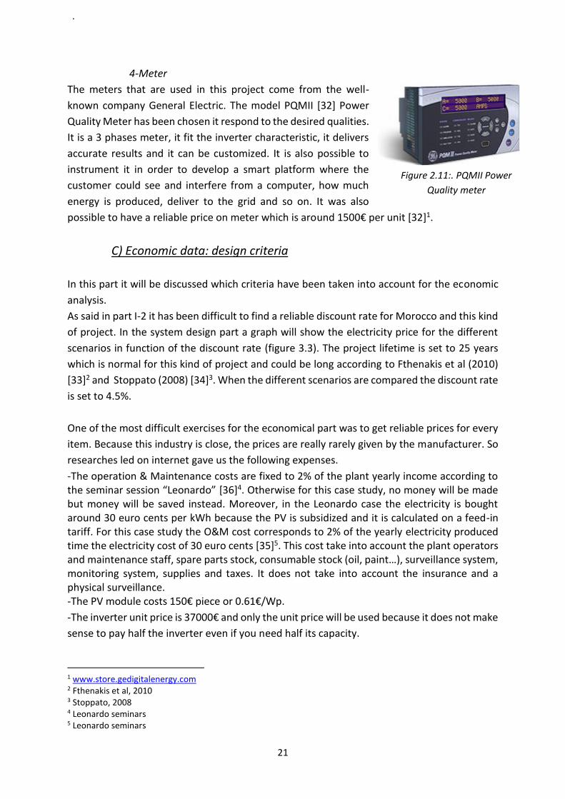
4-Meter

The meters that are used in this project come from the well-

known company General Electric. The model PQMII [32] Power

Quality Meter has been chosen it respond to the desired qualities.

It is a 3 phases meter, it fit the inverter characteristic, it delivers

accurate results and it can be customized. It is also possible to

instrument it in order to develop a smart platform where the

customer could see and interfere from a computer, how much

energy is produced, deliver to the grid and so on. It was also

possible to have a reliable price on meter which is around 1500€ per unit [32]1.

C) Economic data: design criteria

In this part it will be discussed which criteria have been taken into account for the economic

analysis.

As said in part I-2 it has been difficult to find a reliable discount rate for Morocco and this kind

of project. In the system design part a graph will show the electricity price for the different

scenarios in function of the discount rate (figure 3.3). The project lifetime is set to 25 years

which is normal for this kind of project and could be long according to Fthenakis et al (2010)

[33]2 and Stoppato (2008) [34]3. When the different scenarios are compared the discount rate

is set to 4.5%.

One of the most difficult exercises for the economical part was to get reliable prices for every

item. Because this industry is close, the prices are really rarely given by the manufacturer. So

researches led on internet gave us the following expenses.

-The operation & Maintenance costs are fixed to 2% of the plant yearly income according to the seminar session “Leonardo” [36]4. Otherwise for this case study, no money will be made but money will be saved instead. Moreover, in the Leonardo case the electricity is bought around 30 euro cents per kWh because the PV is subsidized and it is calculated on a feed-in tariff. For this case study the O&M cost corresponds to 2% of the yearly electricity produced time the electricity cost of 30 euro cents [35]5. This cost take into account the plant operators and maintenance staff, spare parts stock, consumable stock (oil, paint…), surveillance system, monitoring system, supplies and taxes. It does not take into account the insurance and a physical surveillance. -The PV module costs 150€ piece or 0.61€/Wp.

-The inverter unit price is 37000€ and only the unit price will be used because it does not make

sense to pay half the inverter even if you need half its capacity.

1 www.store.gedigitalenergy.com 2 Fthenakis et al, 2010 3 Stoppato, 2008 4 Leonardo seminars 5 Leonardo seminars

Figure 2.11:. PQMII Power

Quality meter

.

22

-As for the inverter, the meter price will only be mentioned per unit. One meter will be

connected to one inverter and the cost of the meter is 1500€.

-For the remaining hardware equipment the price will be expressed in €/kWp installed and

thus is dependent of the PV size. The hardware part includes the following items.

-The cable cost has been according to a rough drawing and is about 15€/kWp

installed. The linear cost for the cable is around 2€/m and two different section would be used;

6mm2 and 3mm2.

-The combiner boxes allow easier and safer connections between the modules.

The unit price for such a combiner box with 5 inputs is 82€ [36]1. With the inverter we use for

this project, 7 combiner boxes are needed for each inverter (see figure 4.3) thus the price is

around 3,5€/kWp installed.

-The support for the modules costs 150€/kWp (see part II-B-4)

The different prices are summarized in table 2.5.

Price Unit

Modules 150€ per unit Inverters 37000€ per unit Meters 1500€ per unit Hardware 168,5€ per kWp installed O&M Cost 2% of yearly income

The economic analysis does not include insurance, civil work, engineering work and

transportation. During the civil work, trees will be cut so some profit could be made but it is

not include in the economic analysis either. As well as the dismantling costs, this would give

extra benefits for the project after the plant lifetime.

1 Price for combiner box

Table 2.5: Pricing summarization

.

23

III System Design

A) Different scenarios

The different scenarios only differ in term on size (kWp). They all use the same panels, the

same mounting structure so the same tilt angle, the same pitch (distance between two

consecutive rows) and the same inverters.

The size of each scenario is determined by the inverter capacity. Because the inverters are

costly we will use the full capacity of every inverter. As it will be shown later (part IV), on each

inverter, 25 strings of 20 panels in series can be connected. So every inverter is connected to

500 panels. To reduce the capital cost without reducing the output of the system, the capacity

of the inverters is slightly undersize. This means that every inverter has an input capacity

slightly higher than its nominal capacity. However this overpowering of the inverters will not

harm the inverters. One of the reasons is that when the sun is shining the most, the

temperature rises which make the PV module less efficient, in turn the module will not deliver

its maximum power (see figure 2.1). Another reason is that inverters can handle a small

overpowering without altering its efficiency.

Eleven different scenarios have been simulated. The first one includes 10 inverters and 5000

panels, the second 11 inverters and 5500 panels and so on up to the last scenario which

includes 20 inverters and 10000 panels in total. The connections between the modules and

the inverters are explained in the fourth part “Detailed design”.

All other parameters such as orientation, tilt angle, pitch, horizon, etc… are discussed in the

method part and remain the same for the every scenario.

B) Simulation results

The raw results of the different scenarios are given in figure 3.1 .

.

24

a: 1225kWp b: 1348kWp

e: 1715kWp d: 1593kWp

g: 1960kWp

f: 1838kWp

i: 2328kWp

g: 2083kWp h: 2205kWp

j: 2450kWp

c: 1470kWp

Legend

Figure 3.1: Presentation the simulations for the eleven scenarios (Monthly energy in kWh)

.

25

As most of the calculations are based on these graphs, they will be analyzed in depth. All the

calculation are done on the monthly net metering basis (see part II-A-7). The red line

corresponds to the electric load and is identical for every scenario as the amount of energy

needed to desalinate salt water is the same. This line is similar to the figure 1.6 in the project

part except that the graph corresponds to the daily load while figure 3.1 corresponds to the

monthly load. The blue line called “Solar” shows the system energy output available. It

corresponds to the electricity that is available for the system and that is produced by the

photovoltaic power plant. The green area called “E used” is the solar energy used by the

system to produce fresh water. The violet area called “From the grid” is the energy coming

from the grid when not enough electricity is produced during the month. Finally the blue area

“To grid” is the surplus electricity which is fed to the grid.

C) Tools for decision making

For this project different tools are used. Those tools will help to decide what scenario is the

most suitable. Firstly the problem will be analyzed on a pure economical perspective and

secondly through a tool that had been implemented for this particular project.

1- Economic perspective

The levelized cost of energy is a tool often used for this kind of project. The inputs for this are

the capital cost, the Operation and Maintenance costs (O&M), the useful production of

electricity, the discount rate and the expected lifetime of the project (t). By useful production

of electricity it is meant the electricity produced by the PV system and consumed by the

desalination plant, therefore the surplus of electricity given to the grid is seen here as waste

energy. The project lifetime is set to 25 years and the discount rate is set as unknown. The

formula shown in figure 3.2 has been computed with the discount rate set as unknown, and

figure 3.3 shows the results.

Capital Cost × Discount rate 1

1-(1+discount rate)-t) + O&M cost useful production (kWh) ×

Figure 3.2 Formula to calculate the levelized cost of electricity

Levelized cost of electrcity

.

26

The lowest levelized costs of electricity are for the projects with the lowest capacity. The

dotted lines show the actual price for electricity in Morocco (see I-A-2). For this kind of project,

discount rate can vary between 5 to 10% [37]1 [38]2.

1 D. Zejli et al. 2004 2 G. Notton et al. 1998

Figure 3.3 Levelized cost of electricity for the 11 scenarios in function of the discount rate

.

27

For a set discount rate equal to 4.5%, figure 3.4 shows the levelized cost of electricity of the

eleven different scenarios and their capital cost.

One of the problems for this kind of approach is that it does not take into account the entire

problem into consideration, for instance it does not include the electricity bill that remains to

be paid. As there are three different tariffs for electricity it is difficult to decide which tariff to

take into consideration. The common sense will be to decide to choose the night tariff because

we know that we will not produce so in turn the system will consume electricity from the grid.

However, in this paper we assume that a monthly net metering is used, therefore one of the

conditions in order to get this net metering will be to pay the peak price for the electricity

deficit. To leave full option for decision makers, the three options have been investigated;

paying only at low tariff (night), medium (day) or peak tariff. The results are shown in figure

3.5.

Figure 3.4 Levelized cost of electricity and capital costs of the 11 scenarios

.

28

What is seen in figure 3.5 is that the lowest total yearly cost for powering the desalination

plant depends on the electricity price. If all the electricity coming from the grid is paid at the

low tariff, then the 1593 kWp project seems economically the most interesting. If the medium

tariff is chosen instead, the 1712 kWp project is the least expensive. Finally if the peak tariff is

charged for the electricity coming from the grid the 1960 kWp project should be chosen

according to this method.

In this paper the price of electricity is assumed to remain the same for the 25 years. However

it is most likely that prices will increase and it is reasonable to make a decision looking at the

peak tariff scenario. On figure 3.5 it can also be seen that a trend appears; the more expensive

the electricity price is, the more interesting bigger project become.

2- New perspective

In this part the economics will be ignored and a new simple tool will be used to compare the

different scenarios. What is often expected for PV projects is to reach a high solar fraction,

meaning aiming for the higher share of solar electricity in the system. This solar fraction is

simply the ratio between the solar energy in the system and the overall energy in the system.

Another point that is often neglected is the wasted energy. By wasted energy it is meant extra

energy that is produced but that the load cannot consume. To sum up, we want a high solar

fraction and a low wasted solar energy fraction.

Figure 3.5: Yearly cost for the solar power plant and cost of electricity needed for the desalination process

.

29

A simple mathematical formula has been used to show which scenario fulfill the most these

two criteria: / (1+) where is the solar fraction, and the solar energy wasted fraction.

This ratio is calculated for one year.

To this basic formula a weighting coefficient is applied to ( from ¼ to 4), depending how the

decision makers want to incorporate the wasted solar energy fraction into the final decision.

If the coefficient 4 is applied, then it means that the component “wasted solar energy” is very

important and the opposite is true if the coefficient ¼ is used. Figure 3.7 shows the results.

In this table, only figures within the same column can be compared as different columns use

different formulas (different coefficients). If a great solar fraction is prioritized the decision

makers should look at the right hand side of the table, in the other hand if the decision makers

want to minimize the solar energy wasted they should focus on the left hand side of the table.

The higher ratio in a column corresponds to the best alternative; therefore the green colored

cells correspond to the best alternatives. We can see an obvious trend that scenarios with high

capacity should be prioritized if a great solar fraction is expected while smaller capacity

projects waste less solar energy.

This tool makes sense if the investor is private and do not own the electrical grid, or if there is

no feed-in tariff.

= solar electricity used by the system (E used)

load

= Electricity yield to the grid (To grid)

Total solar electricity produced

(Solar) Figure 3.6: Formulas for the solar fraction and solar energy wasted fraction calculations

1225kWp 0,630 0,630 0,630 0,630 0,630 0,630 0,630

1348 kWp 0,693 0,693 0,693 0,693 0,693 0,693 0,693

1470 kWp 0,738 0,741 0,745 0,749 0,751 0,751 0,751

1593 kWp 0,776 0,784 0,793 0,801 0,816 0,807 0,808

1715kWp 0,764 0,785 0,807 0,831 0,843 0,847 0,849

1838 kWp 0,727 0,762 0,801 0,844 0,867 0,875 0,879

1960 kWp 0,687 0,734 0,788 0,850 0,884 0,897 0,903

2083 kWp 0,651 0,706 0,772 0,851 0,897 0,914 0,922

2205 kWp 0,617 0,679 0,755 0,850 0,907 0,927 0,938

2328 kWp 0,586 0,652 0,736 0,844 0,912 0,936 0,949

2450 kWp 0,547 0,617 0,707 0,828 0,906 0,935 0,950

Table 3.1: Results of the tool that include solar fraction and solar energy wasted together

.

30

IV Detailed Design

A photovoltaic system connected to the grid consist of three main components: the

photovoltaic panels, the inverters and the meters (see figure 4.1).

Figure 4.1 offers a simple vision of the more complex system. The sun emits energy which

reaches the PV panels. The PV panels in turn convert this energy into direct current. As the

load and grid need alternative current, the direct current needs to be transformed into

alternative. The inverters do this transformation. Finally the meters decide if this electricity

should go to the load or to the grid. If too much electricity is available to the load, then the

meter transfer it to the grid, while if the solar system do not provide enough electricity to the

load (at night for example) then electricity is “pumped” from the grid to the load. With the

month net metering system the meter will let us know how much electricity has been provided

by the grid, how much “solar” electricity has been given to the grid and how much “solar”

electricity has been consumed by the load.

It will be shown now how the PV panels, the inverters and the meters are interconnected. As

it has been discussed in the “system design” part the difference between the 11 scenarios is

only the number of inverters, PV panels and meters. Thus it will be explained how it will work

for inverter (figure 4.2).

Figure 4.1: Simplified schema of the system

.

31

The inverter chosen for the project contain nine sub-inverters (see part II-B-2). The main

inverter is represented by the big dotted blue rectangle and every sub-inverter by a blue

rectangle with three orange circles (fans). The main inverter contains two inputs (direct

current) and one output (alternative current). The input located on the top of the inverter is

connected to four sub-inverters while the input located at the bottom is connected to five

sub-inverters. This is the reason why the top section cannot receive the same power as the

bottom one.

It is needed then to check if the voltage and current coming in the inverter is not too high for

the inverter. First the maximum voltage for the inverter is 900V (see table 2.4). Every PV panels

can produce 37.3V max (Voc, see table 2.3).

Then the temperature which has an influence on the panels’ voltage needs to be taken into

account. It is assumed that the panels temperature will be vary between -10˚C and 70˚C.

VOC will reach its maximum when the temperature is at its minimum because the temperature

coefficient is negative (see table 2.3). -0.33%/˚C corresponds in this case to 123mV/ ˚C

therefore the maximum voltage possibly reach by a PV panel is 37.3V – 123mV × (-10˚C) =

38.53V. Because there is 20 panels mounted in series in every strings, then the max input

voltage is 20×38.53 = 770V. Because 770V < 900 V the input voltage will not harm the inverter.

Moreover, looking at table 2.4, we see that the max voltage in within the MPP range

(maximum power point), which means that the inverter will be used within its full potential.

Looking at the input current we need to divide the inverter in its two sections. The entire

inverter can accept direct current up to 235 A, and because all the sub-inverters are the same,

the upper section (4 sub-inverters) can accept an input current up to 4/9 × 235A = 104A while

Figure 4.2: Sketch of the interconnections between PV panels, inverter and meter

.

32

the bottom section (5 sub-inverters) can accept an input current up to 5/9 × 235A = 130 A.

The upper section contains 11 strings while the bottom one has 14 strings.

The current from each strings is determinates by the panels with the lowest current. For this

calculation we assume that this current equals to the panel max current so 8.52A (table 2.3).

However we need to take into account the temperature as well. The temperature coefficient

of ISC is 0.055%/˚C or 4.7mA/˚C. As the coefficient is positive the panel will deliver its highest

current when it is the warmest. We mentioned above that the maximum temperature would

be 70˚C, so the potential highest current for the upper section is 11 × (8.52A + (70˚C ×

4.7mA/˚C)) = 97.34 A and 14 × (8.52A + (70˚C × 4.7mA/˚C)) = 123.89A for the bottom section.

As 97.34A < 104A and 123.89A < 130A; the PV panels match with the inverter for the current

characteristics as well.

On figure 4.2 we also can see that the inverter contains two DC isolators and one AC isolator.

These features allow the user to disconnect the grid, the PV panels or both from the inverter

which makes maintenance on the inverter safer.

Once the electricity leaves the inverter, it goes to the meter which distributes it between the

load and the grid (see figure 4.1). Figure 4.3 explains how the PV panels are connected to the

inverter.

In order to connect the different strings to the inverter we need to use combiner box. These

boxes allow us to connect safely the strings together. However, as the combiner boxes have

only 5 inputs we need to use them in cascade. Every blue rectangle on the left hand side of

figure 4.3 represents a string of 20 PV panels in series.

Figure 4.3: Sketch showing the connection of the PV panels to the inverter.

.

33

Conclusion

The figures shown in the economics part do not include the cost of civil work, or

transportation. In order to give an idea about the total cost of the project, a cross check with

figures from a Sunshot report [39]1 is done.

For the kind of project the paper deals with (utility ground mounted) the cost is 2.79$/Wp

(2011) so 1.953€/Wp (late 2011 the exchange rate was around 0.7 [40]2. In the SunShot paper

it is shown that half the cost is due to the modules and inverters costs. In the case studied

throughout this paper, the cost of the modules and inverters together is around 0.91€/Wp

installed. The cost for the modules is 150€ module (245Wp) so 0.61€/Wp. Each inverters is

connected to 500 modules (see detailed design part), therefore each inverter is connected to

500*245Wp = 122.5kWp. In turn, the cost for inverter is 37000/122500=0.3 €/Wp.

Therefore the cost for the power plant according to the SunShot model (including material,

civil work and transportation) would be 2*(0.61+0.3) = 1.82 €/Wp. In the case studied in this

paper, the cost is around 1.08 €/Wp for every scenario. However, this figure includes only the

photovoltaic panels, the inverters, other hardware and the operation costs. As a rule of

thumb, the capital cost for the project (including civil work and transportation) would be

68.5% more expensive than the figures presented in the economics part.

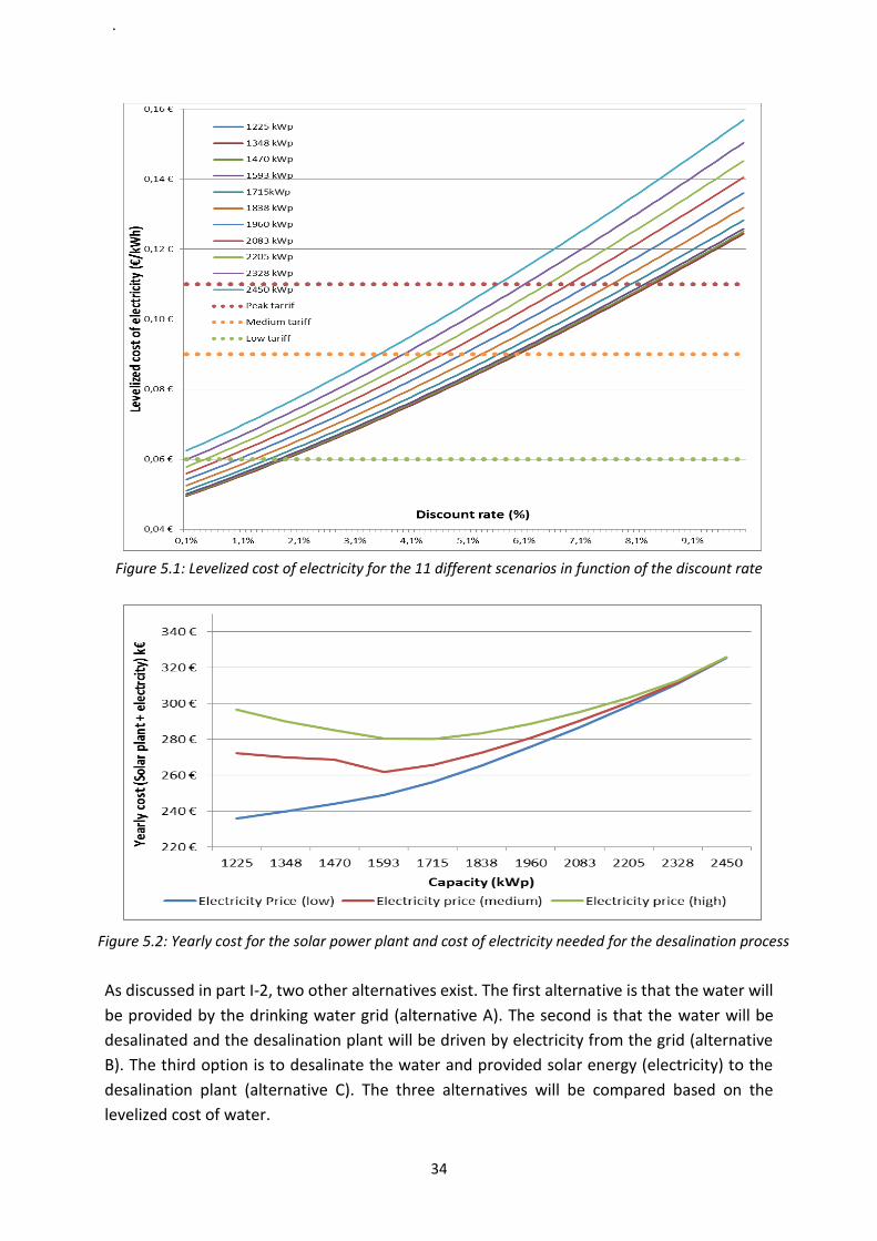
Figure 5.1 and 5.2 represent the levelized cost of electricity in function of the discount rate

and the yearly cost for the 11 different scenarios respectively.

1 Sunshot report. 2012 2 www.oanda.com

.

34

As discussed in part I-2, two other alternatives exist. The first alternative is that the water will

be provided by the drinking water grid (alternative A). The second is that the water will be

desalinated and the desalination plant will be driven by electricity from the grid (alternative

B). The third option is to desalinate the water and provided solar energy (electricity) to the

desalination plant (alternative C). The three alternatives will be compared based on the

levelized cost of water.

Figure 5.1: Levelized cost of electricity for the 11 different scenarios in function of the discount rate

Figure 5.2: Yearly cost for the solar power plant and cost of electricity needed for the desalination process

.

35

As mentioned in the introduction, the desalination plant will produce 1.08Mm3 of fresh water.

Referring to figure 5.2, the yearly cost is assumed to be between 260 000 and 280 000 €. So

the every cubic meter of fresh water produced cost around 0.24 – 0.26 €/m3. This represents

only the supply of energy to the desalination process. In part I-2, it is said that 45% of the

levelized cost of water for the alternative B is due to electricity. In other words, 65% is due to

the desalination plant itself. Table 5.1 summarizes the levelized cost of water for the three

different alternatives.

Alternative Levelized cost of water (€/m3)

A: use of drinking water 0.733 B: desalination plant driven by electric grid 0.737 C: desalination plant driven by solar power 0.72 – 0.74

On an economical point of view, according to table 5.1, it is difficult to give a clear statement

if the desalination plant driven by solar power is beneficial. Some uncertainties on data could

turn the project from profitable to non-profitable. Such data are mainly the discount rate,

transportation costs and civil work. Moreover, the capital cost for the alternative C is much

greater than the other alternatives which make the photovoltaic alternative less attractive.

However some argues that the price of photovoltaic module will continue to decrease but

maybe not as much as some other could guess [41]1 while the efficiency will keep on increasing

[42]2. For this reasons, I would reconsider an economical study of the project in few years.

However, looking at the energy mix for morocco concerning electricity [43]3, 51% of the

electricity come from coal, 20% from oil and 13% from natural gas. Depending on the size of

the potential photovoltaic power plant and the knowing that a conventional coal power plant

emits 1020 kg of CO2 per GWh, a conventional oil power plant emits around 760 kg of CO2

per GWh and a conventional natural gas power plant emits around 515 kg of CO2 per GWh

[44]4, the photovoltaic power plant could save between 1530 tons and 2430 tons of CO2 per

year.

1 M Bazilian. 2013 2 T.M Razykov. 2011 3 Energy mix for Morocco. Source IEA Energy Statistics 4 Conventional CO2 emission for different resources

Table 5.1: Levelized cost of water for the three different alternatives

.

36

References

[1] Observatoire Méditerranéen de l’Energie (OME). Water desalination and solar in the

Mediterranean Region, H. Ben Jallet Allal.. Available at website:

http://www.google.se/url?sa=t&rct=j&q=&esrc=s&source=web&cd=1&ved=0CC0QFjAA&url=http%3

A%2F%2Fwww.cidob.org%2Fes%2Fcontent%2Fdownload%2F24705%2F304888%2Ffile%2FHOUDA%2

BBEN%2BJANNET.pdf&ei=A9KdUa2fMcOm4gTV24DwBQ&usg=AFQjCNFpWSmq01Xyk05MFPnLSlmM

MFPnLS&sig2=GrfKUkZdt0Rv950waljrjg&bvm=bv.46865395,d.bGE Accessed 20/04/2013

[2] Mikael Höök, XuTang; 2012. Depletion of fossil fuels and anthropogenic climate change — a

review. Energy Policy, Volume 52, January 2013, Pages 797-809

[3] Smakhtin, Revenga, Döll; 2004. A pilot global assessment of environmental water requirements

and scarcity. Water International, 2004 - Taylor & Francis

[4] Creativhandz solar solutions. World map of the solar irradiation, source Meteonorm.com.

Available at website: http://www.creativhandz.co.za/solar.php Accessed 24/01/2013

[5] SunShot, Vision and Study, Chapter 4: Photovoltaics: Technologies, cost and performance.

February 2012. Document available at:

http://www.google.se/url?sa=t&rct=j&q=&esrc=s&source=web&cd=1&ved=0CDIQFjAA&url=http%3

A%2F%2Fwww1.eere.energy.gov%2Fsolar%2Fpdfs%2F47927_chapter4.pdf&ei=-NKdUcGhG-

Wj4gSjhYCoDA&usg=AFQjCNGOX5GoG6x9MGTUtfBFTjksqReoxg&sig2=cbm1ycl7RXc3ecLU8G8A4w&

bvm=bv.46865395,d.bGE Accessed 20/04/2013

[6] Baltasar Peñate et al; 2012. Current trends and future prospects in the design of seawater reverse

osmosis desalination technology. Desalination. Volume 284, 4 January 2012, Pages 1–8

[7] A. Soric et al, 2012, Eausmose project desalination by reverse osmosis and battery less solar

energy: Design for a 1m3 per day delivery. Desalination. Volume 301, 3 September 2012, Pages 67–74

[8] Masen webpage, Available at website: http://www.masen.org.ma/index.php?Id=42&lang=fr#/

Accessed 14/04/2012

[9] Google map. Map of the golf course, Available at website:

https://maps.google.com/maps/ms?vps=2&ie=UTF8&hl=fr&oe=UTF8&msa=0&msid=212845077708

205154479.0004baaa5e335bcb0c1d0

[10] National Office for Water in Morocco. Webpage, Available at website: http://www.onep.ma/

Accessed 12/04/2012

[11] National office for Electricity in Morocco. Webpage, Available at website:

http://www.one.org.ma/ Accessed 12/04/2012

.

37

[12] Solargis. Solar irradiation map, Available at website: http://solargis.info/imaps/ Accessed

27/09/2012

[13] Photovoltaics for Professionals: Solar Electric Systems Marketing, Design and Installation; Falk

Antony, Christian Dürschner, Karl-Heinz Remmers; Solarpraxis AG, 2007. P.56

[14] Pvsyst. Webpage of the software, Available at website: http://www.pvsyst.com/en/ Accessed

11/04/2012

[15] Photovoltaics for Professionals: Solar Electric Systems Marketing, Design and Installation; Falk

Antony, Christian Dürschner, Karl-Heinz Remmers; Solarpraxis AG, 2007. P.78

[16] Leonadro seminars (Accessed may 2012) , Available at website:

Seminar 2, Construction and Start Up: http://www.leonardo-energy.org/training-

photovoltaic-systems-session-2-construction-and-start#.UWmTtsr_o0g

Seminar 3, Plant Operation: http://www.leonardo-energy.org/training-photovoltaic-

systems-session-3-plant-operation#.UWmT68r_o0g

Seminar 4, Maintenance: http://www.leonardo-energy.org/training-photovoltaic-

systems-session-4-maintenance#.UWmT_cr_o0g

Seminar 5, Economic Analysis:http://www.leonardo-energy.org/training-photovoltaic-

systems-session-5-economic-analysis#.UWmTfcr_o0g

[17] Oregon University. Sun path diagram generator from Oregon University, Available at website:

http://solardat.uoregon.edu/SunChartProgram.html Accessed 27/04/2012

[18] S. Chen et Al, 2012. Determining the optimum grid-connected photovoltaic inverter size. Elsevier

Solar Energy 87 (2013) 96–116

[19] Applied photovoltaics; S. R. Wenham; Earthscan, 2007. P.77

[20] Photovoltaics for Professionals: Solar Electric Systems Marketing, Design and Installation; Falk

Antony, Christian Dürschner, Karl-Heinz Remmers; Solarpraxis AG, 2007. P.129

[21] Electropaedia. Typical daily electric energy usage profile, Available at website:

http://www.mpoweruk.com/electricity_demand.htm Accessed 12/07/2012

[22] IEA ETSAP Energy Technology System Analysis Programme. Coal-Fired Power, 2010. Document

available at:

http://www.google.se/url?sa=t&rct=j&q=&esrc=s&source=web&cd=1&ved=0CC0QFjAA&url=http%3

A%2F%2Fwww.iea-etsap.org%2Fweb%2FE-TechDS%2FPDF%2FE01-coal-fired-power-GS-AD-

gct.pdf&ei=Q9SdUaGYCKiB4gT77YGQAg&usg=AFQjCNGYdD0cBKfo8NtCtzVIPOPyEq_flw&sig2=mpBKi

4BB9VjeFgQLdkHw9A&bvm=bv.46865395,d.bGE Accessed 22/03/2013

[23] PVtech. Top 10 PV supplier in 2012, Available at website:

http://www.pvtech.org/guest_blog/top_10_pv_module_suppliers_in_2012 Accessed 07/03/2013

.

38

[24] PV insights. Price for solar modules and inverters. PV insights webpage, Available at website:

http://pvinsights.com/index.php Accessed 14/09/2012

[25] Solarbuzz. Price for solar modules and inverters, Available at website: www.solarbuzz.com

Accessed 17/05/2012

[26] Suntech Power. Photovoltaic panel and technical data, Available at website:

http://www.suntech-power.com/en/products/products Accessed 30/05/2012

[27] PV store Europe. Price for PV module, Available at website: http://pvstore-

europe.com/modules-21/suntech Accessed 08/03/2013

[28] Delta solar inverter. Inverter technical data, Available at website: http://www.solar-

inverter.com/eu/en/SOLIVIA_CM_100.htm Accessed 30/05/2012

[29] Photovoltaics for Professionals: Solar Electric Systems Marketing, Design and Installation; Falk

Antony, Christian Dürschner, Karl-Heinz Remmers; Solarpraxis AG, 2007. P.94

[30] PV power. Price for inverter, Available at website: http://www.pvpower.com/commercial-

inverters.aspx Accessed 06/06/2012

[31] Pro solar. Price for support, Available at website: http://www.prosolar.com/prosolar-

new/pages/solarwedge-main2.htm Accessed 07/06/2012

[32] General Electric Energy. Price and technical data for the meter, Available at website:

http://store.gedigitalenergy.com/viewprod.asp?Model=PQMII Accessed 06/06/2012

[33] V.M Fthenakis et al, 2010. Photovoltaics: Life-cycle analyses. Elsevier. Solar Energy 85 (2011)

1609–1628

[34] A. Stoppato, 2008. Life cycle assessment of photovoltaic electricity generation. Elsevier. Energy

33 (2008) 224–232

[35] Same as source [16]

[36] TE connectivity. Price for the combiner box, Available at website:

http://se.mouser.com/ProductDetail/TE-Connectivity/1954283-

1/?qs=XhI5AayaxxVkdty4g1HGmA%3d%3d Accessed 07/06/2012

[37] D. Zejli et al, 2004. Economic analysis of wind-powered desalination in the south of Morocco. Elsevier. Desalination 165 (2004) 219-230

[38] G. Notton et al, 1998. Costing of a stand-alone photovoltaic system. Elsevier. Energy Vol. 23, No.

4, pp. 289–308, 1998

.

39

[39] SunShot. D Feldman et al. Photovaltaic pricing trends: Historical, recent and near-term

projections. November 2012 Report available at:

http://www.google.se/url?sa=t&rct=j&q=&esrc=s&source=web&cd=1&ved=0CDAQFjAA&url=http%3

A%2F%2Fwww.nrel.gov%2Fdocs%2Ffy13osti%2F56776.pdf&ei=p9SdUafUDfT04QSdqoDIBQ&usg=AF

QjCNHCkBSRrGUFH7oklTUU2yu6yL8X4Q&sig2=iWOG76HEnWsePBgLbJrWfw&bvm=bv.46865395,d.b

GE Accessed 20/03/2013

[40] Oanda. Exchange rate in 2011, Available at website:

http://www.oanda.com/lang/fr/currency/historical-rates/ Accessed 17/04/2013

[41] M. Bazilian et al, 2013. Re-considering the Economics of Photovoltaic Power. Elsevier.

Renewable Energy Volume 53, May 2013, Pages 329–338

[42] T.M. Razykov, 2011. Solar photovoltaic electricity: Current status and future prospects. Elsvier.

Solar Energy Volume 85, Issue 8, August 2011, Pages 1580–1608 Progress in Solar Energy 1

[43] IEA statistics. Morocco energy mix for the electricity usage from IEA Energy Statistics, Available

at website: http://www.iea.org/stats/electricitydata.asp?COUNTRY_CODE=MA Accessed 23/05/2013

[44] Environmental Protection Agency. Conventional CO2 emission for different resources, Available

at website: http://www.epa.gov/cleanenergy/energy-and-you/affect/air-emissions.html Accessed

23/05/2013

.

40

Appendix

Watering of the golf course “Golf des Dunes” in Agadir, Morocco.

Part 1: The desalination plant.

The document mentioned in the introduction and which is the precursor of this thesis has been written

by Mehdi Berrada and Simon Caron. However as the document is written in French, a short summary

of it is developed in this appendix.

The aim of the document was to conduct a techno-economic feasibility analysis of a desalination plant

supplying the fresh water demand of a golf course in Agadir, Morocco.

In the first part, the document explains the context of the research which is similar to the “context”

part of this thesis.

Secondly, it explains in depth the functioning of a reverse osmosis desalination plant, its different

components and how much fresh water will be produced.

Finally it gives a detailed economic analysis of the desalination plant, including its electricity usage.