accelerometer and magnetometer based gyroscope … · destinée au dépôt et à la diffusion de...

HAL Id: hal-00826243https://hal-upec-upem.archives-ouvertes.fr/hal-00826243

Submitted on 27 May 2013

HAL is a multi-disciplinary open accessarchive for the deposit and dissemination of sci-entific research documents, whether they are pub-lished or not. The documents may come fromteaching and research institutions in France orabroad, or from public or private research centers.

L’archive ouverte pluridisciplinaire HAL, estdestinée au dépôt et à la diffusion de documentsscientifiques de niveau recherche, publiés ou non,émanant des établissements d’enseignement et derecherche français ou étrangers, des laboratoirespublics ou privés.

Accelerometer and Magnetometer Based GyroscopeEmulation on Smart Sensor for a Virtual Reality

ApplicationBaptiste Delporte, Laurent Perroton, Thierry Grandpierre, Jacques Trichet

To cite this version:Baptiste Delporte, Laurent Perroton, Thierry Grandpierre, Jacques Trichet. Accelerometer and Mag-netometer Based Gyroscope Emulation on Smart Sensor for a Virtual Reality Application. Sensorand Transducers Journal, 2012, 14-1 (Special Issue ISSN 1726-5479), p32-p47. <hal-00826243>

https://hal-upec-upem.archives-ouvertes.fr/hal-00826243

https://hal.archives-ouvertes.fr

Sensors & Transducers Journal, Vol.0,Issue 0, Month 2011,pp.

Accelerometer and Magnetometer Based Gyroscope Emulation

on Smart Sensor for a Virtual Reality Application

Baptiste Delporte, Laurent Perroton, Thierry Grandpierre

and Jacques Trichet1

Université Paris Est, ESIEE Engineering, Marne-la-vallée, France 1Freescale Semiconductor, Inc. Toulouse, France

Received: /Accepted: /Published:

Abstract: In this paper, we propose two methods based on quaternions to compute the angles of

inclination and the angular velocity with 6 degrees of freedom using the measurements of a 3-axis

accelerometer and a 3-axis magnetometer. Each method has singularities which occur during the

computation of the orientation of the device in the 3-dimensional space. We propose solutions to avoid

these singularities. Experimental results are given to compare our model with a real gyroscope.

Keywords: smart sensor; sensor fusion; accelerometer; magnetometer; angular velocity; gyroscope

1. Introduction

The computation of the angles of inclination of a device and its angular velocity has many applications

for aeronautics, transportation systems, human motion tracking, games and virtual reality. Classical

methods use accelerometers, magnetometers and gyroscopes. For some particular angles, there are

singularities for which it is impossible to compute neither the orientation of the device in the 3-

dimensional space nor its angular velocity [8, page 407].

Our goal is to design a smart sensor magnetometer based virtual gyroscope, i.e. a method to compute

the angular velocity based on the measurements of a 3-axis accelerometer and a 3-axis magnetometer,

without any gyroscope, and with 6 degrees of freedom: 3 degrees of freedom are provided by the


accelerometer and the others are provided by the magnetometer. It is easier to implement, less

expensive and has lower power consumption than the classical gyroscope solutions. Our target is small

motion tracking with embedded devices like cellular phones, with application fields like virtual or

augmented reality. Moreover, it is possible to create a virtual gyroscope with a magnetometer and an

accelerometer, whereas it is not possible to create a virtual magnetometer or a virtual accelerometer

using only a gyroscope. Methods with accelerometers only have been already proposed in [2, 3, 6, 7].

A well-known method to compute a strap down gyroscope output simply consists in differentiating the

angles of inclination of the device, but we want to compute the total angular velocity, which is the

addition of the angular velocities about the three axes of the fixed frame.

Two methods with two different approaches have been developed. They are proposed in this paper.

The method that uses the angles of inclination of the device has been implemented. The method that

uses the rotation matrix will be implemented and the two methods will be compared in order to find

the method which offers the best precision on the target architecture. This work is a collaboration

project between Freescale and ESIEE Engineering School which started in June 2010.

In Section 2, we introduce the platform and the sensors. In Section 3, a first method to compute the

angular velocity using the absolute angles of inclination is presented. In Section 4, a second method to

compute the angular velocity using the rotation matrix is presented. In Section 5, experimental results

are given and a virtual reality application is presented.

2. Hardware and Smart Sensors

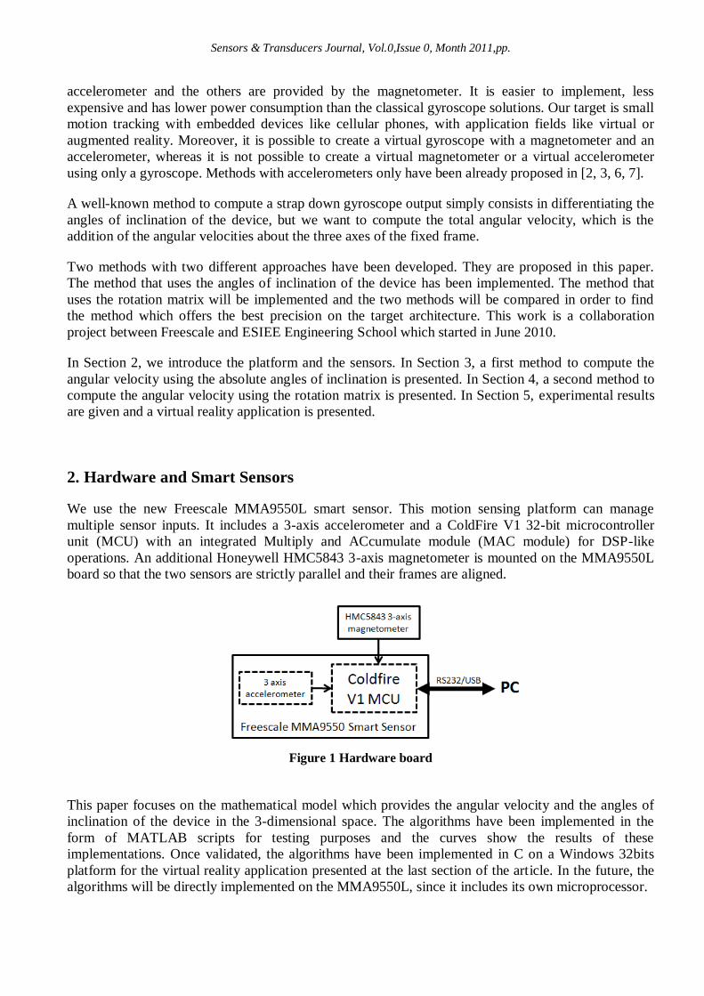
We use the new Freescale MMA9550L smart sensor. This motion sensing platform can manage

multiple sensor inputs. It includes a 3-axis accelerometer and a ColdFire V1 32-bit microcontroller

unit (MCU) with an integrated Multiply and ACcumulate module (MAC module) for DSP-like

operations. An additional Honeywell HMC5843 3-axis magnetometer is mounted on the MMA9550L

board so that the two sensors are strictly parallel and their frames are aligned.

Figure 1 Hardware board

This paper focuses on the mathematical model which provides the angular velocity and the angles of

inclination of the device in the 3-dimensional space. The algorithms have been implemented in the

form of MATLAB scripts for testing purposes and the curves show the results of these

implementations. Once validated, the algorithms have been implemented in C on a Windows 32bits

platform for the virtual reality application presented at the last section of the article. In the future, the

algorithms will be directly implemented on the MMA9550L, since it includes its own microprocessor.


3. Virtual Gyroscope Based on the Angles of Inclination of the Device

In this section, the angles of inclination and the angular velocity are computed from the accelerometer

and the magnetometer measurements using Tait-Bryan angles and quaternions.

3.1 Parameterization of Rotations with Tait-Bryan Angles

In order to describe the orientation of the device in the 3-dimensional space, 2 right-handed Cartesian

coordinate systems are used: a fixed reference frame with North, East and Down (NED

convention), and denoted by the subscript , and a moving frame attached to a mobile device, denoted

by the subscript . The reference frame and the device frame are aligned when the device is flat and

aligned with the axis pointed to magnetic North. Rotation angles are positive when clockwise

viewed along the relevant axis vector in the positive direction.

The orientation of the device in the reference frame can be described by Tait-Bryan angles: , and

. is the angle of rotation about the axis (yaw). is the angle of rotation about the axis (pitch).

is the angle of rotation about the axis (roll). Any rotation of the device can be expressed as a

composition of these three rotations in the reference frame, as shown in Fig. 2.

Figure 2. Tait-Briant angles.

A rotation about the axis, the axis or the axis can be respectively described by a rotation

matrix , or :


The composition of the 3 rotations about the axis, then the axis and finally the axis, is

described by the rotation matrix .

It is possible to compute , , and the angular velocity from the Earth’s magnetic field ,

expressed in the device frame, and the Earth’s gravitational field , expressed in the device frame.

The magnetic field is measured by the magnetometer. On the other hand, the accelerometer measures

the total acceleration including the gravitational field, the acceleration provided by the user and the

acceleration due to the Coriolis force. Consequently, an extraction of the gravitational field needs

to be performed with a filter.

The expression of the Earth’s magnetic field in the reference frame is given by

where denotes the strength of the magnetic field (in Teslas),

denotes the angle of inclination of the magnetic field, which depends on the location on the Earth, and

denotes the transpose of .

The expression of the Earth’s gravitational field in the reference frame is given by

where denotes the strength of the gravitational field, i.e. the acceleration (in Newtons).

The computation process is shown in Fig. 3.

Figure 3. Computation process 1

3.2 Extraction of

Since is a constant offset in the measurement of , it can be extracted with a low-pass filter. The

resulting vector contains sensor medium frequencies and spurious noise. In order to keep only , a

sliding median filter and a sliding average filter are used, as shown in Fig. 4. The same delay is applied

to to make sure they are in phase.

Figure 4. Computation of

3.2.1 Low-Pass Filter

The frequency of equals 0. Consequently, the gravitational field can be extracted with a first-order

Butterworth low-pass filter. The Z-transform transfer function of the filter is given by:


The default coefficients have been computed with MATLAB by synthesizing a low-pass filter with an

experimentally determined cut-off frequency , where denotes the sampling frequency.

They are given by . If a variation of the norm exceeds a

threshold, the cut-off frequency of the Butterworth filter increases of and the coefficients

are computed again. If the cut-off frequency reaches , the filter waits for the

norm to stabilize. Then, decreases of until it reaches . Then, is kept, until

the norm exceeds again the threshold. A threshold of has been experimentally

determined.

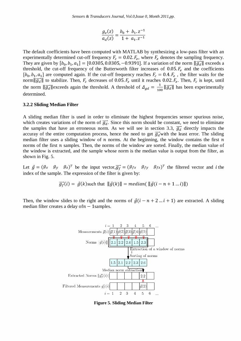
3.2.2 Sliding Median Filter

A sliding median filter is used in order to eliminate the highest frequencies sensor spurious noise,

which creates variations of the norm of . Since this norm should be constant, we need to eliminate

the samples that have an erroneous norm. As we will see in section 3.3, directly impacts the

accuray of the entire computation process, hence the need to get with the least error. The sliding

median filter uses a sliding window of norms. At the beginning, the window contains the first

norms of the first samples. Then, the norms of the window are sorted. Finally, the median value of

the window is extracted, and the sample whose norm is the median value is output from the filter, as

shown in Fig. 5.

Let be the input vector, the filtered vector and the

index of the sample. The expression of the filter is given by:

Then, the window slides to the right and the norms of are extracted. A sliding

median filter creates a delay of samples.

Figure 5. Sliding Median Filter


The gravitational field filtered with the sliding median filter still has variations, a sliding

average filter is used to smooth it.

3.2.3 Sliding Average Filter

The sliding average filter uses a sliding window of n samples. At the beginning, the window

contains the first samples. Then, the average value of the window is extracted and output

from the filter.

Let be the input vector, the filtered vector and

the index of the sample. The expression of the filter is given by:

Then, the window slides to the right and filters the values . A sliding

average filter creates a delay of samples.

3.3 Computation of the Angles of Inclination

The Earth’s magnetic field , expressed in the device frame, results from the rotation of the

magnetic field , expressed in the reference frame.

(1)

The Earth’s gravitational field , , expressed in the device frame, results from the rotation of

the gravitational field , expressed in the reference frame. Since remains unchanged after

a rotation about the axis, . It follows:

(2)

It is possible to compute the roll angle from the gravitational field by developing Eq. 2:

(3)

arctan2 denotes the arctangent on the domain – .

Once is known, it is possible to compute :

(4)

arctan denotes the arctangent on the domain – .

If is aligned with the axis, the denominator in Eq. 4 becomes 0. Please see Tab. 1 for


the detection of this singularity.

Once and are known, it is possible to compute by developing Eq. 1:

3.4 Singularity Detection

A table of the singularities is given in Tab. 1. The normalized gravitational and magnetic field

in the device frame are denoted respectively by and

. If a singularity is detected, several compositions of

rotations give the same result. Consequently, there are two methods. The first method consists

in keeping the previous values of , and . The second method consists in finding the

appropriate case that allows the accurate determination of , and .

1 0 sin(δ) cos(δ)

0

0

1 0 sin(δ) -cos(δ) 0

0

0 -1 cos(δ) -sin(δ)

0

0

0 -1 -cos(δ) -sin(δ)

0

0

-1 0 -sin(δ) -cos(δ)

0

0

-1 0 -sin(δ) -cos(δ) 0

0

0 -1 -cos(δ) sin(δ)

0

0

0 -1 cos(δ) sin(δ)

0

0

Table 1. Table of Singularities


3.5 Parameterization of Rotations with Quaternions

The quaternions are hypercomplex numbers, i.e. 4-dimensional mathematical objects, used to

describe rotations in the 3-dimensional space [5].

3.5.1 Definition and Properties of a Quaternion

A quaternion has 4 coordinates in a 4-dimensional vector space and is denoted by

with . It consists of a vector part

and a scalar part . It can be expressed in the following form:

(5)

In Eq. 5, , and are imaginary numbers: , and ,

, . Therefore, it is possible to compute the product of two

quaternions and , denoted by ,

using the properties of the hypercomplex numbers. It can be noticed that the product between

2 quaternions is not commutative: .

The inverse of a quaternion is denoted by

.

3.5.2 Euler-Rodrigues Parameters

A quaternion can be used to describe a rotation by an angle about

a unit vector that is the axis. is a unit vector, so . The Euler-

Rodrigues parameters corresponding to the rotation are given by:

3.5.3 Rotation

Let be a vector. The quaternion transforms into another vector

by rotating it by angle about an axis. A fourth null coordinate is added to

, so it becomes . The rotated vector corresponds to the vector part

of given by:

(6)

The scalar part of is 0, since is a pure vector in the 3-dimensional space.


3.5.4 Composition of Two Rotations

Let be a quaternion describing a rotation by an angle about an axis and a

quaternion describing a rotation by an angle about an axis . The composition of the

rotations about the axis, then the axis, is given by the quaternion . Let

be a vector. The quaternion transforms into another vector

by rotating it by angle about an axis , then by angle about an axis .

With , the expression of Eq. 6 becomes

. The rotated vector corresponds to the vector part of . The scalar part of

is 0, since is a pure vector in the 3-dimensional space.

3.5.5 Computation of the Angular Velocity

The instantaneous angular velocity of the device at the instant , expressed in the

reference frame, corresponds to the vector part of given by [4]:

The scalar part of is 0, since is a pure vector in the 3-dimensional space, which

finally gives:

3.6 Computation of the Quaternion From the Angles of Inclination

A rotation by angle about the axis, by angle about the axis or by angle about the

axis can be respectively described by the quaternion ,

, or . The quaternion

describing the composition of the rotations about the axis, then the axis, and finally the

axis, is given by .

The method described above has 8 singularities. Consequently, the computation of the angles

, and cannot be accurate if the detection of singularities is not efficient enough.

4 Virtual Gyroscope Based on the Rotation Matrix

In this section, the angles of inclination of the device and the angular velocity are computed

from the accelerometer and the magnetometer measurements using the rotation matrix and


quaternions. Although its computation cost is higher, the major advantage of this method is

that it reduces the number of singularities to only 2. Furthermore, this method does not require

the explicit computation of the angles. The computation process is shown in Fig. 6.

Figure 6. Computation Process 2

4.1 Computation of the Rotation Matrix

Let be a vector. The rotation matrix transforms into another vector

by rotating it by an unknown angle about an unknown axis . The

coordinates of the resulting are given by:

(7)

Once and are known, it is possible to compute . Consequently, we will be able to

deduce and .

Let be the normalized gravitational field in the device frame, the

normalized magnetic field in the device frame, the cross product between the

gravitational field and the magnetic field in the device frame, ,

and .

On the other hand, let be the normalized gravitational field in the reference frame,

the normalized magnetic field in the reference frame, the cross

product between the gravitational field and the magnetic field in the reference frame,

, and .

The expressions of and are respectively given by and

. Consequently, , ,

and .


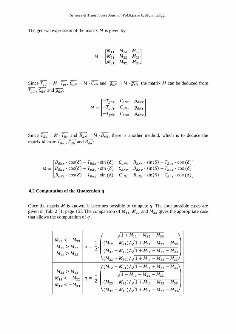
The general expression of the matrix is given by:

Since , and , the matrix can be deduced from

, and :

Since and , there is another method, which is to deduce the

matrix from , and :

4.2 Computation of the Quaternion

Once the matrix is known, it becomes possible to compute . The four possible cases are

given in Tab. 2 [1, page 15]. The comparison of , and gives the appropriate case

that allows the computation of .


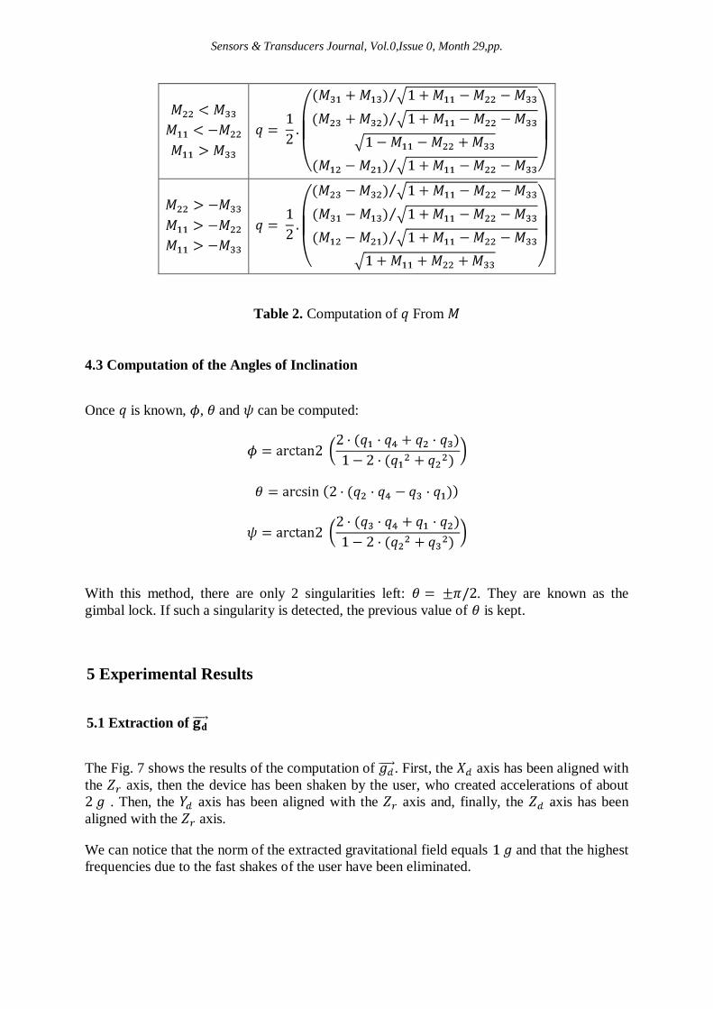
Table 2. Computation of From

4.3 Computation of the Angles of Inclination

Once is known, , and can be computed:

With this method, there are only 2 singularities left: . They are known as the

gimbal lock. If such a singularity is detected, the previous value of is kept.

5 Experimental Results

5.1 Extraction of

The Fig. 7 shows the results of the computation of . First, the axis has been aligned with

the axis, then the device has been shaken by the user, who created accelerations of about

. Then, the axis has been aligned with the axis and, finally, the axis has been

aligned with the axis.

We can notice that the norm of the extracted gravitational field equals and that the highest

frequencies due to the fast shakes of the user have been eliminated.


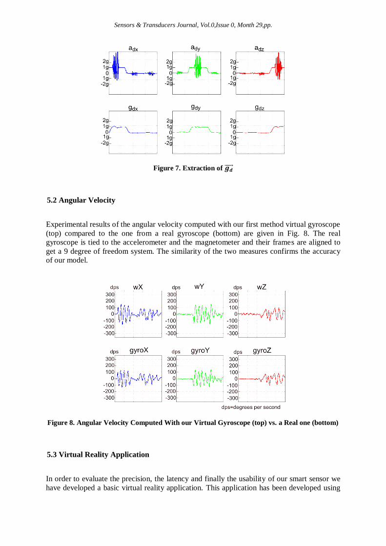
Figure 7. Extraction of

5.2 Angular Velocity

Experimental results of the angular velocity computed with our first method virtual gyroscope

(top) compared to the one from a real gyroscope (bottom) are given in Fig. 8. The real

gyroscope is tied to the accelerometer and the magnetometer and their frames are aligned to

get a 9 degree of freedom system. The similarity of the two measures confirms the accuracy

of our model.

Figure 8. Angular Velocity Computed With our Virtual Gyroscope (top) vs. a Real one (bottom)

5.3 Virtual Reality Application

In order to evaluate the precision, the latency and finally the usability of our smart sensor we

have developed a basic virtual reality application. This application has been developed using


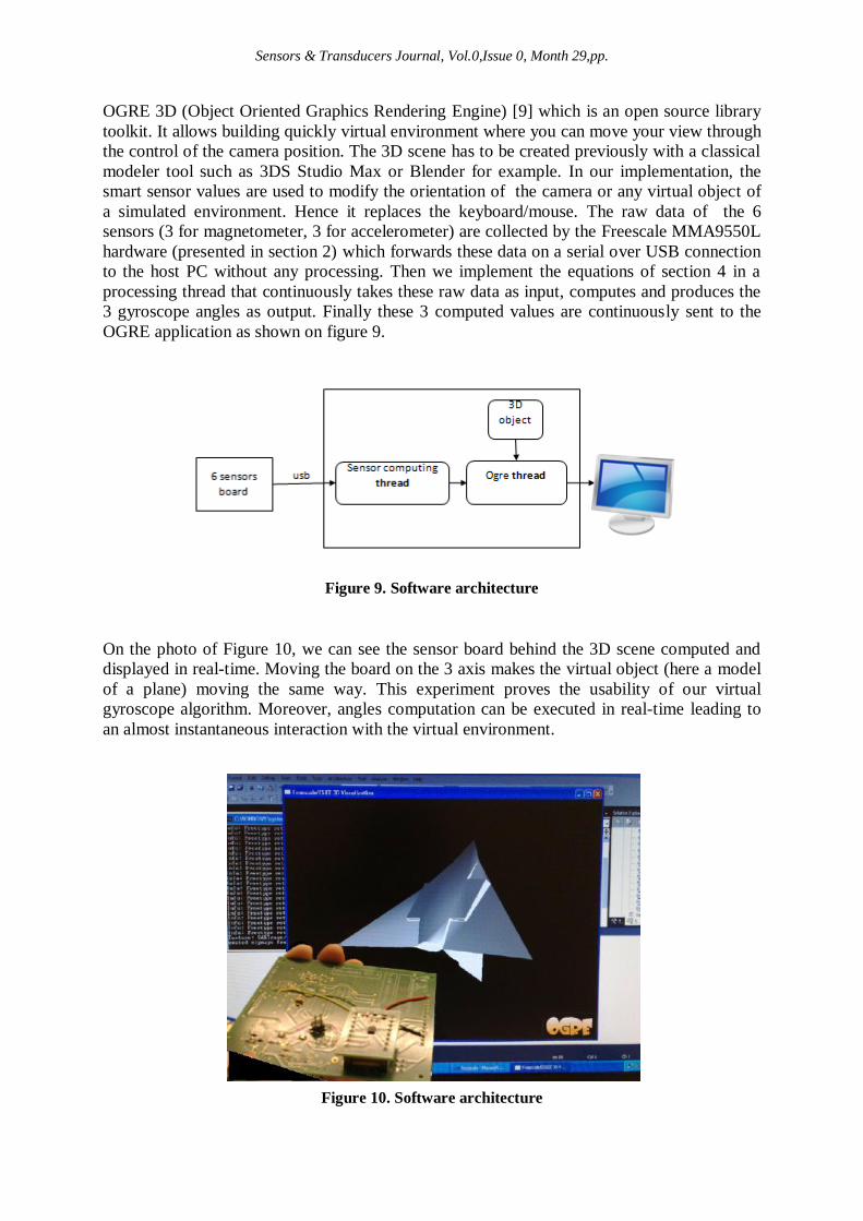
OGRE 3D (Object Oriented Graphics Rendering Engine) [9] which is an open source library

toolkit. It allows building quickly virtual environment where you can move your view through

the control of the camera position. The 3D scene has to be created previously with a classical

modeler tool such as 3DS Studio Max or Blender for example. In our implementation, the

smart sensor values are used to modify the orientation of the camera or any virtual object of

a simulated environment. Hence it replaces the keyboard/mouse. The raw data of the 6

sensors (3 for magnetometer, 3 for accelerometer) are collected by the Freescale MMA9550L

hardware (presented in section 2) which forwards these data on a serial over USB connection

to the host PC without any processing. Then we implement the equations of section 4 in a

processing thread that continuously takes these raw data as input, computes and produces the

3 gyroscope angles as output. Finally these 3 computed values are continuously sent to the

OGRE application as shown on figure 9.

Figure 9. Software architecture

On the photo of Figure 10, we can see the sensor board behind the 3D scene computed and

displayed in real-time. Moving the board on the 3 axis makes the virtual object (here a model

of a plane) moving the same way. This experiment proves the usability of our virtual

gyroscope algorithm. Moreover, angles computation can be executed in real-time leading to

an almost instantaneous interaction with the virtual environment.

Figure 10. Software architecture


6 Conclusion and Future Works

In this paper, we have presented two methods to implement a virtual gyroscope that only uses

the measurements of an accelerometer and a magnetometer, with 6 degrees of freedom.

The two methods have their own advantages and drawbacks. The method which uses the

angles of inclination is easier to implement, but there are 8 singularities, which need to be

solved. Moreover, the computation of depends on the computation of θ, which in turns

depends on . If there is a singularity on , the computation of the angles is not possible. On

the other hand, the method with the rotation matrix has only two singularities but its

computation cost is higher. The second method has not been completely implemented and

validated yet; this is our current work.

The precision of both methods and their limitations must be investigated and will be our main

future work.

Finally, we plan to optimize the implementation of both methods on the MMA9550L. This

will allow us to provide the angular velocity and the angles of inclination of the device and

use them for several applications, like a 3-dimensional mouse, a virtual joystick, a human

motion tracker. The MMA9550L board can communicate with the PC with a Bluetooth

connection. Consequently, the board can become a portable device with its own power

supply.

Acknowledgment

The authors would like to thank Freescale for their support, the platform, and Mr. Mark

Pedley whose work is the base of this project.

References

[1] J. Diebel. Representing attitude: Euler angles, unit quaternions, and rotation vectors.

Technical report, Stanford University, California 94301-9010, october 2006.

[2] T. Liu, G.-R. Zhao, and S. Pan. New calculating method of angular velocity in

gyroscope-free strapdown inertial navigation systems. Systems Engineering and

Electronics, 32(1):162–165, January 2010.

[3] P. Schopp, L. Klingbeil, C. Peters, A. Buhmann, and Y. Manoli. Sensor fusion

algorithm and calibration for a gyroscope-free imu. In Proceedings of the Eurosensors

23rd Conference, volume 1, pages 1323–1326, 2009.

[4] A. L. Schwab. Quaternions, finite rotation and Euler parameters, 2002.

[5] D. Stahlke. Quaternions in classical mechanics, 2007.


[6] C. Wang, J.-X. Dong, S.-H. Y., and X.-W. Kong. Hybrid algorithm for angular

velocity calculation in a gyroscope-free strapdown inertial navigation system. Journal of

Chinese Inertial Technology, 18(4):401–404, 2010.

[7] X.-N. Wang, S.-Z. Wang, and H.-B. Zhu. Study on models of gyroscope-free strap-

down inertial navigation system. Binggong Xuebao/Acta Armamentarii, 27(2):288–292,

2006.

[8] J. R. Wertz. Spacecraft Attitude Determination and Control. D. Reidel Publishing

Company, Dordrecht, Holland, 1978.

[9] http://www.ogre3d.org

accelerometer and magnetometer based gyroscope … · destinée au dépôt et à la diffusion de...

Documents