abstract - national university of...

Abstract

Abstract

The basis of this multi-disciplinary project is to reverse engineer, integrate, automate

and flight-test an unmanned miniature Flying Wing Air vehicle. This project was

done in close collaboration with industrial aircraft manufacturers, Cradence Services ,

principally centered about their latest miniature drone, the Golden Eagle, together

with my colleague Mr. Low Jun Horng whose efforts were mainly in integration,

flight controls and automating the craft for GPS waypoint flight.

This study establishes a reverse engineering routine primarily for the aerodynamic

data generation for an unconventional miniature reflexed Flying Wing airfoil, for

which there was insufficient contractors’ aerodynamic data and stability derivatives

provided. The thesis then goes on to describe in detail also a material research and

selection procedures and the reverse-prototyping of the test platforms for which there

was also insufficient contactors specification. With these accomplished, we then

focused on further analysis and modification to the original power plant to enable the

platform to carry an additional payload of 250g, which encompasses an autonomous

navigation system, and a real time operating camera. Some of the techniques adopted

were 3D Laser profile scanning, Computational Fluid Dynamics studies, weight and

balance matching, CG and Inertia tensor estimation and a series of coordinated glide

and flight tests. Various tests were done through the course of the project to validate

and proof the integrity of theoretical results derived. Results of the calculations were

found to be consistent and useful in characterizing the unknown airfoil.

A paper based on this project was presented at the Republic of Singapore Air Force’s

(RSAF) Aerospace Technology Seminar on February 2005.

National University of Singapore i Department of Mechanical Engineering

Acknowledgements

Acknowledgements

The author would like to extend sincere gratitude to his project supervisor, Associate

Professor Gerard Leng Siew Bing for his guidance, and above all patience in

answering all queries pertaining to the project. Also, the authors would like to thank

Mr Leong See Kit of Cradence Pte Ltd for allowing us to use his equipment during

the course of this project.

Special thanks, also to Mr Low Jun Horng, Student, FYP AM23, for his hard work

and dedication in getting the prototypes working and for integration of the control

system.

The author will also like to extend his gratitude to the staff of Dynamics Laboratory,

Encik Ahmad Bin Kasa, Ms Amy Chee, Ms Priscilla Lee, and Mr Cheng Kok Seng,

for their assistance for the duration of the project, and as well as Mr Neo Ken Soon of

the Advanced Manufacturing Laboratory for his assistance in the use of the 3D Laser.

National University of Singapore ii Department of Mechanical Engineering

Table of Contents

Table of Contents

Abstract................................................................................................................I

Acknowledgement……………………………………………………….….….II

List of Figures……………………………………………………………..…..VII

List of Tables………………………………………………………………..…VIII

List of Symbols……………………………………………………………..… X

List of Subscripts…………………………………………………………..…..XII

Chapter 1: Introduction

1.1 Thesis Background………….......................................................................1

1.2 Objectives …………………………………………………………….……3

1.3 The Golden Eagle Micro Air Vehicle (MAV)………………………….….4

1.4 Goals to Achieve……………………………………………………….…..6

1.5 Structure of Dissertation…………………………………………………...7

Chapter 2: Literature Survey 2.1 History of Flying Wing Concept & Applications …………………………8

2.2 Concept and Theory behind the Flying Wing………………………........9

2.2.1 Swept Wings…………………………………………………....11

2.2.2 Reflexed Wings…………………………………………….…...12

2.2.3 Tailed-Tip Wings……………………………………………….13

2.2.4 Lowered CG…………………………………….……………....13

Chapter 3: Theoretical Analysis of Airfoil Aerodynamics


Table of Contents

3.1 Aerodynamic Forces and Coefficients..……………………………….….15

3.2 Aerodynamic Moments and Pitching Moments…………………………..16

3.2.1 Effect of Camber on Cm……………………………………...…17

3.3 Self Stabilizing Reflexed wings……………….………………………….18

3.4 Coupled Control Surfaces……………………...………………………….21

Chapter 4: Preliminary CFD Analysis

4.1 Rationale behind the need for CFD Analysis……………………….........22

4.2 Airfoil Profiling……..……………………………………………………23

4.2.1 Laser Profile Photography…………………………………..….23

4.2.2 CAD Modeling…………………………………………..……..24

4.3 Performing the Preliminary Analysis……………………………….……25

4.3.1 Preparation of CFD Mesh…………………………….…….….25

4.3.2 Simulation Model…………………............................................26

4.3.3 Relevant Parameters………………............................................28

4.4 Results and Discussion………….………………………………………..29

Chapter 5: Prototype Fabrication

5.1 Reasons for Reverse Prototyping……………………………………....…32

5.1.1 Model Dimensioning……………………………………..….….33

5.2 Material Research and Selection………………………………....…….....33

5.3 Structural Construction………………………………………………....…35

5.3.1 Tissue Fiber Laying…………………………………….…...…. 35

5.3.2 Wing and Fuselage……………………………………………...36

5.4 Assembly………………………………………………………………….36

National University of Singapore iii Department of Mechanical Engineering

Table of Contents

Chapter 6: Estimation of CG and Mass of Inertias

6.1 Aerodynamic Centre and CG Positioning…………………….……….37

6.2 Static Margin…………………………………………………………..40

6.3 Mass of Inertia Estimation...………………………………….………..40

Chapter 7: Experimental Results and Analysis

7.1 Preliminary Glide Test…………………………………………………..43

7.1.1 Glide Test Theory……………………………………………..43

7.1.2 Experimental Set-up and Calibration………………………….43

7.1.3 Test Environment……………………………………………...45

7.1.4 Aero Coefficient Verification………………………………….45

7.2 Discussion………………………………………………………………..45

Chapter 8: Propulsion System Integration

8.1 Propulsion Systems…………………………………………………….....47

8.1.1 Theoretical Analysis…………………………………….……....47

8.1.2 Experimental Set-up………………………………….…….…...48

8.1.3 Analysis of Data……………………………………….………..49

8.2 Discussion………………………………………………………..……….49

Chapter 9: Flight Testing

9.1 Outdoor Windless Testing: Powered …..…………………………..……50

9.1.1 Test Sites……………………………………………….………50

9.1.2 Test Routine……………………………………………….…...50

National University of Singapore iv Department of Mechanical Engineering

Table of Contents

9.1.3 Problems………………………………………………………..51

9.2 Test Data Gathered………………………………………………….……51

9.3 Flight Test Results…………………………………………………..……52

9.4 Discussion…………………………………………………………..….…53

Chapter 10: Conclusion………….………………………………….….….54

Chapter 11: Recommendations………………………………….…….…..56

References:………………………………………..……………….…….…..57

Appendix (A-B):………………………………………………….………….60

Appendix A CFD Results and Aerodynamic Plots………………..……......…..I

Appendix B Typical airfoil Section Characteristics……..………..…….…....VIII

Appendix C: Propulsion Systems Design …………………………..….….......X

Appendix D: Aerofoil Concepts……………………………………..….….....XV

Appendix E: Weight and Balance Matching………………………..…….….XIX

Appendix F: Static Margin Determination…………………………..…….…XXV

Appendix G: Component Weights Breakdown……………………..…...….XXVII

Appendix H: Camber Distribution of Airfoils…………….……..………….XXVIII

Appendix I: Benefits and Disadvantages of Flying Wings//……..……….….XXIX

National University of Singapore v Department of Mechanical Engineering

List of Figures

List of Figures

Figure Description Page No.

1 Modern Flying Wing UAVs in service today

2

2 Shape of the UAV (rear view) 4

3

4

The Golden Eagle

Golden Eagle Dimensional Drawing

4

5

5 Flying Wings: B2, Boing Blended Wing and RB-35 9

6

7

8

Natural Nose down Moments of Conventional Airfoils

Instability of Conventional Airfoils

Sweep Angle on a backward swept wing

10

10

11

9 Twist Angle on a wing section 11

10 Sketch of a Reflexed Airfoil 12

11 Highly swept wing with angled winglets. 13

12 Low CG positioning on the Pelican MAV 14

13 Counter Moments of Reflex Airfoil 14

14 The 4 main forces on the airfoil 15

15 Flight Angle Definition 15

16 The Moments on an airfoil 17

17 Camber Profile Definition 18

18 Golden Eagle’s matching reflex wing profile 18

19

20

21

Elevons indicated by Yellow arrows

3-D Laser scanning and Reverse aerofoil CAD model

CAD drawing of the UAV

21

23

25


List of Figures

22

23

24

25

26

27

28

29

30

31

32

33

34

35

36

37

38

39

40

41

42

43

44

CAD model of the UAV Meshed Model of the Golden Eagle 3D-Control Volume CFD Plot of Pessure Distribution over aircraft Polar Plots of Aerodynamic Coefficients Eleven Sectioned ribs along the Wing Pouring of the resin GFRP right wing bottom shell up Assembled ribs

Assembly Layout

CG Balancing Chart

Location of AC with respect to the CG

Experimental verification of CG position

Geometrical Estimation of Inertias

Glide Slope Angle definition

Glide Test Grounds

Speed Measurement Setup

Pshaft and ηm versus Ωm for a Speed-400 motor Thrust measurement: Test Stand Setup The 9x6 Pusher Propeller Altitude ascend Prototype 3 Testing of Protoype 4 with 6x4 Propeller

25

25

28

29

30

33

35

35

36

36

37

39

39

41

43

43

44

47

48

49

50

53

56


List of Tables

List of Tables

Table Description Page No.

1

2

3

4

5

The Turbulent Flow CFD computation results

Comparison of Fiber properties (Ref: Hull & Clyne)

Comparison of Resin properties (Ref: Hull & Clyne)

Component Weights

Thrust Experimental Results

29

34

34

37

49

National University of Singapore i Department of Mechanical Engineering

List of Symbols

List of Symbols

Symbol Description

Arotor Area of propeller disk / m2

Cd Coefficient of Drag for airfoil

CL Airfoil lift coefficient

CL,max Maximum lift coefficient

c Airfoil Chord / m

CP Coefficient of Power

cp Power coefficient for propeller

cp,total Total Power coefficient of propeller

CT Coefficient of Thrust

cT, prop Thrust coefficient for propeller

cT, Total Power coefficient for propeller

Cm

Cm,c/4

Coefficient of Moments

Airfoil pitching moment about the quarter-chord point

d Diameter /m

D Diameter of Propeller / m

I

Ixx

Iyy

Izz

Iyz

Izx

Current / A

Moment of Inertia about x axis

Moment of Inertia about y axis

Moment of Inertia about z axis

Product of Inertia about y and z axis

Product of Inertia about z and x axis


List of Symbols

Ixy

L

Product of Inertia about the x and y axis

Length / m

M Mass / kg

Mbi Reading of digital balance due to mass / kg

p Total pressure / Pa

P Power / kW

Pinduced Induced power / kW

Ptotal Total power due to Propeller and motor

rprop Radius of Propeller / m

Re Reynold’s number

T Thrust / N

tduct Thickness of duct / m

V Voltage / V

V Velocity at propeller disk / m/s

W Weight of Prototype / kg

α Glide Angle

ρ Density of air, = 1.21 kg/m3 unless stated otherwise

Ω Angular Velocity of the Propeller / rad/s

National University of Singapore iii Department of Mechanical Engineering

Aerodynamic Analysis of a

Flying Wing UAV

Submitted by

Navabalachandran s/o Jayabalan

Department of Mechanical Engineering

In partial fulfillment of the requirements for the Degree of Bachelor of Engineering

National University of Singapore

Session 2004 / 2005

Introduction

Chapter 1 Introduction

1.1 Thesis Background

Unmanned Aerial Vehicles (UAVs) are remotely piloted or self-piloted aircraft that

can carry cameras, sensors, communications equipment or other payloads. They have

been used in a reconnaissance and intelligence-gathering roles since the 1950s, and

more challenging roles are envisioned, including swarmed combat missions. The

autonomous fixed- Flying Wing mini-UAV is the emerging class of vehicles in this

family of UAVs and have significant importance to many fields, with applications

including short range military reconnaissance and rural search-and-rescue.

Flying Wing MAVs are not just smaller versions of larger aircraft. They are fully

functional, militarily capable, miniature flight vehicles in a class of their own where

conventional aerodynamic theories do not always hold. The Reynolds number (a

measure of size multiplied by speed) is the most useful single parameter for

characterizing the flight environment. The low Reynolds number regime, where most

MAVs fly within is an environment more common to the birds and where our basic

understanding of the aerodynamics encountered is very limited up till today, making

the task of mechanizing flight under these conditions a challenging one.

Unsteady flow effects arising from atmospheric gusting or even vehicle maneuvering

are far more pronounced on small scale MAVs where inertia is almost nonexistent,

that is,the wing loading is very light. Also given the limited wingspan available,

MAVs have to achieve higher relative wing areas by having larger chords, i.e. by

using configurations with low aspect ratio, like flying wings. Hence in general MAVs

have to cope with fully three-dimensional aerodynamics where we have even less

National University of Singapore 1 Department of Mechanical Engineering

Introduction

low-Reynolds number data available, hence necessitating a complete and

comprehensive aerodynamic analysis of the Golden Eagle Aircraft in this thesis.

Because small and lightweight mini- Flying Wings are quite difficult to fly manually,

and a successful high-level interface is needed to increase the number of potential

users and applications of these aircraft in the Industry. An on-board autopilot offers

several levels of autonomy with the highest being the ability to automatically take off,

follow a mutable set of GPS waypoints, and land automatically. Hence,the

requirement by our industrial collaborators Cradence Services to automate the hyper-

control sensitive Golden Eagle Flying wing MAV.

Combining the advantages of autonomous flight and high speed level flight, in a

simple package, this concept is used by modern UAVs such as the Elbit Seagull, Sky

Lark and the Rafeal, which is used extensively by the Israeli military for most of their

aerial reconnaissance missions.

Figure1. Modern Flying Wing UAVs in service today.


Introduction

1.2 Objectives This study is centered primarily about three main objectives with the first one being

the complete reverse engineering of the aircraft structure, airfoil and aerodynamic

data for a commercial UAV, the Golden Eagle. With this accomplished the focus is

then on further aerodynamic analysis and scientific modification to the original design

and power plant to increase the payload margin of the platform to carry an

autonomous navigation system and a real time operating camera. Finally, the

comprehensive integration of the structure, onboard controls and power plant.

The usual method of developing an aircraft is to decide what the mission requirements

are, finding an aerofoil shape specific to it by testing, do a sizing and performance

optimization and integrate it together with the other parts of the aircraft, i.e. controls,

propulsion systems, payloads etc. As the original Unmanned Air Vehicle (UAV)

platform was given without adequate aerodynamic, propulsion and stability data, the

development chain was broken. This required a fair amount of reverse engineering, to

determine the aerodynamic coefficients and forces, which were then used to obtain

the stability derivatives by Mr. Low in designing the autonomous control system. As

there was no previous literature or established system of reverse engineering for

unconventional airfoil in hand, we had to structure our own simulation environments

and empirical verification routines through out the course of this project.

The original craft was too costly to be tested on and hence identical test rig prototypes

were to be constructed. Given this task, we were again faced with limited design

specifications and materials used by the contractors, thus requiring detailed studies in

structural and material analysis prior to the reverse-prototyping of the test beds.


Introduction

1.3 The Golden Eagle Micro Air Vehicle (MAV)

The UAV we are working with is basically a flying wing but with a central fuselage

that follows the reflex airfoil shape longitudinally and adapts to the curved ‘M’

shaped, tip to tip wing layout when viewed from the back.

The entire aircraft (modular wings and fuselage) is constructed using ultra-light

weight composite Kevlar fibre. Its fuselage is specifically designed to house 4

Lithium batteries, a speed controller and a rear pusher propeller unit. The craft is

estimated to be able to carry a payload of 1.2 kgs and fly at speeds up to 20 m/s.

Effectively, there are only two control surfaces on the UAV. These are the left and

right elevons found at the ends of the wings of the aircraft. These control the pitching

and rolling on this UAV. The wing tips are angled upwards at about 30 degrees to the

horizontal to compensate for the lack of the rudder surfaces, acting as a pair of

winglets to provide lateral stability to the aircraft. Neither exactly a sweptback wing

or a Delta wing, its unconventional airfoil structure was carefully analyzed and pre-

existent aerodynamic theories have been adapted to suit it where possible.

Figure.2. Shape of the UAV (rear view)

• Wing Span- 650mm

• Overall Length- 770mm

• Weight- 1500g

• Flight Endurance- 2hrs

• Speed- 10-20m/s

• Altitude (up to)- 500m

Figure.3. The Golden Eagle


Introduction

7

2

0

5

5

0

0

75

5

Figure.4. Golden E

National University of Singapore Department of Mechanical Engineering

0

0

a

77

gle Dimen

77

7

8

7

All Dimensions in m

sional Drawing

55

63

63

4

3

illimet

5

65

3

8

1

5

5

1

26

ers.

Introduction

1.4 Goals to Achieve

The following were set to be achieved

1) Literature study of Flying Wing MAVs

2) Analysis of Reflexed Airfoils

3) CAD modeling of Golden Eagle’s Airfoil

4) Dimensional Slicing to get Design Specifications of unconventional airfoil

5) Construction of Test Rig and Prototypes.

6) Reverse Engineering of Aerodynamic Coefficients

7) Propulsion Studies and Integration

8) Control systems Integration

9) Fully equipped Test Flight with Autopilot Navigation


Introduction

1.5 Structure of the Dissertation

This thesis is divided into 11 Chapters. Chapter 1 - introduces and defines the

objectives of the project. Chapter 2 – Discusses the background on Flying Wings

specific to its increased application today. Chapter 3 – Discusses aerodynamic theory

as applied to Flying Wing aircrafts. Chapter 4 – Discusses the challenges we faced

with the lack of design specifications and describes the reverse engineering process

Chapter 5 – Describes the Computational Fluid Dynamic computations that we did

and presents our experimental data. Chapter 6 – Discusses the Longitudinal stability

analysis, by CG positioning and mass of inertia estimation. Chapter 7 - Describes the

preliminary glide tests and verification of our theoretical data. Chapter 8 – Covers our

efforts in integrating the propulsion system. Chapter 9 – Describes the final phase in

the integration of the autopilot control systems and the Flight Tests. Chapter 10 –

Appropriately summarizes and concludes the lessons learnt and Chapter 11 –

Suggests topics and areas for further research and work.

The stages set out for this project are: i) Developing a CAD and physical model of the

given UAV, iii) Computational Fluid Dynamic (CFD) and semi-empirical estimation

of aerodynamic coefficients, iv) Glide testing v) Propulsion Integration, and vii)

Flight tests.……………..……………………………………………………………....

Flight Tests CAD

Model

MESH Generatio

n

Dimensional Slicing

CFD Runs

Test Rig

Aero Coeff.

Glide Test

Integrati

Stability

Build

Golden Eagle


Literature Survey

Chapter 2: Literature Survey

2.1 History and Evolution of Flying Wings

Early studies of delta wings led aircraft designers to ask if an entire airplane could

consist only of a wing, with basically no fuselage whatsoever. Such all-wing aircraft

would have excellent payload and range capabilities because they would produce less

drag than a conventional aircraft. This was true because the tail and fuselage normally

cause a significant amount of drag. Eliminate the tail and fuselage and you have

eliminated a great deal of drag, enhanced performance, reduced the amount of fuel

required, and generally improved the handling capabilities of the airplane. These so-

called flying wing designs were long a dream of a number of designers but did not

become practical until recently. The biggest problem found when building a flying

wing aircraft is that such designs are inherently unstable and they do not easily stay

level in flight.

The first jet powered all-wing aircraft flew in Germany on February 2, 1945, and at

the time was also virtually undetectable by radar. In the United States, John Knudsen

Northrop launched his first aircraft the “Flying Wing” .Over in the Soviet Union; the

most successful Soviet designer was Boris Ivanovich Chernanovski, who developed a

series of flying wing projects from 1921 to 1940. Although development of the all-

wing aircraft began at about the same time in Germany, the Soviet Union and

America, there was no collaboration whatsoever between designers. In spite of this,

design teams in these widely- separated parts of the world were convinced that the all-

wing aircraft was the best configuration and pursued the idea with much idealism. The

all-wing concept had achieved its first practical success.


Literature Survey

This fact has not been lost by the aeronautical engineers of today, who design Flying

wings for use in various purposes ranging from hobbyist flights such as the RB-35 to

stealth missions such as the famed B-2.

Fig 5: Flying Wings: Left Top: B2, Left Bottom: Boing Blended Wing, Right: RB-35

2.2 Concept and Theory of the Flying Wing

Every airfoil has three forces. Lift, weight (both vertical) and drag (horizontal). If lift

and weight are placed on the same spot, the airfoil is stable. But most airfoils are not

stable. The lift force is mostly located after the weight force. So it generates a turning

moment - Nose down, pitching moment.


Literature Survey

As we

downw

aircra

tail ho

vertic

The p

stabili

There

NationDepart

Fig 6: Natural Nose down Moments of Conventional Airfoils

can see, there must be counter stabilizing force in the opposite direction to the

ard pitching moment (negative pitching moments, Cm) of the nose to allow the

ft to fly in a stable condition. This can be achieved by a downward force on the

rizontal elevators (Tail Lift), as in conventional tailed aircrafts or by an upward

al force on the horizontal surface to the front of the plane, as in canards.
Fig 7: Instability of Conventional Airfoils
roblem now in designing a Flying wing is to achieve this very longitudinal pitch

ty with the absence of the entire tail section (Rudder, elevators and tail-tips).

are 4 basic ways by which this can be achieved in an All-Wing aircraft,

al University of Singapore 10 ment of Mechanical Engineering

Literature Survey

1. Give the wing an arrow form (sweep) and twist the wing. Usually swept backwards

with a downward twist.

2. Use an auto stable airfoil (lift- and weight forces on the same point). Here we don’t

have to use sweep, but instead the reflexed airfoil.

3. Place angled surfaces on the tips of the wing – winglets to provide lateral and

horizontal stabilizing effects.

4. Place the center of gravity very low.

These 4 methods will be discussed in brief in the next sections highlighting their

respective benefits and disadvantages.

2.2.1 Solution 1: Sweep and Twist

The narrowed wing tips provide the compensating down- (in case of backward sweep)

force or up- (in case of forward sweep) force to the turning moment of the airfoil in

the center. This neutralizes the inherent nose down moments of flying wings enabling

stable flight. Sweep in the flying wing is analogous to a tail in that it allows for

trimming the aircraft.

Fig 8: Sweep Angle on a backward swept wing

The angle of sweep is measured from the lateral axis to the line, which is placed on

1/4 of the wing chord length, also known as the quarter chord reference line.

Wing Sweep Angle

t Airfoil at Tip

National University oDepartment of Mecha

Airfoil at Roo

Twist Angle Fig 9: Twist Angle on a wing section

f Singapore 11 nical Engineering

Literature Survey

The twist-angle is the angle between the airfoil at the root of the wing and the airfoil

at the tip of the wing. When using a twisted wing, the airfoils do not have the same

angle according to the longitude axis. This leads to good situations if we use a

backward sweep. If the center section of the wing stalls, the tip airfoils are not near

the angle to stall. If we place elevons on these tips, you can still control the aircraft

and you can avoid getting the plane into a spin.

2.2.2 Solution 2: Reflexed Airfoils

These designs use an airfoil, which doesn’t require a sweep. Therefore they are the

most compact version of a flying wing, also called auto-stabilizers or S-shaped wings.

Fig 10: Sketch of a Reflexed Airfoil

This airfoil (CJ-5) is an example of an auto stable or reflexed airfoil. Note that the

trailing edge goes up. You can see a reflexed airfoil as a normal airfoil with a tail-

airfoil in one.

Advantages:

• Auto stable means no stall and no spin provided the CG is placed correctly.

Disadvantages:

• Reflexed airfoils have less lift than normal airfoils. So more wing area is needed

to have the same lift.


Literature Survey

2.2.3 Solution 3: Tailed-Tip Wings

These wings have a large angle of sweep. The classic horizontal or angled tail

surfaces are placed on the tips of the wing- also known as winglets. This way, we

have the necessary down force to compensate the turning moment of the wing (the

force-arm (distance between center of gravity

and elevators) is long enough) and you we need

to have a long fuselage to hold the tail. Most

known designs have the vertical tail also placed

on the tip. Here you can also combine the

elevators with the roll-rudders (elevons). Fig 11: Highly swept wing

Advantages:

• A large moment arm with respect to the CG makes these surfaces ideal lateral-

directional controls. A great deal of control power can be generated by a

relatively small surface by staggering the surface aft.

Disadvantags:

• Complex structures to be built due to winglets and an increased flight weight

due to the added servos and servo mechanisms on both wing tips.

2.2.4 Solution 4: Low Centre of Gravity

The moment created by the wing gets (fully or partially) compensated by the very low

CG. This technique is often used with ultra light. Mostly hang gliders (using weight

shift as flight control) use this technique to its full use.


Literature Survey

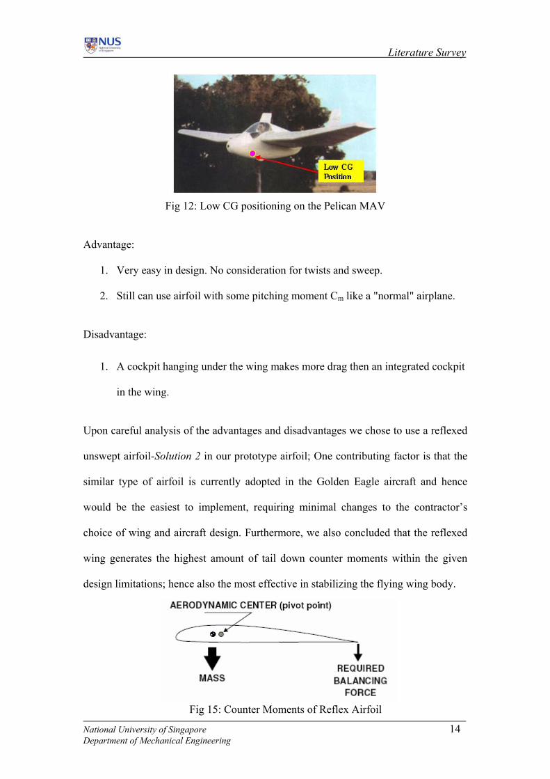
Fig 12: Low CG positioning on the Pelican MAV

Advantage:

1. Very easy in design. No consideration for twists and sweep.

2. Still can use airfoil with some pitching moment Cm like a "normal" airplane.

Disadvantage:

1. A cockpit hanging under the wing makes more drag then an integrated cockpit

in the wing.

Upon careful analysis of the advantages and disadvantages we chose to use a reflexed

unswept airfoil-Solution 2 in our prototype airfoil; One contributing factor is that the

similar type of airfoil is currently adopted in the Golden Eagle aircraft and hence

would be the easiest to implement, requiring minimal changes to the contractor’s

choice of wing and aircraft design. Furthermore, we also concluded that the reflexed

wing generates the highest amount of tail down counter moments within the given

design limitations; hence also the most effective in stabilizing the flying wing body.

National University of SingDepartment of Mechanical

Fig 15: Counter Moments of Reflex Airfoil
apore 14 Engineering

Theoretical Analysis of Airfoil Aerodynamics

Chapter 3: Theoretical Analysis of Airfoil Aerodynamics

3.1 Aerodynamic Forces and Coefficients

Figure 14: The 4 main forces on the airfoil

Lift is the force acting at 90 degrees to the relative airflow as a result of the air

flowing over an aerofoil, whilst drag is the air resistance opposing the direction of

airflow. Lift and Drag forces depend on size, shape, attitude, fluid properties, and

velocity. In addition to the shape and attitude of the body, the surface roughness also

has an effect on these forces.

Fig 15: Flight Angle Definition



This comprehensive factor in the Lift equation is termed the coefficient of lift, CL

represented by the equation,

Likewise for the force of drag,



3.2 Aerodynamic Moments and Pitching Moment Coefficients

Figure 16: The Moments on an airfoil

Moments occur when the c.g is not placed directly above the a.c, hence generating

either a nose down or tail down turning moments shown by the equation,

. In the case of a tailed aircraft not much attention is paid to the airfoil pitching moment

coefficient, Cm. A specific airfoil is selected usually because of performance criteria

and stall characteristics and the negative (nose down) pitching moment is tolerated as

a necessary evil. Horizontal stabilizers with large moment arms can be easily used to

neutralize the moments. But in our case, the Cm value has to be minimal and made

positive, meaning no residual negative pitching moments, giving us a neutral and

inherently stable airfoil shape throughout flight.

3.2.1 Effect of camber on Cm.

Thin-Airfoil Theory determines that the pitching moment generated is dependent

almost entirely on the camber and the distribution of camber of the airfoil. It requires



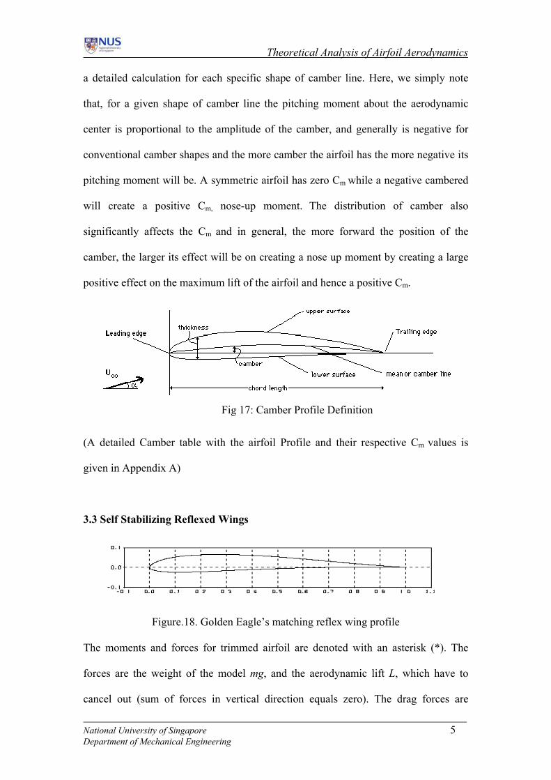
a detailed calculation for each specific shape of camber line. Here, we simply note

that, for a given shape of camber line the pitching moment about the aerodynamic

center is proportional to the amplitude of the camber, and generally is negative for

conventional camber shapes and the more camber the airfoil has the more negative its

pitching moment will be. A symmetric airfoil has zero Cm while a negative cambered

will create a positive Cm, nose-up moment. The distribution of camber also

significantly affects the Cm and in general, the more forward the position of the

camber, the larger its effect will be on creating a nose up moment by creating a large

positive effect on the maximum lift of the airfoil and hence a positive Cm.

(A detailed Camber table wi

given in Appendix A)

3.3 Self Stabilizing Reflexed

Figure.18. Gol

The moments and forces for

forces are the weight of the

cancel out (sum of forces in

National University of Singapore Department of Mechanical Enginee

Fig 17: Camber Profile Definition

th the airfoil Profile and their respective Cm values is

Wings

den Eagle’s matching reflex wing profile

trimmed airfoil are denoted with an asterisk (*). The

model mg, and the aerodynamic lift L, which have to

vertical direction equals zero). The drag forces are

5 ring


neglected here. The sum of the moments around c.g. (caused by the airfoil moment M

and the lift force L, acting at a distance from c.g.) must also be zero.

conventional airfoil with camber airfoil with reflexed mean line

Equilibrium State

This airfoil has a nose heavy moment. The

center of gravity is also the center of

rotation of the wing. When it is located

behind the aerodynamic centre, ac point, the

air force L* in front of the c.g. counteracts

the nose heavy moment M* to achieve

equilibrium.

The reflexed camber line makes the

moment coefficient positive, which means,

that the moment around the ac point is

working in the tail heavy direction.

Therefore the center of gravity has to be

located in front of the ac point to balance

the moment M* by the lift force L*.



Disturbed State

When the angle of attack is increased (e.g.

by a gust), the lift force L increases. Now

L>L* and the tail heavy moment due to the

lift is larger than the moment around ac,

which still is M=M*. Thus the wing will

pitch up, increasing the angle of attack

further. This behavior is instable and a

tailplane is needed to stabilize the system.

Here, we have the air force acting behind the

c.g., which results in an additional nose

heavy moment, when the lift increases. With

L>L*, the wing will pitch down, reducing

the angle of attack, until the equilibrium

state is reached again. The system is stable.


Theoretical Analysis of Airfoil Aerodynamics 3.4 Coupled Control Surfaces

Meanwhile, another important consideration for flying wings is the evolution of

Elevons, which are the coupled and only control surfaces in the absence of Elevators

and the Rudder for a flying wing platform.

Fig 19: Elevons indicated by Yellow arrows

Elevons control the flying wing’s movement in the pitch, yaw and roll axis during

flight. They conveniently replace the bulky tail section and require only two servos

to operate, thus reducing the overall flight weight of the flying wing aircraft.

ELEVATORS + AILERONS = ELEVONS


Preliminary CFD Analysis

Chapter 4 Preliminary CFD Analysis

4.1 Rationale behind the need for CFD Analysis

To understand the characteristics of an airfoil, we need to know the precise

aerodynamic forces of lift, drag and the aerodynamic pitching moments. The Golden

Eagle airfoil we have in hand is currently with no such data, hence, impossible to

study and analyze. Also with the aerodynamic coefficients, the Equations of motion

can be derived by substituting them into these equations. From these equations, the

reactions of the aircraft to specific inputs are known hence enabling us to design a

specialized control system for the Golden Eagle. Conventionally, wind tunnel testing

is done on the model with strain and pressure gauges and velocity indicators attached

all around the airfoil. This allows the aerodynamic forces and moments to be

experimentally measured and subsequently the coefficients computed. But we adopted

another simpler but still equally reliable and less expensive method, given the scope

of out Final year Project– Computational Fluid Dynamic Simulation.

Prior to this, an accurate CAD model needed to be generated. One which we could

mesh and use for our various CFD simulation runs, simulating different wind speeds

and angles of attack.

But with almost no specifications on the camber or spanwise curvature of this highly

unconventional airfoil, creating a CAD model could not just be done from external

physical measurement of the wing. Hence, a reverse engineering routine was

established to profile this airfoil.



4.2 Airfoil Profiling

4.2.1 Laser Profile Photography

Using the Minolta, VIVID 900, Non-Contact-3D Digitizer Image Laser scanner, we

photographed the entire wing profile and fuselage with a tolerance of ±1.5 mm. Each

Wing section had to be photographed from at least six angles all around so that we

could register the appropriate merging points for assembly later. The glossy surface of

the wings had to be matted down with a fine layer of powder dusted through out. The

Laser beams are absorbed by black surfaces; hence to get a proper edge definition, we

photographed the sections against a black back drop. As the edges of the original

Golden Eagle airfoils were painted with a black strip, we inevitably lost some edge

details. But this was overcome in the assembly process.

NatDep

Figure.20. 3-D Laser scanning and Reverse aerofoil CAD modeling procedure

ional University of Singapore 10 artment of Mechanical Engineering


The photographed mesh shells were then merged using the commercial scan

programme RapidFormTM 2002- Reverse Modeler Version. Working with the

photographed scattered points, we had to systematically connect each coordinate to

attain the complex curves on the wing. Plot linearization and CAD editing was needed

to marginalize the inaccuracy inherent in scanning. As we were primarily in search of

the curvature coordinates, we were not too concerned about the inaccuracy along the

edges of the wing which could be manually obtained by paper tracing and plotting.

4.2.2 CAD Modeling

The commercially available CAD software, Solidworks™ was used to edit the points

to form a completed 3D model. The side profile of the fuselage end of the wing was

traced and plotted out on paper. Coordinates at intervals of 5mm were assigned,

measured and input into Solidworks. Nextly, with the sectional camber coordinates

from the laser digital photographs we were able to create a guide curve by which we

could loft the root end of the airfoil to the tip end. This procedure is repeated for the

winglet, for which we also know the angle of inclination from the laser images, with

the exception that instead of a guide curve in this case, a straight line was used to loft

the winglet up to the tip.

The fuselage was more straight forward to model in that it did not consist of any

complex geometry. The fuselage was assumed to be a box with a rectangular-base and

a top that followed the curvature of the wing roots. The nose was also modeled using

simple interpolation curves based on physical measurements.

The control surfaces (elevons) were modeled separately and assumed to be flat

rectangular pieces that could be rotated in the CAD model to simulate deflections.




Figure.21. CAD drawing of the UAV

4.3 Performing the Preliminary Analysis

4.3.1 Preparation of CFD Mesh

The final CAD model was converted into

GAMBIT a mesh preprocessing program. A

different sizes to determine which mesh wo

compromise on computational capacity a

unstructured distributed triangular mesh, w

boundaries of the control volume and dens

surfaces of the airfoil. Usually, a finer mesh

CFD calculation, but it is more computa

Therefore, we used an axis-symmetrical

adapting the mesh, till the solution converge

Figure .22. CAD model of the UAV

a STEP file format and meshed using

mesh analysis was done using meshes of

uld give the most accurate result without a

nd time. The model is meshed with an

ith courser mesh elements near the wall

er meshing at the leading, top and bottom

would give the most reliable results for a

tional expensive and thus not efficient.

model and conducted several runs re-

d and displayed mesh independence.

Figure 23: Meshed Model of the Golden Eagle

12


One of the problems encountered was the skewed edges that the CAD model when

imported to Gambit. Skewed edges are formed when large and long surface converge

to line creating a sharp extended edge like the ones found on the trailing edges of our

airfoil. The preprocessor has an extremely stringent condition for meshing and it did

not recognize parts assembled in external CAD programs. Hence we actually had to

do considerable mesh “tidying” in Gambit by exercising node and mesh control on

these problematic edges.

4.3.2 Simulation Model

Prior to the calculations, a calculation on the UAV’s Reynold’s Number (Re) was

done to investigate whether the flow over the airfoil would be considered laminar or

turbulent. As µρudRe = , we would need to estimate the density (ρ) and the viscosity

(µ) of the air flowing over the airfoil. The velocity of air over the airfoil (u) is

assumed to be constant at 10m/s, which is the cruise airspeed specification given to us

by the manufacturer, and the characteristic length is taken to be 0.77m, the overall

length of the given UAV. Air at atmospheric pressure and the density is taken to be

1.1774 kg/m3 and the viscosity was found to be 1.8462 x 10-5 kg/ms at 300K.

Therefore, the Reynold’s number is:

µρudRe = =

10x1.8462 0.77 x 10 x 1.1774

5-

= 4.91 x 105

The actual value of a critical Reynolds number that separates laminar and turbulent

flow can vary widely depending on the nature of the surfaces bounding the flow and



the magnitude of perturbations in the flow. Since there is very limited knowledge

about the aerodynamics of mini-flying wing UAVs today, we had no tangible

platform to compare our Re number. Given, the subsonic speed of 0.33 Mach we

neglected compressibility effects and used the simple Laminar flow assumption for

the initial simulations. (Results displayed in Appendix A)

Evidently, from the first few runs, we noted that the drag force was unrealistically low

and later via verification through glide tests discovered that the lift force and hence

the CL/CD ratio was also inaccurate. Sighting the turbulence conditions that we test

and fly our aircraft in, and due to fabrication constraints, the airfoil constructed had

considerable surface irregularities, especially on the bottom side. From readings on

low speed aerodynamics, this factor should be sufficient to trigger an early transition

from laminar to turbulent flow. Hence, a suitable computational turbulence model

must be selected and used, because of the high possibility that turbulent, rather than

laminar, flow separation would occur the air foil. Also the practical environment

where the Golden Eagle operates in real life missions encounters much wind hence

reassuring us that the influence of turbulence must not and cannot be ignored.

From the Notes on Numerical Fluid Mechanics, modeling of flow separation for

aerofoils at low Reynolds number, we realized that Turbulence modeling in any detail

is an extensive subject and hence could not be covered in detail for this project. The

key to successful modeling of turbulent boundary layer flow is the selection of a

correct turbulent model. In any case, the turbulent models possible are limited by

those available within Fluent 6, which were state-of-the-art.




A K-Epsilon (RNG) model was used as the K-Epsilon method [19] has been generally

used for turbulence modeling problems. Although another method which requires a

lower computational time is available (Spalart-Allmaras model), it is a one-equation

model, and thus the results would not be as accurate. The RNG K-Epsilon model [20]

was used as it incorporates a formula for lower Reynolds number effects. Along with

other features, it serves as a better model than the normal K-Epsilon model

particularly in our project where we got consistent results that were later verified

experimentally to be rather precise.

4.3.3 Relevant Parameters

Numerical Scheme: 2nd Order Upward Scheme

Viscous Model: Turbulent Setting

Element Type: Triangular

Grid Size: Cells: 75918

Element Size: 2-10 mm

Fluid Type: Air with ρ = 1.1774 kg/m3 and µ = 1.8462 x 10-5

BCDs : – Inlet: Constant velocity

– Side : Axis-Symmetry

– Upper and lower: Periodic setting

Figure 24. 3D-Control Volume

11m

16m


4.4 Results and Discussion

The CFD runs were done with a wind angles ranging from 0 – 50 degrees and

velocities ranging from 10 to 50 m/s, hence simulating the variety of Angle of attacks

of the aircraft. The of CD and CL results of each run was tabulated and were later

experimentally verified through glide tests.

Table 1: The Turbulent Flow CFD computation results

Figure 25. CFD Plot of Pessure Distribution over aircraft

Speed CD CL Cm Drag/N Lift/Kg Mm/Nm 10 0.034291 0.202584 0.01685 0.78301 4.625796 0.38483 20 0.027019 0.218947 -0.01683 2.158994 17.49541 -1.34516 30 0.024746 0.2175 -0.01666 4.449182 39.07617 -2.99512 40 0.020578 0.189608 -0.01452 7.518128 69.27213 -5.30538 50 0.019868 0.189142 -0.01447 11.34138 107.9715 -8.25977

AOA CD CL Cm Drag/N Lift/Kg Mm/Nm 0 0.034291 0.202584 0.01685 0.78301 4.625796 0.384834 10 0.03008 0.578148 -0.03617 0.686844 13.20143 -0.82592 20 0.023966 0.926144 -0.04659 0.547247 21.14759 -1.06374 30 0.029058 1.223494 -0.05519 0.663513 27.93727 -1.26012 40 0.060669 1.290129 -0.08314 1.38532 29.45881 -1.89852 50 0.070256 1.279707 -0.10333 1.604231 29.22084 -2.35938



CL vs Angle of Attack

0

0.2

0.4

0.6

0.8

1

1.2

1.4

0 0.1 0.2 0.3 0.4 0.5 0.6

AOA in radCL

Coefficient of Drag vs Angle of Attack

0

0.01

0.02

0.03

0.04

0.05

0.06

0.07

0.08

0 10 20 30 40 50 60

AoA in degrees

Cd

Graph of CL/CD vs Angle of Attack

0

10

20

30

40

50

0 5 10 15 20 25 30 35 40 45 50 55

CL/

CD

AoA in degrees

Coefficient of Moments vs Angle of Attack

-0.08

-0.06

-0.04

-0.02

0

0.02

0.04

0 10 20 30 40 50 60

Cm

AoA in degrees

These theoretically obtained Forces and Moments were later verified in glide tests

(Chapter 8) to be very accurate and reliable enough to be used for the next stage of

our project, the derivation of stability derivatives for optimizing flight controls.

Figure 26: Polar Plots of Aerodynamic Coefficients

When graphed vs. velocity, these parameters can show you if an aircraft has enough

lift to fly and we can identify a flight speed range. The "lift polar" shows the lift

coefficient CL, plotted versus the angle of attack. From this we found that the CLmax of

the airfoil was 1.295 and the corresponding angle of attack to be 37-39 degees,

beyond which the stall behavior of the aircraft comes to play. This is significant as we

now have successfully identified the flight envelope of this airfoil for high angle of



attack flight. Hence, the aircraft would stall and start to drop like a stone, when it

reaches angles of attack above 39 degrees. (Evidence of this behavior has been

recorded on video during flight testing).

The lift against velocity curve shows the speed required to maintain flight. It was thus

found that the Golden Eagle could generate a lift force of 4.646 N at a cruise speed of

10 m/s and encountered a turbulent drag of the magnitude of 0.783N.

• Maximum specified flight weight of Golden Eagle :1200g

• Targeted Equipment load (Autopilot,GPS, Camera etc) : 250g

• Lift Force calculated at 10 m/s : 4646g ×9.81 N

• Required Thrust to overcome drag at 10m/s: > 0.783 N

Hence, with the detailed lift characteristics of the aircraft identified, we discovered

that it can actually carry approximately 4 times its specified load and still fly without

stalling or crashing. The drag force at this speed also guided us in propulsion

sizing(Chapter 9), ensuring the trust force that the new power plant provides can

overcome the induced drag and provide a speed range of between 10 -15 m/s for

straight and level flight.

Having high thrust/weight and lift/drag ratios are not enough to guarantee that a plane

is capable of steady flight. Without properly balanced moments about the craft’s

center of gravity even the smallest of perturbations to the vehicle’s flight path can

potentially send the plane tumbling out of control. (CG balancing done in Chapter 6).


Prototype Fabrication

Chapter 5: Prototype Fabrication

5.1 Reason for Reverse Prototyping

The physical replica of the UAV is required as damage is foreseen during the flight-

testing phase. It would be unwise to damage the original given model, as it is very

expensive. Unable to match this particular wing with any of the standard NACA

airfoils present, we had to generate a full 3 Dimensional CAD model of the craft from

scratch. Also, the simplistic construction drawings provided could not accurately tell

us the wing curvature at the concave leading edge and at the convex trailing edge.

Construction of the wing and fuselage were one of the toughest challenges we faced.

We wanted our wing to be as smooth and accurate as possible. Also, an easily

repeatable wing fabrication process could help us during flight testing in case the

wing was damaged beyond repair and a new wing needed to be made. These features

require a Reverse prototyping process, where we construct molds and tools

specifically to re-construct the golden Eagle airfoil. This is almost the exact opposite

design principle, where we dimension an existent airfoil and then design the

procedure to build it.. Since the fuselage is home to all of the expensive components,

it needs to be built strong enough to protect the equipment inside during an impact.

Strength, light-weight, and low-cost are nearly contradictory terms. Only a few

materials available to us were considered. Among them were carbon fiber, glass fiber,

foam and balsa wood.



5.1.1 Model Dimensioning

The model was then sectioned and sliced at critical intervals to obtain the exact

structural coordinates to be used to design and construct the wings.

Figure.27. Eleven Sectioned ribs along the Wing

The fuselage dimensions were easily measured externally, as it did not contain any

complex geometries.

5.2 Material Research and Selection

The original Golden Eagle wings were made of Kevlar composite fibers. Kevlar is a

very light and extremely strong and tough material. But unfortunately, it is very costly

and could not be purchased in small quantities. Material research had to be done to

find an equally durable and light material to build our prototypes for testing. Because

design development was heavily dependent on flight-testing, the ease, speed, and

precision of manufacturing and repair was a fundamental consideration about the

materials chosen and the manufacturing procedure adopted. All components were

deliberately determined to be modular and are meant to break away during impact.

This ensures minimal damage by allowing us to localize the damage to easily

replaceable components (e.g the nose), hence reducing repair costs and time.



Traditional ways of making wings involves making reinforced cross-sectional spars

covered with a plastic, heat-shrinking material or some other similar type of covering.

Some problems with this design are its inaccuracy and its fragility. Also,

aerodynamically speaking, the form of the airfoil is greatly compromised for the

sections of the wing that lie in between the spars.

Although balsa wood and foam are conventional materials, they could not be adopted

here due to the complex and unconventional airfoil shape (distributed camber) that we

had to model and also due to the non-availability of precise contour machining tools.

Various materials such as low and high density foam, stiff ¼-1/2 in. cardboards, paper

march’es and laminate resins together with different manufacturing processors were

experimented with initially, primarily due to their ease of availability and extreme low

cost. But unfortunately, they were either too heavy or not rigid enough to take the

required wing loading. Hence we started looking into composites as a viable

alternative. A comparison was made between different types of fibres and resins to

choose the suitable one in terms of pricing, weight and mechanical strength.

Table 2: Comparison of Fiber properties (Ref: Hull & Clyne)

Cost Density (Mg/m3) Tensile Strength (GPa)

Carbon Mat High 1.95 2.4

Glass Mat Low 2.56 2.0 Kevlar Mat High 1.45 2.3

Table 3: Comparison of Resin properties (Ref: Hull & Clyne)

Cost Density (Mg/m3) Tensile Strength (GPa)

Polyester Low 1.3 40-90

Epoxy High 1.2 35-100



Finally, we singled out single ply bi-directionally laid tissue glass fiber (GFRP) as

GFRP combined the mechanical properties of both the plastic resin as well as the

strengthening fibers to give high rigidity, superior strength-to-weight ratio and

displayed excellent mechanical properties upon impact-a crucial consideration for a

UAV without landing gear mechanisms. It is also low in cost and readily available.

5.3 Structural Construction

5.3.1 Tissue Fiber Laying

Reusable male and female clay molds were created and checked for consistency

against the acquired wing curvature dimensions. The glass fiber framework was then

laid on the molds and covered with a thin layer of synthetic polymer (Ethylene

Glycol, wt. % 99.9 - Polyester). Specifically measured quantities of resin were applied

equally on each of the two wings, maintaining symmetry in weight. The viscous resin

was poured down on the wing, with the mold propped vertically up. This ensures an

even distribution of resin throughout the cast. It was then allowed to drip and air dry

in an enclosed area. This procedure gave a smoother and more even exterior finish

compared to the conventional method of brushing on the polyester. The entire

manufacturing process is highly repeatable with the usage of durable and reusable

le materials.

molds and cost effective readily availab

igure.28. Pouring of the resin Figure.29. GFRP right wing bottom shell

F




Figure 30: Assembled ribs

Fibre Wing



Figure 30: Assembled ribs

Fibre Wing

as sed to create the two

transitions along the lateral

he fuselage is built with light weight balsa wood hollowed out to house the

5.3.2 Wing and Fuselage

A hand lay-up method w u

bottom halves of the UAV’s wings. Via dimensional

slicing we had the exact profile of sectional ribs

which we cut out on balsa ply. Sections of the wing

(closer to the fuselage) that had a high degree of

span-wise curvature had more ribs assigned while

those closer to the wing tips had fewer. This

distributed method, allowed a more accurate

modeling of out M-shaped wing allowing smoother

curves. A thin layer of film is then wrapped onto the balsa wood profiles and the

fiberglass bottom to give the complete airfoil shape.

T

equipment, and the modular nose section was made out of High density foam, capable

of deforming and absorbing shock during impact. The nose was carefully anchored to

the fuselage using pins that easily cut through the balsa fuselage, allowing the nose to

break away during impact. A similar approach was used by employing short carbon

rods as interfaces when attaching the wings to the fuselage.

5.4 Assembly

Figure 31: Assembly LayoutFigure 31: Assembly Layout

Modular Nose Modular Nose

Propellhousin

er g

Propellhousin

er g

23

23

BatteryhousingBatteryhousing

Carbon Carbon Rods Rods

Balsa Ply Elevons

Estimation of CG Position and MOI

Figure 32: CG Balancin

Table 4: Componen

Chapter 6: Estimation of CG Position and Mass of Inertias

.1 Aerodynamic Centre and Estimation of CG Position

Moment Contribution for the payload

6

Mo oad = -0.3815 Nm

Moment Coefficient of Airfoil = 0.01685

Balanced manually with bal

The eq

balance out the residual moments we discovered in

our CFD analysis. Due to the symmetrical design of

the aircraft, we concentrated only on the longitudinal

positioning of the cg. Laterally, the craft was found to

be off-balanced by a few grams (11g) when we

experimentally balanced the craft on a pivot. But this

was unavoidable, given our fibre laying technique and

the vicious e resin used. But, this was easily resolved by manua ng

wing with ballasts. (Extended Mass Table in Appendix G)

• Total ment For Payl

•

• Moment of Airfoil = +0.3848 Nm

• Residual Nose-up Moments = 0.003 Nm (

uipment was strategically placed in the fuselage

to

Pusher Propeller Un

lly off-setti

Radio control electronics (two servmotors, servo card

RC receiver) Video electronics

(camera, transmitte

Batteries (9-volt, 50mAh NiCd)

Micro Pilot Card &Cables

Structure

Total

m

0.300 0.06

m


0.77
cg
0.395
0.03 0.72 0.74
0.029kg Micro Pilot

0.45kg tteryBa
0.055kg
C meraa
0.145kgMotor
0.065kgServos
0.005kg
opellerPr

0

g Chart

t Weights

last)

the ri

it

ght

150g

o ,

65g

r) 55g

350g

29g

800g 1569g

24


Via the above theoretical

estimation method, we found that the c.g is located 0.395m

We also know that the CG must be located ahead of the ac, if we want a self

stabilizing wing as the profile we are using is reflexed.

from the tip of the nose.

onditions must be met for longitudinal stability.

The validity of this expression is easy to see: as an increased pitch angle should be

ounteracted with a negative nose down pitching moment. The root airfoil has a

compared ).

Stability is a very important criterion in the design of aircraft. For flying wings, two

c

0&0 >< mm CC α

c

pitching moment near zero; hence the normal down force required by the wing tips is

not great. As shown in our Cm vs α CFD curve, is that the gradient is negative

0<αmC and the graph intersects the x-axis on the positive end 0>mC .

Furthermore, the Cm values for this unconventional airfoil are much lower than those

with conventional airfoils of similar configuration. (In Appendix F

0434.00911.0−=

0985.2−

=αα

CL

The Cmα / CLα calculation tells us where our aerodynamic centre lies, the point where

the moment acting on the body is independent of the angle of attack, and since this is

Cm

a flying wing with a comparatively small central fuselage which also rides the wing

profile, we conclude that the neutral point too lies at the AC location calculated. The

negative value tells us that the AC actually lies behind the CG location by 0.0434m.



26

g National University of Singapore Department of Mechanical Engineerin

Figure.33. Location of AC with respect to the CG To experiment method of CG

etermination was employed - the entire assembled model was mounted on a self

Figure.34. Experimental verification of CG position

he experimental verification proved to be almost exact.

ally verify our calculations, the conventional

d

constructed level pivot, with a broad and sharp edge, and shifted accordingly to attain

the mass centre of the individual components.

T

Theory= CG located 395mm from the Nose tip

Experiment= CG located 392mm from Nose Tip

-0.0434m

3mm of discrepancy


6.2 Static Margin

Static margin is the distance between the c.g and the neutral point which is the AC in

y. If the c.g is ahead of the AC, then the static margin is positive,

.g ahead of AC = +0.0434m

our flying wing bod

and the static stability is positive by an amount that is related to the static margin. If

the AC is behind the neutral point, then the static margin and static stability are

negative (i.e. the model is statically divergent, if you pull the nose up it pitches up

even more).

Mean aerodynamic chord, MAC = 0.465m (Geometrical derivation in Appendix E)

Static Margin Calculations,

c

% 33.9% 100465.0

0434.0×Static Margin = = of MAC

The equations for moment of inertia, are also referred to as “second moment”

equations. This is due to the squared moment arm that multiplies each infinitesimal

distance is y + z .

6.2 Mass of Inertia Estimation

volume during the integration. In the case of the Ixx

, the distance from the x-axis is the

moment arm to be squared, and due to the Pythagorean Theorem, this squared

2 2

The same method is used for the other moments of inertia. But in order to safe

e integration, we can approximate the Inertias with the

geometric summation of the various components of different masses in the structure,

computation effort in extensiv



as per equations (1)-(6) (Ref: Jon Roskam). We must assume that each component has

a constant density and mass distribution throughout. The detailed integration formulae

are illustrated in the appendix D.

( ) ( ) =

=

=

=

++−=

ni

i

ni

iZcgZiYcgYimiIxx

1

1

22

( ) (

( ) ( )

( ) ( )

( ) ( )

( ) ( ) ∑

∑

∑

∑

∑

∑

=

=

=

=

=

=

=

=

(1)

)

−−=

=−−=

=−−=

−+−=

−+−=

ni

i

ni

i

ni

i

ni

i

XcgXiZcgZimiIzx

ZcgZiYcgYimiIyz

YcgYiXcgXimiIxy

YcgYiXcgXimiIzz

XcgXiZcgZimiIyy

1

22

1

22

1

22

1

22

22

0

0

Symmetrical Aircraft

(2) (3)

)

)

)

(4 (5 (6

Figure.35. Geometrical Estimation of Inertias



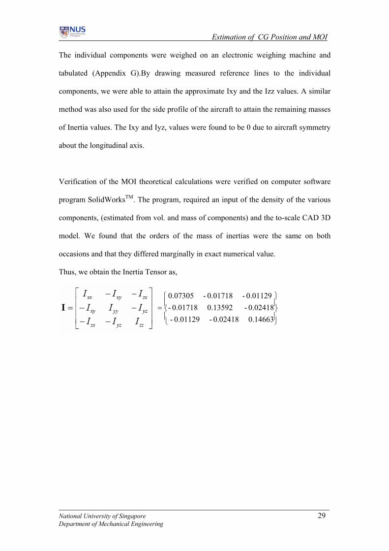
The individual components were weighed on an electronic weighing machine and

tabulated (Appendix G).By drawing measured reference lines to the individual

components, we were able to attain the approximate Ixy and the Izz values. A similar

method was also used for the side profile of the aircraft to attain the remaining masses

of Inertia values. The Ixy and Iyz, values were found to be 0 due to aircraft symmetry

about the longitudinal axis.

Verification of the MOI theoretical calculations were verified on computer software

program SolidWorksTM. The program, required an input of the density of the various

components, (estimated from vol. and mass of components) and the to-scale CAD 3D

model. We found that the orders of the mass of inertias were the same on both

occasions and that they differed marginally in exact numerical value.

Thus, we obtain the Inertia Tensor as,

⎫⎧ 0.01129 - 0.01718- 07305.0

⎪⎭

⎪⎬

⎪⎩

⎪⎨=

0.14663 0.02418- 0.01129- 0.02418- 0.13592 0.01718-


Glide Tests and Verification

Chapter 7:Glide Tests and Verification

7.1 Preliminary Glide Test

7.1.1 Glide Test Theory

Ω

h

National University o 30 Department of Mechanic

f Singapore al Engineering

Figure.36. Glide Slope Angle definition

7.1.2 Experimental Set-up and Calibration

We needed an elevated platform e time be able

identify it’s glide slope.

d

eld as our launchi

latform. The plane was

to launch the craft from and at the sam

to

Hence, we chose a test

site with an incline

measurable slope that

opened up into a wide

fi ng

Figure.37 Glide Test Grounds

p

3.203m


to

be hand launched at zero angle of attack and at an approximate velocity of 10m/s.

wo video cameras were set up on stands to help gauge the glide slope (one on each

ide of the glide slope).

field and we aligned our launches along

Furthermore, the slope we launched from had a flight of

green railings of stairs, seen in picture above), and this

nch height.

d and to regulate

throughout the

n simplistic speed

spool has a reflective

pe stuck to it, so that we can read its rpm

also allows it to get dislodged easily if the

nsion is too great.

T

s

There was a parallel path running, along the

this path. This was primarily because; we could later use it as a straight gauge to

measure the glide distance.

stairs running alongside it (

served us in measuring the lau

To measure the launch spee

the speed as a constant

experiment, we built our ow

gauge. It consists of an anchored spool of

thread stuck to the bottom side of the

fuselage. The side of the

ta

with a tachometer. The total length of the

thread is 12 meters, and once the aircraft travels further then 12 meters, it gets

dislodged from the spool and follows the craft. The spool is free rotating and the

thread used is very light, causing negligible resistance during flight. The loose method

of attaching it to the aircraft with a tape

Spool

Figure 38: Speed Measurement Setup

te



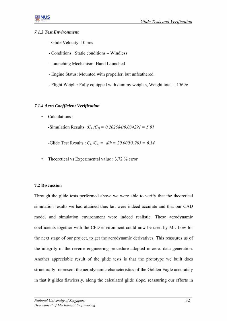
7.1.3 Test Environment

- Glide Velocity: 10 m/s

- Conditions: Static conditions – Windle

- Launching Mechanism: Hand Launched

- Engine Status: Mounted with propeller,

- Flight Weight: Fully equipped with du

7.1.4 Aero Coefficient Verification

ss

but unfeathered.

mmy weights, Weight total = 1569g

-Glide Test Results : C /C = d/h = 20.000/3.203 = 6.14

Experimental value : 3.72 % error

7.2 Discussion

Through the glide tests performed above we were able to verify that the theoretical

simulation results we had attained thus far, were indeed accurate and that our CAD

model and simulation environment were indeed realistic. These aerodynamic

coefficients together with the CFD environment could now be used by Mr. Low for

the next stage of our project, to get the aerodynamic derivatives. This reassures us of

the integrity of the reverse engineering procedure adopted in aero. data generation.

Another appreciable result of the glide tests is that the prototype we built does

structurally represent the aerodynamic characteristics of the Golden Eagle accurately

in that it glides flawlessly, along the calculated glide slope, reassuring our efforts in

• Calculations :

-Simulation Results :CL /CD = 0.202584/0.034291 = 5.91

L D

• Theoretical vs



the structural reverse engineering procedures adopted too. Finally, we were able to

prove t matching done, the

Go n out 260g.

ith, these results we were certain that our project had indeed progressed in the right

and our main efforts now would be in propulsion research and

hat with the correct c.g positioning and weight and balance

lde Eagle could in fact carry in access a payload of ab

W

direction so far

selection to provide sufficient lift generating thrust for straight and level flight.


Propulsion System and Integration

Chapter 8: Propulsion S tem Integration ys

8.1 Propulsion Systems

8.1.1 Theoretical Analysis

Generation of thrust during flight requires the expenditure of power. In steady level

rust is equal to the aircraft drag.

Power ≡ Thrust x Vel. = Drag x Vel.

Similar to airfoils and wings, the performance of propellers can be described by

imensionless (normalized) coefficients. A propeller is described in terms of advance

ratio, thrust coefficient, and power coefficient. The relevant equations are as follows,

Thrust

flight, the th

d

Power

Advance Ratio

Efficiency

Where,

v velocity m/s D diameter m

dn revolutions per secon 1/s density of air

kg/m³ P power W T thrust N

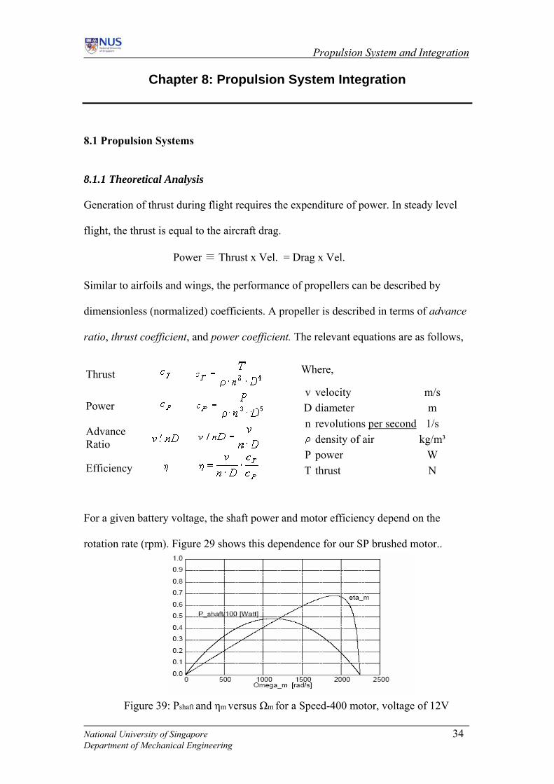
the shaft power and motor efficiency depend on the

rotation rate (rpm). Figure 29 shows this dependence for our SP brushed motor..

Figure 39: Pshaft and ηm versus Ωm for a Speed-400 motor, voltage of 12V

For a given battery voltage,



35 National University of Singapore


The propeller then converts the shaft power to thrust power as such,

P = ηp Pshaft = ηp η

W easure the electrical power utput,

t that woul still require us t otor efficiencies.

us f otor vendors, we opted to

irectly measure the trust force with our own experimental set-up.

Procedure: 1) We tested two motor units primarily, the Himax--- and the SP ---

2) Each with 5 different pusher propellers of various pitch and diameter

rotating moments are measure for 3 thrust settings

4) Voltage drawn per thrust setting is also measure with a voltmeter

5) Airspeed behind the propeller is also measure with an anemometer

m Pelec

e could m o the motor rpm and the shaft power

inputs, bu d o know the propellers and m

Since this data was not readily available to rom the m

d

8.1.2 Experimental Set-up

0.50

Propeller Unit

0.25m

Figure.40. Thrust measurement: Test Stand Setup

3) The downward

6) Results are tabulated and discussed


8.1.3 Analysis of Data

oals: 1) Selecting correct Electric motor and propeller combination

2) Power requirements on board (Number of batteries needed)

he calculations involve moment balancing,

easured weight x 0.5 x 9.81(g) = Thrust x 0.25

Table 3:Thust experimental results

Extended tabulation of voltage, airspeed and moments are shown in Appendix B.

type of

prope creased

proved to be a more significant

Thrust formula. We chose

Air screw pusher

propeller with a pitch of 6, because it was lighter and also delivered the

highest thrust at all power settings and could overcome drag forces

encountered by the craft up to angles of attack of 40 degrees. It also proved

to be the most efficient, in terms of battery power consumption. It ran at

G

T

M

Thrust (N) Motor Prop Idle Mid Max

9x6 0.706 4.571 6.887 8x7 0.471 4.042 5.709 8x4 0.706 4.258 6.416 7x5 0.746 3.551 4.944

Himax .15kg

6x4 0.314 1.844 2.511

9x6 0.530 4.277 6.533

8.2 Discussion

The thrust force generated for the motors depend heavily on the

llers we used. While higher pitched propellers provided an in

thrust, the increase in propeller diameter

factor due to their xD4 factor of influence in the

the Himax motor coupled with the 9 inch diameter,

8x7 0.275 3.826 5.140 8x4 0.530 4.252 6.318 7x5 0.628 3.571 4.768

GS .17kg

6x4 0.177 1.766 2.237

100% throttle setting on 4, 9-volt, 50 mAh NiCd cells for approximately 29 mins.

Figure 41: The 9x6 Pusher Propeller


Flight Testing

37 National University of Singapore


Chapter 9: Flight Testing

9.1 Outdoor Testing:

.1.1 Test Sites

Testing was performed in the following venues.

a) Open air area at Jurong East

b) Open air area at Marina South

du f the

pr t also

pr s the

G soft

gr n.

9.

F -pilot

sy d have

e d,

collected flight velocity and altitude data which we retrieved once the craft landed.

We measured flight endurance by constantly measuring the voltage drop in the

batteries with a multi-meter, each time the plane is grounded. Flight distance is

measure with a measuring tape, from the launch point to the landing site and flight

duration is timed with a conventional stop watch. In addition, we documented every

Powered

9

c) Open field at Ports Down Road Figure 42: High AoA altitude ascend

A large area was sought in order to allow the craft an unobstructed area to maneuver

ring the flight tests. This not only allows a more realistic assessment o

ototypes’ performance and dynamic characteristics on-site on in-video, bu

events the craft from damage when crashing on walls. With no landing gear

olden Eagle prototypes had to either fly into a recovery net or crash land on

ound. Lack of man-power to mend the large nets forced us to use the later optio

1.2 Test Routines

ully integrated with RC control unit, a dummy camera weight and the auto

stem we hand launched the prototype from an elevated terrain, so that it woul

nough ground clearance uto pilot card on boarto glide and climb altitude. The a

Flight Testing

sing ent, which were analyzed in the lab frame by

fram nse of control

9.1.3 Problems

Upon patching the wing of the model, we discovered that it actually altered its

ristics and weight balancing (C.G and Inertia), so we had to

9.2 Test Data Gathered

Test Data Collected: 1) Flight Velocity = 10.6 – 22.3 m/s

2) Max.Flight altitude = 25m above launch ground

3) Flight Weight = 1625g

4) Flight Endurance = 12s

5) Battery endurance = 29minutes

6) Structural stability = Excellent

7) Thrust = >Sufficient

8) Noise Level = < Original

9) Critical Stall Angle = 40-45 degrees

le test attempt with video equipm

e to identify stall angles and respo surface deflections.

Induced oscillations from hand launching, together with inconsistent launch angles,

plagued the initial attempts and caused severe damage to the wings and fuselage of

our first prototype during crashes.

aerodynamic characte

built our second, third and subsequently our forth prototype throughout our extensive

flight test routines. On our other prototypes, we paid greater attention to launching at

a consistent angle of attack, ensuring both proper alignment of the thrust line and

wings in the intended direction of flight.


Flight Testing

9.3 Flight Test Results

Lift Characteristics: 1) Achieved take-off

2) Achieved altitude ascend to 25m

3) Achieved Straight and level flight

4) Increased Payload Margin +260g

This verified that our reverse engineered prototype was structurally and

aerodynamically stable and could gener

ate enough lift to sustain flight. It could also

ortlessly carry the additional payload of 260g and was balanced in the

longitudinal axis, allowing it to attain self stabilized level flight. A recorded flight

ceiling of 25m was also attained.

Thrust Characteristics

eff

: 1) Achieved take-off speed of >10m/s

2) Max AoA 40-45 degrees

3) Straight and level flight

4) Cruise conditions of 8-12m/s

5) Max Recorded Speed 22.3m/s

6) Low motor noise levels

The new propulsion system allowed cruise sustained speeds of 8-12 m/s and also

provided sufficient thrust to overcome drag even during high angled of attack

loops. It also proved to be quieter than the original one and displayed a full throttle

flight endurance of 29 minutes.

Visual evidence of the flight testing is available in video. Interested readers are

requested to refer to the attached CD-R, to obtain understanding of the following

discussion.


Flight Testing

9.4 Discussion

From our flight test we were able to deduce that the structural aerodynamics of the

craft, the propulsion system and

c.g positioning were precise, it that the aircraft

could take-off climb, and fly straight and level. A stable platform which replicates

systems.

Sighting the, slow t perturbations and the rapid

respond rates of the to fly with the aid of the

micro pilot card. To system he designed on

our 4th prototype an ay point (2-point) flight. Once

se results could not be repeated over longer test

o control inputs making it difficult to maneuver in the air.

the Golden Eagle is now available for Mr. Low to test his control

human response to the aircraf

aircraft in the control axis, we decided

gether with Mr. Low, we integrated the

d prepared it for autonomous, w

the aircraft was airborne Mr. Low activated the autopilot routine and proceeded to

test the onboard control system. We were able to see that the aircraft trying to auto

correct itself in the air and we have video evidence of autonomous flight over a

short distance of 50 m, but the

distances. Sustaining stable controlled flight in the presence of wind perturbations

proved to be difficult, even with autonomous flight as it responded extremely

sensitively t

Figure 43: Prototype-Three


Conclusion

Chapter 10: Conclusion

This project has successfully validated the usefulness of reverse engineering in

aerodynamic analysis of unconventional small scale aircraft structures. Through a

realistic CFD environment the CL, CD, and CM values for the Golden Eagle’s

unconventional reflex airfoil were generated and verified via glide tests to be accurate

and consistent. This unrevealed the self stabilizing and increased lift characteristics of

the airfoil design, which are an asset to Cradence Services, who had limited idea of

their airfoil’s characteristics till today. We were also able to completely reproduce the

airfoil structure and prototype four modular, aerodynamically identical replicas of the

UAV, at the fraction of the original cost for testing, and hence incurred no damage at

all to the o

ized by 20-23 %

at flight sp too gave the

correct estim

The propulsion studies sho ller geometry and power

of the motor were crucial in delivering additional thrust. The new propulsion system

finally integrated in the prototypes delivered approximately 3 times more than the

previous attainable thrust effortlessly.

The final integrated aircraft could lift its own weight and fly in a level configuration

and ascend altitude displaying key aerodynamic characteristics. This allowed Mr.Low

riginal expensive model given to us.

Studying the lift and drag polars, the payload margin was duely optim

eeds of 10 m/s. Stability and weight balancing procedures

ates of the centre of gravity, aerodynamic centre and the Inertia tensor,

which could be used by my colleague to establish the equations of motion.

wed that the combination of prope


Conclusion

to establish and test some key characteristics of his onboard control system, in the

context of the prototypes dynamic behaviors.

Throughout this multidisciplinary project we have achieved our objectives by,

• Developing, validating, and applying aerodynamics models for the analysis and design of

realistic, three-dimensional configurations for the aero Industry.

• Understanding the impact of uncertainty and variability on aerodynamic predictions and

the resultant impact on aircraft system performance estimates;

• Computational Fluid Dynamic Simulations;

• Adopting the complimentary roles of theory, experiment, and computations in

aerodynamic analysis and design.

NationDepar

Figure 44: Flight Testing of Protoype-4 with 6x4 Propeller and GS Motor

al University of Singapore 42 tment of Mechanical Engineering

Recommendations

Chapter 11: Recommendations

Future recommendations would include the following steps.

a) Familiarizing oneself with Gambit, the CFD preprocessor supporting Fluent. This

ia or Solidworks as an interface, thus avoiding

erous part file exports and cumbersome “mesh tidying”.

) Wo This

ould allow us to generously fabricate both the bottom and top airfoil shells without

uch concern for weight.

) A mechanical Launcher can be designed and built to allow consistent launching,

ach and every time, at an adjustable Angles of attack and velocity.

e) A less destructive y proper on ground

reparation of recovery nets prior to glide and flight testing.

would be useful in assembling CAD models directly before creating the mesh, without

other CAD programs such as CaT

num

b) Develop more advanced techniques for composite parts construction. Future

students may attempt this as part of an UROP project to support their future FYP

work to ensure sufficient time. Parts that can benefit from this skill include

lightweight fuselages, airfoils and custom-made propellers.

c rking with more leading edge materials such as Carbon or Kevlar fibers.

w

m

d

e

flight test approach can be undertaken b

p


References

List of References

1. Karl Nickel, Micheal Wohlfahrt, “Tailess Aircfracfts in Theory and Practice”, AAA

education Series, 1995

2. Airplane Design, Part V: Components weights estimation. By Dr Jon Roskam,

New York, Cambridge University Press, 1996.

. McGhee, R.J., Walker, B.S., and Millard, B.F., “Experimental Results for the

Pressure Tunnel,” NASA TM 4062, October 1988.

, L.L., “Low-Reynolds-Number Separation on an Airfoil,”

AIAA Journal, Vol. 34, No. 8, 1996, pp. 1570–1577.

European Commission Directorate General XII on Science, Research &

7. Kuethe A.M., Chow C.Y.,“Foundations of Aerodynamics: Bases of Aerodynamic

Design”, 4th Edition, John Wiley & Sons, Canada, 1986

8. Ferziger J.H., Peric M, “Com mics”, Springer-

Verlag, Berlin, 1998.

9. Selig M.S., “Summary of Low Speed Airfoil Data”, Soartech Publications, VA,

Professor of Aerospace University of Lawrence Kansas, Kansas.

3. “D.Hull and T.W. Clyne” An Introduction to composites materials”. Cambridge;

4

Eppler 387 Airfoil at Low Reynolds Numbers in the Langley Low-Turbulence

5. Lin, J.C.M., and Pauley

6. Hasse W, Chaput E, Elsholz E, Leschziner M, Müller U.R. editors, “Notes on

Numerical Fluid Mechanics Volume 58”, Community Research in Aeronautics,

Development; Friedr Vieweg & Sohn,. 1997,

putational Methods for Fluid Dyna

USA, 1995.


References

10. Fletcher H.S., “Experimental Investigation of Lift, Drag and Pitching Moment of

ted, 2001.

nd

16.

ehicle” AIAA 2001-0127, 39th Aero. Sci. Meet & Exhibit,

Reno, NV, USA, Jan. 2001

19. der and D. B. Spalding. “Lectures in Mathematical Models of Turbulence”. Academic Press, London, England, 1972

Five Annular Aerofoils:, Langley Aeronautical Laboratory, Langley Field, Va,

USA, October 1957

11. “Max-Himax, 2825, 32SX Owner Instruction Manual”, Brushless Motors .Mfg

Co.Ltd, Osaka, Japan, 2000.

12. “Gambit 2.0.4 Online Documentation”, Fluent Incorporated, 2001

13. “Fluent 6 Online Documentation,” Fluent Incorpora

14. Beer, Ferdinand P. and E. Russell Johnston, Jr., Vector Mechanics for Engineers,

5th

Ed., McGraw-Hill, New York, 1988.

15. Mortenson, Michael E., Geometric Modeling, 2 Ed., John Wiley and Sons, New

York, 1997.

David C Aronstein & Albert C. Piccirillo, “Have Blue and the F-117A, Evolution

of the Stealth Fighter”, AIAA Inc. 1997

17. Daniel P Raymer, ‘Aircraft Design: A conceptual approach’, AIAA Education

Series, ISBN 1-5634/-281-0, 1999

18. Joel M. Grasmeyer and Matthew T. Keennon, “Development of the Black

Widow Micro Air V

B. E. Laun

20. V. Yakhot and S. A. Orszag. “Renormalization Group Analysis of Turbulence:I. Basic Theory”. Journal of Scientific Computing, 1(1):1-51, 1986


References

21. Navabalanchandran J., Low J.H & Gerard Leng, “Reverse Engineering and

Aerodynamic Analysis of a Flying Wing UAV”, RSAF Aerospace Technology

Seminar, 2005

2. Mueller, T. J. (ed.), Fixed and Flapping Wing Aerodynamics for Micro Air Vehicle Applications, AIAA, Virginia, 2001

3. Simons, M., Model Aircraft Aerodynamics, 4th ed., Special Interest Model Books,

2

2

Dorset, England, UK., 1999


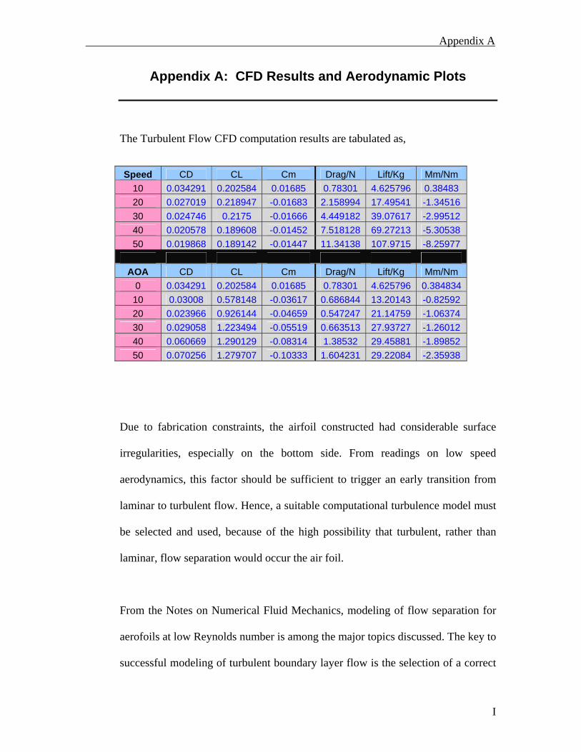
Appendix A

Appendix A: CFD Results and Aerodynamic Plots

The Turbulent Flow CFD computation results are tabulated as,

Speed CD CL Cm Drag/N Lift/Kg Mm/Nm 10 0.034291 0.202584 0.01685 0.78301 4.625796 0.38483 20 0.027019 0.218947 -0.01683 2.158994 17.49541 -1.34516 30 0.024746 0.2175 -0.01666 4.449182 39.07617 -2.99512 40 0.020578 0.189608 -0.01452 7.518128 69.27213 -5.30538 50 0.019868 0.189142 -0.01447 11.34138 107.9715 -8.25977

AOA CD CL Cm Drag/N Lift/Kg Mm/Nm 0 0.034291 0.202584 0.01685 0.78301 4.625796 0.384834 10 0.03008 0.578148 -0.03617 0.686844 13.20143 -0.82592 20 0.023966 0.926144 -0.04659 0.547247 21.14759 -1.06374 30 0.029058 1.223494 -0.05519 0.663513 27.93727 -1.26012 40 0.060669 1.290129 -0.08314 1.38532 29.45881 -1.89852 50 0.070256 1.279707 -0.10333 1.604231 29.22084 -2.35938

Due to fabrication constraints, the airfoil constructed had considerable surface

irregularities, especially on the bottom side. From readings on low speed

aerodynamics, this factor should be sufficient to trigger an early transition from

laminar to turbulent flow. Hence, a suitable computational turbulence model must

be selected and used, because of the high possibility that turbulent, rather than

laminar, flow separation would occur the air foil.

From the Notes on Numerical Fluid Mechanics, modeling of flow separation for

aerofoils at low Reynolds number is among the major topics discussed. The key to

successful modeling of turbulent boundary layer flow is the selection of a correct

I

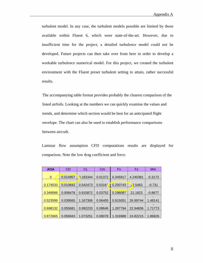
Appendix A

turbulent model. In any case, the turbulent models possible are limited by those

available within Fluent 6, which were state-of-the-art. However, due to

insufficient time for the project, a detailed turbulence model could not be

developed. Future projects can then take over from here in order to develop a

workable turbulence numerical model. For this project, we created the turbulent

environment with the Fluent preset turbulent setting to attain, rather successful

results.

The accompanying table format provides probably the clearest comparison of the

listed airfoils. Looking at the numbers we can quickly examine the values and

trends, and determine which section would be best for an anticipated flight

envelope. The chart can also be used to establish performance comparisons

between aircraft.

Laminar flow assumption CFD computations results are displayed for

comparison. Note the low drag coefficient and force.

AOA CD CL Cm Fx Fz Mm

0 0.014957 0.183344-

0.01372 0.345917 4.240381 -0.3173

0.174533 0.010842 0.542473-

0.03161 0.250743 12.5463 -0.731

0.349066 0.008478 0.915872-

0.03752 0.196087 21.1823 -0.8677

0.523599 0.039565 1.167306-

0.06405 0.915051 26.99744 -

1.48141

0.698132 0.055681 0.992233-

0.09646 1.287794 22.94836 -

1.71773

0.872665 0.056943 1.073251-

0.08078 1.316988 24.82215 -

1.86826

II

Appendix A

Plots of Turbulent Aerodynamic Forces and moments,

Lift Force vs Angle of Attack

05

101520253035

0 10 20 30 40 50 6

AoA in degrees

Lift

N

0

Drag Force vs Angle of Attack

0

0.5

1

1.5

2

0 10 20 30 40 50 6

AoA in degrees

Dra

g N

0

Moments vs Angle of Attack

-2.5-2

-1.5-1

-0.50

0.51

0 10 20 30 40 50 6

AoA in degrees

Mom

ents

Nm

0

III

Appendix A

Lift Force vs Velocity

020

406080

100120

0 10 20 30 40 50 6

Velocity m/s

Lift

N

0

A.1 Simple Momentum Theory

Drag Force vs Velocity

02468

1012

0 10 20 30 40 50 60

Velocity m/s

Dra

g N

Moments abt CG vs Velocity

-10

-8

-6

-4

-2

00 10 20 30 40 50

Velocity m/s

Mom

ents

Nm

60

IV

Appendix A

Polar plots of the aerodynamic coefficients,

Coefficient of Drag vs Velocity

0

0.01

0.02

0.03

0.04

0 5 10 15 20 25 30 35 40 45 50 55

Velocity m/s

Cd

Coefficient of Lift vs Velocity

0.18

0.19

0.2

0.21

0.22

0.23

5 10 15 20 25 30 35 40 45 50 55

Velocity m/s

Cl

Coefficient of Moment vs Velocity

-0.02

-0.015

-0.01

-0.0050 10 20 30 40 50 6

Velocity m/s

Cm

0

V

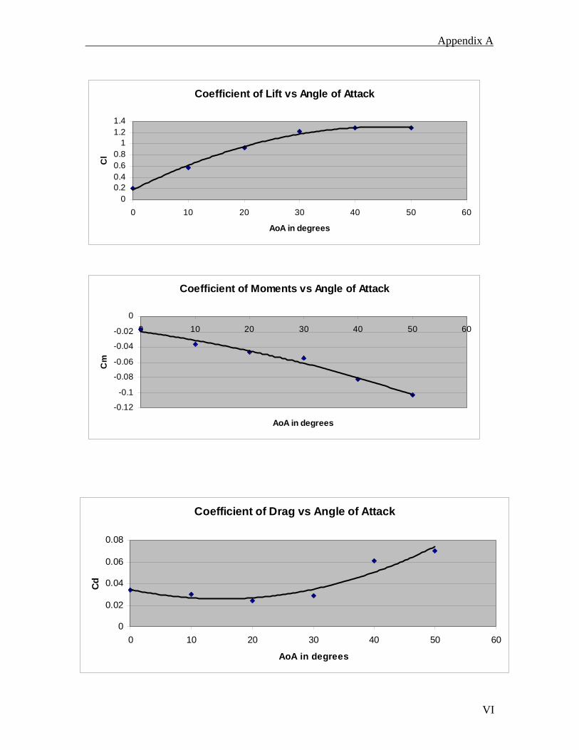
Appendix A

Coefficient of Lift vs Angle of Attack

00.20.40.60.8

11.21.4

0 10 20 30 40 50 6

AoA in degrees

Cl

0

Coefficient of Moments vs Angle of Attack

-0.12

-0.1

-0.08

-0.06

-0.04

-0.02

00 10 20 30 40 50

AoA in degrees

Cm

60

Coefficient of Drag vs Angle of Attack

0

0.02

0.04

0.06

0.08

0 10 20 30 40 50 6

AoA in degrees

Cd

0

VI

Appendix A

And finally the Lift and Drag Polar,

Graph of CL/CD vs Angle of Attack

0

10

20

30

40

50

0 5 10 15 20 25 30 35 40 45 50 55

AoA in degrees

CL/

CD

These curves represent the results of the reverse engineering procedure

and our understanding and increased knowledge of the Golden Eagle’s

airfoil, We see unique characteristics such as increased lift and reduced

drag at speeds of 10-20 m/s.

VII

Appendix B

Appendix B: Typical Airfoil Section Characteristics

Airfoil Section Characteristics Two dimensional properties only Reynold’s Number = 6,000,000

Lift coefficient values for l/d characteristics: .1, .4, .6

Drag Coefficient Values Airfoil

Shape Cl = .1 Cl = .4 Cl = .6

Max.

Cm.ac

L/d @

Cl = .1

L/d @

Cl = .4

L/d @

Cl = .6

Max.

Section Cl

0009 .0057 .0060 .0068 0.0 17.54 66.67 88.23 1.32

0010-34 .0043 .0065 .0076 0.0 23.26 61.53 78.94 .75

0012 .0058 .0066 .0076 0.0 17.24 60.61 78.94 1.59

1412 .0058 .0060 .0068 -.025 17.24 66.67 88.23 1.57

2412 .0065 .0061 .0071 -.04 15.38 65.57 84.50 1.69

4412 .0064 .0063 .0062 -.09 15.63 63.49 96.77 1.64

23012 .0061 .0063 .0065 -.013 16.39 63.49 92.31 1.76

63-212 .0045 .0045 .0063 -.035 22.22 88.89 95.24 1.58

63-412 .0056 .0048 .0052 -.075 17.85 83.33 115.38 1.73

63-415 .0052 .0052 .0055 -.07 19.23 76.92 109.09 1.64

64-412 .0059 .0046 .0051 -.073 16.94 86.96 117.64 1.67

64-415 .0052 .0050 .0051 -.07 19.23 80.00 117.64 1.60

64A212 .0046 .0045 .0072 -.04 21.74 88.89 83.33 1.50

64A215 .0045 .0048 .0071 -.037 22.22 83.33 84.50 1.50

65-212 .0040 .0051 .0072 -.035 25.0 78.43 83.33 1.46

65-412 .0055 .0042 .0053 -.07 18.18 95.23 113.21 1.61

65-415 .0046 .0042 .0045 -.068 21.74 95.23 133.33 1.58

VIII

Appendix B

66-212 .0033 .0056 .0076 -.03 30.30 71.43 78.94 1.45

66-415 .0057 .0039 .0042 -.074 17.54 102.56 142.85 1.57

747A315 .0050 .0044 .0048 -.012 20.00 90.90 125.00 1.36

747A415 .0063 .0044 .0048 -.03 15.87 90.90 125.00 1.42

GAW-2 .0072 .0055 .0070 -.10 13.89 72.73 85.71 2.04

NLF(1)-0215F .0074 .0064 .0046 -.13 13.51 62.50 130.40 1.72

NLF(1)-0416 .0063 .0058 .0053 -.10 15.87 68.96 113.21 1.87

LS(1)-0413 .0085 .0080 .0080 -.11 11.76 50.00 75.00 2.07

GA(PC)-1 .0073 .0073 .0072 -.045 13.70 54.79 83.33 1.80

The following are a sample of Harry Riblett’s sections for general aviation

GA30-312 .0060 .0060 .0070 -.055 16.67 66.67 85.71 1.59

GA30-315 .0065 .0070 .0075 -.055 15.38 57.14 80.00 1.67

GA30-412 .0065 .0065 .0070 -.07 15.38 61.53 85.71 1.70

GA30-415 .0070 .0070 .0075 -.07 14.28 57.14 80.00 1.80

GA35-312 .0060 .0055 .0060 -.055 16.67 72.72 100.00 1.58

GA35-315 .0060 .0060 .0065 -.055 16.67 66.67 92.30 1.70

GA35-412 .0070 .0055 .0060 -.072 14.28 72.72 100.00 1.65

GA35-415 .0060 .0060 .0065 -.073 16.67 66.67 92.30 1.82

GA37-312 .0060 .0055 .0055 -.06 16.67 72.72 109.09 1.54

IX

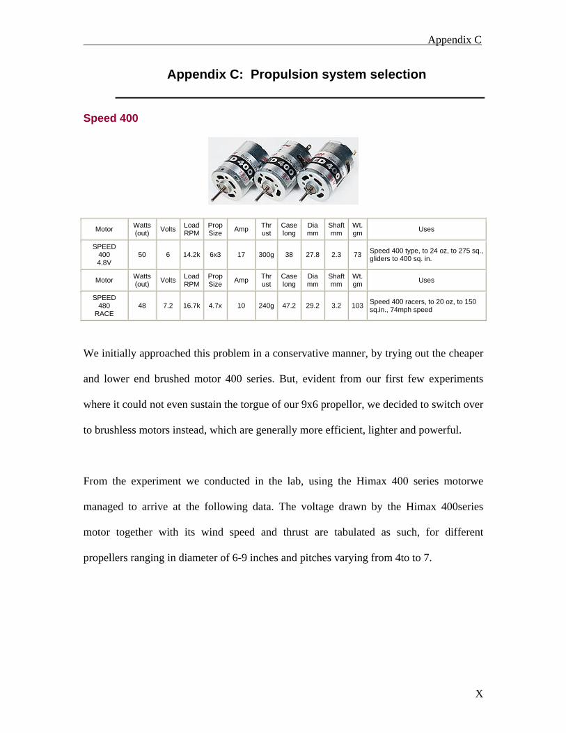
Appendix C

Appendix C: Propulsion system selection

Speed 400

Motor Watts (out) Volts Load

RPM Prop Size Amp Thr

ust Caselong

Diamm

Shaftmm

Wt.gm Uses

SPEED 400 4.8V

50 6 14.2k 6x3 17 300g 38 27.8 2.3 73 Speed 400 type, to 24 oz, to 275 sq., gliders to 400 sq. in.

Motor Watts (out) Volts Load

RPM Prop Size Amp Thr

ust Caselong

Diamm

Shaftmm

Wt.gm Uses

SPEED 480

RACE 48 7.2 16.7k 4.7x 10 240g 47.2 29.2 3.2 103 Speed 400 racers, to 20 oz, to 150

sq.in., 74mph speed

We initially approached this problem in a conservative manner, by trying out the cheaper

and lower end brushed motor 400 series. But, evident from our first few experiments

where it could not even sustain the torgue of our 9x6 propellor, we decided to switch over

to brushless motors instead, which are generally more efficient, lighter and powerful.

From the experiment we conducted in the lab, using the Himax 400 series motorwe

managed to arrive at the following data. The voltage drawn by the Himax 400series

motor together with its wind speed and thrust are tabulated as such, for different

propellers ranging in diameter of 6-9 inches and pitches varying from 4to to 7.

X

Appendix C

The airspeed, thrust force and voltage drawn data is tabulated,

Windspeed Motor Prop Idle Mid Max

9x6 6.2 15.8 17.4 8x7 3.7 9.1 15.9 8x4 3.2 7.9 14.2 7x5 3.7 10.3 14.4 H

imax

6x4 3.8 12.5 19.5

We also experimented and tabulated the characteristics of the GS-400 motor,

Weight (Kg) Voltage 9x6 0.712 0.739 0.930 1.045 11.44 11.00 8.32 7.03 8x7 0.729 0.743 0.924 0.991 11.06 10.77 9.02 7.27 8x4 0.727 0.754 0.944 1.049 11.16 10.80 9.10 7.28 7x5 0.730 0.762 0.912 0.973 10.96 10.68 9.15 7.26

GS

6x4 0.721 0.730 0.811 0.835 11.26 11.05 9.82 7.42

Weight (Kg) Voltage Motor Prop zero Idle Mid Max zero Idle Mid Max

9x6 0.716 0.752 0.949 1.067 11.44 11.12 8.39 7.10 8x7 0.729 0.753 0.935 1.020 11.06 10.89 9.12 7.35 8x4 0.729 0.765 0.946 1.056 11.18 10.97 9.27 7.39 7x5 0.733 0.771 0.914 0.985 10.96 10.74 9.21 7.31 H

imax

6x4 0.723 0.739 0.817 0.851 11.26 11.10 9.89 7.46

Motor Prop Windspeed

9x6 6.0 15.6

17.1

8x7 3.2 8.6 15.2

8x4 3.0 7.5 13.9

7x5 3.4 10.0 14.0

GS

6x4 3.3 11.9 18.6

We, had to compare, at least two top end motors to arrive at a fair decision. Requiring

with aero enthusiasts on our field research trips to aero modeling shops we discovered the

XI

Appendix C

GS motor. Unfortunately, technical specifications for this particular model was not

readily available, hence we relied purely on experimental data.

We found that the thrust specifications for the smaller sized propellers were insufficient

for both motor at all three thrust settings, but as the pitch and diameter increased, the

differences in performance became more divergent. Although both motors provided the

required thrust, the Himax motor displayed longer sustainability, in that it could run at

100% throttle setting for much longer. Furthermore the himax was also a lighter motor

and good option for our power plant.

Via performance matching is so that we optimized the performance of the propulsion

system with the 9x6 pusher propeller to give us maximum thrust.

Our motor of choice is the himax, series; we have displayed here its recommended usage

and specifications that we discovered.

Operation:

1. Himax Brushless motors require brushless sensor less speed controls. Failure to use a

brushless sensor less electronic speed control (ESC) can result in damage to the motor

and/or ESC. A Castle Creations Phoenix series ESC is recommended for best

XII

Appendix C

performance. The standard setting for timing advance is recommended for best

operation.

2. The three wires of the motor can be connected to the three output leads of the ESC in

any order. Check the direction of rotation of the motor. If the motor spins in the

wrong direction switching any two of the motor wires will reverse rotation. Be sure to

insulate the wires to prevent shorting which may damage the ESC.

3. Allow for proper cooling of the motor during operation. With extremely high capacity

batteries, care must be taken to prevent excessive motor temperature. Overheating of

the motor is not covered under warranty. Insufficient cooling can result in overheated

motors, even when operated at moderate power levels.

Features:

High Efficiency - High Power - Light-weight - Replacement for 500-600 Motors

Specifications:

Weight: 138g, (4.9oz), Motor Only

Max Power: 400W, (This is dependent on several factors)

Max RPM: 50,000 RPM

Diameter: 28mm, (1.10”)

Length: 36.8mm, (1.45”)

Shaft Diameter: 4.0mm, (.1575”) or 3.17mm (.125”)

Mounting Screw Thread: 3.0mm, max depth 4.0mm, on 16mm, (.625”) bolt circle

Maximum Case Temperature: 100oC, (212oF)

Electrical Specifications:

HA2825-2300 Kv = 2300, Rm = .078, Io = 0.5, Efficient Operating Current = 4-23A

XIII

Appendix C

Himax HA2015 series brushless motors - Speed 280/300 replacement

• Slotless design for high efficiency. High performance replacement for Speed 280/300

type can motors, • For light electric planes under 20oz or 3-D performance under 13oz, • Fit most slowflyer/parkflyers _ GWS planes, micro helicopters - Hummingbird & Piccolo,

micro cars - mini T & HPI micro,

Himax HA2025 series brushless motors - Speed 370/400/480 replacement

• Slotless design for high efficiency. High performance replacement for Speed 370/400/480 type can motors,

• For light electric planes under 30oz or 3-D performance under 18oz, • Perfect for 3-D aerobatic, pylon race, and any application maximum power/weight ratio

is needed,

Himax HA2825 series brushless motors

• Slotless design for high efficiency. High performance replacement for 500/550 type can

motor, • Gear motors are suitable for small electric trainers, sport fun flyers, • Direct drive motors are best for ducted fans & pylon racers where high rpm is a must, • For light electric planes under 70oz.
XIV
We are using the 3600 series motor, which displays current to voltage consumption as

such, comparing against this graph, we were able to, select the power supply of 4 cells to

drive the propulsion system.

Appendix D

Appendix D: Aerofoil concepts

Research of airfoils and planforms was conducted referencing several aerodynamics

texts. Two of these texts, the American Institute of Aeronautics and Astronautics (AIAA)

published Fixed and Flapping Wing Aerodynamics for Micro Air Vehicle Applications1

and their independently written Model Aircraft Aerodynamics by Martin Simons,

contained a substantial amount of material concerning low-speed airfoil research. From

these texts we researched several thin and thick airfoils.

Seperation bubble on low speed airfoils (Ref: AIAA, pg.135) Both texts stated that at low Reynolds numbers thin airfoils outperform thicker profiles. It

might seem as though a very porous surface would create a substantial amount of extra

drag. This is true for larger aircraft that fly at much higher Reynolds numbers. A smooth

surface is a much better aerodynamic body at these speeds. However, at low speeds a

smooth surface is not always the best choice. Low speed, laminar flows are prone to

producing separation bubbles along the upper surface of a wing within a Reynolds

XV

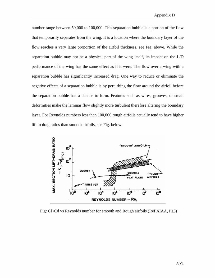
Appendix D

number range between 50,000 to 100,000. This separation bubble is a portion of the flow

that temporarily separates from the wing. It is a location where the boundary layer of the

flow reaches a very large proportion of the airfoil thickness, see Fig. above. While the

separation bubble may not be a physical part of the wing itself, its impact on the L/D

performance of the wing has the same effect as if it were. The flow over a wing with a

separation bubble has significantly increased drag. One way to reduce or eliminate the

negative effects of a separation bubble is by perturbing the flow around the airfoil before

the separation bubble has a chance to form. Features such as wires, grooves, or small

deformities make the laminar flow slightly more turbulent therefore altering the boundary

layer. For Reynolds numbers less than 100,000 rough airfoils actually tend to have higher

lift to drag ratios than smooth airfoils, see Fig. below

Fig: Cl /Cd vs Reynolds number for smooth and Rough airfoils (Ref AIAA, Pg5)

XVI

Appendix D

Sweep and Twist

Basic lift distribution consists of lifting root, downloaded tip -> positive Cm.

Camber distribution

An airfoil is defined by first drawing a “mean” camber line. The straight line that joins

the leading and trailing ends of the mean camber line is called the chord line. And the

length of this chord line is called chord,c. To the mean camber line, a thickness

distribution is added in a direction normal to the camber line to produce the final airfoil

shape. Equal amounts of thickness are added above the camber line, and below the

camber line. An airfoil with no camber (i.e. a flat straight line for camber) is a symmetric

XVII

Appendix D

airfoil. Whilst, that with appositive camber infront and a negative camber behind is

termed a reflexed airfoil.

Center of Pressure:

the center of pressure is defined as the point about which the pitching moment is zero. As

the flow conditions change (example, angle of attack α changes), the center of pressure

will change.

Aerodynamic Center: The aerodynamic pressure is defined as the point where the

pitching moment (or the pitching moment coefficient) is independent of α. That is, if we

computed the pitching moment about the aerodynamic center,

0=∂∂

=∂∂

ααmCM

XVIII

Appendix E

Appendix E: Weight and Balance Matching

One of the critical areas of conceptual design is that of weight and balance. As can be

imagined, the total weight of the vehicle will determine if it can fly or not,

but there are much more subtle aspects of weight and balance that play a vital role in the

conceptual design of an aircraft. The term “weight and balance” refers to the mass

properties of an aircraft and the resulting stability or lack thereof as a consequence of its

mass properties. The term mass properties usually includes the following values: volume

(or mass or weight), center of mass (or center of gravity), and the moments and products

of inertia. The weight of the vehicle is trivial to calculate, but can be the difference

between the success and failure of a mission. It is essential for calculating the residual

moments by way of derived equations from a “free body” diagram. A free body diagram

is used to visually sum all of the forces and moments on an object to determine its static

equilibrium or it’s dynamic response due to a particular loading.

The distribution of the vehicle’s weight is also of major concern. The locations of the

aircraft’s components and their corresponding weights will determine where the aircraft’s

center of gravity is located. The center of gravity (cg) is the point where the object’s

gravity force (or weight) acts. Also, it is around this point that the object naturally rotates

if a torque is applied. If a force is applied to an object and the force vector does not

intersect the CG, then a torque is also created about the CG proportional to the moment

arm(perpendicular distance from CG to the force vector).

XIX

Appendix E

In the case of aircraft, as it flies through the air, each of its components experiences

aerodynamic forces (not at the aircraft CG), thus creating torques about the CG. To

balance these torques, generally a control surface is deflected a certain amount to produce

a counter torque to nullify the overall moment felt at the CG. For this reason, the CG

location is critical for balancing the vehicle.

Finally, the moments and products of inertia (MOI )of the aircraft are also determined by

the distribution of the mass throughout the vehicle. Each component’s MOI and distance

from the aircraft CG affect the overall MOI. The MOI are used in dynamic analysis of the

aircraft and also to size the control surfaces. One example of a study where MOI are

critical would be to determine the dynamic response of the aircraft to a sudden gust of

wind.

The equations that command weight and balancing are,,

XX

Appendix E

These equations are a bit complex due to the integration involved in them. The c.g

equations can also be referred to as “first moment” equations. This is due to the fact that

each infinitesimal volume is multiplied by a moment arm. This moment arm adds the

concept of position of each particle into the equation. The process requires that the

moments (instead of masses) are summed, and then divided by the total volume. This is

like taking an average of all the positions of the points in an object. The final result is the

coordinates of the CG (or centroid).

The equations for moment of inertia, are also referred to as “second moment” equations.

This is due to the squared moment arm that multiplies each infinitesimal volume during

the integration. In the case of the Ixx

, the distance from the x-axis is the moment arm to be

squared, and due to the Pythagorean theorem, this squared distance is y2

+ z2. The same

method is used for the other moments of inertia.

XXI

Appendix E

The usefulness of this squared moment arm is derived from the fact that the amount of

time needed for a point mass at a particular radius to reach a given speed is proportional

to its mass and the square of the radius. The moments of inertia of an object can be

understood as its resistance to rotation (angular accelerations and decelerations).

By assuming a constant mass through out the different components we are analysing, we

can use the simplified estimation equations, ( Ref:Jon Roskam)

( ) ( )

( ) (

( ) ( )

( ) ( )

( ) ( )

( ) ( ) ∑

∑

∑

∑

∑

∑

=

=

=

=

=

=

=

=

=

=

=

=

−−=

=−−=

=−−=

−+−=

−+−=

++−=

ni

i

ni

i

ni

i

ni

i

ni

i

ni

i

XcgXiZcgZimiIzx

ZcgZiYcgYimiIyz

YcgYiXcgXimiIxy

YcgYiXcgXimiIzz

XcgXiZcgZimiIyy

ZcgZiYcgYimiIxx

1

22

1

22

1

22

1

22

1

22

1

22

0

0

)

The Component masses are found in AppendixG and the geometrical drawing and

solution follows below,

XXII

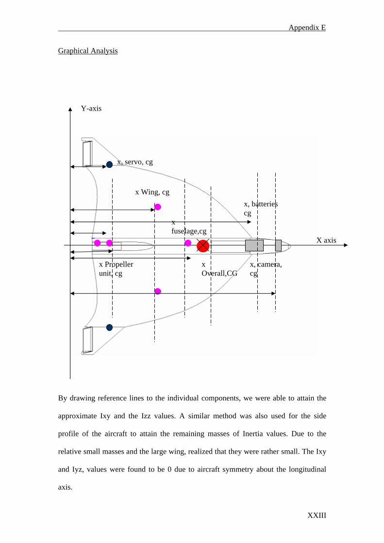
Appendix E

Graphical Analysis

X axis

x fuselage,cg

x Wing, cg

x Propeller unit, cg

x Overall,CG

x, batteries cg

x, camera, cg

Y-axis

x, servo, cg

By drawing reference lines to the individual components, we were able to attain the

approximate Ixy and the Izz values. A similar method was also used for the side

profile of the aircraft to attain the remaining masses of Inertia values. Due to the

relative small masses and the large wing, realized that they were rather small. The Ixy

and Iyz, values were found to be 0 due to aircraft symmetry about the longitudinal

axis.

XXIII

Appendix E

The Inertia tensor was,

⎪⎭

⎪⎬

⎫

⎪⎩

⎪⎨

⎧=

0.14663 0.02418- 0.01129- 0.02418- 0.13592 0.01718-

0.01129 - 0.01718- 07305.0

XXIV

Appendix F

Appendix F: Determining the Static Margin

Static margin is the distance between the C/G and the neutral point. If the C/G is

ahead of the neutral point, then the static margin is positive, and the static stability is

positive by an amount that is related to the static margin. If the C/G is behind the

neutral point, then the static margin and static stability are negative (i.e.: the model is

statically divergent, if you pull the nose up it wants to go up even more, shove the

nose down and it wants to tuck).

The well known Geometrical approximate method of determining the MAC is

illustrated for a Delta wing below,

XXV

Appendix F

MAC=

t m

Following the same procedure as for the MAC= 0.465m c.g ahead of AC = +0.0434m

Static Margin = % 33.9% 100465.0

0434.0=×

770m

delta w

of M

465mm

95mm
Mid-pt
Mid-p

ing we get,

AC

XXVI

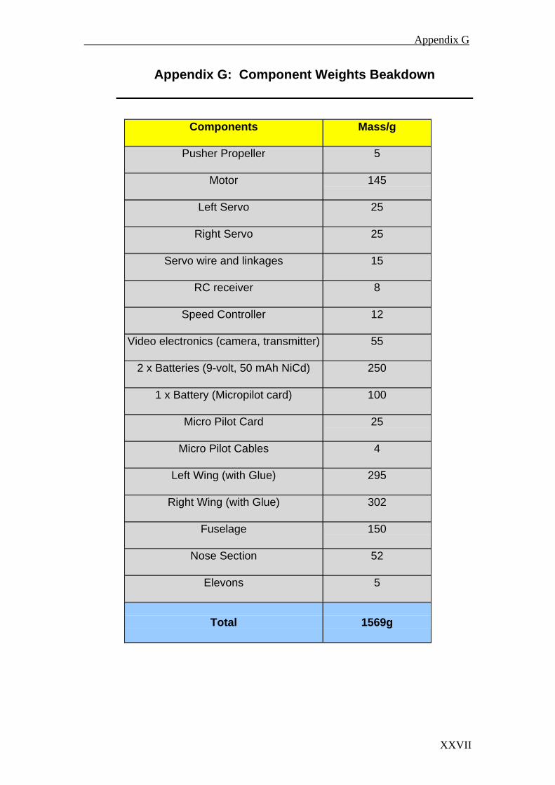
Appendix G

Appendix G: Component Weights Beakdown

Components Mass/g

Pusher Propeller 5

Motor 145

Left Servo 25

Right Servo 25

Servo wire and linkages 15

RC receiver 8

Speed Controller 12

Video electronics (camera, transmitter) 55

2 x Batteries (9-volt, 50 mAh NiCd) 250

1 x Battery (Micropilot card) 100

Micro Pilot Card 25

Micro Pilot Cables 4

Left Wing (with Glue) 295

Right Wing (with Glue) 302

Fuselage 150

Nose Section 52

Elevons 5

Total

1569g

XXVII

Appendix H

Appendix H: Camber Distribution of Airfoils

XXVIII

Appendix I

Appendix I: Benefits and Disadvantages of Flying Wings

2.4 Benefits and Disadvantages of the Flying Wing

The advantages of the Tailless Flying wing aircrafts are,

a) Fuselage and tail sections create extra drag reducing performance.

b) Reduced weight due to absence of tail components, (servos, rudder etc.)

c) Lower lateral radar visibility (flatter profile) due to absence of vertical tails.

d) Simple structure. Supposed to be easily made using composite materials

However, the following disadvantages also apply

a) Due to absence of vertical tail surfaces the aircraft experiences on its

longitudinal and vertical axes, relatively large inertia moments, while around its

transverse axis it is much smaller.

b) Aerodynamic damping of the rotation movements around its transverse axis is

less than that of conventional tailed aircrafts, leading to very sensitive and rapid

movement in this axis. (Hypersensitive aircraft)

c) Unstable and difficult to handle as control surfaces are relatively close to c.g.

(needs artificial stability resources – autopilot controls)

XXIX

abstract - national university of...

Documents