abstract - biomedical laser laboratory

Abstract

R. Scott Brock MODELING LIGHT SCATTERING FROM BIOLOGICAL CELLS

USING A FINITE-DIFFERENCE TIME DOMAIN METHOD. (Under the direction

of Dr. Jun Q. Lu) Department of Physics, January 2007.

The effect of cell morphology on light scattering is investigated using computer sim-

ulations. A parallel implementation of the finite-difference time domain (FDTD)

method has been developed to simulate the scattering and obtain various scattering

properties such as the Mueller matrix and anisotropy factor. In addition, a program

which produces 3D cell models for the FDTD program has been developed. Scatter-

ing from realistic red blood cell (RBC) and B-cell precursor (B-cell) models has been

simulated and the results are compared with those of the simpler sphere and coated

sphere models. The RBC models are based on models developed from mechanical

principles which impose constraints on the volume and surface area of an RBC under

pressure. The B-cell models are created by taking confocal microscopy images of

cultured NALM6 cells and applying statistical and geometric methods to produce a

realistic 3D model. Validation of the FDTD program against Mie theory results are

presented along with performance evaluations on three different parallel computing

platforms. Simulations of the more realistic cell models show that the sphere models

are not suitable for determining most of the scattering properties; however, a more

complex ellipsoid model provides a good approximation for some scattering proper-

ties. It was also found that the amount of forward scattered light is closely related

to the volume of the cell, while light scattered toward the side is more closely re-

lated to the refractive index. Simulations using various nucleus models show that the

complexity of the shape of the nucleus and its relative refractive index influence the

light scattering in various ways. A comparison with experimental results for cultured

NALM6 cells is also presented.

MODELING LIGHT SCATTERING FROM

BIOLOGICAL CELLS USING A

FINITE-DIFFERENCE TIME DOMAIN METHOD

A Dissertation

Presented to

the Faculty of the Department of Physics

East Carolina University

In Partial Fulfillment

of the Requirements for the Degree

Doctor of Philosophy in Biomedical Physics

by

R. Scott Brock

July 17, 2007

MODELING LIGHT SCATTERING FROM

BIOLOGICAL CELLS USING A

FINITE-DIFFERENCE TIME DOMAIN METHOD

by

R. Scott Brock

APPROVED BY:

DIRECTOR OF DISSERTATIONDr. Jun Q. Lu

COMMITTEE MEMBERDr. Xin-Hua Hu

COMMITTEE MEMBERDr. James M. Joyce

COMMITTEE MEMBERDr. Mark W. Sprague

COMMITTEE MEMBERDr. Mary A. Farwell

CHAIR OF THE DEPARTMENT OF PHYSICSDr. John C. Sutherland

DEAN OF THE GRADUATE SCHOOLDr. Patrick J. Pellicane

Dedicated to Ronald G. Hardy (1937–2006)

“Now he has departed from this strange world a little ahead of me. That

means nothing. People like us, who believe in physics, know that the dis-

tinction between past, present, and future is only a stubbornly persistent

illusion.” – A. Einstein

Acknowledgments

I would like to thank the faculty, staff, and graduate students of the Physics Depart-

ment for their help with my graduate studies. In addition, thanks go to the following:

Professor F. E. Bertrand and Dr. Douglas Weidner for providing the cells and confo-

cal images used in this study. Drs. Xin-Hua Hu and Huafeng Ding for providing the

experimental results. Dr. Ping Yang for providing a serial FDTD code. Mr. Maxim

Yurkin for some discussion which led to improvements in the FDTD code.

I would also like to acknowledge support through NIH grant 1R15GM70798-01

and various grants for computing resources from Teragrid.org, the San Diego Su-

percomputing Center, the North Carolina Supercomputing Center, the Pittsburgh

Supercomputing Center, and the Texas Advanced Computing Center.

Finally, I would like to thank Dr. Jun Q. Lu for her knowledge and patience

during my graduate studies, and in particular for her help and guidance with my

dissertation research.

Contents

List of Tables viii

List of Figures xi

INTRODUCTION 1

1 Introduction 1

THEORY 5

2 Scattering Theory 6

2.1 The model system . . . . . . . . . . . . . . . . . . . . . . . . . . . . . 6

2.2 The far field solution . . . . . . . . . . . . . . . . . . . . . . . . . . . 7

2.3 Scattered field properties . . . . . . . . . . . . . . . . . . . . . . . . . 9

METHODS 15

3 Near field methods 16

3.1 Finite-Difference Time Domain method . . . . . . . . . . . . . . . . . 16

3.2 Incident field . . . . . . . . . . . . . . . . . . . . . . . . . . . . . . . 21

3.3 Boundary condition . . . . . . . . . . . . . . . . . . . . . . . . . . . . 23

3.4 The discrete Fourier transform . . . . . . . . . . . . . . . . . . . . . . 26

3.5 Numerical dispersion . . . . . . . . . . . . . . . . . . . . . . . . . . . 27

4 Obtaining the scattered field properties 29

4.1 Scattering and Mueller matrices . . . . . . . . . . . . . . . . . . . . . 29

v

4.2 Cross sections and anisotropy factor . . . . . . . . . . . . . . . . . . . 30

5 Parallel methods 32

5.1 Near field . . . . . . . . . . . . . . . . . . . . . . . . . . . . . . . . . 33

5.2 Scattered field . . . . . . . . . . . . . . . . . . . . . . . . . . . . . . . 36

6 Cell model construction 38

6.1 General method . . . . . . . . . . . . . . . . . . . . . . . . . . . . . . 38

6.2 From analytic functions . . . . . . . . . . . . . . . . . . . . . . . . . 40

6.3 From domain images . . . . . . . . . . . . . . . . . . . . . . . . . . . 41

6.4 Visualization and volume calculation . . . . . . . . . . . . . . . . . . 43

RESULTS 47

7 Evaluation of the FDTD program 48

7.1 Overview . . . . . . . . . . . . . . . . . . . . . . . . . . . . . . . . . . 48

7.2 Program without the dispersion correction . . . . . . . . . . . . . . . 49

7.3 Dispersion corrected program . . . . . . . . . . . . . . . . . . . . . . 66

8 Red blood cells 73

8.1 The red blood cell . . . . . . . . . . . . . . . . . . . . . . . . . . . . . 73

8.2 The RBC model . . . . . . . . . . . . . . . . . . . . . . . . . . . . . . 73

8.3 The simulation results . . . . . . . . . . . . . . . . . . . . . . . . . . 74

9 NALM6 cells 88

9.1 Introduction . . . . . . . . . . . . . . . . . . . . . . . . . . . . . . . . 88

9.2 Image acquisition and processing . . . . . . . . . . . . . . . . . . . . 88

9.3 Validation of models constructed from confocal images . . . . . . . . 95

vi

9.4 Overview of the simulations . . . . . . . . . . . . . . . . . . . . . . . 99

9.5 Volume dependence . . . . . . . . . . . . . . . . . . . . . . . . . . . . 102

9.6 Comparison with an ellipsoidal model . . . . . . . . . . . . . . . . . . 113

9.7 Dependence on the nucleus and refractive index . . . . . . . . . . . . 115

9.8 Internal nuclear structure dependence . . . . . . . . . . . . . . . . . . 123

9.9 Comparison with experimental results . . . . . . . . . . . . . . . . . . 131

CONCLUSION 132

10 Conclusion 133

Bibliography 134

List of Tables

1 Qext by Mie theory and FDTD . . . . . . . . . . . . . . . . . . . . . . 58

2 g by Mie theory and FDTD . . . . . . . . . . . . . . . . . . . . . . . 58

3 Comparison of results with various number of PEs for a radii of 1.6µm

and 2.5µm . . . . . . . . . . . . . . . . . . . . . . . . . . . . . . . . . 58

4 Timing comparison for various problem sizes on the Lonestar cluster

for various problem sizes . . . . . . . . . . . . . . . . . . . . . . . . . 59

5 Timing comparison for various number of PEs on DSCC for a sphere

of radius 1.6µm . . . . . . . . . . . . . . . . . . . . . . . . . . . . . . 64

6 Timing comparison for various number of PEs on DSCC for a sphere

of radius 2.5µm . . . . . . . . . . . . . . . . . . . . . . . . . . . . . . 64

7 Timing comparison for various number of PEs on LSCC for a sphere

of radius 1.6µm . . . . . . . . . . . . . . . . . . . . . . . . . . . . . . 64

8 Timing comparison for various number of PEs on LSCC for a sphere

of radius 2.5µm . . . . . . . . . . . . . . . . . . . . . . . . . . . . . . 65

9 Timing comparison for various number of PEs on BLCC for a sphere

of radius 1.6µm . . . . . . . . . . . . . . . . . . . . . . . . . . . . . . 65

10 Timing comparison for various number of PEs on BLCC for a sphere

of radius 2.5µm . . . . . . . . . . . . . . . . . . . . . . . . . . . . . . 65

11 Errors in extinction cross section and anisotropy factor, resolution, and

time step information for the dispersion corrected validation tests. . . 67

12 Comparison of errors in extinction cross section with and without dis-

persion correction. . . . . . . . . . . . . . . . . . . . . . . . . . . . . 68

viii

13 Comparison of errors in anisotropy factor with and without dispersion

correction. . . . . . . . . . . . . . . . . . . . . . . . . . . . . . . . . . 68

14 Average cext and average g for 8, 12, and 20 incident angles . . . . . . 101

List of Figures

1 The model system . . . . . . . . . . . . . . . . . . . . . . . . . . . . . 7

2 The scattering plane . . . . . . . . . . . . . . . . . . . . . . . . . . . 10

3 The Yee cell . . . . . . . . . . . . . . . . . . . . . . . . . . . . . . . . 20

4 The total field/scattered field boundary . . . . . . . . . . . . . . . . . 21

5 The incident field projection . . . . . . . . . . . . . . . . . . . . . . . 23

6 The perfectly matching layer regions . . . . . . . . . . . . . . . . . . 25

7 Parallel grid division . . . . . . . . . . . . . . . . . . . . . . . . . . . 33

8 Parallel configuration of the time domain calculation for a cell. . . . . 34

9 The model cell . . . . . . . . . . . . . . . . . . . . . . . . . . . . . . 39

10 A domain image . . . . . . . . . . . . . . . . . . . . . . . . . . . . . . 41

11 A contour image . . . . . . . . . . . . . . . . . . . . . . . . . . . . . 42

12 Three dimensional model . . . . . . . . . . . . . . . . . . . . . . . . . 44

13 A marching tetrahedra cell . . . . . . . . . . . . . . . . . . . . . . . . 45

14 Tetrahedron facets . . . . . . . . . . . . . . . . . . . . . . . . . . . . 45

15 16 of the 256 possible facet combinations for a model cell, (a)before

and (b)after facet reduction. Associating facet groups with cells rather

than the individual tetrahedra simplifies processing. . . . . . . . . . . 47

16 Validation of Muller matrix for radius 1.6µm . . . . . . . . . . . . . . 50


18 Validation of Muller matrix for radius 3.75µm . . . . . . . . . . . . . 54



x


24 Red blood cell cross-sections for ∆P = 0, 1.2, 3, 10, 26 . . . . . . . . . 74

25 3D red blood cell models for ∆P = 0, 3, 10, 26 . . . . . . . . . . . . . 75

33 Set of confocal images for cell #8 . . . . . . . . . . . . . . . . . . . . 89

34 A confocal image for cell #8 . . . . . . . . . . . . . . . . . . . . . . . 90

35 Confocal image histogram . . . . . . . . . . . . . . . . . . . . . . . . 92

36 Processed confocal images . . . . . . . . . . . . . . . . . . . . . . . . 93

37 The confocal models for cell #s 1–10. The surfaces are transparent

allowing the model nucleus to be seen. The images are not on a par-

ticular scale; the smallest model, cell #1, has a volume of 445.46µm3,

while the largest, cell #9, has a volume of 737.33µm3. . . . . . . . . . 94

38 The confocal images for a 6µm diameter sphere. . . . . . . . . . . . . 96

39 The confocal sphere model from three different viewpoints. . . . . . . 96

40 A comparison of the scattering from a perfect sphere and the sphere

model obtained from confocal images. . . . . . . . . . . . . . . . . . . 97

41 Incident angles for the B-cell simulations . . . . . . . . . . . . . . . . 100

42 Confocal models vs. sphere models . . . . . . . . . . . . . . . . . . . 105



43 S11 results for cell #8. . . . . . . . . . . . . . . . . . . . . . . . . . . 108

44 S11 results for cell #10. . . . . . . . . . . . . . . . . . . . . . . . . . . 109

44 S12, S33, and S43 for the confocal model and sphere models of cell #8. 111

45 S11(θ = 0.25◦) vs. volume for the confocal models. . . . . . . . . . . . 112

46 Comparison of ellipsoids model and B-cell model . . . . . . . . . . . . 114

47 S11 for cell #8 with various refractive indices . . . . . . . . . . . . . . 115

xi

48 csca results for cell #8 with various refractive indices . . . . . . . . . 116

49 S12 for cell #8 with various refractive indices . . . . . . . . . . . . . . 117

50 S11, S12, and csca for cell #10. . . . . . . . . . . . . . . . . . . . . . . 120

51 Scatter plots of S11(θ = 0.25◦) vs. S11 integrated over other angles . . 122

52 Before and after of image filtered to remove high-frequency components 124

53 The functions determining the refractive index of the nucleus structure 126

54 Domain images of confocal models with nuclear structure. . . . . . . 127

55 The natural log and identity models . . . . . . . . . . . . . . . . . . . 128

56 S11, S12 for natural log and identity models . . . . . . . . . . . . . . . 128

57 S11, S12 for natural log models . . . . . . . . . . . . . . . . . . . . . . 128

58 Forward vs. 25◦ − 45◦ scattering for inhomogeneous nucleus models . 129

59 Comparison w/ experimental results, S11, S12 . . . . . . . . . . . . . . 131

Chapter 1: Introduction

Light scattering occurs when inhomogeneity exists in the path of incident light[2].

The scattering of light by small particles, i.e., particles with a size parameter com-

parable to the wavelength, is of great interest for a wide range of applications, such

as atmospheric scattering[46], scattering by interstellar gas clouds[12], and various

biomedical studies[19]. In the context of biomedical physics, it is widely recognized

that light scattering by a single cell of inhomogeneous body is very sensitive to its

morphology. Thus, the scattered light from a cell may provide a means for determin-

ing the characteristics of cell morphology.

Recent research activities in cell scattering have shown that different types of cells

can be associated with different scattering patterns. In 1998, the work of Mourant

et al. [30] showed that tumorigenic cells, M1 cells, and nontumorigenic cells, MR1

cells, have differences in scattering properties, and it was concluded that at least part

of this difference could be attributed to the difference in cell sizes. Drezek et al.

[14] combined numerical and experimental approaches in the study of both ovarian

cancer cells, OVCA-420 cells, and cervical cancer cells, He-La cells, and concluded

that the biochemical and morphological structure of the cells “strongly influenced”

the scattering properties. Other research results are related to the improvement of cell

modeling. Backman et al. [1] have used experimental data fitted to theoretical models

to show that scattered light measurements can be used to “give accurate quantitative

estimates” of the size distribution of cell nuclei and that “additional information” is

obtained about the refractive indices of cell organelles. In another recent report on cell

scattering measurements and data modeling, Mourant et al. [31] used three different

polarization configurations, i.e., parallel, perpendicular and cross polarization, when

measuring the angular distribution of the scattered light from epithelial cells and

2

isolated cell nuclei. With the aid of analytic models, i.e., Mie theory and T-matrix

method, that research provided useful information about refractive index structure

variations in epithelial cells and in isolated cell nuclei.

In order to maximize the potential of light scattering analysis as a tool for noninva-

sive probing of cell morphology, accurate modeling of light-cell interaction is needed.

However, light scattering from a biological cell is a complex phenomenon. In general,

biological cells are dielectric bodies with an inhomogeneous spatial distribution in

their refractive index. Thus, modeling the interaction requires the ability to account

for the inhomogeneous distributions. Also, biological cell size parameters range from

0.1 to 100, where the size parameter, x, is defined as x = 2πa/λ where 2a is the

characteristic dimension of the scatterer and λ is the wavelength of the incident light.

This size parameter range falls between the acceptable sizes for the Rayleigh approx-

imation (x� 1) and those of geometric optics (x� 1). This size range requires that

the modeling account for the wave nature of light and thus must be based on the

Maxwell equations.

In early studies, Mie theory has been used extensively to understand light scatter-

ing at the cellular level[2]. Mie theory provides an analytic solution to the problem

of light scattering by a homogeneous sphere. More recently, the anomalous diffrac-

tion approximation[39], multipole solutions[45], the T-matrix[32] method, the discrete

dipole approximation (DDA)[19, 20], and the finite-difference time domain method[41]

have been used to study cells with more realistic shapes. Although each of these

techniques offers some advantages over Mie theory, most require some geometric or

refractive-index contrast limitations that do not apply to the wide range of shapes

and refractive indices found in a cell. Mie theory and many implementations of

the T-matrix method require symmetries in the scattering particle. The anomalous

diffraction approximation used by Streekstra et al. [39] is restricted to a size parameter

3

x� 1 and a relative refractive index |m− 1| � 1. The multipole solutions of Videen

and Ngo [45] require effective medium substitutions for “more complicated systems

containing additional irregularities”[45], i.e., complex media must be replaced with

media having a single refractive index to approximate the net effect of the original

media.

From the research previously mentioned and other similar ongoing research, it is

clear that light scattering from biological cells is a complex phenomenon. The primary

goal of this research is to contribute to the understanding of this phenomenon and

obtain information that is pertinent to furthering research in biomedical optics.

One of the objectives contributing to this goal is producing a high-performance

numerical tool to model light interaction with biological cells. This tool is in the

form of a Fortran 90 implementation of the finite-difference time domain (FDTD)

method. The FDTD method has been chosen for this research due to the ability

to handle a wide range of scattering particles. The FDTD method does not require

symmetry in the scattering particles and can handle a wide range of refractive indices.

Alternatives to the FDTD method which have some of the same advantages as FDTD

are the DDA and the pseudo-spectral time domain method (PSTD). Like FDTD these

methods are not restricted to particles having particular symmetries. As mentioned

previously, the DDA has already been applied to scattering by biological cells[19, 20].

The PSTD method is similar to the FDTD method, but it also uses the spectral

components directly in the solution of the scattering problems. In addition to the

reasons already mentioned, FDTD was chosen because of the decades of development

of the method that had occurred prior to the start of this research and due to its

simplicity. The core of the FDTD method is finite differencing which is both easy

to understand and implement. The program has been developed using many of the

methods of the well-tested serial code developed by Yang and Liou [46] to study light

4

scattering by atmospheric ice crystals. The development process includes creating

the code, verifying results obtained, and evaluating the performance of the code.

Since the time required for the FDTD method increases cubically with the prob-

lem size and biological cells can have a size parameter as large as 100, it is practical

to use parallel computational methods to increase the amount of computational re-

sources that can be utilized simultaneously. As previous studies have shown[44, 11,

16, 26, 15, 21], parallel computational methods reduce the amount of time needed

to acquire results by allowing portions of the calculations to be carried out simul-

taneously. Parallel FDTD methods have been used previously on a wide variety of

platforms including shared-memory systems[7], massively parallel systems[34, 33, 18],

and workstation clusters[44]. In each of these cases, FDTD showed “excellent speed-

ups”[40]. The parallel implementation used in this research is a simplification of that

described by Taflove [40] and is discussed in detail in chapter 5. The communications

for the parallel program are implemented using the Message Passing Interface (MPI)

standard.

Another objective is to use the code to simulate the light scattering from biological

cells. To satisfy this objective, cell models must be created from information known

about the cells. In the case of the RBC, the analysis of Zarda et al. [49] of RBCs

under various pressure gradients has been used to create Fortran 90 code which will

generate RBC models. For the NALM6 cells, confocal images of NAML6 cells have

been obtained, and two other Fortran 90 codes have been written. One of these uses

the confocal images to obtain the data necessary to construct a cell model; the other

code uses the data obtained to construct the cell model.

The results of this research will contribute to the basic understanding of light

interaction with biological cells. In particular, results for scattering from RBCs[5, 25]

and NALM6[6, 13] cells has already been obtained. It provides not only these results,

5

but also the information about the performance and accuracy of an implementation

of the FDTD method. This will help other researchers in deciding which of the

many methods available is suitable for their light scattering research. In addition,

further understanding of light-cell interaction will contribute to research methods and

interests such as flow cytometry[4, 29], Monte-Carlo modeling of light[27, 10], and

possibly even to the diagnosis and treatment of illness or disease.

The remainder of this document is organized in four parts. The first part, chapter

2, contains a description of the physics theory necessary for this research. The second

part, chapters 3–6, describes the numerical methods used in this research. The third

part, chapters 7–9, presents the results of various numerical calculations which have

been carried out. The final part is the conclusion which summarizes the various parts.

Chapter 2: Scattering Theory

In general biological cells have size parameters ranging from 0.1 to 100. Thus, the

investigation of light scattering from these cells must consider the wave nature of

light. The fundamental equations describing this nature are the Maxwell equations.

Using the Maxwell equations, mathematical models are derived to describe the various

characteristics of the scattered light. Using these characteristics, comparisons can be

made between various particles to better understand the interaction between light and

biological cells. The first section of this chapter gives a description of the physical

system involved and the assumptions made about this system. Using this description,

an equation describing the scattered light is obtained. The second and final section

uses the equation derived to define properties of the scattered light which are useful

in analyzing the light-cell interaction. All of the definitions and derivations outlined

in this chapter are the result of previous work done in the field of electrodynamics

and are accepted practices in this field.

2.1 The model system

The system consists of an infinite homogeneous medium containing a scattering par-

ticle interacting with an electromagnetic field as shown in Fig. 1. By the superpo-

sitioning principle, the field, {E,H}, can be divided into two parts. The first is the

incident field, {Ei,Hi}, which is the field as it exists in the absence of the scattering

particle. The second is the scattered field, {Es,Hs}, which is the difference between

the existing field and the incident field, {E,H} − {Ei,Hi}. The incident field is a

plane wave with wavenumber vector ki. The infinite homogeneous medium, referred

to as the host medium, has permeability µ0 and permittivity ε0 and is non-absorbing,

7

(Ei,Hi)

(Es,Hs)

(ε0, µ0)

(ε, µ0)

ki

r

ks = |ki|r

r′

Figure 1: The model system consists of an electromagnetic field interacting with ascattering particle characterized by its permittivity, ε, embedded in a host mediumwith permittivity ε0. The incident field, {Ei,Hi}, is a plane wave with wavenumbervector ki. The scattered field, (Es,Hs), is unknown. The vectors ks, r, and r′ areshown for reference.

= (ε0) ,= (µ0) = 0. The scattering particle is non-permeable, µ = µ0, and is charac-

terized by its permittivity, ε. The scattered electric field, Es, is to be determined.

2.2 The far field solution

The Helmholtz equation for the electric field, E = Ei + Es, is

(∇2 + k2)

E (r) = −4πf (r)

f (r) =1

4π

(∇2 + k2)(ε (r)

ε0

− 1

)E (r)

, (2.1)

8

where k = |ki|. Applying the second Green identity with the free space Green’s

function, G, to Eq. (2.1); and using the fact that the scattered field vanishes at an

infinite distance, lim|r|→∞Es (r) = 0, yields

E (r) = Ei (r) +

∫V

f (r′)G (r, r′) d3r′

G (r, r′) =eik|r−r′|

4π|r− r′|, (2.2)

where V is the region occupied by the scattering particle. From Eq. (2.2) it is clear

that the second term on the right-hand side is the scattered field. In the far field, the

limiting form of G,

limkr→∞

G (r, r′) ∼ eikr

r, (2.3)

is used along with Eq. (2.2) to give the scattered field

Es (r) = F (ki,ks)eikr

r

F (ki,ks) =1

4π

∫V

(∇2 + k2)(ε (r′)

ε0

− 1

)E (r′) eiks·r′d3r′

. (2.4)

The arguments ks = kr and ki are explicitly shown to emphasize the dependence on

both the direction of the incident field and the direction of scattering. It has been

shown that the Helmholtz equation in a dielectric medium can be written[17]

(∇2 + k2)E = − (k2I +∇∇) · (( ε

ε0

− 1

)E

), (2.5)

where I is the unit dyad. Eq. (2.4) and (2.5) together yield

F (ki,ks) =k2

4π

∫V

((ε (r′)ε0

− 1

)E (r′)− rr · E (r′)

)eiks·r′d3r′ . (2.6)

9

From Eq. (2.4) and (2.6), it is clear that the scattered field is related to both the

shape of the scattering particle, V , and the distribution of the permittivity, ε (r′),

within the region of the scattering particle. Thus, particles which differ in either of

these properties will, in general, have scattered fields that also differ.

2.3 Scattered field properties

Using the model discussed in the previous section, the scattered field can be de-

termined when given an incident field, a host medium, and a scattering particle.

However, direct comparison of the scattered fields for different input factors is not

practical. Instead, several scattered field properties can be derived to which a physi-

cal meaning can be attached. Comparison of these properties allows a better analysis

of how the various input factors affect the light scattering. In particular, the Mueller

matrix, an angle dependent property, and the anisotropy factor and cross-sections,

scalar properties, are used to compare the results of various scattering simulations.

Calculation of the Mueller matrix begins by first calculating the scattering am-

plitude matrix, S. The scattering amplitude matrix gives a general relation between

the scattered field and a plane wave of arbitrary polarization. Using the geometry

shown in Fig. 2, this relationship is

Eα,s

Eβs,s

=eikr

r

S2 S3

S4 S1

Eα,iEβi,i

, (2.7)

where eα ⊥ eβs , eα × eβs = ks, eα ⊥ eβi , eα × eβi = ki, the 2 × 2 matrix is S,

Ei = Eα,ieα +Eβ,ieβi , and Es = Eα,seα +Eβ,seβs . Note that the relationship between

the scattered and incident fields is given in terms of components perpendicular and

10

xy

ki

ks

α

α

βs

βi

θ

φ

Figure 2: The scattering amplitude matrix is expressed in relation to the scatteringplane, shown in grey. θ and φ give the polar and azimuthal angles, respectively, of kswith respect to ki. The scattering plane is normal to (− sin (φ) , cos (φ)). {ex, ey, eki},{eα, eβi , eki}, and {eα, eβs , eks} are Cartesian basis sets for the various coordinatesystems used.

parallel to the scattering plane, thus allowing a 2× 2 matrix. Using the (eα, eβs , eks)

also simplifies Eq. (2.6) by eliminating the second term of the kernel, since α, β ⊥ r.

From the geometry, a matrix R can be defined

Eα,iEβi,i

= R

Ex,iEy,i

R =

βi · ex −βi · eyβi · ey βi · ex

=

cos (φ) − sin (φ)

sin (φ) cos (φ)

, (2.8)

which transforms vector components from the{

ex, ey, ki

}basis to the

{eα, eβi , ki

}

11

basis. Applying Eq. (2.8) to Eq. (2.7) gives

Eα,sEβ,s

=eikr

rS R

Ex,iEy,i

, (2.9)

where Ei = Ex,iex + Ey,iey. Notice that to find S, four equations are needed. Using

Eq. (2.6) will provide two equations, one for each element of F. Thus, Eq. (2.6)

must be used twice to get the necessary information, and each result for F must be

linearly independent. So, using Eq. (2.9) and Eq. (2.6), the relation between F and

S is determined by using two incident fields having orthogonal polarization vectors,

S =1

|Ei|

Fα∣∣Ei=Eiey Fα∣∣Ei=Eiex

Fβ∣∣Ei=Eiey

Fβ∣∣Ei=Eiex

R−1 , (2.10)

where F = Fαeα + Fβeβs , or using Eq. (2.6),

F (ki,ks) =k2

4πr

∫V

(ε (r′)ε0

− 1

)eα · E (r′)

eβ · E (r′)

eiks·r′d3r′. (2.11)

.

Although the scattering amplitude matrix gives the desired relation for an arbi-

trary polarization, it is more practical to use the Mueller matrix, M, to relate the

scattered and incident fields by their Stokes vectors. This relation is expressed as

Is

Qs

Us

Vs

=

S11 S12 S13 S14

S21 S22 S23 S24

S31 S32 S33 S34

S41 S42 S43 S44

Ii

Qi

Ui

Vi

, (2.12)

12

where the 4× 4 matrix is M; and I,Q, U, and V form the Stokes vector. One reason

this is more practical is that the Stokes vector components can be calculated di-

rectly from intensity measurements obtained experimentally. This allows for a direct

comparison with experimental results. Another reason is that several of the Mueller

matrix elements can be given a clear physical meaning. For example, S11 gives the

intensity of the scattered light. The components of M are related to the components

of S by

S11 =1

2

(|S1|2 + |S2|2 + |S3|2 + |S4|2)

S12 =1

2

(|S1|2 − |S2|2 + |S3|2 − |S4|2)

S13 = Re (S2S∗3 + S1S

∗4)

S14 = Im (S2S∗3 + S1S

∗4)

S21 =1

2

(|S2|2 − |S1|2 − |S4|2 + |S3|2)

S22 =1

2

(|S2|2 + |S1|2 − |S4|2 − |S3|2)

S23 = Re (S2S∗3 − S1S

∗4)

S24 = Im (S2S∗3 − S1S

∗4)

S31 = Re (S2S∗4 + S1S

∗3)

S32 = Re (S2S∗4 − S1S

∗3)

S33 = Re (S1S∗2 + S3S

∗4)

S34 = Im (S2S∗1 + S4S

∗3)

S41 = Im (S4S∗2 + S1S

∗3)

S42 = Im (S4S∗2 − S1S

∗3)

S43 = Im (S1S∗2 − S3S

∗4)

S44 = Re (S1S∗2 − S3S

∗4)

. (2.13)

13

Thus, once S is calculated, M is easily determined. As mentioned previously, the

Mueller matrix is the only angle dependent property used for comparing scattered

fields.

The anisotropy factor, g, is among the scalar properties that will be used for

comparisons. It is calculated from the S11 element of the Mueller matrix by

g =

∫ π2

0

∫ 2π

0S11(θ, φ) cos(θ)dφdθ∫ π

2

0

∫ 2π

0S11(θ, φ)dφdθ

. (2.14)

Since S11 represents intensity, g indicates where the energy is scattered on average. For

example, g = 1 indicates complete forward scattering; and g = −1 indicates complete

backward scattering. The anisotropy factor is useful not only for comparisons; it

can also be used in random walk simulations of photons as a parameter to select

a particular function from a family of phase functions, e.g., the Henyey-Greenstein

function.

The other scaler properties that will be used for comparison are the absorption,

extinction, and scattering cross sections; σa, σe, and σs, respectively. The first of

these, σa, can be derived from the Poynting theorem,

−∇ · s =∂u

∂t+ J · E , (2.15)

where u is the energy density, t is time, S is the Poynting vector, and J is the current

density. When applied to the system model in the frequency domain, this becomes

−∇ · s =iω

4πε0

(Re (ε) E · E∗ + H ·H∗) +Im (ε)ω

4πE · E∗ . (2.16)

According to the physical interpretation of the Poynting vector, taking the real part

of the left hand side of Eq. (2.16) and integrating over the volume gives the amount of

14

electromagnetic energy absorbed by the particle[46]. Carrying out this operation and

normalizing by the incident electromagnetic flux yields the absorption cross-section,

σa =k

ε0|Ei|2∫V

Im (ε (r)) |E (r)|2d3r . (2.17)

Thus, the absorption cross-section is related to the energy that is absorbed by the

scattering particle.

The extinction cross-section can be obtained from the optical theorem,

σe =4π

kIm (f) , (2.18)

where f is the normalized scattering amplitude in the forward direction, which for

the model system is

f =1

|Ei|2 F (θ = 0) . (2.19)

Applying Eq. (2.18) and (2.19) to the model system gives

σe =k

|Ei|2∫V

Im

([ε (r)

ε0

− 1

]E (r) · E∗i (r)

)d3r . (2.20)

The derivation of the optical theorem gives a clear meaning to σe; it is a measure of

the total energy scattered or absorbed by the particle[23].

Since, the extinction cross-section accounts for both scattering and absorption

and the absorption cross-section accounts for absorption, the scattering cross-section

is easily obtained by taking the difference in these quantities,

σs = σe − σa . (2.21)

It is related to how much energy is scattered by the particle.

15

The Mueller matrix along with the cross-sections and the anisotropy factor are

the collection of scattered field parameters that will be used to make comparisons

between different scattering particles.

Chapter 3: Near field methods

The previous chapter has described the theoretical framework for the investigation

of light scattering. To make use of this framework, numerical tools are used to

simulate the system described in §2.1. The simulation will take the parameters used

to describe the system and calculate the scattered field in the time domain. The first

four sections of this chapter describe the various methods used in the simulation. The

final section describes some of the numerical difficulties that arise through the use of

these methods.

3.1 Finite-Difference Time Domain method

The basis of the FDTD method is the replacement of continuous operators in the

Maxwell Equations by finite difference operators. This results in a set of six algebraic

equations which relate field components at finite points in space to neighboring field

components. Thus, a continuous wave propagating through space is simulated by a

numerical wave propagating through the grid of points.

The Maxwell equations for the model system of §2.1 are

∇ · E = 0 ∇× E = − 1

µ

∂

∂tH

∇ ·H = 0 ∇×H = ε∂

∂tE

. (3.1)

Working with complex numbers is computationally more expensive than working

with real numbers, so an equivalent expression to Ampere’s law without the use of the

complex permittivity will save computational resources. To obtain such an expression,

the method described by Yang and Liou is used[46]. This starts by casting Ampere’s

17

law to the source dependent form

∇×H =ε′

c

∂E

∂t+

4π

cσE , (3.2)

where ε′ is the effective real permittivity and σ is the effective real conductivity.

Assuming a harmonic time dependence and transforming both forms to the frequency

domain gives

∇×H =− ikεE

∇×H =− ik(ε′ + i

4π

kcσ

)E. (3.3)

By comparison it is clear that the two expressions are equivalent if ε = ε′ + i4πkcσ.

Letting εr = ε′, εi = 4πkcσ, and τ = kc εi

εr, Eq. (3.2) becomes

∇×H =εrc

(∂E

∂t+ τE

), (3.4)

an expression using all real numbers.

To obtain the finite difference expressions, the operator ∂∂t

must be replaced with

a finite difference operator. Again, methods previously reported are used[46]. First,

Eq. (3.4) is written in the equivalent form

∂ {eτtE}∂t

= eτtc

εr∇×H , (3.5)

Then, the finite difference operator for ∂∂t

in Eq. (3.4) is found by integrating over the

time interval [n∆t, (n+ 1)∆t] which yields

eτ(n+1)∆tE∣∣n+1− eτn∆tE

∣∣n

=

∫ (n+1)∆t

n∆t

eτtc

εr∇×Hdt

≈eτ(n+ 12)∆t

c∆t

εr∇×H

∣∣n+ 1

2

, (3.6)

18

where the subscript denotes the time step at which the field is evaluated, i.e., E∣∣n

=

E (t = n∆t). Thus E∣∣n+1

is described using only values known from previous times

steps by

E∣∣n+1≈ e−τn∆tE

∣∣n

+ e−τ∆t2c∆t

εr∇×H

∣∣n+ 1

2

. (3.7)

To obtain the finite difference operator corresponding to ∇, consider the operator

∂∂ri

acting on a vector A. This is approximated using a central difference as

∂

∂riA ≈ A

∣∣n+1−A

∣∣n

∆ri

, (3.8)

where ∆ri = ri∣∣n+1− ri

∣∣n. Using this central difference operator for the components

of ∇ gives a new vector finite difference operator, which applied to Eq. (3.7) gives

three algebraic equations. Assuming equal length intervals, ∆, for each operator, the

equation corresponding to the x-component of the electric field is

Ex

∣∣i,j,k,n

= e−τ∆t∣∣i,j,k

Ex∣∣i,j,k,n−1

+

(e−τ

∆t2

∆t

εr∆

)∣∣i,j,k

×(Hz

∣∣i,j+ 1

2,k,n− 1

2

−Hz

∣∣i,j− 1

2,k,n− 1

2

−Hy

∣∣i,j,k+ 1

2,n− 1

2

+Hy

∣∣i,j,k− 1

2,n− 1

2

) , (3.9)

where the subscripts i, j, and k indicate the position at which the field is evaluated,

i.e., H∣∣i,j,k,n

= H (x = i∆, y = j∆, z = k∆, t = n∆t).

Substituting the continuous operators∇ and ∂∂t

with the finite difference operators

19

for the curl equations of Eq. (3.1) results in the six algebraic equations

Ex

∣∣i,j,k,n


Ex∣∣i,j,k,n−1

+

(e−τ

∆t2

∆t

εr∆

)∣∣i,j,k

×(Hz

∣∣i,j+ 1

2,k,n− 1

2

−Hz

∣∣i,j− 1

2,k,n− 1

2

−Hy

∣∣i,j,k+ 1

2,n− 1

2

+Hy

∣∣i,j,k− 1

2,n− 1

2

)Ey

∣∣i,j,k,n


Ey∣∣i,j,k,n−1

+

(e−τ

∆t2

∆t

εr∆

)∣∣i,j,k

×(Hx

∣∣i,j,k+ 1

2,n− 1

2

−Hx

∣∣i,j,k− 1

2,n− 1

2

−Hz

∣∣i+ 1

2,j,k,n− 1

2

+Hz

∣∣i− 1

2,j,k,n− 1

2

)Ez

∣∣i,j,k,n


Ez∣∣i,j,k,n−1

+

(e−τ

∆t2

∆t

εr∆

)∣∣i,j,k

×(Hy

∣∣i+ 1

2,j,k,n− 1

2

−Hy

∣∣i− 1

2,j,k,n− 1

2

−Hx

∣∣i,j+ 1

2,k,n− 1

2

+Hx

∣∣i,j− 1

2,k,n− 1

2

)Hx

∣∣i,j,k,n


Hx

∣∣i,j,k,n−1

+

(e−τ

∆t2

∆t

εr∆

)∣∣i,j,k

×(Ey∣∣i,j,k+ 1

2,n− 1

2

− Ey∣∣i,j,k− 1

2,n− 1

2

− Ez∣∣i,j+ 1

2,k,n− 1

2

+ Ez∣∣i,j− 1

2,k,n− 1

2

)Hy

∣∣i,j,k,n


Hy

∣∣i,j,k,n−1

+

(e−τ

∆t2

∆t

εr∆

)∣∣i,j,k

×(Ez∣∣i+ 1

2,j,k,n− 1

2

− Ez∣∣i− 1

2,j,k,n− 1

2

− Ex∣∣i,j,k+ 1

2,n− 1

2

+ Ex∣∣i,j,k− 1

2,n− 1

2

)Hz

∣∣i,j,k,n


Hz

∣∣i,j,k,n−1

+

(e−τ

∆t2

∆t

εr∆

)∣∣i,j,k

×(Ex∣∣i,j+ 1

2,k,n− 1

2

− Ex∣∣i,j− 1

2,k,n− 1

2

− Ey∣∣i+ 1

2,j,k,n− 1

2

+ Ey∣∣i− 1

2,j,k,n− 1

2

)

. (3.10)

Note, that the electric field components at some time step, (n+ 1) ∆t, depend on

the values of the magnetic field components at one-half time step earlier,(n− 1

2

)∆t,

and vice versa. This choice of differencing operators allows all of the electric field

components at time t to be calculated, followed by the calculation of all of the mag-

netic field components at time t + 12∆t, and so on. Along with the appropriate field

component placement, discussed in the next paragraph, this avoids the need to solve

simultaneous equations at each time step, which is computationally expensive.

The grid on which Eq. (3.10) are applied is composed of Yee cells[47]. As shown

20

ExEy

Ez HxHy

Hz

∆

Figure 3: The grid cell used is known as the Yee cell[47]. Each electric field componentis offset from two magnetic field comonents by one half the distance across the cell(∆/2), and vice versa. This configuration avoids the necessity of solving simultaneousequations at each time step.

in Fig. 3, each grid cell contains one of each of the field components. Each electric

field component is offset from two magnetic field components by one half the cell

dimension and vice versa. This grid arrangement implicitly enforces the divergence

equations of Eq. (3.1)[40], and allows the calculations at each time step to be carried

out without the need to solve a set of simultaneous equations.

Using finite difference operators and the Maxwell equations, the basic FDTD

method has been derived. This allows the simulation of electromagnetic waves as

numerical waves on a grid. Using the method described, the electric field updates

are calculated followed by the magnetic field update, which is in turn followed by the

next electric field update, and so on. This process is referred to as time marching. In

the following sections, the problems of introducing the source field and terminating

21

the grid will be addressed.

3.2 Incident field

The incident field is introduced into the grid using the total field/scattered field for-

mulation (TF/SF). It is so named because using this formulation, the grid has two

regions; one containing the total field, and one containing the scattered field only, as

Outer cells, E = E− Ei

Inner cells, E = E + Ei

TF/SF boundary

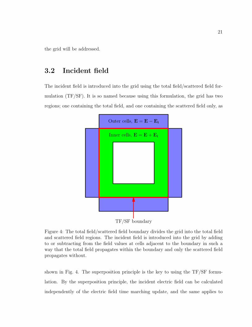
Figure 4: The total field/scattered field boundary divides the grid into the total fieldand scattered field regions. The incident field is introduced into the grid by addingto or subtracting from the field values at cells adjacent to the boundary in such away that the total field propagates within the boundary and only the scattered fieldpropagates without.

shown in Fig. 4. The superposition principle is the key to using the TF/SF formu-

lation. By the superposition principle, the incident electric field can be calculated

independently of the electric field time marching update, and the same applies to

22

the magnetic field. The sequence of field updates including the incident fields is (1)

update the electric field by time marching, (2) update the electric field using TF/SF

calculations, (3) update the magnetic field, and (4) update the magnetic field using

TF/SF calculations. This process is repeated until the simulation is complete.

To use the TF/SF method a boundary which surrounds the scattering particle

is chosen such that it lies on the surfaces shared by adjacent grid cells, as shown in

Fig. 4. At cells adjacent to this boundary, the known values of the incident field are

either added to or subtracted from the field components. The incident field is added

if the cell is within the boundary, and subtracted if it is not. This allows the normal

time stepping operations to propagate the incident field into the region of the particle,

while at the same time keeping the incident field confined to this region. Thus, two

regions can be identified, the one containing the scattering particle is the total field

region, and the other is the scattered field region.

Because the total field is being propagated numerically, numerical errors should be

included when calculating the incident field. For this reason, the incident field values

are also calculated numerically. This is accomplished by propagating the incident field

through an auxiliary one-dimensional grid, using a method similar to that of §3.1, and

projecting the field onto the three-dimensional grid at the TF/SF boundary. This

method is depicted in Fig. 5, where ki is the incident field direction, the cube is the

TF/SF boundary, the plane is the wavefront, and the red point and lines show where

the point is projected onto the boundary. This auxiliary grid method allows numerical

errors to be duplicated as the incident field propagates, thereby reducing the overall

error when adding the incident field values to the grid. Failure to duplicate the errors

would result in an unintended “error” wave propagating through the FDTD grid due

to the mismatch in values between the incident field in the auxiliary grid and the

FDTD grid. Because the incident field is a plane wave, known values can be added

23

TF/SF intersection

ki

Auxiliary grid intersection

Figure 5: The incident field is calculated in an auxiliary grid and projected onto theTF/SF boundary. The incident field is a plane wave with wavenumber vector ki. Thepoint at which the wavefront intersects the auxiliary grid and the points at which thewavefront intersects the TF/SF boundary all have the same field values.

to the cells at both ends of the auxiliary grid to stop the field propagation, just as

the TF/SF boundary does in the FDTD grid.

Using the methods of §3.1 and this section, an electromagnetic wave can be in-

troduced into a numerical grid which will simulate the interaction between the wave

and the scattering particle.

3.3 Boundary condition

In order to simulate the open space system on a finite grid, a technique called the per-

fectly matching layer absorbing boundary condition, or PML, is used. The particular

PML used in the simulation is called Berrenger’s PML, named after its developer[40].

24

The technique involves introducing a new (unphysical) medium which surrounds the

region of interest. This new medium is designed such that electromagnetic waves en-

countering the surface will be attenuated with minimal reflection. The new medium is

in turn, surrounded by a perfect electrical conductor, which will reflect the attenuated

waves back through the PML layer resulting in further attenuation before the wave

propagates back into the region of interest. This reduces the magnitude of the wave

by several orders of magnitude[40], making its contribution to the region of interest

negligible. To use this method, the FDTD Maxwell equations must be generalized by

separating each field component into two parts. For example, the Ex component is

split into the Eyx and Ez

x components according to whether the corresponding mag-

netic component differencing is in the x or y direction, respectively. This results in a

set of twelve equations to be used in the PML. Eq. (3.11) shows the FDTD equation

for Ex and the PML equations for Eyx and Ez

x for comparison.

Ex∣∣i,j,k,n


Ex∣∣i,j,k,n−1

+

(e−τ

∆t2

∆t

εr∆

)∣∣i,j,k

×(Hz

∣∣i,j+ 1

2,k,n− 1

2

−Hz

∣∣i,j− 1

2,k,n− 1

2

−Hy

∣∣i,j,k+ 1

2,n− 1

2

+Hy

∣∣i,j,k− 1

2,n− 1

2

)Eyx

∣∣i,j,k,n

= e−τy∆t∣∣i,j,k

Eyx

∣∣i,j,k,n−1

+

(e−τ

y ∆t2

∆t

εyr∆

)∣∣i,j,k

×(Hz

∣∣i,j+ 1

2,k,n− 1

2

−Hz

∣∣i,j− 1

2,k,n− 1

2

)Ezx

∣∣i,j,k,n

= e−τz∆t∣∣i,j,k

Ezx

∣∣i,j,k,n−1

+

(e−τ

z ∆t2

∆t

εzr∆

)∣∣i,j,k

×(Hy

∣∣i,j,k− 1

2,n− 1

2

−Hy

∣∣i,j,k+ 1

2,n− 1

2

)

. (3.11)

Notice that the permittivity, and the related τ , is not necessarily the same in all of

the equations. Similarly, the permeability of the PML is not necessarily that of the

host medium. This allows the contributions from finite differences over a direction

tangent to the PML surface to be attenuated, while those normal to the surface

25

are not, thereby reducing the reflection. Further, the permittivity and permeability

for the new medium are chosen so that the impedance is matched between the new

medium and the host medium,√

µε

=√

µ0

ε0, which means there will be no reflection for

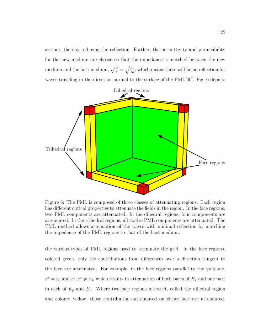
waves traveling in the direction normal to the surface of the PML[40]. Fig. 6 depicts

Trihedral regions

Dihedral regions

Face regions

Figure 6: The PML is composed of three classes of attenuating regions. Each regionhas different optical properties to attenuate the fields in the region. In the face regions,two PML components are attenuated. In the dihedral regions, four components areattenuated. In the trihedral regions, all twelve PML components are attenuated. ThePML method allows attenuation of the waves with minimal reflection by matchingthe impedence of the PML regions to that of the host medium.

the various types of PML regions used to terminate the grid. In the face regions,

colored green, only the contributions from differences over a direction tangent to

the face are attenuated. For example, in the face regions parallel to the yz-plane,

εx = ε0 and εy, εz 6= ε0, which results in attenuation of both parts of Ex and one part

in each of Ey and Ez. Where two face regions intersect, called the dihedral region

and colored yellow, those contributions attenuated on either face are attenuated.

26

Similarly, in the trihedral region, where three dihedral regions intersect and colored

red, all contributions are attenuated. Note that in Eq. (3.10), the permeability is not

present; however, using methods analogous to those of §3.1, the appropriate equations

can be derived with µ 6= µ0, which can be used to determine the PML equations for

the magnetic field components.

Through the use of the PML, outgoing waves can be attenuated twice (once af-

ter reflection) resulting in a negligible error wave propagating through the region of

interest. Thus, the physical open space model can be simulated numerically using a

grid of finite size. Combining this with the methods previously discussed, allows the

complete simulation of an incident electromagnetic field interacting with a scattering

particle in a homogeneous region of open space. During the simulation, the values of

the field components located within the scattering particle are calculated at each time

step. However, these field values are time domain values, and the needed values for

Eq. (2.6) are frequency domain values. The next section discusses the transformation

to the frequency domain.

3.4 The discrete Fourier transform

Using the procedures described so far, the near field in the time domain can be

determined over a discrete set of time steps; however, in order to calculate the desired

scattered field properties, the near field in the frequency domain is needed. This is

obtained by carrying out a discrete Fourier transform on all electric field components

located within the scattering particle according to

E (r, ω) ≈∑n

E (r, tn) eiωn∆t . (3.12)

27

According to Eq. (3.12), at each step of time marching a term for each component

is added, which results in the desired near field at the end of time marching. The

transform is also carried out on the incident wave at the center of the grid. At the

end of time marching, the total field is normalized by the incident field,

E =E′

|Ei| . (3.13)

where E′ denotes the field in the frequency domain. This allows for comparisons

which are independent of the magnitude of the incident field. All further references

to E refer to the normalized total field.

3.5 Numerical dispersion

The use of Eq. (3.10) causes the numerical wave to have certain numerical artifacts

as it propagates through the numerical space. Collectively, these effects are called

numerical dispersion. Numerical dispersion results in a phase velocity dependence on

wavelength, direction of propagation, and grid discretization. The dispersion relation

can be derived starting from a compact form of the Maxwell curl equations[40],

∇× (H + iE) =∂

∂t(H + iE) . (3.14)

Applying Eq. (3.14) to a monochromatic numerical plane wave,

(H0 + iE0) ei(kxi∆+kyj∆+kzk∆−ωt) , (3.15)

28

results in a set of three equations with three unknowns. Setting the determinant of

the system to zero results in

(∆

c∆t

)2

sin2

(1

2ω∆t

)= sin2

(1

2kx∆

)+ sin2

(1

2ky∆

)+ sin2

(1

2kz∆

), (3.16)

which is the dispersion relation. From Eq. (3.16), it is seen that ω = kc only in the

limit as ∆ goes to 0. Also, the velocity dependence on kx, ky, and kz indicates that

the grid, i.e., numerical space, is anisotropic.

One consequence of the numerical dispersion is that waves propagating in the

one-dimensional source grid, where ky, kz = 0, and the three-dimensional FDTD grid,

where generally kx 6= ky 6= kz, will have different velocities (except in the special

cases where the incident field travels parallel to a grid axis). This will cause an error

in introducing the source field to the grid due to the differing dispersion factors.

However, this error can be eliminated by deliberately changing the velocity of the

wave in the source grid. To do this, the wavenumbers for both grids are obtained

using Eq. (3.16) and the appropriate ratio of the wavenumbers is used to scale the

speed in the one-dimensional grid. This results in a wave traveling through the one-

dimensional grid at a velocity equal to that of the wave in the three-dimensional grid,

thereby aligning the wavefronts and eliminating errors due to differing velocities in

the projection operation described in §3.2.

Using the methods described in this chapter, the total electric field in the frequency

domain is obtained. This allows the calculation of F from Eq. (2.6). With this

information, all of the desired scattered field properties described in §2.3 can be

obtained. The next chapter describes how to calculate these values numerically.

Chapter 4: Obtaining the scattered field

properties

Using the result of the simulation described in the previous chapter, the various

scattering properties described in §2.3 can be calculated. This chapter describes how

the equations given in that section are treated numerically. The first section describes

the calculation of the matrix properties, while the second describes the calculation of

the scalar properties.

4.1 Scattering and Mueller matrices

With the total field in the frequency domain calculated, see §3, the scattering proper-

ties can be obtained. Since this is done numerically, the angular resolved quantities, S

and M, must be divided into discrete parts. A set of angles, azimuthal and polar with

respect to the scattering direction, is chosen with the desired resolution to quantify

these properties. This results in a discrete set of scattering wavenumber vectors, ksm,

where m denotes the mth vector of the set.

To calculate the scattering matrix, recall that Eq. (2.10) requires F to be calcu-

lated for two incident field polarizations. With the chosen set of scattering vectors

and using Eq. (2.10) and Eq. (2.4), the elements of S are calculated by replacing the

30

integral operation with a sum over the discrete volume elements. This yields

S2 (ksm) = i∆3 k3

4π

×∑n

(1− ε (rn))(eβ · ex α · E (rn)

∣∣Ei=ey

− eβ · ey α · E (rn)∣∣Ei=ex

)e−iksm·rn

S3 (ksm) = i∆3 k3

4π

×∑n

(1− ε (rn))(eβ · ey α · E (rn)

∣∣Ei=ey

+ eβ · ex α · E (rn)∣∣Ei=ex

)e−iksm·rn

S4 (ksm) = i∆3 k3

4π

×∑n

(1− ε (rn))(eβ · ex β · E (rn)

∣∣Ei=ey

− eβ · ey α · E (rn)∣∣Ei=ex

)e−iksm·rn

S1 (ksm) = i∆3 k3

4π

×∑n

(1− ε (rn))(eβ · ey β · E (rn)

∣∣Ei=ey

+ eβ · ex α · E (rn)∣∣Ei=ex

)e−iksm·rn

,

(4.1)

where rn denotes r at the center of the nth cell. Once S is obtained, M is calculated

taking the sum of the appropriate components of S according to Eq. (2.13). The final

result is a discrete set of numbers corresponding to the elements of M for the chosen

set of vectors ksm.

4.2 Cross sections and anisotropy factor

The anisotropy factor, g, is calculated by replacing the integral over the solid angle

with a sum over the scattering vectors, ksm. Applying this replacement to Eq. (2.14)

results in

g =

∑m S11 (ksm) ksm · ki∑

m S11 (ksm), (4.2)

where ksm · ki is the cosine of the polar angle.

31

Like S and g, the absorption and extinction cross sections from Eq. 2.17 and 2.20

are approximated by replacing the integral operation with a sum. For the absorption

cross section, the result comparable to Eq. (2.17) is

σa = k∆3∑n

Im (ε (rn)) |E (rn)|2 . (4.3)

Recall that the extinction cross section as derived from the optical extinction theorem

requires that only the scattering amplitude in the forward direction, ks0, be known.

The calculation analogous to Eq. (2.20) is

σe = k Im

(∑n

(1− ε (rn)) ep · E (rn)∣∣Ei=ep

e−iks0·rn), (4.4)

where the subscript p denotes the polarization. The use of ep is allowed by the electric

field having been normalized to the incident field, see Eq. (3.13). The scattering

cross section is calculated by taking the difference of the previously calculated cross

sections according to Eq. (2.21). Note that in general, the cross sections vary with

the polarization vector. When making comparisons of a particular cross section, the

average of the values for each polarization is used.

With the scattering properties calculated, comparisons between various scattering

systems can be compared. The Mueller matrix gives an angular resolved quantity for

comparison, while the cross sections and g allow comparison of scalar values.

Chapter 5: Parallel methods

Because the FDTD method models three-dimensional objects on a grid of points, the

number of spatial operations required grows with volume, and the number of temporal

operations grows with the distance that the incident field must travel. Thus, the

simulation time to obtain the near field is at least O(n3). The memory requirements

also depend on volume and are thus O(n3). For large scattering particles, this makes

it impractical or impossible to carry out simulations on single workstations. For this

reason, the program uses parallel methods, which allows simulations to be carried

out on a network of computers or multiple processor systems. Regardless of the

computing platform, a single processor and its associated memory will be referred to

as a processing element, or PE.

Many computing platforms are designed to handle calculations on values stored

contiguously in memory more efficiently than if they are stored non-contiguously. In

order to take advantage of these platforms, the field values are allocated in a con-

tinuous section of memory. This allows optimizations such as vectorizing algorithms

to be carried out by the compiler in order to produce efficient machine code. The

potential for such optimizations combined with the parallel methods, discussed in the

following sections, allows the program to run efficiently on a wide range of hardware,

from a single pc to a network of multi-processor supercomputers. However, to run

on a variety of platforms, the code must be written in a form that is portable. The

code is written in standard Fortran 90, with communications carried out by the Mes-

sage Passing Interface library (MPI). A Fortran 90 compiler and the MPI library are

available for most platforms.

Parallelizing the program can be divided into three stages. The first stage is to

parallelize the computation of the derivative parameters. This is accomplished by

33

communicating the initial parameters such as ki, λ, ε, etc., to all of the PEs, allowing

each PE to calculate any derivative parameters, e.g., ω, without the need for further

communications. Although this results in duplicate calculations on separate PEs,

the time taken is less than that used when calculating all derivative parameters on a

single PE and then communicating them. The other stages are parallelizing the near

field calculation, discussed in the next section, and parallelizing the calculation of the

scattered field properties, discussed in the final section.

5.1 Near field

PE

PE

PE

PE

PE

Cluster

z

Figure 7: The FDTD grid is divided into sections along planes perpendicular to thez-axis. Each processing element in the cluster is assigned one of these sections. Thisallows simulataneous computations of the field values for a single timestep.

The FDTD method of §3.1 is parallelized in a straightforward manner using a

simplified version of the method described by Taflove[40]. The computational space

34

Ex

Ey

Ez

Hz

Hy

Hx

Ex

Ey

Ez

Hz

Hy

Hx

Eswapx

Eswapy

Hswapy

Hswapx

tn

tntn+ 12

tn+ 12

Figure 8: Parallel configuration of the time domain calculation for a cell.

is divided along planes that are normal to the z-axis, as shown in Fig. 7. Each PE

can then calculate the field updates for a particular section of the grid. This division

leads to the additional burden of communicating boundary values at the edge of the

grid sections. For example, to calculate the x-component of the electric field at a

boundary normal to the z-axis, the y-component of the magnetic field calculated by a

neighboring PE is required. Conversely, the neighboring PE needs the x-component

of the electric field in order to calculate the y-component of the magnetic field. This

situation is illustrated in Fig. 8. Recall that the electric field updates and magnetic

field updates are separated in time. This allows the values to be exchanged as needed;

however, the space for the communicated values must be available in each of the PEs

in order to carry out the exchange. To do this, an extra layer of cells is added to each

z-normal face of a grid subsection. Because the grid is divided along a plane normal

to the z-axis, only four field values need to be communicated, specifically Ex, Ey, Hx,

and Hy. Since only the electric field is needed during the magnetic field update and

vice versa, the communication of two field values takes place at intervals of one-half

time step apart. The exchange illustrated in Fig. 8 depicts the grid division, the

35

communicated values, and the times at which the communications occur.

Because all PEs have a copy of the simulation parameters, the calculation of

the incident field can be done independently for each PE. As with the parameter

communication, this is more efficient than first calculating the incident field on one

PE and then communicating it. This also allows each PE to calculate the Fourier

transform of the incident field, see §3.4. The Fourier transform and normalization of

the total field is carried out by each PE only for the grid subsection on which that PE

operates. Thus, at the end of time marching, the total field in the frequency domain

remains distrubuted over the PEs in the same manner as the field in the time domain.

Although the using multiple PEs will reduce the overall time of the simulation and

reduce the memory required for each PE, there is a limit on how many PEs can be

efficiently used. This arises from the fact that the communication of boundary values

requires time. Typically, communicating a value takes more time than calculating

a value. So, as the number of PEs increases; the ratio of communication time to

computation time also increases, thereby reducing the efficiency of the simulation.

For example, assume adding PEs does not change the cpu time for computations

(t), i.e., the sum of the times for all PEs, or the total communication time (T ), i.e.,

simultaneous communication takes place. Then, the clock time (c) for a simulation

is c = t/n + T , where n is the number of PEs. Thus, the clock time asymptotically

approaches T with the number of PEs used. Thus, there is a point at which using

additional PEs no longer significantly reduces the clock time. Another consideration

in parallel simulations is load balancing, i.e., the distribution of operations across the

PEs. Suppose the grid is divided so that one PE has to perform more operations than

its neighbor, then the neighboring PE will have an idle period at each one-half time

step while it is waiting for the boundary values needed to begin the next step. The

FDTD program uses a load balancing method which divides the planes of grid cells

36

evenly along the z-axis; however, this does not divide the operations required evenly

since the PML and the Fourier transform calculations are not evenly distributed.

Generally, this results in less efficient load balancing as the number of PEs increases.

5.2 Scattered field

Unlike the FDTD method, parallelizing the calculation of the scattered field properties

requires only an initial communication followed by a few communications for some

of the desired properties. The initial communication occurs at the end of the time

marching process. This communication redistributes the near field values in the

frequency domain evenly among all of the PEs. The other communications will be

discussed in conjunction with their associated scattered field properties below.

The scattering amplitude matrix, S, is calculated in parallel by assigning each PE

to compute a portion of the sum in Eq. (4.1). Following this calculation, the results

of the partial sums are then communicated to a single process which takes the sum

of the communicated values. An equivalent form of Eq. (4.1) better represents this

process. For example,

S2 (ksm) = i∆3 k3

4π×∑m

∑n

(1− ε (rm,n))

×(eβ · ex α · E (rm,n)

∣∣Ei=ey

− eβ · ey α · E (rm,n)∣∣Ei=ex

)e−iksm·rm,n

, (5.1)

where m and n denote the nth element of the mth partial volume, is used to calculate

S2. Since the absorption and extinction cross sections each involve a similar volume

integral, the calculation of these cross sections are carried out in a comparable manner.

37

These are better represented by equivalent forms of Eq. (4.3) and (4.4).

σa =k∆3∑m

∑n

Im (ε (rm,n)) |E (rm,n)|2

σe =k Im

(∑m

∑n

(1− ε (rm,n)) ep · E (rm,n)∣∣Ei=ep

e−iks0·rm,n) , (5.2)

where again m and n denote the nth element of the mth partial volume.

Since the calculations associated with M, g, and σs, involve only algebraic oper-

ations over a small number of values, these are carried out by a single PE following

the parallel computations.

Chapter 6: Cell model construction

To use the program developed, models containing information about the index of

refraction of the scattering particle must be input into the program. To create the

models, the assumption is made that there is a finite number of refractive index values

which can be used to approximate the range of values found in the actual cells. For

example, a cell model may have two refractive index values; one corresponding to the

cytoplasm, and the other to the nucleus. Of course the model does not have to be

limited to two values, so complex models containing many values may be created.

The first section of this chapter describes the general method by which the models

are created. The second section describes how the general method can be applied

using analytic functions. The third section describes how more complicated models,

that may not be described analytically, can be created from raster data. The final

section describes how visualization and volume calculations can be carried on the

models obtained.

6.1 General method

According to Eq. (3.10), the permittivity must be known at the location of the field

components in the grid; so the model must contain at least this information. The Yee

cell, Fig. 3, can be divided into eight subcells as shown in Fig. 9. These subcells will

be referred to as model cells. Fig. 9 shows that each field component is at the corner

of eight model cells. Thus, if the permittivity is known at all corners of all model cells,

then the permittivity is known at all field component locations. The general method

for constructing a model is to create a function that given a location will return

the permittivity. This function will be called the model function. Using the model

39

ExEy

Ez

HxHy

Hz

Figure 9: For model construction the Yee cell is divided into eight subcells calledmodel cells. Each field component is located at the corner of eight model cells. Byobtaining the domains in which the corners of the model cells are located; the domainsin which the field components are located are also obtained. Knowing the domains ofthe model cells’ corners allows visualization via the marching tetrahedron algorithm.

40

function, the permittivity is obtained for the corners of all model cells. This method

allows the model generation program to be reused for various models with only the

requirement that a new type of model requires a new model function. Obtaining

information at the corners of all model cells, instead of just the field component

locations, allows visualization of the model using the marching squares or marching

tetrahedron algorithms.

6.2 From analytic functions

For analytic functions, the model function is simply a test against the implicit form

of the analytic function. For example, a homogeneous sphere of radius R has the

implicit function

x2 + y2 + z2 −R2 = 0,

and the model function is

f (x, y, z) =

ε , if x2 + y2 + z2 −R2 ≤ 0

ε0 , otherwise

.

Thus the model function returns ε if point (x, y, z) is within or on the sphere and

ε0 otherwise. The homogeneous sphere is a simple example; however, more complex

shapes follow exactly the same principle as long as they can be expressed analytically

with an implicit function.

41

6.3 From domain images

For shapes which cannot be described analytically, a “z-stack” of domain data may

be used. The z-stack of domain data is a set of images which are parallel to each

other and perpendicular to the z-axis. The data consists of pixels having colors, which

represent the domains. For example, Fig. 10 is an image containing data for three

Figure 10: A typical domain images. Three domains are represented by black, green,and yellow. The black domain is the background domain.

domains; one represented by black, another by green, and a third by yellow. In order

to construct the model function, the height and width of the pixels, and the distance

between images must also be known. In addition, the set relationship between the

domain data must be known, e.g., in Fig. 10 the yellow is a subset of the green and

the green is a subset of the black. It is assumed that a single domain is found along

the edges of each image, and this domain is referred to as the background domain.

With this information, a model function can be constructed.

To construct the model function, the non-background domains are considered

individually. To process a domain the boundary pixels of the domains in each image

42

are defined. This is done by removing the interior pixels of each image leaving only

a series of pixels which have exactly two neighboring pixels, as shown in Fig. 11.

Figure 11: The boundary pixels for the yellow and green domains of Fig. 10. Thecontour of the background domain is the image boundary, but it is not needed forthe model construction process.

Recall that the model function takes a locations, call it (x, y, z), as an argument. The

z-coordinate may or may not lie on one of the image planes, so define {zi} as the

ordered set of z-coordinates of the image planes such that zi+1 > zi. Now define a set

of piecewise linear contour functions,{Cjzi

}for each of the domains,

Cjk,zi

(t) = (xk, yk) +(xk+1, yk+1)− (xk, yk)

|(xk+1, yk+1)− (xk, yk)|t, 0 ≤ t ≤ 1, 1 ≤ k ≤ n, (6.1)

where Cjk,zi

is the kth segment of the contour associated with the jth domain in the

image at zi and n is the number of boundary pixels for the same domain and image.

Note that the contours are closed, so for kmax, kmax + 1 = 1 to complete the cycle.

43

Using Eq. (6.1) a distance function is defined,

d (x, y, zi) =

− inf

{min

(|(x, y)− Cjk,zi

(t)|) , 1 ≤ k ≤ n}

if (x, y) ∈domain,

inf{

min(|(x, y)− Cj

k,zi(t)|) , 1 ≤ k ≤ n

}otherwise

(6.2)

where there are n boundary pixels for the jth domain in the image at zi. Thus d is

equal in magnitude to the shortest distance to a contour and the sign of d indicates

whether the point is within the domain. Further, define zm and zn such that

zm = inf ({zi|z − zi > 0})

zn = inf ({zi|zi − z > 0}), (6.3)

i.e., the z-coordinates of the two slides closest to z. Using Eq. (6.2) and 6.3 the model

function, f is defined,

f (x, y, z) = Inner({ε|ε = gi (x, y, z) , i = 1, 2, . . . , l

})gi (x, y, z) =

εi , if d (x, y, zm) + (z − zm) d(x,y,zn)−d(x,y,zm)zn−zm ≤ 0

ε0 , otherwise

, (6.4)

where there are l domains, and Inner returns the element whose corresponding domain

is not a superset of any other element’s corresponding domain.

6.4 Visualization and volume calculation

Once the model is constructed, there is a domain value associated with each corner

of the model cells. Using these values, a surface can be created for visualization and

volume calculation purposes; for example, Fig. 12 depicts such a surface. Surfaces are

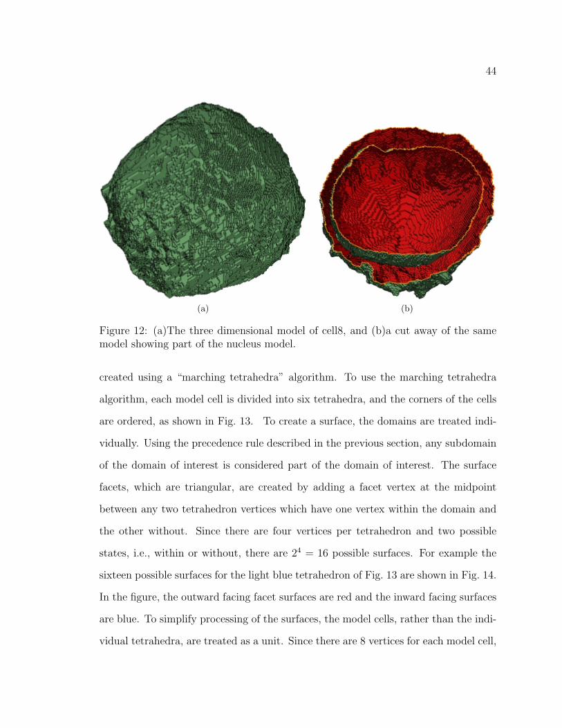
44

(a) (b)

Figure 12: (a)The three dimensional model of cell8, and (b)a cut away of the samemodel showing part of the nucleus model.

created using a “marching tetrahedra” algorithm. To use the marching tetrahedra

algorithm, each model cell is divided into six tetrahedra, and the corners of the cells

are ordered, as shown in Fig. 13. To create a surface, the domains are treated indi-

vidually. Using the precedence rule described in the previous section, any subdomain

of the domain of interest is considered part of the domain of interest. The surface

facets, which are triangular, are created by adding a facet vertex at the midpoint

between any two tetrahedron vertices which have one vertex within the domain and

the other without. Since there are four vertices per tetrahedron and two possible

states, i.e., within or without, there are 24 = 16 possible surfaces. For example the

sixteen possible surfaces for the light blue tetrahedron of Fig. 13 are shown in Fig. 14.

In the figure, the outward facing facet surfaces are red and the inward facing surfaces

are blue. To simplify processing of the surfaces, the model cells, rather than the indi-

vidual tetrahedra, are treated as a unit. Since there are 8 vertices for each model cell,

45

(a) (b)

Figure 13: (a)A model cell is divided into six tetrahedra. (b)The six tetrahedrashown individually. Model cells are divided this way for use in a marching tetrahedraalgorithm.

Figure 14: There are sixteen possible combinations of facets that can be associatedwith a tetrahedron according to which of the vertices are within the domain. Outwardfacing surfaces are marked red and inward facing surfaces, blue.

46

there are 28 = 256 possible groups of facets for any given cell. For each possibility,

the entire group of facets associated with the six tetrahedra of the cell are associated

with a unique integer ranging from 0 to 255. This is the reason for ordering the

corners of the model cells. By associating each corner with a binary bit, the integer

id is determined. For example a cell having corners 0, 3, and 7 within the domain

and the others without would have an id of 100010012 = 13710, where the subscript

denotes the base of the numbering system. To further simplify the processing, any

group of adjacent coplanar facets are replaced, if possible, by a group having the

minimum number of facets with the same perimeter. Fig. 15 shows sixteen of the

possible combinations both before (left) and after (right) facet reduction. Because

any two neighboring model cells share vertices, the facets associated with the cells

will necessarily share common edges, thereby creating a continuous surface, i.e., it is

not possible for there to be a “hole” in the surface due to mismatched vertices. By

adding facets to each model cell using this procedure, a surface which contains the

domain of interest is generated.

Visualization allows for checking the model against some expectation. Although

such checking is primarily subjective, it gives the opportunity to identify obvious

errors or flaws in the model construction process, e.g., an irregularity in a spherical

model or a large “bump” on a cell model which is not present in the confocal im-

ages. The stereolithography (STL) format is a standard used to represent surfaces

occupying three-dimensional space. It is a common format and there is a variety of

software allowing for visualization using this format. One of the requirements of the

STL format is that no vertex lie on an edge at any point other than an endpoint of

the edge, i.e., the endpoint of one edge does not lie between the endpoints of another

edge. For this reason, the surface construction process uses facets which conform to

this rule. This makes translating the surface to an STL format trivial.

47

(a) (b)

Figure 15: 16 of the 256 possible facet combinations for a model cell, (a)before and(b)after facet reduction. Associating facet groups with cells rather than the individualtetrahedra simplifies processing.

Another advantage of creating the surface is for volume calculation. Given a

surface made up of polygonal facets, the exact volume interior to the surface can be

calculated. Thus, considering the model as an approximation of a physical object

allows the volume of that object to be estimated. All cell model volumes discussed

in this work are calculated using the constructed surface as a boundary.

Chapter 7: Evaluation of the FDTD

program

7.1 Overview

To test the program a series of validation and evaluation simulations have been carried

out. Unless specified otherwise, all of the simulations for validation and evaluation

used a homogeneous sphere with a relative complex index of refraction of 1.0385 +

i1.6804× 10−5, a Gaussian pulse with 1µm wavelength in the host medium and pulse

width of 30 time steps, an 8 cell PML, 8 cells between the heterogeneous and scattered

field regions, a 5 cell scattered field region, and a grid resolution, λh∆

, of 30, where λh

is the wavelength in the host medium. All simulations used a number of time steps

equal to eight times the number needed for an incident pulse to travel across the total

field region. The homogeneous sphere was chosen for comparison with Mie theory in

the validation tests. The relative index of refraction was chosen to be equal to that

of cytoplasm in an extracellular fluid.

The FDTD program has been continuously updated and improved since the orig-

inal validated program was completed. Therefore, there are two sets of evaluation

and validation results, those based on the original program and those based on the

program at the time of this writing. Testing of the original program has been done on

the Datastar cluster (DSCC) at the San Diego supercomputing center, the Lonestar

Cray-Dell cluster (LSCC) at the Texas Advanced Computing Center at the University

of Texas and one of the Biomedical Laser Laboratory computing clusters (BLCC) at

East Carolina University. Tests on the DSCC were carried out on IBM P655 nodes

which have 1.5GHz IBM Power4 processors and are connected by a 2GHz switch.

49

The LSCC consists of nodes having dual 3.06GHz Intel Xeon processors which are

connected by a gigabit switch. The BMLL network consists of 8 nodes with Intel

Xeon 3.06 GHz processors connected by a gigabyte switch. Testing of the current

program has been done on the Lemieux computing cluster (PSCC) at the Pittsburgh

supercomputing center. The PSCC consists of Compaq Alpha nodes containing Al-

pha EV6.8 1 GHz processors connected by a Quadrics interconnection network. The

results are arranged so that the original validation and evaluation are presented first,

followed by the latest results.

7.2 Program without the dispersion correction

To validate the code, several simulations have been carried out for spherical particles

at various radii. The results of these simulations have been compared to Mie Theory,

which provides an analytic solution. As shown in Table 1 and Table 2, Qext and g

obtained using Mie theory are matched by the FDTD code. The maximum error for

Qext is 3.44%. The errors for g are better with the magnitude of the maximum error

begin 0.000998%. The FDTD results for the Mueller matrix elements S11, S12, S33,

and S43 have also been compared against the Mie theory results for spheres of the

same radii. These results are shown if Fig. 16–19. Notice that the errors in the FDTD

results are more pronounced in the larger scattering angles (> 160◦), but overall the

result is satisfactory.

With any parallel code, there can be a problem with task dependence. Task

dependence is present if the results for simulations having the same parameters are

different when run with a different numbers of PEs. To test for task dependence,

the simulation has been run several times with a different number of PEs for each

run. The Qext and g results are shown in Table 3 for a sphere of radius 1.6µm and

50

10−510−410−310−210−1100101102

S11

0 30 60 90 120 150 180Scattering angle (◦)

MieFDTD

(a)

−0.4

−0.2

0

0.2

0.4

Rel

ativ

eE

rror


(b)

−0.5

0

0.5

1

−S12/S

11


(c)

−0.8

−0.6

−0.4

−0.2

0

Abso

lute

Err

or


(d)

Figure 16: Comparison of (a)S11 and (c)S12/S11 obtained by Mie theory and FDTDfor a sphere of radius 1.6µm. (b),(d)The error between Mie theory and FDTD resultsfor S11 and S12/S11, respectively.

51

−0.9

−0.6

−0.30

0.3

0.6

0.9

S33/S

11


(e)

−0.6

−0.3

0

0.3

Abso

lute

Err

or


(f)

−0.5

0

0.5

S43/S

11


(g)

−0.3

−0.2

−0.1

0

0.1

Abso

lute

Err

or


(h)

Figure 16: Comparison of (e)S33/S11 and (g)S43/S11 obtained by Mie theory andFDTD for a sphere of radius 1.6µm. (f),(h)The error between Mie theory and FDTDresults for S33/S11 and S43/S11, respectively.

52

10−510−410−310−210−1100101102

S11


MieFDTD

(a)

−0.7

−0.2

0.3

0.8

Rel

ativ

eE

rror


(b)

−0.5

0

0.5

1

−S12/S

11


(c)

−2

−1

0

1

2

Abso

lute

Err

or


(d)


53

−0.9

−0.6

−0.30

0.3

0.6

0.9

S33/S

11


(e)

−0.5

−0.2

0.1

0.4

Abso

lute

Err

or


(f)

−0.4−0.2

00.20.40.60.8

S43/S

11


(g)

−0.2

0

0.2

0.4

Abso

lute

Err

or


(h)


54

10−510−410−310−210−1100101102103

S11


MieFDTD

(a)

−2

−1

0

1

2

Rel

ativ

eE

rror


(b)

−0.5

0

0.5

1

−S12/S

11


(c)

−0.5

−0.2

0.1

0.4

Abso

lute

Err

or


(d)


55

−0.9−0.6

−0.30

0.3

0.60.9

S33/S

11


(e)

−0.7

−0.3

0.1

0.5

Abso

lute

Err

or


(f)

−0.5

0

0.5

1

S43/S

11


(g)

−2

−1

0

1

Abso

lute

Err

or


(h)

Figure 18: Comparison of (e)S33/S11 and (g)S43/S11 obtained by Mie theory andFDTD for a sphere of radius 3.75µm. (f),(h)The error between Mie theory andFDTD results for S33/S11 and S43/S11, respectively.

56

10−510−410−310−210−1100101102103

S11


MieFDTD

(a)

−5

−3

−1

1

Rel

ativ

eE

rror


(b)

−0.5

0

0.5

1

−S12/S

11


(c)

−0.3

0

0.3

0.6

0.9

Abso

lute

Err

or


(d)


57

−0.9

−0.6

−0.30

0.3

0.6

0.9

S33/S

11


(e)

−0.5

−0.1

0.3

0.7

Abso

lute

Err

or


(f)

−0.5

0

0.5

S43/S

11


(g)

−0.9

−0.6

−0.3

0

0.3

Abso

lute

Err

or


(h)


58

Table 1: Comparison of Mie theory and FDTD extinction efficiency results for asphere of various radii

Radius Mie theory FDTD Error (%)1.6 0.525195 0.515006 1.942.5 1.18466 1.16196 1.923.75 2.21194 2.15920 2.385. 2.99977 2.89645 3.44

Table 2: Comparison of Mie theory and FDTD anisotropy factor results for a sphereof various radii

Radius Mie theory FD-TD Error (%)1.6 0.981587 0.981685 -0.0009982.5 0.990478 0.990538 -0.0006063.75 0.994196 0.994194 0.00002015. 0.995327 0.995250 0.000774

are identical. In fact, all of the scalar properties and matrix elements obtained were

identical except those which have an actual value of zero. For the zero values, the

computed values were all less than 10−14, although the computed values do not agree

for simulations having a different number of PEs.

Table 3: Comparison of results with various number of PEs for a radii of 1.6µm and2.5µm

r = 1.6µm r = 2.5µm#PEs Qext g Qext g

Mie theory 0.525195 0.981587 1.18466 0.9904781 0.515006 0.981685 1.16196 0.9905382 0.515006 0.981685 1.16196 0.9905384 0.515006 0.981685 1.16196 0.9905388 0.515006 0.981685 1.16196 0.99053816 0.515006 0.981685 1.16196 0.99053832 0.515006 0.981685 1.16196 0.99053864 0.515006 0.981685 1.16196 0.990538

Performance is a critical issue for the simulation. It is the primary reason that the

parallel code has been developed. Table 4 shows the timing results for simulations of

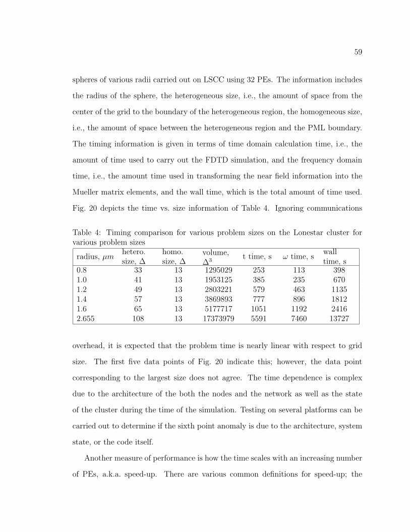
59

spheres of various radii carried out on LSCC using 32 PEs. The information includes

the radius of the sphere, the heterogeneous size, i.e., the amount of space from the

center of the grid to the boundary of the heterogeneous region, the homogeneous size,

i.e., the amount of space between the heterogeneous region and the PML boundary.

The timing information is given in terms of time domain calculation time, i.e., the

amount of time used to carry out the FDTD simulation, and the frequency domain

time, i.e., the amount time used in transforming the near field information into the

Mueller matrix elements, and the wall time, which is the total amount of time used.

Fig. 20 depicts the time vs. size information of Table 4. Ignoring communications

Table 4: Timing comparison for various problem sizes on the Lonestar cluster forvarious problem sizes

radius, µmhetero.size, ∆

homo.size, ∆

volume,∆3

t time, s ω time, swalltime, s

0.8 33 13 1295029 253 113 3981.0 41 13 1953125 385 235 6701.2 49 13 2803221 579 463 11351.4 57 13 3869893 777 896 18121.6 65 13 5177717 1051 1192 24162.655 108 13 17373979 5591 7460 13727

overhead, it is expected that the problem time is nearly linear with respect to grid

size. The first five data points of Fig. 20 indicate this; however, the data point

corresponding to the largest size does not agree. The time dependence is complex

due to the architecture of the both the nodes and the network as well as the state

of the cluster during the time of the simulation. Testing on several platforms can be

carried out to determine if the sixth point anomaly is due to the architecture, system

state, or the code itself.

Another measure of performance is how the time scales with an increasing number

of PEs, a.k.a. speed-up. There are various common definitions for speed-up; the

60

0

5000

1×104

1.5×104T

ime

(s)

0 5×106 1×107 1.5×107 2×107

Volume (∆3)

Time domainFrequency domain

Total

Figure 20: Timing results for spheres of various radii.

simplest of which is used here. Speed-up is defined as the ratio of the time used

by 1 PE to that used by x number of PEs; thus, the ideal speed-up for x PEs is x.

Simulations have been carried out on the three platforms mentioned to determine the

speed-up of the code. Fig. 21 depicts the timing information and the speed-up and the

ideal speed-up for simulations of two spheres, one (left) having a radius of 1.6µm and

the other having a radius of 2.5µm. From the figures, it can be seen that an almost

ideal speed-up is achieved on DSCC, while LSCC and BLCC show a similar less than

ideal speed-up. It should be noted that the ideal speed-up can not be achieved due to

communications overhead, and in fact, the performance will degrade as the number of

PEs is increased. This is due to the dependence communications time on the number

of PEs. The speed-up obtained on each of these clusters is more than satisfactory

to carry out the biological cell simulations. Tables 5–10 give the numerical data for

Fig. 21 and are included for reference.

61

0

5000

1×104

1.5×104

2×104

Tim

e(s

)

0 25 50 75 100Number of PEs

Time domainFrequency domain

TotalSpeed-upIdeal speed-up

0

25

50

75

100

Speed

-up

(a)

0

1.75×104

3.5×104

5.25×104

7×104

Tim

e(s

)


0

25

50

75

100

Speed

-up

(b)

Figure 21: Speed-up on DSCC for (a)r = 1.6µm, (b)r = 2.5µm

62

0

7500

1.5×104

2.25×104

3×104

Tim

e(s

)


0

25

50

75

100

Speed

-up

(c)

0

1.5×104

3×104

4.5×104

6×104

Tim

e(s

)


0

25

50

75

100

Speed

-up

(d)

Figure 21: Speed-up on LSCC for (c)r = 1.6µm, (d)r = 2.5µm

63

0

5000

1×104

1.5×104

2×104

Tim

e(s

)


0

5

10

15

20

Speed

-up

(e)

0

1.75×104

3.5×104

5.25×104

7×104

Tim

e(s

)


0

5

10

15

20

Speed

-up

(f)

Figure 21: Speed-up on BLCC for (e)r = 1.6µm, (f)r = 2.5µm

64

Table 5: Timing comparison for various number of PEs on DSCC for a sphere ofradius 1.6µm

#PEs t time, s ω time, s wall time, s speed-up1 6677 7754 14470 1.002 3940 4017 7980 1.814 1959 2303 4276 3.388 994 1093 2097 6.9016 471 499 980 14.832 198 254 462 31.364 87 134 231 62.696 64 97 170 85.1

Table 6: Timing comparison for various number of PEs on DSCC for a sphere ofradius 2.5µm


Table 7: Timing comparison for various number of PEs on LSCC for a sphere ofradius 1.6µm


65

Table 8: Timing comparison for various number of PEs on LSCC for a sphere ofradius 2.5µm

#PEs t time, s ω time, s wall time, s speed-up2 18379 31669 50108 1.644 9289 15503 24832 3.318 4802 7829 12661 6.4916 2404 3904 6341 13.032 1245 1974 3257 25.264 651 992 1685 48.896 543 675 1269 64.8

Table 9: Timing comparison for various number of PEs on BLCC for a sphere ofradius 1.6µm

#PEs t time, s ω time, s wall time, s speed-up1 6056 12873 19082 1.002 5273 6614 12080 1.584 2809 3305 6293 3.038 1517 1775 3467 5.5016 815 818 1813 10.53

Table 10: Timing comparison for various number of PEs on BLCC for a sphere ofradius 2.5µm

#PEs t time, s ω time, s wall time, s speed-up1 21598 47783 69775 1.002 17950 24503 42886 1.634 10471 12932 24405 2.868 5443 6450 12819 5.4416 2949 3097 6489 10.8

66

7.3 Dispersion corrected program

A series of validation tests have been carried out for an updated program using the

dispersion correction described in §3.5. These tests were carried out for comparison

with DDA method[48]. This series of tests required that the error for the extinction

cross section be less than 1% and that the root mean square relative error in S11

be less than 25%. This differs from the tests of the previous sections which fixed

λ/∆ and the number of time steps. Thus, these new tests give the smallest λ/∆

and number of time steps which conform to the criteria. The range of the relative

refractive index, m, was between 1.02 and 2 and the size parameters s range from

10 to 100 (although not all combinations were tested). Table 11 summarizes the test

results. The parentheses appearing around a result indicate that the test criteria

were not met for that result. Note that all but three tests were able to meet the

criteria, and that the non-conforming results are still satisfactory when considering

the purpose of the simulation.

Also, two tests have been carried out for comparison with the validation results

of the previous section. The parameters of these tests are the same as those of the

previous section for r = 1.6, 2.5; with the exceptions that the number of times steps

is equal to three times that required for the incident wave to travel across the het-

erogeneous region (eight times in previous), and that the heterogeneous space is two

grid cells thick (thirteen grid cells in previous). Table 12 and Table 13 show the

extinction cross section and anisotropy factor for both the dispersion corrected and

non-dispersion corrected programs. The errors are reduced by an order of magnitude

for Qext and increase for g, but note that the error for g remains small (≈ 0.01%).

Fig. 22 and Fig. 23 show the Mueller matrix elements resulting from both programs.

Again, the dispersion corrected result is clearly better than those without the disper-

67

Table 11: Errors in extinction cross section and anisotropy factor, resolution, andtime step information for the dispersion corrected validation tests.

m s RE Qext RMS RE S11 λ/∆ time steps1.02 10 4.3×10−3 0.17 12 275. 20 9.3×10−4 0.22 14 509. 30 7.9×10−3 0.22 13 651. 40 3.3×10−3 0.21 22 1398. 60 5.9×10−3 0.20 32 4004. 80 4.3×10−3 (0.33) 32 5239. 100 . .

1.08 10 5.5×10−3 0.064 18 453. 20 1.0×10−2 0.063 19 1005. 30 9.3×10−3 0.054 19 2531. 40 9.5×10−3 0.053 10 1928. 60 8.3×10−3 0.072 18 2509. 80 3.8×10−3 0.071 22 4009

1.2 10 7.6×10−3 0.024 18 671. 20 9.3×10−3 0.037 20 1589. 30 2.5×10−3 0.075 24 3321. 40 9.1×10−3 0.25 18 3837. 60 6.0×10−3 0.25 25 13762

1.4 10 8.9×10−3 0.14 10 1047. 20 9.8×10−3 0.17 37 10333. 30 8.2×10−3 0.19 23 11013. 40 (1.5×10−2) 0.24 32 21580

1.7 10 8.0×10−3 0.22 8 2323. 20 8.0×10−3 0.24 18 13101. 30 1.1×10−2 0.12 30 39751

2. 10 8.3×10−3 0.16 11 7481. 20 8.3×10−3 0.14 20 30693

68

sion correction.

Table 12: Comparison of errors in extinction cross section with and without dispersioncorrection.

radius Mie theory Qext w/ Error w/ (%) Qext w/o error w/o (%)1.6 0.525195 0.524461 0.14 0.515006 1.942.5 1.18466 1.18329 0.11 1.16196 1.92

Table 13: Comparison of errors in anisotropy factor with and without dispersioncorrection.

radius Mie theory g w/ Error w/ (%) g w/o error w/o (%)1.6 0.981587 0.981702 -1.17×10−2 0.981685 -9.98×10−4

2.5 0.990478 0.990577 -9.97×10−3 0.990538 -6.06×10−4

69

10−5

10−4

10−3

10−2

10−1

100

101

102

103

S11

0 45 90 135 180Scattering angle (◦)

Coated Sphere

w/o correction

w/ correction

(a)

−0.3

−0.125

0.05

0.225

0.4

Rel

ativ

eer

ror


(b)

−1

−0.5

0

0.5

1

S12


(c)

−0.7

−0.5

−0.3

−0.1

0.1

Abso

lute

erro

r


(d)


70

−1

−0.5

0

0.5

1

S33


(e)

−0.6

−0.375

−0.15

0.075

0.3

Abso

lute

erro

r


(f)

−1

−0.5

0

0.5

1

S43


(g)

−0.2

−0.125

−0.05

0.025

0.1

Abso

lute

erro

r


(h)


71

10−610−510−410−310−210−1100101102103

S11


Coated Sphere

w/o correction

w/ correction

(a)

−1

−0.5

0

0.5

1

Rel

ativ

eer

ror


(b)

−1

−0.5

0

0.5

1

S12


(c)

−1

−0.25

0.5

1.25

2

Abso

lute

erro

r


(d)


72

−1

−0.5

0

0.5

1

S33


(e)

−0.4

−0.175

0.05

0.275

0.5

Abso

lute

erro

r


(f)

−1

−0.5

0

0.5

1

S43


(g)

−0.2

−0.075

0.05

0.175

0.3

Abso

lute

erro

r


(h)


Chapter 8: Red blood cells

8.1 The red blood cell

The red blood cell (RBC) can be modeled as a fluid filled sack with an inelastic but

deformable membrane. When an RBC travels through capillaries, it deforms due to

the pressure gradient and drag along the capillary wall[49]. Several previous studies

involving the deformation of RBCs in capillaries have been reported[36, 37, 38, 49, 50].

Zarda et al. [49] have described the deformations under these conditions in terms of

a unitless pressure gradient, ∆P . In that study, the deformations are assumed to

change only the shape of the RBC, the volume and surface area are preserved. The

model of that study has been chosen to study the effect of shape on light scattering

distributions.

8.2 The RBC model

Simulations have been carried out for five models corresponding to five different values

of ∆P . The cross-sections of these models are shown in Fig. 24. The 3D models for

four of these parameters are shown in Fig. 25. The volumes of the models vary within

2% of the target value 94.1µm3 and the surface areas of the models vary within 7%–

12% of the target value of 134µm2. For the simulations, a wavelength of 1µm was

used with ∆ = nh/25. The host medium was given a refractive index of 1.350[3],

corresponding to blood plasma, and the RBC model was given a refractive index of

1.4 + i1.6804 ·10−5[3, 24], which corresponds to an RBC with an oxygen saturation of

97%. The simulation models are oriented so that the azimuthal angle for the incident

field is measured from the x-axis and the polar angle from the axis of symmetry for

74

01.231026∆p =

axis ofsymmetry

Figure 24: Red blood cell cross-sections for ∆P = 0, 1.2, 3, 10, 26

the RBC as shown in Fig. 26.

8.3 The simulation results

Fig. 27 shows S11 as a function of both the polar and azimuthal scattering angles for

(a,b)∆p = 0, (c,d)∆p = 3, and (e,f)∆p = 26 with a field incident at (a,c,e)θi = −30◦

and φi = 0◦, and (b,d,f)θi = 30◦ and φi = 0◦. From the figure, the shape dependence

can be seen by comparing (a), (c), and (e) or (b), (d), and (f). Examining the plots

in quadrants, i.e., by drawing lines at θ = 90◦ and φ = 180◦, shows that the same

quadrant has similar patterns in each of the plots. However, the differences indicate

the possibility to distinguish the three pressure gradients, particularly the differences

in the upper-left and lower-right quadrants.

Figures 28–32 show S11, −S12/S11, S22/S11, S33/S11, and S34/S11 averaged over

75

Figure 25: 3D red blood cell models for ∆P = 0, 3, 10, 26

Figure 26: For the simulations, the RBC is oriented such that the azimuthal angle ismeasured from the x-axis and the polar angle for the axis of symmetry of the RBC.

76

(a) (b)

(c) (d)

(e) (f)

Figure 27: S11 (θ, φ) for (a,c,e) ∆p = 0, 3, 26 with a θi = −30◦, φi = 0◦ incident waveand (b,d,f) ∆p = 0, 3, 26 with a θi = 30◦, φi = 0◦ incident wave

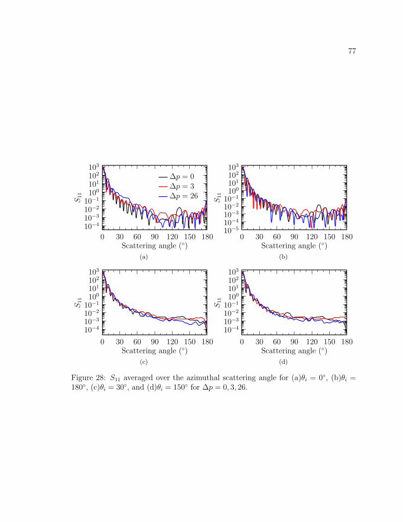
77

10−410−310−210−1100101102103

S11


∆p = 0∆p = 3∆p = 26

(a)

10−510−410−310−210−1100101102103

S11


(b)

10−410−310−210−1100101102103

S11


(c)

10−410−310−210−1100101102103

S11


(d)

Figure 28: S11 averaged over the azimuthal scattering angle for (a)θi = 0◦, (b)θi =180◦, (c)θi = 30◦, and (d)θi = 150◦ for ∆p = 0, 3, 26.

78

10−3

10−2

10−1

100

101

102

S11


(e)

10−3

10−2

10−1

100

101

102

S11


(f)

10−410−310−210−1100101102

S11


(g)

10−3

10−2

10−1

100

101

102

103

S11


(h)

Figure 28: S11 averaged over the azimuthal scattering angle for (e)θi = 60◦, (f)θi =120◦, (g)θi = 150◦, and (h)averaged over all θi for ∆p = 0, 3, 26.

79

−0.5

0

0.5

1

−S12/S

11


∆p = 0∆p = 3∆p = 26

(a)

0

0.5

1

−S12/S

11


(b)

0

0.5

−S12/S

11


(c)

0

0.5

1

−S12/S

11


(d)

Figure 29: −S12/S11 averaged over the azimuthal scattering angle for (a)θi = 0◦,(b)θi = 180◦, (c)θi = 30◦, and (d)θi = 150◦ for ∆p = 0, 3, 26.

80

0

0.5

−S12/S

11


(e)

0

0.5

1

−S12/S

11


(f)

0

0.5

−S12/S

11


(g)

0

0.5

−S12/S

11


(h)

Figure 29: −S12/S11 averaged over the azimuthal scattering angle for (e)θi = 60◦,(f)θi = 120◦, (g)θi = 150◦, and (h)averaged over all θi for ∆p = 0, 3, 26.

81

1

S22/S

11


∆p = 0∆p = 3∆p = 26

(a)

1

S22/S

11


(b)

0.98

0.99

1

S22/S

11


(c)

0.98

0.99

1

S22/S

11


(d)

Figure 30: S22/S11 averaged over the azimuthal scattering angle for (a)θi = 0◦, (b)θi =180◦, (c)θi = 30◦, and (d)θi = 150◦ for ∆p = 0, 3, 26.

82

0.96

0.97

0.98

0.99

1

S22/S

11


(e)

0.97

0.98

0.99

1

S22/S

11


(f)

0.95

0.96

0.97

0.98

0.99

1

S22/S

11


(g)

0.98

0.99

1

S22/S

11


(h)

Figure 30: S22/S11 averaged over the azimuthal scattering angle for (e)θi = 60◦,(f)θi = 120◦, (g)θi = 150◦, and (h)averaged over all θi for ∆p = 0, 3, 26.

83

−0.9−0.6−0.3

00.30.60.9

S33/S

11


∆p = 0∆p = 3∆p = 26

(a)

−0.9−0.6−0.3

00.30.60.9

S33/S

11


(b)

−1

−0.5

0

0.5

1

S33/S

11


(c)

−1

−0.5

0

0.5

1

S33/S

11


(d)


84

−1

−0.5

0

0.5

1

S33/S

11


(e)

−1

−0.5

0

0.5

1

S33/S

11


(f)

−1

−0.5

0

0.5

1

S33/S

11


(g)

−1

−0.5

0

0.5

1

S33/S

11


(h)


85

−0.5

0

0.5

1

S43/S

11


∆p = 0∆p = 3∆p = 26

(a)

−0.5

0

0.5

S43/S

11


(b)

−0.2

−0.1

0

0.1

0.2

S43/S

11


(c)

−0.2

−0.1

0

0.1

S43/S

11


(d)


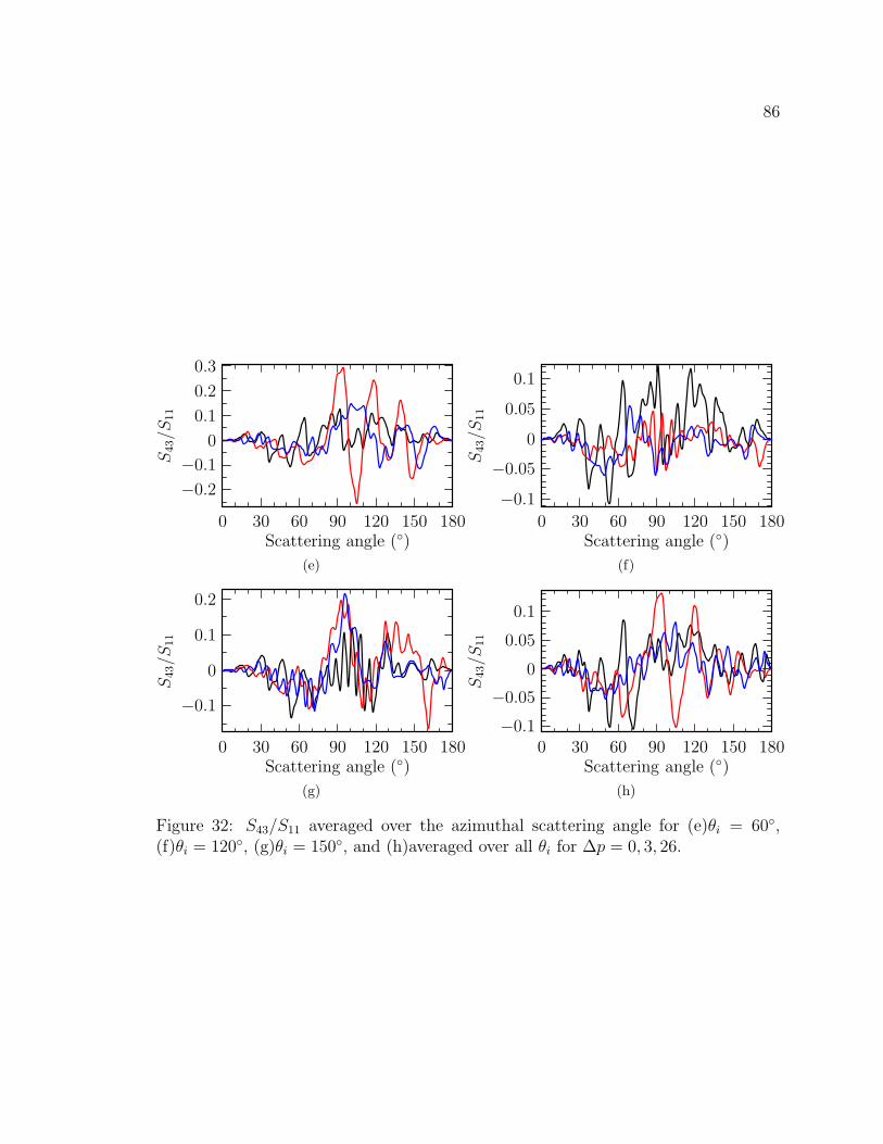
86

−0.2

−0.1

0

0.1

0.2

0.3

S43/S

11


(e)

−0.1

−0.05

0

0.05

0.1

S43/S

11


(f)

−0.1

0

0.1

0.2

S43/S

11


(g)

−0.1

−0.05

0

0.05

0.1

S43/S

11


(h)


87

the azimuthal angle with ∆p = 0, 3, 26 and for incident field angles of θ=0◦, 30◦,

90◦, 150◦, 180◦ and φi = 0 along with the result averaged over the incident angles.

For θi = 0◦, 180◦, the differing pressure gradients are clearly distinguishable, with

the exception of S22; however, for the other angles, there is no clear dependence

on the pressure gradient. For S22, the converse is true, i.e., the pressure gradients

are distinguishable for all angles except θ = 0◦, 180◦. These figures show that if

the orientation is known, there is sufficient information to differentiate the various

pressure gradients just as in the two-dimensional S11 figures. Unlike simulated models,

it is impractical to collect scattering data over the entire range of scattering angles in

laboratory testing. Also, determining the orientation of the RBC can be problematic

in the laboratory. Thus, the data of figures 28–32 which is averaged over the incident

field angles is the best candidate for practical use. This average behavior shows little

dependence on the pressure gradient, with the exception of S12 and S34.

Fig. 28 also gives evidence that the oscillations of S11 are related to the symmetry

of the particle. For θ = 0◦, 180◦, the RBC profile with respect to the incident field is

symmetric, and the characteristic oscillations are pronounced in the related figures.

For the other angles, where the profile is not symmetric, the oscillations are less

pronounced.

Chapter 9: NALM6 cells

9.1 Introduction

NALM6 cells are human B-cell precursors derived from the peripheral blood of a

patient with acute lymphoblastic leukemia[22]. B-cells are important biologically due

to their role in the immune system, part of which is to secrete antibodies in response

to invading microbes such as viruses or bacteria. B-cell comprise 10%–20% of the

lymphocyte population. Unactivated B-cells have a spherical shape with diameters

ranging from 6µm–9µm and a nuclei with diameters ranging from 5µm–8µm[42].

Activated B-cells, those en route to form plasma cells, are larger, having diameters

ranging from 9µm–15µm. These cells are larger due primarily to a greater amount of

cytoplasm.

For simulation, the NALM6 cells are modeled as two media, one corresponding

to the nucleus and the other to cytoplasm. These models are created from confocal

images using the process described in the next section to convert the confocal images

to domain images and then using the process described in §6 to create the model.

Once created, the models are assigned various refractive index values depending on

the purpose of the particular simulation.

9.2 Image acquisition and processing

To prepare the cells for imaging, they are stained with two dyes. The first dye,

FM 1-43 at 4µM , is absorbed by the cell membrane. The second dye, SYTO 61 at

5µM , is absorbed by the nucleus. FM 1-43 and SYTO 61 are excited at wavelengths

of 488nm and 633nm respectively. After staining, the cells are washed to remove

89

excess dye and placed in a depression slide. The imaging was done with a scanning

confocal microscope, the Zeiss LSM 510, using both a 488nm and a 633nm laser.

The fluorescence data was obtained on two independent channels corresponding to

the response of the two dyes. The images obtained are 512pixels×512pixels with each

pixel having an area of 0.04µm× 0.04µm. The separation between images is 0.51µm.

The images obtained for one of the cells, called cell #8, are shown in Fig. 33. In the

Figure 33: The set of confocal images for a cell #8. The green color indicates theresponse of the FM 1-43 dye and the red indicates the response of the SYTO 61 dye.

figure, the red indicates the response from SYTO 61, while the green indicates the

response of FM 1-43. The responses are scaled to an integer value between 0 and 255,

with a higher integer corresponding to a higher intensity. Analysis of the data revealed

that the green intensities were saturated in many of the pixels, i.e., the intensity was

90

higher than that associated with 255, and 255 is used. This makes the information

impractical for use in determining the domains; however, it was also determined that

the red data contained sufficient information to determine the nucleus and cytoplasm

domains. Fig. 34 shows only the red portion of the slide. In the image three distinct

intensity groups can be identified. The lowest intensity group corresponds to the

background, the medium intensity group to the cytoplasm, and the highest intensity

group to the nucleus. Thus, using the red data, the domains can be identified.

(a) (b)

Figure 34: (a)The original confocal image and (b)the same image showing only thered data. Using on the red data, three domains can be identified; the background,the cytoplasm, and the nucleus.

The process of converting the confocal images to domain images begins by identi-

fying the center of the cell. This is done by taking the first moment of intensity scaled

by the inverse of the total of all intensity values. Next, a histogram of the intensity

values for the slide closest to the center is taken. Fig. 35 shows the histogram for the

image of Fig. 34. Three peaks can be identified, corresponding to the background,

cytoplasm, and nucleus. Using the histogram, threshold values, intensity values which

91

separate the groups, are chosen. Next, two new sets of raster data are created with

the same size as that of the red data; these new sets will be referred to as the domain

sets. For the first domain set, all pixels belonging to the cytoplasm or nucleus groups,

according to the histogram, are given a value of one; and the remaining pixels are

given a zero value. For the second domain set, all pixels belonging to the nucleus

group are given a value of one; and the remaining pixels are given a zero value. Then

for each domain set, the single pixel specks are removed. This is done by comparing

the value of each pixel, to that of all of the pixel’s neighboring pixel values. If all

of the neighboring values are equal to each other and different from the pixel value,

then the pixel value is changed to that of its neighbors. The domain sets are then

“smoothed” using a window average with a two-dimensional Gaussian kernel. After

the smoothing, a threshold value is used to set all pixels to a value of zero or one. The

next step is to identify clusters in each of the domain sets. A cluster is a set of pixels

sharing the same value for which any pixel is “connected” to every other pixel by

pixels of the same value, i.e., if pixel 1 and neighboring pixel 2 have the same value;

and pixel 2 and its neighboring pixel 8 have the same value, then pixel 1 and pixel 8

are in the same cluster. Each cluster is given a unique value, and all pixels of a cluster

are assigned this value. The cluster containing the upper left corner of the image is

given a value of zero and is assumed to be part of the background. Finally, using the

domain sets with the cluster values, a new image is created with pixels which have a

green intensity value of 255, if the corresponding cytoplasm domain set pixel is not

part of the background cluster; and a red intensity value of 255, if the corresponding

nucleus domain set pixel is not part of the background cluster. All remaining pixels

are given green and red intensity values of 0. Fig. 36 shows the resultant image of this

process with the red image from Fig. 34 for comparison. The green area corresponds

to the cytoplasm and the yellow to the nucleus. The processed images can be used

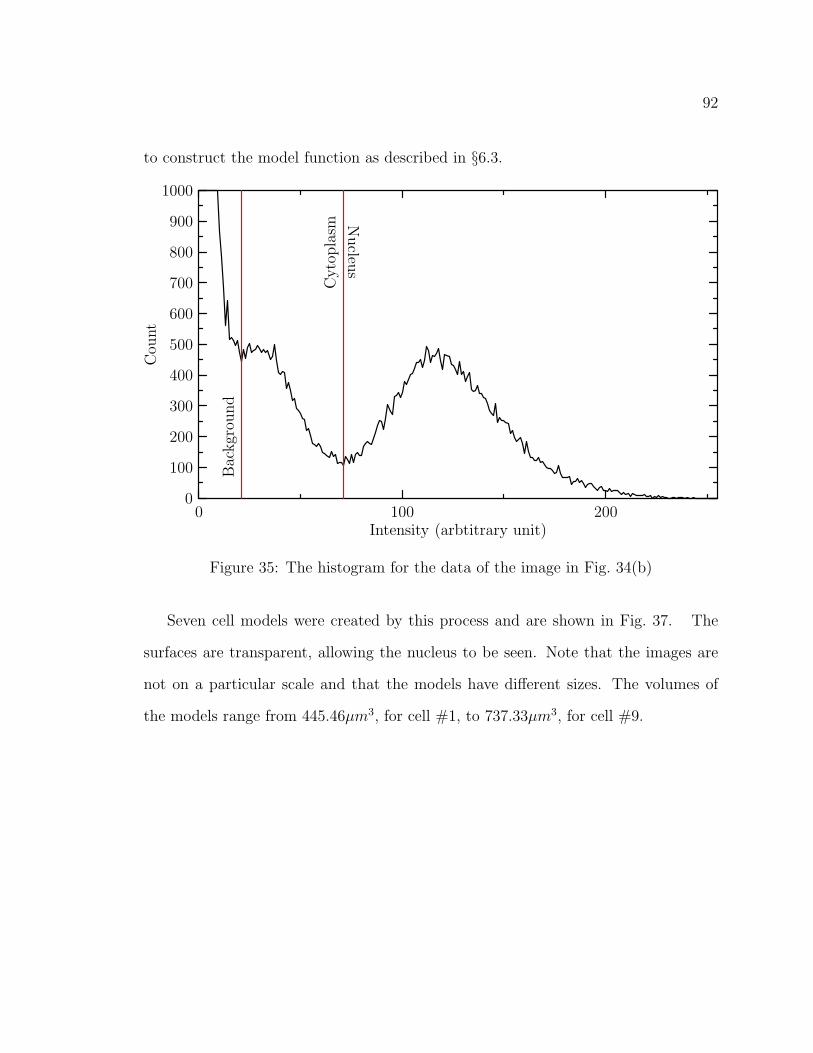
92

to construct the model function as described in §6.3.

0

100

200

300

400

500

600

700

800

900

1000

Cou

nt

0 100 200Intensity (arbtitrary unit)

Bac

kgr

ound

Cyto

pla

sm

Nucleu

s

Figure 35: The histogram for the data of the image in Fig. 34(b)

Seven cell models were created by this process and are shown in Fig. 37. The

surfaces are transparent, allowing the nucleus to be seen. Note that the images are

not on a particular scale and that the models have different sizes. The volumes of

the models range from 445.46µm3, for cell #1, to 737.33µm3, for cell #9.

93

(a) (b)

Figure 36: After processing the confocal image (b), a domain image (a) is produced.The domain image contains only the domain information; the intensity data is notincluded.

94

Figure 37: The confocal models for cell #s 1–10. The surfaces are transparent allowingthe model nucleus to be seen. The images are not on a particular scale; the smallestmodel, cell #1, has a volume of 445.46µm3, while the largest, cell #9, has a volumeof 737.33µm3.

95

9.3 Validation of models constructed from confo-

cal images

After constructing some cell models from confocal images, it was found that the

models were distorted due to optical distortions introduced in the image acquisition

process. This distortion results in stretching along the z-axis, causing the models

to appear elongated. In order to mitigate the deformation, model construction for

polystyrene spheres of known diameter were produced according to the procedures

described in §6.3 and §9.2. Commercially available spheres with a 6µm diameter that

are coated with a fluorescent dye were used for this purpose. Confocal images of a

sphere were acquired, shown in Fig. 38, under similar conditions to those in which

the NALM6 images were obtained. The images were processed and the sphere model

was constructed with the processed images. To partially offset the distortion intro-

duced in image acquisition, the distance between the images was scaled to produce a

nearly spherical shape. The sphere model as seen from three different viewpoints is

shown in Fig. 39. It can be seen from Fig. 39 that the sphere model is not perfectly

spherical. Two causes for this are the distortions introduced in the image acquisition

and errors introduced by the interpolation procedure. The scaling factor obtained via

this process is used to scale the images for biological cell as well.

To see how much the difference from a perfectly spherical shape affects the scatter-

ing pattern, the scattering phase function for the sphere model was calculated using

the FDTD method. The S11 matrix element for three angles of incidence along with

the average result is compared with that obtained from Mie theory for the scattering

from an ideal sphere of the same radius, 3µm, in Fig. 40. The simulations used an in-

cident wave of wavelength λ = 1µm in vacuum and a complex refractive index for the

sphere of n = 1.3675 + i1.0x10−5 in a host medium of refractive index of nh = 1.35.

96

Figure 38: The confocal images for a 6µm diameter sphere.

Figure 39: The confocal sphere model from three different viewpoints.

The FDTD grid cell size was set at ∆ = λh/30 with λh as the wavelength of the

incident light in the host medium. It can be seen from Fig. 40 that the results vary

depending on the angle of incidence. The sphere was oriented such that at incident

angle (θ = 0, φ = 0), the profile with respect to the incident wavefront is symmetric,

i.e., a circular shadow would be cast. Like the RBC data, this gives evidence to the

fact that the oscillations present in S11 are related to the symmetry of the particle.

These results demonstrate that the overall trend in the angular distribution of the

97

scattered light remains similar between the sphere model and a perfect sphere gener-

ated mathematically. The difference in the oscillation amplitudes can be attributed

to shape deformations inherent in the image acquisition and interpolation errors dur-

ing the model construction process. The characteristic oscillations in the scattering

phase function of a sphere are the direct consequence of the spherical symmetry of

the shape; thus, this feature is very sensitive to any departure from this symmetry.

A slight deformation introduced by the imperfect imaging and construction processes

is expected to cause observable changes in the details of the scattering pattern.

10−5

10−4

10−3

10−2

10−1

100

101

102

103

S11


Mieθ = 0◦, φ = 0◦

θ = 45◦, φ = 0◦

θ = 90◦, φ = 0◦

Average FDTD

Figure 40: A comparison of the scattering from a perfect sphere and the sphere modelobtained from confocal images.

In contrast, biological cells posses very little symmetry in their structures due

to their nonspherical shape, irregularities in the surface, and the heterogeneity of

the intracellular components. Thus, it is reasonable to expect that the imaging and

model construction errors observed in the case of the sphere should have much less

98

impact on the distributions of light scattered by cells. For example, the amplitude

of the cell membrane roughness, due to bending and folding, and other nonspherical

features in the shape of a typical B-cell observed by electron microscope[42] is typically

larger than the imaging and model construction errors of 0.3µm or less. Therefore,

it is much less likely in these cases than in the case of the sphere that such errors

will cause significant change in the light scattering patterns. It should be pointed

out that further improvement over the present work, which represents a first step in

constructing realistic 3D biological cell models for optical simulations, can be achieved

by refining the cell preparation, the image acquisition processes, and improving the

interpolation procedure.

99

9.4 Overview of the simulations

All of the cell model simulations discussed use the FDTD program prior to the dis-

persion correction, unless otherwise noted. To mitigate the effect of numerical errors

in comparing simulation results, all of the FDTD simulations discussed use identical

numerical parameters, i.e., those parameters not related to the physical system, such

as PML parameters. A PML layer of eight cells is used; preliminary studies showed

that this is sufficient. The number of cells between the smallest cuboid, aligned with

the grid axis, containing the cell model and the TF/SF boundary, see §3.2, is five.

The space between the TF/SF boundary and the inner PML boundary is eight cells

thick.

In addition, a common set of physical parameters is also used. The refractive

indices used for most of the simulations are 1.3500 for the host medium, 1.3675 +

i1.5×10−5 for the cytoplasm, and 1.4000+i1.5×10−5 for the nucleus. The purpose of

some of the simulations is to determine the effect of the refractive index on the result.

For these simulations the various refractive indices will be given in the discussion.

The angles of incidence used are also the same for all simulations. The set of

twelve incident angles used are

{(θi, φi)

∣∣ (θi, φi) ∈ {(28◦, 13◦) , (40◦, 236◦) , (45◦, 135◦) , (72◦, 306◦) ,

(77◦, 70◦) , (88◦, 187◦) , (93◦, 7◦) , (102◦, 250◦) ,

(107◦, 126◦) , (135◦, 315◦) , (139◦, 56◦) , (151◦, 193◦)}}

, (9.1)

where θi and φi are the polar and azimuthal angles with respect to the z-axis of the

FDTD grid, respectively. These angles were chosen to reduce proximity bias in the

results. Fig. 41 depicts the solid angle division among the incident angles. The equi-

lateral spherical pentagons represent the areas associated with the incident angles,

100

Figure 41: The incident angles used in the simulations are associated with equalportions of the solid angle. These portions are shown by the pentagonal tiling. Atthe center of each pentagon is a point where a ray at one of the incident anglesintersects the sphere.

while the points marked at the geometric center of the pentagons show where rays

at the incident angles intersect the sphere. Using this association, the results for

each incident angle represent an equal portion of the solid angle, and the distance

between any two neighboring angles is equal. Note that there are five such equilateral

polygonal tilings; specifically, tilings consisting of four, six, eight, twelve, and twenty

polygons. Preliminary testing showed negligible differences between the average re-

sults for the twenty angles and twelve angles and significant differences between those

of eight and twelve angles. Table 14 shows cext and g for these tests. Although g re-

mains almost the same, the percentage difference between the eight and twelve angle

cext results is 4.62%, while that between the twelve and twenty angle cext results is

0.424%. The incident field used in the simulations is a plane wave and approximates

101

Table 14: Average cext and average g for 8, 12, and 20 incident angles

no. of angles cext g8 4.1920 0.987312 4.0067 0.987420 3.9898 0.9873

a Gaussian pulse. The mean frequency of the pulse is the wavelength of interest.

The half-width of the pulse is equal in all simulations and is chosen to be as small as

possible to reduce the simulation time while maintaining numerical stability.

The grid discretization, ∆, and the CFL factor are λ/30 and 0.98 respectively.

Preliminary testing showed that ∆ = λ/30 allows for accurate results within a rea-

sonable simulation time. The ideal CFL factor is 1, and 0.98 was chosen to ensure

numerical stability while not significantly increasing the simulation time.

102

9.5 Volume dependence

To test the dependence of light scattering on the shape of the scattering particle,

scattering by the cell models is compared to scattering by sphere models. Two differ-

ent sphere models are used, the coated sphere and the equivalent sphere. The coated

sphere consists of concentric spheres, with the inner sphere having the same volume

and refractive index as the nucleus of the cell model. The outer sphere has the volume

of the entire cell model, and the region between the sphere surfaces is given the same

refractive index as the cytoplasm of the cell model. The equivalent sphere has the

same volume as the entire cell model and a refractive index that is the average of the

two refractive indices weighted by the respective volumes. The scattering result for

the cell models are obtained via the FDTD simulation. The sphere model results are

obtained from the program, DMILAY, by Toon and Ackerman which uses Mie theory

to calculate the result[43].

Fig. 42 shows S11, averaged over the azimuthal scattering angle, for the confocal

models and the sphere models, for all seven of the cells. For the confocal models, the

result shown is an average result for all of the incident angles listed in the previous

section. In each case, there is little difference between the various models for θ < 5◦.

This indicates that S11 at small scattering angles, < 5◦, is affected primarily by the

volume and refractive index and not by structural details[6]. This phenomenon has

also been reported in experimental studies of light scattering by biological cells[35].

For 5◦ < θ < 20◦, the coated sphere results and the confocal model results continue

to have little difference, while the equivalent sphere results show more oscillation.

This indicates that in this region, factors other than the volume and refractive index

contribute significantly to the scattering. The fact that the coated sphere and the

confocal model both contain a nucleus that the equivalent sphere lacks is evidence

103

that structural features affect the scattering in this region. Further, since the confocal

model and coated sphere nuclei differ in small-scale properties, such as surface fea-

tures, the scattering in this region is affected primarily by the large-scale properties,

such as volume. At angles greater than 20◦, both results from both types of sphere

models exhibit a larger amplitude of oscillation than that of the confocal models. This

is characteristic of the symmetries present in the sphere models. These differences

indicate that small-scale features also influence the scattering in this region[6]. The

differences between the results become progressively more pronounced with increasing

angle, which indicates that the influence of both large and small structural features

increases as the scattering angle increases.

Fig. 43 shows the confocal results for cell #8 at each of the incident angles along

with the results of the sphere models, which are the same at all angles. The cell #8

model’s “optical profile” is different when viewed from the various incident angles,

thus a different scattering pattern is expected. Although the scattering patterns are

different, the small difference in the results for θ < 20◦ at the various incident angles

lends further support to the conclusion that the scattering in this region is influenced

primarily by the volume and refractive index. Fig. 44 shows the confocal results for

cell #10 and the results of the associated sphere models. Although cell #8 and cell

#10 have nuclei with quite different shapes, see Fig. 37, the same conclusions can be

drawn from the cell #10 results. Comparison of each of the other five cell models

with their respective sphere model results are analogous to those of the cell #8 and

cell #10 models. Other comparisons to the sphere models can be made using the

S12, S33, and S43 elements. Fig. 9.5 shows the results for cell #8 and the associated

sphere models. The cell #8 result follows the same general trend as those of the

sphere models; however, it lacks the characteristic oscillations of the sphere models.

For the S12 and S33 elements this indicates that the large scale properties are the

104

primary influence for these elements. For the S43 element the magnitude of the cell

#8 result is almost flat, making it difficult to draw any conclusions.

Further support for the inflence of the volume on scattering can be seen by com-

paring the various cell models. Fig. 45 shows the average result for S11 (θ = 0.25◦)

plotted against volume for all of the cell models. Since the refractive index is the same

for each of the cell models, these results indicate that the scattering in the forward

direction is directly dependent on the volume.

By comparing S11 for the various cell models and their associated sphere models, it

is clear that the volume is a primary influence on scattering in the forward direction,

θ < 5◦. Also, comparisons between the cell models and the coated sphere show

that large scale properties, such as the presence of a nucleus, affect scattering over a

larger range, θ < 20◦. However, the equivalent sphere results suggest that the index

of refraction also influences scattering in the forward direction, since the equivalent

sphere has no nucleus and a different index of refraction.

105

10−410−310−210−1100101102103104105106

S11


Coated Sphere

Equivalent SphereAverage FDTD

(a)

100

101

102

103

104

105

106

S11

0 6.25 12.5 18.75 25Scattering angle (◦)

(b)

10−510−410−310−210−1100101102103104105106

S11


(c)

100

101

102

103

104

105

106

S11


(d)

10−510−410−310−210−1100101102103104105106

S11


(e)

100

101

102

103

104

105

106

S11


(f)

Figure 42: S11 of the cell models and the sphere models for (a,b)cell #1, (c,d)cell #2,(e,f)cell #3.

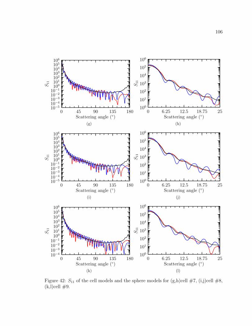
106

10−510−410−310−210−1100101102103104105106

S11


(g)

100

101

102

103

104

105

106

S11


(h)

10−510−410−310−210−1100101102103104105106

S11


(i)

100

101

102

103

104

105

106

S11


(j)

10−410−310−210−1100101102103104105106

S11


(k)

100

101

102

103

104

105

106

S11


(l)

Figure 42: S11 of the cell models and the sphere models for (g,h)cell #7, (i,j)cell #8,(k,l)cell #9.

107

10−510−410−310−210−1100101102103104105106

S11


(m)

100

101

102

103

104

105

106S

11


(n)

Figure 42: S11 of the cell models and the sphere models for (m,n)cell #10.

108

10−5

10−4

10−3

10−2

10−1

100

101

102

103

104

105

106S

11


Coated Sphere Equivalent Sphereθ = 28◦, φ = 13◦ θ = 40◦, φ = 236◦

θ = 45◦, φ = 135◦ θ = 72◦, φ = 306◦

θ = 77◦, φ = 70◦ θ = 88◦, φ = 187◦

θ = 91◦, φ = 7◦ θ = 102◦, φ = 250◦

θ = 107◦, φ = 126◦ θ = 135◦, φ = 315◦

θ = 139◦, φ = 56◦ θ = 151◦, φ = 193◦

Average FDTD

100

101

102

103

104

105

106

S11


Figure 43: The S11 result for the simulations with confocal model and sphere modelsof cell #8. There is little difference in the results for θ < 5◦, while the coated spheremodel and the confocal model continue to show little difference up to θ ≈ 20◦.

109

10−5

10−4

10−3

10−2

10−1

100

101

102

103

104

105

106S

11


Coated Sphere Equivalent Sphereθ = 28◦, φ = 13◦ θ = 40◦, φ = 236◦

θ = 45◦, φ = 135◦ θ = 72◦, φ = 306◦

θ = 77◦, φ = 70◦ θ = 88◦, φ = 187◦

θ = 91◦, φ = 7◦ θ = 102◦, φ = 250◦

θ = 107◦, φ = 126◦ θ = 135◦, φ = 315◦

θ = 139◦, φ = 56◦ θ = 151◦, φ = 193◦

Average FDTD

100

101

102

103

104

105

106

S11


Figure 44: The S11 result for the simulations with confocal model and sphere modelsof cell #10. There is little difference in the results for θ < 5◦, while the coated spheremodel and the confocal model continue to show little difference up to θ ≈ 20◦.

110

−1

−0.5

0

0.5

1−S

12/S

11


Coated SphereEquivalent SphereAverage FDTD

(a)

−1

−0.5

0

0.5

1

S33/S

11


(b)

111

−1

−0.5

0

0.5

1

S43/S

11


(c)

Figure 44: S12, S33, and S43 for the confocal model and sphere models of cell #8. Theresults in each case have the same general trend; however the confocal model doesnot show the characteristic oscillations due to symmetry.

112

400

500

600

700

800

S11(θ

=0.

25◦ )

1×105 1.5×105 2×105 2.5×105 3×105

Volume (∆3)

Figure 45: S11(θ = 0.25◦) vs. volume for each of the confocal models. This indicatesthat the forward scattering is influenced primarily by the volume for a given refractiveindex.

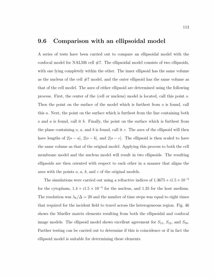
113

9.6 Comparison with an ellipsoidal model

A series of tests have been carried out to compare an ellipsoidal model with the

confocal model for NALM6 cell #7. The ellipsoidal model consists of two ellipsoids,

with one lying completely within the other. The inner ellipsoid has the same volume

as the nucleus of the cell #7 model, and the outer ellipsoid has the same volume as

that of the cell model. The axes of either ellipsoid are determined using the following

process. First, the center of the (cell or nucleus) model is located, call this point o.

Then the point on the surface of the model which is furthest from o is found, call

this a. Next, the point on the surface which is furthest from the line containing both

o and a is found, call it b. Finally, the point on the surface which is furthest from

the plane containing o, a, and b is found, call it c. The axes of the ellipsoid will then

have lengths of 2|o − a|, 2|o − b|, and 2|o − c|. The ellipsoid is then scaled to have

the same volume as that of the original model. Applying this process to both the cell

membrane model and the nucleus model will result in two ellipsoids. The resulting

ellipsoids are then oriented with respect to each other in a manner that aligns the

axes with the points o, a, b, and c of the original models.

The simulations were carried out using a refractive indices of 1.3675 + i1.5× 10−5

for the cytoplasm, 1.4 + i1.5 × 10−5 for the nucleus, and 1.35 for the host medium.

The resolution was λh/∆ = 20 and the number of time steps was equal to eight times

that required for the incident field to travel across the heterogeneous region. Fig. 46

shows the Mueller matrix elements resulting from both the ellipsoidal and confocal

image models. The ellipsoid model shows excellent agreement for S11, S12, and S33.

Further testing can be carried out to determine if this is coincidence or if in fact the

ellipsoid model is suitable for determining these elements.

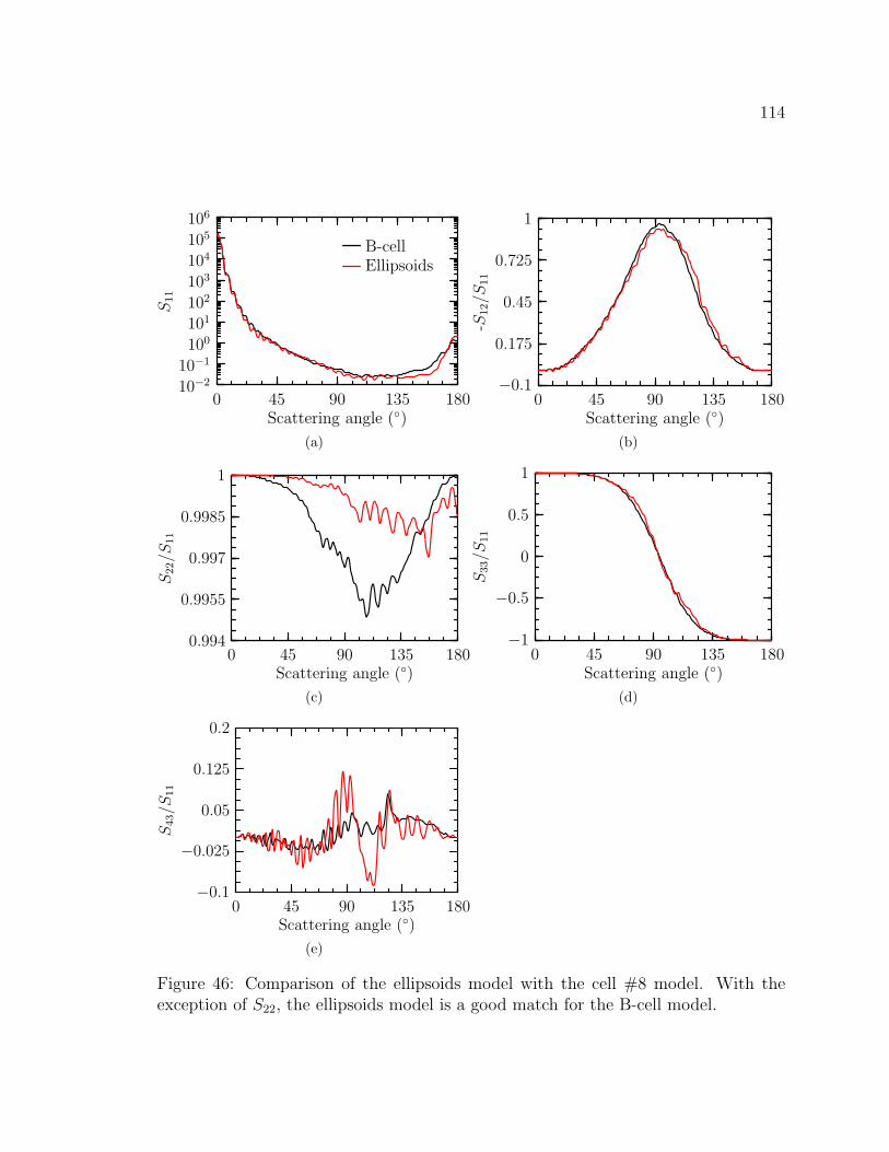
114

10−2

10−1

100

101

102

103

104

105

106

S11


B-cellEllipsoids

(a)

−0.1

0.175

0.45

0.725

1

-S12/S

11


(b)

0.994

0.9955

0.997

0.9985

1

S22/S

11


(c)

−1

−0.5

0

0.5

1S

33/S

11


(d)

−0.1

−0.025

0.05

0.125

0.2

S43/S

11


(e)

Figure 46: Comparison of the ellipsoids model with the cell #8 model. With theexception of S22, the ellipsoids model is a good match for the B-cell model.

115

9.7 Dependence on the nucleus and refractive in-

dex

In the previous section, it was found that light scattering in the forward direction is

influenced primarily by the volume and refractive index of the scattering particle. To

isolate the effect of the refractive index, simulations with cell models using three

different refractive indices for the nucleus have been carried out. The refractive

indices are 1.3675, 1.4000, and 1.4325. Note that using 1.3675 as the refractive index

effectively eliminates the nucleus since it is not optically distinct from the cytoplasm.

In addition, results for the nucleus alone at refractive indices of 1.4000 and 1.4325

have also been obtained.

10−3

10−2

10−1

100

101

102

103

104

105

106

S11


Cell nn = 1.3675Cell nn = 1.4000Cell nn = 1.4325Nucleus nn = 1.4000Nucleus nn = 1.4325

Figure 47: S11 result for the confocal model of cell #8 with various refractive indicesfor the nucleus. As the refractive index increases, the nucleus becomes the dominantfactor in scattering intensity.

116

Fig. 47 shows the S11 results for the cell #8 model. It can be seen that the cell

model with no nucleus scatters less than either model with a nucleus over the entire

range. At θ < 5◦, the results for the models having a nucleus show little difference,

indicating that the presence of a nucleus contributes significantly to the scattering in

this region. Further, the difference between the results for the model with a nucleus

and the model of the nucleus alone is less for the higher refractive index than for

the lower. This indicates that as the refractive index increases, the nucleus becomes

the primary influence on the scattering. The effect of the nucleus can also be seen

in the scattering cross section results, shown in Fig. 48. For the model with a lower

0

50

100

150

200

Cell onlyNucleus only

Cell and nucleus

nnucl = 1.4000ncyto = 1.3675

nnucl = 1.4325ncyto = 1.3675

Figure 48: csca results for the confocal model of cell #8. Taking the sum of the crosssections for the cell and nucleus, shows that for the lower index, the cell and nucleustogether act to scatter more light than the sum of the individual results. For thehigher index, the nucleus is primarily responsible for the scattering.

index, the sum of the scattering cross sections for the nucleus and cell is a little more

117

than half of the result for the cell with a nucleus, indicating that the presence of the

nucleus within the cell model causes more scattering than can be accounted for by

the nucleus alone. For the higher index, the nucleus dominates the scattering as the

index increases, since the scattering by the nucleus alone is only a little less than the

scattering by the cell with the nucleus. This can also be seen in the S11 result by

looking at the difference between the cell models and the associated nucleus models.

For the higher index, the difference for the higher index models is less than that of

the lower index models over almost the entire range.

−0.1

0.175

0.45

0.725

1

−S12/S

11



Figure 49: S12 result for the confocal model of cell #8 with various refractive indices.As the refractive index of the nucleus increases, the peak magnitude decreases andthe peak shift to a wider angle.

Fig. 49 shows the S12 results for the cell #8 model, where another effect of the

index of the nucleus can be seen. Like the S11 results, the S12 results show that the

118

result for the models with the higher index show less difference than those of the

lower index. In addition, the S12 result shows that as the index increases, the peak

in the results shifts becoming lower and occurring at a wider angle. This information

in conjunction with the information obtained from the S11 result could be used to

determine the volume and refractive index of the cell.

The cell #1, cell #7, cell #9, and cell #10 models were all tested in the same

manner as the cell #8 model. Analysis of these models is analogous to that of the

cell #8 model and results in the same conclusions. Fig. 50 shows the S11, S12, and

scattering cross section results for the cell #10 model for reference.

The effect of the nucleus and index of refraction can also be seen by analyz-

ing the S11 result at particular scattering angles. Fig. 51 shows S11 (θ = 0.25◦) vs.

(a)∫ 45◦

25◦ S11dθ, (b)∫ 110◦

90◦ S11dθ, and (c)∫ 178◦

158◦ S11dθ for all of the cell models with a nu-

cleus having refractive index of 1.4000 and with the additional models having various

refractive indices for cell #9 and cell #10. Each point in the plot represents the

result at one of the twelve incident angles discussed previously. As expected, from

the previous discussion, the models having the same index are separated vertically

according to their respective volumes; also, some horizontal separation indicates that

the scattering at 25◦ < θ < 45◦ and 90◦ < θ < 110◦ indicates a volume dependence as

well. However, the models having a higher index of refraction have points separated

by only a small amount vertically, but by a larger separation horizontally. Also, the

horizontal separation is more pronounced with an increasing index. Together, these

indicate the previous conclusion that volume is a primary factor in the forward scat-

tering direction, but in addition, these data indicate that scattering at 25◦ < θ < 110◦

is affected to a greater extent by the refractive index, rather than the volume. The

data of these plots is typical of the type of data gathered by the use of flow cytometry.

This gives another avenue into the determination of volume and index of refraction

119

via the combination computational and experimental research.

Another phenomenon seen in Fig. 51 is the spread of the points for a particular

cell. From the three-dimensional visualizations of Fig. 37, it can be seen that the

nuclei of cell #9 and cell #10 have a more complex structure than those of the other

cells. Again referring to Fig. 51, this manifests as a wider spread in the distribution of

the points associated with these models when compared to those with a more spherical

nuclear structure. This indicates that for cells with a complex nuclear structure, the

difference in scattering results for the various angles is larger than those with the less

complicated structure.

120

10−3

10−2

10−1

100

101

102

103

104

105

106

S11



−0.1

0.175

0.45

0.725

1

−S12/S

11


0

75

150

225

300

Cell onlyNucleus only

Cell and nucleus

nnucl = 1.4000ncyto = 1.3675

nnucl = 1.4325ncyto = 1.3675

Figure 50: The results obtained using the confocal model of cell #10, lead to thesame conclusions as those determined for cell #8, although cell #8 and cell #10 havenuclei which differ in shape.

121

1×105

1.75×105

2.5×105

3.25×105

4×105S

11(θ

=0.

25◦ )

0 225 450 675 900∫ 45◦

25◦ S11dθ

Cells 9,10nnucl = 1.4325


Cells 1,2,3,7,8nnucl = 1.4000

(a)

1×105

1.75×105

2.5×105

3.25×105

4×105

S11(θ

=0.

25◦ )

0 1.75 3.5 5.25 7∫ 110◦

90◦ S11dθ



Cells 1,2,3,7,8nnucl = 1.4000

(b)

Figure 51

122

1×105

1.75×105

2.5×105

3.25×105

4×105

S11(θ

=0.

25◦ )

−10 15 40 65 90∫ 178◦

158◦ S11dθ

(c)

Figure 51: The scatter plot of S11(θ = 0.25◦) vs. (a)∫ 45◦

25◦ S11dθ, (b)∫ 110◦

90◦ S11dθ, and

(c)∫ 178◦

158◦ S11dθ. From (a) and (a) the cells having a complex nucleus or a higherrefractive index can be identified.

123

9.8 Internal nuclear structure dependence

From the results presented in the previous section, it is apparent that internal struc-

ture, specifically the nucleus, has a direct effect on the scattering by cells. The next

step in this investigation is to determine if structures within the nucleus will affect

the scattering similarly. To test this, cell models with an inhomogeneous nucleus have

been simulated. Recall from §9.2 that the intensity of the red component of the pixel

data corresponds to the response of the SYTO 61 dye which is found in higher con-

centrations within the nucleus. Assuming that this concentration is associated with

the refractive index allows structures within the nucleus to be modeled. Although

further investigation is needed to determine the validity of such an assumption, this

investigation can still show trends in scattering results due to the presence of internal

structure.

To test the dependence on internal structure, four types of nucleus models are used.

These will be referred to as the unfiltered model, the 0.71 model, the 0.90 model, and

the 2-bin model. The unfiltered, 0.71, and 0.90 models are given internal structure

by transforming the confocal images and removing the high frequency components

(possibly none), which will be discussed. The 2-bin model also gives internal structure

to the nucleus, but does so by dividing the pixels within the nucleus domain into two

groups and assigning a different index of refraction to each one, also to be discussed.

Construction of the unfiltered, 0.71, and 0.90 models begins in the same manner

as previously discussed, see §6, by analyzing the images and determining which pixels

belong to the cytoplasm domain and which pixels belong to the nucleus domain.

Next, the confocal images are transformed using a Fourier transform to give the

spatial frequency components of the images. Then, a filter is applied to remove

the high frequency components. This process is depicted in Fig. 52. Fig. 52b

124

(a) (b)

(c)

Figure 52: To simulate nuclear structure, the original image(a) is filtered by cuttingout high-frequency componets. (c)The image obtained by applying the filter depictedin (b).

125

shows the transformed image with the filter applied. The difference between the

unfiltered, 0.71, and 0.90 models is in the number of high frequency components

removed. 0.71 and 0.90 refer to the length of the line segment “r” shown in the figure,

and the unfiltered model has r = 1. Thus, the unfiltered image has no components

removed, while the 0.90 model has fewer frequency components removed than the 0.71

model. Following the removal of the high frequency components, the altered image is

transformed using an inverse Fourier transform to give a new spatial domain image,

as seen in Fig. 52c. Comparison of the initial and final images shows that the final

image has less variation in the intensity distribution, resulting in a more “clustered”

structure within the nucleus. After the transformation, the various intensity values

are associated with a refractive index. To do this, a function is derived which maps the

intensity value to the refractive index according to constraints which limit the average

and maximum difference of the refractive index values. More specifically, given an

average refractive index of n, a maximum difference of ∆ (Im − I1), Ni points having

intensity Ii, i = 1, 2, · · · ,m, and a characteristic function f , find ni such that

∑i

Nini = n∑i

Ni

ni = n1 + ∆f (Ii)− f (I1)

f (Im)− f (I1),

(9.2)

which has the solution

ni = n+∆

f (Im)− f (I1)

(f (Ii)−

∑j Njf (Ij)∑

j Nj

). (9.3)

The average refractive index used is 1.4000, and ∆ is chosen as 0.04. Two character-

istic functions have been used; the identity function, Id, and the natural logarithm,

ln. Fig. 53 shows an example of the mapping using these characteristic functions.

126

1.37

1.385

1.4

1.415

1.43

nnucl

0 50 100 150 200Intensity

lnid

Figure 53: Two characteristic functions are used to determine the refractive indexassociated with the various intensities within the nucleus.

The construction process continues as previously described with the exception that

voxels located between slides have an interpolated index of refraction rather than a

strict inside/outside criterion.

Construction of the 2-bin model also begins in the same manner as previously

described. Once the domains have been identified, the pixels of the nucleus domain

are divided into two groups according to whether their associated intensities are

higher or lower than some cut-off value. The pixels of higher intensity are given an

index of refraction of 1.4325 and those of lower intensity are given an index of 1.3675.

The cut-off value is determined such that the average refractive index is 1.4000. The

construction process then continues with voxels located between slides assigned a

value determined by whether the interpolated intensity is lower or higher than the

cut-off value.

Fig. 54 shows model cross sections for the unfiltered, 0.71, and 2-bin models in

the xy, xz, and yz planes passing through the center of the model. Since the original

images are in the xy-plane, the best resolution is seen in this plane. The xz and yz

planes show the blending of the data for voxels located between the images.

Simulations have been carried out using the cell #8 model with an inhomogeneous

127

Figure 54: Domain images showing the nuclear structure resulting from (top row)nofiltering, (middle row)r = 0.71(ln) filtering, and (bottom row) a 2-bin model. Threedifferent cross-sections are shown, (left column)xy-plane, (middle column)xz-plane,and (right column)yz-plane.

128

nucleus. The nucleus models used are the unfiltered, 0.71 Id, 0.71 ln, and 0.90 ln

models. A 2-bin model has been constructed, but results have not yet been obtained

for this model. Fig. 55 shows a comparison of S11 and S12 for the homogeneous,

10−210−1100101102103104105106

S11

0 20 40 60 80 100120140160180Scattering angle (◦)

homogeneous

id r = 0.71ln r = 0.71

−0.5

0

0.5

1

S12/S

11


Figure 55: The natural log and identity models

Figure 56: Little difference can be seen in S11(left) and S12(right) for natural log andidentity models.

0.71 Id, and 0.71 ln models. The results are almost identical and there is no obvious

way to discriminate between any of the models. This could be due to the choice of ∆ =

0.04 resulting in a “smooth” spatial distribution in the index of refraction. Fig. 57

10−210−1100101102103104105106

S11


homogeneous

ln r = 0.71ln r = 0.90

ln r = 1.00

−0.5

0

0.5

1

S12/S

11


Figure 57: Little difference can be seen in S11(left) and S12(right) for natural logmodels created with differing filters.

shows the comparison for all of the ln model results along with the homogeneous

result. Like Fig. 55, there is little difference in the scattering by the various models.

129

The other Mueller matrix elements also show little difference between the various

models.

Recall from the previous section that a plot of S11 (θ = 0.25◦) vs. S11 (θ = 35◦)

allowed discrimination between nuclei having various refractive indices. Fig. 58 shows

1×105

1.75×105

2.5×105

3.25×105

4×105

S11(θ

=0.

25◦ )

0 50 100 150 200∫ 45◦

25◦ S11dθ

id r = 0.70ln r = 0.70ln r = 0.90ln r = 1.00

Figure 58: Forward vs. 25◦−45◦ scattering shows that the models having an inhomo-geneous nucleus are not distinguishable from those having a homogeneous nucleus.

S11 (θ = 0.25) vs.∫ 45◦

25◦ S11 (θ) dθ for the homogeneous and inhomogeneous models of

cell #8. Using this analysis is also not helpful in distinguishing the various models.

Recall from Eq. (2.6) that a change in ε results in a different scattered field.

Although the scattered field must be different for the various models, this difference

is not obvious in the Mueller matrix elements. Further investigation using a larger

value for ∆ or using an additional stochastic process to determine the refractive index

between slides may help in understanding the circumstances under which observable

130

changes in the Mueller matrix will occur.

131

9.9 Comparison with experimental results

Experiments to determine the Mueller matrix for NALM6 cells have been carried out

at the Biomedical Laser Laboratory at East Carolina University[13]. The cells used

in the experiment are from the same cell line, NALM6, and from the same source as

those used for the computational results. A dilute solution of about 2.34×102cells/µL

was used to obtain results that approximate those of single scattering events. For

experimental details refer to [13].

10−3

10−2

10−1

100

S11


633nm850nm

−0.5

0

0.5

1

−S12/S

11


10−210−1100101102103104105106

S11


633nm850nm

−0.5

0

0.5

1

−S12/S

11


Figure 59: The experimental results(top) and simulation results(bottom) differ inbehavior. For S11 the 850nm and 633nm curves show differences in the sidescatteringregion. For S12, both show a peak shift to the right for the lower wavelength; however,the magnitude peaks are not in agreement.

Fig. 59 shows the experimental results for wavelengths of 850nm and 633nm

along with the FDTD results for the cell #8 model. For the FDTD simulations at

850nm, 1.330[13] was used as the refractive index of the host medium, 1.368 for the

cytoplasm[9], and 1.400[8] for the nucleus. For the simulations at 630nm, 1.336 was

132

used as the refractive index of the host medium, 1.380 for the cytoplasm, and 1.430

for the nucleus. The S11 results differ in the side scattering region, 60◦ < θ < 120◦,

where the experimental results show that the 850nm scattering is greater than that

of 633nm. The S12 results are also quite different. The experimental result shows

the peak for the 850nm result is lower and to the left of that of the 633nm result;

while the FDTD result shows the 850nm peak being higher and to the right of that

of the 633nm. One possible reason for the differences is that the computational

results are for a single cell, whereas the experimental results are for a large group of

cells. Although the experimental results approximate single scattering, the result is

an average result of many approximate single scattering events. Another possibility

is that some physical cell structure that is not modeled in the simulation, such as

the cell membrane, affects the scattering to an extent that significantly changes the

results.

Further investigation is needed to resolve the differences between the experimental

results and computational results. Such investigation could include adding a cell

membrane and/or an endoplasmic reticulum to the cell model. Previous studies show

that the cell membrane has a refractive index of 1.46[28], significantly higher than

that of the cytoplasm, 1.36. Future investigation could also vary the refractive index

of each component of the cell model to determine the influence on the scattering.

Chapter 10: Conclusion

Understanding light scattering from biological cells is critical to furthering research

that will help in the diagnosis and treatment of diseases such as cancer. Because

most biological cells have size parameters approximately the same as the wavelength

of the light used to analyze them, the wave nature of the light must be taken into

account when modeling the light-cell interaction. A program has been developed to

simulate the interaction and return results in the form of cross sections, anisotropy

factor, and Mueller matrix. The program implements the FDTD method, which was

chosen for suitability in simulating scattering from particles with sizes over a range

which includes most biological cells. Parallel methods have been employed, allowing

more computational resources to be used in simulating the interaction.

The basis of the FDTD method is the replacement of continuous derivative oper-

ators with finite difference operators. This allows systems having complicated shapes

to be simulated without having to obtain simultaneous solutions and without hav-

ing to use complicated boundary conditions at the “edges” of the scattering particle.

The method has been in use in many areas of research for decades and thus has large

body of supporting literature and development. The implementation of the FDTD

method uses a cubic grid which allows parallel methods to be easily implemented

along planes of the grid. The program has been validated against Mie theory calcu-

lations. Berrenger’s perfectly matching layer absorbing boundary condition is used

to terminate the grid. The simulation time and parallel efficiency have also been

evaluated, and it was shown that the program can produce realistic scattering results

within a reasonable time frame.

Models of red blood cells having various shapes, due to pressure, have been created.

Simulations using the models have shown that the shape of the scattering particle is

134

a primary factor in the scattering of light. However, it was found that for practical

purposes, further study is needed to be able to distinguish these shapes according to

their “average” behavior. These simulations also gave evidence that the peaks and

valleys of the S11 matrix element are related to the symmetry of the particle.

Two other programs have been created to model cells using confocal images. One

of these uses the data obtained from the confocal microscope to produce a set of do-

main images. The other takes the domain images and produces a three-dimensional

model. These models are then input into the FDTD program along with the refrac-

tive index values. Seven different B-cell models have been created. The results of

the simulations carried out using these models have shown that both homogeneous

and coated sphere models are not suitable substitutes for actual B-cell models when

determining the Mueller matrix elements at scattering angles greater than 20◦. An

ellipsoid model has also been tested, and it was found that the ellipsoid model is suit-

able for the calculation of matrix elements S11, S12, and S33. Using all of the models,

it was shown that scattering at small angles is influenced primarily by the global

properties of the shape of the scattering particle such as the volume and the presence

of the nucleus. The dependence on small scale properties such as variations in the

refractive index of the nucleus was also tested. A comparison of the results showed

little difference for various nuclei simulated; however, the variation in the refractive

index was small and further testing may reveal differences when using larger varia-

tions. Finally, a comparison with experimental results revealed discrepancies. Further

computational testing using average Mie theory results showed the same behavior as

that of the FDTD results. Further experimental data and more comprehensive B-cell

simulation (using more than seven models) are needed to resolve these discrepancies.

Bibliography

[1] V. Backman, R. Gurjar, K. Badizadegan, I. Itzkan, R. Dasari, l. Perelman, and

M. Feld. Polarized light scattering spectroscopy for quantitative measurement of

epithelial cellular structures in situ. IEEE Journal of Selected Topics in Quantum

Electronics, 5:1019–1026, 1999.

[2] C. Bohren and D. Huffman. Absorption and scattering of light by small particles.

John Wiley & Sons, New York, 1983.

[3] A. G. Borovoi, E. I. Naats, and U. G. Oppel. Scattering of light by a red blood

cell. Journal of Biomedical Optics, 3:364–372, 1998.

[4] C. D. Bortner and J. A. Cidlowski. Methods in Cell Biology, chapter Flow cyto-

metric analysis of cell shrinkage and monovalent ions during apoptosis. Academic

Press, San Diego, 2000.

[5] R. S. Brock, X.-H. Hu, P. Yang, and J. Q. Lu. Evaluation of a parallel FDTD

code and application to modeling of light scattering by deformed red blood cells.

Optics Express, 13:5279–5292, 2005.

[6] R. S. Brock, X.-H. Hu, D. A. Weidner, J. R. Mourant, and J. Q. Lu. Effect of

detailed cell structure on light scattering distribution: FDTD study of a B-cell

with 3D structure reconstructed from confocal images. Journal of Quantitative

Spectroscopy & Radiative Transfer, 102:25–36, 2006.

[7] J. P. Brooks, K. K. Ghosh, E. Harrigan, D. S. Katz, and A. Taflove. Com-

putational electromagnetics and supercomputer architecture, PIERS, chapter

Progress in Cray-based algorithms for computational electromagnetics, pages

23–55. EMW Publishing, 1993.

136

[8] A. Brunsting and P. Mullaney. Differential light scattering from spherical mam-

malian cells. Biophysical Journal, 14:439–453, 1974.

[9] J. Bruthan, O. Minet, J. Helfmann, M. Herrig, and G. Muller. The spatial

variation of the refractive index in biological cells. Physics in Medicine and

Biology, 41:369–382, 1996.

[10] C. Chen, J. Q. Lu, H. Ding, K. M. Jacobs, Y. Du, and X.-H. Hu. A primary

method for determination of optical parameters of turbid samples and application

to intralipid between 550 and 1630 nm. Optics Express, 14:7420–7435, 2006.

[11] K. C. Chew and V. F. Fusco. A parallel implementation of the finite-difference

time-domain algorithm. International Journal of Numerical Modeling: Electronic

Networks, Devices and Fields, 8:293–299, 1995.

[12] K. S. de Boer, M. A. Jura, and M. J. Shull. Exploring the universe with the

IUE satellite, chapter Diffuse and dark clouds in the interstellar medium, pages

485–515. D. Reidel Publishing Co., Dordrecht, 1987.

[13] H. Ding, J. Q. Lu, R. S. Brock, T. J. McConnell, J. F. Ojeda, K. M. Jacobs, and

X.-H. Hu. Angle-resolved Mueller matrix study of light scattering by B-cells at

three wavelengths of 442, 633 and 850nm. Journal of Biomedical Optics, to be

published.

[14] R. Drezek, A. Dunn, and R. Richards-Kortum. Light scattering from cells: finite-

difference time-domain simulations and goniometric measurements. Applied Op-

tics, 38:3651–3661, 1999.

[15] P. S. Excell, A. D. Tinniswood, and K. Haigh-Hutchinson. Parallel computa-

137

tion of large-scale electromagnetic field distributions. Applied Computational

Electromagnetics Society Journal, 13:179–187, 1998.

[16] S. D. Gedney. Finite-difference time-domain analysis of microwave circuit de-

viceson high performance vector/parallel computers. IEEE Transactions on Mi-

crowave Theory and Techniques, 43:2510–2514, 1995.

[17] G. H. Goedecke and S. G. OBrien. Scattering by irregular inhomogeneous parti-

cles via the digitized Greens function algorithm. Applied Optics, 15:2431–2437,

1988.

[18] R. Guerrieri, R. K. Tadros, J. Gamelin, and A. Neureuther. Massively parallel

algorithms for scattering in aptical lithography. IEEE Trans. Computer-Aided

Design, 10:1091–1100, 1991.

[19] A. Hoekstra, B. Hertzberger, and P. Sloot. The optical “fingerprints” of cells:

Catching the bad guys. IEEE Computational Science & Engineering, 3:4–5, 1996.

[20] A. G. Hoekstra, V. P. Maltsev, and G. Videen, editors. Optics of Biological

Particles. Springer, London, 2007.

[21] H. Hoteit, R. Sauleau, B. Philippe, P. Coquet, and J. P. Daniel. Vector and par-

allel implementations for the FDTD analysis of millimeter wave planar antennas.

International Journal of High Speed Computing, 10(2):209–234, 1999.

[22] H. R. Hurwitz, J. Hozier, T. LeBien, J. Minowada, K. Gajl-Peczalska, I. Kubon-

ishi, and J. Kersey. Characterization of a leukemic cell line of the pre-B pheno-

type. International Journal of Cancer, 23:174–180, 1979.

[23] J. D. Jackson. Classical Electrodynamics. John Wiley & Sons, New York, 3

edition, 1998.

138

[24] J. Q. Lu, P. Yang, and X.-H. Hu. Simulations of light scattering from a biconcave

red blood cell using the FDTD method. Journal of Biomedical Optics, 10:2431–

2437, 2005.

[25] J. Q. Lu, R. S. Brock, P. Yang, and X.-H. Hu. Optics of Biological Particles,

chapter Modeling of light scattering by single red blood cells with an FDTD

method. Springer, London, 2007.

[26] J. Lumpp, S. K. Maxumdar, and S. D. Gedney. Performance modeling of the

finite-difference time-domain method on parallel systems. ACES Journal.

[27] X. Ma, J. Q. Lu, R. S. Brock, K. M. Jacobs, P. Yang, and X.-H. Hu. Determi-

nation of complex refractive index of polystyrene microspheres from 370 to 1610

nm. Physics in Medicine and Biolog, 48:4165–4172, 2003.

[28] J. Maier, S. Walker, S. Fantini, M. Franceschini, , and E. Gratton. Possible corre-

lation between blood glucose concentration and the reduced scattering coefficient

of tissues in the near infrared. Optics Letters, 19:2062–2064, 1994.

[29] V. P. Maltsev. Scanning flow cytometry for individual particle analysis. Review

of Scientific Instruments, 71:243–255, 2000.

[30] J. Mourant, A. Hielscher, A. Eick, T. Johnson, and J. Freyer. Evidence of

intrinsic differences in the light scattering properties of tumorigenic and nontu-

morigenic cells. American Cancer Society, 84:366–374, 1998.

[31] J. Mourant, T. M. Johnson, S. Carpenter, A. Guerra, T. Aida, and J. P. Freyer.

Polarized angular dependent spectroscopy of epithelial cells and epithelial cell

nuclei to determine the size scale of scattering structures. Journal of Biomedical

Optics, 7:378–387, 2002.

139

[32] A. Nilsson, P. Alsholm, A. Karlsson, and S. Andresson-Engels. T-matrix com-

putations of light scattering by red blood cells. Applied Optics, 37:2735–2748,

1998.

[33] A. Perlik and S. Moraites. Computational electromagnetics and supercomputer

architecture, PIERS, chapter Electromagnetic wave analysis using FD-TD and

its implementation on the connection machine, pages 266–308. EMW Publishing,

1993.

[34] A. Perlik, T. Opsahl, and A. Taflove. Predicting scattering of electromagnetic

fields using FD-TD on a connection machine. IEEE Trans. Magnetics, 25:2910–

2912, 1989.

[35] G. C. Salzman, S. B. Singham, R. G. Johnston, and C. F. Bohren. Flow Cytom-

etry and Sorting, chapter 5. John Wiley & Sons, New York, 2 edition, 1990.

[36] T. W. Secomb, R. Skalak, N. Ozkaya, and J. F. Gross. Flow of axisymmetric red

blood cells in narrow capillaries. The Journal of Fluid Mechanincs, 163:405–423,

1986.

[37] T. W. Secomb, R. Hsu, and R. Pries. Motion of red blood cells in a capillary

with an endothelial surface layer: effect of flow velocity. American Journal of

Physiology - Heart and Circulatory Physiology, 381:H629–H636, 2001.

[38] R. Skalak and P. I. Branemark. Deformation of red blood cells in capillaries.

Science, 164:717–719, 1969.

[39] G. Streekstra, A. Hoekstra, E. Nijhof, , and R. Heethaar. Light scattering by red

blood cells in ektacytometry: Fraunhofer versus anomalous diffraction. Applied

Optics, 32:2266–2272, 1993.

140

[40] A. Taflove. Classical Electrodynamics. John Wiley & Sons, New York, 1998.

[41] S. Tanev, W. Sun, R. Zhang, and A. Ridsdale. The fdtd approach applied to

light scattering from single biological cells. volume 5474, pages 162–168. SPIE,

2004.

[42] J. A. Terzakis. Distinguishing B and T lymphocytes by scanning electron mi-

croscopy. Ultrastructural Pathology, 24:205–209, 2000.

[43] O. B. Toon and T. P. Ackerman. Algorithms for the calculation of scattering by

stratified spheres. Applied Optics, 20:3657–3660, 1981.

[44] V. Varadarajan and R. Mittra. Finite-difference time-domain analysis using

distributed computing. IEEE Microwave and Guided Wave Letters, 4:144–145,

1994.

[45] G. Videen and D. Ngo. Light scattering multipole solution for a cell. Journal of

Biomedical Optics, 3:212–220, 1998.

[46] P. Yang and K. N. Liou. Finite-difference time domain method for light scattering

by small ice crystals in three-dimensional space. Journal of the Optical Society

of America A, 13:2072–2085, 1996.

[47] S. K. Yee. Numerical solutions of initial boundary problems involving Maxwell’s

equations in isotropic materials. IEEE Transactions on Antennas and Propaga-

tion, 14.

[48] M. A. Yurkin, A. G. Hoekstra, R. S. Brock, and J. Q. Lu. Systematic compar-

ison of the discrete dipole approximation and the finite difference time domain

method. In preparation, 2007.

141

[49] P. R. Zarda, S. Chien, and R. Skalak. Elastic deformations of red blood cells.

Journal of Biomechanics, 10:211–221, 1977.

[50] P. R. Zarda, S. Chien, and R. Skalak. Computational Methods for Fluid-Solid

Interaction Problems, chapter Interaction of viscous incompressible fluid with an

elastic body, pages 65–82. American Society of Mechanical Engineers, New York,

1977.

abstract - biomedical laser laboratory

Documents