aashto subcommittee on materials · approve august 2015 technical section annual meeting minutes:...

1

AASHTO Subcommittee on Materials 102nd Annual Meeting

Greenville, SC

Technical Section 5a Pavement Measurement Technologies

Annual Meeting

11:30 am EST, Monday, August 1, 2016

Annual Meeting Agenda

I. Call to Order and Opening Remarks A. Call to Order –?:00 am – ??, ??

II. Roll Call

A. Introduction of members and guests i. Voting members present ??, and total present ??. (quorum =

members present at TS meeting) TS 5a has 21 voting members. B. Prospective new members and changes in membership

i. ????, ?? DOT is Chair, Andy Mergenmeier, FHWA, is Vice Chair and is the FHWA voting member; AASHTO liaisons: Evan Rothblatt and Tracy Barnhart;

ii. Any new members – Friends of Committee (can include industry and academia) – request Chair to become Friend of Committee and reason why.

C. Standard Stewards (Appendix C)

III. Approve August 2015 Technical Section annual meeting minutes:

Motion by – ?? Second by - ?? Vote for - ?? Vote against - ??

IV. Old Business

A. 2015 SOM Ballot Item (Sept 2015-Oct 2015) Ballot Name: SOM 2014 Ballot Ballot Number Ballot Start Date: 9/15/2015 Ballot Due Date: 10/16/2015 Item Number 18

Description

Concurrent ballot item to extend PP 67 with significant changes. Please note figure 1 in the revised PP 67: the top figure is the proposed revised figure and the bottom figure is the existing figure to be deleted. Changes are recommended by expert task group from pooled fund study TPF-5(299). See pages 10 to 18 of the minutes.

Affirmative 41/52. Negative 1/52. No Vote 10/52. Virginia Department of Transportation (Charles A. Babish) ([email protected])

- See comment about PP69 changes regarding terminology. Response: see response in PP 69 below. - Where is figure 1 reference in the standard?

2

Response: added to section 7.2 - Why not identify "zones" in Figure 1? Response – requested editor to add 3.10 - Longitudinal crack orientation limits are proposed as +20 and -20 degrees. It should be revised to +45 and -45 degrees. Response: no change at this time, ETG recommended the 20 degrees 3.18 - Transverse orientation is proposed to be between 70 and 110 degrees. It should be revised to +or -45 and +or-135 degrees. Response: no change at this time, ETG recommended the 70 and 110 degrees 7.3.2, 7.4.2, 7.5.2, and 7.6.2: As it is proposed, only one severity would be reported for each zone/summary section for each crack type. Multiple severity reporting is suggested for the same crack type for each zone/summary section. Response: There are currently 32 values for each summary section; no change

Florida Department of Transportation (Timothy J. Ruelke) ([email protected])

Although the figure was updated from the previous version (some text was removed and some lines styles changed) the distanced delineating different zones stayed the same. As a thought, wouldn't it more practical to use the measurements in British Units followed by the metric in parenthesis? Example: 1) inside wheepath = 3 ft (0.9 m) 2) centerline of the lane = 2.5 ft (0.76 m) 3) outside wheepath = 3 ft (0.9 m) Total = 8.5 ft Response: Assessing In section 3.7, add square feet instead of just feet (change shown in blue) 3.7. Note 1 - For pattern cracking, agencies have the option to report extent by area as the sum of the areas in square meters (square feet) of all pattern areas for each zone within the summary section. Response: change made

Idaho Transportation Department (Michael J Santi) ([email protected])

To avoid confusion, label Figure 1 with the five measurement zones defined in 7.2. Response – requested editor to add

llinois Department of Transportation (laura rakers mlacnik) ([email protected])

The fifth line of Note 3 needs an English equivalent for the buffer distance. Response: change made

New York State Department of Transportation (Robert A Burnett) ([email protected])

The last three sentences of Note 3 could be deleted. They speculate heavily about the future of the science in this standard. Some reference to this thinking could be moved to Section 4 if need be. Response: no change, notes are not required and provide information to users of the standard, thus this note does provide insight into the potential future. The metric conversions listed in Figure 1 are inaccurate. 2.75 m = 9.0 feet, 3.6 m = 11.8 feet. Response: no change, soft conversion

Pennsylvania Department of Transportation (Robert D Horwhat) ([email protected])

Section 3.8 (page 12 of minutes) - doesn't match proposed change to PP 69 - inside wheelpath is "centered 0.875 m (34 in)..." should be changed to - inside wheelpath is "centered 0.875 m (35 in)..." Section 3.13 (page 12 of minutes) - same as 3.8; doesn't match proposed change to PP 69 - outside wheelpath is "centered 0.875 m (34 in)..." should be changed to - outside wheelpath is "centered 0.875 m (35 in)..." Response: PP 67 and P 69 will be consistent with 35 in. Section 6.4.1 (page 14 of minutes) - Without knowing the

3

background of how these percentages were determined, 33% and 60% seem low for an acceptable crack detection system. Section 6.4.2 - same as 6.4.1 - 85% seems low for this width of crack. We expect crack detection to be within 10% of the ground truth (manual survey), or a minimum 90% of cracks should be mapped, regardless of width of crack. After reading Note 4 - just because what is proposed in Section 6 is the best current technology can provide does not make it acceptable for data reporting. performance trends cannot be developed with any accuracy with acceptable crack detection limits as low as what is proposed in 6.4.1 and 6.4.2. Response: if data/analysis are available to improve these “panel of experts” recommendation, please provide to TS chair/vice-chair. Section 11.2 (page 18 of minutes) -So, the analysis software develops the crack maps? And determines the severity/extent of each crack type? And then trained observers check the automated cracking results against the crack maps?? The results should never be any different! This doesn't seem like a very robust way of providing QA/QC. Response: the quality control protocols for this application are not robust at this time, if data/proven processes are available to improve these recommended practices, please provide to TS chair/vice-chair.

Negative 1/52

Rhode Island Department of Transportation (Mark E Felag) ([email protected])

PP 67-1 (1.2) - QC/QA is dated terminology, QC is a subpart of QA. Suggest that , 'the automation process to provide the results and to detect and correct outliers.' There is no reason to even include, 'quality control/quality assurance of.' Response: change made to section 1.2 sentence 2 (at the end of the sentence): added - “verify performance of the system” and deleted - “provide quality control/quality assurance (QC/QA) of the results and to detect and correct outliers” PP 67-3 (note 3) - It references a (150mm) buffer. Typically the standard uses the metric measurements then the US measurement in parenthesis, i.e., 150 mm (6 in) Response: added (6 in) as recommended Negative found persuasive and addressed by changes outlined above.

Item Number 19

Description

Concurrent ballot item to extend PP 69 with the following changes: section 3.2 inside wheelpath”change " centered 0.875 m (34 in.)" to "centered 0.875 m (35 in.)" ; section 3.5 outside wheelpath“ change "centered 0.875 m (34 in.)" to centered 0.875 m (35 in.).

Affirmative 42/52. Negative 0/52. No Vote 10/52. Florida Department of Transportation (Timothy J. Ruelke) ([email protected])

Same comments as item 18 regarding the units. Response: see response above

Idaho Transportation Department (Michael J Santi) ([email protected])

Should be Section 3.1.2 not 3.2 and 3.1.5 not 3.5. Response: noted

Illinois Department of Transportation (laura rakers mlacnik) ([email protected])

PP69-14 already shows these changes. Response: this is correct – changes were already made

Maryland Department of Transportation (Sejal Barot) ([email protected])

For consistency across standards, both inside and outside wheelpaths should be 1.0 meter (39 inches) Response: no change

Missouri Department of Transportation (David D Ahlvers) ([email protected])

Please note that these two changes were already contained in the 2015 AASHTO book (35th Edition).. Also, the changes are located in Sections 3.1.2 and 3.1.5 instead of Sections 3.2 and 3.5, respectively. Response: this is correct – changes were already made

mailto:[email protected]

4

Virginia Department of Transportation (Charles A. Babish) ([email protected])

Seem PP67 revised, Sections 3.8 & 3.8 (inside and outside wheel-path). Would it not be preferable to have consistent definitions in both standards? If so, either forego this change in PP69 or make same revision in PP67. Response: that is intent, both will be 35”

Item Number 20 Description Concurrent ballot item to extend PP 68 without changes. Affirmative 42/52. Negative 0/52. No Vote 10/52. Florida Department of Transportation (Timothy J. Ruelke) ([email protected])


Item Number 21 Description Concurrent ballot item to extend PP 70 without changes. Affirmative 42/52. Negative 0/52. No Vote 10/52. Florida Department of Transportation (Timothy J. Ruelke) ([email protected])


TS 5a Reconfirmation rolling ballot; Sept-Oct 2015 Item Number 1 Description Reconfirm T256-01 (2011) Affirmative 17/19. Negative 0/52. No Vote 2/19. No comments

B. Technical Section letter ballot (none as of June 2016) Ballot Name: Ballot Number Ballot Start Date: Ballot Due Date:

C. Task Force Reports – R36, Evaluating Faulting of Concrete Pavements, Recommend modification to improve clarity on processing steps: There is a need to add emphasis to the “no digital filtering” clause in AASHTO R36 to avoid such (lowpass) filtering in analogue stage. Revise sections 5.2.4 and 5.2.5 by replacing should with shall– “No digital filtering during postprocessing of data should shall be allowed.” This change is included in the R 36 reconfirmation ballot.

V. New Business

A. AMRL/CCRL Issues –

B. Research - Submit any proposals to Curt Turgeon, MN, TS 5a Research

Coordinator. i. NCHRP update - NCHRP 1-57, Defining Comparable Pavement

Cracking Data – is ongoing. The Macrotexture RNS submitted last year by TS 5a was approved for funding by NCHRP.

ii. Any proposed NCHRP – International or Domestic Scans, NCHRP problem statements, NCHRP Synthesis Studies and 20-7 projects? April 2016 – submitted 3 RNS for 20-7 related to pavement measurement/analysis of rutting, cracking, and faulting – None were selected for funding.

5

iii. Proposed 3 RNS’s – Methodology to Determine Requirements and Specifications for Pavement Condition Data, Evaluation of Network-Level Pavement Structural Condition Using Continuous Deflection Testing Data, Calibration and Verification of Pavement Surface Images.

C. Correspondence, calls, meetings/ Presentation by Industry – none

D. Proposed New Standards – none

E. Proposed New Task Forces – TRB's National Cooperative Highway Research Program (NCHRP) October 2015 Web-Only Document 217: Precision and Bias Statements for AASHTO Standard Methods of Test TP 98 and TP 99 documents and presents results of a study of precision and bias associated with two AASHTO standards used to measure tire-pavement noise. A panel of experts are reviewing the document and results for modifications/updates to TP 98 and TP 99. It is expected the panel of experts will have recommendations for consideration in 2017.

F. Standards Requiring Reconfirmation – see section G. Reconfirm PP 67, PP 68, PP69, PP 70, R 20, R 43, and T 278 without modification; R 36: to improve clarity on processing steps - Revise sections 5.2.4 and 5.2.5 by replacing should with shall– “No digital filtering during postprocessing of data should shall be allowed.” Several revisions to M 331.

G. SOM Ballot Items (including any ASTM changes)

a. Expected SOM ballot – R36 as described in reconfirmation ballot (pending result of reconfirmation ballot) Recommend motion for SOM ballot to extend R 36 with the following changes: Revise sections 5.2.4 and 5.2.5 by replacing should with shall– “No digital filtering during postprocessing of data should shall be allowed.” Motion ?? Second ?? Vote for: ?? Negative: ??

b. Expected SOM ballot – M331 pending result of reconfirmation ballot. Recommend motion for SOM ballot to extend M 331 with significant revisions. See appendix D Motion ?? Second ?? Vote for: ?? Negative: ??

VI. Other Items: Pooled Fund Project related to PP67, PP 68, PP 69, and PP 70: TPF-

5(299) Improving the Quality of Pavement Surface Distress and Transverse Profile Data Collection and Analysis, Mergenmeier, FHWA. If interested in participating in project, contact your Research Director to submit your commitment letters – web address: http://www.pooledfund.org/Details/Study/543;

A. TPF-5(063) Improving the Quality of Pavement Profiler Measurement, Orthmeyer, FHWA update.

B. Any “Hot Topics” for Thursday Roundtable? C. Mid-year webinar meeting tentatively set for ??.

VII. Adjourn – Time ?? pm

http://www.pooledfund.org/Details/Study/543

6

Appendixes

A- Agenda (no separate agenda - it is part of the minutes, so no appendix A for 2015 annual Tech Section 5a meeting minutes)

B- Attendance Roster C- Standards D- Ballot Items

1234567891011121314

151617181920212223242526272829

3031

32

33

34

A B C F G H I

AASHTO DESIGNATION STANDARD TITLE STANDARD STEWARDS

M 261-96 (2009) (E 501-94 (2000)) Standard Tire for Pavement Frictional-Property Tests TX, ALM 286-96 (2009) (E 524-88 (2000)) Smooth-Tread Standard Tire for Special-Purpose Pavement Frictional-Property Tests TX, LAT 242-96 (2009)(E 274-97) Frictional Properties of Paved Surfaces Using a Full-Scale Tire NY, ALT 256-01 (2011) Pavement Deflection Measurements NY, AMRLT 278-90(2012)(E 303-93(2008)) Surface Frictional Properties Using the British Pendulum Tester WV, MDT 279-96 (2010) (D 3319-90) Accelerated Polishing of Aggregates Using the British Wheel WV, MIT 282-01(2010) (E 556-95(2000)) Calibrating a Wheel Force or Torque Transducer Using a Calibration Platform (User Level) MN, TX, MIT 317-04 (2009) Prediction of Asphalt-Bound Pavement Layer Temperatures NY, ON, FHWA (Weaver)R 20-99 (2012) Procedures for Measuring Highway Noise TX, FHWA (Mark Ferroni)R 32-09 Calibrating the Load Cell and Deflection Sensors for a Falling Weight Deflectometer TX, NM

R 33-03 (2008)Calibrating the Reference Load Cell Used for Reference Calibrations for Falling Weight Deflectometer TX, TN

R40-10 Measuring Pavement Profile Using a Rod and Level MS, FHWA (Springer)R41-05 (2010) Measuring Pavement Profile Using a Dipstick FHWA (Springer), MSR 43M/R 43-07 Quantifying Roughness of Pavements FL, FHWA (Orthmeyer), ALR 48-10 Determining Rut Depth in Pavements OR, MDR 36-12 Evaluating Faulting of Concrete Pavements WA, Ontario, FHWA (Orthmeyer) R 37-04 (2009) Application of Ground Penetrating Radar (GPR) to Highways FL, FHWA (Yu), TXR 55-10 Quantifying Cracks in Asphalt Pavement Surface MD, TX, ORR 56-10 Certification of Inertial Profiling Systems WV, FHWA (Springer), TXR 57-10 Operating Inertial Profilers and Evaluating Pavement Profiles WV, FHWA (Springer), TXR 54-10 Pavement Ride Quality When Measured Using Inertial Profiling Systems WA, FHWA (Swanlund), TXM 328-10 Standard Equipment Specification for Inertial Profiler TN, FHWA (Springer)M 331-13 Smoothness of Pavement in Weigh-in-Motion (WIM) Systems WA (Walker, Wiser both at TFHRC), TXT 360 Measurement of Tire/Pavement Noise Using the On-Board Sound Intensity (OBSI) Method MN, TXPP 70-10 Collecting the Transverse Pavement Profile AL, OR

PP 69-10Determining Pavement Deformation Parameters and Cross-Slope from Collected Transverse Profiles AL, MS

PP 68-10 Collecting Images of Pavement Surfaces for Distress Detection MD, MS

PP 67-10Quantifying Cracks in Asphalt Pavement Surfaces from Collected Images Utilizing Automated Methods MD, MS

TP98-13Determining the Influence of Road Surfaces on Vehicle Noise using the Statistical Isolated Pass-by (SIP) Method FHWA (Orthmeyer), AZ

TP99-13Determining the Influence of Road Surfaces on Traffic Noise Using the Continuous-Flow Traffic Time-Integrated Method (CTIM) FHWA (Orthmeyer), CO

AASHTO MATERIALS TECHNICAL SECTION 5A, PAVEMENT MEASUREMENT TECHNOLOGIES Appendix C

Standard Specification for

Smoothness of Pavement in Weigh-in-Motion (WIM) Systems

AASHTO Designation: M 331-131

American Association of State Highway and Transportation Officials 444 North Capitol Street N.W., Suite 249 Washington, D.C. 20001

TS-5a M 331-1 AASHTO

Standard Specification for

Smoothness of Pavement in Weigh-in-Motion (WIM) Systems

AASHTO Designation: M 331-131

1. SCOPE

1.1. Weigh-in-motion (WIM) is the process of measuring the dynamic forces of moving vehicle tires on pavements and estimating the corresponding tire loads of the static vehicle. The dynamic forces of moving vehicles include the effects of road surface roughness and are modified by vehicle characteristics such as sprung and unsprung mass, tire inflation pressures, out-of-round or dynamically unbalanced wheels and tires, vehicle cargo, suspension damping, and the vehicles’ aerodynamic characteristics. The smoothness of the pavement surface in WIM systems directly affects the scale’s ability to accurately estimate static loads from measured dynamic forces. Lack of smoothness can creates difficulties in calibrating WIM equipment and may cause poor results from subsequent vehicle weight data collection efforts.

1.2. WIM system pavement smoothness is characterized by the output of a profiler in compliance with the Operator Certification section of AASHTO R 56, collecting data at 25-mm [1-in.] or less intervals. The data produced by such a profiler will approximate the actual perpendicular deviation of the pavement surface from an established horizontal reference parallel to the lane direction in the wheel tracks.

1.3. The specification requires field collection of pavement profile information of a WIM system or of a candidate WIM site. Computer software is then used to calculate a roughness index that has been correlated to distributions of single and tandem axle, and gross vehicle weight error levels through extensive simulations of truck dynamic loading over measured profiles. Acceptable index levels are based on ensuring to a 95 percent level of confidence that the WIM system roughness will not produce errors that exceed the tolerance level limits recommended by ASTM E 1318.

1.4. The profiler test vehicle, as well as all attachments to it, shall comply with all applicable state and federal laws. Necessary precautions imposed by laws and regulations, as well as vehicle manufacturers, shall be taken to ensure the safety of operating personnel and other traffic.

2. REFERENCED DOCUMENTS

2.1. AASHTO Standards: R 56, Certification of Inertial Profiling Systems R 57, Operating Inertial Profiling Systems

Comment [U1]: It does not always effect the weights. LTPP saw this at a loadcell site where the array of loadcell technology greatly affected the accuracy of the system even when we observed a large bump in the road just in advance of the WIM. So it is the array, technology, and roughness that causes weight errors.


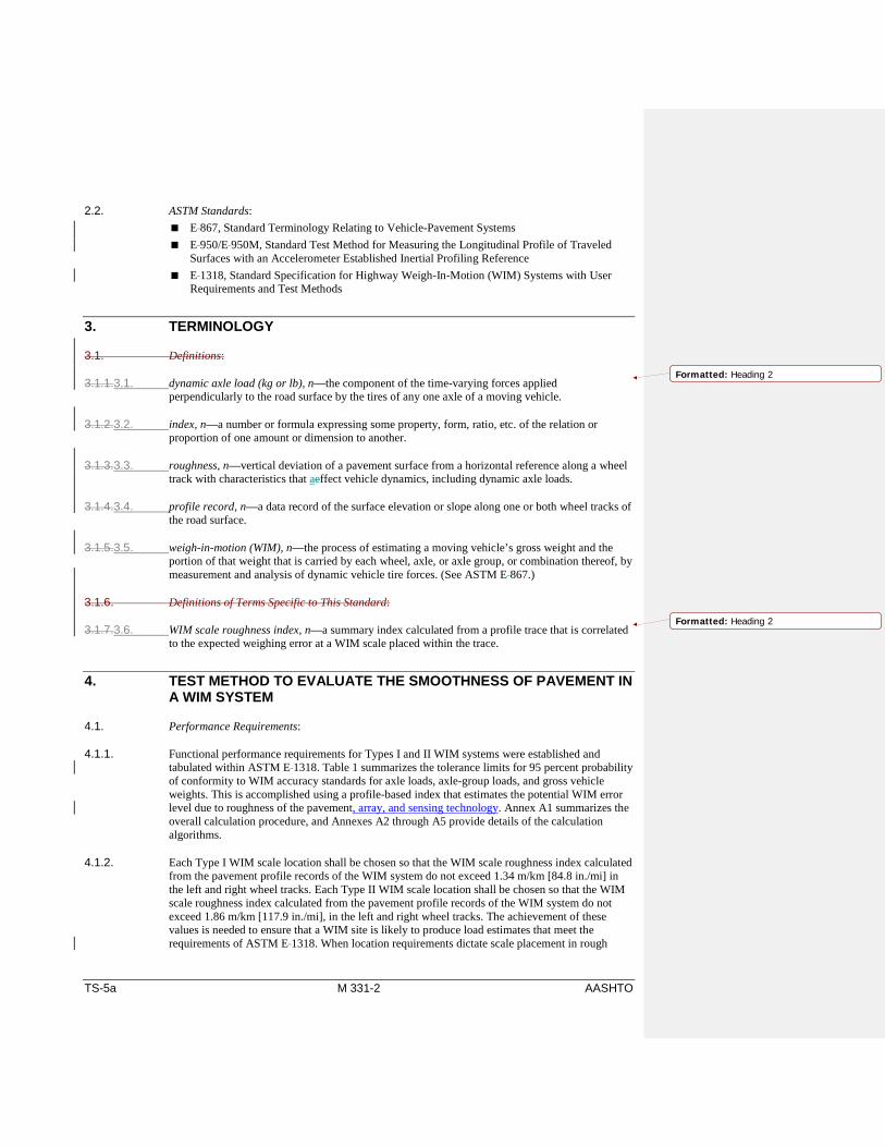
2.2. ASTM Standards: E 867, Standard Terminology Relating to Vehicle-Pavement Systems E 950/E 950M, Standard Test Method for Measuring the Longitudinal Profile of Traveled

Surfaces with an Accelerometer Established Inertial Profiling Reference E 1318, Standard Specification for Highway Weigh-In-Motion (WIM) Systems with User

Requirements and Test Methods

3. TERMINOLOGY

3.1. Definitions:

3.1.1.3.1. dynamic axle load (kg or lb), n—the component of the time-varying forces applied perpendicularly to the road surface by the tires of any one axle of a moving vehicle.

3.1.2.3.2. index, n—a number or formula expressing some property, form, ratio, etc. of the relation or proportion of one amount or dimension to another.

3.1.3.3.3. roughness, n—vertical deviation of a pavement surface from a horizontal reference along a wheel track with characteristics that aeffect vehicle dynamics, including dynamic axle loads.

3.1.4.3.4. profile record, n—a data record of the surface elevation or slope along one or both wheel tracks of the road surface.

3.1.5.3.5. weigh-in-motion (WIM), n—the process of estimating a moving vehicle’s gross weight and the portion of that weight that is carried by each wheel, axle, or axle group, or combination thereof, by measurement and analysis of dynamic vehicle tire forces. (See ASTM E 867.)

3.1.6. Definitions of Terms Specific to This Standard:

3.1.7.3.6. WIM scale roughness index, n—a summary index calculated from a profile trace that is correlated to the expected weighing error at a WIM scale placed within the trace.

4. TEST METHOD TO EVALUATE THE SMOOTHNESS OF PAVEMENT IN A WIM SYSTEM

4.1. Performance Requirements:

4.1.1. Functional performance requirements for Types I and II WIM systems were established and tabulated within ASTM E 1318. Table 1 summarizes the tolerance limits for 95 percent probability of conformity to WIM accuracy standards for axle loads, axle-group loads, and gross vehicle weights. This is accomplished using a profile-based index that estimates the potential WIM error level due to roughness of the pavement, array, and sensing technology. Annex A1 summarizes the overall calculation procedure, and Annexes A2 through A5 provide details of the calculation algorithms.

4.1.2. Each Type I WIM scale location shall be chosen so that the WIM scale roughness index calculated from the pavement profile records of the WIM system do not exceed 1.34 m/km [84.8 in./mi] in the left and right wheel tracks. Each Type II WIM scale location shall be chosen so that the WIM scale roughness index calculated from the pavement profile records of the WIM system do not exceed 1.86 m/km [117.9 in./mi], in the left and right wheel tracks. The achievement of these values is needed to ensure that a WIM site is likely to produce load estimates that meet the requirements of ASTM E 1318. When location requirements dictate scale placement in rough

Formatted: Heading 2

Formatted: Heading 2


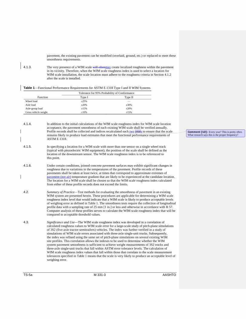
pavement, the existing pavement can be modified (overlaid, ground, etc.) or replaced to meet these smoothness requirements.

4.1.3. The very presence of a WIM scale will oftenmay create localized roughness within the pavement in its vicinity. Therefore, when the WIM scale roughness index is used to select a location for WIM scale installation, the scale location must adhere to the roughness criteria in Section 4.1.2 after the scale is installed.

Table 1—Functional Performance Requirements for ASTM E 1318 Type I and II WIM Systems

Function Tolerance for 95% Probability of Conformance

Type I Type II Wheel load ±25% — Axle load ±20% ±30% Axle-group load ±15% ±20% Gross vehicle weight ±10% ±15%

4.1.4. In addition to the initial calculations of the WIM scale roughness index for WIM scale location acceptance, the pavement smoothness of each existing WIM scale shall be verified annually. Profile records shall be collected and indices recalculated each two years to ensure that the scale remains likely to produce load estimates that meet the functional performance requirements of ASTM E 1318.

4.1.5. In specifying a location for a WIM scale with more than one sensor on a single wheel track (typical with piezoelectric WIM equipment), the position of the scale shall be defined as the location of the downstream sensor. The WIM scale roughness index is to be referenced to this point.

4.1.6. Under certain conditions, jointed concrete pavement surfaces may exhibit significant changes in roughness due to variations in the temperatures of the pavement. Profile records of these pavements shall be taken at least twice, at times that correspond to approximate extremes of pavement (not air) temperature gradient that are likely to be experienced at the candidate location. The location for a WIM scale shall be chosen so that the WIM scale roughness index calculated from either of these profile records does not exceed the limits.

4.2. Summary of Practice—Test methods for evaluating the smoothness of pavement in an existing WIM system are presented herein. These procedures are applicable for determining a WIM scale roughness index level that would indicate that a WIM scale is likely to produce acceptable levels of weighing error as defined in Table 1. The smoothness tests require the collection of longitudinal profile data with a sampling rate of 25 mm [1 in.] or less and otherwise in accordance with R 57. Computer analysis of these profiles serves to calculate the WIM scale roughness index that will be compared to acceptable threshold values.

4.3. Significance and Use—The WIM scale roughness index was developed in a correlation of calculated roughness values to WIM scale error for a large-scale study of pitch-plane simulations of 3S2 (five-axle tractor-semitrailers) vehicles. The index was further verified in a study of simulations of WIM scale errors associated with three-axle single-unit trucks. Subsequently, the index was refined using the same set of pitch-plane simulations on several existing WIM site profiles. This correlation allows the indexes to be used to determine whether the WIM system pavement smoothness is sufficient to achieve weight measurements of 3S2 trucks and three-axle single-unit trucks that fall within ASTM error tolerance levels. The calculation of WIM scale roughness index values that fall within those that correlate to the scale measurement tolerances specified in Table 1 means that the scale is very likely to produce an acceptable level of weighing error.

Comment [U2]: Every year? This is pretty often. What research says this is the proper frequency?


4.4. Procedure:

4.4.1. Profile Records—Obtain profile records of both left and right wheel paths according to the procedures outlined in R 57 using a 25-mm [1-in.] or smaller longitudinal sampling and reporting interval. These records should begin at least 122 m [400 ft] prior to the WIM scale sensor and extend to 61 m [200 ft] after the scale sensor or in accordance with R 57. For WIM scales that are comprised of two or more sensors, the location of the scale will be defined as the location of the downstream sensor. Record the WIM scale location as an Intermediate Feature Location Marker within the profile record as per Section 6.3.4 of ASTM E 950/E 950M. Obtain a total of three records. Compare the outputs for each, and evaluate each for equipment-related spikes. Continue collecting profile records until the operator is satisfied that at least one error-free record has been obtained. Note 1: It should be noted that spacing of sensors, type of sensor technology and processing methods of such sensors also have an impact on the performance of the WIM system in addition to the pavement smoothness.

4.4.2. Calculation of Indexes—A complete description of the procedure to calculate the WIM scale roughness index is described in Annex A1—Computation of the WIM Scale Roughness Index. The procedure has been coded within the Optimal WIM Locator (OWL) within the Profile Viewer and Analysis (ProVAL) software programProVAL. ProVAL was developed for the Federal Highway Administration, which can be used to import, display, and analyze the characteristics of pavement profiles from many different sources. This nonproprietary software, which is available on the web, performs the computations from Annex A1 with either R 57 or ERD text file versions of the profile records from any longitudinal profiler as inputs.

4.4.3. Although including pavement features located outside the range of sensitivity of the WIM scale, roughness index does not improve its predictive ability, the criteria might fail to screen out WIM sites with a major disturbance just beyond its range if the rest of the pavement is not as rough. Although this is unlikely to occur in practice, a useful way to protect against very rough pavement features that are not captured by the index at the scale location is to inspect the value of WIM roughness index for 40 m [131 ft] upstream of the scale to ensure that it does not exceed the threshold over this range.

4.5. Interpretation of Results—Lower threshold values of WIM roughness index are those below which a WIM system is very likely to produce an acceptable level of weighing error. The upper threshold value of the index is that above which a WIM system is very likely to produce an unacceptable level of weighing error. Threshold values for the index for Types I and II WIM scales are tabulated in Table 2 and Table 3, respectively.

Table 2—WIM Roughness Index Thresholds for Type I WIM

Lower Threshold, m/km [in./mi] Upper Threshold, m/km [in./mi] 1.34 [84.8] 2.70 [171.1]

Table 3—WIM Roughness Index Thresholds for Type II WIM Lower Threshold, m/km [in./mi] Upper Threshold, m/km [in./mi]

1.86 [117.9] 3.75 [237.7]

4.6. Precision and Bias—This is a test method that produces pass or fail results. The precision of the test is related to the degree of correlation between calculated index values and errors in measured values of tandem axle and gross vehicle weights. Since these relationships exhibited some scatter in a simulation study, conservative values for index cutoff values were chosen such that there was 95 percent confidence that a scale that met the index criteria would produce levels of weighing error that meet the ASTM E 1318 standards in the study.

Comment [U3]: Recommend removing all references to Lower Thresholds and leave only Upper Thresholds since only the upper values matter in the evaluation.


5. TEST METHOD TO EVALUATE THE SMOOTHNESS OF PAVEMENT TO DETERMINE THE OPTIMAL WIM SYSTEM LOCATION

5.1. Summary of Test Method—A test method for determining the optimal position for a WIM scale within a limited site is presented herein. The procedures are applicable for determining a precise placement of a WIM scale within the linear distance covered by a profiler record that will result in minimum WIM scale roughness index levels. The smoothness tests require the collection of longitudinal profile data with a sampling rate of 25 mm [1 in.] or less and otherwise in accordance with R 57 according to the procedures in ASTM E 950/E 950M. Computer analysis of these profiles at varying longitudinal scale placements serves to place the WIM scale in a location that will minimize the WIM scale roughness index. Comparison of these values with acceptable threshold values will indicate whether the site is suitable. To protect against very rough pavement features that are not captured by the index at the scale location, inspect the value of the index for 40 m [131 ft] upstream of the scale to ensure that it does not exceed the lower threshold over this range.

5.2. Significance and Use—A correlation of has been established between calculated WIM scale roughness index values to and WIM scale error was conducted for a large-scale study of pitch-plane simulations of 3S2 (five-axle tractor-semitrailers) vehicles. This correlation allows the index to be used to determine whether the WIM system pavement smoothness is sufficient to achieve weight measurements of 3S2 trucks and three-axle single-unit trucks that fall within ASTM error tolerance levels. The calculation of WIM scale roughness index for each candidate scale location within a profile record may be used to determine the correct positioning of a scale to maximize its likelihood of producing acceptable levels of weighing error as outlined in Table 1.

5.3. Test Methods:

5.3.1. Profile Records—Obtain profile records of both left and right wheel paths according to the procedures outlined in R 57 using a 25-mm [1-in.] or smaller longitudinal sampling interval. These records shall meet the R 56 requirements for slope profile measured in the waveband specified for the WIM scale roughness index and should cover the entire longitudinal extent of roadway to be considered for the WIM scale placement. Obtain a total of three records, compare the outputs for each, and evaluate each for equipment-related spikes. Continue collecting profile records until the operator is satisfied that at least one error-free record has been obtained.

5.3.2. Calculation of Indexes—A complete description of the procedure to calculate the WIM scale roughness index is described in Annex A1—Computation of the WIM Scale Roughness Index. The procedure has been coded within the Optimal WIM Locator (OWL) in the Profile Viewer and Analysis (ProVAL) software program. ProVAL was developed for the Federal Highway Administration, which can be used to import, display, and analyze the characteristics of pavement profiles from many different sourceswithin ProVAL. This nonproprietary software, which is available on the web, performs the computations from Annex A1 with either R 57 or ERD text file versions of the profile records from any longitudinal profiler as inputs.

5.4. Interpretation of Results—Lower-threshold values of the WIM scale roughness index is that below which a WIM site is very likely to produce an acceptable level of weighing error. The upper threshold value is that above which a WIM site is very likely to produce an unacceptable level of weighing error. Threshold values for the index for Types I and II WIM scales are tabulated in Table 2 and Table 3, respectively. The calculated values that are above the upper threshold value indicate that a WIM site is very likely to produce an unacceptable level of weighing error. A location shall be chosen that will result in acceptable index values below the upper threshold. An acceptable index value is required for a minimum of 40 m [131 ft] prior to the chosen location.

5.5. Precision and Bias—See Section 4.6.


6. REFERENCES

6.1. AASHTO M 328, Standard Specification for Inertial Profiler.

6.2. ASTM E 1170, Standard Practices for Simulating Vehicular Response to Longitudinal Profiles of Traveled Surfaces.

6.3. ASTM E 1364, Standard Test Method for Measuring Road Roughness by Static Level Method.

6.4. FHWA. Traffic Monitoring Guide, Fourth Edition. U.S. Department of Transportation, Federal Highway Administration, Office of Highway Policy Information Management, Washington, DC, January September 20012013. http://www.fhwa.dot.gov/policyinformation/tmguide/tmg_fhwa_pl_13_015.pdf

6.5. FHWA. Pavement Smoothness Specifications for LTPP WIM Locations, Draft. Federal Highway Administration, Office of Infrastructure Research, Development, and Technology, McLean, VA, January 2002.

6.5. NCHRP Synthesis 20-05/Topic 38-10. High Speed Weigh-in-Motion System Calibration Practices http://onlinepubs.trb.org/onlinepubs/nchrp/nchrp_syn_386.pdf.

6.6. FHWA. A Program Guide to WIM Smoothness Index Software. Federal Highway Administration, Office of Infrastructure Research, Development, and Technology, McLean, VA, 2005.

6.7. Karamihas, Steven M. and Thomas D. Gillespie. Smoothness Criteria for WIM Scale Approaches. University of Michigan Transportation Research Institute, Ann Arbor, MI, September 2002.

6.8. Karamihas, Steven M. and Thomas D. Gillespie. Advancement of Smoothness Criteria for WIM Scale Approaches—Final Report. University of Michigan Transportation Research Institute, Ann Arbor, MI, April 2004.

ANNEXES

(Mandatory Information)

A1. COMPUTATION OF THE WIM SCALE ROUGHNESS INDEX

A1.1. This Annex describes the procedure for producing a plot of WIM Scale Roughness Index versus longitudinal distance from a measured longitudinal profile.

A1.2. Step 1: Apply a longitudinal bridging filter as specified in Annex A2.

A1.3. Step 2: Apply a band-pass filter as specified in Annex A3. Use a cutoff wavelength for the low-pass filter of 1.07 m [3.5 ft]. Use a cutoff wavelength for the high-pass filter of 16.46 m [54 ft].

A1.4. Step 3: Rectify the filtered slope profile as specified in Annex A4.

A1.5. Step 4: Apply a shroud to the signal as specified in Annex A5. The resulting signal provides the WIM Scale Roughness Index versus location.

A2. BRIDGING FILTER

Formatted: Normal

Comment [ajm4]: AASHTO – please adjust section numbering

http://onlinepubs.trb.org/onlinepubs/nchrp/nchrp_syn_386.pdf


A2.1. Apply a low-pass bridging filter to the profile, unless a low-pass filter with a base length or a similar influence on the frequency content was applied before recording the profile.

A2.2. The bridging filter emulates tire behavior by assuming that the positive (upward) content in the profile over the tire contact patch will penetrate into the tread by a consistent depth DB, but that negative (downward) content has no influence.

A2.3. For each data point in the raw profile PR (i), seek a value for the bridged profile P(i) as follows:

Step 1: Set the desired depth. A2.3.1.D = DB (A2.1)

Step 2: Assume a value for the bridged profile. A2.3.2.P(i) = PR(i) – D (A2.2)

Step 3: Calculate the average depth of penetration of the raw profile above the bridged profile. A2.3.3.

1 max(0, ( ) ( ))2 1

B

B

i I

A Ri IB

D P i P iI

+

−

= −+ ∑ 1 max(0, ( ) ( ))

2 1

B

B

i I

A Ri IB

D P i P iI

+

−

= −+ ∑ (A2.3)

NINT ( / 2)BI B= (A2.4)

NINT ( / 2)BI B= (A2.4)

1 max(0, ( ) ( ))2 1

B

B

i I

A Ri IB

D P i P iI

+

−

= −+ ∑ 1 max(0, ( ) ( ))

2 1

B

B

i I

A Ri IB

D P i P iI

+

−

= −+ ∑ (A2.3)

NINT ( / 2)BI B= NINT ( / 2)BI B= (A2.4)

B is the base length. The function NINT produces the nearest integer of its argument.

Step 4: Test the depth. A2.3.4.

0.001ADD

> (A2.5)

0.001ADD

> (A2.5)

0.001ADD

> 0.001ADD

> (A2.5)

Set D = D – DA and return to Step 1.

Step 5: Shift the profile upward. A2.3.5.P(i) = PR(i) + DB (A2.6)

A2.4. Apply the steps described in Section A2.3 at every point along the profile for a base length (B) of 250 mm [9.84 in.] and a depth (DB) of 1 mm [0.04 in.]. For cases where the sum used in Equation A2.3 would require data that are outside the limits of the raw profile, pad the signal by assuming a constant elevation equal to the appropriate endpoint.

A3. BAND-PASS FILTERING

A3.1. Sixth-Order Butterworth Filter:

Comment [ajm5]: AASHTO – all the following indicated changes in this Annex were somehow done automatically. There are no changes proposed by TS 5a.

Field Code Changed

Field Code Changed

Field Code Changed

Field Code Changed

Field Code Changed

Field Code Changed

Field Code Changed

Field Code Changed


A prefilter shall be applied. An elevation profile for each wheel track is replaced with a slope A3.1.1.profile, obtained point-by-point by subtracting adjacent elevation values and dividing by the sample interval.

An ideal band-pass filter passes some range of frequencies without distortion and suppresses all A3.1.2.other frequencies. A Butterworth filter fulfills these needs to some extent. The exclusion of very short and very long wavelengths minimizes the effects of high-amplitude, short-wavelength change in the profile at the edges of the spatial weighting function. It also prevents absolute elevation or grade from influencing index values by filtering the very-long-wavelength content from within a signal.

The filter described herein is a sixth-order low-pass filter combined with a sixth-order high-pass A3.1.3.filter. Both filters are applied in a cascaded form of a third-order Butterworth filter in the forward and reverse directions. Apply the low-pass filter first, and then apply the high-pass filter.

A typical Butterworth filter produces a phase lag in the conditioned profile. Applying each filter A3.1.4.twice, once in each direction, cancels the lag.

The output of each filter includes an initial transient. This is most evident when the filter is applied A3.1.5.to profiles with a significant slope at the leading end. However, the severity of the initial transient depends on the sequence of the filter components. The filters are applied in the following sequence: (1) first-order, forward direction, (2) second-order, reverse direction, (3) first-order, reverse direction, and (4) second-order, forward direction.

Formatted: Normal


A3.1.5.

A3.2. Filtering Constants:

To get the appropriate gain reduction at a desired wavelength, L, the value of L must be adjusted A3.2.1.as follows for the low-pass filter:

( )(1/6)2 1L L′= − × (A3.1)

( )(1/6)2 1L L′= − × ( )(1/6)

2 1L L′= − × (A3.1)

A similar adjustment is required for the high-pass filter:

( ) (1/6)2 1L L

−′= − × (A3.2)

( ) (1/6)2 1L L

−′= − × (A3.2)

( ) (1/6)2 1L L

−′= − × ( ) (1/6)

2 1L L−

′= − × (A3.2)

Apply these adjustments in the following constant, which appears in the formulas for filtering A3.2.2.constants:

cot( / )c x L= × ∆π (A3.3)

cot( / )c x L= × ∆π (A3.3)

cot( / )c x L= × ∆π cot( / )c x L= × ∆π (A3.3)

For low-pass filtering, use the following constants: A3.2.3.

10 11 10 111, 1 , 1N N D c D c= = = + = − 10 11 10 111, 1 , 1N N D c D c= = = + = − (A3.4)

20 22 212 2 2

20 21 22

1, 2

1 , 2 2 , 1

N N N

D c c D c D c c

= = =

= + + = − = − +

10 11 10 111, 1 , 1N N D c D c= = = + = − 10 11 10 111, 1 , 1N N D c D c= = = + = − (A3.4)

20 22 212 2 2

20 21 22

1, 2

1 , 2 2 , 1

N N N

D c c D c D c c

= = =

= + + = − = − +

20 22 212 2 2

20 21 22

1, 2

1 , 2 2 , 1

N N N

D c c D c D c c

= = =

= + + = − = − +

For high-pass filtering, use the following constants: A3.2.4.

10 11 10 11, , 1 , 1N c N c D c D c= = − = + = −

2 220 22 21

2 2 220 21 22

, 2

1 , 2 2 , 1

N N c N c

D c c D c D c c

= = =

= + + = − = − +10 11 10 11, , 1 , 1N c N c D c D c= = − = + = −

2 220 22 21

2 2 220 21 22

, 2

1 , 2 2 , 1

N N c N c

D c c D c D c c

= = =

= + + = − = − +10 11 10 11, , 1 , 1N c N c D c D c= = − = + = −

Formatted: Normal

Field Code Changed

Field Code Changed

Field Code Changed

Field Code Changed

Field Code Changed

Field Code Changed

Field Code Changed

Field Code Changed

Field Code Changed

Field Code Changed

Field Code Changed

Field Code Changed

Field Code Changed

Field Code Changed

Field Code Changed


2 220 22 21

2 2 220 21 22

, 2

1 , 2 2 , 1

N N c N c

D c c D c D c c

= = =

= + + = − = − + (A3.5)

A3.3. Numerical Filtering Procedure:

Step 1: First-order, forward direction: A3.3.1.

A3.3.1.1. For a given input profile (P) with NS samples, the first-order filter applied in the forward direction produces the output (F1) as follows:

1 10 11 11 110

1 ( ( ) ( 1) ( 1))F N P i N P i D F iD

= + − − − (A3.6)

1 10 11 11 110

1 ( ( ) ( 1) ( 1))F N P i N P i D F iD

= + − − − 1 10 11 11 110

1 ( ( ) ( 1) ( 1))F N P i N P i D F iD

= + − − −

1 10 11 11 110

1 ( ( ) ( 1) ( 1))F N P i N P i D F iD

= + − − − (A3.6)

A3.3.1.2. To initialize the low-pass filter, set F1 (1) to P(1).

A3.3.1.3. To initialize the high-pass filter, set F1 (1) to 0.

A3.3.1.4. After initialization, apply Equation A3.6 by stepping the index value (i) through the range from 2 to NS.

Step 2: Second-order, reverse direction: A3.3.2.

A3.3.2.1. The second-order (complement) reverse filter transforms F1 to the intermediate signal F2 as follows:

2 20 1 21 1 22 1 21 2 22 220

1( ) ( ( ) ( 1) ( 2) ( 1) ( 2))F i N F i N F i N F i D F i D F iD

= + + + + − + − + (A3.7)

2 20 1 21 1 22 1 21 2 22 220


= + + + + − + − + (A3.7)

2 20 1 21 1 22 1 21 2 22 220


= + + + + − + − +

2 20 1 21 1 22 1 21 2 22 220


= + + + + − + − + (A3.7)

A3.3.2.2. To initialize the low-pass filter, set F2 (NS) to F1 (NS), and then apply:

2 10 1 11 11 110

1( 1) ( ( 1) ( ) ( ))S S SF N N F N N D F ND

− = − + − (A3.8)

2 10 1 11 11 110

1( 1) ( ( 1) ( ) ( ))S S SF N N F N N D F ND

− = − + − (A3.8)

Field Code Changed

Field Code Changed

Field Code Changed

Field Code Changed

Field Code Changed

Field Code Changed

Field Code Changed

Field Code Changed

Field Code Changed


2 10 1 11 11 110

1( 1) ( ( 1) ( ) ( ))S S SF N N F N N D F ND

− = − + −

2 10 1 11 11 110

1( 1) ( ( 1) ( ) ( ))S S SF N N F N N D F ND

− = − + − (A3.8)

A3.3.2.3. To initialize the high-pass filter, set F2 (NS) to 0, and then apply:

2 10 1 11 110

1( 1) ( ( 1) ( ))S S SF N N F N N F ND

− = − + (A3.9)

2 10 1 11 110

1( 1) ( ( 1) ( ))S S SF N N F N N F ND

− = − + 2 10 1 11 110

1( 1) ( ( 1) ( ))S S SF N N F N N F ND

− = − +

2 10 1 11 110

1( 1) ( ( 1) ( ))S S SF N N F N N F ND

− = − + (A3.9)

A3.3.2.4. After initialization, apply Equation A3.7 by stepping the index value (i) through the range in reverse from NS – 2 to 1.

Step 3: First-order, reverse direction: A3.3.3.

A3.3.3.1. The first-order reverse filter transforms F2 to the intermediate signal F3 as follows:

3 10 2 11 2 11 310

1( ) ( ( ) ( 1) ( 1))F i N F i N F i D F iD

= + + − + (A3.10)

3 10 2 11 2 11 310

1( ) ( ( ) ( 1) ( 1))F i N F i N F i D F iD

= + + − + 3 10 2 11 2 11 310

1( ) ( ( ) ( 1) ( 1))F i N F i N F i D F iD

= + + − +

3 10 2 11 2 11 310

1( ) ( ( ) ( 1) ( 1))F i N F i N F i D F iD

= + + − + (A3.10)

A3.3.3.2. To initialize the low-pass filter, set F3 (NS) to F2 (NS).

A3.3.3.3. To initialize the high-pass filter, set F3 (NS) to 0.

A3.3.3.4. After initialization, apply Equation A3.10 by stepping the index value (i) through the range in reverse from NS – 1 to 1.

Step 4: Second-order, forward direction: A3.3.4.

A3.3.4.1. The second-order (complement) filter transforms F3 to the final signal F4 as follows:

4 20 3 21 3 22 3 21 4 22 420


= + − + − − − − − (A3.11)

4 20 3 21 3 22 3 21 4 22 420


= + − + − − − − −

4 20 3 21 3 22 3 21 4 22 420


= + − + − − − − −

4 20 3 21 3 22 3 21 4 22 420


= + − + − − − − − (A3.11)

Field Code Changed

Field Code Changed

Field Code Changed

Field Code Changed

Field Code Changed

Field Code Changed

Field Code Changed

Field Code Changed

Field Code Changed

Field Code Changed


A3.3.4.2. To initialize the low-pass filter, set F4(1) to F3(1), and then apply:

4 10 3 11 11 310

1(2) ( (2) ( ) (1))F N F N D FD

= + − (A3.12)

4 10 3 11 11 310

1(2) ( (2) ( ) (1))F N F N D FD

= + − 4 10 3 11 11 310

1(2) ( (2) ( ) (1))F N F N D FD

= + −

4 10 3 11 11 310

1(2) ( (2) ( ) (1))F N F N D FD

= + − (A3.12)

A3.3.4.3. To initialize the high-pass filter, set F4(1) to 0, and then apply:

4 10 3 11 310

1(2) ( (2) (1))F N F N FD

= + (A3.13)

4 10 3 11 310

1(2) ( (2) (1))F N F N FD

= + 4 10 3 11 310

1(2) ( (2) (1))F N F N FD

= +

4 10 3 11 310

1(2) ( (2) (1))F N F N FD

= + (A3.13)

A3.3.4.4. After initialization, apply Equation A3.11 by stepping the index value (i) through the range from 3 to NS.

A4. CONTINUOUS REPORTING

A4.1. Transform the band-pass–filtered profile to a continuous report of the WIM scale roughness index.

A4.1. Rectify the signal by replacing every value in it by its absolute value. A4.1.1.

Field Code Changed

Field Code Changed

Field Code Changed

Field Code Changed

Field Code Changed

Field Code Changed

Formatted: Heading 3A


A4.1.1. Rectify the signal by replacing every value in it by its absolute value.

( ) ( ) , 1, SF i F i i N= = (A4.1) A4.1.2.

( ) ( ) , 1, SF i F i i N= = (A4.1) A4.1.3.

( ) ( ) , 1, SF i F i i N= = ( ) ( ) , 1, SF i F i i N= = (A4.1) A4.1.4.

Formatted: Heading 3A, Outline numbered +Level: 3 + Numbering Style: 1, 2, 3, … + Startat: 1 + Alignment: Left + Aligned at: 0" + Tabafter: 1" + Indent at: 1"

Field Code Changed

Field Code Changed

Formatted: Heading 3A

Field Code Changed


A5. SHROUD

A5.1. To help avoid underestimating WIM scale error near areas of localized roughness, a shroud is placed over the continuous report to increase the WIM scale roughness index near hot spots.

A5.2. The aft shroud is based on exponential decay from localized peaks with a preset distance constant of 15.24 m [50 ft] for hot spots upstream of a point of interest. To apply the shroud, step through the signal from the start (i + IB) to the end (NS – IB).

For each point in the signal, search the points upstream (i.e., step through possible values of j from A5.2.1.1 to i –1) until the following condition is satisfied:

/( ) ( ) axjF i F i j e−∆< − × τ (A5.1)

/( ) ( ) axjF i F i j e−∆< − × τ (A5.1)

/( ) ( ) axjF i F i j e−∆< − × τ /( ) ( ) axjF i F i j e−∆< − × τ (A5.1)

Where ∆x is the longitudinal distance interval and τa is the distance constant. For the first value of j in which Equation A5.1 is satisfied, replace F(i) as described in Equation A5.2, and move on to the next point in the signal. (Once a “hit” is found, it is not necessary to continue through any more possible values of j.)

/( ) ( ) axjF i F i j e−∆= − × τ (A5.2)

/( ) ( ) axjF i F i j e−∆= − × τ (A5.2)

/( ) ( ) axjF i F i j e−∆= − × τ /( ) ( ) axjF i F i j e−∆= − × τ (A5.2)

A5.3. The forward shroud is based on exponential decay from localized peaks with a preset distance constant of 1.524 m [5 ft] for hot spots downstream of a point of interest. To apply the shroud, step through the signal from the end (NS – IB) to the start (I + IB).

For each point in the signal, search the points downstream (i.e., step through possible values of j A5.3.1.from 1 to NS – IB – i) until the following condition is satisfied:

/( ) ( ) fxjF i F i j e−∆< + × τ (A5.3)

/( ) ( ) fxjF i F i j e−∆< + × τ (A5.3)

/( ) ( ) fxjF i F i j e−∆< + × τ /( ) ( ) fxjF i F i j e−∆< + × τ (A5.3)

Where ∆x is the longitudinal distance interval and τf is the distance constant. For the first value of j in which Equation A5.3 is satisfied, replace F(i) as described in Equation A5.4, and move on to the previous point in the signal. (Once a “hit” is found, it is not necessary to continue through any more possible values of j.)

/( ) ( ) fxjF i F i j e−∆= + × τ /( ) ( ) fxjF i F i j e−∆= + × τ (A5.4)

/( ) ( ) fxjF i F i j e−∆= + × τ /( ) ( ) fxjF i F i j e−∆= + × τ (A5.4)

Formatted: Normal

Field Code Changed

Field Code Changed

Field Code Changed

Field Code Changed

Field Code Changed

Field Code Changed

Field Code Changed

Field Code Changed

Field Code Changed

Field Code Changed

Field Code Changed


1 Formerly AASHTO Provisional Standard MP 14. First published as a full standard in 2013.

aashto subcommittee on materials · approve august 2015 technical section annual meeting minutes:...

Documents