aalborg university - inpe university institute of electronic systems d fredrik bajers vej 7 dk-9220...
TRANSCRIPT


Aalborg University
Institute of Electronic Systems dFredrik Bajers Vej 7 DK-9220 Aalborg Øst Telephone +45 96 35 87 00
Title: Attitude Control System for AAUSAT-II
Theme: Modelling and Control
Project period: February 2nd 2005 - May 30th 2005
Project group:
IAS8-05GR834
Group members:
Bo Ørsted Andresen
Claus Grøn
Rasmus Hviid Knudsen
Claus Nielsen
Kresten Kjær Sørensen
Dan Taagaard
Supervisor:
Dan Bhanderi
Publications: 9Pages: 113Finished: May 30th 2005
AbstractThis report documents the work of group05GR834, concerning the development of an atti-tude control system for the AAUSAT-II satellite.A model of the satellite kinematics and dynamicshas been implemented in a simulation environ-ment containing relevant disturbances.The attitude control system features both magne-torquers and momentum wheels to facilitate threeaxes control of the satellite and by the means ofmagnetic and mechanical actuation, the satellite isable to detumble and do slew manoeuvres.To detumble the satellite, using only magnetic ac-tuation, a controller based on the B-dot algorithmhas been designed. For pointing purposes the at-titude control system features a control supervi-sor to manage the attitude controllers. The atti-tude controllers consist of an optimal controllerfor controlling the momentum wheels and a desat-uration controller to keep the momentum wheelsfrom reaching their saturation limits.The controllers have been tested in the simula-tion environment with successful results. The B-dot controller performs robustly and meets the de-mands, hence it is ready for implementation onthe satellite. Simulations of the attitude control-lers show that they meet the demands as well andenables the satellite to perform slew manoeuvresand maintain a given attitude.


Preface
This report documents the project of developing the attitude control system for AAUSAT-II. The project ismade on 8th semester in the specialization of Intelligent Autonomous Systems at the Department of ControlEngineering, Aalborg University.
The project was initiated February 2nd 2005 and finished May 30th 2005.
Throughout the report figures, tables and equations are numbered consecutively according to the chapters.Citation numbers are referring to the bibliography at page 79, e.g. [Wertz, page 571] is referring to page 571in Spacecraft Attitude Determination and Control by James R. Wertz. Equations are referred to in parenthesese.g. (1.4) refers to Equation 1.4 on page 14.
The project is closely connected to the AAUSAT-II attitude determination system, hence Chapters 1, 2 andparts of the appendices have been written in collaboration with group 05GR833, who are developing theattitude determination system for AAUSAT-II. The project is a continuation of an earlier project concerningthe attitude control system for AAUSAT-II made by group 04GR830a.
Simulation files, data sheets and other relevant documentation is available from the enclosed CD-ROM.
Aalborg University, May 30th 2005
—————————————————— —————————————————–
Bo Ørsted Andresen Claus Grøn
—————————————————— —————————————————–
Rasmus Hviid Knudsen Claus Nielsen
—————————————————— ——————————————————
Kresten Kjær Sørensen Dan Taagaard
III

Table of Contents
1 The AAUSAT-II Satellite 81.1 Background . . . . . . . . . . . . . . . . . . . . . . . . . . . . . . . . . . . . . . . . . . . . . . . . 81.2 Mission Objectives for AAUSAT-II . . . . . . . . . . . . . . . . . . . . . . . . . . . . . . . . . . . 81.3 AAUSAT-II Subsystems . . . . . . . . . . . . . . . . . . . . . . . . . . . . . . . . . . . . . . . . . 91.4 Satellite Modes . . . . . . . . . . . . . . . . . . . . . . . . . . . . . . . . . . . . . . . . . . . . . . 111.5 Requirements for the Attitude Determination and Control System . . . . . . . . . . . . . . . . 12
2 Modelling 182.1 Coordinate Systems . . . . . . . . . . . . . . . . . . . . . . . . . . . . . . . . . . . . . . . . . . . 182.2 Ephemeris . . . . . . . . . . . . . . . . . . . . . . . . . . . . . . . . . . . . . . . . . . . . . . . . . 252.3 Disturbance Modelling . . . . . . . . . . . . . . . . . . . . . . . . . . . . . . . . . . . . . . . . . 282.4 Earth Albedo . . . . . . . . . . . . . . . . . . . . . . . . . . . . . . . . . . . . . . . . . . . . . . . 322.5 Orbit Propagator . . . . . . . . . . . . . . . . . . . . . . . . . . . . . . . . . . . . . . . . . . . . . 342.6 Magnetic Field Model . . . . . . . . . . . . . . . . . . . . . . . . . . . . . . . . . . . . . . . . . . 342.7 Satellite Dynamics and Kinematics . . . . . . . . . . . . . . . . . . . . . . . . . . . . . . . . . . . 352.8 Transducers . . . . . . . . . . . . . . . . . . . . . . . . . . . . . . . . . . . . . . . . . . . . . . . . 422.9 Actuator Modelling . . . . . . . . . . . . . . . . . . . . . . . . . . . . . . . . . . . . . . . . . . . 42
3 Controllers 513.1 Control Strategy . . . . . . . . . . . . . . . . . . . . . . . . . . . . . . . . . . . . . . . . . . . . . 513.2 Control Supervisor . . . . . . . . . . . . . . . . . . . . . . . . . . . . . . . . . . . . . . . . . . . . 523.3 Controllability . . . . . . . . . . . . . . . . . . . . . . . . . . . . . . . . . . . . . . . . . . . . . . 553.4 Detumbling Controller . . . . . . . . . . . . . . . . . . . . . . . . . . . . . . . . . . . . . . . . . 563.5 Optimal Controller for Attitude Control . . . . . . . . . . . . . . . . . . . . . . . . . . . . . . . . 613.6 Desaturation Controller . . . . . . . . . . . . . . . . . . . . . . . . . . . . . . . . . . . . . . . . . 74
4 Conclusion 784.1 Future Work . . . . . . . . . . . . . . . . . . . . . . . . . . . . . . . . . . . . . . . . . . . . . . . . 79
Bibliography 81
A Quaternions 82A.1 Quaternion Definitions . . . . . . . . . . . . . . . . . . . . . . . . . . . . . . . . . . . . . . . . . 82A.2 Quaternion Algebra . . . . . . . . . . . . . . . . . . . . . . . . . . . . . . . . . . . . . . . . . . . 83
B Rotations 85B.1 Direction Cosine . . . . . . . . . . . . . . . . . . . . . . . . . . . . . . . . . . . . . . . . . . . . . 85B.2 Euler Angles . . . . . . . . . . . . . . . . . . . . . . . . . . . . . . . . . . . . . . . . . . . . . . . 86B.3 Euler’s Eigenaxis Rotation Theorem . . . . . . . . . . . . . . . . . . . . . . . . . . . . . . . . . . 87B.4 Attitude Matrix and Kinematics . . . . . . . . . . . . . . . . . . . . . . . . . . . . . . . . . . . . 88
C Two Line Elements 91
D Linearization 93D.1 Linearization of the Satellite Kinematic Equation . . . . . . . . . . . . . . . . . . . . . . . . . . 93
IV

TABLE OF CONTENTS
D.2 Linearization of Satellite Dynamic Equation . . . . . . . . . . . . . . . . . . . . . . . . . . . . . 96D.3 Linear Equation for the Satellite Attitude . . . . . . . . . . . . . . . . . . . . . . . . . . . . . . . 97
E Implementation of Simulation 98E.1 Simulation Environment . . . . . . . . . . . . . . . . . . . . . . . . . . . . . . . . . . . . . . . . 98
F Orbit Propagator Accuracy 108
G Magnetic Field Model Accuracy 111
V
Nomenclature
Acronyms
ACS Attitude Control System
ADCS Attitude Determination and Control System
ADS Attitude Determination System
CDH Command and Data Handling
COM Communication system
DCM Direct Cosine Matrix
EPS Electrical Power Supply
GND Ground Station
ICD Interface Control Document
IGRF International Geomagnetic Reference Field
JD Julian Date. The number of days since January 1st, 4713 B.C., at 12.00AM UTC.
LEO Low Earth Orbit
MCC Mission Control Center
MECH Mechanical structure
OBC On-Board Computer
P/L Payload
SGP4 Simplified General Perturbations 4
TLE Two Line Element
Reference Frames
ECI Earth Centered Inertial reference frame. Abbreviated I in equations.
ECEF Earth Centered Earth Fixed reference frame. Abbreviated E in equations.
ORF Orbit Reference Frame. Abbreviated O in equations.
SBRF Satellite Body Reference Frame. Abbreviated S in equations.
CRF Controller Reference Frame. Abbreviated C in equations.
6

Nomenclature
Notation
Vectors, Matrices and Rotations
• Vectors are typed asv
• Unit vectors are typed asu
• Matrices are typed asM
• Identity matrices are typed as1n×n (1)
e.g. a 3×3 identity matrix is written as
13×3 =
1 0 0
0 1 0
0 0 1
• Rotations (quaternions and matrices) are typed with source frame designation (preceding subscript)
and destination frame designation (preceding superscript). E.g.,
IEq, C
I C
IEq is a quaternion describing a rotating from ECEF to ECI and C
I C is a matrix describing a rotatingfrom ECI to CRF.
• Vector and quaternion components are typed as
Evx,Iq1:3
which denotes the component x of the vector v in ECEF, and the components 1 through 3 of the quater-nion q in the ECI frame.
Signals
• Small signals are typed asq
which denotes the small signal quaternion.
• Operating points are typed asq
which denotes the quaternion in the operating point.
7

The AAUSAT-II Satellite 1This chapter describes the mission the AAUSAT-II satellite shall accomplish during the designated time ofoperation. This includes a description of the purpose and functionality of each subsystem on-board thesatellite.
1.1 Background
The AAUSAT-II satellite is a pico satellite which is constructed by students primarily at Aalborg University.The project was initiated in September 2003 and the satellite is expected to be launched in December 2005.Another satellite, AAU CubeSat, has been developed at Aalborg University and was launched in April 2003,and was a great success.
The AAUSAT-II follows the CubeSat concept developed by California Polytechnic State University, San LuisObispo and Space Systems Development Laboratory at Stanford University [CPSU]. This concept allowsthe satellite to have a mass of maximum 1 [kg] and the dimensions of 10 [cm] × 10 [cm] × 10 [cm], hence thename CubeSat. The size constrains the amount of power and space available which entails that low powerconsumption, small volume and low mass are important factors in the design process.
1.2 Mission Objectives for AAUSAT-II
A number of mission objectives have been formulated for the AAUSAT-II project. The mission objectivesare defined in an order, such that the first objective has to be accomplished before trying to accomplish thesecond objective.
1. Education of the students and staff involved with the AAUSAT-II project.The primary mission for the satellite project is to educate the students and the staff working on it.The satellite shall be built by students mostly. Staff related to the project are only meant to act asadvisors and final arbitrators. The purpose of this is to enable the students to make important decisionsbased on their own experience which is an important part of engineering studies, since a satellite is acomplicated system which requires a lot of coordination between all groups working with the project.
2. Communication.In order to ensure the communication with the satellite is functioning, one-way communication isestablished when a basic beacon with the correct syntax is received at the ground station. When two-way communication is established, by sending a command to the satellite and a correct answer corre-sponding to the command, is received from the satellite, the communication objective is fulfilled.
3. Payload.The AAUSAT-II carries a gamma ray burst detector as a payload. The gamma ray burst detector isdeveloped at the Danish National Space Center (DNSC), and is used for measuring the radiation fromgamma bursts in space. This objective is fulfilled when correct and usable data has been received fromthe satellite.
8
1.3. AAUSAT-II SUBSYSTEMS
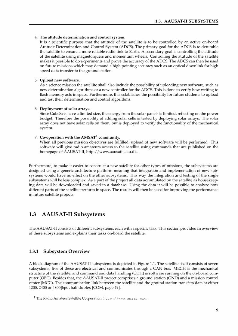
4. The attitude determination and control system.It is a scientific purpose that the attitude of the satellite is to be controlled by an active on-boardAttitude Determination and Control System (ADCS). The primary goal for the ADCS is to detumblethe satellite to ensure a more reliable radio link to Earth. A secondary goal is controlling the attitudeof the satellite using magnetorquers and momentum wheels. Controlling the attitude of the satellitemakes it possible to do experiments and prove the accuracy of the ADCS. The ADCS can then be usedon future missions which may demand a high pointing accuracy such as an optical downlink for highspeed data transfer to the ground station.
5. Upload new software.As a science mission the satellite shall also include the possibility of uploading new software, such asnew determination algorithms or a new controller for the ADCS. This is done to verify how writing toflash memory acts in space. Furthermore, this establishes the possibility for future students to uploadand test their determination and control algorithms.
6. Deployment of solar arrays.Since CubeSats have a limited size, the energy from the solar panels is limited, reflecting on the powerbudget. Therefore the possibility of adding solar cells is tested by deploying solar arrays. The solararray does not have solar cells on them, but is deployed to verify the functionality of the mechanicalsystem.
7. Co-operation with the AMSAT1 community.When all previous mission objectives are fulfilled, upload of new software will be performed. Thissoftware will give radio amateurs access to the satellite using commands that are published on thehomepage of AAUSAT-II, http://www.aausatii.aau.dk.
Furthermore, to make it easier to construct a new satellite for other types of missions, the subsystems aredesigned using a generic architecture platform meaning that integration and implementation of new sub-systems would have no effect on the other subsystems. This way the integration and testing of the singlesubsystems will be less complex. As a part of the project all data accumulated on the satellite as housekeep-ing data will be downloaded and saved in a database. Using the data it will be possible to analyze howdifferent parts of the satellite perform in space. The results will then be used for improving the performancein future satellite projects.
1.3 AAUSAT-II Subsystems
The AAUSAT-II consists of different subsystems, each with a specific task. This section provides an overviewof these subsystems and explains their tasks on-board the satellite.
1.3.1 Subsystem Overview
A block diagram of the AAUSAT-II subsystems is depicted in Figure 1.1. The satellite itself consists of sevensubsystems, five of these are electrical and communicates through a CAN bus. MECH is the mechanicalstructure of the satellite, and command and data handling (CDH) is software running on the on-board com-puter (OBC). Besides that, the AAUSAT-II project comprises a ground station (GND) and a mission controlcenter (MCC). The communication link between the satellite and the ground station transfers data at either1200, 2400 or 4800 [bps], half duplex [COM, page 49].
1 The Radio Amateur Satellite Corporation, http://www.amsat.org.
9

1.3. AAUSAT-II SUBSYSTEMS
P/LEPS
MCCGND
COM
MECH
Earth
Satellite
ADCS
OBC
CDH
Radio Link
AX.25
CAN bus
TCP
Figure 1.1: Block diagram depicting the subsystems in theAAUSAT-II and a conceptual visualization of their respective in-terfaces to other subsystems.
1.3.2 Subsystem Descriptions
MCC (Mission Control Center) is responsible for handling and storing all transmission data from the satel-lite and sending flight plans etc. to the satellite. The MCC provides a user interface and a database tostore housekeeping data from the satellite. The mission control center is furthermore able to controlmultiple ground stations, both the ground station located in Aalborg and a ground station placed atSvalbard in Norway which is currently in the final stages of developement.
GND (Ground Station) is responsible for the communication between the MCC and the satellite. The task ofthe ground station is to track the satellite throughout each pass and adjust the radio frequency, so databetween the satellite and the MCC can be sent and received correctly. Furthermore, the ground stationis designed to be autonomously controlled by the MCC, both for communicating with the AAUSAT-IIsatellite and the ESA SSETI Express satellite2.
COM (Communication System) is designed to function as a pipeline for the communication between theground station and the CDH. COM modulates and sends data from CDH to the ground station. Datareceived from the ground station is demodulated and sent via the CAN bus to the CDH subsystem.
EPS (Electrical Power Supply) is responsible for generating power from the solar cells and storing it in thebatteries in order to be able to deliver continuous power during eclipse and peak demands. The EPSsubsystem also conditions and distributes the power to other satellite subsystems.
ADCS (Attitude Determination and Control System) is responsible for determining and controlling the at-titude of the satellite. This primarily implies detumbling and stabilization of the satellite.
P/L (Payload) consists of a gamma ray burst detector. The gamma ray burst detector is a newly developeddetector crystal supplied by Danish National Space Center.
OBC (On-Board Computer) is the main computer on the satellite. The CDH subsystem software is executedon the OBC. The OBC subsystem also provides processing facilities for other satellite subsystems.
2http://sseti.gte.tuwien.ac.at/WSW4/express1.htm
10

1.4. SATELLITE MODES
CDH (Command and Data Handling) is implemented as software running on the OBC. The CDH subsys-tem is responsible for maintaining the flight plan, accumulating housekeeping data, managing thesubsystems and controlling the communication with the ground station.
MECH (Mechanical Structure) provides the physical satellite frame structure and casing in which the othersatellite subsystems are mounted. Besides the satellite frame, also an additional solar cell array isdesigned to be mounted on the satellite frame.
The satellite is an intelligent autonomous system which interacts on tele commands sent from the MCC usingthe ground station. The communication path is illustrated in Figure 1.2. A tele command is transmittedthrough the ground station and received by the COM system. The communication system then passes thetele command on to the CDH system which decodes and executes the command. It is not possible to send acommand directly through the communication system to a specific subsystem. All tele commands is directedthrough the CDH system.
GND
TCP
Radio
Link
CAN busCAN bus
CAN bus
COM CDH ADCS
EPS
P/L
MCC
Figure 1.2: The communication path for the AAUSAT-II.
1.3.3 Description of the Attitude Determination and Control System
During development of the AAUSAT-II the ADCS is divided into three parts, each developed by three sep-arate groups; Attitude Determination System (ADS), Attitude Control System (ACS) and ADCS Hardware(ADCS HW). The ADS consists mainly of development of algorithms allowing determination of the attitudeof the satellite, whereas development of the control strategy and algoritms are done by the ACS. The ADCSHW consists of sensors and actuators needed by the ADS and ACS and provides an interface platform con-nected to the on-board CAN bus allowing the ADS and ACS to run on the OBC. The ADCS HW sensor andactuator system consists of three momentum wheels, three magnetorquers, one three-axis magnetometer, sixone-axes gyros, six photodiodes, and six temperature sensors.
1.4 Satellite Modes
Four different modes of operation have been defined for the satellite. Each subsystem has different tasks toperform within each mode. The four different modes each defines which subsystems are to be powered upand individual actions for the subsystems. The modes are as follows:
Initialization mode
Systems powered up: EPS.
11

1.5. REQUIREMENTS FOR THE ATTITUDE DETERMINATION AND CONTROL SYSTEM
Actions: EPS checks if the antennas have been deployed and deploys them if they have not. Afterwards thesatellite changes to safe mode.
Safe mode
Systems powered up: EPS.
Actions: EPS charges the batteries in case of low battery voltage or conditions the batteries in case of extremetemperatures etc.
Recovery mode
Systems powered up: EPS and COM.
Actions: COM sends a basic beacon including the current battery voltage to Earth and EPS checks if thebattery voltage is sufficient to advance to nominal mode.
Nominal mode
Systems powered up: EPS, COM, OBC/CDH, ADCS and P/L.
Actions: CDH is responsible for transmitting a nominal beacon through COM to Earth. Besides that CDHcontrols the flight plan and instructs EPS to turn on or off ADCS and P/L.
1.5 Requirements for the Attitude Determination and Control System
This section will describe the requirements to the ADCS according to each of the mission objectives presentedin Section 1.2. All requirements for the ADCS are within a confidence interval of 2σ equal to 95.44 [%] accor-ding to [Anderson et al., page 232]. Since the exact orbit height the satellite is released into after deploymentis unknown, the requirements for ADCS on AAUSAT-II are made for worst case scenarios for orbit heightsbetween 500 [km] and 700 [km].
1.5.1 Education of the Students and Staff Involved with the AAUSAT-II Project
The students shall follow the courses and theme for the semester. This includes modelling and controllingan autonomous system, as the satellite is.
1.5.2 Communication
In order to reduce the pointing loss3, the ADCS shall point the antenna on the satellite towards the groundstation during an overflight. In order to do this, the satellite shall be detumbled to reduce the rotation of thesatellite.
3Pointing loss is a loss of signal, caused if the direction of optimal gain of the satellite antenna does not point towardsthe ground station.
12

1.5. REQUIREMENTS FOR THE ATTITUDE DETERMINATION AND CONTROL SYSTEM
Detumbling
The initial maximum angular velocity is assumed to be 0.1 [rad/s] on all three axes. In order to consider thesatellite as detumbled, the satellite shall follow the magnetic field around the Earth as this rotation is known.This minimizes the risk of constantly having a low antenna gain in the direction of the Earth. The worst casescenario will be if a "blind spot", meaning an antenna gain so low that no signal reaches the ground station,points towards the ground station during an entire overflight of the ground station. This problem has thesame properties as the requirements for rotation, which are described under rotation.
As shown in Figure 1.3 the magnetic field causes the vector field to rotate two times during an orbit.
Earth
Figure 1.3: Rotation of a satellite in a circular orbit due to themagnetic field of the Earth.
According to [Wertz & Larson, Earth Satellite Parameters table col:52] the orbit time for a satellite in an orbitheight of 700 [km] is 98.77 [min] ∼ 5926.2 [s]. This yields a maximum angular velocity of the satellite ω, givenby
ωDetumble = 2 · 2π
5926.2 [s]= 0.0021 [rad/s]≈ 12 [/s]. (1.1)
The satellite is considered detumbled when the angular velocity on each axis is 0.0021 [rad/s] or lower.
Rotation
To ensure higher efficiency during transmission at high data rates, the antenna on the satellite shall pointdirectly towards the ground station. Therefore the satellite shall rotate π [rad] during an overflight which isworst case when an ideal overflight at an orbit height of 500 [km] occurs.
According to Figure 1.4 the maximum arch section, α, of the orbit visible from a groundstation can be calcu-
13

1.5. REQUIREMENTS FOR THE ATTITUDE DETERMINATION AND CONTROL SYSTEM
RE
Blind Spot
RO α
α
2_
Figure 1.4: Satellite during overflight of a ground station.
lated as
α = 2 · arccos(
RE
RO
)= 2 · arccos
(6378166 [m]
6378166 [m]+500000 [m]
)≈ 0.7673 [rad]≈ 44 []. (1.2)
This gives, using an orbit time of TO = 5677.2 [s] at an orbit height of 500 [km] [Wertz & Larson, Earth SatelliteParameters table col: 52], a maximum time in view, Tv
Tv =α
2π·TO
=0.7673 [rad]
2π [rad]·5677.2 [s] = 693 [s]. (1.3)
This yields a minimum angular velocity of the satellite of
ωmin =π
693 [s]= 0.0045 [rad/s]≈ 0.26 [/s]. (1.4)
The satellite shall be able to maintain an angular velocity of minimum 0.0045 [rad/s] during an overflight toensure a stable communication link.
According to the problem having a "blind spot" pointing towards the ground station described in Subsec-tion 1.5.2, will not be a problem, as the maximum angular velocity requirements for detumbling in (1.1), islower than the angular velocity requirements for rotation in (1.4). This of course yields that the "blind spot"is smaller than
αBlind spot < Tv ·ωDetumble
< 693 [s] ·0.0021 [rad/s] = 1.4553 [rad]≈ 84 []. (1.5)
If the measurements for the antenna gain shows that the satellite has a "blind spots" larger than 1.4553 [rad],the demands for ADCS for detumbling have to be reconsidered.
1.5.3 Payload
This mission objective does not provide any requirements for the ADCS.
14
1.5. REQUIREMENTS FOR THE ATTITUDE DETERMINATION AND CONTROL SYSTEM
1.5.4 The Attitude Determination and Control System
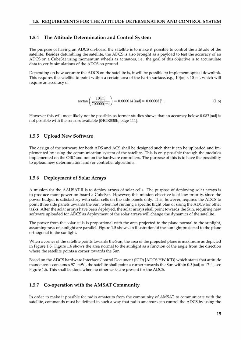
The purpose of having an ADCS on-board the satellite is to make it possible to control the attitude of thesatellite. Besides detumbling the satellite, the ADCS is also brought as a payload to test the accuracy of anADCS on a CubeSat using momentum wheels as actuators, i.e., the goal of this objective is to accumulatedata to verify simulations of the ADCS on ground.
Depending on how accurate the ADCS on the satellite is, it will be possible to implement optical downlink.This requires the satellite to point within a certain area of the Earth surface, e.g., 10 [m]× 10 [m], which willrequire an accuracy of
arctan(
10 [m]700000 [m]
)= 0.000014 [rad]≈ 0.00008 []. (1.6)
However this will most likely not be possible, as former studies shows that an accuracy below 0.087 [rad] isnot possible with the sensors available [04GR830b, page 111].
1.5.5 Upload New Software
The design of the software for both ADS and ACS shall be designed such that it can be uploaded and im-plemented by using the communication system of the satellite. This is only possible through the modulesimplemented on the OBC and not on the hardware controllers. The purpose of this is to have the possibilityto upload new determination and/or controller algorithms.
1.5.6 Deployment of Solar Arrays
A mission for the AAUSAT-II is to deploy arrays of solar cells. The purpose of deploying solar arrays isto produce more power on-board a CubeSat. However, this mission objective is of low priority, since thepower budget is satisfactory with solar cells on the side panels only. This, however, requires the ADCS topoint three side panels towards the Sun, when not running a specific flight plan or using the ADCS for othertasks. After the solar arrays have been deployed, the solar arrays shall point towards the Sun, requiring newsoftware uploaded for ADCS as deployment of the solar arrays will change the dynamics of the satellite.
The power from the solar cells is proportional with the area projected to the plane normal to the sunlight,assuming rays of sunlight are parallel. Figure 1.5 shows an illustration of the sunlight projected to the planeorthogonal to the sunlight.
When a corner of the satellite points towards the Sun, the area of the projected plane is maximum as depictedin Figure 1.5. Figure 1.6 shows the area normal to the sunlight as a function of the angle from the directionwhere the satellite points a corner towards the Sun.
Based on the ADCS hardware Interface Control Document (ICD) [ADCS HW ICD] which states that attitudemanoeuvres consumes 97 [mW], the satellite shall point a corner towards the Sun within 0.3 [rad]≈ 17 [], seeFigure 1.6. This shall be done when no other tasks are present for the ADCS.
1.5.7 Co-operation with the AMSAT Community
In order to make it possible for radio amateurs from the community of AMSAT to communicate with thesatellite, commands must be defined in such a way that radio amateurs can control the ADCS by using the
15

1.5. REQUIREMENTS FOR THE ATTITUDE DETERMINATION AND CONTROL SYSTEM
Sunlight
Satellite Projection of Sunlight
(a) Projection of 1 side.
Sunlight
Satellite
Projection of Sunlight
(b) Projection of 3 sides.
Figure 1.5: Illustration of the area of the satellite which is coveredby the sunlight projected to the plane orthogonal to the sunlight.
0 0.1 0.2 0.3 0.4 0.5 0.6 0.7 0.8 0.9 11.3
1.4
1.5
1.6
1.7
1.8
1.9
2.0
2.1
2.2
2.3
Angle [rad]
Pow
er [W
]
Figure 1.6: Area of the sunlight absorbed by the satellite, de-scribed by the angle between the diagonal of the Satellite BodyReference Frame and the sunlight, assuming rays of sunlight areparallel.
16

1.5. REQUIREMENTS FOR THE ATTITUDE DETERMINATION AND CONTROL SYSTEM
AX.25 protocol after the previous mission objectives have been fulfilled.
1.5.8 System Demands for ADCS
All the requirements shall be met with a confidence interval of 2σ equal to 95.44 [%].
1. The ADCS shall be able to detumble the satellite from 0.1 [rad/s] to 0.0021 [rad/s] or below around eachaxis within 3 orbits.
2. The ADCS shall be able to rotate the satellite at an angular velocity of at least 0.0045 [rad/s].
3. The ADCS shall be designed so it is possible to upload new determination and control algorithms.
4. The ADCS shall be able to maintain a given attitude for the satellite within 0.087 [rad] ≈ 5 [].
17

Modelling 2To be able to test the ADCS a simulation environment must be available. The models needed for this aredescribed in the following chapter.
To define vectors in space a reference frame is required, and to ease calculations a number of different co-ordinate systems are defined. After defining the coordinate systems, the environment will be modelled.This includes an ephemeris model, modelling of the disturbances affecting the satellite in LEO, an Earthalbedo model and an orbit propagator model, which is needed in the modelling of the disturbances and themodelling of the magnetic field model.
Furthermore, to determine how the environment is affecting the satellite, the dynamics and kinematics ofthe satellite are modelled.
In order to simulate the ACS the actuators on the satellite, which includes magnetorquers and momentumwheels, will be modelled.
The simulation environment is implemented in SIMULINK, and is presented in the end of this chapter.
2.1 Coordinate Systems
In this section the coordinate systems used for describing the attitude and the orbit of the satellite are intro-duced.
2.1.1 Orbital Elements
Before describing the coordinate systems used, the basic theory and the terms used in orbital mechanics arepresented. As source for this section [Wertz, Chapter 2 and 3] are used.
Kepler’s First Law: If two objects in space interact gravitationally, each will describe an orbit thatis a conic section with the center of mass at one focus. If the bodies are permanently associated,their orbits will be ellipses; if they are not permanently associated, their orbits will be hyperbo-las.
Kepler’s Second Law: If two objects in space interact gravitationally (whether or not they move inclosed elliptical orbits), a line joining them sweeps out equal areas in equal intervals of time.
Kepler’s Third Law: If two objects in space revolve around each other due to their mutual gravi-tational attraction, the sum of their masses multiplied by the square of their period of mutualrevolution is proportional to the cube of the mean distance between them. Hence
(m+M)P2 =4π2
Ga3, (2.1)
18

2.1. COORDINATE SYSTEMS
where P is their mutual period of revolution, a is the mean distance between them, m and M arethe two masses, and G is Newton’s gravitational constant.
Of the two revolving objects the one with the greatest mass is called the primary, and the less massive objectis called the secondary. If the mass of the satellite is denoted m, and the mass of the Earth is denoted M themass of the satellite is considered negligible,
m+M ≈M. (2.2)
Thus in the case of a satellite orbiting the Earth it follows from Kepler’s laws, that the trajectory of the satelliteis an ellipse with the center of the Earth at the one focus.
Figure 2.1: Satellite orbit.
An example of a satellite orbit is depicted in Figure 2.1 and an orthogonal view of the orbit is shown inFigure 2.2. In order to mathematically describe orbits the following terms are used.
Vernal equinox (g) is the line connecting the center of the Earth and the center of the Sun where the ecliptic,which is the plane of the Earths orbit around the Sun, crosses the equator, i.e., spring equinox. Dueto the precession and nutation of the Earth the direction of vernal equinox must be associated with aspecific year to give an unambiguous definition of the direction in space.
Line of nodes is the line through the two points of intersection between the satellite orbit and the referenceplane, typically the equatorial plane of the Earth. The point in the orbit where the satellite crosses fromsouth to north is called the ascending node.
19

2.1. COORDINATE SYSTEMS
Figure 2.2: Orthogonal view of an orbit.
Longitude of ascending node (Ω) is the angle from vernal equinox to the ascending node. Note that thisangle lies in the equatorial plane.
Perigee direction is the point in the orbit closest to the center of mass of the primary (the center of the Earth)this is often referred to as the barycenter.
Argument of perigee (ω) is the angle from the ascending node to the perigee direction.
Inclination (i) is the angle from the equatorial plane to the orbit plane.
The geometry of an ellipse is shown in Figure 2.3.
An ellipse is one of the four conic sections. Given two arbitrary points called foci an ellipse is describedgeometrically as the set of points for which the sum of the distances to the two foci is a given constant, 2a.The quantity 2a is also called the major axis of the ellipse, i.e., the width of the ellipse measured on a linethrough the two foci.
The eccentricity, e, describes the shape of an ellipse and is defined as the ratio
e =ca
=
√(a2−b2)
a, (2.3)
where c is half the distance between the two foci. For a circular orbit this ratio is, e = 0, meaning that the twofoci coincides, and for an elliptic orbit 0 < e < 1. The terms a, b and c are shown in Figure 2.3. For furtherinformation about ellipses see [Weisstein Ellipse].
2.1.2 Reference Frames
When dealing with ADCS for a satellite certain features as its orbit, the environment and attitude need tobe described. To describe the orientation of an object in space, a reference frame must be defined. As thesatellite can be observed from different points of view, a number of reference frames suitable for attitudedetermination and control purposes need to be defined. The reference frames used in this project is definedas a right-handed 3-dimensional cartesian coordinate system described by three mutually perpendicular unit
20

2.1. COORDINATE SYSTEMS
b
c
a
aSemimajor axis
Semiminor axis
focusfocus
Barycenter
Figure 2.3: The geometry of an ellipse.
vectors. When the reference frames are defined, it is possible to model the satellite and the environment ofthe satellite. Below is the list of the reference frames used in the AAUSAT-II project.
• Earth Centered Inertial reference frame - ECI
• Earth Centered Earth Fixed reference frame - ECEF
• Orbit Reference Frame - ORF
• Satellite Body Reference Frame - SBRF
• Controller Reference Frame - CRF
Earth Centered Inertial Reference Frame
An inertial reference frame is needed to have a non-accelerating point of view in which Newton’s laws ofmotion applies. As the AAUSAT-II will be launched into a Low Earth Orbit (LEO) the Earth will be theprimary object, and therefore an Earth Centered Inertial reference frame (ECI) system could be used as theinertial reference frame.
Unfortunately the ECI reference frame is not an ideal inertial reference frame as it is accelerating, due tothe fact that the Earth is orbiting the Sun. Thus a more precise inertial reference frame eliminating thisacceleration would be a Sun centered inertial reference frame. However, the Sun orbits the center of theMilky Way galaxy and so forth. So unless the inertial reference frame is defined with its origo in the centerof the Universe (hard to determine) it will never be ideal. However, choosing a non Earth centered referenceframe complicates the required calculations, and because the acceleration caused by the Earth orbiting theSun is considered negligible, the ECI reference frame is used in this project.
The ECI reference frame is illustrated in Figure 2.4. It is defined as a right handed cartesian coordinatesystem, having its origo in the center of the Earth. The x-axis is in the direction of vernal equinox g, the z-axis is perpendicular to the equatorial plane with the positive direction going through the geographic NorthPole of the Earth, and the y-axis is the cross product between the z-axis and the x-axis.
Earth Centered Earth Fixed Reference Frame
Some calculations can be simplified by using a reference frame that rotates with the Earth. This means thatpoints on the Earth surface such as ground stations are fixed in this frame. Also some environmental model-ling depends on the spacecraft position relative to a specific point on the Earth surface. For this purpose theEarth Centered Earth Fixed (ECEF) reference frame is introduced.
21

2.1. COORDINATE SYSTEMS
Geografic north pole
Equator
Direction of Vernal
Equinox
Z
X
Y
Rotational
axis
Figure 2.4: The Earth Centered Inertial reference frame.
The ECEF is illustrated in Figure 2.5. It is defined with origo in the center of the Earth. The z-axis is theEarth rotation axis and the positive direction is through the North Pole. The x-axis is in the direction of theintersection between the equatorial plane (0 latitude) and the Greenwich meridian (0 longitude). The y-axisis the cross product between the z- and x-axis, thus forming a right handed cartesian coordinate system.
Geografic north pole
Equator
Z
X
Y
Rotational
axis
ator
Zero longitude
Zero latitude
Figure 2.5: The Earth Centered Earth Fixed reference frame.
Orbit Reference Frame
The Orbit Reference Frame (ORF) is an accelerating, thus non-inertial reference frame, with origo in thecenter of mass of the satellite. For the AAUSAT-II satellite this point is in orbit around the Earth. The x-axisof the right perpendicular coordinate system is in the nadir direction (towards the center of the Earth). Thez-axis is perpendicular to the orbit plane with the positive direction in the direction of the angular velocityvector of the orbit. The y-axis is the cross product between the z-axis and the x-axis. Notice that for a circularorbit the y-axis is parallel to the translatory velocity of the spacecraft orbit as depicted in Figure 2.6.
22

2.1. COORDINATE SYSTEMS
Geografic north pole
Equator
Z
X
Y
Rotational
axis
Parallel to the
velocity vector
YX
(nadir)
Z
Normal vector
to the oribital plane
Orbit
Figure 2.6: The Orbit Reference Frame for a circular orbit.
Satellite Body Reference Frame
The Satellite Body Reference Frame (SBRF) is fixed with respect to the body of the satellite. It is used to deter-mine the orientation of the on-board instrumentation. If some of the on-board instruments are dependent onthe orientation of the satellite e.g. a camera, it is convenient to define the SBRF with one of the axes parallelto the field of view of this instrument.
As the payload of the AAUSAT-II has no requirements to the pointing direction, the SBRF is defined suchthat it is convenient for use with the attitude determination and control system. The SBRF has its centerin the corner of the satellite opposite of the vertical momentum wheel according to [MECH-WWW]. Theaxes forms a right-handed coordinate system with the axes perpendicular to the satellite sides. Thereby theon-board sensors and actuators direction is defined by the SBRF. The SBRF is depicted in Figure 2.7. In thefigure only the momentum wheels are shown.
X
Y
Z
Figure 2.7: The AAUSAT-II Satellite Body Reference Frame.
Controller Reference Frame
Figure 2.8 shows the Controller Reference Frame (CRF) which is convenient for calculations involving thesatellite dynamics as all products of inertia are eliminated.
The origo of the CRF is in the center of mass of the satellite and the axes are defined with respect to the
23

2.1. COORDINATE SYSTEMS
principal axes of the satellite. The x-axis is the major axis of inertia, the y-axis the minor axis of inertiaand the z-axis is the cross product between the x-axis and the y-axis, thus forming a right handed cartesiancoordinate system.
X
Y
Z
COM
Figure 2.8: The AAUSAT-II Controller Reference Frame with re-spect to the principal axes, with origo placed in the center of mass(COM).
Because the satellite is non-spherical and have a non-uniform mass distribution, the center of mass willobviously not coincide precise with the geometric center of the satellite. The mass distribution of the satellitemust be computed in order to determine the center of mass and the principal axes, which are required fordefining the CRF. The mechanical team affiliated with the AAUSAT-II project, MECH [MECH-Mail] hascalculated and measured the inertia matrix relative to the SBRF to be
SI =
Ixx Ixy Ixz
Iyx Iyy Iyz
Izx Izy Izz
=
1377 −40.427 3.199
−40.427 1623 −69.578
3.199 −69.578 1569
·10−6, (2.4)
where SI is given in [kg ·m2], and the center of mass in the SBRF to be
SP =
Pcom,x
Pcom,y
Pcom,z
=
56.11
49.829
50.788
·10−3, (2.5)
where SP is given in [m]. The principal axes can be found by calculating the eigenvalues of the inertia matrix.The major axis is the eigenvector corresponding to the largest eigenvalue. The intermediate axis is the eigen-vector corresponding to the intermediate eigenvalue, and the minor axis is the eigenvector corresponding tothe smallest eigenvalue [Wie, page 331-339]. The eigenvalues of SI on matrix form corresponding to CI are
SIλ = CI =
1.3702 0 0
0 1.5240 0
0 0 1.6748
·10−3. (2.6)
The matrix comprised of the eigenvectors can be used for rotating the SBRF into the CRF.
24
2.2. EPHEMERIS
2.1.3 Coordinate System Transformations
Rotations of coordinate systems can be described by quaternions. Quaternions provide a singularity-freerepresentation of kinematics and provide a convenient product rule for successive rotations. In Appendix Aquaternions are defined and the fundamental algebraic properties of quaternions are described.
2.2 Ephemeris
In the following section a model of the rotation of the Earth, i.e. a rotation of ECI to ECEF, will be derived.
As input to the gravitational disturbance model, the position of the Earth, the Sun, and the Moon is needed.The description of the orbit of the Sun around the Earth is further used to determine the vector from thesatellite to the Sun.
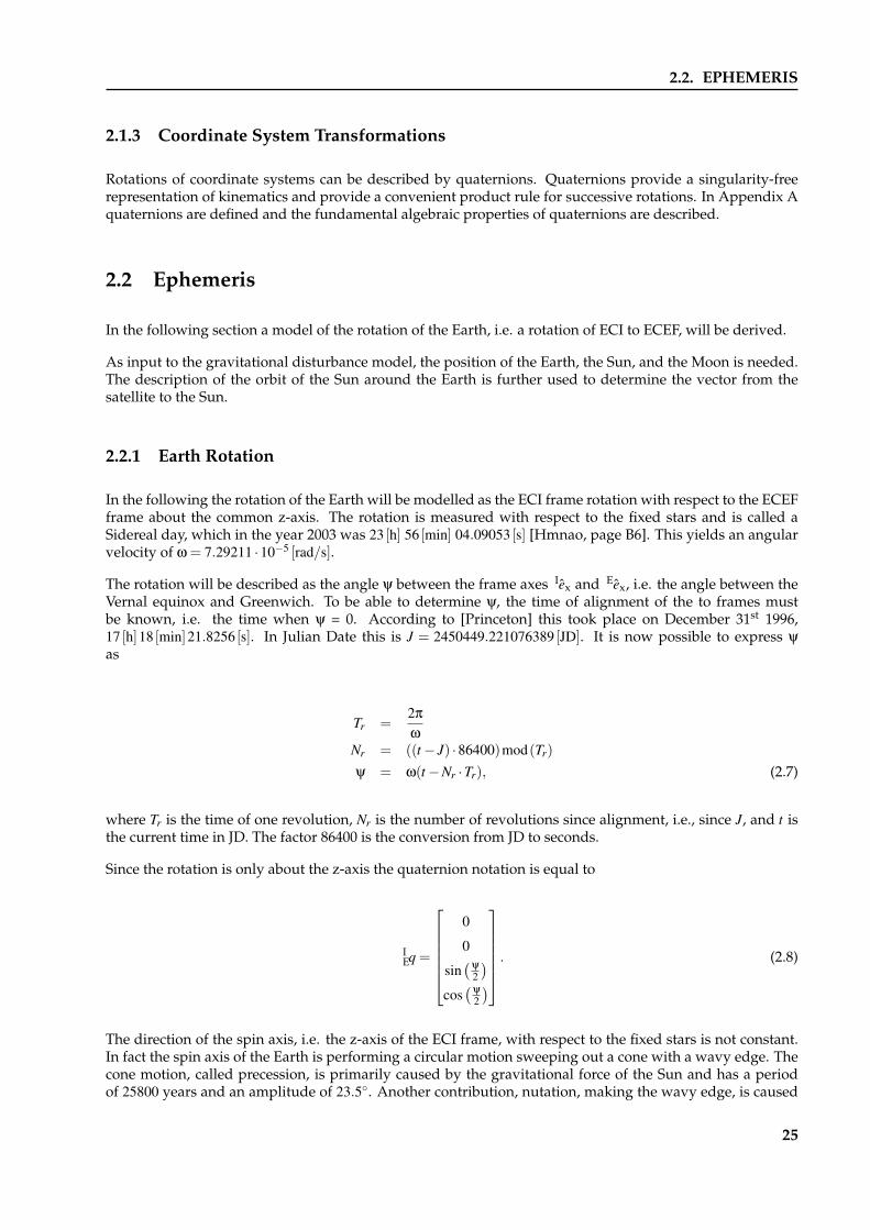
2.2.1 Earth Rotation
In the following the rotation of the Earth will be modelled as the ECI frame rotation with respect to the ECEFframe about the common z-axis. The rotation is measured with respect to the fixed stars and is called aSidereal day, which in the year 2003 was 23 [h] 56 [min] 04.09053 [s] [Hmnao, page B6]. This yields an angularvelocity of ω = 7.29211 ·10−5 [rad/s].
The rotation will be described as the angle ψ between the frame axes Iex and Eex, i.e. the angle between theVernal equinox and Greenwich. To be able to determine ψ, the time of alignment of the to frames mustbe known, i.e. the time when ψ = 0. According to [Princeton] this took place on December 31st 1996,17 [h]18 [min]21.8256 [s]. In Julian Date this is J = 2450449.221076389 [JD]. It is now possible to express ψ
as
Tr =2π
ω
Nr = ((t− J) ·86400)mod(Tr)ψ = ω(t−Nr ·Tr), (2.7)
where Tr is the time of one revolution, Nr is the number of revolutions since alignment, i.e., since J, and t isthe current time in JD. The factor 86400 is the conversion from JD to seconds.
Since the rotation is only about the z-axis the quaternion notation is equal to
IEq =
0
0
sin(
ψ
2
)cos
(ψ
2
)
. (2.8)
The direction of the spin axis, i.e. the z-axis of the ECI frame, with respect to the fixed stars is not constant.In fact the spin axis of the Earth is performing a circular motion sweeping out a cone with a wavy edge. Thecone motion, called precession, is primarily caused by the gravitational force of the Sun and has a periodof 25800 years and an amplitude of 23.5. Another contribution, nutation, making the wavy edge, is caused
25

2.2. EPHEMERIS
by the Moon. The period is 18,6 [years] and has an amplitude of 00′9′′21 [Sidi, page 22]. Nutation andprecession are not covered further since the effects of these are considered negligible.
2.2.2 Sun Position
The position of the Sun is described using keplerian orbit elements, as introduced in Section 2.1.1 and furtherin this section. The model places the Earth in the center with the Sun orbiting. Actually the Earth is orbitingthe Sun, but it makes no difference to the result. This section is based on [Wertz, page 140-145].
Since the eccentricity of the orbit of the Sun is small [Wertz, equation (5-46)] the following approach can beused. A starting point in time is needed where the exact position and velocity of the Sun is known. Themean anomaly MSE, of the Sun and the mean motion ns, of the Sun both on the 1st of January, 2000 at noonUTC, can be found in Table 2.1.
Parameter Value Unit
e 0.016751 [.]
MSE 357.528 []
ns 0.9856003 [/day]
c 23.4387 []
Table 2.1: Sun orbit elements obtained from [Princeton].
The mean anomaly Ms for a given time Ts, can be calculated as:
Ms = MSE +ns ·Ts, (2.9)
where Ts is the time measured in days since the 1st of January, 2000 at noon UTC. [Braeunig, Equation (1.29)]
The mean longitude of the Sun in the ecliptic plane can be described by LOS [Wertz, Equation (5-46) & (5-47)]
LOS = 279.696678+0.9856473354 ·Ms +1.918sin(Ms)+0.02sin(2Ms). (2.10)
Including the inclination of the ecliptic plane denoted c, leads to the following unit vector description of theSun orbiting the Earth in the ECI reference coordinate system
IRS =
cos(LOS)
cos(c)sin(LOS)
sin(c)sin(LOS)
(2.11)
The distance between the Sun and the Earth is described by [Wertz, Equation (5-48)]
Ds =1.495 ·108
(1− e2
)1+ ecos(Ms)
. (2.12)
26

2.2. EPHEMERIS
2.2.3 Sunlight Eclipse
Since the satellite is orbiting the Earth the line of sight from the satellite to the Sun will eventually be blockedby the Earth, i.e. the satellite is in eclipse, and as a consequence the sun sensor input will not be usable. Notonly the Earth but also the Moon will cause the satellite to be in eclipse. However, eclipses caused by themoon are relatively rare and have a short duration and are therefore not considered in the model.
Eclipse caused by the Earth happens when the distance from the center of the Earth perpendicular to theline of sight from the satellite to the Sun, IRE , is smaller than the radius of the Earth, rEarth. The problemis depicted in Figure 2.9. The incident light on the satellite due to light from the Sun being deflected in theatmosphere of the Earth in the short period after entering eclipse will be ignored.
Sun
Earth
Satellite
RSRSA
RS→SA
RE
R´SA
rEarth
Figure 2.9: Sunlight eclipse model. All the vectors are given inECI.
The vector IRE can be expressed asIRE = IRSA + IR
′SA. (2.13)
Furthermore IR′SA can be described as
IR′SA =
− IRSA · IRSA→S
‖ IRSA→S‖2IRSA→S (2.14)
where IRSA→S = IRS− IRSA is the vector from the satellite to the Sun.
Inserting (2.14) into (2.13) result in a term for ‖ IRE‖, which for ‖ IRE‖ < rEarth entails that the satellite is ineclipse, yields
‖ IRE‖=∣∣∣∣∣∣∣∣IRSA−
IRSA · IRSA→S
‖ IRSA→S‖2IRSA→S
∣∣∣∣∣∣∣∣ . (2.15)
2.2.4 Moon Position
The orbit of the Moon is rather complex and will not be described, since ephemeris modelling is not the maintopic in this project.
27

2.3. DISTURBANCE MODELLING
In the SIMULINK implementation position of the Moon will be handled by a toolbox from Princeton SatelliteSystem. A few corrections has been made by the previous groups (see [04GR830b] and [04GR830a]) to allowcontinuous position updates.
2.3 Disturbance Modelling
This section describes the main disturbances affecting the attitude of the satellite. Four disturbances areconsidered for the model, these are
• Aerodynamic drag
• Gravity gradient
• Magnetic residual
• Solar radiation
This implies that the total disturbance torque on the satellite can be calculated in the SBRF as
SNext = SNdrag + SNGG + SNmag + SNR. (2.16)
Where SNdrag is the torque caused by the aerodynamic drag, SNGG is the torque caused by the gravitygradient, SNmag is the torque caused by the interaction between the Earth’s magnetic field and the satellitesmagnetic residual dipole and SNR is the torque caused by the solar radiation.
2.3.1 Aerodynamic Drag Disturbance
For a satellite in LEO the main disturbance torque is excerted by aerodynamic drag [Wertz, page 573]. Thedrag arises from the friction between the satellite and the atmosphere and is in the opposite direction ofthe satellites velocity vector. The force d f drag acting on an infinitesimal surface element dA with the normalvector N, is given by
d f drag =−12
ρCD‖V‖2(N ·V )V dA, (2.17)
where V is a unit vector in the direction of the satellites translational velocity, ρ is the atmospheric densityand CD is the drag coefficient. Since there is no measured value available for CD, it can be set to 2, accordingto [Wertz, page 573-574]. By integrating (2.17) over the exposed area, the total aerodynamic drag can becalculated. For objects with a simple and symmetric structure this can be simplified to
f drag =−12
ρCDA‖V‖2V , (2.18)
where A is the total exposed area of the satellite, measured in a plane perpendicular to the motion [Serway &Beichner, page 165-166]. This means that the aerodynamic torque SNdrag acting on the satellite due to f dragcan be written as
SNdrag = SCP× S f drag, (2.19)
28

2.3. DISTURBANCE MODELLING
where SCP is a vector from the center of mass to the center of pressure on the satellite. The center of pressureis the geometrical center of the exposed cross sectional area1.
2.3.2 Gravitational Disturbances
The gravitational disturbance model must contain the following forces
• Gravitational forces from the Sun and the Moon
• The Earth’s zonal harmonics
• The gravity gradient
The gravitational forces from the Sun and the Moon, will influence the orbit of the satellite and shouldtherefore be included in the disturbance model.
The Earth’s zonal harmonics arise from the fact that the Earth is not a perfect sphere, i.e., the radius is largerat the equator than at the poles, which entail that the Earth’s gravity field varies. This will affect the orbit ofthe satellite and should therefore be included in the disturbance model.
As the satellite is non-spherical and has a non-uniform mass distribution, it will experience a gravitationaltorque around the center of mass, due to Earth’s gravitational force.
Sun and Moon Gravity Disturbance
For calculating the gravitational disturbance from the Sun and the Moon, Newton’s law of universal grav-itation [Serway & Beichner, page 424-425] is used. A vector from the satellite to the Sun is calculated asIRSA→S = IRS − IRSA, as seen in Figure 2.9. The vector IRS is from the center of the Earth to the Sun in theECI and IRSA is a vector from the center of the Earth to the satellite in the ECI. IRSA→S is used to calculate theforce the Sun excerts on the satellite
IFGS = GmSmSA
‖ IRSA→S‖2 ·IRSA→S
‖ IRSA→S‖= G
mSmSA
‖ IRSA→S‖3IRSA→S, (2.20)
where G is the gravitational constant, ms is the mass of the Sun and mSA is the mass of the satellite. Theequation for the force between the satellite and the Moon are of the same structure.
IFGM = GmMmSA
‖ IRSA→M‖3IRSA→M, (2.21)
where mM is the mass of the Moon and IRSA→M is a vector from the satellite to the Moon.
Earth Zonal Harmonics
Because the Earth have a non-uniform mass distribution the gravitational field vary, depending on the po-sition of the satellite. This is known as the Earth’s zonal harmonics. This section is based on [Serway &
1In the same way that the weight of all the satellite components act through a single point, the center of mass, theaerodynamic forces act through a single point called the center of pressure.
29

2.3. DISTURBANCE MODELLING
Beichner, page 435-437] and [Wertz, page 123-126]. If a particle is placed in the Earth’s gravitational field, itwill experience a force
F =−GME m‖r‖2 · r, (2.22)
where ME is the mass of the Earth, G is the gravitational constant, r is a vector from the center of the Earthto the particle. The minus indicates that the field points toward the center of the Earth. Now the Earthgravitational potential, U can be defined as
U =−GME
‖r‖. (2.23)
From (2.23), (2.22) can be expressed as the gradient of a scalar potential
F =−GMEm‖r‖2 r =−m∇U, (2.24)
where U can be expressed as
U ∼=GME
‖r‖[U0 +UJ2 +UJ3 +UJ4 ], (2.25)
where
U0 = −1, (2.26)
UJ2 =( rEarth
‖RSA‖
)2J2
12(3cos2
θ−1), (2.27)
UJ3 =( rEarth
‖RSA‖
)3J3
52(cos3
θ− 35
cosθ), (2.28)
UJ4 =( rEarth
‖RSA‖
)4J4
358
(cos4θ− 6
7cos2
θ+335
). (2.29)
The radius of the Earth is denoted rEarth and J2, J3 and J4 are the zonal harmonic coefficients. Now thegradient of U can be found as
∇U =
∂U
∂‖RSA‖1
‖RSA‖∂U∂φ
1‖RSA‖sinφ
∂U∂θ
, (2.30)
which yields
∇U =
−GME
(− 1‖RSA‖2 + 3
2rE J2(3c2θ−1)
‖RSA‖4 +10 r3E J3(c3θ− 3
5 cθ)‖RSA‖5 + 175
8r4
E J4(c4θ− 67 c2θ+ 3
35 )‖RSA‖6
)0
GME‖RSA‖2sφ
(−3 r2
E J2cθsθ
‖RSA‖2 + 52
r3E J3(−3c2θsθ+ 3
5 sθ)‖RSA‖3 + 35
8r4
E J4(−4c3θsθ+ 127 cθsθ)
‖RSA‖4
) , (2.31)
30

2.3. DISTURBANCE MODELLING
where c ≡ cos and s ≡ sin and rE is the radius of the Earth. Now, the force excerted by the zonal harmonicscan be found according to (2.24).
Gravity Gradient
The gravity between a satellite of mass, mSA, and the Earth with mass, ME , at a distance, ‖RSA‖, from theEarth’s center, has a magnitude of
‖F‖= GMEmSA
‖RSA‖2 , (2.32)
where G is the gravitational constant. If m1 and m2, in Figure 2.10, are two equal mass elements of thesatellite, they will not experience the same gravity. This is due to the fact, that the gravity depends on theinverse square of the distance between the mass elements and the Earth’s center. In the scenario depicted inFigure 2.10 F1 will be greater than F2 and the satellite will experience a counter-clockwise torque around thecenter of mass.
F2
Direction of Nadir vector
F1
m
m
1
2
Center of mass
Figure 2.10: Illustration of the gravity gradient torque.
The equation for the torque can be expressed as [Wertz, page 567]
SNGG =3µ
‖ SRSA‖3
[SRSA× ( SI · SRSA)
], (2.33)
where µ is the gravitational constant multiplied with the mass of the Earth, SRSA is a vector from the centerof the Earth to the satellite and SI is the moment of inertia tensor2.
2.3.3 Magnetic Residual Disturbance
The magnetic field of the Earth interacts with the residual magnetic dipole of the satellite, which causes atorque around the center of mass of the satellite. The residual magnetic dipole of the satellite is caused bythe current running through the wires and PCBs on the satellite. The magnetic disturbance can, accordingto [Wertz, page 575], be expressed as
SNmag = Sm× SB, (2.34)
2I is called a tensor because it has specific transformation properties under a real orthogonal transformation.
31

2.3. DISTURBANCE MODELLING
where Sm is the residual magnetic dipole of the satellite and SB is the magnetic field of the Earth. The residualmagnetic dipole of the satellite should be modelled, since it cannot be assumed to be constant, because itdepends on the amount of current running through the wiring on the satellite. However, at the time ofthis writing the PCBs of the satellite are subjected to changes, whereby the residual magnetic dipole of thesatellite will not be modelled.
2.3.4 Radiation Disturbance
Radiation hitting the surface of the satellite will cause a torque around the center of mass. There are severalradiation sources for this torque, but the major ones are direct solar radiation, solar radiation reflected bythe Earth and its atmosphere, i.e. the Earth’s albedo and radiation emitted from the Earth. The radiationemitted from the Earth will not be considered since it is small compared to the others [Wertz, page 571]. Themagnitude of the solar radiation force, FR, is given by
‖FR‖= KAP, (2.35)
where P is the momentum flux from the Sun, given by P = 4.4 ·10−6 [kg/ms2], K is a dimensionless constantin the range 0 ≤ K ≤ 2, depending on the amount of the sunlight the satellite surface reflects and A is thecross-sectional area perpendicular to the vector from the satellite to the Sun exposed to the Sun [Wertz, page64-65].
The force will act in the opposite direction of the vector from the satellite to the Sun, IRSA→S = IRS − IRSAshown in Figure 2.9. Therefore a negative unit vector in the direction of IRSA→S is multiplied with the force.
IFR =−KAP IRSA→S. (2.36)
A rotation of IFR to SBRF can be made, and the disturbance torque in SBRF can be expressed as
SNR = SFR× SRcom, (2.37)
where SRcom is a vector from the center of mass of the satellite, to the geometrical center. This equationconsiders only the radiation coming directly from the Sun and not from the albedo of the Earth.
2.3.5 Total Disturbance Torque
The disturbances have been analyzed and modelled and an equation expressing the total disturbance torquecan now be derived as
SNext = SNdrag + SNGG + SNR ⇔ (2.38)
SNext = SCP× S f drag +3µ
‖ SRSA‖3
(SRSA× ( SI · SRSA)
)+ SFR× SRcom. (2.39)
The torque generated by magnetic residuals has been omitted since no model of the residual magnetic dipoleof the satellite is available.
32

2.4. EARTH ALBEDO
2.4 Earth Albedo
The reflectivity of the surface of the Earth causes a percentage of the incident sunlight to be reflected backinto space where the satellite is orbiting. This phenomenon is called the Earth albedo effect. The Earth’sreflectivity is on average 30 [%] [Wertz & Larson, page 428], but varies depending on the position on thesurface of the Earth. E.g., at the poles the reflectivity can be as high as 95 [%] and at the equator as low as10 [%].
NASA is in co-operation with Goddard Space Flight Center mapping the reflectivity in the Total OzoneMapping Spectrometer (TOMS) experiment [NASA/GSFC], and measurements from the TOMS experimentare shown in Figure 2.11.
Figure 2.11: Reflectivity of the Earth. Bright is high reflectivityand dark is low reflectivity (generated using SIMULINK albedotoolbox).
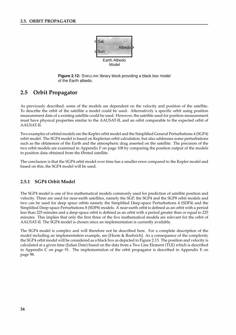
Using data from the TOMS experiment [Bhanderi] has developed an albedo toolbox including the albedoSIMULINK library model shown in Figure 2.12. This library block will be used in the simulations as a blackbox model with sun and satellite vectors in the ECEF as input and a matrix describing the albedo in [W/m2]within the entire field of view of the satellite is provided as the output. In the albedo toolbox there is also aMATLAB function taking the zenith vector, a normal vector to a sun sensor plane and the albedo matrix fromthe albedo library block as input and providing the total albedo contribution to the sun sensor in the givenplane as output. However, this function has been modified to accommodate two normal vector input as thisis enough to describe all normal vectors to the sun sensor planes for the cubic AAUSAT-II. The modifiedfunction then returns the albedo received on each sun sensor as a vector.
33
2.5. ORBIT PROPAGATOR
Albedo
Sat
Sun
Earth AlbedoModel
Figure 2.12: SIMULINK library block providing a black box modelof the Earth albedo.
2.5 Orbit Propagator
As previously described, some of the models are dependent on the velocity and position of the satellite.To describe the orbit of the satellite a model could be used. Alternatively a specific orbit using positionmeasurement data of a existing satellite could be used. However, the satellite used for position measurementmust have physical properties similar to the AAUSAT-II, and an orbit comparable to the expected orbit ofAAUSAT-II.
Two examples of orbital models are the Kepler orbit model and the Simplified General Perturbations 4 (SGP4)orbit model. The SGP4 model is based on Keplerian orbit calculation, but also addresses some perturbationssuch as the oblateness of the Earth and the atmospheric drag asserted on the satellite. The precision of thetwo orbit models are examined in Appendix F on page 108 by comparing the position output of the modelsto position data obtained from the Ørsted satellite.
The conclusion is that the SGP4 orbit model over time has a smaller error compared to the Kepler model andbased on this, the SGP4 model will be used.
2.5.1 SGP4 Orbit Model
The SGP4 model is one of five mathematical models commonly used for prediction of satellite position andvelocity. Three are used for near-earth satellites, namely the SGP, the SGP4 and the SGP8 orbit models andtwo can be used for deep space orbits namely the Simplified Deep-space Perturbations 4 (SDP4) and theSimplified Deep-space Perturbations 8 (SDP8) models. A near-earth orbit is defined as an orbit with a periodless than 225 minutes and a deep-space orbit is defined as an orbit with a period greater than or equal to 225minutes. This implies that only the first three of the five mathematical models are relevant for the orbit ofAAUSAT-II. The SGP4 model is chosen since an implementation is currently available.
The SGP4 model is complex and will therefore not be described here. For a complete description of themodel including an implementation example, see [Hoots & Roehrich]. As a consequence of the complexitythe SGP4 orbit model will be considered as a black box as depicted in Figure 2.13. The position and velocity iscalculated at a given time (Julian Date) based on the data from a Two Line Element (TLE) which is describedin Appendix C on page 91. The implementation of the orbit propagator is described in Appendix E onpage 98.
34

2.6. MAGNETIC FIELD MODEL
SGP4
TLE
Julian date
Position vector
Velocity vector
Figure 2.13: The SGP4 orbit model is considered a black box.
2.6 Magnetic Field Model
To be able to emulate the output of the magnetometer of the satellite a model describing the magnetic fieldof the Earth is needed. In the following, a short introduction to the magnetic field of the Earth is given andthe chosen model is described.
The magnetic field observable on the surface of the Earth can be categorized in internal sources and externalsources. The primary internal contribution to the magnetic field is generated in the fluid outer core by a self-exciting dynamo process. Electrical currents flowing in the slowly moving molten iron generate the magneticfield. The other internal source is the magnetic field generated by magnetic materials in the crust of the Earth.The external sources are due to magnetic fields induced by currents in the Ionosphere and Magnetosphere.The external sources can be omitted since the magnitude of the magnetic field due to external sources arelow compared to the magnetic field of the Earth and furthermore the orbit of the AAUSAT-II is expected tobe in a higher altitude than the upper bounds of the Ionosphere [BGS].
2.6.1 International Geomagnetic Reference Field model
The International Geomagnetic Reference Field (IGRF) model is used to describe the magnetic field of theEarth. It is an empirical representation of the main field without any external sources. The IGRF model uses aset of coefficients which has been modelled using data from geomagnetic measurements from observatories,ships, aircrafts and satellites, e.g., the Danish Ørsted satellite. Omitting external sources, the main magneticfield B, is the negative gradient of a scalar potential V , B(r,θ,φ, t) =−∇V (r,θ,φ, t), which according to [IAGAV-MOD] can be represented by a truncated series expansion as
V (rEarth,θ,φ, t) = Rn
∑n=1
(R
rEarth
)n+1 n
∑m=0
(gmn (t)cos(mφ)+hm
n (t)sin(mφ))Pmn (θ) (2.40)
where,
rEarth Distance from the center of the Earth
θ Colatitude, i.e. 90 []- latitude
φ Longitude
R Reference radius (6371.2 [km])
gmn (t), hm
n (t) coefficients at time t
Pmn (θ) Schmidt semi-normalized associated Legendre functions of degree n and order m.
The main-field coefficients change with time as the core-generated field changes. This variation is assumedto be constant over intervals of five years.
35

2.7. SATELLITE DYNAMICS AND KINEMATICS
2.7 Satellite Dynamics and Kinematics
This section contains the derivation of the dynamic and kinematic equations of the satellite. The dynamicdifferential equation of the satellite describes how torques acting on the satellite influence the rotationalacceleration of the satellite. The kinematic differential equation of the satellite describes the time dependentrelationship between different reference frames. The following section is based on [Wertz, page 516-523].For the section concerning kinematics [Wie, page 307-328] is used. Whenever an equation is copied from asource a citation will be given. Appendix A provides a description of the fundamental algebraic propertiesof quaternions which are extensively used for these equations.
2.7.1 Dynamic Equation of the Satellite
This subsection contains the dynamic differential equation of the satellite, which is based on Newton’s lawsof motion and Euler’s laws of angular momentum.
When modelling a system it is basically a good idea to choose a simple model structure that gives an ade-quate description of the system. In order to derive the dynamic equation for the satellite a rigid body modelstructure is chosen.
Euler’s second equation given in inertial coordinates can be expressed as
d ILdt
= INext , (2.41)
where L is the angular momentum and Next are the external torques acting on the satellite. These exter-nal torques are disturbance torques which include aerodynamic drag, solar radiation, gravity gradient andmagnetic residual cf. Section 2.3. The internal torques are cancelled due to Newton’s third law.
The angular momentum of the satellite is defined as
LSA = Iω, (2.42)
where I is the moment of inertia tensor.
In order to express IL in the CRF the following equation is used
CL = CI C IL, (2.43)
where CI C is an attitude matrix from ECI to CRF. Taking the derivative yields
CL = CI C IL+ C
I CILCL = C
I C IL+C L. (2.44)
Comparing (2.44) with the translation theorem given in (2.45)
d CLdt
=d ILdt
−ω× IL, (2.45)
yields the following expression for the change in angular momentum given in the CRF
36

2.7. SATELLITE DYNAMICS AND KINEMATICS
CL =C Next−ω× CL, (2.46)
Besides the disturbance torques the satellite is also influenced by control torques from the magnetorquersand momentum wheels. The control torques from the momentum wheels will be modelled in the dynamicdifferential equation of the satellite. Control torques from the magnetorquers will be modelled separately,however the contribution from the magnetorquers will be included in the dynamic differential equation.
Due to the fact that the satellite contains momentum wheels, it cannot be considered a rigid body. However,it is still possible to derive the dynamic equation of the satellite using the equations for a rigid body model.With the angular momentum from the momentum wheels included the total angular momentum of thesatellite becomes
L = LSA +Lmw, (2.47)
where Lmw is the angular momentum of the momentum wheels. Inserting (3.39) in (2.47) yields
L = Iω+Lmw
Iω = L−Lmw
ω = I−1(L−Lmw). (2.48)
Substituting (2.48) into (2.46) yields the following equation for the total angular momentum of the satellite
CL =C Next− (I−1( CL−CLmw))× CL. (2.49)
It is important that the dynamic equation of the satellite is calculated in the CRF, otherwise the moment ofinertia will be a time varying tensor. By choosing the CRF as consisting of the principle axes the product ofinertia becomes 0, thereby yielding the moment of inertia tensor matrix [Wertz, page 519]
CI =
I1 0 0
0 I2 0
0 0 I3
. (2.50)
Since the CRF will be used in the expression of the dynamic equation the superscript denoting the referenceframe, will not be used in the further derivation of the dynamic equation.
Inserting (2.50) in (2.49) and calculating the cross product yieldsL1
L2
L3
=
Next,1− (L2−Lmw,2)L3I−1
2 +(L3−Lmw,3)L2I−13
Next,2− (L3−Lmw,3)L1I−13 +(L1−Lmw,1)L3I−1
1
Next,3− (L1−Lmw,1)L2I−11 +(L2−Lmw,2)L1I−1
2
. (2.51)
Instead of expressing the dynamic differential equations in terms of the time derivative of the total angularmomentum as in (2.51) it is simpler to express it in terms of the time derivative of the angular velocity. Thisis done by expressing (2.49) as
37

2.7. SATELLITE DYNAMICS AND KINEMATICS
Iω+ Lmw = Next− (I−1(L−Lmw))×L
Iω = Next− Lmw−ω× (Iω+Lmw). (2.52)
Then by introducing the skew symmetric matrix shown in (2.53) it is possible to substitute the cross productin (2.52) with a multiplication [Hughes, page 524-525]
S(ω) = ωT ×ω =−ω×ω
T =−
ω1
ω2
ω3
×[ω1 ω2 ω3
]
= −
ω1× ω1 ω1× ω2 ω1× ω3
ω2× ω1 ω2× ω2 ω2× ω3
ω3× ω1 ω3× ω2 ω3× ω3
=
0 −ω3 ω2
ω3 0 −ω1
−ω2 ω1 0
, (2.53)
(2.52) can now be expressed as
ω = I−1[Next +Nctrl−S(ω)(Iω+Lmw)], (2.54)
where the control torque, Nctrl is defined as
Nctrl = Nmt−Nmw. (2.55)
Nmt is the torque contributed by the magnetorquers and the Nmw is the torque applied to the momentumwheels which is defined as
Nmw = Lmw. (2.56)
The equation derived in (2.54) will be used in the system equations for the satellite.
2.7.2 Kinematic Equation for the Satellite
There are different methods to represent the kinematic differential equation of the satellite. These are thedirect cosine matrix (DCM) denoted the attitude matrix, Euler angles and quaternions. However, the attitudematrix representation suffers from redundance and the Euler angles suffer from singularities, which is whythis section contains the kinematic differential equation represented in terms of quaternions which only hasone redundant parameter.
38

2.7. SATELLITE DYNAMICS AND KINEMATICS
In order to derive the kinematic differential equation in terms of quaternions the attitude matrix given byEuler’s eigenaxis rotation theorem is used. This attitude matrix is derived in Appendix B and is expressedas
C =
cθ+ e2
1(1− cθ) e1e2(1− cθ)+ e3sθ e1e3(1− cθ)− e2sθ
e2e1(1− cθ)− e3sθ cθ+ e22(1− cθ) e2e3(1− cθ)+ e1sθ
e3e1(1− cθ)+ e2sθ e3e2(1− cθ)− e1sθ cθ+ e23(1− cθ)
, (2.57)
where cθ≡ cos(θ), sθ≡ sin(θ) and ei are the direction cosines of the Euler axis, which is bounded by e21 +e2
2 +e2
3 = 1
Based on Appendix A the following definitions for the quaternions are used in deriving the kinematic diffe-rential equation.
q1:3 = e1:3 sin(θ/2). (2.58)
q4 = cos(θ/2) (2.59)
q = (q1:3,q4) (2.60)
q21 +q2
2 +q23 +q2
4 = 1. (2.61)
It is now possible to express the attitude matrix given in (2.57) in terms of quaternions [Wie, page 318]yielding
C(q1:3,q4) =
1−2(q2
2 +q23) 2(q1q2 +q3q4) 2(q1q3−q2q4)
2(q2q1−q3q4) 1−2(q21 +q2
3) 2(q2q3−q1q4)
2(q3q1 +q2q4) 2(q3q2−q1q4) 1−2(q21 +q2
2)
. (2.62)
The kinematic differential equation for the attitude matrix method which is derived in Appendix B yields
C+S(ω)C = 0, (2.63)
where C is the attitude matrix from one reference frame to another, C is the time derivative of the sameattitude matrix and S(ω) is a 3×3 skew symmetric matrix containing the angular velocity.
From (2.63) the following vector composition for the angular velocity is given.
ω1 = C21C31 +C22C32 +C23C33 (2.64)ω2 = C31C11 +C32C12 +C33C13 (2.65)ω3 = C11C21 +C12C22 +C13C23. (2.66)
39

2.7. SATELLITE DYNAMICS AND KINEMATICS
In order to express (2.64), (2.65) and (2.66) in terms of quaternions (2.62) is used. This yields the followingequations
ω1 = 2(q1q4 + q2q3− q3q2− q4q1) (2.67)ω2 = 2(q2q4 + q3q1− q1q3− q4q2) (2.68)ω3 = 2(q3q4 + q1q2− q2q1− q4q3). (2.69)
One more equation is needed in order to obtain 4 equations with 4 unknowns. By differentiating (2.61) thelast equation is obtained
0 = 2(q1q1 + q2q2 + q3q3 + q4q4). (2.70)
The four equations (2.67), (2.68), (2.69) and (2.70) can be combined into matrix form which yields
ω1
ω2
ω3
0
= 2
q4 q3 −q2 −q1
−q3 q4 q1 −q2
q2 −q1 q4 −q3
q1 q2 q3 q4
q1
q2
q3
q4
. (2.71)
Since the 4×4 matrix in (2.71) is orthonormal the kinematic differential equation for the satellite in terms ofquaternions is given in the matrix form [Wie, page 327]
q1
q2
q3
q4
=12
0 ω3 −ω2 ω1
−ω3 0 ω1 ω2
ω2 −ω1 0 ω3
−ω1 −ω2 −ω3 0
q1
q2
q3
q4
. (2.72)
By defining a vector ω =[
ω1 ω2 ω3
]Tit is possible to express (2.72) in the compact form shown in (2.73)
q =12
q4ω−ω×q1:3
−ωT q1:3
=12
−S(ω) ω
−ωT 0
q =12
Ωq, (2.73)
where Ω is defined as
Ω =
0 ω3 −ω2 ω1
−ω3 0 ω1 ω2
ω2 −ω1 0 ω3
−ω1 −ω2 −ω3 0
There are certain advantages in using quaternions as a representation of rigid body rotation. As alreadymentioned the quaternions eliminate the redundancy and singularities that appear when expressing rigidbody rotation with the attitude matrix or Euler angles. Furthermore, the quaternion representation only
40

2.7. SATELLITE DYNAMICS AND KINEMATICS
consists of products and sums and it does not contain any trigonometric functions like the attitude matrixand Euler angles. This makes the rigid body rotation expressed in quaternions more suited for softwareimplementation as it is less computational demanding.
2.7.3 System Equations
Based on the derived dynamic and kinematic differential equations for the satellite, it is possible to expressthe system equations as
ω
q
︸ ︷︷ ︸
x
=
I−1(Next +Nctrl−S(ω)(Iω+Lmw))12 Ωq
︸ ︷︷ ︸
f (x,u,w)
(2.74)
ω
q
︸ ︷︷ ︸
y
=
13×3 03×4
04×3 14×4
︸ ︷︷ ︸
C
ω
q
︸ ︷︷ ︸
x
(2.75)
The system equations are constructed, based on the desire of an output containing the angular velocity, ω,and the attitude in terms of a quaternion, q. In order to keep the output matrix C simple, the angular velocityand the attitude quaternion are suitable choices for the state vector, x. In (2.74) the states are given by afunction, containing the state variables, the control signals and the disturbances denoted f (x,u,w). In (2.75)the notation 13×3 means a 3×3 identity matrix, i.e. the output matrix C becomes a 7×7 identity matrix.
Because the function f (x,u,w) is nonlinear it needs to be linearized, before it is possible to obtain the systemequations in state space form. The linearization of (2.74) can be found in Appendix D and it yields thefollowing linearized expression
˙q1:3
˙ω˙Lmw
︸ ︷︷ ︸
˙x
=
−S(ω) 1
2 13×3 03×3
03×3 I−1 [S(Iω)−S(ω)I+S(Lmw)] −I−1S(ω)
03×3 03×3 03×3
︸ ︷︷ ︸
A
q1:3
ω
Lmw
︸ ︷︷ ︸
x
+
03×3 03×3
I−1 −I−1
03×3 13×3
︸ ︷︷ ︸
B
Nmt
Nmw
︸ ︷︷ ︸
u
. (2.76)
Furthermore, the output equation is rewritten to include the same state vector as in (2.76). This yields thefollowing expression
y = y+ y, (2.77)
where
41

2.8. TRANSDUCERS
y =
13×3 03×3 03×3
03×3 13×3 03×3
03×3 03×3 13×3
︸ ︷︷ ︸
C
q1:3
ω
Lmw
︸ ︷︷ ︸
x
and y =
13×3 03×3 03×3
03×3 13×3 03×3
03×3 03×3 13×3
︸ ︷︷ ︸
C
q1:3
ω
Lmw
︸ ︷︷ ︸
x
The linear system equations in (2.76) and (2.77) can be used for both the control of the satellite in the form ofa state space model and for the determination of the attitude.
2.8 Transducers
The design of ACDS includes a full model of the system to be able to simulate the behaviour of the attitudeof the satellite in space. Therefore the sensors and the actuators need to be included in the model too.
On the AAUSAT-II three different types of sensors will be used.
Gyro A gyro measures the angular velocity of the satellite or the angle of rotation from an initial referencepoint, without any use of external references.
Magnetometer A magnetometer measures the direction and size of the magnetic field of the Earth which iswhy it can only be used in the vicinity of Earth (LEO).
Photo diode A photo diode is used to measure the current induced from the exposure of the diode to sun-light. This current induced is dependent of the angle of attack of the sunlight.
The actuators used on the AAUSAT-II will be
Magnetorquers The magnetorquers consist of 3 coils, one placed perpendicular to each axis on the satelliterelative to the SBRF. The magnetorquers are able to create a magnetic field which can create a torque onthe satellite when the magnetic field is perpendicular to the magnetic field of the Earth. When using themagnetorquers, the magnetometers must be turned off to avoid contamination of the magnetometerreadings.
Momentum Wheels The momentum wheels consist of 3 motors on which a load is mounted. The momen-tum wheels are placed one on each axis of the satellite. Spinning a momentum wheel up and downloads and unloads angular momentum from the satellite into the momentum wheels and makes thesatellite change attitude.
The modelling of the sensors has been made and implemented in the SIMULINK model by the ADS group,05gr833 [ADS05], and this will not be further described in this report. The following section describes themodelling of the actuators used on AAUSAT-II.
2.9 Actuator Modelling
In this section the models for the attitude control actuators on-board the spacecraft will be described. Themomentum wheels are used for quick and small changes in attitude and the magnetorquers are used todesaturate the momentum wheels or for slow changes in attitude.
42

2.9. ACTUATOR MODELLING
2.9.1 Magnetorquer Model
The magnetorquers used on AAUSAT-II are rectangular coils with the sides Sx1,Sx2,Sy1,Sy2, as shown inFigure 2.14. The arrows indicate the direction of the current in the coil.
B field vector
Sx1
Sy1
X
Y
Z
Sy2
Sx2
Figure 2.14: Diagram of a magnetorquer.
When placed in a magnetic field the force F acting on each side of the coil can be described by (2.78)
F = n · I ·S×B (2.78)
where n is the number of windings of the coil, I is the current in the coil and B is the magnetic field vector.The resulting force Fres is then
Fres =2
∑i=1
n · I ·Sxi×B+2
∑i=1
n · I ·Syi×B (2.79)
Figure 2.15 shows the magnetorquer in a magnetic field and the forces acting on each side of the coil.
Sx1
xB
B field vector
Sx1
Sy1
xB
Y
X
Sy1
Z
Sy2
Sy2
xB
Sx2
Sx2
xB
Figure 2.15: Diagram of a magnetorquer, the B-field and theresulting forces.
Because the current runs in a loop the resulting force Fres will be equal to zero. This means that the orbit ofthe satellite cannot be changed by the magnetorquer. It can, however, create a torque because the forces areacting on the sides of the coil, and this torque can be used to adjust the attitude of the satellite.
The magnitude of the torque can be found by projecting the force vectors found in (2.78) onto the plane witha normal vector that lies in the coil plane and is perpendicular to the coil element vector on which the force
43

2.9. ACTUATOR MODELLING
acts. One such normal vector is the coil vectors orthogonal to the coil vector on which the force acts. Theprojection matrix is calculated from a normal vector with unit length:
Nxu =Sx2
|Sx2|(2.80)
The projection matrix:
Qx = I−Nxu ·NxuT (2.81)
Figure 2.16 shows the force vectors projected onto the planes defined by the normals of the coil vectors.
B field vector
Sx1
Fx1
Fy1
Y
X
Sy1
Z
Sy2
Fy2
Fx2
Sx2
Figure 2.16: Diagram of a magnetorquer and the B-field with theresulting forces projected onto the planes defined by the normalsof the coil vectors.
The resulting torque on the coil is the product of the distance from the center of the coil to the coil elementand the length of the force vector. Thus the torque Ny1 is given by
Ny1 =Sx2
2×Fy1 (2.82)
Since the force vectors Fy1 and Fy2 are equal in size the torques from each of them are also equal. Thereforethe total torque around the x- and y-axis can be written as
Ny = Sx2×Fy1 (2.83)
Nx = Sy1×Fx1 (2.84)
Implementation of Magnetorquers in SIMULINK
The magnetic moment of the magnetorquers can be written as
mmt = n · I ·A · n (2.85)
44

2.9. ACTUATOR MODELLING
where n is the number of turns in the coil, I is the current running through the coils, A is the area enclosed bythe coils and n is a normal vector to the plane, where the individual coils are mounted. The torque producedby the magnetorquers depends on the magnetic field of the Earth. The torque is the cross product betweenthe magnetorquers magnetic moment and the magnetic field of the Earth
Nmt = mmt ×B = n · I ·A · n×B. (2.86)
This means that the magnetorquers can be implemented in SIMULINK as depicted in Figure 2.17.
1Nmt(sat)
MATLABFunction
cross product3
MATLABFunction
cross product2
MATLABFunction
cross product1
Product2
Product1
Product
2.45
Gain2 n*A
2.45
Gain1 n*A
2.45
Gain n*A
Dot Product2
Dot Product1
Dot Product
[0;0;1]
Constant2
[0;1;0]
Constant1
[1;0;0]
Constant
Add
2B(sat)
1I_in
Figure 2.17: SIMULINK implementation of the magnetorquers.
2.9.2 Momentum Wheel Model
The momentum wheels utilized on AAUSAT-II consist of a flywheel mounted on a DC motor. When theflywheel is accelerated by the motor it picks up angular momentum which is transferred from the satellite.The change in angular momentum generates a torque, which makes the satellite rotate.
The satellite is equipped with three momentum wheels. To make it easy to control the attitude of the satel-lite the momentum wheels are aligned parallel to the axes of the satellite body reference model and henceperpendicular to each other.
The DC motor chosen for the momentum wheels, is a Maxon RE 10 (Order No. 256086) [Maxon RE10]. Itruns at a nominal voltage of 3 [V] and is available in a space qualified version. The motor is fitted with a 4.4[g] flywheel made out of steel.
Electrical Model
The torque of the DC motor is generated by moving a conductor in a magnetic field. Since the orientation ofthe conductors is approximately orthogonal to the magnetic field, the torque of the motor, Nm is proportional
45

2.9. ACTUATOR MODELLING
to the current, imw with the motor torque constant, Kt as the proportionality factor. Hence the torque of themotor is given by
Nm = Kt · imw. (2.87)
When a conductor is moved in a magnetic field an electromotive force, emw is generated. It is approximatedby a linear combination of the angular velocity of the rotor, ωmw and the motor speed constant, Ks of themotor. Thus the electromotive force can be approximated by
emw ≈ Ks ·ωmw. (2.88)
Figure 2.18 shows the electrical equivalent diagram of a brushless DC motor. From this diagram it is possibleto derive the relation between the armature voltage, vmw and the current, imw of the motor and the angularvelocity, ωmw. The armature voltage is given by
vmw = Rmw · imw +Lmwdimw
dt+ emw = Rmw · imw +Lmw
dimw
dt+Ks ·ωmw. (2.89)
Rmw Lmw
vmw
imw
+
-
emw
Figure 2.18: Electrical equivalent diagram of a brushless DC mo-tor. vmw is the armature voltage, imw is the current through themotor, Rmw is the resistance in the coils, Lmw is the inductance ofthe coils and emw is the electromotive force.
Mechanical Model
Figure 2.19 shows a free body diagram of the motor and load. Imw is the moment of inertia of the momentumwheel, Nm is the torque generated by the motor and N f is the torque generated due to friction. The moment ofinertia of the momentum wheel is given by the sum of the moment of inertia of the rotor, Ir and the momentof inertia of the load, Il . The load is the flywheel.
From the free body diagram and Newton’s second law it is possible to derive the torque of the momentumwheel
Nmw = Imwdωmw
dt= (Ir + Il)
dωmw
dt= Nm−N f (2.90)
In order to be able to use a linear model and avoid unnecessary wear of the motors, they will only be utilizedaround a bias point, never reaching zero or negative voltages in operation. Thus only viscous friction isincluded in the model.
The torque generated by friction, N f is proportional to the angular velocity, ωmw with the viscous frictioncoefficient, b f as the proportionality factor:
N f = b f ·ωmw (2.91)
From (2.87), (2.90) and (2.91) follows the torque of the momentum wheel
Nmw = Imwdωmw
dt= Kt · imw−b f ·ωmw. (2.92)
46

2.9. ACTUATOR MODELLING
mwmw dt
dI ω
N mw
fN
Figure 2.19: Free body diagram of the motor and load. Imw ismoment of inertia of the momentum wheel, Nm is the torque gen-erated by the motor and N f is the torque generated due to friction.
In Figure 2.20 the MATLAB implementation of the momentum wheel can be seen. The contribution from thecoil inductance is very small compared to the other components and therefore it has been removed in orderto speed up simulations.
Emw
Imw
Ωmw
Nmw
3
H_mw
2
N_mw
1
Omega_mwVoltage saturation
Product1
Product
K_t
Motor torque constant
K_s
Motor speed constant
1
I_mw.s+b_f
Mechanical TF
1
R_mw
Electrical TF
du/dt
DerivativeJ_m
Bias1
1
V_mw
Figure 2.20: MATLAB implementation of a momentum wheel.
The motor for the momentum wheel is controlled by a hardware PID controller on the ADCS subsystem PCB.This controller must be included in the model of the momentum wheel in order to get a realistic simulationresult. The Laplace transformed transfer function for the MATLAB implementation of the momentum wheelis given by
Ωmw(s)Vmw(s)
=Kt
Rmw(Imw·s+b f )
1+Ks · KtRmw(Imw·s+b f )
(2.93)
=Kt
Rmw · Imw · s+Rmw ·b f +Ks ·Kt, (2.94)
and it has a DC gain of
gmw =Kt
Rmw ·b f +Ks ·Kt= 370.9. (2.95)
A discrete PID controller is inserted into the momentum wheel model and the full implementation can beseen in Figure 2.21.
A continuous transfer function for the PID controller is calculated using the constants from the data sheetfor the hardware controller [LM628], and then discretisized with the function C2D in MATLAB, whereafter it
47

2.9. ACTUATOR MODELLING
3
H_mw
2
N_mw
1
Omega_mwV_mw
Omega_mw
N_mw
H_mw
momentum wheel
z−1
1.9685z−1.9685
HW Controller
1
Omega_ref
Figure 2.21: MATLAB implementation of a momentum wheel witha hardware PID controller.
is inserted into the SIMULINK model. The standard form for a PID controller transfer function is [Powell etal., Page 218]
Kd · s2 +Kp · s+Ki
s(2.96)
The PID controller is equipped with a 5 [MHz] clock and therefore the sample rate is [LM628, Page 9]
fs =fclk
2048=
5 ·106
2048= 2.441 [kHz] (2.97)
The sampling theorem requires that
fs
fb> 2 (2.98)
where fb is the closed loop system bandwidth [Franklin et al., Page 450] in order to get a stable system.Therefore the maximum bandwidth of the system is 1.221 [kHz] .
Since the DC gain of the motor model is 370.9 the initial gain for the hardware controller is set to 1370.9 in
order to get a unit gain. The frequency response of the closed loop system is plotted in Figure 2.22.
The gain at the bandwidth frequency is -45.5 [dB] and therefore the hardware controller gain can be increasedby 45.5 [dB] and the system will still be stable. So the gain of the hardware controller shall be
1045.520 · 1
370.9= 0.508 (2.99)
and the resulting bode plot is shown in Figure 2.23.
It can be seen that the system bandwidth now is 1221 [Hz] , however a pure P controller with unit feedbackhas a small DC error and therefore an integrator is introduced. The integration constant is set to 1
10 of the Pgain.
The resulting system is tested with a ramp as reference because this generates a continuous torque andtherefore it is easy to verify. The test result can be seen in Figure 2.24.
As it can be seen the reference and the angular velocity is very close to each other so the controller worksas intended. The torque forms a square wave which is expected because the torque is the derivative of theangular velocity times the moment of inertia.
48

2.9. ACTUATOR MODELLING
−50
−45
−40
−35
−30
−25
−20
−15
−10
−5
0
Mag
nitu
de (
dB)
10−2
10−1
100
101
102
103
−90
−45
0
Pha
se (
deg)
Momentum wheel closed loop response
Frequency (rad/sec)
Figure 2.22: Frequency response of the momentum wheel withhardware PID controller with unit gain.
−4
−3.5
−3
−2.5
−2
−1.5
−1
−0.5
0
Mag
nitu
de (
dB)
10−2
10−1
100
101
102
103
−60
−30
0
Pha
se (
deg)
Momentum wheel closed loop response
Frequency (rad/sec)
Figure 2.23: Frequency response of the momentum wheel withhardware PID controller with maximum gain.
49

2.9. ACTUATOR MODELLING
0 1 2 3 4 5 6 7 8 9 100
200
400
600
800Angular velocity and reference for the momentum wheel
ωm
w [r
ad/s
ec]
ωmw
ωref
0 1 2 3 4 5 6 7 8 9 10−5
0
5x 10
−5 Torque from the momentum wheel
Nm
w [N
m]
Time [s]
Figure 2.24: Torque generated by the momentum wheel with aramp as input.
50

Controllers 3This chapter describes different control strategies of the attitude control system. Detumbling and pointingcontrol algorithms are designed, implemented and tested in the simulation environment.
3.1 Control Strategy
There are two sets of actuators on-board the AAUSAT-II satellite, magnetorquers and momentum wheelsone of each on each axis of the SBRF.
The magnetorquers generate a magnetic field which can be used for moving angular momentum from thesatellite to the magnetic field of the Earth, the B field. Each magnetorquer is only able to actuate when it isnot perpendicular to the B field.
The momentum wheels actuate by loading or unloading angular momentum from the satellite to the mo-mentum wheels by accelerating or decelerating them. This means the sum of the angular momentum of thesatellite and the momentum wheels does not change. Since the motors used for the momentum wheels havea maximum speed, the momentum wheels are only able to load a certain amount of angular momentumfrom the satellite. Therefore the angular momentum of the momentum wheels has to be unloaded. This canbe done using the magnetorquers, by unloading the angular momentum from the momentum wheels to themagnetic field of the Earth.
Three modes for ADCS are defined to describe the control strategy.
Idle is when no actuators are active, meaning that ADCS is disabled and the satellite is tumbling uncon-trolled in its orbit.
Detumble is when the satellite has been released from the launch vehicle. The satellite is then tumblingaround and needs to be detumbled in order to stabilize the satellite.
Pointing is when the satellite shall maintain a given attitude or a given rotation e.g. in order to point theantenna towards a ground station.
In order to make sure that the correct control strategy is used in each mode a supervisor is designed.
3.1.1 Idle
In idle mode, the ADCS is off, meaning the satellite is tumbling uncontrolled. This mode will be active rightafter deployment of the satellite or when power is so low that the ADCS is turned off to save power.
51

3.2. CONTROL SUPERVISOR
3.1.2 Detumbling
The detumbling mode is active after deployment, where the satellite needs to be detumbled in order tostabilize it for more reliable communication with the ground station. In addition detumbling also preventsthe possibility of having the satellite spinning with a certain frequency such that a "blind spot" in the antennagain would make communication impossible.
In detumbling mode the primary purpose is to minimize the rotation of the satellite, which should be below0.0021 [rad/s] on all axes, according to statement 1 in the system demands for ADCS described in Subsec-tion 1.5.8 on page 17. This average angular velocity is equivalent to following the magnetic field aroundthe Earth, for which reason a B-dot controller is chosen. The B-dot controller actuates on the derivative ofthe B field of the Earth meaning the changes in the B field are minimized, causing the satellite to follow themagnetic field of the Earth.
3.1.3 Pointing
In pointing mode the satellite shall be stabilized at a given attitude or point towards a certain point byrenewing the reference quaternion. This will e.g. enable the satellite to point the antennas towards theground station during an overflight and thereby give a better communication link. This mode also enablesthe satellite to point a corner towards the Sun when no other tasks are performed by the ADCS, meaning thatcharging of the batteries is optimized. Because of the low amount of power available an optimal controlleris chosen because it gives the opportunity to easily weigh performance against energy consumption.
The system demands for the ADCS in pointing mode, is to maintain a certain attitude of the satellite within0.087 [rad] during 95 [%] of the orbit, as described in statement 4 in Subsection 1.5.8 on page 17. Actuating isdone using the momentum wheels, because only two axis control is possible with the magnetorquers andthey are not as fast as momentum wheels. The momentum wheels will, however saturate over time andtherefore it is necessary to desaturate the momentum wheels from time to time. The magnetorquers are usedfor desaturation by unloading angular momentum from the satellite to the Earth’s magnetic field. Thereforeit is necessary to design a desaturation controller that can be activated when the speed of the momentumwheels deviate too much from their bias speed.
3.2 Control Supervisor
A supervisor is introduced in order to apply the correct control strategy in each mode. The strategy for eachof the modes where the ADCS is activated is described in the following.
DetumblingIn detumbling mode the detumbling controller is activated in order to reduce the angular velocity of thesatellite.
PointingIn pointing mode the control supervisor supply the attitude controller with a reference quaternion from theflight plan. Before the reference quaternion is sent to the attitude controller it must be checked if the satelliteis able to turn to the new attitude in one step because the momentum wheel attitude controller can onlystabilize the satellite within a limited range as described in Section 3.3.1. If the satellite is unable to turn tothe new attitude in one step the manoeuvre must be divided into smaller steps. The steps are then carriedout one at a time and the momentum wheels are desaturated between each step. With this approach thesatellite can be stabilized at any attitude.
DesaturationIt is only necessary to activate the desaturation controller when using the momentum wheels, that is when
52

3.2. CONTROL SUPERVISOR
the pointing controller is active. Therefore the desaturation mode is a sub mode to the pointing mode, henceit can only be activated when the pointing controller is active.
3.2.1 Mode Switching
The supervisor can switch between the modes and the rules for mode switching are listed in Table 3.1.
Mode Initiation trigger Termination trigger
Idle Flight plan command Flight plan command
Detumbling Flight plan command Flight plan commandSatellite tumbling
Pointing Flight plan command Flight plan commandSatellite tumbling
Table 3.1: Mode switching rules.
Transitions between the different modes can be triggered by a flight plan command FP.event or a conditionalevent C.event IF[condition] that is carried out when condition becomes true. Some FP.event commands canonly be carried out if a certain condition is true, an example is: FP.event IF[condition]. One transition can betriggered by multiple flight plan commands and conditional events.
3.2.2 Main Supervisor
The states and transitions for the pointing controller supervisor are shown in Figure 3.1. The supervisor isstarted in Idle mode when the ADCS system is turned on. It is possible to switch between all modes withflight plan commands sent from the mission control center. The supervisor has a security function built in toterminate faulty controllers if the angular velocity of the satellite increases. If the supervisor detects that thesatellite is tumbling in Pointing mode, it will stop the controller and go to Detumbling mode.
3.2.3 Desaturation Supervisor
The states and transitions for the desaturation controller supervisor are shown in Figure 3.2. The desatura-tion supervisor is started when the main supervisor sets the system to Pointing mode. It is in Off mode bydefault and can be activated by the FP.Desat on command that sends it into Wait mode. In Wait mode it willautomatically switch to Desaturate mode, if the momentum wheel bias error lerr is smaller than lerr off. InDesaturate mode it will automatically switch to Wait mode, if the momentum wheel bias error lerr is largerthan lerr off. The two different levels create a Schmitt trigger coupling that prevents on/off oscillations of thedesaturation controller. A conditional transition sends the desaturation supervisor into Off mode, when themain supervisor leaves the Pointing mode.
53

3.2. CONTROL SUPERVISOR
Idle
Detumbling Pointing
FP.PointFP.Idle
FP.Detumble
FP.Idle
FP.Point
FP.Detumble
C.Detumble
IF [ Satellite tumbling ]
Start
Figure 3.1: States and transitions for the main supervisor.
Off
Desaturate Wait
FP.Desat O
ff
C.Desat Off
IF [ Pointing Off ]
FP.Desat On
IF [ Pointing On ]
FP.Desat Off
C.Desat Off
IF [ Pointing Off ]
C.wait
IF [ lerr < lerr off ]
C.desaturate
IF [ lerr > lerr on ]
Start
Figure 3.2: States and transitions of desaturation controller su-pervisor.
54

3.3. CONTROLLABILITY
3.3 Controllability
In order to be able to control all states of the system, it must be controllable. The system is considered to becontrollable if, for all initial times and all initial states, there exists an input function that changes the statevector to any desired final state within a finite time.
With the system defined as x = Ax+Bu, the rank of the controllability matrix should equal the order, n, of thesystem matrix A. The controllability matrix, C , is calculated as [Powell et al., page 849]
C =[B AB A2B . . . An−1B
]. (3.1)
The linearized system, Equation 2.76 on page 41, contains nine state variables, (q1:3, ω and Lmw) and six inputvariables (Nmt and Nmw). By the definition, this system is fully controllable because it has full rank. But inorder to be able to design a linear controller to control the attitude of the satellite, the contribution from themagnetic B field has to be included in the linearized system equations, as the magnetorquers depend on thisfor actuation. Since this it not the case, linear control using magnetorquers is not possible.
By omitting the magnetorquers from the input matrix, the rank of the controllability matrix is reduced tosix. This means that only six of the nine states are controllable thus leaving the angular momentum of themomentum wheels uncontrollable.
3.3.1 Attitude Controllability
Because the magnetorquers will not be used for attitude changes, the momentum wheels will be used forboth disturbance rejection and the attitude changes. If the satellite is to be stable at a given attitude, it isnecessary to transfer all the angular momentum of the satellite to the momentum wheels, as described in thefollowing equation
Ltotal = Lmw. (3.2)
This means that the momentum wheels must be able to store the angular momentum coming from thedisturbance torques and the attitude changes from the attitude controller. Disregarding the disturbancetorques and the magnetorquers, there are no external torques affecting the satellite, this means that thelaw of conservation of angular momentum applies. The law states that "The total angular momentum of asystem is constant in both magnitude and direction if the resultant external torque acting on the system iszero" [Serway & Beichner, page 340]. This means that if the satellite is to be stable at any given attitude, themomentum wheels must be able to store the total angular momentum independently of the attitude of thesatellite. However since the configuration of the momentum wheels states that they should only rotate inone direction, they are only able to produce angular momentum in the first octant in the SBRF frame. Thismeans that (3.2) cannot be fulfilled for any given attitude, as depicted in Figure 3.3.
In Figure 3.3(a) the total angular momentum is in the first octant of the SBRF frame and the momentumwheels will be able to stabilize the satellite at this attitude. In Figure 3.3(b) the total angular momentum isoutside the first octant of the SBRF frame and the momentum wheels will not be able to produce an angularmomentum in this direction, which entails that they cannot stabilize the satellite at this attitude.
When the satellite is stabilized at an attitude and the momentum wheels are at their bias point, the totalangular momentum of the satellite will be equal to the bias angular momentum of the momentum wheels,meaning
55

3.4. DETUMBLING CONTROLLER
(I) (I)
(S)(S)
Ltotal(I)
Ltotal(I)
(a) (b)The total angular
momentum of the satellite
is in the first octant of the
SBRF frame.
The total angular
momentum of the satellite
is not in the first octant of
the SBRF frame.
Figure 3.3: Total angular momentum of the satellite for two dif-ferent attitudes of the satellite.
Ltotal = Lmw,bias =1√3·
‖Lmw,bias‖‖Lmw,bias‖‖Lmw,bias‖
. (3.3)
This means that when the momentum wheels are at their bias, they can only rotate the satellite 45 about anyaxis. A rotation beyond 45 would mean that the Ltotal vector would leave the first octant of the SBRF frameand the momentum wheels will reach their saturation limit, which means the magnetorquers will have to beused to desaturate the momentum wheels. For this reason a control supervisor will have to be implemented,to decide if an attitude manoeuvre is possible and if not when to desaturate the momentum wheels with themagnetorquers.
3.4 Detumbling Controller
The purpose of the detumbling controller is to detumble the satellite after it has been released from the launchvehicle. According to statement 1 in the system demands from Subsection 1.5.8 the satellite is considereddetumbled, when it follows the magnetic field around the Earth. This means, that at an altitude of 700 [km],the angular velocity of the satellite, must be below 0.0021 [rad/s] according to statement 1 in the systemdemands for ADCS in Subsection 1.5.8 on page 17. This should be done by a robust and simple system, sincethis is the first attitude control task to be performed on the satellite after launch.
3.4.1 B-dot Controller
Because of its simplicity, a B-dot controller has been chosen as the detumbling controller. The controller onlyneeds the derivative of the magnetic field as input, which makes it capable of functioning as long as themagnetometers and magnetorquers are functioning. The principle of the B-dot controller, is to minimize therotational kinetic energy of the satellite. The rotational kinetic energy is reduced, if the derivative of it isnegative. This can be expressed as
Ekin = ωsT Nmt < 0, (3.4)
56

3.4. DETUMBLING CONTROLLER
where ωs is the angular velocity of the satellite and Nmt is the torque from the magnetorquers. The torquecan be described as
Nmt = mmt ×B, (3.5)
where mmt is the magnetic moment of the magnetorquers, B is the Earth’s magnetic field vector and Nmt isthe torque caused by the magnetorquers. Inserting (3.5) into (3.4) yields
ωsT (mmt ×B) < 0 ⇔ −ωs
T (B×mmt) < 0. (3.6)
This can be rewritten as
mTmt(ωs×B) > 0. (3.7)
This inequality can be solved by
mmt = CB-dot(ωs×B), (3.8)
where CB-dot > 0 is a selectable scalar gain, which affects how fast the kinetic energy decreases. This solutiononly holds when ω and B are not parallel, in this case the result will be zero. The change in the B-field, B, iscaused by the rotation of the satellite, the orbit of the satellite around the Earth and the rotation of the Earth.However, the contributions from the orbit of the satellite and the rotation of the Earth, can be considerednegligible compared to the contribution from the rotation of the satellite. This means that the derivative ofthe B-field can be written as [Wisniewski, page 142]
B = B×ωs ⇔ B =−ωs×B. (3.9)
If (3.9) is inserted into (3.8), a simple control law can be stated
mmt =−CB-dotB. (3.10)
It is not possible to measure B directly with the magnetometers and it may entail noise problems to differen-tiate the output. Therefore an estimate of B will be used. This means that the B-dot control law can be statedas follows
mmt =−CB-dot˙B. (3.11)
3.4.2 B-dot Estimation
To estimate B a first order state variable filter is used. The filter can be seen in Figure 3.4.
The transfer function in the Laplace domain can be derived as
˙BB
=sωc
s+ωc, (3.12)
57

3.4. DETUMBLING CONTROLLER
ωc
∫
+
-
B ^B·
Figure 3.4: Block diagram of the first order state variable filter.
where ωc is the cut-off frequency, which in [CubeSat ACS] is recommended to be 0.7 [rad/s] and simulationshave proved this to be valid.
3.4.3 Implementation of B-dot Controller
This subsection will describe the implementation and simulation of the B-dot controller described. TheSIMULINK implementation of the B-dot controller can be seen in Figure 3.5.
1m
1s
Integrator
Wc
Cut-off frequency
-C
B-dot gain
1B
Figure 3.5: Block diagram from SIMULINK of the B-dot controllerwith filter for estimation of the derivative of B.
A simulation has been made with some preselected values of ωc and CB-dot based on the recommendationsmade in [CubeSat ACS], where ωc = 0.7 and CB-dot = 11000. Simulations were made with an initial angularvelocity of 0.1 [rad/s] on each axis, the result can be seen in Figure 3.6.
58

3.4. DETUMBLING CONTROLLER
0 0.5 1 1.5 2
x 104
−0.06
−0.04
−0.02
0
0.02
0.04
0.06
0.08
0.1
0.12Angular velocity
Time [s]
Ang
ular
vel
ocity
[rad
/s]
0 0.5 1 1.5 2
x 104
0
0.02
0.04
0.06
0.08
0.1
0.12
0.14
0.16
0.18Angular velocity norm
Time [s]
Ang
ular
vel
ocity
[rad
/s]
Figure 3.6: The angular velocity and norm with B-dot controlenabled.
1.6 1.65 1.7 1.75 1.8
x 104
−4
−3
−2
−1
0
1
2
3
4x 10
−3 Angular velocity
Time [s]
Ang
ular
vel
ocity
[rad
/s]
Figure 3.7: The angular velocity norm with B-dot control enabled.
Figure 3.7 shows a magnification of the angular velocity in Figure 3.6, where it can be seen that it is possibleto reduce the angular velocity, to the required value of 0.0021 [rad/s], within the specified time range of 3orbits, which is approximately 18000 [s] at an altitude of 700 [km].
The B-dot control has been derived and simulated without any constraints. But when it is implemented onthe satellite it will not be possible to use the magnetometer and the magnetorquers simultaneously, becausethe magnetorquers will cause a disturbance in the measurements from the magnetometer. This means that itis necessary to switch between actuation and measuring the B-field, to avoid causing disturbances. To makethe simulations as close to reality as possible, the B-dot estimation filter is Z-transformed to a discrete filterand the periodic actuation and measuring is implemented. The results can be seen in Figure 3.8.
59

3.4. DETUMBLING CONTROLLER
0 0.5 1 1.5 2
x 104
−0.2
−0.15
−0.1
−0.05
0
0.05
0.1
0.15Angular velocity
Time [s]
Ang
ular
vel
ocity
[rad
/s]
0 0.5 1 1.5 2
x 104
0
0.02
0.04
0.06
0.08
0.1
0.12
0.14
0.16
0.18Angular velocity norm
Time [s]
Ang
ular
vel
ocity
[rad
/s]
Figure 3.8: The angular velocity and norm with the discrete B-dotcontrol enabled and with periodic actuation and measuring.
Figure 3.9 shows a close up of Figure 3.8.
1.6 1.65 1.7 1.75 1.8
x 104
−2
−1.5
−1
−0.5
0
0.5
1
1.5
2
x 10−3 Angular velocity
Time [s]
Ang
ular
vel
ocity
[rad
/s]
Figure 3.9: Close up of the angular velocity with the discrete B-dot control enabled and with periodic actuation and measuring.
As it can be seen from Figure 3.9, the discrete B-dot control algorithm with periodic actuation and measuringis able to meet the demands for detumbling. The design of the magnetorquers, introduces a saturation onthe current running through them at 6.28 [mA], this is implemented in the discrete simulation of the B-dotcontroller. However the B-dot gain was designed for the continuous case with no saturation, this meantthat the gain would have to be fitted to the discrete implementation. Simulations showed that 1500 was asuitable value, yielding the results seen in Figures 3.8 and 3.9. As expected the discrete case is slower due tothe fact that actuation is only occurring half of the time and the B-dot gain is lowered, but the demands aremet within the specified time range.
60
3.5. OPTIMAL CONTROLLER FOR ATTITUDE CONTROL
3.5 Optimal Controller for Attitude Control
The advantage of optimal control theory is that the controller is designed from the mathematical descriptionof the satellite system using the state space description which includes the system dynamics and kinematics.Thereby information such as the gyro effect of the momentum wheels is taken into account in the regulatordesign.
In this section the design and implementation of an optimal controller for attitude control of the satelliteis described. First a small and general introduction to Linear Quadratic Regulator (LQR) control is given,followed by the design and implementation using the AAUSAT-II SIMULINK model. Test specifications andresults for the implemented attitude controller are given in Section 3.5.4.
3.5.1 LQ-Regulator
In optimal control the design is based on optimizing the controller by the performance index given by (3.13)
I =N
∑k=0
H (x(k),u(k)), (3.13)
where k is the sample number, x(k) is the state vector and u(k) is the input vector. Under normal conditions itis preferred to bring the state vector from its initial state to origo. Thus the goal is to find an input sequenceu(k) which minimizes the performance index I . H is the weighting function which defines the weight of theinput signal u(k) versus the state vector x(k).
LQR in General
To give a small overview of control using an optimal controller a general description of LQR is reviewed fora simple system. The system is in state space form
x(t) = Ax(t)+Bu(t). (3.14)
The system is put into discrete form for a computational approach
x(k +1) = Φx(k)+Γu(k). (3.15)
The system has n states and p inputs thereby Φ will be an n×n quadratic matrix and Γ will be an n× p-matrix.The system is assumed to be controllable. The performance index is given by [Optimal, page 13]
I =N−1
∑k=0
(xT (k)Q1x(k)+uT (k)Q2(k)u(k)
)+ xT (N)QN(k)x(N), (3.16)
where Q1, Q2 and QN are quadratic weight matrices. They are inserted to punish big error values in steadystate signals, state signals and the input signals. This means that a high weight of e.g. Q2 will decrease theinput signal to the system. In Figure 3.10 the block diagram for the system is shown.
From Figure 3.10 the simple control law is derived
u(k) =−L(k)x(k), (3.17)
61

3.5. OPTIMAL CONTROLLER FOR ATTITUDE CONTROL
( )sx k1z− ( )y k( )u k
System Model
( )L k−
sΓ
sΦ
sHΣ
Figure 3.10: A simple LQR implementation.
where L(k) is the optimal proportional matrix that will bring the states to origo. L(k) is given by [Optimal,page 17]
L(k) = [Q2 +ΓT S(k +1)Γ]−1
ΓT S(k +1)Φ, (3.18)
where S(k) is given as
S(k) = Q1 +ΦT S(k +1)(Φ−ΓL(k)). (3.19)
S(k) represents the optimal proportionality matrix derived from the associated Riccati equations using MAT-LAB.
3.5.2 Design of the Attitude Controller
The design of the optimal controller will include the following:
• The system equations are converted into discrete form.
• References and integrals for the state variables.
• A performance index for the system is derived.
• The weight matrices are derived from the performance index.
• The optimal gain matrices are calculated.
• A block diagram for the implemented regulator.
Discrete Form
The system is given in Subsection 2.7.3 on page 40 in state space form.
x(t) = Ax(t)+Bu(t)y(t) = Cx(t). (3.20)
62

3.5. OPTIMAL CONTROLLER FOR ATTITUDE CONTROL
The system equations are discretized using the c2dm function in MATLAB using zero order hold conditions
x(k +1) = Φsxs(k)+Γsu(k)y(k) = Hsxs(k), (3.21)
where Φs is the state matrix, Γs is the input matrix and Hs is the output matrix of the system.
Controllability
With respect to the controllability considerations in Section 3.3 on page 55 the input matrix B has to bemodified in order to make the system controllable for a linear regulator. While the nonlinear B field is notconsidered in the system equations, the magnetorquers will make the system uncontrollable and thereforethe input matrix is modified and will only include momentum wheels.
Steady State Disturbance Considerations
In order to take care of the steady state error caused by disturbances in the system as described in Section 2.3on page 28 an integral state will be implemented in the optimal controller system to compensate for theseuncontrollable disturbances. The important parameter for the attitude controller is the quaternion. Theintegrator is therefore designed with respect to the error signal between the measured quaternion value andthe reference quaternion. In order to design the integrator, the reference and integral state shall be modelled.The reference model is described by
xr(k +1) = Φrxr(k)r(k) = Hrxr(k). (3.22)
The integral model can be described as
xi(k +1) = xi(k)+ e(k), (3.23)
where e(k) = r(k)− y(k) is the regulator error i.e.
xi(k +1) = xi(k)+ r(k)− y(k). (3.24)
Thereby the integral can be included in the system by
xi(k +1) = xi(k)+ e(k)e(k) = Hrxr(k)−Hsdxs(k), (3.25)
where Hsd is the constructed output matrix for the integral states, which is different from the system matrixHs because the integral state will only integrate the quaternion states.
63
3.5. OPTIMAL CONTROLLER FOR ATTITUDE CONTROL
The Performance Index
The system equations for the whole system including the reference and integral states are listed below:
Satellite state space equations xs(k +1) = Φsxs(k)+Γsu(k) (3.26)y(k) = Hsxs(k) (3.27)
Reference model xr(k +1) = Φrxr(k) (3.28)r(k) = Hrxr(k) (3.29)
Integral model xi(k +1) = xi(k)+ e(k) (3.30)e(k) = Hrxr(k)−Hsdxs(k) (3.31)
From the system equations the following performance index is derived
I = eT (N)QNee(N)+ xTi (N)QNixi(N)
+N−1
∑k=0
eT (k)Q1ee(k)+ xTi (k)Q1ixi(k)+uT (k)Q2u(k). (3.32)
From the performance index in (3.32) the weight matrices are shown. These matrices shall be determinedin order to minimize the performance index. The general state space will now be expanded to include thereference and integral states
x(k) = [ xTs (k) xT
r (k) xTi (k) ]T . (3.33)
Thereby the complete system equations are given in (3.34) to (3.37)
x(k +1) =
Φs9×9 09×3 09×3
03×9 Φr3×3 03×3
−Hsd3×9 Hr3×3 13×3
x(k)+
Γs9×3
03×3
03×3
u(k) = Φx(k)+Γu(k) (3.34)
y(k) =[−Hsd3×9 03×3 03×3
]= Hyx(k) (3.35)
e(k) =[−Hsd3×9 Hr3×3 03×3
]= Hex(k) (3.36)
xi(k) =[
03×9 03×3 13×3
]= Hix(k) (3.37)
Weight Matrices
The design parameters for the optimal controller are the weight matrices. By defining these matrices, thecorresponding gain matrix L(k) is calculated. A commonly used design procedure is used to define theweight matrices.
First the important parameters to be controlled by the controller is defined and their maximum values arecalculated. Now the weight matrices can be defined by diagonal matrices with elements as shown in (3.38)
64

3.5. OPTIMAL CONTROLLER FOR ATTITUDE CONTROL
Q1(i, i) = 1x2
i,imaxQ2(i, i) = 1
u2i,imax
. (3.38)
The purpose for the controller is to make precise pointing and keep the power consumption at a low level.The important parameters are defined to be the quaternion states and the input signals Nmw. As defined inAppendix A the norm of a quaternion is 1, i.e. ‖q‖ = 1 so this is used as the maximum value. It is decidedthat the maximum angular velocity for the momentum wheels is 10000 [rpm] = 1047 [rad/s] so the maximumtorque for a momentum wheel is given as in (3.39)
L = ω · I = 1047 ·137.7 ·10−9 = 144.72 ·10−6 [kg ·m2/s]. (3.39)
The performance function in Equation (3.32) defines five weight matrices for design QNe, QNi, Q1e, Q1i andQ2.
The Q1e matrix will punish the output error signal e(k). Q1e is defined to be
Q1e =
1
q2max
0 0
0 1q2
max0
0 0 1q2
max
. (3.40)
The Q1i matrix will punish integral states xi(K). By rewriting the performance index it can be seen that Q1iand Q1e are connected and therefore Q1i = Q1e. The Q2 weight matrix punishes the input signals u(k). The Q2matrix is defined to be
Q2 =
1
N2mwmax
0 0
0 1N2
mwmax0
0 0 1N2
mwmax
. (3.41)
Because the main states are the quaternion states, the weight matrices QNe and QNi are set to Qli and Qle.Thereby the design parameters for the optimal controller is defined, when the controller is implemented it istuned by adjusting the weight matrices.
The Gain Matrices
The design is now complete and the corresponding gain matrices can be calculated using the MATLAB func-tion dlqrwhich takes the discrete equations and calculates the optimal controller using the Riccati equations
L = dlqr( Φ Γ Q1 Q2). (3.42)
The weight matrix Q1 by (3.42) is given by rewriting the performance index to the normal form and then Q1is given as [Optimal, page 54]
Q1 = HTe Q1eHe +HT
i Q1iHi. (3.43)
The gain matrix can now be calculated
65

3.5. OPTIMAL CONTROLLER FOR ATTITUDE CONTROL
u(k) =−K(0)x(k) =[
Ls(0) Lr(0) Li(0)]
xs(k)
xr(k)
xi(k)
, (3.44)
where Ls is the optimal proportional gain matrix, Lr is the gain matrix for the reference and Li is the gainmatrix for the integral.
Diagram
In Figure 3.11 a block diagram is illustrated for the implemented optimal controller calculated from the abovetheory and design.
Σ
Σ Σ( )sx k
1
T
z −
1z−
( )e k( )r k
( )y k
( )ix k
( )u k( )rx k
( )sdy k
+
+
+
+
( )dx k
-
Satellite model
sH
sΦ
sΓ
sdH
L−
rH
rL−
iL−
Figure 3.11: The implemented optimal controller.
3.5.3 Implementation
The optimal controller is implemented in the SIMULINK model as illustrated in Figure 3.11 though the in-terface in the SIMULINK model requires some modifications for operation. The optimal controller shall bestable, it shall work in the CRF, it shall interface to the momentum wheel controller and it shall be able toobtain any given attitude by rotating by a given reference quaternion.
Stability
While the controller will be used for attitude control, the measured quaternion reference will be changedand thereby be different from the working point. In order to avoid having to linearize the system for everynew working point and thereby calculating a new controller, it is assumed that the controller will work if itprove to be stable. The stability is checked by looking at the closed loop poles (eigenvalues), which have tobe inside the unit circle. The eigenvalues are found in MATLAB using eig[Φ−ΓL] where L is the calculatedgain matrix. Because the reference Φr is modelled by a unit matrix of size 3, the system will have eigenvalueson the unit circle, therefore the Φr unit matrix is scaled with a factor 0.9999 to move these poles away fromthe unit circle.
66

3.5. OPTIMAL CONTROLLER FOR ATTITUDE CONTROL
Reference Frame
In order to minimize the computational operations generated by the controller the optimal controller is de-signed to operate in the CRF where the inertia matrix is a diagonal matrix. The controller will thereby controlthe satellite by rotations around the principal axes of the satellite and caused by the diagonal inertia matrixthis will simplify the computational operations. The inertia matrix for the CRF is given in Subsection 2.1.2on page 23.
Interface for Momentum Wheel Controller
The momentum wheels are controlled by adjusting the angular velocity of each wheel, but the optimal con-troller generates a reference torque for every wheel, therefore the torque is converted into an angular velocity.The angular momentum is given in (3.45)
L = ω · I. (3.45)
In (3.46) the torque is given as a function of angular momentum
N =dLdt
. (3.46)
Inserting (3.45) into (3.46) and solving with respect to ω gives
ω =Z N
Idt, (3.47)
where I is the moment of inertia of a momentum wheel. Therefore the torque input from the optimal control-ler is divided by the moment of inertia of the momentum wheel and integrated. A linear optimal controllerwill only work on small signals, therefore the angular momentum of the momentum wheel in bias is sub-tracted before entering the optimal controller. The angular velocity of the momentum wheels in the biaspoint is added to the input signal after the optimal controller. As described above the maximum angularvelocity of a momentum wheel is 10000 [rpm]. The bias velocity of the momentum wheels has been chosento 5500 [rpm] in order to avoid saturating the wheel at 0 [rpm] which will cause the non-linear dry friction andbring down the life time of the momentum wheels. The bias angular velocity will then be 576 [rad/s]. From(3.45) the angular momentum can be calculated as
L = ω · I = 79.31 ·10−6 [kg ·m2/s]. (3.48)
Magnetorquers Feed Forward
For some attitude manoeuvring e.g. a 180 [] rotation the momentum wheels will saturate, therefore thedesaturation controller is used to desaturate the momentum wheels when they are near their saturationpoint. The desaturation torque generated by the magnetorquers will cause disturbances in the manoeuvringand attitude, in order to compensate for this a feed forward coupling from the torque of the magnetorquersNmt is inserted in the optimal controller.
67

3.5. OPTIMAL CONTROLLER FOR ATTITUDE CONTROL
Reference Quaternion Interface
This controller is for attitude control, therefore the important parameter for control is the rotation quaternion.The goal is to bring the satellite to a given attitude or rotation by rotating the satellite as described by thequaternion error ( qerr ) and thereby bring the quaternion error to origo (operation point). The rotationaldifference (qerr) between the current measured and the desired attitude has to be calculated which is givenin Equation A.9 on page 83 to be
qerr = qattq−1ref , (3.49)
where qatt is the measured attitude quaternion and qref is the reference attitude quaternion given in the flightplan from ground or as a default reference.
From the linearized system in Subsection 2.7.3 on page 40 it can be derived that it is possible to achieve twoattitudes because the controller only controls qref,1:3 so the fourth element in the quaternion is free. To avoidthis, the error calculation is done with respect to (3.49) but when qerr,1:3 is calculated it will be multiplied withthe sign of the qerr,4 in order to get the correct attitude. This is possible because
qerr = −qerr, (3.50)
represent the same rotation.
The interface for the reference quaternion in SIMULINK can be seen in Figure 3.12.
1
q_errout
MATLABFunction
sign q4
q_ref2
q_ref
[q_I_C]measured q
qmul
Quaternion mulitiplication
qq^−1
Quaternion inverter
Product
Figure 3.12: Interface for the reference quaternion. qref is thereference quaternion from the flight plan or a default desired atti-tude for the satellite. Measured q is the quaternion given by themeasured attitude in CRF and qerrout is the input to the optimalcontroller.
SIMULINK Model
In Figure 3.13 the implemented SIMULINK model is shown.
The state interface is inserted by Lmw, Omega_c and the above described qerrout. Nmt feed forward is thefeed forward from the desaturation controller. The above calculated gains and integral state for the optimalcontroller can be seen as well as the interface for the momentum wheel controller.
68

3.5. OPTIMAL CONTROLLER FOR ATTITUDE CONTROL
3Omega_mw3
2Omega_mw2
1Omega_mw1
(0 0 0)
q_ref
Terminator
[Omega_C]Omega_c
−Ls* u
Ls
−Lr* u
Lr
−Li* uLi
79.9597e−6
L_mw work point
1s
Integrator3
1s
Integrator2
1s
Integrator1
Hsd* u
Hsd
Hr* u
Hr
−K−
G3
−K−
G2
−K−
G1
K Ts
z−1Discrete−TimeIntegrator
3Nmt Feed Forward
2q_err
1L_mw
Figure 3.13: The implemented optimal controller.
3.5.4 Test
The tests are carried out by simulation in SIMULINK with the desaturation controller described in Section 3.6on page 74 enabled.
Test Requirements
The requirements for the attitude controller in Section 1.5.2 on page 13 states that the satellite must be able toturn π [rad] over a period of 693 [s], the time of a ground station pass, in order to point the antenna towardsthe ground station. Therefore the satellite shall be able to maintain an angular velocity of minimum
π
693= 0.0045 [rad/s] (3.51)
during an overflight to ensure a stable communication link.
The second requirement is that the satellite must be able to point with an accuracy of 0.087 [rad]≈ 5 [].
Test Cases
Case 1This test shall verify that the satellite is able to turn π [rad] during the time of a ground station pass. A setof quaternions corresponding to a rotation of π [rad] during 693 [s] are calculated and used as input to theSIMULINK model.
Case 2The objective of this test is to verify that the ACS system is able to point in a certain direction with an accuracybetter than 0.087 [rad] ≈ 5 []. Five quaternions pointing in different directions, relative to the initial satellite
69
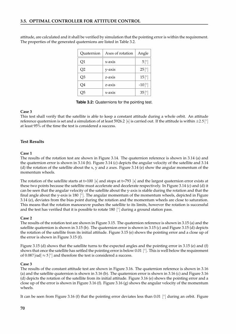
3.5. OPTIMAL CONTROLLER FOR ATTITUDE CONTROL
attitude, are calculated and it shall be verified by simulation that the pointing error is within the requirement.The properties of the generated quaternions are listed in Table 3.2.
Quaternion Axes of rotation Angle
Q1 x-axis 5 []
Q2 y-axis 25 []
Q3 z-axis 15 []
Q4 z-axis -10 []
Q5 x-axis 35 []
Table 3.2: Quaternions for the pointing test.
Case 3This test shall verify that the satellite is able to keep a constant attitude during a whole orbit. An attitudereference quaternion is set and a simulation of at least 5926.2 [s] is carried out. If the attitude is within±2.5 []at least 95% of the time the test is considered a success.
Test Results
Case 1The results of the rotation test are shown in Figure 3.14. The quaternion reference is shown in 3.14 (a) andthe quaternion error is shown in 3.14 (b). Figure 3.14 (c) depicts the angular velocity of the satellite and 3.14(d) the rotation of the satellite about the x, y and z axes. Figure 3.14 (e) show the angular momentum of themomentum wheels.
The rotation of the satellite starts at t=100 [s] and stops at t=793 [s] and the largest quaternion error exists atthese two points because the satellite must accelerate and decelerate respectively. In Figure 3.14 (c) and (d) itcan be seen that the angular velocity of the satellite about the y-axis is stable during the rotation and that thefinal angle about the y-axis is 180 []. The angular momentum of the momentum wheels, depicted in Figure3.14 (e), deviates from the bias point during the rotation and the momentum wheels are close to saturation.This means that the rotation manoeuvre pushes the satellite to its limits, however the rotation is successfuland the test has verified that it is possible to rotate 180 [] during a ground station pass.
Case 2The results of the rotation test are shown in Figure 3.15. The quaternion reference is shown in 3.15 (a) and thesatellite quaternion is shown in 3.15 (b). The quaternion error is shown in 3.15 (c) and Figure 3.15 (d) depictsthe rotation of the satellite from its initial attitude. Figure 3.15 (e) shows the pointing error and a close up ofthe error is shown in Figure 3.15 (f).
Figure 3.15 (d) shows that the satellite turns to the expected angles and the pointing error in 3.15 (e) and (f)shows that once the satellite has settled the pointing error is below 0.01 []. This is well below the requirementof 0.087 [rad]≈ 5 [] and therefore the test is considered a success.
Case 3The results of the constant attitude test are shown in Figure 3.16. The quaternion reference is shown in 3.16(a) and the satellite quaternion is shown in 3.16 (b). The quaternion error is shown in 3.16 (c) and Figure 3.16(d) depicts the rotation of the satellite from its initial attitude. Figure 3.16 (e) shows the pointing error and aclose up of the error is shown in Figure 3.16 (f). Figure 3.16 (g) shows the angular velocity of the momentumwheels.
It can be seen from Figure 3.16 (f) that the pointing error deviates less than 0.01 [] during an orbit. Figure
70

3.5. OPTIMAL CONTROLLER FOR ATTITUDE CONTROL
0
0.5
1
Rotation test results for the LQR controller
a) qref 1:4
−4−2
024
x 10−3
b) qerr 1:4
0
2
4
6x 10
−3
c) ωs
0
100
200
d) θatt
[°]
0 100 200 300 400 500 600 700 800 9000
0.5
1
1.5
x 10−4
e) Lmw
Figure 3.14: Test results for the rotation test. The x-axis is blue,the y-axis is green and the z-axis is red. The fourth quaternionelement is cyan.
3.16 (g) shows that the angular velocity of the momentum wheels deviate around the bias speed of 576 [rad/s]but they never saturate and they are thereby able to keep a stable attitude of the satellite. The deviation ofthe pointing error is well below the requirement of ±2.5 [] and therefore the test is considered a success.
71

3.5. OPTIMAL CONTROLLER FOR ATTITUDE CONTROL
0
0.5
1
Pointing test results for the LQR controller
a) qref 1:4
0
0.5
1 b) q
att 1:4
−0.4−0.2
00.20.4
c) qerr 1:4
−20
0
20
40
d) θatt
[°]
−40−20
02040
e) θerr
[°]
0 500 1000 1500 2000 2500
−0.02
0
0.02 f) θ
err[°]
Figure 3.15: Test results for the pointing test. The x-axis is blue,the y-axis is green and the z-axis is red. The fourth quaternionelement is cyan.
72

3.5. OPTIMAL CONTROLLER FOR ATTITUDE CONTROL
0
0.5
1
Constant attitude test results for the LQR controller
a) qref 1:4
0
0.5
1 b) q
att 1:4
−0.04−0.02
00.020.04
c) qerr 1:4
−20
0
20
40
d) θatt
[°]
−4−2
024
e) θerr
[°]
−0.02
0
0.02 f) θ
err[°]
0 1000 2000 3000 4000 5000 6000 7000 8000 9000 100000
500
1000 g) ω
mw[s−1]
Figure 3.16: Test results for the constant attitude test. The x-axis is blue, the y-axis is green and the z-axis is red. The fourthquaternion element is cyan.
73

3.6. DESATURATION CONTROLLER
3.6 Desaturation Controller
When the attitude of the satellite is controlled by the momentum wheels they will absorb disturbances actingon the satellite and eventually reach their saturation limit. When this happens, they will no longer be able tomaintain a stable attitude of the satellite. To avoid this, angular momentum must be moved from the satelliteto the inertial system, which in this case is the Earth, by applying an external torque with the magnetorquers.
3.6.1 Desaturation Strategy
There are different ways to desaturate the momentum wheels. Some of the possibilities are:
• Periodic B-dotThe momentum wheels are set to their bias speed and the B-dot controller is activated until the satellitehas been detumbled. This method will cause the satellite to spin and therefore it is not possible tocontrol the attitude while desaturating the momentum wheels.
• Continuous DesaturationDesaturation while maintaining attitude stability can be achieved with a magnetorquer controller thatminimizes the momentum wheel bias error. The attitude controller shall be activated while a biasminimizing controller desaturates the momentum wheels.
• Threshold DesaturationThis method is the same as continuous desaturation mentioned above, but it is only activated when thebias error rises above a certain turn-on level. The desaturation controller shall be deactivated when thebias error falls below a certain off-level. The two different levels and a Schmitt trigger are introducedin order to avoid fast on and off switching.
The threshold desaturation controller is chosen for the AAUSAT-II, because it can be used in pointing modeand it is only active when necessary and thereby it is preserving power.
3.6.2 Controller Design
The objective of the controller is to desaturate the momentum wheels. This is done by unloading angularmomentum, by the means of magnetic interaction with the Earth. By transferring angular momentum fromthe satellite to the Earth the bias error of the momentum wheels can be decreased. When the angular mo-mentum of the momentum wheels have deviated sufficient from their bias point the controller is activateduntil the bias error again is within an acceptable range.
It is not always possible to desaturate the momentum wheels because of the two axes control constraint ofthe magnetorquers. The torque from the magnetorquers acting on the satellite is given by
Nmt = mmt ×Bs, (3.52)
where mmt is the control input vector and Bs is the magnetic field of the Earth in the spacecraft frame.
The control law for the desaturation controller is given by
mmt = Cdesat(Lerr×Bs), (3.53)
where Lerr is the momentum wheel bias error given by
74

3.6. DESATURATION CONTROLLER
Lerr = Lwheel −Lwheel−bias. (3.54)
From (3.52) it can be seen that Nmt always lies in the normal plane to Bs. This means that only the part of Lerrthat is lying in the plane orthogonal to Bs, can be reduced by means of the magnetorquers. Therefore it isonly possible to fully desaturate the momentum wheels, when Lerr is orthogonal to Bs and it is not possibleto remove any angular momentum from the momentum wheels when Lerr is parallel to Bs.
If the desaturation controller is allowed to run while Lerr is parallel to Bs it will only introduce an error andconsume power, and none of these actions are beneficial for the satellite. However the amount of powerconsumed will be small because the magnitude of mmt is dependent on the angle between Bs and Lerr.
The supervisor that controls the desaturation controller shall use the part of Lerr that lies in the normal planeto Bs given by
lerr = ‖Lerr×Bs‖, (3.55)
in order to determine when to enable the desaturation controller. This will ensure that the controller only isenabled while it can remove angular momentum error from the momentum wheels. The SIMULINK imple-mentation of the desaturation controller and supervisor is shown in Figure 3.17.
4
d_on_off
3
m_mt
2
l_err
1
B_s1
s+1
Transfer Fcn2
1
s+1
Transfer Fcn1
1
s+1
Transfer Fcn
Switch
MATLABFunction
Supervisor control lawRelay
q(I−>S)
B(I)B(S)
Magnetic field I to S
Ground1
[q_I_S]From9
[Mag_I]From12
MATLABFunction
DesaturationControl law
5e9
C_desat1 L_err
Figure 3.17: SIMULINK implementation of desaturation controllerand supervisor.
3.6.3 Stability
The desaturation controller will render the system unstable if no stabilizing attitude controller is active andtherefore the attitude controller must be able to maintain a stable attitude while the momentum wheels aredesaturated.
3.6.4 Test
The desaturation controller has been tested with the LQR controller in SIMULINK with these parameters:
Cdesat = 5 ·107
lerr on = 2 ·10−11
lerr off = 7 ·10−11
Lbias = [7.96 7.96 7.96] ·10−6 [kgm2/s]
75

3.6. DESATURATION CONTROLLER
The test results can be seen in Figure 3.18
During the test some manoeuvres have been simulated as can be seen from the attitude quaternion in Figure3.18 (a) and 3.18 (b). Figure 3.18 (c) shows the angular velocity of the momentum wheels and Figure 3.18(d) shows the angular velocity of the satellite. In Figure 3.18 (e) and 3.18 (f) the torque applied from themagnetorquers and the angular momentum error in the momentum wheels are shown. Figure 3.18 (g) showsthe norm of the error that can be desaturated and Figure 3.18 (h) shows the on/off signal to the desaturationcontroller.
From Figure 3.18 it can be seen that the desaturation controller desaturates the momentum wheels after eachmanoeuvre. The supervisor shuts off the desaturation controller when no more angular momentum canbe removed from the wheels and this can be seen at t=90 [s] and t=800 [s] where the magnitude of Lerr isdifferent at shut-off time. From t=800 [s] and forward no more manoeuvres are carried out and it is shownthat the desaturation controller is activated briefly at t=850 [s] and t=940 [s] because it is possible to removemore angular momentum. This shows that the desaturation controller will keep the error at a minimum andthereby enable the LQR controller to keep the satellite stable over longer periods of time.
76

3.6. DESATURATION CONTROLLER
−0.2
0
0.2
0.4
Test results for the desaturation controller
a) qatt 1:3
0.9
0.95
1 b) q
att 4
0200400600800
c) ωmw
−0.02
0
0.02
0.04 d) ω
s
−10
−5
0
5
x 10−7
e) Nmt
−5
0
5
x 10−5
f) Lerr
0
1
2
3
x 10−9
g) lerr
0 100 200 300 400 500 600 700 800 900 1000
0
0.5
1 h) d
on−off
Time [s]
Figure 3.18: Test results from the desaturation controller withthe LQR controller. The x-axis is blue, the y-axis is green and thez-axis is red.
77

Conclusion 4This report concerns the development of the attitude control system for AAUSAT-II. Requirements havebeen outlined and the satellite and space environment have been modelled in SIMULINK. These assignmentshave been made in collaboration with the attitude determination system team, group 05GR833. Based onthese models, different controllers have been developed which together constitute a complete ACS systemwhich enables the satellite to detumble and do pointing manoeuvres. The controllers have been tested in theSIMULINK simulation environment.
System demands for the ADCS system have been outlined in Section 1.5 on page 12. These demands concern:
• Detumbling below 0.0021 [rad/s] within three orbits.
• Maintaining an average minimum angular velocity of 0.0045 [rad/s] during an overflight of the groundstation.
• Maintaining a given attitude within 0.087 [rad].
• Implementation such that new controller algorithms may be uploaded.
These demands are to be fulfilled by the overall ADCS system, but have been applied to the ACS systemalone, since the ADS system and the ACS system have not yet been integrated.
In collaboration with the ADS team, group 05GR833, a model of the environment for the satellite have beendeveloped, including the spacecraft dynamics and kinematics. Different reference frames have been definedin order to reduce the complexity of the model and computational power needed to run the ADCS system on-board the satellite. A simulation library, containing the satellite and space environment has been developedin SIMULINK. It contains both satellite sensors and actuators, but since the ACS system does not use thesensors directly, the modelling of those have been left out of this report. The simulation environment containsdisturbances in space and parts of the model have been made generic, offering the possibility of simulatingthe behaviour of other satellites.
Only verification of the orbit model and the magnetic field model has been conducted. Verifications of theother simulation models have not been carried out, because reliable test methods are hard to find. No testdata of the satellite in orbit is available and hence there is no data to test the model up against.
A supervisor for managing the controllers of the attitude control system has been designed in order to switchbetween detumbling mode and pointing mode. The supervisor also detects if the angular velocity of thesatellite increases in pointing mode, and switches to detumbling mode if it does, to ensure the safety of thesatellite.
A detumbling controller, based on the B-dot algorithm has been designed to make the satellite follow themagnetic field of the Earth. The detumbling controller is designed as a simple and robust controller toincrease the possibility of being able to detumble the satellite after deployment from the launch vehicle.Tests of the B-dot controller indicate that it is capable of reducing the angular velocity of the satellite below0.0021 [rad/s] within the specified three orbits. It is able to detumble the satellite within approximately oneorbit and hence performs better than expected.
An optimal controller was designed for the momentum wheels to control the attitude of the satellite. To keep
78

4.1. FUTURE WORK
the momentum wheels from reaching their limits of angular velocity, a supervisor to control the desaturationof the momentum wheels, has been designed. This composition provides the pointing controller for thesatellite. Tests show that the pointing controller is capable of maintaining a given attitude of the satellitewithin 0.087 [rad]. Furthermore the pointing controller is capable of maintaining an average angular velocityof minimum 0.0045 [rad/s] which is necessary in order to be able to point the antennas towards the groundstation during an ideal overflight.
The tests of the controllers imply that the attitude of the satellite may be controlled using the designed con-trollers. Though the controllers have not yet been implemented on the satellite, as no hardware is completeyet. Furthermore the ACS also requires testing with the ADS and the ADCS hardware teams before it can beverified if the complete ADCS system meets the demands. Even if ACS and ADS alone are able to fulfil thesystem demands for ADCS, there is no guarantee that the systems combined are stable as they depend oneach other. Therefore the complete ADCS requires combined testing before implementation on the satellite.
4.1 Future Work
Before the ACS may be considered finished, some improvements need to be implemented. The detumblingcontroller has been tested while switching the magnetorquers on and off to be able to use the magnetometersfor measuring the magnetic field. This feature needs to be implemented on the desaturation controller aswell.
When the controllers have been tuned and implemented to fulfil all requirements from the hardware, thecontrollers may be implemented on the satellite. This requires the models in SIMULINK to be ported to theon-board computer on the satellite. After implementation it needs to be tested if new controllers can beuploaded to the ADCS system, in order to fulfil the last statement of the system demands.
79

BIBLIOGRAPHY
Bibliography
[04GR830a] Group 04GR830a Aalborg University. Attitude Control System for AAUSAT-II. 2004./doc/ACS04.pdf on the enclosed CD-ROM.
[04GR830b] Group 04GR830b Aalborg University. Attitude Determination System for AAUSAT-II.2004. /doc/ADS04.pdf on the enclosed CD-ROM.
[ADS05] Group 05GR833 Aalborg University. Attitude Determination System for AAUSAT-II.2005. /doc/ADS05.pdf on the enclosed CD-ROM.
[Anderson et al.] Dennis J. Sweeney David R. Anderson and Thomas A. Williams. Modern BusinessStatistics with Microsoft Excel. South Western, 2003. ISBN 0-324-12174-1.
[Bhanderi] Dan Bhanderi. Spacecraft Attitude Determination with Albedo Corrected Sun Sensor Mea-surements., 2005. Not Published.
[Braeunig] Robert Braeunig. Orbital Mechanics, 2005. http://www.braeunig.us/space/orbmech.htm.
[Chou] IEEE Transactions on Robotics and Automation. Quaternion kinematic and dynamicdifferential equations. Jack C. K. Chou. nr. 1. February 1992. side 53 –64.
[COM] Group 05GR834 Aalborg University. The AAUSAT-II Communication System. 2005./doc/com.pdf on the enclosed CD-ROM.
[CubeSat ACS] Michael Kvist Frederiksen Torben Graversen and Søren Vejlgaard Vedstesen. Atti-tude Control System for AAU CubeSat. 2002. /doc/cubesat-ACS.pdf on the enclosedCD-ROM.
[CubeSat ADS] Kristian Krogh and Elmo Schreder. Attitude Determination for AAU CubeSat. 2002./doc/cubesat-ADS.pdf on the enclosed CD-ROM.
[Franklin et al.] Michael Workman Gene F. Franklin, J. David Powell. Digital Control of Dynamic Sys-tems. Addison Wesley Longman, Inc., 1998. ISBN 0-201-82054-4.
[MECH-WWW] Mechanical group of AAUSAT-II. "Mechanical System - AAUSAT-II", May17th 2005. http://www.aausatii.auc.dk/wiki/index.php/Mechanical_System /doc/satellite-frame.jpg on the enclosed cd.
[IAGA V-MOD] IAGA V-MOD Working Group. IAGA V-MOD Geomagnetic Field Modeling: In-ternational Geomagnetic Reference Field IGREF-10, Downloaded May 2005. http://www.ngdc.noaa.gov/IAGA/vmod/igrf.html.
[ADCS HW ICD] ADCS Hardware. ADCS Hardware ICD, May 2005. /doc/adcs-icd.txt on the enclosedCD-ROM.
[Hmnao] Hmnao. The Astronomical Almanac for the Year 2003. The Stationery Office, 2003. ISBN0-11-887320-2.
[Hoots & Roehrich] Felix R. Hoots and Ronald L. Roehrich. SPACETRACK REPORT NO. 3 - Modelsfor Propagation of NORAD Element Sets, 1980. http://celestrak.com/NORAD/documentation/spacetrk.pdf /doc/spacetrk.pdf on the enclosed CD-ROM.
80

BIBLIOGRAPHY
[Hughes] Peter C. Hughes. Spacecraft Attitude Dynamics. Wiley and Sons, Inc, 1986. ISBN0-471-81842-9.
[Kelso] T. S. Kelso. Frequently Asked Questions: Two-Line Element Set Format, 1998. http://celestrak.com/columns/v04n03/.
[Kuipers] Jack B. Kuipers. Quaternions and Rotation Sequences: A Primer with Applications toOrbits, Aerospace, and Virtual Reality. Princeton University Press, 2002. ISBN 0-691-10298-8.
[MECH-Mail] MECH. Email from MECH concerning the inertia matrix of the satellite., 2005. /doc/in-ertia_mech.pdf on the enclosed CD-ROM.
[Maxon RE10] Maxon Motor. Maxon DC motor RE 10 data sheet, April 2005. http://www.maxonmotor.com/docsx/Download/catalog_2005/Pdf/05_053_e.pdf/datasheets/Maxon_RE-10.pdf on the enclosed CD-ROM.
[NASA/GSFC] Ozone Processing Team NASA/GSFC Code 916. Total Ozone Mapping Spectrometer.NASA and Goddard Space Flight Center, Downloaded April 2005. http://toms.gsfc.nasa.gov.
[Powell et al.] J. David Powell Gene Franklin and Abbas Emami-Naeini. Feedback Control of Dyna-mic Systems. Prentice-Hall, Inc., 2002. ISBN 0-13-098041-2.
[LM628] National Semiconductor. LM628/LM629 Precision Motion Controller, DownloadedMarch 2005. http://www.national.com/ds.cgi/LM/LM628.pdf /datasheet-s/LM628.pdf on the enclosed CD-ROM.
[Serway & Beichner] Raymond A. Serway and Robert J. Beichner. Physics For Scientists and Engineers withModern Physics. Harcourt College Publishers, 2000. ISBN 0-03-022657-0.
[Sidi] Marcel J. Sidi. Spacecraft Dynamics and Control. Cambridge University Press, 1997.ISBN 0-521-55072-6.
[Space Track] Space-Track.Org. Space Track - The Source for Space Surveillance Data, DownloadedApril 2005. http://www.space-track.org.
[BGS] British Geological Survey. An Overview of the Earth’s Magnetic Field, DownloadedMay 2005. http://www.geomag.bgs.ac.uk/earthmag.html.
[Princeton] Princeton Satellite Systems. Princeton Satellite Systems, moonV2.m, 1993. /aausatii-sim/lib/space_environment_emulation/ephemeris/MoonV2.m on the enclosedCD-ROM.
[Optimal] Ole Sørensen. Introduction to Optimal Control, August 1995. /doc/optimalcontrol.pdfon the enclosed CD-ROM.
[CPSU] California Polytechnic State University. CubeSat Program, 2005. http://cubesat.calpoly.edu/_new/index.html.
[Weisstein Cofactor] Eric W. Weisstein. Cofactor, Downloaded March 2005. http://mathworld.wolfram.com/Cofactor.html.
[Weisstein Ellipse] Eric W. Weisstein. Ellipse, Downloaded March 2005. http://mathworld.wolfram.com/Ellipse.html.
[Wertz & Larson] James R. Wertz and Wiley J. Larson. Space Mission Analysis. Microcosm Press andKluwer Academic Publishers, 1999. ISBN 1-881883-10-8.
[Wertz] James R. Wertz. Spacecraft Attitude Determination and Control. Kluwer AcademicPublishers, 1978. ISBN 90-277-0959-9.
[Wie] Bong Wie. Space Vehicle Dynamics and Control. American Institute of Aeronautics andAstronautics, Inc, 1998. ISBN 1-56347-261-9.
[Wisniewski] Rafał Wisniewski. Satellite Attitude Control Using Only Electromagnetic Actuation. De-partment of Control Engineering, Aalborg University, 1996. /doc/Wisniewski.pdfon the enclosed CD-ROM.
81

Quaternions ASince the kinematics of the satellite are best expressed in quaternion form for calculation purposes this ap-pendix includes quaternion definitions and describes the fundamental algebraic properties of quaternions.As sources for this appendix [Wertz, page 758-759] and [Chou] are used.
A.1 Quaternion Definitions
A quaternion is a hyper complex number and can be defined as
q = iq1 + jq2 + kq3 +q4, (A.1)
where the hyperimaginary numbers i, j and k satisfy the following conditions
i2 = j2 = k2=−1
i j = − ji = k
jk = −k j = i
ki = −ik = j. (A.2)
In (A.1) the parameter q4 is also known as the real part or the scalar part. The first three terms in (A.1) arenormally denoted the imaginary part or vector part. By defining the vector part as
q1:3 = iq1 + jq2 + kq3, (A.3)
it is possible to make the following representation of (A.1)
q = (q1:3,q4). (A.4)
When quaternions are used for attitude descriptions and generally for rotation of objects the four parameters(q1,q2,q3,q4) are defined as
q1 = e1 sin(θ/2) (A.5)q2 = e2 sin(θ/2) (A.6)q3 = e3 sin(θ/2) (A.7)q4 = cos(θ/2). (A.8)
where e21 + e2
2 + e23 = 1 which implies that ‖q‖ = 1 and further that the use of this subset of quaternions
performs rotations while preserving lengths.
The difference between two quaternions, i.e. the attitude error can be calculated as
82
A.2. QUATERNION ALGEBRA
qerr = qatt q−1ref , (A.9)
where qatt is the calculated attitude quaternion and qref is the reference attitude quaternion given by thedynamics and kinematics of the satellite.
A.2 Quaternion Algebra
The fundamental mathematical operations that will be described in this section are addition and subtractionof quaternions, the norm and inverse of quaternions and multiplication of quaternions.
A.2.1 Addition and Subtraction
The addition and subtraction of quaternions obey the associative and commutative laws and are defined as
qA±qB = (qA1:3±qB1:3)+(qA4±qB4). (A.10)
Quaternions are added and subtracted as normal complex numbers or vectors.
A.2.2 Norm and Inverse
The norm of a quaternion is calculated like the norm of a complex number and is defined as
‖q‖=√
q21 +q2
2 +q23 +q2
4. (A.11)
The inverse of a quaternion is defined as
q−1 =q∗
‖q‖, (A.12)
where q∗ is the complex conjugate of q, which is defined as
q =−iq1− jq2− kq3 +q4 = (−q1:3 +q4). (A.13)
From (A.12) it should be noticed that when the norm of a quaternion is 1 the inverse of that quaternion isequal to the complex conjugate of that same quaternion.
A.2.3 Multiplication
Quaternion multiplication is performed in the same way as multiplication of complex numbers. However,the order of operation must be taken into account as quaternion multiplication does not obey the commuta-tive law, i.e., qAqB 6= qBqA.
The following expression defines the multiplication of two quaternions qA and qB.
83

A.2. QUATERNION ALGEBRA
qC = qAqB = (qA4 + iqA1 + jqA2 + kqA3)(qB4 + iqB1 + jqB2 + kqB3). (A.14)
Using (A.2) it is possible to express (A.14) as
qC = qAqB = i(qA1 qB4 +qA2qB3 −qA3 qB2 +qA4qB1)+ j(−qA1 qB3 +qA2qB4 +qA3 qB1+qA4 qB2
)
+k(qA1 qB2 −qA2qB1 +qA3 qB4 +qA4qB3)+(−qA1qB1 −qA2 qB2 −qA3qB3 +qA4 qB4). (A.15)
In matrix form (A.15) becomes
qC1
qC2
qC3
qC4
=
qB4 qB3 −qB2 qB1
−qB3 qB4 qB1 qB2
qB2 −qB1 qB4 qB3
−qB1 −qB2 −qB3 qB4
qA1
qA2
qA3
qA4
. (A.16)
Given two successive rotations qA and qB, (A.16) gives the components of the quaternion that describes thecombined rotation.
84

Rotations BThis appendix explains different rotation methods such as the direction cosine matrix denoted attitude ma-trix, Euler angles and Eulers eigenaxis rotation theorem. Furthermore, this appendix deals with the deriva-tion of the kinematic differential equation for the attitude matrix. This appendix is based on [Kuipers]and [Wie, pages 307-329].
B.1 Direction Cosine
In the following two reference frames will be used, A and B, which are both right handed and have basesformed by the orthogonal sets of unit vectors (a1, a2, a3) and (b1, b2, b3) respectively. A rotation matrixtransforming A into B can be found by expressing the basis of B in terms of A
b1 = C11a1 +C12a2 +C13a3 (B.1)b2 = C21a1 +C22a2 +C23a3 (B.2)b3 = C31a1 +C32a2 +C33a3. (B.3)
(B.1), (B.2) and (B.3) can be written in matrix notation as
b1
b2
b3
=
C11 C12 C13
C21 C22 C23
C31 C32 C33
a1
a2
a3
= BAC
a1
a2
a3
, (B.4)
where BAC is called the attitude matrix as each element is calculated by projection,
BAC =
b1 · a1 b1 · a2 b1 · a3
b2 · a1 b2 · a2 b2 · a3
b3 · a1 b3 · a2 b3 · a3
, (B.5)
where BACi j = bi · a j = cos(αi j) as the basis1 of A and B consists of unit vectors and αi j is the angle between
the two elements. Analogously the rotation from B to A can be found as
a1
a2
a3
= ABC
b1
b2
b3
, (B.6)
1Hence the commonly used notion direction cosine matrix.
85

B.2. EULER ANGLES
where
ABC =
a1 · b1 a1 · b2 a1 · b3
a2 · b1 a2 · b2 a2 · b3
a3 · b1 a3 · b2 a3 · b3
. (B.7)
B.2 Euler Angles
There exist three special forms of the attitude matrix which each rotates the reference frame about one of itsaxes - these are called elementary rotations.
Rotation around the third axis as depicted in Figure B.1
θ3
a1 − axis
a2 − axisb2 − axis
b1 − axis
Figure B.1: Example of Euler rotation around the z-axis
yields the transformation matrix
C3 =
b1 · a1 b1 · a2 b1 · a3
b2 · a1 b2 · a2 b2 · a3
b3 · a1 b3 · a2 b3 · a3
. (B.8)
The two reference frames have the same third-axis and the three axes are orthogonal, hence b1 · a3 = b2 · a3 =b3 · a1 = b3 · a2 = 0 and b3 · a3 = 1 This yields
C3 =
b1 · a1 b1 · a2 0
b2 · a1 b2 · a2 0
0 0 1
. (B.9)
The remaining dot products can be calculated by inspecting the projection of a1 and a2 on the b1 and b2 unitvectors which yields
C3 =
cos(θ3) sin(θ3) 0
−sin(θ3) cos(θ3) 0
0 0 1
. (B.10)
86

B.3. EULER’S EIGENAXIS ROTATION THEOREM
Similar calculations for the second- and first-axis yields
C2 =
cos(θ2) 0 −sin(θ2)
0 1 0
sin(θ2) 0 cos(θ2)
and C1 =
1 0 0
0 cos(θ1) sin(θ1)
0 −sin(θ1) cos(θ1)
. (B.11)
Note that the sign of the sine terms are opposite when rotating about the second axis, due to the propertiesof the righthanded reference frame.
By combining three of the Euler rotations, without having two successive rotations around the same axis, itis possible to obtain an arbitrary rotation. Thus, there exists 12 possible sets of Euler rotations.
B.3 Euler’s Eigenaxis Rotation Theorem
Euler’s eigenaxis rotation theorem uses a vector fixed in one reference frame during rotation rather thanone of the axes. Consider a reference frame B rotated an angle of θ around a unit vector e to coincide withreference frame A,
e = e1a1 + e2a2 + e3a3 (B.12)= e1b1 + e2b2 + e3b3. (B.13)
As e is fixed in reference frame A, (B.12) and (B.13) can be expressed as an attitude matrix,
e1
e2
e3
=
C11 C12 C13
C21 C22 C23
C31 C32 C33
e1
e2
e3
= C
e1
e2
e3
. (B.14)
The rotation matrix C can be expressed as three successive rotations. First A is rotated to the point where theunit vector a1 is aligned with e thus constructing a new reference frame A’. This is done using the rotationmatrix
R =
e1 e2 e3
R21 R22 R23
R31 R32 R33
. (B.15)
Second the reference frames A and A’ are rotated around e by an angle of θ. After this rotation the A framewill be aligned with the B frame and A’ will construct a new reference frame A” via the rotation matrix
A”A’ C =
1 0 0
0 cosθ sinθ
0 −sinθ cosθ
. (B.16)
It is important to notice that the relative rotation of B to A” is equal to the rotation from A to A’ i.e. A”B C =
A’AC = R.
87

B.4. ATTITUDE MATRIX AND KINEMATICS
The third of the three successive rotations needs to align the reference frame A” with B. This is done byrotating A” through an inverse matrix R−1 = RT since B
A”C = R−1. It is now possible to describe the rotationfrom A to B by the attitude matrix B
AC expressed as
BAC = B
A”CA”A’ C
A’AC. (B.17)
By inserting (B.15) and (B.16) in (B.17) the elements of the matrix BAC can be expressed as
C11 = e21 +(R2
21 +R231)cos(θ)
C12 = e1e2 +(R21R22 +R31R32)cos(θ)+(R21R32−R22R31)sin(θ)C13 = e1e3 +(R21R23 +R31R33)cos(θ)+(R21R33−R23R31)sin(θ)
... (B.18)C33 = e2
3 +(R223 +R2
33)cos(θ).
Utilizing the orthonormality condition RT R = I, yields
e21 +R2
21 +R231 = 1
e22 +R2
22 +R232 = 1
e23 +R2
23 +R233 = 1
e1e2 +R21R22 +R31R32 = 0e2e3 +R22R23 +R32R33 = 0e1e3 +R21R23 +R31R33 = 0,
and calculating the cofactor of each of the elements (e1,e2,e3) [Weisstein Cofactor],
e1 = R22R33−R32R23
e2 = R23R31−R21R33
e3 = R21R32−R31R22,
it is possible to obtain the rotation matrix
BAC =
cθ+ e2
1(1− cθ) e1e2(1− cθ)+ e3sθ e1e3(1− cθ)− e2sθ
e2e1(1− cθ)− e3sθ cθ+ e22(1− cθ) e2e3(1− cθ)+ e1sθ
e3e1(1− cθ)+ e2sθ e3e2(1− cθ)− e1sθ cθ+ e23(1− cθ)
, (B.19)
where cθ≡ cos(θ), sθ≡ sin(θ) and ei are the direction cosines of the Euler axis. The parameters (e1,e2,e3) arenot independent but constrained by e2
1 + e22 + e2
3 = 1.
B.4 Attitude Matrix and Kinematics
In order to derive the kinematic differential equation, two reference frames, A and B, are used. A timevarying angular velocity vector in the reference frame B is denoted as ω. This vector can also be expressedin terms of the unit vectors of reference frame B which yields
ω = ω1b1 + ω2b2 + ω3b3. (B.20)
88

B.4. ATTITUDE MATRIX AND KINEMATICS
In (B.4) the attitude matrix C = BAC was defined such that
b1
b2
b3
= C
a1
a2
a3
. (B.21)
Because the attitude matrix C is an orthonormal matrix (B.21) can be rewritten to the following
a1
a2
a3
= CT
b1
b2
b3
. (B.22)
Since the two reference frames, A and B, are rotating relative to each other then the attitude matrix and itselements Ci j are time dependent. Taking the time derivative of (B.22) in A yields the following equation
0
0
0
= CT
b1
b2
b3
+CT
˙b1˙b2˙b3
. (B.23)
Because the unit vectors bi are fixed in reference frame B are rotating relative to A, the rate of change in bi isonly caused by ω. This means that the time derivative of the unit vector ˙bi, must be normal to both bi and ω.Thus (B.23) can be expressed as
0
0
0
= CT
b1
b2
b3
+CT
ω× b1
ω× b2
ω× b3
. (B.24)
By introduction of the skew symmetric matrix
S(ω) = ωT ×ω =−ω×ω
T =−
ω1
ω2
ω3
×[ω1 ω2 ω3
]
≡ −
ω1× ω1 ω1× ω2 ω1× ω3
ω2× ω1 ω2× ω2 ω2× ω3
ω3× ω1 ω3× ω2 ω3× ω3
(B.25)
=
0 −ω3 ω2
ω3 0 −ω1
−ω2 ω1 0
, (B.26)
it is possible to substitute the cross product in (B.24) with a multiplication [Hughes, page 524], and rewrite(B.23) to
89

B.4. ATTITUDE MATRIX AND KINEMATICS
0
0
0
=[
CT −CT S(ω)]
b1
b2
b3
, (B.27)
which is again rewritten to0 = CT −CT S(ω). (B.28)
By transposing both sides of (B.27) and utilizing the relationship ST (ω) =−S(ω) the following expression isobtained
0 = C+S(ω)C. (B.29)
This expression is the kinematic differential equation for the direct cosine matrix.
90

Two Line Elements CWhen the satellite has been deployed an initial position of the satellite must be obtained for use in the on-board model. The North American Aerospace Defense Command (NORAD) tracks objects that orbit theEarth. Data concerning the orbit of these objects e.g. Keplerian elements, are distributed using Two LineElements (TLE), which can be obtained free of charge [Space Track] and are updated on a daily basis. A TLEcan thus be used to initialize the orbit model.
A TLE has the following format:
AAAAAAAAAAAAAAAAAAAAAAAAAAAAAAAA1 BBBBBC DDEEEFFF GGHHH.HHHHHHHH +.IIIIIIII +JJJJJ-J +KKKKK-K L MMMMN2 BBBBB OOO.OOOO PPP.PPPP QQQQQQQ RRR.RRRR SSS.SSSS TT.TTTTTTTTUUUUUN
Each of the elements in the TLE denoted by the letters are described in Table C.1, and an example of a TLEfrom the AAU CubeSat can be seen below:
AAU CUBESAT1 27846U 03031G 04070.99002110 -.00000777 00000-0 -34070-3 0 17202 27846 98.7298 79.6436 0008339 275.9042 84.1157 14.20604785 36102
In the following the elements of the TLE are described further based on [Kelso]. Referring to Table C.1, theelements A through F are used to identify the object to which the TLE is related. Elements G and H define thereference time for the element set and are jointly referred to as the epoch. Elements I and J are primarilyused in older orbit models such as the SGP model, and are not used in the SGP4 model. The perturbationsmodelled by the SGP4 model include aerodynamic drag where element K is a coefficient. Element L isrelated to the model (i.e. SGP/SGP4) used for generating the TLE. The element is used internally only, andall distributed TLEs have the element set to zero. The element M is used for keeping track of the receivednumber of TLEs and the value is increased each time a new TLE is generated.
The elements O through R have been described in Section 2.1.1. Element S, the mean anomaly is defined byM = 2π
(∆tP
), where P is the orbital period and ∆t is the time since perigee passage of the satellite. Element U
has the following definition: A revolution begins when the satellite is at the ascending node of the orbit anda revolution is the period between successive ascending nodes. The period from launch to the first ascendingnode is considered to be revolution 0 and revolution 1 begins when the first ascending node is reached.
Element N is used for checksum on each line and represents a modulo-10 checksum of the data on the currentline. To calculate the checksum the values of all the numbers must be added on each line. All letters, spaces,periods, and plus signs are ignored, and all minus signs are assigned the value 1.
91

Element Description
A Satellite name
1 Line 1 of element data
B Satellite number
C Classification (U=Unclassified)
D Last two digits of launch year
E Launch number of the year
F Item number of the launch
G Last two digits of epoch year
H Epoch day and fractional portion of the day
I First time derivative of the mean motion [m/s2]
J Second time derivative of the mean motion [m/s3]
K BSTAR drag term
L Ephemeris type
M Element number
N Checksum
2 Line 2 of element data
O Inclination []
P RAAN []
Q Eccentricity (Decimal point assumed)
R Argument of perigee []
S Mean anomaly []
T Mean motion [Revolutions per day]
U Revolution number at epoch
N Checksum
Table C.1: The format of a Two Line Element.
92

Linearization DFrom Equation 2.74 on page 41 the system equations are given. In order to use the system equations e.g. foroptimal control or a Kalman Filter, these nonlinear equations have to be linearized. The satellite kinematicsand dynamics equations are given by
ω
q
=
I−1(Next +Ncrtl−S(ω)(Iω+Lmw))12 Ωq
. (D.1)
A linear description of the satellite attitude will be found by linearizing (D.1) about an operating point.Thereby the satellite dynamics and kinematics can be expressed in state space.
D.1 Linearization of the Satellite Kinematic Equation
The satellite kinematic equation is expressed as
q =12
Ωq. (D.2)
Linearizations of quaternions are used in order to linearize (D.2). The quaternion can then be expressed as
q = q(t +∆t) = q(t)q(∆t) = qq, (D.3)
where q is the quaternion in the operating point q(t) and q is the small signal quaternion, q(∆t), representinga small change in attitude. Using the fact that q−1 = q∗, then q can be derived from (D.3) as
q = q∗q, (D.4)
where q∗ is the complex conjugate of q.
It is possible to rewrite the kinematic equation of the satellite in (D.2) into a multiplication of two quaternions,using the multiplicational properties of a quaternion as expressed in (D.5). The result can be seen in (D.6).
93

D.1. LINEARIZATION OF THE SATELLITE KINEMATIC EQUATION
qqω = (q4 +q1 i+q2 j +q3k) · (0+ω1 i+ω2 j +ω3k)
=
0 ω3 −ω2 ω1
−ω3 0 ω1 ω2
ω2 −ω1 0 ω3
−ω1 −ω2 ω3 0
︸ ︷︷ ︸
Ω
q1
q2
q3
q4
︸ ︷︷ ︸
q
, (D.5)
q =12
qqω, (D.6)
where qω is defined as
qω =
ω3×1
0
=
ω3×1 + ω3×1
0
= qω +qω. (D.7)
In the following calculations the properties of the complex conjugate of the quaternion (qqω)∗ = q∗ωq∗ andq∗
ω=−qω will be used as the scalar part of qω is zero. Taking the derivative of (D.4) with respect to time and
utilizing (D.6), yields
˙q = ˙q∗q+ q∗q
=12
[(qqω)∗q+ q∗(qqω)]
=12
[(qqω)∗ q+ qqω
]=
12
[q∗ωq∗q+ qqω]
=12
[−qωq+ qqω] . (D.8)
Inserting (D.7) into (D.8) yields
˙q =12
[−qωq+ qqω]
=12
[−qωq+ qqω + qqω]
=12
[−qωq+ qqω]+12
qqω. (D.9)
Calculating the quaternion products qωq in (D.9) yields
qωq =
−S(q1:3)+ q413×3 q1:3
−qT1:3 q4
ω
0
=
S(ω)q1:3 + q413×3ω
−qT1:3ω
. (D.10)
94

D.1. LINEARIZATION OF THE SATELLITE KINEMATIC EQUATION
Note that S(ω) is the skew symmetric matrix described in Equation 2.53 on page 38 and that S(ω)q =−S(q)ω.The multiplication of qqω can be found as follows
qqω =
−S(ω) ω
−ωT 0
q1:3
q4
=
−S(ω)q1:3 + ωq4
−ωT q1:3
. (D.11)
Finally the multiplication of qqω must be derived. In this case note that each quaternion represents a rotationand it has a vector part, q1:3, with dimensions 3×1 and a scalar part (q4). Therefore small rotations yields.
limrotation→0
q = limθ→0
q1:3
q4
= limθ→0
e1 sin
(θ
2
)e2 sin
(θ
2
)e3 sin
(θ
2
)cos
(θ
2
)
=
q1:3 → 0
q4 → 1(D.12)
Therefore qqω can be approximated with qω as shown in (D.13).
qqω =
−S(ω) ω
−ωT 0
q1:3
q4
=
−S(ω)q1:3 + ωq4
−ωT q1:3
≈
0+
ω1
ω2
ω3
0
q4
0
=
ω1
ω2
ω3
0
= qω. (D.13)
Now it is possible to substitute the results of (D.10), (D.11) and (D.13) into (D.9), yielding the following linearexpression for the kinematics of the satellite.
˙q =12
− S(ω)q1:3 + q413×3ω
−qT1:3ω
+
−S(ω)q1:3 + q413×3ω
−ωT q1:3
+12
qqω
=
−S(ω)q1:3
0
+12
qqω
≈
−S(ω)q1:3
0
+12
qω. (D.14)
as the aT b = bT a applies.
95

D.2. LINEARIZATION OF SATELLITE DYNAMIC EQUATION
D.2 Linearization of Satellite Dynamic Equation
The satellite dynamic equation is stated in Equation 2.74 on page 41 as
ω = I−1[Next +Nctrl−S(ω)(Iω+Lmw)]. (D.15)
To linearize the dynamic equation, it is necessary to choose an operating point ω for the system. The ope-rating point varies in different time steps but is constant in each specific time step. The change in angularvelocity is modelled with the small signal ω in the operating point. This yields
ω = ω(t +∆t) = ω+ ω. (D.16)
The derivative of (D.16) with respect to time yields
ω = ˙ω. (D.17)
Taking (D.15) into consideration it is possible to assume Next as constant about the operating point withinthe time frame ∆t. Therefore, ω becomes a function of ω, Nctrl and Lmw. (D.15) is linearized using first orderTaylor expansion.
ω(ω,Lmw,Nctrl) ≈ −I−1 ddω
S(ω)(Iω+Lmw)∣∣∣∣ω=ω,Lmw=Lmw
· ω
− I−1 ddLmw
S(ω)(Iω+Lmw)∣∣∣∣ω=ω,Lmw=Lmw
· Lmw
+ I−1 ddNctrl
Nctrl
∣∣∣∣Nctrl=Nctrl
· Nctrl. (D.18)
By rewriting the ω term and expanding the Nctrl and Lmw terms, (D.18) can be expressed in the form
ω = −I−1[
ddω
S(ω)Iω∣∣∣∣ω=ω
+d
dωS(ω)Iω
∣∣∣∣ω=ω
+d
dωS(ω)Lmw
∣∣∣∣ω=ω
]ω
− I−1 ddLmw
S(ω)Lmw
∣∣∣∣ω=ω,Lmw=Lmw
· Lmw + I−1Nctrl. (D.19)
Using the fact that S(ω)Iω =−S(Iω)ω then (D.19) can be expressed as
ω = I−1[
ddω
S(Iω)ω∣∣∣∣ω=ω
− ddω
S(ω)Iω∣∣∣∣ω=ω
+d
dωS(Lmw)ω
∣∣∣∣ω=ω
]ω
−I−1S(ω)Lmw + I−1Nctrl. (D.20)
From (D.20) the linearized dynamic differential equation shown in (D.21) is obtained as
ω = I−1 [S(Iω)−S(ω)I+S(Lmw)] ω− I−1S(ω)Lmw + I−1Nctrl. (D.21)
96

D.3. LINEAR EQUATION FOR THE SATELLITE ATTITUDE
D.3 Linear Equation for the Satellite Attitude
Using the results given in the two previous sections, it is possible to obtain the linear system equation for thesatellite, which is expressed as
˙q1:3
ω
˙Lmw
=
−S(ω) 1
2 13×3 03×3
03×3 I−1 [S(Iω)−S(ω)I+S(Lmw)] −I−1S(ω)
03×3 03×3 03×3
q1:3
ω
Lmw
+
03×3 03×3
I−1 −I−1
03×3 13×3
Nmt
Nmw
. (D.22)
Note that in this equation the scalar element of the quaternion, q4, does not yield a contribution as it isapproximated to be 1 for small angles. See (D.12). S(ω) and S(Lmw) are constant in their operating pointsand they are calculated in each operating point using the measurements from the gyros and the tachometerson the momentum wheels. Nmt and Nmw are small changes in the torques exerted by the actuators withinthe ∆t time frame.
97

Implementation of Simulation EThe models deducted in the report have all been implemented in MATLAB and SIMULINK to be able to testthe ADCS system. In the following chapter the implementation of the different models will be presented.The implementation is based on the work done by group 04gr830a [04GR830a] and 04gr830b [04GR830b],Aalborg University. The implementation is available on the enclosed CD.
E.1 Simulation Environment
This section presents the implementation of the models related to the simulation environment.
E.1.1 Disturbance Models
The following SIMULINK disturbance models have been implemented:
• Aerodynamic drag.
• Gravity gradient.
• Magnetic residual.
• Solar radiation.
For verification and test of the disturbance models, see [04GR830a] and [04GR830b].
Aerodynamic Drag Model
The SIMULINK model of the aerodynamic drag has two inputs.
• The attitude of the satellite.
• The velocity of the satellite (ECI).
The output of the model are the torque in the SBRF frame and the force in the ECI frame.
Gravity Gradient Model
The SIMULINK model for the gravity gradient disturbance, seen in Figure E.2, has two input.
98

E.1. SIMULATION ENVIRONMENT
2
F_atm(I)
1
N_atm(S)
MATLABFunction
||V||
In Out
to unit vector
MATLABFunction
cross product1
q
Vq’Vq
Vector rotation by q
uv
To the power
2
Square
Product4
Product3
Product2
Product1
−1/2
Gain
quaternion
vectorexposed area
Exposed area
9.25e−13
Density
2.2
C_D
3
R_com(S)
2
V_sc(I)
1
q(I−>S)
Figure E.1: SIMULINK model of the aerodynamic drag.
• A vector pointing from the center of the Earth to the satellite in SBRF.
• The attitude of the satellite.
The model has a single output, which is the gravity gradient torque in SBRF.
To principal frame
1
N_gr(S)
MATLABFunction
||V||
In Out
to unit vector
1
uinv
q
Vq’Vq
Vector rotation by q
uv
R
Product3
MatrixMultiply
Product2Product1
MatrixMultiply
Product
MATLABFunction
MATLAB Fcn
[1 1 1]
Constant2
1 0 00 1 00 0 1
Constant1
3
Constant
1.19706264
3*GM
q(P−>SC)
q(I −> SC)
R_sc(I)
R_sc(P)4
q(I−>S)
3
q(C−>S)
2
I(C)
1
R_sc(I)
Figure E.2: SIMULINK model of the gravity gradient.
Magnetic Residual Model
The SIMULINK model of the magnetic residual, seen in Figure E.3, has four input
• The magnetic dipole moment (SBRF).
• The satellite attitude.
99

E.1. SIMULATION ENVIRONMENT
• The Earth rotation.
• The magnetic field vector (ECEF).
and a single output, which is the generated torque (SBRF).
1N_mres(S)
u
vycrossproduct
cross product
q(I->S)
q(I->E)
B(E)
B(S)
Magnetic field E->S
4Magnetic field B(E)
3Earth rotation q(I->E)
2Attitude q(I->S)
1Magnetic electronics dipole, d in(S)
Figure E.3: SIMULINK model of the magnetic residual moment.
Solar Radiation Model
The SIMULINK model of the solar radiation model, depicted in Figure E.4, has three input
• The satellite attitude.
• The sun position.
• The satellite position.
and two outputs, the generated torque (SBRF) and the force (ECI).
Sun line
Earth rotation
Center of mass
Radiation force2
F_rad(I)
1
N_rad(S)
In Out
to unit vector
q
Vq’Vq
Vector rotation by q
Switch
Product4Product2
Product1
4.4e−6
Momentum flux from the sun
MATLABFunction
MATLAB Fcn
−1
Gain
quaternion
vector
exposed area
Exposed area
[0;0;0]
AbsorbtionCoefficient1
1.4
AbsorbtionCoefficient
5
eclipse
4
R_com(S)
3
q(I−>S)
2
R_sat(I)
1
R_s(I)
Figure E.4: SIMULINK model of the solar radiation model.
100

E.1. SIMULATION ENVIRONMENT
E.1.2 Satellite Dynamics and Kinematics
The implementation of the model of the dynamics and kinematics of the satellite is depicted in Figure E.5.The central part is implemented in a S-function programmed in C. The block has three variable input.
• The angular momentum of the momentum wheels (SBRF).
• The torque of the actuators (SBRF).
• The torque excerted on the satellite due to disturbances (SBRF).
The block also has four constant input.
• Initial values for angular velocity.
• Initial attitude quaternion of the satellite.
• The inertia matrix (CRF)
• A quaternion describing the rotation from SBRF to CRF.
The block has two output.
• The angular velocity of the satellite (SBRF).
• The attitude quaternion of the satellite.
2
Angular velocity W(S)
1
Attitude q(I−>S)
Angular velocity
Initial quaternionestimated quaternion
w to q
scdynamics
sc−dynamics
q
Vq’Vq
Vector rotation by q3
q
Vq’Vq
Vector rotation by q2
q
Vq’Vq
Vector rotation by q1
q
Vq’Vq
Vector rotation by q
q1
q2q_res
Rotation of q1 by q2
q1
q2q_res
Rotation of q1 by q1
q q_opposit
Reverse quaternion rotation
7
Disturbance N_dist(S)
6
Actuator H_mw(S)
5
Actuator N_act(S)
4
Spacecraft Inertia I(C)
3
Controller frame q(S−>C)
2
Initial attitude q(I−>S)
1
Initial angular velocity W_i(S)
Figure E.5: SIMULINK implementation of dynamics and kinema-tics of the satellite.
E.1.3 Ephemeris Model
The calculation of the positions of the Sun and Moon, and the rotation of the Earth (ECI to ECEF) are per-formed in the Ephemeris model. The Spacecraft Control Toolbox from Princeton Satellite Systems is used forcalculation of the Sun and Moon positions and the implementation consist of two MATLAB script files. Therotation of the Earth is also implemented in a MATLAB script file. The SIMULINK implementation is depictedin Figure E.6. The input for the block is
101

E.1. SIMULATION ENVIRONMENT
• The simulation time in Julian Date format.
and the output are
• Moon position (ECI).
• Sun position (ECI).
• A quaternion describing the rotation of the Earth.
3
Earth Rotation q(I−>E)
2
Sun Position R_s(I)
1
Moon position R_m(I)
t(JD) R_s(I)
Sun Position
t(JD)1 R_m(I)
Moon Position
t(JD) q(I−>E)
ECEF
1
Time t(JD)
q(I −> E)
tt
R_m(I)
R_s(I)
Figure E.6: SIMULINK implementation of the ephemeris model.
E.1.4 Orbit Propagator, Magnetic Field Model, Eclipse Model, and Albedo Model
The input to this block are.
• Sun position (ECI).
• Quaternion describing the rotation of the Earth.
• Initial time (JD).
The output are.
• Position vector for the satellite (ECI).
• Velocity vector for the satellite (ECI).
• Magnetic field vector (ECI).
• Reflectivity matrix.
• The simulation time (JD).
• Boolean indication of Eclipse.
The SIMULINK implementation depicted in Figure E.7 facilitates the first three output vectors either based onthe SGP4/IGRF models or based on position measurements from the Ørsted satellite. The selection is donein a SIMULINK mask on the sub-system. Both the SGP4 model and the IGRF model is implemented in S-functions programmed in C. The precision of the SGP4 model and the IGRF model are treated in Appendix Fand G.
The reflectivity matrix is generated using the Albedo Toolbox as described in [Bhanderi].
102

E.1. SIMULATION ENVIRONMENT
6
Eclipse: 1=true, 0=false
5
Reflectivity matrix
4
Simulation time t(JD)
3Spacecraft position R (I)
2
Spacecraft velocity V (I)
1
Mag [Gauss] B(I)
Simulation time t(JD)
Ørsted time
Position R(I)
Velocity V(I)
Ørsted position
Magnetic field vector B(E)
Ørsted Magnetic field
enable_custom_time
enable?6
reflectivity_enabled
enable?5
enable_oersted
enable?4
enable_oersted
enable?3
enable_oersted
enable?2
enable_IGRF
enable?1
enable_sgp4
enable?
q
Vq’Vq
Vector rotation by q
JD
Position (I)
Velocity (I)
SGP4 position
q q^−1
Quaternion inverter
Sun vector (I)
Satellite (I)
Eclipse: 1 = true, 0 = false
Eclipse model
Initial time ti(JD) Simulation time t(JD)
Custom time
Sunlight vector(I)
Nadir vector (I)
q(I>E)
Reflectivity matrix
Albedo
Spacecraft position R_sc(I)
Earth rotation q(I−>E)
Magnetic field vector B(E)
(IGRF) Magnetic field
3
Initial time ti(JD)
2
Sun position R_s(I)
1
Earth rotation q(I−>E)
Figure E.7: SIMULINK implementation of the orbit propagator,magnetic field model, eclipse model, and albedo model.
E.1.5 Sensor Emulation
The purpose of the sensor emulation block is to map the output of the environment models to an outputappropriate for the given sensors. The top level of the block is shown in Figure E.8. As the sensors aretemperature dependent, a block containing an emulation of the temperature sensors on the satellite has beenadded. However, it is considered outside the scope of the report to model the temperature. At the time ofthis writing the block contains a constant value for the temperature, and it is possible to create a deviation ofthe measured temperature by introducing an offset to the measured temperature.
E.1.6 Emulation of Gyros
The implementation of the emulation of the gyros is done according to Figure E.9. The parameters such ase_scale depicted in the figure are defined in a mask on the sub-system which eases the overview of theparameters. The block has the following two input.
• The angular velocity of the satellite in the SBRF.
• The temperature.
The output of the block is a vector containing the emulated output voltages of the six gyros in [mV].
103

E.1. SIMULATION ENVIRONMENT
4
Temperature (S)V_ADC [mV]
3
Sun sensors (S) [mA]
2
Gyros (S)V_ADC [mV]
1
Magnotometer (S) V_ADC [mV]
sun pos R_s(I)
S/C position R_sa(I)
Reflectivity matrix
q(I−>S)
q(I−>E)
Temperature [K]
Eclipse sim
Sun_currents [mA]
Sun sensors
Temperature_meas [mV]
Temperature [K]
Emulation of temperature sensors
B(I)
q(I−>S)
Temperature [K]
V_ADC [mV]
Emulation of magnetometer
W(S) [rad/s]
Temperature [K]
V_ADC [mV]
Emulation of gyros
Enable
8
Eclipse sim
7
Reflectivity matrix
6
S/C pos. R_sa(I)
5Ang. vel. W(S)
4
Earth rot. q(I−>E)
3
Sun pos. R_s(I)
2
Mag. field B(I)
1
Attitude q(I−>S)
Figure E.8: Top level view of the SIMULINK implementation of thesensor emulation.
104

E.1. SIMULATION ENVIRONMENT
1
W_sens(S) [mV]
298.15temp must be deviationfrom 25 degree C
scale_model
scale factor
0.01
convert percentto scale factor1
0.01
convert percentto scale factor
[1 1 1 −1 −1 −1]
Used for proper adding of disturbances1
[1 1 1 −1 −1 −1]
Used for proper adding of disturbances
e_scale
Scale error[%]
Product4
Product3
Product2
Product1
offset_model Offset [mV]Noise
e_align_coor_factor
Missalignment correction factorCaculated in mask "initialization commands"
based on the data supplied in the missalignment parameter field
e_drift_scale_model
Drift(scale factor) [%/K]
e_drift_offset_model
Drift(offset) [rad/s/K]
e_bias
Bias [degree/s]
2
Temperature [K]
1
W(S) [rad/s]
Figure E.9: SIMULINK implementation of the gyro emulation.
E.1.7 Emulation of the Magnetometer
The SIMULINK implementation of the magnetometer is depicted in Figure E.10. The block has the followinginput.
• A magnetic field vector (ECI).
• A quaternion describing the rotation from ECI to SBRF.
• The temperature.
The attitude quaternion is used to rotate the magnetic field vector from ECI to SBRF. The output of the blockis a vector containing the output voltages of the magnetometer in [mV].
E.1.8 Emulation of Sun Sensors
The block emulating the Sun sensors has six input.
• A position vector to the Sun (ECI).
• A position vector to the satellite (ECI).
• Reflectivity matrix.
• A quaternion describing the rotation of Earth (ECI to ECEF).
105

E.1. SIMULATION ENVIRONMENT
1
Voltage [mV]
298.15temp must be deviationfrom 25 degree C
sensitivity temperature drift [Gauss]
10e−6
convert ppmto scale factor
0.01
convert percentto scale factor
MatrixMultiply
alignment corection (both orthogonality and
misalignment)
q
V q’Vq
Vector rotation by q1
v_supply_model
V*Gauss−>Gauss
sens_model
Sensitivity
e_scale
Scale error[%]
Scale error
0 Offset [mV]
Noise
e_align_coor_factor
Misalignment correction factorCaculated in mask "initialization commands"
based on the data supplied in the misalignment parameter field
e_drift_sens_model
Drift(sensitivity) [ppm/K]
3
Temperature [K]
2q(I−>S)
1
B(I)B(S)
Figure E.10: SIMULINK implementation of the magnetometeremulation.
• A quaternion describing the attitude of the satellite.
• The temperature.
The reflectivity matrix is generated using the albedo toolbox as previously described. The output of the blockis as shown in Figure E.11 a vector containing the emulated output currents of the six sun sensors.
106

E.1. SIMULATION ENVIRONMENT
1
Currents [mA]
MATLABFunction
vec2angles sun
MATLABFunction
angle2currents on sun
Temperature drift [mA]
298.15Temp is deviationfrom 25 degree C
sun_flux
Sun flux
Product
Noise
alpha_align
Misalignment on alpha
If eclipse simthen dark currents
temp_drift
Drift [%/degreesC]
Divide
i_max − i_dark
Darkcurrent
−C−
Dark currents
Reflectivity matrix
Nadir (E)
q(S−>E)
Albedo flux [W/m^2]
Albedo projection
7
q(I−>S) DEBUG
6
Eclipse sim
5
Temperature [K]
4
Reflectivity matrix
3
q(S−>E)
2
Nadir(E)
1
Sun(S)
Figure E.11: SIMULINK implementation of the sun sensor emu-lation.
107

Orbit Propagator Accuracy FIn the following the SGP4 orbit model and the Kepler orbit model are compared with position measurementsfrom an existing satellite in orbit. The measurements originates from the Ørsted satellite and a TLE fromthis satellite is used for the two models (For further information concerning the Ørsted measurement datasee [CubeSat ADS, page 110]).
The position of the Ørsted satellite is determined using a GPS-receiver, and in the following comparison theaccuracy of this GPS-receiver is expected to be much better than the accuracy of the investigated models.Thus errors related in position generated by the GPS-receiver are not considered.
The SIMULINK implementation used for comparing the Kepler and SGP4 models with the Ørsted measure-ment data is shown in Figure F.1.
Simulation time t(JD)
Ørsted time
Position R(I)
Ørsted position
Error_kepler_magnitude_workspace
To Workspace5
Error_kepler_angle_workspace
To Workspace4
Error_SGP4_magnitude_workspace
To Workspace2
Error_SGP4_angle_workspace
To Workspace1
JD Position (I)
SGP4 position
JD SCPositionECI
Kepler position
Error kepler_magnitude
Error kepler_angle
Error SGP4_magnitude
Error SGP4_angle
Vector 1
Vector 2
Error, magnitude
Error, angle
Calculate error1
Vector 1
Vector 2
Error, magnitude
Error, angle
Calculate error
Figure F.1: SIMULINK model used for comparing the SGP4 mo-del and Kepler model with in-orbit position measurements fromthe Ørsted satellite.
The error of the SGP4 orbit model compared to the measured position of the Ørsted satellite is depicted inFigure F.2 and the error of the SGP4 orbit model compared to the measured position of the Ørsted satelliteis depicted in F.3. In all of the plots the values have been fitted to a 4th order polynomial to emphasize thetendency of the errors using the function polyfit available in MATLABFigure F.2 and F.3 indicate that theaccuracy of both models decrease with time when compared to the measured position of the Ørsted satellite.However, the error in the SGP4 model is generally smaller than the error in the Kepler orbit model.
108

0 1 2 3 4 5 6 70
5
10
15
20
25
30
35
40
45
50
Err
or [k
m]
Time [Day]
Norm of position error4th order polyfit
(a) Norm of the position error.
0 1 2 3 4 5 6 70
0.05
0.1
0.15
0.2
0.25
0.3
0.35
0.4
Err
or [°
]
Time [Day]
Angular error4th order polyfit
(b) Angular error.
Figure F.2: The SGP4 orbit model compared to the measuredposition of the Ørsted satellite. The data was recorded betweenthe 10th of February 2002 and the 17th of February 2002.
109

0 1 2 3 4 5 6 70
5
10
15
20
25
30
35
40
45
50E
rror
[km
]
Time [Day]
Norm of position error4th order polyfit
(a) Norm of position error.
0 1 2 3 4 5 6 70
0.05
0.1
0.15
0.2
0.25
0.3
0.35
0.4
Err
or [°
]
Time [Day]
Angular error4th order polyfit
(b) Angular error.
Figure F.3: The Kepler orbit model compared to the measuredposition of the Ørsted satellite. The data was recorded betweenthe 10th of February 2002 and the 17th of February 2002.
110

Magnetic Field Model Accuracy GTo verify the accuracy of the model a number of simulations have been performed using the SIMULINKmodel depicted in Figure G.1. In the SIMULINK model an 7th order IGRF model is used.
Simulation time t(JD)
Ørsted time
Position R(I)
Ørsted position
Vector 1
Vector 2
Error, magnitude
Error, phase
Ørsted mag <−> Ørsted pos/IGRF
Magnetic field vector B(E)
Ørsted Magnetic field
−K−
seconds −> JD
delay
delay [s]phase_error_orsted_spg4_igrf_sgp4_delay_igrf
To Workspace6
mag_error_orsted_spg4_igrf_sgp4_delay_igrf
To Workspace5
phase_error_sgp4_igrf_orsted_mag
To Workspace4
mag_error_sgp4_igrf_orsted_mag
To Workspace3
phase_error_orsted_mag_orsted_pos_igrf
To Workspace2
mag_error_orsted_mag_orsted_pos_igrf
To Workspace1
Vector 1
Vector 2
Error, magnitude
Error, phase
SGP4/IGRF <−> Ørsted mag
Vector 1
Vector 2
Error, magnitude
Error, phase
SGP4/IGRF <−> SGP4(delay)/IGRF
JD Position (I)
SGP4 position with time delay
JD Position (I)
SGP4 position
Error SGP4/IGRF <−>
SGP4(delay)/IGRF
ErrorØrsted mag <−> Ørsted pos/IGRF
ErrorSGP4/IGRF <−>
Ørsted mag
Time t(JD)
Moon position R_m(I)
Sun Position R_s(I)
Earth Rotation q(I−>E)
Ephemeris
Spacecraft position R_sc(I)
Earth rotation q(I−>E)
Magnetic field vector B(E)
(IGRF) Magnetic field2
Spacecraft position R_sc(I)
Earth rotation q(I−>E)
Magnetic field vector B(E)
(IGRF) Magnetic field time delay
Spacecraft position R_sc(I)
Earth rotation q(I−>E)
Magnetic field vector B(E)
(IGRF) Magnetic field
33
3
3
3
4
4
4
4
3
3
3
3
3
3
33
3
Figure G.1: The SIMULINK model used for accuracy verificationof the IGRF model.
To examine the accuracy of the IGRF model the output is compared with measurements of the magneticfield performed by the Ørsted satellite. Besides measurements of magnetic field vectors and positions, thedata from the Ørsted satellite also contains time stamps for each measurement. Therefore it is possible touse position data for the Ørsted satellite orbit in the simulation instead of the SGP4 orbit model. The Ørstedmeasurement data is further described in [CubeSat ADS, page 110]. The results of the simulation are shownin Figure G.2.
The accuracy of the IGRF model is dependent on the accuracy of the SGP4 orbit model. The influence canbe determined by using position data from the SGP4 orbit model to generate a model output of the IGRFmodel. The output is compared with magnetic field data from the Ørsted satellite. A simulation has beenperformed using the SIMULINK model depicted in Figure G.1 and the results are depicted in Figure G.3.
As expected the mean angular error of the IGRF model output using SGP4 position data is larger than whenusing Ørsted position data. Figure G.3 also indicates that the angular error increases during the the simula-
111

0 1 2 3 4 5 6 7
−1.5
−1
−0.5
0
0.5
1
1.5
2
Err
or [m
Gau
ss]
Time [Day]
(a) Error in magnetic field intensity.
0 1 2 3 4 5 6 70
0.2
0.4
0.6
0.8
1
1.2
1.4
1.6
1.8
Err
or [°
]
Time [Day]
(b) Angular error.
Intensity error Angular error
[mGauss] []
Mean -0.0482 0.112
Max 1.7450 1.707(c) Mean and maximum values of errors.
Figure G.2: Magnetic field vector error between the IGRF modeland Ørsted position and magnetic field data.
112

tion. The error is time dependent which traces back to the SGP4 orbit model in which the position error alsoincreases with time. This is described in Appendix F on page 108. To keep the IGRF error as low as possiblethe SGP4 orbit model should be reinitialised with a new TLE at a regulary basis.
In order for the SGP4 orbit model to produce a valid position vector to the satellite it requires the correcttime in Julian Date. If the time used in the SGP4 algorithm is not synchronized with the time used whengenerating the TLE the result will be an error in the position vector to the satellite. To examine the impactof the errors on the IGRF model on the IGRF model, the output of a combination of the IGRF model and theSGP4 model, with and without time offset, are compared.
Figure G.1 shows the SIMULINK model used for the simulation with the SGP4 model with different timeoffsets and the results are shown in Table G.1.
(a) Intensity error.
Offset [s] 0.5 1.0 1.5 2.0 2.5 3.0 3.5 4.0 4.5 5.0
Mean [mGauss] 0.049 0.049 0.049 0.049 0.048 0.048 0.048 0.048 0.048 0.047
Max [mGauss] 2.001 1.885 1.799 1.788 1.777 1.765 1.861 1.992 2.123 2.255
(b) Angular error.
Offset [s] 0.5 1.0 1.5 2.0 2.5 3.0 3.5 4.0 4.5 5.0
Mean [] 0.221 0.200 0.198 0.214 0.245 0.287 0.335 0.387 0.441 0.498
Max [] 1.867 1.835 1.803 1.772 1.740 1.710 1.679 1.649 1.619 1.641
Table G.1: Magnetic field vector error between Ørsted data andthe IGRF model using the SGP4 orbit model with a time offset.
113

0 1 2 3 4 5 6 7
−1.5
−1
−0.5
0
0.5
1
1.5
2
Err
or [m
Gau
ss]
Time [Day]
(a) Error in magnetic field strength.
0 1 2 3 4 5 6 70
0.2
0.4
0.6
0.8
1
1.2
1.4
1.6
1.8
Err
or [°
]
Time [Day]
(b) Angular error.
Magnitude error Angular error
[mGauss] []
Mean 0.0493 0.2082
Max 2.1175 1.8986(c) Mean and maximal values of error.
Figure G.3: Magnetic field vector error between the IGRF modelusing the SGP4 orbit model and Ørsted magnetic field measure-ments.
114