A

Ta

b

c

a

ARRAA

KIE

1

tcgwd

Nwde(

�

wE(

0h

Agricultural Water Management 113 (2012) 30– 37

Contents lists available at SciVerse ScienceDirect

Agricultural Water Management

jo u r n al hom ep age: www.elsev ier .com/ locate /agwat

water-balance drip-irrigation scheduling model

. Sammisa,∗, P. Sharmaa, M.K. Shuklaa, J. Wangc, D. Millerb

Department of Plant and Environmental Sciences, New Mexico State University, Las Cruces, NM, United StatesDepartment of Natural Resources Management and Engineering, University of Connecticut, Storrs, CT, United StatesDepartment of Agricultural and Environmental Science, Tennessee State University, Nashville, TN, United States

r t i c l e i n f o

rticle history:eceived 16 August 2011eceived in revised form 30 May 2012ccepted 17 June 2012vailable online 5 July 2012

eywords:rrigationvapotranspiration

a b s t r a c t

To conserve water, some form of irrigation scheduling should be used by the farming community. Mostirrigation scheduling computer models in the United States are one-dimensional water balance modelsthat may not be appropriate for a two-dimensional flow regime under drip irrigation. However, the one-dimensional water balance models have been applied to all forms of irrigation systems, from flood, tosprinkler to drip irrigation. The objective of the research was to develop an irrigation scheduling modelthat simulates two-dimensional water infiltration, drainage, and uptake for a surface-line source-dripirrigation system and to compare the results to the simpler one-dimensional model for a shallow-rootedonion crop and a deep-rooted chile pepper (Capsicum annuum) crop. Two experiments were conductedto evaluate the models. One was conducted during the 2006–2007 growing season for a shallow-rootedonion (Allium cepa L.) crop and the other for a deep-rooted chile pepper crop grown in 1995 and 1996.

The one-dimensional model overestimates seasonal evapotranspiration (Et) compared to the measuredvalues for onions by 20% and for chile by 12%. The two-dimensional model overestimates seasonal Etcompared to the measured values for onion by 5% and for chile by 8%. Therefore, the two-dimensionalmodel is recommended for scheduling irrigation for drip-irrigated shallow-rooted crops. For deep-rootedcrops, both the one-dimensional and two-dimensional models give reasonable results, but the two-dimensional model simulates the seasonal water balance better than the one-dimensional model.

© 2012 Elsevier B.V. All rights reserved.

. Introduction

Irrigation scheduling is the application of water to crops inhe proper amount and at the proper time, resulting in maximumrop yields and minimum leaching of water and nutrients to theroundwater. Irrigation scheduling can be accomplished using aater-balance accounting method, by monitoring soil moistureeficit, or by monitoring plant-water potential (stress).

The irrigation-decision support tool developed by the Unitedations Food and Agriculture Organization (FAO) to estimate cropater requirements and to schedule irrigation has been used foreficit irrigation studies in Turkey, Morocco, and Pakistan (Smitht al., 2012). It is a one-dimensional volume-balance water modelCropWat, 2010), which solves the water balance equation:

Sm = R + I − Et − D (1)

here R = rainfall (mm); I = irrigation (mm); D = drainage (mm);t = evapotranspiration (mm); �Sm = change in soil moisturemm).

∗ Corresponding author. Tel.: +1 505 646 2104; fax: +1 505 646 6041.E-mail address: tsammis@nmsu.edu (T. Sammis).

378-3774/$ – see front matter © 2012 Elsevier B.V. All rights reserved.ttp://dx.doi.org/10.1016/j.agwat.2012.06.012

In the United States, the United States Department of Agricultureand state Cooperative Extension organizations at state land-grantuniversities have developed widely used one-dimensional volume-balance irrigation scheduling programs. Michigan and Kansas havepresented them as regional tools (Michigan State University, 2010;KS-State, 2010). Arkansas, Mississippi, Louisiana, Tennessee, andMissouri combined their efforts and developed a regional water-balance computer program appropriate for those states (Universityof Arkansas, 2010). These models run on personal computers butrequire climate data input to calculate the reference evapotranspi-ration (Et), crop coefficient data, or functions for each crop, andsoil-water holding-capacity data in the rooting zone. The differ-ence between the models is in the equations used to calculate thereference Et, the crop coefficient, and rooting depth.

All one-dimensional water-balance models assume that wateris added uniformly across the surface of the field and that thecrop extracts water uniformly at all distances from the plant row.Therefore, there is no spatial variability in either the soil mois-ture or evapotranspiration. But in drip-irrigation systems, the soil

moisture is unevenly distributed, thus the one-dimensional flowregime approach may not be appropriate for a two-dimensionalflow regime under drip irrigation because all of the processes rep-resented in Eq. (1) are spatially variable.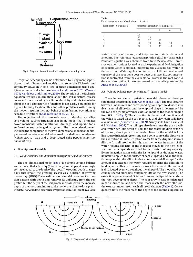

T. Sammis et al. / Agricultural Water Management 113 (2012) 30– 37 31

tcl1ecaats

stsip(a

2

2

wsddtpdi

Table 1Extraction percentage of water from ellipsoids.

Root depth (# of ellipsoid) Percentage extraction from ellipsoid

1 2 3 4 5

1 1002 72 28

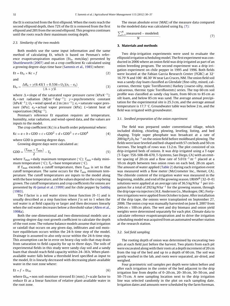
Fig. 1. Diagram of one-dimensional irrigation scheduling model.

Irrigation scheduling can be determined by using more sophis-icated multi-dimensional models that solve the Richard’s andontinuity equation in one, two or three dimensions using ana-ytical or numerical solutions (Warrick and Lomen, 1976; Warrick,974; Kandelous and Simunek, 2010). The solution of the Richard’squation requires information about the soil-moisture releaseurve and unsaturated hydraulic conductivity and this knowledgebout the soil characteristic functions is not easily obtainable for

given farming location. This and other problems with runninghe models result in their not being used in farming operations tochedule irrigations (Khodaverdiloo et al., 2011).

The objective of this research was to develop an ellip-oid volume-balance irrigation scheduling model that simulateswo-dimensional water infiltration, drainage, and uptake for aurface-line source-irrigation system. The model developmentncluded the comparison of the two-dimensional model to the sim-ler one-dimensional model when used in a shallow-rooted onionAllium cepa L.) crop and a deep-rooted chile pepper (Capsicumnnuum) crop.

. Description of models

.1. Volume balance one-dimensional irrigation scheduling model

The one-dimensional model (Fig. 1) is a simple volume-balanceater model that solves Eq. (1) on a daily time step and has a single

oil layer equal to the depth of the roots. The rooting depth changesaily throughout the growing season as a function of growingegree days (GDD). The one dimensional model has no root extrac-

ion pattern with depth and removes Et uniformly from the soilrofile, but the depth of the soil profile increases with the increaseepth of the root zone. Inputs to the model are climate data, plant-

ng data, harvest date, reference evapotranspiration, plant available

Fig. 2. Diagram of drip-irrigation sc

3 57 22 214 50 19 17 145 45 18 14 12 11

water capacity of the soil, and irrigation and rainfall dates andamounts. The reference evapotranspiration (Eto) for grass usingPenman’s equation was obtained from New Mexico State Univer-sity weather stations located at each experimental field. Irrigationor rainfall water is applied, increasing the available soil water inthe root zone. Water application in excess of the soil water-holdcapacity of the root zone goes to deep drainage. Evapotranspira-tion is subtracted from the available soil water in the root zone. Adetailed description of the one-dimensional model is presented byAndales et al. (2006).

2.2. Volume-balance two-dimensional irrigation model

The volume-balance drip-irrigation model is based on the ellip-soid model described by Ben-Asher et al. (1986). The row distancebetween line sources and corresponding soil depth are divided intofive halves of ellipsoids, and the ellipsoid shape is determined bythe ratio of x/y (major/minor axis), an input to the model rangingfrom 0.5 to 1 (Fig. 2). The x direction is the vertical direction, andthe value is based on the soil type. Clay and clay loam soils havea value of one (Ainechee et al., 2009). Sandy soils have a value of0.5 (Kirkham, 2005). The soil type also determines the plant avail-able water per unit depth of soil and the water holding capacityof the soil, also inputs to the model. Because the model is for aline source irrigation system and not a point source, the distance inthe z direction is unity. Irrigation water from the drip line sourcesfills the first ellipsoid uniformly, and then water in excess of thewater holding capacity of the ellipsoid moves to the next ellip-soid until all ellipsoids are filled to their water holding capacity.Excess irrigation water exits the last ellipsoid as drainage water.Rainfall is applied to the surface of each ellipsoid, and all the rain-fall stays within the ellipsoid that enters as rainfall except for theamount that exceeds the water required to bring the ellipsoid tofield capacity. This excess water moves to the next ellipsoid andis distributed evenly throughout the ellipsoid. The model has fiveequally spaced ellipsoids containing 20% of the row spacing. Theextraction percentage of Et taken from each ellipsoid depends on

the root development depth. The root growth rate is calculatedin the x direction, and when the roots reach the next ellipsoid,the extract amount from each ellipsoid changes (Table 1). Conse-quently, until the roots reach the depth of the second ellipsoid, all

heduling water-flow pattern.

3 ater M

tseu

2

meSa

E

a

E

wR(sv

hi

K

w

G

wm

cpwgp(

usw1

gootDTfelatw

E

wrt

2 T. Sammis et al. / Agricultural W

he Et is extracted from the first ellipsoid. When the roots reach theecond ellipsoid depth, then 72% of the Et is removed from the firstllipsoid and 28% from the second ellipsoid. This progress continuesntil the roots reach their maximum rooting depth.

.3. Similarity of the two models

Both models use the same input information and the sameethod of calculating Et, which is based on Penman’s refer-

nce evapotranspiration equation (Eto, mm/day) presented byhuttleworth (2007) and on a crop coefficient Kc calculated using

growing degree-days time base (Sammis et al., 1985) where:

t = Eto × Kc × f (2)

nd

to = �Rn + �(6.43(1 + 0.536 ∗ U2)(es − ea)(� + �)L

. (3)

here � = slope of the saturated vapor pressure curve (kPa K−1);n = net radiation (MJ m−2 day−1); � = psychrometric constantkPa K−1); U2 = wind speed at 2 m (m s−1); es = saturate vapor pres-ure (kPa); ea = actual vapor pressure (kPa); L = latent heat ofaporization (MJ kg−1).

Penman’s reference Et equation requires air temperature,umidity, solar radiation, and wind-speed data, and the values are

nputs to the model.The crop coefficient (Kc) is a fourth order polynomial where:

c = a + b ∗ GDD + c ∗ GDD2 + d ∗ GDD3 + e ∗ GDD4 (4)

here GDD is growing degree days.Growing-degree days were calculated as:

DD = (Tmax + Tmin)2

− Tb (5)

here Tmax = daily maximum temperature (◦C); Tmin = daily mini-um temperature (◦C); Tb = base temperature (◦C).If Tmax exceeds a cutoff temperature, then Tmax is set to that

utoff temperature. The same occurs for the Tmin minimum tem-erature. The cutoff temperatures are inputs to the model alongith the base temperature, and the values depend on the crop being

rown. The cutoff temperatures and crop coefficients for onions areresented by Al-Jamal et al. (1999) and for chile pepper by Saddiq1983).

The f factor is a soil water stress linear function (0–1) and issually described as a step function where f is set to 1 when theoil water is at field capacity or larger and then decreases linearlyhen the soil water decreases below a threshold value (Allen et al.,

998a).Both the one-dimensional and two-dimensional models use a

rowing-degree day root growth coefficient to calculate the depthf the root zone. The volume balance models assume that irrigationr rainfall that occurs on any given day, infiltrates and soil mois-ure equilibrium occurs within the 24-h time step of the model.rainage is assumed to also only occur within the 24-h time step.his assumption can be in error on heavy clay soils that may drainrom saturation to field capacity for up to three days. The soils ofxperimental fields in this study were sandy clay soil and a sandyoam that should reach field capacity within 24–36 h. When plant-vailable water falls below a threshold level specified as input tohe model, Et is linearly decreased with decreasing plant-availableater in the root zone where:

t = f × Etns (6)

here Etns = non soil-moisture stressed Et (mm); f = scale factor toeduce Et as a linear function of relative plant-available water inhe root zone.

anagement 113 (2012) 30– 37

The mean absolute error (MAE) of the measure data comparedto the modeled data was calculated using Eq. (7):∑N

i=1|measured − modeled|N

. (7)

3. Materials and methods

Two drip-irrigation experiments were used to evaluate theellipsoid irrigation scheduling model. The first experiment was con-ducted in 2006 where an onion field was drip irrigated as part of anonion breeding program. The second experiment was a drip irri-gation experiment on chile pepper in 1995 and 1996. Both fieldswere located at the Fabian Garcia Research Center (FGRC) at 32◦

16.79′ N and 106◦ 46.30′ W near Las Cruces, NM. The onion field soilwas a sandy clay loam classified as Glendale (fine-silty, mixed, cal-careous, thermic typic Torrifluvents) Harkey (coarse-silty, mixed,calcareous, thermic typic Torrifluvents) series. The top 60 cm soilprofile was classified as sandy clay loam, from 60 cm to 85 cm assilt loam, and below 85 cm was sand. The average annual precipi-tation for the experimental site is 25.3 cm, and the average annualtemperature is 17.7 ◦C. Groundwater table was below 2 m, and thefield was irrigated with groundwater.

3.1. Seedbed preparation of the onion experiment

The field was prepared under conventional tillage, whichincluded disking, chiseling, plowing, leveling, listing, and bedshaping. Triple super phosphate was broadcast at a rate of200 kg P2O5 ha−1 on the onion field before moldboard plowing. Thefields were laser leveled and bed-shaped with 57 cm beds and 50 cmfurrows. The length of rows was 13.2 m. The plot consisted of sixdrip-irrigated beds of onions. It was drip irrigated using a T-tape(T-Tape: TSX-508-08-670, T-Systems, San Diego, CA) with an emit-ter spacing of 20 cm and a flow rate of 5.0 l h−1 m−1 placed at a10 cm depth between two onion rows on each bed, 28 cm apart.The amount of water applied (Table 2) during each irrigation eventwas measured with a flow meter (McCrometer Inc., Hemet, CA).The chloride content of the irrigation water was measured in thebeginning, middle, and end of the growing season. URAN® (32–0–0)solutions were applied at an average rate of 36.5 kg N ha−1 per irri-gation for a total of 292 kg N ha−1 for the growing season, throughthe drip tape via injectors (H.E. Anderson Co., Muskogee, OK). Forty-two irrigations were applied from October to June. After installationof the drip tape, the onions were transplanted on September 27,2006. The onion crop was manually harvested on June 8, 2007 from244 cm × 100 cm plots. The wet and dry biomass and onion yieldweights were determined separately for each plot. Climate data tocalculate reference evapotranspiration and to drive the irrigationscheduling model was acquired from an automated weather stationat the research station.

3.2. Soil field sampling

The rooting depth of onion was determined by excavating twopits at each field just before the harvest. Two plants from each pitwere excavated along with their roots at a depth increment of 20 cmfrom the top of the bed and up to a depth of 60 cm. The soil wasgently washed in the lab, and roots were separated, air-dried, andweighed.

Four gravimetric soil samples per depth were taken before andafter each irrigation in the center of the bed adjacent to the drip

irrigation line from depths of 0–20 cm, 20–30 cm, 30–50 cm, and50–75 cm. A new sampling location next to the drip irrigationline was selected randomly in the plot on each sampling date.Irrigation dates and amounts were scheduled by the farm foreman.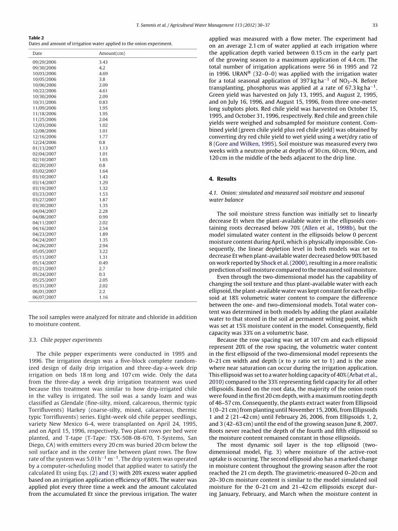

T. Sammis et al. / Agricultural Water M

Table 2Dates and amount of irrigation water applied to the onion experiment.

Date Amount(cm)

09/29/2006 3.4309/30/2006 4.210/03/2006 4.6910/05/2006 3.810/06/2006 2.0910/22/2006 4.6110/30/2006 2.0910/31/2006 0.8311/09/2006 1.9511/18/2006 1.9511/25/2006 2.0412/03/2006 1.0212/08/2006 1.0112/16/2006 1.7712/24/2006 0.801/13/2007 1.1302/04/2007 1.0102/10/2007 1.6502/20/2007 0.803/02/2007 1.6403/10/2007 1.4303/14/2007 1.2903/19/2007 1.3203/23/2007 1.5303/27/2007 1.8703/30/2007 1.3504/04/2007 2.2804/08/2007 0.9904/11/2007 2.0204/16/2007 2.5404/23/2007 1.8904/24/2007 1.3504/26/2007 2.9405/05/2007 3.2205/11/2007 1.3105/14/2007 0.4905/21/2007 2.705/24/2007 0.305/25/2007 2.0505/31/2007 2.02

Tt

3

1iifbicTtvapDsrbcbaf

06/01/2007 2.206/07/2007 1.16

he soil samples were analyzed for nitrate and chloride in additiono moisture content.

.3. Chile pepper experiments

The chile pepper experiments were conducted in 1995 and996. The irrigation design was a five-block complete random-

zed design of daily drip irrigation and three-day-a-week driprrigation on beds 18 m long and 107 cm wide. Only the datarom the three-day a week drip irrigation treatment was usedecause this treatment was similar to how drip-irrigated chile

n the valley is irrigated. The soil was a sandy loam and waslassified as Glendale (fine-silty, mixed, calcareous, thermic typicorrifluvents) Harkey (coarse-silty, mixed, calcareous, thermicypic Torrifluvents) series. Eight-week old chile pepper seedlings,ariety New Mexico 6-4, were transplanted on April 24, 1995,nd on April 15, 1996, respectively. Two plant rows per bed werelanted, and T-tape (T-Tape: TSX-508-08-670, T-Systems, Saniego, CA) with emitters every 20 cm was buried 20 cm below the

oil surface and in the center line between plant rows. The flowate of the system was 5.0 l h−1 m−1. The drip system was operatedy a computer-scheduling model that applied water to satisfy the

alculated Et using Eqs. (2) and (3) with 20% excess water appliedased on an irrigation application efficiency of 80%. The water waspplied plot every three time a week and the amount calculatedrom the accumulated Et since the previous irrigation. The water

anagement 113 (2012) 30– 37 33

applied was measured with a flow meter. The experiment hadon an average 2.1 cm of water applied at each irrigation wherethe application depth varied between 0.15 cm in the early partof the growing season to a maximum application of 4.4 cm. Thetotal number of irrigation applications were 56 in 1995 and 72in 1996. URAN® (32–0–0) was applied with the irrigation waterfor a total seasonal application of 397 kg ha−1 of NO3–N. Beforetransplanting, phosphorus was applied at a rate of 67.3 kg ha−1.Green yield was harvested on July 13, 1995, and August 2, 1995,and on July 16, 1996, and August 15, 1996, from three one-meterlong subplots plots. Red chile yield was harvested on October 15,1995, and October 31, 1996, respectively. Red chile and green chileyields were weighed and subsampled for moisture content. Com-bined yield (green chile yield plus red chile yield) was obtained byconverting dry red chile yield to wet yield using a wet/dry ratio of8 (Gore and Wilken, 1995). Soil moisture was measured every twoweeks with a neutron probe at depths of 30 cm, 60 cm, 90 cm, and120 cm in the middle of the beds adjacent to the drip line.

4. Results

4.1. Onion: simulated and measured soil moisture and seasonalwater balance

The soil moisture stress function was initially set to linearlydecrease Et when the plant-available water in the ellipsoids con-taining roots decreased below 70% (Allen et al., 1998b), but themodel simulated water content in the ellipsoids below 0 percentmoisture content during April, which is physically impossible. Con-sequently, the linear depletion level in both models was set todecrease Et when plant-available water decreased below 90% basedon work reported by Shock et al. (2000), resulting in a more realisticprediction of soil moisture compared to the measured soil moisture.

Even through the two-dimensional model has the capability ofchanging the soil texture and thus plant-available water with eachellipsoid, the plant-available water was kept constant for each ellip-soid at 18% volumetric water content to compare the differencebetween the one- and two-dimensional models. Total water con-tent was determined in both models by adding the plant availablewater to that stored in the soil at permanent wilting point, whichwas set at 15% moisture content in the model. Consequently, fieldcapacity was 33% on a volumetric base.

Because the row spacing was set at 107 cm and each ellipsoidrepresent 20% of the row spacing, the volumetric water contentin the first ellipsoid of the two-dimensional model represents the0–21 cm width and depth (x to y ratio set to 1) and is the zonewhere near saturation can occur during the irrigation application.This ellipsoid was set to a water holding capacity of 40% (Arbat et al.,2010) compared to the 33% representing field capacity for all otherellipsoids. Based on the root data, the majority of the onion rootswere found in the first 20 cm depth, with a maximum rooting depthof 46–57 cm. Consequently, the plants extract water from Ellipsoid1 (0–21 cm) from planting until November 15, 2006, from Ellipsoids1 and 2 (21–42 cm) until February 26, 2006, from Ellipsoids 1, 2,and 3 (42–63 cm) until the end of the growing season June 8, 2007.Roots never reached the depth of the fourth and fifth ellipsoid sothe moisture content remained constant in those ellipsoids.

The most dynamic soil layer is the top ellipsoid (two-dimensional model, Fig. 3) where moisture of the active-rootuptake is occurring. The second ellipsoid also has a marked changein moisture content throughout the growing season after the root

reached the 21 cm depth. The gravimetric-measured 0–20 cm and20–30 cm moisture content is similar to the model simulated soilmoisture for the 0–21 cm and 21–42 cm ellipsoids except dur-ing January, February, and March when the moisture content in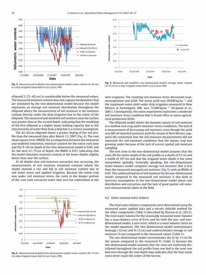

34 T. Sammis et al. / Agricultural Water Management 113 (2012) 30– 37

Fi

eTarecewoc

fimaaftb

mmswo

Fi

0

0.05

0.1

0.15

0.2

0.25

0.3

0.35

8/6/20074/28/20071/18/200710/10/20067/2/2006

Volu

met

ric

wat

er c

onte

nt

Date

Modeled

measured

ig. 3. Measured and modeled (two-dimensional model) water content (0–42 cm)n a drip-irrigated onion field in Las Cruces, NM.

llipsoid 2 (21–42 cm) is considerably below the measured values.he measured moisture content does not capture the dynamics thatre simulated by the two-dimensional model because the modelepresents an average soil moisture distribution throughout thellipsoid where the measurement of soil moisture is the moistureontent directly under the drip-irrigation line in the center of thellipsoid. The measured and modeled soil moisture near the surfaceas greater than at the second depth, indicating that the modeling

f the first ellipsoid at a higher water holding capacity due to theharacteristic of water flow from a drip line is a correct assumption.

The 42–63 cm ellipsoid shows a greater drying of the soil pro-le than the measured data after March 12, 2007 (Fig. 4). The rootean square error (RMSE) for a comparison between the measured

nd modeled volumetric moisture content for the entire root zonend the 0–20 cm depth of the two-dimensional model is 0.09, andor the next 21–75 cm of depth, the RMSE is 0.07, indicating thathe model simulates moisture content at the lower depths slightlyetter than near the surface.

At all depths that soil-moisture extraction was occurring, theeasurements of soil moisture remained constant where theodel showed a rise and fall in soil moisture content due to

oil water stress and applied irrigation. Because the onion cropas under soil moisture stress, the roots in the deeper portion

f the root zone extracted water that was not replenished at the

0

0.05

0.1

0.15

0.2

0.25

0.3

0.35

0.4

7/2/2006

Volu

met

ric

wat

erco

nten

t

10/10/2006 1/18/2007

Date

4/28/2007 8/6/20 07

ellipsoid 3 (ellipsoid 4 (30-50 cm m50-75 cm m

(42-63 cm)

(63-84cm )

measured

measured

ig. 4. Measured and modeled (two-dimensional model) water content (30–75 cm)n a drip-irrigated onion field in Las Cruces, NM.

Fig. 5. Measured and modeled (one-dimensional model) average water content(0–57 cm) in a drip-irrigated onion field in Las Cruces, NM.

next irrigation. The resulting soil moisture stress decreased evap-otranspiration and yield. The onion yield was 50,840 kg ha−1, andthe maximum onion yield under drip irrigation measured in NewMexico at Farmington, NM, was 73,000 kg ha−1 (Al-Jamal et al.,2001). Consequently, the onion experiment represents a moderatesoil moisture stress condition that is found often in onion agricul-tural production fields.

The ellipsoid model shows the dynamic nature of soil moisturein a shallow root crop under moisture-stress conditions. The lack ofa measurement of decreasing soil moisture, even though the yieldwas 68% of reported nonstress yield for onions in New Mexico, sup-ports the contention that the soil moisture measurements did notrepresent the soil moisture conditions that the onions crop wasgrowing under because of the lack of correct spatial soil moisturesampling.

The root zone in the one-dimensional model assumes that theroots fill the entire depth of the soil profile to a depth of 57 cm anda width of 107 cm and that the irrigated water depth is the sameeverywhere spatially. Generally speaking, the one-dimensionalwater-balance model computes average soil moisture that is lessthan the measured averaged soil moisture (Fig. 5) with an RMSE of0.05. This underestimation of soil moisture by the one-dimensionalmodel compared to the measured soil moisture is due both toincorrect assumptions in the one-dimensional model about rootdistribution and extraction and the lack of good spatial soil mois-ture measurements taken in the field.

4.2. Onion seasonal water balance

The total water balance components were determined using themeasured water applied data and a nitrate chloride method forthe other components (Table 3) described by Sharma et al. (2012).The total water balance for the seasonally measured water balancehas a mass balance error of 6 cm, and for both the one- and two-dimensional model, a zero error, which is a mass balance check onthe model equations. The two-dimensional model overestimatesdrainage (12 cm) and Et (3 cm) and underestimates storage in soilmoisture (4 cm) compared to the measured values (Table 3).

The one-dimensional model overestimates the Et by 11 cm forthe season compared to the measured Et (Table 3) because theone-dimensional model assumes that the roots are uniformly dis-

tributed throughout the soil profile from row bed to the next rowbed even through the root depth data indicates that the that onionroots never reach the center of the furrow.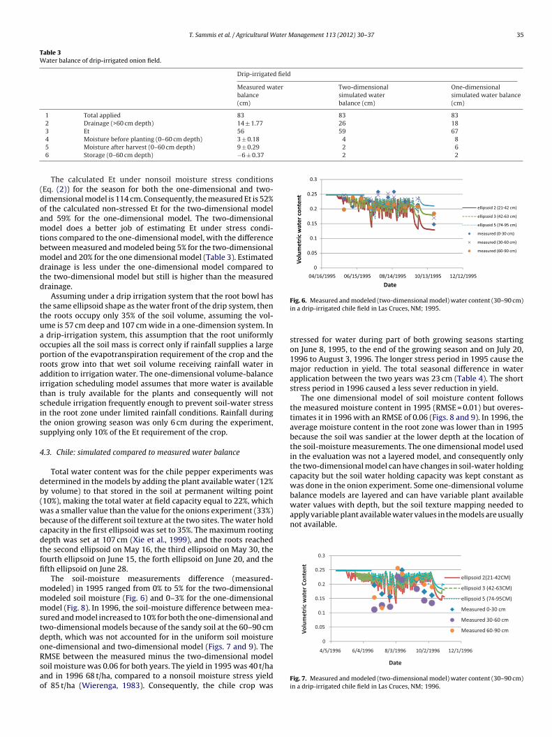

T. Sammis et al. / Agricultural Water Management 113 (2012) 30– 37 35

Table 3Water balance of drip-irrigated onion field.

Drip-irrigated field

Measured waterbalance(cm)

Two-dimensionalsimulated waterbalance (cm)

One-dimensionalsimulated water balance(cm)

1 Total applied 83 83 832 Drainage (>60 cm depth) 14 ± 1.77 26 183 Et 56 59 67

4 82 62 2

(doamtbmdtd

ttuaopraitsits

4

db(wbcdtffi

mmmstdoRsao

0

0.05

0.1

0.15

0.2

0.25

0.3

12/12/199510/13/199508/14/199506/15/199504/16/1995

Volu

met

ric

wat

erco

nten

t

Date

ellipsoi d 2 (21 -42 cm )

ellipsoi d 3 (42 -63 cm )

ellipsoi d 5 (74 -95 cm )

measured (0-30 cm )

measured (30 -60 cm )

measured (60 -90 cm )

apply variable plant available water values in the models are usuallynot available.

0

0.05

0.1

0.15

0.2

0.25

0.3

12/1/199610/2/19968/3/19966/4/19964/5/1996

Volu

met

ric

wat

er C

onte

nt

ellipsoi d 2(21-42CM )

ellipsoi d 3 (42-63CM )

ellipsoi d 5 (74-95CM )

Measured 0-30 cm

Measured 30-60 cm

Measured 60-90 cm

4 Moisture before planting (0–60 cm depth) 3 ± 0.18

5 Moisture after harvest (0–60 cm depth) 9 ± 0.29

6 Storage (0–60 cm depth) −6 ± 0.37

The calculated Et under nonsoil moisture stress conditionsEq. (2)) for the season for both the one-dimensional and two-imensional model is 114 cm. Consequently, the measured Et is 52%f the calculated non-stressed Et for the two-dimensional modelnd 59% for the one-dimensional model. The two-dimensionalodel does a better job of estimating Et under stress condi-

ions compared to the one-dimensional model, with the differenceetween measured and modeled being 5% for the two-dimensionalodel and 20% for the one dimensional model (Table 3). Estimated

rainage is less under the one-dimensional model compared tohe two-dimensional model but still is higher than the measuredrainage.

Assuming under a drip irrigation system that the root bowl hashe same ellipsoid shape as the water front of the drip system, thenhe roots occupy only 35% of the soil volume, assuming the vol-me is 57 cm deep and 107 cm wide in a one-dimension system. In

drip-irrigation system, this assumption that the root uniformlyccupies all the soil mass is correct only if rainfall supplies a largeortion of the evapotranspiration requirement of the crop and theoots grow into that wet soil volume receiving rainfall water inddition to irrigation water. The one-dimensional volume-balancerrigation scheduling model assumes that more water is availablehan is truly available for the plants and consequently will notchedule irrigation frequently enough to prevent soil-water stressn the root zone under limited rainfall conditions. Rainfall duringhe onion growing season was only 6 cm during the experiment,upplying only 10% of the Et requirement of the crop.

.3. Chile: simulated compared to measured water balance

Total water content was for the chile pepper experiments wasetermined in the models by adding the plant available water (12%y volume) to that stored in the soil at permanent wilting point10%), making the total water at field capacity equal to 22%, whichas a smaller value than the value for the onions experiment (33%)

ecause of the different soil texture at the two sites. The water holdapacity in the first ellipsoid was set to 35%. The maximum rootingepth was set at 107 cm (Xie et al., 1999), and the roots reachedhe second ellipsoid on May 16, the third ellipsoid on May 30, theourth ellipsoid on June 15, the forth ellipsoid on June 20, and thefth ellipsoid on June 28.

The soil-moisture measurements difference (measured-odeled) in 1995 ranged from 0% to 5% for the two-dimensionalodeled soil moisture (Fig. 6) and 0–3% for the one-dimensionalodel (Fig. 8). In 1996, the soil-moisture difference between mea-

ured and model increased to 10% for both the one-dimensional andwo-dimensional models because of the sandy soil at the 60–90 cmepth, which was not accounted for in the uniform soil moisturene-dimensional and two-dimensional model (Figs. 7 and 9). The

MSE between the measured minus the two-dimensional modeloil moisture was 0.06 for both years. The yield in 1995 was 40 t/hand in 1996 68 t/ha, compared to a nonsoil moisture stress yieldf 85 t/ha (Wierenga, 1983). Consequently, the chile crop was

Fig. 6. Measured and modeled (two-dimensional model) water content (30–90 cm)in a drip-irrigated chile field in Las Cruces, NM; 1995.

stressed for water during part of both growing seasons startingon June 8, 1995, to the end of the growing season and on July 20,1996 to August 3, 1996. The longer stress period in 1995 cause themajor reduction in yield. The total seasonal difference in waterapplication between the two years was 23 cm (Table 4). The shortstress period in 1996 caused a less sever reduction in yield.

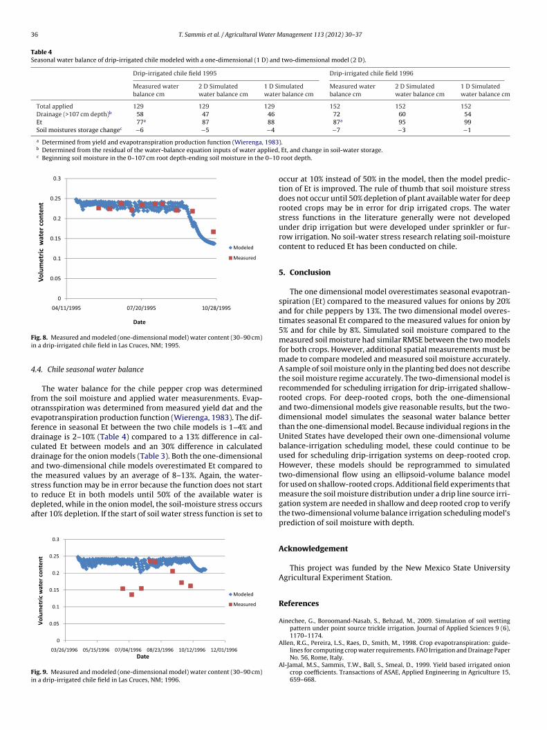
The one dimensional model of soil moisture content followsthe measured moisture content in 1995 (RMSE = 0.01) but overes-timates it in 1996 with an RMSE of 0.06 (Figs. 8 and 9). In 1996, theaverage moisture content in the root zone was lower than in 1995because the soil was sandier at the lower depth at the location ofthe soil-moisture measurements. The one dimensional model usedin the evaluation was not a layered model, and consequently onlythe two-dimensional model can have changes in soil-water holdingcapacity but the soil water holding capacity was kept constant aswas done in the onion experiment. Some one-dimensional volumebalance models are layered and can have variable plant availablewater values with depth, but the soil texture mapping needed to

Date

Fig. 7. Measured and modeled (two-dimensional model) water content (30–90 cm)in a drip-irrigated chile field in Las Cruces, NM; 1996.

36 T. Sammis et al. / Agricultural Water Management 113 (2012) 30– 37

Table 4Seasonal water balance of drip-irrigated chile modeled with a one-dimensional (1 D) and two-dimensional model (2 D).

Drip-irrigated chile field 1995 Drip-irrigated chile field 1996

Measured waterbalance cm

2 D Simulatedwater balance cm

1 D Simulatedwater balance cm

Measured waterbalance cm

2 D Simulatedwater balance cm

1 D Simulatedwater balance cm

Total applied 129 129 129 152 152 152Drainage (>107 cm depth)b 58 47 46 72 60 54Et 77a 87 88 87a 95 99Soil moistures storage changec −6 −5 −4 −7 −3 −1

a Determined from yield and evapotranspiration production function (Wierenga, 1983b Determined from the residual of the water-balance equation inputs of water applied,c Beginning soil moisture in the 0–107 cm root depth-ending soil moisture in the 0–10

0

0.05

0.1

0.15

0.2

0.25

0.3

10/28/199507/20/199504/11/1995

Volu

met

ric

wat

erco

nten

t

Date

Modeled

Measured

Fi

4

foefdcdatstda

Fi

ig. 8. Measured and modeled (one-dimensional model) water content (30–90 cm)n a drip-irrigated chile field in Las Cruces, NM; 1995.

.4. Chile seasonal water balance

The water balance for the chile pepper crop was determinedrom the soil moisture and applied water measurenments. Evap-transspiration was determined from measured yield dat and thevapotranspiration production function (Wierenga, 1983). The dif-erence in seasonal Et between the two chile models is 1–4% andrainage is 2–10% (Table 4) compared to a 13% difference in cal-ulated Et between models and an 30% difference in calculatedrainage for the onion models (Table 3). Both the one-dimensionalnd two-dimensional chile models overestimated Et compared tohe measured values by an average of 8–13%. Again, the water-tress function may be in error because the function does not start

o reduce Et in both models until 50% of the available water isepleted, while in the onion model, the soil-moisture stress occursfter 10% depletion. If the start of soil water stress function is set to

0

0.05

0.1

0.15

0.2

0.25

0.3

12/01/199610/12/199608/23/199607/04/199605/15/199603/26/1996

Vol

umet

ric

wat

er c

onte

nt

Date

Modeled

Measu red

ig. 9. Measured and modeled (one-dimensional model) water content (30–90 cm)n a drip-irrigated chile field in Las Cruces, NM; 1996.

). Et, and change in soil-water storage.

root depth.

occur at 10% instead of 50% in the model, then the model predic-tion of Et is improved. The rule of thumb that soil moisture stressdoes not occur until 50% depletion of plant available water for deeprooted crops may be in error for drip irrigated crops. The waterstress functions in the literature generally were not developedunder drip irrigation but were developed under sprinkler or fur-row irrigation. No soil-water stress research relating soil-moisturecontent to reduced Et has been conducted on chile.

5. Conclusion

The one dimensional model overestimates seasonal evapotran-spiration (Et) compared to the measured values for onions by 20%and for chile peppers by 13%. The two dimensional model overes-timates seasonal Et compared to the measured values for onion by5% and for chile by 8%. Simulated soil moisture compared to themeasured soil moisture had similar RMSE between the two modelsfor both crops. However, additional spatial measurements must bemade to compare modeled and measured soil moisture accurately.A sample of soil moisture only in the planting bed does not describethe soil moisture regime accurately. The two-dimensional model isrecommended for scheduling irrigation for drip-irrigated shallow-rooted crops. For deep-rooted crops, both the one-dimensionaland two-dimensional models give reasonable results, but the two-dimensional model simulates the seasonal water balance betterthan the one-dimensional model. Because individual regions in theUnited States have developed their own one-dimensional volumebalance-irrigation scheduling model, these could continue to beused for scheduling drip-irrigation systems on deep-rooted crop.However, these models should be reprogrammed to simulatedtwo-dimensional flow using an ellipsoid-volume balance modelfor used on shallow-rooted crops. Additional field experiments thatmeasure the soil moisture distribution under a drip line source irri-gation system are needed in shallow and deep rooted crop to verifythe two-dimensional volume balance irrigation scheduling model’sprediction of soil moisture with depth.

Acknowledgement

This project was funded by the New Mexico State UniversityAgricultural Experiment Station.

References

Ainechee, G., Boroomand-Nasab, S., Behzad, M., 2009. Simulation of soil wettingpattern under point source trickle irrigation. Journal of Applied Sciences 9 (6),1170–1174.

Allen, R.G., Pereira, L.S., Raes, D., Smith, M., 1998. Crop evapotranspiration: guide-

lines for computing crop water requirements. FAO Irrigation and Drainage PaperNo. 56, Rome, Italy.

Al-Jamal, M.S., Sammis, T.W., Ball, S., Smeal, D., 1999. Yield based irrigated onioncrop coefficients. Transactions of ASAE, Applied Engineering in Agriculture 15,659–668.

ater M

A

A

A

A

B

C

G

K

KK

K

T. Sammis et al. / Agricultural W

l-Jamal, M.S., Ball, S., Sammis, T.W., 2001. Comparison of sprinkler, drip and furrowirrigation efficiencies for onion production. Agricultural Water Management 46(3), 253–266.

llen, R., Pereira, L.S., Raes, D., Smith, M., 1998. Crop evapotranspiration – guidelinesfor computing crop water requirements. FAO Irrigation and Drainage, Paper 56.

ndales, A., Wang, J., Sammis, T.W., Mexal, J.G., Simmons, L.J., Miller, D.R., 2006.Pecan tree growth-irrigation-pruning management model. Agricultural WaterManagement 84 (1–2), 77–88.

rbat, G.P., Lamm, F.R., Abou Kheira, A.A., 2010. Subsurface drip irrigation emitterspacing effects on soil water redistribution, corn yield and water productivity.Transactions of the ASABE, Applied Engineering in Agriculture 26 (3), 391–399.

en-Asher, J., Charach, C.H., Zamel, A., 1986. Infiltration and water extraction fromdrip irrigation source: the effective hemispherical model. Soil Science Society ofAmerica Journal 50, 882–887.

ropWat, 2010. CropWat a crop water decision support tool. FAO version 8.http://www.fao.org/nr/water/infores databases cropwat.html.

ore, C.E., Wilken, W.W., 1995. New Mexico Agricultural Statistics. New MexicoAgricultural Statistical Service and United States Department of Agriculture, pp.69–70.

andelous, M.M., Simunek, J., 2010. Comparison of numerical, analytical and empir-ical models to estimate wetting patterns for surface and subsurface dripirrigation. Irrigation Science 29, L435–L444.

irkham, M.B., 2005. Principles of Soil and Plant Water Relations. Elsevier, p. 520.

hodaverdiloo, H., Homaee, M., van Genuchten, M.T., Dashtaki, S.G., 2011. Deriv-

ing and validating pedotransfer functions for some calcareous soils. Journal ofHydrology 399, 93–99.

S-State, 2010. KanSched – An ET Based Irrigation Scheduling Tool.,http://mobileirrigationlab.com/files/mil/KanSchedExcelUserGuide.pdf.

anagement 113 (2012) 30– 37 37

Michigan State University, 2010. Irrigation Scheduling Tools-irrigation, Fact Sheet3., http://www.ces.purdue.edu/ces/LaPorte/files/ANR/IrrFS3.pdf.

Saddiq, M.H., 1983. Soil Water Status and Water Use of Drip-Irrigated Chile PepperDissertation in Agronomy at NMSU.

Sammis, T.W., Mapel, C.L., Lugg, D.G., Lansford, R.R., McGuckin, J.T., 1985. Evapotran-spiration crop coefficients predicted using growing-degree-days? Transactionsof the ASAE 28 (3), 773–780.

Sharma, P., Shukla, M.K., Sammis, T.W., Steiner, R.L., John, G., Mexal, J.G., 2012.Nitrate–nitrogen leaching from three specialty crops of New Mexico under fur-row irrigation system. Agricultural Water Management 109, 71–80.

Shock, C.C., Feibert Erik, B.G., Saunders, L.D., 2000. Irrigation criteria for drip-irrigatedonions? Hortscience 35 (1), 63–66.

Shuttleworth, J., 2007. Putting the vap’ into evaporation? Hydrology and Earth Sys-tem Sciences 11 (1), 210–244.

Smith, M., Kivumbi, D., Heng, L.K., 2012. Use of the FAO CROPWAT Model in DeficitIrrigation Studies., http://www.fao.org/docrep/004/Y3655E/y3655e05.htm.

University of Arkansas, 2010. Computer Programs-Irrigation Scheduling Program.,http://www.aragriculture.org/computer programs/irrigation scheduling/default.asp.

Warrick, A.W., 1974. Time-dependent linearized infiltration. I. Point sources. SoilScience Society America Journal 38, 383L 386.

Warrick, A.W., Lomen, D.O., 1976. Time-dependent linearized infiltration. III. Stripand disc sources. Soil Science Society America Journal 40, 639L 643.

Wierenga, P. J. (1983). Yield and quality of drip-irrigated chile. NMSU AgricultureExperiment Station. Bulletin 703.

Xie, J., Cardenas, E.S., Sammis, T.W., Wall, M.M., Lindsey, D.L., Murray, L.W., 1999.Effects of irrigation method on chile pepper yield and phytophthora root rotincidence. Agriculture Water Management 42, 127L 142.