a two dimensional numerical soot model for advanced design
TRANSCRIPT

Graduate Theses, Dissertations, and Problem Reports
2011
A Two Dimensional Numerical Soot Model for Advanced Design A Two Dimensional Numerical Soot Model for Advanced Design
and Control of Diesel Particulate Filters and Control of Diesel Particulate Filters
Prabash E. Abeyratne West Virginia University
Follow this and additional works at: https://researchrepository.wvu.edu/etd
Recommended Citation Recommended Citation Abeyratne, Prabash E., "A Two Dimensional Numerical Soot Model for Advanced Design and Control of Diesel Particulate Filters" (2011). Graduate Theses, Dissertations, and Problem Reports. 4680. https://researchrepository.wvu.edu/etd/4680
This Thesis is protected by copyright and/or related rights. It has been brought to you by the The Research Repository @ WVU with permission from the rights-holder(s). You are free to use this Thesis in any way that is permitted by the copyright and related rights legislation that applies to your use. For other uses you must obtain permission from the rights-holder(s) directly, unless additional rights are indicated by a Creative Commons license in the record and/ or on the work itself. This Thesis has been accepted for inclusion in WVU Graduate Theses, Dissertations, and Problem Reports collection by an authorized administrator of The Research Repository @ WVU. For more information, please contact [email protected].
A Two Dimensional Numerical Soot Model
for Advanced Design and Control of Diesel
Particulate Filters
by
Prabash E. Abeyratne
Thesis submitted to theCollege of Engineering and Mineral Resources
at West Virginia Universityin partial fulfillment of the requirements
for the degree of
Master of Sciencein
Mechanical Engineering
Vincenzo Mulone, Ph.D.Gregory Thompson, Ph.D.
Victor Mucino, Ph.D.Mridul Gautam, Ph.D., Chair
Department of Mechanical and Aerospace Engineering
Morgantown, West Virginia2011
Keywords: Diesel Aftertreatment, Numerical Modeling, Emissions
Copyright 2011 Prabash E. Abeyratne

Abstract
A Two Dimensional Numerical Soot Model for Advanced Design and Control of DieselParticulate Filters
by
Prabash E. AbeyratneMaster of Science in Mechanical Engineering
West Virginia University
Mridul Gautam, Ph.D., Chair
One of the most effective methods to control diesel particulate matter (PM) emissions from heavy dutydiesel engines is to use wall flow diesel particulate filters (DPF). It is still a major challenge to get anaccurate estimation of soot loading, which is crucial for the engine afterteratment assembly optimization.In the recent past, several advanced computational models of DPF filtration and regeneration have beenpresented to assess the cost effective optimization of future particulate trap systems. They are characterizedby different degree of detail and computational costs, depending on the specific application (i.e diagnostics,control, system design, component design etc)
The objective of this study is to compare in detail a two dimensional (2-D) approach with a one dimen-sional (1-D) approach, thus giving a better insight of the variation of properties over the DPF length. Thistask has been archived by extending an in-house developed 1-D numerical soot model to the next dimensionto understand the impact of 2-D representation to predict both steady state and transient behavior of a cat-alyzed diesel particulate filter (CDPF). Performance of the model was evaluated using three key parameters:pressure drop, filter outlet temperature and soot mass retained in the filter during both active and continuousregeneration events. Quasi-steady state conservation of mass, momentum and energy equations were solvednumerically using finite difference methods adopting a spatially uniform mesh. The results obtained fromthe current model were compared with the 1-D code to evaluate the general validity of assumptions madein the latter, especially DPF loading status prediction.
The model was validated using the data gathered at the West Virginia University Engine and EmissionsResearch Laboratory (WVU-EERL) using a model year 2004 Mack MP7-355E Diesel engine coupled to aJohnson Matthey catalyzed diesel particulate filter (CDPF) exercised over a 13 mode European stationarycycle (ESC) followed by two federal transient cycles (FTP). A constant set of model tuning parameters weremaintained for the sake of general validation of simplifying assumptions of the 1-D code.
The analysis shows that the predicted pressure drop across the DPF is in good agreement with the dataobtained at EERL in both steady state and transient cycles. It is also shown that the soot accumulatesmainly in the frontal and rear parts across the filter length under given soot concentrations. The model iscapable of tracking DPF soot mass satisfactorily with a maximum discrepancy of 3.47g during steady statecycle. A 7.95% decrease in soot layer thickness can be seen in the front portion of the DPF during thetransient cycle mainly due to O2 assisted regeneration at elevated temperatures. Both 1-D and 2-D modelsproduce similar results during the loading phase. However, the current model is able to capture regenerationphase of the FTP cycle more descriptively than the 1-D model. The discrepancy of the reported totalsoot mass estimation between two models was 2.12%. The distribution corresponding to the 1-D model isrepresentative of soot layer distribution given by the 2-D model at one tenth distance away from the DPFfront face. 1-D model representation is effective towards PM prediction, although presenting considerableaxial effects at higher DPF temperatures.

iii
Acknowledgements
As my graduate studies come to an end, many people come to my mind that I am grateful
for. First, my deepest appreciation goes to my beloved family. Ammi, I will never be able
to thank you enough for the strength and support you have given me for all my life. You are
my inspiration and I’m forever in your debt for the sacrifices you have made during my road
to success. Aiyya, the love and support you gave was the strength for me to stand even in
difficult times in my life.
I would like to thank my academic advisor Dr. Mridul Gautam for his constant support
and encouragement. His support has been invaluable to my education, academic progress and
professional development. I extend my sincere thanks to Dr. Vincenzo Mulone for providing
me valuable and thought-provoking ideas throughout my research. I would also like to thank
other members of my committee Dr. Gergory Thompson and Dr. Victor Mucino for their
support and valuable recommendations to my thesis.
I would like to extend my gratitude to my colleagues Alessandro Cozzolini, Daniele Littera,
Clay Bell, Mario Velardi and Gennaro Campitelli for providing such a friendly and dynamic
atmosphere in the office. I enjoyed working with you all and thank you for lending me a
helping hand whenever I wanted.
Finally I would like to express my heartiest thanks to all my Sri Lankan friends Oshadha,
Kaushi, Thilanka, Bhakthi, Nipuni, Saman aiyya, Sumudu aiyya and Yudheesha nangi for
being such great friends and leaving numerous happy memories in the past six years of my
life.

iv
Contents
Acknowledgements iii
List of Figures vi
List of Tables viii
Notation ix
1 Introduction 1
2 Literature Review 52.1 Emission Regulations . . . . . . . . . . . . . . . . . . . . . . . . . . . . . . . 52.2 Emission Formation in Diesel Engine . . . . . . . . . . . . . . . . . . . . . . 6
2.2.1 Hydrocarbons (HC) . . . . . . . . . . . . . . . . . . . . . . . . . . . . 62.2.2 Carbon Monoxide (CO) . . . . . . . . . . . . . . . . . . . . . . . . . 72.2.3 Oxides of Nitrogen (NOx) . . . . . . . . . . . . . . . . . . . . . . . . 72.2.4 Particulate matter (PM) . . . . . . . . . . . . . . . . . . . . . . . . . 8
2.3 Diesel Emission Control Technologies . . . . . . . . . . . . . . . . . . . . . . 92.3.1 In-cylinder Control Strategies . . . . . . . . . . . . . . . . . . . . . . 92.3.2 Diesel Exhaust Aftertreatment Devices . . . . . . . . . . . . . . . . . 11
2.4 Numerical Modeling . . . . . . . . . . . . . . . . . . . . . . . . . . . . . . . 23
3 Model Description 263.1 Model Overview . . . . . . . . . . . . . . . . . . . . . . . . . . . . . . . . . . 263.2 Wall Filtration Model . . . . . . . . . . . . . . . . . . . . . . . . . . . . . . . 283.3 Regeneration Model . . . . . . . . . . . . . . . . . . . . . . . . . . . . . . . . 35
3.3.1 Cake Regeneration Submodel . . . . . . . . . . . . . . . . . . . . . . 353.3.2 Washcoat Regeneration Submodel . . . . . . . . . . . . . . . . . . . . 403.3.3 Wall Regeneration Submodel . . . . . . . . . . . . . . . . . . . . . . . 423.3.4 Wall Energy Balance . . . . . . . . . . . . . . . . . . . . . . . . . . . 433.3.5 Mass, Momentum and Energy Balance . . . . . . . . . . . . . . . . . 46
4 Numercal Procedure 504.1 Solving the Boundary Value Problem . . . . . . . . . . . . . . . . . . . . . . 504.2 Solving the Initial Value Problem . . . . . . . . . . . . . . . . . . . . . . . . 52

CONTENTS v
5 Experimental Setup and Procedures 565.1 Instrumentation and Laboratory Setup . . . . . . . . . . . . . . . . . . . . . 565.2 Experimental Procedure . . . . . . . . . . . . . . . . . . . . . . . . . . . . . 58
6 Results and Discussion 616.1 Steady State Cycle Analysis . . . . . . . . . . . . . . . . . . . . . . . . . . . 626.2 Transient Cycle Analysis . . . . . . . . . . . . . . . . . . . . . . . . . . . . . 706.3 1-D and 2-D Model Comparison . . . . . . . . . . . . . . . . . . . . . . . . . 74
6.3.1 Steady State Cycle Results Comparison . . . . . . . . . . . . . . . . . 746.3.2 Transient Cycle Results Comparison . . . . . . . . . . . . . . . . . . 77
7 Conclusions 81
A Model Validation Using Bissett Model 83
References 85

vi
List of Figures
2.1 High pressure loop EGR (left) and low pressure loop EGR (right) [17] . . . . 102.2 Diesel oxidation catalyst (DOC) [18] . . . . . . . . . . . . . . . . . . . . . . 112.3 Selective catalytic reduction system [20] . . . . . . . . . . . . . . . . . . . . 132.4 Fuel burner for DPF regeneration [16] . . . . . . . . . . . . . . . . . . . . . . 172.5 Burner by-pass system for light duty application [16] . . . . . . . . . . . . . 182.6 Electrically regenerated DPF [24] . . . . . . . . . . . . . . . . . . . . . . . . 192.7 Catalyzed continuously regenerating technology (CCRT) [25] . . . . . . . . . 21
3.1 Schematic of a single channel of the diesel particulate filter . . . . . . . . . . 263.2 Model block diagram . . . . . . . . . . . . . . . . . . . . . . . . . . . . . . . 283.3 Unit collector loading . . . . . . . . . . . . . . . . . . . . . . . . . . . . . . . 293.4 Schematic of the particle deposition on filter channels . . . . . . . . . . . . 353.5 Sectional view of DPF with thermal resistance parameters . . . . . . . . . . 45
5.1 FTP reference data, exhaust flow rate, exhaust gas specie concentrations andCPF inlet temperature [40] . . . . . . . . . . . . . . . . . . . . . . . . . . . . 59
6.1 Experimental pressure drop of the DPF during the loading cycle . . . . . . . 636.2 Experimental and simulated pressure drop profiles pertaining to four loading
cycles . . . . . . . . . . . . . . . . . . . . . . . . . . . . . . . . . . . . . . . 646.3 Experimental and simulated DPF outlet temperature of the 8th loading cycle 656.4 Experimental and simulated DPF outlet temperature of the 8th loading cycle 666.5 Model predicted filter pressure drop during 18-22 hour time duration during
the loading phase . . . . . . . . . . . . . . . . . . . . . . . . . . . . . . . . . 676.6 Soot layer thickness evolution with time along channel length during a loading
cycle . . . . . . . . . . . . . . . . . . . . . . . . . . . . . . . . . . . . . . . . 686.7 Soot layer thickness evolution with time along channel length during a loading
cycle . . . . . . . . . . . . . . . . . . . . . . . . . . . . . . . . . . . . . . . . 686.8 Soot layer thickness evolution with time along channel length during a loading
cycle . . . . . . . . . . . . . . . . . . . . . . . . . . . . . . . . . . . . . . . . 696.9 Experimental and simulated DPF soot mass comparison during the loading
phase . . . . . . . . . . . . . . . . . . . . . . . . . . . . . . . . . . . . . . . . 706.10 Pressure drop comparison between experimental and numerical data over an
FTP cycle . . . . . . . . . . . . . . . . . . . . . . . . . . . . . . . . . . . . . 716.11 Experimental vs. simulated DPF pressure drop . . . . . . . . . . . . . . . . 71

LIST OF FIGURES vii
6.12 Mass balance of DPF during the FTP cycle . . . . . . . . . . . . . . . . . . 726.13 Soot layer thickness distribution along normalized CPF channel length (above);
Temporal decay of soot layer thickness at different axial locations (below) . . 736.14 Wall velocity distribution comparison along filter length . . . . . . . . . . . . 756.15 1-D and 2-D DPF soot mass prediction comparison . . . . . . . . . . . . . . 766.16 Total soot mass predictions of 1-D and 2-D models . . . . . . . . . . . . . . 786.17 Temperature distribution variation at different axial locations . . . . . . . . 786.18 DPF outlet temperature prediction comparison . . . . . . . . . . . . . . . . 796.19 Soot layer thickness prediction of 1-D and 2-D models . . . . . . . . . . . . . 80
A.1 DPF pressure drop validation using Bissett model . . . . . . . . . . . . . . . 83A.2 Mass retained in the DPF validation using Bissett model . . . . . . . . . . . 84

viii
List of Tables
2.1 Heavy-duty compression-ignition engines and urban buses exhaust emissionstandards [13] . . . . . . . . . . . . . . . . . . . . . . . . . . . . . . . . . . . 6
4.1 Grid resolution comparison . . . . . . . . . . . . . . . . . . . . . . . . . . . . 50
5.1 Test engine manufacturer specifications . . . . . . . . . . . . . . . . . . . . . 575.2 Geometrical dimensions of the DOC/DPF . . . . . . . . . . . . . . . . . . . 575.3 Test point data . . . . . . . . . . . . . . . . . . . . . . . . . . . . . . . . . . 585.4 Exhaust gas emissions before DOC and after DPF for soot loading mode, 1800
rpm, 10% load [40] . . . . . . . . . . . . . . . . . . . . . . . . . . . . . . . . 605.5 Exhaust gas emissions before DOC and after DPF for soot regeneration mode,
1800 rpm, 100% load [40] . . . . . . . . . . . . . . . . . . . . . . . . . . . . . 605.6 The average engine out brake specific emissions during two FTP cycles . . . 60
6.1 Model tuning parameters and constants . . . . . . . . . . . . . . . . . . . . . 626.2 Coefficient of determination comparison relevent to 1-D and 2-D model pre-
dicted and experimental pressure drop during the 30 hour loading phase . . . 746.3 Coefficient of determination comparison relevent to 1-D and 2-D model pre-
dicted and experimental pressure drop during transient cycles . . . . . . . . 77

ix
Notation
Symbols
A : pre-exponential factor in Arrhenius equation, [m/s/K0.21]Asoot : area of soot particles, [m2]b : unit spherical cell size, [m]C : PM mass concentration, [kg/m3
cpg : gas phase heat capacity, [J/kg/K]cpp : particulate layer heat capacity, [J/kg/K]cps : substrate heat capacity, [J/kg/K]D : hydraulic diameter, [m]dc : unit collector diameter, [m]dc0 : inital unit collector diameterDpore : pore diamter, [m]E : activation energy, [J/kmol]Ecake : cake filtration efficiency [-]F : friction coefficient, [-]fCO : thermal selectivity, [-]g(ε) : Kuwabara hydrodynamic factor, [-]gCO : CO selectivity of soot oxidation by NO2
Hex : convective heat transfer coefficient of the DPF, [J/m2/s/K]∆H : heat of reaction, [J/kmol]hi : convective heat transfer coefficient of channel i, [J/m2/s/K]kcat : rate of catalytic doot oxidation, [m/s]kp : particulate layer permeability, [m2]kth : rate coefficient of thermal soot oxidation, [m/s]L : DPF length, [m]MC : molecular weight of carbon, [kg/kmol]Mi : molecular weight of ith exhaust gas specie, [kg/kmol]Pe : Peclet number, [-]Pi : pressure in ith channel, [Pa]Qw : volumetric flow rate, [m3/s]R : universal gas constant, [J/kmol/K]Ra : Rayleigh number, [-]

x
Ri,j : ith specie consumption rate in the jth layer, [kmol/m2/s]Rt : thermal resistance, [sK/J]R : radius, [m]Sp : specific soot area of deposit layer, [1/m]Ti : temperature of ith channel, [K]T : time, [s]vi : gas velocity in the ith channel, [m/s]ws : substrate wall thickness, [m]w : particulate layer thickness, [m]x : transverse direction (distance through the wall), [m]Y : mass fraction, [-]y : mole fraction, [-]z : axial direction, [m]
Greek symbols
α : thermal diffusivity, [m2/s]β : index of completeness of soot oxidation, [-]βth : thermal expansion coefficient, [1/K]λ : thermal conductivity, [J/msK]ν : kinematic viscosity, [m2/s]ε : porosity, [-]η : efficiency, [-]ρi : gas density in ith channel, [kg/m3]ρsoot,ck : soot packing density, [kg/m3]µ : dynamic viscosity, [kg/m/s]ψ : percolation factor, [-]φ : partition coefficient, [-]
Abbrevitions
CDPF : Catalyzed Diesel Particulate FilterC : CarbonCO : Carbon MonoxideCO2 : Carbon DioxideCVS : Constant Volume SamplingDOC : Diesel Oxidation CatalystDPF : Diesel Particulate FilterECU : Electronic Control Unit

xi
EEPS : Engine Exhaust Particle SizerEERL : Engine and Emissions Research LaboratoryEGR : Exhaust Gas RecirculationESC : European Stationary CycleExhAUST : Exhaust Aftertreatment Unified Simulation ToolNOx : Oxides of NitrogenO2 : OxygenPM : Particulate MatterUSLD : Ultra Low Sulfer Diesel FuelVGT : Variable Geometry Turbocharger
Subscripts
1 : inlet channel2 : outlet channelatm : atmosphericcat : catalyticcond : conductioneng : engineenvir : environmenti : gas specieins : insulationp : particulate layerreact : reactions : substrateth : thermalwall : wall

1
Chapter 1
Introduction
Diesel engines have been traditionally identified in the US as the best solution for heavy
duty transportation and off road applications in general terms of cost and reliability. Im-
proved fuel economy and attainment of high torque at lower speeds have recently attracted
the attention of the passenger vehicle market in the US for diesel engines, while their market
share in Europe is already well established. Exhaust emissions and diesel engines comprise
of a wide range of compounds. But the regulated emissions include hydrocarbons (HC),
carbon monoxide (CO), oxides of nitrogen (NOx) and particulate matter (PM).
Diesel particulate filter (DPF) has earned its reputation as one of the highly effective
methods to control PM emissions from diesel engines. The most commonly used DPF design
is the wall flow monolith. In this design, adjacent channels are alternatively plugged at each
end in order to force the diesel soot particles to flow through the substrate wall. Thus,
diesel PM is deposited on the sides of the inlet channel. The deposited PM affects the
flow and temperature field inside the trap, and increases the pressure drop across the trap.
An excessive back pressure will raise the fuel penalty and potentially damage the engine.
A regeneration process is therefore required to remove the deposited PM from the DPF.
This can be performed either continuously with the use of catalyst (passive regeneration) or
periodically via hydrocarbon combustion, electric heating [1] and microwave heating [2, 3].

CHAPTER 1. INTRODUCTION 2
However, the optimization of DPF performance metrics whilst maintaining optimal fuel ef-
ficiency depends on extensive laboratory and on-road testing. Diesel engines operate through
a wide range of operating conditions. Steady state operating conditions vary greatly from
the transient operating conditions. Engine speed, torque, power output and exhaust tem-
perature at a given engine operation condition differ and significantly impact the exhaust
composition.
The application of simulation tools provides a promising alternative to traditional design
of experiments approach; thereby minimizing the complex and expensive engine testing
resources. These models are capable of providing insight in to local parameters such as
temperature, velocity, density and pressure drop parameters opposed to spatially averaged
values obtained through experiments. Thorough knowledge of each of these parameters is
crucial to optimization of next generation DPF systems.
Several numerical models have been developed to globally simulate the soot loading ca-
pacity, the pressure drop evolution and regeneration behavior of wall flow filters [4, 5, 6].
These range from zero to three dimensional models. One dimensional (1-D) models are
computationally efficient and can be used to get a quick estimation of the pressure drop
and regeneration characteristics of the DPF. Konstandopoulos et al.[7] showed an excellent
agreement between 1-D and 3-D model predictions over a variety of filter media. How-
ever, 1-D models assume constant properties along the channel length. Properties such as,
soot layer thickness, wall temperature and wall velocity do vary under real world situations.
There is a possibility of having local hot spots in certain parts of the monolith wall, which
may not be tracked by a 1-D model, since it only provides an averaged value in the axial
direction. In practice, a controlled and predictable reaction is required, considering that
these filters should last through a large number of regeneration cycles. Multi scale analytical
models help understanding the details of the complex processes and improving the filters
and the regeneration processes. Two dimensional models facilitate tracking the aforemen-
tioned parameters, at the expense of an additional computational effort. Three dimensional
(3-D) models provide the most accurate descriptions of the DPF filtration and regeneration

CHAPTER 1. INTRODUCTION 3
parameters. However, these models are usually quite intensive in computational effort and
time. Thus, 2-D models provide the means to obtain reasonable accuracy and predictability
without being computationally intensive.
The primary objective of the thesis is to develop a two dimensional numerical soot model
for a DPF to analyze the impact of close-to-real descriptions of filtration, regeneration process
and heat transfer. The secondary objective of the thesis is to validate the developed model
using both steady state and transient driving cycles. Federal test procedure (FTP) cycle is
more realistic, though not exact simulation; of actual driving conditions than a steady state
cycle. The author finds the numerical studies carried out in this area to be quite limited
[8, 9, 10].
The developed model uses a finite difference scheme to solve mass, momentum and en-
ergy equations. A lumped model was used to simulate the filtration process to make the
code computationally efficient. Both catalytic and thermal assisted soot oxidation processes
were implemented to capture regeneration behavior of modern catalyzed diesel particulate
filters (CDPF). The results of the simulations include the prediction of development of tem-
perature, pressure, channel velocity and soot layer thickness along the filter length. The
developed model may be utilized as a tool to design a DPF’s geometrical, physical and
chemical parameters in order to optimize its performance for a given test configuration.
Differentiating from the study of transient operating conditions simulated using a smooth
sinusoidal function by Rumminger [8] and Khan [9], results of the current study are based on
Federal Test Procedure (FTP) cycle. During a typical driving cycle, the DPF is subjected to
highly transient conditions, thus generating varying exhaust mass and volumetric flow rates,
gas composition, temperature, PM content and particle size distribution. The experimental
data to support validation of the DPF model was gathered at West Virginia University
Engine Emissions and Research Laboratory (EERL). The model was successfully able to
capture the pressure drop and temperature characteristics of the DPF during transient engine
operation.
4
Chapter 2
Literature Review
2.1 Emission Regulations
Owing to health and environmental concerns arise from various engine emissions, the
Environmental Protection Agency (EPA) in the United States established regulations under
the clean air act amendments (CAAA). The four main emission species HC, CO, NOx and
PM, were considered as the main pollutants in both the US and European union (EU).
Exposure to high levels of CO concentrations could lead to fatigue and chest pain for people
with a history of heart disease [13]. Oxides of nitrogen are highly reactive gases and play a
pivotal role in the formation of ozone, smog and acid rain [13]. Diesel fuel combustion has
shown to produce the largest amount of particulate matter (PM) mass compared to gasoline
and alternative fuels, which has been identified as a potential occupational carcinogen by
the National Institute for Occupational Safety and Health (NIOSH) [15].
Table 2.1 shows that from 1998 to 2007, the emission limits for NOx and PM have been
tightened by 95% and 90% respectively for heavy-duty compression-ignition engines. The
control of emissions has thus become one of the most prominent areas of diesel engine re-
search.

CHAPTER 2. LITERATURE REVIEW 5
Table 2.1: Heavy-duty compression-ignition engines and urban buses exhaust emission stan-dards [13]
Year HC NMHC NOx NMHC+NOx PM CO
(g/bhp-hr) (g/bhp-hr) (g/bhp-hr) (g/bhp-hr) (g/bhp-hr) (g/bhp-hr)
1974-78 - - - 16 - 401979-84 1.5 - - 10 - 251985-87 1.3 - 10.7 - - 15.51988-89 1.3 - 10.7 - 0.6 15.5
1990 1.3 - 6 - 0.6 15.51991-93 1.3 - 5 - 0.25 15.51994-97 1.3 - 5 - 0.1 15.5
1998-2003 1.3 - 4 - 0.1 15.52004-2006 - - - 2.4 0.1 15.5
2007 - 0.14 0.2 2.4 0.01 15.5
2.2 Emission Formation in Diesel Engine
2.2.1 Hydrocarbons (HC)
In a diesel engine, fuel resides in the combustion chamber for a shorter time than in spark
ignition engine. Hence the likelihood of unburned HC formation is much less in a diesel
engine in comparison to the other. Three main mechanisms of HC emission formation in
a diesel engine are (1) extremely lean mixtures; (2) extremely rich mixtures; and (3) flame
quenching and misfire.
In an event where fuel is injected during an ignition delay, the mixtures obtained are too
lean because the fuel is partially consumed in the thermal oxidation later in the expansion
phase after mixing with additional air. The amount of unburned hydrocarbons originating
in these lean areas depends on the quantity injected during the ignition delay, the mixing
rate with air during this period and auto-ignition conditions prevailing in the cylinder.
The main cause of HC formation in rich mixtures is the nozzle sac volume. Nozzle sac is
a hollow circular cavity located at the tip of the needle downstream of its seat. At the end

CHAPTER 2. LITERATURE REVIEW 6
of the injection event, the injector sac volume remains full of fuel. During the combustion
and expansion phases, this fuel partially vaporizes and penetrates into the cylinder at low
speeds. This fuel slowly mixes with air and bypasses the main combustion process. Hence, at
minimum ignition delay for direct ignition engine, the HC emissions are directly proportional
to the nozzle sac volume [11]. Moreover, in transient operations such as acceleration, there
is a possibility of excessive injection of fuel into the combustion chamber. This may cause
high local fuel/air ratios during expansion and exhaust phases.
Flame quenching at the walls is another source of HC emissions. Ignition deficiencies
which give rise to high HC emissions typically occur at low compression rates and abnormally
delayed injection. These ignition events occur during cold starts and can be visually identified
from the formation of white smoke, a mist of microdroplets of unburned fuel.
2.2.2 Carbon Monoxide (CO)
Carbon monoxide is formed mainly due to incomplete combustion due to lack of O2 and
is a function of temperature and residence time. Combustion of fuel rich mixtures usually
produces high CO emissions. Since diesel engines always operate on an overall lean mixture,
CO emissions are typically lower than that of gasoline engines.
2.2.3 Oxides of Nitrogen (NOx)
Nitric oxide (NO) and nitrogen dioxide (NO2) are collectively identified as oxides of ni-
trogen (NOx), where NO accounts for the larger portion of the two. The main source of NO
formation is diatomic nitrogen (N2), which covers the most significant portion of atmospheric
air per volume basis. NO2 is formed by recombination reactions between NO and various
other oxidants. NO2 emission can only be seen prominent at engine temperatures below
1200K. At higher temperatures it will quickly revert back to NO in the presence of O2.
Extended Zeldovitch mechanism has been widely accepted as the principal cause of NOx
formation. These reactions typically occur at temperature well above 2000K. Three main
chemical reactions that contribute to this mechanism can be described as follows.

CHAPTER 2. LITERATURE REVIEW 7
O2 + 2N2 → 2NO + 2N (2.1)
N +O2 → NO +O (2.2)
N +OH → NO +H (2.3)
NO emissions produced due to this mechanism appear in significant quantities well after
start of heat release phase since the aforementioned reactions are relatively slow and very
sensitive to temperature. High fuel/air ratios favor NOx formation as more fuel is burned;
more heat is produced with an increase in combustion temperature. Higher nozzle open-
ing pressures also promote NOx formation due to improved combustion efficiency with the
presence of smaller fuel particles. Retarding injection timing has a desirable effect on NO
formation as it is related to the premixed portion of the fuel. Fuel cetane number, swirl and
intake charge dilution also contributes to NOx formation [12].
2.2.4 Particulate matter (PM)
Particulate matter is defined as all substances which under normal circumstances are
present in exhaust gases in a solid (ash, carbon) or liquid state [13]. PM is generated due to
incomplete combustion of diesel fuel. When diesel fuel is sprayed into the cylinder at high
pressure, the sprayed fuel droplets do not mix completely with the abundant oxygen at a
molecular level. This results in incomplete combustion. Dust or inorganic material in the
fuel or fuel additives also contributes to diesel PM in the form of ash. Presence of sulfur in
the fuel and lubrication oil contributes to sulfate formation. This material is referred to as
the soluble organic fraction (SOF).
In the burning of liquid fuels of the diesel type, the size of the droplet is extremely
important because the formation of soot increases with size. The non-homogeneous nature
of the mixture, duration of the injection and its overlap with combustion are parameters that
CHAPTER 2. LITERATURE REVIEW 8
influence the process of soot formation. The list below summarizes the main parameters that
influence diesel particulate formation [16].
(1) Formation of insoluble fraction: elevated temperature, high pressure and absence of
oxygen.
(2) Formation of organic compounds of particles: lean mixture zones, temperature below
the flammability limit, HC layers on the walls of the cylinder, fuel droplets dribbling at the
nozzle tip.
(3) Sources of particles from lubricant: surface of cylinder liners, valve stem gaskets, turbo-
stem gaskets and recycling of crankcase ventilation gases into inlet.
2.3 Diesel Emission Control Technologies
2.3.1 In-cylinder Control Strategies
Exhaust gas recirculation (EGR) is considered as one of the most efficient methods to
reduce NOx emissions from diesel engines. The basic EGR operation is to re-circulate a
portion of the exhaust gas back to the intake manifold. When exhaust gas is introduced into
the combustion chamber and mixed with dilution air, total heat capacity of the mixture gets
elevated. Reduction of peak combustion temperature assists abatement of NOx formation.
However, net thermal efficiency of the engine reduces due to reduction in peak combustion
temperature. Consequently, the fuel consumption and the PM emissions of the engine may
increase. This is the major drawback of this technology.
EGR was first introduced in 1970s and today most diesel engines use in its standard
configuration [17]. If the exhaust gas is recycled to the intake manifold directly, the operation
is called hot EGR. If the exhaust gas is routed via an EGR cooler, the operation is called cold
EGR. Implementation of EGR for a turbocharged engine is somewhat difficult in comparison
to a naturally aspirated engine. There are two common EGR configurations for turbocharged
engines; (1) low pressure loop EGR and (2) high pressure loop EGR (see Figure 2.1). Low
pressure loop EGR depends on the differential pressure created between turbine outlet and
compressor inlet. Partial throttling also helps to increase the tailpipe pressure to drive the

CHAPTER 2. LITERATURE REVIEW 9
flow. However, high pressure loop EGR is the most common implementation method. In
this configuration, exhaust gas is re-circulated from upstream of the turbine to downstream
of compressor. This differential pressure may be controlled using intake throttling, exhaust
restriction and venture device. However, this configuration leads to an increase in fuel
consumption and PM emissions.
Figure 2.1: High pressure loop EGR (left) and low pressure loop EGR (right) [17]
Multiple fuel injection (MFI) strategy also helps to reduce NOx and PM emissions. The
idea behind this strategy is to reduce the peak combustion temperature in cylinder by spread-
ing the fuel to be burned over a relatively longer period of time. Moreover, MFI strategy can
be combined with a high pressure fuel injection system to enhance fuel atomization. This
helps in archiving lower PM emissions. However, simultaneous reduction of both engine-out
NOx and PM emissions can be limited by the NOx/PM tradeoff.
Low temperature combustion (LTC) and premixed combustion are also promising tech-
nologies for simultaneous reduction of both NOx and PM emissions. As discussed earlier,

CHAPTER 2. LITERATURE REVIEW 10
lowering combustion temperature helps in reducing NOx emissions whilst premixing helps
to reduce PM emissions. Low temperature combustion is achieved using increased levels
of EGR to reduce the oxygen concentration present in the combustion chamber. Premixed
combustion is accomplished by prolonging the ignition delay and dispersion of the injected
fuel.
2.3.2 Diesel Exhaust Aftertreatment Devices
Diesel Oxidation Catalyst (DOC)
A DOC can be used across a range of exhaust temperatures and is an efficient method of
reducing HC and CO in low exhaust temperature applications. The substrate is typically of
honeycomb construction and each channel surface consists of a precious metal coating such
as rhodium and vanadium.
Figure 2.2: Diesel oxidation catalyst (DOC) [18]
DOCs are typically used to reduce the SOF component of the particulate matter as shown
in the following equation.
SOF +O2 → CO2 +H2O (2.4)
DOCs can also be used to effectively reduce the amount of HC and CO emissions. Major
reactions in a DOC is given in equations (2.5)-(2.7).
CHAPTER 2. LITERATURE REVIEW 11
CO +1
2O2 → CO2 (2.5)
C3H6 +9
2O2 → 3CO2 + 3H2O (2.6)
C3H8 + 5O2 → 3CO2 + 4H2O (2.7)
Typically SOF, HC and CO oxidation reactions take place in very high temperature condi-
tions. However, the use of catalysts allows these reactions to take place at significantly lower
temperatures. The reduction of CO emissions is almost entirely accomplished by noble met-
als, whereas HC conversion is attributed to both washcoat and noble metal loading. When
the DOC reaches a certain temperature the oxidation reactions take place almost immedi-
ately. This temperature is called the “light-off temperature.”Above this point, conversion
efficiencies rapidly reach steady state. Extensive research efforts continues to this date, to
reduce the light off temperature aiming to increase DOC performance during cold starts.
However, the catalytic performance of the DOC will gradually worsen throughout its
lifetime. This is called the “Aging effect.”Typical diesel fuel consists of minute percentage
of sulfur at the parts per million level. Sulfates formed at high temperatures contribute to
total particulates and deactivation of the catalyst through its interaction with sulfuric acid
(see equations (2.8) and (2.9)). The aging process can be retarded to a certain extent with
the use of ultra low sulfur diesel (ULSD).
SO2 +1
2O2 → SO3 (2.8)
SO3 +H2O → H2SO4 (2.9)
Exposure to high operating temperatures leads to catalyst thermal destruction, a process
known as “sintering”that causes DOC efficiency to plunge due to scarcity of precious metal
surface area.

CHAPTER 2. LITERATURE REVIEW 12
Selective Catalytic Reduction
Selective catalytic reduction (SCR) is a proven catalyst technology capable of reducing
NOx emissions to meet stringent EPA 2010 standards. Basic components of a SCR system
is shown in Figure 2.3.
Figure 2.3: Selective catalytic reduction system [20]
SCR uses catalyst and ammonia to convert NOx into H2O and N2 using the following
hydrolysis reactions.
4NO + 4NH3 +O2 → 4N2 + 6H2O
NO + 2NH3 +O2 +NO2 → 2N2 + 3H2O
2NO2 + 4NH3 +O2 → 3N2 + 6H2O
(2.10)
The catalytic layer of the SCR consists of three main catalysts: TiO2, V2O5 and WO3.
Vanadia (V2O5) is the main contributor of the NOx abatement. However, it also promotes
oxidation of sulfer and create sulfuric acid which poisons the very catalyst. Tungsten oxide
(WO3) widens the temperature window of the SCR reactions which helps improving the
mechanical and structural properties of the catalyst [19].
The urea solution used for the SCR system is a mixture of 32.5% urea and 67.5% water.
When urea is injected in to exhaust stream, it decomposes and creates ammonia. The SCR

CHAPTER 2. LITERATURE REVIEW 13
process requires precise control of urea injection rates. Insufficient injection amounts will
result in unacceptably low NOx reduction and excessive injection will result in ammonia
slip. SCR can operate over a large temperature range (200-600◦C) [21]. However, SCR is a
complex system and requires sophisticated control systems. Diesel engines typically operate
in highly transient conditions. Thus the control system should constantly adjust the amount
of urea injected in to the catalyst in order to reduce ammonia slip. Catalyst deactivation
due to sulfur poisoning and thermal deactivation due to sintering could also hurt the SCR
performance.
Diesel Particulate Filter
Perhaps most effective approach in combating PM is the DPF, which are more colloquially
known as PM traps. The DPFs can be classified under two main categories depending on
the respective operating principal:
(1) Deep bed filters; and
(2) Shallow bed filters.
Deep bed filters collect or trap particles throughout the whole filter (3-D), whilst shallow bed
filters only accumulate soot on the wall (2-D). However, deep bed filtration can be regarded
as the more generalized case since the pore diameters of most common filter materials (≥
1µm) are often much larger than typical particle sizes present in diesel exhaust.
The selection of DPF materials are not based on their filtration properties, but more on
their thermal and mechanical properties. Filter wall should withstand high temperatures
that occur due to high exothermic reactions. Cordierite is the most commonly used DPF
material [5]. This synthetic ceramic material (2MgO.2Al2O3.5SiO2) has been initially devel-
oped for automotive catalytic converters. Low thermal expansion coefficient of this material
resists extreme thermal cycling and high temperature gradients, increasing the mechanical
integrity of the filter. Silicon carbide (SiC) is another popular choice and has a better ther-
mal resistivity than Cordierite. Higher thermal expansion coefficient of this material gives
arise to a packaging issue. SiC is also more expensive than Cordierite. Ceramic DPFs are
also available and is usually combined with one or more material. Ceramic DPFs provide

CHAPTER 2. LITERATURE REVIEW 14
greater leeway in channel geometry and better assist with filter design, geometry and shape.
Metal fiber particulate traps show their advantages in electrically assisted regeneration pro-
cess. Filter wall cracking due to high local temperature gradients can be avoided owing to
its better thermal conductivity. However, metal DPFs are usually more expensive than the
other materials discussed in this section.
The filtration mechanism in a DPF depends on filter material and design. The most
commonly used filter design is the wall flow monolith. In this design, adjacent channels are
alternatively plugged at each end in order to force the diesel soot particles to flow through
the substrate wall. Thus, diesel PM is deposited on the sides of the inlet channel. Filter
walls have a porous structure that is carefully controlled during the manufacturing process.
Typical values of material porosity are between 45 and 50% whilst the pore size varies from
10 to 20µm.
Deep bed filtration relies mainly on three mechanism of aerosol deposition [33]:
(1) Brownian diffusion;
(2) Inertial impaction; and
(3) Interception collection.
As the name suggest, Brownian diffusion depends on the Brownian movement exhibited by
small particulates, particularly below 0.3 µm in diameter.
The trajectories of these small particles do not correspond to those of the streamlines but
rather diffuse from the gas to the surface of the monolith wall. Large particles suspend in
the exhaust flow tend to stick in to an oncoming obstruction due to their inertial effects.
This is known as the inertial impaction. The intensity of this mechanism increases with
increasing particle size and flow velocity. Small, less dense particles which travel along flow
streamline and flow close to the filter wall contributes to soot layer deposition without being
influenced by inertia or Brownian diffusion. This mechanism is known as the interception
collection. Other collection mechanism like gravitational settling, inertial deposition and
thermophoresis are known to be insignificant given the conditions and particle sizes of diesel

CHAPTER 2. LITERATURE REVIEW 15
exhaust [33].
The deposited PM affects the flow and temperature field inside the trap, and increases
the pressure drop across the trap. An excessive back pressure will raise the fuel penalty
and potentially damage the engine. A regeneration process is therefore required to remove
the deposited PM from the DPF by oxidizing soot particles. Soot oxidation reactions re-
quire exhaust temperatures well above 500◦C with available oxygen concentration and flow
velocities. Typical diesel engines do not produce exhaust temperatures in this magnitude.
Hence, numerous regeneration techniques have been suggested over the last two decades.
These can be categorized into two principal methods: (1) active regeneration and (2) passive
regeneration.
Active regeneration systems trigger regeneration by raising the temperature suitable for
soot oxidation with the use of an external energy source. The regeneration of the filter has
to be manually initiated at pre-determined intervals. Usually it is based on the distance
travelled. The three most widely used energy sources are: (1) diesel fuel combustion, (2)
electrical heating and (3) microwave heating.
Diesel fuel combustion is the preferred and most commonly used method of all. It is
readily available in a vehicle and is about five times energy efficient than the other active
regeneration methods [22]. A proper fuel combustion based regeneration strategy is evaluated
upon several guidelines [23]: (1) maximum temperature increase at minimum fuel expense;
(2) minimum noise pollution; (3) minimum byproduct formation due to the regeneration
event and (4) minimum dependency on the driver.
This is achieved by several ways. One method is to heat up the exhaust gas by a throttling
event. Soot oxidation initiate when exhaust gas reach the desired temperature. However,
this is not the most efficient method in this regard as the engine power is decreased during
throttling. It also reduces the remaining oxygen content making the regeneration control
difficult. However, it helps increasing the filter life as lower oxygen concentrations lead to
lower filter wall temperatures due to the reduced exotherm.

CHAPTER 2. LITERATURE REVIEW 16
Another method is to place a diesel fueled burner in front of the DPF (see Figure 2.4) .
This method is capable of carrying out the regeneration process at all engine speed and load
conditions. The regeneration process is initiated when the back pressure across the filter
reaches a specified level. Sudden and significant increase in DPF outlet temperature is also
a good indicator of the onset of the regeneration. However, such a system requires proper
control of the sophisticated electronics and a large air pump to heat up the entire exhaust
gas to 540◦C. High pressure burner fuel system is also required to maintain the filter inlet
temperature to a desired level. Also the system should ensure continuous air circulation
through the burner nozzle to minimize fouling effects by particle deposits.
Figure 2.4: Fuel burner for DPF regeneration [16]
Newer systems overcome many of the above issues by using a bypass system, isolating the
filter from the engine exhaust during the regeneration process. A schematic of such a system
is given in Figure 2.5. This method requires nearly an order of magnitude less energy to
heat up the filter face entirely [23]. This configuration also requires a smaller blower to route
exhaust gas through the system and less complicated electronic control system for its proper
operation.

CHAPTER 2. LITERATURE REVIEW 17
Figure 2.5: Burner by-pass system for light duty application [16]
Electrical Regeneration
Electrically assisted regeneration is also a popular choice amongst DOF regeneration
techniques. The main advantage of this method is the absence of the fuel economic penalty.
The necessary electrical demand is provided by the vehicle battery or off board the vehicle
using an electrical outlet. During on-road regeneration, an increase in the idle speed to avoid
unacceptable levels of battery discharge. The method also lets the trap to be regenerated at
all speed and load conditions.
Electrical heating can be applied in a number of configurations, such as placing an elec-
trical heater upstream of DPF (see Figure 2.6) or heating the entire DPF enclosing body.
Typical heaters are fabricated from two nichrome resistance elements contained in MgO
power insulation. A small air pump is used to transfer the heat from heater to the filter.
Heating is discontinued when the trap inlet temperature reach 760◦C [16].

CHAPTER 2. LITERATURE REVIEW 18
Figure 2.6: Electrically regenerated DPF [24]
Incorporating electrical heating elements in to the filter structure is another common way
of employing electrically assisted filter regeneration. In this way, the soot could be ignited
directly without the necessity of heating all the exhaust gas. RYPOS and MAN+HUMMEL
are current manufacturers of such systems.
Aerodynamic Regeneration
Aerodynamic regeneration or compressed air regeneration method removes PM trap in-
side the DPF by emitting a sequence of compressed air pulses through its channels, in a
direction opposite to that of the exhaust flow. The compressed air required for this opera-
tion is readily available from the compressor system used for braking. However, the system is
capable of regenerating the trap even when the vehicle is in motion since the interruption to
the flow is momentary. During a thermal regeneration phase, incombustible materials such
as ash remain and accumulate in the filter wall over time. This leads to an irreversible plug-
ging effect of the DPF, limiting the filter in-use service life. The compressed air pulses used
in this method further helps flushing out this residual ash content. Moreover, the method
averts complex sensing and control issues pertaining to the techniques described earlier in
this section.

CHAPTER 2. LITERATURE REVIEW 19
Microwave Regeneration
Garner and Dent reported regeneration efficiencies of 40-80% with microwave regener-
ation. Microwave heating is accomplished by a method similar to electrical heating. In
this method, soot is heated directly by the microwaves while the filter wall is heated only
by conduction and convection, or in other words, no exothermic reactions occur on the fil-
ter wall. Hence, microwave regenerated DPFs have improved resistance to melting during
regeneration.
Plasma Regeneration
Oxygen could be activated by applying non-thermal plasma to generate ozone, which
could then be used to combust soot at low temperatures. However, this approach has not
been used in commercial applications yet.
The main advantage of active regeneration is that the onset of regeneration is guaranteed
regardless of the operating conditions. However, it has to embrace a significant fuel economy
penalty in achieving it. Fuel needed for the burner, fuel consumed in driving the alternator
for electrical heating, the energy needed for ancillary equipment such as blowers, installation
of complicated systems and effectiveness of the heat energy transferred to the PM are just
to name a few. Also care must be taken to limit the filter temperature to about 1400◦C to
prevent melting or cracking of the filter.
In passively regenerating DPF systems the soot oxidation happens during the normal
operation of the vehicle without any action required by either the operator or the engine
control system. Passive regeneration systems usually use catalyst to lower the temperature at
which soot oxidizes to the temperature of exhaust stream. There are mainly two approaches
for passive regeneration: (1) using a combination of DOC and DPF and (2) fuel additives.
Good catalytic reaction requires a greater catalytic surface area. To increase the surface
area for a good distribution of the precious metal catalyst material so-called washcoat layer
is used. The main function of the washcoat layer is to stabilize the fine dispersed catalyst
material against sintering, but can also be used to enhance the catalytic activity or protect

CHAPTER 2. LITERATURE REVIEW 20
it against poisoning. The typical range for washcoat loading is between 3 and 300 g/dm3
catalyst volume with typical metal loadings of 0.110 g/dm3 catalyst [16]. Washcoat is con-
sisted of noble metals such as platinum, palladium and rhodium. Rhodium and vanadium
also help suppress the catalytic oxidation of SO2 which increases the life of the catalyst.
There are number of different washcoat based passive regeneration systems available in
todays market. Continuously regenerating trap (CRT) system contains a DOC upstream of
a DPF. Catalyzed soot filter (CSF) uses a catalytic coating placed inside the DPF to carry
out the passive regeneration activity. The most commonly used method is the Catalyzed
continuously regenerating technology (CCRT) developed by Johnson Matthey and is shown
in Figure 2.7. This system contains a DOC upstream of the CSF which allows maximum
use of NOx for soot regeneration.
Figure 2.7: Catalyzed continuously regenerating technology (CCRT) [25]
A CSF system is more compact than a CRT system as it requires only one component
instead of two. But its compactness requires compromises regarding exhaust backpressure
and catalyst loading. The soot layer on top of the filter walls burns less effectively in a CSF
than a CRT system. This is because in a CSF NO is oxidized to NO2 underneath the soot

CHAPTER 2. LITERATURE REVIEW 21
layer whereas in a CRT system NO2 is formed upstream of the DPF and has therefore a
higher chance to contact the soot layer on top of the filter walls.
A CSF system requires less installation space but higher operating temperatures than a
CRT system. In a CSF, NOx can potentially be used more than once for soot oxidation. At
high enough temperatures the NOx to PM ratio requirements can be lower for CSFs than for
CRT systems. However, due to its design a CRT system is less sensitive to ash accumulation
and more robust against sintering of the precious metal components. Ash accumulation in
CSF reduces efficiency due to blocking of gas pathways as the ash plug builds up. Precious
metal sintering is a high temperature ageing mechanism leading to a reduced number of
catalytically active sites.
In case of spontaneous thermal regenerations with oxygen the carbon burning creates heat
within the DPF. Such heat would not affect an upstream DOC, like in the CRT setup, but
the catalytic coating of the CSF would be fully exposed to it. If the temperature on the
CSF surface becomes too high, this could potentially cause some precious metal sintering
resulting in catalyst deactivation. Both systems have advantages and disadvantages. Thus,
the choice of system depends on the application.
The CCRT system benefits advantages of both CRT and CSF systems. It allows a more
efficient use of the NOx emitted from the engine for carbon burning. This is especially true
for low temperature applications and applications with a low NOx to PM ratio.
The second approach is the use of catalyst in the form of liquid fuel additives. This liquid
solution contains oxides of base metals such as barium, calcium, cerium, cobalt, chromium,
lanthanum, manganese, and vanadium. In this way, the catalyst enters the engine combustion
chamber with the fuel and the soot particles formed during the combustion phase contain
the catalyst. Soot particles are hence able to oxidize at low temperatures.
One of the main drawbacks of these systems is the lack of pure contact between the
catalytic coating and the soot particles. The particles that are in direct contact with the

CHAPTER 2. LITERATURE REVIEW 22
catalytic layer are only able to oxidize. Catalytic layer poisoning due to oxidation of SO2
is another drawback. When SO2 gets mixed with water, it produces sulfuric acid which
immensely reduces the filter life through poisoning.
2.4 Numerical Modeling
As discussed in the previous chapter, in order to minimize the complex and expensive
engine testing resources, a number of computational models have been presented thus far in
literature, elaborating on DPFs functionality. These models are characterized by different
degrees of detail in particulate transport along the channel length. Significant progress
towards understanding the complicated transport and regeneration processes was gained by
the pioneering work of Bissett [4, 26] who provided a mathematical model for the analysis
of regeneration in DPF. This was a zeroth dimensional (0-D) model which performed well in
cases where DPF is subjected to large flow rates. Bissett later developed a more general single
layer one dimensional model to capture filtration/regeneration characteristics at sufficiently
low engine speeds [27]. This model considered the conservation of mass, momentum and
energy inside filters including soot oxidation reactions.
Konstandopoulos and Johnson [28] derived a one-dimensional analytical solution for the
flow field and pressure drop of a clean DPF based on Bissetts model. With the assumption
that the porous wall was a collection of spherical collectors, they employed diffusion and
interception mechanisms to describe clean DPF filtration characteristics.
A two-layer model was later developed by Konstandopoulos and Kostoglou [29] to account
for the effects of incomplete contact between the particulate layer and catalyst coated on the
porous wall. Different soot oxidation rates for thermal and catalytic layers were employed
in this model by evaluating oxygen depletion rates. Mass and momentum balance equations
were solved using a Runge-Kutta Nystrom method opposed to the Glarkin finite element
method used in Bissett model. With this approach, Konstandopoulos was able to develop a
better numerical model in terms of computational efficiency.

CHAPTER 2. LITERATURE REVIEW 23
Haralampous and Koltsakis [30, 31] studied the oxygen diffusion and NO2 back-diffusion on
DPF regeneration. The role of oxygen diffusion was shown to be important in uncontrolled
regenerations, which could cause high peak temperature. The contribution of NO2 back
diffusion was responsible for about one third of the total regeneration rate for CDPFs. The
significance of NO2 assisted soot oxidation at lower monolith wall temperatures was discussed
in a previous study [32] of the same institute.
Opris and Johnson developed [33, 34] a two-dimensional computational model to study
the flow, heat transfer and regeneration behaviors of DPF. The inclusion of the viscous dissi-
pation term is significant in this model. This study also discussed the filtration mechanisms
of the monolith wall in detail. The inertial and interception effects showed greater filtration
efficiencies when particle diameters become larger. The opposite effect happens when parti-
cle diameters become smaller. In this case, it was found that Brownian diffusion contributes
towards better filtration efficiency. Zhang et al. [35] also presented a two-dimensional single-
channel model to simulate filter performance. An analytical approximation for the flow field
was developed by simplifying the Navier-Stokes equations through an order of magnitude
analysis approach. Then the flow field was employed to solve for the temperature field
followed by species concentration balance.
Koltsakis et al. [10] developed a one-dimensional mathematical model to predict tempera-
ture gradient inside particulate layer and porous wall in the flow direction through the wall.
It was found that significant temperature gradient existed under some operating conditions,
which were associated with high flow rate and large initial particulate loading. Kladopoulou
et al. [36] developed a lumped parameter model to describe the performance of particulate
filter. This model assumed that the temperature of the particulate filter did not have spatial
variation and was considered to be uniform over the whole control volume.
Konstandopoulos et al. [37] also developed a 3-D DPF model using commercially available
computational fluid dynamics (CFD) software and compared its results with a 1-D model.
The author demonstrated excellent agreement between analytical solutions of 1-D single

CHAPTER 2. LITERATURE REVIEW 24
channel model and 3-D CFD results.
Schejbal et al. [38] studied the ash deposition on the inlet channel of the DPF in an aged
filter. The results of this study revealed that the differences between the fresh and aged
filters towards filtration/regeneration characteristics to be quite small.
Recently, a model discussing advanced filtration and regeneration process treatment to
the wall was presented by Mulone et. al [39] and allowed to analyze the evolution of soot
layer thickness in detail. Conventionally, the soot oxidation was analyzed by descritizing
the soot layer in to several parts. A 1-D fully analytical treatment was novel and unique
characteristic of this model and allowed to represent with great detail key phenomena for
DPF modeling, without any discretization error.
A majority of the models described so far in this section were tested and validated when
the engine is operating in steady state conditions. The transient DPF model developed
by Rumminger et al. [8] concluded that time varying temperature input to a soot loaded
filter could cause faster regeneration with the assistance of faster reaction rates. He further
identified cell density and the type of catalytic coating as parameters which could also
contribute to this effect. Khan et al. [9] validated their model under transient conditions
simulated using a sinusoidal modulation in the exhaust temperature and mass flow rate of the
filter inlet. It was found that the modulated temperature could increase the life of the filter as
it promotes low temperature regeneration process. However, these temperature fluctuations
may not be easily produced by an engine in its actual driving conditions. Kandylas et
al. [10] validated their model using a European Transient driving Cycle (ETC) which was
representative of real road driving. The model was able to successfully predict the operation
of a CRT system.

25
Chapter 3
Model Description
3.1 Model Overview
Mathematical model presented in this chapter for DPF pressure drop and regeneration is
based mainly on the works by Bissett [4] and Kostandopoulos[5]. The model assumes that
the exhaust gas entering into any given inlet channel presents identical but time dependent
mass flow velocities irrespective of its radial position. However, in reality, the channels closer
to the walls may show different thermodynamic and fluid dynamic properties. Since, the
model in the present study focused on two dimensional behavior of the DPF, aforementioned
assumption is justified. This assumption leads authors to describe characteristics of all DPF
channels by evaluating just one channel (unit channel approach).
Figure 3.1: Schematic of a single channel of the diesel particulate filter

CHAPTER 3. MODEL DESCRIPTION 26
A schematic of a single channel in the DPF is given in Figure 3.1. Axial distance along
the channel is denoted by the z coordinate and the transverse direction (distance through
the wall) is denoted by the x direction.
Exhaust gas temperatures, densities, velocities and pressures are treated as cross-sectional
averaged values. All these values depend only on time t and z direction. The oxygen mass
fraction is a function of all three dimensions (x,z and t) due to exothermic soot oxidation in
the wall. The pressure difference across the channel cross section is assumed to be negligible.
Hence the mass transfer in the z direction between neighboring cells and the wall is also
considered to be negligible. Previous work has shown [4] that heat conduction between
substrate wall and diesel particulates to be so dominant that the particulate temperature is
treated the same as the substrate wall. This assumption allows treatment of the soot particle
temperature only as a function of z and t. Heat loss of the exhaust gas along the channel
length is considered to be governed by the convection heat transfer rather than conduction
heat transfer due to high Peclet numbers. Exhaust gas density was expressed in terms of
temperature via the ideal gas law. The effect of ash loading in the DPF wall on the pressure
drop is also considered to be negligible.
In general, the developed model is capable of simulating the DPF behavior for a variety
of engine cycles. The main structure of the model is illustrated in Figure 3.2. First, the
code reads the input file and defines simulation conditions such as DPF geometrical charac-
teristics, exhaust gas property definitions, initial / boundary conditions and reaction kinetic
parameters. The model then calculates the flow field and the energy balance equations along
the inlet and outlet channels. Based upon these properties the model calculates soot layer
evolution in the substrate wall using the filtration model and the regeneration model. The
regeneration model consists of three submodels, namely cake, washcoat and wall submod-
els. Finally, the substrate layer energy balance is solved and results are assigned as initial
conditions for the next iteration.

CHAPTER 3. MODEL DESCRIPTION 27
Figure 3.2: Model block diagram
3.2 Wall Filtration Model
The filtration model under investigation is based on the framework developed by Konstan-
dopoulos et al. [5, 7]. Recently Mulone et al. [39] extended this work further by developing
a fully analytical wall filtration model opposed to classical wall representation by slabs. The
analytical approach presented in [39] was developed further by Cozzolini et al. [40] where
layer collection mechanism and wall filtration have been linked together taking into account
CHAPTER 3. MODEL DESCRIPTION 28
the soot layer thickness, similarly to what was presented by Mohammed et al. [6].
Models with such higher degree of detail level show greater complexities which in turn
necessitate a greater demand in computational power. The current study uses a computa-
tionally efficient 0-D filtration model to avert such complexities.
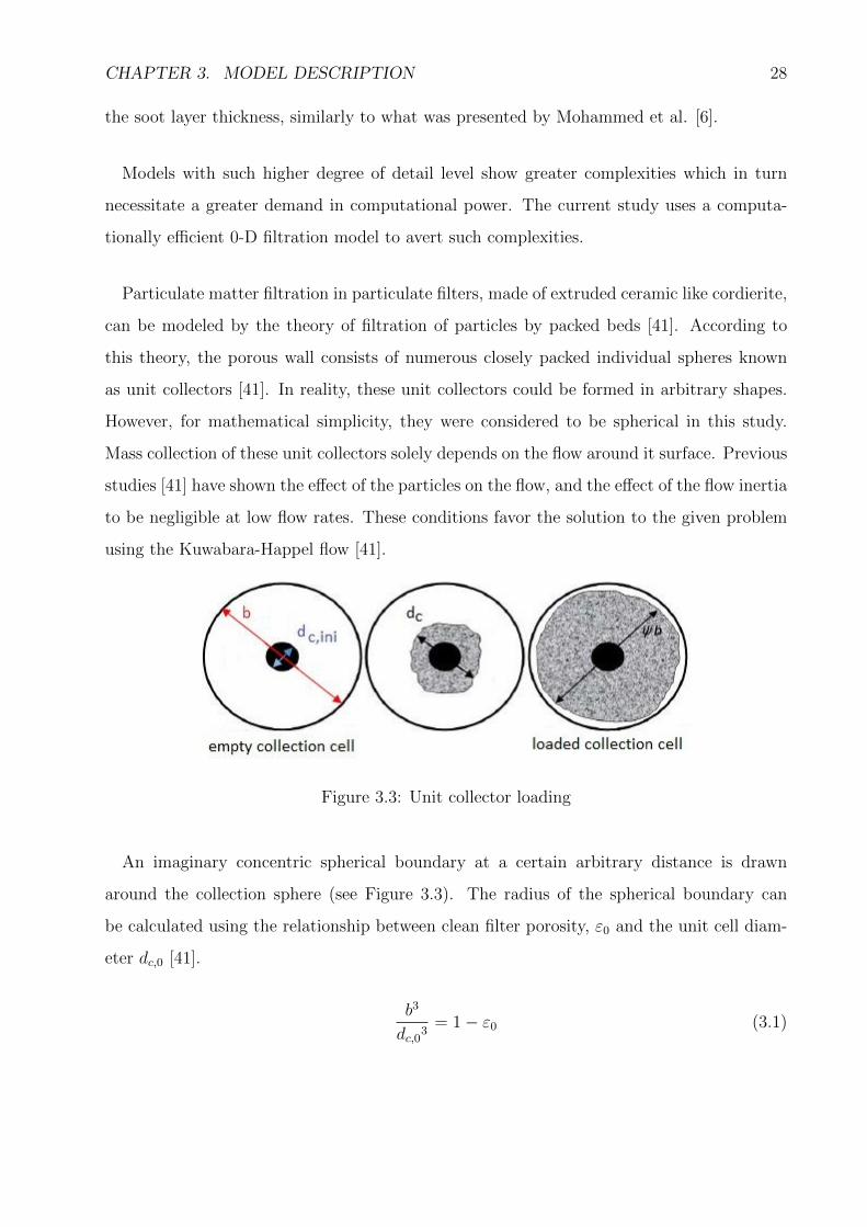
Particulate matter filtration in particulate filters, made of extruded ceramic like cordierite,
can be modeled by the theory of filtration of particles by packed beds [41]. According to
this theory, the porous wall consists of numerous closely packed individual spheres known
as unit collectors [41]. In reality, these unit collectors could be formed in arbitrary shapes.
However, for mathematical simplicity, they were considered to be spherical in this study.
Mass collection of these unit collectors solely depends on the flow around it surface. Previous
studies [41] have shown the effect of the particles on the flow, and the effect of the flow inertia
to be negligible at low flow rates. These conditions favor the solution to the given problem
using the Kuwabara-Happel flow [41].
Figure 3.3: Unit collector loading
An imaginary concentric spherical boundary at a certain arbitrary distance is drawn
around the collection sphere (see Figure 3.3). The radius of the spherical boundary can
be calculated using the relationship between clean filter porosity, ε0 and the unit cell diam-
eter dc,0 [41].
b3
dc,03= 1− ε0 (3.1)
CHAPTER 3. MODEL DESCRIPTION 29
A relationship for clean filter unit cell diameter (dc,0) can be derived assuming all the void
fraction is distributed over cylindrical pores of diameter, dpore and the external area of the
collectors matches the area of the surface of these pores [5].
dc,0 =3
2
(1− ε0
ε0
)dpore (3.2)
As exhaust gas flows through the filter, the porosity of the bed changes as particle accu-
mulation within the bed increases. However, not all the particles flowing into the filter get
trapped inside the filter. As described in Chapter 2, particle filtration mainly depends on
three aerosol deposition mechanisms: Brownian diffusion; inertial impaction and interception
collection.
The single sphere efficiency due to diffusional deposition of particles is defined as the ratio
of the rate at which particles diffuse to the sphere surface to that at which particles approach
a surface with the cross sectional area of the sphere [41]. Therefore filtration efficiency due
to diffusion could be derived incorporating the Kuwabara- Happel stream function [41].
ηD =7
2
ε
KPe−2/3 (3.3)
where Pe is Peclet number, ε is the loaded unit cell porosity and K is the Kuwabara hydro-
dynamic factor. Kuwabara hydrodynamic factor is given by
K = 2− ε− 9
5(1− ε)
13 − 1
5(1− ε)2 (3.4)
Peclet number for diffusion of particles is defined as
Pe =Ui dcDp
(3.5)
where Ui is undisturbed particle velocity, dc is unit collector diameter and Dp is particle dif-
fusion coefficient. The undisturbed flow rate across the channel Ui is related to the substrate
wall velocity uw and porosity ε as follows [7].

CHAPTER 3. MODEL DESCRIPTION 30
Ui =uwε
(3.6)
Diffusion coefficient is calculated assuming the Brownian motion of the particles and is
given by:
Dp =kBT
f(3.7)
where kB is the Boltzmann constant, T is absolute temperature of gas flowing through the
substrate wall and friction coefficient (f) is calculated based on Stokes law.
f = 3πµdp (3.8)
where dp is primary soot particle diameter and µ is dynamic viscosity. However, this only
applies to a rigid spherical particle which is further away from any surface. It is also a
known fact that the drag force experienced by the particle for a given velocity is less than
the predicted drag force estimated by the Stokes law. Cunningham slip correction factor
(Cf ), is used to correct the Stokes friction factor; hence the equation (3.8) can be re-written
as follows.
Dp =kBTCff
=kBTCf3πµdp
(3.9)
where kB is Boltzmann constant. Slip correction factor is given by [5]:
Cf = 1 +Kn(
1.257 + 0.4e−1.1Kn
)(3.10)
where Knp is the particle Knudsen number defined by:
Knp =2λ
dpore(3.11)

CHAPTER 3. MODEL DESCRIPTION 31
where dpore is pore diameter of the substrate wall and the mean free path λ of exhaust gas
is given by [5]:
λ =µ
P
√πRT
2M(3.12)
where ν is kinematic viscosity of exhaust gas, MW is the molecular weight of the exhaust
gas , R is universal gas constant P is atmospheric pressure and T is absolute temperature
of exhaust gas.
Single sphere interception efficiency of the particles trapped in a unit collector is modeled
by Lee et al. [41] as follows.
ηR =3
2
ε
K
R2i
(1 +R2i )s (3.13)
where Ri is the interception parameter
Ri =dpdc
(3.14)
where dc is collector diameter and s is given by [41]:
s =2− 2ε
3ε(3.15)
Overall collection efficiency for the single collector can thus be calculated assuming as a
combination of collection efficiencies associated with two filtration mechanisms:
ηDR = ηD + ηR − ηDηR (3.16)
where ηD and ηR represent the collection efficiencies due to diffusivity and direct interception,
CHAPTER 3. MODEL DESCRIPTION 32
respectively [5]. The overall collection efficiency of the substrate wall is given by Lee et al.
[41] as follows.
E = 1− exp(−3(1− ε)ηDRws
2εdc
)(3.17)
where ws is substrate wall thickness.
As exhaust gases flow through the wall, soot particles are eventually trapped by the unit
collectors which lead to a growth in unit collector diameter. The rate of mass trapped inside
the unit collector is equal to the product of mass flow rate through the wall and the overall
collection efficiency of the substrate wall. The unit collector diameter growth can thus be
calculated after defining a soot packing density (ρsoot,w) in the substrate wall [5].
dc(i, t) =
[(dc02
)3
+3
4π
mc(i, t)
ρsoot,w
] 13
(3.18)
where dc0 is initial unit collector diameter, mc is mass in one unit collector and ρw,soot is
soot packing density of the virtual soot layer. Having calculated the updated unit collector
diameter, modified porosity due to mass filtration can be calculated using equation (3.19).
ε(i, t) = 1−[dc(i, t)
dc,0
]3
(1− ε0) (3.19)
where ε0 is initial substrate porosity. Permeability change due to mass filtration is a function
of both unit collector diameter and the filter porosity. The local permeability of a loaded
filter k in terms of the clean filter permeability k0, is given by [5]:
k(i, t) = k0(i, t)
[dc(i, t)
dc,0
]2f(ε(i, t))
f(ε0)(3.20)
As wall filtration progresses, the microstructure space between unit collectors decreases
and eventually becomes less than the particle diameter. Under this circumstance, the filtra-

CHAPTER 3. MODEL DESCRIPTION 33
tion mechanism changes from wall filtration to cake filtration, during which the particles are
deposited on the surface and a particulate layer is formed. However, in reality, both wall
and cake filtration occurs simultaneously.
A mathematical control parameter known as the “partition coefficient (φ)”is used to de-
termine the fraction of incoming particle mass retained on the surface of the porous wall to
form a particulate layer. This parameter is expressed as follows. [5].
φ(t) =(dc,0(0, t)) 2 − dc,02
(ψ.b) 2 − dc,02(3.21)
Percolation factor ψ limits the amount of soot mass collected in a single cell unit collector
in its “fully loaded”state. When the local unit collector diameter reaches the ultimate unit
collector diameter (ψ.b ), the model no longer permits particles to flow through the substrate
wall; hence, all the mass is trapped on the cake layer. This parameter is used as a tuning
parameter in the model to control the amount of mass retained in the substrate wall.
As the cake layer grows on top of the substrate wall, the cake layer itself acts as a filter,
limiting the amount of particles entering the substrate wall. The mathematical formulation
of this phenomenon is extensively discussed in Mohammad et al. [6]. However, a detailed 1-D
filtration code developed by Cozzolini et al. [40] based on aforementioned references showed
that the cake filtration efficiency maintained at a constant value under the experimental
conditions in which the current model was tested. Hence, to avert additional complexities a
constant cake filtration efficiency Ecake of 0.9998 was adopted in to this model. Hence mass
separation between cake and wall layers can be further upgraded as follows.
mwall(t) = meng out[1− φ(t).Ecake] (3.22)
mcake(t) = meng out [φ(t).Ecake] (3.23)
where mwall and mcake are mass flow rates experienced by wall and cake layer respectively.
Engine out mass flow rate is given by meng out.

CHAPTER 3. MODEL DESCRIPTION 34
3.3 Regeneration Model
The particulate layer oxidation model under evaluation adopts the 2-layer approach de-
veloped by Konstandopoulos et al. [5] and Mohammed [6] (see Figure 3.4). Exhaust gas
flows through two layers: washcoat layer (w1) and the layer of particles deposited on the
washcoat (w2) or the cake layer.
Figure 3.4: Schematic of the particle deposition on filter channels
Some change in the internal structure of the deposit layer during reactions may be ex-
pected. However, these changes have not been studied; hence, are neglected in this model.
The soot particles residing in the washcoat layer are the closest to the catalytic coating of
the substrate wall. Hence, the particles in this region oxidize by both catalytic and thermal
means. Determining the limiting thickness wlimit of this imaginary boundary of the wash-
coat layer is a strenuous task. Published literature indicates that this thickness is confined to
about 10-30 µm [5]. Particles residing over this thickness are assumed to be oxidized only by
thermal means and have no effect on the presence of the wall catalytic layer. Mathematical
formulation of the particle separation between layer and layer 2 can be expressed as follows.
w1 = ws; w2 = 0 if ws<wlimit (3.24)
w1 = wlimit; w2 = ws − wlimit if ws ≥ wlimit (3.25)
3.3.1 Cake Regeneration Submodel
Three oxidation mechanisms occur in the cake layer:
(1) Thermal oxidation;

CHAPTER 3. MODEL DESCRIPTION 35
(2) Catalytic oxidation; and
(3) NO2 assisted thermal oxidation.
Soot oxidation due to presence of oxygen in exhaust gas at elevated temperatures (500-600◦C)
is described by thermal oxidation [5]. Soot oxidation at lower temperatures (≈ 450◦C) due
to presence of oxygen in exhaust gas with the assistance of Pt-doped catalytic washcoat layer
is referred to catalytic oxidation. Soot oxidation at lower temperatures (≈ 150◦C) due to
presence of NO2 in the exhaust gas is described as NO2 assisted thermal oxidation. The
dominance of each of these mechanisms depends heavily on the mass fractions of O2 and
NO2, and temperature at a given location in the DPF.
Reactions that occur in one phase are referred to as homogeneous reactions while reactions
that occur at interfaces between phases are heterogeneous reactions. Heterogeneous kinetic
reactions have to be considered since the transport process in the DPF occur between both
solid and gas phases. In the current model, chemical reactions in the gas phase are neglected
due to its short residence time in a DPF channel. The molar concentration of the reactant
species like O2 and NO2 inside a DPF channel is assumed to be constant throughout the
channel length for simplicity of calculation. It is a well understood fact that Diesel exhaust
particles are composed of carbon and many other hydrocarbon / hydrocarbon derived ma-
terials. In this model, as a general simplifying assumption, diesel soot particles are assumed
to be purely carbonaceous. Under this assumption, governing equations of soot oxidation
reactions can be expressed as follows.
C +O2 → CO2 (3.26)
C +1
2O2 → CO (3.27)
Aforementioned two reactions can be written as a global one step heterogeneous oxidation
reaction using a selectivity parameter as follows [29].
C +
(1− f
CO
2
)O2 → f
COCO + (1− f
CO)CO2 (3.28)

CHAPTER 3. MODEL DESCRIPTION 36
Carbon monoxide selectivity fCO in the equation (3.28) depends on the oxygen mole
fraction in the exhaust gas yO2 , thermal oxidation reaction rate constant kth, activation
temperature of carbon oxidation due thermal oxidation reactionEf1
R, and the gas temper-
ature in the wall Tw [29]. The mole fraction exponent n1 functions as a tuning parameter
of the model to control the amount of oxygen reacting with carbon particles to match up
with the experimental results. However, this value used in the model is coherent with the
published literature [29].
fCO
=1
1 + kthyn1
O2exp
(−Ef1
RTw
) (3.29)
The reaction rate constant kth follows the Arrhenius relationship.
kth = AthTn
wexp
(−EthRTw
)(3.30)
where Eth is activation energy of thermal oxidation and R is universal gas constant. In
equation (3.30), Ath is the pre-exponential factor of Diesel soot particle oxidation due to
thermal means andEth,O2
Ris the activation temperature of diesel exhaust oxidation due
thermal oxidation reaction. As described in the previous equation, temperature exponent n
serves as a tuning parameter to control the rate coefficient of the reaction.
Diesel particulate matter oxidation by NO2 primarily consists of two simultaneous reac-
tions: direct and cooperative oxidation in which one produces CO and the other produce
CO2 [42].
C + 2NO2 → CO2 + 2NO (3.31)
C +NO2 → CO +NO (3.32)
However, a one step global heterogeneous form of soot oxidation due to NO2 can be
expressed as thermal oxidation due to O2 incorporating a selectivity coefficient as follows [6].

CHAPTER 3. MODEL DESCRIPTION 37
C + (2− gCO
)NO2 → gCOCO + (1− g
CO)CO2 + (2− g
CO)NO (3.33)
The CO selectivity coefficient is modeled similarly to the thermal oxidation and is given
by [6].
gCO
=1
1 + kNO2yn3
NO2exp
(−Ef3
RTw
) (3.34)
The reaction rate constant for oxidation by NO2 is given in equation (3.35), [6]:
kNO2 = ANO2Tn
wexp
(−ENO2
RTw
)(3.35)
It is suggested by some authors that CO selectivity parameter may be neglected con-
sidering the dominance of the reaction given in equation (3.31) over the reaction given in
equation (3.32) [6]. In this model, the CO selectivity parameter was used in full form since
it does not arise any complications in its numerical implementation.
Particulate oxidation heavily depends upon the availability of O2 and NO2 mass at given
position. Assuming that the main reaction is a first order heterogeneous oxidation of carbon
and that diffusion is negligible compared to convection, the oxygen mass fraction YO2 and
the NO2 mass fraction YNO2 are conserved through the cake layer accordingly to equations
(3.36) and (3.37) [6]:
∂
∂x(ρwvwYO2) = −SpρwYO2kth
(1− f
CO
2
)(3.36)
∂
∂x(ρwvwYNO2) = −SpρwYNO2kNO2 (2− g
CO) (3.37)
where YO2,2 and YNO2,2 denote the oxygen mass fraction and the NO2 mass fraction enter-
ing the cake layer respectively, ρw is the exhaust density and vw denotes the gas velocity
approaching the soot layer.
CHAPTER 3. MODEL DESCRIPTION 38
The specific reactive surface area SP of diesel PM in the cake layer is given by Equation
(3.38):
Sp = Apρsoot,ck (3.38)
where Ap and ρsoot,ck are the area and density of diesel soot particles, respectively.
Total rate of O2 and NO2 depletion per unit wall surface area RthO2,2
and RNO2,2 can be
attained by integrating equations (3.39) and (3.40), respectively along the wall thickness.
RthO2,2
=
∫ w2
0
SpρwYO2kth
(1− fCO
2
)dx (3.39)
RNO2,2 =
∫ w2
0
SpρwYNO2kNO2 (2− gCO) dx (3.40)
As stated earlier in this section, the change in density and the velocity in the x direction
can be assumed negligible. With this assumption, O2 and NO2 depletion rates are given by
equations (3.41) and (3.42) respectively.
RthO2,2
= ρwvwYO2,2
[1− exp
(−Spkth
(1− fCO
2
)w2
vw
)](3.41)
RNO2,2 = ρwvwYNO2,2
[1− exp
(−SpkNO2 (2− gCO)w2
vw
)](3.42)
The O2 and NO2 depletion rates can be attributed to the consumption of the soot layer,
given by equation (3.43).
∂(ρsoot,ckw2)
∂t= − Mc
MO2
(RO2,2
1− fCO
2
)− Mc
MNO2
(RNO2,2
2− gCO
)(3.43)
where Mc, MNO2 and MO2 are molecular weights of carbon, nitrogen dioxide and oxygen
respectively.

CHAPTER 3. MODEL DESCRIPTION 39
3.3.2 Washcoat Regeneration Submodel
Diesel particulates trapped in the washcoat undergo both thermal and catalytic oxidation
and thus the oxygen depletion rates of the two paths have to be separately evaluated. But
first, the O2 and NO2 mass fractions leaving the cake layer and entering the washcoat layer
have to be calculated and can be expressed by:
YO2,1 = YO2exp
(−Spkth
(1− fCO
2
)w2
vw
)(3.44)
YNO2,1 = YNO2exp
(−SpkNO2 (2− gCO)w2
vw
)(3.45)
Stoichiometric equation for soot oxidation under catalytic means can be expressed similar
to equation (3.33). However, the selectivity parameter f′
COshould be modified to account
for oxidation at lower temperatures.
C +
(1−
f′
CO
2
)O2 ⇒ f
′
COCO +
(1− f ′
CO
)CO2 (3.46)
where selectivity parameter f′CO is given by
f′
CO=
1
1 + kcatyn2
O2exp
(−Ef2
RTw
) (3.47)
The reaction rate constant kcat follows the Arrhenius relationship:
kcat = AcatTn
wexp
(−EcatRTw
)(3.48)
The oxidation of the aforementioned paths were formulated by Konstandopoulos [5] in his
2-layer theory, using a soot oxidation fraction β. Due to low activation energy, soot particles
trapped in the washcoat layer primarily oxidize using the available O2 mass fraction and
then thermally oxidize with the remaining O2 mass fraction (1 − β). Thus, the O2 balance
equation for washcoat layer can be expressed as shown in equation (3.49).

CHAPTER 3. MODEL DESCRIPTION 40
∂
∂x(ρwvwYO2,1) = −SpρwYO2,1
[kth
(1− 1− fCO
2
)(1− β) + kcat
(1− 1− f ′CO
2
)β
](3.49)
Integration of the equation (3.49) over the washcoat thickness yields the total oxygen
depletion rate, RO2 ,total and is expressed in equation (3.50):
RtotalO2
= ρwvwYO2,1
[1− exp
(−Spk?w1
vw
)](3.50)
where,
k? = kth
(1− fCO
2
)(1− β) + kcat
(1− f
′CO
2
)β (3.51)
The CO selectivity and the soot oxidation fraction is then used to separate the catalytic
and thermal contributions from the total oxygen depletion rate.
RthO2,1
= RtotalO2
[kth(1− fCO
2
)(1− β)
k?
](3.52)
RcatO2,1
= RtotalO2
kcat(
1− f′CO
2
)β
k?
(3.53)
Upon integration of the NO2 balance equation, the following NO2 depletion rate in the
washcoat layer is obtained:
RNO2,1 = ρwvwYNO2,1
[1− exp
(−SpkNO2(2− gCO)w1
vw
)](3.54)
Considering the reaction stoichiometry, the transient change of the washcoat layer par-
ticulate thickness can then be expressed as follows.
∂(ρsoot,ckw1)
∂t= − Mc
MO2
(RthO2,1
1− fCO
2
)− Mc
MO2
RcatO2,1
1− f′CO
2
− Mc
MNO2
(RNO2,1
2− gCO
)(3.55)

CHAPTER 3. MODEL DESCRIPTION 41
The model requires a knowledge of the value of initial soot layer thickness along the
channel length in order to solve the initial value problems given in equations (3.43) and
(3.55). The initial soot layer thickness wb, was also considered to be constant along the
channel length even though it could be an axial space dependent value. This parameter was
determined using a process called “virtual conditioning” due to the fact that an aged filter
was used during experimental phase. “Virtual conditioning”will be discussed in detain in
Chapter 5.
3.3.3 Wall Regeneration Submodel
Wall regeneration submodel was formulated based upon the work of Mohommad et al.
[6]. Several authors have pointed out the importance of wall regeneration and its significant
contribution towards pressure drop, especially in CCRTs [6]. Wall regeneration modeling ap-
proach is same as in the previous two cases. Particles trapped inside the filter are formulated
to resemble a virtual particulate layer thickness, wwall. This thickness is calculated, similar
to unit cell theory, by defining a particulate packing density ρsoot,wall inside the substrate
wall.
wwall(z) =mwall(z)
Ddzρsoot,wall(3.56)
Local mass trapped inside the filter and the axial discretization length are represented
by mwall(z) and dz, respectively. Soot reside in the wall oxidizes only by thermal means.
This is mainly because the lack of data availability in the published literature related to the
catalytic penetration.
Considering the O2 and NO2 conservation equations for the substrate wall, respective mass
fractions exiting washcoat layer or entering substrate wall are given by:
YO2,wall = YO2,1 exp
(−Spk∗w1
vw
)(3.57)
YNO2,wall = YNO2,1 exp
(−SpkNO2 (2− gCO)w1
vw
)(3.58)

CHAPTER 3. MODEL DESCRIPTION 42
Depletion rates relating to the two species can be attained by integrating conservation
equations along the substrate wall thickness.
RO2,wall = ρwvwYO2,wall
[1− exp
(−Spkth
(1− fCO
2
)wwall
vw
)](3.59)
Similar to previous cases, using stoichiometry, the decay of the virtual wall layer thickness
can thus be expressed using the following equation.
∂(ρsoot,wallw1)
∂t= − Mc
MO2
(RO2,wall
1− fCO
2
)− Mc
MNO2
(RNO2,wall
2− gCO
)(3.60)
3.3.4 Wall Energy Balance
The one-dimensional temperature field in the monolith is described by the following as-
sumptions/mechanisms;
(1) Convection heat transfer between the substrate wall and the exhaust gas at the inlet and
the outlet channels;
(2) Conduction heat transfer through the substrate wall;
(3) Heat generation due to the exothermic soot oxidation; and
(4) Heat loss to the environment by convection.
The resulting formula can be expressed as follows:
(ρscpsws+ρsoot,ckcpp(w1+w2))∂Tw∂t
= h1(T1−Tw)+h2(T2−Tw)+Hreact+Hcond−Henvir (3.61)
where Cps is the heat capacity of the substrate wall, Cpp is the heat capacity of the particulate
matter, ρs and ρsoot,ck are the densities of the particulate matter and the substrate, Hreact
is the heat flux generated by chemical reaction of soot and Hcond heat flux losses due to
conduction through the substrate wall. The contribution of exothermic chemical reactions
depend on the O2 and NO2 depletion in washcoat and cake layers is given in equation (3.62):

CHAPTER 3. MODEL DESCRIPTION 43
Hreact =∆H th
MO2
[(1
1− fCO
2
)(RthO2,1
+RO2,2
)]+
∆Hcat
MO2
1
1− f′CO
2
(RcatO2,1
)+
∆HNO2
MNO2
[(1
2− gCO
)(RNO2,1 +RNO2,2)
](3.62)
where ∆H th,∆Hcat and ∆HNO2 are heats of reaction carbon oxidation due to thermal and
catalytic oxidation and NO2 reaction respectively. These heats of reactions solely depend
on their respective CO selectivity.
∆H th = fCO∆HCO + (1− fCO)∆HCO2 (3.63)
∆Hcat = f′
CO∆HCO + (1− f ′CO)∆HCO2 (3.64)
∆HNO2 = gCO∆HCO + (1− gCO)∆HCO2 + (2− gCO)∆HNO2 (3.65)
Conduction heat transfer through the substrate wall is calculated using the Euken [4]
formula given in equation (3.66)
Hcond = λsws∂2Tw∂z2
+ λp∂
∂z
(w1∂Tw∂z
)+ λp
∂
∂z
(w2∂Tw∂z
)(3.66)
where λs and λp are the thermal conductivity of substrate and the particulate layer respec-
tively.
Convection heat loss from the DPF can to the environment was also incorporated into
the model to re-create experimental conditions under which the model was validated. This
can be formulated with the use of conduction heat loss through DPF packaging and Newtons
law of cooling.
Henvir =(Tw − T0)
RtπDL(3.67)

CHAPTER 3. MODEL DESCRIPTION 44
Figure 3.5: Sectional view of DPF with thermal resistance parameters
Temperature of the ambient air is denoted by T0. The resultant thermal resistance Rt
across the DPF can be derived as follows.
Rt =log(rins
rf
)2πk1L
+log(
rcrins
)2πk2L
+1
2πrcLHex
(3.68)
where rins, rf and rc are outer radius of insulation layer, filter radius and outer radius of
canister respectively. The thermal conductivity between the filter and the insulation is k1
and the thermal conductivity between the insulation and the canister is k2.
The convective heat transfer coefficient for the DPF, Hex can be calculated using the
thermal conductivity kD of the filter can and the Nusselt number NuD and is given in
equation (3.69):
Hex =kDNuD
d(3.69)
Nusselt number for flow over a horizontal cylinder with uniform surface temperature for
a wide range of Rayleigh numbers, RaD is given by [43]:
NuD =
[0.6 +
0.387Ra16d
(1 + (0.559/Pr)9/16)8/27
]2
(3.70)

CHAPTER 3. MODEL DESCRIPTION 45
where, Pr is the Prandtl number and RaD is the Rayleigh number which can be expressed
as
RaD =gβth(Tw − T0)D3
αv(3.71)
In the above equation, g, β, α and ν denote gravitational acceleration, thermal expansion
coefficient, thermal diffusivity and kinematic viscosity, respectively.
As described earlier, the wall temperature is calculated by solving the second order
parabolic partial differential equation given in equation (3.61). Solving this equation re-
quires two boundary conditions and an initial condition. Two boundary conditions can be
attained by neglecting the heat losses from the front and rear faces of the monolith.
∂Tw∂z
(0, t) = 0 (3.72)
∂Tw∂z
(L, t) = 0 (3.73)
Initial wall temperature of the substrate, Tb, can be assumed constant throughout the
channel length, and equal to the engine out exhaust gas temperature when t = 0.
Tw(z, 0) = Tb (3.74)
3.3.5 Mass, Momentum and Energy Balance
This sub-section calculates the inlet and outlet channel temperatures and velocities over
channel length using conservation of momentum, mass and energy equations.
The exhaust gas mass balance states that, the change of the exhaust mass velocity is
equal to the exhaust mass velocity leaving the input channel via the porous wall. The mass

CHAPTER 3. MODEL DESCRIPTION 46
velocity in the inlet channel and the outlet channels are denoted by equations (3.75) and
(3.76), respectively.
∂(ρ1v1)
∂z= − 4
Dρwvw (3.75)
∂(ρ2v2)
∂z=
4
Dρwvw (3.76)
Considering the nature of the plug flow reactor following boundary conditions can be
imposed for inlet/outlet channels.
ρ1(0, t)v1(0, t) = ρeng(0, t)veng(0, t) (3.77)
ρ2(0, t)v2(0, t) = 0 (3.78)
ρ1(L, t)v1(L, t) = 0 (3.79)
The axial component momentum balance (z-momentum) of the exhaust gas is derived
using the Navier-Stokes equation considering incompressible flow of a Newtonian fluid. The
viscous drag plays a vital role as the gas velocities become zero at the wall ends. The friction
coefficient, F has a constant value of 28.454; thus, assuming fully developed laminar flow for
square cross sectional channel. The balance equation is the same for both channels.
∂P 1
∂z+∂(ρ1v1
2)
∂z= −Fµ(T 1)v1
D2(3.80)
∂P 2
∂z+∂(ρ2v2
2)
∂z= −Fµ(T 2)v2
D2(3.81)
The inlet and outlet channel energy balance equations are obtained considering the con-
vective heat transfer between exhaust gas and substrate wall. The enthalpy change due to
the flow across the particulate layer and wall was also considered. Convective heat transfer
of the channel dominates the conduction heat transfer hence the latter was neglected.

CHAPTER 3. MODEL DESCRIPTION 47
cpgρ1v1∂T 1
∂z=
4
D(h1 − cpgρwvw)(Tw − T 1) (3.82)
cpgρ2v2∂T 2
∂z=
4
D(h2 + cpgρwvw)(Tw − T 2) (3.83)
Inlet face of the DPF was considered to have the same temperature as the engine out
temperature and the initial spatial node of the outlet channel was considered to be equal to
the wall temperature [4].
T 1(0, t) = Teng(0, t) (3.84)
T 2(0, t) = Tw(0, t) (3.85)
The calculation of the convective heat transfer coefficients hi were calculated by the
relationship given by Bissett [4].
hi =Nu
D(cpg + a1)µ(Ti) (3.86)
The pressure difference can be described by Darcy’s law. Darcy’s law is a simple pro-
portional relationship between the instantaneous discharge rate through an isotropic porous
medium, viscosity of the fluid and pressure drop over a given distance. In this model, filter
wall velocities are relatively low and the Forchheimer contribution to the pressure drop is
considered to be negligible.
The overall pressure drop of a loaded catalyzed soot filter consists of several contributions: (1)
inlet/outlet cone pressure losses; (2) contraction/expansion pressure losses; (3) inlet/outlet
channel pressure losses and (4) wall and cake layer pressure losses. However, previous studies
[5, 44] have shown that all pressure losses, other than wall and cake layer pressure losses are
significant only at very high exhaust flow rates. Hence for the sake of generality, pressure
losses due to wall and particulate deposition layer are accounted in this model.
P 1 − P 2 =µ(Tw)wvw
kp+µ(Tw)wsvw
ks(3.87)

CHAPTER 3. MODEL DESCRIPTION 48
Outlet face of the DPF is considered to be held at atmospheric pressure Patm.
P 2(L, t) = Patm (3.88)

49
Chapter 4
Numercal Procedure
4.1 Solving the Boundary Value Problem
The model equations were numerically solved using finite difference methods adopting a
spatially uniform mesh with a grid spacing of 0.4 cm. The grid sensitivity was tested by
checking whether the results remain the same when a finer grid resolution was employed
and simulation time. Simulation time corresponding to a 200 second simulation with a given
grid resolution is illustrated in Table 4.1. According to the table, seventy discretized parts,
which was used in this model, gives the minimum simulation time. It is also worth noting
that simulation time depends on the cycle duration as the computer exhausts computational
resources to store calculated variables inside the program.
Table 4.1: Grid resolution comparison
Discretized Parts Simulation Time (sec)
10 Convergance Issue25 168.950 63.670 44.7100 79.1125 71.4150 86.3175 120.6200 145.7

CHAPTER 4. NUMERCAL PROCEDURE 50
The channel flow field and the energy balance equations [Eq:(3.75)-(3.88)] consist of two
point boundary value/initial value problems. All six of the non-linear, coupled ordinary
differential equations were simultaneously solved using “bvp4c”, an in built boundary layer
problem solver in Matlab. This solver implements a fourth order accurate Lobatto IIIa
formula. This routine requires the system of equations to be written as a system of first
order ODEs. Hence the aforementioned equations were re-written in the following form.
∂G1
∂z= −4
aGw (4.1)
∂G2
∂z=
4
aGw (4.2)
∂T1
∂z=
4
a
(h1 − cpgGw) (Tw − T1)
cpgρ1v1
(4.3)
∂T2
∂z=
4
a
(h1 + cpgGw) (Tw − T2)
cpgρ2v2
(4.4)
∂P1
∂z= −∂ (G2
1/ρ1)
∂z− Fµ(T1)v1
a2(4.5)
∂P2
∂z= −∂ (G2
2/ρ2)
∂z− Fµ(T2)v2
a2(4.6)
where
Gw =4
a
(P1 − P2)(µ(Tw)wkpρw
+ µ(Tw)ws
ksρs
) (4.7)
Gi = ρivi
Pi = ρRTi(4.8)

CHAPTER 4. NUMERCAL PROCEDURE 51
Even though “bvp4c”is an excellent routine to solve boundary value problems, the quality
of the solution heavily depends on the initial guess. A bad guess would result in inaccurate
solution, no solution or a solution which makes no sense. In this model, the values obtained
in the previous time step were considered as the initial guess values for the current time
step. This is a widely used technique to solve boundary value problems of this nature. The
relative error of the scheme was controlled to a tolerance of 10−3.
4.2 Solving the Initial Value Problem
A fourth order accurate Runge-Kutta method was employed to estimate the amount of
particulate oxidation inside the CCRT. The governing equations and the boundary conditions
related to the soot oxidation process was discussed in detail in the previous chapter. Classical
method of fourth order Runge-Kutta method is given by
yn+1 = yn + h
(k1
6+k2
3+k3
3+k4
6
)(4.9)
where
k1 = f(tn, yn)
k2 = f
(tn +
h
2, yn +
h
2k1
)k3 = f
(tn +
h
2, yn +
h
2k2
)k4 = f (tn + h, yn + hk3)
(4.10)
The k1, k2, k3 and k4 are known as the stages of the Runge-Kutta method. These
parameters correspond to different estimates for the slope of the solution. For instance, in
the case of washcoat regeneration, these parameters are given by following formulae.

CHAPTER 4. NUMERCAL PROCEDURE 52
k1 = − dt
ρsoot,cake
[αi1(1− eαi
2w1) + αi3(1− eαi2w1) + αi4(1− eαi
5w1)]
k2 = − dt
ρsoot,cake
[αi1(1− eαi
2(w1+0.5k1)) + αi3(1− eαi2(w1+0.5k1)) + αi4(1− eαi
5(w1+0.5k1))]
k3 = − dt
ρsoot,cake
[αi1(1− eαi
2(w1+0.5k2)) + αi3(1− eαi2(w1+0.5k2)) + αi4(1− eαi
5(w1+0.5k2))]
k4 = − dt
ρsoot,cake
[αi1(1− eαi
2(w1+k3)) + αi3(1− eαi2(w1+k3)) + αi4(1− eαi
5(w1+k3))]
(4.11)
where
αi1 =
(Mc
MO2
)kth(i)(1− β)ρw(i)vw(i)yi
k∗(i)αi2 = −Spk
∗(i)
vw
αi3 =
(Mc
MO2
)kcat(i)βρw(i)vw(i)yi
k∗(i)αi4 =
(Mc
MNO2
)ρw(i)vw(i)yiNO2
2− gCO(i)
αi5 = −SpkNO2(i)(2− gCO(i))
vw(i)
The filter wall energy balance was solved using a second order accurate Crank-Nicolson
scheme. The implemented formulation replaces all existing derivatives by a central difference
approximation, where the values of the old and new time steps are employed. Discretized
transformation of the Eq:(3.61) can be given as follows.
A1iTj+1wi−1
+ A2iTj+1wi
+ A3iTj+1wi+1
= B1iTjwi−1
+B2iTjwi
+B3iTjwi+1
+B4i (4.12)
where

CHAPTER 4. NUMERCAL PROCEDURE 53
A1i = −
(λpw
ji + λsws
)β
h2+ λp
[(wj+1i+1 − w
j+1i−1
2h
)β +
(wji+1 − w
ji−1
2h
)(1− β)
](β
2h
)A2i =
(ρpcppw
ji + ρpcpsws∆t
)+ 2
(λpw
ji + λsws
)( β
h2
)+
[ρpcpp
(wj+1i − wji
∆t
)+ hj1i + hj2i
]β
A3i = −
(λpw
ji + λsws
)β
h2− λp
[(wj+1i+1 − w
j+1i−1
2h
)β +
(wji+1 − w
ji−1
2h
)(1− β)
](β
2h
)
B1i =
(λpw
ji + λsws
)(1− β)
h2+ λp
[(wj+1i+1 − w
j+1i−1
2h
)β +
(wji+1 − w
ji−1
2h
)(1− β)
](1− β
2h
)B2i =
(ρpcppw
ji + ρpcpsws∆t
)− 2
(λpw
ji + λsws
)(1− βh2
)−
[ρpcpp
(wj+1i − wji
∆t
)+ hj1i + +hj2i
](1− β)
B3i =
(λpw
ji + λsws
)β
h2− λp
[(wj+1i+1 − w
j+1i−1
2h
)β +
(wji+1 − w
ji−1
2h
)(1− β)
](1− β
2h
)B4i =
(hj+1
1iT j+1
1i+ hj+1
2iT j+1
2i+Hj+1
react
)β +
(hj1iT
j1i
+ hj2iTj2i
+Hjreact
)(1− β)
(4.13)
Assuming the DPF was dicretized into “M ”number of nodes, the above scheme can be con-
veniently transformed in to a linear system with “M-2 ”or “k”number of equations as follows.
A12 +A22 A33 0
A13 A23 A33
A14 A24. . .
. . .. . . A3k−1
0 A1k A2k +A3k
T j+1w2
T j+1w3
T j+1w4
...
T j+1wk
=
(B12 +B22)T jw2 +B32Tjw3 +Bj
42
B13Tjw2 +B23T
jw3 +B33T
jw4 +Bj
43......
B1kTjwk + (B2k +B3k)T jwk +Bj
4k
The resulting sparse matrix was then solved using Gaussian elimination method. First
a set of row operations, called the forward sweep, uses each diagonal element as a pivot to
eliminate the elements of the matrix below the diagonal. Next, backward substitution was
used to obtain the solution vector starting from T jwkto T jw2
. Wall temperature related to
inlet and outlet nodes were calculated using the assumed boundary conditions at each time
step.

CHAPTER 4. NUMERCAL PROCEDURE 54
A time step of 0.1 seconds was employed for the time integration. During the FTP cycle,
experimental data was collected at 10 Hz data rate. Hence the same temporal time step
was selected when evaluating the simulated results even though the model is able perform
calculations with much lower temporal time steps. Moreover, the reduction of temporal time
step lead to an increase in simulation time. The current model took 40 minutes to simulate
a typical FTP cycle under the specified grid resolution on a Pentium 4 3.3 GHz machine.

55
Chapter 5
Experimental Setup and Procedures
5.1 Instrumentation and Laboratory Setup
The experimental data [39, 40] that was used to validate the developed DPF model was
collected at the Engine and Emissions Research Laboratory (EERL) at West Virginia Uni-
versity. Details of the experimental equipment and procedures are described in published
papers Mulone et al. [39] and Cozzolini et al. [40]. A very brief description [39, 40] of the
engine and exhaust aftertreatment system is given below.
A model year 2004 Mack MP7-355E heavy-duty diesel engine equipped with a high-
pressure loop exhaust gas recirculation system (EGR) and an exhaust aftertreatment system
consisting a diesel oxidation catalyst upstream of a Johnson-Matthey catalyzed diesel par-
ticulate filter (CCRT) were the primary components used in this study. Detailed engine
information and geometrical dimensions of the DOC/DPF is provided in Table 5.1 and Ta-
ble 5.2, respectively.
The testing procedure was based on the 40 CFR Part 1065 protocol. All diluted gaseous
sampling downstream the whole aftertreatment system were analyzed using the Horiba
MEXA 7200D system. Particulate matter characterization downstream the aftertreatment
system was quantified using the gravimetric method as outlined in 40 CFR Part 1065. Fil-
ters were weighed in an environmentally controlled clean room (Class 1000) using a Sartorius

CHAPTER 5. EXPERIMENTAL SETUP AND PROCEDURES 56
Table 5.1: Test engine manufacturer specifications
Model MACK MP7-355E
Configuration 6 Cylinders, InlineAspiration Sliding Nozzle Variable Turbocharger/IntercoolerInjection system Dual Solenoid Electronic Unit Injector (EUI)Maximum Torque 1844 Nm (1360 ft-lbs) @ 1200 RPMMaximum Power 265 kW (355 bhp) @ 1800 RPMDisplacement, L (cu-in) 11 (659)Compression Ratio 16.0:1Bore and Stroke, mm (in) 122.94 ×151.89 (4.84× 5.98)
Table 5.2: Geometrical dimensions of the DOC/DPF
Parameter DOC DPF
Diameter (in) 12 12Length (in) 5 12Cell Density (cpsi) 400 100Wall Thickness (mil) 4 12Clean Wall Porosity - 0.5
microbalance with an accuracy of 0.1 µg. The engine was connected to a General Electric
motoring/absorbing dynamometer capable of 700 hp for engine speed and load control to
perform steady state and transient test cycles.
Raw emissions were measured in addition to the diluted sampling. A Validyne P55D
differential pressure sensor was used to measure the differential pressure across the DPF,
which is critical for determining the soot loading quantity. A scale was placed directly
under the DPF-DOC system during the test. This allowed for quick determination of the
soot weight after detaching exhaust pipes and removing thermocouple/pressure transducer
harnessing following each test. The scale used for measuring the weight was an Ohaus CD-11
which presented a resolution of 0.5 grams while weighing the DOC/DPF system. Raw PM
mass concentration entering the DOC/DPF assembly was measured by using an AVL 483
micro soot sensor thus providing the model with an accurate estimation of carbonaceous
soot mass entering the filter.

CHAPTER 5. EXPERIMENTAL SETUP AND PROCEDURES 57
Table 5.3: Test point data
Test Mode R 10 (Soot Loading) R 100 (Regeneration)
Duration [h] 30 1.5Engine Load [ft-lbf] 105 1018Engine Speed [rpm] 1800 1800Fuel Flow Rate [kg/hr] 11.64 56.11CCRT Inlet Temp. [◦C] 226.5 483.8Intake Air Flow [scfm] 256.4 588.1
5.2 Experimental Procedure
The testing phase consisted of a 13 mode European Stationary Cycle (ESC) followed by
two FTP cycles and a regeneration cycle. The engine operated for 30 hours in the R10 mode
with intermittent periods of 15 minutes every 4 hour testing to perform DPF weighing and
engine refueling. Specifics of the test points is given in Table 5.3.
The engine was then operated on two FTP cycles to collect data in need to validate the
model under transient operation. FTP cycle was selected as a transient cycle mainly because
of the exhaust temperature observed during operation. In fact, as shown later in this work,
the cycle can be divided in two main parts depending on the average exhaust temperature.
In particular the first 10 minutes of the cycle correspond to an average temperature of 150◦C
while the last part of the test is characterized by high exhaust temperatures on the order of
400◦C. Hence it may be concluded that NO2 soot oxidation play a key role in the initial part
of the FTP cycle while the oxidation due to O2 is likely the most significant contributor to
filter regeneration rate during high temperature operation [45], thus giving an opportunity
to test the calibration of modeled soot oxidation on a wide range of operating points. Engine
speed and torque characteristics of the evaluated FTP cycle is illustrated in Figure 5.1 along
with exhaust flow rate, PM concentration, exhaust gas species concentrations (NOx/O2) and
CPF inlet temperature. Table 5.6 provides the averaged engine out brake specific emissions
over the two FTP cycles [40].

CHAPTER 5. EXPERIMENTAL SETUP AND PROCEDURES 58
Figure 5.1: FTP reference data, exhaust flow rate, exhaust gas specie concentrations andCPF inlet temperature [40]

CHAPTER 5. EXPERIMENTAL SETUP AND PROCEDURES 59
Table 5.4: Exhaust gas emissions before DOC and after DPF for soot loading mode, 1800rpm, 10% load [40]
R10 Mode Pre-DOC Post-DPF
HC [ppm] 118.4 2.7CO [ppm] 197 2.5NO [ppm] 123.9 52.5NO2 [ppm] 40.0 107.4NOx [ppm] 163.9 159.9NO/NO2 Ratio 3.09 0.49PM [mg/Sm3] 2 -
Table 5.5: Exhaust gas emissions before DOC and after DPF for soot regeneration mode,1800 rpm, 100% load [40]
R10 Mode Pre-DOC Post-DPF
HC [ppm] 37.7 0CO [ppm] N/A 0NO [ppm] 361.4 335.0NO2 [ppm] 116.8 96.6NOx [ppm] 478.2 431.6NO/NO2 Ratio 3.09 3.47PM [mg/Sm3] 13 -
Table 5.6: The average engine out brake specific emissions during two FTP cycles
Particle/Gaseous Specie Brake Specific Emissions
HC [g/bhp-hr] 0.098CO [g/bhp-hr] 1.332NO [g/bhp-hr] 2.33NO2 [g/bhp-hr] 0.06NOx [g/bhp-hr] 2.39PM [g/bhp-hr] 0.0648

60
Chapter 6
Results and Discussion
The experimental results reflected in this study were obtained with an aged CPF; hence,
the author did not have access to some key initial DPF parameters such as wall permeability
and existing soot layer thickness along the channel before running the first test cycle. Thus,
the previously validated 1-D model [40] was used to determine these parameters using a
process called virtual conditioning.
Virtual conditioning procedure creates a loading condition representative of the given
physical state of the filter using a random sequence of loading and regeneration events [14].
Assuming the properties of a clean DPF, the conditioning procedure starts with a certain
selected tuning parameters and applies a random sequence of loading cycles until it reaches
the pressure drop value of the first experimental cycle. Then, the model is virtually exposed
to the same physical conditions that existed during the experimental phase. If the condi-
tioned filter is capable of mimicking the results of first loading cycle, then the simulation
is moved to the next loading cycle. If the discrepancy of the pressure drop results between
the simulated and the experimental values are out of ±0.1kPa, the tuning parameters are
adjusted and the validation procedure is started again from the beginning.
The decision of using the 1-D model to provide the loading cycle under investigation was
based mainly on required computational timings. As described in Chapter 4, the simulation
time of the current model is approximately twice that of the actual cycle duration. The

CHAPTER 6. RESULTS AND DISCUSSION 61
Table 6.1: Model tuning parameters and constants
Symbol Description Value Units
Eth,O2/R O2 Thermal Activation Temperature 1.55E+4 KEcat,O2/R O2 Catalytic Activation Temperature 1.42E+4 KENO2/R NO2 Activation Temperature 1.03E+4 KAth O2 Thermal Rate Constant 25.08 m/sKAcat O2 Catalytic Rate Constant 2.84 m/sKANO2 NO2 Rate Constant 2.9 m/sKSp Soot Specific Area 5.5E+7 1/mρsoot,w Wall Soot Packing Density 6.8 kg/m3
ρsoot,cake Cake Soot Packing Density 35 kg/m3
k0 Soot Wall Clean Permeability 3.4E-13 m2
ksoot Cake Layer Permeability 3.6E-14 m2
ψ Wall Filtration Filing Parameter 0.83 -w0 Initial Deposit Thickness 1.718E-5 m
numerical conditioning procedure requires application of numerous loading cycles each lasting
4 hours. The use of 1-D model could drastically reduce this computational burden as it could
simulate the same cycle in approximately 1/5th of the actual cycle duration. The reliability
of the 1-D code was validated elsewhere [39, 40]. Once the 1-D model produces satisfactory
pressure drop values relevant to the first loading cycle, the 2-D model assigns those flow
conditions, wall filtration characteristics and temperature profiles as its initial conditions,
and runs the succeeding loading cycles.
The tuning parameters used in the current model are shown in Table 6.1. It is noteworthy
that same tuning parameters used in the 1-D model are assumed to catch possible deviations
between results. These parameters fall in the ranges specified in similar models available in
the published literature [5],[29].
6.1 Steady State Cycle Analysis
The steady state particle loading experiments at different loading conditions were summa-
rized in Table 5.3. The collected CPF data include engine exhaust volumetric flow rate, inlet
and outlet temperatures, pressure drop, PM concentration, gaseous emission concentrations

CHAPTER 6. RESULTS AND DISCUSSION 62
and inlet particle size distribution. The accumulated mass inside the DPF was measured by
pre-weighing and post weighing the DPF after each cycle.
Figure 6.1: Experimental pressure drop of the DPF during the loading cycle
Pressure drop profile acquired during the loading phase is illustrated in Figure 6.1. Pres-
sure drop data collected between 18-22 hours were not available for analysis due to an error
in the data acquisition system. Typical pressure drop characteristics related to a clean DPF
shows a more gradual and rounded profile during the initial phase of loading. The rounded
profile results in initial deposition of soot particles which leads to a gradual increase in unit
collector diameters inside the porous wall. Even a small amount of mass could lead to a
sudden increase of pressure drop across the filter wall. However, this characteristic behavior
is not present in Figure 6.1 due to the use of an aged filter. In the given scenario, pressure
drop is determined mostly by the growth of the particulate layer thickness; thus linearly
increase with time.
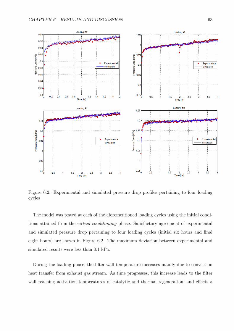
CHAPTER 6. RESULTS AND DISCUSSION 63
Figure 6.2: Experimental and simulated pressure drop profiles pertaining to four loadingcycles
The model was tested at each of the aforementioned loading cycles using the initial condi-
tions attained from the virtual conditioning phase. Satisfactory agreement of experimental
and simulated pressure drop pertaining to four loading cycles (initial six hours and final
eight hours) are shown in Figure 6.2. The maximum deviation between experimental and
simulated results were less than 0.1 kPa.
During the loading phase, the filter wall temperature increases mainly due to convection
heat transfer from exhaust gas stream. As time progresses, this increase leads to the filter
wall reaching activation temperatures of catalytic and thermal regeneration, and effects a

CHAPTER 6. RESULTS AND DISCUSSION 64
reduction in soot layer thickness. According to Darcy’s law, soot layer thickness is directly
proportional to filter pressure drop which leads to a decrease in the rate of pressure drop. This
effect can be seen in Figure 6.2. The gradients of the pressure drop curve during the initial
two cycles are considerably higher than that of the last two loading cycles. Furthermore, the
non-linear behavior seen in the initial part of each loading cycle should not be misunderstood
as deep bed filtration, but as an effect due to transient increment of filter temperature.
Figure 6.3 represents this transient temperature increment and testifies to the model ca-
pability in tracking exit temperature of the DPF. The maximum deviation between exper-
imental and simulated temperature data was ± 3K. As shown in Figure 6.4, highest wall
temperature values occur near the filter inlet face. It is impossible to attain a constant tem-
perature profile along filter length other than in the initial time step due to environmental
heat loss.
Figure 6.3: Experimental and simulated DPF outlet temperature of the 8th loading cycle

CHAPTER 6. RESULTS AND DISCUSSION 65
Figure 6.4: Experimental and simulated DPF outlet temperature of the 8th loading cycle
Having validated performance over a range of loading cycles, the model was then used to
predict missing filter pressure drop data during 18-22 hour time duration (6th loading cycle).
Engine volumetric flow rate, engine out temperature, PM concentration and exhaust gas
specie concentrations were assumed same as in the previous loading cycle. This is a valid
assumption considering the steady state engine operation. Changing filter properties such
as initial soot layer thickness and initial filter wall temperature were determined from the
data acquired in the last time step of the previous loading cycle. The predicted pressure
drop values from the model produced satisfactory results and is given by Figure 6.5. It is
interesting to note that the initial pressure drop value of the 6th loading cycle is in agreement
with the final pressure drop value of the 5th loading cycle and final pressure drop value of
the 6th loading cycle is in agreement with the initial pressure drop value of the 7th loading
cycle. Moreover, the gradient of the pressure drop curve is lower than that of the 5th loading
cycle which is in agreement with the effect of pressure drop on regeneration.

CHAPTER 6. RESULTS AND DISCUSSION 66
Figure 6.5: Model predicted filter pressure drop during 18-22 hour time duration during theloading phase
Figure 6.6 depicts the simulated evolution of the mean cake thickness on the filter wall
surface over a four hour loading cycle. As seen in the figure, the soot layer thickness evolution
is noteworthy at the two ends of the filter close to the inlet and the outlet of the channel.
This is a consequence of the profiles of the filter wall velocity. Higher soot layer thicknesses
at the ends of the filter provide higher resistance for exhaust gas to flow through the wall
in comparison to mid-regions of the filter. Consequently, over time, an increase in wall flow
velocity magnitude in the mid region can be observed as illustrated in Figure 6.7. This
trend may transform the wall velocity to a more uniform profile after several hours of engine
operation.
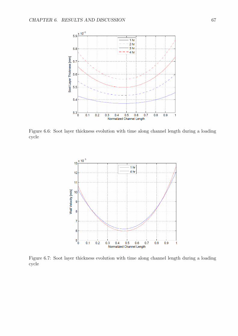
CHAPTER 6. RESULTS AND DISCUSSION 67
Figure 6.6: Soot layer thickness evolution with time along channel length during a loadingcycle
Figure 6.7: Soot layer thickness evolution with time along channel length during a loadingcycle

CHAPTER 6. RESULTS AND DISCUSSION 68
Figure 6.8 presents inlet and outlet channel velocity profiles during a loading cycle. The
inlet channel velocity reaches maximum at the entrance of the channel and it is reduced to
zero at the end plug. Similarly, the outlet channel velocity gradually increases, in sympathy
with the inlet velocity, across the channel length as the exhaust gas flows through the wall.
The shape of these profiles change from linear to an “S”shape as the filter gets filled with
more soot since the gradient of those profiles are directly proportional to wall velocity.
Figure 6.8: Soot layer thickness evolution with time along channel length during a loadingcycle
The model predicted particulate mass evolution with time during the loading phase is
illustrated in Figure 6.9. The figure shows satisfactory agreement between experimental and
simulated results. The maximum deviation of the two results is 3.47g which was shown
during the last few loading cycles. Use of the zeroth dimensional (0D) filtration model could
be one reason for this discrepancy. A 0D filtration model accounts for only one filtration
efficiency considering the the whole thickness of the model. On the other hand a more
advanced one dimensional (1-D) filtration model produces multiple filtration efficiencies as
it divides the filter wall thickness into several slabs. This would lead the latter model to
produce higher filtration efficiencies whilst retaining more mass in the filter wall than the

CHAPTER 6. RESULTS AND DISCUSSION 69
0D model. However, as discussed in earlier chapters, such a model would require a strenuous
computational effort. It is noteworthy to point out that even a 1-D filtration model could
be subjected to an mass error tolerance of ± 2.83g [40]. Moreover, low accuracy (±0.5g) of
the scale used in this study could be another reason for the reported mass discrepancy.
Figure 6.9: Experimental and simulated DPF soot mass comparison during the loading phase
6.2 Transient Cycle Analysis
Input variables related to the evaluated FTP cycles were given in Figure 5.1. The tuning
parameters given in Table 6.1 were kept unchanged even during the transient cycles as the
capabilities towards real time applications have to be demonstrated in this context.
Figure 6.10 shows a satisfactory agreement between the experimental and the simulated
pressure drop of the DPF. The model is able to capture the pressure drop characteristics
during heavily transient regimes with a high degree of detail. The accuracy of DPF pressure
drop prediction by the 2-D model was further evaluated by plotting experimental pressure
drop against simulated data (see Figure 6.11). The coefficient of determination corresponding
to this graph was 0.9883 and is satisfactory considering the transient nature of the cycle.

CHAPTER 6. RESULTS AND DISCUSSION 70
Figure 6.10: Pressure drop comparison between experimental and numerical data over anFTP cycle
Figure 6.11: Experimental vs. simulated DPF pressure drop
Mass balance of the DPF during the FTP cycle is depicted in Figure 6.12. Even though
NO2 assisted regeneration is present in the initial phase of the FTP cycle, the contribution
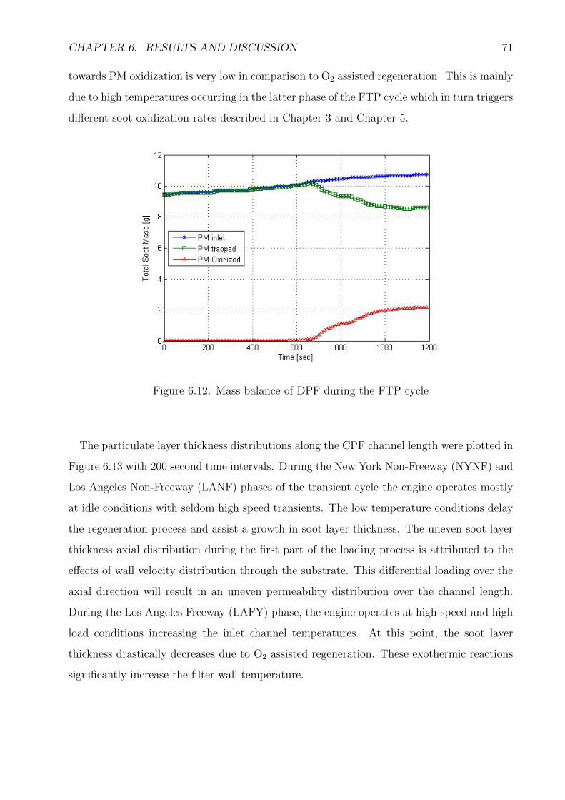
CHAPTER 6. RESULTS AND DISCUSSION 71
towards PM oxidization is very low in comparison to O2 assisted regeneration. This is mainly
due to high temperatures occurring in the latter phase of the FTP cycle which in turn triggers
different soot oxidization rates described in Chapter 3 and Chapter 5.
Figure 6.12: Mass balance of DPF during the FTP cycle
The particulate layer thickness distributions along the CPF channel length were plotted in
Figure 6.13 with 200 second time intervals. During the New York Non-Freeway (NYNF) and
Los Angeles Non-Freeway (LANF) phases of the transient cycle the engine operates mostly
at idle conditions with seldom high speed transients. The low temperature conditions delay
the regeneration process and assist a growth in soot layer thickness. The uneven soot layer
thickness axial distribution during the first part of the loading process is attributed to the
effects of wall velocity distribution through the substrate. This differential loading over the
axial direction will result in an uneven permeability distribution over the channel length.
During the Los Angeles Freeway (LAFY) phase, the engine operates at high speed and high
load conditions increasing the inlet channel temperatures. At this point, the soot layer
thickness drastically decreases due to O2 assisted regeneration. These exothermic reactions
significantly increase the filter wall temperature.

CHAPTER 6. RESULTS AND DISCUSSION 72
Figure 6.13: Soot layer thickness distribution along normalized CPF channel length (above);Temporal decay of soot layer thickness at different axial locations (below)
Moreover, at any given time, the front face of the CPF is exposed to the highest local
temperature and gradually decreases as exhaust gases proceed to end of the channel, mainly
due to convective heat loss to the filter wall. This leads to a decrease in the rate of regen-
eration towards the end of the channel as shown in Figure 6.13 thus collecting more soot at
the end of the filter in comparison to the front end. According to Figure 6.13, FTP cycle

CHAPTER 6. RESULTS AND DISCUSSION 73
can be regarded as a regenerating and loading cycle when viewing from the front section and
the rear end of the DPF respectively. High temperature is generally maintained through the
second NYNF phase of the transient cycle due to thermal inertia and continues to further
consume the soot layer thickness.
6.3 1-D and 2-D Model Comparison
One of the objectives of this study was to use the model under investigation to asses
the validity of the assumptions made in the 1-D model. This task will be carried out by
comparing the results obtained by the two models related to both steady state and transient
engine operating conditions.
6.3.1 Steady State Cycle Results Comparison
Pressure drop estimation is one of the main performance parameters of this model. Co-
efficient of determination values obtained from model predicted and experimental pressure
drop values for six loading cycles are given in Table 6.2.
Table 6.2: Coefficient of determination comparison relevent to 1-D and 2-D model predictedand experimental pressure drop during the 30 hour loading phase
Cycle Exp.vs.1-D Exp.vs.2-D
Loading 1 0.9458 0.9349Loading 2 0.9568 0.9631Loading 3 0.8015 0.8893Loading 5 0.9438 0.9343Loading 7 0.9459 0.9541Loading 8 0.7151 0.9139
As seen in the Table 6.2, both 1-D and 2-D models produce satisfactory agreements with
the experimental pressure drop values during steady state engine operation conditions. One
of the main parameters which control filter pressure drop are wall and soot layer permeability
and soot layer thickness. The 1-D model uses a cake filtration model and a continuous wall

CHAPTER 6. RESULTS AND DISCUSSION 74
soot filtration model. On the other hand, 2-D model uses a constant cake filtration efficiency
and a 0-D wall soot filtration model. However, in the given engine operating conditions, cake
filtration efficiencies were almost constant and fairly close average cake filtration efficiency
used in the 2-D model. Moreover, the change in wall permeability due to the use of 1-
D continuous filtration model and 0-D filtration model was very small due to the absence
of the deep bed filtration phase. Hence, the soot layer thickness predictions given by the
two models becomes to the main determination factor contributing to the discrepancy of
pressure drop predictions between the two models. The evolution of the soot layer thickness
is directly proportional to filter wall velocity during a loading cycle when regeneration effects
are minute. Calculated filter wall velocities at four difference axial positions using 2-D model
and 1-D model predicted filter wall velocity is given in Figure 6.14.
Figure 6.14: Wall velocity distribution comparison along filter length
As illustrated in Figure 6.14, length averaged filter wall velocity given by the 2-D model
is approximately equal to the 1-D model predicted filter velocity. Hence one may concluded
that, the average soot layer thickness given by the 2-D model is approximately equal to
the soot layer thickness given by the 1-D model and thus explain similar pressure drop
predictions given by the two models.

CHAPTER 6. RESULTS AND DISCUSSION 75
Experimentally measured mass end of each cycle along with 1-D and 2-D model DPF mass
estimations are given in Figure 6.15. Mass predictions of the two models agrees well with
each other and the maximum discrepancy between mass predictions was 0.98g.
Figure 6.15: 1-D and 2-D DPF soot mass prediction comparison
The 1-D model assumes a constant filter wall temperature along the filter length. However,
in reality, filter wall shows a temperature distribution along the filter length as implemented
in the 2-D model. As will be shown later in the transient model comparison, treating
wall temperature as a distribution becomes significant during soot layer decay due to O2
assisted thermal and catalytic regeneration. However, these regeneration mechanisms initiate
typically at temperatures above 500K. The maximum wall temperature attained during
the whole loading phase was 495K. At these temperatures soot layer decays due to NO2
assisted regeneration which is a far less powerful regeneration mechanism compared to the
aforementioned. This effect describes the lower soot mass predictions from 2-D model in
comparison to 1-D model during the last few loading cycles.

CHAPTER 6. RESULTS AND DISCUSSION 76
6.3.2 Transient Cycle Results Comparison
As seen in the Table 6.3, both 1-D and 2-D models produce satisfactory agreements with
the experimental pressure drop values also during transient engine operation conditions.
Both models have shown exceptional ability to accurately capture pressure drop values during
highly transient regions of the cycle.
Table 6.3: Coefficient of determination comparison relevent to 1-D and 2-D model predictedand experimental pressure drop during transient cycles
Cycle Exp.vs.1-D Exp.vs.2-D
FTP 1 0.9882 0.9883FTP 2 0.9884 0.9878
During the first half period of the FTP cycle, both models report more or less the same
amount of DPF PM loading. During this phase, the temperature difference between inlet
and the outlet face of the DPF is small and the temperature at any given section of the DPF
can be effectively represented by the 1-D model. However, during LAFY phase the DPF is
subjected to high temperatures and the DPF wall temperature gradient cannot be further
regarded as a constant. At this point, the front of the DPF burns much more soot mass
than the back, and temperature gradient of the wall may not further be modeled by a single
temperature. Hence, 1-D model reports more soot mass in comparison to the 2-D model and
is reflected in Figure 6.16.

CHAPTER 6. RESULTS AND DISCUSSION 77
Figure 6.16: Total soot mass predictions of 1-D and 2-D models
Figure 6.17: Temperature distribution variation at different axial locations
Temperature distribution variation at different axial locations further defends the effect
seen in Figure 6.16. As seen in Figure 6.17, 2-D model display significantly higher wall
temperature distributions in comparison to the 1-D model. Varying wall temperature distri-
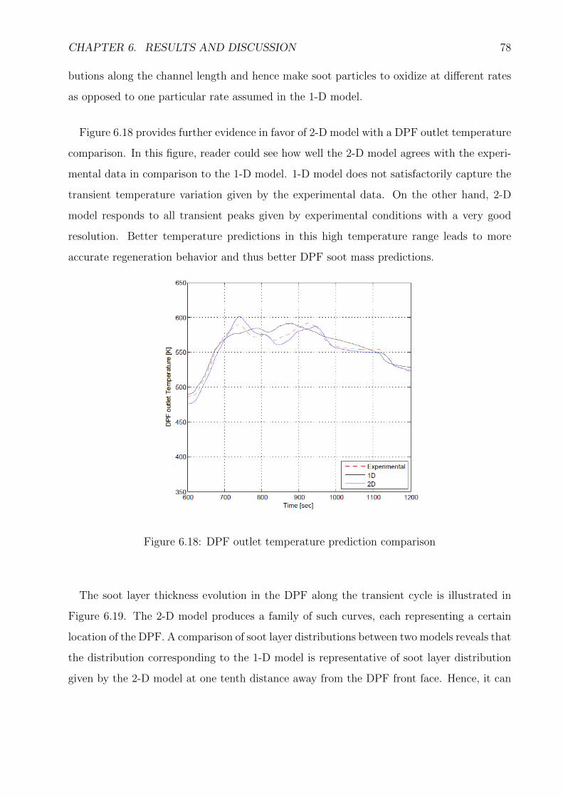
CHAPTER 6. RESULTS AND DISCUSSION 78
butions along the channel length and hence make soot particles to oxidize at different rates
as opposed to one particular rate assumed in the 1-D model.
Figure 6.18 provides further evidence in favor of 2-D model with a DPF outlet temperature
comparison. In this figure, reader could see how well the 2-D model agrees with the experi-
mental data in comparison to the 1-D model. 1-D model does not satisfactorily capture the
transient temperature variation given by the experimental data. On the other hand, 2-D
model responds to all transient peaks given by experimental conditions with a very good
resolution. Better temperature predictions in this high temperature range leads to more
accurate regeneration behavior and thus better DPF soot mass predictions.
Figure 6.18: DPF outlet temperature prediction comparison
The soot layer thickness evolution in the DPF along the transient cycle is illustrated in
Figure 6.19. The 2-D model produces a family of such curves, each representing a certain
location of the DPF. A comparison of soot layer distributions between two models reveals that
the distribution corresponding to the 1-D model is representative of soot layer distribution
given by the 2-D model at one tenth distance away from the DPF front face. Hence, it can
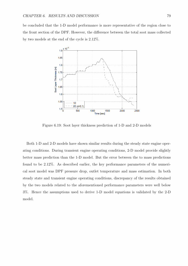
CHAPTER 6. RESULTS AND DISCUSSION 79
be concluded that the 1-D model performance is more representative of the region close to
the front section of the DPF. However, the difference between the total soot mass collected
by two models at the end of the cycle is 2.12%.
Figure 6.19: Soot layer thickness prediction of 1-D and 2-D models
Both 1-D and 2-D models have shown similar results during the steady state engine oper-
ating conditions. During transient engine operating conditions, 2-D model provide slightly
better mass prediction than the 1-D model. But the error between the to mass predictions
found to be 2.12%. As described earlier, the key performance parameters of the numeri-
cal soot model was DPF pressure drop, outlet temperature and mass estimation. In both
steady state and transient engine operating conditions, discrepancy of the results obtained
by the two models related to the aforementioned performance parameters were well below
3%. Hence the assumptions used to derive 1-D model equations is validated by the 2-D
model.

80
Chapter 7
Conclusions
The current study extended the previously validated 1D filtration and regeneration model
in to two dimensional space with the intention analyzing the given problem in a more de-
scriptive manner. The numerical investigation of the two dimensional numerical soot model
was performed for both steady state and transient engine operating conditions and results
presented here show satisfactory agreement with experimental data. The model is capable of
representing the evolution of the DPF back pressure and PM content along the filter channel.
According to the discussed results, following conclusions can be drawn.
• Satisfactory correlation between the experimental and simulated pressure drop was
obtained (R2= 0.88 for steady state and R2= 0.98 for transient) for both steady state
and transient engine operating conditions. This is one of the key performance metrics
of the current model.
• The soot layer thickness evolution is noteworthy at the two ends of the filter close to
the inlet and the outlet of the channel. Hence over time wall flow velocity magnitude
in the mid region increases and may eventually lead to a constant soot layer thickness
distribution across filter length.
• The model is capable of tracking DPF soot mass with a satisfactorily maximum dis-
crepancy of 3.47g during steady state cycles.
• The 2D model is able to capture the regeneration phase of the FTP more descriptively

CHAPTER 7. CONCLUSIONS 81
than the 1D model. However, the reported discrepancy of the total soot mass estimated
by two models was 2.12%.
• The distribution corresponding to the 1D model is representative of soot layer distri-
bution given by the 2D model at one tenth distance away from the DPF front face.
• 1D model representation is effective toward PM loading prediction, although presenting
considerable axial effects at higher DPF temperature.

82
Appendix A
Model Validation Using Bissett Model
In this Appendix, DPF pressure drop and mass retained results were compared with results
published in Bissett et al. [4]. The 2-D model showed god agreement with the pressure drop
data given by Bissett et al. [4]. Figure A.1 shows that the two sets of results were within ±
0.25 kPa. The maximum difference in mass retained in the filter as calculated by the models
(see Figure A.2) was less than 10 mg.
Figure A.1: DPF pressure drop validation using Bissett model

APPENDIX A. MODEL VALIDATION USING BISSETT MODEL 83
Figure A.2: Mass retained in the DPF validation using Bissett model

84
References
[1] Kitagawa J., Hijikata T. and Yamada S., Electric Heating Regeneration od Large Wall-Flow type DPF, SAE Technical paper 910136, 1991.
[2] Walton F.B., Hayward P.J. and Wren D.J., Controlled Energy Deposition in Diesel Par-ticulate Filters During Regeneration by Means of Microwave Irradiation, SAE TechnicalPaper 900327, 1990.
[3] Gautam M., Popuri S., Rankin B. and Seehra M., Development of a Microwave AssistedRegeneration System for a Ceramic Diesel Particulate System, SAE Technical Paper1999-01-3565, 1999.
[4] Bissett E. J., Thermal Regeneration of Particle Filters with Large Conduction,Mathematical Modeling, Vol. 6, pp.1-18, 1985.
[5] Konstandopoulos A.G., A., Kostoglou, M., Skaperdas, E., Papaioannou, E., ZarvalisD. and Kladopoulou E., Fundamental Studies of Diesel Particulate Filters: TransientLoading, Regeneration and Aging, SAE Technical Paper 2000-01-1016, 2000.
[6] Mohammed H., Triana A.P., Yang S.L. and Johnson J.H., An Advanced 1D 2-Layer Cat-alyzed Diesel Particulate Filter Model to Simulate: Filtration by the Wall and ParticulateCake, Oxidation in the Wall and Particulate Cake by NO2 and O2 and Regeneration byHeat Addition, SAE Technical Paper 2006-01-0467, 2006.
[7] Konstandopoulos A.G., Kostoglou M., Vlachos N. and Kladopoulou E., Ad-vances in the Science and Technology of Diesel Particulate Filter Simulation,Advances in Chemical Engineering, Vol.33, pp.213-294, 2007.
[8] Rumminger, M., Zhou, X., Balakrishnan K., Edgar, B., and Ezekoye, O., RegenerationBehavior and Transient Thermal Response of Diesel Particulate Filters, SAE TechnicalPaper 2001-01-1342, 2001.
[9] Khan M. R. and Shamim T. A Numerical Investigation of the RegenerationCharacteristics of Diesel Particulate Filters under Simulated Transient ExhaustConditions, Proceedings of the Institution of Mechanical Engineers, Part D: Journal ofAutomobile Engineering, pp.2469-2485, 2008.
[10] Kandylas I.P. and Koltsakis G.C., Simulation of Continuously Re-generating Diesel Particulate Filters in Transient Driving Cycles,

REFERENCES 85
Proceedings of the Institution of Mechanical Engineers, Part D: Journal of AutomobileEngineering, pp.591-606, 2002.
[11] Bennett S., MODERN DIESEL TECHNOLOGY:DIESEL ENGINES, New York: Del-mar, 2010.
[12] Heywood J.B., INTERNAL COMBUSTION ENGINE FUNDAMENTALS, New York:McGraw Hill, Inc., 1988.
[13] U.S. Environmental Protection Agency. Emission Standards Reference Guide. July 4th2011. http://www.epa.gov/otaq/standards/heavy-duty/hdci-exhaust.htm.
[14] U.S. Environmental Protection Agency. An Introduction to Indoor Air Quality (IAQ).July 4th 2011. http://www.epa.gov/iaq/co.html.
[15] Carcinogenic Effects of Exposure to Diesel Exhaust, Current Intelligence Bulletin 50,Publication No. 88-116, pp.548-159, 1988.
[16] Eastwood P., PARTICULATE EMISSIONS FROM MOTOR VEHICLES, New Jersey:Wiley and Sons Ltd, 2008.
[17] Zheng M., Reader G.T. and Hawley J.G., Diesel Engine Exhaust Gas Recirculation-a review on advanced and novel concepts, Energy Conversion and Management, Vol.45,pp.883-900, 2004.
[18] Platinum Today. Autocatalyst. 4th July 2011. http://www.platinum.matthey.com/applications/autocatalyst/
[19] Nova I., Lietti L., Tronconi E. and Forzatti P., Dynamics of SCR Reaction over aTiO2 supported Vanadia-Tungsta Commercial Catalyst, Catalysis Today, Vol.60, pp.73-82, 2000.
[20] Johnson Matthey Emission Control Technologies. Ammonia-SCR. July 15th 2011.http://ect.jmcatalysts.com/emission-control -technologies-ammonia-selective-catalytic-reduction-SCR.
[21] Geishoff J., Schaffer-Sindlinger A., Spurk P.C., van den Tilaart J.A.A. and Garr G.,Improved SCR systems for Heavy Duty Applications, SAE Technical Paper 2000-01-0189,2001.
[22] Rao V.D., White J.E., Wade W.R., Aimone M.G. and Cikanek H.A., Advanced Tech-niques for Thermal and Catalytic Regeneration of Diesel Trap Regeneration, SAE Tech-nical Paper 830083, 1983.
[23] Salvat O., Marez P. and Belot G. Passenger Car Serial Application of a ParticulateSystem on a Common Rail Direct Injection Diesel Engine, SAE Technical Paper 2000-01-0473, 2000.
[24] Kahir M.K., A Review of Diesel Particulate Filter Technologies, SAE Technical Paper2003-01-2303, 2003.

REFERENCES 86
[25] Johnson Matthey Emission Control Technologies. Diesel Particulate Filter. July 15th2011. http://ect.jmcatalysts. com/emission-control-technologies-diesel-particulate-filter-DPF.
[26] Bissett E. J. and Shadman F., Thermal Regeneration of Diesel Particulate MonolithicFilters, AIChE Journal, Vol. 31, 753-758, 1985.
[27] Bissett E. J., Mathematical Model of the Thermal Regeneration of a Wall-Flow MonolithDiesel Particulate Filter, Chemical Engineering Science, Vol. 39, pp.1233-1244, 1984.
[28] Konstandopoulos A.G. and Johnson J.H., Wall-Flow Diesel Particulate Filters-TheirPressure Drop and Collection Efficiency, SAE Technical Paper 890405,1989.
[29] Konstandopoulos A.G. and Kostoglou M., Reciprocating Flow Regeneration of Soot Fil-ters, Combustion and Flame, Vol. 121, pp.488-500, 2000.
[30] Haralampous O.A. and Koltsakis G.C., Oxygen Diffusion Modeling in Diesel ParticulateFilter Regeneration , AIChE Journal, Vol.50, pp.2008-2019, 2004.
[31] Haralampous O.A. and Koltsakis G.C., Back Diffusion Modeling of NO2 inCatalyzed Diesel Particulate Filters, Industrial and Engineering Chemistry Research,Vol.43, pp.875-883, 2004.
[32] Kandylas I.P. and Koltsakis G.C., NO2 Assisted Regeneration of Diesel ParticulateFilters, Industrial and Engineering Chemistry Research, Vol.41, pp.2115-2123, 2002.
[33] Opris C.N. and Johnson J.H., A 2-D Computational model Describing the Flow andFiltration Characteristics of a Ceramic Diesel Particulate Trap, SAE Technical Paper980545, 1998.
[34] Opris C.N. and Johnson J.H., A 2-D Computational model Describing the Heat Transfer,Reaction Kinetics and Regeneration Characteristics of a Ceramic Diesel Particulate Trap,SAE Technical Paper 980546, 1998.
[35] Zhang Z., Yang S.L. and Johnson J.H., Modeling and Numerical Simulation of DieselParticulate Trap Performance during Loading and Regeneration, SAE Technical Paper2002-01-1019, 2002.
[36] Kladopoulou E.A., Yang S.L., Johnson J.H., Parker G.G and Konstandopoulos A.G.,A Study Describing the Performance of Diesel Particulate Filters During Loading andRegeneration - A Lumped Parameter Model for Control Applications, SAE TechnicalPaper 2003-01-0842, 2003.
[37] Konstandopoulos A.G., Kostoglou M. and Vlachos N., The Multiscale Nature of DieselParticulate Filter Simulation, International Journal of Vehicle Design, Vol.41, pp.256-284, 2006.
[38] Schejbal M., Koci P., Mareka M. and Kubicek M., Modelling of wall-flow filters fordiesel particulate removal, Computer Aided Chemical Engineering, Vol.26, pp.803-808,2009

REFERENCES 87
[39] Mulone,V., Cozzolini, A., Abeyratne, P., Littera,D., Thiagaraian,M., Besch,M. andGautam, M., Soot Modeling for Advanced Control of Diesel Engine Aftertreatment,ASME Journal of Engineering for Gas Turbine Engine and Power, in press
[40] Cozzolini, A., Mulone, V., Abeyratne, P., Littera,D., Gautam, M., Advanced Model-ing of Diesel Particulate Filters to Predict Soot Accumulation and Pressure Drop, SAETechnical Paper 2011-24-0187, 2011.
[41] Lee K.W. and Gieske J.A., Collection of Aerosol Particles by Packed Beds,Environmental Science and Technology, Vol.13, pp466-470, 1979.
[42] Harriot P, CHEMICAL REACTOR DESIGN, New York:Marcel Dekker, 2003.
[43] Bejan A., CONVECTION HEAT TRANSFER, New Jersey:Wiley, 2004.
[44] Konstandopoulos A.G., Skaperdas E. and Masoudi M., Inertial Contributions to thePressure Drop of Diesel Particulate Filters, SAE Technical Paper 2001-01-0909, 2001.
[45] Koltsakis G.C. and Stamatelos A.M.,, Modeling Catalytic Regeneration of WallFlow Particulate Filters, Industrial Engineering and Chemical Research, Vol.35, pp.2-13,1996.
[46] Koltsakis, G.C., Dardiotis, C.K., Samaras, Z.C., Maunula, T., Kinnuen T. and LundorfP., Optimization Methodologies for DPF Substrate -catalyst Combinations, SAE TechnicalPaper 2009-01-0291, 2009.
[47] Hyunh C.T., Johnson J.H., Yang S.L., Bagley S.T. and Warner J.R., A One-Dimensional Computational Model for Studying the Filtration and Regeneration Charac-teristics of a Catalyzed Wall-Flow Diesel Particulate Filter, SAE Technical Paper 2003-01-0841, 2003.