A Tutorial on Energy-Based Learning

Yann LeCun, Sumit Chopra, Raia Hadsell,Marc’Aurelio Ranzato, and Fu Jie Huang

The Courant Institute of Mathematical Sciences,New York University

{yann,sumit,raia,ranzato,jhuangfu}@cs.nyu.eduhttp://yann.lecun.com

v1.0, August 19, 2006To appear in “Predicting Structured Data”,

G. Bakir, T. Hofman, B. Scholkopf, A. Smola, B. Taskar (eds)

MIT Press, 2006

Abstract

Energy-Based Models (EBMs) capture dependencies between variables by as-sociating a scalar energy to each configuration of the variables. Inference consistsin clamping the value of observed variables and finding configurations of the re-maining variables that minimize the energy. Learning consists in finding an energyfunction in which observed configurations of the variables are given lower energiesthan unobserved ones. The EBM approach provides a common theoretical frame-work for many learning models, including traditional discriminative and genera-tive approaches, as well as graph-transformer networks, conditional random fields,maximum margin Markov networks, and several manifold learning methods.

Probabilistic models must be properly normalized, which sometimes requiresevaluating intractable integrals over the space of all possible variable configura-tions. Since EBMs have no requirement for proper normalization, this problem isnaturally circumvented. EBMs can be viewed as a form of non-probabilistic factorgraphs, and they provide considerably more flexibility in the design of architec-tures and training criteria than probabilistic approaches.

1 Introduction: Energy-Based Models

The main purpose of statistical modeling and machine learning is to encode depen-dencies between variables. By capturing those dependencies, a model can be used toanswer questions about the values of unknown variables given the values of knownvariables.

Energy-Based Models (EBMs) capture dependencies by associating a scalaren-ergy (a measure of compatibility) to each configuration of the variables. Inference,i.e., making a prediction or decision, consists in setting the value of observed variables

1

and finding values of the remaining variables that minimize the energy.Learningcon-sists in finding an energy function that associates low energies to correct values of theremaining variables, and higher energies to incorrect values. A loss functional, mini-mized during learning, is used to measure the quality of the available energy functions.Within this common inference/learning framework, the widechoice of energy func-tions and loss functionals allows for the design of many types of statistical models,both probabilistic and non-probabilistic.

Energy-based learning provides a unified framework for manyprobabilistic andnon-probabilistic approaches to learning, particularly for non-probabilistic training ofgraphical models and other structured models. Energy-based learning can be seen as analternative to probabilistic estimation for prediction, classification, or decision-makingtasks. Because there is no requirement for proper normalization, energy-based ap-proaches avoid the problems associated with estimating thenormalization constant inprobabilistic models. Furthermore, the absence of the normalization condition allowsfor much more flexibility in the design of learning machines.Most probabilistic mod-els can be viewed as special types of energy-based models in which the energy functionsatisfies certain normalizability conditions, and in whichthe loss function, optimizedby learning, has a particular form.

This chapter presents a tutorial on energy-based models, with an emphasis on theiruse for structured output problems and sequence labeling problems. Section 1 intro-duces energy-based models and describes deterministic inference through energy min-imization. Section 2 introduces energy-based learning andthe concept of the loss func-tion. A number of standard and non-standard loss functions are described, includingthe perceptron loss, several margin-based losses, and the negative log-likelihood loss.The negative log-likelihood loss can be used to train a modelto produce conditionalprobability estimates. Section 3 shows how simple regression and classification mod-els can be formulated in the EBM framework. Section 4 concerns models that containlatent variables. Section 5 analyzes the various loss functions in detail and gives suf-ficient conditions that a loss function must satisfy so that its minimization will causethe model to approach the desired behavior. A list of “good” and “bad” loss functionsis given. Section 6 introduces the concept of non-probabilistic factor graphs and infor-mally discusses efficient inference algorithms. Section 7 focuses on sequence labelingand structured output models. Linear models such as max-margin Markov networksand conditional random fields are re-formulated in the EBM framework. The liter-ature on discriminative learning for speech and handwriting recognition, going backto the late 80’s and early 90’s, is reviewed. This includes globally trained systemsthat integrate non-linear discriminant functions, such asneural networks, and sequencealignment methods, such as dynamic time warping and hidden Markov models. Hier-archical models such as the graph transformer network architecture are also reviewed.Finally, the differences, commonalities, and relative advantages of energy-based ap-proaches, probabilistic approaches, and sampling-based approximate methods such ascontrastive divergence are discussed in Section 8.

2

YXO b s e r v e d v a r i a b l e s( i n p u t ) V a r i a b l e s t o b ep r e d i c t e d( a n s w e r )H u m a nA n i m a lA i r p l a n eC a rT r u c k

H u m a nA n i m a lA i r p l a n eC a rT r u c kE n e r g y F u n c t i o nE(Y, X)

E(Y, X)

Figure 1:A model measures the compatibility between observed variablesX and variables tobe predictedY using anenergy functionE(Y,X). For example,X could be the pixels of animage, andY a discrete label describing the object in the image. GivenX, the model producesthe answerY that minimizes the energyE.

1.1 Energy-Based Inference

Let us consider a model with two sets of variables,X andY , as represented in Fig-ure 1. VariableX could be a vector containing the pixels from an image of an object.VariableY could be a discrete variable that represents the possible category of the ob-ject. For example,Y could take six possible values: animal, human figure, airplane,truck, car, and “none of the above”. The model is viewed as anenergy functionwhichmeasures the “goodness” (or badness) of each possible configuration ofX andY . Theoutput number can be interpreted as the degree ofcompatibilitybetween the values ofX andY . In the following, we use the convention that small energy values correspondto highly compatible configurations of the variables, whilelarge energy values corre-spond to highly incompatible configurations of the variables. Functions of this type aregiven different names in different technical communities;they may be called contrastfunctions, value functions, or negative log-likelihood functions. In the following, wewill use the termenergy functionand denote itE(Y, X). A distinction should be madebetween the energy function, which is minimized by the inference process, and the lossfunctional (introduced in Section 2), which is minimized bythe learning process.

In the most common use of a model, the inputX is given (observed from the world),and the model produces the answerY that is most compatible with the observedX .More precisely, the model must produce the valueY ∗, chosen from a setY, for whichE(Y, X) is the smallest:

Y ∗ = argminY ∈YE(Y, X). (1)

When the size of the setY is small, we can simply computeE(Y, X) for all possiblevalues ofY ∈ Y and pick the smallest.

3

E(Y, X)

X YE i n s t e i n E(Y, X)

X Y[ % 0 . 9 0 4 1 . 1 1 6 8 . 5 1 3 4 . 2 5 % 0 . 1 0 0 0 . 0 5 ][ 0 . 8 4 1 0 9 . 6 2 1 0 9 . 6 2 3 4 . 2 5 0 . 3 7 0 % 0 . 0 4 ][ 0 . 7 6 6 8 . 5 1 1 6 4 . 4 4 3 4 . 2 5 % 0 . 4 2 0 0 . 1 6 ][ 0 . 1 7 2 4 6 . 6 6 1 2 3 . 3 3 3 4 . 2 5 0 . 8 5 0 % 0 . 0 4 ][ 0 . 1 6 1 7 8 . 1 4 5 4 . 8 1 3 4 . 2 5 0 . 3 8 0 % 0 . 1 4 ]E(Y, X)

X Y

E(Y, X)

X Y" t h i s " E(Y, X)

X Y" T h i s i s e a s y " ( p r o n o u n v e r b a d j ) E(Y, X)

X Y

( a ) ( b ) ( c )

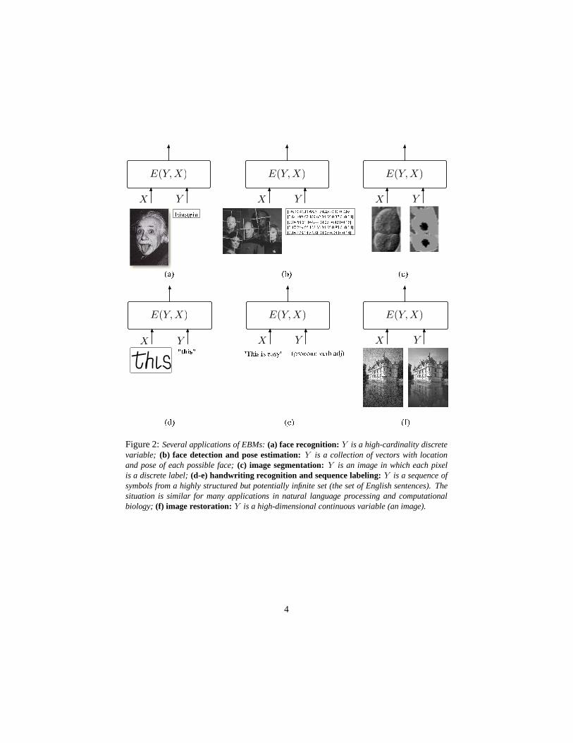
( d ) ( e ) ( f )Figure 2:Several applications of EBMs:(a) face recognition:Y is a high-cardinality discretevariable; (b) face detection and pose estimation:Y is a collection of vectors with locationand pose of each possible face;(c) image segmentation:Y is an image in which each pixelis a discrete label;(d-e) handwriting recognition and sequence labeling:Y is a sequence ofsymbols from a highly structured but potentially infinite set (the set of English sentences). Thesituation is similar for many applications in natural language processing and computationalbiology; (f) image restoration: Y is a high-dimensional continuous variable (an image).

4

In general, however, picking the bestY may not be simple. Figure 2 depicts sev-eral situations in whichY may be too large to make exhaustive search practical. InFigure 2(a), the model is used to recognize a face. In this case, the setY is discreteand finite, but its cardinality may be tens of thousands [Chopra et al., 2005]. In Fig-ure 2(b), the model is used to find the faces in an image and estimate their poses. ThesetY contains a binary variable for each location indicating whether a face is presentat that location, and a set of continuous variables representing the size and orienta-tion of the face [Osadchy et al., 2005]. In Figure 2(c), the model is used to segmenta biological image: each pixel must be classified into one of five categories (cell nu-cleus, nuclear membrane, cytoplasm, cell membrane, external medium). In this case,Y contains all theconsistentlabel images, i.e. the ones for which the nuclear mem-branes are encircling the nuclei, the nuclei and cytoplasm are inside the cells walls,etc. The set is discrete, but intractably large. More importantly, members of the setmust satisfy complicated consistency constraints [Ning etal., 2005]. In Figure 2(d),the model is used to recognize a handwritten sentence. HereY contains all possiblesentences of the English language, which is a discrete but infinite set of sequences ofsymbols [LeCun et al., 1998a]. In Figure 2(f), the model is used to restore an image(by cleaning the noise, enhancing the resolution, or removing scratches). The setYcontains all possible images (all possible pixel combinations). It is a continuous andhigh-dimensional set.

For each of the above situations, a specific strategy, calledtheinference procedure,must be employed to find theY that minimizesE(Y, X). In many real situations, theinference procedure will produce an approximate result, which may or may not be theglobal minimum ofE(Y, X) for a givenX . In fact, there may be situations whereE(Y, X) has several equivalent minima. The best inference procedure to use oftendepends on the internal structure of the model. For example,if Y is continuous andE(Y, X) is smooth and well-behaved with respect toY , one may use a gradient-basedoptimization algorithm. IfY is a collection of discrete variables and the energy func-tion can be expressed as afactor graph, i.e. a sum of energy functions (factors) thatdepend on different subsets of variables, efficient inference procedures for factor graphscan be used (see Section 6) [Kschischang et al., 2001, MacKay, 2003]. A popular ex-ample of such a procedure is themin-sumalgorithm. When each element ofY can berepresented as a path in a weighted directed acyclic graph, then the energy for a partic-ularY is the sum of values on the edges and nodes along a particular path. In this case,the bestY can be found efficiently using dynamic programming (e.g withthe Viterbialgorithm orA∗). This situation often occurs in sequence labeling problems such asspeech recognition, handwriting recognition, natural language processing, and biolog-ical sequence analysis (e.g. gene finding, protein folding prediction, etc). Differentsituations may call for the use of other optimization procedures, including continuousoptimization methods such as linear programming, quadratic programming, non-linearoptimization methods, or discrete optimization methods such as simulated annealing,graph cuts, or graph matching. In many cases, exact optimization is impractical, andone must resort to approximate methods, including methods that use surrogate energyfunctions (such as variational methods).

5

1.2 What Questions Can a Model Answer?

In the preceding discussion, we have implied that the question to be answered by themodel is “What is theY that is most compatible with thisX?”, a situation that occursin prediction, classificationor decision-makingtasks. However, a model may be usedto answer questions of several types:

1. Prediction, classification, and decision-making: “Which value ofY is most com-patible with thisX?’ This situation occurs when the model is used to make harddecisions or to produce an action. For example, if the model is used to drive arobot and avoid obstacles, it must produce a single best decision such as “steerleft”, “steer right”, or “go straight”.

2. Ranking: “Is Y1 or Y2 more compatible with thisX?” This is a more complextask than classification because the system must be trained to produce a completeranking of all the answers, instead of merely producing the best one. This situ-ation occurs in many data mining applications where the model is used to selectmultiple samples that best satisfy a given criterion.

3. Detection: “Is this value ofY compatible withX?” Typically, detection tasks,such as detecting faces in images, are performed by comparing the energy of afacelabel with a threshold. Since the threshold is generally unknown when thesystem is built, the system must be trained to produce energyvalues that increaseas the image looks less like a face.

4. Conditional density estimation: “What is the conditional probability distributionoverY givenX?” This case occurs when the output of the system is not useddirectly to produce actions, but is given to a human decisionmaker or is fed tothe input of another, separately built system.

We often think ofX as a high-dimensional variable (e.g. an image) andY as adiscrete variable (e.g. a label), but the converse case is also common. This occurswhen the model is used for such applications as image restoration, computer graphics,speech and language production, etc. The most complex case is when bothX andYare high-dimensional.

1.3 Decision Making versus Probabilistic Modeling

For decision-making tasks, such as steering a robot, it is merely necessary that the sys-tem give the lowest energy to the correct answer. The energies of other answers areirrelevant, as long as they are larger. However, the output of a system must sometimesbe combined with that of another system, or fed to the input ofanother system (or to ahuman decision maker). Because energies are uncalibrated (i.e. measured in arbitraryunits), combining two, separately trained energy-based models is not straightforward:there is noa priori guarantee that their energy scales are commensurate. Calibratingenergies so as to permit such combinations can be done in a number of ways. However,the onlyconsistentway involves turning the collection of energies for all possible out-puts into a normalized probability distribution. The simplest and most common method

6

for turning a collection of arbitrary energies into a collection of numbers between 0 and1 whose sum (or integral) is 1 is through theGibbs distribution:

P (Y |X) =e−βE(Y,X)

∫

y∈Ye−βE(y,X)

, (2)

whereβ is an arbitrary positive constant akin to an inverse temperature, and the denom-inator is called thepartition function(by analogy with similar concepts in statisticalphysics). The choice of the Gibbs distribution may seem arbitrary, but other proba-bility distributions can be obtained (or approximated) through a suitable re-definitionof the energy function. Whether the numbers obtained this way are good probabilityestimates does not depend on how energies are turned into probabilities, but on howE(Y, X) is estimated from data.

It should be noted that the above transformation of energiesinto probabilities isonly possible if the integral

∫

y∈Ye−βE(y,X) converges. This somewhat restricts the

energy functions and domainsY that can be used. More importantly, there are manypractical situations where computing the partition function is intractable (e.g. whenY has high cardinality), or outright impossible (e.g. whenY is a high dimensionalvariable and the integral has no analytical solution). Hence probabilistic modelingcomes with a high price, and should be avoided when the application does not requireit.

2 Energy-Based Training: Architecture and Loss Func-tion

Training an EBM consists in finding an energy function that produces the bestY foranyX . The search for the best energy function is performed withina family of energyfunctionsE indexed by a parameterW

E = {E(W, Y, X) : W ∈ W}. (3)

Thearchitectureof the EBM is the internal structure of the parameterized energy func-tion E(W, Y, X). At this point, we put no particular restriction on the nature of X ,Y , W , andE . WhenX andY are real vectors,E could be as simple as a linear com-bination of basis functions (as in the case of kernel methods), or a set of neural netarchitectures and weight values. Section gives examples ofsimple architectures forcommon applications to classification and regression. WhenX andY are variable-sizeimages, sequences of symbols or vectors, or more complex structured objects,E mayrepresent a considerably richer class of functions. Sections 4, 6 and 7 discuss severalexamples of such architectures. One advantage of the energy-based approach is that itputs very little restrictions on the nature ofE .

To train the model for prediction, classification, or decision-making, we are givena set of training samplesS = {(X i, Y i) : i = 1 . . . P}, whereX i is the input forthe i-th training sample, andY i is the corresponding desired answer. In order to findthe best energy function in the familyE , we need a way to assess the quality of any

7

particular energy function, based solely on two elements: the training set, and our priorknowledge about the task. This quality measure is called theloss functional(i.e. afunction of function) and denotedL(E,S). For simplicity, we often denote itL(W,S)and simply call it theloss function. The learning problem is simply to find theW thatminimizes the loss:

W ∗ = minW∈W

L(W,S). (4)

For most cases, the loss functional is defined as follows:

L(E,S) =1

P

P∑

i=1

L(Y i, E(W,Y, X i)) + R(W ). (5)

It is an average taken over the training set of aper-sample loss functional, denotedL(Y i, E(W,Y, X i)), which depends on the desired answerY i and on the energiesobtained by keeping the input sample fixed and varying the answer Y . Thus, for eachsample, we evaluate a “slice” of the energy surface. The termR(W ) is theregularizer,and can be used to embed our prior knowledge about which energy functions in ourfamily are preferable to others (in the absence of training data). With this definition,the loss is invariant under permutations of the training samples and under multiplerepetitions of the training set.

Naturally, the ultimate purpose of learning is to produce a model that will givegood answers for new input samples that are not seen during training. We can relyon general results from statistical learning theory which guarantee that, under simpleinterchangeability conditions on the samples and general conditions on the family ofenergy functions (finite VC dimension), the deviation between the value of the lossafter minimization on the training set, and the loss on a large, separate set of testsamples is bounded by a quantity that converges to zero as thesize of training setincreases [Vapnik, 1995].

2.1 Designing a Loss Functional

Intuitively, the per-sample loss functional should be designed in such a way that itassigns a low loss towell-behavedenergy functions: energy functions that give thelowest energy to the correct answer and higher energy to all other (incorrect) answers.Conversely, energy functions that do not assign the lowest energy to the correct answerswould have a high loss. Characterizing the appropriatenessof loss functions (the onesthat select the best energy functions) is further discussedin following sections.

Considering only the task of training a model to answer questions of type 1 (pre-diction, classification and decision-making), the main intuition of the energy-based ap-proach is as follows. Training an EBM consists in shaping theenergy function, so thatfor any givenX , the inference algorithm will produce the desired value forY . Sincethe inference algorithm selects theY with the lowest energy, the learning proceduremust shape the energy surface so that the desired value ofY has lower energy than allother (undesired) values. Figures 3 and 4 show examples of energy as a function ofYfor a given input sampleX i in cases whereY is a discrete variable and a continuousscalar variable. We note three types of answers:

8

H u m a nA n i m a lA i r p l a n eC a rT r u c kE(Y, X)

A f t e rt r a i n i n gH u m a nA n i m a lA i r p l a n eC a rT r u c kE(Y, X)

Figure 3: How training affects the energies of the possible answers inthe discrete case: theenergy of the correct answer is decreased, and the energies of incorrect answers are increased,particularly if they are lower than that of the correct answer.

A n s w e r Yi

Yi

p u l l u pp u s h d o w n(Y )

E(W

,·,X

i)

A n s w e r Yi

Yi

(Y )

E(W

,·,X

i)A f t e rt r a i n i n g

Figure 4:The effect of training on the energy surface as a function of the answerY in the con-tinuous case. After training, the energy of the correct answer Y i is lower than that of incorrectanswers.

9

• Y i: the correct answer

• Y ∗i: the answer produced by the model, i.e. the answer with the lowest energy.

• Y i: the most offending incorrect answer, i.e. the answer that has the lowestenergy among all the incorrect answers. To define this answerin the continuouscase, we can simply view all answers within a distanceǫ of Y i as correct, and allanswers beyond that distance as incorrect.

With a properly designed loss function, the learning process should have the effectof “pushing down” onE(W, Y i, X i), and “pulling up” on the incorrect energies, par-ticularly onE(W, Y i, X i). Different loss functions do this in different ways. Section 5gives sufficient conditions that the loss function must satisfy in order to be guaranteedto shape the energy surface correctly. We show that some widely used loss functionsdo not satisfy the conditions, while others do.

To summarize: given a training setS, building and training an energy-based modelinvolves designing four components:

1. The architecture: the internal structure ofE(W, Y, X).

2. The inference algorithm: the method for finding a value ofY that minimizesE(W, Y, X) for any givenX .

3. The loss function: L(W,S) measures the quality of an energy function using thetraining set.

4. The learning algorithm: the method for finding aW that minimizes the lossfunctional over the family of energy functionsE , given the training set.

Properly designing the architecture and the loss function is critical. Any prior knowl-edge we may have about the task at hand is embedded into the architecture and intothe loss function (particularly the regularizer). Unfortunately, not all combinations ofarchitectures and loss functions are allowed. With some combinations, minimizing theloss will not make the model produce the best answers. Choosing the combinations ofarchitecture and loss functions that can learn effectivelyand efficiently is critical to theenergy-based approach, and thus is a central theme of this tutorial.

2.2 Examples of Loss Functions

We now describe a number of standard loss functions that havebeen proposed and usedin the machine learning literature. We shall discuss them and classify them as “good”or “bad” in an energy-based setting. For the time being, we set aside the regularizationterm, and concentrate on the data-dependent part of the lossfunction.

2.2.1 Energy Loss

The simplest and the most straightforward of all the loss functions is the energy loss.For a training sample(X i, Y i), the per-sample loss is defined simply as:

Lenergy(Y i, E(W,Y, X i)) = E(W, Y i, X i). (6)

10

−4 −3 −2 −1 0 10

0.5

1

1.5

2

2.5

3

EI − E

C

Loss

: L−2 −1.5 −1 −0.5 0 0.5 1 1.50

0.2

0.4

0.6

0.8

1

1.2

1.4

1.6

1.8

EI − E

C

Loss

: L

0 0.5 1 1.5 2 2.5 3 3.50

2

4

6

8

10

12

14

Energy: EC

/ EI

Loss

: L

Figure 5:The hinge loss (left) and log loss (center) penalizeE(W, Y i, Xi)−E(W, Y i, Xi) lin-early and logarithmically, respectively. The square-square loss (right) separately penalizes largevalues ofE(W,Y i, Xi) (solid line) and small values ofE(W, Y i, Xi) (dashed line) quadrati-cally.

This loss function, although very popular for things like regression and neural networktraining, cannot be used to train most architectures: whilethis loss will push downon the energy of the desired answer, it will not pull up on any other energy. Withsome architectures, this can lead to acollapsed solutionin which the energy is con-stant and equal to zero. The energy loss will only work with architectures that aredesigned in such a way that pushing down onE(W, Y i, X i) will automatically makethe energies of the other answers larger. A simple example ofsuch an architecture isE(W, Y i, X i) = ||Y i − G(W, X i)||2, which corresponds to regression with mean-squared error withG being the regression function.

2.2.2 Generalized Perceptron Loss

The generalized perceptron loss for a training sample(X i, Y i) is defined as

Lperceptron(Y i, E(W,Y, X i)) = E(W, Y i, X i)− minY ∈Y

E(W, Y, X i). (7)

This loss is always positive, since the second term is a lowerbound on the first term.Minimizing this loss has the effect of pushing down onE(W, Y i, X i), while pullingup on the energy of the answer produced by the model.

While the perceptron loss has been widely used in many settings, including formodels with structured outputs such as handwriting recognition [LeCun et al., 1998a]and parts of speech tagging [Collins, 2002], it has a major deficiency: there is no mech-anism for creating an energy gap between the correct answer and the incorrect ones.Hence, as with the energy loss, the perceptron loss may produce flat (or almost flat)energy surfaces if the architecture allows it. Consequently, a meaningful, uncollapsedresult is only guaranteed with this loss if a model is used that cannot produce a flatenergy surface. For other models, one cannot guarantee anything.

2.2.3 Generalized Margin Losses

Several loss functions can be described asmarginlosses; the hinge loss, log loss, LVQ2loss, minimum classification error loss, square-square loss, and square-exponential lossall use some form of margin to create an energy gap between thecorrect answer and the

11

incorrect answers. Before discussing the generalized margin loss we give the followingdefinitions.

Definition 1 Let Y be a discrete variable. Then for a training sample(X i, Y i), themost offending incorrect answer Y i is the answer that has the lowest energy amongall answers that are incorrect:

Y i = argminY ∈YandY 6=Y iE(W, Y, X i). (8)

If Y is a continuous variable then the definition of the most offending incorrect answercan be defined in a number of ways. The simplest definition is asfollows.

Definition 2 LetY be a continuous variable. Then for a training sample(X i, Y i), themost offending incorrect answer Y i is the answer that has the lowest energy amongall answers that are at leastǫ away from the correct answer:

Y i = argminY ∈Y,‖Y −Y i‖>ǫE(W, Y, X i). (9)

The generalized margin loss is a more robust version of the generalized perceptronloss. It directly uses the energy of the most offending incorrect answer in the contrastiveterm:

Lmargin(W, Y i, X i) = Qm

(

E(W, Y i, X i), E(W, Y i, X i))

. (10)

Herem is a positive parameter called themarginandQm(e1, e2) is a convex functionwhose gradient has a positive dot product with the vector[1,−1] in the region whereE(W, Y i, X i)+m > E(W, Y i, X i). In other words, the loss surface is slanted towardlow values ofE(W, Y i, X i) and high values ofE(W, Y i, X i) whereverE(W, Y i, X i)is not smaller thanE(W, Y i, X i) by at leastm. Two special cases of the generalizedmargin loss are given below:

Hinge Loss: A particularly popular example of generalized margin lossisthe hinge loss, which is used in combination with linearly parameterized en-ergies and a quadratic regularizer in support vector machines, support vectorMarkov models [Altun and Hofmann, 2003], and maximum-margin Markov net-works [Taskar et al., 2003]:

Lhinge(W, Y i, X i) = max(

0, m + E(W, Y i, X i)− E(W, Y i, X i))

, (11)

wherem is the positive margin. The shape of this loss function is given in Figure 5. Thedifference between the energies of the correct answer and the most offending incorrectanswer is penalized linearly when larger than−m. The hinge loss only depends onenergy differences, hence individual energies are not constrained to take any particularvalue.

Log Loss: a common variation of the hinge loss is thelog loss, which can be seenas a “soft” version of the hinge loss with an infinite margin (see Figure 5, center):

Llog(W, Y i, X i) = log(

1 + eE(W,Y i,Xi)−E(W,Y i,Xi))

. (12)

LVQ2 Loss: One of the very first proposals for discriminatively train-ing sequence labeling systems (particularly speech recognition systems)

12

is a version of Kohonen’s LVQ2 loss. This loss has been advocatedby Driancourt and Bottou since the early 90’s [Driancourt etal., 1991a,Driancourt and Gallinari, 1992b, Driancourt and Gallinari, 1992a, Driancourt, 1994,McDermott, 1997, McDermott and Katagiri, 1992]:

Llvq2(W, Y i, X i) = min

(

1, max

(

0,E(W, Y i, X i)− E(W, Y i, X i)

δE(W, Y i, X i)

))

, (13)

whereδ is a positive parameter. LVQ2 is a zero-margin loss, but it has the peculiarity ofsaturating the ratio betweenE(W, Y i, X i) andE(W, Y i, X i) to 1 + δ. This mitigatesthe effect of outliers by making them contribute a nominal cost M to the total loss.This loss function is a continuous approximation of the number of classification errors.Unlike generalized margin losses, the LVQ2 loss is non-convex in E(W, Y i, X i) andE(W, Y i, X i).

MCE Loss: The Minimum Classification Error loss was originally proposed byJuang et al. in the context of discriminative training for speech recognition sys-tems [Juang et al., 1997]. The motivation was to build a loss function that also ap-proximately counts the number of classification errors, while being smooth and differ-entiable. The number of classification errors can be writtenas:

θ(

E(W, Y i, X i)− E(W, Y i, X i))

, (14)

whereθ is the step function (equal to zero for negative arguments, and 1 for positivearguments). However, this function is not differentiable,and therefore very difficult tooptimize. The MCE Loss “softens” it with a sigmoid:

Lmce(W, Y i, X i) = σ(

E(W, Y i, X i)− E(W, Y i, X i))

, (15)

whereσ is the logistic functionσ(x) = (1 + e−x)−1. As with the LVQ2 loss, the satu-ration ensures that mistakes contribute a nominal cost to the overall loss. Although theMCE loss does not have an explicit margin, it does create a gapbetweenE(W, Y i, X i)andE(W, Y i, X i). The MCE loss is non-convex.

Square-Square Loss: Unlike the hinge loss, the square-square loss treatsthe energy of the correct answer and the most offending answer sepa-rately [LeCun and Huang, 2005, Hadsell et al., 2006]:

Lsq−sq(W, Y i, X i) = E(W, Y i, X i)2 +(

max(0, m− E(W, Y i, X i)))2

. (16)

Large values ofE(W, Y i, X i) and small values ofE(W, Y i, X i) below the marginmare both penalized quadratically (see Figure 5). Unlike themargin loss, the square-square loss “pins down” the correct answer energy at zero and“pins down” the incor-rect answer energies abovem. Therefore, it is only suitable for energy functions thatare bounded below by zero, notably in architectures whose output module measuressome sort of distance.

Square-Exponential [LeCun and Huang, 2005, Chopra et al., 2005,Osadchy et al., 2005]: Thesquare-exponentialloss is similar to thesquare-squareloss. It only differs in the contrastive term: instead of a quadratic term it has theexponential of the negative energy of the most offending incorrect answer:

Lsq−exp(W, Y i, X i) = E(W, Y i, X i)2 + γe−E(W,Y i,Xi), (17)

13

whereγ is a positive constant. Unlike the square-square loss, thisloss has an infinitemargin and pushes the energy of the incorrect answers to infinity with exponentiallydecreasing force.

2.2.4 Negative Log-Likelihood Loss

The motivation for the negative log-likelihood loss comes from probabilistic modeling.It is defined as:

Lnll(W, Y i, X i) = E(W, Y i, X i) + Fβ(W,Y, X i). (18)

WhereF is thefree energyof the ensemble{E(W, y, X i), y ∈ Y}:

Fβ(W,Y, X i) =1

βlog

(∫

y∈Y

exp(

−βE(W, y, X i))

)

. (19)

whereβ is a positive constant akin to an inverse temperature. This loss can only beused if the exponential of the negative energy is integrableoverY, which may not bethe case for some choices of energy function orY.

The form of the negative log-likelihood loss stems from a probabilistic formulationof the learning problem in terms of the maximum conditional probability principle.Given the training setS, we must find the value of the parameter that maximizes theconditional probability of all the answers given all the inputs in the training set. Assum-ing that the samples are independent, and denoting byP (Y i|X i, W ) the conditionalprobability ofY i givenX i that is produced by our model with parameterW , the condi-tional probability of the training set under the model is a simple product over samples:

P (Y 1, . . . , Y P |X1, . . . , XP , W ) =

P∏

i=1

P (Y i|X i, W ). (20)

Applying the maximum likelihood estimation principle, we seek the value ofW thatmaximizes the above product, or the one that minimizes the negativelog of the aboveproduct:

− log

P∏

i=1

P (Y i|X i, W ) =

P∑

i=1

− log P (Y i|X i, W ). (21)

Using the Gibbs distribution (Equation 2), we get:

− log

P∏

i=1

P (Y i|X i, W ) =

P∑

i=1

βE(W, Y i, X i) + log

∫

y∈Y

e−βE(W,y,Xi). (22)

The final form of the negative log-likelihood loss is obtained by dividing the aboveexpression byP andβ (which has no effect on the position of the minimum):

Lnll(W,S) =1

P

P∑

i=1

(

E(W, Y i, X i) +1

βlog

∫

y∈Y

e−βE(W,y,Xi)

)

. (23)

14

While many of the previous loss functions involved onlyE(W, Y i, X i) in their con-trastive term, the negative log-likelihood loss combines all the energies for all val-ues ofY in its contrastive termFβ(W,Y, X i). This term can be interpreted as theHelmholtz free energy (log partition function) of the ensemble of systems with ener-giesE(W, Y, X i), Y ∈ Y. This contrastive term causes the energies of all the answersto be pulled up. The energy of the correct answer is also pulled up, but not as hard as itis pushed down by the first term. This can be seen in the expression of the gradient fora single sample:

∂Lnll(W, Y i, X i)

∂W=

∂E(W, Y i, X i)

∂W−

∫

Y ∈Y

∂E(W, Y, X i)

∂WP (Y |X i, W ), (24)

whereP (Y |X i, W ) is obtained through the Gibbs distribution:

P (Y |X i, W ) =e−βE(W,Y,Xi)

∫

y∈Y e−βE(W,y,Xi). (25)

Hence, the contrastive term pulls up on the energy of each answer with a force propor-tional to the likelihood of that answer under the model. Unfortunately, there are manyinteresting models for which computing the integral overY is intractable. Evaluatingthis integral is a major topic of research. Considerable efforts have been devoted to ap-proximation methods, including clever organization of thecalculations, Monte-Carlosampling methods, and variational methods. While these methods have been devised asapproximate ways of minimizing the NLL loss, they can be viewed in the energy-basedframework as different strategies for choosing theY ’s whose energies will be pulledup.

Interestingly, the NLL loss reduces to the generalized perceptron loss whenβ →∞(zero temperature), and reduces to the log loss (Eq. 12) whenY has two elements (e.g.binary classification).

The NLL loss has been used extensively by many authors under variousnames. In the neural network classification literature, it is known as thecross-entropy loss[Solla et al., 1988]. It was also used by Bengio et al. to trainanenergy-based language model [Bengio et al., 2003]. It has been widely used un-der the namemaximum mutual information estimationfor discriminatively train-ing speech recognition systems since the late 80’s, including hidden Markovmodels with mixtures of Gaussians [Bahl et al., 1986], and HMM-neural net hy-brids [Bengio et al., 1990, Bengio et al., 1992, Haffner, 1993, Bengio, 1996]. It hasalso been used extensively for global discriminative training of handwriting recog-nition systems that integrate neural nets and hidden Markovmodels under thenamesmaximum mutual information[Bengio et al., 1993, LeCun and Bengio, 1994,Bengio et al., 1995, LeCun et al., 1997, Bottou et al., 1997] and discriminative for-ward training [LeCun et al., 1998a]. Finally, it is the loss function of choice for train-ing other probabilistic discriminative sequence labelingmodels such as input/outputHMM [Bengio and Frasconi, 1996], conditional random fields [Lafferty et al., 2001],and discriminative random fields [Kumar and Hebert, 2004].

Minimum Empirical Error Loss : Some authors have argued that the negative loglikelihood loss puts too much emphasis on mistakes: Eq. 20 isa product whose value

15

is dominated by its smallest term. Hence, Ljolje et al. [Ljolje et al., 1990] proposedtheminimum empirical error loss, which combines the conditional probabilities of thesamples additively instead of multiplicatively:

Lmee(W, Y i, X i) = 1− P (Y i|X i, W ). (26)

Substituting Equation 2 we get:

Lmee(W, Y i, X i) = 1−e−βE(W,Y i,Xi)

∫

y∈Ye−βE(W,y,Xi)

. (27)

As with the MCE loss and the LVQ2 loss, the MEE loss saturates the contributionof any single error. This makes the system more robust to label noise and outliers,which is of particular importance to such applications suchas speech recognition, butit makes the loss non-convex. As with the NLL loss, MEE requires evaluating thepartition function.

3 Simple Architectures

To substantiate the ideas presented thus far, this section demonstrates how simple mod-els of classification and regression can be formulated as energy-based models. This setsthe stage for the discussion of good and bad loss functions, as well as for the discussionof advanced architectures for structured prediction.

D(GW (X), Y )

X Y X Y

−Y · GW (X)

X Y

g0 g1 g2

E(W,Y, X)E(W,Y, X)

GW (X) GW (X) GW (X)

E(W,Y, X) =

3∑

k=1

δ(Y − k)gk

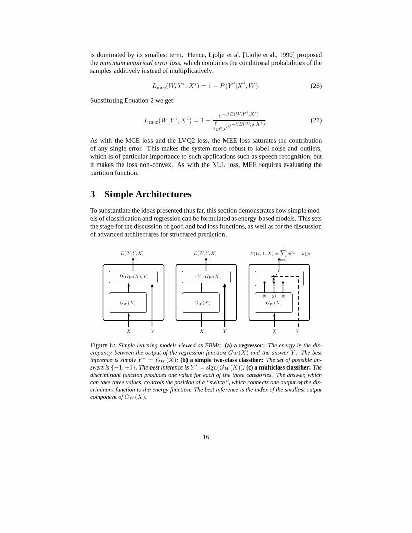
Figure 6: Simple learning models viewed as EBMs:(a) a regressor: The energy is the dis-crepancy between the output of the regression functionGW (X) and the answerY . The bestinference is simplyY ∗ = GW (X); (b) a simple two-class classifier:The set of possible an-swers is{−1, +1}. The best inference isY ∗ = sign(GW (X)); (c) a multiclass classifier:Thediscriminant function produces one value for each of the three categories. The answer, whichcan take three values, controls the position of a “switch”, which connects one output of the dis-criminant function to the energy function. The best inference is the index of the smallest outputcomponent ofGW (X).

16

3.1 Regression

Figure 6(a) shows a simple architecture for regression or function approximation. Theenergy function is the squared error between the output of a regression functionGW (X)and the variable to be predictedY , which may be a scalar or a vector:

E(W, Y, X) =1

2||GW (X)− Y ||2. (28)

The inference problem is trivial: the value ofY that minimizesE is equal toGW (X).The minimum energy is always equal to zero. When used with this architecture, theenergy loss, perceptron loss, and negative log-likelihoodloss are all equivalent becausethe contrastive term of the perceptron loss is zero, and thatof the NLL loss is constant(it is a Gaussian integral with a constant variance):

Lenergy(W,S) =1

P

P∑

i=1

E(W, Y i, X i) =1

2P

P∑

i=1

||GW (X i)− Y i||2. (29)

This corresponds to standard regression with mean-squarederror.A popular form of regression occurs whenG is a linear function of the parameters:

GW (X) =

N∑

k=1

wkφk(X) = WT Φ(X). (30)

Theφk(X) are a set ofN features, andwk are the components of anN -dimensionalparameter vectorW . For concision, we use the vector notationWT Φ(X), whereWT

denotes the transpose ofW , andΦ(X) denotes the vector formed by eachφk(X). Withthis linear parameterization, training with the energy loss reduces to an easily solvableleast-squares minimization problem, which is convex:

W ∗ = argminW

[

1

2P

P∑

i=1

||WT Φ(X i)− Y i||2

]

. (31)

In simple models, the feature functions are hand-crafted bythe designer, or separatelytrained from unlabeled data. In the dual form of kernel methods, they are defined asφk(X) = K(X, Xk), k = 1 . . . P , whereK is the kernel function. In more complexmodels such as multilayer neural networks and others, theφ’s may themselves be pa-rameterized and subject to learning, in which case the regression function is no longera linear function of the parameters and hence the loss function may not be convex inthe parameters.

3.2 Two-Class Classifier

Figure 6(b) shows a simple two-class classifier architecture. The variable to be pre-dicted is binary:Y = {−1, +1}. The energy function can be defined as:

E(W, Y, X) = −Y GW (X), (32)

17

whereGW (X) is a scalar-valueddiscriminant functionparameterized byW . Inferenceis trivial:

Y ∗ = argminY ∈{−1,1} − Y GW (X) = sign(GW (X)). (33)

Learning can be done using a number of different loss functions, which include theperceptron loss, hinge loss, and negative log-likelihood loss. Substituting Equations 32and 33 into the perceptron loss (Eq. 7), we get:

Lperceptron(W,S) =1

P

P∑

i=1

(

sign(GW (X i))− Y i)

GW (X i). (34)

The stochastic gradient descent update rule to minimize this loss is:

W ←W + η(

Y i − sign(GW (X i)) ∂GW (X i)

∂W, (35)

whereη is a positive step size. If we chooseGW (X) in the family of linear models,the energy function becomesE(W, Y, X) = −Y WT Φ(X) and the perceptron lossbecomes:

Lperceptron(W,S) =1

P

P∑

i=1

(

sign(WT Φ(X i))− Y i)

WT Φ(X i), (36)

and the stochastic gradient descent update rule becomes thefamiliar perceptron learn-ing rule:W ←W + η

(

Y i − sign(WT Φ(X i)))

Φ(X i).The hinge loss (Eq. 11) with the two-class classifier energy (Eq. 32) yields:

Lhinge(W,S) =1

P

P∑

i=1

max(0, m + 2Y iGW (X i)). (37)

Using this loss withGW (X) = WT X and a regularizer of the form||W ||2 gives thefamiliar linear support vector machine.

The negative log-likelihood loss (Eq. 23) with Equation 32 yields:

Lnll(W,S) =1

P

P∑

i=1

[

−Y iGW (X i) + log(

eY iGW (Xi) + e−Y iGW (Xi))]

. (38)

Using the fact thatY = {−1, +1}, we obtain:

Lnll(W,S) =1

P

P∑

i=1

log(

1 + e−2Y iGW (Xi))

, (39)

which is equivalent to the log loss (Eq. 12). Using a linear model as described above,the loss function becomes:

Lnll(W,S) =1

P

P∑

i=1

log(

1 + e−2Y iW T Φ(Xi))

. (40)

This particular combination of architecture and loss is thefamiliar logistic regressionmethod.

18

3.3 Multiclass Classifier

Figure 6(c) shows an example of architecture for multiclassclassification for 3 classes.A discriminant functionGW (X) produces an output vector[g1, g2, . . . , gC ] with onecomponent for each of theC categories. Each componentgj can be interpreted asa “penalty” for assigningX to the jth category. A discrete switch module selectswhich of the components is connected to the output energy. The position of the switchis controlled by the discrete variableY ∈ {1, 2, . . . , C}, which is interpreted as thecategory. The output energy is equal toE(W, Y, X) =

∑C

j=1 δ(Y − j)gj , whereδ(Y − j) is the Kronecker delta function:δ(u) = 1 for u = 0; δ(u) = 0 otherwise.Inference consists in settingY to the index of the smallest component ofGW (X).

The perceptron loss, hinge loss, and negative log-likelihood loss can be directlytranslated to the multiclass case.

3.4 Implicit Regression

E(W,Y, X)

X Y

GW (X)G1W1(X) HW2

(X)

||G1W1(X)−G2W2

(Y )||1

G2W2(Y )

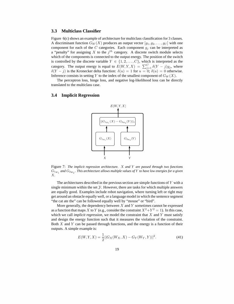
Figure 7: The implicit regression architecture.X and Y are passed through two functionsG1W1

andG2W2. This architecture allows multiple values ofY to have low energies for a given

X.

The architectures described in the previous section are simple functions ofY with asingle minimum within the setY. However, there are tasks for which multiple answersare equally good. Examples include robot navigation, whereturning left or right mayget around an obstacle equally well, or a language model in which the sentence segment“the cat ate the” can be followed equally well by “mouse” or “bird”.

More generally, the dependency betweenX andY sometimes cannot be expressedas a function that mapsX toY (e.g., consider the constraintX2+Y 2 = 1). In this case,which we callimplicit regression, we model the constraint thatX andY must satisfyand design the energy function such that it measures the violation of the constraint.Both X andY can be passed through functions, and the energy is a functionof theiroutputs. A simple example is:

E(W, Y, X) =1

2||GX(WX , X)−GY (WY , Y )||2. (41)

19

For some problems, the functionGX must be different from the functionGY . Inother cases,GX andGY must be instances of the same functionG. An interestingexample is theSiamesearchitecture [Bromley et al., 1993]: variablesX1 andX2 arepassed through two instances of a functionGW . A binary labelY determines the con-straint onGW (X1) andGW (X2): if Y = 0, GW (X1) andGW (X2) should be equal,and if Y = 1, GW (X1) andGW (X2) should be different. In this way, the regres-sion onX1 andX2 is implicitly learned through the constraintY rather than explicitlylearned through supervision. Siamese architectures are used to learn similarity metricswith labeled examples. When two input samplesX1 andX2 are known to be similar(e.g. two pictures of the same person),Y = 0; when they are different,Y = 1.

Siamese architectures were originally designed for signature verification [Bromley et al., 1993].More recently they have been used with the square-exponential loss (Eq. 17) to learn asimilarity metric with application to face recognition [Chopra et al., 2005]. They havealso been used with the square-square loss (Eq. 16) for unsupervised learning of mani-folds [Hadsell et al., 2006].

In other applications, a single non-linear function combinesX andY . An exampleof such architecture is the trainable language model of Bengio et al [Bengio et al., 2003].Under this model, the inputX is a sequence of a several successive words in a text, andthe answerY is the the next word in the text. Since many different words can followa particular word sequence, the architecture must allow multiple values ofY to havelow energy. The authors used a multilayer neural net as the functionG(W, X, Y ), andchose to train it with the negative log-likelihood loss. Because of the high cardinal-ity of Y (equal to the size of the English dictionary), they had to useapproximations(importance sampling) and had to train the system on a cluster machine.

The current section often referred to architectures in which the energy was linear orquadratic inW , and the loss function was convex inW , but it is important to keep inmind that much of the discussion applies equally well to morecomplex architectures,as we will see later.

4 Latent Variable Architectures

Energy minimization is a convenient way to represent the general process of reasoningand inference. In the usual scenario, the energy is minimized with respect to the vari-ables to be predictedY , given the observed variablesX . During training, the correctvalue ofY is given for each training sample. However there are numerous applicationswhere it is convenient to use energy functions that depend ona set of hidden variablesZ whose correct value is never (or rarely) given to us, even during training. For ex-ample, we could imagine training the face detection system depicted in Figure 2(b)with data for which the scale and pose information of the faces is not available. Forthese architectures, the inference process for a given set of variablesX andY involvesminimizing over these unseen variablesZ:

E(Y, X) = minZ∈Z

E(Z, Y, X). (42)

Such hidden variables are calledlatent variables, by analogy with a similar concept inprobabilistic modeling. The fact that the evaluation ofE(Y, X) involves a minimiza-

20

tion overZ does not significantly impact the approach described so far,but the use oflatent variables is so ubiquitous that it deserves special treatment.

In particular, some insight can be gained by viewing the inference process in thepresence of latent variables as a simultaneous minimization overY andZ:

Y ∗ = argminY ∈Y,Z∈ZE(Z, Y, X). (43)

Latent variables can be viewed as intermediate results on the way to finding the bestoutputY . At this point, one could argue that there is no conceptual difference betweentheZ andY variables:Z could simply be folded intoY . The distinction arises duringtraining: we are given the correct value ofY for a number of training samples, but weare never given the correct value ofZ.

Latent variables are very useful in situations where a hidden characteristic of theprocess being modeled can be inferred from observations, but cannot be predicted di-rectly. One such example is in recognition problems. For example, in face recognitionthe gender of a person or the orientation of the face could be alatent variable. Knowingthese values would make the recognition task much easier. Likewise in invariant objectrecognition the pose parameters of the object (location, orientation, scale) or the illumi-nation could be latent variables. They play a crucial role inproblems where segmenta-tion of the sequential data must be performed simultaneously with the recognition task.A good example is speech recognition, in which the segmentation of sentences intowords and words into phonemes must take place simultaneously with recognition, yetthe correct segmentation into phonemes is rarely availableduring training. Similarly, inhandwriting recognition, the segmentation of words into characters should take placesimultaneously with the recognition. The use of latent variables in face recognition isdiscussed in this section, and Section 7.3 describes a latent variable architecture forhandwriting recognition.

4.1 An Example of Latent Variable Architecture

To illustrate the concept of latent variables, we consider the task of face detection,beginning with the simple problem of determining whether a face is present or not ina small image. Imagine that we are provided with a face detecting functionGface(X)which takes a small image window as input and produces a scalar output. It outputsa small value when a human face fills the input image, and a large value if no face ispresent (or if only a piece of a face or a tiny face is present).An energy-based facedetector built around this function is shown in Figure 8(a).The variableY controls theposition of a binary switch (1 = “face”, 0 = “non-face”). The output energy is equalto Gface(X) whenY = 1, and to a fixed threshold valueT whenY = 0:

E(Y, X) = Y Gface(X) + (1− Y )T.

The value ofY that minimizes this energy function is1 (face) if Gface(X) < T and0(non-face) otherwise.

Let us now consider the more complex task ofdetecting and locatinga single facein a large image. We can apply ourGface(X) function to multiple windows in the largeimage, compute which window produces the lowest value ofGface(X), and detect a

21

E(W,Y, X)

X Y

" f a c e " ( = 1 )o r" n o f a c e " ( = 0 )GW (X)

TGface(X)

X Y

" f a c e " ( = 1 )o r" n o f a c e " ( = 0 )GW (X)

T

Z

E(W,Z, Y, X)

p o s i t i o no ff a c eGface(X) Gface(X) Gface(X) Gface(X)

(a) (b)

Figure 8: (a): Architecture of an energy-based face detector. Given an image, it outputs asmall value when the image is filled with a human face, and a high value equal to the thresholdT when there is no face in the image.(b): Architecture of an energy-based face detector thatsimultaneously locates and detects a face in an input image by using the location of the face asa latent variable.

face at that location if the value is lower thanT . This process is implemented bythe energy-based architecture shown in Figure 8(b). The latent “location” variableZselects which of theK copies of theGface function is routed to the output energy. Theenergy function can be written as

E(Z, Y, X) = Y

[

K∑

k=1

δ(Z − k)Gface(Xk)

]

+ (1 − Y )T, (44)

where theXk’s are the image windows. Locating the best-scoring location in the imageconsists in minimizing the energy with respect toY andZ. The resulting value ofYwill indicate whether a face was found, and the resulting value ofZ will indicate thelocation.

4.2 Probabilistic Latent Variables

When the best value of the latent variable for a givenX andY is ambiguous, one mayconsider combining the contributions of the various possible values by marginalizingover the latent variables instead of minimizing with respect to those variables.

When latent variables are present, the joint conditional distribution overY andZ

22

given by the Gibbs distribution is:

P (Z, Y |X) =e−βE(Z,Y,X)

∫

y∈Y, z∈Z e−βE(y,z,X). (45)

Marginalizing overZ gives:

P (Y |X) =

∫

z∈Z e−βE(Z,Y,X)

∫

y∈Y, z∈Ze−βE(y,z,X)

. (46)

Finding the bestY after marginalizing overZ reduces to:

Y ∗ = argminY ∈Y −1

βlog

∫

z∈Z

e−βE(z,Y,X). (47)

This is actually a conventional energy-based inference in which the energy function hasmerely been redefined fromE(Z, Y, X) toF(Z) = − 1

βlog∫

z∈Ze−βE(z,Y,X), which

is thefree energyof the ensemble{E(z, Y, X), z ∈ Z}. The above inference formulaby marginalization reduces to the previous inference formula by minimization whenβ →∞ (zero temperature).

5 Analysis of Loss Functions for Energy-Based Models

This section discusses the conditions that a loss function must satisfy so that its mini-mization will result in a model that produces the correct answers. To give an intuitionof the problem, we first describe simple experiments in whichcertain combinations ofarchitectures and loss functions are used to learn a simple dataset, with varying results.A more formal treatment follows in Section 5.2.

5.1 “Good” and “Bad” Loss Functions

Consider the problem of learning a function that computes the square of a number:Y = f(X), wheref(X) = X2. Though this is a trivial problem for a learningmachine, it is useful for demonstrating the issues involvedin the design of an energyfunction and loss function that work together. For the following experiments, we usea training set of200 samples(X i, Y i) whereY i = X i2, randomly sampled with auniform distribution between−1 and+1.

First, we use the architecture shown in Figure 9(a). The input X is passed througha parametric functionGW , which produces a scalar output. The output is comparedwith the desired answer using the absolute value of the difference (L1 norm):

E(W, Y, X) = ||GW (X)− Y ||1. (48)

Any reasonable parameterized family of functions could be used forGW . For theseexperiments, we chose a two-layer neural network with 1 input unit, 20 hidden units(with sigmoids) and 1 output unit. Figure 10(a) shows the initial shape of the energy

23

E(W,Y, X)

X Y

GW (X)

||GW (X)− Y ||1

GW (X)

E(W,Y, X)

X Y

GW (X)G1W1(X) HW2

(X)

||G1W1(X)−G2W2

(Y )||1

G2W2(Y )

(a) (b)

Figure 9: (a): A simple architecture that can be trained with theenergyloss. (b): An implicitregression architecture whereX andY are passed through functionsG1W1

andG2W2respec-

tively. Training this architecture with the energy loss causes a collapse (a flat energy surface). Aloss function with a contrastive term corrects the problem.

function in the space of the variablesX andY , using a set of random initial parametersW . The dark spheres mark the location of a few training samples.

First, the simple architecture is trained with the energy loss (Eq. 6):

Lenergy(W,S) =1

P

P∑

i=1

E(W, Y i, X i) =1

P

P∑

i=1

||GW (X)− Y ||1. (49)

This corresponds to a classical form of robust regression. The learning process can beviewed as pulling down on the energy surface at the location of the training samples (thespheres in Figure 10), without considering the rest of the points on the energy surface.The energy surface as a function ofY for anyX has the shape of a V with fixed slopes.By changing the functionGW (X), the apex of that V can move around for differentX i. The loss is minimized by placing the apex of the V at the position Y = X2 forany value ofX , and this has the effect of making the energies of all other answerslarger, because the V has a single minimum. Figure 10 shows the shape of the energysurface at fixed intervals during training with simple stochastic gradient descent. Theenergy surface takes the proper shape after a few iterationsthrough the training set.Using more sophisticated loss functions such as the NLL lossor the perceptron losswould produce exactly the same result as the energy loss because, with this simplearchitecture, their contrastive term is constant.

Consider a slightly more complicated architecture, shown in Figure 9(b), to learnthe same dataset. In this architectureX is passed through functionG1W1

andY ispassed through functionG2W2

. For the experiment, both functions were two-layerneural networks with 1 input unit, 10 hidden units and 10 output units. The energy is

24

(a) (b) (c) (d)

Figure 10:The shape of the energy surface at four intervals while training the system in Fig-ure 9(a) with stochastic gradient descent to minimize theenergy loss. TheX axis is the input,and theY axis the output. The energy surface is shown (a) at the start of training, (b) after 10epochs through the training set, (c) after 25 epochs, and (d)after 39 epochs. The energy surfacehas attained the desired shape where the energy around training samples (dark spheres) is lowand energy at all other points is high.

theL1 norm of the difference between their 10-dimensional outputs:

E(W, X, Y ) = ||G1W1(X)−G2W2

(Y )||1, (50)

whereW = [W1W2]. Training this architecture with the energy loss results ina col-lapseof the energy surface. Figure 11 shows the shape of the energysurface duringtraining; the energy surface becomes essentially flat. Whathas happened? The shapeof the energy as a function ofY for a givenX is no longer fixed. With the energy loss,there is no mechanism to preventG1 andG2 from ignoring their inputs and producingidentical output values. This results in the collapsed solution: the energy surface is flatand equal to zero everywhere.

(a) (b) (c) (d)

Figure 11:The shape of the energy surface at four intervals while training the system in Fig-ure 9(b) using the energy loss. Along theX axis is the input variable and along theY axis is theanswer. The shape of the surface (a) at the start of the training, (b) after 3 epochs through thetraining set, (c) after 6 epochs, and (d) after 9 epochs. Clearly the energy is collapsing to a flatsurface.

Now consider the same architecture, but trained with thesquare-squareloss:

L(W, Y i, X i) = E(W, Y i, X i)2 −(

max(0, m− E(W, Y i, X i)))2

. (51)

Herem is a positive margin, andY i is the most offending incorrect answer. The secondterm in the loss explicitly prevents the collapse of the energy by pushing up on points

25

whose energy threatens to go below that of the desired answer. Figure 12 shows theshape of the energy function during training; the surface successfully attains the desiredshape.

(a) (b) (c) (d)

Figure 12:The shape of the energy surface at four intervals while training the system in Fig-ure 9(b) usingsquare-squareloss. Along the x-axis is the variableX and along the y-axis is thevariableY . The shape of the surface at (a) the start of the training, (b)after 15 epochs over thetraining set, (c) after 25 epochs, and (d) after 34 epochs. The energy surface has attained thedesired shape: the energies around the training samples arelow and energies at all other pointsare high.

(a) (b) (c) (d)

Figure 13:The shape of the energy surface at four intervals while training the system in Fig-ure 9(b) using the negative log-likelihood loss. Along theX axis is the input variable and alongtheY axis is the answer. The shape of the surface at (a) the start oftraining, (b) after 3 epochsover the training set, (c) after 6 epochs, and (d) after 11 epochs. The energy surface has quicklyattained the desired shape.

Another loss function that works well with this architecture is thenegative log-likelihood loss:

L(W, Y i, X i) = E(W, Y i, X i) +1

βlog

(∫

y∈Y

e−βE(W,y,Xi)

)

. (52)

The first term pulls down on the energy of the desired answer, while the second termpushes up on all answers, particularly those that have the lowest energy. Note thatthe energy corresponding to the desired answer also appearsin the second term. Theshape of the energy function at various intervals using the negative log-likelihood lossis shown in Figure 13. The learning is much faster than the square-square loss. Theminimum is deeper because, unlike with the square-square loss, the energies of the in-correct answers are pushed up to infinity (although with a decreasing force). However,

26

each iteration of negative log-likelihood loss involves considerably more work becausepushing up every incorrect answer is computationally expensive when no analyticalexpression for the derivative of the second term exists. In this experiment, a simplesampling method was used: the integral is approximated by a sum of 20 points regu-larly spaced between -1 and +1 in theY direction. Each learning iteration thus requirescomputing the gradient of the energy at 20 locations, versus2 locations in the caseof the square-square loss. However, the cost of locating themost offending incorrectanswer must be taken into account for the square-square loss.

An important aspect of the NLL loss is that it is invariant to global shifts of energyvalues, and only depends on differences between the energies of theY s for a givenX .Hence, the desired answer may have different energies for differentX , and may not bezero. This has an important consequence:the quality of an answer cannot be measuredby the energy of that answer without considering the energies of all other answers.

In this section we have seen the results of training four combinations of architec-tures and loss functions. In the first case we used a simple architecture along with asimple energy loss, which was satisfactory. The constraints in the architecture of thesystem automatically lead to the increase in energy of undesired answers while de-creasing the energies of the desired answers. In the second case, a more complicatedarchitecture was used with the simple energy loss and the machine collapsed for lackof a contrastive term in the loss. In the third and the fourth case the same architecturewas used as in the second case but with loss functions containing explicit contrastiveterms. In these cases the machine performed as expected and did not collapse.

5.2 Sufficient Conditions for Good Loss Functions

In the previous section we offered some intuitions about which loss functions are goodand which ones are bad with the help of illustrative experiments. In this section a moreformal treatment of the topic is given. First, a set of sufficient conditions are stated.The energy function and the loss function must satisfy theseconditions in order to beguaranteed to work in an energy-based setting. Then we discuss the quality of the lossfunctions introduced previously from the point of view of these conditions.

5.3 Conditions on the Energy

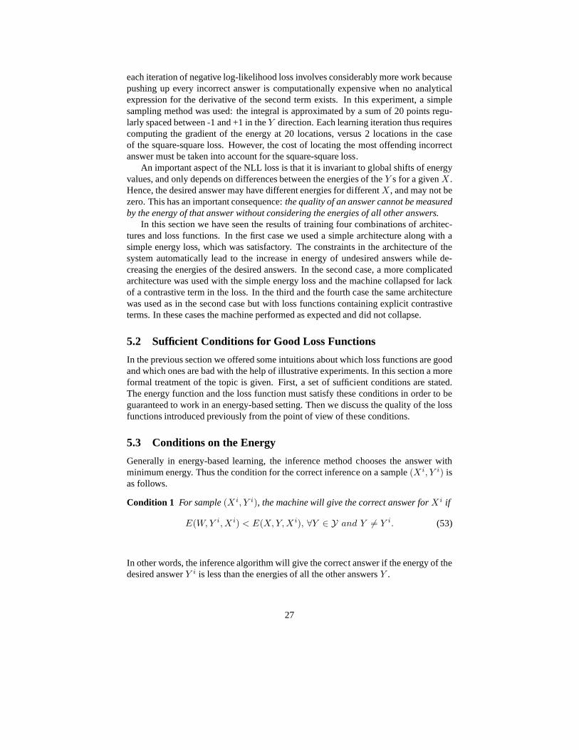
Generally in energy-based learning, the inference method chooses the answer withminimum energy. Thus the condition for the correct inference on a sample(X i, Y i) isas follows.

Condition 1 For sample(X i, Y i), the machine will give the correct answer forX i if

E(W, Y i, X i) < E(X, Y, X i), ∀Y ∈ Y and Y 6= Y i. (53)

In other words, the inference algorithm will give the correct answer if the energy of thedesired answerY i is less than the energies of all the other answersY .

27

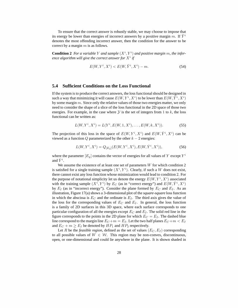
To ensure that the correct answer is robustly stable, we may choose to impose thatits energy be lower than energies of incorrect answers by a positive marginm. If Y i

denotes the most offending incorrect answer, then the condition for the answer to becorrect by a marginm is as follows.

Condition 2 For a variableY and sample(X i, Y i) and positive marginm, the infer-ence algorithm will give the correct answer forX i if

E(W, Y i, X i) < E(W, Y i, X i)−m. (54)

5.4 Sufficient Conditions on the Loss Functional

If the system is to produce the correct answers, the loss functional should be designed insuch a way that minimizing it will causeE(W, Y i, X i) to be lower thanE(W, Y i, X i)by some marginm. Since only the relative values of those two energies matter, we onlyneed to consider the shape of a slice of the loss functional inthe 2D space of those twoenergies. For example, in the case whereY is the set of integers from1 to k, the lossfunctional can be written as:

L(W, Y i, X i) = L(Y i, E(W, 1, X i), . . . , E(W, k, X i)). (55)

The projection of this loss in the space ofE(W, Y i, X i) andE(W, Y i, X i) can beviewed as a functionQ parameterized by the otherk − 2 energies:

L(W, Y i, X i) = Q[Ey](E(W, Y i, X i), E(W, Y i, X i)), (56)

where the parameter[Ey ] contains the vector of energies for all values ofY exceptY i

andY i.We assume the existence of at least one set of parametersW for which condition 2

is satisfied for a single training sample(X i, Y i). Clearly, if such aW does not exist,there cannot exist any loss function whose minimization would lead to condition 2. Forthe purpose of notational simplicity let us denote the energy E(W, Y i, X i) associatedwith the training sample(X i, Y i) by EC (as in “correct energy”) andE(W, Y i, X i)by EI (as in “incorrect energy”). Consider the plane formed byEC andEI . As anillustration, Figure 17(a) shows a 3-dimensional plot of thesquare-squareloss functionin which the abscissa isEC and the ordinate isEI . The third axis gives the value ofthe loss for the corresponding values ofEC and EI . In general, the loss functionis a family of 2D surfaces in this 3D space, where each surfacecorresponds to oneparticular configuration of all the energies exceptEC andEI . The solid red line in thefigure corresponds to the points in the 2D plane for whichEC = EI . The dashed blueline correspond to the margin lineEC+m = EI . Let the two half planesEC+m < EI

andEC + m ≥ EI be denoted byHP1 andHP2 respectively.Let R be thefeasible region, defined as the set of values(EC , EI) corresponding

to all possible values ofW ∈ W . This region may be non-convex, discontinuous,open, or one-dimensional and could lie anywhere in the plane. It is shown shaded in

28

0 0.1 0.2 0.3 0.4 0.5 0.6 0.7 0.8 0.9 10

0.1

0.2

0.3

0.4

0.5

0.6

0.7

0.8

0.9

1

Energy: EC

Ene

rgy:

EI

HP1

HP2

EC + m = E

I

EC = E

I

m

R

Figure 14:Figure showing the various regions in the plane of the two energiesEC andEI . EC

are the (correct answer) energies associated with(Xi, Y i), andEI are the (incorrect answer)energies associated with(Xi, Y i).

Figure 14. As a consequence of our assumption that a solutionexists which satisfiesconditions 2,R must intersect the half planeHP1.

Let two points(e1, e2) and (e′1, e′2) belong to the feasible regionR, such that

(e1, e2) ∈ HP1 (that is,e1 + m < e2) and(e′1, e′2) ∈ HP2 (that is,e′1 + m ≥ e′2). We

are now ready to present the sufficient conditions on the lossfunction.

Condition 3 Let (X i, Y i) be theith training example andm be a positive margin.Minimizing the loss functionL will satisfy conditions 1 or 2 if there exists at least onepoint(e1, e2) with e1 + m < e2 such that for all points(e′1, e

′2) with e′1 + m ≥ e′2, we

haveQ[Ey](e1, e2) < Q[Ey](e

′1, e

′2), (57)

whereQ[Ey] is given by

L(W, Y i, X i) = Q[Ey](E(W, Y i, X i), E(W, Y i, X i)). (58)

In other words, the surface of the loss function in the space of EC andEI should besuch that there exists at least one point in the part of the feasible regionR intersectingthe half planeHP1 such that the value of the loss function at this point is less than itsvalue at all other points in the part ofR intersecting the half planeHP2.

Note that this is only a sufficient condition and not a necessary condition. Theremay be loss functions that do not satisfy this condition but whose minimization stillsatisfies condition 2.

29

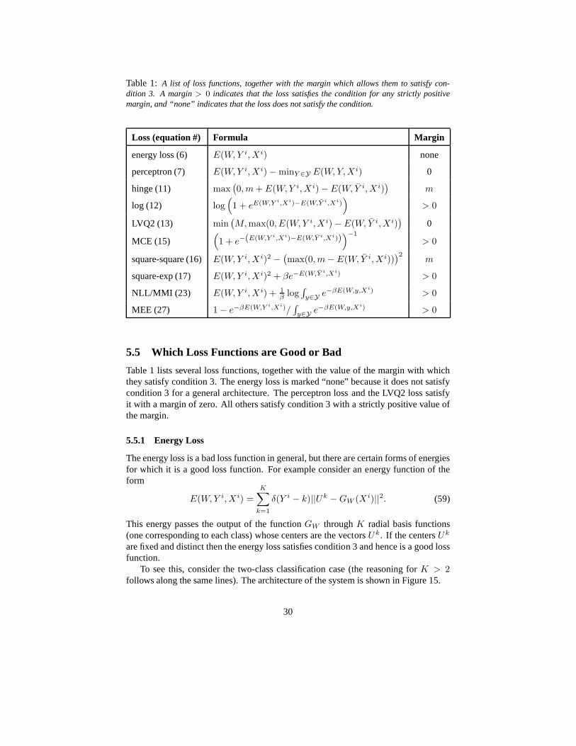
Table 1: A list of loss functions, together with the margin which allows them to satisfy con-dition 3. A margin> 0 indicates that the loss satisfies the condition for any strictly positivemargin, and “none” indicates that the loss does not satisfy the condition.

Loss (equation #) Formula Margin

energy loss (6) E(W, Y i, X i) none

perceptron (7) E(W, Y i, X i)−minY ∈Y E(W, Y, X i) 0

hinge (11) max(

0, m + E(W, Y i, X i)− E(W, Y i, X i))

m

log (12) log(

1 + eE(W,Y i,Xi)−E(W,Y i,Xi))

> 0

LVQ2 (13) min(

M, max(0, E(W, Y i, X i)− E(W, Y i, X i))

0

MCE (15)(

1 + e−(E(W,Y i,Xi)−E(W,Y i,Xi)))−1

> 0

square-square (16) E(W, Y i, X i)2 −(

max(0, m− E(W, Y i, X i)))2

m

square-exp (17) E(W, Y i, X i)2 + βe−E(W,Y i,Xi) > 0

NLL/MMI (23) E(W, Y i, X i) + 1β

log∫

y∈Y e−βE(W,y,Xi) > 0

MEE (27) 1− e−βE(W,Y i,Xi)/∫

y∈Y e−βE(W,y,Xi) > 0

5.5 Which Loss Functions are Good or Bad

Table 1 lists several loss functions, together with the value of the margin with whichthey satisfy condition 3. The energy loss is marked “none” because it does not satisfycondition 3 for a general architecture. The perceptron lossand the LVQ2 loss satisfyit with a margin of zero. All others satisfy condition 3 with astrictly positive value ofthe margin.

5.5.1 Energy Loss

The energy loss is a bad loss function in general, but there are certain forms of energiesfor which it is a good loss function. For example consider an energy function of theform

E(W, Y i, X i) =K∑

k=1

δ(Y i − k)||Uk −GW (X i)||2. (59)

This energy passes the output of the functionGW throughK radial basis functions(one corresponding to each class) whose centers are the vectorsUk. If the centersUk

are fixed and distinct then the energy loss satisfies condition 3 and hence is a good lossfunction.

To see this, consider the two-class classification case (thereasoning forK > 2follows along the same lines). The architecture of the system is shown in Figure 15.

30

X Y

GW (X)GW (X)

di = ||U i−GW (X)||2

d1 d2

GW

E(W,Y, X) =

2∑

k=1

δ(Y − k) · ||Uk−GW (X)||2

R B F U n i t s

Figure 15: The architecture of a system where two RBF units with centersU1 and U2 areplaced on top of the machineGW , to produce distancesd1 andd2.

(a) (b)

Figure 16:(a): When using the RBF architecture with fixed and distinct RBF centers, only theshaded region of the(EC , EI) plane is allowed. The non-shaded region is unattainable becausethe energies of the two outputs cannot be small at the same time. The minimum of the energyloss is at the intersection of the shaded region and verticalaxis. (b): The 3-dimensional plot ofthe energy loss when using the RBF architecture with fixed anddistinct centers. Lighter shadesindicate higher loss values and darker shades indicate lower values.

31

Letd = ||U1−U2||2, d1 = ||U1−GW (X i)||2, andd2 = ||U2−GW (X i)||2. SinceU1 andU2 are fixed and distinct, there is a strictly positive lower bound ond1 + d2

for all GW . Being only a two-class problem,EC andEI correspond directly to theenergies of the two classes. In the(EC , EI) plane no part of the loss function existsin whereEC + EI ≤ d. The region where the loss function is defined is shaded inFigure 16(a). The exact shape of the loss function is shown inFigure 16(b). One cansee from the figure that as long asd ≥ m, the loss function satisfies condition 3. Weconclude that this is a good loss function.

However, when the RBF centersU1 andU2 are not fixed and are allowed to belearned, then there is no guarantee thatd1 + d2 ≥ d. Then the RBF centers couldbecome equal and the energy could become zero for all inputs,resulting in a collapsedenergy surface. Such a situation can be avoided by having a contrastive term in the lossfunction.

5.5.2 Generalized Perceptron Loss

The generalized perceptron loss has a margin of zero. Therefore, it could lead to a col-lapsed energy surface and is not generally suitable for training energy-based models.However, the absence of a margin is not always fatal [LeCun etal., 1998a, Collins, 2002].First, the set of collapsed solutions is a small piece of the parameter space. Second,although nothing prevents the system from reaching the collapsed solutions, nothingdrives the system toward them either. Thus the probability of hitting a collapsed solu-tion is quite small.

5.5.3 Generalized Margin Loss

0

0.5

1

00.2

0.40.6

0.810

0.5

1

1.5

2

2.5

3

3.5

4

Energy: EC

Energy: EI

Loss

: L

HP2

EC = E

IEC + m = E

I

HP1 0

0.5

1

00.2

0.40.6

0.810

0.5

1

1.5

Energy: ECEnergy: E

I

Loss

: L

HP2

EC = E

IEC + m = E

I

HP1

(a) (b)

Figure 17: (a) The square-squareloss in the space of energiesEC and EI ). The value ofthe loss monotonically decreases as we move fromHP2 into HP1, indicating that it satisfiescondition 3. (b) Thesquare-exponentialloss in the space of energiesEC andEI ). The valueof the loss monotonically decreases as we move fromHP2 into HP1, indicating that it satisfiescondition 3.

32

We now consider thesquare-squareandsquare-exponentiallosses. For the two-class case, the shape of the surface of the losses in the spaceof EC andEI is shown inFigure 17. One can clearly see that there exists at least one point (e1, e2) in HP1 suchthat

Q[Ey](e1, e2) < Q[Ey](e′1, e

′2), (60)

for all points(e′1, e′2) in HP2. These loss functions satisfy condition 3.

5.5.4 Negative Log-Likelihood Loss

It is not obvious that the negative log-likelihood loss satisfies condition 3. The prooffollows.

0 0.1 0.2 0.3 0.4 0.5 0.6 0.7 0.8 0.9 10

0.1

0.2

0.3

0.4

0.5

0.6

0.7

0.8

0.9

1

Energy: EC

Ene

rgy:

EI

HP1

HP2

EC

+ m = EI

EC

= EI

m

R

gC

gI

g = gC

+ gI

−g

A = (E*C

, E*C

+ m)

B = (E*C

− ε, E*C

+ m + ε)

ε

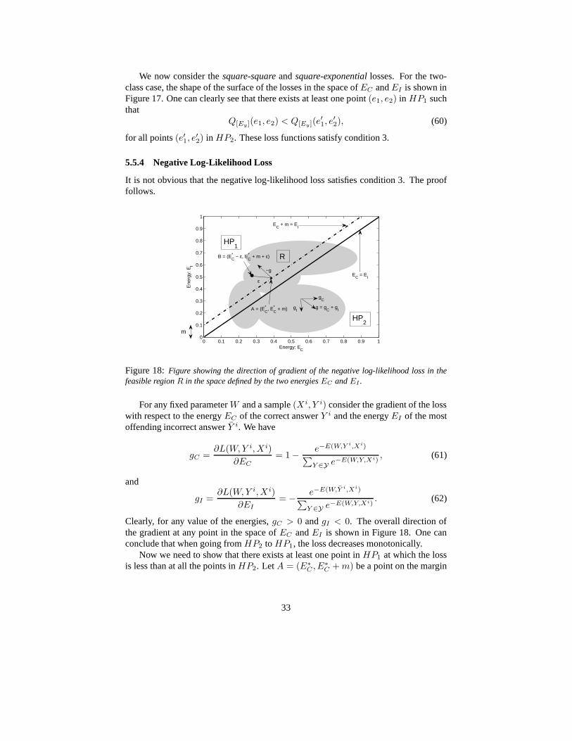
Figure 18:Figure showing the direction of gradient of the negative log-likelihood loss in thefeasible regionR in the space defined by the two energiesEC andEI .

For any fixed parameterW and a sample(X i, Y i) consider the gradient of the losswith respect to the energyEC of the correct answerY i and the energyEI of the mostoffending incorrect answerY i. We have

gC =∂L(W, Y i, X i)

∂EC

= 1−e−E(W,Y i,Xi)

∑

Y ∈Y e−E(W,Y,Xi), (61)

and

gI =∂L(W, Y i, X i)

∂EI

= −e−E(W,Y i,Xi)

∑

Y ∈Y e−E(W,Y,Xi). (62)

Clearly, for any value of the energies,gC > 0 andgI < 0. The overall direction ofthe gradient at any point in the space ofEC andEI is shown in Figure 18. One canconclude that when going fromHP2 to HP1, the loss decreases monotonically.

Now we need to show that there exists at least one point inHP1 at which the lossis less than at all the points inHP2. Let A = (E∗

C , E∗C + m) be a point on the margin

33

line for which the loss is minimum.E∗C is the value of the correct energy at this point.

That is,E∗

C = argmin{Q[Ey](EC , EC + m)}. (63)

Since from the above discussion, the negative of the gradient of the lossQ[Ey] at allpoints (and in particular on the margin line) is in the direction which is insideHP1, bymonotonicity of the loss we can conclude that

Q[Ey](E∗C , E∗

C + m) ≤ Q[Ey](EC , EI), (64)

whereEC + m > EI .Consider a pointB at a distanceǫ away from the point(E∗

C , E∗C + m), and inside

HP1 (see Figure 18). That is the point

(E∗C − ǫ, E∗

C + m + ǫ). (65)

Using the first order Taylor’s expansion on the value of the loss at this point, we get

Q[Ey](E∗C − ǫ, E∗

C + m + ǫ)

= Q[Ey](E∗C , E∗

C + m)− ǫ∂Q[Ey]

∂EC

+ ǫ∂Q[Ey]

∂EI

+ O(ǫ2)

= Q[Ey](E∗C , E∗

C + m) + ǫ

[

∂Q[Ey]

∂EC

+∂Q[Ey]

∂EI

]

−1

1

+ O(ǫ2). (66)

From the previous discussion the second term on the right hand side is negative. So forsufficiently smallǫ we have

Q[Ey](E∗C − ǫ, E∗

C + m + ǫ) < Q[Ey](E∗C , E∗

C + m). (67)

Thus we conclude that there exists at least one point inHP1 at which the loss is lessthan at all points inHP2.

Note that the energy of the most offending incorrect answerEI is bounded aboveby the value of the energy of the next most offending incorrect answer. Thus we onlyneed to consider a finite range ofEI ’s and the pointB cannot be at infinity.

6 Efficient Inference: Non-Probabilistic Factor Graphs

This section addresses the important issue of efficient energy-based inference. Se-quence labeling problems and other learning problem with structured outputs can oftenbe modeled using energy functions whose structure can be exploited for efficient infer-ence algorithms.

Learning and inference with EBMs involves a minimization ofthe energy over theset of answersY and latent variablesZ. When the cardinality ofY × Z is large, thisminimization can become intractable. One approach to the problem is to exploit thestructure of the energy function in order to perform the minimization efficiently. Onecase where the structure can be exploited occurs when the energy can be expressed as a

34

Y1 Y2

+

Z2Z1X

E(Y, Z, X)

Eb(X, Z1, Z2) Ec(Z2, Y1) Ed(Y1, Y2)Ea(X, Z1)

Y1 Y2Z2Z1

0 0 0

0

1 1 1 1

2

Ea (X

, 0)

Ea

(X, 1

)

Eb(X, 1, 1)

Eb (X

, 1, 0)

Eb(X, 0, 0)

E b(X

, 0, 1

)

0

0

0

Ec(1, 1)

Ec (1, 0)

E c(0

, 1)

Ec(0, 0) Ed(0, 0)

Ed(0

, 1)

Ed(1, 1)

Ed(1, 2

)

Ed (1, 0)

E d(0, 2

)

Figure 19:Top: A log domain factor graph. The energy is a sum of factors that take differ-ent subsets of variables as inputs. Bottom: Each possible configuration ofZ and Y can berepresented by a path in a trellis. HereZ1, Z2, andY1 are binary variables, whileY2 is ternary.

35

sum of individual functions (called factors) that each depend on different subsets of thevariables inY andZ. These dependencies are best expressed in the form of afactorgraph [Kschischang et al., 2001, MacKay, 2003]. Factor graphs area general form ofgraphical models, or belief networks.

Graphical models are normally used to represent probability distributions over vari-ables by directly encoding the dependency relationships between variables. At firstglance, it is difficult to dissociate graphical models from probabilistic modeling (wit-ness their original name: “Bayesian networks”). However, factor graphs can be studiedoutside the context of probabilistic modeling, and EBM learning applies to them.

A simple example of a factor graph is shown in Figure 19 (top).The energy func-tion is the sum of four factors:

E(Y, Z, X) = Ea(X, Z1) + Eb(X, Z1, Z2) + Ec(Z2, Y1) + Ed(Y1, Y2), (68)

whereY = [Y1, Y2] are the output variables andZ = [Z1, Z2] are the latent variables.Each factor can be seen as representing soft constraints between the values of its inputvariables. The inference problem consists in finding:

(Y , Z) = argminy∈Y, z∈Z (Ea(X, z1) + Eb(X, z1, z2) + Ec(z2, y1) + Ed(y1, y2)) .(69)

This factor graph represents astructured outputproblem, because the factorEd en-codes dependencies betweenY 1 andY 2 (perhaps by forbidding certain combinationsof values).

Let’s assume thatZ1, Z2, andY1 are discrete binary variables, andY2 is a ternaryvariable. The cardinality of the domain ofX is immaterial sinceX is always observed.The number of possible configurations ofZ andY givenX is 2 × 2 × 2 × 3 = 24.A naive minimization algorithm through exhaustive search would evaluate the entireenergy function 24 times (96 single factor evaluations). However, we notice that for agivenX , Ea only has two possible input configurations:Z1 = 0 andZ1 = 1. Sim-ilarly, Eb andEc only have 4 possible input configurations, andEd has 6. Hence,there is no need for more than2 + 4 + 4 + 6 = 16 single factor evaluations. The setof possible configurations can be represented by a graph (a trellis) as shown in Fig-ure 19 (bottom). The nodes in each column represent the possible values of a singlevariable. Each edge is weighted by the output energy of the factor for the correspond-ing values of its input variables. With this representation, a single path from the startnode to the end node represents one possible configuration ofall the variables. Thesum of the weights along a path is equal to the total energy forthe corresponding con-figuration. Hence, the inference problem can be reduced to searching for the shortestpath in this graph. This can be performed using a dynamic programming method suchas the Viterbi algorithm, or the A* algorithm. The cost is proportional to the numberof edges (16), which is exponentially smaller than the number of paths in general. TocomputeE(Y, X) = minz∈Z E(Y, z, X), we follow the same procedure, but we re-strict the graph to the subset of arcs that are compatible with the prescribed value ofY .

The above procedure is sometimes called themin-sum algorithm, and it is the logdomain version of the traditional max-product for graphical models. The procedure caneasily be generalized to factor graphs where the factors take more than two variables

36

as inputs, and to factor graphs that have a tree structure instead of a chain structure.However, it only applies to factor graphs that are bipartitetrees (with no loops). Whenloops are present in the graph, the min-sum algorithm may give an approximate solu-tion when iterated, or may not converge at all. In this case, adescent algorithm such assimulated annealing could be used.

As mentioned in Section 4, variables can be handled through minimization orthrough marginalization. The computation is identical to the one required for comput-ing the contrastive term of the negative log-likelihood loss (the log partition function),hence we will make no distinctions. The contrastive term in the negative log-likelihoodloss function is:

−1

βlog

∫

Y ∈Y, z∈Z

e−βE(Z,Y,X), (70)

or simply

−1

βlog

∫

Y ∈Y

e−βE(Y,X), (71)

when no latent variables are present.At first, this seems intractable, but the computation can be factorized just like with

the min-sum algorithm. The result is the so-calledforward algorithmin the log domain.Values are propagated forward, starting at the start node onthe left, and following thearrows in the trellis. Each nodek computes a quantityαk:

αk = −1

βlog∑

j

e−β(Ekj+αj), (72)

whereEjk is the energy attached to the edge linking nodej to nodek. The finalα atthe end node is the quantity in Eq. 70. The procedure reduces to the min-sum algorithmfor large values ofβ.

In a more complex factor graph with factors that take more than two variables as in-put, or that have a tree structure, this procedure generalizes to a non-probabilistic formof belief propagation in the log domain. For loopy graphs, the procedure can be iter-ated, and may lead to an approximate value for Eq. 70, if it converges at all [Yedidia et al., 2005].

The above procedures are an essential component for constructing models withstructures and/or sequential output.

6.1 EBMs versus Internally Normalized Models

It is important to note that at no point in the above discussion did we need to manip-ulate normalized probability distributions. The only quantities that are manipulatedare energies. This is in contrast with hidden Markov models and traditional Bayesiannets. In HMMs, the outgoing transition probabilities of a node must sum to 1, and theemission probabilities must be properly normalized. This ensures that the overall dis-tribution over sequences is normalized. Similarly, in directed Bayesian nets, the rowsof the conditional probability tables are normalized.

EBMs manipulate energies, so no normalization is necessary. When energies aretransformed into probabilities, the normalization overY occurs as the very last step

37

in the process. This idea oflate normalizationsolves several problems associatedwith the internal normalization of HMMs and Bayesian nets. The first problem is theso-calledlabel bias problem, first pointed out by Bottou [Bottou, 1991]: transitionsleaving a given state compete with each other, but not with other transitions in themodel. Hence, paths whose states have few outgoing transitions tend to have higherprobability than paths whose states have many outgoing transitions. This seems likean artificial constraint. To circumvent this problem, a latenormalization scheme wasfirst proposed by Denker and Burges in the context of handwriting and speech recogni-tion [Denker and Burges, 1995]. Another flavor of the label bias problem is themiss-ing probability mass problemdiscussed by LeCun et al. in [LeCun et al., 1998a]. Theyalso make use of a late normalization scheme to solve this problem. Normalized mod-els distribute the probability mass among all the answers that are explicitly modeled bythe system. To cope with “junk” or other unforeseen and un-modeled inputs, designersmust often add a so-calledbackground modelthat takes some probability mass awayfrom the set of explicitly-modeled answers. This could be construed as a thinly dis-guised way of removing the normalization constraint. To putit another way, sinceeveryexplicit normalization is another opportunity for mishandling unforeseen events, oneshould strive to minimize the number of explicit normalizations in a model. A recentdemonstration of successful handling of the label bias problem through normalizationremoval is the comparison between maximum entropy Markov models by McCallum,Freitag and Pereira [McCallum et al., 2000], and conditional random fields by Lafferty,McCallum and Pereira [Lafferty et al., 2001].

The second problem is controlling the relative importance of probability distribu-tions of different natures. In HMMs, emission probabilities are often Gaussian mix-tures in high dimensional spaces (typically 10 to 100), while transition probabilitiesare discrete probabilities over a few transitions. The dynamic range of the formeris considerably larger than that of the latter. Hence transition probabilities count foralmost nothing in the overall likelihood. Practitioners often raise the transition prob-abilities to some power in order to increase their influence.This trick is difficult tojustify in a probabilistic framework because it breaks the normalization. In the energy-based framework, there is no need to make excuses for breaking the rules. Arbitrarycoefficients can be applied to any subset of energies in the model. The normalizationcan always be performed at the end.

The third problem concerns discriminative learning. Discriminative training oftenuses iterative gradient-based methods to optimize the loss. It is often complicated, ex-pensive, and inefficient to perform a normalization step after each parameter update bythe gradient method. The EBM approach eliminates the problem [LeCun et al., 1998a].More importantly, the very reason for internally normalizing HMMs and Bayesian netsis somewhat contradictory with the idea of training them discriminatively. The normal-ization is only necessary for generative models.

38

7 EBMs for Sequence Labeling and Structured Out-puts

The problem of classifying or labeling sequences of symbolsor sequences of vec-tors has long been a topic of great interest in several technical communities. Theearliest and most notable example is speech recognition. Discriminative learningmethods were proposed to train HMM-based speech recognition systems in the late1980’s [Bahl et al., 1986, Ljolje et al., 1990]. These methods for HMMs brought abouta considerable improvement in the accuracy of speech recognition systems, and re-mains an active topic of research to this day.

With the appearance of multi-layer neural network trainingprocedures, severalgroups proposed combining neural networks and time alignment methods for speechrecognition. The time alignment was implemented either through elastic templatematching (Dynamic Time Warping) with a set of reference words, or using a hiddenMarkov model. One of the main challenges was to design an integrated trainingmethod for simultaneously training the neural network and the time alignment module.In the early 1990’s, several authors proposed such methods for combining neural netsand dynamic time warping [Driancourt et al., 1991a, Driancourt et al., 1991b,Driancourt and Gallinari, 1992b, Driancourt and Gallinari, 1992a,Driancourt, 1994], as well as for combining neural net and HMM[Bengio et al., 1990, Bourlard and Morgan, 1990, Bottou, 1991, Haffner et al., 1991,Haffner and Waibel, 1991, Bengio et al., 1992, Haffner and Waibel, 1992,Haffner, 1993, Driancourt, 1994, Morgan and Bourlard, 1995, Konig et al., 1996].Extensive lists of references on the topic are available in [McDermott, 1997,Bengio, 1996]. Most approaches used one dimensional convolutional net-works (time-delay neural networks) to build robustness to variations of pitch,voice timbre, and speed of speech. Earlier models combined discriminativeclassifiers with time alignment, but without integrated sequence-level train-ing [Sakoe et al., 1988, McDermott and Katagiri, 1992, Franzini et al., 1990].

Applying similar ideas to handwriting recognition proved more challenging, be-cause the 2D nature of the signal made the segmentation problem considerably morecomplicated. This task required the integration of image segmentation heuristics inorder to generate segmentation hypotheses. To classify thesegments with robust-ness to geometric distortions, 2D convolutional nets were used [Bengio et al., 1993,LeCun and Bengio, 1994, Bengio et al., 1995]. A general formulation of integratedlearning of segmentation and recognition with late normalization resulted in thegraphtransformer networkarchitecture [LeCun et al., 1997, LeCun et al., 1998a].

Detailed descriptions of several sequence labeling modelsin the framework ofenergy-based models are presented in the next three sections.

7.1 Linear Structured Models: CRF, SVMM, and MMMN

Outside of the discriminative training tradition in speechand handwriting recognition,graphical models have traditionally been seen as probabilistic generative models, andtrained as such. However, in recent years, a resurgence of interest for discriminative

39

E(W,Y, X)

f(X, Y1, Y2) f(X, Y2, Y3) f(X, Y3, Y4)

W1 W2 W3

Y1 Y2 Y3 Y4

X

+

Figure 20:A log domain factor graph for linear structured models, which include conditionalrandom fields, support vector Markov models, and maximum margin Markov networks.

training has emerged, largely motivated by sequence labeling problems in natural lan-guage processing, notably conditional random fields [Lafferty et al., 2001], perceptron-like models [Collins, 2002], support vector Markov models [Altun et al., 2003], andmaximum margin Markov networks [Taskar et al., 2003].

These models can be easily described in an EBM setting. The energy function inthese models is assumed to be a linear function of the parametersW :

E(W, Y, X) = WT F (X, Y ), (73)

whereF (X, Y ) is a vector of feature functions that depend onX andY . The answerY is a sequence ofl individual labels(Y1, . . . , Yl), often interpreted as a temporalsequence. The dependencies between individual labels in the sequence is captured by afactor graph, such as the one represented in Figure 20. Each factor is a linear functionof the trainable parameters. It depends on the inputX and on a pair of individual labels(Ym, Yn). In general, each factor could depend on more than two individual labels, butwe will limit the discussion to pairwise factors to simplifythe notation:

E(W, Y, X) =∑

(m,n)∈F

WTmnfmn(X, Ym, Yn). (74)

HereF denotes the set of factors (the set of pairs of individual labels that have a directinter-dependency),Wmn is the parameter vector for factor(m, n), andfmn(X, Ym, Yn)is a (fixed) feature vector. The global parameter vectorW is the concatenation of alltheWmn. It is sometimes assumed that all the factors encode the samekind of interac-tion between input and label pairs: the model is then called ahomogeneous field. The

40

factors share the same parameter vector and features, and the energy can be simplifiedas:

E(W, Y, X) =∑

(m,n)∈F

WT f(X, Ym, Yn). (75)

The linear parameterization of the energy ensures that the corresponding probabilitydistribution overW is in the exponential family:

P (W |Y, X) =e−W T F (X,Y )

∫

w′∈We−wT F (X,Y )

. (76)

This model is called thelinear structured model.We now describe various versions of linear structured models that use different loss

functions. Sections 7.2 and 7.3 will describe non-linear and hierarchical models.

7.1.1 Perceptron Loss

The simplest way to train the linear structured model is withthe perceptron loss. LeCunet al. [LeCun et al., 1998a] proposed its use for general, non-linear energy functionsin sequence labeling (particularly handwriting recognition), calling it discriminativeViterbi training. More recently, Collins [Collins, 2000, Collins, 2002] hasadvocatedits use for linear structured models in the context of NLP:

Lperceptron(W ) =1

P

P∑

i=1

E(W, Y i, X i)− E(W, Y ∗i, X i), (77)

whereY ∗i = argminy∈YE(W, y, X i) is the answer produced by the system. Thelinear property gives a particularly simple expression forthe loss:

Lperceptron(W ) =1

P

P∑

i=1

WT(

F (X i, Y i)− F (X i, Y ∗i))

. (78)

Optimizing this loss with stochastic gradient descent leads to a simple form of theperceptron learning rule:

W ←W − η(

F (X i, Y i)− F (X i, Y ∗i))

. (79)

As stated before, the main problem with the perceptron loss is the absence of margin,although this problem is not fatal when the energy is a linearfunction of the parameters,as in Collins’ model. The lack of a margin, which theoretically may lead to stabilityproblems, was overlooked in [LeCun et al., 1998a].

7.1.2 Margin Loss: Max-Margin Markov Networks

The main idea behind margin-based Markov networks [Altun etal., 2003,Altun and Hofmann, 2003, Taskar et al., 2003] is to use a margin loss to train

41

the linearly parameterized factor graph of Figure 20, with the energy function ofEquation 73. The loss function is the simple hinge loss with an L2 regularizer:

Lhinge(W ) =1

P

P∑

i=1

max(0, m + E(W, Y i, X i)− E(W, Y i, X i)) + γ||W ||2. (80)

Because the energy is linear inW , the loss becomes particularly simple:

Lhinge(W ) =1

P

P∑

i=1

max(

0, m + WT ∆F (X i, Y i))

+ γ||W ||2, (81)

where∆F (X i, Y i) = F (X i, Y i) − F (X i, Y i). This loss function can be optimizedwith a variety of techniques. The simplest method is stochastic gradient descent. How-ever, the hinge loss and linear parameterization allow for the use of a dual formulationas in the case of conventional support vector machines. The question of which op-timization method is most suitable is not settled. As with neural net training, it isnot clear whether second order methods bring a significant speed improvement overwell tuned stochastic gradient methods. To our knowledge, no systematic experimentalstudy of this issue has been published.

Altun, Johnson, and Hofman [Altun et al., 2003] have studiedseveral versions ofthis model that use other loss functions, such as the exponential margin loss proposedby Collins [Collins, 2000]:

Lhinge(W ) =1

P

P∑

i=1

exp(E(W, Y i, X i)− E(W, Y i, X i)) + γ||W ||2. (82)

This loss function tends to push the energiesE(W, Y i, X i) andE(W, Y i, X i) as farapart as possible, an effect which is moderated only by regularization.

7.1.3 Negative Log-Likelihood Loss: Conditional Random Fields

Conditional random fields(CRF) [Lafferty et al., 2001] use the negative log-likelihoodloss function to train a linear structured model:

Lnll(W ) =1

P

P∑

i=1

E(W, Y i, X i) +1

βlog∑

y∈Y

e−βE(W,y,Xi). (83)

The linear form of the energy (Eq. 75) gives the following expression:

Lnll(W ) =1

P

P∑

i=1

WT F (X i, Y i) +1

βlog∑

y∈Y

e−βW T F (Xi,y). (84)

Following Equation 24, the derivative of this loss with respect toW is:

∂Lnll(W )

∂W=

1

P

P∑

i=1

F (X i, Y i)−∑

y∈Y

F (X i, y)P (y|X i, W ), (85)

42

where

P (y|X i, W ) =e−βW T F (Xi,y)

∑

y′∈Y e−βW T F (Xi,y′). (86)

The problem with this loss function is the need to sum over allpossible label com-binations, as there are an exponentially large number of such combinations (2l for asequence ofl binary labels). However, one of the efficient inference algorithms men-tioned in Section 6 can be used.

One of the alleged advantages of CRFs is that the loss function is convex withrespect toW . However, the convexity of the loss function, while mathematically sat-isfying, does not seem to be a significant practical advantage. Although the originaloptimization algorithm for CRF was based on iterative scaling, recent work indicatesthat stochastic gradient methods may be more efficient [Vishwanathan et al., 2006].

7.2 Non-Linear Graph Based EBMs

The discriminative learning methods for graphical models developed in the speechand handwriting communities in the 90’s allowed for non-linear parameterizationsof the factors, mainly mixtures of Gaussians and multi-layer neural nets. Non-linearfactors allow the modeling of highly complex dependencies between inputs and labels(such as mapping the pixels of a handwritten word to the corresponding characterlabels). One particularly important aspect is the use of architectures that are invariant(or robust) to irrelevant transformations of the inputs, such as time dilation or pitchvariation in speech, and geometric variations in handwriting. This is best handled byhierarchical, multi-layer architectures that can learn low level features and higher levelrepresentations in an integrated fashion. Most authors have used one dimensionalconvolutional nets (time-delay neural networks) for speech and pen-based handwrit-ing [Bengio et al., 1990, Bottou, 1991, Haffner et al., 1991,Haffner and Waibel, 1991,Driancourt et al., 1991a, Driancourt et al., 1991b, Driancourt and Gallinari, 1992b,Driancourt and Gallinari, 1992a, Bengio et al., 1992, Haffner and Waibel, 1992,Haffner, 1993, Driancourt, 1994, Bengio, 1996], and 2D convolutional nets for image-based handwriting [Bengio et al., 1993, LeCun and Bengio, 1994, Bengio et al., 1995,LeCun et al., 1997, LeCun et al., 1998a].

To some observers, the recent interest in the linear structured model looks likesomewhat of a throw-back to the past, and a regression on the complexity scale. Oneapparent advantage of linearly parameterized energies is that they make the percep-tron loss, hinge loss, and NLL loss convex. It is often arguedthat convex loss func-tions are inherently better because they allow the use of efficient optimization algo-rithms with guaranteed convergence to the global minimum. However, several au-thors have recently argued that convex loss functions are noguarantee for good perfor-mance, and that non-convex losses may in fact be easier to optimize than convex onesin practice, even in the absence of theoretical guarantees [Huang and LeCun, 2006,Collobert et al., 2006].

Furthermore, it has been argued that convex loss functions can be effi-ciently optimized using sophisticated second-order optimization methods. How-ever, it is a well-known but often overlooked fact that a carefully tuned stochas-

43

tic gradient descent method is often considerably faster inpractice than eventhe most sophisticated second-order optimization methods(which appear bet-ter on paper). This is because stochastic gradients can takeadvantage ofthe redundancy between the samples by updating the parameters on the ba-sis of a single sample, whereas “batch” optimization methods waste consider-able resources to compute exact descent directions, often nullifying the theoreticalspeed advantage [Becker and LeCun, 1989, LeCun et al., 1998a, LeCun et al., 1998b,Bottou, 2004, Bottou and LeCun, 2004, Vishwanathan et al., 2006].

X Y

w o r d i nt h e l e x i c o nZ

E(W,Z, Y, X)

P a t h( a c o u s t i c v e c t o r s )w o r d t e m p l a t e s

f e a t u r e v e c t o r s

Figure 21:Figure showing the architecture of a speech recognition system using latent vari-ables. An acoustic signal is passed through a time-delay neural network (TDNN) to producea high level feature vector. The feature vector is then compared to the word templates. Dy-namic time warping (DTW) aligns the feature vector with the word templates so as to reduce thesensitivity of the matching to variations in pronunciation.

Figure 21 shows an example of speech recognition system thatintegrates a time-delay neural network (TDNN) and word matching using dynamictime warping (DTW).The raw speech signal is first transformed into a sequence of acoustic vectors (typically10 to 50 spectral or cepstral coefficients, every 10ms). The acoustic vector sequenceis fed to a TDNN that transforms it into a sequence of high level features. Temporalsubsampling in the TDNN can be used to reduce the temporal resolution of the fea-ture vectors [Bottou, 1991]. The sequence of feature vectors is then compared to wordtemplates. In order to reduce the sensitivity of the matching to variations in speed ofpronunciation, dynamic time warping aligns the feature sequence with the template se-quences. Intuitively, DTW consists in finding the best “elastic” warping that maps asequence of vectors (or symbols) to another. The solution can be found efficiently withdynamic programming (e.g. the Viterbi algorithm or the A* algorithm).

DTW can be reduced to a search for the shortest path in a directed acyclic graphin which the cost of each node is the mismatch between two items in the two in-

44

put sequences. Hence, the overall system can be seen as a latent variable EBM inwhich Y is the set of words in the lexicon, andZ represents the set of templatesfor each word, and the set of paths for each alignment graph. The earliest proposalfor integrated training of neural nets and time alignment isby Driancourt and Bot-tou [Driancourt et al., 1991a], who proposed using the LVQ2 loss (Eq. 13) to train thissystem. It is a simple matter to back-propagate gradients through the DTW moduleand further back-propagate gradients into the TDNN in orderto update the weights.Similarly, gradients can be back-propagated to the word templates in order to up-date them as well. Excellent results were obtained for isolated word recognition,despite the zero margin of the LVQ2 loss. A similar scheme waslater used by Mc-Dermott [McDermott, 1997].

A slightly more general method consists in combining neuralnetworks (e.g.TDNN) with hidden Markov models instead of DTW. Several authors proposedintegrated training procedures for such combinations during the 90’s. Thefirst proposals were by Bengio et al. [Bengio et al., 1991, Bengio et al., 1992,Bengio, 1996] who used the NLL/MMI loss optimized with stochastic gradient de-scent, and Bottou [Bottou, 1991] who proposed various loss functions. A simi-lar method was subsequently proposed by Haffner et al. in hismulti-state TDNNmodel [Haffner and Waibel, 1992, Haffner, 1993]. Similar training methods were de-vised for handwriting recognition. Bengio and LeCun described a neural net/HMMhybrid with global training using the NLL/MMI loss optimized with stochastic gradi-ent descent [Bengio et al., 1993, LeCun and Bengio, 1994]. Shortly thereafter, Koniget al. proposed the REMAP method, which applies the expectation maximization algo-rithm to the HMM in order to produce targets outputs for a neural net based acousticmodel [Konig et al., 1996].

The basic architecture of neural net/HMM hybrid systems is similar to the onein Figure 21, except that the word (or language) models are probabilistic finite-statemachines instead of sequences. The emission probabilitiesat each node are generallysimple Gaussians operating on the output vector sequences produced by the neural net.The only challenge is to compute the gradient of the loss withrespect to the neural netoutputs by backpropagating gradients through the HMM trellis. Since the procedure isvery similar to the one used in graph transformer networks, we refer to the next sectionfor a description.

It should be noted that many authors had previously proposedmethods that com-bined a separately trained discriminative classifier and analignment method for speechand handwriting, but they did not use integrated training methods.

7.3 Hierarchical Graph-Based EBMs: Graph Transformer Net-works

Sections 7.2 and 7.1 discussed models in which inference andlearning involved marginal-izing or minimizing over all configurations of variables of adynamic factor graph.These operations are performed efficiently by building a trellis in which each path cor-responds to a particular configuration of those variables. Section 7.2 concentrated onmodels where the factors are non-linear functions of the parameters, while Section 7.1

45

(a)

p a t hGW GW

P a t h S e l e c t o rV i t e r b iT r a n s f o r m e r

" 3 4 2 "R e c o g n i t i o nT r a n s f o r m e r

3 2 13 4 23 4

GW

X Y Z

E(W,Z, Y, X)

Grseg

Grint

Grsel

(b)

Figure 22:The architecture of agraph transformer networkfor handwritten word recognition.(a) The segmentation graphGrseg is generated from the input image, (b) the hierarchical multi-modular architecture takes a set of graphs and outputs another set of graphs.

focused on simpler models where the factors are linearly parameterized.The present section discusses a class of models calledgraph transformer networks

(GTN) [LeCun et al., 1998a]. GTNs are designed for situations where the sequentialstructure is so complicated that the corresponding dynamical factor graph cannot beexplicitly represented, but must be representedprocedurally. For example, the factor

46

graph that must be built on-the-fly in order to recognize an entire handwritten sen-tence in English is extremely large. The corresponding trellis contains a path for everygrammatically correct transcription of the sentence, for every possible segmentation ofthe sentence into characters. Generating this trellis (or its associated factor graph) inits entirety is impractical, hence the trellis must be represented procedurally. Insteadof representing the factor graph, the GTN approach views thetrellis as the main datastructure being manipulated by the machine. A GTN can be seenas a multilayer archi-tecture in which the states are trellises, just as a neural net is a multilayer architecture inwhich the states are fixed-size vectors. A GTN can be viewed asa network of modules,calledgraph transformers, that take one or more graphs as input and produces anothergraph as output. The operation of most modules can be expressed as the compositionof the input graph with another graph, called a transducer, associated with the mod-ule [Mohri, 1997]. The objects attached to the edges of the input graphs, which can benumbers, labels, images, sequences, or any other entity, are fed to trainable functionswhose outputs are attached to edge of the output graphs. The resulting architecturecan be seen as acompositional hierarchyin which low level features and parts arecombined into higher level objects through graph composition.

For speech recognition, acoustic vectors are assembled into phones, phones intotriphones, triphones into words, and words into sentences.Similarly in handwritingrecognition, ink segments are assembled into characters, characters into words, andwords into sentences.

Figure 22 shows an example of GTN architecture for simultaneously segmentingand recognizing handwritten words [LeCun et al., 1998a]. The first step involves over-segmenting the image and generating a segmentation graph out of it (see Figure 22(a)).The segmentation graphGrseg is a directed acyclic graph (DAG) in which each pathfrom the start node to the end node represents a particular way of segmenting the in-put image into character candidates. Each internal node is associated with a candidatecut produced by the segmentation. Every arc between a sourceand a destination nodeis associated with the part of the image that lies between thetwo cuts. Hence everypiece of ink appears once and only once along each path. The next stage passes thesegmentation graphGrseg through the recognition transformer which produces the in-terpretation graphGrint with the same number of nodes asGrseg . The recognitiontransformer contains as many identical copies of the discriminant functionsGW (X)as there are arcs in the interpretation graph (this number changes for every new in-put). Each copy ofGW takes the image associated with one arc in the segmentationgraph and produces several arcs between the corresponding nodes in the interpretationgraph. Each output arc is labeled by a character category, and weighted by the energyof assigning the image to that category. Hence, each path in the interpretation graphrepresents one possible interpretation of the input for onepossible segmentation, withthe sum of the weights along the path representing the combined energy of that inter-pretation. The interpretation graph is then passed througha path selector module thatselects only those paths from the interpretation graph thathave the same sequence oflabels as given byY (the answer). The output of this module is another graph calledGrsel. Finally a so-called Viterbi transformer selects a single path inGrsel indexed bythe latent variableZ. Each value ofZ corresponds to a different path inGrsel, and canbe interpreted as a particular segmentation of the input. The output energy is obtained

47

either by minimizing or by marginalizing overZ. Minimizing overZ is achieved byrunning a shortest path algorithm on theGrsel (e.g., the Viterbi algorithm, hence thename Viterbi transformer). The output energy is then the sumof the arc energies alongthe shortest path. Marginalizing overZ is achieved by running the forward algorithmon Grsel, as indicated in Section 6, equation 72. The path selector and Viterbi trans-former can be seen as particular types of “switch” modules that select paths in theirinput graph.

In the handwriting recognition systems described in [LeCunet al., 1998a], the dis-criminant functionGW (X) was a 2D convolutional network. This class of functionis designed to learn low level features and high level representations in an integratedmanner, and is therefore highly non-linear inW . Hence the loss function is not convexin W . The optimization method proposed is a refined version of stochastic gradientdescent.

In [LeCun et al., 1998a], two primary methods for training GTNs are proposed:discriminative Viterbi training, which is equivalent to using the generalized percep-tron loss (Eq. 7), anddiscriminative forward training, which is equivalent to using thenegative log-likelihood loss (Eq. 23). Any of the good losses in Table 1 could also beused.

Training by minimizing the perceptron loss with stochasticgradient descent is per-formed by applying the following update rule:

W ←W − η

(

∂E(W, Y i, X i)

∂W−

∂E(W, Y ∗i, X i)

∂W

)

. (87)

How can the gradients ofE(W, Y i, X i) andE(W, Y i, X i) be computed? The answeris simply to back-propagate gradients through the entire structure, all the way back tothe discriminant functionsGW (X). The overall energy can be written in the followingform:

E(W, Y, X) =∑

kl

δkl(Y )Gkl(W, X), (88)

where the sum runs over all arcs inGrint, Gkl(W, X) is the l-th component of thek copy of the discriminant function, andδkl(Y ) is a binary value equal to 1 if thearc containingGkl(W, X) is present in the final graph, and 0 otherwise. Hence, thegradient is simply:

∂E(W, Y, X)

∂W=∑

kl

δkl(Y )∂Gkl(W, X)

∂W. (89)

One must simply keep track of theδkl(Y ).In Section 5 we concluded that the generalized perceptron loss is not a good loss

function. While the zero margin may limit the robustness of the solution, the perceptronloss seems appropriate as a way to refine a system that was pre-trained on segmentedcharacters as suggested in [LeCun et al., 1998a]. Nevertheless, the GTN-based bankcheck reading system described in [LeCun et al., 1998a] thatwas deployed commer-cially was trained with the negative log-likelihood loss.

48

The second method for training GTNs uses the NLL loss function, with a marginal-ization overZ using the forward algorithm of Equation 72 overGrsel , instead of aminimization.

Training by minimizing the NLL loss with stochastic gradient descent is performedby applying the following update rule:

W ←W − η

(

∂FZ(W, Y i, X i)

∂W−

∂FY,Z(W, X i)

∂W

)

, (90)

where

FZ(W, Y i, X i) = −1

βlog∑

z∈Z

e−βE(W,Y i,z,Xi), (91)

is the free energy obtained by marginalizing overZ, keepingX i andY i fixed, and

FY,Z(W, X i) = −1

βlog

∑

y∈Y, z∈Z

e−βE(W,y,z,Xi), (92)

is the free energy obtained by marginalizing overY andZ, keepingX i fixed. Com-puting those gradients is slightly more complicated than inthe minimization case. Bychain rule the gradients can be expressed as:

∂FY,Z(W, X i)

∂W=∑

kl

∂FY,Z(W, X i)

∂Gkl

∂Gkl(W, X)

∂W, (93)

where the sum runs over all edges in the interpretation graph. The first factor is thederivative of the quantity obtained through the forward algorithm (Eq. 72) with respectto one particular edge in the interpretation graph. These quantities can be computed byback-propagating gradients through the trellis, viewed asa feed-forward network withnode functions given by Equation 72. We refer to [LeCun et al., 1998a] for details.

Contrary to the claim in [Lafferty et al., 2001], the GTN system trained with theNLL loss as described in [LeCun et al., 1998a] does assign a well-defined probabilitydistribution over possible label sequences. The probability of a particular interpretationis given by Equation 46:

P (Y |X) =

∫

z∈Ze−βE(Z,Y,X)

∫

y∈Y, z∈Z e−βE(y,z,X). (94)

It would seem natural to train GTNs with one of the generalized margin losses. Toour knowledge, this has never been done.

8 Discussion

There are still outstanding questions to be answered about energy-based and probabilis-tic models. This section offers a relatively philosophicaldiscussion of these questions,including an energy-based discussion of approximate methods for inference and learn-ing. Finally, a summary of the main ideas of this chapter is given.

49

8.1 EBMs and Probabilistic Models

In Section 1.3, the transformation of energies to probabilities through the Gibbs distri-bution was introduced:

P (Y |X, W ) =e−βE(W,Y,X)

∫

y∈Ye−βE(W,y,X)

. (95)

Any probability distribution overY can be approximated arbitrarily closely by a dis-tribution of that form. With finite energy values, distributions where the probabilityof someY is exactly zero can only be approximated. Estimating the parameters of aprobabilistic model can be performed in a number of different ways, including max-imum likelihood estimation with Bayes inversion, maximum conditional likelihoodestimation, and (when possible) Bayesian averaging (possibly with variational approx-imations). Maximizing the conditional likelihood of the training samples is equivalentto minimizing what we called the negative log-likelihood loss.

Hence, at a high level, discriminative probabilistic models can be seen as a specialcase of EBMs in which:

• The energy is such that the integral∫

y∈Y e−βE(W,y,X) (partition function) con-verges.

• The model is trained by minimizing the negative log-likelihood loss.

An important question concerns the relative advantages anddisadvantages of prob-abilistic models versus energy-based models. Probabilistic models have two majordisadvantages. First, the normalization requirement limits the choice of energy func-tions we can use. For example, there is no reason to believe that the model in Figure 7is normalizable overY . In fact, if the functionGW2

(Y ) is upper bounded, the integral∫ +∞

−∞e−βE(W,y,X)dy does not converge. A common fix is to include an additive term

Ry(Y ) to the energy, interpreted as a log prior onY , whose negative exponential isintegrable. Second, computing the contrastive term in the negative log-likelihood lossfunction (or its gradient with respect toW ) may be very complicated, expensive, oreven intractable. The various types of models can be dividedinto five rough categoriesof increasing complexity:

• Trivial : WhenY is discrete with a small cardinality, the partition function isa sum with a small number of terms that can be computed simply.Anothertrivial case is when the partition function does not depend on W , and hence canbe ignored for the purpose of learning. For example, this is the case when theenergy is a quadratic form inY with a fixed matrix. These are cases were theenergy loss can be used without fear of collapse.

• Analytical : When the partition function and its derivative can be computed an-alytically. For example, when the energy is a quadratic formin Y in which thematrix depends on trainable parameters, the partition function is a Gaussian in-tegral (with variable covariance matrix) and its derivative is an expectation undera Gaussian distribution, both of which have closed-form expressions.

50

• Computable: When the partition function is a sum over an exponential num-ber of terms, but the computation can be factorized in such a way as to make ittractable. The most notable case of this is when the partition function is a sumover configurations of output variables and latent variables of a tree-type graph-ical model. In this case, belief propagation can be used to compute the partitionfunction. When the graphical model is a simple chain graph (as in the case ofHMMs), the set of configurations can be represented by the paths of a weightedtrellis. Running the forward algorithm through this trellis yields the partitionfunction. A simple backpropagation-like procedure can be used to compute itsgradient (e.g., see [LeCun et al., 1998a] and reference therein).

• Approachable: When the partition function cannot be computed exactly, but canbe approximated reasonably well using various methods. Onenotable exampleis when the partition function is a sum over configurations ofa loopy graphi-cal model. The sum cannot be computed exactly, but loopy belief propagationor other variational methods may yield a suitable approximation. With those ap-proximations, the energies of the various answers will still be pulled up, althoughnot as systematically and with the same force as if using the full partition func-tion. In a sense, variational methods could be interpreted in the context of EBMas a way to choose a subset of energies to pull up.

• Intractable : When the partition function is truly intractable with no satisfactoryvariational approximation. In this case, one is reduced to usingsampling meth-ods. A sampling method is a policy for choosing suitable candidate answerswhose energy will be pulled up. The probabilistic approach to this is to sam-ple answers according to their probability under the model,and to pull up theirenergy. On average, each answer will be pulled up by the appropriate amountaccording to the partition function.

In this context, using an energy-based loss function other than the negative log-likelihoodcan be seen as a sampling method with a particular policy for picking the answerswhose energy will be pulled up. For example, the hinge loss systematically choosesthe most offending incorrect answer as the one whose energy should be pulled up. Inthe end, using such strategies will produce energy surfaceswith which differences ofenergies cannot be interpreted as likelihood ratios (the same is true with variationalmethods). We should emphasize again that this is inconsequential if the model is to beused for prediction, classification, or decision-making.

Variational approximation methods can be interpreted in the EBM framework asa particular choice of contrastive term for the loss function. A common approach isto view variational methods and energy-based loss functions as approximations to theprobabilistic method. What we propose here is to view the probabilistic approach asa special case of a much larger family of energy-based methods. Energy-based meth-ods are equally well justified as probabilistic methods. They are merely designed fortraining models to answer a different kind of question than probabilistic models.

An important open question is whether the variational methods that are commonlyused (e.g., mean field approximations with popular architectures) actually satisfy con-dition 3 (see Section 5.2).

51

8.2 Efficiency in Learning

The most important question that affects the efficiency of learning is: “How many en-ergies of incorrect answers must be explicitly pulled up before the energy surface takesthe right shape?”. Energy-based loss functions that pull upthe most offending incor-rect answer only pull up on a single energy at each learning iteration. By contrast, thenegative log-likelihood loss pulls up on all incorrect answers at each iteration, includ-ing those that are unlikely to produce a lower energy than thecorrect answer. Hence,unless the NLL computation can be done at very low cost (as in the case of “trivial”and “analytical” models), the energy-based approach is bound to be more efficient.

An important open question is whether alternative loss functions exist whose con-trastive term and its derivative are considerably simpler to compute than that of thenegative log-likelihood loss, while preserving the nice property that they pull up a largevolume of incorrect answers whose energies are “threateningly low”. Perhaps, a figureof merit for architectures and loss functions could be defined which would comparethe amount of computation required to evaluate the loss and its derivative relative tothe volume of incorrect answers whose energy is pulled up as aresult.

For models in the “intractable” category, each individual energy that needs to bepulled up or pushed down requires an evaluation of the energyand of its gradient(if a gradient-based optimization method is used). Hence, finding parameterizationsof the energy surface that will cause the energy surface to take the right shape withthe minimum amount of pushing of pulling is of crucial importance. IfY is high-dimensional, and the energy surface is infinitely malleable, then the energy surfacewill have to be pulled up in many places to make it take a suitable shape. Conversely,more “rigid” energy surfaces may take a suitable shape with less pulling, but are lesslikely to approach the correct shape. There seems to be a bias-variance dilemma similarto the one that influences the generalization performance.

8.3 Learning with Approximate Inference

Very often, the inference algorithm can only give us an approximate answer, or is notguaranteed to give us the global minimum of the energy. Can energy-based learningwork in this case? The theory for this does not yet exist, but afew intuitions may shedlight on the issue.

There may be certain answers inY that our inference algorithm never finds, per-haps because they reside in far-away regions of the space that the algorithm can neverreach. Our model may give low energy to wrong answers in theseregions, but since theinference algorithm cannot find them, they will never appearin the contrastive term,and their energies will never be pulled up. Fortunately, since those answers are notfound by the inference algorithm, we do not need to worry about their energies.

It is an interesting advantage of energy-based learning that only the incorrect an-swers whose energies are pulled up actually matter. This is in contrast with probabilis-tic loss functions (e.g. NLL) in which the contrastive term must pull up the energy ofevery single answer, including the ones that our inference algorithm will never find,which can be wasteful.

52

8.4 Approximate Contrastive Samples, Contrastive Divergence

Loss functions differ in how the contrastive sample is selected, and how hard its energyis pulled up. One interesting suggestion is to pull up on answers that are always near thecorrect answer, so as to make the correct answer a local minimum, but not necessarily aglobal one. This idea is the basis of thecontrastive divergence algorithmproposed byHinton [Hinton, 2002, Teh et al., 2003]. Contrastive divergence learning can be seenas an approximation of NLL learning with two shortcuts. First, the contrastive term inEquation 24 is approximated by drawing samples from the distribution P (Y |X i, W )using a Markov chain Monte Carlo method. Second, the samplesare picked by startingthe Markov chain at the desired answer, and by running only a few steps of the chain.This produces a sampleY i that is near the desired answer. Then, a simple gradientupdate of the parameters is performed:

W ←W − η

(

∂E(W, Y i, X i)

∂W−

∂E(W, Y i, X i)

∂W

)

. (96)

Since the contrastive sample is always near the desired answer, one can hope that thedesired answer will become a local minimum of the energy. Running MCMC for just afew steps limits computational expense. However, there is no guarantee that all incor-rect answers with low energy will be pulled up.

8.5 Conclusion

This tutorial was written to introduce and explicate the following major ideas:

• Many existing learning models can be be expressed simply in the framework ofenergy-based learning.

• Among the many loss functions proposed in the literature, some are good (witha non-zero margin), and some can be bad.

• Probabilistic learning is a special case of energy-based learning where the lossfunction is the negative log-likelihood, a.k.a. the maximum mutual informationcriterion.

• Optimizing the loss function with stochastic gradient methods is often more ef-ficient than black box convex optimization methods.

• Stochastic gradient methods can be applied to any loss function including non-convex ones. Local minima are rarely a problem in practice because of the highdimensionality of the space.

• Support vector Markov models, max-margin Markov networks,and conditionalrandom fields are all sequence modeling systems that use linearly parameterizedenergy factors. Sequence modeling systems with non-linearparameterization forspeech and handwriting recognition have been a very active research area sincethe early 1990’s. since the early 90’s.

53

• Graph transformer networks are hierarchical sequence modeling systems in whichthe objects that are manipulated are trellises containing all the alternative inter-pretations at a given level. Global training can be performed using stochasticgradient by using a form of back-propagation algorithm to compute the gradi-ents of the loss with respect to all the parameters in the system.

Acknowledgments

The authors wish to thank Geoffrey Hinton, Leon Bottou, Yoshua Bengio, SebastianSeung, and Brendan Frey for helpful discussions.

This work was supported in part by NSF ITR grant 0325463 “New directions inpredictive learning”.

References

[Altun and Hofmann, 2003] Altun, Y. and Hofmann, T. (2003). Large margin meth-ods for label sequence learning. InProc. of 8th European Conference on SpeechCommunication and Technology (EuroSpeech).

[Altun et al., 2003] Altun, Y., Johnson, M., and Hofmann, T. (2003). Loss functionsand optimization methods for discriminative learning of label sequences. InProc.EMNLP.

[Bahl et al., 1986] Bahl, L., Brown, P., de Souza, P., and Mercer, R. (1986). Maxi-mum mutual information estimation of hidden markov model parameters for speechrecognition. InProceedings of Acoustics, Speech, and Signal Processing Confer-ence, pages 49–52.

[Becker and LeCun, 1989] Becker, S. and LeCun, Y. (1989). Improving the conver-gence of back-propagation learning with second-order methods. In Touretzky, D.,Hinton, G., and Sejnowski, T., editors,Proc. of the 1988 Connectionist Models Sum-mer School, pages 29–37, San Mateo. Morgan Kaufman.

[Bengio, 1996] Bengio, Y. (1996).Neural Networks for Speech and Sequence Recog-nition. International Thompson Computer Press, London, UK.

[Bengio et al., 1990] Bengio, Y., Cardin, R., De Mori, R., andNormandin, Y. (1990).A hybrid coder for hidden markov models using a recurrent network. In Proceedingof ICASSP, pages 537–540.

[Bengio et al., 1992] Bengio, Y., De Mori, R., Flammia, G., and Kompe, R. (1992).Global optimization of a neural network-hidden Markov model hybrid. IEEE Trans-action on Neural Networks, 3(2):252–259.

[Bengio et al., 1991] Bengio, Y., DeMori, R., Flammia, G., and Kompe, R. (1991).Global optimization of a neural network - hidden markov model hybrid. In Pro-ceedings of EuroSpeech’91.

54

[Bengio et al., 2003] Bengio, Y., Ducharme, R., Vincent, P.,and Jauvin, C. (2003).A neural probabilistic language model.Journal of Machine Learning Research,3:1137–1155.

[Bengio and Frasconi, 1996] Bengio, Y. and Frasconi, P. (1996). An input/outputHMM architecture. In Tesauro, G., Touretzky, D., and Leen, T., editors,Advancesin Neural Information Processing Systems, volume 7, pages 427–434. MIT Press,Cambridge, MA.

[Bengio et al., 1993] Bengio, Y., LeCun, Y., and Henderson, D. (1993). Globallytrained handwritten word recognizer using spatial representation, space displace-ment neural networks and hidden markov models. In Cowan, J. and Tesauro, G.,editors,Advances in Neural Information Processing Systems, volume 6. MorganKaufmann.

[Bengio et al., 1995] Bengio, Y., LeCun, Y., Nohl, C., and Burges, C. (1995). Lerec:A nn/hmm hybrid for on-line handwriting recognition.Neural Computation,7(6):1289–1303.

[Bottou, 1991] Bottou, L. (1991).Une Approche theorique de l’Apprentissage Con-nexionniste: Applicationsa la Reconnaissance de la Parole. PhD thesis, Universitede Paris XI, 91405 Orsay cedex, France.

[Bottou, 2004] Bottou, L. (2004). Stochastic learning. In Bousquet, O. and vonLuxburg, U., editors,Advanced Lectures on Machine Learning, number LNAI 3176in Lecture Notes in Artificial Intelligence, pages 146–168.Springer Verlag, Berlin.

[Bottou and LeCun, 2004] Bottou, L. and LeCun, Y. (2004). Large-scale on-line learn-ing. In Advances in Neural Information Processing Systems 15. MIT Press.

[Bottou et al., 1997] Bottou, L., LeCun, Y., and Bengio, Y. (1997). Global trainingof document processing systems using graph transformer networks. In Proc. ofComputer Vision and Pattern Recognition, pages 490–494, Puerto-Rico. IEEE.

[Bourlard and Morgan, 1990] Bourlard, H. and Morgan, N. (1990). A continuousspeech recognition system embedding mlp into hmm. In Touretzky, D., editor,Ad-vances in Neural Information Processing Systems 2, pages 186–193. Morgan Kauf-mann.

[Bromley et al., 1993] Bromley, J., Guyon, I., LeCun, Y., Sackinger, E., and Shah, R.(1993). Signature verification using a siamese time delay neural network. In Cowan,J. and Tesauro, G., editors,Advances in Neural Information Processing Systems,volume 6. Morgan Kaufmann.

[Chopra et al., 2005] Chopra, S., Hadsell, R., and LeCun, Y. (2005). Learning a simi-larity metric discriminatively, with application to face verification. InProc. of Com-puter Vision and Pattern Recognition Conference. IEEE Press.

[Collins, 2000] Collins, M. (2000). Discriminative reranking for natural languageparsing. InProceedings of ICML 2000.

55

[Collins, 2002] Collins, M. (2002). Discriminative training methods for hiddenmarkov models: Theory and experiments with perceptron algorithms. In Proc.EMNLP.

[Collobert et al., 2006] Collobert, R., Weston, J., and Bottou, L. (2006). Trading con-vexity for scalability. InProceedings of the Twenty-third International Conferenceon Machine Learning (ICML 2006). IMLS/ICML. ACM Digital Library.

[Denker and Burges, 1995] Denker, J. S. and Burges, C. J. (1995). Image segmenta-tion and recognition. InThe Mathematics of Induction. Addison Wesley.

[Driancourt, 1994] Driancourt, X. (1994).Optimisation par descente de gradientstochastique de systemes modulaires combinant reseaux de neurones et programma-tion dynamique. Applicationa la reconnaissance de la parole. (optimization throughstochastic gradient of modular systems that combine neuralnetworks and dynamicprogramming, with applications to speech recognition). PhD thesis, Universite deParis XI, 91405 Orsay cedex, France.

[Driancourt et al., 1991a] Driancourt, X., Bottou, L., and Gallinari, P. (1991a). MLP,LVQ and DP: Comparison & cooperation. InProceedings of the International JointConference on Neural Networks, volume 2, pages 815–819, Seattle.

[Driancourt et al., 1991b] Driancourt, X., Bottou, L., and P., G. (1991b). Comparisonand cooperation of several classifiers. InProceedings of the International Confer-ence on Artificial Neural Networks (ICANN).

[Driancourt and Gallinari, 1992a] Driancourt, X. and Gallinari, P. (1992a). Empiricalrisk optimisation: neural networks and dynamic programming. In Proceedings ofNeural Networks for Signal Processing (NNSP).

[Driancourt and Gallinari, 1992b] Driancourt, X. and Gallinari, P. (1992b). A speechrecognizer optimaly combining learning vector quantization, dynamic programmingand multi-layer perceptron. InProceedings of ICASSP.

[Franzini et al., 1990] Franzini, M., Lee, K. F., and Waibel,A. (1990). Connection-nist viterbi training: A new hybrid method for continuous speech recognition. InProceedings of ICASSP, page 245.

[Hadsell et al., 2006] Hadsell, R., Chopra, S., and LeCun, Y.(2006). Dimensionalityreduction by learning an invariant mapping. InProc. Computer Vision and PatternRecognition Conference (CVPR’06). IEEE Press.

[Haffner, 1993] Haffner, P. (1993). Connectionist speech recognition with a globalMMI algorithm. In EUROSPEECH’93, 3rd European Conference on Speech Com-munication and Technology, Berlin.

[Haffner et al., 1991] Haffner, P., Franzini, M., and Waibel, A. H. (1991). Integrat-ing time-alignment and neural networks for high performance continuous speechrecognition. InProceeding of ICASSP, pages 105–108. IEEE.

56

[Haffner and Waibel, 1991] Haffner, P. and Waibel, A. H. (1991). Time-delayneural networks embedding time alignment: a performance analysis. In EU-ROSPEECH’91, 2nd European Conference on Speech Communication and Tech-nology, Genova, Italy.

[Haffner and Waibel, 1992] Haffner, P. and Waibel, A. H. (1992). Multi-state time-delay neural networks for continuous speech recognition. In Advances in NeuralInformation Processing Systems, volume 4, pages 579–588. Morgan Kaufmann, SanMateo.

[Hinton, 2002] Hinton, G. E. (2002). Training products of experts by minimizing con-trastive divergence.Neural Computation, 14:1771–1800.

[Huang and LeCun, 2006] Huang, F.-J. and LeCun, Y. (2006). Large-scale learningwith svm and convolutional nets for generic object categorization. InProc. Com-puter Vision and Pattern Recognition Conference (CVPR’06). IEEE Press.

[Juang et al., 1997] Juang, B.-H., Chou, W., and Lee, C.-H. (1997). Minimum clas-sification error rate methods for speech recognition.IEEE Transactions on Speechand Audio Processing, 5(3):257–265.

[Konig et al., 1996] Konig, Y., Bourlard, H., and Morgan, N. (1996). REMAP: Re-cursive estimation and maximization of A posteriori probabilities — applicationto transition-based connectionist speech recognition. InTouretzky, D. S., Mozer,M. C., and Hasselmo, M. E., editors,Advances in Neural Information ProcessingSystems, volume 8, pages 388–394. The MIT Press.

[Kschischang et al., 2001] Kschischang, F., Frey, B., and Loeliger, H.-A. (2001).Factor graphs and the sum-product algorithm.IEEE Trans. Information Theory,47(2):498–519.

[Kumar and Hebert, 2004] Kumar, S. and Hebert, M. (2004). Discriminative fieldsfor modeling spatial dependencies in natural images. In Thrun, S., Saul, L., andScholkopf, B., editors,Advances in Neural Information Processing Systems 16. MITPress, Cambridge, MA.

[Lafferty et al., 2001] Lafferty, J., McCallum, A., and Pereira, F. (2001). Conditionalrandom fields: Probabilistic models for segmenting and labeling sequence data. InProc. International Conference on Machine Learning (ICML).

[LeCun and Bengio, 1994] LeCun, Y. and Bengio, Y. (1994). word-level training ofa handwritten word recognizer based on convolutional neural networks. In IAPR,editor, Proc. of the International Conference on Pattern Recognition, volume II,pages 88–92, Jerusalem. IEEE.

[LeCun et al., 1997] LeCun, Y., Bottou, L., and Bengio, Y. (1997). Reading checkswith graph transformer networks. InInternational Conference on Acoustics, Speech,and Signal Processing, volume 1, pages 151–154, Munich. IEEE.

57

[LeCun et al., 1998a] LeCun, Y., Bottou, L., Bengio, Y., and Haffner, P. (1998a).Gradient-based learning applied to document recognition.Proceedings of the IEEE,86(11):2278–2324.

[LeCun et al., 1998b] LeCun, Y., Bottou, L., Orr, G., and Muller, K. (1998b). Efficientbackprop. In Orr, G. and K., M., editors,Neural Networks: Tricks of the trade.Springer.

[LeCun and Huang, 2005] LeCun, Y. and Huang, F. (2005). Loss functions for dis-criminative training of energy-based models. InProc. of the 10-th InternationalWorkshop on Artificial Intelligence and Statistics (AIStats’05).

[Ljolje et al., 1990] Ljolje, A., Ephraim, Y., and Rabiner, L. R. (1990). Estimation ofhidden markov model parameters by minimizing empirical error rate. InProc. ofInternational Conference on Acoustics, Speech, and SignalProcessing, pages 709–712.

[MacKay, 2003] MacKay, D. J. C. (2003). Information Theory, Inference,and Learning Algorithms. Cambridge University Press. Available fromhttp://www.inference.phy.cam.ac.uk/mackay/itila/.

[McCallum et al., 2000] McCallum, A., Freitag, D., and Pereira, F. (2000). Maximumentropy markov models for information extraction and segmetnation. InProc. In-ternational Conference on Machine Learning (ICML), pages 591–598.

[McDermott, 1997] McDermott, E. (1997). Discriminative Training for SpeechRecognition. PhD thesis, Waseda University.

[McDermott and Katagiri, 1992] McDermott, E. and Katagiri,S. (1992). Prototype-based discriminative training for various speech units. InProceedings of ICASSP-92, San Francisco, CA, USA, pages 417–420.

[Mohri, 1997] Mohri, M. (1997). Finite-state transducers in language and speech pro-cessing.Computational Linguistics, 23(2):269–311.

[Morgan and Bourlard, 1995] Morgan, N. and Bourlard, H. (1995). Continuousspeech recognition: An introduction to the hybrid hmm/connectionist approach.IEEE Signal Processing Magazine, 12(3):25–42.

[Ning et al., 2005] Ning, F., Delhomme, D., LeCun, Y., Piano,F., Bottou, L., and Bar-bano, P. (2005). Toward automatic phenotyping of developing embryos from videos.IEEE Transactions on Image Processing, 14(9):1360–1371. Special issue on Molec-ular and Cellular Bioimaging, to appear.

[Osadchy et al., 2005] Osadchy, R., Miller, M., and LeCun, Y.(2005). Synergisticface detection and pose estimation with energy-based model. In Advances in NeuralInformation Processing Systems (NIPS 2004). MIT Press.

[Sakoe et al., 1988] Sakoe, H., Isotani, R., Yoshida, K., Iso, K., and Watanabe, T.(1988). Speaker-independant word recognition using dynamic programming neu-ral networks. InProceedings of ICASSP-88, New York, pages 107–110.

58

[Solla et al., 1988] Solla, S., Levin, E., and Fleisher, M. (1988). Accelerated learningin layered neural networks.Complex Systems, 2(6):625–639.

[Taskar et al., 2003] Taskar, B., Guestrin, C., and Koller, D. (2003). Max-marginmarkov networks. InProc. NIPS.

[Teh et al., 2003] Teh, Y. W., Welling, M., Osindero, S., and E., H. G. (2003). Energy-based models for sparse overcomplete representations.Journal of Machine LearningResearch, 4:1235–1260.

[Vapnik, 1995] Vapnik, V. (1995).The Nature of Statistical Learning Theory. SpringerVerlag.

[Vishwanathan et al., 2006] Vishwanathan, S. V. N., Schraudolph, N. N., Schmidt,M. W., and Murphy, K. P. (2006). Accelerated training of conditional random fieldswith stochastic gradient methods. InProceedings of the Twenty-third InternationalConference on Machine Learning (ICML 2006). IMLS/ICML.

[Yedidia et al., 2005] Yedidia, J., Freeman, W., and Weiss, Y. (2005). Constructingfree-energy approximations and generalized belief propagation algorithms. IEEETransactions on Information Theory, 51(7):2282–2312.

59