a tutorial and case study in propensity score analysis: …hal.case.edu/~robrien/austin11a tutorial...

Multivariate Behavioral Research, 46:119–151, 2011

Copyright © Taylor & Francis Group, LLC

ISSN: 0027-3171 print/1532-7906 online

DOI: 10.1080/00273171.2011.540480

A Tutorial and Case Study in PropensityScore Analysis: An Application to

Estimating the Effect of In-HospitalSmoking Cessation Counseling

on Mortality

Peter C. Austin

Institute for Clinical Evaluative Sciences and University of Toronto

Propensity score methods allow investigators to estimate causal treatment effects

using observational or nonrandomized data. In this article we provide a practical

illustration of the appropriate steps in conducting propensity score analyses. For

illustrative purposes, we use a sample of current smokers who were discharged

alive after being hospitalized with a diagnosis of acute myocardial infarction. The

exposure of interest was receipt of smoking cessation counseling prior to hospital

discharge and the outcome was mortality with 3 years of hospital discharge. We

illustrate the following concepts: first, how to specify the propensity score model;

second, how to match treated and untreated participants on the propensity score;

third, how to compare the similarity of baseline characteristics between treated and

untreated participants after stratifying on the propensity score, in a sample matched

on the propensity score, or in a sample weighted by the inverse probability of

treatment; fourth, how to estimate the effect of treatment on outcomes when using

propensity score matching, stratification on the propensity score, inverse probability

of treatment weighting using the propensity score, or covariate adjustment using the

propensity score. Finally, we compare the results of the propensity score analyses

with those obtained using conventional regression adjustment.

Propensity score methods allow one to minimize the effects of observed con-

founding when estimating treatment effects using observational data. An article

Correspondence concerning this article should be addressed to Peter C. Austin, Institute for

Clinical Evaluative Sciences, G1 06, 2075 Bayview Avenue, Toronto, Ontario M4N 3M5 Canada.

E-mail: [email protected]

119

wiley-ds

Sticky Note

This is an open access article distributed under the Supplemental Terms and Conditions for iOpenAccess articles published in Taylor & Francis journals, which permits unrestricted use, distribution, and reproduction in any medium, provided the original work is properly cited.

120 AUSTIN

to appear in a special issue on propensity score analysis to be published in

Multivariate Behavioral Research describes a framework for using propensity

scores to estimate causal treatment effects using observational or nonrandomized

data (Austin, in press-a). In the review paper, the different methods of using

propensity scores to estimate treatment effects are highlighted along with a

description of the steps in conducting a propensity score analysis. The objective

of the current article is to illustrate the methods described in the overview article

using a single data source.

In this article, a propensity score analysis was conducted using four different

propensity score methods to estimate the effect of in-patient smoking cessation

counseling on mortality in patients hospitalized with a heart attack. The results

from the propensity score analyses are compared with those obtained using

conventional regression adjustment.

METHODS

Data Source

The data consisted of patients hospitalized with acute myocardial infarction

(AMI or heart attack) at 103 acute care hospitals in Ontario, Canada, between

April 1, 1999, and March 31, 2001. Data on patient history, cardiac risk factors,

comorbid conditions and vascular history, vital signs, and laboratory tests were

obtained by retrospective chart review by trained cardiovascular research nurses.

These data were collected as part of the Enhanced Feedback For Effective

Cardiac Treatment (EFFECT) study, an ongoing initiative intended to improve

the quality of care for patients with cardiovascular disease in Ontario (Tu et al.,

2004; Tu et al., 2009).

The sample was restricted to those patients who survived to hospital discharge

and who had documented evidence of being current smokers. For the purposes

of the current case study, the treatment or exposure of interest was whether

the patient received in-patient smoking cessation counseling. Smokers whose

counseling status could not be determined from the medical record were ex-

cluded from the current study. Patients with missing data on important baseline

clinical covariates were excluded from the sample. Patient records were linked

to the Registered Persons Database using encrypted health card numbers, which

allowed for determining the vital status of each patient at 3 years following

hospital discharge. For the current study, the outcome was survival to 3 years,

considered as both a dichotomous and a time-to-event outcome.

Baseline Comparisons of Treatment Groups

In the overall sample, continuous variables and categorical variables were com-

PROPENSITY SCORE METHODS 121

pared between treatment groups using the standard t test and chi-square test,

respectively. Standardized differences were also used to compare baseline char-

acteristics between the two groups (Austin, 2009a; Flury & Riedwyl, 1986).

Furthermore, basic baseline demographic characteristics and the probability of

death within 3 years of discharge were compared between participants with

complete data on baseline covariates and participants who were excluded from

the study sample due to missing data on baseline covariates.

Estimating the Propensity Score

An initial propensity score model was estimated using the 33 variables described

in Table 1. To estimate the propensity score, a logistic regression model was

used in which treatment status (receipt of smoking cessation counseling vs.

no smoking cessation counseling) was regressed on the baseline characteris-

tics listed in Table 1 (Rosenbaum & Rubin, 1984). The continuous baseline

variables were linearly related to the log-odds of receipt of treatment in the

initial specification of the propensity score model. Prior research on variable

selection for the propensity score suggests that it is preferable to either include

those variables that affect the outcome or include those variables that affect both

treatment selection and the outcome (Austin, Grootendorst, & Anderson, 2007).

The variables listed in Table 1 are plausible predictors of mortality in AMI

patients. Because we want to induce balance on variables that are prognostic of

mortality, we included these variables in our initial propensity score model.

Matching on the Propensity Score

Treated and untreated participants were matched on the propensity score. In the

data set, there were more treated participants (patients receiving smoking ces-

sation counseling) than there were untreated participants (patients not receiving

smoking cessation counseling). For technical reasons when matching, a pool

of controls that is at least as large as the number of treated participants was

required. Thus, in the context of propensity score matching, we attempted to

match a treated participant to each participant who did not receive smoking

cessation counseling. Thus, participants who received counseling were used as

a pool or reservoir from which to find appropriate participants to match to those

participants who did not receive counseling. Because propensity score matching

allows one to estimate the average treatment effect for the treated (ATT), this

implies that we are estimating the effect of smoking cessation counseling (or

the lack thereof) in those patients who ultimately did not receive such therapy

(Imbens, 2004).

For reasons described in the forthcoming review, participants were matched

on the logit of the propensity score (Rosenbaum & Rubin, 1985) using calipers

122 AUSTIN

TABLE 1

Baseline Characteristics of the Study Sample

Variable

No Smoking

Cessation

Counseling

(N D 754)

Smoking

Cessation

Counseling

(N D 1,588)

Overall

Sample

(N D 2,342)

Standardized

Difference of

the Mean p Value

Demographic Characteristics

Age 60.48 ˙ 13.26 56.24 ˙ 11.26 57.61 ˙ 12.10 0.35 < .001

Female 220 (29.2%) 397 (25.0%) 617 (26.3%) 0.09 .032

Presenting Signs and Symptoms

Acute pulmonary edema 34 (4.5%) 48 (3.0%) 82 (3.5%) 0.08 .067

Vital Signs on Admission

Systolic blood pressure 146.99 ˙ 31.82 146.93 ˙ 29.92 146.95 ˙ 30.53 0.00 .966

Diastolic blood pressure 84.81 ˙ 18.99 85.84 ˙ 18.51 85.50 ˙ 18.67 0.06 .213

Heart rate 83.28 ˙ 22.75 81.10 ˙ 22.54 81.80 ˙ 22.63 0.10 .029

Respiratory rate 21.18 ˙ 5.75 20.18 ˙ 4.64 20.50 ˙ 5.05 0.20 < .001

Classic Cardiac Risk Factors

Diabetes 179 (23.7%) 260 (16.4%) 439 (18.7%) 0.19 < .001

Hyperlipidemia 238 (31.6%) 539 (33.9%) 777 (33.2%) 0.05 .254

Hypertension 295 (39.1%) 541 (34.1%) 836 (35.7%) 0.11 .017

Family history of coronary artery disease 253 (33.6%) 754 (47.5%) 1,007 (43.0%) 0.28 < .001

Comorbid Conditions and Vascular History

Cerebrovascular accident/Transient

ischemic attack

62 (8.2%) 67 (4.2%) 129 (5.5%) 0.18 < .001

Angina 198 (26.3%) 412 (25.9%) 610 (26.0%) 0.01 .871

Cancer 22 (2.9%) 20 (1.3%) 42 (1.8%) 0.13 .005

Dementia 21 (2.8%) 6 (0.4%) 27 (1.2%) 0.23 < .001

Previous myocardial infarction 161 (21.4%) 241 (15.2%) 402 (17.2%) 0.16 < .001

Asthma 40 (5.3%) 98 (6.2%) 138 (5.9%) 0.04 .406

Depression 76 (10.1%) 131 (8.2%) 207 (8.8%) 0.06 .145

Peptic ulcer disease 39 (5.2%) 111 (7.0%) 150 (6.4%) 0.07 .093

Peripheral vascular disease 77 (10.2%) 90 (5.7%) 167 (7.1%) 0.18 < .001

Previous coronary revascularization 50 (6.6%) 92 (5.8%) 142 (6.1%) 0.04 .427

Chronic congestive heart failure 24 (3.2%) 24 (1.5%) 48 (2.0%) 0.12 .008

Laboratory Tests

Glucose 9.35 ˙ 5.63 8.57 ˙ 4.79 8.82 ˙ 5.09 0.15 < .001

White blood count 11.01 ˙ 4.49 10.77 ˙ 3.55 10.85 ˙ 3.88 0.06 .171

Hemoglobin 141.71 ˙ 19.33 145.83 ˙ 15.47 144.50 ˙ 16.92 0.24 < .001

Sodium 138.75 ˙ 4.54 139.40 ˙ 3.32 139.19 ˙ 3.77 0.17 < .001

Potassium 4.10 ˙ 0.58 4.01 ˙ 0.49 4.04 ˙ 0.52 0.16 < .001

Creatinine 99.59 ˙ 62.86 89.24 ˙ 30.24 92.57 ˙ 43.75 0.24 < .001

Prescriptions for Cardiovascular Medications at Hospital Discharge

Statin 193 (25.6%) 637 (40.1%) 830 (35.4%) 0.31 < .001

Beta-blocker 460 (61.0%) 1,192 (75.1%) 1,652 (70.5%) 0.31 < .001

Angiotensin Converting Enzyme (ACE)

inhibitor/Angiotensin receptor blockers

344 (45.6%) 850 (53.5%) 1,194 (51.0%) 0.16 < .001

Plavix 29 (3.8%) 74 (4.7%) 103 (4.4%) 0.04 .37

Acetylsalicyclic Acid (ASA) 544 (72.1%) 1,341 (84.4%) 1,885 (80.5%) 0.31 < .001

Note. Continuous variables are presented as means ˙ standard deviation; dichotomous variables are presented as N (%).


of width equal to 0.2 of the standard deviation of the logit of the estimated

propensity score. This caliper width has been found to result in optimal estima-

tion of risk differences in a variety of settings (Austin, 2010a).

In those participants who did not receive smoking cessation counseling,

differences in baseline covariates between matched and unmatched participants

were examined using statistical significance testing and standardized differences.

Inverse Probability of Treatment Weighting

We weighted the entire study sample by inverse probability of treatment weights

derived from the propensity score. Let Z denote treatment status (Z D 1 denotes

treated; Z D 0 denotes untreated) and let e denote the estimated propensity

score. Then the inverse probability of treatment weights are defined by Ze

C 1�Z1�e

.

Stratification on the Propensity Score

Using the entire study sample, we computed the quintiles of the estimated

propensity score. Participants in the overall study sample were stratified into five

approximately equal-size groups using the quintiles of the estimated propensity

score.

Balance Diagnostics

As discussed in the forthcoming review article, the true propensity score is a

balancing score: conditional on the true propensity score, treated and untreated

participants will have the same distribution of measured baseline covariates.

However, the true propensity score model is not known in observational studies

(unlike randomized experiments in which the true propensity score is often

defined by the study design). Thus, balance diagnostics allow one to assess

whether the propensity score model has been adequately specified. Appropriate

balance diagnostics are highlighted in our forthcoming review and are described

in greater detail elsewhere (Austin, 2009b).

Propensity score matched sample. We compared the means and preva-

lences of continuous and dichotomous baseline covariates between treatment

groups in the matched sample. The standardized difference was used to quantify

differences in means or prevalences between treatment groups. Furthermore,

we compared balance between treatment groups in all pairwise interactions of

continuous covariates. The variance of continuous variables was compared be-

tween treatment groups in the matched sample. Finally, cumulative density plots

and quantile-quantile plots were used to compare the distribution of continuous

baseline covariates between treatment groups.

124 AUSTIN

The reader should note that statistical significance testing was not used to

compare the baseline characteristics of treated and untreated participants in

the propensity score matched sample. Such practices have been criticized by

different authors. Readers are referred elsewhere for a greater discussion of this

practice (Austin, 2007a, 2008a, 2008b; Ho, Imai, King, & Stuart, 2007; Imai,

King, & Stuart, 2008).

Diagnostics based on comparing the distribution of the propensity score

between treated and untreated participants were not used. Recent research has

shown that, in the context of propensity score matching, comparing the distribu-

tion of the estimated propensity score between treated and untreated participants

does not provide any information as to whether the propensity score model has

been adequately specified (Austin, 2009b). For similar reasons, the c statistic

(equivalent to the area under the receiver operating characteristic [ROC] curve)

of the propensity score model was not reported. The c statistic does not provide

information as to whether the propensity score model has been adequately

specified (Austin, 2009b; Weitzen, Lapane, Toledano, Hume, & Mor, 2005).

Stratification on the propensity score. Within each stratum of the propen-

sity score, standardized differences were used to compare the means and preva-

lences of measured baseline covariates between treatment groups. Within-quintile

standardized differences were computed for each of the 55 pairwise interactions

between continuous variables.

Inverse probability of treatment weighting. In the sample weighted by the

inverse probability of treatment, we computed standardized differences to com-

pare the balance of baseline covariates between treatment groups. We also used

standardized differences to compare balance on pairwise interactions between

continuous baseline covariates. Empirical cumulative distribution functions and

quantile-quantile plots were also used to compare the distribution of continuous

baseline covariates between treatment groups in the weighted sample.

Covariate adjustment using the propensity score. Austin (2008c) de-

scribed the weighted conditional absolute standardized difference for comparing

balance in baseline covariates after adjusting for the propensity score. Briefly,

a given baseline covariate is regressed on the following three variables: the

propensity score, an indicator variable denoting treatment assignment, and the in-

teraction between the first two variables. Linear regression is used for continuous

covariates, whereas logistic regression is used for dichotomous covariates. From

the fitted regression model, for a given value of the propensity score, the mean

response is determined assuming a participant was treated and then assuming

the participant was untreated. The absolute standardized difference between the

mean response for treated participants and the mean response for untreated


participants is then determined. For continuous outcomes, this calculation will

also use the estimate of the variance of the error term that was obtained from the

linear model. This conditional (on the propensity score) absolute standardized

difference is then integrated over the distribution of the propensity score in the

study sample.

A second balance diagnostic involves the use of quantile regression (Austin,

Tu, Daly, & Alter, 2005). For a given continuous baseline covariate, quantile

regression was used to regress the given baseline covariate on the estimated

propensity score in treated and untreated participants separately. The use of the

5th, 25th, 50th, 75th, and 95th percentiles has been previously suggested (Austin,

2008c). The model-based estimates of these quantiles in treated and untreated

participants can then be displayed graphically.

Estimating Treatment Effects

As noted earlier, we considered two different outcomes: survival to 3 years post-

discharge (a dichotomous outcome) and time to death (a time-to-event outcome)

with participants censored at 3 years following hospital discharge.

Propensity score matching. The difference in the probability of 3-year

mortality between treatment groups was estimated by directly estimating the dif-

ference in proportions between treated and untreated participants in the propen-

sity score matched sample. When estimating the statistical significance of treat-

ment effects, the use of methods that account for the matched nature of the

sample is recommended (Austin, 2009d, in press-b). Accordingly, McNemar’s

test was used to assess the statistical significance of the risk difference. Confi-

dence intervals were constructed using a method proposed by Agresti and Min

(2004) that accounts for the matched nature of the sample. The number needed

to treat (NNT) is the reciprocal of the absolute risk reduction. The relative

risk was estimated as the ratio of the probability of 3-year mortality in treated

participants compared with that of untreated participants in the matched sample.

Methods described by Agresti and Min were used to estimate 95% confidence

intervals.

We then estimated the effect of provision of smoking cessation counseling on

the time to death. Kaplan-Meier survival curves were estimated separately for

treated and untreated participants in the propensity score matched sample. The

log-rank test is not appropriate for comparing the Kaplan-Meier survival curves

between treatment groups because the test assumes two independent samples

(Harrington, 2005; Klein & Moeschberger, 1997). However, the stratified log-

rank test is appropriate for matched pairs data (Klein & Moeschberger, 1997).

Finally, we used a Cox proportional hazards model to regress survival time

on an indicator variable denoting treatment status (smoking cessation counseling

126 AUSTIN

vs. no counseling). As the propensity score matched sample does not consist

of independent observations, we used a marginal survival model with robust

standard errors (Lin & Wei, 1989). An alternative to the use of a marginal model

with robust variance estimation would be to fit a Cox proportional hazards model

that stratified on the matched pairs (Cummings, McKnight, & Greenland, 2003).

This approach accounts for the within-pair homogeneity by allowing the baseline

hazard function to vary across matched sets.

Stratification on the propensity score. We estimated the probability of

3-year mortality for participants in each treatment group in each propensity

score strata. The absolute reduction in the probability of 3-year mortality was

then determined in each propensity score strata by the difference between the

observed probability for treated participants and the observed participants for

untreated participants within that stratum. The overall estimated treatment effect

was the mean of the stratum-specific risk differences. The standard error of

each stratum-specific risk difference can be estimated using standard methods

for differences in two binomial proportions. The stratum-specific standard errors

can then be pooled to obtain the standard error of the overall risk difference. We

also obtained the Mantel-Haenszel estimate of the pooled relative risk across

the propensity score strata (Breslow & Day, 1987).

To estimate the effect of counseling on survival, we used a Cox proportional

hazards model to regress survival time on treatment status. The model stratified

on the propensity score strata, allowing the baseline hazard to vary across the

strata.

As a sensitivity analysis, we also stratified the entire study sample into 10

approximately equal-size groups using the deciles of the estimated propensity

score.

Propensity score weighting. We estimated the absolute reduction in the

probability of mortality within 3 years of hospital discharge due to receipt of

in-patient smoking cessation counseling using a method described by Lunceford

and Davidian (2004). As mentioned earlier, let Zi be an indicator variable

denoting whether or not the i th participant was treated; furthermore, let ei

denote the propensity score for the i th participant. The weights are defined

as wi D Zi

eiC

.1�Zi /

1�ei. Assume that Yi denotes the outcome variable measured

on the i th participant. The first estimate of the average treatment effect (ATE) is1n

PniD1

Zi Yi

ei� 1

n

PniD1

.1�Zi /Yi

1�ei, where n denotes the number of participants in

the full sample. Lunceford and Davidian also provide estimates of the standard

error of the estimated treatment effect.

We used a second weighted estimator, also described by Lunceford and

Davidian (2004), from the family of doubly robust estimators. This estimator

requires specifying the propensity score model and regression models relating


the expected outcome to baseline covariates in treated and untreated subjects

separately. Let mz.X; ’z/ D E.Y jZ D z; X/. Then

O�DR D1

N

NX

iD1

Zi Yi � .Zi � Oei /m1.Xi ; O’/

Oei

�1

N

NX

iD1

.1 � Zi /Yi � .Zi � Oei/m0.Xi ; O’/

1 � Oei

:

O�DR has a “double-robustness” property in that the estimator remains consistent

if either the propensity score model is correctly specified or if both the outcomes

regression models are correctly specified (Lunceford & Davidian, 2004). For the

outcomes-regression models, we used logistic regression models in which the

dichotomous outcome was regressed on the 33 baseline covariates described in

Table 1.

We then used an approach similar to the aforementioned to estimate the

relative reduction in the probability of mortality within 3 years. Each of the es-

timators described by Lunceford and Davidian (2004) were modified to estimate

the relative risk rather than the difference in risks. Confidence intervals were

estimated using nonparametric bootstrap methods with 1,000 bootstrap samples.

We then used logistic regression to regress survival to 3 years (a dichotomous

outcome) on an indicator variable denoting receipt of in-patient smoking ces-

sation counseling in the weighted sample. Standard errors were obtained using

a robust variance estimate (Joffe, Ten Have, Feldman, & Kimmel, 2004). The

logistic regression model was then modified by adjusting for the 33 variables in

Table 1.

Our second outcome was time to death with participants censored at 3 years

after hospital discharge. We used two different methods to estimate the effect

of smoking cessation counseling on time to death in the weighted sample. First,

we fit a Cox proportional hazards model with counseling as the only predictor

variable. We used the inverse probability of treatment weights. Furthermore, we

used a robust sandwich variance estimator to account for the weighted nature

of the sample. Our second approach was based on the method of Xie and

Liu (2005) to estimate adjusted Kaplan-Meier estimates of survival curves in a

sample weighted by the inverse probability of treatment. Xie and Liu proposed

a weighted version of the log-rank test to test the null hypothesis that the two

survival curves are equal to one another.

Covariate adjustment using the propensity score. We considered two

different approaches to using covariate adjustment using the propensity score.

The first approach is based on regressing the outcome on two independent

128 AUSTIN

variables: an indicator variable denoting treatment assignment and the estimated

propensity score. For the binary outcome (survival to 3 years postdischarge) a

logistic regression model was used, whereas for the time-to-event outcome, a

Cox proportional hazards regression model was used.

The aforementioned two approaches, although common in the medical lit-

erature, have been shown to result in biased estimates of conditional odds

ratios and hazards ratios (Austin, Grootendorst, Normand, & Anderson, 2007).

Furthermore, the aforementioned approach for binary outcomes has also been

shown to result in biased estimation of marginal odds ratios (Austin, 2007b).

Thus, we implemented an approach based on one described by Imbens (2004).

This approach is similar to one described by Austin (2010b) for estimating

marginal treatment effects using logistic regression models. The aforementioned

logistic regression model was fit to the sample. Then for each participant, two

predicted probabilities were obtained: the probability of the outcome if the

participant had been treated and the probability of the outcome if the participant

had been untreated. The average probability of the outcome if untreated can then

be determined over all participants in the full study sample. Similarly, the average

probability of the outcome if treated can then be determined over all participants

in the sample. The difference between these two probabilities is the average

treatment effect (Imbens, 2004). Confidence intervals were obtained using non-

parametric bootstrap techniques (Efron & Tibshirani, 1993). A similar approach

can be used to estimate the relative reduction in death due to smoking cessation

counseling. The aforementioned approach can be replicated for the time-to-event

outcome (Austin, 2010c). Using this approach, one can determine the absolute

reduction in the probability of an event occurring within a specified duration of

follow-up.

Regression Adjustment

For comparative purposes, we used regression adjustment to estimate the effect

of smoking cessation counseling on mortality. First, logistic regression was used

to regress an indicator variable denoting survival to 3 years postdischarge on

an indicator variable denoting receipt of smoking cessation counseling and the

33 baseline covariates listed in Table 1. The logistic regression model was then

modified by using restricted cubic smoothing splines to model the relationship

between continuous baseline covariates and the log-odds of mortality.

We then used a Cox proportional hazards model to regress survival time on

treatment status and the 33 baseline covariates listed in Table 1. We then modified

the Cox proportional hazards model by using restricted cubic smoothing splines

to model the relationship between continuous baseline covariates and the log-

hazard of mortality.


RESULTS

Sample Description

The study sample for this case study consisted of 2,342 participants, of whom

1,588 received in-patient smoking cessation counseling and 754 did not. The

baseline characteristics of exposed and unexposed participants are described in

Table 1. Patients receiving smoking cessation counseling tended to be younger

.p < :001/, were less likely to be female .p D :032/, tended to have a lower

burden of comorbid conditions, and were more likely to receive prescriptions

for cardiac medications at hospital discharge compared with patients who did

not receive in-patient smoking cessation counseling. There were statistically

significant differences in 22 of the 33 baseline characteristics between exposed

and unexposed participants in the study sample. Twenty of the variables had

standardized differences that exceeded 0.10. Thus, as is typical in observational

studies, there were systematic differences in baseline characteristics between

treated and untreated patients.

There were no statistically significant differences in basic demographic char-

acteristics (age and sex) and in the probability of death within 3 years of

discharge between participants with complete data on baseline covariates and

participants who were excluded due to missing data on baseline covariates.

Matching on the Propensity Score

The standard deviation of the logit of the propensity score was equal to 0.7013542.

Thus, 0.2 of the standard deviation of the logit of the propensity score was

equal to 0.14027084. Therefore, matched treated and untreated participants

were required to have logits of the propensity score that differed by at most

0.14027084.

When participants who received in-patient smoking cessation counseling were

matched with participants who did not receive smoking cessation counseling on

the logit of the initially specified propensity score model, 682 matched pairs

were formed. Thus, 90% of patients who did not receive in-patient smoking

cessation counseling were successfully matched to a patient who did receive

in-patient smoking cessation counseling.

Balance Diagnostics

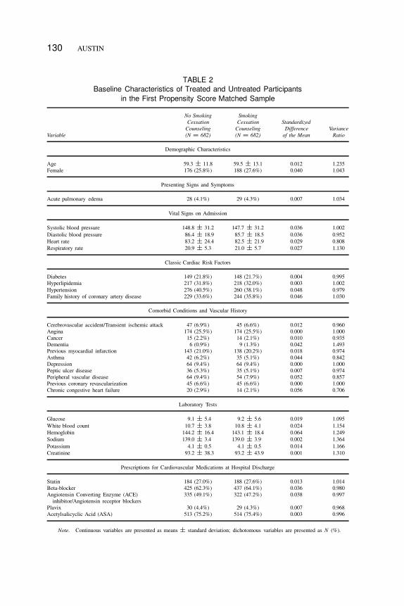
Propensity score matching. The baseline characteristics of patients re-

ceiving in-patient smoking cessation counseling and those not receiving coun-

seling in the initial propensity score matched sample are described in Table 2.

Across the 33 baseline covariates, the absolute standardized differences ranged

130 AUSTIN

TABLE 2

Baseline Characteristics of Treated and Untreated Participants

in the First Propensity Score Matched Sample

Variable

No Smoking

Cessation

Counseling

(N D 682)

Smoking

Cessation

Counseling

(N D 682)

Standardized

Difference

of the Mean

Variance

Ratio


Age 59.3 ˙ 11.8 59.5 ˙ 13.1 0.012 1.235

Female 176 (25.8%) 188 (27.6%) 0.040 1.043


Acute pulmonary edema 28 (4.1%) 29 (4.3%) 0.007 1.034


Systolic blood pressure 148.8 ˙ 31.2 147.7 ˙ 31.2 0.036 1.002

Diastolic blood pressure 86.4 ˙ 18.9 85.7 ˙ 18.5 0.036 0.952

Heart rate 83.2 ˙ 24.4 82.5 ˙ 21.9 0.029 0.808

Respiratory rate 20.9 ˙ 5.3 21.0 ˙ 5.7 0.027 1.130


Diabetes 149 (21.8%) 148 (21.7%) 0.004 0.995

Hyperlipidemia 217 (31.8%) 218 (32.0%) 0.003 1.002

Hypertension 276 (40.5%) 260 (38.1%) 0.048 0.979

Family history of coronary artery disease 229 (33.6%) 244 (35.8%) 0.046 1.030


Cerebrovascular accident/Transient ischemic attack 47 (6.9%) 45 (6.6%) 0.012 0.960

Angina 174 (25.5%) 174 (25.5%) 0.000 1.000

Cancer 15 (2.2%) 14 (2.1%) 0.010 0.935

Dementia 6 (0.9%) 9 (1.3%) 0.042 1.493

Previous myocardial infarction 143 (21.0%) 138 (20.2%) 0.018 0.974

Asthma 42 (6.2%) 35 (5.1%) 0.044 0.842

Depression 64 (9.4%) 64 (9.4%) 0.000 1.000

Peptic ulcer disease 36 (5.3%) 35 (5.1%) 0.007 0.974

Peripheral vascular disease 64 (9.4%) 54 (7.9%) 0.052 0.857

Previous coronary revascularization 45 (6.6%) 45 (6.6%) 0.000 1.000

Chronic congestive heart failure 20 (2.9%) 14 (2.1%) 0.056 0.706

Laboratory Tests

Glucose 9.1 ˙ 5.4 9.2 ˙ 5.6 0.019 1.095

White blood count 10.7 ˙ 3.8 10.8 ˙ 4.1 0.024 1.154

Hemoglobin 144.2 ˙ 16.4 143.1 ˙ 18.4 0.064 1.249

Sodium 139.0 ˙ 3.4 139.0 ˙ 3.9 0.002 1.364

Potassium 4.1 ˙ 0.5 4.1 ˙ 0.5 0.014 1.166

Creatinine 93.2 ˙ 38.3 93.2 ˙ 43.9 0.001 1.310


Statin 184 (27.0%) 188 (27.6%) 0.013 1.014

Beta-blocker 425 (62.3%) 437 (64.1%) 0.036 0.980



335 (49.1%) 322 (47.2%) 0.038 0.997

Plavix 30 (4.4%) 29 (4.3%) 0.007 0.968

Acetylsalicyclic Acid (ASA) 513 (75.2%) 514 (75.4%) 0.003 0.996



from a low of 0 to a high of 0.064, with a median of 0.018, indicating that

the means and prevalences of continuous and dichotomous variables were very

similar between treatment groups in the matched sample. The variance ratios

ranged from a low of 0.81 (admission heart rate) to a high of 1.36 (sodium),

indicating that the variance of some continuous variables was different between

the two treatment groups in the initial propensity score matched sample.

In an attempt to further minimize some of the residual differences in the

distribution of the baseline covariates between treatment groups, the original

specification of the propensity score model was modified. The first modification

was to relax the assumption that the continuous variables were each linearly

related to the log-odds of exposure. The propensity score model was modified

so that restricted cubic smoothing splines with five knots were used to model the

relationship between continuous baseline variable and the log-odds of exposure

(Harrell, 2001). The matching process described earlier was repeated and the

similarity of the distribution of treated and untreated participants in the resultant

matched sample was assessed. Despite modifications of the propensity score

model, there remained continuous variables whose variances were greater in

one group than in the other group (variance ratios ranging from 0.91 to 1.34).

The highest variance ratio was for glucose. The current specification of the

propensity score model was then further modified by including interactions be-

tween glucose (and the variables required for modeling glucose using restricted

cubic smoothing splines) and several of the dichotomous variables.

The resultant matched sample consisted of 646 matched pairs (85.7% of

patients not receiving smoking cessation counseling were successfully matched

to a patient receiving counseling with a similar value of the logit of the propensity

score). The baseline characteristics of treated and untreated participants are

described in Table 3. The standardized differences ranged from a low of 0

to a high of 0.055 with a median of 0.014 (25th and 75th percentiles: 0.006

and 0.038, respectively). The variance ratios for continuous variables ranged

from 0.86 to 1.15. The absolute standardized differences for all 55 two-way

interactions between continuous baseline covariates ranged from 0.001 to 0.076

with a median of 0.016.

The aforementioned analyses indicate that the means and variances of con-

tinuous variables were similar between treatment groups in the matched sample.

Similarly, the prevalence of dichotomous variables was similar between treat-

ment groups. In addition, the mean of two-way interactions between continuous

baseline covariates was similar between treatment groups in the propensity score

matched sample.

Figure 1 reports empirical cumulative distribution plots and quantile-quantile

plots for four continuous baseline covariates: age, systolic blood pressure, cre-

atinine, and glucose. These plots indicate that the distribution of each of these

four continuous variables was very similar between treatment groups in the

132 AUSTIN

TABLE 3

Baseline Characteristics of Treated and Untreated Participants

in the Final Propensity Score Matched Sample

Variable

No Smoking

Cessation

Counseling

(N D 646)

Smoking

Cessation

Counseling

(N D 646)

Standardized

Difference

of the Mean

Variance

Ratio


Age 59.1 ˙ 12.4 58.7 ˙ 12.4 0.026 0.998

Female 178 (27.6%) 175 (27.1%) 0.010 0.989


Acute pulmonary edema 31 (4.8%) 25 (3.9%) 0.046 0.814


Systolic blood pressure 147.7 ˙ 30.5 147.8 ˙ 31.3 0.002 1.055

Diastolic blood pressure 85.5 ˙ 17.7 85.7 ˙ 18.5 0.015 1.092

Heart rate 82.1 ˙ 22.4 82.4 ˙ 22.3 0.013 0.993

Respiratory rate 20.8 ˙ 5.5 20.9 ˙ 5.7 0.012 1.046


Diabetes 130 (20.1%) 140 (21.7%) 0.038 1.056

Hyperlipidemia 216 (33.4%) 214 (33.1%) 0.007 0.995

Hypertension 247 (38.2%) 247 (38.2%) 0.000 1.000

Family history of coronary artery disease 218 (33.7%) 235 (36.4%) 0.055 1.035


Cerebrovascular accident/Transient ischemic attack 39 (6.0%) 46 (7.1%) 0.044 1.166

Angina 165 (25.5%) 166 (25.7%) 0.004 1.004

Cancer 15 (2.3%) 13 (2.0%) 0.021 0.869

Dementia 5 (0.8%) 8 (1.2%) 0.047 1.593

Previous myocardial infarction 131 (20.3%) 131 (20.3%) 0.000 1.000

Asthma 33 (5.1%) 35 (5.4%) 0.014 1.057

Depression 63 (9.8%) 63 (9.8%) 0.000 1.000

Peptic ulcer disease 30 (4.6%) 30 (4.6%) 0.000 1.000

Peripheral vascular disease 57 (8.8%) 57 (8.8%) 0.000 1.000

Previous coronary revascularization 44 (6.8%) 43 (6.7%) 0.006 0.979

Chronic congestive heart failure 13 (2.0%) 14 (2.2%) 0.011 1.075

Laboratory Tests

Glucose 9.0 ˙ 5.3 9.1 ˙ 5.5 0.011 1.075

White blood count 10.9 ˙ 3.9 10.7 ˙ 3.6 0.038 0.863

Hemoglobin 143.2 ˙ 16.7 143.9 ˙ 17.6 0.041 1.117

Sodium 139.1 ˙ 3.5 139.0 ˙ 3.3 0.025 0.920

Potassium 4.0 ˙ 0.5 4.1 ˙ 0.5 0.004 1.151

Creatinine 93.8 ˙ 39.6 92.1 ˙ 40.2 0.045 1.033


Statin 189 (29.3%) 185 (28.6%) 0.014 0.987

Beta-blocker 424 (65.6%) 427 (66.1%) 0.010 0.993



302 (46.7%) 309 (47.8%) 0.022 1.002

Plavix 24 (3.7%) 28 (4.3%) 0.031 1.159

Acetylsalicyclic Acid (ASA) 476 (73.7%) 488 (75.5%) 0.043 0.953


FIG

UR

E1

Co

mp

arin

gd

istr

ibu

tio

no

fco

nti

nu

ou

sco

var

iate

sin

pro

pen

sity

-sco

rem

atch

edsa

mp

le.

133

134 AUSTIN

propensity score matched sample. Similar plots could be produced for the

remaining continuous baseline covariates.

Taken together, the aforementioned analyses indicate that the modified propen-

sity score model appears to have been adequately specified. After matching on

the estimated propensity score, observed systematic differences between treated

and untreated participants appear to have been greatly reduced or eliminated.

The final specification of the propensity score model is used for the remainder

of the case study. In a particular application of propensity score methods,

one would typically optimize the specification of the propensity score to the

particular propensity score method that is being employed. We have elected to

use the current specification of the propensity score for all four propensity score

methods for two reasons. First, it allows readers to compare the relative perfor-

mance of different propensity score methods with a uniform specification of the

propensity score model. Second, modifying the specification of the propensity

score model across different propensity score methods appears to be at odds

with the conceptual perspective that there is one true propensity score model.

Among the 754 participants in the study sample who did not receive smoking

cessation counseling, there were substantial differences in baseline characteris-

tics between the 646 participants included in the matched sample and the 108

participants who were not included in the matched sample (due to no appropriate

participant who did receive smoking cessation counseling being identified).

There existed statistically significant differences in 24 of the 33 baseline co-

variates between matched and unmatched participants. Furthermore, 29 of the

baseline covariates had standardized differences that exceeded 0.10 between

matched and unmatched participants. For instance, the mean of age matched

and unmatched participants were 58.7 years and 70.9 years, respectively.

Stratification on the propensity score. The quintiles of the estimated

propensity score were 0.55243, 0.67427, 0.75205, and 0.82271, respectively. The

proportion of participants within each stratum who received smoking cessation

counseling ranged from a low of 39.1% in the stratum with the lowest propensity

score to a high of 86.1% in the stratum with the highest propensity score.

In the stratum of participants with the lowest propensity score, the minimum,

25th percentile, median, 75th percentile, and maximum propensity score for

participants who did not receive smoking cessation counseling were 0.005,

0.294, 0.415, 0.484, and 0.551, respectively. In participants who did receive

smoking cessation counseling, these statistics were 0.081, 0.381, 0.475, 0.519,

and 0.552, respectively. Thus, in this lower stratum, the distribution of the

propensity score was shifted modestly lower in untreated participants compared

with treated participants. However, overall, there was reasonable overlap in the

propensity score between treated and untreated participants. In each of the

middle three strata, the distribution of the propensity score was very similar


between treated and untreated participants. In the fifth stratum, the maximum

propensity score in treated participants was 0.981, whereas it was 0.944 in

untreated participants. In some settings, inadequate overlap in the propensity

score may be observed between treated and untreated participants within a given

propensity score stratum (if this occurs, it often occurs in either the lowest or

highest strata). If this occurs, some applied investigators may choose to exclude

untreated participants with very low propensity scores or treated participants

with very high propensity scores. However, when this is done, one needs to

be aware that one is changing the population to which the estimated treatment

effect applies.

For the 33 variables described in Table 1, the minimum absolute standardized

differences were 0, 0.007, 0.012, 0.002, and 0.008 across the five propensity

score strata. The maximum absolute standardized differences were 0.213, 0.221,

0.210, 0.253, and 0.220 across the five strata. The median absolute standardized

differences were 0.074, 0.062, 0.077, 0.069, and 0.074 across the five strata.

Within-quintile standardized differences were computed for each of the 55

pairwise interactions between continuous variables. The minimum standardized

differences were 0.003, 0.001, 0.004, 0.001, and 0.003 across the five propensity

score strata. The maximum standardized differences were 0.202, 0.159, 0.230,

0.166, and 0.228 across the five strata. The median standardized differences

were 0.090, 0.044, 0.082, 0.082, and 0.072 across the five strata.

The aforementioned sets of balance diagnostics suggest that, on average,

treated and untreated participants have similar distributions of measured baseline

covariates within strata of the propensity score. One could complement the afore-

mentioned quantitative analyses by graphical analyses comparing the distribution

of continuous covariates between treatment groups within each stratum of the

propensity score. For instance, one could use within-stratum empirical cumula-

tive distribution plots or quantile-quantile plots to compare the distribution of

continuous covariates between treatment groups. Due to space constraints, we

omit these analyses from this article.

In comparing the within-quintile balance with that observed in the propen-

sity score matched sample described earlier, one notes that modestly greater

imbalance persists when stratifying on the propensity score compared with

when matching on the propensity score (e.g., compare the median standardized

differences). This is consistent with prior empirical observations (Austin &

Mamdani, 2006; Austin, 2009c) and with the results from prior Monte Carlo

simulations (Austin, 2009c; Austin, Grootendorst, & Anderson, 2007). Greater

residual imbalance tends to be eliminated by matching on the propensity score

than by stratifying on the quintiles of the propensity score.

Propensity score weighting. The individual inverse probability of treat-

ment weights ranged from 1.0 to 18.0. The weighted standardized differences

136 AUSTIN

were computed for the 33 variables listed in Table 1. The absolute standardized

differences ranged from 0.001 to 0.031 with a median of 0.010 (the 25th and

75th percentiles were 0.007 and 0.015, respectively). The variance ratios for

the continuous variables ranged from 0.36 to 0.50. The absolute standardized

differences for the 55 two-way interactions between continuous variables ranged

from 0.001 to 0.031 with a median of 0.012 (the 25th and 75th percentiles were

0.007 and 0.018, respectively). Thus, although the means and prevalences of

continuous and dichotomous variables were well balanced between treatment

groups in the weighted sample, there is some evidence of greater dispersion in

untreated patients compared with treated patients.

Figure 2 describes empirical cumulative distribution functions and nonpara-

metric estimates of the density functions for four continuous covariates in treated

and untreated participants separately in the sample weighted by the inverse

probability of treatment. In examining the eight panels in Figure 2, one observes

that the distribution of each of the four continuous variables was very similar

between treated and untreated participants in the weighted sample.

The evidence provided by the empirical cumulative distribution functions and

the nonparametric density plots appears to be in conflict with that provided by

the ratios of the variances of the continuous variables. The former suggests that

the distributions are comparable between treatment groups, whereas the latter

suggests that greater variability is found in untreated participants than in treated

participants. Upon further examination, it was found that the inverse probability

of treatment weights were systematically higher in untreated participants than

in treated participants. We hypothesize that a few large weights in the untreated

participants may have resulted in inflated variance estimates in this population,

resulting in shrunken variance ratios.

Covariate adjustment using the propensity score. In the full study

sample, the weighted conditional absolute standardized differences ranged from

0.001 to 0.194 for the 33 variables listed in Table 1. The median weighted

conditional absolute standardized difference was 0.062, whereas the first and

third quartiles were 0.024 and 0.093, respectively.

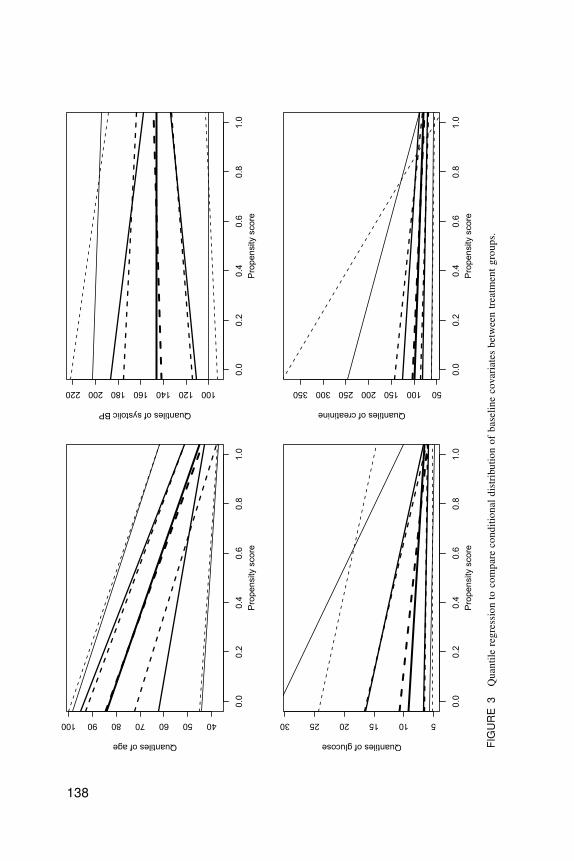
Figure 3 displays the graphical balance diagnostics based on quantile regres-

sion for age, systolic blood pressure, creatinine, and glucose. The relationship

between the quantiles of the baseline variable and the propensity score in treated

participants is described using the five solid lines, whereas the relationship be-

tween the quantiles of the baseline variable and the propensity score in untreated

participants is described using the five dashed lines. In examining Figure 3, one

notes that the distribution of each of the four baseline covariates is approximately

similar between treatment groups across the range of the propensity score.

However, there was some evidence of differences in the 95th percentile of the

FIG

UR

E2

Co

mp

arin

gd

istr

ibu

tio

no

fco

nti

nu

ou

sco

var

iate

sin

inv

erse

pro

bab

ilit

yo

ftr

eatm

ent

wei

gh

ted

sam

ple

.

137

FIG

UR

E3

Qu

anti

lere

gre

ssio

nto

com

par

eco

nd

itio

nal

dis

trib

uti

on

of

bas

elin

eco

var

iate

sb

etw

een

trea

tmen

tg

rou

ps.

138


conditional distributions between treated and untreated participants for three of

the four continuous covariates.

Based on the results of the balance diagnostics described in the preceding

sections, we were satisfied that our specification of the propensity score was

adequate. Having satisfied ourselves that the propensity score model was ade-

quately specified, we proceeded to estimate the effect of treatment on outcomes

using the four different propensity score methods.

Estimated Treatment Effects

Propensity score matching. The matched sample consisted of 646 matched

pairs. In this matched sample, 91 treated participants and 103 untreated partici-

pants died within 3 years of hospital discharge. The probabilities of death within

3 years of discharge were 0.141 (91/646) and 0.159 (103/646) for treated and

untreated participants, respectively. The absolute reduction in the probability of

3-year mortality was 0.0185 (95% confidence interval [�0.018, 0.055]). There

was no significant difference in the probability of 3-year mortality between

treatment groups .p D :3173/. The NNT, the reciprocal of the absolute risk

reduction, was 54. Thus, one would need to provide in-patient counseling to 54

smokers in order to avoid one death within 3 years of hospital discharge. The

relative risk of death in treated participants compared with untreated participants

was 91/103 D 0.88 (95% confidence interval: [0.69, 1.13]). Thus, in-patient

smoking cessation counseling reduced the risk of 3-year mortality by 12%.

However, the relative risk was not statistically significantly different from unity

.p D :3176/. Thus, there was no evidence that the provision of smoking

cessation counseling reduced the risk of death in current smokers within 3 years

of hospital discharge.

The left panel of Figure 4 depicts the Kaplan-Meier survival curves in treated

and untreated participants in the propensity score matched sample. The two

survival curves were not significantly different from one another .p D :2486/.

Using a Cox proportional hazards model, the estimated hazard ratio was 0.874

(95% confidence interval: [0.672, 1.136]). Thus, provision of smoking cessation

counseling prior to hospital discharge reduced the hazard of subsequent death

by 12.6%. However, this effect was not statistically different from the null effect

.p D :3130/.

Stratification on the propensity score. The probability of 3-year mortality

in participants not receiving in-patient smoking cessation counseling was 0.37,

0.16, 0.10, 0.05, and 0.05 in the first through fifth strata of the propensity score,

respectively. The probability of 3-year mortality in participants receiving in-

patient smoking cessation counseling was 0.25, 0.14, 0.09, 0.04, and 0.04 in

the first through fifth strata, respectively. Thus, the absolute reduction in 3-year

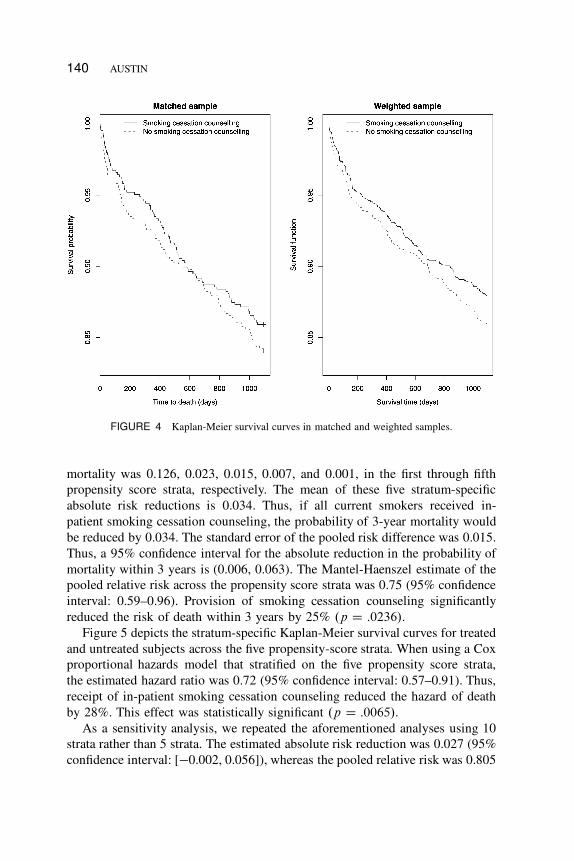
140 AUSTIN

FIGURE 4 Kaplan-Meier survival curves in matched and weighted samples.

mortality was 0.126, 0.023, 0.015, 0.007, and 0.001, in the first through fifth

propensity score strata, respectively. The mean of these five stratum-specific

absolute risk reductions is 0.034. Thus, if all current smokers received in-

patient smoking cessation counseling, the probability of 3-year mortality would

be reduced by 0.034. The standard error of the pooled risk difference was 0.015.

Thus, a 95% confidence interval for the absolute reduction in the probability of

mortality within 3 years is (0.006, 0.063). The Mantel-Haenszel estimate of the

pooled relative risk across the propensity score strata was 0.75 (95% confidence

interval: 0.59–0.96). Provision of smoking cessation counseling significantly

reduced the risk of death within 3 years by 25% .p D :0236/.

Figure 5 depicts the stratum-specific Kaplan-Meier survival curves for treated

and untreated subjects across the five propensity-score strata. When using a Cox

proportional hazards model that stratified on the five propensity score strata,

the estimated hazard ratio was 0.72 (95% confidence interval: 0.57–0.91). Thus,

receipt of in-patient smoking cessation counseling reduced the hazard of death

by 28%. This effect was statistically significant .p D :0065/.

As a sensitivity analysis, we repeated the aforementioned analyses using 10

strata rather than 5 strata. The estimated absolute risk reduction was 0.027 (95%

confidence interval: [�0.002, 0.056]), whereas the pooled relative risk was 0.805

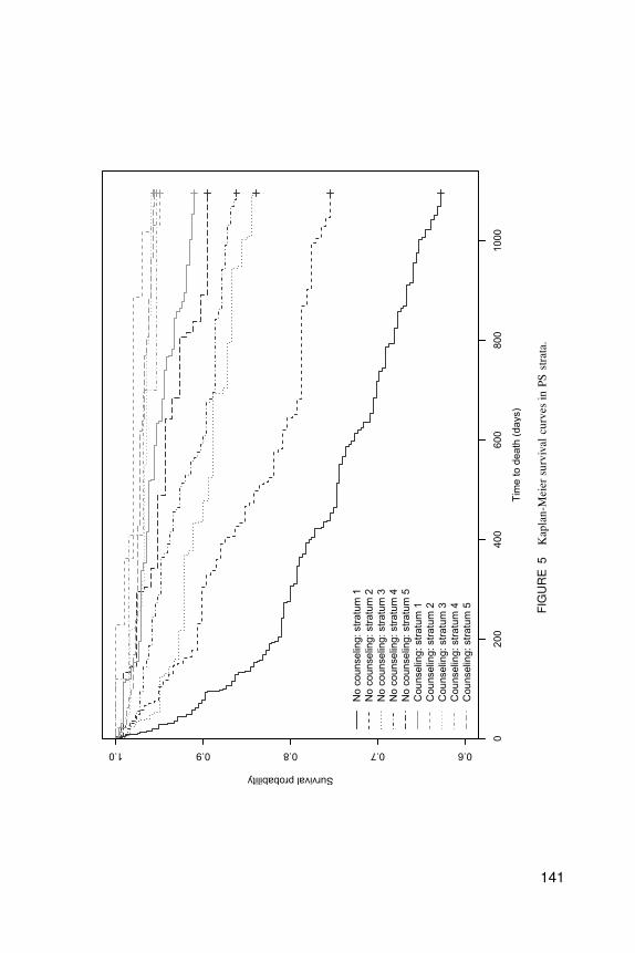
FIG

UR

E5

Kap

lan

-Mei

ersu

rviv

alcu

rves

inP

Sst

rata

.

141

142 AUSTIN

(95% confidence interval: 0.628–1.031). For time to death, the estimated hazard

ratio was 0.775 (95% confidence interval: 0.608–0.989). Thus, smoking cessation

counseling decreased the hazard of death by 22.5% .p D :04/.

Propensity score weighting. Using the first weighted estimate, counseling

reduced the probability of death within 3 years by 0.020 (95% confidence

interval: �0.008 to 0.047), which was not statistically significantly different from

0 .p D :1558/. The O�DR estimate of the absolute reduction in the probability

of mortality due to counseling was 0.025 (95% confidence interval: �0.002 to

0.052). Counseling did not reduce the probability of mortality within 3 years of

discharge .p D :0689/.

Using the first weighted estimator, the relative risk of death within 3 years

in treated patients compared with untreated patients was 0.86 (95% confidence

interval: 0.66–1.10). Using the doubly robust estimator, the relative risk was

0.82 (95% confidence interval: 0.66–1.03).

Using logistic regression in the weighted sample, the resultant odds ratio was

0.84 (95% confidence interval: 0.63–1.11). When the logistic regression model

was modified by adjusting for the 33 variables in Table 1, the estimated odds ratio

was attenuated to 0.98 (95% confidence interval: 0.95–1.00). In neither case was

the estimated odds ratio statistically significantly different from 1 (p D :2193

and .0998, respectively).

When a Cox proportional hazards model was used in the weighted sample,

the estimated hazard ratio for counseling was 0.850 (95% confidence interval:

0.655 to 1.102). Thus, counseling did not reduce the hazard of subsequent death

.p D :2203/. The right panel of Figure 4 displays the estimates of the Kaplan-

Meier survival curves in the sample weighted by the inverse probability of

treatment. One observes that in-patient smoking cessation counseling improved

survival postdischarge. At 3 years, the probability of death was 0.880 and 0.860

in those who did and did not receive counseling, respectively. The absolute

reduction in the probability of death within 3 years due to smoking cessation

counseling was 0.020. However, there was no evidence that the two survival

curves were different from one another .p D :2107/.

Covariate adjustment using the propensity score. When we used logis-

tic regression to regress the odds of survival to 3 years on an indicator variable

for treatment status and the propensity score, one inferred that receipt of in-

patient smoking cessation counseling reduced the odds of death within 3 years of

discharge by 20.8% (odds ratio: 0.792; 95% confidence interval: 0.600–1.046).

Similarly, treatment reduced the hazard of postdischarge mortality by 20.2%

(hazard ratio: 0.798; 95% confidence interval: 0.624–1.022). Neither the odds

ratio nor the hazard ratio were statistical significantly different from the null

treatment effect (p D :100 and .074, respectively). As noted in the Methods


section, use of these approaches is discouraged as they have been shown to lead

to biased estimation of odds ratios and hazard ratios.

When using the method based on that described by Imbens (2004), we

estimated that the probability of death within 3 years if all participants were

untreated was 0.144, whereas the probability of death if all participants were

treated was 0.121. Thus, treatment reduced the population probability of death

within 3 years by 0.023 (95% confidence interval was [�0.005, 0.052]). Sim-

ilarly, the relative risk was 0.84 (16% relative reduction in the probability of

death within 3 years of hospital discharge; 95% confidence interval: 0.68–1.04).

Thus, using covariate adjustment using the propensity score, neither the effect

of counseling on the absolute or relative reduction in the probability of mortality

was statistically significant from the null effect.

Regression adjustment. When logistic regression was used to regress an

indicator variable denoting survival to 3 years postdischarge on an indicator

variable denoting receipt of smoking cessation counseling and the 33 baseline

covariates listed in Table 1, the adjusted odds ratio for smoking cessation coun-

seling was 0.73 (95% confidence interval: 0.54–0.98). Thus, smoking cessation

counseling reduced the odds of mortality .p D :0371/. When the logistic

regression model was modified by using restricted cubic smoothing splines to

model the relationship between continuous baseline covariates and the log-odds

of mortality, the resultant odds ratio for counseling was 0.77 (95% confidence

interval: 0.56–1.05). Thus, smoking cessation counseling did not significantly

reduce the odds of mortality .p D :0942/.

When we used a Cox proportional hazards model to regress survival time

on treatment status and the 33 baseline covariates listed in Table 1, the ad-

justed hazard ratio for smoking cessation counseling was 0.72 (95% confidence

interval: 0.57–0.92). Thus, smoking cessation counseling reduced the hazard

of postdischarge mortality .p D :0080/. When we modified the Cox propor-

tional hazards model by using restricted cubic smoothing splines to model

the relationship between continuous baseline covariates and the log-hazard of

mortality, the resultant hazard ratio for counseling was 0.78 (95% confidence

interval: 0.61–0.99). Thus, counseling significantly reduced the hazard of death

.p D :0441/.

DISCUSSION

In this case study and tutorial on propensity score methods, we have illustrated

the use of different propensity score methods for estimating treatment effects

when using observational data. Several observations merit highlighting and dis-

cussion.

144 AUSTIN

First, we highlight that specifying the propensity score model was an iterative

process that involved several iterations of model specification and assessing the

balance of measured baseline covariates between treated and untreated partici-

pants in the propensity score matched sample. In this case study, we required

three steps before we were satisfied that the propensity score model had been

adequately specified. Balance assessment plays a critical role in any propensity

score analysis.

Second, different propensity score methods eliminated systematic differences

between treated and untreated participants to differing degrees. Propensity score

matching and inverse probability of treatment weighting using the propensity

score reduced systematic differences between treated and untreated participants

to a greater extent than did stratification on the propensity score or covariate

adjustment using the propensity score. These observations are similar to prior

empirical observations and to the results of Monte Carlo simulations (Austin,

2009c).

Third, when outcomes were binary, propensity score methods allowed esti-

mation of absolute risk reductions (or differences in proportions) and relative

risks. In contrast, conventional logistic regression only allowed estimation of

odds ratios. Many authors have suggested that relative risks and risk differences

are preferable to odds ratios for quantifying the magnitude of treatment effects

(Sackett, 1996; Sinclair & Bracken, 1994). The reader is referred elsewhere

for a more detailed discussion of propensity score methods for estimating risk

differences and relative risks (Austin, 2008d, 2010e; Austin & Laupacis, 2011).

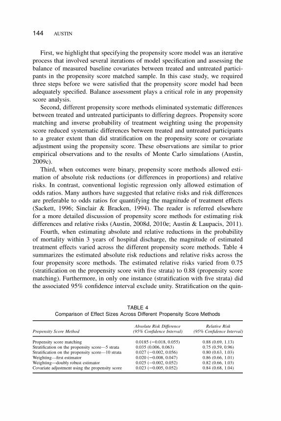
Fourth, when estimating absolute and relative reductions in the probability

of mortality within 3 years of hospital discharge, the magnitude of estimated

treatment effects varied across the different propensity score methods. Table 4

summarizes the estimated absolute risk reductions and relative risks across the

four propensity score methods. The estimated relative risks varied from 0.75

(stratification on the propensity score with five strata) to 0.88 (propensity score

matching). Furthermore, in only one instance (stratification with five strata) did

the associated 95% confidence interval exclude unity. Stratification on the quin-

TABLE 4

Comparison of Effect Sizes Across Different Propensity Score Methods

Propensity Score Method

Absolute Risk Difference

(95% Confidence Interval)

Relative Risk

(95% Confidence Interval)

Propensity score matching 0.0185 (�0.018, 0.055) 0.88 (0.69, 1.13)

Stratification on the propensity score—5 strata 0.035 (0.006, 0.063) 0.75 (0.59, 0.96)

Stratification on the propensity score—10 strata 0.027 (�0.002, 0.056) 0.80 (0.63, 1.03)

Weighting—first estimator 0.020 (�0.008, 0.047) 0.86 (0.66, 1.01)

Weighting—doubly robust estimator 0.025 (�0.002, 0.052) 0.82 (0.66, 1.03)

Covariate adjustment using the propensity score 0.023 (�0.005, 0.052) 0.84 (0.68, 1.04)


tiles of the propensity score removed less of the systematic differences between

treated and untreated participants than did matching or weighting using the

propensity score. Thus, the greater effect size obtained using stratification may

reflect a greater amount of residual bias. In our comparison of treated and un-

treated participants in the original sample, we observed that treated participants

tended to be younger and healthier than untreated participants. Furthermore,

they were more likely to receive discharge prescriptions for medications that

reduce cardiac mortality and morbidity. Thus, some of the difference between the

stratified estimate and those obtained using weighting or matching may reflect

persistent residual differences between treated and untreated participants with

the treated participants being healthier than the untreated participants. Similarly,

when estimating absolute risk reductions, the greatest reduction in mortality was

observed when stratification was used, whereas the smallest absolute reduction

was observed when matching was used. As with relative risks, stratification was

the only propensity score method that resulted in a 95% confidence interval for

the absolute risk reduction that excluded the null value.

Fifth, we highlight that propensity score matching allows one to estimate the

ATT, whereas the other three methods allow one to estimate the ATE (Imbens,

2004, although we note that the other methods can be adapted to estimate the

ATT as well). The latter three methods allow one to estimate the effect on

average mortality in the population if one shifted the entire population from

receiving no counseling to receiving smoking cessation counseling. Because

of how matching was done, the matching estimator is estimating the effect

of smoking cessation counseling in those participants who ultimately did not

receive counseling. We have already noted that participants who did not receive

smoking cessation counseling tended to be older and sicker than patients who

received counseling. Thus, the populations to which each estimate applies are

qualitatively and quantitatively different from one another. In comparing the

two panels of Figure 4, one should note that the probability of survival to 3

years is different in the untreated population (matched analysis) compared with

survival in the overall population if all participants were untreated (weighted

analysis). Complicating the interpretation of the matched estimator is the fact that

of those patients who did not receive in-patient smoking cessation counseling,

only 86% were successfully matched to a patient who did receive smoking

cessation counseling. Ideally, each participant who did not receive counseling

would be matched to a participant who received counseling. Then, the estimated

treatment effect would apply to the population of participants who did not receive

counseling. However, we have noted that, of those participants who did not

receive counseling, unmatched participants were systematically different from

those who were matched. In particular, unmatched participants were substantially

older. Due to incomplete matching, it is not clear how to describe the population

to which the matched estimator applies. Incomplete matching appears to occur

146 AUSTIN

frequently in applied applications, complicating the interpretation of the matched

estimator. Applied investigators need to decide which of the ATE or the ATT

is more meaningful in their research context. In the context of smoking cessa-

tion counseling offered to patients hospitalized with an AMI, the choice may

depend in part on the intensity of counseling and the degree to which patients’

commitment is required.

Sixth, we contrast the different odds ratios that were obtained using different

methods. In the sample weighted by the inverse probability of treatment, we

obtained two odds ratios: 0.84 and 0.98. The first was obtained by regressing

survival on treatment status, whereas the second was obtained after additional ad-

justment for baseline covariates. Neither odds ratio was statistically significantly

different from one .p > :09/. In contrast, conventional logistic regression in the

original unweighted sample resulted in an odds ratio of 0.73 (this was attenuated

to 0.77 when cubic smoothing splines were used to model the relationship

between continuous baseline covariates and the log-odds of mortality). The first

two odds ratios are estimates of the marginal odds ratio for the reduction in

mortality due to counseling, whereas the latter two odds ratios are estimates of

the conditional odds ratio (Rosenbaum, 2005). Differences between these two

sets of estimates reflect the fact that propensity score methods allow for esti-

mation of marginal treatment effects, whereas regression adjustment allows for

estimation of conditional treatment effects (Rosenbaum, 2005). For odds ratios,

marginal and conditional effects do not coincide (Gail, Wieand, & Piantadosi,

1984; Greenland, 1987).

Seventh, we highlight that there are well-developed methods for assessing

the similarity of treated and untreated participants conditional on the propensity

score. These methods allow one to assess whether the propensity score model

has been adequately specified. Having removed or reduced systematic differences

between treatment groups, one can then directly compare outcomes in the resul-

tant matched, stratified, or weighted sample. In contrast, when using regression

adjustment it is more difficult to assess whether the regression model relating

outcomes to treatment and baseline covariates has been correctly specified. In

our initial conventional logistic regression model, the odds ratio for counseling

was 0.73 .p D :0371/. However, this was attenuated to 0.77 .p D :0942/ when

cubic smoothing splines were used to model the relationship between continuous

baseline variables and the log-odds of mortality. However, uncertainty persists

as to whether this second model had been adequately specified.

Eighth, we remind the reader that propensity score methods only allow

one to account for measured baseline variables. Estimates using each of the

estimates of treatment effect may be susceptible to bias due to unmeasured

confounding variables. The reader is referred elsewhere for an illustration of

this (Austin, Mamdani, Stukel, Anderson, & Tu, 2005). Rosenbaum and Rubin

(1983) described sensitivity analyses to assess the sensitivity of the study conclu-


sions to unmeasured covariates when propensity score methods are used. These

sensitivity analyses allow one to assess how strongly an unmeasured confounder

would have to be associated with treatment selection in order for a previously

statistically significant treatment effect to become statistically nonsignificant if

the unmeasured confounder had been accounted for. However, in our case study,

the large majority of estimated effects were not statistically significant. Thus,

we did not employ these sensitivity analyses in this case study.

Ninth, we highlight that the question of whether providing smoking cessation

counseling reduces postdischarge mortality in AMI patients is a complex clinical

question Readers are referred elsewhere for an examination of this clinical

question (Van Spall, Chong, & Tu, 2007). The analyses presented in the current

case study were merely intended to illustrate the use of different statistical

methods and were not intended to address this clinical question. However, to

underline the importance of the clinical question, we note that a prior study found

that approximately 31% of patients who were discharged alive from the hospital

with a diagnosis of AMI were current smokers at the time of the infarction,

whereas 36% were former smokers (Rea et al., 2002). A meta-analysis of 12

cohort studies found that smoking cessation following AMI reduced the odds of

subsequent mortality by 46% (Wilson, Gibson, Willan, & Cook, 2000). It is im-

portant to note that this mortality benefit was consistent across a range of factors.

Given the large number of patients hospitalized with acute myocardial infarction,

the high prevalence of current smokers among these patients, the high mortality

rate in this patient population, and the potential benefit of smoking cessation

in these patients, it is critical that effective means of successfully encouraging

smoking cessation be developed. A systematic review of 33 randomized and

quasi-randomized controlled trials found that smoking cessation counseling in

hospitalized smokers increased the odds of smoking cessation at 6 and 12

months by 65% if the counseling began during hospitalization and included

supportive contacts for more than 1 month after hospital discharge (Rigotti,

Munafo, & Stead, 2008). However, interventions with less postdischarge contact

were not found to be effective. In the context of patients hospitalized with AMI,

a randomized controlled trial found that bedside smoking cessation counseling

followed by seven telephone calls over the first 6 months after discharge had

a substantial effect on smoking cessation 1 year after discharge (Dornelas,

Sampson, Gray, Waters, & Thompson, 2000). In an analysis of a multicenter

registry of patients hospitalized with an AMI, a multivariable analysis found

that, although individual smoking cessation counseling did not influence of the

odds of smoking cessation, being treated at a facility that offered an in-patient

smoking cessation program increased the odds of smoking cessation (Dawood

et al., 2008). Finally, a meta-analysis found that, when comparing different

health care providers, smoking cessation was most effective when provided by

physicians (Gorin & Heck, 2004).

148 AUSTIN

In summary, we have illustrated the appropriate steps in conducting analyses

using different propensity score methods. Increased use of these methods may

allow for more transparent estimation of causal treatment effects using observa-

tional data.

ACKNOWLEDGMENTS

This study was supported by the Institute for Clinical Evaluative Sciences

(ICES), which is funded by an annual grant from the Ontario Ministry of

Health and Long-Term Care (MOHLTC). The opinions, results, and conclusions

reported in this article are those of the authors and are independent of the funding

sources. No endorsement by ICES or the Ontario MOHLTC is intended or should

be inferred. Peter C. Austin is supported in part by a Career Investigator award

from the Heart and Stroke Foundation of Ontario. This study was supported

in part by an operating grant from the Canadian Institutes of Health Research

(CIHR; Funding Number MOP 86508). The EFFECT data used in the study

was funded by a CIHR Team Grant in Cardiovascular Outcomes Research.

REFERENCES

Agresti, A., & Min, Y. (2004). Effects and non-effects of paired identical observations in comparing

proportions with binary matched-pairs data. Statistics in Medicine, 23, 65–75.

Austin, P. C. (2007a). Propensity-score matching in the cardiovascular surgery literature from

2004 to 2006: A systematic review and suggestions for improvement. Journal of Thoracic and

Cardiovascular Surgery, 134, 1128–1135. doi:10.1016/j.jtcvs.2007.07.021

Austin, P. C. (2007b). The performance of different propensity score methods for estimating marginal

odds ratios. Statistics in Medicine, 26, 3078–3094. doi:10.1002/sim.2781

Austin, P. C. (2008a). A critical appraisal of propensity score matching in the medical literature

from 1996 to 2003. Statistics in Medicine, 27, 2037–2049. doi:10.1002/sim.3150

Austin, P. C. (2008b). A report card on propensity-score matching in the cardiology literature from

2004 to 2006: Results of a systematic review. Circulation: Cardiovascular Quality and Outcomes,

1, 62–67. doi:10.1161/CIRCOUTCOMES.108.790634

Austin, P. C. (2008c). Goodness-of-fit diagnostics for the propensity score model when estimating

treatment effects using covariate adjustment with the propensity score. Pharmacoepidemiology

and Drug Safety, 17, 1202–1217. doi:10.1002/pds.1673

Austin, P. C. (2008d). The performance of different propensity score methods for estimating relative

risks. Journal of Clinical Epidemiology, 61, 537–545. doi:10.1016/j.jclinepi.2007.07.011

Austin, P. C. (2009a). Using the standardized difference to compare the prevalence of a binary

variable between two groups in observational research. Communications in Statistics Simulation

and Computation, 38, 1228–1234. doi:10.1080/03610910902859574

Austin, P. C. (2009b). Balance diagnostics for comparing the distribution of baseline covariates

between treatment groups in propensity-score matched samples. Statistics in Medicine, 28, 3083–

3107. doi:10.1002/sim.3697


Austin, P. C. (2009c). The relative ability of different propensity-score methods to balance measured

covariates between treated and untreated subjects in observational studies. Medical Decision

Making, 29, 661–677. doi:10.1177/0272989X09341755

Austin, P. C. (2009d). Type I error rates, coverage of confidence intervals, and variance estimation

in propensity-score matched analyses. The International Journal of Biostatistics, 5, Article 13.

doi:10.2202/1557-4679.1146

Austin, P. C. (2010a). Optimal caliper widths for propensity-score matching when estimating differ-

ences in means and differences in proportions in observational studies. Pharmaceutical Statistics.

doi:10.1002/pst.433

Austin, P. C. (2010b). Absolute risk reductions, relative risks, relative risk reductions, and numbers

needed to treat can be obtained from a logistic regression model. Journal of Clinical Epidemiology,

63, 2–6. doi:10.1016/j.jclinepi.2008.11.004

Austin, P. C. (2010c). Absolute risk reductions and numbers needed to treat can be obtained from

adjusted survival models for time-to-event outcomes. Journal of Clinical Epidemiology, 63, 46–55.

doi:10.1016/j.jclinepi.2009.03.012

Austin, P. C. (2010d). The performance of different propensity score methods for estimating differ-

ence in proportions (risk differences or absolute risk reductions) in observational studies. Statistics

in Medicine, 29, 2137–2148. doi:10.1002/sim.3854

Austin, P. C., & Laupacis, A. (2011). A tutorial on methods to estimating clinically and policy-

meaningful measures of treatment effects in prospective observational studies: A review. Interna-

tional Journal of Biostatistics, 7, article 6. doi:10.2202/1557-4769.1285

Austin, P. C. (in press-a). Using the propensity score to estimate treatment effects in observational

studies: Designing observational studies to look like randomized experiments. Multivariate Be-

havioral Research.

Austin, P. C. (in press-b). Comparing paired vs. non-paired statistical methods of analyses when

making inferences about absolute risk infections in propensity-score matched samples. Statistics

in Medicine. doi:10.1002/sim.4200.

Austin, P. C., Grootendorst, P., & Anderson, G. M. (2007). A comparison of the ability of different

propensity score models to balance measured variables between treated and untreated subjects: A

Monte Carlo study. Statistics in Medicine, 26, 734–753. doi:10.1002/sim.2580

Austin, P. C., Grootendorst, P., Normand S. L. T., & Anderson, G. M. (2007). Conditioning on

the propensity score can result in biased estimation of common measures of treatment effect: A

Monte Carlo study. Statistics in Medicine, 26, 754–768. doi:10.1002/sim.2618

Austin, P. C., & Mamdani M. M. (2006). A comparison of propensity score methods: A case-study

estimating the effectiveness of post-AMI statin use. Statistics in Medicine, 25, 2084–2106. doi:

10.1002/sim.2328

Austin, P. C., Mamdani, M. M., Stukel, T. A., Anderson, G. M., & Tu, J. V. (2005). The use of the

propensity score for estimating treatment effects: Administrative versus clinical data. Statistics in

Medicine, 24, 1563–1578. doi:10.1002/sim.2053

Austin, P. C., Tu, J. V., Daly, P. A., & Alter, D. A. (2005). The use of quantile regression in

health care research: A case study examining gender differences in the delivery of thrombolysis.

Statistics in Medicine, 24, 791–816. doi:10.1002/sim.1851

Breslow, N. E., & Day, N. E. (1987). Statistical methods in cancer research: Vol. 2. The design and

analysis of cohort studies. Lyon, France: International Agency for Research on Cancer.

Cummings, P., McKnight, B., & Greenland, S. (2003). Matched cohort methods for injury research.

Epidemiologic Reviews, 25, 43–50.

Dawood, N., Vaccarino, V., Reid, K. J., Spertus, J. A., Hamid, N., Parashar, S., & PREMIER Registry

Investigators. (2008). Predictors of smoking cessation after a myocardial infarction: The role of

institutional smoking cessation programs in improving success. Archives of Internal Medicine,

168, 1961–1967.

150 AUSTIN

Dornelas, E. A., Sampson, R. A., Gray, J. F., Waters, D., & Thompson, P. D. (2000). A randomized

controlled trial of smoking cessation counseling after myocardial infarction. Preventive Medicine,

30, 261–268.

Efron, B., & Tibshirani, R. J. (1993). An introduction to the bootstrap. New York, NY: Chapman &

Hall.

Flury, B. K., & Riedwyl, H. (1986). Standard distance in univariate and multivariate analysis. The

American Statistician, 40, 249–251.

Gail, M. H., Wieand, S., & Piantadosi, S. (1984). Biased estimates of treatment effect in randomized

experiments with nonlinear regressions and omitted covariates. Biometrika, 7, 431–444.

Gorin, S. S., & Heck, J. E. (2004). Meta-analysis of the efficacy of tobacco counseling by health

care providers. Cancer Epidemiology, Biomarkers and Prevention, 13, 2012–2022.

Greenland, S. (1987). Interpretation and choice of effect measures in epidemiologic analyses.

American Journal of Epidemiology, 125, 761–768.

Harrell, F. E., Jr. (2001). Regression modeling strategies (with applications to linear models, logistic

regression, and survival analysis). New York, NY: Springer-Verlag.

Harrington, D. (2005). Linear rank tests in survival analysis. In P. Armitage & T. Colton (Eds.),

Encyclopedia of biostatistics (2nd ed., pp. 2802–2812). New York, NY: Wiley.

Ho, D. E., Imai, K., King, G., & Stuart, E. A. (2007). Matching as nonparametric preprocessing for

reducing model dependence in parametric causal inference. Political Analysis, 15, 199–236.

Imai, K., King, G., & Stuart, E. A. (2008). Misunderstandings between experimentalists and ob-

servationalists about causal inference. Journal of the Royal Statistical Society, Series A, 171,

481–501.

Imbens, G. W. (2004). Nonparametric estimation of average treatment effects under exogeneity: A

review. The Review of Economics and Statistics, 86, 4–29.

Joffe, M. M., Ten Have, T. R., Feldman, H. I., & Kimmel, S. E. (2004). Model selection, confounder

control, and marginal structural models: Review and new applications. The American Statistician,

58, 272–279.

Klein, J. P., & Moeschberger, M. L. (1997). Survival analysis: Techniques for censored and truncated

data. New York, NY: Springer-Verlag.

Lin, D. Y., & Wei, L. J. (1989). The robust inference for the proportional hazards model. Journal

of the American Statistical Association, 84, 1074–1078.

Lunceford, J. K., & Davidian, M. (2004). Stratification and weighting via the propensity score in

estimation of causal treatment effects: A comparative study. Statistics in Medicine, 23, 2937–2960.

Rea, T. D., Heckbert, S. R., Kaplan, R. C., Smith, N. L., Lemaitre, R. N., & Psaty B. M. (2002).

Smoking status and risk for recurrent coronary events after myocardial infarction. Annals of

Internal Medicine, 137, 494–500.

Rigotti, N. A., Munafo, M. R., & Stead, L. F. (2008). Smoking cessation interventions for hospital-

ized smokers: A systematic review. Archives of Internal Medicine, 168, 1950–1960.

Rosenbaum, P. R. (2005). Propensity score. In P. Armitage & T. Colton (Eds.), Encyclopedia of

biostatistics (2nd ed., pp. 4267–4272). Chichester, England: Wiley.

Rosenbaum, P. R., & Rubin, D. B. (1983). Assessing sensitivity to an unobserved binary covariate

in an observational study with binary outcome. The Journal of the Royal Statistical Society, B,

45, 212–218.

Rosenbaum, P. R., & Rubin, D. B. (1984). Reducing bias in observational studies using subclassi-

fication on the propensity score. Journal of the American Statistical Association, 79, 516–524.

Rosenbaum, P. R., & Rubin, D. B. (1985). Constructing a control group using multivariate matched

sampling methods that incorporate the propensity score. The American Statistician, 39, 33–38.

Sackett, D. L. (1996, September/October). Down with odds ratios! Evidence-Based Medicine, pp.

164–166.

Sinclair, J. C., & Bracken, M. B. (1994). Clinically useful measures of effect in binary analyses of

randomized trials. Journal of Clinical Epidemiology, 47, 881–889.


Tu, J. V., Donovan, L. R., Lee, D. S., Austin, P. C., Ko, D. T., Wang, J. T., & Newman, A. M.

(2004). Quality of cardiac care in Ontario: Phase 1 (Report No. 1). Toronto, Ontario, Canada:

Institute for Clinical Evaluative Sciences.

Tu, J. V., Donovan, L. R., Lee, D. S., Wang, J. T., Austin, P. C., Alter, D. A., & Ko, D. T. (2009).

Effectiveness of public report cards for improving the quality of cardiac care: The Enhanced

Feedback For Effective Cardiac Treatment (EFFECT) study. Journal of the American Medical

Association, 302, 2330–2337.

Van Spall, H. G. C., Chong, A., & Tu, J. V. (2007). Inpatient smoking-cessation counseling and

all-cause mortality in patients with acute myocardial infarction. American Heart Journal, 154,

213–220.

Weitzen, S., Lapane, K. L., Toledano, A. Y., Hume, A. L., & Mor, V. (2005). Weaknesses of

goodness-of-fit tests for evaluating propensity score models: the case of the omitted confounder.

Pharmacoepidemiology and Drug Safety, 14, 227–238.

Wilson, K., Gibson, N., Willan, A., & Cook, D. (2000). Effect of smoking cessation on mortality

after myocardial infarction: Meta-analysis of cohort studies. Archives of Internal Medicine, 160,

939–944.

Xie, J., & Liu, C. (2005). Adjusted Kaplan-Meier estimator and log-rank test with inverse probability

of treatment weighting for survival data. Statistics in Medicine, 24, 3089–3110.

a tutorial and case study in propensity score analysis: …hal.case.edu/~robrien/austin11a tutorial...

Documents