1

A Total Cost of Ownership Model for High Temperature PEM Fuel Cells in Combined Heat and Power Applications

Max Wei, Timothy Lipman1, Ahmad Mayyas1, Shuk Han Chan2, David Gosselin2, Hanna Breunig, Thomas McKone

Lawrence Berkeley National Laboratory (LBNL) 1 Cyclotron Road MS 90R-4000 Berkeley, California, 94706 Phone: (510) 486-5220 E-mail: mwei@lbl.gov

1University of California, Berkeley, Transportation Sustainability Research Center, Berkeley, California 2University of California, Berkeley, Laboratory for Manufacturing and Sustainability, Department of Mechanical Engineering, Berkeley, California

Revision 1

Environmental Energy Technologies Division October 2014

This work was supported by the U.S. Department of Energy under Lawrence Berkeley National Laboratory Contract No. DE-AC02-05CH11231

ERNEST ORLANDO LAWRENCE BERKELEY NATIONAL LABORATORY

2

DISCLAIMER

This document was prepared as an account of work sponsored by the United States Government. While this document is believed to contain correct information, neither the United States Government nor any agency thereof, nor The Regents of the University of California, nor any of their employees, makes any warranty, express or implied, or assumes any legal responsibility for the accuracy, completeness, or usefulness of any information, apparatus, product, or process disclosed, or represents that its use would not infringe privately owned rights. Reference herein to any specific commercial product, process, or service by its trade name, trademark, manufacturer, or otherwise, does not necessarily constitute or imply its endorsement, recommendation, or favoring by the United States Government or any agency thereof, or The Regents of the University of California. The views and opinions of authors expressed herein do not necessarily state or reflect those of the United States Government or any agency thereof, or The Regents of the University of California. Ernest Orlando Lawrence Berkeley National Laboratory is an equal opportunity employer.

3

Acknowledgements

The authors gratefully acknowledge the U.S. Department of Energy, Office of Energy Efficiency and Renewable Energy (EERE) Fuel Cells Technologies Office (FCT) for their funding and support of this work. The authors would like to express their sincere thanks to Bob Sandbank from Eurotech, Mark Miller from Coating Tech Services, Geoff Melicharek and Nicole Fenton from ConQuip, Emory DeCastro from Advent Technologies, Dominic Gervasio from University of Arizona, Douglas Wheeler from DJW Technology, Hans Aage Hjuler from Danish Power Systems, Tequilla Harris from Georgia Institute of Technology, Charles Tanzola from Innoventures, Owen Hopkins from Entegris, Paul Dyer from Zoltec, Andrew DeMartini from Doosan Fuel Cell America, Inc. and Charleen Chang from Richest Group (Shanghai, China) for their assistance and valuable inputs.

4

Table of Contents Executive Summary................................................................................................................................ 6

Table of Abbreviations and Nomenclature ................................................................................... 8

1. Introduction ............................................................................................................................... 10

1.1. System Design .................................................................................................................................... 11

1.2. Functional Specifications ............................................................................................................... 12

2. DFMA Manufacturing Cost Analysis .................................................................................. 14

2.1. Polybenzimidazol (PBI) based membranes ................................................................................ 14

2.1.1. Process Flow of PBI-Based membrane .......................................................................... 16

2.1.2. Casting Process Parameters ................................................................................................ 19

2.1.3. Cost Model Results for PBI-based membrane ............................................................ 21

2.2. Gas Diffusion Electrode (GDE) ......................................................................................................... 24

2.2.1. Preparation of the GDEs impregnated with phosphoric acid ............................ 24

2.2.2 Cost Model Results for Gas Diffusion Electrode ......................................................... 25

2.3. Membrane Electrode Assembly (MEA) Frame .......................................................................... 27

2.3.1. MEA Frame Cost Model Results ......................................................................................... 28

2.4. Separator Plates .................................................................................................................................... 30

2.4.1. Cost Model Results for the Separator Plate ................................................................. 35

2.4.2. Sensitivity Analysis for HAP ................................................................................................ 39

2.4.3. Simplified Half Plates .............................................................................................................. 41

2.5. Stack Assembly Process ...................................................................................................................... 42

2.5.1. Stack Assembly Results .......................................................................................................... 42

2.6. Sensitivity Analysis .............................................................................................................................. 43

3. Balance of Plant and Fuel Processor Cost ........................................................................ 46

3.1 BOP Costing Approach ......................................................................................................................... 46

4. Fuel Cell System Direct Manufacturing Costing Results .......................................... 50

4.1. HT PEM Fuel Cell System Costing Results ................................................................................... 50

4.2. Comparison between HT PEM and LT PEM Fuel Cell Systems ........................................... 55

5 Total Cost of Ownership Modeling of CHP Fuel Cell Systems ............................... 59

5.1. Use-phase Model ................................................................................................................................... 59

5.1.1. Use-phase model results ....................................................................................................... 60

5.2. Life Cycle Impact Assessment (LCIA) Modeling ........................................................................ 64

5.3. Total Cost of Ownership Modeling Results ................................................................................. 67

6. Conclusions ...................................................................................................................................... 72

5

References ............................................................................................................................................. 74

Appendix A: Costing Approach and Considerations ...................................................... 77

A.1. DFMA Costing Model Approach ...................................................................................................... 78

A.2. Non-Product Costs ............................................................................................................................... 81

A.3. Manufacturing Cost Analysis - Shared Parameters ................................................................. 82

A.4. Factory model ........................................................................................................................................ 84

A.5. Yield Considerations ............................................................................................................................ 84

A.6. Initial Tool Sizing .................................................................................................................................. 84

A.7. Time-frame for Cost Analysis........................................................................................................... 85

Appendix B: DFMA Manufacturing Cost Analysis ............................................................. 86

B.1. Polybenzimidazol88 (PBI) based membranes .......................................................................... 86

Appendix C: Balance of Plant Cost and Total System Cost Results ....................... 109

Appendix D: Total Cost of Ownership Modeling of CHP Fuel Cell Systems ...... 125

6

Executive Summary A total cost of ownership model is described for emerging applications in stationary fuel cell systems, specifically high temperature proton exchange membrane (HT PEM) systems for use in combined heat and power applications from 1 to 250 kilowatts-electric (kWe1). The total cost of ownership framework expands the direct manufacturing cost modeling framework of other studies to include operational costs, life-cycle impact assessment of possible ancillary financial benefits during operation and at end-of-life, including credits for reduced emissions of global warming gases, such as carbon dioxide (CO2) and methane (CH4), reductions in environmental and health externalities, and end-of-life recycling. System designs and functional specifications for HT PEM fuel cell systems for co-generation applications were developed across the range of system power levels above. Detailed, design-for-manufacturing-and-assembly2 (DFMATM) analysis was utilized to estimate the direct manufacturing costs for key fuel cell stack components. The costs of the fuel processor subsystem are also based on an earlier DFMATM analysis by Strategic Analysis (James, 2012). Since HT PEM fuel cell systems were not available for inspection, balance of plant components relied on the inspection of currently installed LT PEM and phosphoric acid fuel cell (PAFC) systems for balance of plant subsystem components, and these were adopted for HT PEM technology. Note that there are few HT PEM FC systems currently in operation due to a variety of stack reliability and system design issues (Brooks, 2014). This work assumes that these stack issues and system design issues can be resolved with further research and development activities. The manufacturing costs presented here thus represent the authors’ best estimates for longer-lifetime HT PEM technology but may in fact be an underestimate of true manufacturing costs if additional more expensive design features required for robust CHP system operation are not captured here. Fuel cell stack costs and overall system costs have a strong dependence on the annual production volume. Overall system costs including corporate markups and installation costs are about $3900/kWe for 10kWe CHP systems at an annual production volume of 50,000 systems per year, and about $2400/kWe for 100kWe CHP systems at 50,000 systems per year. Bottom-up cost analyses show that the development of high throughput, automated processes achieving high yield is a key success factor in achieving lower fuel cell stack costs. At high production volume, material costs dominate the cost of fuel cell stack manufacturing. For CHP systems at low power, the fuel processing subsystem is the largest cost contributor to total non-stack costs. At high power, the electrical power subsystem is the dominant cost contributor to non-stack costs. Cost reduction opportunities for BOP components are expected to be available through both greater standardization of fuel cell subsystem parts and optimized design. Compared to the authors’ recent report on LT PEM CHP systems (Wei et al., 2014), HT PEM CHP direct system costs are about 15% higher at low annual production volumes (100 x 10kWe systems per year) to 30% higher at high volumes (50,000 x 100kWe systems per year). Current cost estimates for HT PEM CHP systems are more costly than LT PEM CHP systems costs due to three main factors: (1) lower current density and higher cell areal size; (2) more complex plate design and expensive plate process; and (3) higher catalyst loading. 1 In this report, units of kWe stand for net kW electrical power unless otherwise noted. 2 DFMA is a registered trademark of Boothroyd, Dewhurst, Inc. and is the combination of the design of manufacturing processes and design of assembly processes for ease of manufacturing and assembly and cost reduction.

7

Life-cycle or use-phase modeling and life cycle impact assessment (LCIA) were carried out for a several building types (e.g., small hotel and hospitals) in several locations in the United States (Phoenix, AZ, Chicago, IL, Minneapolis, MN, New York City, NY, Houston, TX, and San Diego, CA). For example, assuming capital costs corresponding to 100MWe of annual production (or 10,000 x 10kWe systems), installing a 10kWe CHP fuel cell system in a small hotel would reduce the effective cost of electricity ($/kWhe)) by 14-26% from heating fuel savings; 2-16% in savings from carbon credits from greenhouse gas reduction; and 1-20% savings from societal health and environmental externalities. The amount of these savings are dependent on several factors such as the cost of natural gas, utility tariff structure, amount of waste heat utilization, carbon intensity of displaced electricity, and carbon price. Including heating credit, global warming reduction credits and health and environmental impacts can reduce the levelized cost of electricity for HT PEM FC systems by up to 58% in small hotels and up to 65% in hospitals studied in Chicago. This project cost study considers both externalities and ancillary financial benefits, and thus provides a comprehensive picture of fuel cell system benefits, consistent with a policy and incentive environment that increasingly values these ancillary benefits. The project provides important modeling results that should aid a broad range of policy makers in assessing the integrated costs and benefits of fuel cell systems versus other distributed generation technologies.

8

Table of Abbreviations and Nomenclature AC alternating current APEEP Air Pollution Emission Experiments and Policy Analysis Model AEF average emission factor BIP bipolar plate BOL beginning of life BOM bill of material BOP balance of plant BPP bipolar plate BU backup BUP backup power CEM continuous emissions monitoring system CCM catalyst coated membrane CEUS California Commercial End-use Survey CHP combined heat and power CO carbon monoxide DC direct current DER CAM Distributed Energy Resources Customer Adoption Model DFMA Design for Manufacturing and Assembly DG distributed generation DHW domestic hot water DI de-ionizing DOE U.S. Department of Energy DTI DTI Energy Inc. EOL end of life EPA Environmental Protection Agency ePTFE expanded polytetrafluoroethylene FC fuel cell FCS fuel cell system FEP fluorinated ethylene propylene FMEA failure modes and effect analysis FP fuel processor GDL gas diffusion layer GHG greenhouse gas GIS geographic information system GREET Argonne National Laboratory’s Greenhouse Gases, Regulated Emissions, and Energy

Use in Transportation model GWP global warming potential G&A general and administrative expense HDPE high density polyethylene HHV higher heating value HMI human machine interface HT high temperature IM injection molding IR infrared kWe kilowatts of electricity kWhe kilowatt-hours of electricity LBNL Lawrence-Berkeley National Laboratory LCA life cycle assessment

9

LCC life cycle cost modeling LCIA life cycle impact assessment modeling LHV lower heating value LMAS Laboratory for Manufacturing and Assembly LSCF lanthanum-strontium-cobalt-ferrite LT low temperature L-AEF localized average emission factor MCO manganese cobalt oxide MEA membrane electrode assembly MEF marginal emission factor Min minutes MRO Midwest Reliability Organization NERC North American Electric Reliability Corporation NG natural gas Ni-Co nickel cobalt Nm3 normal cubic meters NOx nitrogen oxides NREL National Renewable Energy Laboratory NSTF nanostructured thin film NSPC Northern State Power Company O&M operation and maintenance PBI Polybenzimidazol PEN polyethylene naphthalate PEM proton exchange membrane PFSA perfluorinated sulfonic acid PM Particulate matter PNNL Pacific Northwest National Laboratory ppmv parts per million (by volume) PROX preferential oxidation PTFE polytetrafluoroethylene Pt/Co/Mn platinum-cobalt-manganese PVD physical vapor deposition R&D research and development expense SMR steam methane reformer SOFC solid oxide fuel cell SR steam reforming TCO total cost of ownership model UTC United Technologies Corporation VOC volatile organic compound WECC Western Electricity Coordinating Council WGS water gas shift

10

1. Introduction High temperature (HT) proton exchange membrane (PEM) fuel cells (FC) are a promising fuel cell technology that has several advantages compared to low temperature PEM fuel cells (LT PEM). Typical HT PEM FC operating temperatures are in the range of 100-200°C and these higher operating temperatures offer higher waste heat temperature for combined heat and power applications, provide greater tolerance to fuel impurities, and allow for simpler balance of system design. The status of HT PEM technology is that it is in the pre-commercial, development stage. A recent deployment pilot of several 5kW HT PEM CHP units in the U.S. resulted in many early failures due to both stack issues (e.g., plate cracking, phosphoric acid loss, and sealing issues) and system design issues (Brooks 2014), and there are few companies working on the technology in the U.S. There is interest worldwide, however, and companies such as Eisenhuth and Danish Power Systems in Europe are working on HT PEM stack bipolar plates and membrane electrode assemblies (MEA), respectively. The CISTEM project3 in Europe has the objective of developing a modular HT PEM CHP system with system sizes up to 100kWe. This work assumes that these stack issues and system design issues can be resolved with further research and development activities. The manufacturing costs presented thus represent the authors’ best estimates for longer-lifetime HT PEM technology. In particular, a more complex plate design with a separator layer is adopted for better control of phosphoric acid within the MEA and a longer stack lifetime. These cost estimates may however be an underestimate of true manufacturing costs if additional more expensive design features are required for robust CHP system operation. This chapter discusses stack and system designs and other functional specifications of the HT PEM fuel cell systems that utilize reformate fuel with natural gas as the primary fuel source. Cost modeling of the HT PEM fuel cell stack modules is presented in Chapter 2 using a design for manufacturing and assembly (DFMA) approach. Costing models are developed in a way that emphasizes materials and manufacturing costs, potential recycling and reuse of some scrapped materials. Non-fuel processor balance of the plant cost analysis, in contrast, relies primarily on purchased components, while fuel processor costs utilize earlier bottom-up costing from Strategic Analysis. Overall, cost results show the effect of production volume and economies of the scale on the final cost of HT PEM fuel cell systems. Chapters 3 and 4 describe the balance of plant components and costs, and total direct and installed system costs, respectively. The bottom-up cost DFMA cost estimates for the fuel cell stack are a key input for total system costs. Modeling the “total cost of ownership” (TCO) of fuel cell systems involves considering capital costs, fuel costs, operating costs, maintenance costs, “end of life” valuation of recoverable components and/or materials, valuation of externalities and comparisons with a baseline or other comparison scenarios. Including both “private” and “total social costs” (externalities) in TCO analysis allows examination of the extent to which they diverge and un-priced impacts of this technology’s implementation. These divergences can create market imperfections that lead to sub-optimal social 3 CISTEM is an acronym for “Construction of Improved HT-PEM MEAs and Stacks for Long Term Stable Module CHP Units.” More information on this project can be found at http://www.project-cistem.eu/index.php?id=1, accessed on October 15, 2014.

11

outcomes, but in ways that are potentially correctible with appropriate public policies (e.g., applying prices to air and water discharges that create pollution). Chapter 5 presents the analysis approach and results for HT PEM life-cycle or use-phase costs for two building types (small hotels and hospitals) in six U.S. cities (New York City, Chicago, Minneapolis, Houston, Phoenix, and San Diego) with FC capital costs derived from the system cost analysis in Chapter 4. Externality valuation associated with HT PEM CHP system operation is provided based on the research team’s earlier modeling (Wei et al., 2014). This includes greenhouse gases and health and environmental externalities. The final section of this report presents TCO modeling of HT PEM CHP systems including use-phase costs, heating fuel savings, and externality valuations. Much of the analysis approach here has been adopted by the authors’ earlier report on LT PEM total cost of ownership analysis for CHP and backup power systems (Wei et al., 2014). This earlier report on LT PEM TCO analysis will be referenced throughout the discussion that follows.

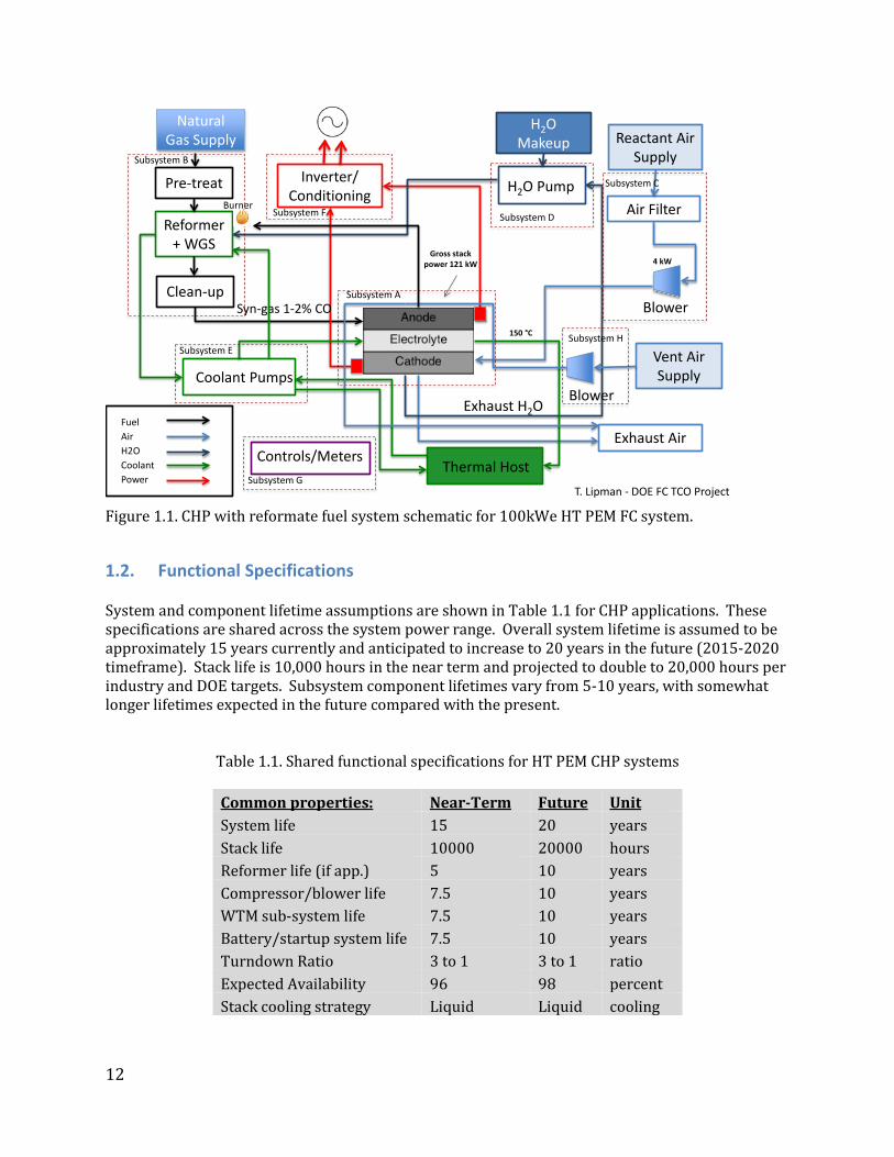
1.1. System Design Figure 1 shows the system design for a 100kWe HT PEM CHP system with reformate fuel. For bill of materials and component itemization, the system design has been divided into the following subsystems: stack, fuel processing, air supply, water makeup, coolant subsystem, power conditioning, controls and meters, and ventilation air supply. Note that compared to a LT PEM CHP system design, the HT PEM system has the following design simplifications for the balance of plant: no membrane humidification required, no air-slip at the anode due to greater CO tolerance in the incoming fuel stream, and less CO clean up requirement for input fuel in the fuel processing subsystem.

12

Figure 1.1. CHP with reformate fuel system schematic for 100kWe HT PEM FC system.

1.2. Functional Specifications System and component lifetime assumptions are shown in Table 1.1 for CHP applications. These specifications are shared across the system power range. Overall system lifetime is assumed to be approximately 15 years currently and anticipated to increase to 20 years in the future (2015-2020 timeframe). Stack life is 10,000 hours in the near term and projected to double to 20,000 hours per industry and DOE targets. Subsystem component lifetimes vary from 5-10 years, with somewhat longer lifetimes expected in the future compared with the present.

Table 1.1. Shared functional specifications for HT PEM CHP systems

Common properties: Near-Term Future Unit System life 15 20 years Stack life 10000 20000 hours Reformer life (if app.) 5 10 years Compressor/blower life 7.5 10 years WTM sub-system life 7.5 10 years Battery/startup system life 7.5 10 years Turndown Ratio 3 to 1 3 to 1 ratio Expected Availability 96 98 percent Stack cooling strategy Liquid Liquid cooling

Fuel

H2OCoolantPower

Air

Inverter/Conditioning

Coolant Pumps

T. Lipman - DOE FC TCO Project

Syn-gas 1-2% CO

Air Filter

Reactant Air Supply

Exhaust Air

Blower

H2O Makeup

Exhaust H2O

Subsystem A

Subsystem C

Subsystem D

Subsystem E

Subsystem F

Controls/MetersSubsystem G

H2O Pump

Thermal Host

Vent Air Supply

Blower

Subsystem H

Reformer+ WGS

Natural Gas Supply

Pre-treat

Clean-up

Subsystem B

Burner

4 kWGross stack

power 121 kW

150 °C

13

Functional specifications by system size are shown in Table 1.2 for 1-250kWe system sizes. The current density of 0.23 A/cm2 is based on an Advent Technologies specifications sheet. This necessitates about double the plate area of the corresponding LT PEM fuel cell size (Wei, et al. 2014). The physical size and weight is also about twice that of the LT PEM case. Waste heat range is expected to be in the 120-200°C range though the thermal efficiency will be highly site-specific and the values shown in Table 1.2 are upper estimates. Table 1.2. Functional specifications for HT PEM CHP systems with reformate fuel

Fuel utilization of 95% requires a fuel after-burner with fuel processor subsystem. GDE coated area is assumed to be 64% of total plate area (464/725 cm2) to account for manifolds and cooling channels, but this may be a conservative estimate, and single cell active area is assumed to be 9% lower than GDE coated area. Parasitic losses are assumed to be10% lower for HT PEM compared to LT PEM case due to simplification of system design. Precious metal catalyst loading is assumed to be 0.7mg Pt per cm2. (Chapter 2 has further details on catalyst loading).

Fuel Cell Size 1 kW 10 kW 50 kW 100 kW 250 kW

Unique Properties: Units:System Gross system power 1.28 12.6 62.6 121 305.8 kW

Net system power 1 10 50 100 250.0 kW (AC)Physical size 0.7x0.45x0.5 2.4x1.8x1.0 2.9x4.2x1.8 2.9x4.2x3.6 5.8x4.6x4.5 m3

Physical weight 110 1100 7040 14080 35200.0 kgElectrical output 110V AC 480V AC 480V AC 480V AC 480V AC Volts AC or DCDC/AC inverter effic. 93% 93% 93% 93% 90.0 %

Peak ramp rate 0.12 1.20 6.00 0.372 0.9 kW/sec - size depWaste heat grade 150 C. 150 150 150 150.0 Temp. °CReformer efficiency 75 75% 75% 75% 0.8 %Fuel utilization % (first pass) 80% 80% 80% 80% 0.8 %Fuel utilization % (overall) 95% 95% 95% 95% 1.0 %Fuel input power (LHV) 3.53 35 173 335 844.7 kWStack voltage effic. 51% 51% 51% 51% 51% % LHVGross system electr. effic. 36% 36% 36% 36% 36% % LHV

also see fn-> Avg. system net electr. effic. 28% 29% 29% 30% 30% % LHV Thermal efficiency 52% 52% 53% 53% 55% % LHVTotal efficiency 80% 81% 82% 83% 85% Elect.+thermal (%)

Stack stack power 1.28 6.3 7.83 8.08 8.0 kWtotal plate area 725 725 725 725 725 cm2

GDL coated area 468 468 468 464 464 cm2

single cell active area 426 426 426 423 423 cm2

gross cell inactive area 41 41 41 41 41 %cell amps 97.4 96.0 95.6 95 94.7 Acurrent density 0.23 0.23 0.22 0.23 0.22 A/cm2

reference voltage 0.625 0.625 0.625 0.625 0.625 Vpower density 0.143 0.141 0.140 0.141 0.140 W/cm2

single cell power 60.9 60.0 59.7 59 59.2 Wcells per stack 21 105 131 136 136 cellspercent active cells 100 100 100 100 100 %stacks per system 1 2 8 15 38 stacks

Addt'l ParasitCompressor/blower 0.05 0.5 3 4 10.0 kWOther paras. loads 0.153 1.35 5.85 9.72 27.0 kWParasitic loss 0.20 1.85 8.85 13.72 37.0 kW

14

2. DFMA Manufacturing Cost Analysis DFMA stack module cost analysis modeling assumptions and results are presented in this chapter for HT PEM fuel cell stacks designed for combined heat and power applications. Stack modules include the PBI membrane, gas diffusion electrode (GDE), MEA frame/seal, separator plates, and stack assembly module. The following sections discuss each stack module’s process flows, bill of materials, and cost analyses. A description of the costing analysis can be found in the earlier LT PEM report and is described in the Appendix. Each stack module has its own yield assumptions, but those modules that are based on mature manufacturing process or that are similar to LT PEM process modules have higher yield numbers. These higher yield numbers are based on manufacturing learning-by-doing over the past decades in making these components and due to the level of automation and quality control that is associated with established manufacturing processes such as compression molding of composite plates or the stamping process for metal plates.

2.1. Polybenzimidazol (PBI) based membranes Great progress in fuel cell system performance has been achieved using polymeric membranes based on perfluorosulfonic acid (PFSA) such as Nafion® for conventional low temperature PEM fuel cells that operate at temperature below 80°C. However, these polymeric membranes are not suitable at relatively higher temperatures (>120°C) and hence are not suitable for high temperature PEM fuel cells (see Table 2.1 below). Table 2.1 also shows other membrane materials that can be used in high temperature PEM fuel cells. Polybenzimidazol (PBI) based membranes are among the best performing group of membranes that can work efficiently at temperatures exceeding 120°C, not only because of their stability at high temperatures, but also because they have very good proton conductivity above 100°C. PBI membranes do not require membrane humidification which is another important factor to consider in PEM fuel cell system design. PBI-based high-temperature polymer-electrolyte membranes offer many advantages over other membrane technologies. Benefits include higher resistance to impurities than LT PEM (most notably carbon monoxide), faster electrochemical kinetics, and relatively simpler water and thermal management systems due to operational temperatures above 120°C (Schmidt and Baurmeister, 2008). Membrane bill of materials (BOM) was determined based on several studies (e.g. Xiao, et al., 2003; Xiao, 2005; Scanlon and Benicewicz, 2004) and tabulated in Tables 2.2-2.3. Table 2.2 summarizes first generation monomers used in making PBI membrane along with potential suppliers (Xiao, 2003); however, this early generation of PBI-based membranes were improved significantly through additions of some stronger and heat resistant monomers like phthalic acids in the second generation of PBI-based membranes (see Table 2.3).

15

Table 2.1 Some of the membrane technologies used in high temperature PEM fuel cells (Adopted from Bose et al. 2011) Types of membrane Operational

temperature (°C) Relative humidity (%)

Proton conductivity (S/cm)

Functionalized PDMS (APP 414) 130 100 0.072 SPES/BPO4 composite 120 # 0.038 SPFEK-SiO2-HPMC hybrid membrane

120 50 0.0198

Disulfonated poly(arylene ether sulfone)/ZrP composite

130 100 0.13

Sulfonated polyimides 140 10-20 0.0005 160 5-12 0.002

Nafion/ZrSPP composite 110 50 ≥0.005 98 ≤0.05

PBI/ZrP composite 200 5 0.096 S-polyoxadiazole/mesoporous silica (MCM-41)

120 25 0.034

Krytox-Si-Nafion hybrid membrane

130 Ambient condition

1.72 X10-4

Nafion/sulfonated poly(phenylsilsesquioxane) (sPPSQ) nanocomposite

120 100 0.157

Nafion/silica (SBA-15) 140 10 8.52 X10-4

Heteropolyacid (HPA)/sulfonated BPSH composite

130 # 0.15

Polyimide Containing Pendant Sulfophenoxypropoxy Groups

120 100 1

poly(benzimidazole-co-aniline) 120 100 0.167 PPO/poly(styrene-b-vinylbenzylphosphonic acid)

140 100 0.28

Perfluorocyclobutyl containing polybenzimidazoles

140 Without humidification

0.12

polybenzimidazole (PBI) containing bulky basic benzimidazole side groups

180 Without humidification

0.16

Imidazole intercalated into sulfonated polyetherketone

membrane

120 Without humidification

0.01

200 Without humidification

0.02

16

Table 2.2 Bill of materials for first generation monomers Materials Suppliers Price Pyridine dicarboxylic acids (2,4-, 2,5-, 2,6- and 3,5- PDA)

Matrix Scientific Alpha Aeser Chemical Co.

$91 for 25 g $212for 500 g

3,3′,4,4′-Tetraaminobiphenyl (TAB)

European suppliers $500 per kg

Polyphosphoric acid (115%) Sigma-Aldrich Chemical Co. $60 for1 kg

Ammonia Hydroxide Sigma-Aldrich Chemical Co. $340 for 6X2.5L

Distilled water Sigma-Aldrich Chemical Co.

Phosphoric Acid (Conc. 85% for doping)

Duda Energy $40 per gallon

Dimethylacetamide (DMAc) Sigma-Aldrich Chemical Co. Alpha Aeser Chemical Co.

$542 for 6L $82.5 for 2.5L

Table 2.3 Bill of materials for second generation monomers Materials Suppliers Price

Isophthalic acid Alpha Aeser Chemical Co. $103 for 5kg

Terephthalic acid Alpha Aeser Chemical Co. $377 for 10kg

3,3′,4,4′-Tetraaminobiphenyl (TAB)

European suppliers $500 per kg

Polyphosphoric acid (115%) Sigma-Aldrich Chemical Co. $60 for1 kg

Ammonium Hydoroxide Sigma-Aldrich Chemical Co. $253.5 for 6 L

N,N-DiMethylAcetamide (DMAc)

Sigma-Aldrich Chemical Co. $62.2 for 2 L

2.1.1. Process Flow of PBI-Based membrane In the present model, we assumed that PBI-membrane is made via a casting process using slot-die coating machine (Harris et al., 2010a). The synthesis of PBI-membrane is performed by combining a pyridine dicarboxylic acid (PDA) and a tetraamine (TAB) with PPA in a suitable reaction vessel. The reaction temperature is controlled by a programmable temperature controller and a heat bath during a ramp-and-soak procedure. Typical polymerization temperatures are approximately190–220°C for 16–24 hours (Fig. 2.1a). Under the appropriate reaction conditions, high molecular weight PBI polymer is produced. This polymer solution is then filtrated to get a dry powder which is then ground up in order to directly cast into films as part of a deposited ink formulation (see next section for details). Upon exposure to ambient moisture, PPA is hydrolyzed to PA to yield highly PA-

17

doped PBI membranes (Fig. 2.1b). After casting, the hydrolysis of PPA to phosphoric acid by moisture from the surrounding environment induces a sol–gel transition. A transition from the polymer solution state to a gel state is observed during the hydrolysis as PPA (a good solvent for PBI) is converted in situ to PA (a poor solvent for PBI). This sol–gel transition (see Fig. 2.2) results in a mechanically stable, highly conductive membrane that is capable of operating at high temperature without humidification of feed gases (Seel et al., 2009). In this way acid-doping levels as high as 20–40 mol PA per repeat unit of PBI can be achieved with consequently high conductivity (over 0.2 S cm−1) yet with acceptable tensile strength (of up to 3.5MPa) (Li et al., 2009). In general, PBI membranes with higher PA-doping levels produce membranes with higher proton conductivities (Seel et al., 2009).

(a)

18

(b)

Figure 2.1. Process flow for making PBI-based membrane: a) mixing process; and b) subsequent process to make PBI/PPA powder that is used in the casting process

Figure 2.2. Hydrolysis and doping are made to get more stable membrane (Hydrolysis @T=25°C; RH=40±5%) (Seel et al., 2009)

Slot-die coating was assumed as a base-case for making PBI-based membrane (Harris et al., 2010). In this process, the polymeric materials are melted in the container and then fed through a regulator valve into the slot-die, which casts a precise amount of the molten material on the substrate film (see Fig. 2.3 for the schematic of this process). After that, the cast film is fed into the infrared dryer to get stable film which is then tested for pin holes, other defects, and thickness

19

uniformity. The final membrane is then doped in a phosphoric acid bath and wound into large spools and put on to a shelf for further curing at room temperature.

Figure 2.3. Schematic of the casting process and in situ quality control of PBI-based membrane

2.1.2. Casting Process Parameters The slot-die casting process of viscous materials requires certain conditions to ensure a final product with the desired quality. In order to get a reproducible, high-quality product, the casting of PBI membranes needs to be done with the proper conditions in an appropriate “coating window” to eliminate various types of defects such as dripping, air entrainment, and break lines4 that might be formed during the casting process (Bhamidipati et al., 2013). In the current study, we assumed the following parameters for the PBI casting process, determined through extensive research in the literature and previous studies:

• Membrane thickness: 100µm (4 mils) • Line speed: variable speed based on production volume (see Fig. 2.4). Line speed is a critical

point from both manufacturing and cost perspectives. Line speed is usually determined based on the processing requirements such as molten materials temperature, casting pressure, film thickness, viscosity, surface tension, dry content in the coating solution, desired dry thickness, etc. There may be limits to the attainable casting speeds but from a fundamental point of view the upper limit in coating speed is normally many meters per

4 Air entrainment and break lines are considered to be major defects encountered in cast PBI membranes during slot die coating, especially for high-viscosity solutions. At higher casting speeds, air bubbles get trapped between the substrate and the liquid film. In some cases, the air bubble is restricted to only a fraction of the total film thickness, while in other cases; the bubble extends all the way to the top of the film making a hole. Extending the coating speed beyond the air entrainment value may result in the formation of break lines. It has been found that as the coating speed increases, the originally straight contact line breaks into sawteeth structures and air bubbles eventually break up from the tip of these sawteeth (Bhamidipati et al., 2013).

20

second. In the current analysis we assumed actual line speeds based on experimental work done by Bhamidipati et al., (2013).

• Yield increases with production volume because of process learning and improved process control. Figure 2.5 shows yield values with the cast area. Low yield values were estimated for low production volumes and yield was assumed increase with increasing production volume due to learning-by-doing (e.g., a lower scrap rate of materials associated with set-up times).

Figure 2.4. Line speed as a function of annual cast area

Figure 2.5. Yield assumptions with the annual production volume (in m2)

0.0

0.1

0.2

0.3

0.4

0.5

0.6

0.7

1.E+00 1.E+01 1.E+02 1.E+03 1.E+04 1.E+05 1.E+06 1.E+07 1.E+08

Line

Spe

ed (m

/min

)

Annual Cast Area (m2)

Line Speed vs. Cast Area

y = 0.0139ln(x) + 0.7345 R² = 0.9882

70%

75%

80%

85%

90%

95%

100%

1.E+01 1.E+02 1.E+03 1.E+04 1.E+05 1.E+06 1.E+07 1.E+08

Yiel

d

Annual Cast Area (m2)

Yield vs. Cast Area

21

2.1.3. Cost Model Results for PBI-based membrane Cost analyses were made using the cost modeling approach and assumptions described in Appendix A. Total cost (in $/m2) for first and second generation polymeric materials are shown in Fig. 2.6a and Fig.2.6b, respectively. It is important to mention that there are no discounts in the cost of materials as a function of volume because these materials are assumed to be largely commodity-type materials. Final cost values are broken down into constituent factors to show capital, building, operational, labor and materials components as shown in Figures 2.7-2.8 for 10kWe and 100 kWe fuel cell systems, respectively. These figures show that cost is dominated by material cost at higher production volume. In contrast, cost is dominated by capital, scrap/waste and building cost at low production volumes as a direct result of under-utilization of resources and high scrap percentages. One solution to overcome the problem of the under-utilization of equipment resources is to use a smaller slot-die coater for example, but this analysis targeted higher volume production.

(a)

0

25

50

75

100

125

150

1.E+03 1.E+04 1.E+05 1.E+06 1.E+07 1.E+08

Cost

($/m

2 )

Annual Production Volume ( m2)

$20/m2

22

(b)

Figure 2.6. Membrane cost in ($/m2) for PBI-based PEM based on: (a) 1st generation materials (Xiao et al., 2003); and (b) 2nd generation materials (Xiao et al., 2005).

(a)

0

25

50

75

100

125

150

1.E+03 1.E+04 1.E+05 1.E+06 1.E+07 1.E+08

Cost

($/m

2 )

Annual Production Volume ( m2)

$15/m2

100 1,000 10,000 50,000Scrap/Waste 69.64 10.32 2.76 2.08Process: Building 29.63 2.96 0.30 0.24Process: Operational 23.69 4.53 1.07 0.98Process: Capital 228.78 22.88 2.29 1.81Direct Labor 7.13 6.64 2.43 1.16Direct Materials 13.89 13.89 13.89 13.89

050

100150200250300350400

Cost

($/m

2 )

Syst./yr

PBI Membrane for 10kW Stack

23

(b)

Figure 2.7. Cost breakdown for 10 kWe fuel cell system based on: (a) 1st generation materials and (b) 2nd generation materials

(a)

100 1,000 10,000 50,000Scrap/Waste 68.57 9.46 2.17 1.62Process: Building 29.63 2.96 0.30 0.24Process: Operational 23.69 4.53 1.07 0.98Process: Capital 228.78 22.88 2.29 1.81Direct Labor 7.13 6.64 2.43 1.16Direct Materials 8.64 8.64 8.64 8.64

050

100150200250300350400

Cost

($/m

2 )

(Syst./yr)

PBI Membrane for 10kW Stack

100 1,000 10,000 50,000Scrap/Waste 10.48 2.77 1.85 1.65Process: Building 3.05 0.30 0.21 0.18Process: Operational 4.59 1.08 0.96 0.97Process: Capital 23.55 2.36 1.62 1.34Direct Labor 6.64 2.43 1.30 1.15Direct Materials 13.89 13.89 13.89 13.89

0

25

50

75

Cost

($/m

2 )

Syst./yr

PBI Membrane for 100kW Stack

24

(b)

Figure 2.8. Cost breakdown for 100 kWe fuel cell system based on: (a) 1st generation materials and (b) 2nd generation materials

2.2. Gas Diffusion Electrode (GDE) In the high temperature PEM fuel cell, the catalyst is commonly deposited on the gas diffusion layer (GDL) and therefore is called the gas diffusion electrode (GDE). Although catalyst layers can be deposited on the membrane to form catalyst coated membrane (CCM) or on the gas diffusion layer, the second approach is favored for HT PEM because of lower cost, less labor requirements, and improved yield (Manhattan Project, 2011). 2.2.1. Preparation of the GDEs impregnated with phosphoric acid Fabrication of gas diffusion electrodes (GDEs) is made through slot-die coating process where slurries containing appropriate amounts of platinum catalysts or (slurries of platinum alloys). Slurries with the appropriate precious metal weight fractions were prepared by ultrasonic agitation for 20–40 min in a mixture of water and organic alcohols. These inks were coated onto the microporous layer of a GDL using slot-die coating technique followed by a drying step. The selection of catalyst material is governed by several factors such as cost, electrical activity and ability to withstand certain temperatures in some fuel cell applications. Initially, catalysts were made of platinum or other noble metals, as these materials have the ability to withstand the corrosive environment of the electrochemical cell. Later, these noble metals were dispersed over the surface of electrically conductive supporting materials (e.g. carbon black) to increase the surface area of the catalyst which in turn increased the number of reactive sites leading to improved efficiency of the cell. It was then discovered that certain alloys of noble metals exhibited increased catalytic activity, further increasing fuel cell efficiencies (Luczak, 1991). Some of these alloys are platinum-chromium and platinum vanadium. In addition, a ternary alloy catalyst containing platinum, cobalt and chromium was reported to have better efficiency by Luczak (1986)

100 1,000 10,000 50,000Scrap/Waste 9.63 2.19 1.46 1.32Process: Building 3.05 0.30 0.21 0.18Process: Operational 4.59 1.08 0.96 0.97Process: Capital 23.55 2.36 1.62 1.34Direct Labor 6.64 2.43 1.30 1.15Direct Materials 8.64 8.64 8.64 8.64

0

25

50

75

Cost

($/m

2 )

Syst./yr

PBI Membrane for 100kW Stack

25

in U.S. patent #4,613,582. The Pt/Cr/Co alloy loadings on the GDE are shown in Table 2.4 based on this patent.

The preparation of the platinum-chromium-cobalt alloy catalyst slurries to be deposited on the surface of the carbon paper was also adopted from the same UTC patent (U.S. patent #4,613,582). A brief description of the ink preparation method is provided in Appendix B.

Table 2.4. Platinum-Chromium-Cobalt alloy used in making ink slurry for GDE

Alloying Element

Composition (%)

Loading (mg/cm2)

Pt 79.8% 0.700 Cobalt 11.3% 0.099

Chromium 8.9% 0.078

Yield assumptions (per square-meter of GDE) are assumed to be between 90-99% depending on the annual production volume. Yield is assumed to improve with output volume in the slot-die coating process as a result of reduced amount of waste materials during set-up time and due to continuous learning that can be related to the annual production volumes in square meters. Note that “scrap” material is not discarded but the catalyst is recovered by shipping rejected material to a Pt recovery firm with the assumption that 90% of Pt material is recovered and the remaining 10% Pt is assumed to cover the cost of recovery.

2.2.2 Cost Model Results for Gas Diffusion Electrode A cost model was developed for GDE using the same approach as that described in Appendix A. Slot-die coating process is assumed to be the base catalyst deposition method in this study where the catalyst layer is deposited on carbon paper. Total cost (in $/m2) final GDE cost and carbon paper cost are shown in Fig. 2.9. It can be clearly seen that cost is decreasing with the production volume (expressed in m2 along x-axis) as a direct result of efficient use of equipment and materials. Cost breakdown is also shown in Fig. 2.10 for 10 kWe and 100 kWe fuel cell systems to emphasize the contribution of each cost components on the overall cost of the GDE. This figure shows that cost is greatly dominated by material cost at all production volumes (mainly Pt catalyst) followed by equipment cost as the next highest cost contributor.

26

Figure 2.9. Gas diffusion electrode (GDE) cost along with carbon paper cost in ($/m2) with annual production volumes

(a)

0

100

200

300

400

500

600

700

800

1.E+03 1.E+04 1.E+05 1.E+06 1.E+07 1.E+08

Cost

($/m

2 )

GDE Annual Coated Area (m2)

GDE cost ($/m2)

GDEGDL-Carbon Paper

100 1,000 10,000 50,000Scrap/Waste 23.23 -3.50 -9.63 -12.31Process: Building 23.50 2.37 0.24 0.10Process: Operational 12.49 1.37 0.24 0.16Process: Capital 105.85 10.70 1.08 0.44Direct Labor ($/kW) 0.35 0.34 0.34 0.34Direct Materials ($/kW) 515.82 329.52 278.62 254.78

0

200

400

600

800

Cost

($/m

2 )

Sys/yr

GDE Cost Breakdown (10kW System)

27

(b)

Figure 2.10. GDE cost breakdown for: (a) 10 kWe fuel cell system and (b) 100 kWe fuel cell system showing that cost is dominated by material cost (mainly the cost of platinum and carbon paper)

2.3. Membrane Electrode Assembly (MEA) Frame The manufacturing process of the MEA frame is very similar to that of the LT PEM process flow. Essentially, three input rolls (GDL cathode, GDL anode, and membrane) and the frame film are hot pressed together and punched to the desired area. However, the materials for the frame and backing are different due to physical property requirements and the elevated operating temperature of the HT PEM FC system. The materials modeled for the MEA seal and backing for the high temperature system are polyimide and Viton respectively compared to the low temperature system that utilized polyethylene naphthalate (PEN) and fluorinated ethylene propylene (FEP). An outline of the manufacturing process flow is shown in Figure 2.11 while material costs are shown in Table 2.5.

100 1,000 10,000 50,000Scrap/Waste -3.38 -9.57 -13.32 -15.63Process: Building 2.44 0.25 0.05 0.04Process: Operational 1.40 0.24 0.09 0.09Process: Capital 11.01 1.11 0.22 0.18Direct Labor ($/kW) 0.34 0.34 0.20 0.20Direct Materials ($/kW) 330.49 279.09 245.51 224.74

0

100

200

300

400

Cost

($/m

2 )

Sys/yr

GDE Cost Breakdown (100kW System)

28

Figure 2.11. MEA Frame process flow

Table 2.5. MEA seal and backing material cost and comparison to the LT PEM system

Layer Application Material Cost ($/m2)

MEA Seal HT PEM Polyimide 10.00 LT PEM PEN 5.00

Backing HT PEM Viton 7.60 LT PEM FEP 10.00

2.3.1. MEA Frame Cost Model Results Cost assumptions such as equipment cost, cycle time, process yield, line availability, set-up time, component design, and tooling footprint are identical to that of the LT PEM report and are documented in great detail (Wei et al., 2014). Figure 2.12 shows the cost breakdown of the MEA frame. At low production volumes, capital cost is the largest cost contributor. At high production volumes, direct materials and scrap dominate the overall frame cost. This is the expected trend since high line utilization at high volumes effectively distributes the initial capital cost over more parts. Material cost is therefore the cost driver at high volume. Scrap is large throughout all production volumes owing to the fact that all upstream work is lost in a defective framed MEA. In addition, it is seen that there is no reduction in scrap cost after reaching volumes of 10,000 system/yr for the 10kWe system and 1,000 systems/yr for the 100kWe system. This is owing to the assumption that a maximum yield (99.9%) is reached at lower production volumes to protect against losing a large portion of upstream value. The total frame cost at high production volume is about $3.45 per part. The numerical breakdown is shown in Table 2.6.

29

(a)

(b)

Figure 2.12. Cost Breakdown of MEA Frame a) 10kWe b) 100kWe

Table 2.6. Cost Breakdown of MEA Frame (a) 10kWe (b) 100kWe Volume (Systems/yr) 100 1,000 10,000 50,000 Direct Materials 1.31 1.31 1.31 1.31 Direct Labor 0.49 0.47 0.16 0.16 Process: Capital 6.68 0.66 0.30 0.26 Process: Operational 0.58 0.10 0.07 0.06 Process: Building 0.17 0.02 0.00 0.01 Scrap/Waste 6.47 2.09 1.65 1.65

Final Cost 15.70 4.65 3.50 3.45 (a)

0.00

2.00

4.00

6.00

8.00

10.00

12.00

14.00

16.00

18.00

100 1,000 10,000 50,000

$/Pa

rt

Systems/Yr

Scrap/WasteProcess: BuildingProcess: OperationalProcess: CapitalDirect LaborDirect Materials

0.00

0.50

1.00

1.50

2.00

2.50

3.00

3.50

4.00

4.50

5.00

100 1,000 10,000 50,000

$/Pa

rt

Systems/Yr

Scrap/WasteProcess: BuildingProcess: OperationalProcess: CapitalDirect Labor

30

Volume (Systems/yr) 100 1,000 10,000 50,000 Direct Materials 1.31 1.31 1.31 1.31 Direct Labor 0.47 0.16 0.16 0.16 Process: Capital 0.67 0.31 0.25 0.25 Process: Operational 0.10 0.07 0.06 0.06 Process: Building 0.02 0.01 0.01 0.01 Scrap/Waste 2.11 1.65 1.65 1.64

Final Cost 4.69 3.51 3.44 3.44 (b)

Figure 2.13 shows a comparison of frame cost of the HT PEM system to that of the low temperature PEM system. It is seen that the high temperature PEM frame is about $1.50 more expensive per MEA to manufacture than the low temperature PEM frame. This is due to the difference in material cost and larger frame footprint.

Figure 2.13. Comparison to MEA Frame for Low Temperature PEM

2.4. Separator Plates In the low temperature PEM fuel cell, a bipolar plate is used to supply reactants to each individual cell while also providing cooling channels. The cooling channels are created by adhering two half plates together. The low temperature half plate design is shown in Figure 2.14.

0

2

4

6

8

10

12

14

16

18

10000 100000 1000000 10000000 100000000 1E+09

$/Fr

ame

Frames/yr

High Temperature PEM

Low Temperature PEM

31

Figure 2.14. Bipolar Half Plate for Low Temperature PEM Fuel Cells

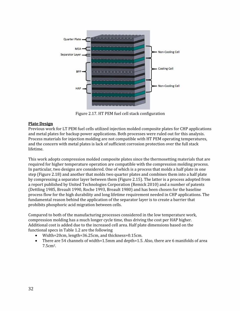
In a high temperature PEM fuel cell, cooling is not done in every cell because of the higher temperature and greater efficiency of heat dissipation. Typical HT PEM stacks have cooling cells every 5th to 8th cell (Kanuri, 2011), and this analysis assumes a low-end frequency of every 5th cell. Since cooling is needed every fifth cell, four of every five cells contain a single half plate (Figure 2.15) while one of every five cells contain a full bipolar plate (BPP) (Figure 2.16). In other words, compared to the low temperature case, there are 40% less half plates. This setup is shown in Figure 2.17. Note that in order to stay consistent with previous work on low temperature PEM fuel cells, a plate with reservoir channels on both sides is termed a half plate (HAP). Therefore, a plate with reservoir channels on one side and flat on the other is a referred to as a quarter plate.

Figure 2.15. Half Plate with Separator Layer

Figure 2.16. Plate Configuration for Cooling Cells

32

Figure 2.17. HT PEM fuel cell stack configuration

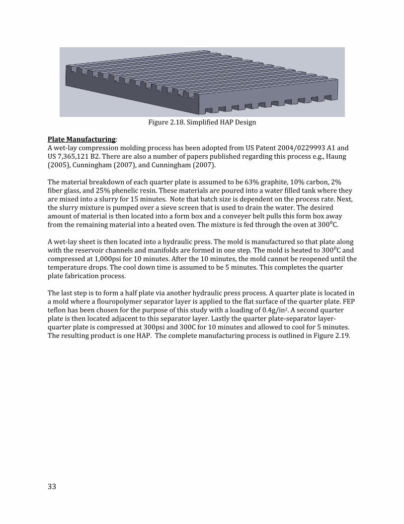
Plate Design Previous work for LT PEM fuel cells utilized injection molded composite plates for CHP applications and metal plates for backup power applications. Both processes were ruled out for this analysis. Process materials for injection molding are not compatible with HT PEM operating temperatures, and the concern with metal plates is lack of sufficient corrosion protection over the full stack lifetime. This work adopts compression molded composite plates since the thermosetting materials that are required for higher temperature operation are compatible with the compression molding process. In particular, two designs are considered. One of which is a process that molds a half plate in one step (Figure 2.18) and another that molds two quarter plates and combines them into a half plate by compressing a separator layer between them (Figure 2.15). The latter is a process adopted from a report published by United Technologies Corporation (Remick 2010) and a number of patents (Dettling 1985, Breault 1990, Roche 1993, Breault 1980) and has been chosen for the baseline process flow for the high durability and long lifetime requirement needed in CHP applications. The fundamental reason behind the application of the separator layer is to create a barrier that prohibits phosphoric acid migration between cells. Compared to both of the manufacturing processes considered in the low temperature work, compression molding has a much longer cycle time, thus driving the cost per HAP higher. Additional cost is added due to the increased cell area. Half plate dimensions based on the functional specs in Table 1.2 are the following

• Width=20cm, length=36.25cm, and thickness=0.15cm. • There are 54 channels of width=1.5mm and depth=1.5. Also, there are 6 manifolds of area

7.5cm2.

33

Figure 2.18. Simplified HAP Design

Plate Manufacturing: A wet-lay compression molding process has been adopted from US Patent 2004/0229993 A1 and US 7,365,121 B2. There are also a number of papers published regarding this process e.g., Haung (2005), Cunningham (2007), and Cunningham (2007). The material breakdown of each quarter plate is assumed to be 63% graphite, 10% carbon, 2% fiber glass, and 25% phenelic resin. These materials are poured into a water filled tank where they are mixed into a slurry for 15 minutes. Note that batch size is dependent on the process rate. Next, the slurry mixture is pumped over a sieve screen that is used to drain the water. The desired amount of material is then located into a form box and a conveyer belt pulls this form box away from the remaining material into a heated oven. The mixture is fed through the oven at 300⁰C. A wet-lay sheet is then located into a hydraulic press. The mold is manufactured so that plate along with the reservoir channels and manifolds are formed in one step. The mold is heated to 300⁰C and compressed at 1,000psi for 10 minutes. After the 10 minutes, the mold cannot be reopened until the temperature drops. The cool down time is assumed to be 5 minutes. This completes the quarter plate fabrication process. The last step is to form a half plate via another hydraulic press process. A quarter plate is located in a mold where a flouropolymer separator layer is applied to the flat surface of the quarter plate. FEP teflon has been chosen for the purpose of this study with a loading of 0.4g/in2. A second quarter plate is then located adjacent to this separator layer. Lastly the quarter plate-separator layer-quarter plate is compressed at 300psi and 300C for 10 minutes and allowed to cool for 5 minutes. The resulting product is one HAP. The complete manufacturing process is outlined in Figure 2.19.

34

Figure 2.19. Wet-Lay Compression Mold Diagram (Baird, 2004)

For the 100 ton manual press, process yield varies between 80% and 90% while line availability varies between 85% and 95%. For the automated presses, the same assumption for line availability is applied, however, the process yield is now capped at 99.5% due to the consistent nature of automated processing. Note that the low percentage assumption is taken at volumes less than 100,000 HAP/yr while the high percentage assumption is taken at volumes greater than 10,000,000 HAP/yr. Cost Analysis Assumptions: As annual production increases larger press sizes are used to make up for the large cycle time. The hydraulic press is the largest contributor to capital cost, which is also the largest contributor to the overall cost. The capital cost of each press is shown in Table 2.7. Note that the 100-ton press does not scale linearly with the other presses because it is assumed to be fully manual operated while the larger size presses are automatically operated with platen heaters included in the cost. Less cost intensive equipment is shown in Table 2.8.

Table 2.7. Cost estimate of Hydraulic Presses

Press Size (Ton) Cost ($) 500 500,000

1,000 1,000,000 2,000 2,000,000 5,000 5,000,000

10,000 10,000,000

35

Table 2.8. Equipment cost broken down by module ($)

Component Automatic Lines

Manual Lines

Stirrer 2500 50 Pulper 3700 2387 Pump 2500 200 Head Box 3000 100 Stirrer 2500 50 Sieve Screen 400 100 Continuous Roller

10000 500

Vacuum 5000 500 Oven 165000 500 Platen Heaters 0 500 Inspection 200000 0

2.4.1. Cost Model Results for the Separator Plate The HAP manufacturing process was analyzed in two phases. The first phase contains all steps upstream to a resulting quarter plate and the second phase contains all downstream steps. The cost curves associated with using different size hydraulic presses are shown in Figure 2.20 for both phases.

(a)

1

10

100

1,000

10,000

1.E+02 1.E+03 1.E+04 1.E+05 1.E+06 1.E+07 1.E+08

Cost

($/H

AP)

HAP/yr

100 Ton500 Ton1,000 Ton2,000 Ton5,000 Ton10,000 Ton

36

(b)

Figure 2.20. Cost vs. Production Volume for Selected Press Sizes (a) Phase 1 (b) Phase 2

The total cost of producing a HAP is derived by adding the optimum cost (lowest curve in Figures 2.20) for each phase at given production volumes. The resulting cost and optimum press size selections are shown in Table 2.9.

Table 2.9. Cost Results for HAP with Optimum Press Selection

Size Systems/yr $/Plate Primary

Press

Size

(Tons)

Secondary

Press Size

(Tons)

1 100 51.86 100 100 1000 24.25 1,000 100

10000 11.52 5,000 100 50000 8.21 10,000 2000

10 100 23.70 1,000 100 1000 11.30 5,000 100

10000 7.52 5,000 5000 50000 6.91 10,000 5000

50 100 16.83 1,000 100 1000 8.02 10,000 2000

10000 6.91 10,000 5000 50000 6.62 10,000 5000

1

10

100

1,000

1.E+02 1.E+03 1.E+04 1.E+05 1.E+06 1.E+07 1.E+08

Cost

($/H

AP)

HAP/yr

100 Ton

500 Ton

1,000 Ton

2,000 Ton

5,000 Ton

37

100 100 11.45 5,000 100 1000 7.64 5,000 5000

10000 6.73 10,000 5000 50000 6.62 10,000 5000

250 100 8.66 10,000 1000 1000 7.20 10,000 5000

10000 6.63 10,000 5000 50000 6.61 10,000 5000

The cost breakdown for the 10 and 100 kWe systems is shown in Figure 2.21. It is seen that capital cost is the largest contributor at all production volumes. This is due to the long cycle times associated with compression molding that cannot be avoided with this process. At low volumes (10kWe, 100 and 1,000 systems) it is seen that labor is the second largest cost contributor. This is a result of the need for manual labor to operate the 100-ton press in phase 2. As the production volume increase, the transition to automated equipment is made and operational cost then becomes the second largest cost contributor. The numerical breakdown is seen in Table 2.10. For the 10 kWe system, cost ranges from $23.70/HAP to $6.91/HAP while the 100kWe system yield cost from $11.45/HAP to $6.62/HAP.

(a)

0

5

10

15

20

25

100 1000 10000 50000

$/H

AP

Systems/yr

Scrap/WasteBuildingOperationalCapitalLaborDirect Materials

38

(b)

Figure 2.21. Cost Breakdown of HAP (a) 10kWe (b) 100kWe Table 2.10. Cost Breakdown of HAP (a) 10kWe (b) 100kWe

Volume 100 1,000 10,000 50,000 Direct Materials 0.63 0.53 0.52 0.52 Direct Labor 6.83 3.03 0.42 0.20 Process: Capital 12.46 4.84 3.93 3.59 Process: Operational 3.17 2.63 2.57 2.54 Process: Building 0.47 0.19 0.06 0.06 Scrap/Waste 0.13 0.10 0.02 0.00

Final Cost 23.70 11.30 7.52 6.91 (a)

Volume 100 1,000 10,000 50,000 Direct Materials 0.53 0.52 0.51 0.51 Direct Labor 3.04 0.43 0.18 0.17 Process: Capital 4.97 4.04 3.44 3.35 Process: Operational 2.63 2.58 2.53 2.53 Process: Building 0.19 0.06 0.06 0.06 Scrap/Waste 0.10 0.02 0.00 0.00

Final Cost 11.45 7.64 6.73 6.62 (b)

A direct comparison to the LT PEM plates cannot be made due to stack design difference. However, qualitatively speaking, the high temperature PEM plates are more expensive due to higher cycle times of compression molding compared to injection molding and the addition of a separator layer.

0

2

4

6

8

10

12

14

100 1000 10000 50000

$/H

AP

Systems/yr

Scrap/WasteBuildingOperationalCapitalLaborDirect Materials

39

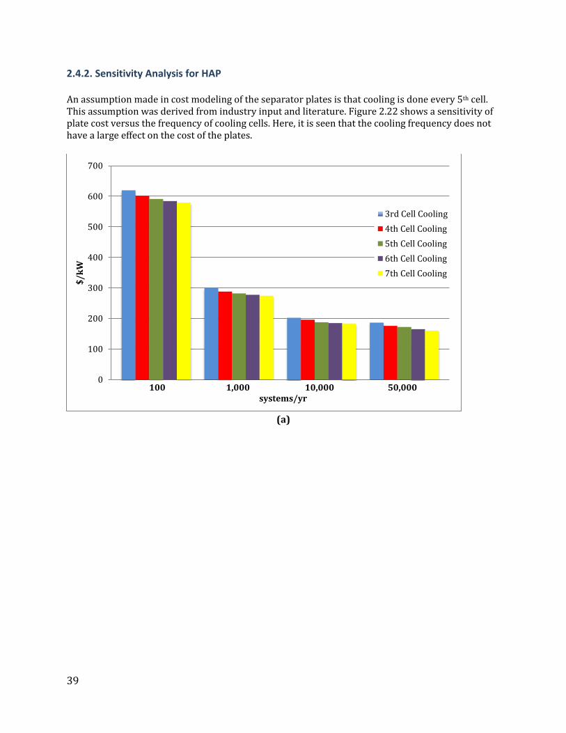
2.4.2. Sensitivity Analysis for HAP An assumption made in cost modeling of the separator plates is that cooling is done every 5th cell. This assumption was derived from industry input and literature. Figure 2.22 shows a sensitivity of plate cost versus the frequency of cooling cells. Here, it is seen that the cooling frequency does not have a large effect on the cost of the plates.

(a)

0

100

200

300

400

500

600

700

$/kW

100 1,000 10,000 50,000 systems/yr

3rd Cell Cooling4th Cell Cooling5th Cell Cooling6th Cell Cooling7th Cell Cooling

40

(b)

Figure 2.22. Sensitivity analysis of the cooling plate as a function of number of cooling plates per stack and annual production volume for: (a) 10kWe FC system; and (b) 100kWe FC system The pressure applied by the hydraulic press to the plates is another sensitivity that was analyzed. It is anticipated that this parameter has a large influence on the cost in the following way. A decrease in molding pressure leads to an increase in the number of plates that can be molded in a single pressing operation which leads to a decrease in the number of presses needed thus resulting in lower capital cost. Figure 2.23 shows this sensitivity. At high volumes the cost per half plate falls from $6.61 to $4.71 when molding pressure in decreased by 50%.

0

50

100

150

200

250

300

350$/

kW

100 1,000 10,000 50,000 systems/yr

3rd Cell Cooling4th Cell Cooling5th Cell Cooling6th Cell Cooling7th Cell Cooling

0.00

2.00

4.00

6.00

8.00

10.00

12.00

14.00

16.00

18.00

1.00E+04 1.00E+05 1.00E+06 1.00E+07 1.00E+08 1.00E+09

$/H

AP

HAP/yr

1

0.8

0.6

0.5

41

Figure 2.23. Sensitivity analysis for compression molding pressure requirement (the legend refers to the multiplication factor of the nominal plate molding pressure)

2.4.3. Simplified Half Plates As previously mentioned, the single step molded half plate was not used as the baseline process flow due to questions in durability for long lifetimes in CHP systems. Although this was not used for final calculations, it is worthwhile to note the cost comparison of the simplified plates vs. the separator plates. This is shown in Figure 2.24.

(a)

(b)

Figure 2.24. Cost breakdown of plates as a function of production volume (a) $/HAP (b) $/kWe It is seen that the simplified HAP design is significantly cheaper than the separator layer design. Low volume production (1kWe, 100 systems/yr) yields a separator plate cost of $1,245/kWe and a

0

10

20

30

40

50

60

1.E+03 1.E+04 1.E+05 1.E+06 1.E+07 1.E+08 1.E+09

$/H

AP

Cells/yr

Separator

No Separator

0

200

400

600

800

1000

1200

1400

1.E+03 1.E+04 1.E+05 1.E+06 1.E+07 1.E+08 1.E+09

$/kW

Cells/yr

Separator

No Separator

42

simplified design of $569/kWe. At high volumes (250kWe, 50,000 systems/yr), the separator plate cost is $163/kWe while the simplified design is $67/kWe.

2.5. Stack Assembly Process Stack assembly is assumed to be the same process flow used for the previous low temperature PEM work. The process flow is outlined in Figure 2.25.

Figure 2.25. Process flow for semi-automatic assembly line

2.5.1. Stack Assembly Results At low volumes (e.g. 10kWe at 100 systems/year), building cost makes up the largest portion of the overall cost while capital cost is also large. This can be accounted by the large assembly line footprint and low line utilization. As the production volume increases, so does the line utilization thus making direct materials the largest cost contributor. This relationship is shown in Figure 2.26.

0

40

80

120

160

200

100 1000 10000 50000

$/kW

system/yr

Stack Assembly Cost ($/kW) 10 kW FC System

Process: Building

Process: Operational

Process: Capital

Direct Labor

Direct Materials

43

(a)

(b)

Figure 2.26. Cost Breakdown of Assembly (a) 10kWe FC system; and (b) 100kWe FC system

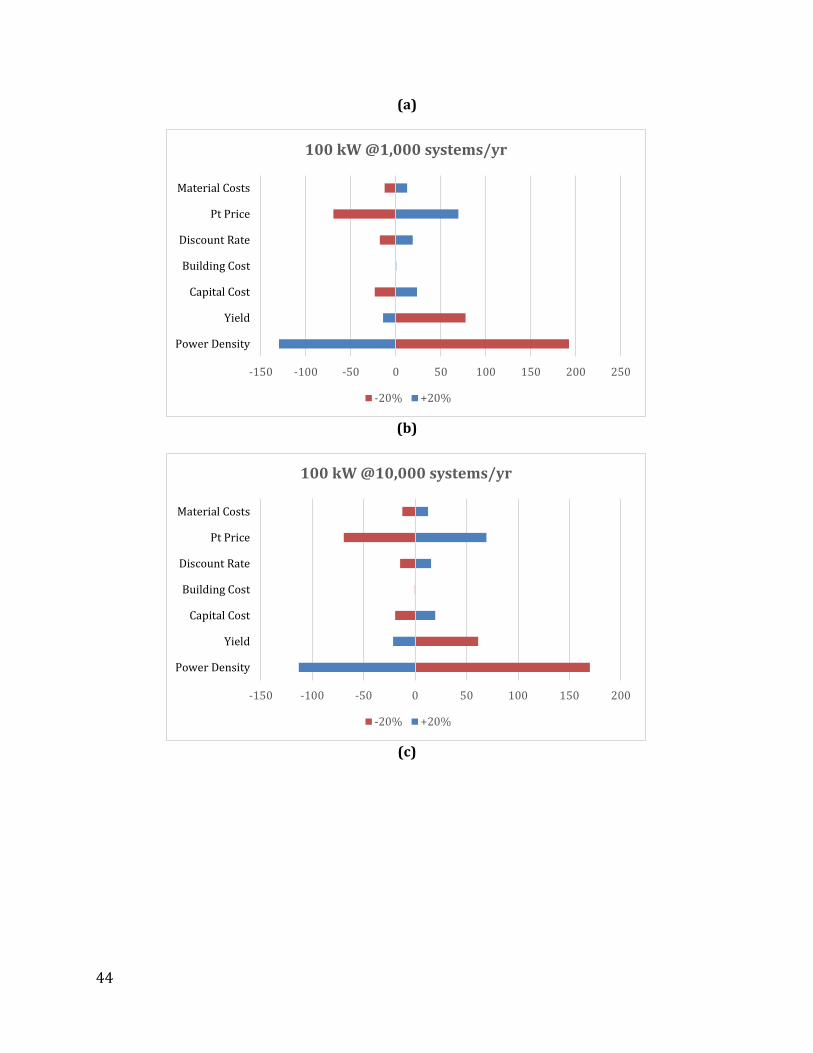
2.6. Sensitivity Analysis Sensitivity analysis was done for 100kWe systems at different production volumes (as shown below in Figure 2.27). The impact of changing several parameters on the stack cost is calculated for a ±20% change in the sensitivity parameter being varied. Power density and process yield tend to be the most sensitive parameters that change the cost of the stack, followed by Pt price and capital cost which also have significant effect on the stack cost at all production volumes. At low volume, overall yield, capital cost and power density are the largest contributing factors, while at higher production volumes the cost is more sensitive to the changes in the process yield and power density. Sensitivity analyses for stack modules are included in Appendix B.

0

4

8

12

16

100 1000 10000 50000

$/kW

system/yr

Stack Assembly Cost ($/kW) 100 kW FC System

Direct Materials

Direct Labor

Process: Capital

Process: Operational

Process: Building

-200 -150 -100 -50 0 50 100 150 200 250

Power Density

Yield

Capital Cost

Building Cost

Discount Rate

Pt Price

Material Costs

100 kW @100 systems/yr

-20% +20%

44

(a)

(b)

(c)

-150 -100 -50 0 50 100 150 200 250

Power Density

Yield

Capital Cost

Building Cost

Discount Rate

Pt Price

Material Costs

100 kW @1,000 systems/yr

-20% +20%

-150 -100 -50 0 50 100 150 200

Power Density

Yield

Capital Cost

Building Cost

Discount Rate

Pt Price

Material Costs

100 kW @10,000 systems/yr

-20% +20%

45

(d)

Figure 2.27. Sensitivity analysis plots for the stack cost. Plots show equivalent area for 100 kWe system expressed in ($/kWe) at different annual production rates: (a) 100 system/year; (b) 1,000 system/year; (c) 10,000 system/year; and (d) 50,000 system/year. (Note: “Material Costs” exclude Pt cost)

-150 -100 -50 0 50 100 150 200

Power Density

Yield

Capital Cost

Building Cost

Discount Rate

Pt Price

Material Costs

100 kW @ 50,000 systems/yr

-20% +20%

46

3. Balance of Plant and Fuel Processor Cost Balance of plant (BOP) component and cost analysis done for HT PEMFC combined heat and power (CHP) systems with reformate fuel. Several system capacities were analyzed (1, 10, 50, 100, and 250kWe) at various annual production volumes (100, 1000, 100,00 and 50,000 systems per year). The BOP analysis is based on the earlier LT PEM report (Wei et al., 2014) with system modifications and simplifications appropriate for the HT PEM technology.

3.1 BOP Costing Approach The general approach is a bottom-up costing analysis based on the system designs described above using existing LT PEM and phosphoric acid fuel cell systems5, industry advisors, and various FC system specification sheets for data sources. There are very few to no actively operating HT PEM CHP systems, so other technologies were consulted and adopted to the HT PEM case. Methods of determining the representative components found in this model range from inspection of existing stationary fuel cell systems, information gathered through surveys of industry partners, discussions and price quotes with vendors, and utilization of components used for common but similar functions in other applications. Thus, the system represented here reflects the authors’ best assessment of existing or planned systems but does not necessarily capture all system components with exact fidelity to existing physical systems, nor does there exist a physical system that is exactly the same as that described here. The BOP is divided into six subsystems or subareas listed below: 1. Fuel Subsystem 2. Air Subsystem 3. Coolant Subsystem and Humidification Subsystems 4. Power Subsystem 5. Controls & Meters Subsystem 6. Miscellaneous Subsystem BOP costing is based on component inventory based on the CHP system diagram, component costs, and earlier work on low temperature PEM systems (Tables 3.1 and 3.2). Non-fuel processor BOP costs assume purchased components while fuel processor costing (Table 3.3) is based on earlier bottom-up cost analysis by Strategic Analysis (James 2012). The HT PEM BOP and FP costs are slightly lower (10-15%) than LT PEM BOP and FP due to system simplifications for HT PEM compared to LT PEM. These include greater CO tolerance of the stack, no air slip to anode, and no stack humidification required. 5 In particular, balance of plant study was done on two CHP systems in the field: (1) the Ballard 1.1MWe ClearGen® system (LT PEM) installed in Torrance, CA and (2) a 5kWe Doosan CHP system (PAFC) installed in Oakland, CA. More details on the Ballard installation can be found in Wei et al. (2014).

47

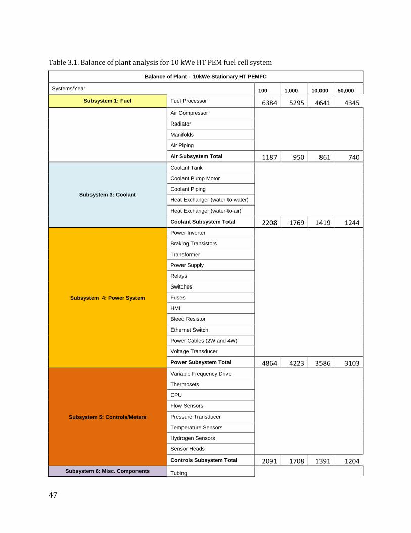
Table 3.1. Balance of plant analysis for 10 kWe HT PEM fuel cell system

Balance of Plant - 10kWe Stationary HT PEMFC

Systems/Year 100 1,000 10,000 50,000

Subsystem 1: Fuel Fuel Processor 6384 5295 4641 4345

Air Compressor

Radiator

Manifolds

Air Piping

Air Subsystem Total 1187 950 861 740

Subsystem 3: Coolant

Coolant Tank

Coolant Pump Motor

Coolant Piping

Heat Exchanger (water-to-water)

Heat Exchanger (water-to-air)

Coolant Subsystem Total 2208 1769 1419 1244

Subsystem 4: Power System

Power Inverter

Braking Transistors

Transformer

Power Supply

Relays

Switches

Fuses

HMI

Bleed Resistor

Ethernet Switch

Power Cables (2W and 4W)

Voltage Transducer

Power Subsystem Total 4864 4223 3586 3103

Subsystem 5: Controls/Meters

Variable Frequency Drive

Thermosets

CPU

Flow Sensors

Pressure Transducer

Temperature Sensors

Hydrogen Sensors

Sensor Heads

Controls Subsystem Total 2091 1708 1391 1204 Subsystem 6: Misc. Components Tubing

48

Wiring

Enclosure Fasteners

Fire Detection Panel

Misc. Components Total 3012 2616 2326 1775

Total BOP Cost $/system 19750 16560 14230 12410 $/kWe 1975 1656 1423 1241

Table 3.2. Balance of plant analysis for 100 kWe HT PEM fuel cell system

Balance of Plant - 100kWe Stationary HT PEMFC

Systems/Year 100 1,000 10,000 50,000

Subsystem 1: Fuel Fuel Processor 23056 20328 18920 18216

Air Compressor

Air Pump Motor

Radiator

Air Piping

Manifolds

Air Subsystem Total 4196 3330 3121 2806

Subsystem 3: Coolant

Coolant Tank

Coolant Pump Motor

Coolant Piping

Heat Exchanger (water-to-water)

Heat Exchanger (water-to-air)

Coolant Subsystem Total 11088 9208 7786 7112

Subsystem 4: Power System

Power Inverter

Braking Transistors

Transformer

Power Supply

Relays

Switches

Fuses

HMI

Bleed Resistor

Ethernet Switch

Power Cables (2W and 4W)

Voltage Transducer

Power Subsystem Total 27166 24455 21353 18262

Subsystem 5: Controls/Meters

Variable Frequency Drive

Thermosets

CPU

49

Flow Sensors

Pressure Transducer

Temperature Sensors

Hydrogen Sensors

Sensor Heads

VPN

Controls Subsystem Total 12215 9935 8086 7173

Subsystem 6: Misc. Components

Tubing

Wiring

Enclosure Fasteners

Fire Detection Panel

Misc. Components Total 7590 6097 4908 4395

Total BOP Cost $/system 85300 73400 64200 58000

$/kWe 853 734 642 580

Table 3.3. summarizes cost of the fuel processor in ($/kWe) based on earlier work by SA.

Table 3.3. Fuel processor costs in $/kWe.

Annual production volume (systems/yr)

FC system size 100 1000 10000 50000 1 kWe 3730 2871 2438 2241 10 kWe 638 530 464 435 50 kWe 258 223 204 195 100 kWe 231 203 189 182 250 kWe 198 179 171 165

50

4. Fuel Cell System Direct Manufacturing Costing Results

4.1. HT PEM Fuel Cell System Costing Results System costing results are shown below for CHP systems with reformate fuel at 10kWe and 100 kWe system sizes. These represent a synthesis of system designs and functional specifications, DFMA costing analysis for FC stack components, and the BOP costing discussion from the preceding chapters. Two sets of plots are shown: (1) overall system costs per kWe as function of production volume (100, 1000, 10000, and 50000 systems per year) as shown in Figure 4.1, and (2) a breakout of the FC stack costs as a percentage of overall costs as shown in Figure 4.2. Additional cost plots can be found in Appendix C. It is important to distinguish direct cost numbers representing direct manufacturing (or purchased parts for BOP) and “customer cost” numbers, which include corporate markups such as profit margin, G&A, sales and marketing, warranty costs, etc. Typical markups are expected to about 40% to 60% for the final “factory gate” price, not including shipping to the customer location. A final cost component is installation costs and other fees, which include site installation costs, permitting fees, and any other fees. (a)

(b)

Figure 4.1. System cost vs annual production volume for (a) 10kWe and (b) 100kWe HT PEM CHP system with reformate fuel.

$0

$500

$1,000

$1,500

$2,000

$2,500

$3,000

$3,500

$4,000

$4,500

$5,000

100 1,000 10,000 50,000

Cost

/kW

(201

3 $)

Production Volume (Systems/year)

Fuel Processor

BOP

Material Scrap ($/kWnet)

Process: Building ($/kWnet)

Process: Operational ($/kWnet)Process: Capital ($/kWnet)

Labor ($/kWnet)

Direct Material ($/kWnet)

Stack

$- $200 $400 $600 $800

$1,000 $1,200 $1,400 $1,600 $1,800 $2,000

100 1,000 10,000 50,000

Cost

/kW

(201

3 $)

Production Volume (Systems/year)

Fuel Processor

BOP

Material Scrap ($/kWnet)

Process: Building ($/kWnet)

Process: Operational ($/kWnet)

Process: Capital ($/kWnet)

Labor ($/kWnet)

Direct Material ($/kWnet)

Stack

51

(a)

(b)

Figure 4.2. Stack cost breakdown for: a) 10kWe; and b) 100kWe fuel cell system

Table 4.1 summarizes fuel cell system cost broken out by stack, BOP and fuel processer.

0%10%20%30%40%50%60%70%80%90%

100%

100 1000 10000 50000Production Volume (Systems/year)

Stack Cost Breakdown (10 kW FC System)

Assembly

Plates

Frame/Sealing

GDE

Membrane

0%10%20%30%40%50%60%70%80%90%

100%

100 1000 10000 50000Production Volume (Systems/year)

Stack Cost Breakdown (100 kW FC System)

Assembly

Plates

Frame/Sealing

GDE

Membrane

52

Table 4.1. HT PEM fuel cell system cost summary (in $/kWe)

Annual production volume (syst./yr)

Stack Cost

FC system size

100 1000 10000 50000

1 kWe 16102 2843 1276 937 10 kWe 2629 1108 771 701 50 kWe 1290 805 688 638

100 kWe 1059 741 649 601 250 kWe 889 705 628 610

FC system size

100 1000 10000 50000

BOP and

Fuel Processor summary

1 kWe 11065 9050 7674 6744 10 kWe 1974 1656 1423 1241 50 kWe 1076 934 818 718

100 kWe 853 734 642 580 250 kWe 730 645 574 511

FC system size

100 1000 10000 50000

Fuel Cell System Cost

1 kWe 27167 11893 8950 7681 10 kWe 4603 2764 2194 1942 50 kWe 2366 1739 1506 1356

100 kWe 1912 1474 1290 1181 250 kWe 1619 1350 1202 1121

Table 4.2. Cost reduction of the HT PEM fuel cell system as a function of the annual production volume

Annual production volume (syst./yr)

Stack Cost

FC system size 100 to 1000

syst./yr

1000 to 10000

syst./yr

10000 to 50000

syst./yr 1 kWe 82% 55% 27%

10 kWe 58% 30% 9% 50 kWe 38% 15% 7%

100 kWe 30% 12% 7% 250 kWe 21% 11% 3%

FC system size 100 to 1000

syst./yr

1000 to 10000

syst./yr

10000 to 50000

syst./yr

BOP and Fuel

Processor summary

1 kWe 18% 15% 12% 10 kWe 16% 14% 13% 50 kWe 13% 12% 12%

100 kWe 14% 13% 10% 250 kWe 12% 11% 11%

53

FC system size 100 to 1000

syst./yr

1000 to 10000

syst./yr

10000 to 50000

syst./yr

Fuel Cell System Cost

1 kWe 56% 25% 14% 10 kWe 40% 21% 11% 50 kWe 27% 13% 10%

100 kWe 23% 12% 8% 250 kWe 17% 11% 7%

Table 4.3. Stack cost as percentage of system costs ($/kWe)

Annual production volume (sys/yr) FC system

size 100 1000 10000 50000

1 kWe 59% 24% 14% 12% 10 kWe 57% 40% 35% 36% 50 kWe 55% 46% 46% 47% 100 kWe 55% 50% 50% 51% 250 kWe 55% 52% 52% 54%

Discussion of System Costs Note that system costs above are direct costs only and do not include any corporate markups or installation costs. For 10kWe CHP systems, costs at low volume (100 systems/year) are about $4600/kWe and about $1950/kWe at high volume (50,000 system/year). For 100kWe CHP systems, costs at low volume (100 systems/year) are about $1900/kWe and about $1200/kWe at high volume (50,000 system/year). Stack costs for both the 10kWe and 100kWe system size are dominated by the GDE, with the GDE constituting about 50-70% of the total stack cost across all production volumes. The plates are the second most costly stack component comprising from 17-23% of total stack cost (Figure 4.2). Overall system costs vs. volume are reduced more for the 10kWe case than the 100kWe case. The 10kWe case is on a steeper portion of the cost-versus-volume curve for stack components with a large reduction in stack costs with increasing volume due to greater tool utilization. The 100kWe case is on a flatter portion of the stack cost curve and thus has lower cost reduction versus volume. In moving from 100 to 1000 systems, the stack cost declination is about two to four times greater than the BOP and Fuel Processor (Table 4.2). This is due to the cost reductions from greater tool utilization and automated processes for the fuel cell stack whereas the BOP components are largely assumed to be purchased commodity products with less cost reduction potential. Stack costs as a percentage of total costs are fairly flat at 50-55% of total system cost for the 100kWe system size, but stack cost is reduced from about 57% of total system cost to about 36% for the 10kWe system at high volume. This is mainly due to the larger relative cost reduction in stack costs for the 10kWe system size.

54

The 1kWe system at low volume has artificially high cost due to the assumption of vertically integrated production and extremely low tool utilization at these low volumes. A more realistic cost estimate would rely on more in-house manual labor rather than automated equipment, more purchased components, and potentially outsourced assembly. Since the focus of the study is higher volume production, the research team did not optimize the low volume 1kWe cost estimates with these considerations. Installed Costs of HT PEM CHP Systems Assuming a 50% corporate markup and 33% additional cost for installation and other fees, the installed cost for a 10kWe and 100kWe CHP system are shown in Figures 4.3 and 4.4, respectively. This work did not explore installation costs in detail but relies on other sources for this installation cost (e.g., EPA 2008). The installed cost for 10kWe and 100kWe systems at 1000 systems per year are estimated to be $5500/kWe and $2950/kWe, respectively, while at 50,000 systems per year, installed system costs are reduced to $3900/kWe and $2400/kWe, respectively.

Figure 4.3. Installed cost as a function of volume for 10kWe CHP system.

0

1000

2000

3000

4000

5000

6000

7000

8000

9000

10000

100 1000 10000 50000

$/kW

Annual Production Volume (Systems/year)

33% Installation and Other Fees50% Corporate MarkupBOP and FPStack

55

Figure 4.4. Installed cost as a function of volume for 100kWe CHP system.

4.2. Comparison between HT PEM and LT PEM Fuel Cell Systems The purpose of this section is to provide a cost comparison to the low temperature PEM system. The low temperature cost data comes from the research team’s previous work (Wei, et al., 2014) on LT PEM fuel cell cost analysis. Figure 4.5 compares the stack cost of LT PEM and HT PEM systems for CHP applications. It is seen that the HT PEM stack cost at low production volumes (10kWe, 100systems/yr) is about $840/kWe (47%) higher than the LT stack cost while at high production volumes (100kWe, 50,000 systems/yr), stack cost is $360/kWe (153%) higher. At all production volumes, the HT GDE/membrane combination is has a higher cost than the LT GDL/catalyst coated membrane combination. Catalyst is deposited on to the GDL in the HT PEM stack versus depositing the catalyst to the membrane for LT PEM stack, and the HT PEM case has higher Pt loading at 0.7mg/cm2 vs 0.5mg/cm2 for the LT case. The plates are also more costly in the HT case due to the use of compression molding and the adoption of a separator layer as described in Chapter 3. In addition, the power density (W/cm2) of the HT PEM stack is lower than the LT stack by about 40%, which in turn necessitates larger cell area or a greater number of cells for the same level of electrical output. The HT PEM cell area in our case is about twice as large compared to the LT PEM cell considered in the earlier LT PEM report. This necessitates result in higher overall material costs and higher overall stack costs for the HT PEM fuel cell case.

0

500

1000

1500

2000

2500

3000

3500

4000

4500

100 1000 10000 50000

$/kW

Annual Production Volume (Systems/year)

33% Installation and Other Fees50% Corporate MarkupBOP and FPStack

56

(a)

(b)

Figure 4.5. Stack cost comparison w/ component breakdown (a) 10kWe (b) 100kWe Figure 4.6 shows the stack cost comparison with a manufacturing cost breakdown and illustrates that the majority of the cost difference between the LT PEM and HT PEM systems is from the differences in material cost. The driving factor behind increased material cost is the increased cell area and stack size. The HT stack also has higher Pt loading at 0.7mg/cm2 vs 0.5mg/cm2 for the LT case.

0

500

1000

1500

2000

2500

3000

LT HT LT HT LT HT LT HT

$/kW

100 1,000 10,000 50,000 Systems/yr

Frame/Sealing

Assembly

Plates

GDL/GDE

Membrane

0

200

400

600

800

1000

1200

LT HT LT HT LT HT LT HT

$/kW

100 1,000 10,000 50,000 Systems/yr

Frame/SealingAssemblyPlatesGDL/GDEMembrane

57

(a)

(b)

Figure 4.6. Stack cost comparison w/ manufacturing breakdown (a) 10kWe (b) 100kWe Figure 4.7 shows a system cost comparison of the LT and HT PEM fuel cell systems. At low production volumes (10kWe, 100 systems/year), the HT system cost is $550/kWe (14%) greater than the LT system. At high production volumes (100kWe, 50,000 systems/yr), the HT system cost is $320/kWe (31%) greater than the LT system. The larger cost differential at high volumes is due to the fact that stack costs make up a larger fraction of overall costs for the HT case than the LT case.

0

500

1000

1500

2000

2500

3000

LT HT 0 LT HT 0 LT HT 0 LT HT

$/kW

100 1,000 10,000 50,000 Systems/yr

Scrap/WasteProcess: BuildingProcess: OperationalProcess: CapitalDirect LaborDirect Materials

0

200

400

600

800

1000

1200

LT HT 0 LT HT 0 LT HT 0 LT HT

$/kW

100 1,000 10,000 50,000 Systems/yr

Scrap/WasteProcess: BuildingProcess: OperationalProcess: CapitalDirect LaborDirect Materials

58

The HT case has 10-15% lower FP and BOP costs due to system simplification from less need for CO clean up, no air slip to anode, and no membrane humidification. This reduction in FP/BOP costs, however, is not sufficient to compensate for higher stack costs. In conclusion, current cost estimates for HT PEM CHP systems are more costly than analogous LT PEM CHP system costs due to three main factors: (1) lower current density and higher cell areal size, (2) more complex plate design and expensive plate process, and (3) higher catalyst loading. Development in HT PEM technology should focus on these areas for further cost reduction as well as developing high yield, automated processes that are assumed above.

(a)

(b)

Figure 4.7. System cost comparison (a) 10kWe (b) 100kWe

0

500

1000

1500

2000

2500

3000

3500

4000

4500

5000

LT HT LT HT LT HT LT HT

$/kW

100 1,000 10,000 50,000 Systems/yr

FP

BOP non FP

Stack

0

500

1000

1500

2000

2500

LT HT LT HT LT HT LT HT

$/kW

100 1,000 10,000 50,000 Systems/yr

FP

BOP non FP

Stack

59

5 Total Cost of Ownership Modeling of CHP Fuel Cell Systems

A total cost of ownership (TCO) model was developed for HT PEMFC CHP systems, which take into account capital costs, fuel costs, operating costs, maintenance costs, end-of-life values, heating fuel savings, and externalities. Annual cost of ownership is critically dependent on the assumed duty cycle of operation of the equipment, resulting in the so- called system utilization6. The most economic duty cycle for any given CHP installation depends on several complex factors, including site variables such as space heating requirements, prevailing utility rates and “standby charges7” and site requirements. Various types of tools and analyses can help in addressing these key TCO considerations. Similar to the LT PEMFC report, in this chapter, we present the key components of the TCO model including life cycle cost modeling (LCC) and results of life cycle impact assessment modeling (LCIA). Total cost of ownership “TCO” modeling is also included as a roll-up summary of the costing models for several commercial building types in six different cities including Phoenix, Arizona, Minneapolis, Minnesota, Chicago, Illinois, New York City, New York, Houston, Texas, and San Diego, California. These cities were chosen to represent several climate zones within the United States.

5.1. Use-phase Model Figure 5.1 below shows the logic used in developing the use-phase model for a 10kWe fuel cell system. This model has four inputs: electricity demand excluding cooling loads, electricity demand solely for space cooling using traditional electrically-driven vapor-compression air conditioners, hot water heating demand, and space heating demand as a function of time, as recorded in daily load curves for three different days per month (weekday, weekend and peak day). These load shapes were collected from an NREL modeling simulation (Deru et al., 2011). The operating mode of this system will follow the total electricity load (sum of ‘non-cooling electricity load’ and ‘electricity for cooling load’). The fuel cell system will cover all of the electrical demand at any time; however, if the total demand exceeds fuel cell capacity (i.e. total electricity loads >10kWe) then the system will cover 10 kWe only and the remaining will be purchased directly from the grid. Similar logic is used for heating demand. Table 5.1 below shows the system cost and operation and maintenance (O&M) cost assumed for HT PEM systems. These installed costs are taken directly from the system cost estimates in the previous chapter for annual volumes assumed to be 100MW per year (e.g., 10,000 x 10kWe systems per year. More details about use-phase model and assumptions can be found in the LT PEMFC report.

6 In this report, system availability is the percentage of hours in the year that the FCS is available for operation. For example, the system may not be available some hours due to scheduled maintenance or unscheduled outages. The system utilization is then defined as the percentage of kWhe produced by the fuel cell system out of the total kWhe of potential output at the nameplate power rating of the system and for available hours of operation. 7 Standby rates are charges levied by utilities when a distributed generation system, such as an on-site CHPsystem, experiences a scheduled or emergency outage, and then must rely on power purchased from the grid. These charges are generally composed of two elements: energy charges, in $/kWh, which reflect the actual energy provided to the CHP system; and demand charges, in $/kW, which attempt to recover the costs to the utility of providing capacity to meet the peak demand of the facility using the CHP system. Source: ACEEE, http://www.aceee.org/topics/standby-rates, accessed 5/29/14.

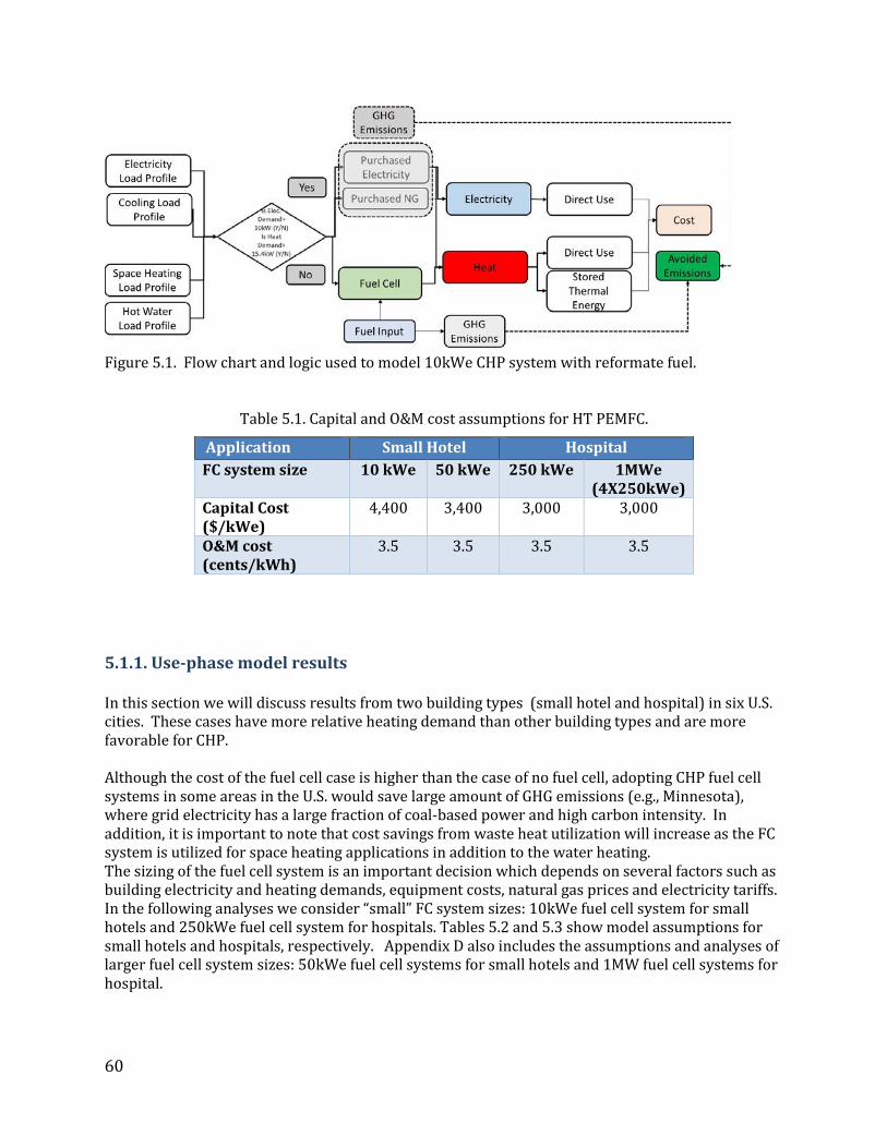
60

Figure 5.1. Flow chart and logic used to model 10kWe CHP system with reformate fuel.

Table 5.1. Capital and O&M cost assumptions for HT PEMFC.

Application Small Hotel Hospital FC system size 10 kWe 50 kWe 250 kWe 1MWe

(4X250kWe) Capital Cost ($/kWe)

4,400 3,400 3,000 3,000

O&M cost (cents/kWh)

3.5 3.5 3.5 3.5

5.1.1. Use-phase model results

In this section we will discuss results from two building types (small hotel and hospital) in six U.S. cities. These cases have more relative heating demand than other building types and are more favorable for CHP. Although the cost of the fuel cell case is higher than the case of no fuel cell, adopting CHP fuel cell systems in some areas in the U.S. would save large amount of GHG emissions (e.g., Minnesota), where grid electricity has a large fraction of coal-based power and high carbon intensity. In addition, it is important to note that cost savings from waste heat utilization will increase as the FC system is utilized for space heating applications in addition to the water heating. The sizing of the fuel cell system is an important decision which depends on several factors such as building electricity and heating demands, equipment costs, natural gas prices and electricity tariffs. In the following analyses we consider “small” FC system sizes: 10kWe fuel cell system for small hotels and 250kWe fuel cell system for hospitals. Tables 5.2 and 5.3 show model assumptions for small hotels and hospitals, respectively. Appendix D also includes the assumptions and analyses of larger fuel cell system sizes: 50kWe fuel cell systems for small hotels and 1MW fuel cell systems for hospital.

61

Model results in Table 5.4 show the results of utilizing a fuel cell system to augment purchased electricity and purchased fuel for conventional heating compared to the case of no fuel cell and just relying on purchased electricity and conventional heating. For a small hotel, the annuitized cost of supplying all building electricity and heating increases with the use of fuel cells by an amount between about 3% in Minneapolis, MN to about 27% in Houston, TX when the FC system supplies both space heating and water heating. For the hospital (Table 5.5), the annuitized cost with fuel cells increases in the range of 10% for fuel cell system installed in Chicago compared to a 28.2% cost increase for a fuel cell system installed in New York, NY. Here, without any additional credits, a potential niche market was located for small hotels located in Minneapolis, MN. In general, as the in-use heat utilization increases, the economics and positive environmental impacts of CHP fuel cell systems also rise (Colella et al., 2010). For the small hotel, as shown in Table 5.4, the overall heat recovery utilization of a system installed is 54% if the FC system utilizes for both space and water heating for a system installed in Houston, TX. The heat utilization is much higher for a system installed in other cities like Minneapolis which reaches 100% when the FC system both space and water heating demands. For the hospital, as shown in Table 5.5, the overall heat recovery efficiency of a system installed is relatively high; approximately 75%, for a system installed in Houston, but can reach 100% for a system installed in New York City.8 Table. 5.2. Assumptions for cost and environmental impact model for small hotel case.

Parameter Phoenix, AZ

Minneapolis, MN

Chicago, IL

NYC, NY Houston, TX

Unit

Building Type Small Hotel FC system size 10 kWe Capital costs of FC including installation cost

4,400

$/kWe

Electricity price Variable by time

Variable by time

Variable by time

Variable by time

Variable by time

$/kWh

Demand Charge 4.05 3.30 5.69 17.95 12.39 15.13 (June-Sep)

$ * Peak kWh

NG cost 0.0357 0.0258 0.0292 0.0332 0.0263 $/kWh Scheduled maintenance cost ‡

500 500 500 500 500 $/yr

O&M cost 0.035 0.035 0.035 0.035 0.035 $/kWh Days per year 365 365 365 365 365 day FC system availability‡‡

96% 96% 96% 96% 96%

Lifetime of system 15 15 15 15 15 yr Interest rate 5% 5% 5% 5% 5%

‡ From CETEEM model (Lipman et al., 2004). ‡‡ In this analysis the CHP system was assumed to have a 96% availability factor and three outages during the year. One outage is assumed to be a planned maintenance outage and two are assumed to be unplanned forced outages.

8 Note the “Annual generated heat by FC” in Tables 5.4 and 5.5 reflect the thermal efficiency in Table 1.2 so that a “100% heat utilization” means that the full thermal efficiency of the CHP system has been realized.

62

Table. 5.3. Life cycle cost analysis assumptions for hospital case (250kWe FC system).

Parameter Phoenix, AZ

Minneapolis, MN

Chicago, IL

NYC, NY Houston, TX

San Diego, CA

Unit

Building Type Hospital FC system size 250 kWe Capital costs of FC including installation cost

3,000

$/kWe

Electricity price Variable by time

Variable by time

Variable by time

Variable by time

Variable by time

$/kWh

Demand Charge 4.05 8.98 12.86 (June-

Sep)

5.86 17.95 12.39 15.13 (June-Sep)

19.96 $ * Peak kWh

NG cost 0.0357 0.0258 0.0292 0.0332 0.0263 0.0277 $/kWh Scheduled maintenance cost ‡

3,000 3,000 3,000 3,000 3,000 $/yr

O&M cost 0.035 0.035 0.035 0.035 0.035 $/kWh FC system availability‡‡

96% 96% 96% 96% 96%

Lifetime of system 15 15 15 15 15 yr Interest rate 5% 5% 5% 5% 5% From CETEEM model (Lipman et al., 2004). ‡‡ In this analysis the CHP system was assumed to have a 96% availability factor and three outages during the year. One outage is assumed to be a planned maintenance outage and two are assumed to be unplanned forced outages.

63

Table 5.4. Output results from use-phase model for small hotel (10 kWe FC system)

† CO2 emissions only. * O&M cost = $0.035/kWh WH: water heating; and SH: space heating

OutputNo Fuel

CellFuel Cell

No Fuel Cell

Fuel CellNo Fuel

CellFuel Cell

No Fuel Cell

Fuel CellNo Fuel

CellFuel Cell

FC System Utilization 100.0% 100.0% 100.0% 100.0% 100.0%FC Heat Utilization WH+SH 66.0% 100.0% 100.0% 100.0% 54.0%Total Electricity Demand (kWh/yr) Total Space Heating Demand (kWh/yr) Total Water Heating Demand (kWh/yr) Annual Generated Power by FC (kWh) 84,096 84,096 84,096 84,096 84,096Annual Generated Heat by FC (kWh) 145,541 145,541 145,541 145,541 145,541

Capital Cost 0 4,239 0 4,239 0 4,239 0 4,239 0 4,239O&M Cost 0 2,943 0 2,943 0 2,943 0 2,943 0 2,943Scheduled Maintenance 0 500 0 500 0 500 0 500 0 500Fuel Cost-FC Only 0 9,959 0 7,199 0 8,165 0 9,260 0 7,347Residual Fuel 3,574 319 7,779 4,238 7,449 3,489 8,352 3,875 2,185 84Electrcity Cost 47,305 40,333 45,374 35,998 32,104 25,495 8,798 6,713 15,427 12,712Demand Charge 5,445 5,093 3,422 3,125 6,021 5,508 16,959 15,344 15,490 14,321Fixed Monthly Charge 150 150 131 131 348 348 1,241 1,241 295 295Cost ($/yr) FC supplies both space heating and Hot water 56,473 63,536 56,706 58,373 45,922 50,688 35,350 44,115 33,397 42,442GHG (ton CO2/yr) FC supplies hot water only 298.483 289.283 404.7 351.995 338.787 289.787 147.998 129.198 277.3 268.8

Capital Cost 0 4,239 0 4,239 0 4,239 0 4,239 0 4,239O&M Cost 0 2,943 0 2,943 0 2,943 0 2,943 0 2,943Scheduled Maintenance 0 500 0 500 0 500 0 500 0 500Fuel Cost-FC Only 0 9,959 0 7,199 0 8,165 0 9,260 0 7,347Residual Fuel 3,574 929 7,779 5,104 7,449 4,517 8,352 5,063 2,185 84Electrcity Cost 47,305 40,333 45,374 35,998 32,104 25,495 8,798 6,713 15,427 12,712Demand Charge 5,445 5,093 3,422 3,125 6,021 5,508 16,959 15,344 15,490 14,321Fixed Monthly Charge 150 150 131 131 348 348 1,241 1,241 295 295Cost ($/yr) FC supplies both space heating and Hot water 56,473 64,147 56,706 59,239 45,922 51,716 35,350 45,303 33,397 42,442GHG (ton CO2/yr) FC supplies both space heating and Hot water 298.483 294.683 404.7 356.595 338.787 297.487 147.998 133.198 277.3 268.8

Minneapolis, Chicago, IL NYC, NY Houston, TXPhoenix, AZ

369,661

135,869

116,075

497,656

0

83,071

419,590

174,743

127,112

424,147

135,869

118,971

576,668

23,307

76,954

FC supplies hot water only

FC supplies both space and water heating

64

Table 5.5. Output results from use-phase model for hospital (250kWe FC system).

† CO2 emissions only. * O&M cost = $0.035/kWh WH: water heating; and SH: space heating

5.2. Life Cycle Impact Assessment (LCIA) Modeling Similar to the approach we used for LT PEMFC, we developed an LCIA model to quantify the environmental and human health damages caused by fuel cell systems in commercial buildings. These fuel cells displace grid-based electricity and some fraction of heating demand fuel, as specified by the user of the model. We calculate an average electricity intensity that is displaced by the FCS and use commercial building surveys to estimate the mix of heating fuel types by region that is displaced by the FCS. Externalities to be valued include morbidity, mortality, impaired

OutputNo Fuel

CellFuel Cell

No Fuel Cell

Fuel CellNo Fuel

CellFuel Cell

No Fuel Cell

Fuel CellNo Fuel

CellFuel Cell

No Fuel Cell

Fuel Cell

FC Power Utilization 100.0% 100.0% 100.0% 100.0% 100.0% 93.0%FC Heat Utilization WH+SH 71.9% 98.2% 93.6% 100.0% 75.3% 15.4%Total Electricity Demand (MWh/yr) 7,331Total Space Heating Demand (MWh/yr) Total Water Heating Demand (MWh/yr) Annual Generated Power by FC (MWh) 2,102 2,102 2,102 2,102 2,102 1,965Annual Generated Heat by FC (MWh) 3,550 3,550 3,550 3,550 3,550 3,527

Capital Cost 0 72,257 0 72,257 0 72,257 0 72,257 0 72,257 0 72,257O&M Cost 0 73,584 0 73,584 0 73,584 0 73,584 0 73,584 0 68,764Scheduled Maintenance 0 3,000 0 3,000 0 3,000 0 3,000 0 3,000 0 3,000Fuel Cost-FC Only 0 253,211 0 183,037 0 207,612 0 235,455 0 186,801 0 182,188Residual Fuel 100,839 4,414 99,542 15,181 107,626 10,494 142,926 26,219 77,908 4,903 16,759 0Electrcity Cost 628,966 478,999 449,323 315,087 593,645 428,409 181,449 129,327 295,508 227,618 186,343 10,951Demand Charge 63,848 52,624 147,992 119,111 87,490 71,101 260,526 210,542 215,513 178,937 67,485 23,511Fixed Monthly Charge 6,367 6,367 341 341 516 516 1,241 1,241 295 295 2,794 2,794Cost ($/yr) FC supplies both space heating and Hot water 800,020 944,456 697,198 781,596 789,276 866,973 586,142 751,625 589,224 747,395 273,381 363,465GHG (ton CO2/yr) FC supplies hot water only 4,956 5,225 6,815 5,855 6,084 4,762 2,892 2,504 5,560 5,232 1,162 972

Capital Cost 0 72,257 0 72,257 0 72,257 0 72,257 0 72,257 0 72,257O&M Cost 0 73,584 0 73,584 0 73,584 0 73,584 0 73,584 0 68,764Scheduled Maintenance 0 3,000 0 3,000 0 3,000 0 3,000 0 3,000 0 3,000Fuel Cost-FC Only 0 253,211 0 183,037 0 207,612 0 235,455 0 186,801 0 182,188Residual Fuel 100,839 95,863 99,542 93,617 107,626 101,332 142,926 135,980 77,908 73,944 16,759 14,665Electrcity Cost 628,966 478,999 449,323 315,087 593,645 428,409 181,449 129,327 295,508 227,618 186,343 10,951Demand Charge 63,848 52,624 147,992 119,111 87,490 71,101 260,526 210,542 215,513 178,937 67,485 23,511Fixed Monthly Charge 6,367 6,367 341 341 516 516 1,241 1,241 295 295 2,794 2,794Cost ($/yr) FC supplies hot water only 800,020 1,035,905 697,198 860,033 789,276 957,811 586,142 861,385 589,224 816,437 273,381 378,129GHG (ton CO2/yr) FC supplies hot water only 4,956 5,273 6,815 6,393 6,084 5,846 2,892 3,190 5,560 5,791 1,162 1,470

FC supplies hot water only

FC supplies both space and water heating

9,140

140 76151230

3,6332,689

7,852

3,682

215 210

2,1669,533

29,622 529

7,624

4,311

San Diego, CAHouston, TXNYC, NYChicago, ILMinneapolis, MN

Phoenix, AZ

65

visibility, recreational disruptions, material damages, agricultural and timber damages, and global warming. Details for computing average electricity intensity and the mix of heating fuel types by region are described in LT PEM report (Wei et al., 2014). Direct emission factors reported in recent literature on fuel cells allowed us to determine reasonable estimates for CO2, CH4, N2O, CO, NOX, SOX, PM10 and VOC (Table 5.6). All values are derived for HT PEM fuel cell based on the values given by Colella (2012).

Table 5.6. HT PEM Fuel cell emission factors in grams per kWh

Pollutant g/kWhe CO2 618 NOx 0.008 SOx Negligible

PM10 Negligible VOC Negligible CH4 0.580 CO 0.019

N2O 0.068 Tables 5.7 and 5.8 summarize LCIA results for small hotel case using 10kWe fuel cell system in which waste heat is utilized for water heating only (Table 5.7) and both space and water heating (Table 5.8). Similarly Tables 5.9 and 5.10 summarizes LCIA results for 250kWe fuel cell system used in the hospital case. Table 5.9 summarizes LCIA results when waste heat is used for water heating only, while Table 5.10 summarizes LCIA results when fuel cell system is used for both space and water heating. The calculation of these emissions uses the same modeling approach described in Wei et al. (2014) and a detailed description can be found in that reference. Table 5.7. LCIA results for 10kWe fuel cell system used in the small hotel. Waste heat is utilized for water heating application only.

Output Phoenix Minneapolis ChicagoNew York

City Houston

Annual Generated Power by FC (kWh) 84,096 84,096 84,096 84,096 84,096

Annual Generated Heat by FC (kWh) 145,541 145,541 145,541 145,541 145,541

Avoided GHG [tCO2e/y] 3.8 48.1 41.3 14.8 8.5

Avoided NOx [tNOx/y] 0.042 0.129 0.117 0.049 0.041

Avoided SOx [tSOx/y] 0.033 0.235 0.371 0.075 0.040

Avoided PM10 [t/y] 0.0015 0.0012 0.0014 0.0015 0.00071

Avoided PM2.5 [t/y] 0.000 0.00022 0.00025 0.00039 0.00000

GHG credit at $44/ton CO2 ($/kWhe) 0.002 0.025 0.022 0.008 0.004

Health, Environmental Savings ($/kWhe) 0.003 0.024 0.035 0.016 0.003

66

Table 5.8. LCIA results for 10kWe fuel cell system used in the small hotel. Waste heat is utilized for both space and water heating.

Table 5.9. LCIA results for 250kWe fuel cell system used in the hospital. Waste heat is utilized for water heating application only.

Output Phoenix Minneapolis Chicago New York City

Houston

Annual Generated Power by FC (kWh) 84,096 84,096 84,096 84,096 84,096

Annual Generated Heat by FC (kWh) 145,541 145,541 145,541 145,541 145,541

Avoided GHG [tCO2e/y] 9.2 52.7 49.0 18.8 8.5

Avoided NOx [tNOx/y] 0.047 0.134 0.126 0.052 0.041

Avoided SOx [tSOx/y] 0.038 0.243 0.392 0.083 0.040

Avoided PM10 [t/y] 0.0019 0.0013 0.0017 0.0017 0.00071

Avoided PM2.5 [t/y] 0.00059 0.00026 0.00030 0.00049 0.0000

GHG credit at $44/ton CO2 ($/kWhe) 0.0048 0.028 0.026 0.010 0.0045

Health, Environmental Savings ($/kWhe) 0.0037 0.025 0.037 0.018 0.0026

Output Phoenix Minneapolis ChicagoNew York

City Houston San Diego

Annual Generated Power by FC (MWh) 2,102 2,102 2,102 2,102 2,102 1964.7

Annual Generated Heat by FC (MWh) 3,550 3,550 3,550 3,550 3,550 3,527

Avoided GHG [tCO2e/y] -317 422 238 -298 -231 -308

Avoided NOx [tNOx/y] 0.70 2.32 2.05 0.71 0.70 0.64

Avoided SOx [tSOx/y] 0.39 4.46 7.10 1.20 0.84 0.36

Avoided PM10 [t/y] 0.0022 0.0033 0.0020 0.0033 0.0021 0.00063

Avoided PM2.5 [t/y] 0.00023 0.0006 0.00010 0.00088 0.00011 0.00006

GHG credit at $44/ton CO2 ($/kWhe) -0.0066 0.0088 0.0050 -0.0062 -0.0048 -0.0069

Health, Environmental Savings ($/kWhe) 0.0009 0.0161 0.0256 0.0051 0.0017 0.0015

67

Table 5.10. LCIA results for 250kWe fuel cell system used in the hospital. Waste heat is utilized for both space and water heating.

5.3. Total Cost of Ownership Modeling Results Figure 5.2 outlines the approach for comparing fuel cell total cost of ownership with grid based electricity and conventional heating. A fuel cell CHP system will typically increase the cost of electricity but provide some saving by offsetting heating energy requirements. The cost of fuel cell electricity in this case is taken to be the “levelized cost of electricity” or the levelized cost in $/kWh for the fuel cell system taking into account capital costs, operations and maintenance (O&M), fuel, and capital replacement costs (inverter, stack replacement, etc.) only. In this work we credit all saving from heating fuel savings, electricity demand charge savings, carbon credits from net system savings of CO2eq, and net avoided environmental and health externality damages to the fuel cell system cost of electricity and call this quantity “cost of electricity with total cost of ownership savings.” This allows comparison of fuel cell COE with TCO credits or “total cost of electricity” to the reference grid electricity cost ($/kWh).

Output Phoenix Minneapolis ChicagoNew York

City Houston San Diego

Annual Generated Power by FC (MWh) 2,102 2,102 2,102 2,102 2,102 1964.7

Annual Generated Heat by FC (MWh) 3,550 3,550 3,550 3,550 3,550 3,527

Avoided GHG [tCO2e/y] 269 960 1322 388 328 -190

Avoided NOx [tNOx/y] 1.19 2.79 3.25 1.28 1.17 0.73

Avoided SOx [tSOx/y] 0.55 4.77 10.04 1.90 0.92 0.40

Avoided PM10 [t/y] 0.0445 0.0505 0.0328 0.0558 0.0407 0.00502

Avoided PM2.5 [t/y] 0.00469 0.0094 0.00170 0.01491 0.00210 0.00050

GHG credit at $44/ton CO2 ($/kWhe) 0.0056 0.0201 0.028 0.008 0.0069 -0.0043

Health, Environmental Savings ($/kWhe) 0.0025 0.0223 0.037 0.021 0.0039 0.0020

68

Figure 5.2. Cost of energy service for FC CHP and conventional electricity and heating systems. A fuel cell CHP system will typically increase the levelized cost of electricity (upper left two bars). But if waste heat is utilized, the cost of heating is reduced (upper right two bars). In this treatment, all non-electricity credits (heating, carbon, etc) are applied to a “total cost of electricity” (lower left two bars).

Tables 5.11 and 5.12 summarize TCO results for 10 kWe and 250kWe CHP fuel cell system used in small hotel and hospital, respectively. Results for a 10 kWe fuel cell system used in small hotel in Chicago is shown in Figure 5.4 which shows clearly that fuel cell system can act as a viable economic CHP solution when including a total cost framework and under the assumptions of this study.

Chicago has relatively high carbon intensity electricity due to a significant fraction of coal- powered electricity, and by extension other cities in the Midwest such as Minneapolis are highlighted as a region that is relatively favorable for FC CHP applications in certain commercial building types. For example, for a small hotel with a 10 kWe FCS, space and water heatings can offset 25% of the levelized cost of electricity (Figure 5.3) in Chicago. GHG credits provide 14% savings at $44 per ton of CO2-eq, and health and environmental savings provide 20% savings. Total savings from heating and externalities is almost 60% for the case of CHP with offset water heating and space heating.

69

Table 5.11. TCO results for 10kWe FC system used in small hotel with the FC system providing both water heating and space heating.

No FCS Fuel Cell No FCS Fuel Cell No FCS Fuel Cell No FCS Fuel Cell No FCS Fuel Cell

FC System Utilization 100% 100% 100% 100% 100%

Total Electricity Demand (kWh/yr) 576,668 576,668 419,590 419,590 424,147 424,147 369,661 369,661 497,656 497,656

Total Space Heating Demand (kWh/yr) Total Water Heating Demand (kWh/yr) Annual Generated Power by FC (kWh) 84,096 84,096

84,096 84,096 84,096

FC fraction of Electricity Demand 15% 20% 20% 23% 17%Annual Generated Heat by FC (kWh) 145,541 145,541 145,541 145,541 145,541Capital Cost ($/yr) 4,239 4,239 4,239 4,239 4,239O&M Cost ($/yr) 2,943 2,943 2,943 2,943 2,943Scheduled Maintenance ($/yr) 500 500 500 500 500Fuel Cost for Fuel Cell ($/yr) 9,959 7,199 8,165 9,260 7,347Fuel Cost for Conv. Heating ($/yr) 3574 319 7780 4,238 7450 3,489 8351 3,875 2185 84Purchased Electricity Energy Cost ($/yr) 47305 40333 45374 35998 32104 25495 8798 6713 15427 12712Demand Charge ($/yr) 5445 5093 3422 3125 6021 5508 16959 15344 15490 14321Fixed Charge, Electricity ($/yr) 150 150 131 131 348 348 1241 1241 295 295Total Electrictiy Cost ($/yr) 52899 63217 48927 54135 38473 47198 26998 40239 31213 42357Total Cost of Electricity ($/kWh) 0.092 0.110 0.117 0.129 0.091 0.111 0.073 0.109 0.063 0.085

Purchased Electricity Cost ($/kWh)0.092 0.093 0.117 0.117 0.091 0.092 0.073 0.082 0.063 0.066

LCOE of FC power ($/kWh) 0.210 0.177 0.188 0.201 0.179Fuel savings from conventional heating ($/yr)

3255 3542 3961 4476 2101

Fuel savings per kWh ($/kWh) 0.039 0.042 0.047 0.053 0.025LCOE of FC power with fuel savings ($/kWh)

0.171 0.135 0.141 0.148 0.154

GHG credit at $44/ton CO2

($/kWh)0.0048 0.0276 0.0256 0.0098 0.0045

Health, Environmental Savings ($/kWh)

0.0037 0.0251 0.0373 0.0098 0.0026

LCOE with TCO Savings for Fuel Cell Power ($/kWh)

0.163 0.082 0.078 0.129 0.147

LCOE with TCO Savings for FC and Purchased Power, ($/kWh) 0.103 0.110 0.089 0.092 0.080

OutputPhoenix, AZ Minneapolis, MN Chicago, IL NYC, NY Houston, TX

23,307 174,743 135,869 135,869 0

76,954 127,112 118,971 116,075 83,071

70

Table 5.12. TCO results for 250kWe FC system used in hospital with the FC system providing both water heating and space heating.

No FCS Fuel Cell No FCS Fuel Cell No FCS Fuel Cell No FCS Fuel Cell No FCS Fuel Cell No FCS Fuel Cell

FC System Utilization 100.0% 100.0% 100.0% 100.0% 100.0% 0.94

Total Electricity Demand (MWh/yr) 9,140 9,140 7,331 7,331 7,852 7,852 7,624 7,624 9,533 9,533 2166.4 2166.4

Total Space Heating Demand (MWh/yr) Total Water Heating Demand (MWh/yr) Annual Generated Power by FC (MWh)

2,102 2,102 2,102 2,102 2,102 1965

FC fraction of Electricity Demand 23% 29% 27% 28% 22% 91%Annual Generated Heat by FC (MWh)

3,550 3,550 3,550 3,550 3,550 3,550

Capital Cost ($/yr) 72,257 72,257 72,257 72,257 72,257 72,257O&M Cost ($/yr) 73,584 73,584 73,584 73,584 73,584 68,764Scheduled Maintenance ($/yr) 3,000 3,000 3,000 3,000 3,000 3,000Fuel Cost for Fuel Cell ($/yr) 253,211 183,037 207,612 235,455 186,801 182,188Fuel Cost for Conv. Heating ($/yr) 100839 4,414 99542 15,181 107626 10,494 142926 26,219 77908 4,903 16759 0Purchased Electricity Energy Cost ($/yr)

628966 478,999 449323 315,087 593645 428,409 181449 129,327 295508 227,618 186343 10,951

Demand Charge ($/yr) 63848 52624 147992 119111 87490 71101 260526 210542 215513 178937 67485 23511Fixed Charge, Electricity ($/yr) 6367 6367 341 341 516 516 1241 1241 295 295 2794 2794Total Electricity Cost ($/yr) 699181 940041 597655 766416 681651 856479 443216 725406 511316 742492 256622 363466Total Cost of Electricity ($/kWh) 0.076 0.103 0.082 0.105 0.087 0.109 0.058 0.095 0.054 0.078 0.118 0.168

Purchased Electricity Cost ($/kWh)0.076 0.076 0.082 0.083 0.087 0.087 0.058 0.062 0.054 0.055 0.118 0.185

LCOE of FC power ($/kWh) 0.191 0.158 0.170 0.183 0.160 0.166Fuel savings from conventional heating ($/yr)

96425 84361 97132 116707 73005 16759

Fuel savings per kWh ($/kWh) 0.0459 0.0401 0.0462 0.0555 0.0347 0.0085LCOE of FC power with fuel savings ($/kWh)

0.145 0.118 0.123 0.127 0.125 0.158

GHG credit at $44/ton CO2

($/kWh)0.0056 0.0201 0.0277 0.0081 0.0069 -0.0043

Health, Environmental Savings ($/kWh)

0.0025 0.0223 0.0369 0.0205 0.0040 0.0020

LCOE with TCO Savings for Fuel Cell Power ($/kWh)

0.137 0.075 0.059 0.099 0.114 0.160

LCOE with TCO Savings for FC and Purchased Power, ($/kWh) 0.090 0.081 0.079 0.072 0.068 0.162

OutputPhoenix, AZ Minneapolis, MN Chicago, IL NYC, NY Houston, TX San Diego, CA

75.5

2,689 3,633 3,682 4,311 2812 528.8

140 230 215 210 151

71

Figure 5.3. Levelized and total cost of electricity with TCO credits for a 10kWe small hotel in Chicago, IL for a FC system assumed to provide space heating and water heating.

72

6. Conclusions Although high temperature PEM fuel cell systems still have significant reliability issues to overcome, they offer the advantages of reduced sensitivity to CO poisoning in the input fuel stream, lower cost membrane, and balance of plant simplification. The manufacturing costs presented here represent the authors’ best estimates for longer-lifetime HT PEM technology With the assumptions made in this study, HT PEM systems are higher cost than LT PEM systems, compared to the authors’ recent report on LT PEM CHP systems (Wei et al., 2014). HT PEM CHP direct system costs are about 15% higher at low annual production volumes (100 x 10kWe systems per year) to 30% higher at high volumes (50,000 x 100kWe systems per year). Current cost estimates for HT PEM CHP systems are more costly than LT PEM CHP systems costs due to three main factors: (1) lower current density and higher cell areal size; (2) more complex plate design and expensive plate process; and (3) higher catalyst loading. Bottom up DFMA costing analysis for fuel cell stack components in this work shows that, for stationary applications, HT PEM fuel cell stacks alone can approach a direct manufacturing cost of $600 per kWe of net electrical power at high production volumes (e.g. 100kWe CHP systems at 50,000 systems per year). Overall system costs including corporate markups and installation costs are about $2400/kWe ($2200) for 100kWe (250kWe) CHP systems and about $3900/kWe for 10kWe systems, all at 50,000 systems per year. All fuel cell stack components (membrane, GDE, framed MEA, plates and stack assembly are assumed to be manufactured in-house with high throughput processes and high yield (80%) assumed for all modules. Nearly fully automated roll-to-roll processing is modeled for the critical catalyst coated gas diffusion electrode. While it was not in the scope of this work to do a detailed yield feasibility analysis, well established methodologies exist for improving yield using similar process modules in other industries, and learning-by-doing and improvements in yield inspection, detection, and process control are implicitly assumed. For the fuel cell stack, direct materials costs dominate at high volume as expected and constitute about 80% of stack manufacturing cost for 100kWe CHP systems at a production level of 50,000 systems per year. For the same system size, the GDE is estimated to make up about 65% of the overall stack cost, with the bipolar plates at 20-25% of the total stack cost depending on stack production volume. At low volumes, the stack cost is sharply reduced in moving from a production volume of 100 to 1000 systems per year because tool and equipment utilization increases rapidly. At 100-250kWe system sizes, the stack cost is estimated to fall at a rate between 20-30% in moving from 100 to 1000 systems per year driven by reduced capital costs and lower direct material costs. For overall fuel cell system costs, the stack cost makes up about 50-55% of total costs for 100 kWe systems across the range of production volumes. The cost of electricity with total cost of ownership credits for a fuel cell CHP system has been demonstrated for buildings in six U.S. cities. This approach incorporates the impacts of offset heating demand by the FCS, carbon credits, and environmental and health externalities into a total levelized cost of electricity ($/kWh). This LCOE with total cost of ownership credits can then be compared with the baseline cost of grid electricity. This analysis combines a fuel cell system use-phase model with a life-cycle integrated assessment model of environmental and health externalities. Total cost of electricity will be dependent on the carbon intensity of electricity and heating fuel that a FC system is displacing, and thus highly geography dependent.

73

For the subset of buildings (hotels, hospitals, and office buildings) demand charges, carbon credits, offset water and space heating, and externalities can reduce the total cost of electricity by up to 65% in Chicago but by a much smaller amount in San Diego, which has a lower relative carbon intensity of grid electricity. Health and environmental externalities can provide large savings if electricity or heating with a high environmental impact are being displaced. Overall, this type of total cost of ownership analysis quantification is important to identifying key opportunities for direct cost reduction, to value fully the costs and benefits of fuel cell systems in stationary applications, and to provide a more comprehensive context for future potential policies

74

References ACI Technologies, Inc. “Manufacturing Fuel Cell Manhattan Project.” U.S. Government Contract No. N00014-08-D-0758, November 2011.

Baird, Donald, Jianhua Huang, and James McGrath. "Highly conductive thermoplastic composites for rapid production of fuel cell bipolar plates." Baratto F., Diwekar U.M. “Life cycle assessment of fuel cell-based APUs”. Journal of Power Sources 139 (2005): 188–196. Bhamidipati K.L., Didari, S. Harris, T.A.L. Slot die coating of polybenzimiazole based membranes at the air engulfment limit. Journal of Power Sources 239 (2013) 382-392 Breault, Richard D. "Fuel cell electrolyte reservoir layer and method for making." U.S. Patent No. 4,185,145. 22 Jan. 1980. Breault, Richard D., Warren L. Luoma, and Ronald G. Martin. "Electrochemical cell assembly." U.S. Patent No. 4,929,517. 29 May 1990. Brooks, K. “Fuel Cell Combined Heat and Power Commercial Demonstration.” Pacific Northwest National Laboratory. Prepared for U.S. Department of Energy- Energy Efficiency and Renewable Energy- Office of Fuel Cell Technology May 2014.

Brooks, K. Pilli, S. Makhmalbaf, A. Srivastava, V. Anderson, D. Upton, J. Amaya, J. Business Case for a 5 kW Combined Heat and Power Fuel Cell System. Pacific Northwest National Laboratory. Prepared for U.S. Department of Energy Energy Efficiency and Renewable Energy- Office of Fuel Cell Technology May 2013.

(Coatema) T. Kolbusch, A. Glüsen, J. Mergel. Manufacturing Processes for Gas-Diffusion-Electrodes for Polymer Electrolyte Fuel Cells. 2009 Fuel Cell Seminar & Exposition, Palm Springs, CA, USA November 16-19, 2009.Donald, B. Huang, J. McGrath, J. "Highly conductive thermoplastic composites for rapid production of fuel cell bipolar plates." ELAT 1400 GDE. http://nuvant.com/products/electrode-materials/gas-diffusion-layer/

Cunningham, Brent D., and Donald G. Baird. "Development of bipolar plates for fuel cells from graphite filled wet-lay material and a compatible thermoplastic laminate skin layer." Journal of power sources 168.2 (2007): 418-425. Cunningham, Brent D., Jianhua Huang, and Donald G. Baird. "Development of bipolar plates for fuel cells from graphite filled wet-lay material and a thermoplastic laminate skin layer." Journal of power sources 165.2 (2007): 764-773. Dettling, Charles J., and Peter L. Terry. "Integral gas seal for fuel cell gas distribution assemblies and method of fabrication." U.S. Patent No. 4,505,992. 19 Mar. 1985. EPA 2008, Technology Characterization: Fuel Cells. Prepared for Environmental Protection Agency Combined Heat and Power Partnership Program, Washington, DC by Energy and Environmental Analysis, Inc., an ICF Company, 1655 N. Fort Myer Dr. Suite 600 Arlington, Virginia 22209, December 2008.

75

Haberl, J.S., (1994) “Economic Calculations for the ASHRAE Handbook,” Texas A&M University, College Station, Texas.

Harris, T.A.L. Walczyk, D. F. Weber, M.M. Manufacturing of High-Temperature Polymer Electrolyte Membranes—Part I: System Design and Modeling. Journal of Fuel Cell Science and Technology FEBRUARY 2010, Vol. 7 / 011007-1. Huang, Jianhua, Donald G. Baird, and James E. McGrath. "Development of fuel cell bipolar plates from graphite filled wet-lay thermoplastic composite materials." Journal of Power Sources 150 (2005): 110-119. Huang, Jianhua, Donald G. Baird, and James E. McGrath. "Highly conductive thermoplastic composites for rapid production of fuel cell bipolar plates." U.S. Patent No. 7,365,121. 29 Apr. 2008. James, B.D. Kalinoski J.A., Baum, K.N. “Mass Production Cost Estimation for Direct H2

PEM Fuel Cell Systems for Automotive Applications: 2010 Update.” September 30, 2010. James B.D., Spisak A.B., Colella W.G. Manufacturing Cost Analysis of Stationary Fuel Cell Systems. September 2012. Rev02. Kanuri, S. High temperature fuel cell (phosphoric acid) manufacturing R&D. Last accessed on 10/15/2014. https://www1.eere.energy.gov/hydrogenandfuelcells/pdfs/mfg2011_plenary_kanuri.pdf. August 10, 2011 Li, Q. Jensen, J.O. Savinell, R.F. Bjerrum, N.J. High temperature proton exchange membranes based on polybenzimidazoles for fuel cells. Progress in Polymer Science 34 (2009) 449–477 Luczak, F. Ternary alloy fuel cell catalysts and phosphoric acid fuel cell containing the catalysts. Patent Number 5,013,618 Date of Patent: May 7, 1991. Luczak, F. Landsman D. Method for making ternary fuel cell catalysts containing platinum cobalt and chromium. Patent Number: 4,613,582. Sep. 23, 1986. Mazur, P. Soukup, J. Paidar, M. Bouzek K. Gas diffusion electrodes for high temperature PEM-type fuel cells: role of a polymer binder and method of the catalyst layer deposition. J Appl Electrochem (2011) 41:1013–1019. Rooijen J.V. “A Life Cycle Assessment of the PureCell™ Stationary Fuel Cell System: Providing a Guide for Environmental Improvement”. A report of the Center for Sustainable Systems, Report No. CSS06-09. June 30th, 2006Salt River Project. Accessed August 2013. http://www.srpnet.com/about/facts.aspx#ownership Roche, Robert P. "Fluoropolymer laminated separator plate." U.S. Patent No. 5,268,239. 7 Dec. 1993. Remick, Robert, and Douglas Wheeler. Molten Carbonate and Phosphoric Acid Stationary Fuel Cells: Overview and Gap Analysis. Rep. no. NREL/TP-560-49072. N.p.: National Renewable Energy Laboratory, 2010. Print. Scanlon, E. Benicewicz, B. Polybenzimidole based segmented block copolymers for high temperature fuel cell membranes. Chem. Soc. Div. Fuel Chem. 2004, 49(2), 522-523.

76

Schmidt T.J. and Baurmeister, J. Development Status of High Temperature PBI Based Membrane Electrode Assemblies. ECS Transactions, 16 (2) 263-270 (2008) Seel, D.C. Benicewicz B.C., Xiao, L. Schmidt, T.J. Chapter 19: High-temperature polybenzimidazole-based membranes. Handbook of Fuel Cells – Fundamentals, Technology and Applications. Edited by Wolf Vielstich, Harumi Yokokawa, Hubert A. Gasteiger. Volume 5: Advances in Electocatalysis, Materials, Diagnostics and Durability. 2009 John Wiley & Sons, Ltd. ISBN: 978-0-470-72311-1. Steenberg, T. et al. Roll-to-roll coated PBI membranes for high temperature PEM fuel cells. Energy Environ. Sci., 2012, 5, 6076. Wannek, C. Lehnert, W. Mergel, J. Membrane electrode assemblies for high-temperature polymer electrolyte fuel cells based on poly(2,5-benzimidazole) membranes with phosphoric acid impregnation via the catalyst layers. J. of power Sources, 192 (2209): 259-266. Wei, M. 2014, T. Lipman, et al, “A Total Cost of Ownership Model for Low Temperature PEM Fuel Cells in Combined Heat and Power and Backup Power Applications,” Lawrence Berkeley National Laboratory Report, October 2014. Xiao, L. Zhang, H. Choe, E.W. Scanlon, E. Ramanthan, L. Benicewicz, B. Synthesis and characterization of Pyramine-Based polybenzimidazoles as novel fuel cell membrane materials. Fuel Chemistry Division Reprints 2003; 48(1): 447-448. Xiao, L. Zhang H., Choe, E.W. Scanlon, E. Ramanthan, L. Rogers, D. Apple, T. Benicewicz, B. High temperature polybenzimidazole fuel cell membranes via Sol-Gel process. Chem. Mater., 2005, 17: 5328-5333. Zhang, Jianlu, et al. "High temperature PEM fuel cells." Journal of Power Sources 160.2 (2006): 872-891.

77

Appendix A: Costing Approach and Considerations Here we describe the overall costing approach and its underlying inputs and assumptions. Figure A.1(a) below provides a high level description of the costing approach. The starting point is system definition and identification of key subsystems and components. (System definition includes the key subsystems and components of the complete fuel cell system and also includes formulation of functional specifications of stack parameters and stack and system operating characteristics). Manufacturing strategy is then defined to determine which components to purchase and which to manufacture in-house. A detailed parts list is assembled for purchased components and detailed DFMA costing is done for in-house manufactured components. In this work, non-stack components are assumed to be purchased while stack components are assumed to be manufactured in-house. Direct manufacturing costs for the stack are thus captured in the DFMA costing, and a further markup of stack and other system components will include non-manufacturing costs such as General and Administrative, Sales and Marketing, and profit margin to determine the final “factory gate” price to the customer. The general guidelines for purchased-versus-made components or “make vs. buy” are whether the part is readily available as a commodity item or off-the-shelf part. If this is the case, there is little reason to manufacture in-house (e.g. pumps, compressors, electronic components). One informal criterion for purchasing components is whether or not there is an “active market” of buyers and sellers for the component. For example an active market might be defined as one in which there are at least three suppliers and three purchasers, and one in which suppliers do not have undue market power or monopoly power. Clearly there are gray areas where there may be off-the-shelf components available but a high degree of manual assembly is required, and the development of subassemblies available for purchase would more economical. These would probably require more standardized designs or interfaces for both the supplier industry and fuel cell system providers to leverage over time. Similarly, in many cases, a fuel cell supplier will find it cost effective to subcontract the design, manufacturing and/or assembly of a subsystem component to an appropriate manufacturing partner. Development of fuel processor components may follow this model. In this work we take a more simplified approach of “made vs. bought” components, but these considerations do enter into our cost estimates. For example, labor associated with system assembly is assumed to drop with increasing volume with both learning-by-doing and the implicit assumption that there is greater availability of subassemblies. In our analysis, balance of plant components are largely assumed to be purchased components, and stack components are largely manufactured in-house, with carbon fiber paper and Nafion membrane the key exceptions for reasons as described below. Note that a bottom-up DFMA costing was not done for non-stack components and thus further cost reduction may be possible for those components. Vertical integration is assumed for stack manufacturing, i.e. a fuel cell manufacturer is assumed to manufacture all stack components as described below. This assumption is geared toward the case of high volume production. At lower production volume some purchase of finished or partially finished stack components may be cost beneficial because at very low volumes the investment costs for vertical integration is prohibitive and equipment utilization is inefficient.

78

Direct Manufacturing Costs Capital costs Labor costs Materials costs Consumables Scrap / yield losses Factory costs Global Assumptions Discount rate, inflation rate Tool lifetimes Costs of energy, etc. Other Costs R&D costs, G&A, sales, marketing Product warranty costs

Figure A.1 (a) Generalized roll-up steps for total system cost; (b) scope of direct manufacturing costs for components produced in-house. The DFMA analysis includes the following items shown in Figure A.1(b) for direct manufacturing costs, global cost assumptions and other non-product costs. For each manufactured component, first a patent and literature search was done and industry advisor input elicited, followed by selection of a base manufacturing process flow based on these inputs, an assessment of current industry tooling and direction, and engineering judgment as to which process flows can support high volume manufacturing in the future. Direct manufacturing costs include capital costs, labor, materials, yield loss and factory building costs, subject to global assumptions such as discount rate, inflation rate and tool lifetimes. Our methodology follows other cost studies (James 2012). For each major processing module (e.g. injection molding, or a catalyst coating step), a machine rate is computed corresponding to an annual production volume, where the machine rate comprises capital, operational and building costs and has units of cost per hour for operating a given module. “Process cost” per module is then the product of machine rate and annual operation hours of the tool. Total annualized manufacturing cost is the sum of process cost per module plus required labor and required materials and consumable materials. Overall manufacturing costs are then quoted as the sum of all module or component costs normalized to the overall production volume in kWe. Direct manufacturing costs are quoted in cost per kWe of production, or, cost per meter squared of material can be quoted similarly for roll-to-roll goods such as GDE and PBI-membrane. Other costs such as G&A and sales and marketing are added to the make up the final factory gate price.

A.1. DFMA Costing Model Approach This section discusses economic analysis used in developing DFMA costing model. This model was adopted from ASHRAE handbook (See Haberl 1994 for more details). Below is the definitions of terms used in developing economic equations:

Ce= cost of energy to operate the system for one period

System Design

Make/Buy Decisions

Multi-level BOM

Rolled-Up Factory Cost

System definition

Manufacturing strategy

Detailed parts list and costs

Est. of final system cost

Step Key OutcomeIdentification of subsystems and components

Differentiation between purchased and made components

Estimation of total system “materials” costs, DFMA costing

Estimation of final factory gate price incl. labor, G&A, and corporate costs + profit

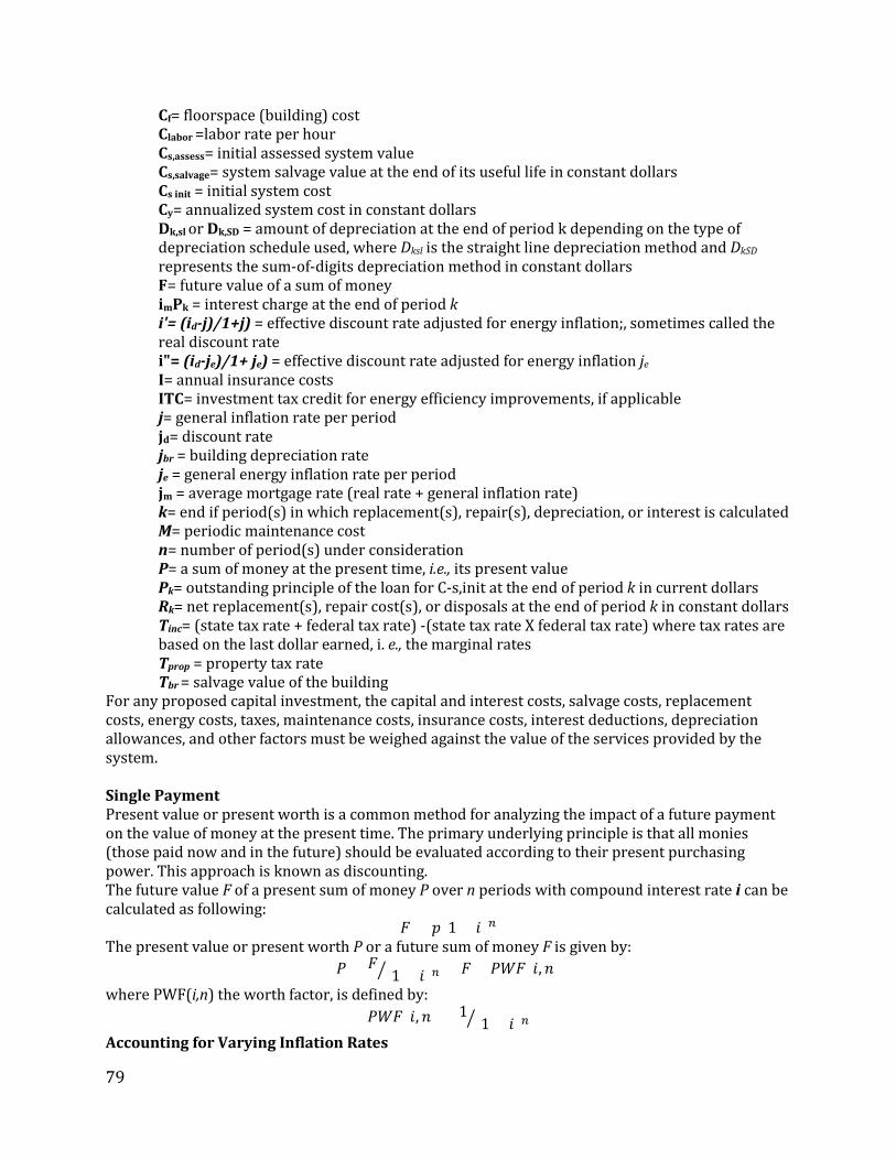
79

Cf= floorspace (building) cost Clabor =labor rate per hour Cs,assess= initial assessed system value Cs,salvage= system salvage value at the end of its useful life in constant dollars Cs init = initial system cost Cy= annualized system cost in constant dollars Dk,sl or Dk,SD = amount of depreciation at the end of period k depending on the type of depreciation schedule used, where Dksl is the straight line depreciation method and DkSD represents the sum-of-digits depreciation method in constant dollars F= future value of a sum of money imPk = interest charge at the end of period k i'= (id-j)/1+j) = effective discount rate adjusted for energy inflation;, sometimes called the real discount rate i"= (id-je)/1+ je) = effective discount rate adjusted for energy inflation je I= annual insurance costs ITC= investment tax credit for energy efficiency improvements, if applicable j= general inflation rate per period jd= discount rate jbr = building depreciation rate je = general energy inflation rate per period jm = average mortgage rate (real rate + general inflation rate) k= end if period(s) in which replacement(s), repair(s), depreciation, or interest is calculated M= periodic maintenance cost n= number of period(s) under consideration P= a sum of money at the present time, i.e., its present value Pk= outstanding principle of the loan for C-s,init at the end of period k in current dollars Rk= net replacement(s), repair cost(s), or disposals at the end of period k in constant dollars Tinc= (state tax rate + federal tax rate) -(state tax rate X federal tax rate) where tax rates are based on the last dollar earned, i. e., the marginal rates Tprop = property tax rate Tbr = salvage value of the building

For any proposed capital investment, the capital and interest costs, salvage costs, replacement costs, energy costs, taxes, maintenance costs, insurance costs, interest deductions, depreciation allowances, and other factors must be weighed against the value of the services provided by the system. Single Payment Present value or present worth is a common method for analyzing the impact of a future payment on the value of money at the present time. The primary underlying principle is that all monies (those paid now and in the future) should be evaluated according to their present purchasing power. This approach is known as discounting. The future value F of a present sum of money P over n periods with compound interest rate i can be calculated as following:

𝐹𝐹 = 𝑝𝑝(1 + 𝑖𝑖)𝑛𝑛 The present value or present worth P or a future sum of money F is given by:

𝑃𝑃 = 𝐹𝐹(1 + 𝑖𝑖)𝑛𝑛� = 𝐹𝐹 × 𝑃𝑃𝑃𝑃𝐹𝐹(𝑖𝑖,𝑛𝑛)

where PWF(i,n) the worth factor, is defined by: 𝑃𝑃𝑃𝑃𝐹𝐹(𝑖𝑖, 𝑛𝑛) = 1

(1 + 𝑖𝑖)𝑛𝑛� Accounting for Varying Inflation Rates

80

Inflation is another important economic parameter which accounts for the rise in costs of a commodity over time. Inflation must often be accounted for in an economic evaluation. One way to account for this is to use effective interest rates that account for varying rates of inflation. The effective interest rate i', sometimes called the real rate, accounts for the general inflation rate j and the discount rate 𝑗𝑗𝑑𝑑 , and can be expressed as follows (Haberl 1994). ):

𝑖𝑖′=1+𝑗𝑗𝑑𝑑1+𝑗𝑗 −1=𝑗𝑗𝑑𝑑−𝑗𝑗1+𝑗𝑗

However, this expression can be adapted to account for energy inflation by considering the general discount rate 𝑗𝑗𝑑𝑑and the energy inflation rate je, thus:

𝑖𝑖′′=1+𝑗𝑗𝑑𝑑1+𝑗𝑗𝑒𝑒−1=𝑗𝑗𝑑𝑑−𝑗𝑗𝑒𝑒1+𝑗𝑗𝑒𝑒

When considering the effects of varying inflation rates, the above discount equations can be revised to get the following equation for the future value F, using constant currency of an invested sum P with a discount rate 𝑗𝑗𝑑𝑑 under inflation j during n periods:

𝐹𝐹 = 𝑃𝑃[1 + 𝑗𝑗𝑑𝑑1 + 𝑗𝑗

]𝑛𝑛 = 𝑃𝑃(1 + 𝑖𝑖′)𝑛𝑛

The present worth P, in constant dollars, of a future sum of money F with discount rate 𝑗𝑗𝑑𝑑 under inflation rate j during n periods is then expressed as:

𝑃𝑃 = 𝐹𝐹/[1 + 𝑗𝑗𝑑𝑑1 + 𝑗𝑗

]𝑛𝑛

In constant currency, the present worth P of a sum of money F can be expressed with an effective interest rate 𝑖𝑖′, which is adjusted for inflation by:

𝑃𝑃 = 𝐹𝐹(1 + 𝑖𝑖′)𝑛𝑛� = 𝐹𝐹 × 𝑃𝑃𝑃𝑃𝐹𝐹(𝑖𝑖′,𝑛𝑛)

where the effective present worth factor is given by: 𝑃𝑃𝑃𝑃𝐹𝐹(𝑖𝑖′,𝑛𝑛) = 1

(1 + 𝑖𝑖′)𝑛𝑛�

Recovering Capital as a Series of Payments Another important economic concept is the recovery of capital as a series of uniform payments or what so called - the capital recovery factor (CRF). CRF is commonly used to describe periodic uniform mortgage or loan payments and S is defined as the ratio of the periodic payment to the total sum being repaid. The discounted sum S of such an annual series of payments Pann invested over n periods with interest rate i is given by:

𝑆𝑆 = 𝑃𝑃𝑎𝑎𝑛𝑛𝑛𝑛[1 + (1 + 𝑖𝑖)−𝑛𝑛/𝑖𝑖 𝑃𝑃𝑎𝑎𝑛𝑛𝑛𝑛 = (𝑆𝑆 × 𝑖𝑖)/[1 + (1 + 𝑖𝑖)−𝑛𝑛/𝑖𝑖

𝐶𝐶𝐶𝐶𝐹𝐹(𝑖𝑖,𝑛𝑛) =𝑖𝑖

[1 − (1 + 𝑖𝑖)−𝑛𝑛]=

𝑖𝑖(1 + 𝑖𝑖)𝑛𝑛

(1 + 𝑖𝑖)𝑛𝑛 − 1

Table A.2 below summarizes some of the mathematical formulas used in calculating these cost components.

(𝐶𝐶𝐶𝐶𝐹𝐹𝑖𝑖,𝑖𝑖𝑛𝑛𝑖𝑖𝑖𝑖 − 𝐼𝐼𝐼𝐼𝐶𝐶)𝐶𝐶𝐶𝐶𝐹𝐹(𝑖𝑖′,𝑛𝑛) Capital and Interest

(𝐶𝐶𝑠𝑠,𝑠𝑠𝑠𝑠𝑠𝑠𝑃𝑃𝑃𝑃𝐹𝐹(𝑖𝑖′,𝑛𝑛)𝐶𝐶𝐶𝐶𝐹𝐹(𝑖𝑖′,𝑛𝑛)(1 − 𝐼𝐼𝑠𝑠𝑎𝑎𝑠𝑠𝑠𝑠) Salvage Value

�[𝐶𝐶𝑘𝑘𝑃𝑃𝑃𝑃𝐹𝐹(𝑖𝑖′,𝑘𝑘)]𝑛𝑛

𝑘𝑘=1

𝐶𝐶𝐶𝐶𝐹𝐹(𝑖𝑖′,𝑛𝑛)( 1 − 𝐼𝐼𝑖𝑖𝑛𝑛𝑖𝑖) Replacement or Disposal

𝐶𝐶𝑒𝑒[𝐶𝐶𝐶𝐶𝐹𝐹�𝑖𝑖′,𝑛𝑛�𝐶𝐶𝐶𝐶𝐹𝐹�𝑖𝑖′′,𝑛𝑛�

](1− 𝐼𝐼𝑖𝑖𝑛𝑛𝑖𝑖) Operating Energy

Cbr = 𝐶𝐶𝐶𝐶𝐹𝐹𝑚𝑚 × 𝑐𝑐𝑓𝑓𝑠𝑠 × 𝑎𝑎𝑏𝑏𝑏𝑏 Building Cost

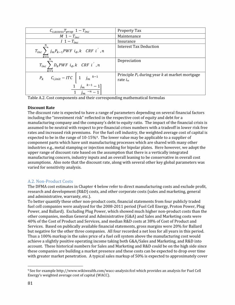
81

𝐶𝐶𝑠𝑠,𝑎𝑎𝑠𝑠𝑠𝑠𝑒𝑒𝑠𝑠𝑠𝑠𝐼𝐼𝑝𝑝𝑏𝑏𝑝𝑝𝑝𝑝(1 − 𝐼𝐼𝑖𝑖𝑛𝑛𝑖𝑖) Property Tax 𝑀𝑀(1 − 𝐼𝐼𝑖𝑖𝑛𝑛𝑖𝑖) Maintenance 𝐼𝐼(1 − 𝐼𝐼𝑖𝑖𝑛𝑛𝑖𝑖) Insurance

𝐼𝐼𝑖𝑖𝑛𝑛𝑖𝑖�[𝑗𝑗𝑚𝑚𝑃𝑃𝑘𝑘−1𝑃𝑃𝑃𝑃𝐹𝐹(𝑖𝑖𝑑𝑑 ,𝑘𝑘)]𝑛𝑛

𝑘𝑘=1

𝐶𝐶𝐶𝐶𝐹𝐹(𝑖𝑖′,𝑛𝑛) Interest Tax Deduction

𝐼𝐼𝑖𝑖𝑛𝑛𝑖𝑖�𝐷𝐷𝑘𝑘𝑃𝑃𝑃𝑃𝐹𝐹(𝑖𝑖𝑑𝑑 ,𝑘𝑘)]𝑛𝑛

𝑘𝑘=1

𝐶𝐶𝐶𝐶𝐹𝐹(𝑖𝑖′,𝑛𝑛) Depreciation

𝑃𝑃𝑘𝑘 = (𝐶𝐶𝑖𝑖,𝑖𝑖𝑛𝑛𝑖𝑖𝑖𝑖 − 𝐼𝐼𝐼𝐼𝐶𝐶) �(1 + 𝑗𝑗𝑚𝑚)𝑘𝑘−1

+(1 + 𝑗𝑗𝑚𝑚)𝑘𝑘−1 − 1(1 + 𝑗𝑗𝑚𝑚)−𝑛𝑛 − 1

�

Principle Pk during year k at market mortgage rate im

Table A.2. Cost components and their corresponding mathematical formulas Discount Rate The discount rate is expected to have a range of parameters depending on several financial factors including the “investment risk” reflected in the respective cost of equity and debt for a manufacturing company and the company’s debt to equity ratio. The impact of the financial crisis is assumed to be neutral with respect to pre-financial crises numbers with a tradeoff in lower risk free rates and increased risk premiums. For the fuel cell industry, the weighted average cost of capital is expected to be in the range of 10-15%9. The lower value may be applicable to a supplier of component parts which have unit manufacturing processes which are shared with many other industries e.g., metal stamping or injection molding for bipolar plates. Here however, we adopt the upper range of discount rate based on the assumption that there is a vertically integrated manufacturing concern, industry inputs and an overall leaning to be conservative in overall cost assumptions. Also note that the discount rate, along with several other key global parameters was varied for sensitivity analysis.

A.2. Non-Product Costs The DFMA cost estimates in Chapter 4 below refer to direct manufacturing costs and exclude profit, research and development (R&D) costs, and other corporate costs (sales and marketing, general and administrative, warranty, etc.). To better quantify these other non-product costs, financial statements from four publicly traded fuel cell companies were analyzed for the 2008-2011 period (Fuel Cell Energy, Proton Power, Plug Power, and Ballard). Excluding Plug Power, which showed much higher non-product costs than the other companies, median General and Administrative (G&A) and Sales and Marketing costs were 40% of the Cost of Product and Services, and median R&D costs at 38% of Cost of Product and Services. Based on publically available financial statements, gross margins were 20% for Ballard but negative for the other three companies. All four recorded a net loss for all years in this period. Thus a 100% markup in the sales price of a fuel cell system above the manufacturing cost would achieve a slightly positive operating income taking both G&A/Sales and Marketing, and R&D into account. These historical numbers for Sales and Marketing and R&D could be on the high side since these companies are building a market presence and these costs can be expected to drop over time with greater market penetration. A typical sales markup of 50% is expected to approximately cover

9 See for example http://www.wikiwealth.com/wacc-analysis:fcel which provides an analysis for Fuel Cell Energy’s weighted average cost of capital (WACC).

82

the G&A/Sales portion of operating expenses for current fuel cell vendors but not R&D expenses. Government policies or incentives could possibly mitigate the R&D expenses portion in some years. Gross margin product markup is also expected to be extremely slim given the existence of highly cost competitive alternative technologies for CHP applications and borne out by the financial data above. These other factors can be seen to increase the direct manufacturing costs by 50% to 100% including profit margin and can be taken as a sensitivity factor in the use-phase model chapter. Note that fuel cell system shipping and delivery costs are not split out separately, but that there is an additional 33% markup assumed for installation costs and all other fees.

A.3. Manufacturing Cost Analysis - Shared Parameters Shared parameters for the cost analysis are summarized below. Table A.3 shows the cell and stack configurations for CHP system based on the functional specifications described above. The number of cells per system will be used to compute total active area and component volumes in the DFMA section below. Similarly, the plate area and GDE coated area are shown in Table A.4. These cell areas could be expected to change for different applications for optimized product configuration and performance, but at the same time, it is beneficial for manufacturing cost control to have a consolidated cell size in multiple products and that approach was taken here.

System Power [kWe]

Cells/ stack

Stacks Cells/ system

Single cell power [W]

Gross Power [kWe]

1 21 1 21 60.9 1.28 10 105 2 210 60.0 12.6 50 131 8 1048 59.7 62.6 100 136 15 2040 59 121 250 136 38 5168 59.2 305.8

Table A.3. Summary of cell and stack configuration for CHP systems with reformate fuel. The number of cells per system is used to compute active areas and component volumes in the DFMA section below.

Parameter CHP HT PEM fuel cell Unit

Total plate area 720 cm2 GDE coated area 464 cm2

Table A.4. Plate and GDE coated area for CHP HT PEM fuel cell system. The former is an input for calculations of plate manufacturing costs and the latter for the membrane and GDE costing analysis. Parameter Symbol Value Units Comments Operating hours 𝑡𝑡ℎ𝑠𝑠 varies Hours 8 hours base shift; [1,1.5,2] shifts Annual Operating Days

𝑡𝑡𝑑𝑑𝑑𝑑 250 Days 52wks*5days/wk-10 vacation days

Production Availability

𝐴𝐴𝑚𝑚 0.85 Typical value in practice

Avg. Inflation Rate 𝑗𝑗 0.026 US avg. for past 10 years‡ Avg. Mortgage Rate 𝑗𝑗𝑚𝑚 0.05 See following reference ‡‡‡‡ Discount Rate 𝑗𝑗𝑑𝑑 0.15 Per Ballard (suggested >=15%)‡‡ Energy Inflation Rate 𝑗𝑗𝑒𝑒 0.056 US avg of last 3 years‡‡‡

83

Income Tax 𝑖𝑖𝑖𝑖 0 No net income Property Tax 𝑖𝑖𝑝𝑝 0.014 US avg from 2007† Assessed Value 𝑖𝑖𝑎𝑎𝑠𝑠 0 Salvage Tax 𝑖𝑖𝑠𝑠 0 EOL Salvage Value 𝑘𝑘𝑒𝑒𝑝𝑝𝑠𝑠 0.02 Assume 2% of end-of-life value Tool Lifetime 𝐼𝐼𝑖𝑖 15 Years Typical value in practice Energy Tax Credits 𝐼𝐼𝐼𝐼𝐶𝐶 0 Dollars Energy Cost 𝑐𝑐𝑒𝑒 0.1 $/kWhe Typical U.S. value Floor space Cost 𝑐𝑐𝑓𝑓𝑠𝑠 1291 $/m2 US average for factory†† Building Depreciation

𝑗𝑗𝑏𝑏𝑏𝑏 0.031 BEA rates† ††

Building Recovery 𝐼𝐼𝑏𝑏𝑏𝑏 31 Years BEA rates† †† Building Footprint 𝑎𝑎𝑏𝑏𝑏𝑏 Varies m2 Line Speed vl Varies m/min Approximation from DTI2010 (James et al.,

2010) Web Width W Varies M Lower widths at low volume Hourly Labor Cost 𝑐𝑐𝑠𝑠𝑎𝑎𝑏𝑏𝑝𝑝𝑏𝑏 28.08 $/hr Hourly wage per worker ‡ http://www.tradingeconomics.com/united-states/inflation-cpi ‡‡ Communications with Ballard Power Systems, Burnaby, B.C., Canada ‡‡‡ http://www.forecast-chart.com/inflation-usa-energy.html ‡‡‡‡ http://www.steelheadcapital.com/rates/ † http://www.nytimes.com/2007/04/10/business/11leonhardt-avgproptaxrates.html?_r=0 †† Selinger, B., (2011), “Building Costs,” DCEO, Illinois. ††† http://www.bea.gov/scb/account_articles/national/wlth2594/tableC.htm Table A.5. Manufacturing cost shared parameters. Manufacturing cost shared parameters are summarized in Table A.5. References are shown in the table and are a mixture of general industry numbers (e.g. annual operating days, inflation rate, tool lifetime) together with fuel cell specific industry assumptions (discount rate, web width, hourly wage).

An annualized cost of tool approach is adopted from Haberl (1994). The annualized cost equation and components are as follows:

Cy = Cc + Cr + Coc + Cp + Cbr + Ci + Cm − Cs − Cint − Cdep

where

Cy is the total annualized cost Cc is the capital/system cost (with interest) Cr is the replacements or disposal cost Coc is the operating costs (e.g. electricity) excluding labor Cp is the property tax cost Cbr is the building or floor space cost Ci is the tool insurance cost Cm is the maintenance cost Cs is the end-of-life salvage value Cint is the deduction from income tax Cdep is the deduction due to tool depreciation

Furthermore, all values are scaled to 2013 dollars. In the current version of the model Cr, the replacements or disposal cost and Ci, the tool insurance cost, are assumed to be zero. We assume no net income for fuel cell manufacturers, as is currently the case for LT PEM manufacturers and thus income tax credits such as interest tax credits do not factor into the calculations. The machine

84

rate quoted above can be easily found from these annualized cost components (capital cost component, operating cost, and building cost).

A.4. Factory model Two approaches were pursued: a global factory model with total area dependent on overall volume and including factors for non-production factory space, and secondly by incrementally adding factory area to each specific process module. It was found difficult to keep all modules coordinated in the first case, so later in the work, the factory costing shifted to the second, simpler approach. Factory cost contributions in both cases are found to be very small factors in general, especially as production volumes exceed 1000 systems per year.

A.5. Yield Considerations As in other costing studies (James 2012) and as will be detailed in the DFMA analysis below, this work assumes that high yield is achieved at high manufacturing volumes. This stems from several implicit assumptions:

• Learning by doing over the cumulative volume of fuel cell component production and greater process optimization will drive yield improvement both within a given vendor, and from vendor to vendor through industry interactions (conferences, IP, cross vendor personnel transfers, etc.)

• Inline inspection improvement with greater inspection sensitivity and more accurate response to defects and inline signals.

• Greater development and utilization of “transfer functions” (Manhattan Projection 2011), e.g., development of models that relate inline metrics and measurements to output responses and performance, and resultant improvement in inline response sensitivity and process control

• Utilization of greater feedback systems in manufacturing processing such as feed-forward sampling, for real time adjustment of process parameters (for example, slot die coating thickness and process parameter control).

• Systematic, integrated analysis to anticipate and prepare for yield excursions e.g., FMEA (failure modes and effect analysis).

Consideration of yield limiting mechanisms or FMEA-type analysis as a function of process tooling assumptions are out of scope here and would be very challenging in this type of analysis project without access to manufacturing data.

A.6. Initial Tool Sizing The choice of initial tool sizing was governed by several factors. In some cases it was made on the basis of tool availability and in other cases it was dependent on the choice of batch sizes with smaller batch sizes leading to smaller tools. In general however, tooling decisions were made to support medium to high volume manufacturing of greater than 10 kWe and 1,000 systems per year. This choice was made on the basis of assuming that vertically integrated manufacturing would not be done for small volumes e.g. 100 kWe of total production a year. A cost optimized process for low volume manufacturing would have a very different mix of automated versus manual production lines as well as in-house manufactured versus purchased components. Nor was a detailed optimization study of low volume manufacturing a key priority for this work. Production volumes might also be expected to grow if sales of fuel-cell vehicles drive increased demand for fuel cell stack components.

85

A.7. Time-frame for Cost Analysis The cost analysis utilizes largely existing manufacturing equipment technologies and existing materials with key exceptions noted (e.g., injection molding composite material for bipolar plates). It does not assume new high-speed manufacturing processes nor major fuel-cell technology advances such as much lower cost catalysts or membranes. The analysis is thus a “potential cost reduction” study for future costs with existing tools and mostly existing materials. The study assumes that higher overall volumes will drive significant improvements in yield, but it is not a market adoption or market penetration study and therefore timelines will vary according to the assumptions made for market adoption. Stationary fuel cell systems may also benefit from growth in the transportation sector and higher volumes achieved for fuel cell components in that sector over the next few years may reduce the cost of components for stationary applications (e.g., GDE, membranes, metal plates, etc.).

86

Appendix B: DFMA Manufacturing Cost Analysis

B.1. Polybenzimidazol88 (PBI) based membranes Stack parameters and assumptions Stack parameters and assumptions for a 100kW HT PEMFC system are shown in Table B.1 below. Line utilization is seen to be low until the 10000 systems per year manufacturing level. Note that line utilization applies to all process modules, since the process flow is a continuous process.

Power (kW) 100 Lines 1 1 7 29 Stacks/Yr 100 1,000 10,000 50,000 Scrap 14% 10% 7% 6% Overall Yield 86% 90% 93% 94% Line Speed (m/s) 0.0067 0.0100 0.0100 0.0100 Line Speed (m/min) 0.4 0.6 0.6 0.6 Line Utilization 20.05% 73.59% 85.65% 99.42% Number of MEA cells 2040 2040 2040 2040

Membrane Actual Area (m2) 9.46E+03 9.46E+04 9.46E+05 4.73E+06 Membrane Used Area (m2) 1.10E+04 1.05E+05 1.02E+06 5.03E+06 Web Width (m) 0.54 0.90 0.90 0.90 No of Rolls 110 1051 10168 50295 Installation factor 1.10 1.10 1.10 1.10 Avg. Availability 0.85 0.85 0.98 0.99 Max Annual Area (m2) 63769.42 158630.40 1276387.44 5381850.89

Annual Operation Hours (No setup)

981.55 3602.88 4820.27 5694.44

Annual Operation Hours (+setup time)

1052.55 3860.88 5165.27 6101.44

Machine/Worker 2 2 8 30 Worker Rate 29.81 29.81 29.81 29.81 Slot-die Machine Footprint 40.61 40.61 284.25 1177.59

Table B.1. Stack parameters and assumptions for a 100kW system.

Module Total Cost

Slot Die coater $723,000 IR Oven $180,000 Mixing and Pumping System 102,000 Quality Control System $175,000 Wind/Unwind System $170,000

87

Viscometer (not included in Conquip quote) $6,000

Installation $135,600 Total $1,491,600

Table B.2. Overall Process Equipment Cost by Module for slot die casting machine. Machine Rates by Module Machine rates for the slot-die coater are shown below for the 100kW base system. Slot-Die Coater and IR oven: Some important assumptions for slot-die coater are:

• Maintenance factor per James et al., (2010) • Power consumption (5kW for slot-die coater and 50kW for IR oven based on machine

specifications from EuroTech.) • Machine footprint based on web width and line length and assumed cleanroom 1000 class

for slot die-coater and IR oven. • Initial system cost assumes installation costs are 10% of capital cost (based on EuroTech &

Conquip estimates) • Salvage value is the amortized end-of-life value of the tool. • Property tax is proportional to the machine capital.

Systems/yr 100 1,000 10,000 50,000 Line Speed (m/min) 0.402 0.600 0.600 0.600 Maintenance factor 0.10 0.10 0.10 0.10 Auxiliary Costs Factor 0 0 0 0 Power Consumption (kW) 5 5 5 5 Machine Footprint (m2) 20.40 20.40 142.80 591.60 Initial Capital 723000 723000 5061000 20967000 Initial System Cost 795300 795300 5567100 23063700 Annual Depreciation 47236 47236 330652 1369844 Annual Cap Payment 117304.55 117304.55 821131.87 3401832.05 Auxiliary Costs 0 0 0 0 Maintenance 10664.05 10664.05 74648.35 309257.46 Salvage Value 1305.81 1305.81 9140.69 37868.59 Energy Costs 1258.72 4617.12 43239.02 211600 Property Tax 3990.96 3990.96 27936.72 115737.84 Building Costs 1640.53 1640.53 11483.72 47575.41 Machine Rate ($/hr) 126.89 35.46 187.66 663.47

Capital ($/hr) 110.21 30.04 157.20 551.34 Variable ($/hr) 11.33 3.96 22.82 85.37 Building ($/hr) 5.35 1.46 7.63 26.77

Table B.3. Machine rates for slot-die coater.

88

Systems/yr 100 1,000 10,000 50,000 Line Speed (m/min) 0.402 0.600 0.600 0.600 Maintenance factor 0.10 0.10 0.10 0.10 Auxiliary Costs Factor 0 0 0 0 Power Consumption (kW) 50.00 50.00 50.00 50.00 Machine Footprint (m2) 20.40 20.40 142.80 591.60 Initial Capital 180000 180000 1260000 5220000 Initial System Cost 198000 198000.00 1386000 5742000 Annual Depreciation 11760 11760 82320 341040 Annual Cap Payment 29204.45 29204.45 204431.17 846929.14 Auxiliary Costs 0 0 0 0 Maintenance 2654.95 2654.95 18584.65 76993.56 Salvage Value 325.10 325.10 2275.69 9427.86 Energy Costs 12587.15 46171.24 432390.20 2115999.99 Property Tax 993.60 993.60 6955.20 28814.40 Building Costs 3281.06 3281.06 22967.44 95150.81 Machine Rate ($/hr) 45.98 21.23 132.24 517.00

Capital ($/hr) 27.44 7.48 39.14 137.26 Variable ($/hr) 14.48 12.65 87.31 359.42 Building ($/hr) 4.06 1.11 5.79 20.32

Table B.4. Machine rates for IR oven.

Systems/yr 100 1,000 10,000 50,000 Maintenance factor 0.10 0.10 0.10 0.10 Auxiliary Costs Factor 0 0 0 0 Power Consumption (kW) 4.00 4.00 4.00 4.00 Machine Footprint (m2) 1.62 1.62 11.34 46.98 Initial Capital 102000 102000 714000 2958000 Initial System Cost 112200 112200 785400 3253800 Annual Depreciation 6664 6664 46648 193256 Annual Cap Payment 16549.19 16549.19 115844.33 479926.51 Auxiliary Costs 0 0 0 0 Maintenance 1504.47 1504.47 10531.30 43629.68 Salvage Value 184.22 184.22 1289.56 5342.46 Energy Costs 503.49 1846.85 17295.61 84640.00 Property Tax 563.04 563.04 3941.28 16328.16 Building Costs 1093.69 1093.69 7655.81 31716.94 Machine Rate ($/hr) 19.03 5.54 29.81 106.68

Capital ($/hr) 15.55 4.24 22.18 77.78

89

Variable ($/hr) 1.91 0.87 5.39 21.02 Building ($/hr) 1.57 0.43 2.25 7.87

Table B.5. Machine rate of the Mixing and Pumping System

Systems/yr 100 1,000 10,000 50,000 Maintenance factor 0.10 0.10 0.10 0.10 Auxiliary Costs Factor 0 0 0 0 Power Consumption 15.00 15.00 15.00 15.00 Machine Footprint (m2) 9.72 16.20 113.40 469.80 Initial Capital 181000 181000 1267000 5249000 Initial System Cost 199100 199100 1393700 5773900 Annual Depreciation 11825.33 11825.33 82777.33 342934.67 Annual Cap Payment 29366.70 29366.70 205566.90 851634.30 Auxiliary Costs 0 0 0 0 Maintenance 2669.70 2669.70 18687.90 77421.30 Salvage Value 980.71 980.71 6865.00 28440.72 Energy Costs 5664.22 20777.06 194575.59 952200.00 Property Tax 999.12 999.12 6993.84 28974.48 Building Costs 1640.53 1640.53 11483.72 47575.41 Machine Rate ($/hr) 37.39 14.11 83.33 316.21

Capital ($/hr) 26.97 7.35 38.47 134.92 Variable ($/hr) 7.92 6.07 41.29 168.75 Building ($/hr) 2.51 0.68 3.58 12.55

Table B.6. Machine rate of the Quality Control Unit (XRF or Optical Unit)+ Viscosity Meter

Systems/yr 100 1,000 10,000 50,000 Maintenance factor 0.10 0.10 0.10 0.10 Auxiliary Costs Factor 0 0 0 0 Power Consumption 10.00 10.00 10.00 10.00 Machine Footprint (m2) 3.00 3.00 21.00 87.00 Initial Capital 170000.00 170000.00 1190000.00 4930000.00 Initial System Cost 187000.00 187000.00 1309000.00 5423000.00 Annual Depreciation 11106.67 11106.67 77746.67 322093.33 Annual Cap Payment 27581.98 27581.98 193073.88 799877.52 Auxiliary Costs 0 0 0 0 Maintenance 2507.45 2507.45 17552.17 72716.14 Salvage Value 307.04 307.04 2149.26 8904.09 Energy Costs 1258.72 4617.12 43239.02 211600.00 Property Tax 938.40 938.40 6568.80 27213.60

90

Building Costs 2920.15 2920.15 20441.02 84684.22 Machine Rate ($/hr) 33.16 9.91 53.96 194.57

Capital ($/hr) 25.91 7.06 36.96 129.64 Variable ($/hr) 3.58 1.85 11.77 46.60 Building ($/hr) 3.67 1.00 5.23 18.34

Table B.7. Machine rate of the Wind/Unwind Tensioners

Systems/yr 100 1,000 10,000 50,000 Lines 1 5 43 210 Adjusted No. of lines 1 1 3 11 Maintenance factor 0.10 0.10 0.10 0.10 Auxiliary Costs Factor 0 0 0 0 Required doping time (days) 110 240 240 240 Power Consumption (kW) 5 5 15 55 Machine Footprint (m2) 30.00 150.00 1290.00 6300.00 Initial Capital 36000 36000 108000 396000 Initial System Cost 39600 39600 118800 435600 Annual depreciation 2352.00 2352.00 7056.00 25872.00 Annual Cap Payment 5840.89 5840.89 17522.67 64249.80 Auxiliary Costs 0 0 0 0 Maintenance 530.99 530.99 1592.97 5840.89 Salvage Value 65.02 65.02 195.06 715.22 Energy Costs 1578.55 3444.12 30997.04 416737.92 Property Tax 198.72 198.72 596.16 2185.92 Building Costs 10575.96 10575.96 74031.71 306702.79 Machine Rate ($/hr) 17.73 5.32 24.11 130.30

Capital ($/hr) 5.49 1.50 3.35 10.41 Variable ($/hr) 2.00 1.03 6.31 69.26 Building ($/hr) 10.24 2.79 14.45 50.63

Table B.8. Machine rate of the doping station

Gas Diffusion Electrodes Ink preparation method Ink preparation method based on UTC patent (US patent #4,613,582) is described briefly here. A precise amount of the commercially available high surface area platinum-on-graphitized-carbon-black (containing 10% platinum by weight) is dispersed in distilled water followed by ultrasonic blending for about 15 minutes. The pH should be monitored and adjusted to about 8 with dilute ammonium hydroxide solution to aid in the dispersion of the supported catalyst. Continuous stirring is necessary to ensure uniformity of the solution/slurry at all times. After that a solution of ammonium chromate dissolved in water is then added to the pH-adjusted solution. Following this addition the pH should be maintained around 5.5 by addition of dilute hydrochloric acid to facilitate

91

adsorption of the chromium onto the platinum. The solution is then stirred, to intimately contact the platinum-on-graphitized-carbon black and the chromium salt, for about 15 minutes. A separate solution of cobaltous nitrate in distilled water is then added to the above acidic solution. Both the ammonium chromate and cobaltous nitrate are added as solutions to enhance the dispersion of these metals onto the catalyst, while the stirring brings the metals into the intimate contact required for proper adsorption onto the supported platinum catalyst. The pH should be maintained at about 5.5 by incremental additions of dilute hydrochloric acid. Stirring is employed during this procedure and continued for about 15 minutes after the addition, to intimately contact all the constituents. After that the solid is dried at about 90° C. and sifted through an 80 mesh screen. The sifted solids were then heat treated at about 900°C in controlled nitrogen-rich environment for 1 hour to form the platinum chromium-cobalt alloy catalyst. The catalyst prepared according to this method, which showed an increase in catalytic activity should have a metallic composition comprising cobalt 11.3% by weight, chromium 8.9% by weight with the balance being platinum for optimal conductivity and performance. Machine Rates for GDE Coating Process

Power (kW) 100 Lines 1 1 3 13 Systems/Yr 100 1000 10000 50000 Scrap 4% 0.030 0.020 0.010 Overall Yield 96.00% 97.00% 98.00% 99.00% Line Utilization 5.05% 49.49% 87.02% 94.37% Number of MEA cells 2040 2040 2040 2040 GDE Actual Area (m2) 18910.80 189108.00 1891080.00 9455400.00 GDE Area (m2) 24623.44 243695.88 2412091.84 11938636.36 Web Width (m) 0.54 0.54 0.90 0.90 Power density (kW/m2) 4.39 4.39 4.39 4.39 Theoritical Membrane area (m2)

2277.90 22779.04 227790.43 1138952.16

% of inactive area 10% 10% 10% 10%

% of scrap rate 10% 10% 10% 10% Actual GDE Area (m2) 2.81E+03 2.81E+04 2.81E+05 1.41E+06 Installation factor 1.10 1.10 1.10 1.10 Avg. Availability 0.85 0.85 0.95 0.99 Max Annual Area (m2) 6.35E+05 6.35E+05 3.54E+06 1.60E+07 Annual Operation Hours (No setup)

131.94 1292.35 2532.22 2863.06

Annual Operation Hours (+setup time)

141.94 1385.35 2713.22 3068.06

Machine/Worker 2 2 6 26

Worker Rate 29.81 29.81 29.81 29.81

92

Machine Footprint 50.4 50.4 151.2 655.2 Table B.9. GDE coating line parameters and assumptions for a 100kW system.

Module Total Cost for slot-die coating line

Slot Die coater $1,521,000 IR Oven $360,000 Mixing and Pumping System 204000 Quality Control System $850,000 Wind/Unwind System $645,000 Viscometer (not included in Conquip quote) $6,000

Installation $390,000

Total $3,976,000 Table B.10. Overall Process Equipment Cost by Module for GDE coating line.

Systems/yr 100 1,000 10,000 50,000 Line Speed (m/min) 6 6 6 6 Maintenance factor 0.10 0.10 0.10 0.10 Auxiliary Costs Factor 0 0 0 0 Power Consumption 5 5 5 5 Machine Footprint (m2) 20.40 20.40 61.20 265.20 Initial Capital 723000 723000 2169000 9399000 Initial System Cost 795300 795300 2385900 10338900 Annual Depreciation 47236 47236 141708 614068 Annual Cap Payment 117304.55 117304.55 351913.66 1524959.20 Auxiliary Costs 0 0 0 0 Maintenance 10664.05 10664.05 31992.15 138632.65 Salvage Value 1305.81 1305.81 3917.44 16975.57 Energy Costs 169.74 1656.70 9734.00 47697.22 Property Tax 3990.96 3990.96 11972.88 51882.48 Building Costs 5083.90 5083.90 15251.69 66090.64 Machine Rate ($/hr) 957.49 99.18 153.67 590.69

Capital ($/hr) 817.23 83.73 128.26 491.51 Variable ($/hr) 76.33 8.89 15.38 60.73 Building ($/hr) 63.93 6.55 10.03 38.45

Table B.11. Machine rate of the Slot-die coater

93

Systems/yr 100 1,000 10,000 50,000 Line Speed (m/min) 6.0 6.0 6.0 6.0 Maintenance factor 0.10 0.10 0.10 0.10 Auxiliary Costs Factor 0.00 0.00 0.00 0.00 Power Consumption 50.00 50.00 50.00 50.00 Machine Footprint (m2) 20.40 20.40 61.20 265.20 Initial Capital 180000 180000 540000 2340000 Initial System Cost 198000 198000 594000 2574000 Annual Depreciation 11760 11760 35280 152880 Annual Cap Payment 29204.45 29204.45 87613.36 379657.89 Auxiliary Costs 0 0 0 0 Maintenance 2654.95 2654.95 7964.85 34514.35 Salvage Value 325.10 325.10 975.30 4226.28 Energy Costs 1697.44 16567.03 97340.03 476972.16 Property Tax 993.60 993.60 2980.80 12916.80 Building Costs 10167.79 10167.79 30503.37 132181.28 Machine Rate ($/hr) 312.76 42.78 83.08 336.37

Capital ($/hr) 203.46 20.85 31.93 122.37 Variable ($/hr) 30.66 13.88 38.81 166.71 Building ($/hr) 78.63 8.06 12.34 47.29

Table B.12. Machine rate of the Infrared Dryer Systems/yr 100 1,000 10,000 50,000 Maintenance factor 0.10 0.10 0.10 0.10 Auxiliary Costs Factor 0 0 0 0 Power Consumption (kW) 4 4 4 4 Machine Footprint (m2) 1.62 1.62 4.86 21.06 Initial Capital 102000 102000 306000 1326000 Initial System Cost 112200 112200 336600 1458600 Annual Depreciation 6664 6664 19992 86632 Annual Cap Payment 16549.19 16549.19 49647.57 215139.47 Auxiliary Costs 0 0 0 0 Maintenance 1504.47 1504.47 4513.42 19558.13 Salvage Value 184.22 184.22 552.67 2394.89 Energy Costs 67.90 662.68 3893.60 19078.89 Property Tax 563.04 563.04 1689.12 7319.52 Building Costs 5083.90 5083.90 15251.69 66090.64 Machine Rate ($/hr) 166.15 17.45 27.44 105.86

Capital ($/hr) 115.29 11.81 18.09 69.34 Variable ($/hr) 11.08 1.56 3.10 12.59

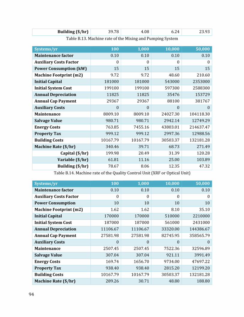
94

Building ($/hr) 39.78 4.08 6.24 23.93 Table B.13. Machine rate of the Mixing and Pumping System

Systems/yr 100 1,000 10,000 50,000 Maintenance factor 0.10 0.10 0.10 0.10 Auxiliary Costs Factor 0 0 0 0 Power Consumption (kW) 15 15 15 15 Machine Footprint (m2) 9.72 9.72 48.60 210.60 Initial Capital 181000 181000 543000 2353000 Initial System Cost 199100 199100 597300 2588300 Annual Depreciation 11825 11825 35476 153729 Annual Cap Payment 29367 29367 88100 381767 Auxiliary Costs 0 0 0 0 Maintenance 8009.10 8009.10 24027.30 104118.30 Salvage Value 980.71 980.71 2942.14 12749.29 Energy Costs 763.85 7455.16 43803.01 214637.47 Property Tax 999.12 999.12 2997.36 12988.56 Building Costs 10167.79 10167.79 30503.37 132181.28 Machine Rate ($/hr) 340.46 39.71 68.73 271.49

Capital ($/hr) 199.98 20.49 31.39 120.28 Variable ($/hr) 61.81 11.16 25.00 103.89 Building ($/hr) 78.67 8.06 12.35 47.32

Table B.14. Machine rate of the Quality Control Unit (XRF or Optical Unit)

Systems/yr 100 1,000 10,000 50,000 Maintenance factor 0.10 0.10 0.10 0.10 Auxiliary Costs Factor 0 0 0 0 Power Consumption 10 10 10 10 Machine Footprint (m2) 1.62 1.62 8.10 35.10 Initial Capital 170000 170000 510000 2210000 Initial System Cost 187000 187000 561000 2431000 Annual Depreciation 11106.67 11106.67 33320.00 144386.67 Annual Cap Payment 27581.98 27581.98 82745.95 358565.79 Auxiliary Costs 0 0 0 0 Maintenance 2507.45 2507.45 7522.36 32596.89 Salvage Value 307.04 307.04 921.11 3991.49 Energy Costs 169.74 1656.70 9734.00 47697.22 Property Tax 938.40 938.40 2815.20 12199.20 Building Costs 10167.79 10167.79 30503.37 132181.28 Machine Rate ($/hr) 289.26 30.71 48.80 188.80

95

Capital ($/hr) 192.16 19.69 30.16 115.57 Variable ($/hr) 18.86 3.01 6.36 26.17 Building ($/hr) 78.24 8.02 12.28 47.06

Table B.15. Machine rate of the Wind/Unwind Tensioners

MEA Frame/Seal

Power (kW) 100 Lines 1 4 33 163 Stacks/Yr 100 1,000 10,000 50,000 No. Cells 204000 2040000 20400000 102000000 Overall Yield 0.985 0.999 0.999 0.999 New Yield 0.7883 0.7992 0.7992 0.7992 Line Utilization 96.6% 84.4% 98.71% 99.53% Cycle time (min/part)

0.83 0.33 0.33 0.33

Configuration A B B B Installation factor 1.4 1.4 1.4 1.4 Avg. Availability 0.850 0.960 0.995 0.999 Annual Operation Hours

3382.85 11815.10 114006.86 567799.74

Frame Scrap 0.555 0.555 0.555 0.555 Setup Time (hrs) 0 0 0 0 Hours per shift 7 7 7 7 No. shifts 2 2 2 2 Workers per shift 1 3 9 22 Annual Worker hours

3500 10500 31500 77000

Worker Rate 28.08 28.08 28.08 28.08 Machine Footprint (m2)

42 168 1386 6846

Building Footprint 7400 18700 120300 561900 Leased Amount 0 0 0 0 Space Fraction 0.02196173 0.0579095 0.20583191 0.279832516 Building Cost 13466.17 89729.91 2051748.4 13028756.97 Table B.16. MEA frame/seal line parameters and assumptions for a 100kW system

Systems/yr 100 1,000 10,000 50,000 Cycle time 6 6 6 6

Maintenance factor 0.1 0.1 0.1 0.1 Auxiliary Costs Factor 0 0 0 0 Power Consumption 5 5 5 5

96

Initial Capital 63882.48 255529.92 2108121.84 10412844.24 Initial System Cost 89435.472 357741.888 2951370.58 14577981.94

Annual Depreciation 4173.65536 16694.6214 137730.627 680305.8237 Annual Cap Payment 12887.10 51548.41 425274.42 2100597.91

Auxiliary Costs 0 0 0 0 Maintenance 920.51 3682.03 30376.74 150042.71 Salvage Value 122.31 489.25 4036.33 19937.02 Energy Costs 201.56 1988.06 19880.63 99403.17 Property Tax 357.74 1430.97 11805.48 58311.93

Space Fraction 0 0 0 0 Building Costs 0 0 0 0

Machine Rate ($/hr) 4.21 4.92 4.24 4.21 Capital ($/hr) 3.88 4.44 3.80 3.77

Variable ($/hr) 0.33 0.48 0.44 0.44 Building ($/hr) 0.00 0.00 0.00 0.00

Table B.17. Machine Rate for the Membrane Roll

Systems/yr 100 1,000 10,000 50,000 Cycle time 6 6 6 6

Maintenance factor 0.1 0.1 0.1 0.1 Auxiliary Costs Factor 0 0 0 0 Power Consumption 5 5 5 5

Initial Capital 63882.48 255529.92 2108121.84 10412844.24 Initial System Cost 89435.472 357741.888 2951370.58 14577981.94

Annual Depreciation 4173.65536 16694.6214 137730.627 680305.8237 Annual Cap Payment 12887.10 51548.41 425274.42 2100597.91

Auxiliary Costs 0.00 0.00 0.00 0.00 Maintenance 920.51 3682.03 30376.74 150042.71 Salvage Value 122.31 489.25 4036.33 19937.02 Energy Costs 201.56 1988.06 19880.63 99403.17 Property Tax 357.74 1430.97 11805.48 58311.93

Space Fraction 0 0 0 0 Building Costs 0 0 0 0

Machine Rate ($/hr) 4.21 4.92 4.24 4.21 Capital ($/hr) 3.88 4.44 3.80 3.77

Variable ($/hr) 0.33 0.48 0.44 0.44 Building ($/hr) 0.00 0.00 0.00 0.00

Table B.18. Machine Rate for the GDE Anode Roll

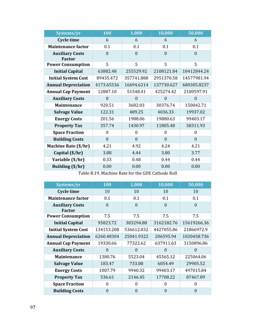
97

Systems/yr 100 1,000 10,000 50,000 Cycle time 6 6 6 6

Maintenance factor 0.1 0.1 0.1 0.1 Auxiliary Costs

Factor 0 0 0 0

Power Consumption 5 5 5 5 Initial Capital 63882.48 255529.92 2108121.84 10412844.24

Initial System Cost 89435.472 357741.888 2951370.58 14577981.94 Annual Depreciation 4173.65536 16694.6214 137730.627 680305.8237 Annual Cap Payment 12887.10 51548.41 425274.42 2100597.91

Auxiliary Costs 0 0 0 0 Maintenance 920.51 3682.03 30376.74 150042.71 Salvage Value 122.31 489.25 4036.33 19937.02 Energy Costs 201.56 1988.06 19880.63 99403.17 Property Tax 357.74 1430.97 11805.48 58311.93

Space Fraction 0 0 0 0 Building Costs 0 0 0 0

Machine Rate ($/hr) 4.21 4.92 4.24 4.21 Capital ($/hr) 3.88 4.44 3.80 3.77

Variable ($/hr) 0.33 0.48 0.44 0.44 Building ($/hr) 0.00 0.00 0.00 0.00

Table B.19. Machine Rate for the GDE Cathode Roll

Systems/yr 100 1,000 10,000 50,000 Cycle time 10 10 10 10

Maintenance factor 0.1 0.1 0.1 0.1 Auxiliary Costs

Factor 0 0 0 0

Power Consumption 7.5 7.5 7.5 7.5 Initial Capital 95823.72 383294.88 3162182.76 15619266.36

Initial System Cost 134153.208 536612.832 4427055.86 21866972.9 Annual Depreciation 6260.48304 25041.9322 206595.94 1020458.736 Annual Cap Payment 19330.66 77322.62 637911.63 3150896.86

Auxiliary Costs 0 0 0 0 Maintenance 1380.76 5523.04 45565.12 225064.06 Salvage Value 183.47 733.88 6054.49 29905.52 Energy Costs 1007.79 9940.32 99403.17 497015.84 Property Tax 536.61 2146.45 17708.22 87467.89

Space Fraction 0 0 0 0 Building Costs 0 0 0 0

98

Machine Rate ($/hr) 6.52 7.97 6.97 6.92 Capital ($/hr) 5.82 6.66 5.70 5.65

Variable ($/hr) 0.71 1.31 1.27 1.27 Building ($/hr) 0 0 0 0

Table B.20. Machine Rate for the Frame Roll

Systems/yr 100 1,000 10,000 50,000 Cycle time 15 15 15 15

Maintenance factor 0.15 0.15 0.15 0.15 Auxiliary Costs

Factor 0 0 0 0

Power Consumption 15 15 15 15 Initial Capital 90500.18 362000.72 2986505.94 14751529.34

Initial System Cost 126700.252 506801.008 4181108.32 20652141.08 Annual Depreciation 5912.67843 23650.7137 195118.388 963766.5835 Annual Cap Payment 18256.73 73026.92 602472.10 2975847.04

Auxiliary Costs 0 0 0 0 Maintenance 1956.08 7824.31 64550.58 318840.75 Salvage Value 173.28 693.11 5718.13 28244.10 Energy Costs 1511.68 14910.48 149104.75 745523.76 Property Tax 506.80 2027.20 16724.43 82608.56

Space Fraction 0 0 0 0 Building Costs 0 0 0 0

Machine Rate ($/hr) 6.52 8.22 7.26 7.21 Capital ($/hr) 5.50 6.29 5.38 5.34

Variable ($/hr) 1.03 1.92 1.87 1.87 Building ($/hr) 0 0 0 0

Table B.21. Machine Rate for the Robotic Arm

Systems/yr 100 1,000 10,000 50,000 Cycle time 20 20 20 20

Maintenance factor 0.15 0.15 0.15 0.15 Auxiliary Costs

Factor 0 0 0 0

Power Consumption 15 15 15 15 Initial Capital 106470.8 425883.2 3513536.4 17354740.4

Initial System Cost 149059.12 596236.48 4918950.96 24296636.56 Annual Depreciation 6956.09227 27824.3691 229551.045 1133843.039 Annual Cap Payment 21478.51 85914.02 708790.71 3500996.52

Auxiliary Costs 0 0 0 0

99

Maintenance 2301.27 9205.07 75941.86 375106.77 Salvage Value 203.85 815.42 6727.21 33228.36 Energy Costs 2015.58 19880.63 198806.34 994031.68 Property Tax 596.24 2384.95 19675.80 97186.55

Space Fraction 0 0 0 0 Building Costs 0 0 0 0

Machine Rate ($/hr) 7.74 9.87 8.74 8.69 Capital ($/hr) 6.47 7.40 6.33 6.28

Variable ($/hr) 1.28 2.46 2.41 2.41 Building ($/hr) 0 0 0 0

Table B.22. Machine Rate for the 7-axis Arm

Systems/yr 100 1,000 10,000 50,000 Cycle time 30 30 30 30

Maintenance factor 0.1 0.1 0.1 0.1 Auxiliary Costs

Factor 0 0 0 0

Power Consumption 17.5 17.5 17.5 17.5 Initial Capital 106470.8 851766.4 7027072.8 34709480.8

Initial System Cost 149059.12 1192472.96 9837901.92 48593273.12 Annual Depreciation 6956.09227 55648.7381 459102.09 2267686.079 Annual Cap Payment 21478.51 171828.05 1417581.41 7001993.03

Auxiliary Costs 0.00 0.00 0.00 0.00 Maintenance 1534.18 12273.43 101255.82 500142.36 Salvage Value 203.85 1630.84 13454.43 66456.72 Energy Costs 3527.26 34791.11 347911.09 1739555.44 Property Tax 596.24 4769.89 39351.61 194373.09

Space Fraction 0.000E+00 0.000E+00 0.000E+00 0.000E+00 Building Costs 0.00 0.00 0.00 0.00

Machine Rate ($/hr) 7.96 18.79 16.60 16.50 Capital ($/hr) 6.47 14.81 12.66 12.56

Variable ($/hr) 1.50 3.98 3.94 3.94 Building ($/hr) 0 0 0 0

Table B.23. Machine Rate for the Hot Press

Systems/yr 100 1,000 10,000 50,000 Cycle time 5 5 5 5

Maintenance factor 0.1 0.1 0.1 0.1 Auxiliary Costs

Factor 0 0 0 0

Power Consumption 10 10 10 10

100

Initial Capital 53235.4 212941.6 1756768.2 8677370.2 Initial System Cost 74529.56 298118.24 2459475.48 12148318.28

Annual Depreciation 3478.04613 13912.1845 114775.522 566921.5197 Annual Cap Payment 10739.25 42957.01 354395.35 1750498.26

Auxiliary Costs 0 0 0 0 Maintenance 767.09 3068.36 25313.95 125035.59 Salvage Value 101.93 407.71 3363.61 16614.18 Energy Costs 335.93 3313.44 33134.39 165671.95 Property Tax 298.12 1192.47 9837.90 48593.27

Space Fraction 0 0 0 0 Building Costs 0.00 0.00 0.00 0.00

Machine Rate ($/hr) 3.56 4.24 3.68 3.65 Capital ($/hr) 3.23 3.70 3.17 3.14

Variable ($/hr) 0.33 0.54 0.51 0.51 Building ($/hr) 0 0 0 0

Table B.24. Machine Rate for the Final Blank Press

Systems/yr 100 1,000 10,000 50,000 Cycle time 2 2 2 2

Maintenance factor 0.05 0.05 0.05 0.05 Auxiliary Costs

Factor 0 0 0 0

Power Consumption 2 2 2 2 Initial Capital 15970.62 63882.48 527030.46 2603211.06

Initial System Cost 22358.868 89435.472 737842.644 3644495.484 Annual Depreciation 1043.41384 4173.65536 34432.6567 170076.4559 Annual Cap Payment 3221.78 12887.10 106318.61 525149.48

Auxiliary Costs 0 0 0 0 Maintenance 115.06 460.25 3797.09 18755.34 Salvage Value 30.58 122.31 1009.08 4984.25 Energy Costs 26.87 265.08 2650.75 13253.76 Property Tax 89.44 357.74 2951.37 14577.98

Space Fraction 0 0 0 0 Building Costs 0 0 0 0

Machine Rate ($/hr) 1.01 1.17 1.01 1.00 Capital ($/hr) 0.97 1.11 0.95 0.94

Variable ($/hr) 0.04 0.06 0.06 0.06 Building ($/hr) 0 0 0 0

Table B.25. Machine Rate for the Unload MEA Tray

101

Sensitivity Analysis for Stack modules The impact of changing several parameters on the stack modules is calculated for a ±20% change in the sensitivity parameter being varied. Figures B.1 to B.4 show sensitivity analysis results expressed in $/kWe for PBI membrane, GDE, frame/seal and plates, respectively.

(a)

(b)

-15.00 -10.00 -5.00 0.00 5.00 10.00 15.00 20.00

Process Yield

Power Density

Capital

Discount Rate

Building Cost

100 kW @100 sys/yr Nominal Cost= $58.81/kW

"-20% "+20%

-4.00 -2.00 0.00 2.00 4.00 6.00 8.00 10.00

Process Yield

Power Density

Capital

Discount Rate

Building Cost

100 kW @1,000 sys/yr Nominal Cost= $21.59/kW

"-20% "+20%

102

(c)

(d)

Figure B.1. Sensitivity analysis plots for PBI-membrane. Plots show equivalent area for 100 kW system expressed in ($/kW) at different annual production rates: (a) 100 units/yr; (b) 1,000 units/yr; (c) 10,000 units /yr; and (d) 50,000 units/yr.

-4.00 -2.00 0.00 2.00 4.00 6.00 8.00

Process Yield

Power Density

Capital

Discount Rate

Building Cost

100 kW @10,000 sys/yr Nominal Cost= $18.76/kW

"-20% "+20%

-4.00 -2.00 0.00 2.00 4.00 6.00 8.00

Process Yield

Power Density

Capital

Discount Rate

Building Cost

100 kW @10,000 sys/yr Nominal Cost= $18.14/kW

"-20% "+20%

103

(a)

(b)

-150 -100 -50 0 50 100 150 200

Power Density

Process Yield

Pt Price

Capital

Discount Rate

Building Cost

100 kW @100 sys/yr

"-20% "+20%

-100 -50 0 50 100 150

Power Density

Process Yield

Pt Price

Capital

Discount Rate

Building Cost

100 kW @1,000 sys/yr

"-20% "+20%

104

(c)

(d)

Figure B.2. Sensitivity analysis plots for GDE. Plots show equivalent area for 100 kW system expressed in ($/kW) at different annual production rates: (a) 100 units/yr; (b) 1,000 units/yr; (c) 10,000 units /yr; and (d) 50,000 units/yr.

-100 -50 0 50 100 150

Power Density

Process Yield

Pt Price

Capital

Discount Rate

Building Cost

100 kW @10,000 sys/yr

"-20% "+20%

-100 -50 0 50 100 150

Power Density

Process Yield

Pt Price

Capital

Discount Rate

Building Cost

100 kW @10,000 sys/yr

"-20% "+20%

105

(a)

(b)

-50 0 50 100 150 200

Power Density

Yield

Capital Cost

Building Cost

Discount Rate

Pt Price

Material Costs

100 kW @100 sys/yr

(-20%) (+20%)

-20 0 20 40 60 80 100

Power Density

Yield

Capital Cost

Building Cost

Discount Rate

Pt Price

Material Costs

100 kW @1,000 sys/yr

(-20%) (+20%)

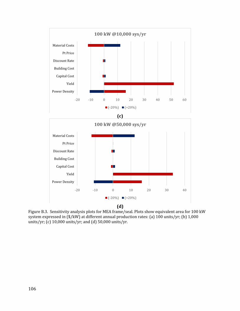
106

(c)

(d)

Figure B.3. Sensitivity analysis plots for MEA frame/seal. Plots show equivalent area for 100 kW system expressed in ($/kW) at different annual production rates: (a) 100 units/yr; (b) 1,000 units/yr; (c) 10,000 units/yr; and (d) 50,000 units/yr.

-20 -10 0 10 20 30 40 50 60

Power Density

Yield

Capital Cost

Building Cost

Discount Rate

Pt Price

Material Costs

100 kW @10,000 sys/yr

(-20%) (+20%)

-20 -10 0 10 20 30 40

Power Density

Yield

Capital Cost

Building Cost

Discount Rate

Pt Price

Material Costs

100 kW @50,000 sys/yr

(-20%) (+20%)

107

(a)

(b)

-30 -20 -10 0 10 20 30 40

Power Density

Yield

Capital Cost

Building Cost

Discount Rate

Material Costs

100 kW @100 sys/yr

Plates (-20%) Plates (+20%)

-40 -30 -20 -10 0 10 20 30 40 50

Power Density

Yield

Capital Cost

Building Cost

Discount Rate

Material Costs

100 kW @1,000 sys/yr

Plates (-20%) Plates (+20%)

108

(c)

(d)

Figure B.4. Sensitivity analysis plots for plates. Plots show equivalent area for 100 kW system expressed in ($/kW) at different annual production rates: (a) 100 units/yr; (b) 1,000 units/yr; (c)

10,000 units/yr; and (d) 50,000 units/yr.

-30 -20 -10 0 10 20 30 40 50

Power Density

Yield

Capital Cost

Building Cost

Discount Rate

Material Costs

100 kW @10,000 sys/yr

Plates (-20%) Plates (+20%)

-40 -30 -20 -10 0 10 20 30 40 50

Power Density

Yield

Capital Cost

Building Cost

Discount Rate

Material Costs

100 kW @50,000 sys/yr

Plates (-20%) Plates (+20%)

109

Appendix C: Balance of Plant Cost and Total System Cost Results CHP Systems with Reformate Fuel

a) Subsystem cost breakdown of CHP system with reformate fuel (1 kWe system)

b) Subsystem cost breakdown of CHP system with reformate fuel (50 kWe system)

$-

$2,000

$4,000

$6,000

$8,000

$10,000

$12,000

100 1000 10000 50000

Cost

($/k

W)

Production Volume (Systems/year)

1kW CHP Reformate Subsystems Cost Breakdown

Misc. Subsystem

Controls Subsystem

Power Subsystem

Coolant Subsystem

Air Subsystem

Fuel Processing Subsystem

$-

$200

$400

$600

$800

$1,000

$1,200

100 1000 10000 50000

Cost

($/k

W)

Production Volume (Systems/year)

50kW CHP Reformate Subsystems Cost Breakdown

Misc. Subsystem

Controls Subsystem

Power Subsystem

Coolant Subsystem

Air Subsystem

Fuel Processing Subsystem

110

c) Subsystem cost breakdown of CHP system with reformate fuel (250 kWe system) Figure C.1. Subsystem cost breakdown of CHP system with reformate fuel for a) 1 kWe system; b) 50 kWe system; c) 250 kWe system

$-

$100

$200

$300

$400

$500

$600

$700

$800

100 1,000 10,000 50,000

Cost

($/k

W)

Production Volume (Systems/year)

250kW CHP Reformate Subsystems Cost Breakdown

Misc. Subsystem

Controls Subsystem

Power Subsystem

Coolant Subsystem

Air Subsystem

Fuel Processing Subsystem

Fuel Processing Subsystem, $2,871

Air Subsystem, $440 Coolant

Subsystem, $1,001

Power Subsystem, $2,642

Controls/Metering Subsystem, $924 Misc. Subsystem,

$1,171

1kW CHP Reformate System (for 1000 units of production)

Fuel Processing Subsystem

Air Subsystem

Coolant Subsystem

Power Subsystem

Controls/Metering Subsystem

Misc. Subsystem

111

a) Subsystem cost breakdown of CHP system with reformate fuel (1 kWe system)

b) Subsystem cost breakdown of CHP system with reformate fuel (10 kWe system)

c) Subsystem cost breakdown of CHP system with reformate fuel (50 kWe system)

Fuel Processing Subsystem, $5,295

Air Subsystem, $950 Coolant

Subsystem, $1,769

Power Subsystem, $4,223

Controls/Metering Subsystem, $1,708

Misc. Subsystem, $2,616

10kW CHP Reformate System (for 1000 units of production)

Fuel Processing Subsystem

Air Subsystem

Coolant Subsystem

Power Subsystem

Controls/Metering Subsystem

Misc. Subsystem

Fuel Processing Subsystem, $11,133

Air Subsystem, $1,852

Coolant Subsystem, $4,407

Power Subsystem, $19,197

Controls/Metering Subsystem,

$5,971

Misc. Subsystem, $4,142

50kW CHP Reformate System (for 1000 units of production)

Fuel Processing Subsystem

Air Subsystem

Coolant Subsystem

Power Subsystem

Controls/Metering Subsystem

Misc. Subsystem

112

d) Subsystem cost breakdown of CHP system with reformate fuel (100 kWe system)

e) Subsystem cost breakdown of CHP system with reformate fuel (250 kWe system)

Fuel Processing Subsystem, $20,328

Air Subsystem, $3,330

Coolant Subsystem,

$9,208

Power Subsystem, $24,455

Controls/Metering Subsystem, $9,935

Misc. Subsystem, $6,097

100kW CHP Reformate System (for 1000 units of production)

Fuel Processing Subsystem

Air Subsystem

Coolant Subsystem

Power Subsystem

Controls/Metering Subsystem

Misc. Subsystem

Fuel Processing Subsystem, $20,328

Air Subsystem, $3,330

Coolant Subsystem,

$9,208

Power Subsystem, $24,455

Controls/Metering Subsystem,

$9,935

Misc. Subsystem, $6,097

100kW CHP Reformate System (for 1000 units of production)

Fuel Processing Subsystem

Air Subsystem

Coolant Subsystem

Power Subsystem

Controls/Metering Subsystem

Misc. Subsystem

113

Figure C.2. Subsystem cost breakdown of CHP system with reformate fuel for: a) 1 kWe system; b)10 kWe system; c) 50 kWe system; d) 100 kWe system; e) 250 kWe system

Subsystem/System Size 1kW 10kW 50kW 100kW 250kW Fuel Processing 32% 32% 24% 28% 28%

Air 5% 6% 4% 5% 4% Coolant 11% 11% 9% 13% 10% Power 29% 25% 41% 33% 40%

Controls 10% 10% 13% 14% 12% Miscellaneous 5% 7% 9% 12% 10%

Table C.1. Subsystem percentage cost breakdown for CHP system with reformate fuel (for 1000 systems/year)

1kW

10kW

$-

$5,000

$10,000

$15,000

$20,000

$25,000

$30,000

100 1,000 10,000 50,000

Cost

/kW

(201

3 $)

Production Volume (Systems/year)

Fuel Processor

BOP

Material Scrap ($/kWnet)

Process: Building ($/kWnet)

Process: Operational ($/kWnet)Process: Capital ($/kWnet)

Labor ($/kWnet)

Direct Material ($/kWnet)

Stack

$0

$500

$1,000

$1,500

$2,000

$2,500

$3,000

$3,500

$4,000

$4,500

$5,000

100 1,000 10,000 50,000

Cost

/kW

(201

3 $)

Production Volume (Systems/year)

Fuel Processor

BOP

Material Scrap ($/kWnet)

Process: Building ($/kWnet)

Process: Operational ($/kWnet)Process: Capital ($/kWnet)

Labor ($/kWnet)

Direct Material ($/kWnet)

Stack

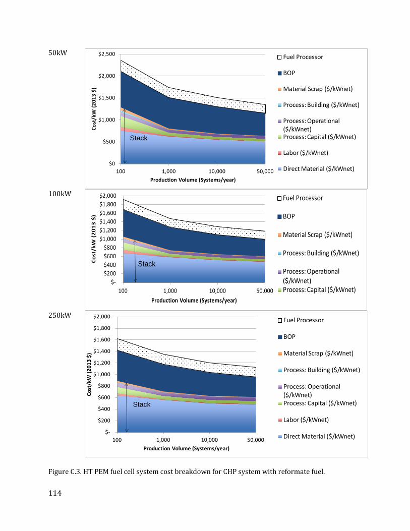
114

50kW

100kW

250kW

Figure C.3. HT PEM fuel cell system cost breakdown for CHP system with reformate fuel.

$0

$500

$1,000

$1,500

$2,000

$2,500

100 1,000 10,000 50,000

Cost

/kW

(201

3 $)

Production Volume (Systems/year)

Fuel Processor

BOP

Material Scrap ($/kWnet)

Process: Building ($/kWnet)

Process: Operational ($/kWnet)Process: Capital ($/kWnet)

Labor ($/kWnet)

Direct Material ($/kWnet)

Stack

$-$200 $400 $600 $800

$1,000 $1,200 $1,400 $1,600 $1,800 $2,000

100 1,000 10,000 50,000

Cost

/kW

(20

13 $

)

Production Volume (Systems/year)

Fuel Processor

BOP

Material Scrap ($/kWnet)

Process: Building ($/kWnet)

Process: Operational ($/kWnet)Process: Capital ($/kWnet)

Stack

$-

$200

$400

$600

$800

$1,000

$1,200

$1,400

$1,600

$1,800

$2,000

100 1,000 10,000 50,000

Cost

/kW

(201

3 $)

Production Volume (Systems/year)

Fuel Processor

BOP

Material Scrap ($/kWnet)

Process: Building ($/kWnet)

Process: Operational ($/kWnet)Process: Capital ($/kWnet)

Labor ($/kWnet)

Direct Material ($/kWnet)

Stack

115

Stack Size (kW) 1

Production Volume (Units/yr) 100 1,000 10,000 50,000

Fuel Cell Stack Direct Material ($/kWenet) 4,129.75 1,222.69 827.68 740.17

Fuel Cell Stack Labor ($/kWenet) 1,015.05 237.34 132.97 23.78 Fuel Cell Stack Process: Capital

($/kWenet) 6,045.39 806.24 166.24 80.32

Fuel Cell Stack Process: Operational ($/kWenet) 640.67 132.93 73.71 64.33

Fuel Cell Stack Process: Building ($/kWenet) 1,842.83 193.13 26.69 5.79

Fuel Cell Stack Material Scrap ($/kWenet) 2,428.17 250.93 48.66 22.94

Fuel Cell Stack Cost 16,101.86 2,843.26 1,275.95 937.32 BOP_Non-Fuel Processor 7,333.02 6,177.58 5,236.77 4,502.75

BOP_Fuel Processor 3,730.32 2,871.44 2,437.60 2,241.36 Total ($/kWnet) 27,165 11,892 8,950 7,681 Stack Size (kW) 10

Production Volume (Units/yr) 100 1,000 10,000 50,000

Fuel Cell Stack Direct Material (/kWenet) 1,077.69 708.85 606.53 558.85

Fuel Cell Stack Labor (/kWenet) 166.25 82.28 13.12 8.97 Fuel Cell Stack Process: Capital

(/kWenet) 806.24 172.57 66.65 55.71

Fuel Cell Stack Process: Operational (/kWenet) 134.17 74.59 64.10 63.21

Fuel Cell Stack Process: Building (/kWenet) 193.13 20.69 2.51 1.66

Fuel Cell Stack Material Scrap (/kWenet) 251.21 48.76 18.58 12.33

Fuel Cell Stack Cost 2,628.71 1,107.74 771.48 700.72 BOP_Non-Fuel Processor 1,336.15 1,126.70 958.42 806.50

BOP_Fuel Processor 638.40 529.50 464.12 434.51 Total (/kWnet) 4,603 2,764 2,194 1,942

Stack Size (kW) 50

Production Volume (Units/yr) 100 1,000 10,000 50,000

116

Fuel Cell Stack Direct Material ($/kWenet) 749.74 618.37 547.70 505.39

Fuel Cell Stack Labor ($/kWenet) 88.93 16.51 8.34 7.44 Fuel Cell Stack Process: Capital

($/kWenet) 255.71 77.19 55.40 53.66

Fuel Cell Stack Process: Operational ($/kWenet) 82.25 65.62 63.12 62.87

Fuel Cell Stack Process: Building ($/kWenet) 41.81 4.19 1.50 1.25

Fuel Cell Stack Material Scrap ($/kWenet) 71.96 22.92 12.31 7.26

Fuel Cell Stack Cost 1,290 805 688 638 BOP_Non-Fuel Processor 818 711 615 522

BOP_Fuel Processor 258 223 204 195 Total ($/kWnet) 2,367 1,739 1,507 1,356

Stack Size (kW) 100

Production Volume (Units/yr) 100 1,000 10,000 50,000 Fuel Cell Stack Direct Material

($/kWenet) 675.75 578.07 514.17 474.74

Fuel Cell Stack Labor ($/kWenet) 76.38 12.09 7.51 7.05 Fuel Cell Stack Process: Capital

($/kWenet) 172.58 66.65 54.43 51.63

Fuel Cell Stack Process: Operational ($/kWenet) 72.90 62.50 61.36 61.19

Fuel Cell Stack Process: Building ($/kWenet) 13.22 3.04 1.29 1.16

Fuel Cell Stack Material Scrap ($/kWenet) 48.05 18.17 9.87 5.29

Fuel Cell Stack Cost 1,058.87 740.52 648.64 601.06 BOP_Non-Fuel Processor 622.55 530.25 452.54 397.48

BOP_Fuel Processor 230.56 203.28 189.20 182.16 Total ($/kWnet) 1,912 1,474 1,290 1,181

Stack Size (kW) 250

Production Volume (Units/yr) 100 1,000 10,000 50,000

Fuel Cell Stack Direct Material ($/kWenet) 635.14 557.12

497.03 481.81

Fuel Cell Stack Labor ($/kWenet) 35.55 8.52 7.21 6.98

117

Fuel Cell Stack Process: Capital ($/kWenet) 113.21 60.57

53.53 52.20

Fuel Cell Stack Process: Operational ($/kWenet) 68.48 62.70

62.06 62.09

Fuel Cell Stack Process: Building ($/kWenet) 6.05 1.75

1.21 1.15

Fuel Cell Stack Material Scrap ($/kWenet) 30.49 14.54

7.21 5.48

Fuel Cell Stack Cost 888.93 705.21 628.25 609.72

BOP_Non-Fuel Processor 531.99 466.11 402.88 345.23

BOP_Fuel Processor 198.00 178.64 170.72 165.44

Total ($/kWnet) 1,619 1,350 1,202 1,120

Table C.2: Cost breakdown for HT PEM system with reformate fuel 1kW

0%

10%

20%

30%

40%

50%

60%

70%

80%

90%

100%

100 1,000 10,000 50,000Production Volume (Systems/year)

BOP_FuelProcessorBOP_Non-FP

Stack Cost

118

10kW

50kW

0%10%20%30%40%50%60%70%80%90%

100%

100 1,000 10,000 50,000Production volume (Systems/year)

BOP_FuelProcessorBOP_Non-FP

Stack Cost

0%

10%

20%

30%

40%

50%

60%

70%

80%

90%

100%

100 1,000 10,000 50,000Production Volume (Systems/year)

BOP_FuelProcessor

BOP_Non-FP

Stack Cost

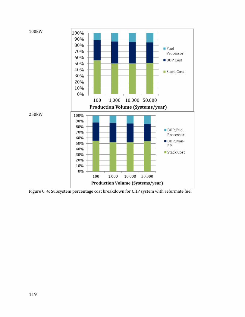
119

100kW

250kW

Figure C. 4: Subsystem percentage cost breakdown for CHP system with reformate fuel

0%10%20%30%40%50%60%70%80%90%

100%

100 1,000 10,000 50,000Production Volume (Systems/year)

FuelProcessor

BOP Cost

Stack Cost

0%10%20%30%40%50%60%70%80%90%

100%

100 1,000 10,000 50,000

Production Volume (Systems/year)

BOP_FuelProcessorBOP_Non-FPStack Cost

120

1kW

10kW

0%10%20%30%40%50%60%70%80%90%

100%

100 1000 10000 50000Production Volume (Systems/year)

Stack Cost Breakdown (1 kW FC System)

Assembly

Plates

Frame/Sealing

GDE

Membrane

0%10%20%30%40%50%60%70%80%90%

100%

100 1000 10000 50000Production Volume (Systems/year)

Stack Cost Breakdown (10 kW FC System)

Assembly

Plates

Frame/Sealing

GDE

Membrane

121

50kW

100kW

0%10%20%30%40%50%60%70%80%90%

100%

100 1000 10000 50000Production Volume (Systems/year)

Stack Cost Breakdown (50 kW FC System)

Assembly

Plates

Frame/Sealing

GDE

Membrane

0%10%20%30%40%50%60%70%80%90%

100%

100 1000 10000 50000Production Volume (Systems/year)

Stack Cost Breakdon (100 kW FC System)

Assembly

Plates

Frame/Sealing

GDE

Membrane

122

250kW

Figure C. 5: Stack cost percentage cost breakdown for CHP system with reformate fuel 1kW

0%10%20%30%40%50%60%70%80%90%

100%

100 1000 10000 50000Production Volume (Systems/year)

Stack Cost Breakdown (250 kW FC System)

Assembly

Plates

Frame/Sealing

GDE

Membrane

0

10000

20000

30000

40000

50000

60000

100 1000 10000 50000

$/kW

Annual Production Volume (Systems/year)

33% Installation and Other Fees

50% Corporate Markup

BOP and FP

Stack

123

10kW

50kW

0

1000

2000

3000

4000

5000

6000

7000

8000

9000

10000

100 1000 10000 50000

$/kW

Annual Production Volume (Systems/year)

33% Installation and Other Fees

50% Corporate Markup

BOP and FP

Stack

0

500

1000

1500

2000

2500

3000

3500

4000

4500

5000

100 1000 10000 50000

$/kW

Annual Production Volume (Systems/year)

33% Installation and OtherFees50% Corporate Markup

BOP and FP

124

100kW

250kW

Figure C.6: Installed costs of the CHP HT PEMFC system

0

500

1000

1500

2000

2500

3000

3500

4000

4500

100 1000 10000 50000

$/kW

Annual Production Volume (Systems/year)

33% Installation and Other Fees

50% Corporate Markup

BOP and FP

Stack

0

500

1000

1500

2000

2500

3000

3500

4000

100 1000 10000 50000

$/kW

Annual Production Volume (Systems/year)

33% Installation and Other Fees50% Corporate MarkupBOP and FPStack

125

Appendix D: Total Cost of Ownership Modeling of CHP Fuel Cell Systems Although LT PEM report contains all assumption of the total cost of ownership modeling and its results for small hotel and large hospital, we include here significant changes between LT PEM and HT PEM fuel cells. Some of the important differences between these two PEM technologies are: equipment cost, refurbishment and replacement cost, system efficiencies (electrical and thermal). Following section discusses the method of estimating O&M cost for HT PEM fuel cell system. Estimation of Replacement Cost Example below summarizes simple calculation method to estimate Operation and Maintenance (O&M) cost for 50 kW FC system. This example is a simple economic calculation method used to estimate O&M cost. Starting with initial cost for some major subsystems and their replacement frequencies, we converted all future values to present values (NPV) using 5% discount rate, then we converted these NPVs into equal annual payments as shown below.

Part Replacement Frequency

(Year)

Capital Cost ($)*

Net Present Value (NPV)‡‡

Annual Payment ($)

Stack† 20,000 hr $37,240 $90,602.63 ($9,947.68) Reformer 5 12,651 $17,325.43 ($1,902.24) Compressor/blower 10 3,823 $2,300.05 ($252.53) Water Management sub-system

10 3,655 $2,198.98 ($241.44) Battery/startup system

5 510

$698.44 ($76.68) Total $113,125.53 ($12,420.57)

* Cost based on DFMA results for 50kW systems. *** All future values were converted to present values (2013$) using 5% discount rate † Stack is refurbished every 20,000 hours by conditioning some components like plates and putting them again in the stack (refurbishment cost=50% of the original cost), and replaced completely every 40,000 ‡ Assumed 96% availability of the system for scheduled stack replacement. ‡‡ End-of-life parts assumed to be sold at 2% of original value. Table D.1. Replacement schedule with associated cost Now for a full duty cycle, the maximum FC capacity equals to 24hr/day X 365day/yr X 50 kWX 0.96 (availability)= 420,480 kWh per year

• Displaced Electricity by FC for small hotel in Phoenix, AZ=382,253 kWh • Displaced Electricity by FC for small hotel in Minneapolis, MN=345,368 • Displaced Electricity by FC for small hotel in Chicago, IL=345,791 • Displaced Electricity by FC for small hotel in New York City, NY=314,930 • Displaced Electricity by FC for small hotel in Houston, TX=362,313

Then if we estimate average displaced power by fuel cell to be 350,000 kWh, this will give us the following O&M cost: 12,420/350k= 3.5₵ per kWh.

126

Use-phase Model and results In this section we will discuss results of the use phase model with larger fuel cell sizes: 50kWe fuel cell system for small hotel and 1MW (4X250kWe) fuel cell system for hospital. Table D.2 summarizes assumptions for 50kWe fuel cell system in small hotel.

Parameter Phoenix, AZ

Minneapolis, MN

Chicago, IL

NYC, NY Houston, TX

Unit

Building Type Small Hotel FC system size 50 kW Capital costs of FC including installation cost

3,400

$/kW

Electricity price Variable by time

Variable by time

Variable by time

Variable by time

Variable by time

$/kWh

Demand Charge 4.05 3.30 5.69 17.95 12.39 15.13 (June-Sep)

$ * Peak kWh

NG cost 0.0357 0.0258 0.0292 0.0332 0.0263 $/kWh Scheduled maintenance cost ‡

1,000 1,000 1,000 1,000 1,000 $/yr

O&M cost 0.035 0.035 0.035 0.035 0.035 $/kWh Days per year 365 365 365 365 365 day FC system availability‡‡

96% 96% 96% 96% 96%

Lifetime of system

15 15 15 15 15 yr

Interest rate 5% 5% 5% 5% 5% ‡ From CETEEM model (Lipman et al., 2004). ‡‡ In this analysis the CHP system was assumed to have a 96% availability factor and three outages during the year. One outage is assumed to be a planned maintenance outage and two are assumed to be unplanned forced outages. Table. D.2. Assumptions for cost and environmental impact model for 50 kW HT PEM fuel cell system used as a CHP system in small hotel. For the hospital case, four 250kW FC systems are included to accommodate the total demand rather than a single 1000 kW system since a 250kW system was modeled in the current analysis (Table D.3). In the use-phase model for hospitals, a new FC system is triggered if the first one is not enough to supply required electrical load (i.e. total of electricity and cooling loads) and so on for the third and fourth FC system. However, all triggered system should run at 50% or more of their rated power capacity in order to have them operating at high efficiency. (Note: the power efficiency for each individual fuel cell will fall below 30% if it is operating at <10% of its rated power). If all four systems combined together cannot supply the required load at any given time, then this unmet demand will be purchased from the grid. Similar logic was also used for total heating demand and supply; i.e. if the FC system cannot provide all of the heat demand, the system will cover these heating loads using NG-fired boiler systems. Parameter Phoenix,

AZ Minneapolis, MN

Chicago, IL

NYC, NY Houston, TX

San Diego, CA

Unit

Building Type Hospital FC system size 250X4 kW Capital costs of FC including installation cost

3,000

$/kW

127

Electricity price Variable by time

Variable by time

Variable by time

Variable by time

Variable by time

$/kWh

Demand Charge 4.05 8.98 12.86 (June-

Sep)

5.86 17.95 12.39 15.13 (June-Sep)

19.96 $ * Peak kWh

NG cost 0.0357 0.0258 0.0292 0.0332 0.0263 0.0277 $/kWh Scheduled maintenance cost ‡

3,000 3,000 3,000 3,000 3,000 $/yr

O&M cost 0.035 0.035 0.035 0.035 0.035 $/kWh Days per year 365 365 365 365 365 day FC system availability‡‡

96% 96% 96% 96% 96%

Lifetime of system 15 15 15 15 15 yr Interest rate 5% 5% 5% 5% 5% From CETEEM model (Lipman et al., 2004). ‡‡ In this analysis the CHP system was assumed to have a 96% availability factor and three outages during the year. One outage is assumed to be a planned maintenance outage and two are assumed to be unplanned forced outages. Table. D.3. Life cycle cost analysis assumptions for hospital case (1MW FC system). Use phase results for small hotel and large hospital are shown in Tables D.4 and D.5, respectively.

128

Table D.4. Output results from use-phase model for small (50kW FC system).

OutputNo Fuel

CellFuel Cell

No Fuel Cell

Fuel CellNo Fuel

CellFuel Cell

No Fuel Cell

Fuel CellNo Fuel

CellFuel Cell

FC System Utilization 82.30% 78.90% 79% 71.90% 82.70%

FC Heat Utilization WH+SH

13.00% 39.10% 33% 32.60% 10.80%

Total Electricity Demand (kWh/yr) Total Space Heating Demand (kWh/yr) Total Water Heating Demand (kWh/yr) Annual Generated Power by FC (kWh) 382,253

345,368 345,791 314,930 362,313

Annual Generated Heat by FC (kWh) 671,725 595,698 596,811 539,856 632,809

Capital Cost 0 1.64E+04 0 1.64E+04 0 1.64E+04 0 1.64E+04 0 1.64E+04O&M Cost 0 13,379 0 1.21E+04 0 1.21E+04 0 1.10E+04 0 1.27E+04Scheduled Maintenance 0 1000 0 1000 0 1000 0 1000 0 1000Fuel Cost- FCS only 0 4.70E+04 0 3.04E+04 0 3.45E+04 0 3.55E+04 0 3.28E+04Residual Fuel 3574.3 0 7778.815 18.270415 7448.98 0.294638 8351.96 0.284427 2184.77 0Electrcity Cost 4.73E+04 1.54E+04 4.54E+04 6679.1689 3.21E+04 4888.965 8797.94 990.2948 1.54E+04 3727.641Dmenad Charge 5444.82 3635.28 3421.77 1936.77 6020.59 3460.089 1.70E+04 8881.66 1.55E+04 9422.297Fixed Monthly Charge 149.64 149.64 131.16 131.16 347.88 347.88 1240.56 1240.56 295.44 295.44Cost ($/yr) FC supplies both space heating and Hot water

56,473 96,941 56,706 68,586 45,922 72,665 35,350 74,979 33,397 76,267

GHG (ton CO2/yr) FC supplies both space heating and Hot water

298 338.483 404.695 263.695 338.787 237.787 147.998 151.998 277.300 299.300

Capital Cost 0 1.64E+04 0 1.64E+04 0 1.64E+04 0 1.64E+04 0 1.64E+04O&M Cost 0 13,379 0 1.21E+04 0 1.21E+04 0 1.10E+04 0 1.27E+04Scheduled Maintenance 0 1000 0 1000 0 1000 0 1000 0 1000Fuel Cost- FCS only 0 4.70E+04 0 3.04E+04 0 3.45E+04 0 3.55E+04 0 3.28E+04Residual Fuel 3574.3 830.9055 7778.815 4503.1263 7448.98 3971.451 8351.96 4504.0579 2184.77 0Electrcity Cost 4.73E+04 1.54E+04 4.54E+04 6679.1689 3.21E+04 4888.965 8797.94 990.2948 1.54E+04 3727.641Dmenad Charge 5444.82 3635.28 3421.77 1936.77 6020.59 3460.089 1.70E+04 8881.66 1.55E+04 9422.297Fixed Monthly Charge 149.64 149.64 131.16 131.16 347.88 347.88 1240.56 1240.56 295.44 295.44Cost ($/yr) FC supplies Hot water only

56,473 97,772 56,706 73,071 45,922 76,636 35,350 79,483 33,397 76,267

GHG (ton CO2/yr) FC supplies Hot water only

298 343.983 404.695 308.795 338.787 276.687 147.998 170.598 277.300 303.400

FC supplies hot water only

FC supplies space and water heating

576,668

23,307

76,954 118,971 116,075

419,590

83,071

424,147 369,661 497,656

135,869 135,869 0174,743

127,112

129

Table D.5. Output results from use-phase model for hospital (1MW FC system). Tables D.6 and D.7 summarize LCIA results for small hotel case using 50kWe fuel cell system in which waste heat is utilized for water heating only (Table D.6) and space and water heatings (Table D.7). Similarly Tables D.8 and D.9 summarizes LCIA results for 1MW fuel cell system used in the hospital case. Table D.8 summarizes LCIA results when waste heat is used for water heating only,

OutputNo Fuel

CellFuel Cell

No Fuel Cell

Fuel CellNo Fuel

CellFuel Cell

No Fuel Cell

Fuel CellNo Fuel

CellFuel Cell

No Fuel Cell

Fuel Cell

FC System Utilization 96.50% 79.70% 85% 83.10% 98.11% 24.70%

FC Heat Utilization WH+SH

18.00% 24.50% 23% 27.40% 18.80% 3.84%

Total Electricity Demand (MWh/yr) Total Space Heating Demand (MWh/yr) Total Water Heating Demand (MWh/yr) Annual Generated Power by FC (MWh) 8,112

6,703 7,117 6,989 8,251 2,080

Annual Generated Heat by FC (MWh) 1.42E+07 1.23E+07 1.29E+07 12,804,450 1.42E+07 5.27E+06

Capital Cost 0 3.61E+05 0 3.61E+05 0 3.61E+05 0 3.61E+05 0 3.61E+05 0 3.61E+05O&M Cost 0 2.84E+05 0 2.35E+05 0 2.49E+05 0 2.45E+05 0 2.89E+05 0 7.28E+04Scheduled Maintenance 0 3.00E+03 0 3000 0 3000 0 3000 0 3000 0 3000Fuel Cost- FCS only 0 972,278 0 575,782 0 694,942 0 772,848 0 731,395 0 185,096Residual Fuel Cost 1.01E+05 0.00E+00 9.95E+04 394.81358 1.08E+05 46.90441 1.43E+05 1733.256 7.79E+04 0 1.68E+04 0Electrcity Cost 6.29E+05 4.91E+04 4.49E+05 2.14E+04 5.94E+05 3.34E+04 1.81E+05 8176.4186 2.96E+05 2.91E+04 1.86E+05 0Dmenad Charge 6.38E+04 2.53E+04 1.48E+05 4.83E+04 8.75E+04 3.15E+04 2.61E+05 8.94E+04 2.16E+05 8.71E+04 6.75E+04 1.50E+04Fixed Monthly Charge 6366.96 6366.96 340.56 340.56 516 516 1240.56 1240.56 295.44 295.44 2794.44 2794.44Cost ($/yr) FC supplies both space heating and Hot water

800,020 1,701,225 697,198 1,245,051 789,276 1,373,772 586,142 1,482,282 589,224 1,500,913 273,381 639,972

GHG (ton CO2/yr) FC supplies space and water heating

4,956 5,680 6,815 4,963 6,084 4,319 2,892 3,141 5,560 5,996 1,162 1,371

Capital Cost 0 3.61E+05 0 3.61E+05 0 3.61E+05 0 3.61E+05 0 3.61E+05 0 3.61E+05O&M Cost 0 2.84E+05 0 2.35E+05 0 2.49E+05 0 2.45E+05 0 2.89E+05 0 7.28E+04Scheduled Maintenance 0 3.00E+03 0 3000 0 3000 0 3000 0 3000 0 3000Fuel Cost- FCS only 0 972,278 0 575,782 0 694,942 0 772,848 0 731,395 0 185,096Residual Fuel Cost 1.01E+05 9.59E+04 9.95E+04 93617.215 1.08E+05 101331.9 1.43E+05 135979.72 7.79E+04 73944.23 1.68E+04 14664.8Electrcity Cost 6.29E+05 4.91E+04 4.49E+05 2.14E+04 5.94E+05 3.34E+04 1.81E+05 8176.4186 2.96E+05 2.91E+04 1.86E+05 0Dmenad Charge 6.38E+04 2.53E+04 1.48E+05 4.83E+04 8.75E+04 3.15E+04 2.61E+05 8.94E+04 2.16E+05 8.71E+04 6.75E+04 1.50E+04Fixed Monthly Charge 6366.96 6366.96 340.56 340.56 516 516 1240.56 1240.56 295.44 295.44 2794.44 2794.44Cost ($/yr) FC supplies both space heating and Hot water

800,020 1,797,087 697,198 1,338,273 789,276 1,475,057 586,142 1,616,529 589,224 1,574,857 273,381 654,637

GHG (ton CO2/yr) FC supplies Hot water only

4,956 6,265 6,815 5,551 6,084 5,447 2,892 3,983 5,560 6,556 1,162 1,489

FC supplies space and water heating

FC supplies hot water only

2,689

140 151 76

Chicago, IL

3,633

230

Minneapolis, MN

7,331

3,467 4,102 2,812 529

215 210

7,852 7,624 9,533 2,166

Phoenix, AZ

9,140

NYC, NY Houston, TX San Diego, CA

130

while Table D.9 summarizes LCIA results when fuel cell system is used for space and water heatings. Table D.6. LCIA results for 50kWe fuel cell system used in the small hotel. Waste heat is utilized for water heating application only.

Table D.7. LCIA results for 50kWe fuel cell system used in the small hotel. Waste heat is utilized for space and water heating.

Table D.8. LCIA results for 1MWe fuel cell system used in the hospital. Waste heat is utilized for water heating application only.

Output Phoenix Minneapolis ChicagoNew York

City Houston

Annual Generated Power by FC (kWh) 382,253 345,368 345,791 314,930 362,313Annual Generated Heat by FC (kWh) 671,725 595,698 596,811 539,856 632,809Avoided GHG [tCO2e/y] -45.5 95.9 62.1 -22.6 -26.1Avoided NOx [tNOx/y] 0.137 0.413 0.363 0.123 0.130Avoided SOx [tSOx/y] 0.086 0.786 1.232 0.202 0.151Avoided PM10 [t/y] 0.0015 0.0012 0.0014 0.0015 0.00071Avoided PM2.5 [t/y] 0.00045 0.00022 0.00025 0.00039 0.0000GHG credit at $44/ton CO2 ($/kWhe) -0.0052 0.012 0.008 -0.003 -0.0032

Health, Environmental Savings ($/kWhe) 0.0013 0.018 0.027 0.007 0.0018

Output Phoenix Minneapolis ChicagoNew York

City Houston

Annual Generated Power by FC (kWh) 382,253 345,368 345,791 314,930 362,313Annual Generated Heat by FC (kWh) 671,725 595,698 596,811 539,856 632,809Avoided GHG [tCO2e/y] -40 141 101 -4 -22Avoided NOx [tNOx/y] 0.142 0.464 0.406 0.137 0.133Avoided SOx [tSOx/y] 0.092 0.865 1.339 0.236 0.152Avoided PM10 [t/y] 0.0019 0.0028 0.0029 0.0023 0.00088Avoided PM2.5 [t/y] 0.00059 0.00053 0.00053 0.00084 0.0000GHG credit at $44/ton CO2 ($/kWhe) -0.0046 0.018 0.013 -0.001 -0.0026

Health, Environmental Savings ($/kWhe) 0.0015 0.020 0.030 0.010 0.0019

Output Phoenix Minneapolis ChicagoNew York

City Houston San Diego

Annual Generated Power by FC (MWh) 8,112 6,703 7,117 6,989 8,251 2080Annual Generated Heat by FC (MWh) 14,154 12,345 12,913 12,804 14,177 5272Avoided GHG [tCO2e/y] -1309 1264 637 -1091 -996 -327Avoided NOx [tNOx/y] 2.62 7.34 6.77 2.27 2.67 0.68Avoided SOx [tSOx/y] 1.47 14.16 23.60 3.89 3.30 0.38Avoided PM10 [t/y] 0.0022 0.0033 0.0020 0.0033 0.0021 0.00063Avoided PM2.5 [t/y] 0.00023 0.00061 0.00010 0.00088 0.00011 0.00006GHG credit at $44/ton CO2 ($/kWhe) -0.0071 0.0083 0.0039 -0.0069 -0.005 -0.0069

Health, Environmental Savings ($/kWhe) 0.0009 0.0158 0.0251 0.0044 0.002 0.0014

131

Table D.9. LCIA results for 1MWe fuel cell system used in the hospital. Waste heat is utilized for space and water heating.

Total Cost of Ownership Model Results Tables D.10 and D.11 show TCO results for 50kW FC system in small hotel case and 1MW FC system in large hospital case, respectively. A water fall plot was made for the 50kW fuel cell system used in small hotel in Chicago, IL and shows that space and water heating can offset 13.3% of the levelized cost of electricity (Figure D.1). GHG credits provide 10.4% savings at $44 per ton of CO2-eq, and health and environmental savings provide 11.6% savings. Total savings from heating and externalities is about 35% for the case of CHP with offset water heating and space heating.

Output Phoenix Minneapolis ChicagoNew York

City Houston San Diego

Annual Generated Power by FC (MWh) 8,112 6,703 7,117 6,989 8,251 2080Annual Generated Heat by FC (MWh) 14,154 12,345 12,913 12,804 14,177 5272Avoided GHG [tCO2e/y] -724 1852 1765 -249 -436 -209Avoided NOx [tNOx/y] 3.11 7.85 8.01 2.98 3.14 0.77Avoided SOx [tSOx/y] 1.63 14.50 26.65 4.74 3.38 0.42Avoided PM10 [t/y] 0.0445 0.0550 0.0340 0.0678 0.0407 0.00502Avoided PM2.5 [t/y] 0.00469 0.01028 0.00176 0.01811 0.00210 0.00050GHG credit at $44/ton CO2 ($/kWhe) -0.0039 0.0122 0.0109 -0.0016 -0.0023 -0.0044

Health, Environmental Savings ($/kWhe) 0.0013 0.0179 0.0286 0.0101 0.002 0.0020

132

Table D.10. TCO results for 50kW kW FC system used in small hotel (water and space heating)

No FCS Fuel Cell No FCS Fuel Cell No FCS Fuel Cell No FCS Fuel Cell No FCS Fuel CellFC System Utilization 82.3% 78.9% 79.0% 71.9% 82.7%Total Electricity Demand (kWh/yr)

576,668 576,668 419,590 419,590 424,147 424,147 369,661 369,661 497,656 497,656

Total Space Heating Demand (kWh/yr) Total Water Heating Demand (kWh/yr) Annual Generated Power by FC (kWh)

382,253 345,368 345,791 314,930 362,313

FC fraction of Electricity Demand 66% 82% 82% 85% 73%Annual Generated Heat by FC (kWh)

671,725 595,698 596,811 539,856 632,809

Capital Cost ($/yr) 16,400 16,400 16,400 16,400 16,400O&M Cost ($/yr) 13,379 12,100 12,100 11,000 12,700Scheduled Maintenance ($/yr) 1,000 1,000

1,000 1,000 1,000

Fuel Cost for Fuel Cell ($/yr) 47,000 30,400 34,500 35,500 32,800Fuel Cost for Conv. Heating ($/yr)

3574 0 7779 18 7449 0 8352 0 2185 0

Purchased Electricity Energy Cost ($/yr) 47305 15360 45374 6679 32104 4889 8798 9.90E+02 15427 3728Demand Charge ($/yr) 5445 3635 3422 1937 6021 3460 16959 8882 15490 9422Fixed Charge, Electricity ($/yr) 150 150 131 131 348 348 1241 1241 295 295Total Electricity Cost ($/yr) 5.29E+04 96924 4.89E+04 68647 3.85E+04 72697 2.70E+04 75013 3.12E+04 7.63E+04Total Cost of Electricity ($/kWh)

0.092 0.168 0.117 0.164 0.091 0.171 0.073 0.203 0.063 0.153

Purchased Electricity Cost ($/kWh)

0.092 0.098 0.117 0.118 0.091 0.111 0.073 0.203 0.063 0.099

LCOE of FC power ($/kWh) 0.203 0.173 0.185 0.203 0.174Fuel savings from conventional heating ($/yr)

3574 7761 7449 8352 2185

Fuel savings per kWh($/kWh)0.009 0.022 0.022 0.027 0.006

LCOE of FC power with fuel savings ($/kWh)

0.194 0.151 0.164 0.176 0.168

GHG credit at $44/ton CO2

($/kWh)-0.0046 0.0180 0.0129 -0.0006 -0.0026

Health, Environmental Savings ($/kWh)

0.0015 0.0204 0.0301 0.0104 0.0019

LCOE with TCO Savings for Fuel Cell Power ($/kWh)

0.197 0.113 0.121 0.167 0.168

LCOE with TCO Savings for FC and Purchased Power, ($/kWh)

0.164 0.114 0.119 0.172 0.150

Output Phoenix, AZ Minneapolis, MN Chicago, IL NYC, NY Houston, TX

23,307 174,743 135,869 135,869 0

76,954 127,112 118,971 116,075 83,071

133

Table D.11. TCO results for 1MW kW FC system used in small hotel (water and space heating)

No FCS Fuel Cell No FCS Fuel Cell No FCS Fuel Cell No FCS Fuel Cell No FCS Fuel Cell No FCS Fuel CellFC System Utilization 96.5% 79.7% 84.6% 83.1% 98.1% 0.247Total Electricity Demand (MWh/yr)

9,140 9,140 7,331 7,331 7,852 7,852 7,624 7,624 9,533 9,533 2166.4 2166.4

Total Space Heating Demand (MWh/yr) Total Water Heating Demand (MWh/yr) Annual Generated Power by FC (MWh)

8,112 6,703 7,117 6,989 8,251 2080

FC fraction of Electricity Demand

89% 91% 91% 92% 87% 96%

Annual Generated Heat by FC (MWh)

14,200 12,300 12,900 12,804 14,200 5270

Capital Cost ($/yr) 361,000 361,000 361,000 361,000 361,000 361000O&M Cost ($/yr) 284,000 235,000 249,000 245,000 289,000 72800Scheduled Maintenance ($/yr)

3,000 3,000 3,000 3,000 3,000 3000

Fuel Cost for Fuel Cell ($/yr) 972,278 575,782 694,942 772,848 731,395 185096Fuel Cost for Conv. Heating ($/yr)

101000 0 99500 395 108000 47 143000 1,733 77900 0 16800 0

Purchased Electricity Energy Cost ($/yr)

629000 49,100 449000 21,400 594000 33,400 181000 8,176 296000 29,100 186000 0

Demand Charge ($/yr) 63800 25,300 148000 48,300 87500 31,500 261000 89,400 216000 87,100 67500 15000Fixed Charge, Electricity ($/yr)

6367 6367 341 341 516 516 1241 1241 295 295 2794 2794

Total Electricity Cost ($/yr) 699167 1701045 597341 1244823 682016 1373358 443241 1480665 512295 1500890 256294 639690Total Cost of Electricity ($/kWh)

0.076 0.186 0.081 0.170 0.087 0.175 0.058 0.194 0.054 0.157 0.118 0.295

Purchased Electricity Cost ($/kWh)

0.076 0.079 0.081 0.112 0.087 0.089 0.058 0.156 0.054 0.091 0.118 0.205

LCOE of FC power ($/kWh) 0.200 0.175 0.184 0.198 0.168 0.299Fuel savings from conventional heating ($/yr)

101000 99105 107953 141267 77900 16800

Fuel savings per kWh ($/kWh)

0.0125 0.0148 0.0152 0.0202 0.0094 0.0081

LCOE of FC power with fuel savings ($/kWh)

0.187 0.160 0.169 0.177 0.158 0.291

GHG credit at $44/ton CO2

($/kWh)-0.0039 0.0122 0.0109 -0.0016 -0.0023 -0.0044

Health, Environmental Savings ($/kWh)

0.0013 0.0179 0.0286 0.0101 0.0022 0.0020

LCOE with TCO Savings for Fuel Cell Power ($/kWh)

0.190 0.130 0.129 0.169 0.158 0.293

LCOE with TCO Savings for FC and Purchased Power, ($/kWh)

0.177 0.129 0.125 0.168 0.149 0.290

Output Phoenix, AZ Minneapolis, MN Chicago, IL NYC, NY Houston, TX San Diego, CA

75.5

2,689 3,633 3,467 4,102 2812 528.8

140 230 215 210 151

134

Figure D.1. Levelized and total cost of electricity for a 50kW small hotel in Chicago, IL.