Generative Models for Discovering Sparse Distributed

Representations

Geo�rey E. Hinton and Zoubin Ghahramani

Department of Computer Science

University of Toronto

Toronto, Ontario, M5S 1A4, Canada

hinton@cs.toronto.edu, zoubin@cs.toronto.edu

May 9, 1997

A modi�ed version to appear in Philosophical Transactions of the Royal Society B, 1997.

Abstract

We describe a hierarchical, generative model that can be viewed as a non-linear gener-

alization of factor analysis and can be implemented in a neural network. The model uses

bottom-up, top-down and lateral connections to perform Bayesian perceptual inference cor-

rectly. Once perceptual inference has been performed the connection strengths can be updated

using a very simple learning rule that only requires locally available information. We demon-

strate that the network learns to extract sparse, distributed, hierarchical representations.

1 Introduction

Many neural network models of visual perception assume that the sensory input arrives at thebottom, visible layer of the network and is then converted by feedforward connections into suc-cessively more abstract representations in successive hidden layers. Such models are biologicallyunrealistic because they do not allow for top-down e�ects when perceiving noisy or ambiguous data(Mumford, 1994; Gregory, 1970) and they do not explain the prevalence of top-down connectionsin cortex.

In this paper, we take seriously the idea that vision is inverse graphics (Horn, 1977) and sowe start with a stochastic, generative neural network that uses top-down connections to convertan abstract representation of a scene into an intensity image. This neurally instantiated graphicsmodel is learned and the top-down connection strengths contain the network's visual knowledgeof the world. Visual perception consists of inferring the underlying state of the stochastic graphicsmodel using the false but useful assumption that the observed sensory input was generated by themodel. Since the top-down graphics model is stochastic there are usually many di�erent states ofthe hidden units that could have generated the same image, though some of these hidden statecon�gurations are typically much more probable than others. For the simplest generative models,

1

it is tractable to represent the entire posterior probability distribution over hidden con�gurationsthat results from observing an image. For more complex models, we shall have to be content witha perceptual inference process that picks one or a few con�gurations roughly according to theirposterior probabilities (Hinton and Sejnowski, 1983).

One advantage of starting with a generative model is that it provides a natural speci�cation ofwhat visual perception ought to do. For example, it speci�es exactly how top-down expectationsshould be used to disambiguate noisy data without unduly distorting reality. Another advantage isthat it provides a sensible objective function for unsupervised learning. Learning can be viewed asmaximizing the likelihood of the observed data under the generative model. This is mathematicallyequivalent to discovering e�cient ways of coding the sensory data, because the data could becommunicated to a receiver by sending the underlying states of the generative model and this isan e�cient code if and only if the generative model assigns high probability to the sensory data.

In this paper we present a sequence of progressively more sophisticated generative models.For each model, the procedures for performing perceptual inference and for learning the top-down weights follow naturally from the generative model itself. We start with two very simplemodels, factor analysis and mixtures of Gaussians, that were �rst developed by statisticians.Many of the existing models of how cortex learns are actually even simpler versions of thesestatistical approaches in which certain variances have been set to zero. We explain factor analysisand mixtures of Gaussians in some detail. To clarify the relationships between these statisticalmethods and neural network models, we describe the statistical methods as neural networks thatcan both generate data using top-down connections and perform perceptual interpretation ofobserved data using bottom-up connections. We then describe a historical sequence of moresophisticated hierarchical, non-linear generative models and the learning algorithms that go withthem. We conclude with a new model, the recti�ed Gaussian belief net, and present exampleswhere it is very e�ective at discovering hierarchical sparse distributed representations of the typeadvocated by Barlow (1989) and Olshausen and Field (1996). The new model makes strongsuggestions about the role of both top-down and lateral connections in cortex and it also suggestswhy topographic maps are so prevalent.

2 Mixtures of Gaussians

A mixture of Gaussians is a model that describes some real data points in terms of underlyingGaussian clusters. There are three aspects of this model which we shall discuss. First, givenparameters that specify the means, variances and mixing proportions of the clusters, the modelde�nes a generative distribution which assigns a probability to any possible data point. Second,given the parameter values and a data point, the perceptual interpretation process infers theposterior probability that the data came from each of the clusters. Third, given a set of observeddata points, the learning process adjusts the parameter values to maximize the probability thatthe generative model would produce the observed data.

Viewed as a neural network, a mixture of Gaussians consists of a layer of visible units whosestate vector represents a data point and a layer of hidden units each of which represents a cluster(see �gure 1). To generate a data point we �rst pick one of the hidden units, j, with a probability�j and give it a state sj = 1. All other hidden states are set to 0. The generative weight vector ofthe hidden unit, gj, represents the mean of a Gaussian cluster. When unit j is activated it sends

2

a top-down input of gji to each visible unit, i. Local, zero-mean, Gaussian noise with variance�2i is added to the top-down input to produce a sample from an axis-aligned Gaussian that hasmean gj and a covariance matrix that has the �2i terms along the diagonal and zero elsewhere.The probability of generating a particular vector of visible states, d with elements di, is therefore:

p(d) =Xj

�jYi

1p2��i

e�(di�gji)2=2�2i (1)

j

i

gji

hidden units

visible units

Figure 1: A generative neural network for mixtures of Gaussians.

Interpreting a data point, d, consists of computing the posterior probability that it was gen-erated from each of the hidden units, assuming that it must have come from one of them. Eachhidden unit, j, �rst computes the probability density of the data point under its Gaussian model:

p(djsj = 1) =Yi

1p2��i

e�(di�gji)2=2�2i (2)

These conditional probabilities are then weighted by the mixing proportions, �j, and normal-ized to give the posterior probability or responsibility of each hidden unit, j, for the data point.By Bayes theorem:

p(sj = 1jd) = �j p(djsj = 1)Pk �k p(djsk = 1)

(3)

The computation of p(djsj = 1) in Eq. 2 can be done very simply by using recognition

connections, rij, from the visible to the hidden units. The recognition connections are set equalto the generative connections, rij = gji. The normalization in Eq. 3 could be done by usingdirect lateral connections or interneurons to ensure that the total activity in the hidden layer is aconstant.

Learning consists of adjusting the generative parameters g, �, � so as to maximize the productof the probabilities assigned to all the observed data points by Eq. 1. An e�cient way to performthe learning is to sweep through all the observed data points computing p(sj = 1jd) for eachhidden unit and then to reset all the generative parameters in parallel. Angle brackets are usedto denote averages over the training data.

gj(new) = hp(sj = 1jd) di = hp(sj = 1jd)i (4)

�2i (new) =

*Xj

p(sj = 1jd) (di � gji)2

+(5)

�j(new) = hp(sj = 1jd)i (6)

3

This is a version of the \Expectation and Maximization"algorithm (Dempster et al., 1977) andis guaranteed to raise the likelihood of the observed data unless it is already at a local optimum.The computation of the posterior probabilities of the hidden states given the data (i.e. perceptualinference) is called the E-step and the updating of the parameters is called the M-step.

Instead of performing an M-step after a full sweep through the data it is possible to use anonline gradient algorithm that uses the same posterior probabilities of hidden states but updateseach generative weight using a version of the delta rule with a learning rate of �:

�gji = � p(sj = 1jd)(di � gji) (7)

The k-means algorithm (a form of vector quantization) is the limiting case of a mixture ofGaussians model where the variances are assumed equal and in�nitesimal and the �j are assumedequal. Under these assumptions the posterior probabilities in Eq. 3 go to binary values withp(sj = 1jd) = 1 for the Gaussian whose mean is closest to d and 0 otherwise. Competitivelearning algorithms (e.g. Rumelhart and Zipser, 1985) can generally be viewed as ways of �ttingmixture of Gaussians generative models. They are usually ine�cient because they do not use afull M-step and slightly wrong because they pick a single winner among the hidden units insteadof making the states proportional to the posterior probabilities.

Kohonen's self-organizing maps (Kohonen, 1982), Durbin and Willshaw's elastic net (1987),and the generative topographic map (Bishop et al., In Press) are variations of vector quantizationor mixture of Gaussian models in which additional constraints are imposed that force neighboringhidden units to have similar generative weight vectors. These constraints typically lead to a modelof the data that is worse when measured by Eq. 1. So in these models, topographic maps are nota natural consequence of trying to maximize the likelihood of the data. They are imposed onthe mixture model to make the solution easier to interpret and more brain-like. By contrast, thealgorithm we present later has to produce topographic maps to maximize the data likelihood in asparsely connected net.

Because the recognition weights are just the transpose of the generative weights and becausemany researchers do not think in terms of generative models, neural network models that performcompetitive learning typically only have the recognition weights required for perceptual inference.The weights are learned by applying the rule that is appropriate for the generative weights. Thismakes the model much simpler to implement but harder to understand.

Neural net models of unsupervised learning that are derived from mixtures have simple learn-ing rules and produce representations that are a highly non-linear function of the data, but theysu�er from a disastrous weakness in their representational abilities. Each data point is representedby the identity of the winning hidden unit (i.e. the cluster it belongs to). So for the representationto contain, on average, n bits of information about the data, there must be at least 2n hiddenunits.1

1This point is often obscured by the fact that the posterior distribution is a vector of real-valued states acrossthe hidden units. This vector contains a lot of information about the data and supervised Radial Basis Functionnetworks make use of this rich information. However, from the generative or coding viewpoint, the posteriordistribution must be viewed as a probability distribution across discrete impoverished representations, not a real-valued representation.

4

3 Factor Analysis

In factor analysis, correlations among observed variables are explained in terms of shared hiddenvariables called factors which have real-valued states. Viewed as a neural network, the generativemodel underlying a standard version of factor analysis assumes that the state, yj of each hiddenunit, j, is chosen independently from a zero-mean unit-variance Gaussian and the state, di, of eachvisible unit, i, is then chosen from a Gaussian with variance �2i and mean

Pj yjgji. So the only

di�erence from the mixture of Gaussians model is that the hidden state vectors are continuousand Gaussian distributed rather than discrete vectors that contain a single 1.

The probability of generating a particular vector of visible states, d, is obtained by integratingover all possible states, y, of the hidden units, weighting each hidden state vector by its probabilityunder the generative model.

p(d) =

Zp(y)p(djy)dy (8)

=

Z Yj

1p2�

e�y2

j=2Yi

1p2��i

e�(di�

Pjyjgji)

2=2�2i dy (9)

Because the network is linear and the noise is Gaussian, this integral is tractable.

Maximum likelihood factor analysis (Everitt, 1984) consists of �nding generative weights andlocal noise levels for the visible units so as to maximize the likelihood of generating the observeddata. Without loss of generality, the generative noise model for the hidden units can be set to bea zero mean Gaussian with a covariance equal to the identity matrix.

3.1 Computing posterior distributions

Given some generative parameters and an observed data point, the perceptual inference problemis to compute the posterior distribution in the continuous hidden space. This is not as simple ascomputing the discrete posterior distribution for a mixture of Gaussians model. Fortunately, theposterior distribution in the continuous factor space is a Gaussian whose mean depends linearlyon the data point and can be computed using recognition connections.

There are several reasons why the correct recognition weights are not, in general, equal tothe generative weights. Visible units with lower local noise variances will have larger recognitionweights, all else being equal. But even if all the visible noise variances are equal, the recognitionweights need not be proportional to the generative weights because the generative weight vectors ofthe hidden units (known as the factor loadings) do not need to be orthogonal.2 Generative weightvectors that are not orthogonal give rise to a very important phenomenon known as \explainingaway" that occurs during perceptual inference (Pearl, 1988).

Suppose that the visible units all have equal noise variances and that two hidden units havegenerative weight vectors that have a positive scalar product. Even though the states of the two

2If an invertible linear transformation, L, is applied to all the generative weight vectors and L�1 is applied tothe prior noise distribution of the hidden units, the likelihood of the data is una�ected. The only consequence isthat L�1 gets applied to the posterior distributions in hidden space. This means that the generative weight vectorscan always be forced to be orthogonal, but only if a full covariance matrix is used for the prior.

5

hidden units are uncorrelated in the generative model, they will be anti-correlated in the posteriordistribution for a given data point. When one of the units is highly active it \explains" the partof the data point that projects onto it and so there is no need for the other hidden unit to be soactive (see �gure 2). By using appropriate recognition weights it is possible to correctly handle thedata-dependent e�ects of explaining away on the mean of the posterior distribution. But learningthese recognition weights in a neural net is tricky (Neal and Dayan, 1996).

When the generative weight vectors of the hidden units are not orthogonal, the posteriorprobability distribution in hidden space has a full covariance matrix. This matrix does not dependon the data, but it does depend on the generative weights (�gure 2). The di�culty of representingand computing this full covariance posterior in a neural network probably explains why factoranalysis has seldom been put forward as a neural model. However, a simpli�ed version of factoranalysis called Principal Components Analysis has been very popular. As we shall see in section7.3, a sensible neural network implementation of factor analysis is possible and the new model wepresent in section 7 is a non-linear generalization of it.

1/3

0 0

1/3

b

1

1 1

2

1 1

11

a c

j k j k

−2 −1 0 1 2 3−2

−1

0

1

2

3

y k

yj

Figure 2: a) The hidden-to-visible generative weights and the hidden and visible local noise vari-ances for a simple factor analysis model. b) The surprising visible-to-hidden recognition weightsthat compute the data-dependent mean of the posterior distribution in the two-dimensional hid-den space. c) Samples from the posterior distribution in hidden space given the data point (1; 1).The covariance of the posterior depends on the scalar product of the generative weight vectors ofthe two hidden units. In this example the positive scalar product leads to explaining away whichshows up as a negative correlation of the two hidden variables.

3.2 Principal Components Analysis

Just as mixtures of Gaussians can be reduced to vector quantization by making the variances ofthe Gaussians equal and in�nitesimal, factor analysis can be reduced to Principal ComponentsAnalysis by letting the variances associated with the visible units be equal and in�nitesimal,and the variances associated with the hidden units be non-in�nitesimal. In this limiting case,the posterior distribution in the hidden space shrinks to a single point. If the generative weightvectors are forced to be orthogonal, this point can be found by projecting the data onto the planespanned by the generative weight vectors, and the weightmatrix that does this projection is just thetranspose of the generative weight matrix. Principal Components Analysis has several advantagesover full factor analysis as a neural network model. It eliminates the need to compute or representa full covariance posterior distribution in the hidden state space, and it makes the recognitionweights that convert data into hidden representations identical to the generative weights, so the

6

neural network does not need to explicitly represent the generative weights. However, the priceof this simplicity is that it cannot be generalized to multi-layer, non-linear stochastic generativemodels.

4 The Need for Sparse Distributed Representations

Factor analysis and mixtures of Gaussians are at opposite ends of a spectrum of possible learningalgorithms. In factor analysis, the representation is componential or distributed because it involvesstates of all of the hidden units. However, it is also linear and is therefore limited to capturingthe information in the pairwise covariances of the visible units. All the higher-order structure isinvisible to it. At the other end of the spectrum, mixtures of Gaussians have localist representa-tions because each data point is assumed to be generated from a single hidden unit. This is anexponentially ine�cient representation, but it is non-linear and with enough hidden units it cancapture all of the higher-order structure in the data.3

The really interesting generative models lie in the middle of the spectrum. They use non-lineardistributed representations. To see why such representations are needed, consider a typical imagethat contains multiple objects. To represent the pose and deformation of each object we wanta componential representation of the object's parameters. To represent the multiple objects weneed several of these componential representations at once.

There is another way of thinking about the advantages of sparse distributed representations.It is advantageous to represent images in terms of basis functions (as factor analysis does), but fordi�erent classes of images, di�erent basis functions are appropriate. So it is useful to have a largerepertoire of basis functions and to select the subset that are optimal for representing the currentimage.

If an e�cient algorithm can be found for �tting models of this type it is likely to proveeven more fruitful than the e�cient backpropagation algorithm for multi-layer non-linear regres-sion (Rumelhart et al., 1986). The di�culty lies in the computation of the posterior distributionover hidden states when given a data point. This distribution, or an approximation to it, is re-quired both for learning the generative model and for perceptual inference once the model hasbeen learned. Mixtures of Gaussians and factor analysis are standard statistical models preciselybecause the exact computation of the posterior distribution is tractable.

5 From Boltzmann machines to Logistic Belief Nets

The Boltzmann machine (Hinton and Sejnowski, 1986) was, perhaps, the �rst neural networklearning algorithm to be based on an explicit generative model that used distributed, non-linearrepresentations. Boltzmann machines use stochastic binary units and, with h hidden units, thenumber of possible representations of each data point is 2h. It would take exponential time tocompute the posterior distribution across all of these possible representations and most of themwould typically have probabilities very close to 0, so the Boltzmann machine uses a Monte Carlo

3If the structure involves multiple interacting causes, a mixture of Gaussians model cannot make the separatecauses explicit in the hidden units, but it can model the probability density to any accuracy required.

7

method known as Gibbs sampling (Hinton and Sejnowski, 1983; Geman and Geman, 1984) tostochastically pick representations according to their posterior probabilities. Both the Gibbs sam-pling for perceptual inference and the learning rule for following the gradient of the log likelihoodof the data are remarkably simple to implement in a network of symmetrically connected stochas-tic binary units. Unfortunately, the learning algorithm is extremely slow and, as a result, theunsupervised form of the algorithm never really succeeded in extracting interesting hierarchicalrepresentations.

The Boltzmann machine learning algorithm is slow for two reasons. First, the perceptualinference is slow because it must spend a long time doing Gibbs sampling before the probabilitiesare correct. Second, the learning signal for the weight between two units is the di�erence betweentheir sampled correlation in two di�erent conditions. When the two correlations are similar, thesampling noise makes their di�erence extremely noisy.

j

i

h

k

j

i

h

k

gjigji

gkjgkj

Figure 3: Units in a belief network.

Neal (1992) realised that learning is considerably more e�cient if, instead of symmetric con-nections, the generative model uses directed connections that form an acyclic graph. This kindof generative model is called a belief network and it has an important property that is missingin models whose generative connections form cycles: It is straightforward to compute the jointprobability of a data point and a con�guration of states of all the hidden units. In a Boltzmannmachine, this probability depends not only on the particular hidden states but also on an addi-tional normalization term called the partition function that involves all possible con�gurations ofstates. It is the derivatives of the partition function that make Boltzmann machine learning soine�cient.

Neal investigated logistic belief nets (LBN) that consist of multiple layers of binary stochasticunits (see �gure 3). To generate data, each unit, j, picks a binary state, sj , based on a top-downexpectation sj which is determined by its generative bias, g0j, the binary states of units, k, in thelayer above and the weights on the generative connections coming from those units.

p(sj = 1) = sj = �(g0j +P

kskgkj) (10)

where �(x) = (1 + exp(�x))�1.

8

5.1 Perceptual Inference in a Logistic Belief Net

As with Boltzmann machines, it is exponentially expensive to compute the exact posterior distri-bution over the hidden units of an LBN when given a data point, so Neal used Gibbs sampling.With a particular data point clamped on the visible units, the hidden units are visited one at atime. Each time hidden unit u is visited, its state is stochastically selected to be 1 or 0 in propor-tion to two probabilities. The �rst, P�jsu=1 is the joint probability of generating the states of allthe units in the network (including u ) if u has state 1 and all the others have the state de�ned bythe current con�guration of states, �. The second, P�jsu=0, is the same quantity if u has state 0.When calculating these probabilities, the states of all the other units are held constant. It can beshown that repeated application of this stochastic decision rule eventually leads to hidden statecon�gurations being selected according to their posterior probabilities.

Because the LBN is acyclic it is easy to compute the joint probability P� of a con�guration,�, of states of all the units. The units that send generative connections to unit i are called the\parents" of i and we denote the states of these parents in global con�guration � by pa(i; �).

P� =Yi

p(s�i jpa(i; �)) (11)

where s�i is the binary state of unit i in con�guration �.

It is convenient to work in the domain of negative log probabilities which are called energiesby analogy with statistical physics. We de�ne E� to be � lnP�.

E� = �Xu

(s�u ln s�u + (1� s�u) ln(1� s�u )) (12)

where s�u is the binary state of unit u in con�guration �, s�u is the top-down expectation generatedby the layer above, and u is an index over all the units in the net.

The rule for stochastically picking a new state for u requires the ratio of two probabilities andhence the di�erence of two energies

�E�u = E�jsu=0 � E�jsu=1 (13)

p(su = 1j�) = �(�E�u ) (14)

All the contributions to the energy of con�guration � that do not depend on sj can be ignoredwhen computing �E�

j . This leaves a contribution that depends on the top-down expectation sjgenerated by the units in the layer above (see Eq. 10) and a contribution that depends on boththe states, si, and the top-down expectations, si, of units in the layer below (see �gure 3)

�E�j = ln s�j � ln(1� s�j ) +

Xi

hs�i ln s

�jsj=1i + (1� s�i ) ln

�1� s

�jsj=1i

�

� s�i ln s�jsj=0i � (1� s�i ) ln

�1� s

�jsj=0i

�i(15)

Given samples from the posterior distribution, the generative weights of a LBN can be learnedby using the online delta rule which performs gradient ascent in the log likelihood of the data:

�gji = �sj(si � si) (16)

9

Until very recently (Lewicki and Sejnowski, 1997), logistic belief nets were widely ignoredas models of neural computation. This may be because the computation of �E�

j in Eq. 15requires unit j to observe not only the states of units in the layer below but also their top-downexpectations. In section 7.3 we show how this problem can be �nessed but �rst we describe analternative way of making LBN's biologically plausible.

6 The wake-sleep algorithm

There is an approximate method of performing perceptual inference in a LBN that leads to avery simple implementation which would be biologically quite plausible if only it were better atextracting the hidden causes of data (Hinton et al., 1995). Instead of using Gibbs sampling, weuse a separate set of bottom-up recognition connections to pick binary states for units in one layergiven the already selected binary states of units in the layer below. The learning rule for thetop-down generative weights is the same as for an LBN. It can be shown that this learning rule,instead of following the gradient of the log likelihood now follows the gradient of the penalized loglikelihood where the penalty term is the Kullback-Liebler divergence between the true posteriordistribution and the distribution produced by the recognition connections. The penalized loglikelihood acts as a lower bound on the log likelihood of the data and the e�ect of learning isto improve this lower bound. In attempting to raise the bound, the learning tries to adjust thegenerative model so that the true posterior distribution is as close as possible to the distributionactually computed by the recognition weights.

The recognition weights are learned by introducing a \sleep" phase in which the generativemodel is run top-down to produce fantasy data. The network knows the true hidden causes of thefantasy data and the recognition connections are adjusted to maximize the likelihood of recoveringthese causes. This is just a simple application of the delta rule where the learning signal is obtainedby comparing the probability that the recognition connections would turn a unit on with the stateit actually had when the fantasy data was generated.

The attractive properties of the wake-sleep algorithm are that the perceptual inference issimple and fast and the learning rules for the generative and recognition weights are simple andentirely local. Unfortunately it has some serious disadvantages:

1. The recognition process does not do correct probabilistic inference based on the generativemodel. It does not handle explaining away in a principled manner and it does not allow fortop-down e�ects in perception.

2. The sleep phase of the learning algorithm only approximately follows the gradient of thepenalized log likelihood.

3. Continuous quantities such as intensities, distances or orientations have to be representedusing stochastic binary neurons which is ine�cient.

4. Although the learning algorithmworks reasonably well for some tasks, considerable parameter-tweaking is necessary to get it to produce easily interpretable hidden units on toy tasks suchas the one described in section 8. On other tasks, such as the one described in section 9,it consistently fails to capture obvious hidden structure. This is probably because of itsinability to handle explaining away correctly.

10

7 Recti�ed Gaussian Belief Nets

We now describe a new model called the Recti�ed Gaussian Belief Net (RGBN) which seems towork much better than the wake-sleep algorithm. The RGBN uses units with states that areeither positive real values or zero, so it can represent real-valued latent variables directly. Its maindisadvantage is that the recognition process involves Gibbs sampling which could be very timeconsuming. In practice, however, 10 to 20 samples per unit have proved adequate for some smallbut interesting tasks.

We �rst describe the RGBN without considering neural plausibility. Then we show howlateral interactions within a layer can be used to perform explaining away correctly. This makesthe RGBN far more plausible as a neural model and leads to a very natural explanation for theprevalence of topographic maps in cortex.

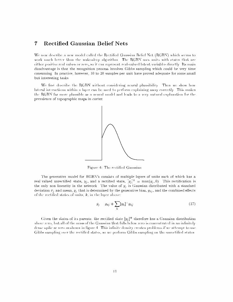
Figure 4: The recti�ed Gaussian.

The generative model for RGBN's consists of multiple layers of units each of which has areal-valued unrecti�ed state, yj , and a recti�ed state, [yj]

+ = max(yj; 0). This recti�cation isthe only non-linearity in the network. The value of yj is Gaussian distributed with a standarddeviation �j and mean, yj that is determined by the generative bias, g0j, and the combined e�ectsof the recti�ed states of units, k, in the layer above:

yj = g0j +Xk

[yk]+gkj (17)

Given the states of its parents, the recti�ed state [yj ]+ therefore has a Gaussian distribution

above zero, but all of the mass of the Gaussian that falls below zero is concentrated in an in�nitelydense spike at zero as shown in �gure 4. This in�nite density creates problems if we attempt to useGibbs sampling over the recti�ed states, so we perform Gibbs sampling on the unrecti�ed states.

11

7.1 Sampling from the posterior distribution in an RGBN

Consider a unit, j, in some intermediate layer of a multi-layer RGBN (see �gure 3). Suppose thatwe �x the unrecti�ed states of all the other units in the net.4 To perform Gibbs sampling, we needto stochastically select a value for yj according to its posterior distribution given the unrecti�edstates of all the other units.

If we think in terms of energies that correspond to negative log probabilities, the recti�edstates of the units in the layer above contribute a quadratic energy term by determining yj. Theunrecti�ed states of units, i, in the layer below contribute nothing if [yj ]+ is 0, and if [yj]+ ispositive they each contribute a quadratic term because of the e�ect of [yj]+ on yi.

E(yj) =(yj � yj)

2

2�2j+Xi

(yi �P

h[yh]+ghi)

2

2�2i(18)

where h is an index over all the units in the same layer as j including j itself, so yj in uencesthe right hand side of the Eq. 18 via [yj ]

+ = max(yj ; 0). Terms that do not depend on yj havebeen omitted from Eq. 18. For values of yj below zero there is a quadratic energy function whichleads to a Gaussian posterior distribution. The same is true for values of yj above zero, but it isa di�erent quadratic (see �gure 5b). The Gaussian posterior distributions corresponding to thetwo quadratics must agree at yj = 0 (�gure 5a). Because the posterior distribution is piecewiseGaussian it is possible to perform Gibbs sampling exactly and fairly e�ciently (see appendix).

−3 −2 −1 0 1 2 3

a

p(y)

−3 −2 −1 0 1 2 3y

E(y

)

b

Top−down contribution

Bottom−up contribution

Figure 5: a) Schematic of the posterior density of an unrecti�ed state of a unit. b) Bottom-upand top-down energy functions corresponding to a.

4Actually it is only necessary to �x the unrecti�ed states of units in the layer above that send a generativeconnection to j, units in the layer below to which j sends a generative connection, and units in the same layer thatsend generative connections to units directly a�ected by j.

12

7.2 Learning the parameters of a RGBN

Given samples from the posterior distribution, the generative weights of a RGBN can be learnedby using the online delta rule to perform gradient ascent in the log likelihood of the data:

�gji = �[yj ]+(yi � yi) (19)

The variance of the local Gaussian noise of each unit, �2j , can be learned by an online rule:

��2j = �[(yj � yj)2 � �2j ] (20)

Alternatively, �2j can be �xed at 1 for all hidden units and the e�ective local noise level can becontrolled by scaling the generative weights.

7.3 The Role of Lateral Connections

Lee and Seung (1997) introduced a clever trick in which lateral connections are used to handleexplaining away e�ects. The trick is most easily understood for a linear generative model of thetype used in factor analysis. One contribution, Ebelow, to the energy of the state of the network isthe squared di�erences between the states of the units in the bottom layer, yj , and the top-downexpectations, yj generated by the states of units in the layer above. Another contribution, Eabove,is the squared di�erence between the states in the top layer, yk, and their top-down expectations,yk. Assuming the local noise models for the lower layer units all have unit variance, and ignoringbiases and constant terms that are una�ected by the states of the units

Ebelow =Xj

(yj � yj)2 =

Xj

(yj �P

kykgkj)2 (21)

This expression can be rearranged to give

Ebelow =Xj

y2j � 2Xk

ykXj

yjgkj �Xk

Xl

ykyl(�P

jgkjglj) (22)

Setting rjk = gkj and mkl = �Pj gkjglj we get

Ebelow =Xj

y2j � 2Xk

ykXj

yjrjk �Xk

ykXl

ylmkl (23)

The way in which Ebelow depends on each activity in the layer above, yk, is determined by thesecond and third terms in Eq. 23. So if unit k computes

Pj yjrjk using the bottom-up recognition

connections, andP

l ylmkl using the lateral connections it has all of the information it requiresabout Ebelow to perform Gibbs sampling in the potential function Ebelow + Eabove (see �gure 6).

If we are willing to use Gibbs sampling, Seung's trick allows a proper implementation offactor analysis in a neural network because it makes it possible to sample from the full covarianceposterior distribution in the hidden state space. Seung's trick can also be used in a RGBN andit eliminates the most neurally implausible aspect of this model which is that a unit in one layerappears to need to send both its state y and the top-down prediction of its state y to units in the

13

k

glj

rjkrjl

gkj

j

lmkl

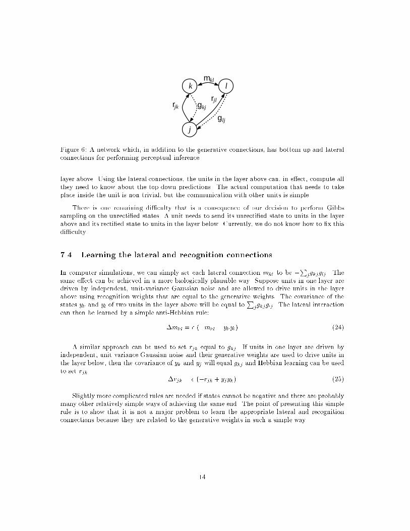
Figure 6: A network which, in addition to the generative connections, has bottom-up and lateralconnections for performing perceptual inference.

layer above. Using the lateral connections, the units in the layer above can, in e�ect, compute allthey need to know about the top-down predictions. The actual computation that needs to takeplace inside the unit is non-trivial, but the communication with other units is simple.

There is one remaining di�culty that is a consequence of our decision to perform Gibbssampling on the unrecti�ed states. A unit needs to send its unrecti�ed state to units in the layerabove and its recti�ed state to units in the layer below. Currently, we do not know how to �x thisdi�culty.

7.4 Learning the lateral and recognition connections

In computer simulations, we can simply set each lateral connection mkl to be �Pjgkjglj . Thesame e�ect can be achieved in a more biologically plausible way. Suppose units in one layer aredriven by independent, unit-variance Gaussian noise and are allowed to drive units in the layerabove using recognition weights that are equal to the generative weights. The covariance of thestates yk and yl of two units in the layer above will be equal to

Pjgkjglj . The lateral interaction

can then be learned by a simple anti-Hebbian rule:

�mkl = � (�mkl � ykyl) (24)

A similar approach can be used to set rjk equal to gkj. If units in one layer are driven byindependent, unit-variance Gaussian noise and their generative weights are used to drive units inthe layer below, then the covariance of yk and yj will equal gkj and Hebbian learning can be usedto set rjk

�rjk = � (�rjk + yjyk) (25)

Slightly more complicated rules are needed if states cannot be negative and there are probablymany other relatively simple ways of achieving the same end. The point of presenting this simplerule is to show that it is not a major problem to learn the appropriate lateral and recognitionconnections because they are related to the generative weights in such a simple way.

14

7.5 A reason for topographic maps

It is infeasible to interconnect all pairs of units in a cortical area. If we assume that direct lateralinteractions (or interactions mediated by interneurons) are primarily local, then widely separatedunits will not have the connections required for explaining away. Consequently the computation ofthe posterior distribution will be incorrect unless the generative weight vectors of widely separatedunits are orthogonal. If the generative weights are constrained to be positive, the only way twovectors can be orthogonal is for one to have zeros where the other has non-zeros. It follows thatwidely separated units must attend to di�erent parts of the image and units can only attendto overlapping patches if they are laterally interconnected. We have not described a mechanismfor the formation of topographic maps, but we have given a good computational reason for theirexistence.

8 Results on a toy task

A simple problem that illustrates the need for sparse distributed representations is the noisy barsproblem (Hinton et al., 1995). Consider the following multi-stage generative model for K � Kimages. The top level decides with equal probabilities whether the image will consist solely ofvertical or horizontal bars. Given this choice, the second level decides independently for each ofthe K bars of the appropriate orientation whether it is present or not, with a probability of 0.3 ofbeing present. If a bar is present, it's intensity is determined by a uniformly distributed randomvariable. Finally, independent Gaussian noise is added to each pixel in the image. Sample imagesgenerated from this process are shown in �gure 7a.

We trained a three-layer RGBN consisting of 36 visible units, 24 units in the �rst hidden layerand 1 unit in the second hidden layer on the 6�6 bars problem. While there are 126 combinationsof possible bars (not accounting for the real-valued intensities and Gaussian noise), a distributedrepresentation with only 12 hidden units in the �rst layer can capture the presence or absenceof each bar. With this representation in the �rst hidden layer, the second hidden layer can thencapture higher-order structure by detecting that vertical bars are correlated with other verticalbars and not with horizontal bars.

The network was trained for 10 passes through a data set of 1000 images using a di�erent,random order for each pass. For each image we used 16 iterations of Gibbs sampling to approximatethe posterior distribution over hidden states. Each iteration consisted of sampling every hiddenunit once in a �xed order. The states on every other iteration were used for learning, with alearning rate of 0.1 and a weight decay parameter of 0.01. Since the top level of the generativeprocess makes a discrete decision between vertical and horizontal bars, we tried both the RGBNand a trivial extension of the RGBN in which the top level unit saturates both at 0 and 1. Thisresulted in slightly cleaner representations at the top level. Results were relatively insensitive toother parametric changes.

After learning, each of the 12 possible bars is represented by a separate unit in the �rsthidden layer (�gure 8c). The remaining hidden units in that layer are kept inactive throughstrong inhibitory biases (�gure 8b). The unit in the top hidden layer strongly excites the verticalbar units in the �rst hidden layer, and inhibits the horizontal bar units. Indeed, when presentedwith images and allowed to randomly sample its states for 10 Gibbs samples, the top unit is

15

a b

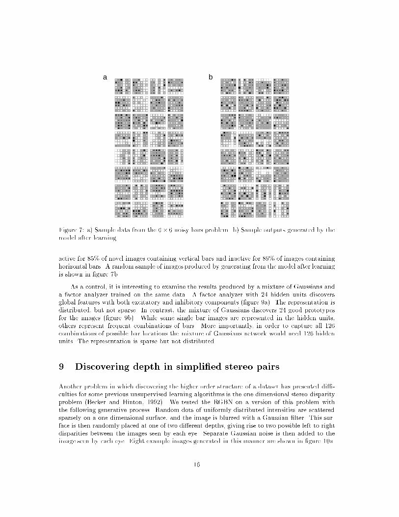
Figure 7: a) Sample data from the 6� 6 noisy bars problem. b) Sample outputs generated by themodel after learning.

active for 85% of novel images containing vertical bars and inactive for 89% of images containinghorizontal bars. A random sample of images produced by generating from the model after learningis shown in �gure 7b.

As a control, it is interesting to examine the results produced by a mixture of Gaussians anda factor analyzer trained on the same data. A factor analyzer with 24 hidden units discoversglobal features with both excitatory and inhibitory components (�gure 9a). The representation isdistributed, but not sparse. In contrast, the mixture of Gaussians discovers 24 good prototypesfor the images (�gure 9b). While some single bar images are represented in the hidden units,others represent frequent combinations of bars. More importantly, in order to capture all 126combinations of possible bar locations the mixture of Gaussians network would need 126 hiddenunits. The representation is sparse but not distributed.

9 Discovering depth in simpli�ed stereo pairs

Another problem in which discovering the higher order structure of a dataset has presented di�-culties for some previous unsupervised learning algorithms is the one-dimensional stereo disparityproblem (Becker and Hinton, 1992). We tested the RGBN on a version of this problem withthe following generative process. Random dots of uniformly distributed intensities are scatteredsparsely on a one-dimensional surface, and the image is blurred with a Gaussian �lter. This sur-face is then randomly placed at one of two di�erent depths, giving rise to two possible left-to-rightdisparities between the images seen by each eye. Separate Gaussian noise is then added to theimage seen by each eye. Eight example images generated in this manner are shown in �gure 10a.

16

a

b

c

Figure 8: Generative weights of a three-layered RGBN after being trained on the noisy barsproblem. a) Weights from the top layer hidden unit to the 24 middle-layer hidden units. b) Biasesof the middle layer hidden units, and c) weights from the hidden units to the 6� 6 visible array,arranged in the same manner as in a).

Using the very same architecture and training parameters as in the previous example, wetrained an RGBN on images from this stereo disparity problem. As in the previous example, eachof the 24 hidden units in the �rst hidden layer was connected to the entire array of 36 visibleunits, i.e. it had inputs from both eyes. Twelve of these hidden units learned to become localleft-disparity detectors, while the other twelve became local right-disparity detectors (�gure 11c).Unlike the previous problem, in which there were too many hidden units for the problem, herethere were too few for the 18 pixel locations. The unit in the second hidden layer has positiveweights connecting it to leftward disparity detecting hidden units in the layer below, and negativeweights for the rightward units (�gure 11a). When presented with novel input images the top unitis active for 87% of images with leftward disparity and inactive for 91% of images with rightwarddisparity. A random sample of images generated by the model after learning is shown in �gure 10b.

10 Discussion

The units used in an RGBN have a number of di�erent properties and it is interesting to ask whichof these properties are essential and which are arbitrary. If we want to achieve neural plausibilityby using lateral interactions to handle explaining away, it is essential that Gaussian noise is usedto convert yj into yj in the generative model. Without this, the expression for Ebelow in Eq. 21would not be quadratic and it would not be possible to take the summation over j inside thesummation over k in Eq. 23.

In the RGBN, there are two linear regimes. Either [y]+ = y or [y]+ = 0 depending on the

17

a b

Figure 9: a) Generative weights of a factor analyzer with 24 hidden units trained on the samedata as the RGBN. b) Generative weights of a mixture of 24 Gaussians trained on the same data.

value of y. Clearly, the idea can be generalized to any number of regimes and the only constrainton each regime is that it should be linear so that exact Gibbs sampling is possible5. If we usetwo constant regimes and replace [y]+ by a binary output s which is 1 when y is positive and0 otherwise we get a \probit" belief net that is very similar to the logistic belief net describedin section 5 but has the advantage that the lateral connection trick can be used for perceptualinference.

Probit units and linear or recti�ed linear units can easily be combined in the same networkby making the output of a unit of one type contribute to the top-down expectation, y of a unit ofthe other type. They can also be combined in a more interesting way. The discrete output of aprobit unit si can multipy the output of a linear unit yj and exact Gibbs sampling is still feasible.This allows the probit unit to decide whether yj should be used without in uencing the value ofyj if it is used. This is useful if, for example, yj represents the size of an object and si representswhether it exists.

If a probit unit and a linear unit share the same y value their combination is exactly a recti�edlinear unit. If they merely share the same y value but use independent local noise to get di�erenty values, we get a softer blending of the linear and the constant regime. It is also feasible tocombine a generalization of the probit unit that uses its y value to deterministically pick one ofm possibilities with a generalization of the linear unit that has m di�erent linear regimes. This isa generative version of the mixture of experts model (Jacobs et al., 1991).

The RGBN is a particularly interesting case because the in�nite density of [y]+ at 0 meansthat it is very cheap, in coding terms, for units to have outputs of 0, so the network developssparse representations. Each hidden unit can be viewed as a linear basis function for representingthe states in the layer below, but only a subset of these basis functions are used for a given datapoint. Because the network can select which basis functions are appropriate for the data, it can

5By using a few linear regimes we can crudely approximate units whose output is a smooth non-linear functionof y (Frey, 1997) and still perform exact Gibbs sampling.

18

a b

Figure 10: a) Sample data from the simpli�ed stereo disparity problem. The top and bottom rowof each 2 � 18 image are the inputs to the left and right eye, respectively. Notice that the highpixel noise makes it di�cult to infer the disparity in some images. b) Sample outputs generatedby the model after learning.

tailor a basis function to a rare, complex feature without incurring the cost of representing theprojection onto this basis function for every single data point. Other methods for developing sparserepresentations (Olshausen and Field, 1996; Lee and Seung, 1997) rely on generative models thathave a non-Gaussian local noise model for the hidden units, so the lateral connection trick doesnot work when they are generalized to multiple hidden layers.

It remains to be seen how RGBN's fare on larger, more realistic datasets. We hope thatthey will be able to discover many di�erent sources of information about properties like surfacedepth and surface orientation in natural images and that their method of performing perceptualinference will combine these di�erent sources correctly when interpreting a single image.

It is possible that the number of iterations of Gibbs sampling required will increase signi�cantlywith the size of the input and the number of layers. This would certainly happen if interpretingan image was a typical combinatorial optimization problem in which the best solution to one partof the problem considered in isolation is usually incompatible with the best solution to anotherpart of the problem. This is called a \frustrated" system and is just what vision is not like. It isgenerally easier to interpret two neighboring patches of an image than to interpret one patch inisolation because context almost always facilitates interpretation. Imagine two separate networks,one for each image patch. When we interconnect the networks, they should settle faster, notslower. Simulations will demonstrate whether this conjecture is correct.

An interesting way to reduce the time required for Gibbs sampling is to initialize the stateof the network to an interpretation of the data that is approximately correct. For data thathas temporal coherence this could be done by using a predictive causal model for initialization.For data that lacks temporal coherence it is still possible to initialize the network sensibly bylearning a separate set of bottom-up connection strengths which are used in a single pass forinitialization. These connection strengths can be learned using the delta rule, where the resultsof Gibbs sampling de�ne the desired initial states. The initialization connections save time bycaching an approximation to the results of Gibbs sampling on previous, similar data.

19

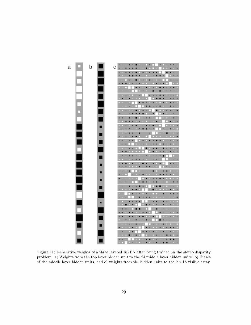
a b c

Figure 11: Generative weights of a three-layered RGBN after being trained on the stereo disparityproblem. a) Weights from the top layer hidden unit to the 24 middle-layer hidden units. b) Biasesof the middle layer hidden units, and c) weights from the hidden units to the 2� 18 visible array.

20

Acknowledgments

We thank Peter Dayan, Brendan Frey, Geo�rey Goodhill, Michael Jordan, David MacKay,Radford Neal and Mike Revow for numerous insights and David Mackay for greatly improvingthe manuscript. The research was funded by grants from the Canadian Natural Science andEngineering Research Council and the Ontario Information Technology Research Center. GEH isthe Nesbitt-Burns fellow of the Canadian Institute for Advanced Research.

21

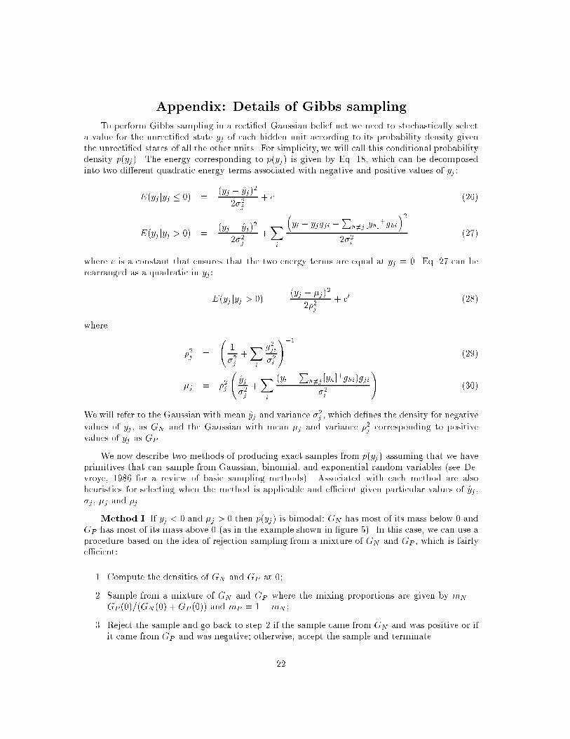
Appendix: Details of Gibbs sampling

To perform Gibbs sampling in a recti�ed Gaussian belief net we need to stochastically selecta value for the unrecti�ed state yj of each hidden unit according to its probability density giventhe unrecti�ed states of all the other units. For simplicity, we will call this conditional probabilitydensity p(yj). The energy corresponding to p(yj) is given by Eq. 18, which can be decomposedinto two di�erent quadratic energy terms associated with negative and positive values of yj :

E(yj jyj � 0) =(yj � yj)2

2�2j+ c (26)

E(yj jyj > 0) =(yj � yj)2

2�2j+Xi

�yi � yjgji �

Ph6=j [yh]

+ghi

�22�2i

(27)

where c is a constant that ensures that the two energy terms are equal at yj = 0. Eq. 27 can berearranged as a quadratic in yj:

E(yj jyj > 0) =(yj � �j)2

2�2j+ c0 (28)

where

�2j =

1

�2j+Xi

g2ji�2i

!�1

(29)

�j = �2j

yj�2j

+Xi

(yi �P

h6=j [yh]+ghi)gji

�2i

!(30)

We will refer to the Gaussian with mean yj and variance �2j , which de�nes the density for negative

values of yj , as GN and the Gaussian with mean �j and variance �2j corresponding to positivevalues of yj as GP .

We now describe two methods of producing exact samples from p(yj) assuming that we haveprimitives that can sample from Gaussian, binomial, and exponential random variables (see De-vroye, 1986 for a review of basic sampling methods). Associated with each method are alsoheuristics for selecting when the method is applicable and e�cient given particular values of yj ,�j, �j and �j .

Method I. If yj < 0 and �j > 0 then p(yj) is bimodal: GN has most of its mass below 0 andGP has most of its mass above 0 (as in the example shown in �gure 5). In this case, we can use aprocedure based on the idea of rejection sampling from a mixture of GN and GP , which is fairlye�cient:

1. Compute the densities of GN and GP at 0;

2. Sample from a mixture of GN and GP where the mixing proportions are given by mN =GP (0)=(GN (0) + GP (0)) and mP = 1�mN ;

3. Reject the sample and go back to step 2 if the sample came from GN and was positive or ifit came from GP and was negative; otherwise, accept the sample and terminate.

22

Since the probability of rejecting a sample is less than 0.5, the mean time for this procedure toproduce an accepted sample from p(yj) is at most two steps.

Method II. If yj > 0 or �j < 0 then it becomes necessary to sample from the tail of GN ,GP or both, and the above procedure may be very ine�cient. The following is a more e�cientprocedure which can be used in this case:

1. Compute the mass of GN below 0, weighted by the mixing proportion as previously de�ned

MN = mN

Z 0

�1

GN (y) dy (31)

and similarly for the mass of GP above 0. (Of course, this integral cannot be solved analyt-ically and will require a call to the erf function);

2. With probabilityMN=(MN +MP ) stochastically decide to sample from the negative side ofGN , otherwise select the positive side of GP . Call this selection G and the side we want tosample from the \correct side" of G.

3. If the correct side of G has a substantial probability mass, for example, if G = GN andyj=�j < 1=2, then sample from G repeatedly, accepting the �rst sample that comes from thecorrect side of G.

4. If the correct side of G does not have a substantial probability mass, that is, if it is the\tail" of a Gaussian, then we upper bound it by an exponential distribution and again userejection sampling. Assuming GP was selected in step 2, let F (y) be an exponential densityin y: F (y) = 1

�e�y=�, with decay constant � = ��2j=�j, chosen to match the decay of the

Gaussian tail at 0. (To sample from GN we simply reverse the sign of y and de�ne � in termsof �j and yj .) Sample y from F (y) until y is accepted, where the acceptance probability isG(y)F (0)=F (y)G(0). This acceptance probability is obtained by scaling the Gaussian tailto match the exponential at y = 0, and then computing the ratio of the scaled Gaussian tailat y to the exponential at y.

The condition in step 3 of this method ensures that the mean time to produce an accepted samplefrom p(yj) will be at most about 3 steps. For step 4 the quality of the exponential bound (andtherefore the mean number of samples until acceptance) depends on how far in the tail of theGaussian we are sampling. For a tail starting from 1/2 standard deviations from the mean of theGaussian, the acceptance probability for the exponential approximation is on average about 0.4,and this probability increases for Gaussian tails further from the mean.

Finally, we should point out that these are just some of the methods that can be used tosample from p(yj). Implementations using other sampling methods, such as adaptive rejectionsampling (Gilks and Wild, 1992), are also possible.

23

References

Barlow, H. (1989). Unsupervised learning. Neural Computation, 1:295{311.

Becker, S. and Hinton, G. (1992). A self-organizing neural network that discovers surfaces inrandom-dot stereograms. Nature, 355:161{163.

Bishop, C. M., Svensen, M., and Williams, C. K. I. (In Press). GTM: A principled alternative tothe self-organizing map. Neural Computation.

Dempster, A., Laird, N., and Rubin, D. (1977). Maximum likelihood from incomplete data viathe EM algorithm. J. Royal Statistical Society Series B, 39:1{38.

Devroye, L. (1986). Non-uniform Random Variate Generation. Springer-Verlag, New York.

Durbin, R. and Willshaw, D. (1987). An analogue approach to the travelling salesman problemusing an elastic net method. Nature, 326(16):689{691.

Everitt, B. S. (1984). An Introduction to Latent Variable Models. Chapman and Hall, London.

Frey, B. J. (1997). Continuous sigmoidal belief networks trained using slice sampling. In Mozer,M., Jordan, M., and Petsche, T., editors, Advances in Neural Information Processing Systems

9. MIT Press, Cambridge, MA.

Geman, S. and Geman, D. (1984). Stochastic relaxation, Gibbs distributions, and the Bayesianrestoration of images. IEEE Transactions on Pattern Analysis and Machine Intelligence,6:721{741.

Gilks, W. R. and Wild, P. (1992). Adaptive rejection sampling for gibbs sampling. Applied

Statistics, 41:337{348.

Gregory, R. L. (1970). The Intelligent Eye. Wiedenfeld and Nicolson, London.

Hinton, G. E., Dayan, P., Frey, B. J., and Neal, R. M. (1995). The wake-sleep algorithm forunsupervised neural networks. Science, 268:1158{1161.

Hinton, G. E. and Sejnowski, T. J. (1983). Optimal perceptual Inference. In Proc. of the IEEE

Computer Society Conf. on Computer Vision and Pattern Recognition, pages 448{453. Wash-ington, DC.

Hinton, G. E. and Sejnowski, T. J. (1986). Learning and relearning in Boltzmann machines. InRumelhart, D. E. and McClelland, J. L., editors, Parallel Distributed Processing: Explorationsin the Microstructure of Cognition. Volume 1: Foundations. MIT Press, Cambridge, MA.

Horn, B. K. P. (1977). Understanding image intensities. Arti�cial Intelligence, 8:201{231.

Jacobs, R. A., Jordan, M. I., Nowlan, S. J., and Hinton, G. E. (1991). Adaptive mixture of localexperts. Neural Computation, 3:79{87.

Kohonen, T. (1982). Self-organized formation of topologically correct feature maps. Biological

Cybernetics, 43:59{69.

Lee, D. D. and Seung, H. S. (1997). Unsupervised learning by convex and conic coding. In Mozer,M., Jordan, M., and Petsche, T., editors, Advances in Neural Information Processing Systems

9. MIT Press, Cambridge, MA.

24

Lewicki, M. S. and Sejnowski, T. J. (1997). Bayesian unsupervised learning of higher orderstructure. In Mozer, M., Jordan, M., and Petsche, T., editors, Advances in Neural Information

Processing Systems 9. MIT Press, Cambridge, MA.

Mumford, D. (1994). Neuronal architectures for pattern-theretic problems. In Koch, C. andDavis, J. L., editors, Large-Scale Neuronal Theories of the Brain, pages 125{152. MIT Press,Cambridge, MA.

Neal, R. M. (1992). Connectionist learning of belief networks. Arti�cial Intelligence, 56:71{113.

Neal, R. M. and Dayan, P. (1996). Factor analysis using delta-rule wake-sleep learning. TechnicalReport No. 9607 Dept. of Statistics, University of Toronto.

Olshausen, B. A. and Field, D. J. (1996). Emergence of simple-cell receptive �eld properties bylearning a sparse code for natural images. Nature, 381:607{609.

Pearl, J. (1988). Probabilistic Reasoning in Intelligent Systems: Networks of Plausible Inference.Morgan Kaufmann, San Mateo, CA.

Rumelhart, D. and Zipser, D. (1985). Feature discovery by competitive learning. Cognitive Science,9:75{112.

Rumelhart, D. E., Hinton, G. E., and Williams, R. J. (1986). Learning internal representationsby back-propagating errors. Nature, 323:533{536.

25