University of Groningen

A survey on the analysis and control of evolutionary matrix gamesRiehl, James Robert; Ramazi, Pouria; Cao, Ming

Published in:Annual Reviews in Control

DOI:10.1016/j.arcontrol.2018.04.010

IMPORTANT NOTE: You are advised to consult the publisher's version (publisher's PDF) if you wish to cite fromit. Please check the document version below.

Document VersionFinal author's version (accepted by publisher, after peer review)

Publication date:2018

Link to publication in University of Groningen/UMCG research database

Citation for published version (APA):Riehl, J. R., Ramazi, P., & Cao, M. (2018). A survey on the analysis and control of evolutionary matrixgames. Annual Reviews in Control, 45, 87-106. https://doi.org/10.1016/j.arcontrol.2018.04.010

CopyrightOther than for strictly personal use, it is not permitted to download or to forward/distribute the text or part of it without the consent of theauthor(s) and/or copyright holder(s), unless the work is under an open content license (like Creative Commons).

The publication may also be distributed here under the terms of Article 25fa of the Dutch Copyright Act, indicated by the “Taverne” license.More information can be found on the University of Groningen website: https://www.rug.nl/library/open-access/self-archiving-pure/taverne-amendment.

Take-down policyIf you believe that this document breaches copyright please contact us providing details, and we will remove access to the work immediatelyand investigate your claim.

Downloaded from the University of Groningen/UMCG research database (Pure): http://www.rug.nl/research/portal. For technical reasons thenumber of authors shown on this cover page is limited to 10 maximum.

Download date: 28-11-2021

A Survey on the Analysis and Control of Evolutionary Matrix Games

James Riehla,∗, Pouria Ramazib, Ming Caoc,∗

aDepartment of Electrical and Systems Engineering, Washington University in St. Louis, USAbDepartment of Mathematical and Statistical Sciences, University of Alberta, Canada

cFaculty of Science and Engineering, University of Groningen, Netherlands

Abstract

In support of the growing interest in how to efficiently influence complex systems of interacting self-interestedagents, we present this review of fundamental concepts, emerging research, and open problems related to theanalysis and control of evolutionary matrix games, with particular emphasis on applications in social, economic,and biological networks.

Keywords: evolutionary games, population dynamics, equilibrium convergence, control strategies

Contents

1 Introduction 2

2 Evolutionary matrix games on networks 32.1 Networks, games, and payoffs . . . . . . . . . . . . . . . . . . . . . . . . . . . . . . . . . . . . 42.2 Discrete-time evolutionary dynamics . . . . . . . . . . . . . . . . . . . . . . . . . . . . . . . . . 4

2.2.1 Best-response update rule . . . . . . . . . . . . . . . . . . . . . . . . . . . . . . . . . . 42.2.2 Imitation update rule . . . . . . . . . . . . . . . . . . . . . . . . . . . . . . . . . . . . . 62.2.3 Proportional imitation update rule . . . . . . . . . . . . . . . . . . . . . . . . . . . . . . 6

2.3 Continuous time evolutionary dynamics . . . . . . . . . . . . . . . . . . . . . . . . . . . . . . . 62.3.1 Derivation of the replicator dynamics . . . . . . . . . . . . . . . . . . . . . . . . . . . . 72.3.2 Best-response dynamics . . . . . . . . . . . . . . . . . . . . . . . . . . . . . . . . . . . 9

3 Equilibrium convergence and stability 103.1 Infinite well-mixed populations (continuous-time continuous-state dynamics) . . . . . . . . . . . 10

3.1.1 Equilibrium states . . . . . . . . . . . . . . . . . . . . . . . . . . . . . . . . . . . . . . 103.1.2 Lyapunov stable states . . . . . . . . . . . . . . . . . . . . . . . . . . . . . . . . . . . . 113.1.3 Asymptotically stable states . . . . . . . . . . . . . . . . . . . . . . . . . . . . . . . . . 113.1.4 Globally asymptotically stable states . . . . . . . . . . . . . . . . . . . . . . . . . . . . . 123.1.5 Convergence results . . . . . . . . . . . . . . . . . . . . . . . . . . . . . . . . . . . . . 133.1.6 Folk Theorem . . . . . . . . . . . . . . . . . . . . . . . . . . . . . . . . . . . . . . . . . 13

3.2 Infinite structured populations (continuous-time continuous-state dynamics) . . . . . . . . . . . . 143.3 Finite structured populations (discrete-time discrete-state dynamics) . . . . . . . . . . . . . . . . 14

3.3.1 Imitation . . . . . . . . . . . . . . . . . . . . . . . . . . . . . . . . . . . . . . . . . . . 143.3.2 Best-response . . . . . . . . . . . . . . . . . . . . . . . . . . . . . . . . . . . . . . . . . 15

4 Control strategies 164.1 Infinite well-mixed populations . . . . . . . . . . . . . . . . . . . . . . . . . . . . . . . . . . . . 164.2 Finite structured populations . . . . . . . . . . . . . . . . . . . . . . . . . . . . . . . . . . . . . 17

4.2.1 Unique convergence for a class of coordinating agents . . . . . . . . . . . . . . . . . . . 174.2.2 Direct strategy control . . . . . . . . . . . . . . . . . . . . . . . . . . . . . . . . . . . . 184.2.3 Incentive-based control . . . . . . . . . . . . . . . . . . . . . . . . . . . . . . . . . . . . 19

∗Corresponding author

Preprint submitted to Annual Reviews in Control Wednesday 13th June, 2018

5 Open Problems 215.1 Infinite well-mixed populations . . . . . . . . . . . . . . . . . . . . . . . . . . . . . . . . . . . . 215.2 Finite structured populations . . . . . . . . . . . . . . . . . . . . . . . . . . . . . . . . . . . . . 22

6 Concluding Remarks 22

Appendix A 2-player matrix games 24

Appendix B Nash equilibrium 25

Appendix C Categorization of 2 by 2 matrix games 25

Appendix D Analyses of the replicator dynamics for 2x2 games 26

Appendix E Evolutionary stability and neutral stability 26

Appendix F Lotka-Volterra equation 28

Appendix G Convergence proofs for asynchronous best-response dynamics 29

1. Introduction

Whether humans in a community, ants in a colony, or neurons in a brain, simple decisions or actions byinteracting individuals can lead to complex and unpredictable outcomes in a population. The study of such systemstypically presents a choice between micro- and macro-scale analysis. While there exist intricate micro-models ofhuman decision processes, ant behaviors, and single neurons, assembling these high-dimensional components on alarge scale most often results in models that are impenetrable to analysis, and therefore unlikely to reveal any usefulproperties of the collective dynamics. On the other hand, research on these systems at a broader scale, perhapssubject to substantial simplification of the agent-level dynamics, can help to characterize critical properties suchas convergence, stability, controllability, robustness, and performance [1]. This helps to explain the recent andremarkable trend towards network-based analysis across various disciplines in engineering and the biological andsocial sciences, which has led to several important discoveries related to system dynamics on complex networks[2, 3, 4, 5]. For control scientists and engineers, these results facilitate the study of timely and challenging issuesrelated to social, economic, and biological sciences from a control-theoretic perspective.

Evolutionary game theory has emerged as a vital toolset in the investigation of these topics. Originally pro-posed as a framework to study behaviors such as ritualized fighting in animals [6], it has since been widelyadopted in various disciplines outside of biology. The primary innovation of evolutionary game theory is thatrather than assuming high levels of rationality in individual choices, perhaps a questionable assumption even forhumans, strategies and behaviors propagate through populations via dynamic processes. In the biological world,this propagation is manifested through survival of the fittest and reproductive processes, which are widely mod-eled using population dynamics [1, 7, 8]. Systems of first-order differential equations such as replicator dynamics(RD) provide an elegant and powerful means to investigate collective behaviors, assuming infinite and well-mixedpopulations. While these assumptions can lead to reasonable approximations for large, dense populations of or-ganisms, in many other real-world networks, the structure and range of individual interactions plays a major rolein the dynamics [9]. Fortunately, it is still possible to study replicator-like dynamics in populations connected bynetworks [10], and it turns out that certain models of imitation reduce exactly to RD in the limit of large networks[11]. Other seemingly more rational decision models such as best-response dynamics [12, 13, 14, 15, 16] also fitnaturally into a network setting, as we will discuss in Section 2.

An extensive literature has emerged in the field of evolutionary games on networks, particularly regarding thequestion of how cooperation can evolve and persist under various conditions and in various population structures[17, 18, 19]. In this article, rather than survey these works, we will present only some fundamental results inclassical evolutionary game dynamics, before discussing some recent developments in the areas of equilibriumconvergence and control. Specifically, we set out to achieve three primary goals. First, we aim to introduce thepowerful analytical tools of evolutionary game theory to control scientists and engineers not already familiar withthe topic. Second, we provide a brief survey of some recent results in the analysis and control of evolutionarymatrix games. Third, we discuss some current challenges and open problems in the field for the consideration ofinterested researchers.

2

We emphasize that, although game theory and evolutionary game theory are receiving increasing attentionas design tools for implementing distributed optimization in industrial and technological systems [20, 21, 22],including water distribution [23, 24], wireless communication [25], optical networks [26], and transportation [27],we focus this survey specifically on the analysis and control of self-organized systems whose constituents arenot necessarily subject to design. This stands apart from some ongoing research which aims at engineering thedynamics governing a population of programmable individuals, e.g., robots, in order to drive the state of thesystem to a desired state. We refer the reader to surveys such as [21, 28] for detailed discussions on this separatebut complementary topic. In contrast, typical individuals we model in this paper such as humans, firms, animals,and neurons are clearly not programmable in the same sense, and even if they were, attempting to do so wouldlikely raise ethical concerns. Rather, for the dynamics of these individuals, we take existing models proposedby biologists, sociologists, and economists, and perform convergence and stability analysis, which deepens ourunderstanding of their collective behaviors. As the next step, by exploiting the limited freedom in modifying thedynamics of the individuals, such as providing incentives, we investigate attempts to guide such populations todesired states, beneficial to the overall group of individuals. The results, however, are not necessarily limited tosocial or biological populations, and could potentially be applied to the design of multi-agent systems to performa group task in an uncertain, noisy situation that requires decision-making by the agents [29, 30].

2. Evolutionary matrix games on networks

In the context of game theory, a game is a simple model of an interaction between two or more players inwhich individuals’ payoffs depend on the actions or strategies of each player. A matrix game is a 2-player game inwhich each player selects from a finite set of strategies and the payoff depends only on the strategies selected bythe agents, such that all possible payoff outcomes of the game can be written in matrix form. See Appendix B forthe formal definition of a Nash equilibrium and some of its refinements and Appendix A for a brief introductionto 2-player matrix games.

As an illustrative example, we consider one of the most famous games in all of game theory, the prisoner’sdilemma (PD). In the original formulation, two suspects are arrested for a crime, and the police do not have enoughevidence to convict either suspect, so they question them separately [31]. Each suspect can either cooperate (C)with the other by not answering any questions or defect (D) by testifying against the other suspect. The sentencesfor the two suspects depend on both of their actions, as shown in the following payoff matrix, in which one suspectchooses a row and their opponent chooses a column:

πPD =

( C DC −2 −5D 0 −4

).

Since this is a symmetric game, the payoff matrix is identical from the perspective of both players. If both suspectscooperate, the judge is lenient due to a lack of evidence that either suspect committed the crime and gives bothsuspects a 2-year sentence. However, if suspect 1 cooperates and suspect 2 defects, then the evidence points tosuspect 1 who must serve the full sentence of 5 years while suspect 2 serves no prison time, and vice versa. Finally,if both suspects defect, the judge assumes one of them is guilty but without knowing which one, sentences themboth to 4 years in prison.

The dilemma arises from the fact that although mutual cooperation would result in the best combined outcome,there is always a temptation for each suspect to defect to get a shorter sentence, resulting in a state of mutualdefection. In other words, defection is the best response to both cooperation and defection by the other suspect. Astate in which both players are playing best responses to each other is called a Nash equilibrium. See AppendixC for a complete categorization of 2 × 2 symmetric matrix games, which are the primary focus in this article.However, matrix games in general may have an arbitrary number of strategies, and we will also include someresults about this more general case.

Evolutionary game theory extends classical game theory, which deals mostly with static concepts, by relaxingthe assumption of perfect rationality and instead assuming that strategies propagate through a population throughsome dynamic process. Of the many different dynamics proposed for evolutionary games, we focus this articleon two of the most widely studied models: imitation and best-response. In imitation dynamics, players adoptthe strategy of their most successful neighbors, whereas in best-response dynamics, players choose strategiesthat will maximize their own respective payoffs. In summary, an evolutionary matrix game models the dynamicinteractions of a population of agents, each of which chooses from a finite set of actions, receiving payoffs thatdepend on these actions. Based on the application and research goals, these dynamics are commonly expressed

3

either as systems of first-order ordinary differential equations (ODEs), as in RD, described in Section 2.3, or asdiscrete-time agent-based update rules on networks, defined in Section 2.1.

Analysis of evolutionary matrix games can help to understand and predict behavior of complex interconnectedsystems to answer questions such as whether each individual will settle on a particular strategy or how many agentswill play each strategy on average, which we discuss further in Section 3. These questions motivate the search forengineering solutions to the associated control problems. For example, suppose selfish individuals tend to drivea particular network to undesired outcomes for the group, but the strategies of some agents in a network can becontrolled through payoff incentives or other means. How can such a network be driven to a desired equilibriumstate using a minimum amount of effort? How can the distribution of agent actions be changed and what are theachievable distributions? These and other issues are discussed further in Section 4.

2.1. Networks, games, and payoffsConsider an undirected network G = (V,E) in which the nodes V = 1, . . . , n correspond to players, or

agents, in a population and each edge in the set E ⊆ V × V represents a 2-player game between neighboringagents. Each agent i ∈ V chooses pure strategies from a finite set S = 1, 2, . . . ,m, and the payoff matricesassociated with each edge i, j ∈ E are given by πi, j, π j,i ∈ Rm×m. Let x := [x1, . . . , xn]> denote the strategy stateof the network, where xi ∈ S is the strategy played by agent i. When agent i plays strategy xi against agent jwho plays strategy x j, agent i receives a payoff of πi, j

xi,x j and agent j receives a payoff of π j,ix j,xi . We denote the total

payoff or utility to each agent i ∈ V, which is accumulated over games with all neighbors, by ui : S × Sn−1 → R,defined as

ui(xi, x−i) =∑j∈Ni

πi, jxi,x j , (1)

where Ni := j ∈ V | i, j ∈ E is the neighbor set of agent i, and x−i denotes the strategies of all agents otherthan i. We will often consider the case when the payoff matrix for each agent is the same for all neighbors, i.e.πi,1 = πi,2 = · · · = πi,|Ni | for each i ∈ V, in which case we use the simplified notation πi as in Appendix A.

2.2. Discrete-time evolutionary dynamicsIn a model of the decisions or behaviors of a group of individuals, games generally correspond to real interac-

tions occurring at specific times after which finite payoffs are collected. The dynamics therefore take place over asequence of discrete times k ∈ 0, 1, 2, . . .. At each time step, all agents in the nonempty setAk ⊆ V update theirstrategies according to the rule

xi(k + 1) = fi(x(k), u(k)),

where u(k) := [u1(x1(k), x−1(k)), . . . , un(xn(k), x−n(k))]> denotes the vector of all agents’ utilities at time k, andthe functions fi generally depend on local strategies x j(k) and/or payoffs u j(·, ·) for each agent j ∈ Ni ∪ i in theneighborhood of agent i. It is generally assumed that all games occur and payoffs are collected at every time step,regardless of which agents have updated. Updates can be synchronous, when every agent updates at each timestep, or asynchronous, when only one agent updates at a time. Cases in which multiple agents but not necessarilyall agents update at the same time will be referred to as partially synchronous. We define the activation sequenceof the agents as (Ak)∞k=0 where Ak ⊆ V denotes the set of agents active at time k. For synchronous updates,Ak = V, and for asynchronous updates, Ak is a singleton at every time k. We refer to the network, associatedpayoff matrices, and update rule as a network game, denoted by Γ := (G, π, f ), where f := [ f1, . . . , fn]> andπ ∈ (Rm×m)2|E| such that each πi, j is an entry in π.

2.2.1. Best-response update ruleIn the best-response update rule, an agent who is active at time k updates at time k+1 to a strategy that achieves

the highest total payoff, i.e. is a best response, against the strategies of its neighbors at time k. Sometimes referredto as myopic best-response, this rule tries to optimize payoff at the next time step based on only the state at thecurrent time. Perhaps surprisingly, social experiments have revealed that for some simple game types, humans usemyopic best responses as much as 96% of the time [32]. The best response update rule is given by:

xi(k + 1) ∈ Bi(k), (2)

whereBi :=

X ∈ S

∣∣∣ ui(X, x−i) ≥ ui(Y, x−i) ∀Y ∈ S

4

As in the above equation, we sometimes omit the time k as long as there is no ambiguity. In the case that multiplestrategies are best responses, i.e. |Bi(k)| > 1, agents may be biased towards a particular strategy or prefer to keeptheir own strategy, provided that it belongs to the set of best responses.

Two-strategy best-response update. Since evolutionary game theory most often centers around two-strategy games,we give more emphasis to this special case, which, in the context of best-response dynamics, turns out to be equiv-alent to a threshold-based model. For this case, we have S = A, B and a standard 2 × 2 payoff matrix:

A B

A ai bi

B ci di

, ai, bi, ci, di ∈ R.

Let nAi (k) and nB

i (k) denote the number of neighbors of agent i playing A and B at time k, respectively. Accumulatedover all neighbors, the total payoffs to agent i at time k amount to ainA

i (k) + binBi (k) when xi(k) = A, or cinA

i (k) +

dinBi (k) when xi(k) = B.The two-strategy best-response update rule can then be simplified as follows:

xi(k + 1)=

A, if ainA

i (k) + binBi (k) > cinA

i (k) + dinBi (k)

B, if ainAi (k) + binB

i (k) < cinAi (k) + dinB

i (k)zi, if ainA

i (k) + binBi (k) = cinA

i (k) + dinBi (k)

.

The case in which strategies A and B result in equal payoffs is often either included in the A or B case, or set toxi(k) to indicate no change in strategy. For the purposes of generality, we allow for all three possibilities using thenotation zi, which may even vary across individual agents. However, to simplify the analysis, we assume that thezi’s do not change over time.

Equivalence to linear threshold model. Let us now rewrite the above dynamics in terms of the number of neigh-bors playing each strategy. Let degi denote the total number of neighbors of agent i. We can simplify the conditionsabove by using the fact that nB

i = degi −nAi and rearranging terms:

ainAi + bi(degi −nA

i ) > cinAi + di(degi −nA

i )

nAi (ai − ci + di − bi) > degi(di − bi)

(δAi + δB

i )nAi > δB

i degi, (3)

where δAi := ai − ci and δB

i := di − bi. The cases ‘<’ and ‘=’ can be handled similarly. First, consider the case

when δAi + δB

i , 0, and let τi := δBi

δAi +δB

idenote a threshold for agent i. Depending on the sign of δA

i + δBi , we have

two categories of best-response update rules. If δAi + δB

i > 0, the update rule is given by

xi(k + 1) =

A if nA

i (k) > τi degi

B if nAi (k) < τi degi

zi if nAi (k) = τi degi

. (4)

We call agents following such an update rule coordinating agents, because they seek to switch to strategy A ifa sufficient number of neighbors are using that strategy, and likewise for strategy B. On the other hand, we callagents for which δA

i + δBi < 0 anti-coordinating agents, because if a sufficient number of neighbors are playing A,

they will switch to B, and vice versa. The anti-coordination update rule is given by

xi(k + 1) =

A if nA

i (k) < τi degi

B if nAi (k) > τi degi

zi if nAi (k) = τi degi

. (5)

In the special case that δAi + δB

i = 0, the result is a stubborn agent who either always plays A or always playsB depending on the sign of δB

i and the value of zi, and this agent can be considered as either coordinating oranti-coordinating with τi ∈ 0, 1, possibly with a different value of zi.

5

The dynamics in (4) and (5) are in the form of the standard linear threshold model, which is widely used tostudy dynamics in social [33, 34], economic [35], neural [36], and various other types of networks. An equilibriumstate in the threshold model is a state in which the number of A-neighbors of each agent will not lead to a changein strategy. For example, in a network of anti-coordinating agents in which zi = B for all i, this means that foreach agent i ∈ V, xi = A implies nA

i < τi degi and xi = B implies nAi ≥ τi degi. Note that this notion of equilibrium

is equivalent to a pure strategy Nash equilibrium in the corresponding network game.

2.2.2. Imitation update ruleThe imitation update rule, though perhaps less rational, is fundamental to the field of evolutionary game

theory, in part due to its close relation to RD, the celebrated model of evolutionary population dynamics [37].Although originally posed as a behavioral model for animals and simple organisms, it is quite relevant to humansocial behavior as well [38, 39]. It is also growing in popularity as a research topic in the control community[40, 41, 42, 43]. Before analyzing the connection to RD, we first introduce imitation in a network setting.

The deterministic imitation update rule dictates that an agent i who is active at time k updates at time k + 1 tothe strategy of the agent earning the highest payoff at time k in the self-inclusive neighborhood Ni ∪ i. In caseseveral agents with different strategies earn the highest payoff, it is typically assumed that an updating agent whois currently playing one of these strategies will maintain the same strategy. Otherwise, to preserve the determinismof the dynamics, we assume there exists a priority such that agent i chooses the strategy with the smallest index,namely

xi(k + 1) =

xi(k) xi(k) ∈ Mi(k)minMi(k) xi(k) <Mi(k)

(6)

whereMi ⊆ S is the set of strategies resulting in the maximum payoff in the neighborhood of agent i:

Mi :=

x j ∈ S∣∣∣ u j(x j, x− j) = max

r∈Ni∪iur(xr, x−r)

.

2.2.3. Proportional imitation update ruleIt can also be useful to model agents whose decisions are characterized by some randomness. These agents

may not always update when it seems beneficial to do so or they might occasionally make mistakes. A particularlynoteworthy example of such dynamics is the proportional imitation rule, where each active individual choosesa neighbor at random and then, if her payoff is less than her neighbor’s, imitates the neighbor’s strategy with aprobability proportional to the payoff difference [1, 11]. The proportional imitation rule is discussed in more detailin Section 2.3.1.

2.3. Continuous time evolutionary dynamics

The highly nonlinear nature of the discrete imitation and best-response dynamics makes studying their asymp-totic behaviors challenging, especially when the population has some irregular structure. This motivates approx-imating the dynamics by making some simplifying assumptions on the population. The two most common andperhaps convenient assumptions are that the population has a large-enough size and is well-mixed (every agentinteracts with every other agent). These two assumptions allow the evolution of the fraction of individuals playinga specific strategy to be described by an ordinary differential equation or inclusion, resulting in the mean dynamic.

For each i ∈ S, let 0 ≤ xi ≤ 1 denote the population ratio of individuals playing strategy i. Although we use thesame notation x as in Section 2.2, it differs from the case of finite populations, where each element xi representsthe strategy of an individual in the network. Rather, for infinite populations, x :=

∑i∈S xiei captures the population

state, where ei denotes the ith column of the m × m identity matrix. Since∑

i∈S xi = 1, we have that x belongs tothe simplex ∆ defined by

∆ :=

z ∈ Rm∣∣∣∣ ∑

i∈S

zi = 1, zi ≥ 0 ∀i ∈ S

.The mean dynamic describing the evolution of xi is

xi =∑j∈S

x jρ ji − xi

∑j∈S

ρi j, (7)

where xi is the time derivative of xi, and ρi j ≥ 0 is the conditional switch rate from strategy i to strategy j ofan arbitrary individual, based on the update rule. The mean dynamic provides a deterministic approximation for

6

stochastic evolutions. See [1] and the references therein for the derivation of the mean dynamic and results on theprecision of the approximation, particularly as the population size and time approach infinity.

The mean dynamic of some stochastic versions of the imitation update rule (6), e.g., proportional imitation,lead to the most well-known evolutionary dynamics, the continuous RD, which are defined by a set of differen-tial equations. The mean dynamic of the best-response update rule (2) leads to the continuous Best-ResponseDynamics, a set of differential inclusions.

2.3.1. Derivation of the replicator dynamicsAssume the population is homogeneous in that individuals share a common payoff matrix π ∈ Rm×m, i.e.,

πi = π for all i ∈ V. Representing the fitness of agent i, the utility of agent i is considered to be the average ofher accumulated payoff here, and hence, is different from ui defined in (1). However, since agents share the samepayoff matrix, for every single one of them, we can use a common utility function u : ∆ × ∆ → R defined byu(x, y) = x>πy, where we have omitted the notation for the time dependency of x and y for simplicity. Assumingthe population is well mixed, the average payoff of an individual playing strategy i ∈ S is u(ei, x), also known asthe fitness of the individual, and the average payoff of the population is u(x, x), also known as the average fitness.The replicator equation (dynamic) [37] governing the evolution of the population portion xi, i ∈ S, is described by

xi = [u(ei, x) − u(x, x)]xi. (8)

From a biological perspective, RD describe an evolutionary process as follows: the reproduction rate of strategy-iplayers, xi, is proportional to the difference between the fitness of those players and the average population fitness.Put simply, the more fit strategy-i players are compared to the average, the more they reproduce.

To give an idea of the versatility and importance of RD, we present here three different approaches to deriveit. The first two are based on the mean dynamic corresponding to two different versions of the imitation updaterule, and the third is based on a biological interpretation of the payoffs.

First, RD can be derived from the pairwise proportional imitation update rule described in Section 2.2.3. Interms of the utility function u(·, ·), we have

ρi j = x j[u(e j, x) − u(ei, x)]+

where for z ∈ R, [z]+ = z if z ≥ 0 and [z]+ = 0 otherwise [1]. From (7), we obtain the corresponding meandynamic as follows

xi =∑j∈S

x jxi[u(ei, x) − u(e j, x)]+ − xi

∑j∈S

x j[u(e j, x) − u(ei, x)]+

= xi

∑j∈S

x j[u(ei, x) − u(e j, x)]

= xi[u(ei, x)∑j∈S

x j −∑j∈S

x ju(e j, x)]

= xi[u(ei, x) − u(x, x)],

which is the replicator equation.Second, RD can be derived from the imitation of success update rule: when an individual is active, she chooses

one of her neighbors at random; then with a probability that is linearly increasing in the neighbor’s payoff, sheimitates the neighbor’s strategy. Namely

ρi j = x j[u(e j, x) − M]

where M is some constant smaller than any feasible payoff so that the conditional switch rate is always positive[1]. From (7), we obtain the corresponding mean dynamic as follows

xi =∑j∈S

x jxi[u(ei, x) − M] − xi

∑j∈S

x j[u(e j, x) − M]

= xi

∑j∈S

x j[u(ei, x) − u(e j, x)]

= xi[u(ei, x) − u(x, x)].

Last, RD can be derived directly from a biological perspective [7]. Let the utility of each individual represent

7

the number of offspring she reproduces per time unit. Suppose that each offspring inherits the strategy of hersingle parent. Then under the assumption of having continuous reproductions, the birthrate of individuals playingstrategy i equals u(ei, x) +α−β where α and β denote the individuals’ background fitness (regardless of the courseof the game) and death rate, respectively. This yields the population dynamics

ni = [u(ei, x) + α − β]ni

where ni is the number of individuals playing strategy i. Therefore, by using the identities xi = ni/n and n =∑

i ni,we obtain

xi =ni

n−

nn

xi

= [u(ei, x) + α − β]xi − [u(x, x) + α − β]xi

= [u(ei, x) − u(x, x)]xi.

Although RD in the form of (8) do not allow for mutations, it turns out that the stability of the dynamics isimplicitly related to notions such as evolutionary stability (ES) and neutral stability (NS), which are often statedin the context of mutant invasions to a population. See Appendix E for an introduction to evolutionarily stablestrategies (states) (ESS) and neutrally stable strategies (states) (NSS).

Since u(·, ·) is continuously differentiable in Rm × Rm, the dynamical system (8) has a unique solution for anyx(0) ∈ ∆ [7, Theorem 7.1.1]. The solution indeed satisfies the constraints 0 ≤ xi(t) ≤ 1 for all i ∈ S and t ∈ R. Itcan be verified that for any time t ∈ R, if x(t) ∈ ∆, it holds that

∑i∈S xi(t) = 0. Hence,

∑i∈S xi(t) = 1 is in force

for all t ∈ R, provided that x(0) ∈ ∆. Therefore, the simplex ∆ is invariant under (8), implying that the dynamicalsystem (8) is well defined on ∆.

The dynamics in (8) form an s-dimensional RD with s strategies; however, due to the constraint∑

s∈S xi = 1,they indeed form an (s − 1)-dimensional dynamical system. Therefore, two-dimensional RD result in a simpleflow on a line segment. See “Analyses of the replicator dynamics for 2x2 games” for some examples. Three-dimensional RD exhibit more complex behaviors such as heteroclinic cycles, yet do not admit limit cycles [44].Based on the number of equilibria in the interior of the simplex, a complete classification of the possible phaseportraits in three-dimensional RD is provided in [45] and [46]. The occurrence of strange attractors and chaos cantake place in four-dimensional RD. This is mainly known due to the equivalence of RD and the general Lotka-Volterra Equations that are capable of such behaviors. See refappendix-LVE for details of this equivalence andknown behavior in low-dimensional Lotka-Volterra systems.

One key concept simplifying the analysis of RD, is a face of the simplex. Following convention, the boundaryof a set X, denoted by bd(X), is the set of points x such that every neighborhood of x includes at least one pointin X and one point out of X, and the interior of X, denoted by int(X), is the greatest open subset of X. A faceis defined as the convex hull of a non-empty subset H of the unit vectors ei, i ∈ S, and is denoted by ∆(H). Atwo-dimensional face is also called an edge. When H is proper, ∆(H) is called a boundary face, and when itincludes only two members, ∆(H) is called an edge. It can be shown that each face of the simplex is invariantunder RD [7]. It follows that the analysis of RD on ∆ can be divided into two parts: (i) the boundary faces formingbd(∆) and (ii) int(∆). Note that each boundary face that is of a dimension greater than one is itself made of somesmaller faces. We proceed with the following example, illustrating a three-dimensional RD.

Example 1 ([1, 7]). Consider the Rock-Paper-Scissors (RPS) game, which is a symmetric two-player game withthe strategies “Rock”, “Paper” and “Scissors”, where Rock smashes Scissors, Paper covers Rock and Scissorscuts Paper. If we assign the payoff w > 0 to a win, and −l < 0 to a loss in a matching, and assume nothing isearned when the same strategies are matched, we obtain the payoff matrix

π =

Rock Paper S cissors

Rock 0 −l wPaper w 0 −lS cissors −l w 0

.The game is known to be good when w > l, standard when w = l, and bad when w < l [1]. It can be verified thatthe unique Nash strategy of the game in all three types is x∗ =

[13

13

13

]>, which belongs to the interior of the

simplex. So if any type includes an NSS or ESS, it has to be x∗. Indeed, we have the following for each case:Good RPS: ∆ES S = ∆NS S = ∆NE = x∗.Standard RPS: ∆ES S = ∅, ∆NS S = ∆NE = x∗.

8

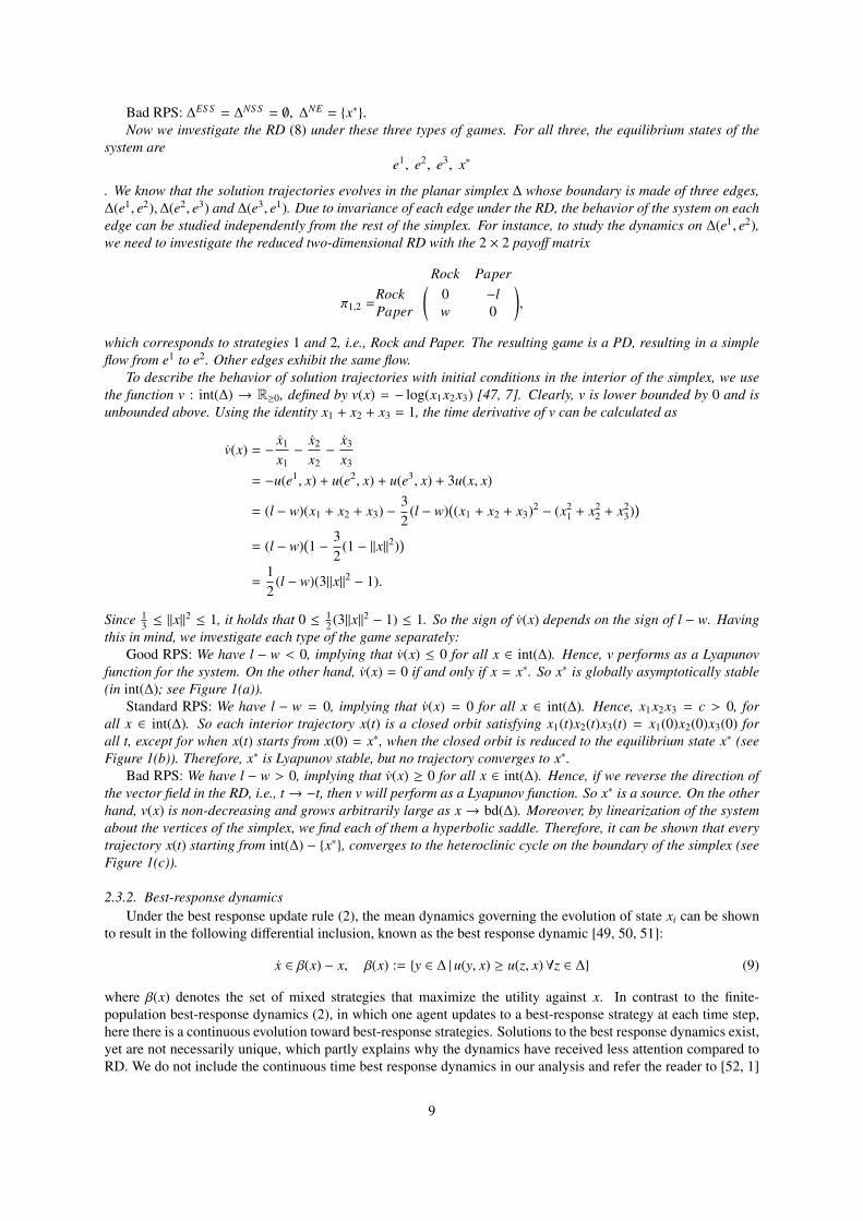
Bad RPS: ∆ES S = ∆NS S = ∅, ∆NE = x∗.Now we investigate the RD (8) under these three types of games. For all three, the equilibrium states of the

system aree1, e2, e3, x∗

. We know that the solution trajectories evolves in the planar simplex ∆ whose boundary is made of three edges,∆(e1, e2),∆(e2, e3) and ∆(e3, e1). Due to invariance of each edge under the RD, the behavior of the system on eachedge can be studied independently from the rest of the simplex. For instance, to study the dynamics on ∆(e1, e2),we need to investigate the reduced two-dimensional RD with the 2 × 2 payoff matrix

π1,2 =

( Rock PaperRock 0 −lPaper w 0

),

which corresponds to strategies 1 and 2, i.e., Rock and Paper. The resulting game is a PD, resulting in a simpleflow from e1 to e2. Other edges exhibit the same flow.

To describe the behavior of solution trajectories with initial conditions in the interior of the simplex, we usethe function v : int(∆) → R≥0, defined by v(x) = − log(x1x2x3) [47, 7]. Clearly, v is lower bounded by 0 and isunbounded above. Using the identity x1 + x2 + x3 = 1, the time derivative of v can be calculated as

v(x) = −x1

x1−

x2

x2−

x3

x3

= −u(e1, x) + u(e2, x) + u(e3, x) + 3u(x, x)

= (l − w)(x1 + x2 + x3) −32

(l − w)((x1 + x2 + x3)2 − (x2

1 + x22 + x2

3))

= (l − w)(1 −

32

(1 − ‖x‖2))

=12

(l − w)(3‖x‖2 − 1).

Since 13 ≤ ‖x‖

2 ≤ 1, it holds that 0 ≤ 12 (3‖x‖2 − 1) ≤ 1. So the sign of v(x) depends on the sign of l − w. Having

this in mind, we investigate each type of the game separately:Good RPS: We have l − w < 0, implying that v(x) ≤ 0 for all x ∈ int(∆). Hence, v performs as a Lyapunov

function for the system. On the other hand, v(x) = 0 if and only if x = x∗. So x∗ is globally asymptotically stable(in int(∆); see Figure 1(a)).

Standard RPS: We have l − w = 0, implying that v(x) = 0 for all x ∈ int(∆). Hence, x1x2x3 = c > 0, forall x ∈ int(∆). So each interior trajectory x(t) is a closed orbit satisfying x1(t)x2(t)x3(t) = x1(0)x2(0)x3(0) forall t, except for when x(t) starts from x(0) = x∗, when the closed orbit is reduced to the equilibrium state x∗ (seeFigure 1(b)). Therefore, x∗ is Lyapunov stable, but no trajectory converges to x∗.

Bad RPS: We have l − w > 0, implying that v(x) ≥ 0 for all x ∈ int(∆). Hence, if we reverse the direction ofthe vector field in the RD, i.e., t → −t, then v will perform as a Lyapunov function. So x∗ is a source. On the otherhand, v(x) is non-decreasing and grows arbitrarily large as x → bd(∆). Moreover, by linearization of the systemabout the vertices of the simplex, we find each of them a hyperbolic saddle. Therefore, it can be shown that everytrajectory x(t) starting from int(∆) − x∗, converges to the heteroclinic cycle on the boundary of the simplex (seeFigure 1(c)).

2.3.2. Best-response dynamicsUnder the best response update rule (2), the mean dynamics governing the evolution of state xi can be shown

to result in the following differential inclusion, known as the best response dynamic [49, 50, 51]:

x ∈ β(x) − x, β(x) := y ∈ ∆ | u(y, x) ≥ u(z, x)∀z ∈ ∆ (9)

where β(x) denotes the set of mixed strategies that maximize the utility against x. In contrast to the finite-population best-response dynamics (2), in which one agent updates to a best-response strategy at each time step,here there is a continuous evolution toward best-response strategies. Solutions to the best response dynamics exist,yet are not necessarily unique, which partly explains why the dynamics have received less attention compared toRD. We do not include the continuous time best response dynamics in our analysis and refer the reader to [52, 1]

9

(a) (b) (c)

Figure 1: Flow patterns of the Replicator Dynamics for the good, standard and bad Rock-Paper-Scissors (RPS) games. The plots indicatethe evolution of the solution trajectory x(t) for some initial conditions on the simplex ∆. Color temperatures are used to show motion speeds,where red corresponds to the fastest and blue to the slowest motion. The circles denote equilibria. For all three types of games, the dynamicsadmit three boundary equilibrium points, e1, e2 and e3, which are the vertices of the simplex, and a unique interior equilibrium x∗ in the middleof the simplex. (a) good RPS: x∗ is globally asymptotically stable in the interior of the simplex. (b) standard RPS: x∗ is Lyapunov stable, andall orbits in the interior of the simplex are closed orbits, encircling x∗. (c) bad RPS: x∗ is a source, and all orbits in the interior of the simplexconverge to the heteroclinic cycle formed by the boundary of the simplex. The figures are produced using the software Dynamo [48].

for more information. In the rest of the paper, by “best response dynamics”, rather than (9), we simply mean thediscrete dynamics caused by the best response update rule.

3. Equilibrium convergence and stability

3.1. Infinite well-mixed populations (continuous-time continuous-state dynamics)

General stability and convergence results for continuous dynamics such as the Poincare-Bendixson theoremcan, of course, be used for RD whenever applicable [53, 43]. However, interestingly enough, convergence, andparticularly, stability notions such as Lyapunov stability for RD, are tightly linked to game theoretical notionssuch as Nash equilibrium. The first are notions defined for vector fields and dynamical systems whereas thesecond are defined in the absence of any dynamic. This enables us to make conclusions on the evolution of thesolution trajectories of RD through game-theoretic analyses of the corresponding payoff matrix. In what follows,we review some well-known results that reveal these links. The reader may consult any of the books [54, 7, 1] formore details.

3.1.1. Equilibrium statesBy letting the right-hand side of (8) equal to zero, we get the condition u(ei, x) = u(x, x) or xi = 0 for all i ∈ S,

for x to be an equilibrium. This is closely related to the definition of a Nash strategy, as revealed by the followingproposition [7]. Let ∆o denote the set of equilibrium states of (8).

Proposition 1. The following holds

• ∆NE ∪ e1, . . . , em ⊆ ∆o;

• int(∆o) = ∆NE ∩ int(∆);

• int(∆o) is convex.

In addition to the trivial result that every vertex of the simplex is an equilibrium, the first statement impliesthat every Nash strategy is also an equilibrium of RD. Namely, if a strategy is the best-response to itself, thecorresponding population state is an equilibrium of RD. The reverse, however, does not hold. Yet the secondstatement clarifies that only a non-interior equilibrium state may not be a Nash strategy. That is, all interiorequilibria are a Nash strategy. The last statement postulates the convexity of the set of interior equilibria, implyingthat it can be a singleton, straight line, plane, etc. in the simplex, but it cannot be two disjoint points, for example.

10

3.1.2. Lyapunov stable statesThe role of Nash strategies is not limited to equilibrium states. The following result states that every stable

state in (8) has to be a Nash strategy [55].

Proposition 2. If x∗ ∈ ∆ is Lyapunov stable in (8), then x∗ ∈ ∆NE .

As an application of the Proposition, the equilibrium point x∗ in Example 1 is Lyapunov stable in the goodand standard RPS games, and indeed is neutrally stable in both cases. Intuitively, Proposition 2 implies that onlypopulation states whose corresponding strategy vector performs best against itself can be stable under RD. Thisnecessary condition is not sufficient though; a simple example is RD for the 2 × 2 coordination game where themixed strategy is a Nash strategy but is unstable (see “Analyses of the replicator dynamics for 2x2 games”). Thefollowing result provides a sufficient stability condition [7].

Proposition 3. Every x∗ ∈ ∆NS S is Lyapunov stable in (8).

Again back to Example 1, x∗ is neutrally stable in the good and standard RPS games, and is also Lyapunovstable in both cases. According to Proposition 3, if strategy x∗ performs at least as well as any group of mutantsarising in a population of all x∗-players, provided that the mutant population is small enough, then under RD, thesolution trajectory remains in a small neighborhood of the population state x∗, if it starts sufficiently close to x∗.The reverse, however, does not hold as discussed in Example 2.

3.1.3. Asymptotically stable statesClearly, in view of Proposition 2, every asymptotically stable state has to be a Nash strategy, yet this strong

notion of stability further confines the Nash strategy to a perfect Nash strategy [55].

Proposition 4. If x∗ ∈ ∆ is asymptotically stable in (8), then x∗ ∈ ∆PNE .

So if every close-by trajectory to the population state x∗, not only remains close, but also converges to x∗, thenx∗ must be a Nash strategy that is robust against some ‘trembles’ in the player’s strategy. The necessary conditionin Proposition 4 is not sufficient though. For instance, x∗ in Example 1 is perfect since it belongs to the interior ofthe simplex, yet it is unstable in the bad RPS game.

Now we proceed to the most well-known result for RD, providing a sufficient condition for asymptotic stabilityby bridging this notion to that of evolutionary stability [37, 56].

Proposition 5. Every x∗ ∈ ∆ES S is asymptotically stable in (8).

Back to Example 1, x∗ is evolutionarily stable in the good RPS game and is also asymptotically stable. Notethat according to the proposition, strict Nash strategies which are Nash strategies that satisfy (B.1) with strict in-equality, are also asymptotically stable since they are an ESS. Intuitively, this condition is not necessary for asymp-totic stability: evolutionary stability requires x∗ to outperform any sufficiently small group of mutants against theresulting population mixture, yet for asymptotic stability of x∗, it is possible to do worse than some mutant typey ∈ ∆, provided that there is some other mutant z ∈ ∆ that outperforms y, but does worse against x∗. This isillustrated in the following example.

Example 2. Consider a symmetric two-player game with the payoff matrix

π =

0 6 −4−3 0 5−1 3 0

.The game is often referred to as Zeeman’s game, named after Zeeman [57, 1]. We study the game under the RD.The equilibrium points and their local stability are as follows: five equilibrium points on bd(∆): e1: hyperbolicstable, e2: hyperbolic unstable, e3: hyperbolic saddle, x23 =

[0 5

838

]>, located on the edge ∆(e2, e3): hyper-

bolic saddle, and x13 =[

45 0 1

5

]>, located on the edge ∆(e1, e3): hyperbolic saddle, and one equilibrium point

in int(∆): x∗ =[

13

13

13

]>: hyperbolic stable. So e1 and x∗ are asymptotically stable. Indeed, it can be shown

that for every initial condition in int(∆) except for those located on the stable manifold of x13 which connects e2

to x13, the solution trajectory converges to either e1 or x∗ (see Figure 2).

11

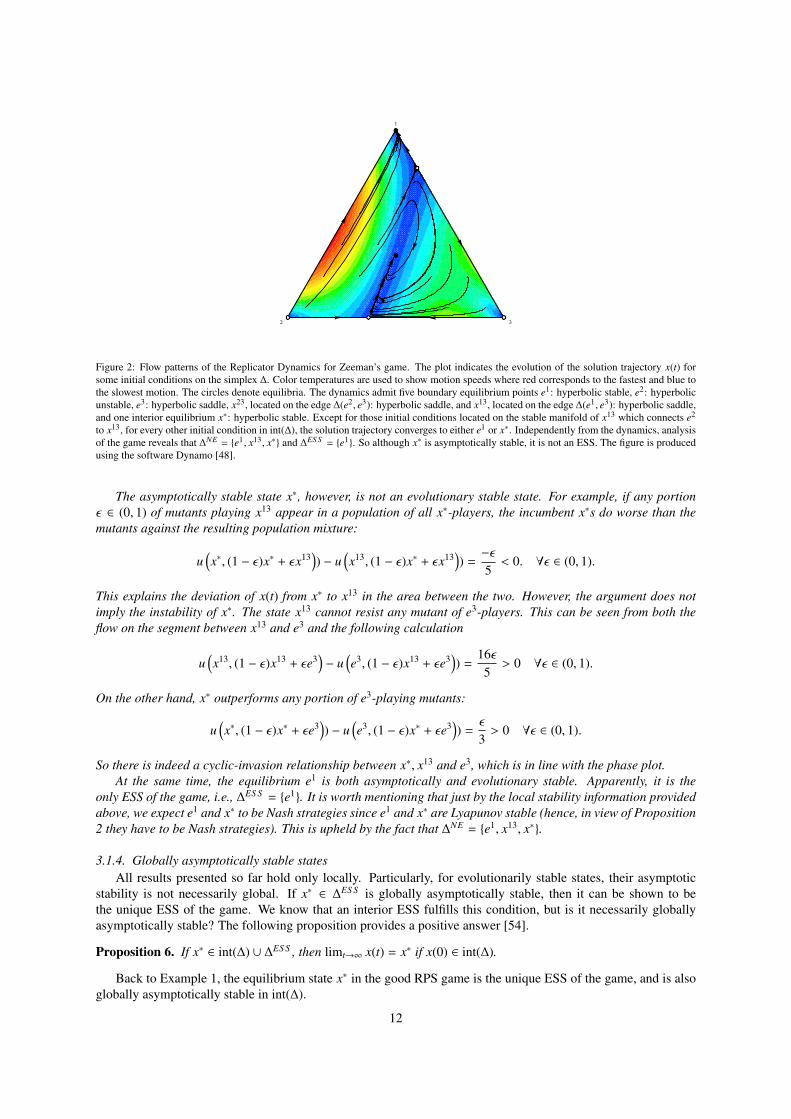
1

2 3

Figure 2: Flow patterns of the Replicator Dynamics for Zeeman’s game. The plot indicates the evolution of the solution trajectory x(t) forsome initial conditions on the simplex ∆. Color temperatures are used to show motion speeds where red corresponds to the fastest and blue tothe slowest motion. The circles denote equilibria. The dynamics admit five boundary equilibrium points e1: hyperbolic stable, e2: hyperbolicunstable, e3: hyperbolic saddle, x23, located on the edge ∆(e2, e3): hyperbolic saddle, and x13, located on the edge ∆(e1, e3): hyperbolic saddle,and one interior equilibrium x∗: hyperbolic stable. Except for those initial conditions located on the stable manifold of x13 which connects e2

to x13, for every other initial condition in int(∆), the solution trajectory converges to either e1 or x∗. Independently from the dynamics, analysisof the game reveals that ∆NE = e1, x13, x∗ and ∆ES S = e1. So although x∗ is asymptotically stable, it is not an ESS. The figure is producedusing the software Dynamo [48].

The asymptotically stable state x∗, however, is not an evolutionary stable state. For example, if any portionε ∈ (0, 1) of mutants playing x13 appear in a population of all x∗-players, the incumbent x∗s do worse than themutants against the resulting population mixture:

u(x∗, (1 − ε)x∗ + εx13

)) − u

(x13, (1 − ε)x∗ + εx13

)) =−ε

5< 0. ∀ε ∈ (0, 1).

This explains the deviation of x(t) from x∗ to x13 in the area between the two. However, the argument does notimply the instability of x∗. The state x13 cannot resist any mutant of e3-players. This can be seen from both theflow on the segment between x13 and e3 and the following calculation

u(x13, (1 − ε)x13 + εe3

)− u

(e3, (1 − ε)x13 + εe3

)) =

16ε5

> 0 ∀ε ∈ (0, 1).

On the other hand, x∗ outperforms any portion of e3-playing mutants:

u(x∗, (1 − ε)x∗ + εe3

)) − u

(e3, (1 − ε)x∗ + εe3

)) =

ε

3> 0 ∀ε ∈ (0, 1).

So there is indeed a cyclic-invasion relationship between x∗, x13 and e3, which is in line with the phase plot.At the same time, the equilibrium e1 is both asymptotically and evolutionary stable. Apparently, it is the

only ESS of the game, i.e., ∆ES S = e1. It is worth mentioning that just by the local stability information providedabove, we expect e1 and x∗ to be Nash strategies since e1 and x∗ are Lyapunov stable (hence, in view of Proposition2 they have to be Nash strategies). This is upheld by the fact that ∆NE = e1, x13, x∗.

3.1.4. Globally asymptotically stable statesAll results presented so far hold only locally. Particularly, for evolutionarily stable states, their asymptotic

stability is not necessarily global. If x∗ ∈ ∆ES S is globally asymptotically stable, then it can be shown to bethe unique ESS of the game. We know that an interior ESS fulfills this condition, but is it necessarily globallyasymptotically stable? The following proposition provides a positive answer [54].

Proposition 6. If x∗ ∈ int(∆) ∪ ∆ES S , then limt→∞ x(t) = x∗ if x(0) ∈ int(∆).

Back to Example 1, the equilibrium state x∗ in the good RPS game is the unique ESS of the game, and is alsoglobally asymptotically stable in int(∆).

12

3.1.5. Convergence resultsAs with most other dynamics, existing stability results on RD are insufficient to describe the global behavior

of the trajectories. Local stability analysis illustrates the flow only in the neighborhood of the equilibria, andglobal ones, such as global stability, rarely take place in these dynamics. One fundamental question on the globalbehavior of the dynamics is under what conditions every solution trajectory converges to an equilibrium point?Symmetry of the payoff matrix turns out to guarantee this. The average fitness in doubly symmetric games, thoseare symmetric games with a symmetric payoff matrix, is non-decreasing over time, i.e., u(x, x) ≥ 0 with equalityif and only if x is an equilibrium point. This can be considered as a version of the Fundamental Theorem ofNatural Selection [58] stated in a more general context at 1930, before the invention of RD: The rate of increasein fitness of any organism at any time is equal to its genetic variance in fitness at that time. However, this does notprove equilibrium convergence, and by using theorems such as LaSalle’s invariance principle, we can only showconvergence to the set of equilibrium states in RD. Yet it was later shown in [59] that symmetry of the payoff

matrix is indeed sufficient for equilibrium convergence.

Proposition 7. If the game is doubly symmetric, i.e., π = π>, then every trajectory converges to an equilibriumpoint.

Often the payoff matrix is not symmetric, yet is symmetrizable by local shifts, that is the addition of a constantto every entry of a column, captured by the transformation T : Rm×m → Rm×m defined as T (π) = π + 1c>

where 1 is the all-one and c is a constant vector, both in Rm×1. The RD are invariant under local shifts [7].Therefore, Proposition 7 also holds for any game with a symmetrizable payoff matrix. For example, all symmetric2 × 2 games admit equilibrium convergence under RD. Some games, however, are neither doubly symmetric norsymmetrizable, yet exhibit equilibrium convergence, such as the good RPS game in Example 1.

Now given the convergence of RD for a particular payoff matrix, the next natural question is to what kind ofequilibrium point the trajectory may converge. Apparently if the trajectory starts from some interior point of thesimplex, the final stationary state has to be the best response to itself [60].

Proposition 8. If x(0) ∈ int(∆) and limt→∞ x(t) = x∗, then x∗ ∈ ∆NE .

Visiting back Example 2, based on the dynamics, we expect x13 ∈ ∆NE since at least one interior trajectoryconverges to x13, which is the one on the stable manifold of x13. The role of a Nash strategy is not limited toProposition 8 though. If the interior of the simplex is empty of Nash strategies, or equivalently empty of anyequilibrium point (see Proposition 1), then every trajectory converges to the boundary of the simplex [61].

Proposition 9. If int(∆) ∩ ∆NE = ∅, then x(t)→ bd(∆) as t → ∞.

So it is impossible for the trajectories to meander forever in the interior of an empty-equilibrium simplex.

3.1.6. Folk TheoremBy summarizing some of the results we presented so far on the relation of Nash strategies and RD, we arrive

at the following theorem [62, 63].

Theorem 1 (Folk Theorem of Evolutionary Game Theory). The RD (8) satisfy the following statements:

1. A Lyapunov stable equilibrium is a Nash strategy;2. If a solution trajectory starting from the interior of the simplex converges to a point, that point has to be a

Nash strategy;3. A strict Nash strategy is locally asymptotically stable.

The results of the theorem are known to be a paradigm shift towards strategic reasoning: The Folk Theoremmeans that biologists can predict the evolutionary outcome of their stable systems by examining behavior of theunderlying game [62]. However, the theorem does not hold for every other type of dynamics such as the monotoneselection dynamics [62, 7].

13

3.2. Infinite structured populations (continuous-time continuous-state dynamics)Before returning to the case of finite populations, we briefly discuss some results for infinite populations in

which the well-mixed assumption is relaxed. That is, individuals of a given type (strategy) may interact withother types of individuals in different proportions. These interactions can be modeled by a graph in which thenodes represent the available strategies and the connections are weighted according to the interaction probabilitiesbetween each strategy pair. The corresponding mean dynamics can then be expressed while taking these interac-tion probabilities into account [64]. Some important properties such as stability of Nash equilibria are preservedunder this modification for various dynamics, even when individuals playing particular strategies do not have fullinformation about the utilities associated with other strategies [65].

3.3. Finite structured populations (discrete-time discrete-state dynamics)We now turn back to the general case of discrete-time dynamics on finite networks, for which both the notion

of convergence and the tools needed for its analysis differ substantially from the continuous case. In continuousdynamics, convergence of a solution trajectory x(t) to an equilibrium point x∗ implies that the distance from thetrajectory to the equilibrium, i.e., ‖x(t) − x∗‖, becomes arbitrary small, yet never necessarily zero, as time goes toinfinity. On the other hand, discrete population dynamics take place over a discrete time sequence k = 0, 1, 2, . . .and the state of system is a discrete vector x ∈ Sn. Therefore, notions such as ‘arbitrary small yet nonzero’are undefinable for the distance from the trajectory to an equilibrium, because ‖x(k) − x∗‖ takes discrete values0, 1, 2, . . .. Instead, we have the notion of ‘reaching’ an equilibrium state, that is, when x(k) exactly equals x∗.This highlights a key difference from convergence in continuous dynamics, which is that the state x(k) becomesfixed at x∗ at some finite time T and does not change afterwards, whereas convergence in continuous dynamicstypically never leads to the state reaching an equilibrium in finite time. Despite the differences, ‘convergence’ isoften used for both continuous and discrete dynamics, a convention that we also adopt in this paper. However, itshould be clear to the reader that the study of equilibrium convergence for discrete population dynamics can beinterpreted as the investigation of whether solution trajectories reach equilibrium states.

As discussed in Section 3.1, continuous best-response and especially imitation dynamics can exhibit non-convergence and chaotic asymptotic behaviors, even under the simplifying assumptions of infinite and well-mixedpopulations. No less complex outcomes are therefore to be expected for finite structured populations governedby the discrete forms of these dynamics. Indeed, populations of just two (resp. three) agents can lead to non-convergence in discrete best-response (resp. imitation) dynamics. Hence, it becomes a challenging problem toidentify conditions under which a network can be expected to converge to an equilibrium under imitation andbest-response update rules, which we investigate in this section.

Inspired by the convergence results for the continuous population-dynamics discussed in earlier sections, onemay try to find Lyapunov (energy) functions, which are strictly positive and decreasing at each time step, to proveequilibrium convergence in the discrete case. Although sometimes possible, one should note that finding energy-like functions, which decrease at some time instances but remain constant at others, may be easier to constructand often the only choice. For example, in the discrete population-dynamics, a common phenomenon is an activeagent at time k not switching strategies, which keeps the state x(k + 1) the same as its value at the previous timeinstance x(k). Thus, the value of any candidate energy function remains the same at time k + 1, excluding it frombeing an strictly decreasing energy function, yet leaving room for being an energy-like function.

The number of agents updating at the same time, namely, the level of synchrony of the dynamics, turns outto greatly influence the asymptotic behavior of the population. For example, synchronous versions of the updaterules (2) and (6) are deterministic: there is exactly one possible state x2 to which the solution trajectory can transitfrom a given state x1, where x1 and x2 can be the same. Hence, the dynamics admit a unique ω-limit set in theform of a cycle of length at least 1, which is an equilibrium, and at most |S|n the number of possible states. Thechallenge then becomes determining the length of the limit cycle. For partial and asynchronous updates; however,the transition to the next state from a given state is usually not unique and depends on the active agent, resultingin non-deterministic dynamics, capable of exhibiting chaotic fluctuations as well as perpetual cycles.

In order to guarantee convergence in the discrete case, we must assume that the activation sequence is persis-tent, that is, every agent i ∈ V becomes active infinitely many times as time goes to infinity. Formally, given anagent i ∈ V and any time k ∈ 0, 1, . . ., there is some finite future time k′ > k at which agent i is active. One caneasily check that without this assumption equilibrium convergence may never happen.

3.3.1. ImitationThe best-response strategy in a 2-player matrix game is the one corresponding to the maximum entry in the

column of the payoff matrix defined by the opponent’s strategy. It is therefore intuitive that convergence relieson the ordering of payoff values within each column (which determines whether the agents are coordinating or

14

anti-coordinating [13]). On the other hand, under the imitation rule, the payoffs of the opponent play a greaterrole. Consequently, under imitation, the ordering of payoff values within each row appears to be the key.

We call an agent i ∈ V an opponent-coordinating agent if each diagonal entry of her payoff matrix πi is greaterthan all off-diagonal elements in the same row, that is

πip,p > π

ip,q ∀p, q ∈ 1, . . . ,m, p , q. (10)

The following theorem establishes convergence when updates are fully asynchronous [66, 43].

Theorem 2. Every network of opponent-coordinating agents reaches an equilibrium under the asynchronous im-itation update rule.

However, in order to guarantee convergence under synchronous and partially synchronous updates, the agentsmust satisfy a stronger condition than being opponent-coordinating. In other words, their payoff matrices mustsatisfy

πip,p + (degi −1)πi

p,pmin> degi π

ip,pmax

(11)

where degi denotes the degree of agent i, pmin denotes the column of the minimum off-diagonal entry of the pthrow in πi and pmax denotes the column of the maximum off-diagonal entry of the pth row in πi.

Then we can assert the following result, regardless of how many agents update simultaneously [66].

Theorem 3. Every network of strongly-opponent-coordinating agents reaches an equilibrium under the imitationupdate rule.

For the special case of m = 2, an opponent-coordinating agent turns out to be also strongly opponent-coordinating, implying that Theorem 2 holds even for partially synchronous dynamics.

3.3.2. Best-responseWhile there is no guarantee that a network of agents using best response updates (2) will reach an equilibrium

state in general, we present here three conditions on 2 × 2 payoff matrices for which convergence is assuredwhen updates are persistent and asynchronous: (i) when all agents are coordinating, (ii) when all agents are anti-coordinating, and (iii) when all games are symmetric. We refer the reader to Appendix G for proofs of thefollowing results using potential functions.

When all agents in the network are coordinating (see Section 2.2.1), we have the following theorem [13].

Theorem 4. Every network of coordinating agents who update asynchronously and persistently will reach anequilibrium state.

The following corollary follows directly from Theorem 4.

Corollary 1. Every network of coordinating agents admits a pure strategy Nash equilibrium.

The case of all anti-coordinating agents is perhaps a more surprising result, but convergence is indeed guaran-teed here as well [13].

Theorem 5. Every network of anti-coordinating agents who update asynchronously and persistently will reachan equilibrium state.

The following corollary follows directly from Theorem 5.

Corollary 2. Every network of anti-coordinating agents admits a pure strategy Nash equilibrium.

Although we have mostly considered cases when the payoff matrix πi of an agent applies to all neighbors, thegeneral case allows for a different payoff matrix πi, j for each neighbor j. It turns out that such a network will reachequilibrium provided that all pairwise games are symmetric.

Theorem 6. Every network of agents in which all games are symmetric, i.e. πi, j = π j,i for all i, j ∈ E, whoupdate asynchronously and persistently will reach an equilibrium state.

The following corollary follows directly from Theorem 6.

Corollary 3. Every network of agents in which all games are symmetric admits a pure strategy Nash equilibrium.

15

Although these three conditions are sufficient to guarantee convergence in asynchronous networks of agentswho update with best-responses, if these conditions do not hold, it is quite easy to construct examples in whichthe agents will never reach an equilibrium state. One such example is a network in which updates are fullysynchronous may never reach an equilibrium state. Suppose that, in a network consisting of only two agents, bothagents are anti-coordinating, update synchronously, and start from the strategy state (A, A). The dynamics aretherefore deterministic, and the following state of the agents will evolve as follows:

(A, A)→ (B, B)→ (A, A),

resulting in a cycle of length 2. Now suppose that both agents are coordinating and they start from (A, B). Thiswill lead to the following deterministic sequence: (A, B)→ (B, A)→ (A, B), again resulting in a cycle of length 2.

The above examples prove that equilibrium convergence is no longer guaranteed if the agents update in fullsynchrony.

Finally, we consider the case of partial synchrony, in which multiple agents, but not always all, update at eachtime step. These results require the following assumption, since we need some notion of real time to study thiscase.

Assumption 1. The inter-activation times for each agent are drawn from mutually independent probability dis-tributions with support on R≥0.

Based on this, the following theorem establishes convergence in a probabilistic sense [13].

Theorem 7. Every network of all coordinating or all anti-coordinating agents who update with partially syn-chronous dynamics that satisfy Assumption 1 almost surely reaches an equilibrium state in finite time.

4. Control strategies

Even when populations of interacting agents converge to an equilibrium, it may be an undesirable one fromthe perspective of a global cost function or some measure of collective welfare. In these cases, and when a centralagency has the ability to influence the actions or perturb the dynamics of some of the agents, it is of great interest tounderstand how such influence can be efficiently used to improve global outcomes in the network. In this section,we investigate and compare several different approaches for doing this.

4.1. Infinite well-mixed populations

When the system of interest is defined on a sufficiently large and densely connected population, it may beuseful to devise control strategies based on mean dynamics such as RD. Suppose the goal is to drive the systemmodeled by RD to a particular population state x∗ ∈ ∆. One of the first things to consider is what the control inputshould be. Although there are multiple possible approaches, perhaps the most natural and least invasive controlinput is to alter the payoff functions for the available strategies. This can mean offering incentives by adding to theutility of desired strategies, or enforcing penalties by subtracting from the utility of undesired strategies. Whenviewed from the perspective of a regulating agency or government, these two options are sometimes consideredas subsidies and taxes [67]. This type of control input vi(t) can be incorporated into RD as follows:

xi = [u(ei, x) + vi − u(x, x)]xi.

Let D := i ∈ S : x∗i > 0 denote the set of desired strategies. It was proposed in [68] that a regulator, having afixed amount αn of available funds, could offer subsidies to agents using each desired strategy i ∈ D in the amountof vi = α

x∗ixi

, and vi = 0 for each i < D. The closed-loop dynamics for i ∈ D then become

xi =

[(u(ei, x) + α

x∗ixi

)− (u(x, x) + α)

]xi = [u(ei, x) − u(x, x)]xi + α(x∗i − xi). (12)

Notice that when adding α x∗ixi

to the utility of each pure strategy ei, the average utility becomes

∑i∈S

xi

(u(ei, x) + α

x∗ixi

)=

∑i∈S

xiu(ei, x) +∑i∈S

αx∗i = u(x, x) + α,

16

since both x, x∗ ∈ ∆. Also extended to the case of heterogeneous populations (multi-population games) [69], thisformulation has the property that equilibrium points of (12) are also equilibrium points of the original RD (8) forany α > 0. This allows for stabilization of existing equilibrium points of a system, but not for stabilization ofarbitrary setpoints x∗, which remains an open research problem.

Similar to this approach, but using logit choice dynamics (a stochastic or noisy version of the best-responseupdate rule), [70] proposed pricing schemes to encourage efficient choices on roadway networks. This line ofresearch has been extended to more general economic contexts in [71]. In a continuous-time network setting, [72]characterized the number of control nodes required to stabilize desired equilibrium states of a best-response-likeepidemic model on path and star networks.

Although beyond the scope of this article, the shifting of equilibrium points has been considered in the contextof stochastically stable equilibria of evolutionary snowdrift games [73]. Also in a systems and control setting,RD has been invoked to study task assignment among team members [74], virus spread control [75], extremum-seeking controllers [76] and direct reciprocity [77].

4.2. Finite structured populationsSome concepts related to the control of populations on networks may differ from those related to control of

conventional dynamical systems, including the replicator dynamics. For example, there are multiple ways to affectthe dynamics in a way that can be considered a control input, including:

• direct strategy control – in some cases, it may be possible to fix the strategies of some of the agents in thenetwork, with the hope that there will be a cascading effect that produces a desired global outcome;

• incentive-based control – perhaps a more practical input is to give additional payoff as a reward or subtractpayoff as a penalty for using particular strategies.

Though not an exhaustive list, since most of the existing literature falls within one of these categories, we willfocus our attention on these. The control objective may also take different forms. For example, there may be adesired end state in some cases, but in other cases, this might not be a realistic goal. Rather, the goal could be toguide the population as close as possible toward a desired state.

Since very few mechanisms have been proposed for feedback control of population dynamics, we focus pri-marily on open-loop methods. A practical and compelling use of feedback in these kinds of systems remains aninteresting outstanding problem.

4.2.1. Unique convergence for a class of coordinating agentsDynamics that are known to converge in the absence of control serve as a natural starting point for the design

of control policies that try to steer a network towards a desired equilibrium. A potential obstacle in the designof such policies is that, due to the random sequence of updates under asynchronous dynamics, convergence doesnot generally result in a unique equilibrium. This makes it much more difficult to predict the outcome of acontrol action in an open-loop setting. However, there is a very useful property of networks consisting only ofcoordinating agents, which is that, if some strategies are fixed to A, or if incentives are provided for playing A, notonly is convergence guaranteed, but the network will converge to a unique equilibrium.

Before introducing this result, we need the following definitions.

Definition 1. We say that agent i is coordinating in X if whenever the agent would update to strategy X ∈ S, itwould also do so if some neighbors currently not playing X were instead playing X, that is, if for all x, x′ ∈ Sn,

if x′j =

x j if j < Ni or x j = Xx j or X otherwise

,

then fi(x, ui) = X =⇒ fi(x′, ui) = X,

where ui : S × Sn−1 → R is the utility function for agent i.For the next two definitions, we consider a situation in which some payoff incentives are offered to the agents

in a network which is at equilibrium. Let (G, π,R) denote a network game in which an equilibrium x∗ exists, andlet π denote a modification of the payoff matrix π such that for all Y,Z ∈ S

πiY,Z =

πiY,Z + ri if Y = Xπi

Y,Z otherwise

17

for all i ∈ V, where each ri ∈ R≥0.

Definition 2. We say that a network game is monotone in X if whenever some non-negative value is added tothe row corresponding to strategy X in the payoff matrices of some agents, when the network is currently at anequilibrium state, no agent will switch from X to some other strategy. That is, if x(k) = x∗, then under the networkgame (G, π,R),

xi(k) = X =⇒ xi(k + t) = X, for all i ∈ V and t ≥ k.

Definition 3. We say that a network game is uniquely convergent in X if whenever some non-negative value isadded to the row corresponding to strategy X in the payoff matrices of some agents, the network converges toa unique equilibrium state. Namely, when starting from x∗, the network game (G, π,R) converges to a uniqueequilibrium x regardless of the sequence in which the agents update their strategies.

We are now ready to state an important convergence result for networks of coordinating agents [78].

Theorem 8. Every network that is coordinating in strategy X is both monotone and uniquely convergent in X.

We can relate this result to best-response and imitation dynamics with the following corollaries [78].

Corollary 4. Every network consisting of all coordinating agents under two-strategy best-response dynamics iscoordinating in X for all X ∈ S.

Proof. According to the best-response rule (2), a coordinating agent will switch to a strategy X if a sufficientnumber of neighbors are currently playing X. It is therefore trivially true that if more agents in the network areplaying X, the agent will still update to X.

The following corollary provides a similar result for opponent-coordinating agents under imitation dynamics [78].

Corollary 5. Every network consisting of all opponent-coordinating agents under imitation dynamics is coordi-nating in X for all X ∈ S.

4.2.2. Direct strategy controlSuppose that by some means it is possible to fix the strategies of a subset L ⊆ V of the agents in a network:

xi(k + 1) =

x∗i , i ∈ Lfi(·), otherwise

, (13)

where x∗i denotes the strategy to fix for each control agent i ∈ L. In this case, it may be useful to know theminimum number of control agents necessary to drive the population to a desired equilibrium state.

Problem 1. Given a network game (G, π, f ) and initial state x(0), find the smallest set of control agents L∗ ⊆ Vand corresponding reference state x∗ such that the network will converge to the desired equilibrium state.

This problem is computationally complex to solve in general. However, some special network topologies admitexact analytical solutions for certain cases. For example, the results shown in Table 1 hold for two-strategy gameson completely connected networks of homogeneous imitating agents when x(0) = B and x∗ = A [42], whichdepend on the values of δB = d − b and δA = a − c.

Similar results exist for star and ring networks under the same assumptions[42]. For tree networks, it ispossible to bound and approximate the solution to this case of Problem 1 using an algorithm that traverses the treestructure from leaves to root [79]. A modification of this algorithm based on minimum spanning trees can also beused to approximate the solution on arbitrary networks for both deterministic and stochastic imitation dynamics[80, 42]. It has also been shown in a simulation study that controlling agents with higher degree results in ahigher frequency of cooperation than randomly controlling agents in a prisoner’s dilemma game under imitativedynamics on scale-free networks [41].

An alternative framework was presented in [81] for the direct-strategy control of synchronous networkedevolutionary games using large-scale logical dynamic networks to model transitions between all possible strategystates for various update rules. Equivalent conditions for reachability and stability are given in this work for aparticular set of control nodes. Using this general framework, a method was proposed in [82] for how to guide a

18

Table 1: Minimum number of direct control agents for to guide a network of completely connected agents who are playing strategy A to allplay strategy B.

δA + δB > 0 |L∗| =

min(⌊

1 + δB

δA+δB

⌋, n

), if δB ≥ 0

1, if δB < 0

δA + δB = 0 |L∗| =

n, if δB ≥ 01, if δB < 0

δA + δB < 0 |L∗| =

n, if δA ≥ 0 or

δB

δA+δB < n and (δA + δB) mod δB = 01, otherwise

network using best-response updates to an optimal state by adding a new player whose strategy can be controlleddirectly. Similarly in [83], the deterministic network dynamics were controlled by actively assigning the strategiesof a group of agents. However, since the underlying logical matrices have dimension mn, this line of analysis canbe intractable for large networks.

4.2.3. Incentive-based controlOne potentially effective policy-based control mechanism is to offer incentives to agents for playing a particular

strategy. Similar to the approach in Section 4.1, but in a discrete time setting, this is equivalent to adding somepositive value to the row in a payoff matrix corresponding to the desired strategy X:

πiX,Y := πi

X,Y + r for all Y ∈ S.

Although this approach is most intuitive for use with best-response dynamics, it can be applied to networks ofimitating agents as well. In the latter case, adding to the payoffs of an agent does not act as an “incentive” in thatit does not directly affect the decision of that agent. Rather, neighbors of the agent notice that agents who playthe rewarded strategy earn more total payoff and are therefore more likely to imitate them. We consider two casesunder this framework: (i) uniform rewards, when the same reward is offered to all agents in the network, and (ii)targeted rewards, when different rewards can be offered to different agents.

Uniform incentive-based control. In this case, the same incentive r0 is offered to every agent in the network:

πiX,Y := πi

X,Y + r0 for all i ∈ V and Y ∈ S.

Problem 2. Given initial equilibrium state x∗, find the minimum value of r0 such that the network will convergeto the equilibrium in which all agents play X.

It turns out that this problem can be solved exactly and efficiently provided that a network is both monotoneand uniquely convergent in the desired strategy, which holds for both best response and imitation dynamics. Inboth cases, the solution involves computing a set of all candidate rewards and then performing a binary searchover this finite set.

For networks of coordinating agents using best-response updates, the candidate set is given by:

RI :=

r ≥ γmax

∣∣∣∣ r =δi(nA

i − j)degi

, i ∈ V, j ∈ 1, . . . , nAi

.

where

γmax =

maxi∈B

δBi B , ∅

0 B = ∅, δi := δA

i + δBi ,

and B = i | δi = 0, xi(0) = B denotes a set of stubborn agents whose unaltered threshold is such that no numberof A-playing neighbors would cause them to switch from B to A [78].

For networks of opponent-coordinating agents using imitation dynamics, since no agent will switch from A to

19

B, the possible payoffs of an agent i when playing A (resp. B) at any time step are contained in the sets

ΠAi :=

ai(nA

i + ωi) + bi(degi −nAi − ωi) : ωi ∈ Ωi

ΠB

i :=ci(nA

i + ωi) + di(degi −nAi − ωi) : ωi ∈ Ωi

,

where Ωi = 0, 1, . . . , degi −nAi .

Now consider an agent s who initially plays B and has a neighbor j whose strategy was either initially A orbecame A at some other time. In order for agent j to cause agent s to switch to A, the payoff of agent j must begreater than that of each B-playing agent (denoted by i) in the neighborhood of agent s. Therefore, the reward

given to agent j must be greater thanuB

i −uAj

deg jfor some uB

i ∈ ΠBi and uA

j ∈ ΠAj . This leads to the following set of all

candidate infimum rewards [84].

RB :=uB

i − uAj

deg j

∣∣∣∣uBi ∈ ΠB

i , uAj ∈ ΠA

j , j ∈ Ns, i ∈ Ns ∪ s, xi(0) = B, s ∈ V, xs(0) = B∪ 0.

For both imitation and best-response, we then sort the elements of RI or RB in increasing order and denote thisvector by vR. Algorithm 1 then performs a binary search over vR to find the infimum reward such that all agentsin the network will eventually play A. Denote by 1 the n-dimensional vector containing all ones. In what follows,we also denote by x the unique equilibrium resulting from a particular set of incentives being offered to a networkof A-coordinating agents starting from x.

i− := 1i+ := |R|while i+ − i− > 1 do

r∗0 := vRj , where j := d i−+i+2 e

Γ := (G, π, f )Simulate Γ from x(0) until equilibrium xif xi = A for all i ∈ V then

i+ := jelse

i− := jend

endAlgorithm 1: Binary search over candidate rewards to find the value of r∗0 that solves Problem 2 for imitativenetworks of opponent-coordinating agents (R := RI) and best-response networks of coordinating agents (R :=RB)

Exact solutions for cases other than coordination remain an open area for investigation, which is likely to bechallenging since the guarantee of unique convergence no longer holds.

Targeted incentive-based control. Now suppose that the policy makers have the ability to offer different incentivesto different agents in the network:

πiX,Y = πi

X,Y + ri for all i ∈ V and Y ∈ S.

Problem 3. Given initial equilibrium state x∗, find r := (r1, . . . , rn)T with minimum sum such that the networkwill converge to the equilibrium in which all agents play X.

Problem 4. Given initial equilibrium state x∗ and budget constraint ρ, find r := (r1, . . . , rn)T such that∑n

i=1 ri ≤ ρthat maximizes the number of agents who converge to X.

Solutions to these problems are more difficult to compute for general networks since the outcome of offeringrewards strongly depends on which agents are offered rewards. A useful quantity to know is how much reward isrequired to cause some agent in the network to switch to the desired strategy. We will denote this quantity by ri,which takes different values depending on the update rule. For networks of opponent-coordinating agents under

20

imitation dynamics, the infimum reward such that at least one B-playing neighbor will switch to A is

ri = maxj∈NB

i

maxk∈NB

j

uk(B, x) − ui(A, x), (14)

when the state of the network is x, where NBi := j ∈ Ni ∪ i : x j = B denotes the self-inclusive set of neighbors

of agent i who are playing B [84].For networks of coordinating agents using best-response updates, the minimum incentive that will cause an

agent to switch from B to A depends on the agent payoff matrices and degree in the network. In particular, thefollowing condition must be satisfied for some agent i:

δinAi (te) = (γi − ri) degi ⇒ ri = γi −

δinAi (te)

degi.

Problems 3 and 4 now reduce to determining which agents to offer rewards to and in what order. Some po-tentially effective heuristics include targeting those agents who cause the most subsequent switches to the desiredstrategy or those who require the smallest rewards. The following algorithm can be used to iteratively implementany such heuristic.

Initialize xi = xi(0) and ri = 0 for each i ∈ Vwhile ∃i ∈ V : xi , A and

∑i∈V

ri < ρ do

AB := i ∈ V : xi = A ∧ [∃ j ∈ Ni : x j = B] ∧ ri ≤ ρ −∑

i∈V ri

Choose an agent j ∈ AB

Let r j := r j + r j + ε

Γ := (G, π, f )Simulate Γ from x until new equilibrium x′

x := x′end

Algorithm 2: Generic iterative algorithm for computing a reward vector to approximate the maximum numberof agents who will play strategy A. Since r j represents an infimum, an arbitrarily small additional payoff ε isadded to ensure that the reward causes an agent to switch.

Here we propose a weighted ratio of the two factors mentioned above, which, when implemented in Algorithm2, we call Iterative Potential-to-Reward Optimization (IPRO). Consider the following simple potential function

Φ(x) =

n∑i=1

nAi (x), (15)

where nAi (x) denotes the number of neighbors of agent i who play strategy A in the state x. The ratio we wish to

iteratively maximize is the following:

j∗ = arg maxj∈AB

∆Φ(x)α

rβj, (16)

where ∆Φ(x) := Φ(x′)−Φ(x), and α, β ≥ 0 are free design parameters. Although generally suboptimal, simulationshave shown that the IPRO algorithm outperforms several other agent-targeting heuristics and performs quite closeto optimal for a range of conditions on the network topology and payoff matrices, both for imitation [84] andbest-response dynamics [78]. The approach also seems to be effective for networks containing anti-coordinatingagents [78], although care should be taken because there is no guarantee of unique convergence in that case.

5. Open Problems

We summarize here some outstanding research problems discussed in this survey as well as some additionalones, categorized by dynamical regime.

5.1. Infinite well-mixed populationsFor infinite well-mixed populations, completing the gap between game-theoretical concepts such as evolution-

ary stability and dynamical concepts such as asymptotic stability is in particularly high demand. With regard to

21

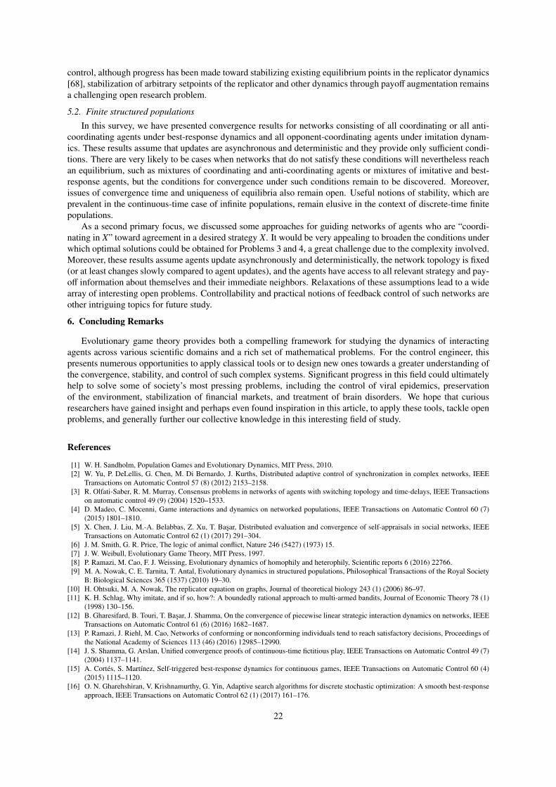
control, although progress has been made toward stabilizing existing equilibrium points in the replicator dynamics[68], stabilization of arbitrary setpoints of the replicator and other dynamics through payoff augmentation remainsa challenging open research problem.

5.2. Finite structured populations

In this survey, we have presented convergence results for networks consisting of all coordinating or all anti-coordinating agents under best-response dynamics and all opponent-coordinating agents under imitation dynam-ics. These results assume that updates are asynchronous and deterministic and they provide only sufficient condi-tions. There are very likely to be cases when networks that do not satisfy these conditions will nevertheless reachan equilibrium, such as mixtures of coordinating and anti-coordinating agents or mixtures of imitative and best-response agents, but the conditions for convergence under such conditions remain to be discovered. Moreover,issues of convergence time and uniqueness of equilibria also remain open. Useful notions of stability, which areprevalent in the continuous-time case of infinite populations, remain elusive in the context of discrete-time finitepopulations.

As a second primary focus, we discussed some approaches for guiding networks of agents who are “coordi-nating in X” toward agreement in a desired strategy X. It would be very appealing to broaden the conditions underwhich optimal solutions could be obtained for Problems 3 and 4, a great challenge due to the complexity involved.Moreover, these results assume agents update asynchronously and deterministically, the network topology is fixed(or at least changes slowly compared to agent updates), and the agents have access to all relevant strategy and pay-off information about themselves and their immediate neighbors. Relaxations of these assumptions lead to a widearray of interesting open problems. Controllability and practical notions of feedback control of such networks areother intriguing topics for future study.

6. Concluding Remarks

Evolutionary game theory provides both a compelling framework for studying the dynamics of interactingagents across various scientific domains and a rich set of mathematical problems. For the control engineer, thispresents numerous opportunities to apply classical tools or to design new ones towards a greater understanding ofthe convergence, stability, and control of such complex systems. Significant progress in this field could ultimatelyhelp to solve some of society’s most pressing problems, including the control of viral epidemics, preservationof the environment, stabilization of financial markets, and treatment of brain disorders. We hope that curiousresearchers have gained insight and perhaps even found inspiration in this article, to apply these tools, tackle openproblems, and generally further our collective knowledge in this interesting field of study.

References

[1] W. H. Sandholm, Population Games and Evolutionary Dynamics, MIT Press, 2010.[2] W. Yu, P. DeLellis, G. Chen, M. Di Bernardo, J. Kurths, Distributed adaptive control of synchronization in complex networks, IEEE

Transactions on Automatic Control 57 (8) (2012) 2153–2158.[3] R. Olfati-Saber, R. M. Murray, Consensus problems in networks of agents with switching topology and time-delays, IEEE Transactions

on automatic control 49 (9) (2004) 1520–1533.[4] D. Madeo, C. Mocenni, Game interactions and dynamics on networked populations, IEEE Transactions on Automatic Control 60 (7)

(2015) 1801–1810.[5] X. Chen, J. Liu, M.-A. Belabbas, Z. Xu, T. Basar, Distributed evaluation and convergence of self-appraisals in social networks, IEEE

Transactions on Automatic Control 62 (1) (2017) 291–304.[6] J. M. Smith, G. R. Price, The logic of animal conflict, Nature 246 (5427) (1973) 15.[7] J. W. Weibull, Evolutionary Game Theory, MIT Press, 1997.[8] P. Ramazi, M. Cao, F. J. Weissing, Evolutionary dynamics of homophily and heterophily, Scientific reports 6 (2016) 22766.[9] M. A. Nowak, C. E. Tarnita, T. Antal, Evolutionary dynamics in structured populations, Philosophical Transactions of the Royal Society

B: Biological Sciences 365 (1537) (2010) 19–30.[10] H. Ohtsuki, M. A. Nowak, The replicator equation on graphs, Journal of theoretical biology 243 (1) (2006) 86–97.[11] K. H. Schlag, Why imitate, and if so, how?: A boundedly rational approach to multi-armed bandits, Journal of Economic Theory 78 (1)

(1998) 130–156.[12] B. Gharesifard, B. Touri, T. Basar, J. Shamma, On the convergence of piecewise linear strategic interaction dynamics on networks, IEEE

Transactions on Automatic Control 61 (6) (2016) 1682–1687.[13] P. Ramazi, J. Riehl, M. Cao, Networks of conforming or nonconforming individuals tend to reach satisfactory decisions, Proceedings of

the National Academy of Sciences 113 (46) (2016) 12985–12990.[14] J. S. Shamma, G. Arslan, Unified convergence proofs of continuous-time fictitious play, IEEE Transactions on Automatic Control 49 (7)

(2004) 1137–1141.[15] A. Cortes, S. Martınez, Self-triggered best-response dynamics for continuous games, IEEE Transactions on Automatic Control 60 (4)

(2015) 1115–1120.[16] O. N. Gharehshiran, V. Krishnamurthy, G. Yin, Adaptive search algorithms for discrete stochastic optimization: A smooth best-response

approach, IEEE Transactions on Automatic Control 62 (1) (2017) 161–176.

22

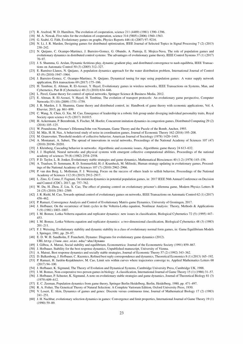
[17] R. Axelrod, W. D. Hamilton, The evolution of cooperation, science 211 (4489) (1981) 1390–1396.[18] M. A. Nowak, Five rules for the evolution of cooperation, science 314 (5805) (2006) 1560–1563.[19] G. Szabo, G. Fath, Evolutionary games on graphs, Physics Reports 446 (4) (2007) 97–9216.[20] N. Li, J. R. Marden, Designing games for distributed optimization, IEEE Journal of Selected Topics in Signal Processing 7 (2) (2013)

230–242.[21] N. Quijano, C. Ocampo-Martinez, J. Barreiro-Gomez, G. Obando, A. Pantoja, E. Mojica-Nava, The role of population games and

evolutionary dynamics in distributed control systems: The advantages of evolutionary game theory, IEEE Control Systems 37 (1) (2017)70–97.

[22] J. S. Shamma, G. Arslan, Dynamic fictitious play, dynamic gradient play, and distributed convergence to nash equilibria, IEEE Transac-tions on Automatic Control 50 (3) (2005) 312–327.

[23] E. Ramırez-Llanos, N. Quijano, A population dynamics approach for the water distribution problem, International Journal of Control83 (9) (2010) 1947–1964.

[24] J. Barreiro-Gomez, C. Ocampo-Martinez, N. Quijano, Dynamical tuning for mpc using population games: A water supply networkapplication, ISA transactions 69 (2017) 175–186.

[25] H. Tembine, E. Altman, R. El-Azouzi, Y. Hayel, Evolutionary games in wireless networks, IEEE Transactions on Systems, Man, andCybernetics, Part B (Cybernetics) 40 (3) (2010) 634–646.

[26] L. Pavel, Game theory for control of optical networks, Springer Science & Business Media, 2012.[27] E. Altman, R. El-Azouzi, Y. Hayel, H. Tembine, The evolution of transport protocols: An evolutionary game perspective, Computer

Networks 53 (10) (2009) 1751–1759.[28] J. R. Marden, J. S. Shamma, Game theory and distributed control, in: Handbook of game theory with economic applications, Vol. 4,

Elsevier, 2015, pp. 861–899.[29] C. Wang, X. Chen, G. Xie, M. Cao, Emergence of leadership in a robotic fish group under diverging individual personality traits, Royal

Society open science 4 (5) (2017) 161015.[30] H. Ackermann, P. Berenbrink, S. Fischer, M. Hoefer, Concurrent imitation dynamics in congestion games, Distributed Computing 29 (2)

(2016) 105–125.[31] W. Poundstone, Prisoner’s Dilemma/John von Neumann, Game Theory and the Puzzle of the Bomb, Anchor, 1993.[32] M. Mas, H. H. Nax, A behavioral study of noise in coordination games, Journal of Economic Theory 162 (2016) 195–208.[33] M. Granovetter, Threshold models of collective behavior, American Journal of Sociology (1978) 1420–1443.[34] A. Montanari, A. Saberi, The spread of innovations in social networks, Proceedings of the National Academy of Sciences 107 (47)

(2010) 20196–20201.[35] J. Kleinberg, Cascading behavior in networks: Algorithmic and economic issues, Algorithmic game theory 24 613–632.[36] J. J. Hopfield, Neural networks and physical systems with emergent collective computational abilities, Proceedings of the national

academy of sciences 79 (8) (1982) 2554–2558.[37] P. D. Taylor, L. B. Jonker, Evolutionary stable strategies and game dynamics, Mathematical Biosciences 40 (1-2) (1978) 145–156.[38] A. Traulsen, D. Semmann, R. D. Sommerfeld, H.-J. Krambeck, M. Milinski, Human strategy updating in evolutionary games, Proceed-

ings of the National Academy of Sciences 107 (7) (2010) 2962–2966.[39] P. van den Berg, L. Molleman, F. J. Weissing, Focus on the success of others leads to selfish behavior, Proceedings of the National

Academy of Sciences 112 (9) (2015) 2912–2917.[40] L. Zino, G. Como, F. Fagnani, On imitation dynamics in potential population games, in: 2017 IEEE 56th Annual Conference on Decision

and Control (CDC), 2017, pp. 757–762.[41] W. Du, H. Zhou, Z. Liu, X. Cao, The effect of pinning control on evolutionary prisoner’s dilemma game, Modern Physics Letters B

24 (25) (2010) 2581–2589.[42] J. R. Riehl, M. Cao, Towards optimal control of evolutionary games on networks, IEEE Transactions on Automatic Control 62 (1) (2017)

458–462.[43] P. Ramazi, Convergence Analysis and Control of Evolutionary Matrix-game Dynamics, University of Groningen, 2017.[44] J. Hofbauer, On the occurrence of limit cycles in the Volterra-Lotka equation, Nonlinear Analysis: Theory, Methods & Applications

5 (9) (1981) 1003–1007.[45] I. M. Bomze, Lotka-Volterra equation and replicator dynamics: new issues in classification, Biological Cybernetics 72 (5) (1995) 447–

453.[46] I. M. Bomze, Lotka-Volterra equation and replicator dynamics: a two-dimensional classification, Biological Cybernetics 48 (3) (1983)

201–211.[47] F. J. Weissing, Evolutionary stability and dynamic stability in a class of evolutionary normal form games, in: Game Equilibrium Models

I, Springer, 1991, pp. 29–97.[48] E. D. W. H. Sandholm, F. Franchetti, Dynamo: Diagrams for evolutionary game dynamics (2012).

URL http://www.ssc.wisc.edu/~whs/dynamo

[49] I. Gilboa, A. Matsui, Social stability and equilibrium, Econometrica: Journal of the Econometric Society (1991) 859–867.[50] J. Hofbauer, Stability for the best response dynamics, Unpublished manuscript, University of Vienna.[51] A. Matsui, Best response dynamics and socially stable strategies, Journal of Economic Theory 57 (2) (1992) 343–362.[52] D. Balkenborg, J. Hofbauer, C. Kuzmics, Refined best reply correspondence and dynamics, Theoretical Economics 8 (1) (2013) 165–192.[53] P. Ramazi, H. Jardon-Kojakhmetov, M. Cao, Limit sets within curves where trajectories converge to, Applied Mathematics Letters 68

(2017) 94–100.[54] J. Hofbauer, K. Sigmund, The Theory of Evolution and Dynamical Systems, Cambridge University Press, Cambridge UK, 1988.[55] I. M. Bomze, Non-cooperative two-person games in biology: A classification, International Journal of Game Theory 15 (1) (1986) 31–57.[56] J. Hofbauer, P. Schuster, K. Sigmund, A note on evolutionary stable strategies and game dynamics, Journal of Theoretical Biology 81 (3)

(1979) 609–612.[57] E. C. Zeeman, Population dynamics from game theory, Springer Berlin Heidelberg, Berlin, Heidelberg, 1980, pp. 471–497.[58] R. A. Fisher, The Genetical Theory of Natural Selection: A Complete Variorum Edition, Oxford University Press, 1930.[59] V. Losert, E. Akin, Dynamics of games and genes: Discrete versus continuous time, Journal of Mathematical Biology 17 (2) (1983)

241–251.[60] J. H. Nachbar, evolutionary selection dynamics in games: Convergence and limit properties, International Journal of Game Theory 19 (1)

(1990) 59–89.

23

[61] J. Hofbauer, A general cooperation theorem for hypercycles, Monatshefte fur Mathematik 91 (3) (1981) 233–240.[62] R. Cressman, Y. Tao, The replicator equation and other game dynamics, Proceedings of the National Academy of Sciences 111 (Supple-

ment 3) (2014) 10810–10817.[63] J. Hofbauer, K. Sigmund, Evolutionary game dynamics, Bulletin of the American Mathematical Society 40 (4) (2003) 479–519.[64] J. Barreiro-Gomez, G. Obando, N. Quijano, Distributed population dynamics: Optimization and control applications, IEEE Transactions

on Systems, Man, and Cybernetics: Systems 47 (2) (2017) 304–314.[65] A. Pantoja, N. Quijano, Distributed optimization using population dynamics with a local replicator equation, in: Decision and Control

(CDC), 2012 IEEE 51st Annual Conference on, IEEE, 2012, pp. 3790–3795.[66] P. Ramazi, J. Riehl, M. Cao, Imitating successful neighbors can hinder reaching satisfactory decisions for networks of decision-making

agents, under review.[67] T. Kanazawa, Y. Fukumoto, T. Ushio, T. Misaka, Replicator dynamics with pigovian subsidy and capitation tax, Nonlinear Analysis:

Theory, Methods & Applications 71 (12) (2009) e818–e826.[68] T. Kanazawa, T. Misaka, T. Ushio, Y. Fukumoto, A control method of selfish routing based on replicator dynamics with capitation tax

and subsidy, in: IEEE CCA & ISIC, 2009, pp. 249–254.[69] T. Morimoto, T. Kanazawa, T. Ushio, Subsidy-based control of heterogeneous multiagent systems modeled by replicator dynamics, IEEE

Transactions on Automatic Control 61 (10) (2016) 3158–3163.[70] W. H. Sandholm, Evolutionary implementation and congestion pricing, The Review of Economic Studies 69 (3) (2002) 667–689.[71] W. H. Sandholm, Pigouvian pricing and stochastic evolutionary implementation, Journal of Economic Theory 132 (1) (2007) 367–382.[72] A. Khanafer, T. Basar, B. Gharesifard, Stability properties of infected networks with low curing rates, in: American Control Conference

(ACC), 2014, IEEE, 2014, pp. 3579–3584.[73] H. Liang, M. Cao, X. Wang, Analysis and shifting of stochastically stable equilibria for evolutionary snowdrift games, Systems & Control

Letters 85 (2015) 16–22.[74] W. Mei, N. E. Friedkin, K. Lewis, F. Bullo, Dynamic models of appraisal networks explaining collective learning, IEEE Transactions on

Automatic Control.[75] E. Ramırez-Llanos, S. Martınez, A distributed dynamics for virus-spread control, Automatica 76 (2017) 41–48.[76] J. I. Poveda, N. Quijano, Shahshahani gradient-like extremum seeking, Automatica 58 (2015) 51–59.[77] P. Ramazi, M. Cao, Stability analysis for replicator dynamics of evolutionary snowdrift games, in: Decision and Control (CDC), 2014

IEEE 53rd Annual Conference on, IEEE, 2014, pp. 4515–4520.[78] J. Riehl, P. Ramazi, M. Cao, Control of asynchronous imitation dynamics on networks, arXiv preprint arXiv:1704.04416.[79] J. R. Riehl, M. Cao, Minimal-agent control of evolutionary games on tree networks, in: The 21st International Symposium on Mathe-

matical Theory of Networks and Systems, 2014.[80] J. R. Riehl, M. Cao, Control of stochastic evolutionary games on networks, IFAC-PapersOnLine 48 (22) (2015) 76–81.[81] D. Cheng, F. He, H. Qi, T. Xu, Modeling, analysis and control of networked evolutionary games, IEEE Transactions on Automatic

Control 60 (9) (2015) 2402–2415.[82] P. Guo, Y. Wang, H. Li, Algebraic formulation and strategy optimization for a class of evolutionary networked games via semi-tensor

product method, Automatica 49 (11) (2013) 3384–3389.[83] B. Zhu, X. Xia, Z. Wu, Evolutionary game theoretic demand-side management and control for a class of networked smart grid, Auto-

matica 70 (2016) 94–100.[84] J. Riehl, P. Ramazi, M. Cao, Control of asynchronous imitation dynamics on networks, arXiv preprint arXiv:1704.04416.[85] M. A. Nowak, Evolutionary Dynamics, Harvard University Press, 2006.

Appendix A. 2-player matrix games

A 2-player matrix game comprises two players, usually referred to as player 1 and player 2, two sets of purestrategies S1 = 1, . . . ,m1 and S2 = 1, . . . ,m2 from which players 1 and 2 choose strategies, and two payoff

matrices π1, π2 ∈ Rm1×m2 according to which players 1 and 2 earn payoffs, respectively. More specifically, whenplayer 1 plays strategy i ∈ S1 and player 2 plays strategy j ∈ S2, the payoff of the first and second players will beπ1

i j and π2ji, respectively. In this paper, we focus on matrix games that provide the same set of strategies for both

players, i.e., S = 1, 2, . . . ,m. The game is symmetric if π1 = π2.The players may be uncertain on their choices of strategies. For example, a player may choose strategy 1 with

probability 0.9 and strategy 2 with probability 0.1. This results in the so called mixed strategy which is defined asa vector x belonging to the simplex ∆ defined by

∆ :=

x ∈ Rm∣∣∣∣ ∑

i∈S

xi = 1, xi ≥ 0 ∀i ∈ S

.Namely, if a player plays the mixed strategy x, she will play each pure strategy i ∈ S with probability xi ∈ [0, 1],where

∑i∈S xi = 1. So if players 1 and 2 play the strategies x, y ∈ ∆, they will receive the payoffs u1(x, y) = x>π1y

and u2(y, x) = y>π2x, respectively, where ui : ∆ × ∆→ R, i ∈ 1, 2 are the utility functions of players 1 and 2. Tobe precise, one should distinguish the case when x equals a unit vector ei, i ∈ S, which is the ith column of them × m identity matrix, since then x refers to the pure strategy i. For this reason, the unit vector ei is called a purestrategy vector, which, with a minor abuse of notation, may also be referred to as the pure strategy i.

24

Appendix B. Nash equilibrium

Players’ strategies are said to be at a Nash equilibrium if no player would earn a higher payoff by changingtheir strategy. Particularly, for 2-player games, we have the following definition.

Definition 4. Consider a 2-player game with payoff matrices π1, π2 ∈ R2×2 and utility functions u1 and u2. A pairof strategies (x, y), where x, y ∈ ∆, is a Nash equilibrium if

u1(x, y) ≥ u1(z, y) ∀z ∈ ∆,

u2(y, x) ≥ u2(z, x) ∀z ∈ ∆.

A strict Nash equilibrium is a Nash equilibrium that satisfies both of the above conditions with strict inequality.For symmetric games, we further have the definition of a symmetric Nash equilibrium where the same strategy isplayed by both players. We call this same strategy, which is in Nash equilibrium with itself, a Nash strategy andformally define it as follows.

Definition 5. Consider a 2-player symmetric game with payoff matrix π and utility function u = u1 = u2, whereu(x, y) = x>πy for x, y ∈ ∆. A strategy x ∈ ∆ is a Nash strategy if

u(x, x) ≥ u(z, x) ∀z ∈ ∆. (B.1)

The set of all Nash strategies of the game is denoted by ∆NE .

A strict Nash strategy is a Nash strategy that satisfies (B.1) with strict inequality.Another refined definition of a Nash equilibrium is a perfect Nash equilibrium which is a Nash equilibrium

that is robust against some ‘trembles’ in the players’ strategies. Particularly, for symmetric games, we have thefollowing definition [7]. Consider a symmetric game G and an error vector µ ∈ ∆ where µi < 1 for i ∈ S. Definethe perturbed game G(µ) as the game G but when each pure strategy i ∈ S is played “by mistake” with probabilityµi by both players; namely, the strategies of both players belong to ∆(µ) = z ∈ ∆ | zi ≥ µi ∀i ∈ S. Denote by∆NE(µ) the set of Nash strategies of the perturbed game G(µ).

Definition 6. A strategy x ∈ ∆NE is a perfect Nash strategy if for some sequence G(µt)µt→0 of perturbed games,µt ∈ ∆, there exist Nash strategies xt ∈ ∆NE(µ) such that xt → x. The set of all perfect Nash strategies of the gameis denoted by ∆PNE .

It can be shown that every Nash strategy x belonging to the interior of the simplex ∆ is perfect.

Appendix C. Categorization of 2 × 2 matrix games

Symmetric matrix games in which both players have two strategies, typically referred to as cooperation (C)and defection (D), are widely studied in the context of evolutionary dynamics. These matrix games can be dividedinto the following four main categories based on the relationship between the payoffs in the matrix

π =

(C DC R SD T P

), R, S ,T, P ∈ R.

Prisoner’s Dilemma. In the prisoner’s dilemma game, described in Section 2, the payoffs must satisfy T > R andP > S . The state in which both players defect is a unique Nash equilibrium. In addition, it is usually requiredthat R > P to ensure that mutual cooperation is preferable to mutual defection. Otherwise, it is simply a game inwhich defection is the dominant strategy.

Anti-coordination, Snowdrift, Hawk-Dove, or Chicken. . In an anti-coordination game, players benefit when theyplay the same strategy as their opponents. In this case, the payoffs should satisfy T > R and S > P, and thereexist two pure strategy Nash Equilibria, which correspond to one player cooperating and the other defecting.Other versions of the game, such as snowdrift, are often considered less generic in the literature by enforcing theadditional requirement of R > S .

25

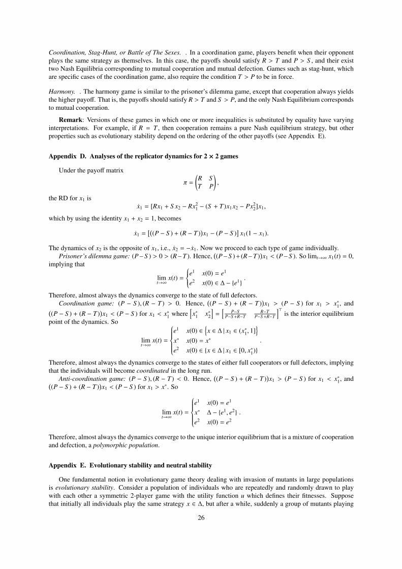
Coordination, Stag-Hunt, or Battle of The Sexes. . In a coordination game, players benefit when their opponentplays the same strategy as themselves. In this case, the payoffs should satisfy R > T and P > S , and their existtwo Nash Equilibria corresponding to mutual cooperation and mutual defection. Games such as stag-hunt, whichare specific cases of the coordination game, also require the condition T > P to be in force.

Harmony. . The harmony game is similar to the prisoner’s dilemma game, except that cooperation always yieldsthe higher payoff. That is, the payoffs should satisfy R > T and S > P, and the only Nash Equilibrium correspondsto mutual cooperation.

Remark: Versions of these games in which one or more inequalities is substituted by equality have varyinginterpretations. For example, if R = T , then cooperation remains a pure Nash equilibrium strategy, but otherproperties such as evolutionary stability depend on the ordering of the other payoffs (see Appendix E).

Appendix D. Analyses of the replicator dynamics for 2 × 2 games

Under the payoff matrix

π =

(R ST P

),

the RD for x1 isx1 = [Rx1 + S x2 − Rx2

1 − (S + T )x1x2 − Px22]x1,

which by using the identity x1 + x2 = 1, becomes

x1 =[(

(P − S ) + (R − T ))x1 − (P − S )

]x1(1 − x1).

The dynamics of x2 is the opposite of x1, i.e., x2 = −x1. Now we proceed to each type of game individually.Prisoner’s dilemma game: (P−S ) > 0 > (R−T ). Hence,

((P−S )+ (R−T )

)x1 < (P−S ). So limt→∞ x1(t) = 0,

implying that

limt→∞

x(t) =

e1 x(0) = e1

e2 x(0) ∈ ∆ − e1.

Therefore, almost always the dynamics converge to the state of full defectors.Coordination game: (P − S ), (R − T ) > 0. Hence,

((P − S ) + (R − T )

)x1 > (P − S ) for x1 > x∗1, and(

(P − S ) + (R − T ))x1 < (P − S ) for x1 < x∗1 where

[x∗1 x∗2

]=

[P−S

P−S +R−TR−T

P−S +R−T

]>is the interior equilibrium

point of the dynamics. So

limt→∞

x(t) =

e1 x(0) ∈

x ∈ ∆ | x1 ∈ (x∗1, 1]

x∗ x(0) = x∗

e2 x(0) ∈ x ∈ ∆ | x1 ∈ [0, x∗1).

Therefore, almost always the dynamics converge to the states of either full cooperators or full defectors, implyingthat the individuals will become coordinated in the long run.

Anti-coordination game: (P − S ), (R − T ) < 0. Hence,((P − S ) + (R − T )

)x1 > (P − S ) for x1 < x∗1, and(

(P − S ) + (R − T ))x1 < (P − S ) for x1 > x∗. So

limt→∞

x(t) =

e1 x(0) = e1

x∗ ∆ − e1, e2

e2 x(0) = e2

.

Therefore, almost always the dynamics converge to the unique interior equilibrium that is a mixture of cooperationand defection, a polymorphic population.

Appendix E. Evolutionary stability and neutral stability

One fundamental notion in evolutionary game theory dealing with invasion of mutants in large populationsis evolutionary stability. Consider a population of individuals who are repeatedly and randomly drawn to playwith each other a symmetric 2-player game with the utility function u which defines their fitnesses. Supposethat initially all individuals play the same strategy x ∈ ∆, but after a while, suddenly a group of mutants playing

26

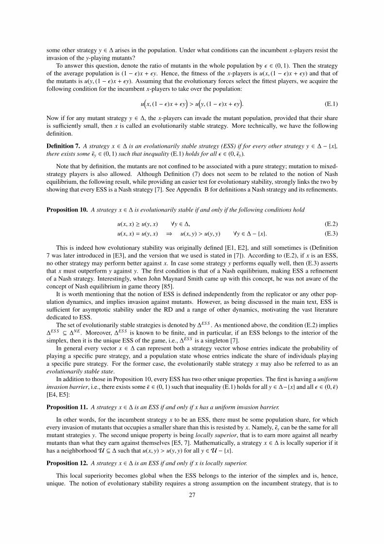
some other strategy y ∈ ∆ arises in the population. Under what conditions can the incumbent x-players resist theinvasion of the y-playing mutants?

To answer this question, denote the ratio of mutants in the whole population by ε ∈ (0, 1). Then the strategyof the average population is (1 − ε)x + εy. Hence, the fitness of the x-players is u(x, (1 − ε)x + εy) and that ofthe mutants is u(y, (1 − ε)x + εy). Assuming that the evolutionary forces select the fittest players, we acquire thefollowing condition for the incumbent x-players to take over the population:

u(x, (1 − ε)x + εy

)> u

(y, (1 − ε)x + εy

). (E.1)

Now if for any mutant strategy y ∈ ∆, the x-players can invade the mutant population, provided that their shareis sufficiently small, then x is called an evolutionarily stable strategy. More technically, we have the followingdefinition.

Definition 7. A strategy x ∈ ∆ is an evolutionarily stable strategy (ESS) if for every other strategy y ∈ ∆ − x,there exists some εy ∈ (0, 1) such that inequality (E.1) holds for all ε ∈ (0, εy).

Note that by definition, the mutants are not confined to be associated with a pure strategy; mutation to mixed-strategy players is also allowed. Although Definition (7) does not seem to be related to the notion of Nashequilibrium, the following result, while providing an easier test for evolutionary stability, strongly links the two byshowing that every ESS is a Nash strategy [7]. See Appendix B for definitions a Nash strategy and its refinements.

Proposition 10. A strategy x ∈ ∆ is evolutionarily stable if and only if the following conditions hold

u(x, x) ≥ u(y, x) ∀y ∈ ∆, (E.2)u(x, x) = u(y, x) ⇒ u(x, y) > u(y, y) ∀y ∈ ∆ − x. (E.3)

This is indeed how evolutionary stability was originally defined [E1, E2], and still sometimes is (Definition7 was later introduced in [E3], and the version that we used is stated in [7]). According to (E.2), if x is an ESS,no other strategy may perform better against x. In case some strategy y performs equally well, then (E.3) assertsthat x must outperform y against y. The first condition is that of a Nash equilibrium, making ESS a refinementof a Nash strategy. Interestingly, when John Maynard Smith came up with this concept, he was not aware of theconcept of Nash equilibrium in game theory [85].

It is worth mentioning that the notion of ESS is defined independently from the replicator or any other pop-ulation dynamics, and implies invasion against mutants. However, as being discussed in the main text, ESS issufficient for asymptotic stability under the RD and a range of other dynamics, motivating the vast literaturededicated to ESS.

The set of evolutionarily stable strategies is denoted by ∆ES S . As mentioned above, the condition (E.2) implies∆ES S ⊆ ∆NE . Moreover, ∆ES S is known to be finite, and in particular, if an ESS belongs to the interior of thesimplex, then it is the unique ESS of the game, i.e., ∆ES S is a singleton [7].

In general every vector x ∈ ∆ can represent both a strategy vector whose entries indicate the probability ofplaying a specific pure strategy, and a population state whose entries indicate the share of individuals playinga specific pure strategy. For the former case, the evolutionarily stable strategy x may also be referred to as anevolutionarily stable state.

In addition to those in Proposition 10, every ESS has two other unique properties. The first is having a uniforminvasion barrier, i.e., there exists some ε ∈ (0, 1) such that inequality (E.1) holds for all y ∈ ∆−x and all ε ∈ (0, ε)[E4, E5]:

Proposition 11. A strategy x ∈ ∆ is an ESS if and only if x has a uniform invasion barrier.

In other words, for the incumbent strategy x to be an ESS, there must be some population share, for whichevery invasion of mutants that occupies a smaller share than this is resisted by x. Namely, εy can be the same for allmutant strategies y. The second unique property is being locally superior, that is to earn more against all nearbymutants than what they earn against themselves [E5, 7]. Mathematically, a strategy x ∈ ∆ is locally superior if ithas a neighborhoodU ⊆ ∆ such that u(x, y) > u(y, y) for all y ∈ U − x.

Proposition 12. A strategy x ∈ ∆ is an ESS if and only if x is locally superior.

This local superiority becomes global when the ESS belongs to the interior of the simplex and is, hence,unique. The notion of evolutionary stability requires a strong assumption on the incumbent strategy, that is to

27

earn more than any group of mutants, provided that their population share is sufficiently small. If this is relaxedto earning no less than the mutants, we obtain a weaker notion of evolutionary stability, neutrally stability [E6],defined as follows.

Definition 8. A strategy x ∈ ∆ is a neutrally stable strategy (NSS) if for every other strategy y ∈ ∆ − x, thereexists some εy ∈ (0, 1) such that the inequality

u(x, (1 − ε)x + εy

)≥ u

(y, (1 − ε)x + εy

)(E.4)

holds for all ε ∈ (0, εy).

Similar to the case with ESSs, the following proposition nicely bridges neutrally stable and Nash strategies.

Proposition 13. A strategy x ∈ ∆ is neutrally stable if and only if the following conditions hold:

u(x, x) ≥ u(y, x) ∀y ∈ ∆, (E.5)u(x, x) = y(y, x) ⇒ u(x, y) ≥ u(y, y) ∀y ∈ ∆ − x. (E.6)

The set of NSS is denoted by ∆NS S . Based on what has been discussed so far,

∆ES S ⊆ ∆NS S ⊆ ∆NE .

Now we investigate these notions in 2 × 2 symmetric games.Prisoner’s dilemma game: We know ∆NE = e2, so ∆ES S ⊆ e2. On the other hand, e2 is a strict Nash

equilibrium. Hence, ∆ES S = e2. Therefore, in view of ∆NE = e2, it also holds that ∆NS S = e2. So defection isthe only neutrally stable strategy, which is also evolutionarily stable.

Coordination game: We know ∆NE = e1, x∗, e2. Satisfying (E.2) with strict inequality, e1, e2 ∈ ∆ES S . Hence,e1 and e2 also belong to ∆NS S . However, x∗ incurs equality in (E.5), and does not satisfy (E.6) for y = e1 as anexample. So x∗ < ∆NS S . Hence, ∆NS S = ∆ES S = e1, e2. So both cooperation and defection are evolutionarilystable.

Anti-Coordination game: We know ∆NE = x∗. It can be shown that x∗ satisfies (E.3). Hence, ∆NS S = ∆ES S =

x∗. So only a mixture of cooperation and defection is evolutionarily stable.

References[E1] J. M. Smith and G. R. Price. ”The logic of animal conflict.” Nature, vol. 246, pp. 15-18, 1973.[E2] J. M. Smith. ”The theory of games and the evolution of animal conflicts.” Journal of Theoretical Biology, vol. 47, no. 1, pp. 209-221,

1974.[E3] P. D. Taylor and L. B. Jonker. ”Evolutionary stable strategies and game dynamics.” Mathematical Biosciences, vol. 40, no. (1-2), pp.

145-156, 1978.[E4] J. Hofbauer, P. Schuster, and K. Sigmund. ”A note on evolutionary stable strategies and game dynamics.” Journal of Theoretical Biology,

vol. 81, no. 3, pp. 609-612, 1979.[E5] G. T. Vickers, and C. Cannings. ”Patterns of ESS’s I.” Journal of Theoretical Biology, vol 132, no. 4, pp. 387-408, 1988.[E6] J. M. Smith. Evolution and The Theory of Games. Cambridge University Press, 1982.

Appendix F. Lotka-Volterra equation

The Lotka-Volterra Equation, describing the interaction of m species, is given by

yi = yi

ri +

n∑j=1

bi jy j

, i = 1, . . . ,m

where yi ≥ 0 denotes the population size of species i, ri ∈ R denotes the growth rate of species i and bi j ∈

R describes the extent to which species j competes for resources used by species i [F1, F2]. Apparently, the(m − 1)-dimensional Lotka-Volterra equations are equivalent to the m-dimensional replicator dynamics (8) whenri = πim − πmm and bi j = πi j − πm j for all i, j ∈ 1, . . . ,m. This can be shown by applying the transformationxi 7→

yi

1+∑m−1

j=1 y jfor i = 1, . . . ,m [F1].

Because of their application in ecology and biology [F3, F4], a huge body of literature is dedicated to thestability analysis of the Lotka-Volterra equations. In particular, the equations are known to exhibit multiple limitcycles [F5, F6], strange attractors [F7] and chaotic behaviors, even for m = 3 [F8]. In view of the equivalenceexplained above, this implies that the same phenomena can happen in 4-dimensional replicator dynamics.

28

References

[F1] M. A. Nowak. Evolutionary dynamics. Harvard University Press, 2006.[F2] J. A. Vano, J. C. Wildenberg, M. B. Anderson, J. K. Noel, and J. C. Sprott. ”Chaos in low-dimensional LotkaVolterra models of

competition.” Nonlinearity, vol. 19, no. 10, pp. 2391-2404, 2006.[F3] I. M. Bomze. ”Lotka-Volterra equation and replicator dynamics: a two-dimensional classification.” Biological cybernetics, vol. 48, no.

3, pp. 201-211, 1983.[F4] Y. Kurihara, K. Watanabe, and H. Tanaka. ”A sleep model and an observer using the LotkaVolsterra equation for real-time estimation of

sleep.” Artificial Life and Robotics, vol. 21, no. 1, pp. 132-139, 2016.[F5] J. Hofbauer and J. W.-H. So. ”Multiple limit cycles for three dimensional Lotka-Volterra equations.” Applied Mathematics Letters, vol.

7, no. 6, pp. 65-70, 1994.[F6] D. Xiao and W. Li. ”Limit cycles for the competitive three dimensional LotkaVolterra system.” Journal of Differential Equations, vol.

164, no. 1, pp. 1-15, 2000.[F7] A. Arneodo, P. Coullet, and C. Tresser. ”Occurence of strange attractors in three-dimensional Volterra equations.” Physics Letters A, vol.

79, no. 4, pp. 259-263, 1980.[F8] L. Gardini, R. Lupini, C. Mammana, and M. G. Messia. ”Bifurcations and transitions to chaos in the three-dimensional Lotka-Volterra

map.” SIAM Journal on Applied Mathematics, vol. 47, no. 3, pp. 455-482, 1987.

Appendix G. Convergence proofs for asynchronous best-response dynamics

It is convenient for the analysis here to consider a strategy set S := +1,−1 with corresponding payoff matrix:

πi j :=

+ −

+ ai j bi j

− ci j di j

, ai j, bi j, ci j, di j ∈ R.

The total payoffs can then be expressed in a compact form:

ui(xi, x−i) =

12

∑j∈Ni

ai j(1 + x j) + bi j(1 − x j), if xi = +1

12

∑j∈Ni

ci j(1 + x j) + di j(1 − x j), if xi = −1.

The best-response update (2) can be expressed as follows:

xi(k + 1) = sign( ∑

j∈Ni

(δ+i j − δ

−i j) + x j(k)(δ+

i j + δ−i j)), (G.1)

where δ+i j = ai j − ci j and δ−i j = di j − bi j. Here, we have implicitly assumed that the case when both strategies result

in equal payoffs results in an update to the +1 strategy, which is equivalent to setting zi = A for all agents in theupdate rule (6). By symmetry of the problem setup, every case in which zi ∈ A, B can be transformed into thecase where zi = A for all i ∈ V by rearranging payoff matrices of some of the agents. It is therefore sufficient toprove convergence of the update rule (G.1).

Proof of Theorem 4

Proof. Let hi =∑

j∈Ni δ+i −δ

−i

δ+i +δ−i

, and define the following potential function:

Φ(x(k)) =

n∑i=1

φi(x(k)), (G.2)

where

φi(x(k)) = −xi(k)(12

∑j∈Ni

x j(k) + hi

).

29

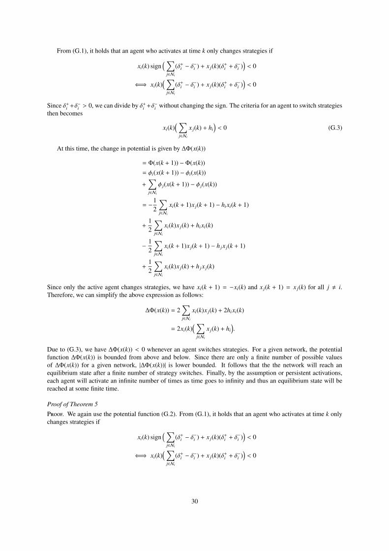
From (G.1), it holds that an agent who activates at time k only changes strategies if

xi(k) sign( ∑

j∈Ni

(δ+i − δ

−i ) + x j(k)(δ+

i + δ−i ))< 0

⇐⇒ xi(k)( ∑

j∈Ni

(δ+i − δ

−i ) + x j(k)(δ+

i + δ−i ))< 0

Since δ+i +δ−i > 0, we can divide by δ+

i +δ−i without changing the sign. The criteria for an agent to switch strategiesthen becomes

xi(k)( ∑

j∈Ni

x j(k) + hi

)< 0 (G.3)

At this time, the change in potential is given by ∆Φ(x(k))

= Φ(x(k + 1)) − Φ(x(k))= φi(x(k + 1)) − φi(x(k))

+∑j∈Ni

φ j(x(k + 1)) − φ j(x(k))

= −12

∑j∈Ni

xi(k + 1)x j(k + 1) − hixi(k + 1)

+12

∑j∈Ni

xi(k)x j(k) + hixi(k)

−12

∑j∈Ni

xi(k + 1)x j(k + 1) − h jx j(k + 1)

+12

∑j∈Ni

xi(k)x j(k) + h jx j(k)

Since only the active agent changes strategies, we have xi(k + 1) = −xi(k) and x j(k + 1) = x j(k) for all j , i.Therefore, we can simplify the above expression as follows:

∆Φ(x(k)) = 2∑j∈Ni

xi(k)x j(k) + 2hixi(k)

= 2xi(k)( ∑

j∈Ni

x j(k) + hi

).

Due to (G.3), we have ∆Φ(x(k)) < 0 whenever an agent switches strategies. For a given network, the potentialfunction ∆Φ(x(k)) is bounded from above and below. Since there are only a finite number of possible valuesof ∆Φ(x(k)) for a given network, |∆Φ(x(k))| is lower bounded. It follows that the the network will reach anequilibrium state after a finite number of strategy switches. Finally, by the assumption or persistent activations,each agent will activate an infinite number of times as time goes to infinity and thus an equilibrium state will bereached at some finite time.

Proof of Theorem 5

Proof. We again use the potential function (G.2). From (G.1), it holds that an agent who activates at time k onlychanges strategies if

xi(k) sign( ∑

j∈Ni

(δ+i − δ

−i ) + x j(k)(δ+

i + δ−i ))< 0

⇐⇒ xi(k)( ∑

j∈Ni

(δ+i − δ

−i ) + x j(k)(δ+

i + δ−i ))< 0

30

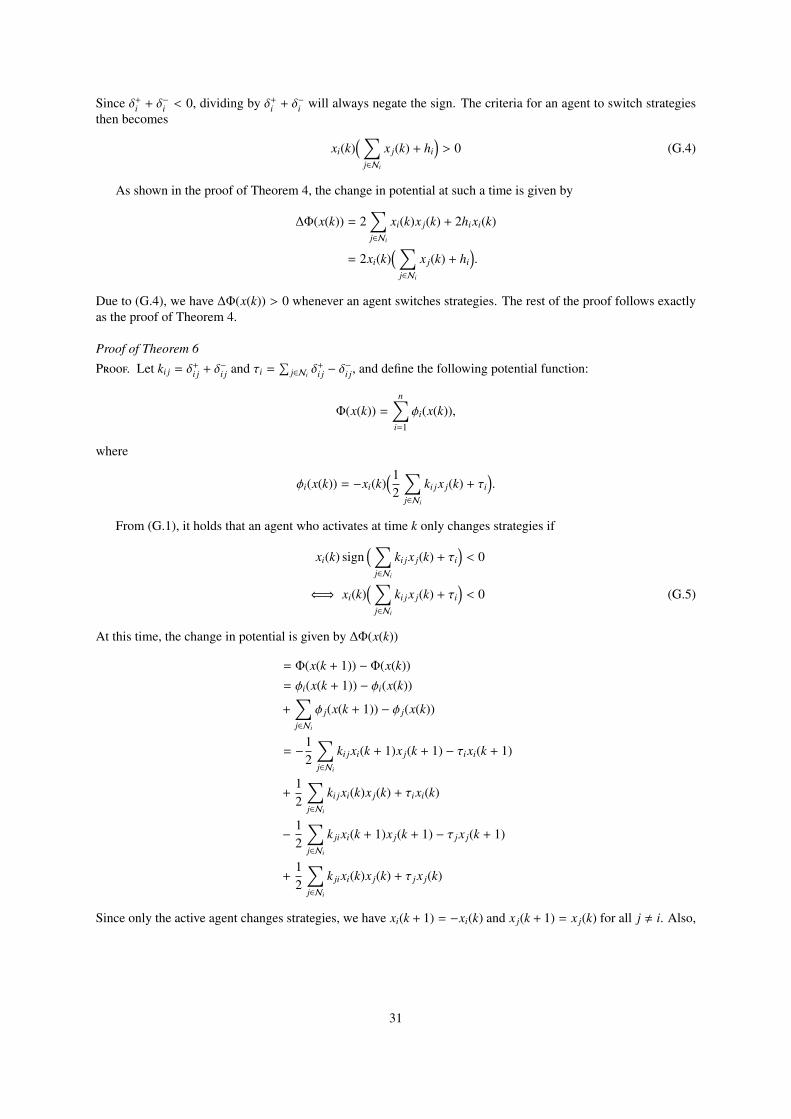
Since δ+i + δ−i < 0, dividing by δ+

i + δ−i will always negate the sign. The criteria for an agent to switch strategiesthen becomes

xi(k)( ∑

j∈Ni

x j(k) + hi

)> 0 (G.4)

As shown in the proof of Theorem 4, the change in potential at such a time is given by

∆Φ(x(k)) = 2∑j∈Ni

xi(k)x j(k) + 2hixi(k)

= 2xi(k)( ∑

j∈Ni

x j(k) + hi

).

Due to (G.4), we have ∆Φ(x(k)) > 0 whenever an agent switches strategies. The rest of the proof follows exactlyas the proof of Theorem 4.

Proof of Theorem 6

Proof. Let ki j = δ+i j + δ−i j and τi =

∑j∈Ni

δ+i j − δ

−i j, and define the following potential function:

Φ(x(k)) =

n∑i=1

φi(x(k)),

where

φi(x(k)) = −xi(k)(12

∑j∈Ni

ki jx j(k) + τi

).

From (G.1), it holds that an agent who activates at time k only changes strategies if

xi(k) sign( ∑

j∈Ni

ki jx j(k) + τi

)< 0

⇐⇒ xi(k)( ∑

j∈Ni

ki jx j(k) + τi

)< 0 (G.5)

At this time, the change in potential is given by ∆Φ(x(k))

= Φ(x(k + 1)) − Φ(x(k))= φi(x(k + 1)) − φi(x(k))

+∑j∈Ni

φ j(x(k + 1)) − φ j(x(k))

= −12

∑j∈Ni

ki jxi(k + 1)x j(k + 1) − τixi(k + 1)

+12

∑j∈Ni

ki jxi(k)x j(k) + τixi(k)

−12

∑j∈Ni

k jixi(k + 1)x j(k + 1) − τ jx j(k + 1)

+12

∑j∈Ni

k jixi(k)x j(k) + τ jx j(k)

Since only the active agent changes strategies, we have xi(k + 1) = −xi(k) and x j(k + 1) = x j(k) for all j , i. Also,

31

since all games are symmetric, ki j = k ji. Therefore, we can simplify the above expression as follows:

∆Φ(x(k)) = 2∑j∈Ni

ki jxi(k)x j(k) + 2τixi(k)

= 2xi(k)( ∑

j∈Ni

ki jx j(k) + τi

).

Due to (G.5), we have ∆Φ(x(k)) < 0 whenever an agent switches strategies. For a given network, the potentialfunction ∆Φ(x(k)) is bounded from above and below. Since there are only a finite number of possible valuesof ∆Φ(x(k)) for a given network, |∆Φ(x(k))| is lower bounded. It follows that the the network will reach anequilibrium state after a finite number of strategy switches. Finally, since the activation sequence is persistent,each agent will activate an infinite number of times as time goes to infinity and thus the equilibrium state will bereached at some finite time.

32