analysis of evolutionary algorithms in the control of path
TRANSCRIPT

Wright State University Wright State University
CORE Scholar CORE Scholar
Browse all Theses and Dissertations Theses and Dissertations
2018
Analysis of Evolutionary Algorithms in the Control of Path Analysis of Evolutionary Algorithms in the Control of Path
Planning Problems Planning Problems
Pavlos Androulakakis Wright State University
Follow this and additional works at: https://corescholar.libraries.wright.edu/etd_all
Part of the Electrical and Computer Engineering Commons
Repository Citation Repository Citation Androulakakis, Pavlos, "Analysis of Evolutionary Algorithms in the Control of Path Planning Problems" (2018). Browse all Theses and Dissertations. 2026. https://corescholar.libraries.wright.edu/etd_all/2026
This Thesis is brought to you for free and open access by the Theses and Dissertations at CORE Scholar. It has been accepted for inclusion in Browse all Theses and Dissertations by an authorized administrator of CORE Scholar. For more information, please contact [email protected].
Analysis of Evolutionary Algorithms in the Controlof Path Planning Problems
A Thesis submitted in partial fulfillmentof the requirements for the degree of
Master of Science in Electrical Engineering
by
Pavlos AndroulakakisB.S.E.E., Ohio State University, 2014
2018Wright State University

Wright State UniversityGRADUATE SCHOOL
August 31, 2018
I HEREBY RECOMMEND THAT THE THESIS PREPARED UNDER MY SUPER-VISION BY Pavlos Androulakakis ENTITLED Analysis of Evolutionary Algorithms inthe Control of Path Planning Problems BE ACCEPTED IN PARTIAL FULFILLMENTOF THE REQUIREMENTS FOR THE DEGREE OF Master of Science in Electrical En-gineering.
Zachariah Fuchs, Ph.D.Thesis Director
Brian Rigling, Ph.D.Chair, Department of Electrical Engineering
Committee onFinal Examination
John C. Gallagher, Ph.D.
Luther Palmer, Ph.D.
Zachariah Fuchs, Ph.D.
Barry Milligan, Ph.D.Interim Dean of the Graduate School

ABSTRACT
Androulakakis, Pavlos. M.S.E.E., Department of Electrical Engineering, Wright State University,2018. Analysis of Evolutionary Algorithms in the Control of Path Planning Problems.
The purpose of this thesis is to examine the ability of evolutionary algorithms (EAs)
to develop near optimal solutions to three different path planning control problems. First,
we begin by examining the evolution of an open-loop controller for the turn-circle intercept
problem. We then extend the evolutionary methodology to develop a solution to the closed-
loop Dubins Vehicle problem. Finally, we attempt to evolve a closed-loop solution to the
turn constrained pursuit evasion problem.
For each of the presented problems, a custom controller representation is used. The
goal of using custom controller representations (as opposed to more standard techniques
such as neural networks) is to show that simple representations can be very effective if
problem specific knowledge is used. All of the custom controller representations described
in this thesis can be easily implemented in any modern programming language without any
extra toolboxes or libraries.
A standard EA is used to evolve populations of these custom controllers in an attempt
to generate near optimal solutions. The evolutionary framework as well as the process of
mixing and mutation is described in detail for each of the custom controller representa-
tions. In the problems where an analytically optimal solution exists, the resulting evolved
controllers are compared to the known optimal solutions so that we can quantify the EA’s
performance. A breakdown of the evolution as well as plots of the resulting evolved trajec-
tories are shown for each of the analyzed problems.
iii

Contents
1 Introduction 11.1 Traditional Solutions . . . . . . . . . . . . . . . . . . . . . . . . . . . . . 11.2 Evolutionary Algorithms . . . . . . . . . . . . . . . . . . . . . . . . . . . 21.3 Thesis Overview . . . . . . . . . . . . . . . . . . . . . . . . . . . . . . . 4
2 Open-loop evolution 52.1 Turn-Circle Intercept Control . . . . . . . . . . . . . . . . . . . . . . . . . 5
2.1.1 Problem Description . . . . . . . . . . . . . . . . . . . . . . . . . 6System Model . . . . . . . . . . . . . . . . . . . . . . . . . . . . 6Controller Design . . . . . . . . . . . . . . . . . . . . . . . . . . . 7Utility . . . . . . . . . . . . . . . . . . . . . . . . . . . . . . . . . 10Problem Definition . . . . . . . . . . . . . . . . . . . . . . . . . . 12
2.1.2 Evolutionary Architecture . . . . . . . . . . . . . . . . . . . . . . 12Controller Encoding . . . . . . . . . . . . . . . . . . . . . . . . . 12Initial Population . . . . . . . . . . . . . . . . . . . . . . . . . . . 13Crossing . . . . . . . . . . . . . . . . . . . . . . . . . . . . . . . 14Mutation . . . . . . . . . . . . . . . . . . . . . . . . . . . . . . . 15
2.1.3 Results and Analysis . . . . . . . . . . . . . . . . . . . . . . . . . 17Basic Air Combat Tactics . . . . . . . . . . . . . . . . . . . . . . 17Evolved Lag Pursuit . . . . . . . . . . . . . . . . . . . . . . . . . 19Evolved Lead Pursuit . . . . . . . . . . . . . . . . . . . . . . . . . 23Intercept Trajectory . . . . . . . . . . . . . . . . . . . . . . . . . . 25Impact of Results . . . . . . . . . . . . . . . . . . . . . . . . . . . 27
3 Closed-loop evolution 283.1 Dubins Vehicle . . . . . . . . . . . . . . . . . . . . . . . . . . . . . . . . 28
3.1.1 Problem Description . . . . . . . . . . . . . . . . . . . . . . . . . 29System Model . . . . . . . . . . . . . . . . . . . . . . . . . . . . 29Terminal Conditions . . . . . . . . . . . . . . . . . . . . . . . . . 31Game Utility . . . . . . . . . . . . . . . . . . . . . . . . . . . . . 33
3.1.2 Controller Design . . . . . . . . . . . . . . . . . . . . . . . . . . . 343.1.3 Evolutionary Architecture . . . . . . . . . . . . . . . . . . . . . . 38
iv

Evaluation . . . . . . . . . . . . . . . . . . . . . . . . . . . . . . 38Fitness . . . . . . . . . . . . . . . . . . . . . . . . . . . . . . . . 40Creating Next Generation . . . . . . . . . . . . . . . . . . . . . . 40Copies of Elite Controllers . . . . . . . . . . . . . . . . . . . . . . 41Fitness-Based Crossing of Two Controllers . . . . . . . . . . . . . 41
3.1.4 Results and Analysis . . . . . . . . . . . . . . . . . . . . . . . . . 433.1.5 Dubins Vehicle Optimal Solution . . . . . . . . . . . . . . . . . . 43
Analysis of Evolution . . . . . . . . . . . . . . . . . . . . . . . . 45Results of Evolutionary Algorithm . . . . . . . . . . . . . . . . . . 52Further Analysis . . . . . . . . . . . . . . . . . . . . . . . . . . . 54
3.1.6 Impact of Results . . . . . . . . . . . . . . . . . . . . . . . . . . . 583.2 Pursuit Evasion . . . . . . . . . . . . . . . . . . . . . . . . . . . . . . . . 58
3.2.1 Problem Description . . . . . . . . . . . . . . . . . . . . . . . . . 59System Model . . . . . . . . . . . . . . . . . . . . . . . . . . . . 59Relative Coordinates . . . . . . . . . . . . . . . . . . . . . . . . . 61Terminal Conditions . . . . . . . . . . . . . . . . . . . . . . . . . 62Game Utility . . . . . . . . . . . . . . . . . . . . . . . . . . . . . 63
3.2.2 Controller Design . . . . . . . . . . . . . . . . . . . . . . . . . . . 653.2.3 Evolutionary Architecture . . . . . . . . . . . . . . . . . . . . . . 67
Competition . . . . . . . . . . . . . . . . . . . . . . . . . . . . . 68Fitness . . . . . . . . . . . . . . . . . . . . . . . . . . . . . . . . 69Creating Next Generation . . . . . . . . . . . . . . . . . . . . . . 71Copies of Elite Controllers . . . . . . . . . . . . . . . . . . . . . . 72Mutations of Elite Controllers . . . . . . . . . . . . . . . . . . . . 72Crossing of Two Random Controllers . . . . . . . . . . . . . . . . 73Random New Controllers . . . . . . . . . . . . . . . . . . . . . . 75
3.2.4 Numerical Results and Analysis . . . . . . . . . . . . . . . . . . . 75Untrained Starting Positions . . . . . . . . . . . . . . . . . . . . . 82
3.2.5 Impact of Results . . . . . . . . . . . . . . . . . . . . . . . . . . . 83
4 Conclusion and Future Work 854.1 Conclusion . . . . . . . . . . . . . . . . . . . . . . . . . . . . . . . . . . 854.2 Future Work . . . . . . . . . . . . . . . . . . . . . . . . . . . . . . . . . . 85
Bibliography 86
v

List of Figures
2.1 Global Coordinates . . . . . . . . . . . . . . . . . . . . . . . . . . . . . . 62.2 Desired Separation . . . . . . . . . . . . . . . . . . . . . . . . . . . . . . 102.3 Creating Next Generation . . . . . . . . . . . . . . . . . . . . . . . . . . . 132.4 Crossing Examples . . . . . . . . . . . . . . . . . . . . . . . . . . . . . . 152.5 Lead Pursuit . . . . . . . . . . . . . . . . . . . . . . . . . . . . . . . . . . 182.6 Lag Pursuit . . . . . . . . . . . . . . . . . . . . . . . . . . . . . . . . . . 192.7 Utility Summary . . . . . . . . . . . . . . . . . . . . . . . . . . . . . . . 202.8 Evaluation of Evolution . . . . . . . . . . . . . . . . . . . . . . . . . . . . 212.9 Evolved 3 Segment Lag Pursuit . . . . . . . . . . . . . . . . . . . . . . . . 232.10 Evolved Lead Pursuit (7 Seg) . . . . . . . . . . . . . . . . . . . . . . . . . 242.11 Evolved Lead Pursuit (3 Seg) . . . . . . . . . . . . . . . . . . . . . . . . . 242.12 Evolved 3 Segment Lead Pursuit
(ρA = π
6
). . . . . . . . . . . . . . . . . . 25
2.13 Evolved Intercept Trajectory (7 Segments) . . . . . . . . . . . . . . . . . . 262.14 Evolved Intercept Trajectory (3 Segments) . . . . . . . . . . . . . . . . . . 26
3.1 Global Coordinates . . . . . . . . . . . . . . . . . . . . . . . . . . . . . . 293.2 Relative Coordinates . . . . . . . . . . . . . . . . . . . . . . . . . . . . . 303.3 Buffer Zones . . . . . . . . . . . . . . . . . . . . . . . . . . . . . . . . . 313.4 Terminal Condition X1 Example . . . . . . . . . . . . . . . . . . . . . . . 323.5 Example of a 4x4x4 Grid Controller . . . . . . . . . . . . . . . . . . . . . 363.6 Matrix form of the 4x4x4 Grid Controller in Figure 3.5 . . . . . . . . . . . 373.7 Initial Conditions . . . . . . . . . . . . . . . . . . . . . . . . . . . . . . . 393.8 Population Generation Method . . . . . . . . . . . . . . . . . . . . . . . . 413.9 Turn-Straight-Turn (TST) Solution . . . . . . . . . . . . . . . . . . . . . . 443.10 Turn-Turn-Turn (TTT) Solution . . . . . . . . . . . . . . . . . . . . . . . 443.11 Fitness Throughout the Evolution . . . . . . . . . . . . . . . . . . . . . . 453.12 Fitness and Success from Gen 1 to 500 . . . . . . . . . . . . . . . . . . . . 463.13 Fitness and Success Gen 500 to 5000 . . . . . . . . . . . . . . . . . . . . . 473.14 Summary of Successful Captures . . . . . . . . . . . . . . . . . . . . . . . 483.15 Generation 1 . . . . . . . . . . . . . . . . . . . . . . . . . . . . . . . . . . 493.16 Generation 25 . . . . . . . . . . . . . . . . . . . . . . . . . . . . . . . . . 493.17 Generation 145 . . . . . . . . . . . . . . . . . . . . . . . . . . . . . . . . 493.18 Generation 481 . . . . . . . . . . . . . . . . . . . . . . . . . . . . . . . . 50
vi

3.19 Generation 1698 . . . . . . . . . . . . . . . . . . . . . . . . . . . . . . . . 503.20 Generation 5000 . . . . . . . . . . . . . . . . . . . . . . . . . . . . . . . . 503.21 Performance of Best Controller from Trained IC . . . . . . . . . . . . . . . 533.22 Evolved TTT Solution vs Optimal TTT Solution . . . . . . . . . . . . . . . 543.23 Evolved TST Solution vs Optimal TST Solution . . . . . . . . . . . . . . . 543.24 Performance from Untrained IC . . . . . . . . . . . . . . . . . . . . . . . 553.25 Example of Grid Parameterization Error . . . . . . . . . . . . . . . . . . . 563.26 Evolved vs Discretized Dubins . . . . . . . . . . . . . . . . . . . . . . . . 573.27 Global Coordinates . . . . . . . . . . . . . . . . . . . . . . . . . . . . . . 603.28 Example player . . . . . . . . . . . . . . . . . . . . . . . . . . . . . . . . 613.29 Relative Coordinates . . . . . . . . . . . . . . . . . . . . . . . . . . . . . 623.30 Example of capture conditions . . . . . . . . . . . . . . . . . . . . . . . . 643.31 Three Anchor Points Subdividing a 2D Space . . . . . . . . . . . . . . . . 663.32 Initial Conditions (not to scale) . . . . . . . . . . . . . . . . . . . . . . . . 703.33 Averaging of sub-fitnesses into category fitnesses and cumulative fitness . . 713.34 Population Generation Method . . . . . . . . . . . . . . . . . . . . . . . . 723.35 Fitness over 50 generations . . . . . . . . . . . . . . . . . . . . . . . . . . 763.36 Performance of Best Controller in Generation 3 . . . . . . . . . . . . . . . 773.37 Performance of Best Controller in Generation 5 . . . . . . . . . . . . . . . 773.38 Performance of Best Controller in Generation 7 . . . . . . . . . . . . . . . 783.39 Performance of Best Controller in Generation 12 . . . . . . . . . . . . . . 783.40 Performance of Best Controller in Generation 50 . . . . . . . . . . . . . . 803.41 Anchor Points of Best Controller in Generation 50 . . . . . . . . . . . . . . 813.42 Best Controller Against Aggressive Opponent in Untrained Initial Conditions 823.43 Best Controller Against Always Straight Opponent in Untrained Initial
Conditions . . . . . . . . . . . . . . . . . . . . . . . . . . . . . . . . . . . 833.44 Player A Gets Captured by Player B from Untrained Initial Conditions . . . 84
vii

AcknowledgmentsI would like to take this opportunity to extend my thanks to Dr. Fuchs. His support and
guidance were integral parts of making this thesis possible.
I would also like to thank Dr. Gallagher and Dr. Palmer for taking the time to be part
of my committee.
viii

Dedicated to
Stavros and Voula Androulakakis
ix
Introduction
Autonomous systems are becoming increasingly prevalent in many aspects of modern life.
From military applications and space exploration, to self driving cars and logistics plan-
ning, these systems are an integral part of our advanced technologies. Path planning in
particular is a challenging task faced by most autonomous systems. Driverless cars and
UAVs must maneuver through their environments in a timely manner while satisfying dy-
namic and energy constraints. In cases where multiple agents are involved, teamwork and
adversarial tactics come into play. Often times these types of problems can be solved us-
ing analytical methods. However as the problems become more complex, this becomes
difficult. Developing a numeric methodology that is able to generate effective controllers
for these types of problems would be very useful to future control research. This thesis
examines the ability of one such numeric method, evolutionary algorithms, to develop near
optimal solutions to an array of control problems.
1.1 Traditional Solutions
There is a long history of using analytic optimal control methods for analyzing path plan-
ning problems. For example, the case in which a single turn constrained attacker is pursuing
a stationary target is referred to as the Dubins Vehicle problem and has been analytically
solved by Lester E. Dubins [1]. More complex scenarios in which a mobile target is able to
move around and act in direct opposition to the attacker have been examined from a game
1

theoretic perspective and solved as shown in [2], [3], [4].
Although analytic methods provide the true equilibrium solution, it may not always be
possible to analytically derive optimal solutions for realistic problems with highly nonlin-
ear dynamics. Additionally, classical optimization techniques may not scale well for high
dimensional systems. In these situations, numerical optimizations techniques provide an
effective method of getting near optimal solutions. Evolutionary algorithms are particularly
useful for searching these large and often complex solution spaces.
1.2 Evolutionary Algorithms
Evolutionary algorithms (EAs) use the principles of natural selection and fitness to evolve a
population of candidate solutions over a series of generations. These algorithms have been
successfully implemented in a wide range of optimization problems. For example, in [5]
the authors used an evolutionary algorithm to optimize air traffic control patterns. In [6],
the authors used a combination of two evolutionary algorithms to develop control schemes
for robots with complex locomotor systems.
The focus of this thesis is on the application of evolutionary algorithms to path plan-
ning problems. In general, there are two types of solutions that can be developed; open-loop
solutions and closed-loop solutions.
Open-loop solutions take in an initial state and will return a control for any requested
time u = f(x0, t). For example, [7] uses an advanced evolutionary algorithm to evolve
a sequence of waypoints that an agent follows to help navigate an obstacle rich environ-
ment. The process of evolving open-loop solutions is extremely effective at solving for a
near optimal solution from any given initial condition, however the resulting evolved con-
troller is only valid for that specific initial condition. If the solution from a different initial
condition is desired, then the evolutionary algorithm would need to be rerun from the new
location. This can be a problem for fast moving real world systems. The authors of [8]
2

address this problem by implementing a fast evolutionary algorithm on an FPGA that is
able to develop new open-loop solutions for a UAV in under 100ms. This allows them to
constantly update their trajectory by using their current state as a new initial condition. As
shown in their paper, this method allows them to effectively control the UAV. While these
types of online open-loop solutions can be very effective, they are limited by on-board
computational power and algorithm complexity. Closed loop solutions are able to address
this shortcoming at the cost of added complexity in controller representation.
Unlike open-loop solutions, closed-loop solutions are a function of our current state
u = f(x(t)) rather than our initial state u = f(x0, t). Instead of developing a solution from
one initial condition, a closed-loop solution is able to provide a solution for all admissible
states. Theoretically this allows us to evolve a feedback controller once and have a solution
for all admissible states. The system implementing the feedback controller would then have
the flexibility to update its control as fast as it can evaluate u = f(x(t)).
In order to evolve a feedback controller, we will need to be able to parameterize it. One
way to do this is to directly evolve the parameters of existing feedback control methods.
The authors of [9] use this method to evolve the coefficients of a PID controller. Another
method of parameterization that has drawn the focus of many researchers is the neural
network [10], [11], [12], [13], [14]. Due to their universal approximation property, neural
networks are theoretically able to represent any possible controller. Since evolutionary
algorithms are exploring large spaces for an unknown solution, being able to guarantee
that no solution is unrepresentable by the controller representation (in this case a neural
network) is very important. The drawback with neural networks is the relative complexity
of their implementation and evolution. Many toolboxes and software libraries have been
developed that make this process easier, but the complexity of the fundamental design
choices are still present. With enough experience and knowledge neural networks are a
very powerful tool, but in some problems they may be more than is necessary.
This thesis explores alternative controller representations that are custom built for the
3

problem at hand. These representations range from something as simple as a look up table
to slightly more sophisticated methods such as a nearest neighbor kd search tree. The goal
of using these non-standard representations is to show that even though these new represen-
tations are simple, they are still able to develop near optimal solutions. Additionally, these
controllers can be implemented in most modern programming languages with no additional
libraries or toolboxes.
1.3 Thesis Overview
This thesis is broken up into four chapters. Chapter 1 contains the introduction and a
brief overview of current research in this area. Chapter 2 focuses on a standard open-
loop path planning control problem that will allow us to validate the EA methodology. The
research shown in Chapter 2 focuses on the turn circle intercept problem and was presented
at the 2018 IEEE World Congress on Evolutionary Computation. Chapter 3 focuses on two
closed-loop path planning control problems. The first of these problems is the closed-
loop Dubins Vehicle problem. The Dubins Vehicle problem has a well defined empirical
solution that is used to validate our closed-loop evolutionary algorithm. The second of the
two problems is the more complex Pursuit Evasion problem. This problem is the most
challenging test of our methodology and serves as an example of how an EA can be used
to generate solutions to problems in which the target is moving with unknown behavior.
The research for this problem was presented at the 2017 IEEE Congress on Evolutionary
Computation. Chapter 4 contains the conclusion and ideas for future work.
4

Open-loop evolution
In this section we attempt to evolve an open-loop controller. Open loop controllers are
defined as controllers that do not have any state feedback. In other words, open-loop con-
trollers do not use the state of the system in the computation of the control. This makes
the encoding of the controller for the purposes of crossing and mutation in an evolutionary
algorithm relatively easy. The goal of this chapter is to validate the evolutionary framework
by testing it on a relatively basic control problem in which the optimal solution is know.
2.1 Turn-Circle Intercept Control
This section focuses on the turn-circle intercept problem. This problem is a fundamental
part of air-to-air combat and formation maintenance problems. Due to its relative simplicity
and wide set of applications, this problem has been heavily researched and many strategies
and tactics for how pilots should respond based on the relative configuration of the Attacker
and Target have been empirically developed [15]. Lead and Lag pursuit represent two of
the most fundamental techniques and can be used to maneuver an attacker into a desired
position in minimum time. The goal of this section is to use an evolutionary algorithm to
create an open-loop controller that is able to reproduce these empirically optimal solutions.
5

θ
θ
Figure 2.1: Global Coordinates
2.1.1 Problem Description
The problem considers two agents, the Attacker and Target, moving about an obstacle-
free, two-dimensional plane. The Target moves with constant speed and turn-rate, which
results in a circular trajectory with fixed turn-radius and center. The Attacker also moves
with constant speed, but is free to choose its turn-rate in an effort to capture the Target in
minimum time. Successful capture occurs when the Attacker maneuvers into a position
behind the Target on the same turn circle. The objective of the problem is to identify a
control strategy for the Attacker that achieves capture in minimum time.
System Model
The Attacker’s state is defined by its position, (xA, yA), and heading angle, θA. Similarly,
the Target’s state is defined by its position, (xT, yT), and heading angle, θT . A summary of
this two agent system is shown in Figure 2.1. The complete state of the system, x, will be
referred to as the global state and is defined as the collection of the individual agent states
6
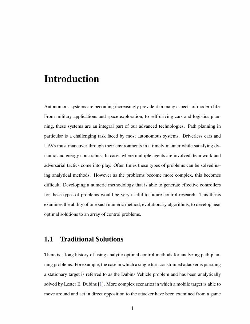
as well as a time state τ :
x := (xA, yA, θA, xT, yT, θT, τ). (2.1)
The system dynamics x := f(x, uA, uT) are defined by a system of seven ordinary
differential equations:
xA := vA cos(θA) (2.2)
yA := vA sin(θA) (2.3)
θA := vAρAuA (2.4)
xT := vT cos(θT) (2.5)
yT := vT sin(θT) (2.6)
θT := vTρTuT (2.7)
τ := 1, (2.8)
where the constants vA > 0 and vT > 0 are the Attacker and Target’s respective speeds. The
constants ρA > 0 and ρT > 0 are the Attacker and Target’s turn radii. The Attacker controls
its heading through uA ∈ [−1, 1], and the Target controls its heading through uT ∈ [−1, 1].
We define the state at initial time t0 as x(t0) = x0 := (xA0, yA0, θA0, xT0, yT0, θT0, τ0).
Controller Design
In the turn circle intercept problem, the target is assumed to be constantly turning in a
circle. To accomplish this, we arbitrarily assign the Target a constant turn rate of uT(t) = 1
(turn right). Using the assumed control strategy and initial condition, the Target’s trajectory
7

can be calculated by integrating the dynamics (2.5)-(2.7) with respect to time:
xT(t;x0) = xT0 − ρT sin θT0 + ρT sin(θT0 + vTρTt) (2.9)
yT(t;x0) = yT0 + ρT cos θT0 − ρT cos(θT0 + vTρTt) (2.10)
θT(t;x0) = θT0 + vTρTt. (2.11)
This results in a circular trajectory with a center located at
(xc, yc) := (xT0 − ρT sin θT0, yT0 + ρT cos θT0) (2.12)
and a radius of ρT .
Previous analysis of problems with similar dynamics [16, 17, 18] has shown that the
optimal control strategies typically possess a bang-zero-bang structure, in which the agent
implements either a hard left-turn uA = 1, no turn uA = 0, or a hard right-turn uA = −1.
Therefore, we represent the Attacker’s control strategy as a piecewise constant function of
time consisting of N segments:
uA(t;CA) =
u1 0 ≤ t < t1
u2 t1 ≤ t < t2
u3 t2 ≤ t < t3...
...
uN tN−1 ≤ t < tN
0 tN ≤ t,
(2.13)
where the parameter set CA := {{u1, u2, . . . , uN}, {t1, t2, . . . , tN}} contains the control,
8

ui ∈ {−1, 0, 1}, and segment times, ti ≥ 0. The control structure assumes that
0 ≤ t1 ≤ t2 ≤ · · · ≤ tN . (2.14)
Substituting the Attacker’s control into the Attacker dynamics (2.2)-(2.4) and integrat-
ing provides the Attacker’s trajectory as a function of time:
xA(t;x0,CA) =
xAi − ρA sin θAi + ρA sin(θAi + vA
ρA(t− ti)) ui+1 = 1
xAi + vA cos(θAi)(t− ti) ui+1 = 0
xAi + ρA sin θAi − ρA sin(θAi − vAρA
(t− ti)) ui+1 = −1
(2.15)
yA(t;x0,CA) =
yAi + ρA cos θAi − ρA cos(θAi + vA
ρA(t− ti)) ui+1 = 1
yAi + vA sin(θAi)(t− ti) ui+1 = 0
yAi − ρA cos θAi + ρA cos(θAi − vAρA
(t− ti)) ui+1 = −1
(2.16)
θA(t;x0,CA) =
θAi + vA
ρA(t− ti) ui+1 = 1
θAi ui+1 = 0
θAi − vAρA
(t− ti) ui+1 = −1
(2.17)
where the index i satisfies i = arg maxi ti < t and the intermediate state components are
computed recursively as xAi = xA(ti;x0,CA), yAi = yA(ti;x0,CA), and θAi = θA(t0;x0,CA).
The initial conditions are defined as xA(t0;x0,CA) = xA0, yA(t0;x0,CA) = yA0, and θA(t0;x0,CA) =
θA0.
9

Target
)
Figure 2.2: Desired Separation
Utility
Given an initial condition x0, control parameter set CA, and terminal time tf , the final sys-
tem state, xf , is computed using the trajectories defined in (2.9)-(2.11) and (2.15)-(2.17):
xf (CA, tf ) := (xTf , yTf , θTf , xAf , yAf , θAf , tf ) (2.18)
= (xT(tf ;x0), yT(tf ;x0), θT(tf ;x0), xA(tf ;x0,CA), yA(tf ;x0,CA), θA(tf ;x0,CA), tf ) .
(2.19)
For this problem, the terminal time is assumed to be the maximum time of the final control
segment: tf = tN .
The Attacker strives to maneuver into a position behind the Target, which is both on
the Target’s turn circle and at a desired separation distance as shown in Figure 2.2. The
desired separation between the Target and Attacker is defined in terms of angle α. Using
10

these conditions, the desired (x,y) coordinates of the Attacker can be expressed as
x = (xTf − xc) cos(α)− (yTf − yc) sin(α) + xc (2.20)
y = (yTf − yc) cos(α) + (xTf − xc) sin(α) + yc, (2.21)
where xc and yc are the coordinates of the center of the Target’s turn circle as defined in
(2.12). We define an error function in terms of the Attacker’s terminal distance from the
desired position:
h1(xf ; α) :=√
(x− xAf )2 + (y − yAf )2. (2.22)
An additional constraint on the Attacker’s terminal heading is imposed to require tangential
motion to the Target’s turn circle:
h2(xf ) := (2.23)√(cos(θAf )− cos(θTf + α))2 + (sin(θAf )− sin(θTf + α))2.
Since the Attacker strives to minimize the total elapsed time to capture, we define a time
based utility function that consists of the total elapsed time of all control segments:
h3(xf ;CA) = tN (2.24)
The overall utility function is a weighted sum of all three utilities:
U(CA) = w1h1 + w2h2 + w3h3, (2.25)
where w1, w2, and w3 are positive weight coefficients. Adjusting the relative magnitudes
of the weights prioritizes satisfying the terminal constraints or minimizing total time
11
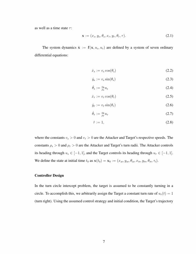
Problem Definition
Using the overall utility function (2.25), we can state the trajectory optimization problem
in terms of a minimization over the Attacker’s parameter set:
minCA
U(CA). (2.26)
The resulting optimal parameter set C∗A is used to define the optimal Attacker control strat-
egy u∗A(t) = uA(t;C∗A). The optimization problem defined in (2.26) contains both integer,
{u1, u2, . . . , uN}, and continuous variables, {t1, t2, . . . , tN}, which can be very challeng-
ing to solve using traditional optimization techniques. In Section 2.1.2, we present an
evolutionary algorithm method for solving this optimization problem that simultaneously
explores the integer and continuous parameter domains.
2.1.2 Evolutionary Architecture
The Attacker control parameter set, C, contains both integer and continuous values. Addi-
tionally, these parameters are closely coupled in how they influence the overall trajectory
of the Attacker and resulting utility. In order to simultaneously explore both the discrete
and continuous parameter space, we employ an evolutionary algorithm.
Controller Encoding
In order to satisfy the ordering constraint (2.14), we do not directly evolve the segment
times {t1, t2, . . . , tN}. Instead, we evolve the duration of each segment through the param-
eters {∆t1,∆t2, . . . ,∆tN}, where 0 ≤ ∆ti ≤ ∆t. The maximum segment duration ∆t is
used to upper-bound the search space. When the controller is evaluated, the segment times
are computed as
ti =i∑
j=1
∆tj. (2.27)
12

Crossing
Mutation
Elite 5%
95%
Old Gen New Gen
Fitn
ess
Figure 2.3: Creating Next Generation
This implicitly ensures that ti+1 ≥ ti and thus satisfies (2.14). Therefore, a candidate
controller C = {{u1, u2, . . . , uN}, {t1, t2, . . . , tN}} is represented as
c = {{u1, u2, . . . , uN}, {∆t1,∆t2, . . . ,∆tN}} (2.28)
within the evolutionary algorithm. The task of the evolutionary algorithm is to evolve c in
order to optimize (2.26).
Initial Population
To begin, we initialize a population of M candidate controllers to serve as our first genera-
tion G0 = {c1, c2, ...cM}. These candidate controllers are initialized with random control
values uniformly drawn from the set {−1, 0, 1}, p(ui) = 1/3, and time values uniformly
selected from the range [0, tmax].
After generating the initial population, G0, the evolutionary algorithm will create gen-
eration G1 with population assigned as shown in Figure 2.3. The top 5% of the old gen-
eration are considered elite and are passed on to the next generation without any change.
This ensures that the top performing controllers persist through to the next generation and
don’t accidentally get degraded by the crossing and mutation operations. The remaining
13

95% of the next generation is filled with the results of crossing and mutation. This process
will repeat until we reach a predefined number of generations and end with generation Gf .
Crossing
Crossing begins by uniformly selecting two parent controllers, cA and cB, from the previous
generation. The child controller cC is created by crossing each segment of the parents in a
two step process. First, a segment control value is uniformly selected from the parents for
each segment:
p(uci) =
.5 uAi
.5 uBi
. (2.29)
Second, a new time is uniformly selected for each segment from a range defined by the
parent segment times:
p(∆tci) =
1
∆tmax−∆tmin∆tci ∈ [∆tmin,∆tmax]
0 otherwise, (2.30)
where
tmin = max(0, .5(∆tAi + ∆tBi)− γ1|∆tAi −∆tBi|) (2.31)
tmax = min(∆t, .5(∆tAi + ∆tBi) + γ1|∆tAi −∆tBi|). (2.32)
The lower and upper bounds defined by (2.31) and (2.32) ensure that the child times still
satisfy the parameter bounds. The growth parameter γ1 ≥ .5 introduces a mutation fac-
tor that allows the parameters to explore values beyond the bounds imposed by the parent
parameters. Figure 2.4 shows an example of distribution bounds for three different val-
ues of ∆tAi and ∆tBi. The closer ∆tAi and ∆tBi are, the smaller the range that the child’s
14

01 2 3 4 5 6 7 8
0.5 7.2
8.54
1.6 4.3
1 2 3 4
4.840.96
5.2 5.7
5.1 5.8
1
2
3
Figure 2.4: Crossing Examples
corresponding time parameter will be selected from.
Mutation
After a child parameter set is produced, random mutations are applied in order to explore
the parameter space. Each element of the control set is selected for mutation with likeli-
hood µ1. When a mutation occurs, a new control value is selected uniformly from the set
{−1, 0, 1}. The resulting distribution for control elements within the mutated control set
{um1, um2, . . . , umN} is
p(umi) =
1− µ1 umi = uci
µ13
umi ∈ {−1, 0, 1}. (2.33)
Each element of the time duration set is selected for mutation with likelihood µ2. When
a mutation occurs for a time value ∆tci, a new value is randomly selected in the range
[∆tmin,∆tmax], where ∆tmin = max(0, tci − σ) and ∆tmax = min(∆t,∆tci + σ). The
parameter σ ≥ 0 is the mutation magnitude. The resulting distribution for each duration
15

element of the mutated set {∆tm1,∆tm2, . . . ,∆tmN} is
p(∆tmi) =
1− µ2 ∆tmi = ∆tci
µ2∆tmax−∆tmin
∆tmi ∈ [∆tmin,∆tmax]. (2.34)
16

2.1.3 Results and Analysis
The results in this section are obtained by evolving a population of M = 150 candidate
controllers over 500 generations with the parameters shown below. Several parameter sets
were tested and these represent just one of the many possible parameter sets that will result
in successful evolution.
Velocity: vA = vB = 1
Maximum Turn-Rate: ρA = ρB =π
7
Desired Separation: α = −π8
Mutation Chance: µ1 = µ2 = 0.1%
Mutation Severity: σ = 0.1
Utility Weights: w1 = 10 w2 = 10 w3 = 1
In order to ensure that the resulting candidate controller is among the best solutions ob-
tainable by our algorithm, 1000 independent evolutions are performed. Since the focus of
this thesis is on the behavior of the resulting solution rather than the statistical performance
of the algorithm, only the evolution that results in the candidate controller with the lowest
overall utility is used in the analysis.
Basic Air Combat Tactics
Before examining the results of the evolutionary algorithm, we introduce three basic air
combat pursuit tactics; Lead Pursuit, Lag Pursuit, and Pure Pursuit. These general tactics
are used to adjust an agent’s position relative to a target or wingman without needing to
adjust throttle or speed [15]. In order to evaluate the performance of the evolutionary
algorithm, we evolve controllers for initial conditions that would traditionally implement
17

ଵ
ଵ
ଶ
ଶ
Figure 2.5: Lead Pursuit
one of these tactics. Although we did not explicitly impose these concepts into the structure
of the Attacker’s controller, the optimized control strategies produced by the evolutionary
algorithm exhibit qualitatively similar behaviors.
Lead pursuit allows the Attacker to close the distance between itself and the Target
by cutting inside the Target’s turn circle and traveling a shorter path. Figure 2.5 shows an
example trajectory in which lead pursuit is implemented. The markings along the trajectory
show the location of each agent at equal points in time. Lag pursuit allows the Attacker to
fall behind the Target by steering its heading outside of the Target’s turn circle. Figure 2.6a
shows an example trajectory in which lag pursuit is implemented. The Attacker increases
the distance between itself and the Target by taking a wide turn. In the case where the
Attacker starts in front of the Target, this technique can be used to reposition the Attacker
behind the target as shown in Figure 2.6b. The case in which the Attacker is exactly on
the Target’s turn circle is referred to as pure pursuit. Pure pursuit will cause the two agents
to move around in a circle together and the relative positions of the two agents to remain
18

ଵ
ଵ
ଶ
ଶ
(a) Attacker Behind
ଵଵ
ଶ ଶ
(b) Attacker In Front
Figure 2.6: Lag Pursuit
constant.
Evolved Lag Pursuit
We begin with the results of evolving a seven segment controller from initial condition
x0 = (1.575, 0.653,−π4, 0, 0, 0, 0), which represents the case were the Attacker is in front
of the Target. According to standard tactics the Attacker should implement lag pursuit in
order to fall back to the desired position.
As stated in the beginning of this section, 1000 independent evolutions were run.
These runs had an average final best evolved utility of 19.45 with a standard deviation
of 5.11. From these 1000 evolutions, the run containing the controller with the lowest
utility in generation 500 was selected for the following analysis. Figure 2.7 shows the
minimum utility achieved in each generation of the evolution. Multiple points of interest
have been marked on this plot, each of which correspond to different evolutionary leaps.
Figure 2.8 shows the trajectory, and control strategy of the best player in each of these
19

0 50 100 150 200 250 300 350 400 450 500
Generations
10
15
20
25
30
35
40
45
50
55
Util
ity
G1
G43
G136
G9
G23
G500
Figure 2.7: Utility Summary
marked generations. The trajectory plots show the Attacker’s trajectory in red and the
Target’s trajectory in blue. An x symbol indicates the initial condition. The empty circles
represent the transition time between segments of the Attacker’s controller. The larger
filled circles indicate the final positions. The thick empty black circle represents the desired
Attacker location. The control strategy (shown below each trajectory) shows how long each
control segment was implemented. A value of 1 = Left; 0 = Straight; and −1 = Right.
The ‘x’ and circle markers refer to the corresponding Attacker markers in the trajectory
plot.
In Generation 1, the Attacker randomly moves around the space. This trajectory has a
total time of 26.64 seconds and a final position and heading that are not close to the desired
state. For these reasons, the overall utility for this Attacker is very high at a value of 53.99.
We can see from the control summary, that out of the seven segments, only five control
switches were made. The last three segments were all turn left, which could also have been
accomplished by one segment with a time equal to the sum of the three segments times.
By taking advantage of this phenomenon, the EA can explore control solutions with lower
number of segments.
20

-6 -4 -2 0 2 4
x
-2
-1
0
1
2
3
4
5
6
7
y
-6 -4 -2 0 2 4
x
-2
-1
0
1
2
3
4
5
6
7
y
-6 -4 -2 0 2 4
x
-2
-1
0
1
2
3
4
5
6
7
y
0 5 10 15 20 25
Time
-1
0
1
Con
trol
(a) G1: U(c)=53.99 tf = 26.64
0 5 10 15 20 25 30
Time
-1
0
1
Con
trol
(b) G9: U(c)=39.23 tf=29.76
0 5 10 15 20
Time
-1
0
1
Con
trol
(c) G23: U(c)=29.34 tf=23.19
-6 -4 -2 0 2 4
x
-2
-1
0
1
2
3
4
5
6
7
y
-6 -4 -2 0 2 4
x
-2
-1
0
1
2
3
4
5
6
7
y
-6 -4 -2 0 2 4
x
-2
-1
0
1
2
3
4
5
6
7
y
0 2 4 6 8 10 12 14
Time
-1
0
1
Con
trol
(d) G43: U(c)=20.05 tf=13.11
0 2 4 6 8 10
Time
-1
0
1
Con
trol
(e) G136: U(c)=14.66 tf=10.9
0 2 4 6 8 10
Time
-1
0
1
Con
trol
(f) G500: U(c)=12.20 tf=10.10
Figure 2.8: Evaluation of Evolution
21
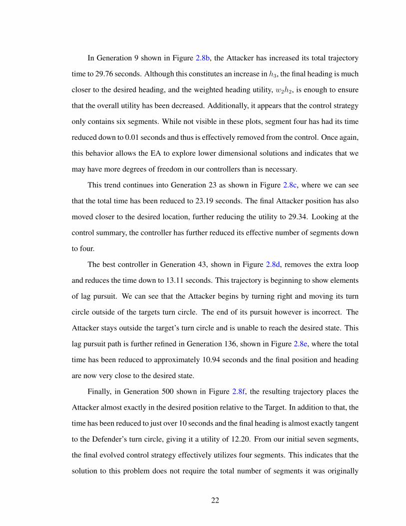
In Generation 9 shown in Figure 2.8b, the Attacker has increased its total trajectory
time to 29.76 seconds. Although this constitutes an increase in h3, the final heading is much
closer to the desired heading, and the weighted heading utility, w2h2, is enough to ensure
that the overall utility has been decreased. Additionally, it appears that the control strategy
only contains six segments. While not visible in these plots, segment four has had its time
reduced down to 0.01 seconds and thus is effectively removed from the control. Once again,
this behavior allows the EA to explore lower dimensional solutions and indicates that we
may have more degrees of freedom in our controllers than is necessary.
This trend continues into Generation 23 as shown in Figure 2.8c, where we can see
that the total time has been reduced to 23.19 seconds. The final Attacker position has also
moved closer to the desired location, further reducing the utility to 29.34. Looking at the
control summary, the controller has further reduced its effective number of segments down
to four.
The best controller in Generation 43, shown in Figure 2.8d, removes the extra loop
and reduces the time down to 13.11 seconds. This trajectory is beginning to show elements
of lag pursuit. We can see that the Attacker begins by turning right and moving its turn
circle outside of the targets turn circle. The end of its pursuit however is incorrect. The
Attacker stays outside the target’s turn circle and is unable to reach the desired state. This
lag pursuit path is further refined in Generation 136, shown in Figure 2.8e, where the total
time has been reduced to approximately 10.94 seconds and the final position and heading
are now very close to the desired state.
Finally, in Generation 500 shown in Figure 2.8f, the resulting trajectory places the
Attacker almost exactly in the desired position relative to the Target. In addition to that, the
time has been reduced to just over 10 seconds and the final heading is almost exactly tangent
to the Defender’s turn circle, giving it a utility of 12.20. From our initial seven segments,
the final evolved control strategy effectively utilizes four segments. This indicates that the
solution to this problem does not require the total number of segments it was originally
22

-3 -2 -1 0 1 2 3 4
x
-1
0
1
2
3
4
5
6
y
0 1 2 3 4 5 6 7 8 9 10
Time
-1
0
1
Con
trol
Figure 2.9: Evolved 3 Segment Lag Pursuit
given.
To test this, we reran that evolutionary algorithm with only three segments. The re-
sulting best controller’s trajectory and control summary is shown in Figure 2.9. We can see
that the this three segment solution is very similar to our seven segment solution. In fact,
the three segment solution performed slightly better by reaching the desired state with an
overall time of 9.23 seconds. This shows that the excess segments made solving the prob-
lem more complicated since the EA had to search a larger space of solutions and slowly
remove the unnecessary dimensions. Even though the evolutionary algorithm was given
more segments than necessary, it was able to remove the excess degrees of freedom and
find an efficient solution.
Evolved Lead Pursuit
Next we examine initial condition x0 := (−1.575, 0.653, π4, 0, 0, 0, 0) which places the
Attacker further behind the Target than desired. Standard doctrine states that the Attacker
23

should implement lead pursuit to catch up to the Target. The trajectory of the best evolved
Attacker using seven segments is shown in Figure 2.10. Of the seven starting segments, the
final controller only effectively utilizes two. Rerunning the evolutionary algorithm to start
with three segments, we can see that a similar solution is found as shown in Figure 2.11.
-6 -5 -4 -3 -2 -1 0 1 2 3
x
-4
-3
-2
-1
0
1
2
3
4
5
y
0 2 4 6 8 10 12 14 16 18 20
Time
-1
0
1
Con
trol
Figure 2.10: Evolved Lead Pursuit (7 Seg)
-6 -5 -4 -3 -2 -1 0 1 2 3
x
-4
-3
-2
-1
0
1
2
3
4
5
y
0 2 4 6 8 10 12 14 16 18 20
Time
-1
0
1
Con
trol
Figure 2.11: Evolved Lead Pursuit (3 Seg)
Lead pursuit is expected from this initial condition; however, the Attacker performs
what looks to be a needless loop at the beginning of its trajectory. This extra loop is
implemented because the Attacker starts on the Target’s turn circle and both Attacker and
Target have the same turn rate. Therefore, it is not possible for the Attacker to implement
lead pursuit from the start because it cannot turn sharp enough to cut into the Target’s turn
circle as shown in Figure 2.5. In our case if the Attacker started turning left in an attempt
to do this, it would simply follow the target around in pure pursuit. To solve this problem,
the evolutionary algorithm found a solution that looped the Attacker around into a position
from which it could cut into the Target’s turn circle and implement lead pursuit.
24
-6 -5 -4 -3 -2 -1 0 1 2 3
x
-4
-3
-2
-1
0
1
2
3
4
5
y
0 1 2 3 4 5 6 7 8 9
Time
-1
0
1
Con
trol
Figure 2.12: Evolved 3 Segment Lead Pursuit(ρA = π
6
)
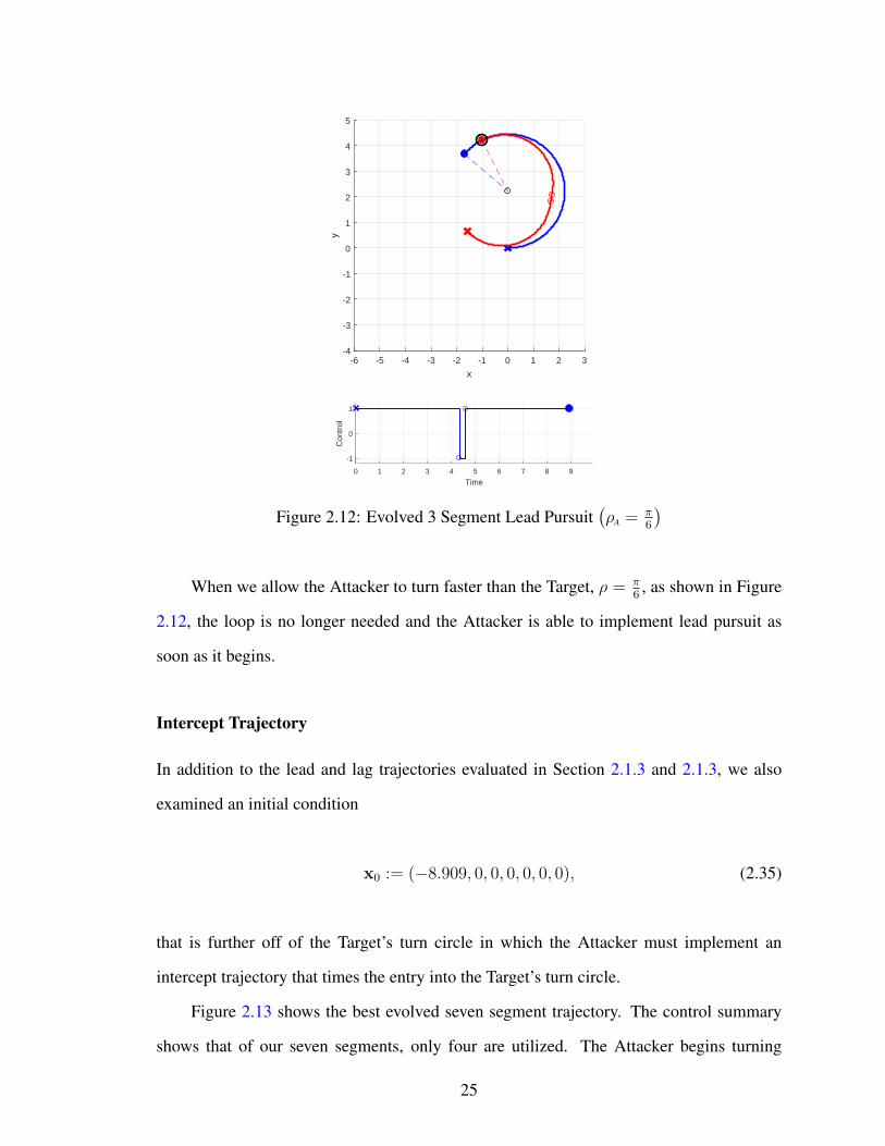
When we allow the Attacker to turn faster than the Target, ρ = π6, as shown in Figure
2.12, the loop is no longer needed and the Attacker is able to implement lead pursuit as
soon as it begins.
Intercept Trajectory
In addition to the lead and lag trajectories evaluated in Section 2.1.3 and 2.1.3, we also
examined an initial condition
x0 := (−8.909, 0, 0, 0, 0, 0, 0), (2.35)
that is further off of the Target’s turn circle in which the Attacker must implement an
intercept trajectory that times the entry into the Target’s turn circle.
Figure 2.13 shows the best evolved seven segment trajectory. The control summary
shows that of our seven segments, only four are utilized. The Attacker begins turning
25

-10 -8 -6 -4 -2 0 2
x
-1
0
1
2
3
4
5
6
y
0 2 4 6 8 10 12
Time
-1
0
1
Con
trol
Figure 2.13: Evolved Intercept Trajectory(7 Segments)
-10 -8 -6 -4 -2 0 2
x
-1
0
1
2
3
4
5
6
y
0 2 4 6 8 10 12
Time
-1
0
1
Con
trol
Figure 2.14: Evolved Intercept Trajectory(3 Segments)
the same direction as the Target until it completes about 14th of a full circle. While not
immediately evident, the attacker then begins implementing a lag pursuit strategy. In order
for the Attacker to end up behind the Target, it has to move its turn circle further out. We
can see that from t = 3.32 to t = 4.09, the Attacker moves straight. This allows the
Attacker to push its turn circle outside of the Target’s turn circle. After performing the final
turn, we can see that the Attacker is indeed behind the Target and able to reach the desired
location and heading.
Figure 2.14 shows the best evolved three segment trajectory. As with our previous
results, the three segment evolution developed a solution that is very similar to the seven
segment solution. Instead of using a straight segment to move the attackers turn circle, this
three segment solution uses a combination of turn left and turn right. Overall, this result
shows the ability of the evolutionary algorithm to utilize the underlying principles of lead
and lag pursuit to time its approach and effectively navigate to the desired state.
26

Impact of Results
Although we do not explicitly impose the concepts of lead and lag pursuit on the Attacker’s
control structure, the optimal strategies produced by our EA posses qualitatively similar be-
haviors. This result provides some validation that evolutionary algorithm is able to generate
near optimal results. The custom controller representation used allowed the EA to search
solution spaces of differing sizes. It also allowed us to perform crossing and mutation very
simply.
Since the evolved controller is open-loop, we can only implement the evolved solu-
tions from the initial condition it was evolved from. This is sufficient for our example, but
real world systems will need more robust control schemes. For this reason, we will expand
our methods in the next section to attempt to evolve closed-loop solutions.
27

Closed-loop evolution
With the previous open-loop results in mind, we can move on to developing closed-loop
controllers. A closed-loop controller utilizes the state of the system it is controlling in the
computation of its output. In the case of pursuit problems, this means that the attacker now
has knowledge of its own location and the target’s location. By utilizing this information we
can develop controllers that are much more sophisticated than their open-loop counterparts.
However, this added sophistication comes at the cost of complexity. Unlike open-loop
controllers, closed-loop controllers must be able to return a control output for all admissible
times and all admissible states. This greatly expands the scope of possible solutions and
makes representing and evolving a solution with an EA much more difficult.
This section will examine two different control problems in which a closed-loop solu-
tion is desired. The first problem is the Dubins Vehicle problem. The second problem is the
Pursuit Evasion problem. Each of these problems is designed to show how an evolutionary
algorithm can be applied to solve closed-loop control problems.
3.1 Dubins Vehicle
The first problem we will examine is the Dubins Vehicle problem. We chose this problem
because it has an analytical solution that we can use to compare our evolved solutions to.
The analytical solution was derived by Lester E Dubins [1]. By comparing our evolved
solution to the known optimal, we can validate our closed loop EA methodology.
28
(xD,yD)
(xA,yA)
θD
θA
y
x
Figure 3.1: Global Coordinates
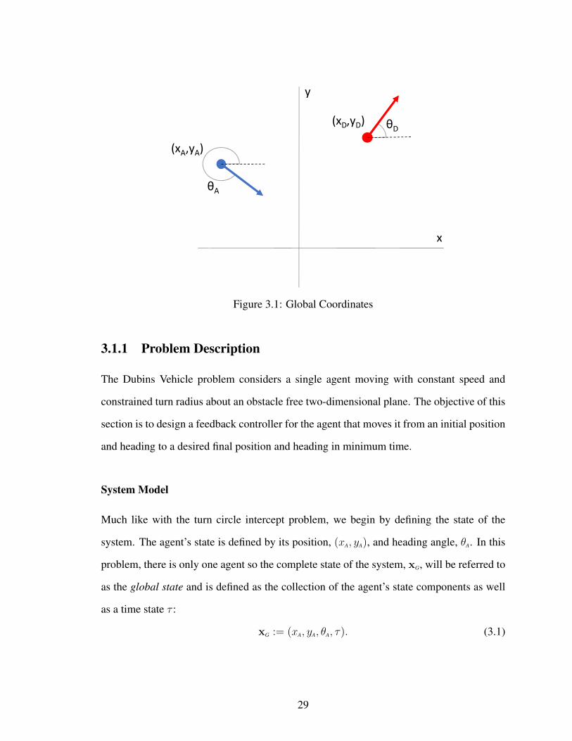
3.1.1 Problem Description
The Dubins Vehicle problem considers a single agent moving with constant speed and
constrained turn radius about an obstacle free two-dimensional plane. The objective of this
section is to design a feedback controller for the agent that moves it from an initial position
and heading to a desired final position and heading in minimum time.
System Model
Much like with the turn circle intercept problem, we begin by defining the state of the
system. The agent’s state is defined by its position, (xA, yA), and heading angle, θA. In this
problem, there is only one agent so the complete state of the system, xG, will be referred to
as the global state and is defined as the collection of the agent’s state components as well
as a time state τ :
xG := (xA, yA, θA, τ). (3.1)
29

ψ
ψDAgent
Desired State
α
α
AD
d
(x,y)
Figure 3.2: Relative Coordinates
The system dynamics xG := f(xG, u) are defined by the following system of ordinary
differential equations:
xA := v cos(θA)
yA := v sin(θA)
θA := ρu
τ := 1,
where the constant v > 0 is the agents’s speed, and ρ > 0 is the agents’s turning rate.
The agent controls its heading through u ∈ [−1, 1]. The desired state is defined as xD :=
(xD, yD, θD) where xD, yD, and θD are parameters that define the desired state’s position and
heading. Figure 3.1 illustrates the agent and a desired state in the two-dimensional x-y
plane. It is important to note that the desired position and heading are constant parameters
that do not change during the course of the simulation.
We will now introduce a second coordinate system which will represent the location
of the agent and desired state relative to the location of the agent. This representation
will allow us to reduce the number of dimensions in later analysis as well as represent the
terminal conditions in a more concise manner. This new coordinate system will be referred
to as the relative coordinate system. The state of the system in relative coordinates xR is
30

Position Buffer
Heading
θ
(x , y)
β
Angle Buffer
dB
(a) Agent’s Buffer Zone
Angle Buffer
Position Buffer
Heading
θD
(xD , yD)
γ dB
(b) Desired State’s Buffer Zone
Figure 3.3: Buffer Zones
defined as
xR := (d, ψ, ψD, τ), (3.2)
where the state d represents the distance between the agent and the desired state. The
angle ψ represents the agents’s relative heading angle and ψD represents the desired state’s
relative heading angle. Both angles are measured counter clockwise from the line segment−−→AD. Just as in the global coordinate system, we also include a time state τ . The relative
coordinate system is depicted graphically in Figure 3.2.
Terminal Conditions
In the Dubins Vehicle problem, termination is achieved when the agent’s state is exactly
equal to the desired state. However, for real-world applications, there will always be a
small amount of error between the current state and the desired state. Additionally, the evo-
lutionary algorithm may generate candidate controllers that never reach the desired state.
Therefore, we consider three possible terminal conditions; successful arrival, maximum
distance reached, and maximum time reached.
Terminal region X1 represents the situation where the agent has reached the desired
31

Agent
Desired State
Figure 3.4: Terminal Condition X1 Example
state as shown in Figure 3.4. In this situation, two distinct criteria have been met. First, the
desired state is within the buffer zone of the agent (represented by the green region in front
of the agent). Second, the agent is within the buffer zone of the desired state (represented by
the red region behind the desired state). Using these criteria, the set of states representing
successful navigation is defined as
X1 := {xR ∈ R7|d < db, cos(ψ) ≥ cos(β),
cos(ψD) ≥ cos(γ)},
where db is a positive constant defining the distance buffer and β and γ are positive con-
stants defining the angle buffers. We can see that if db = β = γ = 0 then the termination
condition can only be met when the agent’s state is exactly equal to the desired state. So
by setting dc, β, and γ to small nonzero values, we can create a small region around the
desired state that the agent can enter to terminate the simulation. The smaller we make
these constants, the closer X1 is to the actual Dubins Vehicle terminal region.
In the cases when the agent implements a control that does not reach the desired state,
we need alternative termination conditions. Terminal region X2 represents the scenario in
32

which the agent reaches a maximum separation distance, dmax, from the desired state.
X2 := {xR ∈ R7|d > dmax}
This prevents the agent from straying too far from the desired position. The case in which
the maximum time tmax is reached is contained in terminal region X3.
X3 := {xR ∈ R7|τ > tmax}
Together, these termination conditions ensure that the simulation will end regardless of the
controller implemented. We define the terminal state as xf = xR(tf ), where the terminal
time, tf , is defined as the moment the relative state of the system falls into the set XT :=
X1 ∪X2 ∪X3
Game Utility
The agents’s utility function, U(u(x);x0,d), consists of a terminal value function φ(xf )
and a time reward as shown in the following equation.
U(u(x);x0) := w1φ(xf ) + w2(tmax − τf ), (3.3)
The terminal value function φ(xf ) is defined as
φ(xf ) :=
c1 xf ∈ X1
c2 xf ∈ X2
c3 xf ∈ X3
. (3.4)
The positive constants w1 and w2 are designed to weigh the effects of the terminal value
33

function and time reward on the overall utility. They also include a scaling factor so that the
effect of each term will remain proportional to its maximum. The values used in this thesis
were w1 = 70c1
and w2 = 30tmax
. With these two weights, the terminal value function can
contribute a maximum utility of 70 and the time reward can contribute a maximum utility
of 30 for a total maximum possible utility of 100.
The terminal value function φ(xf ) is designed to reward the agent for reaching the
desired state. In the event the agent is unable to reach the desired state, agents that stay
within the maximum distance until time runs out are favored over agents that exceed the
maximum distance. In general, the preference for these particular termination conditions
is modeled by selecting weight parameters that satisfy c1 > c3 > c2. For this research, we
used the specific values of c1 = 100, c2 = 0, and c3 = 25.
The terminal value function rewards successful navigation to the desired state, but is
not enough to differentiate which controller does it in the shortest amount of time. There-
fore, a time reward is used that is based on the elapsed time to complete the navigation
τf . The less time the agent takes to complete the simulation, the higher the reward given.
Together with the terminal value function, the time reward ensures controllers that perform
fast and efficient navigations to the desired state (like the Dubins Vehicle optimal solution)
are rewarded the maximum utility.
3.1.2 Controller Design
Optimality analysis of games with similar dynamics [19],[3] have shown that only the rel-
ative configuration information is needed when deciding the optimal control. Through the
use of a relative coordinate system, we can design a controller that will only be dependent
on ψ, ψD, and d.
We begin developing this controller by defining the boundaries of the state space. The
two relative angles, ψ and ψD, can be any real number, but these angles are mapped to
their coterminal angles between 0 and 2π by applying the modulo function. This operation
34

exploits the periodic nature of angles and reduces the range of the state space in those
dimensions to a finite region. The distance d, as defined in Section 3.1.1, is bounded
between 0 and dmax. Combining these ranges implies that all the admissible values of our
state space can be represented in a finite three dimensional subspace: XC = {0 ≤ ψ ≤
2π, 0 ≤ ψD ≤ 2π, 0 ≤ d ≤ dmax}. We can now divide this space into a grid as defined by
three parameters, ε1, ε2, and ε3. These parameters represent the resolution of the grid in the
ψ, ψD, and d dimensions respectively. With this grid, we can now assign a control value to
each of the cells to create our feedback controller.
Although the control is permitted to be continuous within the range of [−1, 1] as de-
fined in Section 3.1.1, it has been shown in analysis of differential games and optimal
control strategies with similar dynamics [17] that the true optimal control strategy has a
bang-zero-bang structure. We also will show in Section 3.1.5 that the analytic optimal Du-
bins solution also has a bang-zero-bang structure. Bang-zero-bang means that the agent
will only implement a hard right, u = −1; go straight, u = 0; or hard left, u = 1, control.
Therefore, we chose to use discrete control values of either u = -1 (turn right) or u = 1 (turn
left) for our grid. While not explicitly included, the go straight control (0) is realized at the
boundaries between the -1 and 1 regions [20, 21]. Figure 3.5 shows an example of a control
grid with resolution of ε1 = ε2 = ε3 = 4. The regions in blue represent a control value of
-1 (turn right) and the regions in yellow represent a control value of +1 (turn left). This grid
can now be used as a feedback controller that has a defined control for every admissible
input state.
We can parametrize the controller using the three dimensional ε1 × ε2 × ε3 matrix u:
u = (ui,j,k)
35

d
ψ
ψD
00 02π
2π
dmax
Figure 3.5: Example of a 4x4x4 Grid Controller
for
i ∈ Z : 1 ≤ i ≤ ε1
j ∈ Z : 1 ≤ j ≤ ε2
k ∈ Z : 1 ≤ k ≤ ε3.
A control can then be selected from this matrix in a look-up-table type manner. Given a
relative state x and control matrix u, the control is defined as
u(x;u) = ua,b,c,
36

1 1 1 −1
1 1 −1 1
1 −1 −1 1
−1 1 −1 −11 −1 1 −1
−1 1 1 −1
1 −1 1 1
1 −1 1 11 −1 1 −1
1 1 −1 1
1 1 −1 1
−1 1 −1 −1−1 1 −1 −1
−1 1 1 −1
1 −1 −1 1
1 −1 1 −1
Figure 3.6: Matrix form of the 4x4x4 Grid Controller in Figure 3.5
for
a = floor
(ε1 [mod(ψ, 2π)]
2π
)+ 1
b = floor
(ε2 [mod(ψD, 2π)]
2π
)+ 1
c = floor
(ε3d
dmax
)+ 1
where ψ, ψD and d are the relative state variables at x and mod(a, b) is the remainder of
ab
(modulo operation). The matrix form of the illustrative example in Figure 3.5 is shown
in Figure 3.6. By using this approach, a control strategy can be completely defined by a
control matrix u. This parameterization will allow us to use an evolutionary algorithm to
evolve u and optimize our agent’s controller for time.
37

3.1.3 Evolutionary Architecture
To begin the EA, a population of N candidate agent controllers is created to serve as gen-
eration 0, G0 = {u1,u2, . . . ,uN} where ui represents the control matrix as described in
the previous section for controller i of the current generation. Each cell in ui is initialized
randomly with either a 1 or -1. After generating the initial population, the evolutionary
algorithm will go through the following steps to create the next generation G1.
• Evaluate Population at Given Initial Conditions
• Assign Fitness Based on Performance
• Create Next Generation Through Mixing and Mutation
These steps will repeat, creating a new generation each time until the algorithm completes
a predefined number of generations, stopping at Gf .
Evaluation
Each candidate controller, ui, is evaluated starting in p different initial conditions. We
will define the set of p initial conditions (represented in relative coordinates) as X0 :=
{x0,1,x0,2, . . . ,x0,p}. The initial conditions used in this paper are summarized in Figure
3.7. The desired state is held constant at the origin with a heading of zero and the agent is
moved around on concentric rings of varying radius from the desired position. These initial
conditions can be represented as:
X0 := {(ψ, ψD, d)|∀ψ ∈ ψ, ψD ∈ ψD, d ∈ d}
38

x
y
Figure 3.7: Initial Conditions
for
ψ =
{n
2π
5| n ∈ Z : 0 ≤ n ≤ 4
}ψD =
{p
2π
5| p ∈ Z : 0 ≤ n ≤ 4
}d =
{1 +m
9
4| m ∈ Z : 0 ≤ m ≤ 4
}.
This results is a total of 125 initial conditions. This collection of initial conditions is de-
signed to thoroughly test the candidate controller and ensure that the evolved solutions are
effective from many different initial conditions.
39

Fitness
The evaluation of candidate control matrix ui initiated at x0,k provides a utility which we
will refer to as a sub-fitness. This sub-fitness is defined as
fs(ui,x0,k) := U(u(x;u)i),x0,k). (3.5)
The cumulative fitness of an agent, fc, represents its average sub-fitness from all the given
initial conditions, where
fc(ui;X0) :=1
125
125∑k=1
fs(ui;x0,k). (3.6)
The goal of this optimization problem is to maximize the utility achieved by the agents’s
control matrix u in the set of initial conditions X0:
maxu
fc(ui;X0). (3.7)
Creating Next Generation
After the current generation Gi has been evaluated and every candidate controller has a
cumulative fitness assigned to them, the next generation Gi+1 is created. As defined in the
beginning of this section, G0 contains N candidate controllers. In order to maintain consis-
tency, each generation is held to the same constant number of N candidate controllers. The
composition of the new N players is shown in Figure 3.8 and is described in the following
sub-sections.
40

Fitn
ess
Old Gen Next GenElite
Fitness Based
CrossingMutation
5%
95%
Figure 3.8: Population Generation Method
Copies of Elite Controllers
The set of elite controllers is comprised of the candidate controllers with cumulative fitness
in the top 5% of the generation. These candidate controllers are passed on to the next
generation with no mutation. By segregating these elite controllers and passing them on
between the generations unaltered, we can guarantee that the maximum cumulative fitness
will never go down.
Fitness-Based Crossing of Two Controllers
The remaining 95% of the next generation is filled with the offspring from fitness-based
crossing. The likelihood that a candidate controller is selected for crossing increases pro-
portionally to its relative fitness with respect to the rest of the population. More specifically,
for any given candidate controller un of cumulative fitness fc(un;X0) the probability of se-
lection p is,
p =fc(un;X0)∑Ni=1 fc(ui;X0)
41

Once two parent candidate controllers (P1 and P2) are selected, they are mixed using the
following method. Two points (hereby referred to as split points) s1 and s2 are randomly
selected in the ε1 × ε2 × ε3 cube. The child is created by comparing the magnitude of the
distance from each matrix index (i, j, and k) to these split points. Matrix indices closer to
split point s1 will be filled with P1’s control value at that index and indices closer to split
point s2 will be filled with P2’s control value at that index.
Ci,j,k =
P1i,j,k |[i, j, k]− s1| ≤ |[i, j, k]− s2|
P2i,j,k |[i, j, k]− s1| > |[i, j, k]− s2|
The resulting child C is then passed through a mutation function where each matrix index
Ci,j,k has a pm chance of mutating. The mutation chance pm is defined as,
pm =1
ε1ε2ε3.
Once selected for mutation, the mutation is performed by flipping the control value. So for
example if C1,4,2 = −1 is selected for mutation, it would become C1,4,2 = 1.
42

3.1.4 Results and Analysis
The results in this section were obtained by evolving a population of 100 controllers over
5000 generations with the following simulation parameters.
Control Grid Resolution: ε1 = ε2 = ε3 = 15
Buffer Zone Angle: β = γ = π/2
Buffer Zone Distance: dB = 1
Terminal Value Fitness Weight: w1 = 70
Time Reward Fitness Weight: w2 = 30
In order to better evaluate these results, the analytically optimal Dubins Vehicle solution,
solved by L. E. Dubins [1], will be used as a benchmark. This will allow us to see if the
evolutionary algorithm is actually approximating the underlying optimal solution.
3.1.5 Dubins Vehicle Optimal Solution
The Dubins optimal solution can be geometrically described as connecting circles tangent
to the agent, to circles tangent to the desired location. The radius of these circles is defined
by the constant turn rate ρ. There are two different ways of connecting these tangent circles;
turn-straight-turn (TST) solutions, and turn-turn-turn (TTT) solutions. An example of a
TST solution is shown in Figure 3.9. The blue dotted circles are the circles tangent to the
agent. The red dashed circles are the circles tangent to the desired state. The thick magenta
line shows the trajectory taken from the agent starting location to the desired state. TST
solutions are used for all initial conditions that have distance to the desired state greater
than or equal to 4rmin, where rmin is the radius of the circle made with the given constant
turn rate ρ. This type of solution can also appear when the distance to the desired state is
43

-4 -2 0 2 4 6 8 10 12 14
-6
-4
-2
0
2
4
6
Turn-Straight-Turn
Figure 3.9: Turn-Straight-Turn (TST) Solution
-4 -2 0 2 4 6 8
-2
-1
0
1
2
3
4
5
6
7
Turn-Turn-Turn
Figure 3.10: Turn-Turn-Turn (TTT) Solution
44

500 1000 1500 2000 2500 3000 3500 4000 4500 5000
Generations
0
10
20
30
40
50
60
70
80
90
100
Fitn
ess
Evolution of Fitness of Population
Max FitnessMean Fitness
Figure 3.11: Fitness Throughout the Evolution
less than 4rmin, however in this region it is sometimes outperformed by a turn-turn-turn
solution. An example of a TTT solution is shown in Figure 3.10. These solutions appear
when the distance between the players is less than 4rmin. As can be seen, in these solutions
the agent uses a connecting third circle that is tangent to both the agents’s tangent circle
and the desired state’s tangent circle. Together, these two solution types completely define
the Dubins Vehicle optimal solution and can be used to find the path of shortest travel time
for a turn constrained agent with constant velocity.
Analysis of Evolution
We will now examine the performance of the evolutionary algorithm. Figure 3.11 shows
the maximum and average cumulative fitness in each generation over the 5000 generations
of evolution. The fitness follows a logarithmic shape, where the majority of the fitness
increase happens from generation 1 to generation 500. Figure 3.12 shows a close up of
this region with the number of successful navigations overlaid. One can see that the fitness
increases in sharp jumps that largely correspond with increases in the percent of successful
45

50 100 150 200 250 300 350 400 450 500
Generations
0
10
20
30
40
50
60
70
80
90
100
Fitn
ess
0
10
20
30
40
50
60
70
80
90
100
Per
cent
of N
avig
atio
ns E
ndin
g S
ucce
ssfu
lly
Evolution of Fitness of Population
Max FitnessMean FitnessSuccessful Navigations
G145G481G46
G25
G1
G16
Figure 3.12: Fitness and Success from Gen 1 to 500
navigations. By generation 481, the evolutionary algorithm has developed a controller that
is able to successfully navigate to the desired state from all of the tested initial conditions.
Figure 3.13 shows the remainder of the evolution (generations 500 to 5000). We can
see that the fitness still increases even though the rate of successful navigations stays at 100
percent. This continued fitness increase is a result of the time bonus in our utility function
shown in Equation 3.3. This part of the evolution focused on optimizing the trajectories
for time while maintaining the 100 percent success rate. The evolutionary algorithm was
able to maintain the 100 percent success rate due to the use of elitism. Elitism ensures that
the maximum fitness never goes down from one generation to the next. By weighing the
terminal value score (w1 = 70) much higher than the time bonus (w2 = 30), we created a
strong bias against reducing the number of successful navigations from one generation to
the next. The marginal fitness improvements from the time bonus were never enough to
outweigh the loss of a successful navigation. The only way for the evolutionary algorithm
to increase the overall fitness, was for it to find controllers that scored a higher time bonus
without disturbing the 100 percent capture rate. With these high level fitness trends in
46

500 1000 1500 2000 2500 3000 3500 4000 4500 5000
Generations
84
86
88
90
92
94
96
98
100
Fitn
ess
84
86
88
90
92
94
96
98
100
Per
cent
of N
avig
atio
ns E
ndin
g S
ucce
ssfu
lly
Evolution of Fitness of Population
Max FitnessMean FitnessSuccessful Navigations
G1698
G5000
G730
Figure 3.13: Fitness and Success Gen 500 to 5000
mind, we can now examine the performance of the evolved controllers at multiple points of
interest throughout the evolution. These points are chosen to highlight some fitness leaps
in the evolutionary process and have been marked on Figures 3.12 and 3.13.
To begin, we will take a more detailed look at the evolution of successful navigations
in generations 1 through 481. Figure 3.14 shows a summary of the successful captures
at the marked generations. Similar to Figure 3.7, each small blue circle represents the
(x, y) location of five initial conditions (one for each agent heading). If any of these five
initial conditions end in a successful navigation, a line extending out from the point in the
direction of the initial condition’s heading is drawn. The arcs at the end of these lines are
a visual aid to help one more easily see what percent of initial conditions end in success
from a particular point. When all five initial conditions at a point end successfully, the arcs
will form a full circle. Using this information we can see where the successful navigations
are concentrated and how they evolved.
Starting with Figure 3.14a, one can see that there are only a few initial conditions
47

-10 -8 -6 -4 -2 0 2 4 6 8 10
x
-10
-8
-6
-4
-2
0
2
4
6
8
10
y
(a) Generation 1
-10 -8 -6 -4 -2 0 2 4 6 8 10
x
-10
-8
-6
-4
-2
0
2
4
6
8
10
y
(b) Generation 16
-10 -8 -6 -4 -2 0 2 4 6 8 10
x
-10
-8
-6
-4
-2
0
2
4
6
8
10
y
(c) Generation 25
-10 -8 -6 -4 -2 0 2 4 6 8 10
x
-10
-8
-6
-4
-2
0
2
4
6
8
10
y
(d) Generation 46
-10 -8 -6 -4 -2 0 2 4 6 8 10
x
-10
-8
-6
-4
-2
0
2
4
6
8
10
y
(e) Generation 145
-10 -8 -6 -4 -2 0 2 4 6 8 10
x
-10
-8
-6
-4
-2
0
2
4
6
8
10
y
(f) Generation 481
Figure 3.14: Summary of Successful Captures
that end in success and they are concentrated in the region above the desired location.
Moving on to Figure 3.14b, we can see that many new successful initial conditions have
been added. There are however some instances were an initial condition that was successful
in generation 1 is no longer successful in generation 16. While this may seem like negative
behavior, it is in fact a result of our fitness function. The evolutionary algorithm traded
a few old successful navigations for a larger number of new successful navigations which
resulted in an overall increase in fitness. This trend continues through Figures 3.14c and
3.14d, with the evolutionary algorithm adding many new successful navigations at the cost
of only a few previously successful initial conditions. By generation 145 there are only
seven initial conditions that do not end successfully. At this point the evolution slows
down, and it takes 336 more generations to develop a controller that is able to reach the
desired state from all of the tested initial conditions.
In order to get a better idea of how the trajectories evolved, we will now examine the
48

-15 -10 -5 0 5 10 15
x
-15
-10
-5
0
5
10
15
y
(a) Initial Condition 1
-15 -10 -5 0 5 10 15
x
-15
-10
-5
0
5
10
15
y
(b) Initial Condition 2
-15 -10 -5 0 5 10 15
x
-15
-10
-5
0
5
10
15
y
(c) Initial Condition 3
-15 -10 -5 0 5 10 15
x
-15
-10
-5
0
5
10
15
y
(d) Initial Condition 4
Figure 3.15: Generation 1
-15 -10 -5 0 5 10 15
x
-15
-10
-5
0
5
10
15
y
(a) Initial Condition 1
-15 -10 -5 0 5 10 15
x
-15
-10
-5
0
5
10
15
y
(b) Initial Condition 2
-15 -10 -5 0 5 10 15
x
-15
-10
-5
0
5
10
15
y(c) Initial Condition 3
-15 -10 -5 0 5 10 15
x
-15
-10
-5
0
5
10
15
y
(d) Initial Condition 4
Figure 3.16: Generation 25
-15 -10 -5 0 5 10 15
x
-15
-10
-5
0
5
10
15
y
(a) Initial Condition 1
-15 -10 -5 0 5 10 15
x
-15
-10
-5
0
5
10
15
y
(b) Initial Condition 2
-15 -10 -5 0 5 10 15
x
-15
-10
-5
0
5
10
15
y
(c) Initial Condition 3
-15 -10 -5 0 5 10 15
x
-15
-10
-5
0
5
10
15
y
(d) Initial Condition 4
Figure 3.17: Generation 145
performance of the controller with the highest cumulative fitness at several of our marked
generations. The following set of figures show the trajectories taken from a sample of four
initial conditions. The thick blue line shows the path taken by the agent controlled with
the controller of highest cumulative fitness in the generation. If it is solid, it indicates a
successful navigation. If it is dashed, it indicates an unsuccessful navigation. The thin
black dashed line shows the Dubins Vehicle optimal solution. The red drawing in the
middle represents the desired state’s location, heading, and buffer region behind it.
To begin, Figure 3.15 shows the trajectory taken by an agent using the controller with
49

-15 -10 -5 0 5 10 15
x
-15
-10
-5
0
5
10
15
y
(a) Initial Condition 1
-15 -10 -5 0 5 10 15
x
-15
-10
-5
0
5
10
15
y
(b) Initial Condition 2
-15 -10 -5 0 5 10 15
x
-15
-10
-5
0
5
10
15
y
(c) Initial Condition 3
-15 -10 -5 0 5 10 15
x
-15
-10
-5
0
5
10
15
y
(d) Initial Condition 4
Figure 3.18: Generation 481
-15 -10 -5 0 5 10 15
x
-15
-10
-5
0
5
10
15
y
(a) Initial Condition 1
-15 -10 -5 0 5 10 15
x
-15
-10
-5
0
5
10
15
y
(b) Initial Condition 2
-15 -10 -5 0 5 10 15
x
-15
-10
-5
0
5
10
15
y
(c) Initial Condition 3
-15 -10 -5 0 5 10 15
x
-15
-10
-5
0
5
10
15
y
(d) Initial Condition 4
Figure 3.19: Generation 1698
-15 -10 -5 0 5 10 15
x
-15
-10
-5
0
5
10
15
y
(a) Initial Condition 1
-15 -10 -5 0 5 10 15
x
-15
-10
-5
0
5
10
15
y
(b) Initial Condition 2
-15 -10 -5 0 5 10 15
x
-15
-10
-5
0
5
10
15
y
(c) Initial Condition 3
-15 -10 -5 0 5 10 15
x
-15
-10
-5
0
5
10
15
y
(d) Initial Condition 4
Figure 3.20: Generation 5000
50

highest cumulative fitness in generation 1. As can be seen in Figures 3.15a, 3.15b, and
3.15d, most of the trajectories randomly wander around the space until they either exceed
the maximum distance or time runs out. Figure 3.15c however shows a trajectory that
actually seems to resemble the Dubins Vehicle optimal solution. Since this is generation
1, no evolution has yet taken place and this is simply the result of a randomly generated
control matrix.
A few generations later in generation 25, we can see that while three of our sample
initial conditions are still unsuccessful, initial condition 3 (Figure 3.16c) has tightened its
final turn and is now very close to the Dubins Vehicle optimal solution.
Moving on to generation 145 (Figure 3.17), we can see that all four of our sample
initial conditions now result in successful navigation. However just because they end suc-
cessfully, does not mean that they do so in a time effective manner. For example initial
conditions 1 and 4 (Figures 3.17a and 3.17d respectively) show trajectories that take a very
indirect path. We can see however in initial condition 4, that while it did end up taking a
long path, it seems to have narrowly missed the desired state on its initial approach and as a
result had to loop around. One small change in the control could allow this initial condition
to capture on its initial approach which would greatly improve the fitness.
By generation 481, we can see that this small change did indeed happen, and initial
condition 4 now captures on its initial approach (Figure 3.18d). In addition to that we can
see that the change did not disturb the performance of initial conditions 2 and 3. Looking
back to figure 3.14f, we can see that from this point onward, all of the initial conditions end
successfully and thus the evolutionary algorithm now improves time performance without
degrading the 100% capture rate.
In generation 1698, (Figure 3.19) we can see that initial conditions 2, 3, and 4 closely
approximate the Dubins Vehicle optimal solution and thus improved their time score. In
fact they are overlapping the optimal solution for the majority of their trajectory. How-
ever the controller still is unable to match the turn-turn-turn optimal solution from initial
51

condition 1.
The final set of results in Figure 3.20 show the performance of the best controller in
generation 5000. This is the best controller evolved by the evolutionary algorithm. As can
be seen, in Figure 3.20a, the best controller has developed a turn-turn-turn solution and
now very closely matches the Dubins Vehicle optimal solution from all four of our sample
initial conditions.
Overall, these results show that the evolutionary algorithm was able to gradually in-
crease fitness through incremental improvements in the controller’s performance. The use
of elitism and the specific weights in our utility function allowed the algorithm to begin
by focusing on successful navigations and then transition to optimizing the trajectories for
time. While we only examined four sample initial conditions, the same analysis can be
done for any of the 125 initial conditions and similar trends will be found. The trajectories
begin by randomly moving around the space and gradually improve their performance until
they almost completely overlap the Dubins Vehicle optimal solution.
Results of Evolutionary Algorithm
The end result of the evolutionary algorithm is the controller with highest cumulative fitness
in generation 5000 (hereby referred to as the best evolved controller). Figure 3.21 shows
the trajectories taken by the best evolved controller starting from a sample of five initial
conditions. The thick blue lines show the agent’s trajectory and the thin dashed black lines
represent the Dubins Vehicle optimal trajectory. We can see that the resulting best controller
was able to approximate the Dubins Vehicle optimal solution very closely, developing both
TST and TTT solutions.
Figure 3.22 shows a close up of initial condition A. The Dubins Vehicle optimal so-
lution in this case is a TTT solution. The best evolved controller also implements a TTT
solution that only slightly deviates from the optimal trajectory. Figure 3.23 shows a close
52

Figure 3.21: Performance of Best Controller from Trained IC
up of initial condition E. As can be seen, the Dubins Optimal trajectory here is a TST so-
lution. Once again, the best controller is able to match this solution type with only slight
variations in the trajectory.
The fact that both TTT and TST solutions emerged from the evolutionary algorithm
is important because it shows the ability of the algorithm to find the small performance
differences between the two solutions and apply them in the correct situations. Addition-
ally, as described in section 3.1.2, going straight was not explicitly included in our control
space. The agent could only turn left or right. So in order for evolutionary algorithm to
develop controllers that have these straight sections, it had to accurately place the bound-
aries between the left and right regions so that it could switch between them as it moved
through the state space. As a result of rapidly switching between left and right, the overall
trajectory appears to be straight.
53

-4 -2 0 2 4 6
x
-2
0
2
4
6
8y
A
Figure 3.22: Evolved TTT Solution vs Op-timal TTT Solution -10 -8 -6 -4 -2 0 2
x
-4
-2
0
2
4
6
y
E
Figure 3.23: Evolved TST Solution vs Op-timal TST Solution
Further Analysis
As stated in the introduction, one of the primary advantages of evolving a feedback con-
troller is that it allows our evolved solution to be applied at any admissible initial condition.
If the evolutionary algorithm truly approximates the underlying Dubins Vehicle optimal
controller, it should be able to translate its performance into these new untrained initial
conditions.
In order to test this, we evolved a feedback controller from 216 initial conditions. We
then took the best evolved controller and evaluated it at a set of 10, 000 random untrained
initial conditions. These random initial conditions were generated by uniformly selecting
a value for ψ, and ψD in their admissible ranges (0 ≤ ψ < 2π and 0 ≤ ψD < 2π),
and d in a smaller range to avoid starting too close to the maximum distance terminal
condition (1 ≤ d ≤ dmax
2). From these tests, we found that the best evolved controller was
able to successfully navigate to the desired state from 94.67% of the 10,000 random initial
conditions with an average time to termination of 1.67 times the Dubins Vehicle optimal
solution time.
Figure 3.24 shows some of the random initial conditions that ended successfully. As
54

-15 -10 -5 0 5 10 15
x
-15
-10
-5
0
5
10
15
y
Figure 3.24: Performance from Untrained IC
can be seen, even in these untrained initial conditions, the best controller was able to closely
approximate the Dubins Vehicle optimal solution. By evolving a parameterized feedback
controller with a set of only 216 initial conditions, we were able to develop a solution
that can be applied to the entire continuum of initial conditions and approximate the true
optimal solution 94.67% of the time.
The controller parameterization used in the evolutionary algorithm was a 15x15x15
grid, whereas the true Dubins Vehicle optimal solution exists in continuous space. Figure
3.25 shows an illustrative example of a two-dimensional control space. Figure 3.25a shows
the true continuous boundary between turn left and turn right. When we discretized it as
shown in Figure 3.25b, we can see that the new boundary is quite different from the original
one (shown as the dotted line). The grid restricts where the controller can change its control
and thus will cause deviations from the true optimal solution.
To further illustrate this, Figures 3.26a-c show a slice of the three dimensional control
space at distance d = 7 for three different controllers; the true Dubins Vehicle optimal
55

(a) True Solution (b) Grid Approximation of Solution
Figure 3.25: Example of Grid Parameterization Error
controller, the discretized Dubins Vehicle optimal controller, and the best evolved con-
troller. Starting with the true Dubins Vehicle optimal solution (Figure 3.26a), we can see
that the boundaries between turn left (yellow) and turn right (blue) are quite complicated
with curves and sharp corners. We can discretize this continuous controller and end up
with the boundaries shown in Figure 3.26b. We can immediately see a degradation in the
ability of the controller to accurately represent these boundaries. Moving on to the best
evolved controller (3.26c), we can see that the Dubins Vehicle optimal boundaries are very
poorly represented. There is some resemblance between the two controllers, but in general
the control seems to be much more chaotically distributed.
Looking at these controllers, it would seem that the discretized Dubins controller is
the best possible 15x15x15 approximation of the true underlying solution. Furthermore, it
would seem that the evolved solution is overfit to our tested initial conditions and doesn’t
truly represent the underlying solution. To test this we evaluated all three of these con-
trollers from a sample untrained initial condition. Figures 3.26d-f show the corresponding
trajectories. From these trajectories, one can see that the discretized Dubins controller is
actually unable to reach the desired state and performs much worse than the evolved con-
56

d = 7
0 1 2 3 4 5 6
PsiB
0
1
2
3
4
5
6
Psi
A
(a) Dubins Vehicle OptimalSolution
d = 7
0 1 2 3 4 5 6
PsiB
0
1
2
3
4
5
6
Psi
A
(b) Discretized Dubins VehicleOptimal Solution
d = 7
0 1 2 3 4 5 6
PsiB
0
1
2
3
4
5
6
Psi
A
(c) Evolved Controller
-15 -10 -5 0 5 10 15
x
-15
-10
-5
0
5
10
15
y
(d) Dubins Vehicle OptimalPath
-15 -10 -5 0 5 10 15
x
-15
-10
-5
0
5
10
15
y
(e) Discretized Dubins VehiclePath
-15 -10 -5 0 5 10 15
x
-15
-10
-5
0
5
10
15
y
(f) Evolved Path
Figure 3.26: Evolved vs Discretized Dubins
troller. In fact, when tested from an array of 10,000 initial conditions (similarly to our
evolved controller), this discretized controller was only able to capture 52.30% of the time
with an average time to termination of 5.31 times the Dubins Vehicle optimal solution time.
Ideally, the best possible controller would perfectly represent the true optimal bound-
aries and thus perfectly represent the Dubins Vehicle optimal solution. However, since our
grid parameterization prevented the controllers from accurately representing the bound-
aries, the evolutionary algorithm developed a new solution that closely resembles the per-
formance of the Dubins vehicle optimal solution without accurately representing the cor-
rect boundaries. This is an important result as it shows the flexibility of the evolutionary
algorithm. Given the limitations of the grid parameterization used, we can see that the
evolved controller actually performed quite well. Even with a simple low resolution grid
controller, the evolutionary algorithm was able to develop a solution that approximates the
57

Dubins Vehicle optimal solution 94.67% of the time. In the future, more sophisticated con-
troller representations will be examined in an attempt to better approximate the underlying
boundaries and thus allow us to obtain more accurate solutions.
3.1.6 Impact of Results
In conclusion, we can see that the evolutionary algorithm was able to create a feedback
(closed-loop) controller that closely approximates the Dubins Vehicle optimal solution
from all of our trained initial conditions. Since a feedback controller was used, we were
also able to test the resulting best controller in a wide variety of random untrained initial
conditions. The best evolved controller was able to successfully approximate the Dubins
Vehicle optimal solution in approximately 94.67% of these random initial conditions. By
evolving feedback controllers, one can develop solutions that can be applied to an entire
continuum of initial conditions. In the next section will aim to expand upon this work by
exploring different controller parameterizations that may allow us to better represent the
precise control boundaries of the underlying optimal solution and thus obtain better con-
trollers. In addition to that, we will attempt to use this evolutionary algorithm to solve a
more complex problems in which the optimal solution has not been analytically solved for.
3.2 Pursuit Evasion
The second problem we will examine is the turn-constrained pursuit evasion problem. As
stated in the introduction of this thesis, the goal of creating our EA methodology is so
that we can apply it to problems in which the optimal is not known and hopefully obtain
deployable solutions. This problem does not have an easily derivable analytical solution
and thus will serve as the first real test of our EA. Since there is no optimal to compare to,
our results will be subjectively evaluated based on their performance.
58

3.2.1 Problem Description
The scenario under consideration consists of two players, Player A and Player B, moving
with constant speeds and constrained turn rates about an obstacle-free 2D plane. In the
general case, Player A strives to capture Player B from behind. Simultaneously Player
B attempts to capture Player A while evading capture itself. It is assumed that Player A
possesses superior dynamics such that it is capable of capturing Player B from any initial
condition.
System Model
Player A’s state is defined by its position, (xA, yA), and heading angle, θA. Similarly Player
B’s state is defined by its position, (xB, yB), and heading angle, θB. Figure 3.27 illustrates
these players. The complete state of the system, xG, will be referred to as the global state
and is defined as the collection of the individual agent states as well as a time state τ :
xG := (xA, yA, θA, xB, yB, θB, τ). (3.8)
The system dynamics xG := f(xG, uA, uB) are defined by the following system of ordi-
59

(xB,yB)(xA,yA)
θB
θA
y
x
Figure 3.27: Global Coordinates
nary differential equations:
xA := vA cos(θA) (3.9)
yA := vA sin(θA) (3.10)
θA := ρAuA (3.11)
xB := vB cos(θB) (3.12)
yB := vB sin(θB) (3.13)
θB := ρBuB (3.14)
τ := 1, (3.15)
where the constants vA > 0 and vB > 0 are Player A’s and Player B’s respective speeds.
The constants ρA > 0 and ρB > 0 are Player A’s and Player B’s maximum turn rates. To
fulfill our assumption that Player A has superior dynamics, vA > vB and ρA > ρB. Player
A controls its heading through uA ∈ [−1, 1] while Player B controls its heading through
uB ∈ [−1, 1]. In addition to their state, each player has a field of view and capture region
defined by the positive constant angles β and γ, respectively as shown in Figure 3.28. These
angles will be used to define the termination condition of the pursuit.
60
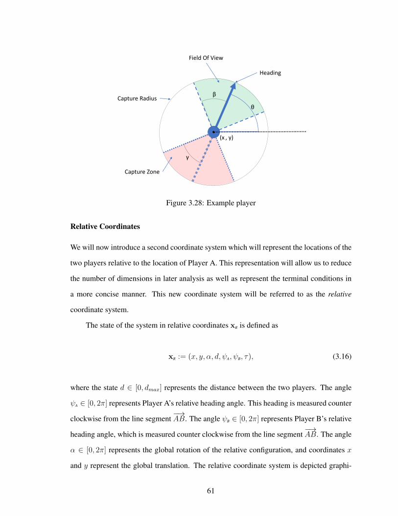
Field Of View
Capture Zone
Capture Radius
Heading
θ
(x , y)
γ
β
Figure 3.28: Example player
Relative Coordinates
We will now introduce a second coordinate system which will represent the locations of the
two players relative to the location of Player A. This representation will allow us to reduce
the number of dimensions in later analysis as well as represent the terminal conditions in
a more concise manner. This new coordinate system will be referred to as the relative
coordinate system.
The state of the system in relative coordinates xR is defined as
xR := (x, y, α, d, ψA, ψB, τ), (3.16)
where the state d ∈ [0, dmax] represents the distance between the two players. The angle
ψA ∈ [0, 2π] represents Player A’s relative heading angle. This heading is measured counter
clockwise from the line segment−→AB. The angle ψB ∈ [0, 2π] represents Player B’s relative
heading angle, which is measured counter clockwise from the line segment−→AB. The angle
α ∈ [0, 2π] represents the global rotation of the relative configuration, and coordinates x
and y represent the global translation. The relative coordinate system is depicted graphi-
61

ψA
ψB
Player A
Player B
α
α
AB
d
(x,y)
Figure 3.29: Relative Coordinates
cally in Figure 3.29. Just as in the global coordinate system, we also include a time state
τ .
The global and relative coordinate systems are related through the following equa-
tions:
x := xA (3.17)
y := yA (3.18)
α := arctan
(yB − yA
xB − xA
)(3.19)
d :=√
(xB − xA)2 + (yB − yA)2 (3.20)
ψA := θA − α (3.21)
ψB := θB − α. (3.22)
Terminal Conditions
The terminal time, tf , is defined as the moment the relative state of the system falls into
one of the following terminal regions. We define the terminal state as xf = xR(tf ).
62

X1 := {xR ∈ R7|d < dc, cos(ψA) ≥ cos(βA),
cos(ψB) ≥ cos(γB)}(3.23)
X2 := {xR ∈ R7|d < dc, cos(ψA) ≤ − cos(γA),
cos(ψB) ≤ − cos(βB)}(3.24)
X3 := {xR ∈ R7|d ≥ dmax} (3.25)
X4 := {xR ∈ R7|τ ≥ tmax} (3.26)
where dc is a positive constant defining the capture radius.
Each of these regions corresponds to one of four different termination conditions. X1
represents the region in which Player A captures Player B as shown in Figure 3.30a. In this
situation, three distinct criteria have been met. First, the players have entered inside of the
capture distance. Second, Player B is within the field of view of Player A (represented by
the green region in Player A’s circle). Third, Player A is within the capture zone of Player
B (represented by the red region in Player B’s circle). Conversely, region X2 represents the
region in which Player B captures Player A as shown in Figure 3.30b. This event simply
reverses the roles of Player A and Player B so that Player A is in the field of view of Player
B and Player B is in the capture zone of Player A. The scenario in which the two players
reach a maximum separation distance dmax is represented by X3, and the case in which the
maximum time tmax is reached is represented by X4.
Game Utility
Player A’s utility function, UA(uA(x), uB(x);x0), consists of a terminal value function
φ(xf ) and a time penalty:
63

Player A
Player B
(a) Player A captures Player B
Player A
Player B
(b) Player B captures Player A
Figure 3.30: Example of capture conditions
UA(uA(x), uB(x);x0) := w1φ(xf )− w2τf , (3.27)
where the terminal value function φ(xf ) is defined as
φ(xf ) :=
c1 xf ∈ X1
c2 xf ∈ X2
c3 xf ∈ X3
c4 xf ∈ X4
(3.28)
The positive constants w1 and w2 are designed to weigh the effects of the terminal value
function and time penalty on the overall utility. The values used in this research were
designed to favor a successful end condition over an efficient path. To model these prefer-
ences, we used w1 = 60 and w2 = 40.
The terminal value function φ(xf ) is designed to reward Player A for capturing Player
B, and discourage Player A from being captured by Player B. In the event of no capture,
players that stayed within the maximum distance until time ran out should be awarded more
points and favored over the players that retreated. To model these preferences we used the
specific values of c1 = 100, c2 = 0, c3 = 10, and c4 = 25.
The terminal value function rewards successful capture, but is not enough to differ-
64

entiate which capture strategy is better than another capture strategy. Therefore, a time
penalty is added that is based on the elapsed time to complete the pursuit τf . The more
time Player A takes to complete the chase, the higher the penalty incurred. Together with
the terminal value function, the time penalty ensures players that perform fast and efficient
captures are rewarded the maximum utility.
3.2.2 Controller Design
Although the control for Player A and Player B is allowed to be continuous within the range
[−1, 1] as defined in Section 3.2.1, it has been shown in analysis of differential games and
optimal control strategies with similar dynamics [17] that the true optimal control strategy
has a bang-zero-bang structure. This means that the players will only implement a hard
right, u = −1; go straight, u = 0; or hard left, u = 1, control. Therefore, we chose to
represent the feedback control strategy for each agent using a nearest neighbor switching
controller (NNSC) [20, 21].
We begin developing this controller by defining the concept of anchor points, ai :=
{xi, ui}, where xi is the location of the anchor point within the state space and ui ∈
{−1, 0, 1} is the discrete control implemented when near that anchor point. Given a set
of anchor points S = {a1, a2, . . . , an}, we define the NNSC as
u(x;S) = ui, (3.29)
where i is the index that identifies the nearest anchor point to the current state x: i =
arg mini |x − xi|. By using this anchor point approach, a player’s entire control strat-
egy is completely defined by its set of anchor points S. The set of anchor points can be
65

Figure 3.31: Three Anchor Points Subdividing a 2D Space
parametrized using an n× (m+ 1) matrix ma:
ma =
x1 u1
......
xn un
, (3.30)
where n is the number of anchor points within the set andm is the number of dimensions of
the state space. Each row of the matrix represents one anchor point. The first m elements
of the ith row parameterize xi and the last element parameterizes ui.
This control scheme divides the state space into regions of discrete control. An illus-
trative two-dimensional example is depicted in Figure 3.31. In this specific example, the
space is subdivided into three distinct regions. If the current state was in the red region,
then the control would be go full left; if the state was in the green region, the control would
be go full right; if the state was in the blue region, then the control would be go straight.
As defined in Section 3.2.1, the two-agent problem exists within a seven-dimensional
state space. However, optimality analysis of games with similar dynamics [19, 3] has
shown that only the relative configuration information is needed when deciding the optimal
control. Through the use of a relative coordinate system as defined in (3.17)-(3.22), we can
utilize only the relative dimensions, d, ψA, and ψB, of the state space to reduce the controller
space to three dimensions. Although we will simulate the global rotation α and translation,
66

x and y, the controller will only be dependent on d, ψA, and ψB.
Since two of the three dimensions used in our control are angular, one more step is
taken in order to better represent the distances between anchor points. This step maps d,
ψA and ψB to the three Cartesian axes xT, yT, zT . To do this we used a toroidal coordinate
system with mapping defined by the equations below where κ is a constant that defines the
radius of the circle in the middle of the toroid.
xT := cos(ψA) [κ+ (dmax − d) cos(ψB)] (3.31)
yT := sin(ψA) [κ+ (dmax − d) sin(ψB)] (3.32)
zT := (dmax − d) sin(ψB) (3.33)
The position of the anchor points is represented using this three-dimensional toroidal coor-
dinate system.
3.2.3 Evolutionary Architecture
The focus of this section is to create an evolutionary algorithm that is able to develop ef-
fective feedback control strategies for Player A in response to an aggregate population of
representative strategies for Player B. The evolutionary algorithm needs to be able to pre-
serve players with good performance while still maintaining a diverse enough population
to avoid local optima and effectively search the space. It also needs to make meaningful
changes to the players between generations in order to progress towards an optimal solu-
tion.
To begin, a population of N candidate Player A controllers is created to serve as
generation 0, G0 = {SA1, SA2, . . . , SAN} where SAi represents the set of anchors defining
a candidate NNSC as described in Section 3.2.2. Each SAi is initialized with one anchor
point that is randomly placed somewhere inside of the 3D bounded toroid space.
67

After generating the initial population, the evolutionary algorithm will go through the
subsequent steps to create the next generation G1.
• Evaluate Population vs Benchmark Competition
• Assign Fitness Based on Performance
• Create Next Generation Through Mixing and Mutation
These steps will repeat, creating a new generation each time until the algorithm completes
a predefined number of generations, stopping at Gf .
Competition
Each candidate controller, SAi, is evaluated against a set of m Player B benchmark strate-
gies using p different initial conditions. These predefined Player B benchmark strategies
are representative of the range of behaviors Player A may encounter when deployed. We
will refer to this collection of Player B strategies as the benchmark set, SB. In this paper,
the benchmark set consists of five different strategies, SB = {SB1, SB2, . . . , SB5}. Each of
these strategies represents a qualitatively different type of behavior. Strategy SB1 models
an always go straight behavior in which Player B always implements uB = 0. Its matrix
representation is defined as m1 := (0, 0, 0, 0). Strategy SB2 represents an always turn right
behavior and its matrix representation is defined as m2 := (0, 0, 0,−1). Strategy SB3 is
an always turn left behavior with a matrix representation of m3 := (0, 0, 0, 1). Strategy
SB4 models a fleeing behavior in which Player B attempts to always turn away from the
attacker. The fleeing parameterization is defined as
m4 :=
0 dmax 0 1
0 −dmax 0 −1
. (3.34)
68

Lastly, strategy SB5 represents an aggressive strategy in which Player B always attempts to
turn towards the attacker with a parameterization of
m5 :=
0 dmax 0 −1
0 −dmax 0 1
. (3.35)
We will define the set of p initial conditions (represented in relative coordinates) as
X0 := {x0,1,x0,2, . . . ,x0,p}. In this paper, there are four specific initial conditions:
x0,1 := (−50, 0, 0, 100, 0, π, 0) (3.36)
x0,2 := (−50, 0, 0, 100, π, 0, 0) (3.37)
x0,3 := (−50, 0, 0, 100, 0, 0, 0) (3.38)
x0,4 := (−50, 0, 0, 100, π, π, 0) (3.39)
The initial condition x0,1 represents a starting position where both players are facing
each other. The initial condition x0,2 represents the situation where both players are facing
away from each other. The initial condition x0,3 begins with Player A having the advantage
by having them face the back of Player B. The initial condition x0,4 gives Player B the
advantage of facing the back of Player A. Figure 3.32 graphically represents these initial
conditions.
Fitness
The evaluation of candidate control strategy SAi against particular benchmark strategy SBj
initiated at x0,k provides a utility which we will refer to as a sub-fitness. This sub-fitness is
defined as
69

100 100
100 100
𝒙0,1ψ𝐴 = 0
ψ𝐵 = π
ψ𝐴 = π
ψ𝐵 = 0
ψ𝐴 = 0
ψ𝐵 = 0
ψ𝐴 = π
ψ𝐵 = π
(-50,0) (-50,0)
(-50,0) (-50,0)
𝒙0,2
𝒙0,3 𝒙0,4
Figure 3.32: Initial Conditions (not to scale)
fs(SAi, SBj,x0,k) := UA(u(x;SAi), u(x;SBj),x0,k). (3.40)
Since each player participates in 20 tests (4 initial conditions ∗ 5 opponents) they will
have 20 sub-fitnesses. These sub-fitnesses can be averaged along the k dimension into a
category fitness. This category fitness represents the average sub-fitness of a player vs a
given benchmark opponent and can be described as:
fc(SAi, SBj;X0) :=1
4
4∑k=1
fs(SAi, SBj;x0,k). (3.41)
The cumulative fitness of a player, fa, represents their average sub-fitness in all the
given initial states against all the given opponents, where
fa(SAi;SB,X0) :=1
20
5∑k=1
4∑j=1
fs(SAi, SBj;x0,k). (3.42)
70

Always Straight Always Left Always Right Run Away Run Towards
Position 1 0.9 0.5 0.6 0.75 0.3
Position 2 0.9 0.5 0.6 0.75 0.35
Position 3 0.75 0.4 0.4 0.75 0.45
Position 4 0.82 0.4 0.4 0.3 0.5
0.8425 0.45 0.5 0.6375 0.4 0.566
category fitnesses cumulative fitness
sub-fitnesses
Figure 3.33: Averaging of sub-fitnesses into category fitnesses and cumulative fitness
The calculation of these fitnesses is illustrated in the table shown in Figure 3.33. The
cells in the blue box are the individual sub-fitnesses. The red box contains the five category
fitnesses calculated as the average of the columns above them. And finally the black box
contains the single cumulative fitness for the player, calculated as the average of the five
category fitnesses.
The goal of this optimization problem is to maximize the utility achieved by Player
controller SA against a set of benchmark opponents SB in the set of initial conditions X0.
Using the definition of cumulative fitness in equation (3.42), we can relate the utility to the
cumulative fitness and express this optimization as
maxSA
fa(SAi;SB,X0) (3.43)
Creating Next Generation
After the current generationGi has been evaluated and every player has a cumulative fitness
assigned to them, the next generation Gi+1 is created. As defined in section 3.2.3, G0
contains N candidate controllers. In this section, all of the generations will be held to
containing N candidate controllers. The distribution of the new N players is shown in
71

Fitn
ess
5%
10%
70%
15%
Old Gen Next Gen
Elite
Mutate
New Players
Random Crossing
Figure 3.34: Population Generation Method
Figure 3.34 and is described in the following subsections.
Copies of Elite Controllers
The elite candidate controllers are defined as the set of candidate controllers that have
one of the maximum category fitnesses in the population. Since there are 5 benchmark
opponents, there will be 5 elite controllers (one for each maximum category fitness). These
elite controllers will be passed on directly to the next generation with no mutations. By
segregating these elite controllers and passing them on between the generations unaltered,
we can guarantee that the maximum cumulative fitness will never go down.
Mutations of Elite Controllers
The mutants of the elite controllers are generated by randomly selecting members of the
elite set and mutating them using a form of mutation called major mutation. Major mutation
is defined by a mutation chance pm and goes through the following sequence of steps.
• pm chance of removing a random anchor point
72

• pm chance of changing an anchor point’s control value
• pm chance of adding a new random anchor point
• pm chance of splitting an anchor point into two
The occurrences of these events are not dependent on each other. All, none, or some of
them could happen to any given candidate controller. These events can have a large effect
on the performance of a candidate controller and, in the right situations, add or remove
features that can be beneficial. For this reason, the probability pm is kept relatively low but
still non-zero at a value of 10%. These mutations prevent the evolutionary algorithm from
getting stuck in a local optimum by significantly altering the candidate controllers that it
effects.
Crossing of Two Random Controllers
The main goal of crossing is to combine two candidate controllers in a meaningful way so
that their child has a chance of obtaining the good qualities of both parents. The crossing of
two controllers is accomplished by randomly selecting two unique controllers from the set
of all controllers in the current generation and combining their anchor point matrices. The
value and location of the parents’ anchor points completely define their control strategy
so the crossing algorithm can mix the two parents’ anchor points to pass on their control
information.
To demonstrate how the crossing algorithm works, consider the matrix representation
of the two parents in the example below.
SA1 =
a1,1
a1,2
a1,3
=
20 0 0 −1
80 20 5 1
50 0 10 −1
73

SA2 =
a2,1
a2,2
=
10 10 10 0
0 0 0 1
First, the crossing function will identify the maximum number of anchor points the child
can have by identifying the maximum number of anchor points between the two parents.
In this case, SA1 has the maximum number of anchor points (three) and therefor the child
can have at most three anchor points. It will then step through both parents’ anchor points
and select one of the two points to pass on to the child. This selection is done with equal
probability for each parent (50% each). For example, the first two anchor points that will
be indexed are Parent 1’s first anchor a1,1 = (20, 0, 0,−1) and Parent 2’s first anchor
a2,1 = (10, 10, 10, 0). If one of the two parents does not have an anchor point of the given
index, the child has a chance of receiving no anchor point (as shown in child C2). It will
continue to step through until it has reached the maximum number of anchor points. Two
possible children of these example parents are shown below.
C1 =
a1,1
a2,2
a1,3
=
20 0 0 −1
0 0 0 1
50 0 10 −1
C2 =
a1,1
a1,2
=
20 0 0 −1
80 20 5 1
Once a child is created from the two parents, a form of mutation called minor mutation
is applied to the child. Minor mutation can be thought of as noise that is added to the anchor
point’s location values. This noise is modeled by a uniform random variable M distributed
over the range [−µ, µ], where µ is a parameter used to scale the magnitude of mutation.
Consider Child 1 from the above example. Once the child has been produced from its
parents, the uniformly distributed noise is added to the child’s anchor points:
74

C1m = C1 + µm,
where m is a matrix of realizations of the uniform random variable M; mij = M(ω) with
the last column being 0 since no noise is added to the control value of the anchor point.
m =
m11 m12 m13 0
m21 m22 m23 0
m31 m32 m33 0
.
This mutation is important because it provides a way to locally search the space for a better
preforming solution. Without it, the algorithm would be restricted to only using anchor
points present in the parents.
Random New Controllers
The new candidate controllers are created much like the initial population in that they are
given one random anchor point somewhere within the finite toroid control space. These new
candidate controllers provide new anchor points that introduce diversity into the population.
3.2.4 Numerical Results and Analysis
Figure 3.35 shows the fitness of the candidate controllers over 50 generations. The blue
line represents the maximum cumulative fitness achieved by a candidate controller in the
generation. The solid red line shows the average cumulative fitness of all the candidate
controllers in the generation. One can see that there is a sharp rise in fitness as the evolution
begins that levels off around generation 20. Multiple points of interest have been marked
along this sharp rise and we will examine the evolution of the best candidate controller at
each of these generations.
75

5 10 15 20 25 30 35 40 45 50
Generations
0
10
20
30
40
50
60
70
80
90
100
Fitn
ess
Evolution of Fitness of Population
Max FitnessMean Fitness+/- 1 Standard Deviation
G3
G5
G7
G50G12
Figure 3.35: Fitness over 50 generations
Figure 3.36 through Figure 3.40 show the performance of the best candidate controller
from each of the generations identified in Figure 3.35 when tested against three of the
benchmark opponents; left, aggressive, and right. The blue line shows the path taken by
Player A implementing the candidate controller with the highest cumulative fitness in that
generation and the red line shows the path taken by Player B implementing the benchmark
controller. Each scenario is initialized at x0,1 (facing each other).
Figure 3.36 illustrates the best candidate controller in G3. As can be seen, Player A
is unable to catch any of the benchmark opponents shown. Moving on to generation G5,
we can see that the best candidate controller evolved anchor points that result in a capture
against the right benchmark opponent as shown in Figure 3.37c. In addition to that, even
though the pursuit against the left benchmark opponent (Figure 3.37a) resulted in simu-
lation time running out, it was able to get very close. The best candidate controller in
generation G7 further improved upon this by evolving to capture the left benchmark oppo-
nent as shown in Figure 3.38a. It is interesting to note that while this candidate controller
has a higher overall fitness, the performance against the right benchmark opponent (Figure
76

-100 -80 -60 -40 -20 0 20 40 60 80
-20
0
20
40
60
80
100
120
140
160
Players Retreated From Eachother
PlayerAPlayerB
(a) Left
-140 -120 -100 -80 -60 -40 -20 0 20 40 60
0
50
100
150
200Simulation Time Expired
PlayerAPlayerB
(b) Aggressive
-140 -120 -100 -80 -60 -40 -20 0 20 40 60
-60
-40
-20
0
20
40
60
80
100
120
140
Players Retreated From Eachother
PlayerAPlayerB
(c) Right
Figure 3.36: Performance of Best Con-troller in Generation 3
-60 -40 -20 0 20 40 60
-60
-40
-20
0
20
40
60
Simulation Time Expired
PlayerAPlayerB
(a) Left
-60 -40 -20 0 20 40 60
-60
-40
-20
0
20
40
Simulation Time Expired
PlayerAPlayerB
(b) Aggressive
-60 -40 -20 0 20 40 60
-40
-20
0
20
40
60
A Captured B
PlayerAPlayerB
(c) Right
Figure 3.37: Performance of Best Con-troller in Generation 5
3.38c) was slightly degraded. The player performed more loops and thus took more time
to complete the capture. This degradation in time can be attributed to the weights selected
in the utility function. Were we to weigh the time penalty higher, the added utility from
77

-60 -40 -20 0 20 40 60
-60
-40
-20
0
20
40
60
A Captured B
PlayerAPlayerB
(a) Left
-60 -40 -20 0 20 40 60
-60
-40
-20
0
20
40
Simulation Time Expired
PlayerAPlayerB
(b) Aggressive
-60 -40 -20 0 20 40 60-60
-40
-20
0
20
40
60
A Captured B
PlayerAPlayerB
(c) Right
Figure 3.38: Performance of Best Con-troller in Generation 7
-60 -40 -20 0 20 40 60
-60
-40
-20
0
20
40
60A Captured B
PlayerAPlayerB
(a) Left
-60 -40 -20 0 20 40 60
-40
-20
0
20
40
60
A Captured B
PlayerAPlayerB
(b) Aggressive
-60 -40 -20 0 20 40 60
-40
-20
0
20
40
60
A Captured B
PlayerAPlayerB
(c) Right
Figure 3.39: Performance of Best Con-troller in Generation 12
the successful capture of the left benchmark opponent would be eclipsed by the increased
time penalty against the right benchmark opponent. The best candidate controller in gen-
eration G12 evolved anchor points that could successfully control Player A to capture the
78

benchmark opponent in all three of the given situations (Figure 3.39). In addition to that,
the performance against the right benchmark improved by taking a more direct path and
thus incurred a smaller time penalty.
79

-60 -40 -20 0 20 40 60
-60
-40
-20
0
20
40
A Captured B
PlayerAPlayerB
(a) Left
-60 -40 -20 0 20 40 60
-40
-20
0
20
40
60A Captured B
PlayerAPlayerB
(b) Aggressive
-60 -40 -20 0 20 40 60-60
-40
-20
0
20
40
60
A Captured B
PlayerAPlayerB
(c) Right
Figure 3.40: Performance of Best Con-troller in Generation 50
Finally, the candidate controller with the highest cumulative fitness in generation G50
is the best strategy developed by this evolutionary algorithm. The performance of this
candidate controller is shown in Figure 3.40. As one can see, Player A is able to catch
80

-200-500-500
-100
0
XY
Z
00
100
200
500 500
Figure 3.41: Anchor Points of Best Controller in Generation 50
the benchmark opponent in all of the given scenarios in a relatively time efficient manner.
Figure 3.41 shows the anchor points of this candidate controller in the toroid space. A ‘+’
symbol indicates the location of an anchor point with a control value of 1 (turn left). A ‘*’
symbol shows the location of an anchor point with a control value of -1 (turn right). The
‘o’ symbol represents the location of an anchor point with a control value of 0 (go straight).
From this figure one can see that the anchor points seem to be concentrated around the
region 0 < ψA <π2
and 3π4< ψA < 2π . This indicates that more precise control switching
is needed when facing the opponent than is needed when facing away. In addition to that
we can see that there are quite a few duplicate points in close proximity. While these could
be necessary, it is likely that they are simply residual anchor points resulting from the
mutations used. To remedy this in the future, a cost for the number of anchor points used
could be added so that solutions that remove the redundant or superfluous anchor points
would be rewarded.
81

-25 -20 -15 -10 -5 0 5 10
-15
-10
-5
0
5
10
15
20
A Captured B
PlayerAPlayerB
Figure 3.42: Best Controller Against Aggressive Opponent in Untrained Initial Conditions
Untrained Starting Positions
It is important to evaluate the final developed controller against initial conditions not in-
cluded in the training set. Figure 3.42 is a plot of the best evolved candidate controller
against an aggressive benchmark opponent starting from an untrained initial condition. The
evolved candidate controller performed similarly to when initialized in the trained starting
locations. It implemented the same strategy of approaching the incoming enemy, passing
them, and then looping around to capture.
Not all situations were as successful as this one however. Figure 3.43 shows a plot
of the evolved candidate controller against an always straight benchmark opponent in an
untrained starting location. This candidate controller starts Player A in what seems to be
the an intercept path, but it then proceeds to perform an unnecessary set of loops in the
middle of its approach. This is a very telling result that the set of initial conditions x0 did
not cover enough of the toroid space to be able to evolve against undesired performance
like this. In order to fix this, more diverse initial conditions should be included so that the
82
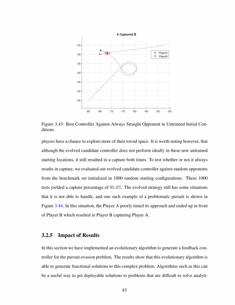
-85 -80 -75 -70 -65 -60 -55 -50
-55
-50
-45
-40
-35
-30
-25
A Captured B
PlayerAPlayerB
Figure 3.43: Best Controller Against Always Straight Opponent in Untrained Initial Con-ditions
players have a chance to explore more of their toroid space. It is worth noting however, that
although the evolved candidate controller does not perform ideally in these new untrained
starting locations, it still resulted in a capture both times. To test whether or not it always
results in capture, we evaluated our evolved candidate controller against random opponents
from the benchmark set initialized in 1000 random starting configurations. These 1000
tests yielded a capture percentage of 95.3%. The evolved strategy still has some situations
that it is not able to handle, and one such example of a problematic pursuit is shown in
Figure 3.44. In this situation, the Player A poorly timed its approach and ended up in front
of Player B which resulted in Player B capturing Player A.
3.2.5 Impact of Results
In this section we have implemented an evolutionary algorithm to generate a feedback con-
troller for the pursuit-evasion problem. The results show that this evolutionary algorithm is
able to generate functional solutions to this complex problem. Algorithms such as this can
be a useful way to get deployable solutions to problems that are difficult to solve analyti-
83

-40 -30 -20 -10 0 10
-90
-85
-80
-75
-70
-65
-60
-55
-50
-45
-40
B Captured A
PlayerAPlayerB
Figure 3.44: Player A Gets Captured by Player B from Untrained Initial Conditions
cally. Future work will aim to develop more robust solutions by adding more diverse initial
conditions, and experimenting with different controller representations. Furthermore, we
will attempt to expanded upon the methods used here to investigate the co-evolution of both
pursuer and evader.
84

Conclusion and Future Work
4.1 Conclusion
In conclusion, we can see that if properly implemented, evolutionary algorithms can be
used to generate near optimal solutions to many different types of path planning problems.
From simple problems such as the open-loop turn circle intercept problem to more complex
problems such as closed-loop single pursuer single evader, the EA is able to develop a
solution that allows the agent to navigate to the desired goal in a near optimal way. By
using custom controller representations we were able to represent solutions in an easy to
read way while also making them simple to implement and evolve. By comparing the
evolved solutions to known optimal solutions, we were able to validate EA and show that
it is indeed converging on near optimal results. This validation helps build confidence in
the evolutionary methodology and can be used as justification to apply this method to more
complex problems in which the optimal solution is not known.
4.2 Future Work
Future work will aim to use the evolutionary framework presented in this thesis to develop
solutions to more complex problems that have yet to be analytically solved. This includes
scenarios such as multiple targets or scenarios in which there are multiple attackers that
85

must cooperate in order to reach their goal. Additionally, we hope to begin examining co-
evolutionary scenarios in which both the attacker and the target can evolve their solutions
throughout the generations. We also aim to further refine and experiment with our custom
controller representations.
86

Bibliography
[1] L. E. Dubins, “On curves of minimal length with a constraint on average curvature,
and with prescribed initial and terminal positions and tangents,” American Journal of
Mathematics, vol. 79, no. 3, pp. 497–516, Jul 1957.
[2] D. W. Casbeer, E. Garcia, Z. E. Fuchs, and M. Pachter, “Cooperative target defense
differential game with a constrained-maneuverable defender,” in 2015 54th IEEE
Conference on Decision and Control (CDC), Dec 2015, pp. 1713–1718.
[3] Z. E. Fuchs and P. P. Khargonekar, “Encouraging attacker retreat through defender
cooperation,” in 50th Conference on Decision and Control and European Control
Conference (CDC-ECC), Dec 2011, pp. 235–242.
[4] ——, “Generalized engage or retreat differential game with escort regions,” IEEE
Transactions on Automatic Control, vol. 62, no. 2, pp. 668–681, Feb 2017.
[5] S. Oussedik, D. Delahaye, and M. Schoenauer, “Dynamic air traffic planning by
generic algorithms,” Proceedings of the Congress on Evolutionary Computation,
vol. 2, pp. 1110–1118, 1999.
[6] M. Duarte, J. Gomes, S. Oliveira, , and A. Christensen, “Evolution of repertoire-based
control for robots with comple locomotor systems,” Transactions on Evolutionary
Computation, accepted for publication in future issue of this journal.
87

[7] C.Hocaoglu and A.C.Sanderson, “Planning multiple paths with evolutionary specia-
tion,” IEEE Transactions of Evolutionary Computation, vol. 5, no. 3, pp. 169–191,
June 2001.
[8] N. K. J. Kok, L. F. Gonzalez, “Fpga implementation of an evolutionary algorithm
for autonomous unmanned aerial vehicle on-board path planning,” Transactions on
Evolutionary Computation, vol. 17, pp. 272–281, April 2013.
[9] S. Mohseni, V. Duchaine, and T. Wong, “A comparative study of the optimal con-
trol design using evolutionary algorithms: Application on a close-loop system,” in
Intelligent Systems Conference, Sept 2017.
[10] K. Stanley and R. Miikkulainen, “Evolving neural networks through augmenting
topologies,” Evolutionnary Computation, vol. 10, no. 2, pp. 99–172, 2002.
[11] L. P. F. Gruau, D. Whitley, “A comparison between cellular encoding and direct en-
coding for genetic neural networks,” in Proc. 1st Annual Confernce on Genetic Pro-
gramming, 1996, pp. 81–89.
[12] C. Igel, “Neuroevolution for reinforcement learning using evolution strategies,” in
IEEE Congress on Evolutionrary Computation, 2003.
[13] R. M. N. Kohl, “Evolving neural networks for fractured domains,” in Proceedings on
Genetic and Evolutionary Computation, 2008.
[14] N. Kohl and R. Miikkulainen, “Evolving neural networks for strategic decision-
making problems,” in Neural Networks, Special issue on Goal-Directed Neural Sys-
tems, 2009.
[15] Multi-Command Handbook 11 F-16. United States Air Force, 1996.
[16] P.Androulakakis and Z.E.Fuchs, “Evolutionary design of engagement strategies for
turn-constrained agents,” in IEEE Congress on Evolutionary Computation, May 2017.
88
[17] Z. E. Fuchs, D. W. Casbeer, and E. Garcia, “Singular analysis of a multi-agent, turn-
constrained, defensive game,” in American Control Conference (ACC), 2016, July
2016, to appear May 2016.
[18] A. Merz, “The homicidal chauffeur,” AIAA Journal, vol. 12, no. 3, pp. 259–260, 1974.
[19] Z. E. Fuchs, P. P. Khargonekar, and J. Evers, “Cooperative defense within a single-
pursuer, two-evader pursuit evasion differential game,” in 49th Conference on Deci-
sion and Control, Dec. 2010, pp. 3091–3097.
[20] E. Konaka, “Design of discrete predictive controller using approximate nearest neigh-
bor method,” in Proceedings of IFAC 18th World Contress, vol. 44, no. 1, 2011, pp.
10 213 – 10 218.
[21] F. Lin, M. Fardad, and M. Jovanovic, “Optimal control of vehicular formations with
nearest neighbor interactions,” IEEE Transactions on Automatic Control, vol. 57,
no. 9, pp. 2203–2218, 2012.
89

90