A Survey on Localization in Wireless Sensor networks

Zheng Yang

Supervised By

Dr. Yunhao Liu

Abstract Recent technological advances have enabled the development of low-cost, low-power,

and multifunctional sensor devices. These nodes are autonomous devices with integrated sensing, processing, and communication capabilities. In general, wireless sensor networks intend to provide information on spatio-temporal characteristics of the observed physical world. Hence, it is necessary to associate sensed data with locations, making data geographically meaningful. A number of applications, such as object tracking, environment monitoring, inherently rely on location information. Besides, location information also supports fundamental network layer services, such as topology control, routing, clustering, and so on. Hence, Localization, a mechanism for autonomously discovering and establishing spatial relationships among sensor nodes, is of great importance in the development of wireless sensor networks. This survey reviews diverse physical measuring abilities of sensor nodes, discusses issues in localization algorithm design, presents the state-of-the-art localization techniques, and finally suggests future directions in localization studies. Many localization approaches are proposed based on diverse positioning principles, environmental constrains, accuracy requirements, etc., making them suitable/unsuitable for different applications. This survey in depth elaborates and compares existing approaches from two aspects: physical measurement and network-wide localization. The design tradeoffs of localization algorithms, as well as their advantages and disadvantages, are emphasized for comparison. Among these localization techniques, no specific algorithm is a clear favorite across the spectrum. In conclusion, localization is a new and exciting field, with new algorithms, hardware, and applications being developed at a feverish pace. A lot of work still needs to be done to realize practical applications for wireless sensor networks.

Contents 1. Introduction........................................................................................................................ 6 2. Physical measurements ...................................................................................................... 7

2.1. Distance measurement............................................................................................ 8 2.1.1. Radio signal strength based distance measurement .................................... 9 2.1.2. Time Difference of Arrival (TDoA).......................................................... 10

2.2. Angle measurement .............................................................................................. 12 2.2.1. Angle of Arrival (AoA)............................................................................. 12

2.3. Area measurement ................................................................................................ 13 2.3.1. Single reference area estimation ............................................................... 13 2.3.2. Multi-reference area estimation ................................................................ 14

2.4. Hop count measurements ..................................................................................... 15 2.5. Neighborhood measurement................................................................................. 17

2.5.1. Single neighbor proximity ........................................................................ 17 2.5.2. K-neighbor proximity................................................................................ 18 2.5.3. ID-CODE .................................................................................................. 18

2.6. Comparative study................................................................................................ 19 3. Network-wide localization............................................................................................... 20

3.1. Issues in localization algorithm design................................................................. 20 3.1.1. Beacon nodes ............................................................................................ 20 3.1.2. Node density ............................................................................................. 21 3.1.3. System organization.................................................................................. 21

3.2. Centralized localization approaches ..................................................................... 22 3.2.1. Multi-dimensional scaling (MDS) ............................................................ 22 3.2.2. Semidefinite programming (SDP) ............................................................ 22

3.3. Distributed localization approaches ..................................................................... 23 3.3.1. Beacon based localization......................................................................... 23 3.3.2. Coordinate system stitching ...................................................................... 24

3.4. Comparative study................................................................................................ 26 4. Future directions .............................................................................................................. 26 5. Conclusion ....................................................................................................................... 27

List of figures: Figure 1: Telos hardware platform .................................................................................... 6 Figure 2: Physical measurements ...................................................................................... 7 Figure 3: Trilateration........................................................................................................ 8 Figure 4: Radio signal attenuation................................................................................... 10 Figure 5: TDoA hardware model..................................................................................... 10 Figure 6: TDoA computation model.................................................................................11 Figure 7: Area measurements .......................................................................................... 14 Figure 8: APIT................................................................................................................. 15 Figure 9: Hop count measurement .................................................................................. 16 Figure 10: Distance mismatch ......................................................................................... 16 Figure 11: k-neighbor proximity...................................................................................... 18 Figure 12: GPS ................................................................................................................ 20 Figure 13: SDP ................................................................................................................ 23 Figure 14: Beacon based localization.............................................................................. 24 Figure 15: Iterative localization....................................................................................... 24 Figure 16: Coordinate system stitching ........................................................................... 25

List of tables Table 1: Comparative study of physical measurements .................................................. 19 Table 2: Comparative study of localization algorithms................................................... 26

1. Introduction

Recent technological advances have enabled the development of low-cost, low-power, and multifunctional sensor devices. These nodes are autonomous devices with integrated sensing, processing, and communication capabilities. A sensor node is an electronic device that is capable of detecting environmental conditions such as temperature, sound, chemicals, or the presence of certain objects, as shown in Figure 1 [56]. The envisioned applications of these wireless sensor networks range widely: ecological habitat monitoring [40], structure health monitoring [75], environmental monitoring [71], industrial process control [41], and object tracking [32], among others.

Figure 1: Telos hardware platform

Wireless sensor networks [2, 31] are emerging and a lot of efforts are made in several aspects, including network topology control [45, 54, 59, 64, 69, 70, 76], localization [6, 17, 24, 26, 33, 37, 43, 49, 51, 62, 65], time synchronization [16, 22, 42, 66], embedded operating system [9, 14, 25, 27], routing [5, 20, 29, 80], in-network data aggregation [10, 19, 34, 39, 47, 67, 77, 78], reliable transmission and congestion control [15, 28, 61, 68], and sensor security and privacy [8, 12, 13, 18, 36, 55], etc.

Wireless sensor networks are fundamentally intended to provide information about the spatio-temporal characteristics of the observed physical world. Hence, it is necessary to associate sensed data with locations, making data geographically meaningful. A number of applications, such as object tracking, environment monitoring, inherently rely on location information. Besides, location information also supports fundamental network layer services, such as topology control, routing, and clustering. Hence, Localization, a mechanism for autonomously discovering and establishing spatial relationships among sensor nodes, is of great importance in the development of wireless sensor networks. In this survey, we review the existing localization approaches from two aspects: the physical measurement and the network-wide localization. Generally, nearly all localization algorithms consist of such two stages in a way that first perform physical measuring to gather data, and then do localization based on such data. Here physical measurement means a way

for obtaining physical geometric relations in local map, such as detecting neighbor nodes and ranging the inter-node distance or angle. Other than determining the location of a single unknown node given a number of nearby references, a broader problem is that of network localization, where a large number of unknown nodes have to be localized in a network with a few reference nodes. The design of network localization algorithms depend very much on the resource availability and the accuracy requirements. A number of localization approaches are proposed based on diverse positioning principles, environmental constrains, accuracy requirements, and so on, making them suitable/unsuitable for different applications. We elaborate and compare the advantages and disadvantages of existing localization approaches. Generally, localization algorithms depend heavily on a variety of factors such as application needs and available physical measurements. No specific algorithm is a clear favorite across the spectrum. The rest of this survey is organized as follows. Section 2 elaborates the physical measurements by using diverse measuring hardware. The analysis of localization algorithms, as well as the design issues, is given in section 3. Section 4 discusses some hot topics and the future directions of this field. Finally, section 5 concludes this survey.

2. Physical measurements

It is inherently infeasible to do localization without the knowledge of physical world. Thus in all existing localization approaches, sensor nodes are required to measure physical geometric elements to some extent. According to the abilities of diverse localization hardware, we classify the physical measurements (and the corresponding measuring techniques into several types (from fine-grained to coarse-grained): position information, distance, angle, area, hop count, and neighborhood, as shown in Figure 2.

Figure 2: Physical measurements

Among them, the most powerful physical measurement is directly obtaining the position without any further computation. GPS is such a kind of infrastructure. However, the pure GPS solution is viable only if all nodes in the network can be provided with a potentially expensive GPS receiver and if the deployed area provides good satellite coverage, which makes it infeasible for many applications. Different form the directly location information, the remaining five physical measurements are used in the scenarios of positioning an unknown node by given a number of reference nodes. Here the term “unknown” means being not aware of location; while the term

“reference” means the localized nodes used to locate other unknown ones. The former two, distance and angle measurements, are based on some ranging techniques; while the latter two, hop count and neighborhood, are basically based on radio connectivity. The middle one, area measurement, relies on either ranging or connectivity depending on how the area constrains being formed.

2.1. Distance measurement

The distances from an unknown node to several reference positions help to constrain the presence of this node, which is the basic idea of the so called multilateration technique. To accurately and uniquely determine the relative location of a point on a 2D plane, generally at least 3 reference points are needed. Figure 3 shows an example of trilateration, a special form of multilateration which utilizes exact three references. The object to be localized (the soft dot) measures the distances from itself to three references (the solid dots). Obviously, this object should be located at the circle centered at each reference position. Thus, the intersection of three circles is treated as the estimated location of this object. The result of trilateration is a unique position as long as three references are non-linear.

Figure 3: Trilateration

Multilateration is a simple technique, but the specific mathematics of its implementation vary widely, as do its application in sensor networks. Suppose the location of the unknown node is (x0, y0) and it is able to obtain the distance estimates d’i to the ith reference node locating in (xi, yi), 1 ≤ i ≤ n. Let di be the actual Euclidean distance to the ith reference node, i.e.:

2 20 0( ) ( )i i id x x y y= − + − .

Thus the difference between the measured and actual distance can be represented as ρi = d’i - di. Several methods are designed to deal with the ranging noise. The least squares

minimization is one of them to determine the value of (x0, y0) that minimizes 2

1

n

iiρ

=∑ . This

problem can be solved by a numerical solution to an over-determined linear system [62].

We rewrite the distance constrains as follows: Ax = B, where A is an (n-1)×2 matrix, such that the ith row of A is [2(xi - xn) 2(yi - yn)], x is the column vector representing the coordinates of the unknown location [x0 y0]T, and B is the (n-1) element column vector whose ith term is the expression (xi

2 + yi2 - xn

2 - yn2 - di

2 + dn2). In practice, we cannot determine B, since the

actual distances are unknown to us. So computation is performed on B’, which is the same as B with d’i substituting for di. Now the least square solution is an estimate for x’ that minimizes ||Ax’ – B’||2, which is provided by x’ = (ATA)-1ATB’. As mentioned above, localization can be realized by multilateration if distance measurements are available. The only thing omitted is how to measure distance in real physical world. Many efforts are made in this topic and a number of ranging techniques are developed in recent years. Among of them, the Radio signal strength based and time based ranging are two of the most widely used approaches in today’s application.

2.1.1. Radio signal strength based distance measurement

RSS based ranging techniques rely on the fact that the strength of radio signal diminishes during propagation. As a result, the understanding of radio attenuation helps to map signal strength to distance. In other words, a node listening to a radio transmission is able to use the strength of the received signal to calculate its distance from the transmitter. In theory, radio signal strengths diminish with distance according to a power law. One model that is used for wireless radio propagation is the following [63]:

00

( ) ( ) 10log dP d P d Xd ση

⎛ ⎞= − +⎜ ⎟

⎝ ⎠

where P(d) is the received power at distance d and p(d0) is the received power at some reference distance d0, η the path-loss exponent, and Xσ a log-normal random variable with variance σ2 that accounts for fading effects. So, if the path-loss exponent for a given environment is known, the received signal strength can be used to estimate the distance.

In practice, however, RSS-based ranging measurements contain noise on the order of several meters [4], especially in rigorous environments [79]. The ranging noise occurs because radio propagation tends to be highly dynamic as shown in Figure 4.

Figure 4 is obtained by deploying a testbed system in HKUST campus (outdoor environment). The hardware layer of the testbed is constructed on the Telos motes with Atmel128 processor and CC2420 transceiver. We fit each node with a shelf, which supports the sensor node 150cm above ground. The transmitting power of sensor nodes is set to 1mW and the transmitting range could reach as far as 50m with more than -90dbm receiving signal strength. We construct a distance estimator according to the signal propagation model: the log-normal shadowing model [38, 63].

According to Figure 4, there is an overall trend that the RSS value decreases with increasing distance. However, this trend is not monotonic and there are remarkable fluctuations. This irregularity can be attributed to a number of reasons. For instance, radio propagates differently over asphalt than over grass. In addition, physical obstacles such as walls, furniture, and the like, reflect and absorb radio waves.

0 5 10 15 20 25 30 35 40-100

-90

-80

-70

-60

-50

-40

-30

-20

Distance (m)

RS

SI (d

B)

Figure 4: Radio signal attenuation

On the whole, RSS based ranging is a relatively "cheap" solution without any extra devices, as all sensor nodes are likely to have radios. The performance, however, is not as good as other ranging techniques due to the multipath propagation of radio signals. It is believed that more careful physical analysis of radio propagation may allow better use of RSSI data, thus improving the localization accuracy. Nevertheless, the breakthrough technology is not there today.

2.1.2. Time Difference of Arrival (TDoA)

As we have seen, RSS based technique significantly suffers from the irregularity of RF signal propagation. A more promising technique is the combined use of ultrasound/acoustic and radio signals to estimates distances by determining the Time difference of arrival (TDoA) of these signals [57, 62, 73]. This technique is a commonly used hardware ranging mechanism, in which each node is equipped with a speaker and a microphone, shown in Figure 5. Some systems use ultrasound while others use audible frequencies. The general mathematical technique, however, is independent of particular hardware.

Figure 5: TDoA hardware model

The idea of TDoA ranging is conceptually quite simple, illustrated in Figure 6. The transmitter first sends a radio signal. It waits some fixed internal of time, tdelay (which might be zero), and then produces a fixed pattern of "chirps" on its speaker. When receivers hear the radio signal, they note the current time, tradio, and then turn on their microphones. When their microphones detect the chirp patter, they again note the current time, tsound. Once they have tradio, tsound, and tdelay, the receivers can compute the distance d between themselves and the transmitter using

radio soundsound radio delay

radio sound

( )v vd t t tv v

⋅= ⋅ − −

−,

where vradio and vsound denote the speed of radio and sound waves respectively. Since radio waves travel substantially faster than sound in air, the distance is then simply estimated as d = vsound· (tsound - tradio - tdelay). If the design is transmitting radio and acoustic signals simultaneously, i.e., tdelay = 0, the estimation can be further simplified as vsound·(tradio - tsound).

Figure 6: TDoA computation model

TDoA methods are impressively accurate under line-of-sight conditions. For instance, it is claimed in [62] that distance can be estimated to within a few centimeters for node separations under 3 meters. The cricket ultrasound system [57] can obtain close to centimeter accuracy without calibration over ranges of up to 10 meters in indoor environments. Though accurate it is, TDoA systems are constrained by the line-of-sight condition, which can be difficult to meet in some environments. In addition, TDoA systems perform better when they are calibrated properly, since speakers and microphones never have identical transmission and reception characteristics. Furthermore, the speed of sound in air varies with air temperature and humidity, which introduce inaccuracy into distance estimation. Acoustic signals also show multi-path propagation effects that may impact the accuracy of signal detection. These can be mitigated to a large extent using simple spread-spectrum techniques, such as those described in [23]. The basic idea is to send a pseudo-random noise sequence as the acoustic signal and use a matched filter for detection, instead of using a simple chirp and threshold detection. Recently, researchers [53] observed that two intrinsic uncertainties in TDoA measuring process that can contribute to the ranging inaccuracy: the possible misalignment between the sender timestamp and the actual signal emission, and the possible delay of a sound signal arrival being recognized at receiver. In general, many factors can cause these uncertainties in

a real system, such as the lack of real-time control, software delay, interrupt handling delay, system loads, etc. They also pointed out that that these two delays, if not controlled, can easily add up to several milliseconds on average, which translates to several feet of ranging error. By designing BeepBeep [53], a high-accuracy acoustic-based ranging system, the localization accuracy can achieve one or two centimeters accuracy within a range of more than ten meters, which is so far the best result of ranging on off-the-shelf cell phones. In the end, many localization algorithms use time difference of arrival ranging simply because it is dramatically more accurate than radio-only methods. The tradeoff is that sensor nodes must be equipped with acoustic transceivers in addition to radio transceivers. The actual reason why TDoA is more effective in practice than RSS is due to the difference between using signal travel time and signal magnitude, where the former is vulnerable only to occlusion while the latter is vulnerable to both occlusion and multipath [3].

2.2. Angle measurement

Another possibility for localization is the use of angular estimates instead of distance estimates. In trigonometry and geometry, triangulation is the process of finding coordinates and distance to a point by calculating the length of one side of a triangle, given measurements of angles and sides of the triangle formed by that point and two other known reference points, using the law of sines. Unlike trilateration, which uses distance measurements to calculate the object's location, triangulation uses the measured angle information between the object and each reference point, together with at least one known distance. Triangulation is once used to find the coordinates and sometimes distance from the shore to the ship.

2.2.1. Angle of Arrival (AoA)

The Angle of Arrival (AoA) data are typically gathered using radio or microphone arrays, which allow a receiver to determine the direction of a transmitter. It is also possible to gather AoA data from optical communication methods. In the methods, several (3-4) spatially separated microphones hear a single transmitted signal. By analyzing the phase or time difference between the signal's arrival different microphones, it is possible to discover the AoA of the signal. These methods can obtain accuracy to with a few degrees [58]. A very simple localization technique, involving three rotating reference beacons at the boundary of a sensor network providing localization for all interior nodes, is described in [46]. A more detailed description of AoA-Based triangulation techniques is provided in [50]. Unfortunately, AoA hardware tends to be bulkier and more expensive than TDoA ranging hardware, since each node must have one speaker and several microphones. Furthermore, the need for spatial separation between microphones is difficult to accommodate in small size sensor nodes. Generally, AoA techniques provide more accurate localization result than RSS based ones, however, compared with TDoA ranging, no notably improvement is gained.

Considering the cost of AoA ranging hardware, few localization algorithms absolutely require AoA information in practice, though several are capable of using it when it is present.

2.3. Area measurement

If the bounds on radio or other signal coverage for a given node can be described by a geometric shape, this can be used to provide location estimates by determining which geometric areas that a node is constrained to be in. The basic idea of area estimation is to compute the intersections among all overlapping coverage regions and choose the centroid as the location estimate. Along with the increasing number of constraining areas, more localization accuracy can be achieved. According to how area is estimated, we divide the existing work into two kinds: single reference area estimation and multi-reference area estimation.

2.3.1. Single reference area estimation

Single reference estimation means that areas are obtained in a pairwise manner, i.e., the information of a geometric area comes from only one reference at each stage. For instance, the region of radio coverage may be upper-bounded by a circle of radius Rmax. In other words, if node B hears node A, it knows that it must be no more than a distance Rmax from A. Now, if an unknown node hears from several reference nodes, it can determine that it must lie in the geometric region described by the intersection of circles of radius Rmax centered on these nodes, illustrated in Figure 7(a). This can be extended to other scenarios. For instance when both lower bound Rmin and upper bound Rmax can be determined, based on the received signal strength, the shape of a single node's coverage is an annulus, illustrated in Figure 7(c); when an angular sector (θmin, θmax) and a maximum range Rmax can be determined, the shape for a single node's coverage would be a cone with given angle and radius, illustrated in Figure 7(d).

Localization techniques using geometric regions were first described by [11]. One of the nice features of these techniques is that not only can the unknown nodes use the centroid of the overlapping region as a specific location estimate if necessary, but they can also determine a bound on the location error using the size of this region. When the upper bounds on these regions are tight, the accuracy of this geometric approach can be further enhanced by incorporating "negative information" about which reference nodes are not within range [21]. Although arbitrary shapes can be potentially computed in this manner, a computational simplification that can be used to determine this bounded region is to use rectangular bounding boxes as location estimates. The bounding-box algorithm [62] is a computationally simple method of localization nodes given their ranges to several references. Essentially, each node assumes that it lies within the intersection of its reference's bounding boxes.

The bounding box for a reference is centered at the reference position (xi, yi), and has height and width 2 × di. The intersection of the bounding boxes can be computed without use of floating point operations: [max(xi - di), max(yi - di)] × [min(xi + di), min(yi + di)]. The position of a node is then the center of this final bounding box, as shown in Figure 7(b).

(a) (b)

(c) (d) Figure 7: Area measurements

Whitehouse [72] analyzes a distributed version of bounding box algorithm, showing that unfortunately this version is highly susceptible to noisy range estimates, especially small estimates that tend to propagate. The accuracy of the bounding-box approach is best when the nodes' actual position is closer to the center of their references. Bounding box works best when sensor nodes have extreme computational limitations, since other algorithms may simply be infeasible. Otherwise, more mathematically rigorous approaches such as multilateration may be more appropriate.

2.3.2. Multi-reference area estimation

A related approach to localization using area estimation is the approximate point in triangle (APIT) technique [26]. Its novelty lies in how the regions are defined as triangles between different sets of three reference nodes, rather than the coverage of a single node. Basically, APIT consists of two key processes: triangle intersection and point in triangle (PIT) test. In APIT, nodes are assumed to be able to hear a fairly large number of beacons. A node forms some number of "reference triangles", where a reference triangle is the triangle formed by three arbitrary references. The node then decides whether it is inside or outside a given triangle by PIT test. Once this process is complete, the node simply finds the intersection of the reference triangles that contains it and chooses the centroid as its position estimate. This is illustrated in Figure 8. In this process, APIT does not assume that nodes can range to these beacons.

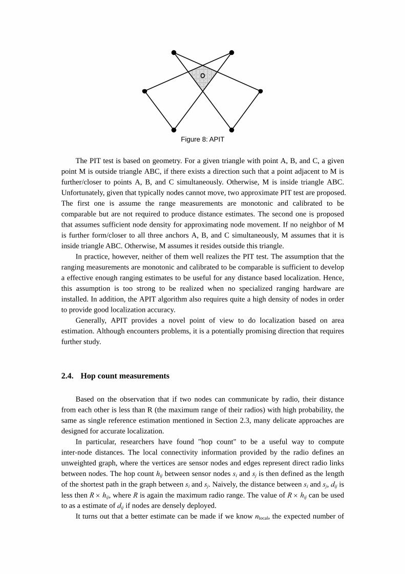
Figure 8: APIT

The PIT test is based on geometry. For a given triangle with point A, B, and C, a given point M is outside triangle ABC, if there exists a direction such that a point adjacent to M is further/closer to points A, B, and C simultaneously. Otherwise, M is inside triangle ABC. Unfortunately, given that typically nodes cannot move, two approximate PIT test are proposed. The first one is assume the range measurements are monotonic and calibrated to be comparable but are not required to produce distance estimates. The second one is proposed that assumes sufficient node density for approximating node movement. If no neighbor of M is further form/closer to all three anchors A, B, and C simultaneously, M assumes that it is inside triangle ABC. Otherwise, M assumes it resides outside this triangle. In practice, however, neither of them well realizes the PIT test. The assumption that the ranging measurements are monotonic and calibrated to be comparable is sufficient to develop a effective enough ranging estimates to be useful for any distance based localization. Hence, this assumption is too strong to be realized when no specialized ranging hardware are installed. In addition, the APIT algorithm also requires quite a high density of nodes in order to provide good localization accuracy. Generally, APIT provides a novel point of view to do localization based on area estimation. Although encounters problems, it is a potentially promising direction that requires further study.

2.4. Hop count measurements

Based on the observation that if two nodes can communicate by radio, their distance from each other is less than R (the maximum range of their radios) with high probability, the same as single reference estimation mentioned in Section 2.3, many delicate approaches are designed for accurate localization. In particular, researchers have found "hop count" to be a useful way to compute inter-node distances. The local connectivity information provided by the radio defines an unweighted graph, where the vertices are sensor nodes and edges represent direct radio links between nodes. The hop count hij between sensor nodes si and sj is then defined as the length of the shortest path in the graph between si and sj. Naively, the distance between si and sj, dij is less then R × hij, where R is again the maximum radio range. The value of R × hij can be used to as a estimate of dij if nodes are densely deployed. It turns out that a better estimate can be made if we know nlocal, the expected number of

neighbors per node. Then, as shown by Kleinrock and Silvester [30], it is possible to compute a better formula for the distance covered by one radio hop:

21 ( / )arccos 1

1(1 )local localn n t t t

hopd R e e dtπ− − − −

−= + − ∫ .

Then dij ≈ hij × dhop. Experimentally [44], equation above has been shown to be quite accurate when nlocal grows above 5. However, when nlocal > 15, dhop approaches R, so the equation of dhop becomes less useful. Nagpal et al. [44] demonstrate by algorithm that even better hop-count distance estimates can be computed by averaging distances with neighbors. This benefit does not begin to appear until nlocal ≥ 15; however, it can reduce hop-count error down to as little as 0.2R.

Figure 9: Hop count measurement

Another method to estimate per-hop distance is to employ a number of reference nodes, illustrated in Figure 9. As the locations of reference nodes are known, the distance between them can be readily computed. Hence, if the hop count hij between two references (si and sj ) and the distance dij are available, the per-hop distance can be estimated as dhop = dij / hij.

(a) (b)

Figure 10: Distance mismatch

Due to the hardware limitations and energy constraints of sensor devices, hop count

based localization approaches are cost-effective alternatives to ranging based approaches. Since there is no way of measuring physical distances among nodes, existing hop count based approaches largely depend on connectivity measurements with a high density of seeds.

Most existing approaches, however, would fail in anisotropic sensor networks, where holes exist among sensor nodes, as shown in Figure 10. In anisotropic networks [35], the Euclidean distances between a pair of nodes may not correlate closely with the hop counts between them because the path between them may have to curve around intermediate holes, resulting poor localization accuracy. Indeed, anisotropic networks are more likely to exist in practice for several reasons. First, in many real applications, sensor nodes/seeds can rarely be uniformly deployed over the field due to the geographical obstacles. Second, even if we assume that the initial sensor network is isotropic, unbalanced power consumption among nodes will likely create holes in the network. Recently, a distributed method [24] has been proposed to detect hole boundary by using only the connectivity information. Based on that work, REP [33] is proposed to deal with the “distance mismatch” problem in anisotropic networks.

2.5. Neighborhood measurement

Wireless sensor networks are designed to perform data collecting and communicating. Thus, in wireless sensor networks, the radio connectivity measurement can be considered economic due to the absence of any extra hardware. We classify the existing localization approaches based on neighborhood information into several types according to how and to what extent they use the neighborhood information. From simple to complicated, they are single neighbor proximity, k-neighbor proximity, ID-CODE.

2.5.1. Single neighbor proximity

Perhaps the most basic location technique is that of one neighbor proximity - involving a simple decision of whether two nodes are within reception range of each other. A set of reference nodes is placed in the environment with some non-overlapping (or nearly non-overlapping) subregions. Either the reference nodes periodically emit beacons, or the unknown node transmits a beacon when it needs to be localized. If reference nodes emit beacons, there include their location IDs. The unknown node then uses the received location information as its own location, providing a course-grained localization. A little more complicated method is to determine which reference nodes the unknown node is closest to, in case a number of reference nodes are within the communication ranging. Alternatively, if the unknown node emits a beacon, the reference node that hears the beacon uses its own location to determine the location of the unknown node. The major advantage of this single neighbor proximity approach is the simplicity of computation, which is desirable to resource-constrained sensor nodes.

2.5.2. K-neighbor proximity

The neighborhood information can be used to greater advantage when the density of reference nodes is sufficiently high that there are several reference nodes within the range of the unknown node. Let there be k reference nodes detected within the proximity of the unknown node, with the location of the ith reference denoted by (xi, yi). Then, in this technique, the location of the unknown node (x0, y0) is determined as

01

01

1

1

k

ii

k

ii

x xk

y yk

=

=

= ⋅

= ⋅

∑

∑

This is actually a k-nearest-neighbor approximation in which all reference nodes have equal weights, as shown in Figure 11. The centroid of the polygon (the red dot), constructed by reference nodes, is the estimated position of the unknown node.

Figure 11: k-neighbor proximity This simple centroid technique has been investigated using a model with each node having a simple circular range R in an infinite square mesh of reference nodes spaced a distance d apart [6]. It is shown through simulation that, as the overlap ratio R/d is increased from 1 to 4, the average error in localization is reduced from 0.5d to 0.25d. The k-neighbor proximity approach inherits the merit of computational simplicity from one neighbor proximity approach; while at the same time, provides more accurate localization result than single neighbor proximity statistically. However, using centroid as estimate still may cause relatively large error, which is significantly degrades the quality of localization in case of iterative approaches are used due to the error propagation.

2.5.3. ID-CODE

There is another interesting technique that utilizes overlapping coverage regions to provide localization [60]. In this technique, the sensor deployment is planned in such a way as to ensure that each location is covered by a unique set of sensors. Hence, the uniqueness can

be used for localization. The key problem in this technique is how to distribute the identifying code to each region. The algorithm ID-CODE [60] is proposed to construct such an identifying code based on neighborhood information. Once this is done, each location region will be covered by a unique set of reference nodes. However, the planned deployment is usually not suitable for many applications. In General, we assume wireless sensor networks are consists of a large number of sensor nodes, making the planned deployment, if not infeasible, time-consuming in practice. Another drawback of ID-CODE is the identifying code construction is computational expensive. In theory, obtaining a minimal identifying code is known to be NP-Complete, although the algorithm ID-CODE is a polynomial greedy heuristic that provides good solutions in practice.

2.6. Comparative study

In this section, a comparative study is given for the existing physical measurement approaches. Table 1 provides an overview of these approaches in terms of accuracy, hardware cost, and environment requirements. All approaches have their own merits and drawbacks, making them suitable for different applications.

Table 1: Comparative study of physical measurements

Physical Measurements AccuracyHardware

Cost Computation Cost

RSS Median Low Low Distance

TDoA High High Low Angle AoA High High Low

Single reference

Median* Median* Median Area

Multi-reference Median* Median* High

Hop count Per-hop distance

Median Low Median

Single neighbor Low Low Low Multi-neighbor Low Low Low Neighborhood

ID-CODE Low Low High *: depends on the diverse geometric constrains

3. Network-wide localization

3.1. Issues in localization algorithm design

3.1.1. Beacon nodes

Beacon nodes (also frequently called seeds or anchor nodes) are a necessary prerequisite to localizing a network in a global coordinate system. Beacon nodes are simply ordinary sensor nodes that known their global coordinates a priori. This knowledge could be hard-coded, or acquired through some additional hardware like a GPS receiver, as shown in Figure 12 [1]. At a minimum, three noncollinear beacon nodes are required to define a global coordinate system in two dimensions. The advantage of using beacons is obvious: the presence of several pre-localized nodes can greatly simplify the task of assigning coordinates to ordinary nodes.

Figure 12: GPS

It is of great importance to employ beacon nodes in localization, which is represented in two aspects: beacon configuration and how to use beacon information. Beacon placement, as a part of beacon configuration, can often have a significant impact on localization. Many groups have found that localization accuracy improves if beacons are placed in a convex hull around the network. Locating additional beacons in the center of the network is also helpful. In any event, there is considerable evidence that real improvements in localization can be obtained by planning beacon layout in the network. The number of beacon nodes in a network is another problem to which we need to pay much attention when design localization algorithms. Basically, we cannot have all sensor nodes being beacon nodes for many reasons. For instance, GPS receivers are expensive. They also cannot typically be used indoors, and can also be confused by tall buildings or other environmental obstacles. GPS receivers also consume significant battery power, which can be a problem for power-constrained sensor nodes. The alternative of GPS is preprogramming nodes with their locations, which can be impractical considering the large number of sensor nodes in a network. It may be even impossible in case of deploying nodes by aircrafts.

Basically there are two types of beacon nodes using: directly and indirectly. The former one means, when locating, unknown nodes find information directly from beacon nodes, no matter how far they are from beacon nodes. While the latter one indicates a group of algorithms in which unknown nodes obtain information only from their neighbors and become reference nodes in the following localization process after they have been located. The latter ones actually work in a so called iterative manner. In short, beacons are necessary for localization, but their use does not come without cost.

3.1.2. Node density

Many localization algorithms are sensitive to node density. For instance, hop-count-based schemes generally require high node density so that the hop count approximation for distance is accurate. Similarly, algorithms that depend on beacon nodes fail when the beacon density is not high enough in a particular region. Thus when designing or analyzing an algorithm, it is important to notice the algorithm's implicit density assumptions, since high node density can sometimes be expensive if not totally infeasible.

3.1.3. System organization

This subsection defines taxonomy for localization algorithm based on their computational organization. Centralized algorithms are deigned to run on a central machine with plenty of computational power. Sensor nodes gather environmental data and pass them back to a base station for analysis, after which the computed positions are transported back into the network. Because of the localization computation running on the base station, centralized algorithms solve the problem of nodes' computational limitations. This benefit, however, comes from accepting the communication cost of moving data back to the base station. Unfortunately, communication generally causes more energy consumptions than computation in existing sensor hardware platforms. In contrast, distributed algorithms are designed to run in the network, using massive parallelism and inter-node communication to compensate for the lack of centralized computing power and at the same time to reduce the expensive node-to-sink communication. Often distributed algorithm use a subset of the data to solve for each position independently, yielding an approximation of a corresponding centralized algorithm where all the data are considered and used to solve for all the positions simultaneously. There are two important approaches to distributed localization. The first group, beacon-based distributed algorithms, typically starts with some group of beacons. Nodes in the network obtain a distance measurement to a few beacons, and then use these measurements to determine their own location. In some algorithms, these newly localized nodes, become beacons to help other nodes localization, which is often called iterative localization. The second group approaches localization performs in a bottom-up manner. They work

in a bottom-up manner, in which localization is originated in a local group of sensors in relative coordinates. After gradually merging such local maps, it finally achieves entire network localization in global coordinates.

3.2. Centralized localization approaches

3.2.1. Multi-dimensional scaling (MDS)

Multi-dimensional scaling (MDS) is a centralized algorithm due to Shang [65]. MDS was originally developed for use in mathematical psychology. The intuition behind MDS is simple. Suppose there are n points, suspended in a volume. We do not know the positions of the points, but we do know the distance between each pair of points. MDS is an O(n3) algorithm that uses the law of cosines and linear algebra to reconstruct the relative positions of the points based on the pair wise distances. The algorithm has three stages, which are as follows: 1. Generate an n × n matrix M, whose (i, j) entry contains the estimated distance between nodes i and j. (simply run Floyd's all-pairs shortest-path algorithm). 2. Apply classical metric-MDS on M to determine a map that gives the locations of all nodes in relative coordinates. 3. Transform the solution into global coordinates based on some number of fixed anchor nodes. MDS performs well on RSSI data along, getting performance on the order of half the radio range when the neighborhood size nlocal is higher than 12 [3]. As expected, MDS-MAP estimates improve as ranging improves. The main problem with MDS, however, is its poor asymptotic performance, which is O(n3) on account of stages 1 and 2.

3.2.2. Semidefinite programming (SDP)

The semidefinite programming (SDP) approach to localization was pioneered by Doherty [11]. In this algorithm, geometric constraints between nodes, illustrated in Figure 13, are represented as linear matrix inequalities (LMIs). Once all the constraints in the network are expressed in this form, the LMIs can be combined to form a single semidefinite program. This is solved to produce a bounding region for each node, which Doherty simplifies to be a bound box. The advantage of SDP is its elegance by concise problem formulation, clear model representation, and elegant mathematic solution. Unfortunately, not all geometric constraints can be expressed as LMIs. In general, only constraints that form convex regions are amenable to representation as an LMI. Thus, AoA data can be represented as a triangle and hop count data can be represented as a circle, but precise range data cannot be conveniently represented, since rings cannot be expressed as convex constrains. This inability to accommodate precise range data may prove to be a significant drawback.

Figure 13: SDP

Solving the linear or semidefinite program must be done centrally. The relevant operation is O(k2) for angle of arrival data, and O(k3) when radial (e.g., hop count) data is included, where k is the number of convex constraints needed to describe the network. Thus, running time of SDP is not acceptable by some applications. Generally, SDP's efficiency problem is likely to preclude itself in practice.

3.3. Distributed localization approaches

3.3.1. Beacon based localization

Beacon based localization approaches utilize estimates of distances to reference nodes that may be several hops away [49, 51]. These distances are propagated from reference nodes to unknown nodes using a basic distance-vector technique. Such a mechanism can be seen as a top-down manner due to the progressive propagation of location information through entire networks. There are three types of this approach: 1. DV-hop: In this approach, each unknown node determines its distance from various reference nodes by multiplying the least number of hops to the reference nodes with an estimated average distance per hop. The average distance per hop depends upon the network density, and is assumed to be known. 2. DV distance: if inter-node distance estimates are directly available for each link in the graph, then the distance-vector algorithm is used to determine the distance corresponding to the shortest distance path between the unknown nodes and reference nodes, illustrated in Figure 14(a). 3. Euclidean propagation: Geometric relations can be used in addition to distance estimates to determine more accurate estimates to reference nodes. For instance consider a quadrilateral ABCR, illustrated in Figure 14(b), where A and R are at opposite ends; if node A knows the distances AB, AC, BC and nodes B and C have estimates of their distance to the reference R, then A can be use the geometric relations inherent in this quadrilateral to calculate an estimated distance to R.

(a) (b) Figure 14: Beacon based localization

Once distance estimates are available from each unknown node to different reference nodes throughout the network, a triangulation technique can be employed to determine their locations. Through simulations, it has been seen that location errors for most nodes can be kept within a typical single-hop distance [49]. One variant of this approach is to indirectly use of beacon nodes. Initially an unknown node, if possible, is located based on its neighbors by multilateration or other positioning techniques. After being aware of its location, it becomes a reference node to localize other unknown nodes in the following localization process. This step continues iteratively, gradually changing unknown nodes to known nodes. This process is illustrated in Figure 15.

Figure 15: Iterative localization

The advantage of this approach is that it only involves local information (information within neighborhood) when doing localization, resulting in high efficiency in terms of communication. However, the use of localized unknown nodes as reference nodes inherently introduces substantial cumulative error in the network localization. Some works [52, 74] concern the characteristics of error propagation in such multihop localization approaches and make efforts to limit such phenomena.

3.3.2. Coordinate system stitching

Coordinate system stitching is a different way of approaching the same problem. It has received a great deal of recent work [7, 43, 49]. It works as a bottom-up manner, in which

localization is originated in a local group of sensors in relative coordinates. After gradually merge such local maps, it finally achieve entire network localization in global coordinates, illustrated in Figure 16. Coordinate system stitching works according to the following algorithm: 1. Split the network into small overlapping subregions. Very often each subregion is simply a single node and its one-hop neighbors. 2. For each subregion, compute a "local map", which is essentially an embedding of the nodes in the subregion into a relative coordinate system. 3. Finally, merge the subregions using a coordinate system registration procedure. Coordinate system registration finds a rigid transformation that maps points in one coordinate system to a different coordinate system. Thus, step 3 places all the subregions into a single global coordinate system. Many algorithms do this step suboptimally, since there is a closed-form, fast and least-square optimal method of registering coordinate system.

Figure 16: Coordinate system stitching

Moore et al. [43] outline an approach that they claim produces more robust local maps. Rather than use three arbitrary nodes to define a map, Moore et al. use "robust quadrilateral" (robust quads), where a robust quad is a fully connected set of four nodes, where each subtriangle is also "robust". A robust subtriangle must have the property that:

b × sin2(θ) > dmin, where b is the length of the shortest side, θ is the size of the smallest angle, and dmin is a predetermined constant based on average measurement error. The idea is that the points of a robust quad can be placed correctly with respect to each other (i.e., without "flips"). Moore et al. demonstrate that the probability of a robust quadrilateral experiencing internal flips given zero mean Gaussian measurement error can be bounded by setting dmin appropriately. In effect, dmin filters out quads that have too much positional ambiguity to be localized with confidence. The appropriate level of filtering is based on the amount of uncertainty σ2 in the distance measurements. Unfortunately, coordinate System Stitching suffer from error propagation caused by local map stitching. Moore et al. prove the probability of their algorithm constructing correct local

maps and prove error lower bound on the local map positions. Furthermore, these techniques have a tendency to orphan nodes, either because they could not be added to a local map or because their local map failed to overlap sufficiently with neighboring maps. Moore et al. argue that this is acceptable because the orphaned nodes are the nodes most likely to display high error. They point out that "for many applications, missing localization information for a known set of nodes is preferential to incorrect information for an unknown set". However, this answer may not be satisfactory for some applications, many of which cannot use unlocalized nodes for sensing, routing, target tracking, or other tasks. Nevertheless, coordinate system stitching techniques are quite compelling. They are inherently distributed, since subregion and local map formation can trivially occur in the network and stitching is easily formulated as a peer-to-peer algorithm. Furthermore, they enable the use of sophisticated local-map algorithm which is too computationally expensive to use at the global level. For example, map formation using robust quadrilaterals is O(n4), where n is the number of nodes in the subregion; however, in networks with fixed neighborhood size nlocal, map formation is O(1). Likewise, coordinate system stitching enables the realistic use of O(n3) multidimensional scaling in sensor networks.

3.4. Comparative study

In this section, a comparative study is given for the existing localization approaches. Table 2 provides an overview of these approaches in terms of accuracy, node density, beacon percentage, computation cost, communication cost, and error propagation. All approaches have their own merits and drawbacks, making them suitable for different applications.

Table 2: Comparative study of localization algorithms

Localization Algorithm Accuracy Node

Density Beacon

PercentageComputa-tion Cost

Communi- cation Cost

Error Propagation

MDS High Low Low High High Low Centralized

SDP High Low Low High High Low Beacon based

Low High High Low Low High* Distributed

Coordinate stitching

Low High Low Median Median High

*: in case of iterative localization

4. Future directions

The sensor network field and localization in particular are in their infancy. Much work remains in order to address the varied localization requirements of sensor network services and applications. Many future directions stand out as important areas to pursue in order to

meet both current and future needs. In this section, two research topics will be emphasized, which we think may highly improve the existing localization techniques.

RSS based distance measurement generally suffers from large ranging noises, resulting in poor localization accuracy. For example, raw measurements of radio signal strength vary wildly from node to node, while most algorithms expect measurements to be at minimum monotonic and comparable. This fact causes several works that use more complicated solution to map the RSS value to distance. The RADAR [4] uses a pre-determined "map" of signal coverage in different locations of the environment. When doing localization, it uses this map to determine where a particular node is located by performing pattern matching on its measurements. This technique has some advantages; in particular as a pure RSS based technique, it has the potential to perform better than distance estimation. However, the key drawback of the technique is that it is very location specific and requires intensive data collection prior to operation. The LANDMARC [48] positioning system also use a "map" to record the relationship between RSS values and locations. Different from RADAR, the "map" is not required to be obtained in advance. By utilizing a number of "reference tags" deployed in known positions (for example, grid), LANDMARC match the RSS measurements of unknown nodes to the same measurements of reference tags, and find the nearest neighbor tags. From today’s techniques, it is very difficult to build the accurate propagation model of radio waves because many environmental factors influence the propagation process. Hence, many researchers begin to concern more complicated data analysis approaches for high quality localization.

Being quite popular because of the ease of implementation, multilateration based approaches are facing many challenges. First and foremost, although several ranging techniques are developed, including RSS and TDoA, error is inevitable in both of them. Thus the localization, especially in tough environments, turns out to be a failure because the noisy distance estimation largely degrades the quality of multilateration in the following four aspects: uncertainty, non-consistency, ambiguity, and error propagation. An increasing number of researchers begin to realize the importance of accurate localization under noisy ranging measurement. Error management [37] has been introduced for iterative localization to prevent error propagation, by analyzing the numerical features of multilateration. Alternative solutions are proposed from the view of geometric relations of reference nodes. According to Moore et al. [43], extra geometric constrains are added in the localization process to prevent the low quality multilateration.

5. Conclusion

In emerging sensor network applications, it is necessary to determine the geographic location of nodes in a wireless sensor network. The resource constraints and application needs make it unrealistic to rely on careful placement or uniform arrangement of sensors. Hence, it is essential to develop algorithms for scenarios in which only some nodes have known locations. In this survey, we divide each localization algorithm into two stages: physical measurement and network-wide localization. It is obvious that localization is impossible

without the knowledge of physical world. Thus in all existing localization approaches, sensor nodes are able to measure physical geometric relations to some extent. According to the abilities of diverse localization hardware, we classify the existing measuring techniques into several types (from fine-grained to coarse-grained): distance measurement, angle measurement, area estimation, k-neighbor proximity, and one-neighbor proximity. Based on such taxonomy, a number of practical techniques are discussed, including multilateration using distance estimates obtained using RSS or TDoA, triangulation using AoA data, centroid approximation in overlapping geometric constraints, connectivity based hop count ranging, and neighbor proximity. For the network-wide localization, we first discuss key issues in the design of localization algorithms, such as the use of beacon nodes, node density, environmental factors, and the computation organization. According to the computation organization, we classify the existing localization algorithms into two types: centralized or distributed. Centralized algorithms, including MDS and SDP, typically compute more accurate positions. However, the drawback of accepting the communication cost of sending all data back to the sink constrains their use in power sensitive or large scale applications. While, distributed algorithms, including beacon based localization (the top-down approach) and coordinate system stitching (the bottom-up approach), do not depend on a large centralized computation power and exhibit potentially better scalability. In conclusion, localization algorithms depend heavily on a variety of factors such as application needs and available physical measurements. No specific algorithm is a clear favorite across all applications. On the whole, localization is a new and exciting field, with new algorithms, hardware, and applications being developed at a feverish pace. A lot of work still needs to be done to realize practical applications of wireless sensor networks.

Reference

[1] "http://www.carcomm.nl/," Carcomm International BV. [2] I. F. Akyildiz, W. Su, Y. Sankarasubramaniam, and E. Cayirci, "A Survey on Sensor

Networks," IEEE Communications Magazine, vol. 40, pp. 102 - 114, 2002. [3] J. Bachrach and C. Taylor, "Localization in Sensor Networks," in Handbook of Sensor

Networks: Algorithms and Architectures, I. Stojmenovic, Ed., 2005. [4] P. Bahl and V. N. Padmanabhan, "RADAR: An In-Building RF-Based User Location and

Tracking System," in Proceedings of IEEE INFOCOM, 2000. [5] S. Biswas and R. Morris, "ExOR: Opportunistic Multi-Hop Routing for Wireless Networks,"

in Proceedings of ACM SIGCOMM, 2005. [6] N. Bulusu, J. Heidemann, and D. Estrin, "GPS-less Low Cost Outdoor Localization for Very

Small Devices," IEEE Personal Communications Magazine, 2000. [7] S. Capkun, M. Hamdi, and J. P. Hubaux, "GPS-free Positioning in Mobile ad hoc Networks,"

in Proceedings of Hawaii International Conference on System Sciences, 2001. [8] H. Chan, A. Perrig, and D. Song, "Random Key Predistribution Schemes for Sensor

Networks," in Proceedings of IEEE Symposium on Research in Security and Privacy, 2003. [9] H. Dai, M. Neufeld, and R. Han, "ELF: An Efficient Log-structured Flash File System for

Micro Sensor Nodes," in Proceedings of ACM SenSys, 2004. [10] A. Dimakis, A. Sarwate, and M. Wainwright, "Gossiping with Geographic Routing: Efficient

Aggregation for Sensor Networks," in Proceedings of IPSN, 2006. [11] L. Doherty, K. S. J. Pister, and L. E. Ghaoui, "Convex Position Estimation in Wireless Sensor

Networks," in Proceedings of INFOCOM, 2001. [12] W. Du, J. Deng, Y. S. Han, S. Chen, and P. Varshney, "A Key Management Scheme for

Wireless Sensor Networks Using Deployment knwoledge," in Proceedings of IEEE INFOCOM, 2004.

[13] W. Du, J. Deng, Y. S. Han, and P. Varshney, "A Pairwise Key Pre-distribution Scheme for Wireless Sensor Networks," in Proceedings of ACM Conference on Computer and Communications Security, 2003.

[14] A. Dunkels, O. Schmidt, and T. Voigt, "Protothreads: Simplifying Event-Driven Programming of Memory-Constrained Embedded Systems," in Proceedings of ACM SenSys, 2006.

[15] C. T. Ee and R. Bajcsy, "Congestion Control and Fairness for Many-to-one Routing in Sensor Networks," in Proceedings of ACM SenSys, 2004.

[16] J. Elson, L. Girod, and D. Estrin, "Fine-Grained Network Time Synchronization using Reference Broadcasts," in Proceedings of OSDI, 2002.

[17] T. Eren, D. K. Goldenberg, W. Whiteley, Y. R. Yang, A. S. Morse, B. D. O. Anderson, and P. N. Belhumeur, "Rigidity, Computation, and Randomization in Network Localization," in Proceedings of INFOCOM, 2004.

[18] L. Eschenauer and V. D. Gligor, "A Key-management Scheme for Distributed Sensor Networks," in Proceedings of ACM Conference on Computer and Communications Security, 2002.

[19] K.-W. Fan, S. Liu, and P. Sinha, "Scalable Data Aggregation for Dynamic Events in Sensor Networks," in Proceedings of ACM SenSys, 2006.

[20] Q. Fang, J. Gao, and L. J. Guibas, "Locating and Bypassing Routing Holes in Sensor Networks," in Proceedings of IEEE INFOCOM, 2004.

[21] A. Galstyan, B. Krishnamachari, K. Lerman, and S. Pattem, "Distributed Online Localization in Sensor Networks Using a Moving Target," in Proceedings of ACM/IEEE IPSN, 2002.

[22] S. Ganeriwal, R. Kumar, and M. B. Srivastava, "Timing-Sync Protocol for Sensor Networks," in Proceedings of ACM SenSys, 2003.

[23] L. Girod and D. Estrin, "Robust Range Estimation Using Acoustic and Multimodal Sensing," in Proceedings of IROS, 2001.

[24] D. Goldenberg, P. Bihler, M. Cao, J. Fang, B. Anderson, A. S. Morse, and Y. R. Yang, "Localization in Sparse Networks using Sweeps," in Proceedings of ACM MobiCom, 2006.

[25] L. Gu and J. A. Stankovic, "t-kernel: Providing Reliable OS Support to Wireless Sensor Networks," in Proceedings of ACM SenSys, 2006.

[26] T. He, C. Huang, B. M. Blum, J. A. Stankovic, and T. F. Abdelzaher, "Range-Free Localization Schemes in Large Scale Sensor Networks," in Proceedings of ACM MobiCom, 2003.

[27] J. Hill, R. Szewczyk, A. Woo, S. Hollar, D. Culler, and K. Pister, "System Architecture Directions for Networked Sensors," in Proceedings of International Conference on Architectural Support for Programming Languagtes and Operationg Systems, 2000.

[28] B. Hull, K. Jamieson, and H. Balakrishnan, "Mitigating Congestion in Wireless Sensor Networks," in Proceedings of ACM SenSys, 2004.

[29] B. Karp and H. T. Kung, "GPSR: Greedy Perimeter Stateless Routing for Wireless Networks," in Proceedings of MOBICOM, 2000.

[30] L. Kleinrock and J. A. Silvester, "Optimum Transmission Radii for Packet Radio networks or Why Six Is A Magic Number," in Proceedings of IEEE National Telecommunications Conference, 1978.

[31] B. Krishnamachari, Networking Wireless Sensors: Cambridge University Press, 2005. [32] B. Kusy, A. Ledeczi, and X. Koutsoukos, "Tracking Mobile Nodes Using RF Doppler Shifts,"

in Proceedings of ACM SenSys, 2007. [33] M. Li and Y. Liu, "Rendered Path: Range-Free Localization in Anisotropic Sensor Networks

with Holes," in Proceedings of ACM MobiCom, 2007. [34] Z. Li and B. Li, "Loss Inference in Wireless Sensor Networks based on Data Aggregation," in

Proceedings of IPSN'04, 2004. [35] H. Lim and J. C. Hou, "Localization for Anisotropic Sensor Networks," in Proceedings of

IEEE INFOCOM, 2005. [36] D. Liu and P. Ning, "Establishing Pairwise Keys in Distributed Sensor Networks," in

Proceedings of ACM Conference on Computer and Communications Security, 2003. [37] J. Liu, Y. Zhang, and F. Zhao, "Robust Distributed Node Localization with Error

Management," in Proceedings of ACM MobiHoc, 2006. [38] D. Lymberopoulos, Q. Lindsey, and A. Savvides, "An Empirical Characterization of Radio

Signal Strength Variability in 3-D IEEE 802.15.4 Networks Using Monopole Antennas," in Proceedings of EWSN, 2006.

[39] S. Madden, M. J. Franklin, and J. M. Hellerstein, "TAG: a Tiny AGgregation Service for Ad-Hoc Sensor Networks," in Proceedings of 5th Symposium on Operating Systems Design and Implementation (OSDI), 2002.

[40] A. Mainwaring, J. Polastre, R. Szewczyk, D. Culler, and J. Anderson, "Wireless Sensor

Networks for Habitat Monitoring," in Proceedings of ACM International Workshop on Wireless Sensor Networks and Applications (WSNA), 2002.

[41] W. Manges, "It's Time for Sensors to Go Wireless," in Sensors Magzine, 1999. [42] M. Maroti, B. Kusy, G. Simon, and A. Ledeczi, "The Flooding Time Synchronization

Protocol," in Proceedings of SenSys, 2004. [43] D. Moore, J. Leonard, D. Rus, and S. Teller, "Robust Distributed Network Localization with

Noisy Range Measurements," in Proceedings of ACM SenSys, 2004. [44] R. Nagpal, H. Shrobe, and J. Bachrach, "Organizing a Global Coordinate System from Local

Information on an Ad Hoc Sensor Network," in Proceedings of ACM/IEEE IPSN, 2003. [45] S. Narayanaswamy, V. Kawadia, R. Sreenivas, and P. Kumar, "Power Control in ad hoc

Networks: Theory, Architecture, Algorithm and Implementation of the COMPOW Protocol," in Proceedings of European Wireless, 2002.

[46] A. Nasipuri and K. Li, "A directionality based location discovery scheme for wireless sensor networks," in Proceedings of WSNA, 2002.

[47] S. Nath, P. B. Gibbons, S. Seshan, and Z. R. Anderson, "Synopsis Diffusion for Robust Aggregation in Sensor Networks," in Proceedings of ACM SenSys, 2004.

[48] L. M. Ni, Y. Liu, Y. C. Lau, and A. Patil, "LANDMARC: Indoor Location Sensing Using Active RFID," in Proceedings of IEEE PerCom, 2003.

[49] D. Niculescu and B. Nath, "Ad hoc Positioning System (APS)," in Proceedings of IEEE GLOBECOM, 2001.

[50] D. Niculescu and B. Nath, "Ad Hoc Positioning System (APS) using AoA," in Proceedings of IEEE INFOCOM, 2003.

[51] D. Niculescu and B. Nath, "DV Based Positioning in Ad hoc Networks," Journal of Telecommunication Systems, 2003.

[52] D. Niculescu and B. Nath, "Error Characteristics of Ad Hoc Positioning Systems (APS)," in Proceedings of ACM MobiHoc, 2004.

[53] C. Peng, G. Shen, Y. Zhang, Y. Li, and K. Tan, "BeepBeep: A High Accuracy Acoustic Ranging System using COTS Mobile Devices," in Proceedings of ACM SenSys, 2007.

[54] M. Penrose, "On K-Connectivity for a Geometric Random Graph," Random Structures and Algorithms, 1999.

[55] A. Perrig, R. Szewczyk, V. Wen, D. Culler, and D. Tygar, "SPINS: Security Protocols for Sensor Networks," in Proceedings of ACM MobiCom, 2001.

[56] J. Polastre, R. Szewczyk, and D. Culler, "Telos: Enabling Ultra-low Power Wireless Research," in Proceedings of 4th International Symposium on Information Processing in Sensor Networks, 2005.

[57] N. B. Priyantha, A. Chakraborty, and H. Balakrishnan, "The Cricket Location-Support System," in Proceedings of ACM MobiCom, 2000.

[58] N. B. Priyantha, A. Miu, H. Balakrishnan, and S. Teller, "The Cricket Compass for Context-Aware Mobile Applications," in Proceedings of MOBICOM, 2001.

[59] R. Ramanathan and R. Rosales-Hain, "Topology Control of Multihop Wireless Networks Using Transmit Power Adjustment," in Proceedings of IEEE INFOCOM, 2000.

[60] S. Ray, R. Ungrangsi, F. D. Pellegrini, A. Trachtenberg, and D. Starobinski, "Robust Location Detection in Emergency Sensor Networks," in Proceedings of IEEE INFOCOM, 2003.

[61] Y. Sankarasubramaniam, O. B. Akan, and I. F. Akyildiz, "ESRT: Event-to-Sink Reliable

Transport in Wireless Sensor Networks," in Proceedings of ACM MobiHoc, 2003. [62] A. Savvides, C. Han, and M. B. Strivastava, "Dynamic Fine-grained Localization in a Ad-hoc

Networks of Sensors," in Proceedings of ACM MobiCom, 2001. [63] S. Y. Seidel and T. S. Rappaport, "914 MHz Path Loss Prediction Models for Indoor Wireless

Communications in Multifloored Buildings," IEEE Transactions on Antennas and Propagation, vol. 40, pp. 209-217, 1992.

[64] S. Shakkottai, R. Srikant, and N. Shroff, "Unreliable Sensor Grids: Coverage, Connectivity and Diameter," in Proceedings of IEEE INFOCOM, 2003.

[65] Y. Shang, W. Ruml, Y. Zhang, and M. P. J. Fromherz, "Localization from Mere Connectivity," in Proceedings of ACM MobiHoc, 2003.

[66] M. L. Sichitiu and C. Veerarittiphan, "Simple, Accurate Time Synchronization for Wireless Sensor Networks," in Proceedings of IEEE Conference on Wireless Communications and Nweworking, 2003.

[67] H. O. Tan and I. Korpeoglu, "Power Efficient Data Gathering and Aggregation in Wireless Sensor Networks," in Proceedings of ACM SIGMOD, 2003.

[68] C. Y. Wan, S. B. Eisenman, and A. T. Canpbell, "CODA: Congestion Detection and Avoidance in Sensor Networks," in Proceedings of ACM SenSys, 2004.

[69] P.-J. Wan and C.-W. Yi, "Asymptotic Critical Transmission Radius for Greedy Forward Routing in Wireless Ad Hoc Networks," in Proceedings of MobiHoc, 2006.

[70] R. Wattenhofer, L. Li, P. Bahl, and Y. Wang, "Distributed Topology Control for Power Efficient Operation in Multihop Wireless Ad Hoc Networks," in Proceedings of IEEE INFOCOM, 2001.

[71] G. Werner-Allen, K. Lorincz, J. Johnson, J. Lees, and M. Welsh, "Fidelity and Yield in a Volcano Monitoring Sensor Network," in Proceedings of USENIX OSDI, 2007.

[72] K. Whitehouse, "The Design of Calamari: An Ad-hoc Localization System for Sensor Networks," 2002.

[73] K. Whitehouse and D. Culler, "Calibration as Parameter Estimation in Sensor Networks," in Proceedings of ACM WSNA, 2002.

[74] K. Whitehouse, A. Woo, C. Karlof, F. Jiang, and D. Culler, "The Effects of Ranging Noise on Multi-hop Localization: An Empirical Study," in Proceedings of ACM/IEEE IPSN, 2005.

[75] N. Xu, S. Rangwala, K. K. Chintalapudi, D. Ganesan, A. Broad, R. Govindan, and D. Estrin, "A Wireless Sensor Network for Structural Monitoring," in Proceedings of ACM SenSys, 2004.

[76] F. Xue and P. R. Kumar, "The Number of Neighbors Needed for Connectivity of Wireless Networks," Wireless Networks, 2004.

[77] W. Xue, Q. Luo, L. Chen, and Y. Liu, "Contour Map Matching For Event Detection in Sensor Networks," in Proceedings of ACM SIGMOD, 2006.

[78] Y. Yang, X. Wang, S. Zhu, and G. Cao, "SDAP: A Secure Hop-by-Hop Data Aggregation Protocol for Sensor Networks," in Proceedings of MobiHoc, 2006.

[79] Z. Yang, M. Li, and Y. Liu, "Sea Depth Measurement with Restricted Floating Sensors," in Proceedings of IEEE RTSS, 2007.

[80] F. Ye, G. Zhong, S. Lu, and L. Zhang, "GRAB: A Robust Data Delivery Protocol for Large Scale Sensor Networks," in Proceedings of the Second International Symposium on Information Processing in Sensor Networks (IPSN), 2003.