1

A Statistical Learning-Based Algorithm forTopology Verification in Natural Gas Networks

Based on Noisy Sensor MeasurementsZisheng Wang and Rick S. Blum, Fellow, IEEE.

Abstract—Accurate knowledge of natural gas network topologyis critical for the proper operation of natural gas networks.Failures, physical attacks, and cyber attacks can cause theactual natural gas network topology to differ from what theoperator believes to be present. Incorrect topology informationmisleads the operator to apply inappropriate control causingdamage and lack of gas supply. Several methods for verifying thetopology have been suggested in the literature for electrical powerdistribution networks, but we are not aware of any publicationsfor natural gas networks. In this paper, we develop a usefultopology verification algorithm for natural gas networks based onmodifying a general known statistics-based approach to eliminateserious limitations for this application while maintaining goodperformance. We prove that the new algorithm is equivalentto the original statistics-based approach for a sufficiently largenumber of sensor observations. We provide new closed-formexpressions for the asymptotic performance that are shown to beaccurate for the typical number of sensor observations requiredto achieve reliable performance.

Index Terms—Natural gas networks, generalized likelihoodratio test, semidefinite relaxation programming, asymptotic per-formance.

I. INTRODUCTION

Modern natural gas delivery monitoring and control sys-tems incorporate a Supervisory Control and Data Acquisition(SCADA) system for enhanced remote wide area controland situational awareness. However, the increased usage ofinformation and communication technologies in these SCADAsystems also introduces more vulnerability into natural gasnetworks by providing opportunities for malicious attackers.Attacks can, for example, modify the system databases thathold the current natural gas network topology, which is essen-tial for the operator to evaluate and control the network. Theoperator might also obtain incorrect knowledge of the topologyfrom modified communications or actual physical attackswhich modify the topology. Incorrect topology information cancause an operator to apply inappropriate control that may causesevere damage to the system and lack of supply to criticalnatural gas fired electric power generation plants. This cancause a loss of power to critical infrastructure. In this paper,we study topology verification which attempts to decide if thetopology the operator believes to be present is actually present.

This work was supported by the Department of Energy under AwardDEOE0000779.

Zisheng Wang and Rick S. Blum are with the Department of Electricaland Computer Engineering, Lehigh University, Bethlehem, PA 18015 USA(e-mail: ziw417,rblum@lehigh.edu)

We use a hypothesis testing formulation based on noisy sensormeasurements.

A number of publications have focused on topology veri-fication for electrical networks [1–4]. Other publications onthe related topic of topology identification have also appeared[5–8]. In topology identification, there is no assumption thatthe operator believes some particular topology is present. In[1], the authors provide centralized and distributed algorithmsfor topology verification for electrical networks using noisysensor measurements. In [2], the authors document the impactof the operator believing an incorrect topology is presentfor electrical network cases. The authors of [3] propose amaximum likelihood outage detection framework for treestructured electrical power distribution networks using realtime power flow measurements and load forecasts. The authorsof [4] propose a topology identification algorithm for electricalnetworks by employing time series sensor measurements. In[5], the authors present a framework for topology identificationfor radial structured electrical networks. The authors of [6]develop an algorithm for identifying the correct topologyof an electrical network by using power measurements in anovel manner. In [7], the authors propose a mixed integerquadratic programming model to identify the actual topologyof an electrical network with noisy sensor measurements. Theauthors of [8] develop a low-complexity algorithm to learn thecurrent topology of an electrical network using measurementsfrom a subset of all nodes.

While some topology verification and identification al-gorithms have been reported in the literature for electricalnetworks [1–8], we did not see any publications providing suchalgorithms for natural gas networks. Further, the physics-basedmathematical equations that the natural gas network sensormeasurements obey are very different from the equationsthat electrical network sensor measurements follow. Since thepublished algorithms for electrical networks are highly de-pendent on the electrical network physics-based mathematicalequations, these algorithms can’t be applied in natural gasnetworks. Therefore, in this paper we design a new topologyverification algorithm for natural gas networks. This topologyverification algorithm is obtained by modifying a generalknown statistics-based approach [9] consisting of non-convexoptimization problems. We rigorously justify that the newalgorithm has the same performance as the original statistic-based approach when the number of sensor observationssatisfies a given condition. Moreover, the new algorithm ismore efficient in terms of run time while also being more

arX

iv:2

004.

0108

7v1

[ee

ss.S

P] 2

Apr

202

0

2

TABLE I: The list of critical notations

Notation Description

φφφ ,φφφ F ,φφφC Gas flow vectors for all pipelines, fixed pipelines, andchangeable pipelines.

ppp The gas pressure vector.qqq The gas injection/withdraw vector.ppp(t),qqq(t),φφφ(t) The sensor measurements of the pressures, the

injections, and the flows.vvv The full vector of observations.Ta The number of observations.L,N The number of pipelines and nodes (excluding the

reference node).AAA,aaa,AAA The incidence matrix for the topology, the column

vector of the incidence matrix corresponding to thereference node, the rest of the incidence matrix with aaaremoved.

AAAH0 ,AAAH1 ,AAAFC The incidence matrices for the topology which theoperator believe to be true, the actual topology, and thetopology with all changeable pipelines closed.

BBB,bbb Weighted incidence matrices.δδδ p,δδδ q,δδδ φ ,δδδ The sensor placements variables for the pressure, the

injection, and the flow sensors.θθθ ,θθθ ,θθθ ∗ The parameter of the hypothesis testing problem, the

estimated parameter, the computed parameter by usingdata from H1.

ωωω,ωωω,ωωω∗ Continuous part of θθθ , θθθ , and θθθ ∗.g(vvv|θθθ) The pdf of vvv parameterized by θθθ .XXX The variables for the Relaxed GLRT in RS×S.MMM,ZZZ The matrices used in the objective function and

constraints of the Relaxed GLRT.JJJ(AAA) The fisher information matrix for estimating ωωω given a

general AAA.fff (θθθ) The constraint functions.FFF(AAA,ωωω),FFF The gradient of fff (θθθ) with respect to ωωω and the gradient

when AAA =AAAFC .UUU(AAA,ωωω),UUU Orthogonal bases for null spaces of FFF(AAA,ωωω) and FFF .λ The non-centrality parameter of chi-squared distribution.

reliable than the original statistic-based approach. We providenew closed-form expressions for the asymptotic performancethat are shown to be accurate for the typical number ofsensor observations required to achieve reliable performance.These asymptotic expressions are analytically justified. Wehave not seen any derivations in the literature of the asymptoticperformance for the cases we consider in this paper, whichinvolve estimations of discrete variables which describe thenatural gas network topology.

A. Notation and organization

Throughout this paper, bold upper case letters denote ma-trices and bold lower case letters denote vectors. Let [AAA]m,ndenote the element in the mth row and nth column of the matrixAAA. Let [AAA][i,:] denote the ith row vector of the matrix AAA. Thequantity vec(AAA) denotes the vector of the stacked columnsof the matrix AAA. [AAA]+ = max(0,AAA) where the max is appliedelement-wise. Let Tr(AAA) denote the trace of the matrix AAA. Alist of critical notations is shown in Table I.

The remainder of this paper is organized as follows. SectionII describes the topology verification problem based on sensorobservations in a natural gas network. Section III describes our

statistics-based algorithm to decide if the topology the operatorbelieves in agrees with the true one. A minimum requirementon a proper sensor placement is also described. Section IVdescribes our closed-form asymptotic performance predictor.Section V presents numerical results and analysis. Section VIpresents conclusions and discussions.

This paper is an extended version of the preliminary workpresented at an IEEE conference [10]. In [10] we proposeda relaxed algorithm to verify the topology of a natural gasnetwork without any analytical justification of good perfor-mance. Here we prove the relaxation loses no performance fora sufficient number of observations in Section III. We developclosed-form performance expressions which are shown to beaccurate for the desired performance levels in Section IV.We also provide conditions on a suitable sensor placementin Section IV and include greatly expanded numerical resultsin Section V.

II. NATURAL GAS NETWORK MODEL

The natural gas network is modeled as a directed graph G,(Ξ,L). The set of graph vertices Ξ = 0,1, · · · ,N representsall possible nodes in the natural gas network. At each node,gas is possibly injected or withdrawn. Gas injection occurswhen gas suppliers produce gas or gas is provided by adjacentnetworks. On the other hand, gas withdraw occurs when gas isconsumed or sent to adjacent networks. Let qi and pi representthe gas injection and pressure at node i respectively. We usethe term pipeline to refer to a pipe connecting two adjacentnodes. The gas pipeline between two nodes is modeled by oneof the graph edges in the set L= 1,2, · · · ,L. The gas flowthrough the lth pipeline is φl . The gas injection qi at nodei is positive for injection, negative for withdraw, and zero ifno injection or withdraw takes place. If the direction of thegas flow φl is the same as the direction of the directed graph,φl > 0, otherwise, φl < 0.

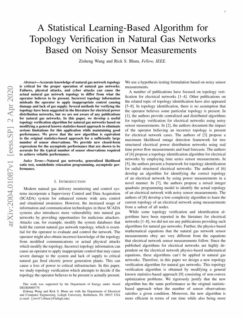
Fig. 1 illustrates a gas distribution system modeled using adirected graph. We allow the topology verification algorithmwe describe in this paper to use pressure, injection/withdraw,and flow measurements. In Fig. 1, these three possible types ofsensors are illustrated. Fig. 1 shows the sensors at node 1 andthe pipeline directly connected to node 1. At the other nodesand pipelines, sensors are employed in the similar way. It is notnecessary to employ all three types of sensors at every nodeor pipeline. We will describe the strategy to employ sensorslater in this paper.

Consider a medium to high pressure network with time-invariant gas injections. The relationship between the gas nodepressures pi, p j and the gas flow φl along the pipeline lconnecting nodes i and j follows the Weymouth equation [11]

αl p2i − p2

j = clφl |φl |, l = 1, . . . ,L (1)

when the graph edge is directed from i to j and αl is the com-pressor ratio in the lth pipeline. Let cl = γl [1− (1−αl)rl ]> 0denote the characteristic value of lth pipelines where γl is thepipeline constant and rl ∈ [0,1] indicates the compressor islocated at normalized distance rl from node i and (1− rl)from node j. When no compressor is present at the lth pipeline,

3

Fig. 1: An example gas distribution network and the corre-sponding directed graph.

αl = 1. The natural gas network satisfies the mass-conservationequation. At each node i, the gas injection qi is equal to thesum of gas flows that leave node i minus the sum of gas flowsthat enter node i, such that

qi = ∑l:leave i

φl− ∑l:enter i

φl , i = 0, · · · ,N (2)

and

q0 =− ∑i∈Ξ,i6=0

qi (3)

where q0 is the injection from the reference node. The refer-ence node is typically chosen as a node supplying gas.

Define ppp , [p1, · · · , pN ]T and qqq , [q1, · · · , qN ]

T . Note thatthe reference node variables p0 and q0 (assumed known) areexcluded from the vectors ppp and qqq. Similarly, we also constructφφφ , [φ1, · · · , φL]

T , ccc , [c1, · · · , cL]T and ααα , [α1, · · · , αL]

T .Based on (1), the L×(N+1) incidence matrix AAA has elements

[AAA]l,n =

+1, n = i+1−1, n = j+10, otherwise

, (4)

with l = 1,2, . . . ,L, n = 0,1, . . . ,N and 0≤ i, j ≤ N. Isolatingthe first column corresponding to the reference node, thematrix AAA can be partitioned as AAA=

[aaa AAA

]. From (2) we obtain

qqq =AAATφφφ which does not involve the reference node. A similarset of manipulations provides a matrix and vector version of(1) that is independent of the reference node, see [11], to obtain

AAATφφφ = qqq, (5)

BBB(ppp ppp) = cccφφφ |φφφ |− p20bbb, (6)

where denotes the element-wise product,

BBB , diagααα[AAA]+− [−AAA]+, (7)

bbb , diagααα[aaa]+− [−aaa]+, (8)

and [x]+ = max(0,x) is an element wise operator.

III. TOPOLOGY VERIFICATION

Let Ψ ⊂ L denote the flow measurements employed byour algorithm. Let Γ ⊂ Ξ denote the pressure measurementsemployed, while Λ ⊂ Ξ denotes the injection/withdraw mea-surements employed. Assume a specific set of pipelines are

changeable such that their states can be open (not employed)or closed (employed). To be completely general, we allow allpipelines to be changeable but in practice this is usually notthe case. Let LC denote the number of changeable pipelines,while φφφC is the vector of flows over these changeable pipelines.The rest of the pipelines are called fixed pipelines. Let LFdenote the number of fixed pipelines, while φφφ F is the vectorof flows over these pipelines. We must have LF +LC = L totalpipelines. We also define four indicator functions that describeif measurements from the uth fixed pipeline, kth changeablepipeline, nth pressure sensor, or nth injection sensor will beemployed as

δF,u =

1, if the uth fixed pipeline ∈Ψ

0, otherwise, (9)

δC,k =

1, if the kth changeable pipeline ∈Ψ

0, otherwise, (10)

δp,n =

1, if the nth pressure sensor ∈ Γ

0, otherwise, (11)

and

δq,n =

1, if the nth injection sensor ∈ Λ

0, otherwise, (12)

with u = 1,2, . . . ,LF ,k = 1,2, . . . ,LC, and n = 1,2, . . . ,N.Let δδδ F = (δF,1, . . . ,δF,LF )

T , δδδC = (δC,1, . . . ,δC,LC)T , δδδ p =

(δp,1, . . . ,δp,N)T ,δδδ q =(δq,1, . . . ,δq,N)

T , δδδ φ =(δδδ TF ,δδδ

TC) and δδδ =

(δδδ TF ,δδδ

TC ,δδδ

Tp ,δδδ

Tq )

T denote the full vector of indicator functions.The following assumptions are made through out this paper.

Assumption 1. The set of all nodes which could be employedis assumed to be known to the operator correctly.

Assumption 2. The set of all measurement errors in the gaspressures, flows and injections/withdraws forms an indepen-dent distributed sequence of zero-mean Gaussian random vari-ables and are not manipulated by attackers. The measurementerrors are taken to be relatively small in this study as theywould be in practice. Larger measurement errors still followthe trends presented.

Assumptions 1 and 2 define our assumed problem model. InSection IV, we provide minimum requirements on the sensorplacement employed. Recall that the matrix AAA describes thetopology of the network when the reference node is excluded.Each row of AAA describes which two nodes are connected bythe pipeline corresponding to the row number as per (4).Let AAAH0 denote the topology describing matrix AAA that theoperator believes is correct. For convenience, we assume thefirst LF rows of AAA, denoted by AAAF , correspond to the fixedpipelines while the next LC rows, denoted by AAAC, correspondto the changeable pipelines. Thus AAA =

[AAAT

F AAATC]T . The same

partition is applied to AAAH0 , aaa, BBB, bbb, and φφφ

In order to verify the topology, we use sensor measurements.At times t = 1,2, · · · ,Ta, we observe noisy versions of thedeterministic gas pressures ppp[t], the injections/withdraws qqq[t],the gas flows over the fixed pipelines φφφ F [t] and the gas flowsover the changeable pipelines φφφC[t]. Let ppp[t],qqq[t],φφφ F [t] and

4

φφφC[t] denote these noisy observations for t = 1,2, · · · ,Ta. ByAssumption 2, at each time t these observations follow ajointly Gaussian distribution with independent components

ppp[t]∼N(ppp,σ2

pIIIN), (13)

qqq[t]∼N(qqq,σ2

q IIIN), (14)

and

φφφ [t] =[φφφ F [t]φφφC[t]

]∼N

([φφφ FφφφC

],σ2

φIIIL

), (15)

where IIIN denotes an N ×N identity matrix, σ2p ,σ

2q and σ2

φ

denote the variances of the measurement errors of the observedgas pressures, withdraws and flows, respectively.

Let PG(xxx|µµµ,ΣΣΣ) denote a Gaussian pdf with the mean vectorµµµ and the covariance matrix ΣΣΣ. Denote the full vector ofobservations as vvv=(ppp[t],φφφ F [t],φφφC[t],qqq[t]) and denote its pdf asg(vvv|θθθ) which is parameterized by θθθ =(vec(AAA)T ,pppT ,φφφ T

F ,φφφTC)

T .Based on Assumption 2 and equations (13)-(15), we have

g(vvv|θθθ) =Ta

∏t=1

N

∏n=1

δδδ p,n 6=0

pG(pppn[t]|pppn,σ2p)

N

∏n=1

δδδ q,n 6=0

pG(qqqn[t]|[AAATφφφ ]n,σ

2q )

LF

∏u=1

δδδ F,u 6=0

pG(φφφ F,u[t]|φφφ F,u,σ2φ )

LC

∏k=1

δδδC,k 6=0

pG(φφφC,k[t]|φφφC,k,σ2φ )

. (16)

To test if the topology matches what the operator believes tobe true (verification), we will test if the observed data comesfrom one of two different possible sets of pdfs. The first setincludes all pdfs g(vvv|θθθ) with θθθ such that AAA =AAAH0 where AAAH0corresponds to the topology the operator expects to be present.The other set includes all other possible pdfs. Due to the factthat the gas pressures and the flows have to follow (6), thenθθθ must satisfy

fff (θθθ) =BBB(ppp ppp)−ccc[φφφ FφφφC

][φφφ FφφφC

]+bbbp2

0 = 000, (17)

in which BBB and bbb were defined in (7) and (8). Define theparameter sets ΘH0 and ΘH1 as

ΘH0 =

θθθ ; fff (θθθ) = 000, AAA =AAAH0

, (18)

and

ΘH1 =

θθθ ; fff (θθθ) = 000, AAA 6=AAAH0

. (19)

Verifying a topology requires solving the following hypoth-esis test involving the family of pdfs g(vvv|θθθ) parameterized byθθθ = (vec(AAA)T , pppT , φφφ T

F , φφφ TC)

T

H0 : θθθ ∈ΘH0 and H1 : θθθ ∈ΘH1 , (20)

where in either case the parameter must satisfy the constraintin (17). Both H0 and H1 are composite hypotheses (more thanone pdf is possible under H0 and H1) which generally makesit much more difficult to define an optimum test [12]. Fora specific set of problems [13], the Generalized LikelihoodRatio Test (GLRT) provides the largest error exponent underH1 such that the probability of error under H1 decreases most

rapidly with more observations. The popular GLRT makes itsdecision by comparing a test statistic to a threshold ρ as

supθθθ∈ΘH1g(vvv|θθθ)

supθθθ∈ΘH0g(vvv|θθθ)

H1≷H0

ρ. (21)

The threshold ρ is typically set to fix the probability thatwe decide for H1 given that H0 is true. This probabilityis called the false alarm probability and denoted by Pf a.The optimizations in (21) are called constrained maximumlikelihood estimates of θθθ . The probability of deciding for H1given H1 is actually true is called the detection probability anddenoted by Pd . The test in (21) is equivalent to

supθθθ∈ΘH1

lng(vvv|θθθ)− supθθθ∈ΘH0

lng(vvv|θθθ)H1≷H0

lnρ, (22)

in which

lng(vvv|θθθ) =C−Ta

∑t=1

12

[1

σ2φ

∥∥∥∥(δδδ FδδδC

)[(

φφφ F [t]φφφC[t]

)−(

φφφ FφφφC

)]∥∥∥∥2

+

1σ2

p

∥∥δδδ p (ppp[t]− ppp)∥∥2

+1

σ2q

∥∥δδδ q(qqq[t]−AAAT

φφφ)∥∥2], (23)

where ‖•‖ denotes the l2 norm, and C =−Ta‖δδδ‖2 ln(2π)/2−Ta‖δδδ q‖2 ln(σq)− (‖δδδ F‖2 +‖δδδC‖2) ln(σφ )−‖δδδ p‖2 ln(σp).

IV. RELAXED GLRT

Due to the optimization problems in (22) being nonconvex,it is difficult to obtain optimal solutions in general. Wecan apply the powerful tool of semidefinite programmingrelaxation (SDR) [14] to change the optimization problemsinvolving continuous variables in (22) to convex problems.This yields a new test. In this section we show the new testachieves a performance which is the same as the performanceof the GLRT test in (22) for the typical values of Ta of interest.We start by defining some quantities to describe the new test.

Define S = N +LF +LC + 1. Let XXX denote an S× S sym-metric positive semidefinite matrix and recall that AAA denotesan L×N matrix of the form defined after (4). All the othervariables employed in the following functions were previouslydefined and are fixed by the physical problem we are solving.Define the functions

g(AAA,XXX ,vvv) =C−Tr(

12

MMM(AAA,vvv)XXX), (24)

and

f (m,AAA,XXX) = Tr(ZZZ(m,AAA)XXX)+bbbm p20, m = 1, . . . ,L, (25)

where Tr(•) denotes the trace operator and

MMM(AAA,vvv) =

MMM′11 000 MMM′13000 MMM′22 MMM′23

MMM′T13 MMM

′T23 MMM′33

, (26)

5

with

MMM′11 = Ta1

σ2p

diag(δδδ p) , (27)

MMM′14 =−Ta

∑t=1

1σ2

pppp[t]δδδ p, (28)

MMM′22 = Ta1

σ2q

AAA diag(δδδ q) AAAT +Ta1

σ2φ

diag(δδδ φ

), (29)

MMM′23 =−Ta

∑t=1

1σ2

qAAA(qqq[t]δδδ q)−

Ta

∑t=1

1σ2

φ

δδδ φ φφφ [t], (30)

and

MMM′33 =Ta

∑t=1

(1

σ2q

∥∥qqq[t]δδδ q∥∥2

+1

σ2p

∥∥ppp[t]δδδ p∥∥2

+

1σ2

φ

∥∥δδδ φ φφφ [t]∥∥2

). (31)

In (25), ZZZ(m,AAA) = diag([

BBB[m,:] −cccmeeem,1×L 0])

where BBB[m,:]denotes the mth row of BBB, and eeem,1×L is an 1×L row vectorwith all zero entries except for the mth which is 1. Let

Ω(AAA) =

XXX ∈ RS×S |XXX ≥ 0; f (m,AAA,XXX) = 0; XXXSS = 1;

XXXT =XXX ; m ∈ 1, · · · ,L

(32)

define a set of values of XXX . Here XXX ≥ 0 implies that XXX ispositive semidefinite. Let AH1 =

AAA |AAA 6=AAAH0

.

Theorem 1 (Standard GLRT Equivalent Expression). Let vvv =(ppp[t],φφφ F [t],φφφC[t],qqq[t]) represent the sensor observations. TheGLRT in (22) can be expressed as

supAAA∈AH1XXX∈Ω(AAA)

rank(XXX)=1

g(AAA,XXX ,vvv)− supXXX∈Ω(AAAH0)rank(XXX)=1

g(AAAH0 ,XXX ,vvv)H1≷H0

lnρ. (33)

Proof. The proof is omitted as it involves only algebra.

The Relaxed GLRT is defined identically to (33) but withthe rank(XXX) = 1 constraint removed.

Definition 1 (Relaxed GLRT). Let vvv = (ppp[t],φφφ F [t],φφφC[t],qqq[t])represent the sensor observations. We define the Relaxed GLRTas the test

supAAA∈AH1XXX∈Ω(AAA)

g(AAA,XXX ,vvv)− supXXX∈Ω(AAAH0)

g(AAAH0 ,XXX ,vvv)H1≷H0

lnρ. (34)

In the sequel, the test in (22) is called the Standard GLRT.The advantage of the Relaxed GLRT is that it can be com-puted in a numerically reliable and efficient manner since theconstraints for the continuous variables are convex. This is nottrue for the Standard GLRT in general due to the nonconvexoptimization problems involved.

One important property of the Relaxed GLRT is that it isequivalent to the Standard GLRT for a sufficiently large Ta,i.e., the optimizations in (34) and (22) yield identical optimalsolutions. Define ωωω = (pppT , φφφ T

F , φφφ TC)

T as the continuous partof θθθ . We define µ(AAA) and ξ (AAA) as

µ(AAA) = supωωω: fff (AAA,ωωω)=000

lng(vvv|ωωω,AAA), (35)

and

ξ (AAA) = supXXX∈Ω(AAA)

g(AAA,XXX ,vvv). (36)

Note that (35) can represent either of the terms in (22) whichare both constrained maximum likelihood (ML) optimizations.Similarly, (36) can stand for either (relaxed) term in (34). Inthe sequel, we call (36) the relaxed ML while (35) is calledthe original ML. From (13)-(15), define

nnnp[t] = ppp[t]− ppp[t]∼N(000,σ2

pIIIN), (37)

nnnq[t] = qqq[t]−qqq[t]∼N(000,σ2

q IIIN), (38)

and

nnnφ [t] = φφφ [t]−φφφ [t]∼N(000,σ2

φIIIL). (39)

The relaxed ML (36) is equivalent to the original one (35),i.e., µ(AAA) = ξ (AAA), for sufficently large Ta.

Theorem 2 (Asymptotic equivalence of the relaxed ML tothe original ML). Suppose that the number of observations Tasatisfies

Ta > max

(∥∥∥∥∥diag(δδδ p)Ta

∑t=1

nnnp[t]

∥∥∥∥∥∞

,

∥∥∥∥∥diag(δδδ φ

) Ta

∑t=1

nnnφ [t]

∥∥∥∥∥∞

,∥∥∥∥∥AAA diag(δδδ q)Ta

∑t=1

nnnq[t]

∥∥∥∥∥∞

/ηmin[AAA diag(δδδ q) AAAT ]) , (40)

where ηmin[AAA diag(δδδ q) AAAT ] denotes the smallest non-zeroeigenvalue of AAA diag(δδδ q) AAAT , and ‖(x1,x2, . . . ,xm)‖∞ =max(|x1|, |x2|, . . . , |xm|) denotes the infinity norm. Then, therelaxed ML (36) is equivalent to the original ML (35), i.e.,µ(AAA) = ξ (AAA). This implies the Relaxed GLRT is equivalent tothe Standard GLRT when Ta satisfies (40) for all possible AAA.

Proof. The proof is shown in Appendix A.

The essence of our proof shows our constrained optimiza-tion problem is a member of a more general class of problemsconsidered in Proposition 5 in [15]. We can also give anintuitive justification to Theorem 2. When we solve eachoptimization in (34) (the relaxed problem) for a sufficientlylarge Ta, the rank of the optimal solution for XXX is always 1.From (26), it can be seen that the deterministic componentsof MMM(AAA,vvv) will be much larger than the random componentsfor a sufficiently large Ta. The dominance becomes even moresignificant as Ta is increased. By ignoring the much smallerrandom parts of MMM(AAA,vvv), the solution to each optimization in(34) (the relaxed problem) is easily shown to be unit rank. Bycomparing Theorem 1 and Definition 1, the rank-1 solutionsare exactly the optimal solutions to each optimization in (33)(the unrelaxed standard problem). Thus the relaxed problemgives the solution for the unrelaxed problem for a sufficientlylarge Ta. In Section VI, we provide numerical results whichshow the rank of XXX is 1 for a sufficiently large Ta for anexample.

6

A. An Efficient Topology Verification Algorithm

The following algorithm is a more efficient way tosolve (20) as opposed to employing (34). Define G =supXXX∈Ω(AAAH0), rank(XXX)=1 g(AAAH0 ,XXX ,vvv).

Step 1: First check if the observed data vvv produces a suf-ficiently small value of G, which implies the data does not fitthe assumed model if H0 is true, so H0 is not true. This allowsus to decide H1 must be true without further calculations. If Gis small, then from (24), infXXX∈Ω(AAAH0)

rank(XXX)=1

Tr( 1

2MMM(AAA,vvv)XXX)

is larger

than zero. Thus, sufficiently small G implies

infXXX∈Ω(AAAH0)rank(XXX)=1

Tr(

12

MMM(AAA,vvv)XXX)> ε, (41)

for a suitable positive ε . Thus we can use (41) to decide H1without further calculations. It is easily shown from Theorem2 that if H0 is true, the left hand side of (41) will approach 0as Ta→∞. Thus (41) will not ever be true if Ta is sufficientlylarge and H0 is true. Thus if (41) is true, we stop and decideH1 is true.

Step 2: If (41) is not true, then we employ (34). We setAAA=AAAH0 and employ the gradient guided search in [16] to solvefor AAA in the first term in (34). The gradient guided search willfirst try all AAA which differ from AAAH0 by a one link change. Itwill pick the one link change that increases the first term in(34) the most. If none of the one link changes increase the firstterm in (34), it will stop and evaluate (34). If it finds a one linkchange that increases the first term of (34), it picks the one linkchange with the largest increase and repeats this procedure. Ifall possible topologies have been tested, the algorithm willstop and evaluate (34).

Now we explain why the algorithm is efficient. If the topol-ogy is changed significantly (true AAA very different from AAAH0 ),then the algorithm will stop during step 1 and no search overthe topology AAA is needed. This will occur when the attackertries to cause significant changes which is typically going tocause significant problems if the operator uses this incorrectnetwork in planning. If the topology undergoes only smallchanges, then the gradient guided search will find the correcttopology quickly. Thus, with appropriate ε , the algorithm willalways stop quickly. We illustrate with numerical results thisand discuss how to pick an appropriate threshold ε in SectionVI.

We end this section by describing a minimum requirementon the sensor placement.

Definition 2 (Proper Sensor Placement). A minimum require-ment for a proper sensor placement for the algorithms givenin Theorem 1 and Definition 1 is that the placement ensuresthe constrained maximum likelihood estimate of θθθ is consistent(converges to the correct value as Ta→ ∞) under hypothesisHi, i ∈ 0,1 when the data used for the estimation is fromHi, i ∈ 0,1.

In the sequel, we consider only sensor placements whichsatisfy Definition 2. At the end of the next section, we providea direct calculation to make sure Definition 2 is satisfied.

V. ASYMPTOTIC PERFORMANCE APPROXIMATION

In this section, we study the asymptotic performances forthe Standard GLRT and the Relaxed GLRT. Define the FisherInformation Matrix (FIM) for estimating ωωω given a general AAAas

JJJ(AAA,ωωω) = Eωωω

[∂

∂ωωωT lng(vvv|AAA,ωωω)∂

∂ωωωlng(vvv|AAA,ωωω)

], (42)

where Eωωω(•) denotes the expected value computed by av-eraging using the pdf in (16) for the assumed value ofωωω . Let FFF(AAA,ωωω) = ∂

∂ωωωfff (AAA,ωωω) where fff (AAA,ωωω) was defined in

(17). Then, for a general AAA define the matrix UUU(AAA,ωωω) ∈R(N+L)×rank(FFF(AAA,ωωω)) as the solution to

FFF(AAA,ωωω)UUU(AAA,ωωω) = 000 such that UUUT (AAA,ωωω)UUU(AAA,ωωω) = III. (43)

Using these definitions, we define the constrained Cramer RaoBound as

CCRB(AAA,ωωω) =UUU(AAA,ωωω)[UUUT (AAA,ωωω)

JJJ(AAA,ωωω)UUU(AAA,ωωω)]−1UUUT (AAA,ωωω). (44)

Lemma 1. Let θθθ∗ = (vec(AAA∗) ,ωωω∗)T be the solution to

supθθθ∈ΘH1lng(vvv|θθθ) when the data vvv is obtained under H1 from

a network with a topology described by AAAH1 with the noisefree network variables ωωωH1 = (pppT

H1, φφφ T

H1,F , φφφ TH1,C)

T . GivenDefinition 2, θθθ

∗ approaches (vec(AAAH1) ,ωωωH1)T as Ta → ∞.

This implies that the probability that AAA∗ 6= AAAH1 goes to 0 asTa→ ∞.

The proof follows from the definition of consistency. Thusfor Ta→ ∞, all the estimates must be exactly the true valuesin the system.

Lemma 2. For the case in Lemma 1, for a sufficiently large butfinite Ta, the probability that AAA∗ 6=AAAH1 can be made arbitraryclose to zero.

Proof. Based on the Karush Kuhn Tucker (KKT) conditionswe can show that if AAA = AAAH1 , all the elements of ωωω∗ areunbiased and their variances are inversely proportional to Ta.Thus considering φφφ ∗ when AAA =AAAH1 , we can show

Eφφφ ∗= [σ2φAAA diag(δδδ q) AAAT +σ

2q diag

(δδδ φ

)]†

[σ2φAAA diag(δδδ q) AAA+σ

2q diag

(δδδ φ

)]φφφ H1 = φφφ H1 , (45)

and

Cov[φφφ ∗] =σ2

φσ2

q

Ta[σ2

φAAAdiag(δδδ q)AAAT +σ2q diag

(δδδ φ

)]†T . (46)

We can show similar equations for the other elements ofωωω∗. Now if AAA 6= AAAH1 , the KKT conditions show that all theelements of ωωω∗ are biased and still their variance are inverselyproportional to Ta.

When AAA = AAAH1 , all the scalar parameter estimates of thecomponents of ωωω , other than AAA, are unbiased and the varianceof each parameter estimate becomes smaller as Ta increases.Thus, the parameter estimates get better and better as Ta in-creases since their distribution becomes more closely focusedaround the correct value. This makes all the squared normterms in lng(vvv|θθθ) in (23) very close to zero so the likelihood

7

g(vvv|θθθ) is as large as it can be. Note that the squared normterm involving qqq[t] in lng(vvv|θθθ) is also a narrow Gaussiancentered on zero (becoming more narrow as Ta increases) sothe argument to this square norm is also very close to zero.This is what happens if AAA =AAAH1 .

Now if AAA 6=AAAH1 , then the mean vector of the estimate of ωωω

will be biased and the arguments to the squared norm termsof lng(vvv|θθθ) in (23) are also biased and again these terms areGaussian. Now as Ta is increased the variances of each ofthese terms will decrease so the distribution becomes moreclosely focused around an incorrect value. At a large enoughTa, the squared error in these term with bias (AAA 6=AAAH1 ) will bebe much larger than the unbiased error in the estimates whenAAA=AAAH1 and all the variances are small. In fact at large enoughTa, the overlap between the probability density functions of thebiased terms and the unbiased terms will be small and we canmake this overlap as small as we like by increasing Ta. Thismakes the probability that the likelihood with AAA=AAAH1 is largerthan that with AAA 6=AAAH1 true with a probability near unity whichwe can make as close as we like to unity by increasing Ta.This completes the proof.

Based on Lemma 2, under H1 we must have AAA∗ = AAAH1with high probability for sufficiently large Ta so (22) isasymptotically equivalent with high probability to

supωωω∈Aω1

lng(vvv|AAAH1 ,ωωω)− supωωω∈Aω0

lng(vvv|AAAH0 ,ωωω)H1≷H0

lnρ. (47)

in which Aωi = ωωω : f (AAAHi ,ωωω) = 000 , i ∈ 0,1. Further sim-plification results by using the fact that such a test is asymptot-ically equivalent to the corresponding Wald test as describedin the following theorem.

Theorem 3. Under H1, for Ta→ ∞ the test in (47) becomesequivalent to the test[

ωωω−ωωω∗ (AAAH0

)]T CCRB† (AAAH0 ,ωωω∗ (AAAH0

))[ωωω−ωωω

∗ (AAAH0

)] H1≷H0

lnρ, (48)

where CCRB† (AAAH0 ,ωωω∗ (AAAH0

))denotes the pseudo-inverse of

(44), ωωω = argsupω∈Aω1lng(vvv|AAAH1 ,ωωω), and ρ is chosen to fix

the false alarm probability.

Proof. The proof follows from the result in [17] combinedwith Appendix 6A in [18].

The following lemma describes the distribution of (48).

Lemma 3 (Distribution of (48)). Define λ = [ωωω∗(AAAH1)− ωωω∗

(AAAH0

)]T CCRB†(AAAH0 ,ωωω

∗(AAAH1))[ωωω∗(AAAH1)−ωωω∗

(AAAH0

)].

Then, under H1 the test statistic in (48) asymptotically (largeTa) follows the non-central chi-squared distribution withL+N degrees of the freedom and non-centrality parameterλ .

Proof. The proof is shown in Appendix 6C in [18].

Define the Marcum Q function with w degrees of freedom[19] as

Qw(a,b) =∫

∞

bx( x

a

)w−1exp(−x2 +a2

2

)Iw−1(ax)dx (49)

where Iw−1(x) is the modified Bessel function of order w−1. Then the inverse of the Marcum Q function Q−1

w (c,d) isdefined as the solution y to Qw(c,y) = d [20]. The followingtheorem employs Lemma 3 to describe the performance of theStandard GLRT for large T .

Theorem 4 (Asymptotic Performance Approximation of theStandard GLRT). For a sufficiently large Ta and a fixed falsealarm probability Pf a, an accurate expression for the detectionprobability for the Standard GLRT is

Pd = QL+N(√

λ ,√

ρ) (50)

where ρ = Q−1L+N(0,Pf a), UUU =UUU(AAAH0 ,ωωω

∗ (AAAH0

)) was defined

in (43),

λ =[ωωω∗(AAAH1)−ωωω

∗ (AAAH0

)]TUUUUUUTJJJ(AAAH0

)UUUUUUT[

ωωω∗(AAAH1)−ωωω

∗(AAAH0)], (51)

and (42) yields

JJJ(AAAH0

)= Ta

[JJJ′pp 000000 JJJ′

φφ

(AAAH0

)] , (52)

where the sub-matrices of JJJ(AAAH0

)are

JJJ′pp =1

σ2p

diag(δδδ p) , (53)

JJJ′φφ

(AAAH0

)=

1σ2

φ

diag(δδδ φ

)+

1σ2

qAAAH0diag(δδδ q)AAAT

H0. (54)

Note that Pd in (50) increases monotonically with Ta.

Proof. Using Lemma 3, under H1 the test in (22) asymp-totically follows the non-central chi-squared distribution withL+N degrees of freedom and the non-centrality parameter

λ =[ωωω∗(AAAH1)−ωωω

∗(AAAH0)]T UUU

[UUUTJJJ(AAAH0)UUU

]−1UUUT†[

ωωω∗(AAAH1)−ωωω

∗(AAAH0)], (55)

To resolve the pseudo inverse, note that (EEEEEET )† =

EEE(EEETEEE)−2EEET . Let EEE =UUU[UUUTJJJ(AAAH0)UUU

]−1/2 then we have

λ =[ωωω∗(AAAH1)−ωωω

∗(AAAH0)]TUUUUUUTJJJ(AAAH0)UUUUUUT[

ωωω∗(AAAH1)−ωωω

∗(AAAH0)]. (56)

From Theorem 2, the Relaxed GLRT is asymptoticallyequivalent to the Standard GLRT. Thus to derive the asymp-totic performance of the Relaxed GLRT, we just need to cal-culate the ωωω∗(AAA) corresponding to the optimal XXX∗(AAA) obtainedfrom (36). Using (32) and equating the solution of (33) to (34)(with significant algebra) when (40) is satisfied

XXX∗(AAA) =[ωωω∗(AAA)

1

][ωωω∗T (AAA) 1

]. (57)

8

Given the definitions of S and XXX before (26), the solution,called ωωω

∗(AAA), is [ωωω∗(AAA)1

]=XXX∗[:,S](AAA). (58)

in which XXX∗[:,S](AAA) is Sth column of XXX∗(AAA). Therefore, theasymptotic performance of the Relaxed GLRT under H1can be obtained by substituting ωωω

∗(AAAH1) into the asymptoticperformance of the Standard GLRT shown in Theorem 4.

Next we provide a simplied sensor placement procedure. LetAAAopen denote the incidence matrix as per (4) for the topologywith all changeable pipelines opened. Similarly, we have BBBopendefined using the conventions in (7).

Theorem 5 (Simplified Proper Sensor Placement). DefineFFF(AAA) = [BBB diag(ccc)]. Let UUU(AAA) = [IIIN −BBBT diag−1(ccc)]T . Therequirement of Definition 2 will be guaranteed if

rank[UUU

T(AAAopen)JJJ (AAAopen)UUU(AAAopen)

]= N. (59)

Proof. Based on Theorem 2 in [21], for a general AAA, to satisfythe requirement of Definition 2, we need

rank[UUUT (AAA,ωωω∗ (AAA))JJJ (AAA)UUU (AAA,ωωω∗ (AAA))

]=

S− rankFFF (AAA,ωωω∗ (AAA))−1. (60)

Recall that ωωω∗ = [ppp∗T φφφ ∗T ]T . By taking the partial derivativeof fff (AAA,ωωω) with respect to ωωω , we have

FFF (AAA,ωωω∗ (AAA)) =[2BBB diag(ppp∗) 2diag(cccφφφ ∗)

]= FFF(AAA) diag(2ωωω

∗ (AAA)) . (61)

where the ranks of FFF (AAA,ωωω∗ (AAA)) and FFF(AAA) are both L sincecccl > 0, l = 1, . . . ,L as per (1).

Define a square non-singular matrix PPP ∈ RN×N such thatUUU (AAA,ωωω∗ (AAA)) =UUU(AAA)PPP. This matrix PPP exists since the columnsof both UUU (AAA,ωωω∗ (AAA)) and UUU(AAA) are individually a basis for thenull space of FFF(AAA). Then, we have

rank[UUUT (AAA,ωωω∗ (AAA))JJJ (AAA)UUU (AAA,ωωω∗ (AAA))

]= rank

[PPPTUUU(AAA)TJJJ (AAA)UUU(AAA)PPP

]= rank

[UUU

T(AAA)JJJ (AAA)UUU(AAA)

]. (62)

By (52)-(54) and the definition of UUU(AAA), we have

UUUT(AAA)JJJ (AAA)UUU(AAA) =

1σ2

φ

BBBT diag−1(ccc)diag(δδδ φ

)diag−1(ccc)BBB+

1σ2

φ

BBBT diag−1(ccc)AAA diag(δδδ q) AAAT diag−1(ccc)BBB+1

σ2p

diag(δδδ p) .

(63)

The first term of the right hand side of (63) is the weightedLaplacian matrix (edges are weighted by ccc and δδδ φ ) whilethe 2nd term has the same rank as the weighted Lapla-cian matrix. Connecting any unconnected links will in-crease or maintain the rank of a Laplacian matrix (Sec-tion 2 in [? ]). Thus, rank

[UUU

T(AAAopen)JJJ

(AAAopen

)UUU(AAAopen)

]≤

rank[UUU

T(AAA)JJJ (AAA)UUU(AAA)

]. Hence, if (59) is true for AAAopen, then

(a) (b)

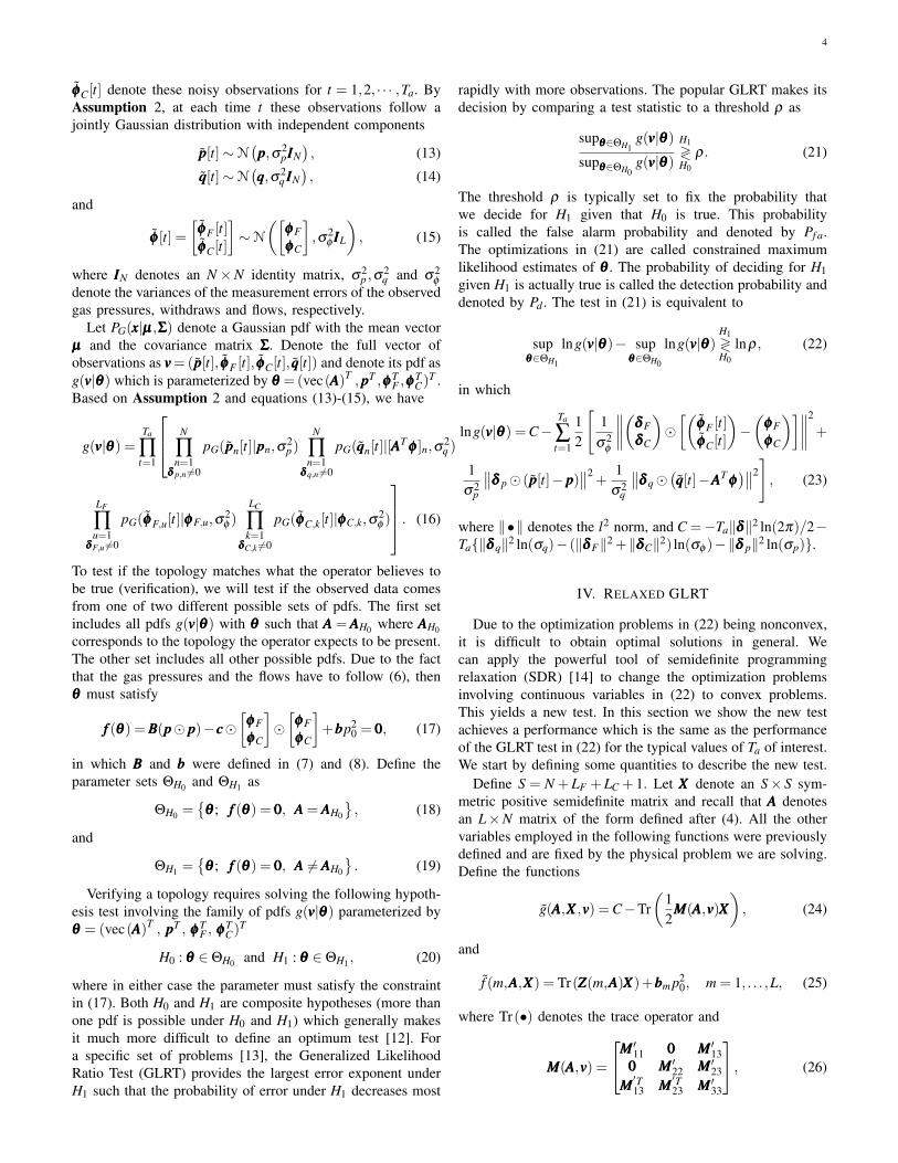
Fig. 2: Natural gas networks evaluated in this paper. Dashedlines indicate changeable pipelines while solid lines are fixedpipelines. Blue nodes involve withdraws of gas from networkswhere as the green node involves the injection of gas intonetworks. (a) Network 1 [22] (b) Network 2 [23].

TABLE II: Changeable pipeline settings under H0/H1 for 4different cases in Network 1

Changeable pipeline states (H0/H1)Case C1 C2 C3

Case 1 Closed/Closed Closed/Closed Closed/OpenCase 2 Open/Open Closed/Closed Open/ClosedCase 3 Closed/Closed Closed/Closed Open/ClosedCase 4 Open/Closed Open/Closed Open/Closed

(59) must be true for all AAA obtained from AAAopen by closingchangeable pipelines.

We first define an optimal placement as a placement whichsatisfies Definition 2 while having the lowest cost. We can findthe optimal placement by solving

minδδδ

N

∑n=1

(dp,nδp,n +dq,nδq,n)+LF

∑l=1

dF,lδF,l +LC

∑k=1

dC,kδC,k, (64)

subject to: (59), (65)

where dp,n and dq,n are costs for placing pressure and injectionsensors at the nth node respectively, and dF,l and dC,l are costsfor placing flow meters at the lth pipeline, respectively. Solving(64) and (65) is hard since (59) is not linear.

Thus we describe a practical approach to find a placementwhich is simple and typically provides acceptable cost (notso much more than optimum) based on our numerical inves-tigations, some given in this paper. First note that placing apressure sensor at every node always satisfies Definition 2.This can be easily proved by substituting δδδ p = 111 into (59).Then, we can try to remove an arbitrary sensor from theplacement and add another sensor which has a lower costand allows a new placement which satisfies (59). We repeatthis procedure until the cost cannot be further decreased.Based on (59), the minimum number of placed sensors is N.Thus, our starting point δδδ p = 111 uses this minimum numberof sensors. Since the replacing step only deceases the totalcost, the final solution can only be closer to the optimal. Thisapproach is efficient since it starts at a point with the minimumnumber of sensors and trys to exchange sensors to reduce cost.We provide numerical results for this placement approach inSection VI.

VI. NUMERICAL RESULTS

In this section, we evaluate the performance of the RelaxedGLRT. To this end, we consider two natural gas networks

9

TABLE III: Changeable pipeline settings under H0/H1 for 2different cases in Network 2

Changeable pipeline states (H0/H1)Case C1 C2 C3 C4

Case 1 Closed/Closed Closed/Closed Closed/Closed Closed/OpenCase 2 Closed/Open Closed/Closed Closed/Closed Closed/Open

TABLE IV: Gas injections and pipeline characteristic valuesused in numerical investigations.

Network 1 Network 2Node qqq Pipe. ccc Node qqq Pipe. ccc

0 223 L1-L13 12 0 183 L1− L11 121-7 −20 C1-C3 12 1-3,12,13 −20 C1−C4 128-13 −8 4-6 −8

8-11 −6.5

The unit of qqq is [m3/s]. The unit of ccc is [kg2m−8s−2]

in this paper. Fig. 2a shows one 14-node natural gas network[22], called Network 1 while Fig. 2b presents another 14-nodenatural gas network [23], called Network 2. Pipelines markedC (in Network 1) or C (in Network 2) are changeable pipelineswhile the others are fixed. Table II describes the states ofchangeable pipelines that the operator believes to be present(H0) along with the actual pipeline settings (H1) in threedifferent cases (Cases 1-4) of Network 1. Table III describesthe states of changeable pipelines in two cases (Cases 1 and 2)of Network 2. Table IV describes the gas injections/withdrawsand the pipeline characteristic values used in our numericalinvestigations for both networks, which are fixed regardless ofthe changeable pipeline settings. Table V describes the actualgas flows for each pipeline under H0 and H1 for Network 1while Table VI describes these flows for Network 2. Table VIIand Table VIII describe the directions of gas flows under H0for Network 1 and Network 2, respectively. For Cases 1-4 ofNetwork 1 under H1, the direction of the flow of L4 is from 6

TABLE V: Pipeline gas flows for Cases 1-3 of Network 1under H0 and H1

Flows for each case [m3/s].

H1 H1 H1 H0 H0 H0

Pipe. Case 1 Case 2 Case 3 Case 1 Case 2 Case 3

L1 223.0 223.0 223.0 223.0 223.0 223.0L2 100.0 100.0 100.0 100.0 100.0 100.0L3 75.0 75.0 75.0 75.0 75.0 75.0L4 50.0 50.0 50.0 50.0 50.0 50.0L5 25.0 25.0 25.0 25.0 25.0 25.0L6 98.0 98.0 98.0 98.0 98.0 98.0L7 73.0 73.0 73.0 73.0 73.0 73.0L8 48.0 48.0 48.0 48.0 48.0 48.0L9 20.4 20.0 21.4 21.4 19.2 20.4L10 6.2 12.0 6.7 6.7 11.2 6.2L11 4.4 0.0 0.9 0.9 3.2 4.4L12 8.0 4.0 3.5 3.5 8.0 8.0L13 19.5 20.0 18.5 18.5 20.8 19.5

TABLE VI: Pipeline gas flows for Cases 1 and 2 of Network2 under H0 and H1

Flows for each case [m3/s]

H1 H1 H0 H1 H1 H0

Pipe. Case 1 Case 2 Cases Pipe. Case 1 Case 2 Cases

L1 183.0 183.0 183.0 L7 6.5 6.5 7.9L2 79.4 82.0 79.2 L8 19.5 19.5 20.9L3 54.4 57.0 54.2 L9 28.5 26.0 28.7L4 29.4 32.0 29.2 L10 53.5 51.0 53.7L5 24.0 24.0 22.5 L11 78.5 76.0 78.7L6 8.0 8.0 6.5

TABLE VII: Directions of pipelines flows under H0 for Cases1-3 of Network 1

Pipeline Start End Pipeline Start endNum. Node Node Num. Node Node

L1 0 1 L9 8 9L2 1 2 L10 8 10L3 2 5 L11 9 11L4 5 6 L12 11 12L5 6 7 L13 12 13L6 1 2 C1 1 4L7 3 4 C2 3 6L8 4 8 C3 5 8

to 5, while the others are the same as in Table VII. For Cases1 and 2 of Network 2 under H1, the direction of the flow ofL7 is from 8 to 9, while the others are the same as in TableVIII. The relative size of the noise for each sensor is describedusing the relative standard derivation (RSD) τ = σ/µ whereσ and µ are the standard derivation and the mean of thenoisy measurement. RSD is often quoted as a percentage.We assume that each sensor has the same RSD. Our resultsassume pressure and injection/withdraw sensors at all nodesas well as flow sensors on all fixed pipelines to collect noisymeasurements of pressures, injections/withdrawns, and flows.The metric we use to quantify the performance is the detectionprobability under 0.1% false alarm probability for a givenRSD.

If the detection probability is higher than 99.9% in aspecific case, we declare that the Relaxed GLRT obtains

TABLE VIII: Directions of pipelines flows under H0 for Cases1 and 2 of Network 2

Pipeline Start End Pipeline Start endNum. Node Node Num. Node Node

L1 0 1 L9 12 11L2 1 2 L10 13 12L3 2 3 L11 1 13L4 3 4 C1 4 11L5 4 5 C2 10 4L6 6 7 C3 5 6L7 9 8 C4 7 8L8 11 10

10

4 4.5 5 5.5 6 6.5 7 7.5 8 8.5 9

RSD (%)

99

99.2

99.4

99.6

99.8

100

Pd (

dete

ctio

n pr

obab

ility

) (%

)

Ta = 35

Ta = 40

Ta = 45

(a)

2 2.5 3 3.5 4 4.5 5 5.5 6 6.5 7

RSD (%)

99

99.2

99.4

99.6

99.8

100

Pd (

dete

ctio

n pr

obab

ility

) (%

)

Ta = 65

Ta = 70

Ta = 75

(b)

Fig. 3: Simulated Pd under different RSD values. (a) Case 1,Network 1; (b) Case 1, Network 2.

60 70 80 90 100 110 120

Ta

99

99.2

99.4

99.6

99.8

100

Pd (

dete

ctio

n pr

obab

ility

) (%

)

Case 1Case 2Case 3

(a)

40 60 80 100 120 140 160

Ta

99

99.2

99.4

99.6

99.8

100

Pd (

dete

ctio

n pr

obab

ility

) (%

)

Case 1Case 2

(b)

Fig. 4: Simulated Pd of all cases. (a) Cases 1-3, Network 1with 10% RSD; (b) Cases 1 and 2, Network 2 with 8% RSD.

reliable performance for that case. We employed Monte-Carlosimulations using 105 runs.

In Fig. 3, we study Pd versus the RSD for Case 1 ofNetwork 1 and Case 1 of Network 2. Fig. 3 shows that Pdincreases as the RSD decreases. For different Ta, the RSDrequired to obtain good performance is also different. ForTa = 35,40,45 and Case 1 of Network 1, the Relaxed GLRTprovides good performance when RSD is lower than 6.6%,7%and 7.5%, respectively. Moreover, Fig. 4 shows the Pd ofall cases described in Tables II and III. We observe that theRelaxed GLRT will always obtain good performance with asufficiently large Ta. The minimum number of observationsneeded to obtain good performance for all cases is listed inthe third row of Table IX.

Next, we evaluated the minimum Ta to achieve good per-formance for the three cases under Network 1 and for the twocases under Network 2 and we listed these values of Ta in

TABLE IX: The detection probability Pd of simulations andthe asymptotic performance for all cases

Network 1 Network 2Case 1 Case 2 Case 3 Case 1 Case 2

Min. Ta 80 100 80 114 47Pd (Simu.) 99.90% 99.89% 99.90% 99.89% 99.89%Pd (Asymp.) 99.65% 99.85% 99.65% 99.87% 99.94%Pd Diff. 0.25% 0.04% 0.25% 0.02% 0.05%

10% RSD for Network 1; 8% RSD for Network 2.

70 75 80 85 90 95 100 105 110 115 120

Ta

99.4

99.5

99.6

99.7

99.8

99.9

100

Pd (

dete

ctio

n pr

obab

ility

) (%

)

Simulated PerformanceAsymptotic Approximation

(a)

90 95 100 105 110 115 120

Ta

99.4

99.5

99.6

99.7

99.8

99.9

100

Pd (

dete

ctio

n pr

obab

ility

) (%

)

Simulated PerformanceAsymptotic Approximation

(b)

70 75 80 85 90 95 100 105 110 115 120

Ta

99

99.2

99.4

99.6

99.8

100

Pd (

dete

ctio

n pr

obab

ility

) (%

)

Simulated PerformanceAsymptotic Approximation

(c)

Fig. 5: Asymptotic performances of the Relaxed GLRT com-pares to the simulated Pd . (a) Case 1, Network 1; (b) Case 2,Network 1; (c) Case 3, Network 1.

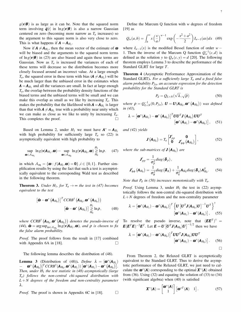
Table IX. Table IX also lists both the asymptotic performancedefined in Theorem 4 for Pd and the simulated Pd for thesecases. These results show that the asymptotic performance isaccurate for the value of Ta listed in Table IX which implygood performance. In particular, we see that for the given valueof Ta, the difference between the asymptotic performanceand the simulated Pd is less than 0.25% for all evaluatedcases. Additionally, if we use an even larger value of Ta, asshown in the yellow zones in Figures 5 and 6, the asymptoticperformance is closer to the simulated performance.

We give numerical result to verify that the solution to eachoptimization in (33) (the relaxed problem) is unit rank basedon (24) and (26) for a sufficiently large Ta. For this numericalinvestigation, when an eigenvalue is smaller than 10−4, weregard it as zero. Fig. 7 shows the rank of the optimal XXX(number of non-zero eigenvalues) for Network 1 in Case 1

11

100 110 120 130 140 150 160

Ta

99.5

99.6

99.7

99.8

99.9

100

Pd (

dete

ctio

n pr

obab

ility

) (%

)

Simulated PerformanceAsymptotic Approximation

(a)

35 40 45 50 55 60 65 70 75 80

Ta

99.4

99.5

99.6

99.7

99.8

99.9

100

Pd (

dete

ctio

n pr

obab

ility

) (%

)

Simulated PerformanceAsymptotic Approximation

(b)

Fig. 6: Asymptotic performances of the Relaxed GLRT com-pares to the simulated Pd . (a) Case 1, Network 2; (b) Case 2,Network 2.

20 40 60 80 100 120 140 160

Ta

0

2

4

6

8

10

12

14

Ran

k of

X

Network 1 Case 1Network 1 Case 2

Fig. 7: The rank of the optimal XXX for Network 1 Case 1 and2.

and 2 with 5% RSD. Fig. 7 shows that the rank of the optimalXXX is always 1 for Ta > 100.

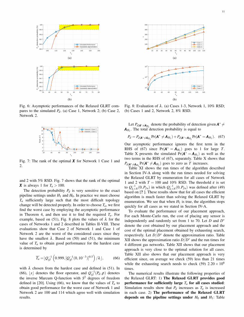
The detection probability Pd is very sensitive to the exactpipeline settings under H1 and H0. In practice we must chooseTa sufficiently large such that the most difficult topologychange will be detected properly. In order to choose Ta, we firstfind the worst case by employing the asymptotic performancein Theorem 4, and then use it to find the required Ta. Forexample, based on (51), Fig. 8 plots the values of λ for thecases of Networks 1 and 2 described in Tables II-VIII. Theseevaluations show that Case 2 of Network 1 and Case 1 ofNetwork 2 are the worst of the considered cases since theyhave the smallest λ . Based on (50) and (51), the minimumvalue of Ta to obtain good performance for the hardest caseis determined by

Ta =bQ−1S2

(0.999, [Q−1

S2 (0,10−3)]0.5)/λc, (66)

with λ chosen from the hardest case and defined in (51). In(66), bxc denotes the floor operator, and Q−1

S2 (Pd ,ρ) denotesthe inverse Marcum Q-function with S2 degrees of freedomdefined in [20]. Using (66), we know that the values of Ta toobtain good performance for the worst case of Network 1 andNetwork 2 are 100 and 114 which agree well with simulationresults.

10 20 30 40 50 60 70 80 90 100 110 120

Ta

0

100

200

300

400

500

Case 1Case 2Case 3

(a)

20 40 60 80 100 120 140 160

Ta

101

102

103

Case 1Case 2

(b)

Fig. 8: Evaluation of λ . (a) Cases 1-3, Network 1, 10% RSD;(b) Cases 1 and 2, Network 2, 8% RSD.

Let Pd|AAA∗ 6=AAAH1denote the probability of detection given AAA∗ 6=

AAAH1 . The total detection probability is equal to

Pd = Pd|AAA∗ 6=AAAH1Pr(AAA∗ 6=AAAH1)+Pd|AAA∗=AAAH1

Pr(AAA∗ =AAAH1). (67)

Our asymptotic performance ignores the first term in theRHS of (67) since Pr(AAA∗ = AAAH1) goes to 1 for large T .Table X presents the simulated Pr(AAA∗ = AAAH1) as well as thetwo terms in the RHS of (67), separately. Table X shows thatPd|AAA∗ 6=AAAH1

Pr(AAA∗ 6=AAAH1) goes to zero as T increases.Table XI shows the run times of the algorithm described

in Section IV-A along with the run times needed for solvingthe Relaxed GLRT by enumeration for all cases of Network1 and 2 with T = 100 and 10% RSD. The threshold ε is setto Q−1

L+N(0,Pf a) in which Q−1L+N(0,Pf a) was defined after (49)

based on [? ]. These results show that for all cases the efficientalgorithm is much faster than solving the Relaxed GLRT byenumeration. We see that when H1 is true, the algorithm stopsquickly for all cases as we stated in Section IV-A.

To evaluate the performance of our placement approach,For each Monte-Carlo run, the cost of placing any sensor isindependently and randomly set from 1 to 70. Let D and D∗

denote the cost obtained by our placement approach and thecost of the optimal placement obtained by exhausting search,respectively. Let D/D∗ denote the approximation ratio. TableXII shows the approximation ratio D/D∗ and the run times for4 different gas networks. Table XII shows that our placementapproach is very close to the optimal solution for all cases.Table XII also shows that our placement approach is veryefficient since, on average we check (59) less than 21 timeswhile the exhausting search needs to check (59) 2.20× 106

times.The numerical results illustrate the following properties of

the Relaxed GLRT: 1) The Relaxed GLRT provides goodperformance for sufficiently large Ta for all cases studied:Simulation results show that Pd increases as Ta is increasedin each case. 2) The performance of the Relaxed GLRTdepends on the pipeline settings under H0 and H1: Table

12

TABLE X: The probability of AAA =AAAH1 and corresponding Pd .

Pipeline Setting Ta 50 60 70 80 90 100

Network 1 Pd|AAA∗ 6=AAAH1Pr(AAA∗ 6=AAAH1 ) 0.0069% 0.0013% 0.0002% < 0.0001% < 0.0001% < 0.0001%

Case 1 Pd|AAA∗=AAAH1Pr(AAA∗ =AAAH1 ) 98.11% 99.12% 99.62% 99.74% 99.84% 99.99%

RSD= 10% Pr(AAA∗ =AAAH1 ) 99.16% 99.64% 99.86% 99.92% 99.94% 99.99%

Network 1 Pd|AAA∗ 6=AAAH1Pr(AAA∗ 6=AAAH1 ) 0.42% 0.06% 0.03% 0.01% 0.01% 0.01%

Case 2 Pd|AAA∗=AAAH1Pr(AAA∗ =AAAH1 ) 98.49% 99.38% 99.58% 99.76% 99.86% 99.98%

RSD= 10% Pr(AAA∗ =AAAH1 ) 99.34% 99.74% 99.82% 99.90% 99.92% 99.99%

TABLE XI: The average run times of the algorithm

Network 1 Network 2Case 1 Case 2 Case 3 Case 4 Case 1 Case 2

H0 true 2.56s 2.89s 2.01s 3.44s 2.80s 1.57sH1 true 0.54s 0.62s 1.48s 0.64s 1.43s 0.62sEnum. 5.30s 5.56s 4.14s 5.36s 9.76s 9.84s

TABLE XII: The performance of our placement approach fordifferent networks.

Networks0 1

2 3 4

5

6 7 8

01

2 3 4

5

6 7 8

0 1 2 3

4

56 7 8

0

1 2 3

4

56

D/D∗ 1.1398 1.2263 1.1224 1.2703Run time 0.1438s 0.1945s 0.1586s 0.1655s

Exhausting search takes 2123.70s .

IX shows that Pd varies for different cases and networksgiven fixed Ta. 3) The asymptotic performance proposedin Theorem 4 is accurate for the values of Ta needed toachieve good performance. 4) In cases where we requiregood performance, we use λ to find out the most difficultpipeline change to detect, then the required number ofobservations to achieve good performance is given by (66).

VII. CONCLUSIONS AND DISCUSSION

In this paper, we describe a new algorithm for employingsensor measurements to perform topology verification of nat-ural gas networks. Our algorithm is based on relaxing someoptimization problems in the classical statistical hypothesistesting approach called the GLRT. The GLRT generally workswell when the optimization problems involved in computingit are convex, but it is difficult to guarantee good performancewhen some of the optimization problems are nonconvex. How-ever, in our application the GLRT will involve some nonconvexoptimizations that correspond to estimating some continuousvalued parameters describing the mathematical models ofsome pressures and flows in the natural gas network. Ournew algorithm removed some constraints to produce convexoptimizations for the estimation of these continuous valuedvariables, while ensuring identical performance to the GLRTfor an appropriate number of sensor observations. Hence, ournew algorithm is much efficient and reliable since solving itonly involves convex optimization programming. We derivenew closed-form expressions for the asymptotic performanceof our algorithm in terms of the probability of detection. Wehave not seen any derivations in the literature of the asymptotic

performance for the cases we consider here in this paper,which involve estimations of discrete variables which describethe natural gas network topology. The asymptotic resultsalso describe the required number of observations neededto achieve reliable performance. We also provide sufficientconditions for an appropriate sensor placement. The approachemployed to derive the closed-form asymptotic performanceexpressions is pretty general and can be used to solve anyGLRT which involves both continuous and discrete quantitiesthat must be estimated or any modified GLRT which usesrelaxed versions of the optimizations employing these estima-tions.

As this is the first paper on this topic of topology verifi-cation of natural gas networks, we focus on the most basicsetting. For example, we do not consider cases where thesensors may fail and give faulty measurements or where thecommunications which send the sensor data may fail. Wealso do not consider cases where the sensor measurementsmight be manipulated by attackers. We intend to study thesecases in future work. The baseline provided in this paperis very helpful as a start for such work, since it describesvery favorable performance with no attacks or failures. Ifwe can find acceptable complexity topology identificationapproaches which can identify attacks and failures and usethis information to appropriately process the compromisedand uncompromised data to achieve performance close to theunattacked performance, see [24], then these approaches willbe very useful for practical deployment.

APPENDIX ATHE PROOF OF THEOREM 2: ASYMPTOTIC EQUIVALENCE

OF THE RELAXED ML TO THE ORIGINAL ML

Define a function h : RS×S → RS by h(XXX) =[XXX1,1 XXX2,2 . . . XXXS,S

]T . In the relaxed ML (36), theconstraints f (m,AAA,XXX) = Tr(ZZZ(m,AAA)XXX) + bbbm p2

0 confine onlydiagonal elements of XXX , because ZZZ(m,AAA) is a diagonal matrixwhich was defined as

ZZZ(m,AAA) = diag([

BBB[m,:] −cccmeeem,1×L 0]). (68)

where m= 1, . . . ,L, BBB[m,:] denotes the mth row of BBB, cccm denotesmth entry of the pipeline characteristic vector ccc, and eeem,1×Lis an 1× L row vector with all zero entries except for the

13

mth which is 1. Then, the diagonal elements of XXX live in thesolution space of the following linear equations f (1,AAA,XXX)

...f (L,AAA,XXX)

= 000. (69)

Let Π(AAA) = h(XXX)| f (m,AAA,XXX) = 0,m = 1, . . . ,L. Then, therelaxed ML (36) becomes

ξ (AAA) = suph(XXX)∈Π(AAA), XXX≥0, XXX=XXXT

C−Tr(MMM(AAA,vvv)XXX) . (70)

Define 111 as an all one column vector whose the dimen-sion is equal to the number of observations. Define thevectors δδδ p = 111⊗ δδδ p, δδδ q = 111⊗ δδδ q, δδδ φ = 111⊗

[δδδ T

F δδδ TC]T ,

IIIL = 111⊗ IIIL, IIIN = 111⊗ IIIN , and AAA = 111⊗AAAT where ⊗ denotesthe kronecker product. Define the full observation vectorsas ppp = (pppT [1], · · · , pppT [Ta])

T , qqq = (qqqT [1], · · · ,qqqT [Ta])T , and

φφφ =(φφφT[1], · · · ,φφφ T

[Ta])T . Define the full noise vectors as nnnp =

(nnnTp [1], · · · , nnnT

p [Ta])T , nnnq = (nnnT

q [1], · · · , nnnTq [Ta])

T , and nnnφ =(nnnT

φ[1], · · · , nnnT

φ[Ta])

T . Then, the original ML (35) becomes

µ(AAA) = supωωωωωω∈Π(AAA)

C− 12

[∥∥∥∥ 1σφ

δδδ φ (φφφ −IIILφφφ

)∥∥∥∥2

+

∥∥∥∥ 1σq

δδδ q(qqq−AAAφφφ

)∥∥∥∥2

+

∥∥∥∥ 1σp

δδδ p(ppp−IIIN ppp

)∥∥∥∥2]. (71)

Proposition 5 in [15] shows that µ(AAA) = ξ (AAA) when thefollowing conditions are satisfied simultaneously

ηmin

[IIIT diag

(δδδ p

)III]>

∥∥∥∥IIIT diag(

δδδ p

)Tnnnp

∥∥∥∥∞

, (72)

ηmin

[AAA

Tdiag

(δδδ q

)AAA]>

∥∥∥∥AAAT

diag(

δδδ q

)Tnnnq

∥∥∥∥∞

, (73)

ηmin

[IIIT diag

(δδδ φ

)III]>

∥∥∥∥IIIT diag(

δδδ φ

)Tnnnφ

∥∥∥∥∞

. (74)

Using ηmin(TaAAA) = Taηmin(AAA), (72)-(74) become

Ta >

∥∥∥∥∥diag(δδδ p)Ta

∑t=1

nnnp[t]

∥∥∥∥∥∞

, (75)

Taηmin[AAA diag(δδδ q) AAAT ]> ∥∥∥∥∥AAA diag(δδδ q)

Ta

∑t=1

nnnq[t]

∥∥∥∥∥∞

, (76)

Ta >

∥∥∥∥∥diag(δδδ φ

) Ta

∑t=1

nnnφ [t]

∥∥∥∥∥∞

, (77)

or, taken together, we have (40) in Theorem 2.

REFERENCES

[1] J. Weimer, S. Kar, and K. H. Johansson, “Distributeddetection and isolation of topology attacks in power net-works,” in Proceedings of the 1st international conferenceon High Confidence Networked Systems. ACM, 2012,pp. 65–72.

[2] G. Liang, S. R. Weller, J. Zhao, F. Luo, and Z. Y. Dong,“A framework for cyber-topology attacks: Line-switching

and new attack scenarios,” IEEE Transactions on SmartGrid, 2017.

[3] R. A. Sevlian, Y. Zhao, R. Rajagopal, A. Goldsmith,and H. V. Poor, “Outage detection using load and lineflow measurements in power distribution systems,” IEEETransactions on Power Systems, vol. 33, no. 2, pp. 2053–2069, 2018.

[4] G. Cavraro, R. Arghandeh, G. Barchi, and A. von Meier,“Distribution network topology detection with time-series measurements,” in 2015 IEEE Power & EnergySociety Innovative Smart Grid Technologies Conference(ISGT). IEEE, 2015, pp. 1–5.

[5] D. Deka, S. Backhaus, and M. Chertkov, “Estimatingdistribution grid topologies: A graphical learning basedapproach,” in Power Systems Computation Conference(PSCC), 2016. IEEE, 2016, pp. 1–7.

[6] Y. Gao, Z. Zhang, W. Wu, and H. Liang, “A methodfor the topology identification of distribution system,” in2013 IEEE Power & Energy Society General Meeting.IEEE, 2013, pp. 1–5.

[7] Z. Tian, W. Wu, and B. Zhang, “A mixed integerquadratic programming model for topology identificationin distribution network,” IEEE Transactions on PowerSystems, vol. 31, no. 1, pp. 823–824, 2016.

[8] D. Deka, S. Backhaus, and M. Chertkov, “Structure learn-ing in power distribution networks,” IEEE Transactionson Control of Network Systems, vol. 5, no. 3, pp. 1061–1074, 2018.

[9] E. L. Lehmann and J. P. Romano, Testing statisticalhypotheses. Springer Science & Business Media, 2006.

[10] Z. Wang and R. S. Blum, “Topology attack detec-tion in natural gas delivery networks,” in 2019 53rdAnnual Conference on Information Sciences and Systems(CISS). IEEE, 2019, pp. 1–6.

[11] A. Osiadacz, “Simulation and analysis of gas networks,”1987.

[12] H. V. Poor, An introduction to signal detection andestimation. Springer Science & Business Media, 2013.

[13] O. Zeitouni, J. Ziv, and N. Merhav, “When is the gener-alized likelihood ratio test optimal?” IEEE Transactionson Information Theory, vol. 38, no. 5, pp. 1597–1602,1992.

[14] Z.-Q. Luo, W.-K. Ma, A. M.-C. So, Y. Ye, and S. Zhang,“Semidefinite relaxation of quadratic optimization prob-lems,” IEEE Signal Processing Magazine, vol. 27, no. 3,pp. 20–34, 2010.

[15] A. M.-C. So, “Probabilistic analysis of the semidef-inite relaxation detector in digital communications,”in Proceedings of the twenty-first annual ACM-SIAMsymposium on Discrete algorithms. SIAM, 2010, pp.698–711.

[16] J. Hu and R. S. Blum, “A gradient guided search al-gorithm for multiuser detection,” IEEE CommunicationsLetters, vol. 4, no. 11, pp. 340–342, 2000.

[17] T. J. Moore and B. M. Sadler, “Constrained hypothesistesting and the cramer-rao bound,” in Sensor Array andMultichannel Signal Processing Workshop (SAM), 2010IEEE. IEEE, 2010, pp. 113–116.

14

[18] S. M. Kay, “Fundamentals of statistical signal processing,volume ii: Detection theory,” 1998.

[19] Y. Sun, A. Baricz, and S. Zhou, “On the monotonic-ity, log-concavity, and tight bounds of the generalizedmarcum and nuttall q-functions,” IEEE Transactions onInformation Theory, vol. 56, no. 3, pp. 1166–1186, 2010.

[20] A. Gil, J. Segura, and N. M. Temme, “The asymptoticand numerical inversion of the marcum q-function,”Studies in Applied Mathematics, vol. 133, no. 2, pp. 257–278, 2014.

[21] T. J. Moore, B. M. Sadler, and R. J. Kozick, “Maximum-likelihood estimation, the cramer–rao bound, and themethod of scoring with parameter constraints,” IEEETransactions on Signal Processing, vol. 56, no. 3, pp.895–908, 2008.

[22] B. Zhao, A. J. Conejo, and R. Sioshansi, “Coordinatedexpansion planning of natural gas and electric powersystems,” IEEE Transactions on Power Systems, 2017.

[23] A. Ojha, V. Kekatos, and R. Baldick, “Solving the naturalgas flow problem using semidefinite program relaxation,”in Proc. IEEE Power & Energy Society General Meeting,Chicago, IL, 2016.

[24] J. Zhang, R. S. Blum, and H. V. Poor, “Approaches tosecure inference in the internet of things: Performancebounds, algorithms, and effective attacks on iot sensornetworks,” IEEE Signal Processing Magazine, vol. 35,no. 5, pp. 50–63, 2018.