an slp algorithm and its application to topology optimization*

“main” — 2011/2/5 — 12:32 — page 53 — #1

Volume 30, N. 1, pp. 53–89, 2011Copyright © 2011 SBMACISSN 0101-8205www.scielo.br/cam

An SLP algorithm and its applicationto topology optimization*

FRANCISCO A.M. GOMES and THADEU A. SENNE

Departamento de Matemática Aplicada, IMECCUniversidade Estadual de Campinas, 13083-859, Campinas, SP, Brazil

E-mails: [email protected] / [email protected]

Abstract. We introduce a globally convergent sequential linear programming method for

nonlinear programming. The algorithm is applied to the solution of classic topology optimization

problems, as well as to the design of compliant mechanisms. The numerical results suggest that the

new algorithm is faster than the globally convergent version of the method of moving asymptotes,

a popular method for mechanical engineering applications proposed by Svanberg.

Mathematical subject classification: Primary: 65K05; Secondary: 90C55.

Key words: topology optimization, compliant mechanisms, sequential linear programming,

global convergence theory.

1 Introduction

Topology optimization is a computational method originally developed with theaim of finding the stiffest structure that satisfies certain conditions, such as anupper limit for the amount of material. The structure under consideration isunder the action of external forces, and must be contained into a design domain�. Once the domain � is discretized, to each one of its elements we associatea variable χ that is set to 1 if the element belongs to the structure, or 0 if theelement is void. Since it is difficult to solve a large nonlinear problem withdiscrete variables, χ is replaced by a continuous variable ρ ∈ [0, 1], called theelement’s “density”.

#CAM-316/10. Received: 15/VIII/10. Accepted: 05/I/11.*This work was supported by CAPES and FAPESP (grant 2006/53768-0).

“main” — 2011/2/5 — 12:32 — page 54 — #2

54 AN SLP ALGORITHM FOR TOPOLOGY OPTIMIZATION

However, in the final structure, ρ is expected to assume only 0 or 1. In orderto eliminate the intermediate values of ρ, Bendsøe [1] introduced the Solid Iso-tropic Material with Penalization method (SIMP for short), which replaces ρ bythe function ρ p that controls the distribution of material. The role of the penaltyparameter p > 1 is to reduce of the occurrence of intermediate densities.

One of the most successful applications of topology optimization is the designof compliant mechanisms. A compliant mechanism is a structure that is flexibleenough to produce a maximum deflection at a certain point and direction, but isalso sufficiently stiff as to support a set of external forces. Such mechanisms areused, for example, to build micro-eletrical-mechanical systems (MEMS).

Topology optimization problems are usually converted into nonlinear pro-gramming problems. Since the problems are huge, the iterations of the math-ematical method used in its solution must be cheap. Therefore, methods thatrequire the computation of second derivatives must be avoided. In this paper,we propose a new sequential linear programming algorithm for solving con-strained nonlinear programming problems, and apply this method to the solutionof topology optimization problems, including compliant mechanism design.

In the next section, we present the formulation adopted for the basic topologyoptimization problem, as well as to the compliant mechanism design problem.In Section 3, we introduce a globally convergent sequential linear program-ming algorithm for nonlinear programming. We devote Section 4 to our nu-merical experiments. Finally, Section 5 contains the conclusion and suggestionsfor future work.

2 Problem formulation

The simplest topology optimization problem is the compliance minimization ofa structure (e.g. Bendsøe and Kikuchi [2]). The objective is to find the stiffeststructure that fits into the domain, satisfies the boundary conditions and has aprescribed volume. After domain discretization, this problem becomes

minρ

fT u

s.t. K(ρ)u = fnel∑

i=1

vi ρi ≤ V

ρmin ≤ ρi ≤ 1, i = 1, . . . , nel ,

(1)

Comp. Appl. Math., Vol. 30, N. 1, 2011

“main” — 2011/2/5 — 12:32 — page 55 — #3

FRANCISCO A.M. GOMES and THADEU A. SENNE 55

where nel is the number of elements of the domain, ρi is the density and vi is thevolume of the i-th element, V is the upper limit for the volume of the structure,f is the vector of nodal forces associated to the external loads and K(ρ) is thestiffness matrix of the structure.

When the SIMP model is used to avoid intermediate densities, the globalstiffness matrix is given by

K(ρ) =nel∑

i=1

ρpi Ki ,

The parameter ρmin > 0 is used to avoid zero density elements, that wouldimply in singularity of the stiffness matrix. Thus, for ρ ≥ ρmin, matrix K(ρ) isinvertible, and it is possible to eliminate the u variables replacing u = K(ρ)−1fin the objective function of problem (1). In this case, the problem reduces to

minρ

fT K(ρ)−1 f

s.t. vT ρ ≤ V

ρmin ≤ ρi ≤ 1, i = 1, . . . , nel,

(2)

This problem has only one linear inequality constraint, besides the box con-straints. However, the objective function is nonlinear, and its computationrequires the solution of a linear systems of equations.

2.1 Compliant mechanisms

A more complex optimization problem is the design of a compliant mechanism.Some interesting formulations for this problem were introduced by Nishiwaki etal. [14], Kikuchi et al. [10], Lima [11], Sigmund [16], Pedersen et al. [15], Minand Kim [13], and Luo et al. [12], to cite just a few.

No matter the author, each formulation eventually represents the physicalstructural problem by means of a nonlinear programming problem. The degreeof nonlinearity of the objective function and of the problem constrains varyfrom one formulation to another. In this work, we adopt the formulation pro-posed by Nishiwaki et al. [14], although similar preliminary results were alsoobtained for the formulations of Sigmund [16] and Lima [11].

Considering that the mechanism belongs to a domain �, fixed at a region 0d

of its boundary ∂�, Nishiwaki et al. [14] suggest to decouple the problem into


“main” — 2011/2/5 — 12:32 — page 56 — #4


two distinct load cases. In the first case, shown in Figure 1(a), a load t1 is appliedto the region 0t1 ⊂ ∂�, and a fictitious load t2 is applied to a different region0t2 ⊂ ∂�, where the deflection is supposed to occur. The optimal structurefor this problem is obtained maximizing the mutual energy of the mechanism,subject to the equilibrium and volume constraints. This problem represents thekinematic behavior of the compliant mechanism.

After the mechanism deformation, the 0t2 region eventually contacts a work-piece. In this case, the mechanism must be sufficiently rigid to resist the reac-tion force exerted by the workpiece and to keep its shape. This structural behav-ior of the mechanism is given by the second load case, shown in Figure 1(b).The objective is to minimize the mean compliance, supposing that a load isapplied to 0t2 , and that there is no deflection at the region 0t1 .

Ω

Γd

Γt1

Γt2

(a)

t

t

1

2

Ω

Γd

Γt1

Γt2

(b)

2−t

(a) (b)

Figure 1 – The two load cases considered in the formulation of Nishiwaki et al. [14].

These load cases are combined into a single optimization problem. Afterdiscretization and variable elimination, this problem becomes

minρ−

fTb K1(ρ)

−1 fa

fTc K2(ρ)−1 fc

s.t. vT ρ ≤ V

ρmin ≤ ρi ≤ 1, i = 1, . . . , nel

where fa and fb are the vectors of nodal forces related to the loads t1 and t2 shownin Figure 1(a), fc is the vector of nodal forces related to the load −t2 shown inFigure 1(b), and K1(ρ) and K2(ρ) are the stiffness matrices associated to thefirst and the second load cases, respectively.


“main” — 2011/2/5 — 12:32 — page 57 — #5


This problem has the same constraints of (2). However, the objective func-tion is very nonlinear, and its computation requires the solution of two linearsystems of equations. Other formulations, such as the one proposed by Sig-mund [16], also include constraints on the displacements at certain points ofthe domain, so the optimization problem becomes larger and more nonlinear.

3 Sequential linear programming

Sequential linear programming (SLP) algorithms have been used successfullyin structural design (e.g. Kikuchi et al. [10]; Nishiwaki et al. [14]; Lima [11];Sigmund [16]). This class of methods is well suited for solving large nonlinearproblems due to the fact that it does not require the computation of secondderivatives, so the iterations are cheap.

However, for most algorithms actually used to solve topology optimizationproblems, global convergence results are not fully established. On the otherhand, SLP algorithms that are proved to be globally convergent are seldomadopted in practice. In part, this problem is due to the fact that classical SLPalgorithms, such as those presented in [21] and [8], have practical drawbacks.Besides, recent algorithms that rely on linear programming also include somesort of tangent step that use second order information (e.g. [5] and [6]).

In this section we describe a new SLP algorithm for the solution of constrainednonlinear programming problems. As it will become clear, our algorithm is notonly globally convergent, but can also be easily adapted for solving topologyoptimization problems.

3.1 Description of the method

Consider the nonlinear programming problem

min f (x)s.t. c(x) = 0,

x ∈ X,

(3)

where the functions f : Rn → R and c : Rn → Rm have Lipschitz continuousfirst derivatives,

X ={x ∈ Rn | xl ≤ x ≤ xu

},


“main” — 2011/2/5 — 12:32 — page 58 — #6


and vectors xl, xu ∈ Rn define the lower and upper bounds for the compo-nents of x. One should notice that, using slack variables, any nonlinear pro-gramming problem may be written in the form (3).

The linear approximations for the objective function and for the equality con-straints of (3) in the neighborhood of a point x ∈ Rn , are given by

f (x + s) ≈ f (x)+ ∇ f (x)T s ≡ L(x, s),

c(x + s) ≈ c(x)+ A(x)s,

where A(x) = [∇c1(x) . . . ∇cm(x)]T is the Jacobian matrix of the constraints.

Therefore, given a point x, we can approximate (3) by the linear program-ming problem

mins

f (x)+ ∇ f (x)T s

s.t. A(x)s+ c(x) = 0

x + s ∈ X.

(4)

A sequential linear programming (SLP) algorithm is an iterative method thatgenerates and solves a sequence of linear problems in the form (4). At eachiteration k of the algorithm, a previously computed point x(k) ∈ X is used togenerate the linear programming problem. After finding sc, an approximatesolution for (4), the variables of the original problem (3) are updated accordingto x(k+1) = x(k) + sc.

Unfortunately, this scheme has some pitfalls. First, problem (4) may beunlimited even if (3) has an optimal solution. Besides, the linear functionsused to define (4) may be poor approximations of the actual functions f andc on a point x + s that is too far from x. To avoid these difficulties, it is anusual practice to require the step s to satisfy a trust region constraint such as‖s‖∞ ≤ δ, where δ > 0, the trust region radius, is updated at each iterationof the algorithm, to reflect the size of the neighborhood of x where the linearprogramming problem is a good approximation of (3). Including the trustregion in (4), we get the problem

min ∇ f (x(k))T ss.t. A(x(k))s+ c(x(k)) = 0

sl ≤ s ≤ su

(5)

where sl = max{−δk, xl − x(k)} and su = min{δk, xu − x(k)}.


“main” — 2011/2/5 — 12:32 — page 59 — #7


However, unless x(k) satisfies the constraints of (3), it is still possible thatproblem (5) has no feasible solution. In this case, we need not only to improvef (x(k) + s), but also to find a point that reduces this infeasibility. This can bedone, for example, solving the problem

min M(x(k), s) =∣∣∣∣A(x(k))s+ c(x(k))

∣∣∣∣1

s.t. sln ≤ s ≤ su

n

(6)

where sln = max{−0.8δk, xl − x(k)}, su

n = min{0.8δk, xu − x(k)}. Clearly,M(x, s) is an approximation for the true measure of the infeasibility givenby the function

ϕ(x) = ‖c(x)‖1.

Although the square of the Euclidean norm is the usual choice for definingϕ (see [9]), due to its differentiability, the one-norm is more appropriate whendealing with an SLP algorithm. Besides avoiding the use of a quadratic function,the one-norm allows the replacement of (6) by the equivalent linear program-ming problem

min M(x(k), s, z) = eT zs.t. A(x(k))s+ E(x(k))z = −c(x(k))

sln ≤ s ≤ su

n

z ≥ 0.

(7)

where z ∈ Rm I is a vector of slack variables corresponding to the infeasibleconstraints, and eT = [1 1 . . . 1]. To see how matrix E(x(k)) is constructed,let Ii represent the i-th column of the identity matrix and suppose that{i1, i2, . . . , im I } are the indices of the nonzero components of c(x(k)). In thiscase, the j-th column of E(x(k)) is given by

E j (x(k)) =

{Ii j , if ci j (x

(k)) < 0,−Ii j , if ci j (x

(k)) > 0.

A basic feasible point for (7) can be obtained taking s = 0 and z j =|ci j (x

(k))|, j = 1, . . . ,m I .One should notice that the trust region used in (6) and (7) is slightly smaller

that the region adopted in (5). This trick is used to give (5) a sufficiently largefeasible region, so the objective function can be improved. As it will becomeclear in the next sections, the choice of 0.8 is quite arbitrary. However, we


“main” — 2011/2/5 — 12:32 — page 60 — #8


prefer to explicitly define a value for this and other parameters of the algo-rithm in order to simplify the notation.

Problems (5) and (6) reveal the two objectives we need to deal with at eachiteration of the algorithm: the reduction of f (x) and the reduction of ϕ(x).

If f (x(k) + sc) << f (x(k)) and ϕ(x(k) + sc) << ϕ(x(k)), it is clear thatx(k) + sc is a better approximation than x(k) for the optimal solution of prob-lem (3). However, no straightforward conclusion can be drawn if one of thesefunctions is reduced while the other is increased.

In such situations, we use a merit function to decide if x(k) can be replacedby x(k) + sc. In this work, the merit function is defined as

ψ(x, θ) = θ f (x)+ (1− θ)ϕ(x), (8)

where θ ∈ (0, 1] is a penalty parameter used to balance the roles of f and ϕ.The step acceptance is based on the comparison of the actual reduction of ψwith the reduction predicted by the model used to compute sc.

The actual reduction of ψ between x(k) and x(k) + sc is given by

Ared = θ Aoptred + (1− θ)A

f sbred ,

whereAopt

red = f (x(k))− f (x(k) + sc)

is the actual reduction of the objective function, and

A f sbred = ϕ(x

(k))− ϕ(x(k) + sc)

is the reduction of the infeasibility.The predicted reduction of the merit function is defined as

Pred = θ Poptred + (1− θ)P

f sbred ,

wherePopt

red = −∇ f (x(k))T sc

is the predicted reduction of f and

P f sbred = M(x(k), 0)− M(x(k), sc) =

∣∣∣∣c(x(k))

∣∣∣∣1 −

∣∣∣∣A(x(k))sc + c(x(k))

∣∣∣∣1

is the predicted reduction of the infeasibility.


“main” — 2011/2/5 — 12:32 — page 61 — #9


At the k-th iteration of the algorithm, the step sc is accepted if Ared ≥0.1Pred . If this condition is not verified, δk is reduced and the step is recom-puted. On the other hand, the trust region radius may also be increased if theratio Ared/Pred is sufficiently large.

The role of the penalty parameter is crucial for the acceptance of the step.Following a suggestion given by Gomes et al. [9], at the beginning of the k-thiteration, we define

θk = min{θ largek , θ

supk }, (9)

where

θlargek =

[1+

N

(k + 1)1.1

]θmin

k , (10)

θmink = min {1, θ0, . . . , θk−1} , (11)

θsupk = sup{θ ∈ [0, 1] | Pred ≥ 0.5P f sb

red }

=

0.5

(P f sb

red

P f sbred − Popt

red

)

, if Poptred ≤

1

2P f sb

red

1, otherwise.

(12)

Whenever the step is rejected, θk is recomputed. However, this parameter isnot allowed to increase within the same iteration. The constant N ≥ 0, used tocompute θ large

k , can be adjusted to allow a nonmonotone decrease of θ .

3.2 An SLP algorithm for nonlinear programming

Let us define θ0 = θmax = 1, and k = 0, and suppose that a starting pointx(0) ∈ X and an initial trust region radius δ0 ≥ δmin > 0 are available. A newSLP method for solving problem (3) is given by Algorithm 1.

In the next subsections we prove that this algorithm is well defined and con-verges to the solution of (3) under mild conditions. In Section 4, we describea particular implementation of this SLP method for solving the topology opti-mization problem.

3.3 The algorithm is well defined

We say that a point x ∈ Rn is ϕ-stationary if it satisfies the Karush-Kuhn-Tucker (KKT) conditions of the problem min ϕ(x). Besides, a point x ∈ X


“main” — 2011/2/5 — 12:32 — page 62 — #10


that satisfies ϕ(x) = 0 is said to be regular if the gradient vectors of theactive constraints at x are linearly independent (i.e. the linear independenceconstraint qualification holds at x).

In this section, we show that, after repeating the steps of Algorithm 1 a finitenumber of times, a new iterate x(k+1) is obtained. In order to prove this welldefiniteness property, we consider three cases. In Lemma 3.1, we suppose thatx(k) is not ϕ-stationary and (6) is infeasible. Lemma 3.2 deals with the case inwhich x(k) is not ϕ-stationary, but (6) is feasible. Finally, in Lemma 3.3, wesuppose that x(k) is feasible and regular for (3), but does not satisfy the KKTconditions of this problem.

Lemma 3.1. Suppose that x(k) is not ϕ-stationary and that the condition statedin step 3 of Algorithm 1 is not satisfied. Then after a finite number of steprejections, x(k) + sc is accepted.

Proof. Define (s0, z0) = (0, −E(x(k))T c(x(k))) as the feasible (yet not basic)initial point for the restoration problem (7), solved at step 2 of Algorithm 1.Define also

dn = (ds, dz) = PN (x(k))(−∇ M(x(k), s0, z0)), (13)

where PN (x) denotes the orthogonal projection onto the set

N (x) ={(s, z) ∈ Rn+m I |A(x)s+ E(x)z = −c(x),

xl − x ≤ sn ≤ xu − x, z ≥ 0}.

(14)

For a fixed x, M(x, s, z) is a linear function of s and z. In this case,∇ M(x, s, z) does not depend on these variables, and we can write ∇ M(x) forsimplicity.

If x(k) is not ϕ-stationary and M(x(k), sn, z) > 0, the reduction of the infeasi-bility generated by sc ≡ sn satisfies

P f sbred ≥ M(x(k), 0)− M(x(k), s0 + αds, z0 + αdz)

= −αeT dz = −α∇ M(x(k))T dn > 0(15)

whereα = max {α ∈ (0, 1] | ‖αdn‖∞ ≤ 0.8δk}.


“main” — 2011/2/5 — 12:32 — page 63 — #11


Algorithm 3.1 General SLP algorithm.1: while a stopping criterion is not satisfied, do

2: Determine sn , the solution of (7)

3: if M(x(k), sn, z) = 0, then

4: Starting from sn , determine sc, the solution of (5)

5: else

6: sc ← sn .

7: end if

8: Determine θk = min{θ largek , θ

supk , θmax}

9: if Ared ≥ 0.1Pred then

10: x(k+1)← x(k) + sc

11: if Ared ≥ 0.5Pred , then

12: δk+1 ← min{2.5δk, ‖xu − xl‖∞}

13: else

14: δk+1 ← δmin

15: end if

16: Recompute A, E and ∇ f .

17: θmax ← 1

18: k ← k + 1

19: else

20: δk ← max{0.25‖sc‖∞, 0.1δk}

21: θmax ← θk

22: end if

23: end while

After rejecting the step and reducing δk a finite number of times, we eventu-ally get ‖αdn‖∞ = 0.8δk . In this case, defining η = −∇ M(x(k))T dn/‖dn‖∞,we have

P f sbred ≥ 0.8ηδk . (16)

Now, doing a Taylor expansion, we get

c(x(k) + sc) = c(x(k))+ A(x(k))sc + O(‖sc‖2),

soϕ(x(k) + sc) = ‖c(x

(k) + sc)‖1 = M(x(k), sc)+ O(‖sc‖2).


“main” — 2011/2/5 — 12:32 — page 64 — #12


Analogously, we have

f (x(k) + sc) = L(x(k), sc)+ O(‖sc‖2).

Therefore, for δk sufficiently small, Ared(δk) = Pred(δk)+ O(δ2k ), so

|Ared(δk)− Pred(δk)| = O(δ2k ). (17)

Our choice of θk ensures that Pred ≥ 0.5P f sbred . Thus, from (16), we get

Pred ≥ 0.4ηδk . (18)

Finally, from (17) and (18), we obtain∣∣∣∣

Ared(δk)

Pred(δk)− 1

∣∣∣∣ = O(δk). (19)

Therefore, Ared ≥ 0.1Pred for δk sufficiently small, and the step is accepted. �

Lemma 3.2. Suppose that x(k) is not ϕ-stationary and that the condition statedin step 3 of Algorithm 1 is satisfied. Then after a finite number of step rejec-tions, x(k) + sc is accepted.

Proof. Let δ(0)k be the trust region radius at the beginning of the k-th iteration,and sa be the solution of

min ‖s‖∞s.t. As = −c

sln ≤ s ≤ su

n .

Since x(k) is not ϕ-stationary, ‖sa‖∞ > 0. Now, supposing that the step isrejected j times, we get δ( j)

k ≤ 0.25 jδ(0)k . Thus, after

⌈log2

√0.8δ(0)k /‖sa‖∞

⌉

attempts to reduce δk , sn is rejected and Lemma 3.1 applies. �

Lemma 3.3. Suppose that x(k) is feasible and regular for (3), but does notsatisfy the KKT conditions of this problem. Then after a finite number of itera-tions x(k) + sc is accepted.


“main” — 2011/2/5 — 12:32 — page 65 — #13


Proof. If x(k) is regular but not stationary for problem (3), then we have dt =Pϒ(−∇ f (x(k))) 6= 0, where Pϒ denotes the orthogonal projection onto the set

ϒ ={s ∈ Rn | A(x(k))s = 0, xl − x(k) ≤ s ≤ xu − x(k)

}.

Let α be the solution of the auxiliary problem

min α∇ f (x(k))T dt

s.t. ‖αdt‖∞ ≤ δk

α ≥ 0.

Since this is a linear programming problem, αdt belongs to the boundary ofthe feasible set. Therefore, after reducing δk a finite number of times, we get‖αdt‖∞ = δk , implying that α = δk/‖dt‖∞. Moreover,

η = −∇ f (x(k))T dt/‖dt‖∞ > 0,

so we have

L(x(k), 0)− L(x(k), αdt) = −α∇ f (x(k))T dt

= − δk‖dt‖∞∇ f (x(k))T dt = η δk .

(20)

Combining (20) with the fact that sc is the solution of (5), we get

Poptred = L(x(k), 0)− L(x(k), sc)

≥ L(x(k), 0)− L(x(k), αdt) = η δk .

On the other hand, since x(k) is feasible,

M(x(k), 0) = M(x(k), s) = 0.

Thus, θk = min{1, θ largek } is not reduced along with δk , and

Pred = θk Poptred ≥ θkη δk . (21)

Since (17) also applies in this case, we can combine it with (21) to obtain (19).Therefore, for δk sufficiently small, Ared ≥ 0.1Pred and the step is accepted. �


“main” — 2011/2/5 — 12:32 — page 66 — #14


3.4 Every limit point of {x(k)} is ϕ-stationary

As we have seen, Algorithm 1 stops when x(k) is a stationary point for prob-lem (3); or when x(k) is ϕ-stationary, but infeasible; or even when x(k) is feasiblebut not regular.

We will now investigate what happens when Algorithm 1 generates an infinitesequence of iterates. Our aim is to prove that the limit points of this sequenceare ϕ-stationary. The results shown below follow the line adopted in [9].

Lemma 3.4. If x∗ ∈ X is not ϕ-stationary, then there exists ε1, α1, α2 > 0

such that, if Algorithm 1 is applied to x ∈ X and ‖x − x∗‖ ≤ ε1, then

Pred(x) ≥ min{α1δ, α2}.

Proof. Let (s∗0, z∗0) = (0, −E(x∗)T c(x∗)) be a feasible initial point and(s∗n, z∗) be the optimal solution of (7) for x ≡ x∗.

If x∗ is not ϕ-stationary, there exists ε > 0 such that, for all x ∈ X,‖x − x∗‖ ≤ ε, the constraints that are infeasible at x∗ are also infeasibleat x. Thus, for a fixed vector x near x∗, we can consider the auxiliary linearprogramming problem

min M(x, s, z) = eT zs.t. A(x)s+ E(x∗)z = −c(x)

sln ≤ s ≤ su

n

z ≥ 0,

(22)

where ci (x) = ci (x) if ci (x∗) > 0 and ci (x) = 0 if ci (x∗) = 0. We denote(sn, z) the optimal solution of this problem and (s0, z0) = (0, −E(x∗)T c(x))a feasible initial point.

Following (13), let us define

dn(x) = PN (x)(−∇ M(x)),

where N (x) is defined as in (14), using E(x∗) and c(x). One should notice thatdn(x∗) = dn(x∗) = PN (x∗)(−∇ M(x∗)).

Due to the continuity of dn , there must exist ε1 ∈ (0, ε] such that, for allx ∈ X, ‖x − x∗‖ ≤ ε1,

−∇ M(x)T dn(x) ≥ −1

2∇ M(x∗)T dn(x

∗) > 0


“main” — 2011/2/5 — 12:32 — page 67 — #15


and0 < ‖dn(x)‖∞ ≤ 2‖dn(x

∗)‖∞.

Now, let us consider two situations. Firstly, suppose that, after solving (22),we get M(x, sn, z) > 0. In this case, if ‖dn(x)‖∞ ≥ 0.8δ, then from (18) wehave

Pred ≥ 0.4(−∇ M(x)T dn(x))

‖dn(x)‖∞δ ≥ 0.1

(−∇ M(x∗)T dn(x∗))

‖dn(x∗)‖∞δ. (23)

On the other hand, if ‖dn(x)‖∞ < 0.8δ, then from (15) and our choice of θ ,

Pred ≥ 0.5P f sbred ≥ −0.5∇ M(x)T dn(x)

≥ −0.25∇ M(x∗)T dn(x∗).(24)

Finally, let us suppose that, after solving (22), we get M(x, sn, z) = 0. Inthis case, P f sb

red = M(x, s0, z0), i.e. P f sbred is maximum, so (24) also holds.

The desired result follows from (23) and (24), for an appropriate choice ofα1 and α2. �

Lemma 3.5. Suppose that x∗ is not ϕ-stationary and that K1 is an infinite setof indices such that limk∈K1 x(k) = x∗. Then {δk | k ∈ K1} is bounded awayfrom zero. Moreover, there exist α3 > 0 and k > 0 such that, for k ∈ K1, k ≥ k,we have Ared ≥ α3.

Proof. For k ∈ K1 large enough, we have ‖x − x∗‖ ≤ ε1, where ε1 is definedin Lemma 3.4. In this case, from Lemma 3.1 we deduce that the step is neverrejected whenever its norm is smaller than some δ1 > 0. Thus, δk is boundedaway from zero. Moreover, from our step acceptance criterion and Lemma 3.4,we obtain

Ared ≥ 0.1Pred ≥ 0.1 min{α1δ1, α2}.

The desired result is achieved choosing α3 = 0.1 min{α1δ1, α2}. �

In order to prove the main theorem of this section, we need an additionalcompactness hypothesis, trivially verified when dealing with bound constrainedproblems such as (3).


“main” — 2011/2/5 — 12:32 — page 68 — #16


Hypothesis H1. The sequence {x(k)} generated by Algorithm 1 is bounded.

Theorem 3.1. Suppose that H1 holds. If {x(k)} is an infinite sequence gener-ated by Algorithm 1, then every limit point of {x(k)} is ϕ-stationary.

Proof. To simplify the notation, let us write fk = f (x(k)), ϕk = ϕ(x(k)),ψk = ψ(x(k), θk), and A(k)red = Ared(x(k), s(k)c , θk). From (8), we have that

ψk = θk fk + (1− θk)ϕk − [θk−1 fk + (1− θk−1)ϕk]

+ [θk−1 fk + (1− θk−1)ϕk]

= (θk − θk−1) fk − (θk − θk−1)ϕk + θk−1 fk + (1− θk−1)ϕk

= (θk − θk−1)( fk − ϕk)+ ψk−1 − A(k−1)red .

Besides, from (9)–(11), we also have that

θk − θk−1 ≤N

(k + 1)1.1θk−1.

Hypothesis H1 implies that there exists an upper bound c > 0 such that| fk − ϕk | ≤ c for all k ∈ N, so

ψk ≤cN

(k + 1)1.1θk−1 + ψk−1 − A(k−1)

red . (25)

Noting that θk ∈[0, 1] for all k, and applying (25) recursively, we get

ψk ≤k∑

j=1

cN

( j + 1)1.1+ ψ0 −

k−1∑

j=0

A( j)red .

Since the series∑∞

j=1cN

( j+1)1.1is convergent, the inequality above may be

written as

ψk ≤ c −k−1∑

j=0

A( j)red .

Let us now suppose that x∗ ∈ X is a limit point of {x(k)} that is not ϕ-stationary.Then, from Lemma 3.5, there exists α3 > 0 such that A(k)red ≥ α3 for an infiniteset of indices. Besides, A(k)red > 0 for all k. Thus, ψk is unbounded below, whichcontradicts Hypothesis H1, proving the lemma. �


“main” — 2011/2/5 — 12:32 — page 69 — #17


3.5 The algorithm finds a critical point

In this section, we show that there exists a limit point of the sequence of iter-ates generated by Algorithm 1 that is a stationary point of (3).

Lemma 3.6. For each feasible and regular point x∗ there exists ε0, σ > 0 such

that, whenever Algorithm 1 is applied to x ∈ X that satisfies ‖x − x∗‖ ≤ ε0,

we have

‖sn‖∞ ≤ ‖c(x)‖1/σ .

and

M(x, 0)− M(x, sn(x, δ)) ≥ min{‖c(x)‖1, σ δ}.

Proof. Since A(x) is Lipschitz continuous, for each x∗ that is feasible andregular, there exists ε0 such that, for all x ∈ X satisfying ‖x − x∗‖ ≤ ε0, A(x)has full row rank and the auxiliary problem

min M(x, s, z) = eT zs.t. A(x)s+ E(x)z = −c(x)

xl − x ≤ s ≤ xu − xz ≥ 0.

(26)

has an optimal solution (s, z) = (s, 0). In this case, A(x)s = −c(x), so ‖s‖2 ≤‖c(x)‖2/σ , where σ > 0 is the smallest singular value of A(x). Since problem(26) is just (7) without the trust region constraint ‖s‖∞ ≤ 0.8δ, we have

‖sn‖∞ ≤ ‖s‖∞ ≤ ‖s‖2 ≤ ‖c(x)‖2/σ ≤ ‖c(x)‖1/σ ,

proving the first part of the lemma.If (s, 0) is also feasible for (7), then sn = s, and we have

M(x, 0)− M(x, sn(x, δ)) = M(x, 0) = ‖c(x)‖1. (27)

On the other hand, if ‖s‖∞ > 0.8δ, then we can define sn = δs/‖s‖∞and zn = (1 − δ/‖s‖∞)z0 (where z0 is the z vector corresponding to s = 0),so (sn, zn) is now feasible for (7). Moreover, since M(x, 0, z0) = ‖c(x)‖1,M(x, s, 0) = 0, and M is a linear function of s and z, we have M(x, sn(x, δ)) =M(x, sn, zn) = (1− δ/‖s‖∞)‖c(x)‖1. Thus,

M(x, 0)− M(x, sn(x, δ)) = δ‖c(x)‖1/‖s‖∞ ≥ σ δ. (28)

The second part of the lemma follows from (27) and (28). �


“main” — 2011/2/5 — 12:32 — page 70 — #18


Lemma 3.7. Let {x(k)} be an infinite sequence generated by Algorithm 1.

Suppose that {x(k)}k∈K1 is a subsequence that converges to the feasible and reg-

ular point x∗ that is not stationary for problem (3). Then there exist c1, k1,

δ′ > 0 such that, for x ∈ {x(k) | k ∈ K1, k ≥ k1}, whenever M(x, sn, z) = 0 at

step 3 of Algorithm 1, we have

L(x, sn)− L(x, sc) ≥ c1 min{δ, δ′}.

Proof. As in Lemma 3.3, let us define dt = P0(−∇ f (x)), where

0 = {s ∈ Rn | A(x)s = 0, xl ≤ x + sn + s ≤ xu}.

Let us also denote sdt the solution of

min L(x, sn + s) = f (x)+ ∇ f (x)T (sn + s)s.t. s = tdt , t ≥ 0

‖sn + s‖∞ ≤ δxl ≤ x + sn + s ≤ xu

(29)

After some algebra, we note that sdt = tdt is also the solution of

min (∇ f (x)T dt)ts.t. 0 ≤ t ≤ t,

wheret = min {1,11,12} ,

11 = mindti<0

{δ + sni

−dti,

xi + sni − xli

−dti

},

12 = mindti>0

{δ − sni

dti,

xui − xi − sni

dti

}.

Since (29) is a linear programming problem and ∇ f (x)T dt < 0, we concludethat t = t . Besides, t = 1 satisfies xl ≤ x + sn + s ≤ xu , so

t = min{

1, mindti<0

{δ + sni

−dti

}, min

dti>0

{δ − sni

dti

}}. (30)

Remembering that sc is the solution of (5), we obtain

L(sn)− L(sc) ≥ L(sn)− L(sn + sdt ) = −t ∇ f (x)T dt . (31)


“main” — 2011/2/5 — 12:32 — page 71 — #19


Since P0(−∇ f (x)) is a continuous function of x, and x∗ is regular andfeasible but not stationary, there exist c′1, c′2 > 0 and k1 ≥ 0 such that, forall x ∈ {x(k) | k ∈ K1, k ≥ k1},

‖dt‖∞ ≤ c′1, (32)

−∇ f (x)T dt ≥ c′2. (33)

From (30) and the fact that ‖sn‖∞ ≤ 0.8δk , we have that

t ≥ min{

1,0.2δ

‖dt‖∞

}.

Thus, from (32) we obtain

t ≥ min{

1,0.2δ

c′1

}=

0.2

c′1min

{c′10.2, δ

}. (34)

Combining (31), (33) and (34), we get, for all x ∈ {x(k) | k ∈ K1, k ≥ k0},

L(sn)− L(sc) ≥0.2c′2

c′1min

{c′10.2, δ

}.

The desired result is obtained taking c1 =0.2c′2

c′1and δ′ =

c′10.2

. �

Lemma 3.8. Let {x(k)} be an infinite sequence generated by Algorithm 1. Sup-

pose that {x(k)}k∈K1 is a subsequence that converges to the feasible and regular

point x∗ that is not stationary for problem (3). Then there exist β, c2, k2 > 0

such that, whenever x ∈ {x(k) | k ∈ K1, k ≥ k2} and ‖c(x)‖1 ≤ βδk ,

L(x, 0)− L(x, sc) ≥ c2 min{δ, δ′}

and θ sup(x, δ) = 1, where θ sup is given by (12) and δ′ is defined in Lemma 3.7.

Proof. From Lemma 3.6, we obtain

‖sn‖∞ ≤ ‖c(x)‖1/σ ≤ βδk/σ .

Therefore, defining β = 0.8σ , we get ‖s‖∞ ≤ 0.8δk , so M(x, sn, z) = 0 atstep 3 of Algorithm 1.


“main” — 2011/2/5 — 12:32 — page 72 — #20


From Lemma 3.7 and the Lipschitz continuity of ∇ f (x), we can define k2 ≥ 0such that

L(0)− L(sc) ≥ L(sn)− L(sc)− |L(0)− L(sn)|

≥ c1 min{δ, δ′} − O(‖c(x)‖),

for all x ∈ {x(k) | k ∈ K1, k ≥ k2}. Thus, choosing β conveniently, we prove thefirst statement of the Lemma.

To prove the second part of the lemma, we note that

P f sbred = M(0)− M(sc) = M(0)− M(sn) = ‖c(x)‖1,

soPopt

red − 0.5P f sbred ≥ c2 min{δ, δ′} − 0.5‖c(x)‖1.

Thus, for an appropriate choice of β, we obtain Pred > 0.5P f sbred for θ = 1, and

we get the desired result. �

Lemma 3.9. Let {x(k)} be an infinite sequence generated by Algorithm 1. Sup-pose that H1 holds, and that {x(k)}k∈K1 is a subsequence that converges tothe feasible and regular point x∗ that is not stationary for problem (3). Thenlim

k→∞θk = 0.

Proof. The sequences {θmink } and {θ large

k } are bounded below and nonincreas-ing, so both are convergent. Moreover, they converge to the same limit, aslimk←∞(θ

largek − θmin

k ) = 0. Besides, θmink+1 ≤ θk ≤ θ

largek . Therefore, {θk} is

convergent.

Suppose, for the purpose of obtaining a contradiction, that the infinite se-quence {θk} does not converge to 0. Thus, there must exist k3 ≥ k2 andθU > θL > 0 such that θL ≤ θk ≤ θU for k ≥ k3.

Now, suppose that x ∈ {x(k) | k ∈ K1, k ≥ k3}, and M(x, sn) = 0. In this case,from Lemma 3.7, we obtain

Pred ≥ θ [L(x, 0)− L(x, sc)] ≥ θc1 min{δ, δ′} − O(‖c(x)‖1).

Since θ is not increased if the step is rejected, for each θ tried at the iteration thatcorresponds to x , we have that

Pred ≥ θLc1 min{δ, δ′} − O(‖c(x)‖1).


“main” — 2011/2/5 — 12:32 — page 73 — #21


Using a Taylor expansion and the fact that ∇ f and A are Lipschitz continuous,we obtain

|Ared − Pred | = O(δ2). (35)

Thus, there exists δ ∈ (0, δ′) ⊂ (0, δmin) such that, if δ ∈ (0, δ) and x ∈{x(k) | k ∈ K1, k ≥ k3},

|Ared − Pred | ≤ θLc1δ/40.

Let k ′3 ≥ k3 be an iteration index such that, for all x ∈ {x(k) | k ∈ K1, k ≥ k ′3},and for all θ tried at the iteration that corresponds to x , we have

Pred ≥ θLc1 min{δ, δ′} − θLc1δ/20.

If, in addition, δ ∈ [δ/10, δ), then

Pred ≥ θLc1δ/20.

Therefore, for all δ ∈ [δ/10, δ) and all x ∈ {x(k) | k ∈ K1, k ≥ k ′3}, we have

|Ared − Pred |

Pred≤ 0.5, (36)

On the other hand, if M(x, sn) > 0, then Poptred = 0, so Pred = (1 − θ)P

f sbred .

In this case, from (28) and the fact that θ is not increased if the step is rejected,we get

Pred ≥ (1− θU )σ δ.

Using (35) again, there exists δ ∈ (0, δmin) such that, if δ ∈ (0, δ) and x ∈{x(k) | k ∈ K1, k ≥ k3},

|Ared − Pred | ≤ (1− θU )σ δ/2,

so (36) also applies.Thus, for some δ ∈ [δ/10, δ), the step is accepted, which means that δk is

bounded away from zero for k ∈ K1, k ≥ k ′3, so Pred is also bounded awayfrom zero.

Since Ared ≥ 0.1Pred , the sequence {x (k)} is infinite and the sequence {θk}is convergent, we conclude that ψ(x, θ) is unbounded, which contradictsHypothesis H1, proving the lemma. �


“main” — 2011/2/5 — 12:32 — page 74 — #22



Suppose that H1 holds, and that {x(k)}k∈K1 is a subsequence that converges

to the feasible and regular point x∗ that is not stationary for problem (3). If

x ∈ {x(k) | k ∈ K1, k ≥ k2} and ‖c(x)‖1 ≥ βδ, then

δ/θ sup = O(‖c(x)‖1).

Proof. Observe that, when θ sup 6= 1,

θ sup =Pred

2(P f sbred − Popt

red )

=M(0)− M(sn)

2[M(0)− M(sn)− L(0)+ L(sc)].

From Lemma 3.6, if x ∈ {x(k) | k ∈ K1, k ≥ k2}, we have that

1

2θ sup= 1+

L(sc)− L(sn)

M(0)− M(sn)+

L(sn)− L(0)

M(0)− M(sn)

≤ 1+|L(0)− L(sn)|

M(0)− M(sn)

≤ 1+O(‖c(x)‖1)

min{‖c(x)‖1, σ δ}≤ 1+

O(‖c(x)‖1)

min{β, σ } δ.

Therefore, since ‖c(x)‖1 ≥ βδ, we have δ/θ sup = O(‖c(x)‖1). �


Suppose that {x(k)}k∈K1 is a subsequence that converges to the feasible and reg-

ular point x∗ that is not stationary for problem (3). Then there exist k4 > 0,

θ ∈ (0, 1] such that, if

x ∈ {x(k) | k ∈ K1, k ≥ k4}, ‖c(x)‖1 ≥ βδ and θ ≤ θ

satisfies (9)–(12), then Ared ≥ 0.1Pred .

Proof. From the fact that ∇ f (x) and A(x) are Lipschitz continuous, we maywrite Ared = Pred + O(δ2). Now, supposing that ‖c(x)‖1 ≥ βδ, we have

|Ared − Pred | = δ O(‖c(x)‖1). (37)


“main” — 2011/2/5 — 12:32 — page 75 — #23


Since our choice of θ ensures that Pred ≥ 0.5[M(0) − M(sc)], Lemma 3.6implies that, for k ∈ K1 sufficiently large,

Pred ≥ 0.5 min{‖c(x)‖1, σ δ} ≥ 0.5 min{β, σ } δ.

Thus, dividing both sides of (37) by Pred , we get∣∣∣∣

Ared

Pred− 1

∣∣∣∣ = O(‖c(x)‖1),

which yields the desired result. �

Lemma 3.12. Let {x(k)} be an infinite sequence generated by Algorithm 1.Suppose that all of the limit points of {x(k)} are feasible and regular and thatHypothesis H1 holds. Then, there exists a limit point of {x(k)} that is a station-ary point of problem (3).

Proof. Following the guidelines of Lemma 13 of [9], we note that, byHypothesis H1, there exists a convergent subsequence {x(k)}k∈K1 . Suppose,for the purpose of obtaining a contradiction, that the limit point of this sub-sequence is not a stationary point of (3). Then, from Lemma 3.9, we havethat limk←∞ θk = 0.

Since (10)–(11) imply that θ largek > min{1, θ0, θ1, . . . , θk−1}, there must

exist an infinite subset K2 ⊂ K1 such that

limk∈K2

θsupk (δk) = 0, (38)

where δk is one of the trust region radii tested at iteration k. Therefore, therealso exists θ , k5 > 0 such that, for all k ∈ K2, k ≥ k5, we have θ large

k ≤ 2θmink ,

θsupk (δk) ≤ θ/2 < 1, and θk ≤ θ/2. (39)

Lemma 3.8 assures that θ supk (δ) = 1 for all k ∈ K2 whenever ‖c(x(k))‖1 ≤

βδ. So, by (38) and (39),‖c(x(k))‖1 > βδk (40)

for all k ∈ K2. Therefore, since ‖c(x(k))‖1 → 0, we conclude that

limk∈K2

δk = 0.


“main” — 2011/2/5 — 12:32 — page 76 — #24


Assume, without loss of generality, that

δk ≤ 0.1δ′ < 0.1δmin (41)

for all k ∈ K2, where δ′ is defined in Lemma 3.7. Thus, δk cannot be the firsttrust region radius tried at iteration k. Let us call δk the trust region radius triedimmediately before δk , and θk the penalty parameter associated to this rejectedstep. By (39) and the choice of the penalty parameter, we get θk ≤ θ for allk ∈ K2, k ≥ k5. Therefore, Lemma 3.11 applies, so ‖c(x(k))‖1 < βδk for allk ∈ K2, k ≥ k5. Moreover, since δk ≥ 0.1δk , inequality (41) implies that

δk ≤ 10δk ≤ δ′ < δmin. (42)

Let us define θ ′(δk) = θlargek if δk was the first trust region radius tested at

iteration k, and θ ′(δk) = θ(δ′k) otherwise, where δ′k is the penalty parameter triedimmediately before δk at iteration k.

From (9)–(12), the fact that θ is not allowed to increase within an iteration,equation (38) and Lemma 3.8, we have

θk = min{θ ′k(δk), θsupk (δk)} = θ ′k(δk)

≥ min{θ ′k(δk), θsupk (δk)} = θ

supk (δk)

(43)

for all k ∈ K2, k ≥ k5.Since ∇ f (x) and A(x) are Lipschitz continuous, we may write

|Ared(θk, δk)− Pred(θk, δk)| = O(δ2).

for all k ∈ K2, k ≥ k5. Besides, by Lemma 3.8, (42) and the definition of Pred ,we have

Pred(θk, δk) ≥ θkc2δk,

so|Ared(θk, δk)− Pred(θk, δk)|

Pred(θk, δk)=

O(δ2)

θkc2δk

=O(δ)

θk

. (44)

From Lemma 3.10 and (40), we obtain

δk/θsupk (δk) = O(‖c(x(k))‖1 for k ∈ K2, k ≥ k5.

So, by (42) and (43), we also have δk/θsupk (δk) = O(‖c(x(k))‖1. Therefore,

from the feasibility of x∗, the right-hand side of (44) tends to zero for k ∈ K2,k ≥ k5. This implies that, for k large enough, Ared ≥ 0.1Pred for δk , contra-dicting the assumption that δk was rejected. �


“main” — 2011/2/5 — 12:32 — page 77 — #25


Theorem 3.2. Let {x(k)} be an infinite sequence generated by Algorithm 1. Sup-pose that hypotheses H1 and H2 hold. Then all of the limit points of {x(k)}are ϕ-stationary. Moreover, if all of these limit points are feasible and regu-lar, there exists a limit point x∗ that is a stationary point of problem (3). Inparticular, if all of the ϕ-stationary points are feasible and regular, there existsa subsequence of {x(k)} that converges to feasible and regular stationary pointof (3).

Proof. This result follows from Theorem 3.1 and Lemma 3.12. �

4 Computational results

In this section, we present one possible implementation for our SLP algorithm,and discuss its numerical behavior when applied to the solution of some stan-dard topology optimization problems.

4.1 Algorithm details

Steps 2 and 4 constitute the core of Algorithm 1. The implementation of theremaining steps is straightforward.

Step 2 corresponds to the standard phase 1 of the two-phase method for linearprogramming. If a simplex based linear programming function is available,then sn may be defined as the feasible solution obtained at the end of phase 1,supposing that the algorithm succeeds in finding such a feasible solution. In thiscase, we can proceed to the second phase of the simplex method and solve thelinear programming problem stated at Step 4. One should note, however, thatthe bounds on the variables defined at Steps 2 and 4 are not the same. Thus,some control over the simplex routine is necessary to ensure that not only theobjective function, but also the upper and lower bounds on the variables arechanged between phases.

On the other hand, when the constraints given in Step 2 are incompatible,the step sc is just the solution obtained by the simplex algorithm at the end ofphase 1. Therefore, if the two-phase simplex method is used, the computationeffort spent at each iteration corresponds to the solution of a single linear pro-gramming problem.

If an interior point method is used as the linear programming solver instead,then some care must be taken to avoid solving two linear problems per iteration.


“main” — 2011/2/5 — 12:32 — page 78 — #26


A good alternative is to try to compute Step 4 directly. In case the algorithm failsto obtain a feasible solution, then Steps 2 need to be performed. Fortunately, inthe solution of topology optimization, the feasible region of (5) is usually notempty, so this scheme performs well in practice.

4.2 Filtering

It is well known that the direct application of the SIMP method for solving atopology optimization problem may result in a structure containing a checker-board-like material distribution (e.g. Díaz and Sigmund [7]). To circumvent thisproblem, several regularization schemes were proposed in the literature.

In our experiments, three different schemes were considered, in order to seehow they affect the performance of the algorithms. The first one was the den-sity filter proposed by Bruns and Tortorelli [3]. For each element i , this filterreplaces ρi by a weighted mean of the densities of the elements belonging to aball Bi with radius rmax.

Other filter we have tested was the Sinh method of Bruns [4], that combinesthe density filter with a new scheme for avoiding intermediate densities, re-placing the power function of the SIMP model by the hyperbolic sine function.This filter was chosen because it turns the volume constraint into a nonlinearinequality constraint, so the problem is more difficult to solve.

Finally, we also tried the dilation filter introduced by Sigmund [17]. Thisfilter replaces the density of an element i by the maximum of the densitiesof the elements that belong to the neighborhood Bi . This filter also turn thevolume constraint into a nonlinear constraint, so the related problems are morechallenging.

4.3 Description of the tests

In order to confirm the efficiency and robustness of the new algorithm, we com-pare it to the globally convergent version of the Method of Moving Asymptotes,the so called Conservative Convex Separable Approximations algorithm (CCSAfor short), proposed by Svanberg [20].

At every iteration, the CCSA method approximates the objective and con-straint functions by convex separable functions and solve the resulting sub-problem. This inner iteration is repeated until its objective and constraint func-


“main” — 2011/2/5 — 12:32 — page 79 — #27


tions become greater than or equal to the original functions at the optimal so-lution of the subproblem. A parameter vector, σ , is used to define upper andlower limits for the variables, as well as to convexify the objective and con-straint functions.

We solve four topology optimization problems. The first two are compli-ance minimization problems easily found in the literature: the cantilever andthe MBB beams. The last two are compliant mechanism design problems: thegripper and the force inverter. All of them were discretized into 4-node rectan-gular finite elements, using bilinear interpolating functions to approximate thedisplacements.

We also analyze the effect of the application of the filters presented in Sec-tion 4.2, to reduce the formation of checkerboard patterns in the structures.For the density, the dilation and the erosion filters, the penalty parameter p ofthe SIMP method is set to 1, 2 and 3, consecutively. The Sinh method uses asimilar parameter p, that is set to 1 to 6, consecutively.

When the SIMP method is used and p = 1 or 2, the SLP and the CCSAalgorithms stop whenever 1 f , the difference between the objective function oftwo consecutive iterations, falls below 10−3. For p = 3, both algorithms arehalted when 1 f < 10−3 for three successive iterations. For the sinh method,if p = 1, 2 or 3, we stop the algorithms whenever 1 f is smaller than 10−3.If p = 4, 5 or 6, we require that 1 f < 10−3 for three successive iterations.Besides, for the density filter, we also define a limit of 1000 iterations for eachvalue of the penalty parameter p used by the SIMP method. When the dilationfilter is used, this limit is increased to 2800 iterations. For the Sinh filter, alimit of 500 iterations for each p was adopted. Although not technically sound,this stopping criterion based on the function improvement is quite common intopology optimization.

The initial trust region radius used by the SLP algorithm was set to 0.1. Forthe CCSA method, the stopping tolerance for the subproblems was set to 10−5.A limit of 20 iterations was also defined for each subproblem. The componentsof the initial vector σ0 were set to 0.1.

The tests were performed on a personal computer, with an Intel Pentium T4200processor (2.0GHz, 4GB RAM), under the Windows Vista operating system. Thealgorithms were implemented in Matlab.


“main” — 2011/2/5 — 12:32 — page 80 — #28


Af

60

30

cm

cm

Figure 2 – Design domain for the cantilever beam.

4.4 Cantilever beam design

The first problem we consider is the cantilever beam presented in Figure 2.We suppose that the structure’s thickness is e = 1cm, the Poisson’s coeffi-cient is σ = 0.3 and the Young’s modulus of the material is E = 1 N/cm2.The volume of the optimal structure is limited by 40% of the design domain.A force f = 1 N is applied downwards in the center of the right edge of thebeam. The domain was discretized into 1800 square elements with 1 mm2 each.The radius of the filters, rmax, was set to 2.5.

The optimal structures for all of the combinations of methods and filters areshown in Figure 3. Table 1 contains the numerical results obtained, includingthe optimal value of the objective function, the total number of iterations and theexecution time. In this table, the rows labeled Ratio contain the ratio betweenthe values obtained by the SLP and the CCSA algorithms. A ratio marked inbold indicates the superiority of SLP over CCSA.

The cantilever beams shown in Figure 3 are quite similar, suggesting thatall of the filters efficiently reduced the formation of checkerboard patterns, asexpected. On the other hand, Table 1 shows a clear superiority of the SLP algo-rithm. Although both methods succeeded in obtaining the optimal structure withall of the filters (with minor differences in the objective function values), theCCSA algorithm spent much more time and took more iterations to converge.

4.5 MBB beam design

The second problem we consider is the MBB beam presented in Figure 4. Thestructure’s thickness, the Young’s modulus of the material and the Poisson’s


“main” — 2011/2/5 — 12:32 — page 81 — #29


SLP CCSAnofilter

density

dilation

Sinh

Figure 3 – The cantilever beams obtained.

Filter Method Objective Iterations Time (s)

None SLP 75.978 243 51.20CCSA 77.904 715 212.87Ratio 0.975 0.34 0.241

Density SLP 72.973 353 95.45CCSA 72.960 1172 457.85Ratio 1.000 0.301 0.208

Dilation SLP 73.320 563 650.88CCSA 73.569 5542 6679.40Ratio 0.997 0.102 0.097

Sinh SLP 73.784 680 234.52CCSA 74.297 2317 1796.20Ratio 0.993 0.293 0.131

Table 1 – Results for the cantilever beam.


“main” — 2011/2/5 — 12:32 — page 82 — #30


cmA

f

150 cm

25

Figure 4 – Design domain for the MBB beam.

coefficient are the same used for the cantilever beam. The volume of the optimalstructure is limited by 50% of the design domain. A force f = 1 N is applieddownwards in the center of the top edge of the beam. The radius of the filters,rmax, was set to 2.5.

The domain was discretized into 3750 square elements with 1 mm2 each.The optimal structures are shown in Figure 5. Due to symmetry, only the righthalf of the domain is shown. Table 2 contains the numerical results obtainedfor this problem.

Again, the structures obtained by both methods are similar. The same hap-pens to the values of the objective function, as expected. However, the structureobtained using the density filter has some extra bars. Table 2 shows that the SLPalgorithm performs much better than the CCSA method for the MBB beam.

4.6 Gripper mechanism design

Our third problem is the design of a gripper, whose domain is presented inFigure 6. In this compliant mechanism, a force fa is applied to the center ofthe left side of the domain, and the objective is to generate a pair of forceswith magnitude fb at the right side. We consider that the structure’s thicknessis e = 1 mm, the Young’s modulus of the material is E = 210000 N/mm2

and the Poisson’s coefficient is σ = 0.3. The volume of the optimal struc-ture is limited by 20% of the design domain. The input and output forces arefa = fb = 1 N . The domain was discretized into 3300 square elements with1 mm2. The filter radius was set to 1.5.

Table 3 summarizes the numerical results. Figure 7 shows the grippers ob-tained. Due to symmetry, only the upper half of the domain is shown.


“main” — 2011/2/5 — 12:32 — page 83 — #31


SLP CCSA

nofilter

density

dilation

Sinh

Figure 5 – The MBB beams obtained.


None SLP 181.524 173 41.29CCSA 181.020 613 346.57Ratio 1.003 0.282 0.119

Density SLP 180.618 1054 224.51CCSA 180.380 2516 2203.50Ratio 1.001 0.419 0.102

Dilation SLP 185.472 752 896.03CCSA 185.325 5698 7650.40Ratio 1.001 0.132 0.117

Sinh SLP 181.453 857 285.487CCSA 186.601 2694 2620.10Ratio 0.972 0.318 0.109

Table 2 – Results for the MBB beam.


“main” — 2011/2/5 — 12:32 — page 84 — #32


A

B

fa

fb

60 mm

15mm

60 mm mm20

−fb

C

Figure 6 – Design domain for the gripper.


None SLP –5.871 94 46.07CCSA –7.257 527 2139.50Ratio 0.809 0.178 0.022

Density SLP –2.924 358 136.30CCSA –3.669 1302 4034.10Ratio 0.797 0.275 0.034

Dilation SLP –2.997 847 520.96CCSA –2.834 2488 12899.00Ratio 1.057 0.340 0.040

Sinh SLP –1.240 632 255.86CCSA –1.065 2487 14077.00Ratio 1.164 0.254 0.018

Table 3 – Results for the gripper mechanism.

Once again, the results presented in Table 3 suggest that the SLP method isbetter than CCSA, since the SLP algorithm spent much less time to obtain theoptimal solution in all cases.


“main” — 2011/2/5 — 12:32 — page 85 — #33


SLP CCSAnofilter

density

dilation

Sinh

Figure 7 – The grippers obtained.

4.7 Force inverter design

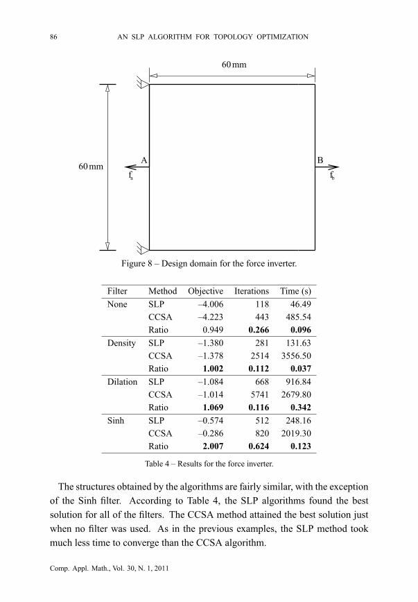
Our last problem is the design of a compliant mechanism known as forceinverter. The domain is shown in Figure 8. In this example, an input forcefa is applied to the center of the left side of the domain and the mechanismshould generate an output force fb on the right side of the structure. Note thatboth fa and fb are horizontal, but have opposite directions. For this problem,we also use e = 1 mm, σ = 0.3 and E = 210000 N/mm2. The volume islimited by 20% of the design domain, and the input and output forces aregiven by fa = fb = 1 N . The domain was discretized into 3600 squareelements with 1 mm2. The filter radius was set to 2.5.

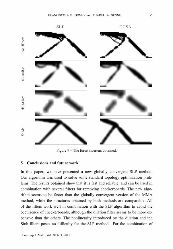
Figure 9 shows the mechanisms obtained. Again, only the upper half of thestructure is shown, due to its symmetry. Table 4 contains the numerical results.


“main” — 2011/2/5 — 12:32 — page 86 — #34


A

fb

B

60mm

fa60mm

Figure 8 – Design domain for the force inverter.


None SLP –4.006 118 46.49CCSA –4.223 443 485.54Ratio 0.949 0.266 0.096

Density SLP –1.380 281 131.63CCSA –1.378 2514 3556.50Ratio 1.002 0.112 0.037

Dilation SLP –1.084 668 916.84CCSA –1.014 5741 2679.80Ratio 1.069 0.116 0.342

Sinh SLP –0.574 512 248.16CCSA –0.286 820 2019.30Ratio 2.007 0.624 0.123

Table 4 – Results for the force inverter.

The structures obtained by the algorithms are fairly similar, with the exceptionof the Sinh filter. According to Table 4, the SLP algorithms found the bestsolution for all of the filters. The CCSA method attained the best solution justwhen no filter was used. As in the previous examples, the SLP method tookmuch less time to converge than the CCSA algorithm.


“main” — 2011/2/5 — 12:32 — page 87 — #35


SLP CCSAnofilter

density

dilation

Sinh

Figure 9 – The force inverters obtained.

5 Conclusions and future work

In this paper, we have presented a new globally convergent SLP method.Our algorithm was used to solve some standard topology optimization prob-lems. The results obtained show that it is fast and reliable, and can be used incombination with several filters for removing checkerboards. The new algo-rithm seems to be faster than the globally convergent version of the MMAmethod, while the structures obtained by both methods are comparable. Allof the filters work well in combination with the SLP algorithm to avoid theoccurrence of checkerboards, although the dilation filter seems to be more ex-pensive than the others. The nonlinearity introduced by the dilation and theSinh filters poses no difficulty for the SLP method. For the combination of


“main” — 2011/2/5 — 12:32 — page 88 — #36


filter and trust region radii tested, the Sinh filter presented the best formedstructures. Some of the filters allowed the formation of one node hinges. Theimplementation of hinge elimination strategies, following the suggestions ofSilva [18], is one possible extension of this work. We also plan to analyze thebehavior of the SLP algorithm in combination with other compliant mecha-nism formulations, such as those proposed by Pedersen et al. [15], Min andKim [13], and Luo et al. [12].

Acknowledgements. We would like to thank Prof. Svanberg for supplyingthe source code of his algorithm and Talita for revising the manuscript.

REFERENCES

[1] M.P. Bendsøe, Optimal shape design as a material distribution problem. Struct.Optim., 1 (1989), 193–202.

[2] M.P. Bendsøe and N. Kikuchi, Generating optimal topologies in structural designusing a homogenization method. Comput. Methods Appl. Mech. Eng., 71 (1988),197–224.

[3] T.E. Bruns and D.A. Tortorelli, An element removal and reintroduction strategy forthe topology optimization of structures and compliant mechanisms. Int. J. Numer.Methods Eng., 57 (2003), 1413–1430.

[4] T.E. Bruns, A reevaluation of the SIMP method with filtering and an alterna-tive formulation for solid-void topology optimization. Struct. Multidiscipl. Optim.,30 (2005), 428–436.

[5] R.H. Byrd, N.I.M Gould and J. Nocedal, An active-set algorithm for nonlinearprogramming using linear programming and equality constrained subproblems.Report OTC 2002/4, Optimization Technology Center, Northwestern University,Evanston, IL, USA, (2002).

[6] C.M. Chin and R. Fletcher, On the global convergence of an SLP-filter algorithmthat takes EQP steps. Math. Program., 96 (2003), 161–177.

[7] A.R. Díaz and O. Sigmund, Checkerboard patterns in layout optimization. Struct.and Multidiscipl. Optim., 10 (1995), 40–45.

[8] R. Fletcher and E. Sainz de la Maza, Nonlinear programming and nonsmoothoptimization by sucessive linear programming. Math. Program., 43 (1989), 235–256.


“main” — 2011/2/5 — 12:32 — page 89 — #37


[9] F.A.M. Gomes, M.C. Maciel and J.M. Martínez, Nonlinear programming algo-rithms using trust regions and augmented Lagrangians with nonmonotone penaltyparameters. Math. Program., 84 (1999), 161–200.

[10] N. Kikuchi, S. Nishiwaki, J.S.F. Ono and E.C.S. Silva, Design optimizationmethod for compliant mechanisms and material microstructure. Comput. MethodsAppl. Mech. Eng., 151 (1998), 401–417.

[11] C.R. Lima, Design of compliant mechanisms using the topology optimizationmethod (in portuguese). Dissertation, University of São Paulo, SP, Brazil, (2002).

[12] Z. Luo, L. Chen, J. Yang, Y. Zhang and K. Abdel-Malek, Compliant mechanismdesign using multi-objective topology optimization scheme of continuum struc-tures. Struct. Multidiscipl. Optim., 30 (2005), 142–154.

[13] S. Min and Y. Kim, Topology Optimization of Compliant Mechanism with Geo-metrical Advantage. JSME Int. J. Ser. C, 47(2) (2004), 610–615.

[14] S. Nishiwaki, M.I. Frecker, M. Seungjae and N. Kikuchi, Topology optimiza-tion of compliant mechanisms using the homogenization method. Int. J. Numer.Methods Eng., 42 (1998), 535–559.

[15] C.B.W. Pedersen, T. Buhl and O. Sigmund, Topology synthesis of large-displace-ment compliant mechanisms. Int. J. Num. Methods Eng., 50 (2001), 2683–2705.

[16] O. Sigmund, On the design of compliant mechanisms using topology optimization.Mech. Struct. Mach., 25 (1997), 493–524.

[17] O. Sigmund, Morphology-based black and white filters for topology optimization.Struct. Multidiscipl. Optim., 33(4-5) (2007), 401–424.

[18] M.C. Silva, Topology optimization to design hinge-free compliant mechanisms (inportuguese). Dissertation, University of São Paulo, SP, Brazil, (2007).

[19] K. Svanberg, The Method of Moving Asymptotes – A new method for structuraloptimization. Int. J. Numer. Methods Eng., 24 (1987), 359–373.

[20] K. Svanberg, A class of globally convergent optimization methods based on conser-vative convex separable approximations. SIAM J. Optim. 12(2) (2002), 555–573.

[21] Z. Zhang, N. Kim and L. Lasdon, An improved sucessive linear programming

algorithm. Manag. Science 31 (1985), 1312–1351.


an slp algorithm and its application to topology optimization*

Documents