A statistical assessment of seismic models of the U.S.continental crust using Bayesian inversionof ambient noise surface wavedispersion dataT. M. Olugboji1 , V. Lekic1 , and W. McDonough1

1Department of Geology, University of Maryland, College Park, Maryland, USA

Abstract We present a new approach for evaluating existing crustal models using ambient noise data setsand its associated uncertainties. We use a transdimensional hierarchical Bayesian inversion approach toinvert ambient noise surface wave phase dispersion maps for Love and Rayleigh waves using measurementsobtained from Ekström (2014). Spatiospectral analysis shows that our results are comparable to a linear leastsquares inverse approach (except at higher harmonic degrees), but the procedure has additional advantages:(1) it yields an autoadaptive parameterization that follows Earth structure without making restrictingassumptions onmodel resolution (regularization or damping) and data errors; (2) it can recover non-Gaussianphase velocity probability distributions while quantifying the sources of uncertainties in the datameasurements and modeling procedure; and (3) it enables statistical assessments of different crustal models(e.g., CRUST1.0, LITHO1.0, and NACr14) using variable resolution residual and standard deviation mapsestimated from the ensemble. These assessments show that in the stable old crust of the Archean, the misfitsare statistically negligible, requiring no significant update to crustal models from the ambient noise data set.In other regions of the U.S., significant updates to regionalization and crustal structure are expectedespecially in the shallow sedimentary basins and the tectonically active regions, where the differencesbetween model predictions and data are statistically significant.

1. Introduction

Seismological models of the crust are useful for making geological inference, for instance, when combinedwith other geophysical and geochemical constraints; they provide our best insight into the structure andcomposition of Earth’s continental crust [e.g., Christensen and Mooney, 1995; Hans Wedepohl, 1995; Huanget al., 2013; Rudnick and Gao, 2014]. The most widely used models are constrained by active source dataset of seismic reflection and refraction experiments and in a few cases receiver functions [e.g., Mooneyet al., 1998; Laske et al., 2012]. For this reason the models only sparsely sample the surface of the Earth andoften impose limiting assumptions by extrapolations based on tectonic regionalization. Additionally, thesemodels do not come with estimated uncertainties, making inferences hard to evaluate. We address thesetwo concerns for the conterminous United States where comprehensive seismic instrumentation is providedby EarthScope’s USArray [e.g., Long et al., 2014]. We use the extensive data sets of short-period, ambient noisephase velocity measurements for Love and Rayleigh surface waves.

Previous ambient noise seismic experiments included regional studies in both the western and eastern U.S.[Shapiro, 2005; Moschetti et al., 2007; Liang and Langston, 2008; Stachnik et al., 2008; Ekström et al., 2009] aswell as continent-wide studies [Bensen et al., 2008; Ekström, 2014]. Together, these data sets provide anunprecedented opportunity to constrain the elastic properties of the crust and upper mantle across theconterminous United States [e.g., Yang et al., 2008, 2011; Bensen et al., 2009; Moschetti et al., 2010a; Shenet al., 2013]. Despite the proliferation of measurements, neither regional models of the U.S. crust, e.g.,NACr14 [Tesauro et al., 2014] nor global models like Crust5.1 [Nataf and Ricard, 1996; Mooney et al., 1998],and its successors: Crust2.0 [Bassin et al., 2000], Crust1.0 [Laske et al., 2012], and LITHOS 1.0 [e.g., Pasyanoset al., 2014], incorporate ambient noise, passive source data sets into their inversions.

In this study, we use ambient noise data to evaluate crustal structure and its associated uncertainties. Indoing so, we apply transdimensional hierarchical Bayesian inversion (THBI) [e.g., Bodin and Sambridge,2009; Bodin et al., 2012b] to invert for a solution ensemble of phase velocity dispersion maps and the

OLUGBOJI ET AL. BAYESIAN EVALUATION OF U.S. CRUSTAL MODELS 1

PUBLICATIONSTectonics

RESEARCH ARTICLE10.1002/2017TC004468

Special Section:An appraisal of GlobalContinental Crust: Structureand Evolution

Key Points:• Transdimensional hierarchicalBayesian inversion of a phase velocitydispersion data set of ambient noisesurface waves for the continental U.S.

• Statistics derived from the MonteCarlo ensemble are compared to threepublished crustal models, showing afavorable comparison for LITHO1.0

• Misfits for the stable Archean crust arestatistically negligible, while shallowsedimentary basins and tectonicallyactive regions require updates

Supporting Information:• Supporting Information S1

Correspondence to:T. M. Olugboji,olugboji@umd.edu

Citation:Olugboji, T. M., V. Lekic, and W.McDonough (2017), A statistical assess-ment of seismic models of the U.S. con-tinental crust using Bayesian inversionof ambient noise surface wave disper-sion data, Tectonics, 36, doi:10.1002/2017TC004468.

Received 4 JAN 2017Accepted 5 JUN 2017Accepted article online 9 JUN 2017

©2017. American Geophysical Union.All Rights Reserved.

optimal parameterization for these maps. The Bayesian inverse approach estimates the model uncertain-ties from a large sample of the posterior distribution generated by a reversible jump Markov Chain MonteCarlo (rj-McMC) sampler. By extending the Bayesian approach to the problem of estimating the modelparameterization itself, we can invert for phase velocity maps without needing to make explicit, restrictingassumptions on the model resolution or regularization (smoothing or damping) as required by traditional,linear, least squares inverse approaches [e.g., Bensen et al., 2008; Ekström, 2014]. This allows us to recover,with greater confidence, fine-scale features in various sedimentary and rift basins, as well as across oro-genic zones within the crust of the U.S. Accurate reconstructions of the crustal velocities in these differenttectonic provinces are important for interpretation of the tectonic history and evolution of basins andorogens [e.g., Benoit et al., 2014; Pollitz and Mooney, 2014; Schmandt et al., 2015; Zhang et al., 2016;Hopper et al., 2017]. Additionally, they are important for making geophysical inferences about variationsof crustal composition across tectonic settings, with depth, and with age [e.g., Rudnick and Gao, 2014;Yuan, 2015].

Additionally, we estimate the aggregate uncertainty (“hierarchical” parameters) that arises from both thephase dispersion measurements and from errors introduced by simplifying assumption of great circle pathsin forward modeling [Young et al., 2013]. We quantify the similarities and differences betweenmaps obtainedby the standard, least squares versus the THBI inversions using a multiple taper, spherical Slepian approach[e.g., Simons et al., 2006]. Uncertainty estimates on phase velocity maps are needed to estimate the uncertain-ties of velocity profiles and, by extension, compositional inferences derived from such maps.

The solution ensemble provided by THBI allows us to quantify the uncertainty and trade-offs in the absolutephase velocity maps. The THBI approach to estimating phase dispersion maps is less biased by the artifacts ofinversion (i.e., regularization and linearization) and incorporates both observational (measurement) andmodeling uncertainty, constrained alongside the phase velocity uncertainties within the Bayesian inverseframework, differing from empirical approaches [e.g., Bensen et al., 2009; Shen et al., 2013; Ekström, 2014].

This statistical data set of phase dispersion maps can be used to propagate uncertainties into the next stageinversions for isotropic [e.g., Yang et al., 2008, 2011; Bensen et al., 2009;Moschetti et al., 2010a; Shen et al., 2013;Shen and Ritzwoller, 2016], and anisotropic [e.g., Moschetti et al., 2010b; Dalton and Gaherty, 2013; Lin andSchmandt, 2014] compressional and shear wave velocities in the U.S. continental crust. Moreover, we canaddress questions that a typical geoscientist might ask: “To what degree will this data set inform existing crus-tal models?” or “In which regions of data availability will new crustal models derived from this data set differfrom previous versions, within data uncertainty?”

We answer these questions by comparing the residuals derived from the THBI and those predicted by pre-viousmodels. We assess regions within the U.S. where existing crustal models fit the new data set and regionswhere significant updates are required, based on the current level of uncertainty (i.e., probability distribu-tions). We discuss how future geological and geophysical studies, which rely on existing crustal models,can assess the usefulness of these models, while highlighting which parts of the existing models will requiresignificant updates.

2. Phase Velocity Measurements and Uncertainty

We use the data set of interstation phase velocity measurements reported by Ekström [2014]. These measure-ments are made from ambient noise Love and Rayleigh waves at 11 discrete periods between 5 and 40 s andare obtained by an automated frequency domainmethod using spatial autocorrelation (SPAC) [e.g., Aki, 1957;Ekström et al., 2009; Prieto et al., 2009; Ekström, 2014; Menke and Jin, 2015]. In its implementation, originallydeveloped by Aki [1957] and extended by Ekström et al. [2009] and Ekström [2014], phase velocity dispersioncurves for a pair of stations are extracted by fitting the zero crossings of the real part of the cross-correlationspectra to the zeros of a Bessel function of the first kind. The cross-correlation spectra are stacked from a largedata set of 4 h long waveform records and are therefore resistant to strong earthquake signals. This studyrepresents the most comprehensive data set of ambient noise phase velocity measurements across thecontinental United States to date. Compared to the time domain cross-correlation method [e.g., Bensenet al., 2007], the SPAC method allows recovery of phase velocity measurements between closer station pairs[e.g., Tsai and Moschetti, 2010] (see also Ekström [2014] and Table 1).

Tectonics 10.1002/2017TC004468

OLUGBOJI ET AL. BAYESIAN EVALUATION OF U.S. CRUSTAL MODELS 2

In order to quantify reliably uncertainty in the phase dispersionmaps, which will be used to statistically assessthe predictive power of existing crustal models, we must estimate uncertainties associated with the under-lying dispersion measurements. One approach is to assign measurement uncertainties empirically by asses-sing their repeatability or formal uncertainty using a single-mode assumption or isotropic distribution ofnoise sources [e.g., Tsai and Moschetti, 2010; Ekström, 2014]. However, the relevant data uncertainties resultfrom a combination of measurement and modeling uncertainties, such as errors arising from the use of aray theoretical approximation to model the spatial pattern of wave sensitivity. Therefore, we opt to estimatethe aggregate data-related uncertainty explicitly, using a hierarchical Bayesian approach. We compare ourBayesian estimates of uncertainty to the empirical estimates of measurement uncertainty reported byEkström [2014].

We conduct a series of numerical experiments, in which data uncertainty is allowed to vary with path length,to assess the relative contribution of measurement versus modeling uncertainty at each period. By estimatingthe level of uncertainty in the Bayesian inversion (a more conservative estimate, in most cases) we reduce therisk of mapping measurement errors into spurious features in the recovered phase velocity maps, especiallyfor shorter periods where measurement uncertainties are large and strongly path length dependent (seesection 4.3 for more details).

3. Transdimensional Inversion

The transdimensional hierarchical Bayesian inverse (THBI) method we employ is similar to that describedby previous authors [e.g., Bodin and Sambridge, 2009; Bodin et al., 2012b; Young et al., 2013; Saygin et al.,2016]. The THBI approach generates an ensemble of models that fit the data, unlike the classic leastsquares approach that produces a single optimal model using an a priori fixed parameterization. In the

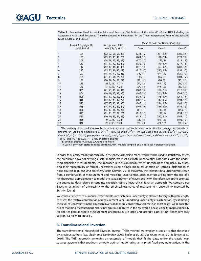
Table 1. Parameters Used to set the Prior and Proposal Distributions of the rj-McMC of the THBI Including theAcceptance Ratios and Recovered Transdimensional, n, Parameters for the Three Independent Runs of the rj-McMC(Case 1, Case 2, and Case 3)a

Love (L) Rayleigh (R)and Period

Acceptance Ratiosin % (bB, D, M, C, N)

Mean of Posterior Distribution (n, σ)

Case 1 Case 2 Case 3c

1 L05 (22, 22, 50, 58, 33) (234, 4.2) (231, 4.2) (386, 3.5)2 L06 (19, 19, 43, 49, 28) (204, 3.1) (190, 3.4) (373, 2.6)3 L08 (18, 18, 43, 43, 27) (170, 2.2) (175, 2) (313, 1.8)4 L10 (17, 17, 42, 40, 27) (132, 1.9) (140, 1.7) (217, 1.6)5 L12 (17, 17, 46, 41, 30) (116, 1.8) (124, 1.7) (200, 1.6)6 L15 (15, 15, 40, 33, 27) (116, 1.5) (115, 1.5) (193, 1.5)7 L20 (14, 14, 41, 30, 28) (96, 1.1) (97, 1.1) (120, 1.2)8 L25 (11, 11, 36, 24, 25) (85, 1) (86, 1) (104, 1.2)9 L30 (10, 10, 34, 21, 22) (92, 1.2) (86, 1) (93, 1.2)10 L35 (9, 9, 36, 19, 21) (71, 1.2) (65, 1.1) (66, 1.3)11 L40 (7, 7, 38, 17, 20) (54, 1.4) (49, 1.3) (49, 1.5)12 R05 (21, 21, 49, 52, 31) (183, 3.2) (196, 3.1) (316, 2.7)13 R06 (19, 19, 47, 47, 30) (146, 2.6) (161, 2.5) (304, 2.1)14 R08 (17, 17, 42, 39, 27) (134, 1.9) (145, 1.7) (251, 1.6)15 R10 (17, 17, 43, 37, 27) (108, 1.7) (117, 1.5) (194, 1.5)16 R12 (17, 17, 45, 37, 30) (107, 1.6) (114, 1.6) (183, 1.5)17 R15 (14, 14, 37, 29, 27) (105, 1.4) (116, 1.3) (183, 1.3)18 R20 (13, 13, 38, 26, 28) (111, 1) (113, 1) (159, 1)19 R25 (11, 11, 33, 22, 25) (115, 1.1) (117, 1) (154, 1.1)20 R30 (10, 10, 33, 21, 25) (113, 1.1) (113, 1.1) (144, 1.1)21 R35 (9, 9, 34, 19, 24) (95, 1.3) (93, 1.1) (108, 1.3)22 R40 (9, 9, 36, 18, 23) (81, 1.3) (79, 1.3) (86, 1.5)

aThe similarity of the n value across the three independent cases is a heuristic justification for convergence. Bounds ofuniform PDF used in the model priors. (σL, σH) = (0.1, 10) and (vL, vH) = (1.0, 6.0). Case 1 and Case 2: (σL, σH) = (50–600),Case 3: (σL, σH) = (50–200), proposal variances:Ωσ = 0.5,Ωn = 1,Ωv = 1.0. Case 1, Case 2, and Case 3: NS = 3 × 106, 1 × 107,1 × 107 and NR = 1000, NC = 10 (no. of parallel chains).

bB, Birth; D, Death; M, Move; C, Change; N, noise.cIn Case 3, the chain starts from the Ekström [2014] models sampled on an 1848 cell Voronoi tesellation.

Tectonics 10.1002/2017TC004468

OLUGBOJI ET AL. BAYESIAN EVALUATION OF U.S. CRUSTAL MODELS 3

Bayesian framework, a Monte Carlo sampler generates posterior distributions on model parameters fromwhich an ensemble average and uncertainty and trade-off estimates are made. The term “transdimen-sional” implies that in addition to the typical model parameters (e.g., phase velocity values within a spatialdomain), the model dimension (number of parameters required to represent phase velocity variations) isalso constrained during the inversion [e.g., Sambridge et al., 2006, 2012]. Voronoi tessellation is a discreteparameterization of the two-dimensional continuous seismic phase velocity field that captures velocityvariations at irregular spatial scales [e.g., Sambridge et al., 1995]. The tessellation partitions the plane inton nonoverlapping regions, using a nearest neighbor interpolation described by 3n parameters: a set of nvelocity values (vi , . . , vn) at nodal points described with 2n (longitude and latitude) location parameters(see Figure 1). It is this number n and the associated node coordinates that we wish to determine in thetransdimensional step of the THBI method.

In the “hierarchical-Bayes” step, at each period, we include an extra parameter (σ: the uncertainty (noise) scal-ing—equation (2)) to be constrained by the data during the Bayesian inversion. This parameter is considereda “hierarchical” parameter because it sits at a higher level in the inversion process. It is estimated before cal-culating the model fit of predicted to observed data for each velocity update step (i.e., lower level modelparameters) that contributes to the final two-dimensional phase velocity map [e.g., Malinverno and Briggs,2004; Malinverno and Parker, 2006; Bodin et al., 2012b]. Contributions of measurement and modeling uncer-tainties are quantified by rerunning the chain for three different subsets of the data, assigning different σvalues for the different subsets: short, medium, and long path lengths (see Table 2 for cutoff limits in km).This analysis shows that the hierarchical parameter is dominated by measurement uncertainty, which isstrongly path dependent (see section 4.3 for details).

On the whole, the Bayesian approach describes a posterior probability density function, p(m| d), on threeclasses of model parameters, m= {σ,n, and vi} (i.e., noise σ, model dimension n, and phase velocity valuesat the nodal points, vi) given as follows:

p mjdð Þ∝p djmð Þp mð Þ; (1)

where p(d|m) is the likelihood function, which describes the probability of the predicted model given theobserved data, d (and includes the hierarchical noise parameter σ):

p djmð Þ∝ exp� g mð Þ � dk k22σ2

( )(2)

In our forward calculation of the predicted travel times, g(m), we approximate the geographical sensitivity ofwaves between station pairs by great circles, rather than using finite frequency kernels. A uniform probabilitydensity function, p(m), describes our prior information on the model parameters, and in the case of the phasevelocity is represented by a range that encompasses all possible values for each period range (see Table 1),while for the noise and model dimension parameters, we use a range wide enough to include the most likelyvalue, after an initial trial and error process. We sample the posterior probability distribution using a variationof the Metropolis Hastings method known as the reversible jump Markov chain Monte Carlo (rj-McMC) algo-rithm that explores a probability space with varying dimensions [e.g., Green, 1995, 2003]. There are five kindsof proposal steps in the rj-McMC, with each proposal step selected with equal probability (see overview inFigure 1): the first three steps involve the proposal of a newmodelmp by a “transdimensional” transformationstep where the number, n, or configuration of the cells are changed (via (1) birth, (2) death, or (3) move); andthe last two steps involve (4) a fixed-dimension transformation step (changing a cell velocity value, vi) or (5) ahierarchical step (changing the noise scaling parameter, λj in σ = λjσ).

Eachnewmodel in theproposal step,mp, is sampled fromaGaussiandistribution,q (mp|mj),which requires theperturbation of the precedingmodel,mj, using proposal variances,Ωm(one for each model type:Ωσ ,Ωn ,Ωv):

mp ¼ mj þ uΩm; (3)

where u is drawn from a Gaussian distribution N (0,1). With the prior distribution and the proposal variationsset, the evolution of the chain is then governed by the acceptance probability, A (mp|mj), which determineswhether or not the current model,mj, will be retained or replaced by the proposed modelmp. This happens ifU ≤A (mp| mj), where U is a random number generated from a uniform distribution between 0 and 1 (for a

Tectonics 10.1002/2017TC004468

OLUGBOJI ET AL. BAYESIAN EVALUATION OF U.S. CRUSTAL MODELS 4

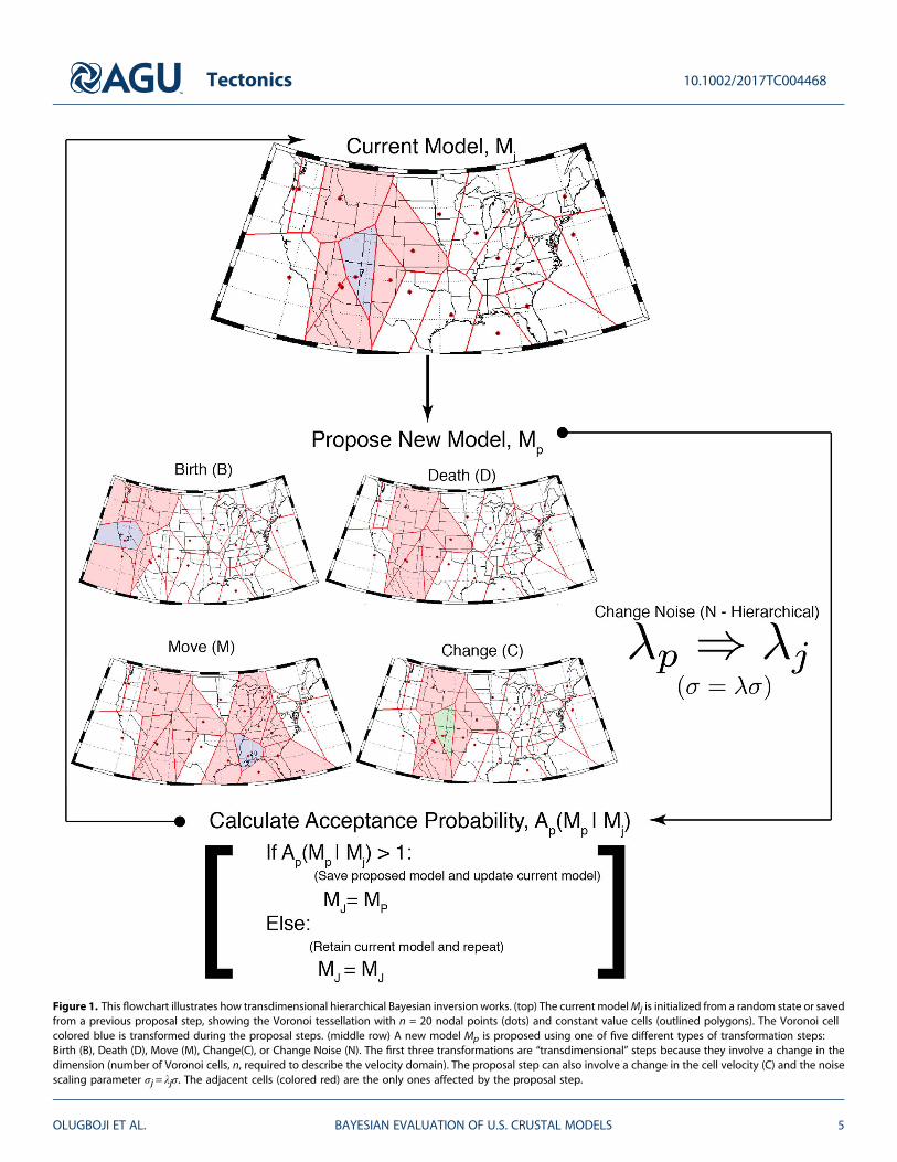
Figure 1. This flowchart illustrates how transdimensional hierarchical Bayesian inversion works. (top) The current modelMj is initialized from a random state or savedfrom a previous proposal step, showing the Voronoi tessellation with n = 20 nodal points (dots) and constant value cells (outlined polygons). The Voronoi cellcolored blue is transformed during the proposal steps. (middle row) A new model Mp is proposed using one of five different types of transformation steps:Birth (B), Death (D), Move (M), Change(C), or Change Noise (N). The first three transformations are “transdimensional” steps because they involve a change in thedimension (number of Voronoi cells, n, required to describe the velocity domain). The proposal step can also involve a change in the cell velocity (C) and the noisescaling parameter σj = λjσ. The adjacent cells (colored red) are the only ones affected by the proposal step.

Tectonics 10.1002/2017TC004468

OLUGBOJI ET AL. BAYESIAN EVALUATION OF U.S. CRUSTAL MODELS 5

complete discussion of how the acceptance probability, proposal distributions, and prior distributions aredefined see Bodin et al. [2012a, 2012b]). The range of the prior distribution and the proposal variances arethe only free parameters to be selected, and they are chosen to balance the convergence rate with efficientsampling of the model space (Table 1).

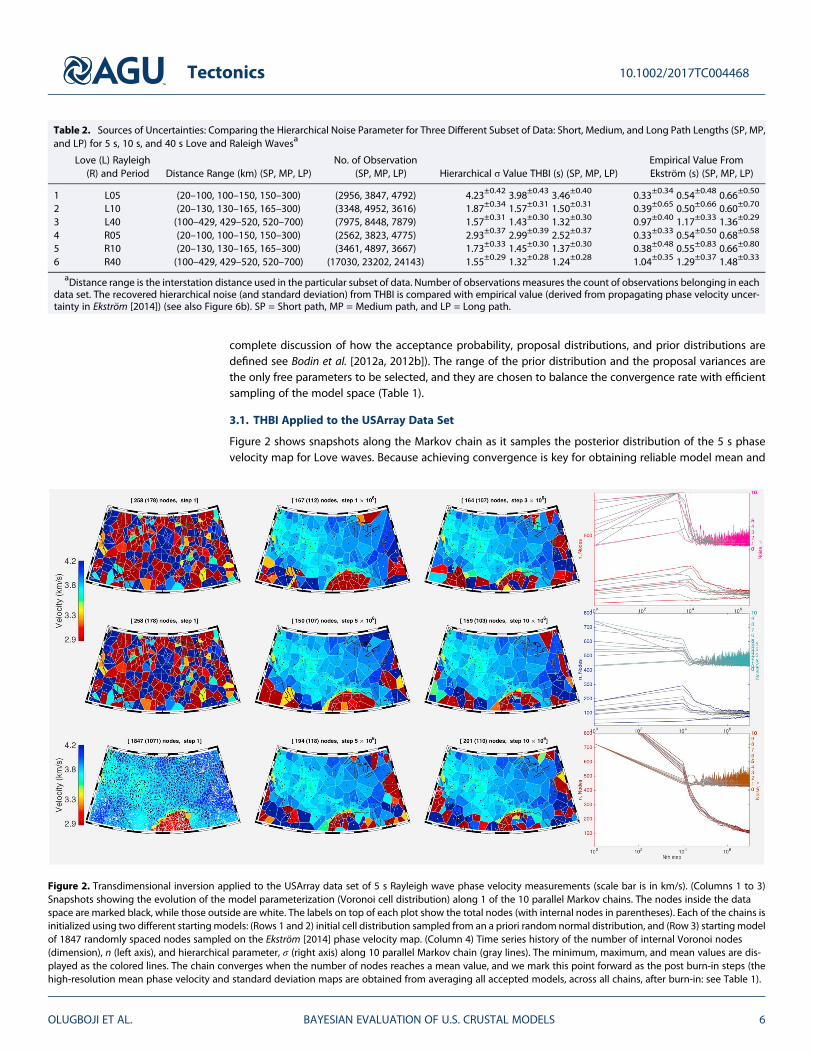
3.1. THBI Applied to the USArray Data Set

Figure 2 shows snapshots along the Markov chain as it samples the posterior distribution of the 5 s phasevelocity map for Love waves. Because achieving convergence is key for obtaining reliable model mean and

Table 2. Sources of Uncertainties: Comparing the Hierarchical Noise Parameter for Three Different Subset of Data: Short, Medium, and Long Path Lengths (SP, MP,and LP) for 5 s, 10 s, and 40 s Love and Raleigh Wavesa

Love (L) Rayleigh(R) and Period Distance Range (km) (SP, MP, LP)

No. of Observation(SP, MP, LP) Hierarchical σ Value THBI (s) (SP, MP, LP)

Empirical Value FromEkström (s) (SP, MP, LP)

1 L05 (20–100, 100–150, 150–300) (2956, 3847, 4792) 4.23±0.42 3.98±0.43 3.46±0.40 0.33±0.34 0.54±0.48 0.66±0.50

2 L10 (20–130, 130–165, 165–300) (3348, 4952, 3616) 1.87±0.34 1.57±0.31 1.50±0.31 0.39±0.65 0.50±0.66 0.60±0.70

3 L40 (100–429, 429–520, 520–700) (7975, 8448, 7879) 1.57±0.31 1.43±0.30 1.32±0.30 0.97±0.40 1.17±0.33 1.36±0.29

4 R05 (20–100, 100–150, 150–300) (2562, 3823, 4775) 2.93±0.37 2.99±0.39 2.52±0.37 0.33±0.33 0.54±0.50 0.68±0.58

5 R10 (20–130, 130–165, 165–300) (3461, 4897, 3667) 1.73±0.33 1.45±0.30 1.37±0.30 0.38±0.48 0.55±0.83 0.66±0.80

6 R40 (100–429, 429–520, 520–700) (17030, 23202, 24143) 1.55±0.29 1.32±0.28 1.24±0.28 1.04±0.35 1.29±0.37 1.48±0.33

aDistance range is the interstation distance used in the particular subset of data. Number of observations measures the count of observations belonging in eachdata set. The recovered hierarchical noise (and standard deviation) from THBI is compared with empirical value (derived from propagating phase velocity uncer-tainty in Ekström [2014]) (see also Figure 6b). SP = Short path, MP = Medium path, and LP = Long path.

Figure 2. Transdimensional inversion applied to the USArray data set of 5 s Rayleigh wave phase velocity measurements (scale bar is in km/s). (Columns 1 to 3)Snapshots showing the evolution of the model parameterization (Voronoi cell distribution) along 1 of the 10 parallel Markov chains. The nodes inside the dataspace are marked black, while those outside are white. The labels on top of each plot show the total nodes (with internal nodes in parentheses). Each of the chains isinitialized using two different startingmodels: (Rows 1 and 2) initial cell distribution sampled from an a priori random normal distribution, and (Row 3) startingmodelof 1847 randomly spaced nodes sampled on the Ekström [2014] phase velocity map. (Column 4) Time series history of the number of internal Voronoi nodes(dimension), n (left axis), and hierarchical parameter, σ (right axis) along 10 parallel Markov chain (gray lines). The minimum, maximum, and mean values are dis-played as the colored lines. The chain converges when the number of nodes reaches a mean value, and we mark this point forward as the post burn-in steps (thehigh-resolution mean phase velocity and standard deviation maps are obtained from averaging all accepted models, across all chains, after burn-in: see Table 1).

Tectonics 10.1002/2017TC004468

OLUGBOJI ET AL. BAYESIAN EVALUATION OF U.S. CRUSTAL MODELS 6

uncertainty estimates, we use three different modeling approaches: running either (1) 10 parallel chains runfor 3 million steps initialized from a random start state drawn from a uniform prior distribution with 379Voronoi nodes, (2) the same procedures as Case 1 but using 10 million steps in each chain, and (3) 10 parallelchains run for 10 million steps but initialized from a high-density (1847 node) discretization of the mean mapreported by Ekström [2014]. In all cases, the chain takes only ~100,000 steps to converge to an optimal state(through birth, death, move, and cell change steps). Somewhat surprisingly, the nodal density, misfit, andother key inversion parameters are similar across solutions, independent of the starting state (see Figure 2and Table 1), suggesting that global convergence is achieved and that the posterior ensemble is representa-tive p(m|d). The same solution is recovered for modeling approach 3, despite using a high-density startingmodel, demonstrating that the THBI always produces a parsimonious solution; i.e., it looks for model to fitthe data using the simplest parameterization possible. The time to reach this optimal state is called theburn-in period, and only models that are generated after this period (post burn-in) are used to build the pos-terior distribution and derive the final ensemble average of mean, standard deviation, and trade-off maps.During the sampling, only model updates that change the data misfit are accepted as valid proposal steps.This ensures that regions with no data are locked in (i.e., white dots in Figure 2).

3.2. Mean and Standard Deviation Phase Velocity Maps

In our construction of the mean and standard deviation maps, we sparsely resample the ensemble to ensurethat the aggregated models are not correlated. First, we construct high-resolution mean phase velocity mapsby interpolating the Voronoi tessellation on a regular 600 × 600 grid, using only the post burn-in samplesfrom the multiple chains. The total number of samples used in the averaging scheme, NT, is a function ofthe total number of steps per chain, NS, the number of independent Markov chains, NC, the number ofburn-in steps, NB, and the resampling rate NR:

NT ¼ NS�NB

NR

� �� NC

The final ensemble is resampled at every thousandth step (NR=1000) to ensure that models used in the finalaverage are not correlated. For example, in the longest run of the 5 s Love wave, the total number of samplesused to produce the mean phase velocity map is NT~104 (Ns=107, NR= 103,NB= 106 , and NC=101)(Figure 3). In the run for Case 3, the convergence is faster (smaller burn-in steps compared to Case 1 andCase 2), since the starting model is already close to the true solution. We report the number of burn-in steps,the postconvergence nodal density, and the postconvergence hierarchical noise parameter for the otherLove and Rayleigh maps in Table 1.

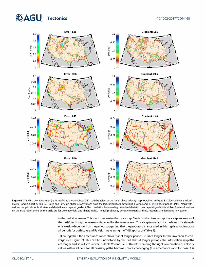
Next, we use the mean phase velocity maps to derive the standard deviation maps (using similar post burn-inensemble and resampling strategy). Areas in thesemaps with low standard deviation showwhich parts of theaverage models in Figure 3 are well constrained. Large uncertainties in regions with no data are trivial toexplain; however, where data exist, there are some regions of high standard deviation. The outline of thesehigh standard deviation regions is similar to features in the mean models associated with velocity gradients.We therefore compute a spatial gradient of the velocity fields for comparison with the standard deviationmaps. A high correlation between these two maps confirms our intuition that high gradients contribute tohigh uncertainty (Column 2 versus Column 1 in Figure 4).

3.3. Monte Carlo Search Efficiency

As described above, during the rj-McMC sampling, each of the five steps in the THBI has an equal like-lihood of being selected (see Figure 1), and for each model proposed, the ratio of acceptance is deter-mined by the prescribed proposal variances, Ωm, (e.g., equation (3) in section 3). The search efficiencycan be quantified by the acceptance ratios (ratio of number of proposed models to accepted models,see Table 1).

We observe that for both the Love and Rayleigh wave inversions, the move or change steps have the highestacceptance ratios (as large as 50%), followed by the hierarchical step (~30%) and the birth/death step(~20%). Compared to the change step, themove step is preferred, especially for periods>10 s. This is becauseit is easier to improve the data fit using a move step compared to a change step. At longer periods, the accep-tance ratio decreases, suggesting that for the chosen proposal variances, it takes longer to find good models

Tectonics 10.1002/2017TC004468

OLUGBOJI ET AL. BAYESIAN EVALUATION OF U.S. CRUSTAL MODELS 7

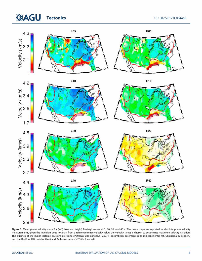
Figure 3. Mean phase velocity maps for (left) Love and (right) Rayleigh waves at 5, 10, 20, and 40 s. The mean maps are reported in absolute phase velocitymeasurements, given the inversion does not start from a reference mean velocity value; the velocity range is chosen to accentuate maximum velocity variation.The outlines of the major tectonic divisions are from Whitmeyer and Karlstrom [2007]: Precambrian basement (red), midcontinental rift, Oklahoma aulacogen,and the Reelfoot Rift (solid outline) and Archean cratons >2.5 Ga (dashed).

Tectonics 10.1002/2017TC004468

OLUGBOJI ET AL. BAYESIAN EVALUATION OF U.S. CRUSTAL MODELS 8

as theperiod increases. This is not the case for themove step. Similar to the change step, the acceptance ratio ofthebirth/death stepdecreaseswithperiod for the same reason. The acceptance ratio for thehierarchical step isonlyweakly dependent on the period, suggesting that the proposal variance used in this step is suitable acrossall periods for both Love and Rayleigh wave using the THBI approach (Table 1).

Taken together, the acceptance ratios show that at longer periods, it takes longer for the inversion to con-verge (see Figure 2). This can be understood by the fact that at longer periods, the interstation raypathsare longer and so will cross over multiple Voronoi cells. Therefore, finding the right combination of velocityvalues within all cells for all crossing paths becomes more challenging (the acceptance ratio for Case 3 is

Figure 4. Standard deviationmaps (at 3σ level) and the associated 2-D spatial gradient of themean phase velocity maps obtained in Figure 3 (color scale bar is in km/s).(Rows 1 and 2) Short-period (5 s) Love and Rayleigh phase velocity maps have the largest standard deviations. (Rows 3 and 4). The longest periods (40 s) maps withreduced amplitude for both standard deviation and spatial gradient. The correlation between high standard deviations and spatial gradient is visible. The two locationson the map represented by the circle are for Colorado (left) and Illinois (right). The full probability density functions at these locations are described in Figure 6.

Tectonics 10.1002/2017TC004468

OLUGBOJI ET AL. BAYESIAN EVALUATION OF U.S. CRUSTAL MODELS 9

larger since the chain starts from an optimal model; see supporting information Table S1). Following therecommendation of Ray et al. [2013], we increase the acceptance ratio of the birth/death step by decreasingthe proposal step size, Ωv, from 1.0 to 0.1; we also reduce the prior range, (vL and vH), (from 1.0–6.0 km/s to2.0–4.5 km/s). These new parameters improve the acceptance ratio for the longer period maps.

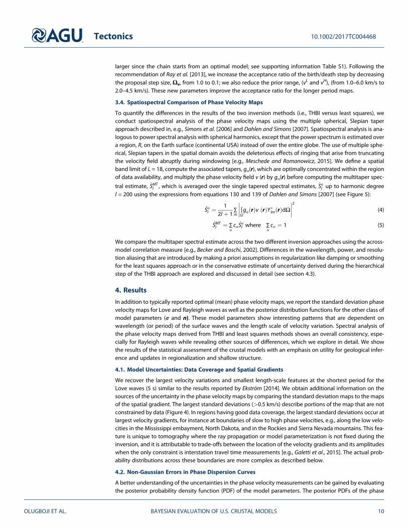
3.4. Spatiospectral Comparison of Phase Velocity Maps

To quantify the differences in the results of the two inversion methods (i.e., THBI versus least squares), weconduct spatiospectral analysis of the phase velocity maps using the multiple spherical, Slepian taperapproach described in, e.g., Simons et al. [2006] and Dahlen and Simons [2007]. Spatiospectral analysis is ana-logous to power spectral analysis with spherical harmonics, except that the power spectrum is estimated overa region, R, on the Earth surface (continental USA) instead of over the entire globe. The use of multiple sphe-rical, Slepian tapers in the spatial domain avoids the deleterious effects of ringing that arise from truncatingthe velocity field abruptly during windowing [e.g., Meschede and Romanowicz, 2015]. We define a spatialband limit of L = 18, compute the associated tapers, gα(r), which are optimally concentrated within the regionof data availability, and multiply the phase velocity field v (r) by gα(r) before computing the multitaper spec-

tral estimate, SMTl , which is averaged over the single tapered spectral estimates, Sαl up to harmonic degree

l = 200 using the expressions from equations 130 and 139 of Dahlen and Simons [2007] (see Figure 5):

Sαl ¼1

2l þ 1∑m

∫Ωgα rð Þv rð ÞY�

lm rð ÞdΩ����

����2

(4)

SMTl ¼ ∑

αcαS

αl where ∑

αcα ¼ 1 (5)

We compare the multitaper spectral estimate across the two different inversion approaches using the across-model correlation measure [e.g., Becker and Boschi, 2002]. Differences in the wavelength, power, and resolu-tion aliasing that are introduced by making a priori assumptions in regularization like damping or smoothingfor the least squares approach or in the conservative estimate of uncertainty derived during the hierarchicalstep of the THBI approach are explored and discussed in detail (see section 4.3).

4. Results

In addition to typically reported optimal (mean) phase velocity maps, we report the standard deviation phasevelocity maps for Love and Rayleigh waves as well as the posterior distribution functions for the other class ofmodel parameters (σ and n). These model parameters show interesting patterns that are dependent onwavelength (or period) of the surface waves and the length scale of velocity variation. Spectral analysis ofthe phase velocity maps derived from THBI and least squares methods shows an overall consistency, espe-cially for Rayleigh waves while revealing other sources of differences, which we explore in detail. We showthe results of the statistical assessment of the crustal models with an emphasis on utility for geological infer-ence and updates in regionalization and shallow structure.

4.1. Model Uncertainties: Data Coverage and Spatial Gradients

We recover the largest velocity variations and smallest length-scale features at the shortest period for theLove waves (5 s) similar to the results reported by Ekström [2014]. We obtain additional information on thesources of the uncertainty in the phase velocity maps by comparing the standard deviationmaps to themapsof the spatial gradient. The largest standard deviations (>0.5 km/s) describe portions of the map that are notconstrained by data (Figure 4). In regions having good data coverage, the largest standard deviations occur atlargest velocity gradients, for instance at boundaries of slow to high phase velocities, e.g., along the low velo-cities in the Mississippi embayment, North Dakota, and in the Rockies and Sierra Nevada mountains. This fea-ture is unique to tomography where the ray propagation or model parameterization is not fixed during theinversion, and it is attributable to trade-offs between the location of the velocity gradients and its amplitudeswhen the only constraint is interstation travel time measurements [e.g., Galetti et al., 2015]. The actual prob-ability distributions across these boundaries are more complex as described below.

4.2. Non-Gaussian Errors in Phase Dispersion Curves

A better understanding of the uncertainties in the phase velocity measurements can be gained by evaluatingthe posterior probability density function (PDF) of the model parameters. The posterior PDFs of the phase

Tectonics 10.1002/2017TC004468

OLUGBOJI ET AL. BAYESIAN EVALUATION OF U.S. CRUSTAL MODELS 10

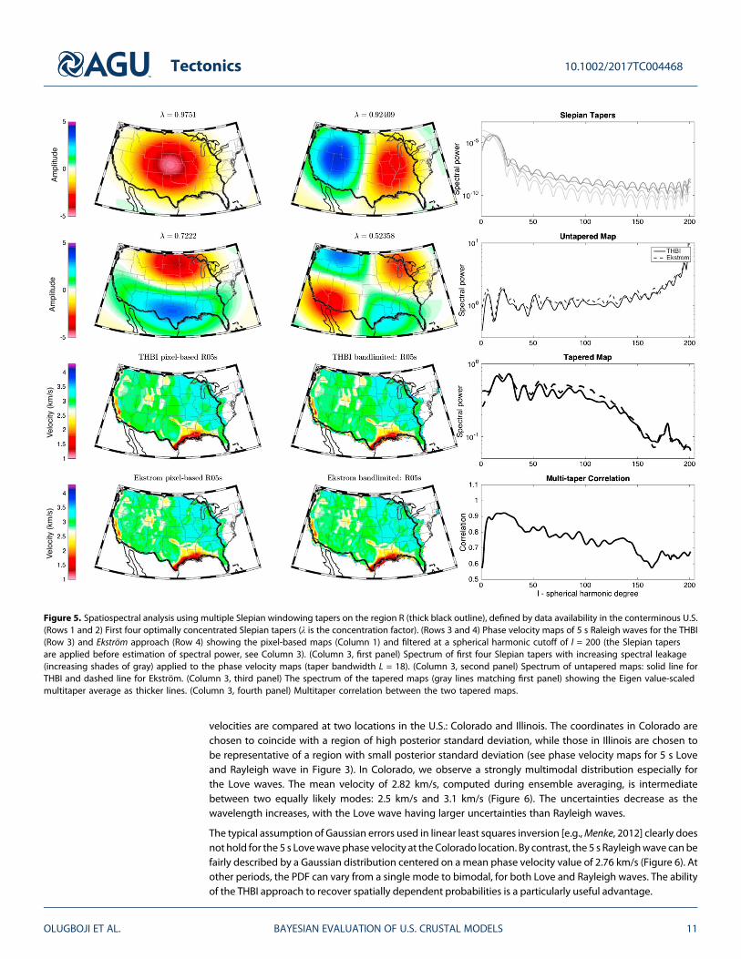
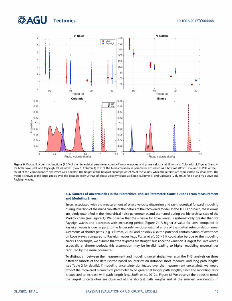
velocities are compared at two locations in the U.S.: Colorado and Illinois. The coordinates in Colorado arechosen to coincide with a region of high posterior standard deviation, while those in Illinois are chosen tobe representative of a region with small posterior standard deviation (see phase velocity maps for 5 s Loveand Rayleigh wave in Figure 3). In Colorado, we observe a strongly multimodal distribution especially forthe Love waves. The mean velocity of 2.82 km/s, computed during ensemble averaging, is intermediatebetween two equally likely modes: 2.5 km/s and 3.1 km/s (Figure 6). The uncertainties decrease as thewavelength increases, with the Love wave having larger uncertainties than Rayleigh waves.

The typical assumption of Gaussian errors used in linear least squares inversion [e.g.,Menke, 2012] clearly doesnot hold for the 5 s Lovewavephase velocity at the Colorado location. By contrast, the 5 s Rayleighwave canbefairly described by a Gaussian distribution centered on a mean phase velocity value of 2.76 km/s (Figure 6). Atother periods, the PDF can vary from a single mode to bimodal, for both Love and Rayleigh waves. The abilityof the THBI approach to recover spatially dependent probabilities is a particularly useful advantage.

Figure 5. Spatiospectral analysis using multiple Slepian windowing tapers on the region R (thick black outline), defined by data availability in the conterminous U.S.(Rows 1 and 2) First four optimally concentrated Slepian tapers (λ is the concentration factor). (Rows 3 and 4) Phase velocity maps of 5 s Raleigh waves for the THBI(Row 3) and Ekström approach (Row 4) showing the pixel-based maps (Column 1) and filtered at a spherical harmonic cutoff of l = 200 (the Slepian tapersare applied before estimation of spectral power, see Column 3). (Column 3, first panel) Spectrum of first four Slepian tapers with increasing spectral leakage(increasing shades of gray) applied to the phase velocity maps (taper bandwidth L = 18). (Column 3, second panel) Spectrum of untapered maps: solid line forTHBI and dashed line for Ekström. (Column 3, third panel) The spectrum of the tapered maps (gray lines matching first panel) showing the Eigen value-scaledmultitaper average as thicker lines. (Column 3, fourth panel) Multitaper correlation between the two tapered maps.

Tectonics 10.1002/2017TC004468

OLUGBOJI ET AL. BAYESIAN EVALUATION OF U.S. CRUSTAL MODELS 11

4.3. Sources of Uncertainties in the Hierarchical (Noise) Parameter: Contributions From Measurementand Modeling Errors

Errors associated with the measurement of phase velocity dispersion and ray-theoretical forward modelingduring inversion of the maps can affect the details of the recovered model. In the THBI approach, these errorsare jointly quantified in the hierarchical noise parameter, σ, and estimated during the hierarchical step of theMarkov chain (see Figure 1). We observe that the σ value for Love waves is systematically greater than forRayleigh waves and decreases with increasing period (Figure 7). A higher σ value for Love compared toRayleigh waves is due, in part, to the larger relative observational errors of the spatial autocorrelation mea-surements at shorter paths [e.g., Ekström, 2014], and possibly also the potential contamination of overtoneson Love waves compared to Rayleigh waves [e.g., Foster et al., 2014]. It could also be due to the modelingerrors. For example, we assume that the raypaths are straight, but since the variation is largest for Love waves,especially at shorter periods, this assumption may be invalid, leading to higher modeling uncertaintiescaptured by the noise parameter.

To distinguish between the measurement and modeling uncertainties, we rerun the THBI analysis on threedifferent subsets of the data (sorted based on interstation distance: short, medium, and long path lengths(see Table 2 for details). If modeling uncertainty dominated over the measurement uncertainty, we wouldexpect the recovered hierarchical parameter to be greater at longer path lengths, since the modeling erroris expected to increase with path length [e.g., Bodin et al., 2012b, Figure 8]. We observe the opposite trend:the largest uncertainties are observed at the shortest path lengths and at the smallest wavelength, in

Figure 6. Probability density functions (PDF) of the hierarchical parameter, count of Voronoi nodes, and phase velocity (at Illinois and Colorado: cf. Figures 3 and 4)for both Love (red) and Rayleigh (blue) waves. (Row 1, Column 1) PDF of the hierarchical noise parameter expressed as a boxplot. (Row 1, Column 2) PDF of thecount of the Voronoi nodes expressed as a boxplot. The height of the boxplot encompasses 99% of the values, while the outliers are represented by small dots. Themean is shown as the large circles over the boxplot. (Row 2) PDF of phase velocity values at Illinois (Column 1) and Colorado (Column 2) for 5 s and 40 s Love andRayleigh waves.

Tectonics 10.1002/2017TC004468

OLUGBOJI ET AL. BAYESIAN EVALUATION OF U.S. CRUSTAL MODELS 12

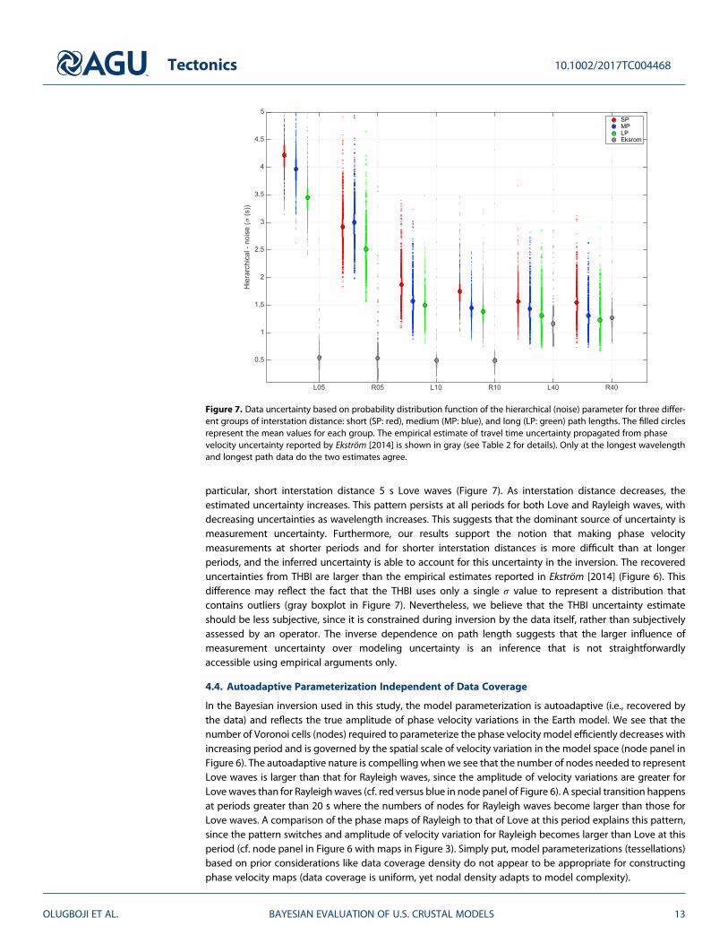
particular, short interstation distance 5 s Love waves (Figure 7). As interstation distance decreases, theestimated uncertainty increases. This pattern persists at all periods for both Love and Rayleigh waves, withdecreasing uncertainties as wavelength increases. This suggests that the dominant source of uncertainty ismeasurement uncertainty. Furthermore, our results support the notion that making phase velocitymeasurements at shorter periods and for shorter interstation distances is more difficult than at longerperiods, and the inferred uncertainty is able to account for this uncertainty in the inversion. The recovereduncertainties from THBI are larger than the empirical estimates reported in Ekström [2014] (Figure 6). Thisdifference may reflect the fact that the THBI uses only a single σ value to represent a distribution thatcontains outliers (gray boxplot in Figure 7). Nevertheless, we believe that the THBI uncertainty estimateshould be less subjective, since it is constrained during inversion by the data itself, rather than subjectivelyassessed by an operator. The inverse dependence on path length suggests that the larger influence ofmeasurement uncertainty over modeling uncertainty is an inference that is not straightforwardlyaccessible using empirical arguments only.

4.4. Autoadaptive Parameterization Independent of Data Coverage

In the Bayesian inversion used in this study, the model parameterization is autoadaptive (i.e., recovered bythe data) and reflects the true amplitude of phase velocity variations in the Earth model. We see that thenumber of Voronoi cells (nodes) required to parameterize the phase velocity model efficiently decreases withincreasing period and is governed by the spatial scale of velocity variation in the model space (node panel inFigure 6). The autoadaptive nature is compelling when we see that the number of nodes needed to representLove waves is larger than that for Rayleigh waves, since the amplitude of velocity variations are greater forLove waves than for Rayleighwaves (cf. red versus blue in node panel of Figure 6). A special transition happensat periods greater than 20 s where the numbers of nodes for Rayleigh waves become larger than those forLove waves. A comparison of the phase maps of Rayleigh to that of Love at this period explains this pattern,since the pattern switches and amplitude of velocity variation for Rayleigh becomes larger than Love at thisperiod (cf. node panel in Figure 6 with maps in Figure 3). Simply put, model parameterizations (tessellations)based on prior considerations like data coverage density do not appear to be appropriate for constructingphase velocity maps (data coverage is uniform, yet nodal density adapts to model complexity).

Figure 7. Data uncertainty based on probability distribution function of the hierarchical (noise) parameter for three differ-ent groups of interstation distance: short (SP: red), medium (MP: blue), and long (LP: green) path lengths. The filled circlesrepresent the mean values for each group. The empirical estimate of travel time uncertainty propagated from phasevelocity uncertainty reported by Ekström [2014] is shown in gray (see Table 2 for details). Only at the longest wavelengthand longest path data do the two estimates agree.

Tectonics 10.1002/2017TC004468

OLUGBOJI ET AL. BAYESIAN EVALUATION OF U.S. CRUSTAL MODELS 13

4.5. Comparison to Least Squares Inversion

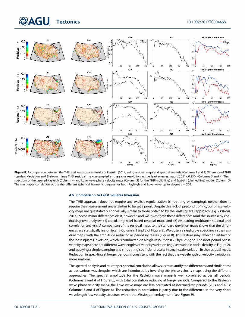
The THBI approach does not require any explicit regularization (smoothing or damping); neither does itrequire the measurement uncertainties to be set a priori. Despite this lack of preconditioning, our phase velo-city maps are qualitatively and visually similar to those obtained by the least squares approach [e.g., Ekström,2014]. Someminor differences exist, however, and we investigate these differences (and the sources) by con-ducting two analyses: (1) calculating pixel-based residual maps and (2) evaluating multitaper spectral andcorrelation analysis. A comparison of the residual maps to the standard deviation maps shows that the differ-ences are statistically insignificant (Columns 1 and 2 of Figure 8). We observe negligible speckling in the resi-dual maps, with the amplitude reducing as period increases (Figure 8). This feature may reflect an artifact ofthe least squares inversion, which is conducted on a high-resolution 0.25 by 0.25° grid. For short-period phasevelocity maps there are different wavelengths of velocity variation (e.g., see variable nodal density in Figure 2),and applying a single damping and smoothing coefficient results in small-scale variation in the residual maps.Reduction in speckling at longer periods is consistent with the fact that the wavelength of velocity variation ismore uniform.

The spectral analysis andmultitaper spectral correlation allows us to quantify the differences (and similarities)across various wavelengths, which are introduced by inverting the phase velocity maps using the differentapproaches. The spectral amplitude for the Rayleigh wave maps is well correlated across all periods(Columns 3 and 4 of Figure 8), with total correlation reducing at longer periods. Compared to the Rayleighwave phase velocity maps, the Love wave maps are less correlated at intermediate periods (20 s and 40 s;Columns 3 and 4 of Figure 8). The reduction in correlation is partly due to the difference in the very shortwavelength low velocity structure within the Mississippi embayment (see Figure 9).

Figure 8. A comparison between the THBI and least squares results of Ekström [2014] using residual maps and spectral analysis. (Columns 1 and 2) Difference of THBIstandard deviation and Ekstrom minus THBI residual maps resampled at the same resolution as the least squares maps (0.25° × 0.25°). (Columns 3 and 4) Thespectrum of the tapered Rayleigh (Column 4) and Love wave phase velocity maps (Column 3) for the THBI (solid line) and Ekström (dashed line) model. (Column 5)The multitaper correlation across the different spherical harmonic degrees for both Rayleigh and Love wave up to degree l = 200.

Tectonics 10.1002/2017TC004468

OLUGBOJI ET AL. BAYESIAN EVALUATION OF U.S. CRUSTAL MODELS 14

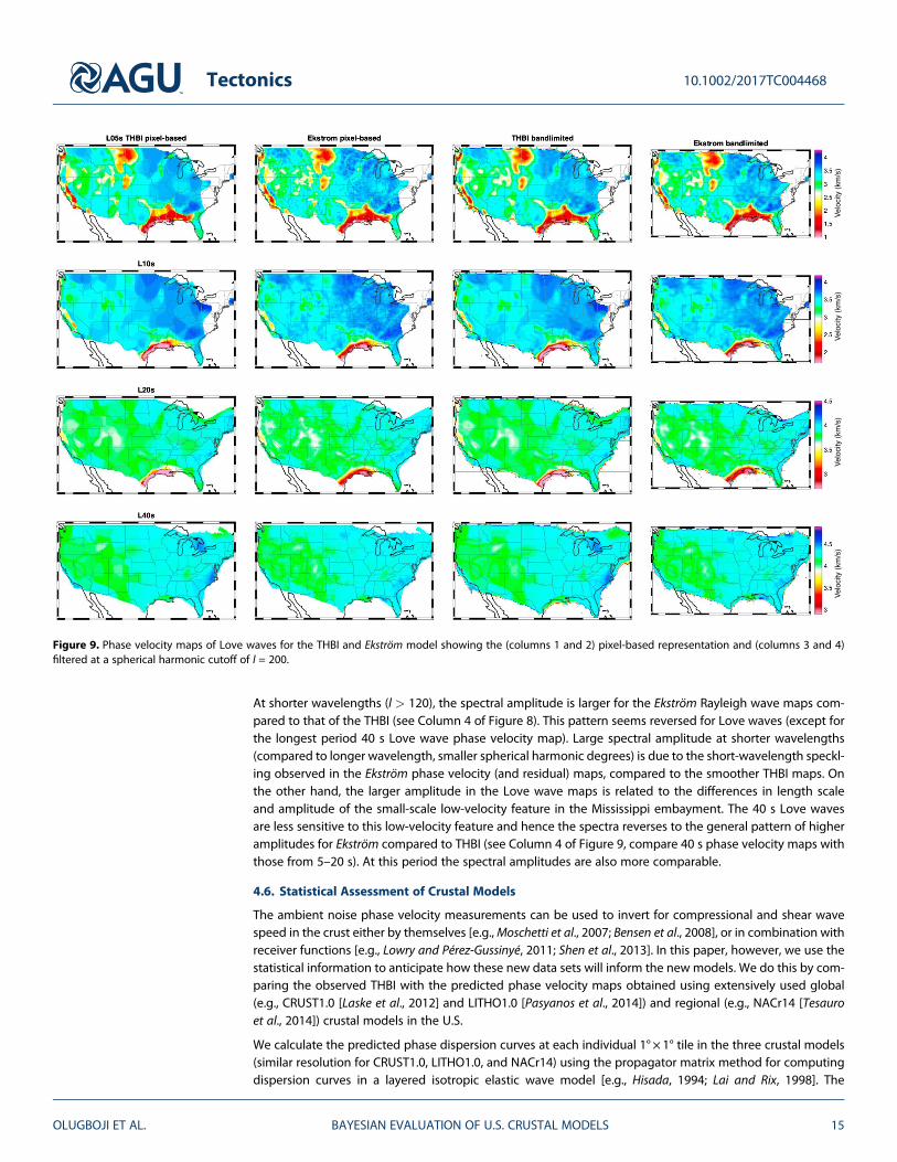
At shorter wavelengths (l > 120), the spectral amplitude is larger for the Ekström Rayleigh wave maps com-pared to that of the THBI (see Column 4 of Figure 8). This pattern seems reversed for Love waves (except forthe longest period 40 s Love wave phase velocity map). Large spectral amplitude at shorter wavelengths(compared to longer wavelength, smaller spherical harmonic degrees) is due to the short-wavelength speckl-ing observed in the Ekström phase velocity (and residual) maps, compared to the smoother THBI maps. Onthe other hand, the larger amplitude in the Love wave maps is related to the differences in length scaleand amplitude of the small-scale low-velocity feature in the Mississippi embayment. The 40 s Love wavesare less sensitive to this low-velocity feature and hence the spectra reverses to the general pattern of higheramplitudes for Ekström compared to THBI (see Column 4 of Figure 9, compare 40 s phase velocity maps withthose from 5–20 s). At this period the spectral amplitudes are also more comparable.

4.6. Statistical Assessment of Crustal Models

The ambient noise phase velocity measurements can be used to invert for compressional and shear wavespeed in the crust either by themselves [e.g.,Moschetti et al., 2007; Bensen et al., 2008], or in combination withreceiver functions [e.g., Lowry and Pérez-Gussinyé, 2011; Shen et al., 2013]. In this paper, however, we use thestatistical information to anticipate how these new data sets will inform the new models. We do this by com-paring the observed THBI with the predicted phase velocity maps obtained using extensively used global(e.g., CRUST1.0 [Laske et al., 2012] and LITHO1.0 [Pasyanos et al., 2014]) and regional (e.g., NACr14 [Tesauroet al., 2014]) crustal models in the U.S.

We calculate the predicted phase dispersion curves at each individual 1° × 1° tile in the three crustal models(similar resolution for CRUST1.0, LITHO1.0, and NACr14) using the propagator matrix method for computingdispersion curves in a layered isotropic elastic wave model [e.g., Hisada, 1994; Lai and Rix, 1998]. The

Figure 9. Phase velocity maps of Love waves for the THBI and Ekström model showing the (columns 1 and 2) pixel-based representation and (columns 3 and 4)filtered at a spherical harmonic cutoff of l = 200.

Tectonics 10.1002/2017TC004468

OLUGBOJI ET AL. BAYESIAN EVALUATION OF U.S. CRUSTAL MODELS 15

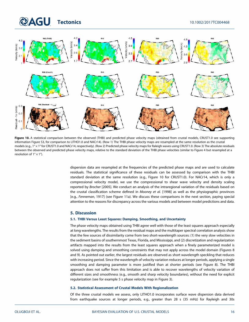
dispersion data are resampled at the frequencies of the predicted phase maps and are used to calculateresiduals. The statistical significance of these residuals can be assessed by comparison with the THBIstandard deviation at the same resolution (e.g., Figure 10 for CRUST1.0). For NACr14, which is only acompressional velocity model, we use the compressional to shear wave velocity and density scalingreported by Brocher [2005]. We conduct an analysis of the intraregional variation of the residuals based onthe crustal classification scheme defined in Mooney et al. [1998] as well as the physiographic provinces[e.g., Fenneman, 1917] (see Figure 11a). We discuss these comparisons in the next section, paying specialattention to the reasons for discrepancy across the various models and between model predictions and data.

5. Discussion5.1. THBI Versus Least Squares: Damping, Smoothing, and Uncertainty

The phase velocity maps obtained using THBI agree well with those of the least squares approach especiallyat long wavelengths. The results from the residual maps and the multitaper spectral correlation analysis showthat the few sources of dissimilarity come from two short-wavelength sources: (1) the very slow velocities inthe sediment basins of southernmost Texas, Florida, and Mississippi, and (2) discretization and regularizationartifacts mapped into the results from the least squares approach when a finely parameterized model issolved using damping and smoothing constraints that may not apply across the model domain (Figures 8and 9). As pointed out earlier, the largest residuals are observed as short wavelength speckling that reduceswith increasing period. Since the wavelength of velocity variation reduces at longer periods, applying a singlesmoothing and damping parameter is more justified than at shorter periods (see Figure 8). The THBIapproach does not suffer from this limitation and is able to recover wavelengths of velocity variation ofdifferent sizes and smoothness (e.g., smooth and sharp velocity boundaries), without the need for explicitregularization (see for example 5 s phase velocity map in Figure 3).

5.2. Statistical Assessment of Crustal Models With Regionalization

Of the three crustal models we assess, only LITHO1.0 incorporates surface wave dispersion data derivedfrom earthquake sources at longer periods, e.g., greater than 28 s (35 mHz) for Rayleigh and 30s

Figure 10. A statistical comparison between the observed (THBI) and predicted phase velocity maps (obtained from crustal models, CRUST1.0 see supportinginformation Figure S3, for comparison to LITHO1.0 and NACr14). (Row 1) The THBI phase velocity maps are resampled at the same resolution as the crustalmodels (e.g., 1° × 1° for CRUST1.0 and NACr14, respectively). (Row 2) Predicted phase velocity maps for Raleigh waves using CRUST1.0. (Row 3) The absolute residualsbetween the observed and predicted phase velocity maps, relative to the standard deviation of the THBI phase velocities (similar to Figure 4 but resampled at aresolution of 1° × 1°).

Tectonics 10.1002/2017TC004468

OLUGBOJI ET AL. BAYESIAN EVALUATION OF U.S. CRUSTAL MODELS 16

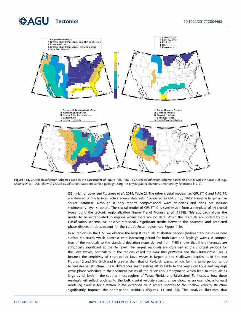
(33 mHz) for Love [see Pasyanos et al., 2014, Table 2]. The other crustal models, i.e., CRUST1.0 and NACr14,are derived primarily from active source data sets. Compared to CRUST1.0, NACr14 uses a larger activesource database, although it only reports compressional wave velocities and does not includesedimentary layer structure. The crustal model of CRUST1.0 is synthesized from a template of 14 crustaltypes (using the tectonic regionalization Figure 11a of Mooney et al. [1998]). This approach allows themodel to be extrapolated to regions where there are no data. When the residuals are sorted by thisclassification scheme, we observe statistically significant misfits between the observed and predictedphase dispersion data, except for the Late Archean region (see Figure 11b).

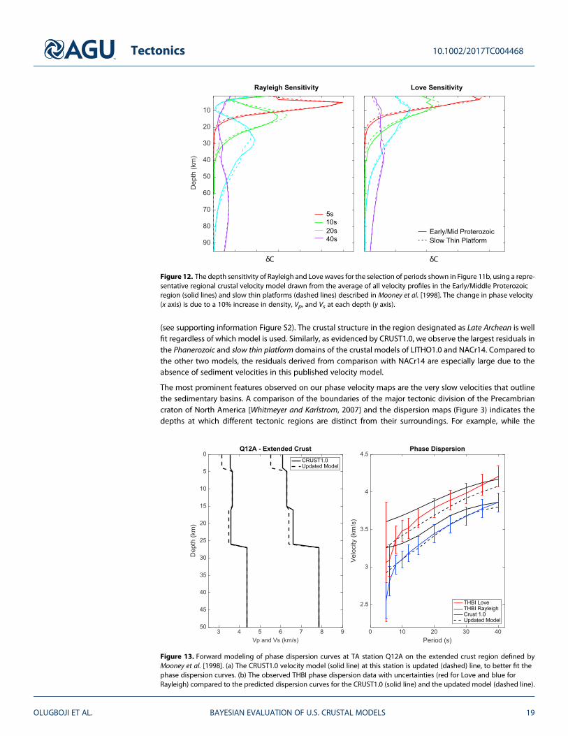
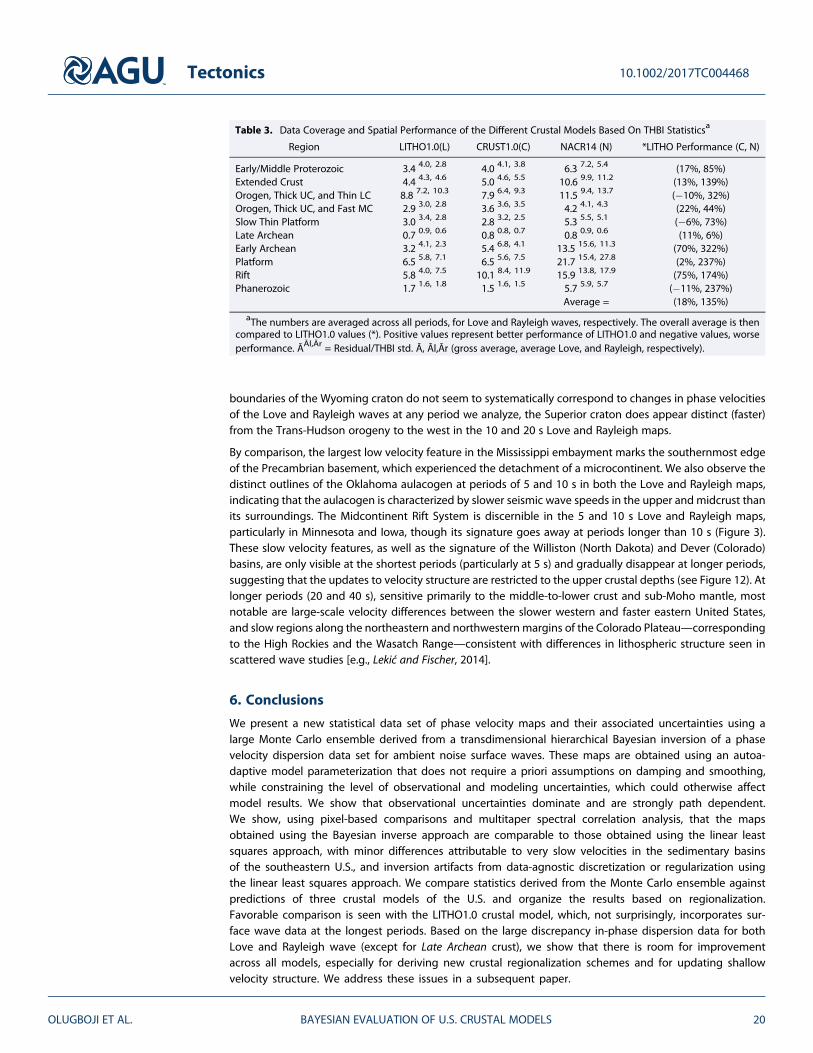
In all regions in the U.S., we observe the largest residuals at shorter periods (sedimentary basins or nearsurface structure), which decrease with increasing period for both Love and Rayleigh waves. A compar-ison of the residuals to the standard deviation maps derived from THBI shows that the differences arestatistically significant at the 3σ level. The largest residuals are observed at the shortest periods forthe Love waves, particularly in the regions called the slow thin platforms and the Phanerozoic. This isbecause the sensitivity of short-period Love waves is larger at the shallowest depths (<10 km, seeFigures 12 and S4a–S4d) and is greater than that of Rayleigh waves, which, for the same period, tendsto feel deeper structure. These differences are therefore attributable to the very slow Love and Rayleighwave phase velocities in the sediment basins of the Mississippi embayment, which lead to residuals aslarge as 1.1 km/s in the southernmost regions of Texas, Florida and Mississippi. To illustrate how theseresiduals will reflect updates to the bulk crustal velocity structure, we show, as an example, a forwardmodeling exercise for a station in the extended crust, where updates to the shallow velocity structuresignificantly improve the short-period residuals (Figures 13 and S5). This analysis illustrates that

Figure 11a. Crustal classification schemes used in the assessment of Figure 11b. (Row 1) Crustal classification scheme based on crustal types in CRUST1.0 [e.g.,Mooney et al., 1998]. (Row 2) Crustal classification based on surface geology using the physiographic divisions described by Fenneman [1917].

Tectonics 10.1002/2017TC004468

OLUGBOJI ET AL. BAYESIAN EVALUATION OF U.S. CRUSTAL MODELS 17

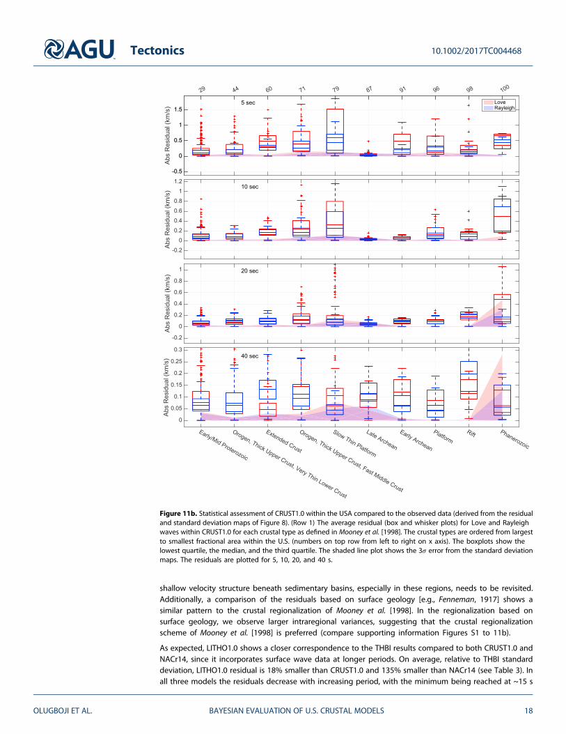
shallow velocity structure beneath sedimentary basins, especially in these regions, needs to be revisited.Additionally, a comparison of the residuals based on surface geology [e.g., Fenneman, 1917] shows asimilar pattern to the crustal regionalization of Mooney et al. [1998]. In the regionalization based onsurface geology, we observe larger intraregional variances, suggesting that the crustal regionalizationscheme of Mooney et al. [1998] is preferred (compare supporting information Figures S1 to 11b).

As expected, LITHO1.0 shows a closer correspondence to the THBI results compared to both CRUST1.0 andNACr14, since it incorporates surface wave data at longer periods. On average, relative to THBI standarddeviation, LITHO1.0 residual is 18% smaller than CRUST1.0 and 135% smaller than NACr14 (see Table 3). Inall three models the residuals decrease with increasing period, with the minimum being reached at ~15 s

Figure 11b. Statistical assessment of CRUST1.0 within the USA compared to the observed data (derived from the residualand standard deviation maps of Figure 8). (Row 1) The average residual (box and whisker plots) for Love and Rayleighwaves within CRUST1.0 for each crustal type as defined in Mooney et al. [1998]. The crustal types are ordered from largestto smallest fractional area within the U.S. (numbers on top row from left to right on x axis). The boxplots show thelowest quartile, the median, and the third quartile. The shaded line plot shows the 3σ error from the standard deviationmaps. The residuals are plotted for 5, 10, 20, and 40 s.

Tectonics 10.1002/2017TC004468

OLUGBOJI ET AL. BAYESIAN EVALUATION OF U.S. CRUSTAL MODELS 18

(see supporting information Figure S2). The crustal structure in the region designated as Late Archean is wellfit regardless of which model is used. Similarly, as evidenced by CRUST1.0, we observe the largest residuals inthe Phanerozoic and slow thin platform domains of the crustal models of LITHO1.0 and NACr14. Compared tothe other two models, the residuals derived from comparison with NACr14 are especially large due to theabsence of sediment velocities in this published velocity model.

The most prominent features observed on our phase velocity maps are the very slow velocities that outlinethe sedimentary basins. A comparison of the boundaries of the major tectonic division of the Precambriancraton of North America [Whitmeyer and Karlstrom, 2007] and the dispersion maps (Figure 3) indicates thedepths at which different tectonic regions are distinct from their surroundings. For example, while the

Figure 12. The depth sensitivity of Rayleigh and Love waves for the selection of periods shown in Figure 11b, using a repre-sentative regional crustal velocity model drawn from the average of all velocity profiles in the Early/Middle Proterozoicregion (solid lines) and slow thin platforms (dashed lines) described in Mooney et al. [1998]. The change in phase velocity(x axis) is due to a 10% increase in density, Vp, and Vs at each depth (y axis).

Figure 13. Forward modeling of phase dispersion curves at TA station Q12A on the extended crust region defined byMooney et al. [1998]. (a) The CRUST1.0 velocity model (solid line) at this station is updated (dashed) line, to better fit thephase dispersion curves. (b) The observed THBI phase dispersion data with uncertainties (red for Love and blue forRayleigh) compared to the predicted dispersion curves for the CRUST1.0 (solid line) and the updated model (dashed line).

Tectonics 10.1002/2017TC004468

OLUGBOJI ET AL. BAYESIAN EVALUATION OF U.S. CRUSTAL MODELS 19

boundaries of the Wyoming craton do not seem to systematically correspond to changes in phase velocitiesof the Love and Rayleigh waves at any period we analyze, the Superior craton does appear distinct (faster)from the Trans-Hudson orogeny to the west in the 10 and 20 s Love and Rayleigh maps.

By comparison, the largest low velocity feature in the Mississippi embayment marks the southernmost edgeof the Precambrian basement, which experienced the detachment of a microcontinent. We also observe thedistinct outlines of the Oklahoma aulacogen at periods of 5 and 10 s in both the Love and Rayleigh maps,indicating that the aulacogen is characterized by slower seismic wave speeds in the upper and midcrust thanits surroundings. The Midcontinent Rift System is discernible in the 5 and 10 s Love and Rayleigh maps,particularly in Minnesota and Iowa, though its signature goes away at periods longer than 10 s (Figure 3).These slow velocity features, as well as the signature of the Williston (North Dakota) and Dever (Colorado)basins, are only visible at the shortest periods (particularly at 5 s) and gradually disappear at longer periods,suggesting that the updates to velocity structure are restricted to the upper crustal depths (see Figure 12). Atlonger periods (20 and 40 s), sensitive primarily to the middle-to-lower crust and sub-Moho mantle, mostnotable are large-scale velocity differences between the slower western and faster eastern United States,and slow regions along the northeastern and northwestern margins of the Colorado Plateau—correspondingto the High Rockies and the Wasatch Range—consistent with differences in lithospheric structure seen inscattered wave studies [e.g., Lekić and Fischer, 2014].

6. Conclusions

We present a new statistical data set of phase velocity maps and their associated uncertainties using alarge Monte Carlo ensemble derived from a transdimensional hierarchical Bayesian inversion of a phasevelocity dispersion data set for ambient noise surface waves. These maps are obtained using an autoa-daptive model parameterization that does not require a priori assumptions on damping and smoothing,while constraining the level of observational and modeling uncertainties, which could otherwise affectmodel results. We show that observational uncertainties dominate and are strongly path dependent.We show, using pixel-based comparisons and multitaper spectral correlation analysis, that the mapsobtained using the Bayesian inverse approach are comparable to those obtained using the linear leastsquares approach, with minor differences attributable to very slow velocities in the sedimentary basinsof the southeastern U.S., and inversion artifacts from data-agnostic discretization or regularization usingthe linear least squares approach. We compare statistics derived from the Monte Carlo ensemble againstpredictions of three crustal models of the U.S. and organize the results based on regionalization.Favorable comparison is seen with the LITHO1.0 crustal model, which, not surprisingly, incorporates sur-face wave data at the longest periods. Based on the large discrepancy in-phase dispersion data for bothLove and Rayleigh wave (except for Late Archean crust), we show that there is room for improvementacross all models, especially for deriving new crustal regionalization schemes and for updating shallowvelocity structure. We address these issues in a subsequent paper.

Table 3. Data Coverage and Spatial Performance of the Different Crustal Models Based On THBI Statisticsa

Region LITHO1.0(L) CRUST1.0(C) NACR14 (N) *LITHO Performance (C, N)

Early/Middle Proterozoic 3.4 4.0, 2.8 4.0 4.1, 3.8 6.3 7.2, 5.4 (17%, 85%)Extended Crust 4.4 4.3, 4.6 5.0 4.6, 5.5 10.6 9.9, 11.2 (13%, 139%)Orogen, Thick UC, and Thin LC 8.8 7.2, 10.3 7.9 6.4, 9.3 11.5 9.4, 13.7 (�10%, 32%)Orogen, Thick UC, and Fast MC 2.9 3.0, 2.8 3.6 3.6, 3.5 4.2 4.1, 4.3 (22%, 44%)Slow Thin Platform 3.0 3.4, 2.8 2.8 3.2, 2.5 5.3 5.5, 5.1 (�6%, 73%)Late Archean 0.7 0.9, 0.6 0.8 0.8, 0.7 0.8 0.9, 0.6 (11%, 6%)Early Archean 3.2 4.1, 2.3 5.4 6.8, 4.1 13.5 15.6, 11.3 (70%, 322%)Platform 6.5 5.8, 7.1 6.5 5.6, 7.5 21.7 15.4, 27.8 (2%, 237%)Rift 5.8 4.0, 7.5 10.1 8.4, 11.9 15.9 13.8, 17.9 (75%, 174%)Phanerozoic 1.7 1.6, 1.8 1.5 1.6, 1.5 5.7 5.9, 5.7 (�11%, 237%)

Average = (18%, 135%)

aThe numbers are averaged across all periods, for Love and Rayleigh waves, respectively. The overall average is thencompared to LITHO1.0 values (*). Positive values represent better performance of LITHO1.0 and negative values, worseperformance. ĀĀl,Ār = Residual/THBI std. Ā, Āl,Ār (gross average, average Love, and Rayleigh, respectively).

Tectonics 10.1002/2017TC004468

OLUGBOJI ET AL. BAYESIAN EVALUATION OF U.S. CRUSTAL MODELS 20

ReferencesAki, K. (1957), Space and time spectra of stationary stochastic waves, with special reference to microtremors, Bull. Earthquake Res. Inst., 35,

415–457, doi:http://hdl.handle.net/2261/11892.Bassin, C., G. Laske, and G. Masters (2000), The current limits of resolution for surface wave tomography in North America, Eos. Trans. AGU, 81

F897.Becker, T. W., and L. Boschi (2002), A comparison of tomographic and geodynamic mantle models, Geochem., Geophys., Geosyst., 3(1), 1003,

doi:10.1029/2001GC000168.Benoit, M. H., C. Ebinger, and M. Crampton (2014), Orogenic bending around a rigid Proterozoic magmatic rift beneath the Central

Appalachian Mountains, Earth Planet. Sci. Lett., 402, 197–208, doi:10.1016/j.epsl.2014.03.064.Bensen, G. D., M. H. Ritzwoller, M. P. Barmin, A. L. Levshin, F. Lin, M. P. Moschetti, N. M. Shapiro, and Y. Yang (2007), Processing seismic

ambient noise data to obtain reliable broad-band surface wave dispersionmeasurements, Geophys. J. Int., 169(3), 1239–1260, doi:10.1111/j.1365-246X.2007.03374.x.

Bensen, G. D., M. H. Ritzwoller, and N. M. Shapiro (2008), Broadband ambient noise surface wave tomography across the United States,J. Geophys. Res., 113, B05306, doi:10.1029/2007JB005248.

Bensen, G. D., M. H. Ritzwoller, and Y. Yang (2009), A 3-D shear velocity model of the crust and uppermost mantle beneath the United Statesfrom ambient seismic noise, Geophys. J. Int., 177, 1177–1196, doi:10.1111/j.1365-246X.2009.04125.x.

Bodin, T., and M. Sambridge (2009), Seismic tomography with the reversible jump algorithm, Geophys. J. Int., 178(3), 1411–1436, doi:10.1111/j.1365-246X.2009.04226.x.

Bodin, T., M. Sambridge, H. Tkalčić, P. Arroucau, K. Gallagher, and N. Rawlinson (2012a), Transdimensional inversion of receiver functions andsurface wave dispersion, J. Geophys. Res., 117, B02301, doi:10.1029/2011JB008560.

Bodin, T., M. Sambridge, N. Rawlinson, and P. Arroucau (2012b), Transdimensional tomography with unknown data noise, Geophys. J. Int.,189(3), 1536–1556, doi:10.1111/j.1365-246X.2012.05414.x.

Brocher, T. M. (2005), Empirical relations between elastic wavespeeds and density in the Earth’s crust, Bull. Seismol. Soc. Am., 95(6), 2081–2092,doi:10.1785/0120050077.

Christensen, N. I., and W. D. Mooney (1995), Seismic velocity structure and composition of the continental crust: A global view, J. Geophys.Res., 100, 9761–9788, doi:10.1029/95JB00259.

Dahlen, F. A., and F. J. Simons (2007), Spectral estimation on a sphere in geophysics and cosmology, Geophys. J. Int., 174(3), 774–807,doi:10.1111/j.1365-246X.2008.03854.x.

Dalton, C. A., and J. B. Gaherty (2013), Seismic anisotropy in the continental crust of northwestern Canada, Geophys. J. Int., 193(1), 338–348,doi:10.1093/gji/ggs108.

Ekström, G. (2014), Love and Rayleigh phase-velocity maps, 5–40 s, of the western and central USA from USArray data, Earth Planet. Sci. Lett.,402, 42–49, doi:10.1016/j.epsl.2013.11.022.

Ekström, G., G. A. Abers, and S. C. Webb (2009), Determination of surface-wave phase velocities across USArray from noise and Aki’s spectralformulation, Geophys. Res. Lett., 36, L18301, doi:10.1029/2009GL039131.

Fenneman, N. M. (1917), Physiographic subdivision of the United States, Proc. Natl. Acad. Sci. U.S.A., 3(1), 17, doi:10.1073/pnas.1207851.Foster, A., M. Nettles, and G. Ekstrom (2014), Overtone interference in Array-based Love-wave phase measurements, Bull. Seismol. Soc. Am.,

104(5), 2266–2277, doi:10.1785/0120140100.Galetti, E., A. Curtis, G. A. Meles, and B. Baptie (2015), Uncertainty loops in travel-time tomography from nonlinear wave physics, Phys. Rev.

Lett., 114(14), 148501, doi:10.1103/PhysRevLett.114.148501.Green, P. (1995), Reversible jump Markov chain Monte Carlo computation and Bayesian model determination, Biometrika, 82(4), 711–732,

doi:10.1093/biomet/82.4.711.Green, P. J. (2003), Trans-dimensional Markov chain Monte Carlo, in Highly Structured Stochastic Systems, vol. 27, edited by P. J. Green,

N. L. Hjort, and S. Richardson, pp. 179–198, Oxford Univ. Press, New York.Hans Wedepohl, K. (1995), The composition of the continental crust, Geochim. Cosmochim. Acta, 59(7), 1217–1232, doi:10.1016/0016-7037

(95)00038-2.Harig, C., K. W. Lewis, A. Plattner, and F. J. Simons (2015), A suite of software analyzes data on the sphere, Eos (Washington. DC), 96, 1–10,

doi:10.1029/2015EO025851.Hisada, Y. (1994), An efficient numerical method for computing synthetic seismograms for a layered half-space with sources and receivers at

close or same depths, Bull. Seismol. Soc. Am., 84(5), 1456–1472, doi:10.1007/PL00012546.Hopper, E., K. M. Fischer, L. S. Wagner, and R. B. Hawman (2017), Reconstructing the end of the Appalachian orogeny, Geology, 45(1), 15–18,

doi:10.1130/G38453.1.Huang, Y., V. Chubakov, F. Mantovani, R. L. Rudnick, and W. F. McDonough (2013), A reference Earth model for the heat-producing elements

and associated geoneutrino flux, Geochem., Geophys., Geosyst., 14, 2003–2029, doi:10.1002/ggge.20129.Lai, C. G., and G. J. Rix (1998), Simultaneous inversion of Rayleigh phase velocity and attenuation for near-surface site characterization, School

of Civ. and Environ. Eng., Ga. Inst. of Technol.Laske, G., G. Masters, Z. Ma, and M. E. Pasyanos (2012), CRUST 1.0: An updated global model of the Earth’s Crust, EGU Meet. Abstr., (EGU2012-

3743).Lekić, V., and K. M. Fischer (2014), Contrasting lithospheric signatures across the western United States revealed by Sp receiver functions,

Earth Planet. Sci. Lett., 402, 90–98, doi:10.1016/j.epsl.2013.11.026.Liang, C., and C. A. Langston (2008), Ambient seismic noise tomography and structure of eastern North America, J. Geophys. Res., 113, B03309,

doi:10.1029/2007JB005350.Lin, F., and B. Schmandt (2014), Upper crustal azimuthal anisotropy across the contiguous US determined by Rayleigh wave ellipticity,

Geophys. Res. Lett., 41, 8301–8307, doi:10.1002/2014GL062362.Long, M. D., A. Levander, and P. M. Shearer (2014), An introduction to the special issue of Earth and Planetary Science Letters on USArray

science, Earth Planet. Sci. Lett., 402, 1–5, doi:10.1016/j.epsl.2014.06.016.Lowry, A. R., and M. Pérez-Gussinyé (2011), The role of crustal quartz in controlling Cordilleran deformation, Nature, 471(7338), 353–357,

doi:10.1038/nature09912.Malinverno, A., and V. A. Briggs (2004), Expanded uncertainty quantification in inverse problems: Hierarchical Bayes and empirical Bayes,

Geophysics, 69(4), 1005–1016, doi:10.1190/1.1778243.Malinverno, A., and R. L. Parker (2006), Two ways to quantify uncertainty in geophysical inverse problems, Geophysics, 71(3), W15–W27,

doi:10.1190/1.2194516.

Tectonics 10.1002/2017TC004468

OLUGBOJI ET AL. BAYESIAN EVALUATION OF U.S. CRUSTAL MODELS 21

AcknowledgmentsThis work was made possible by grantsand support from the PackardFoundation and the National ScienceFoundation. The authors acknowledgethe University of Maryland supercom-puting resources (http://www.it.umd.edu/hpcc) made available for conduct-ing the research reported in this paper.We are grateful to Göran Ekström formaking the data set of ambient noisephase velocity measurements acrossthe EarthScope USArray freely availablefor download on his website: http://www.ldeo.columbia.edu/~ekstrom/. Weacknowledge the use of the followingsoftware: (1) transtomo, developed anddistributed by the Australian NationalUniversity at iearthsoftware.org. (2)mat_disperse, developed by Lai and Rix[1998], which was used to solve thesurface wave dispersion equation, and(3) Slepian_alpha, which was used toconduct spatiospectral analysis and isdeveloped and distributed by theSimons group at Princeton [e.g., Hariget al., 2015]. These software wereextended and modified for personal usein this study. In particular, the dispersionsoftware was extended to solve theLove dispersion problem. We alsoacknowledge many helpful discussionswith Roberta Rudnick, Alain Plattner,Scott Burdick, Raj Moulik, LaurenWaszek, Scott Wipperfurth, ErinCunningham, and Chao Gao. Tools forvisualization and resampling of theMonte Carlo ensemble can be obtainedfrom www.tolulopeolugboji.name/open-data.

Menke, W. (2012), Solution of the linear, Gaussian inverse problem, viewpoint 3, in Geophysical Data Analysis: Discrete Inverse Theory,pp. 89–114, Elsevier, doi:10.1016/B978-0-12-397160-9.00018-7.

Menke, W., and G. Jin (2015), Waveform fitting of cross spectra to determine phase velocity using Aki’s formula, Bull. Seismol. Soc. Am., 105(3),1–9, doi:10.1785/0120140245.

Meschede, M., and B. Romanowicz (2015), Lateral heterogeneity scales in regional and global upper mantle shear velocity models, Geophys.J. Int., 200, 1076–1093, doi:10.1093/gji/ggu424.

Mooney, W. D., G. Laske, and T. G. Masters (1998), CRUST 5.1: A global crustal model at 5° × 5°, J. Geophys. Res., 103(B1), 727–747, doi:10.1029/97JB02122.

Moschetti, M. P., M. H. Ritzwoller, and N. M. Shapiro (2007), Surface wave tomography of the western United States from ambient seismicnoise: Rayleigh wave group velocity maps, Geochem., Geophys., Geosyst., 8, Q08010, doi:10.1029/2007GC001655.

Moschetti, M. P., M. H. Ritzwoller, F.-C. Lin, and Y. Yang (2010a), Crustal shear wave velocity structure of the western United States inferredfrom ambient seismic noise and earthquake data, J. Geophys. Res., 115, B10306, doi:10.1029/2010JB007448.

Moschetti, M. P., M. H. Ritzwoller, F. Lin, and Y. Yang (2010b), Seismic evidence for widespread western-US deep-crustal deformation causedby extension, Nature, 464(7290), 885–889, doi:10.1038/nature08951.

Nataf, H.-C., and Y. Ricard (1996), 3SMAC: An a priori tomographic model of the upper mantle based on geophysical modeling, Phys. EarthPlanet. Inter., 95(1–2), 101–122, doi:10.1016/0031-9201(95)03105-7.

Pasyanos, M. E., T. G. Masters, G. Laske, and Z. Ma (2014), LITHO1.0: An updated crust and lithospheric model of the Earth, J. Geophys. Res. SolidEarth, 119, 2153–2173, doi:10.1002/2013JB010626.

Pollitz, F. F., and W. D. Mooney (2014), Seismic structure of the Central US crust and shallow upper mantle: Uniqueness of the Reelfoot Rift,Earth Planet. Sci. Lett., 402(C), 157–166, doi:10.1016/j.epsl.2013.05.042.

Prieto, G. A., J. F. Lawrence, and G. C. Beroza (2009), Anelastic Earth structure from the coherency of the ambient seismic field, J. Geophys. Res.,114, B07303, doi:10.1029/2008JB006067.

Ray, A., D. L. Alumbaugh, G. M. Hoversten, and K. Key (2013), Robust and accelerated Bayesian inversion of marine controlled-source elec-tromagnetic data using parallel tempering, Geophysics, 78(6), E271–E280, doi:10.1190/geo2013-0128.1.

Rudnick, R. L., and S. Gao (2014), Composition of the continental crust, in Treatise on Geochemistry, vol. 4, pp. 1–51, Elsevier, San Diego, Calif.Sambridge, M., J. Braun, and H. McQueen (1995), Geophysical parametrization and interpolation of irregular data using natural neighbours,

Geophys. J. Int., 122(3), 837–857, doi:10.1111/j.1365-246X.1995.tb06841.x.Sambridge, M., K. Gallagher, A. Jackson, and P. Rickwood (2006), Trans-dimensional inverse problems, model comparison and the evidence,

Geophys. J. Int., 167(2), 528–542, doi:10.1111/j.1365-246X.2006.03155.x.Sambridge, M., T. Bodin, K. Gallagher, and H. Tkalcic (2012), Transdimensional inference in the geosciences, Philos. Trans. R. Soc. A Math. Phys.

Eng. Sci., 371(1984), 201105474, doi:10.1098/rsta.2011.0547.Saygin, E., P. R. Cummins, A. Cipta, R. Hawkins, R. Pandhu, J. Murjaya, Masturyono, M. Irsyam, S. Widiyantoro, and B. L. N. Kennett (2016),

Imaging architecture of the Jakarta Basin, Indonesia with transdimensional inversion of seismic noise, Geophys. J. Int., 204(2), 918–931,doi:10.1093/gji/ggv466.

Schmandt, B., F. Lin, and K. E. Karlstrom (2015), Distinct crustal isostasy trends east and west of the Rocky Mountain front, Geophys. Res. Lett.,42, 10,290–10,298, doi:10.1002/2015GL066593.

Shapiro, N. M. (2005), High-resolution surface-wave tomography from ambient seismic noise, Science, 307(5715), 1615–1618, doi:10.1126/science.1108339.

Shen, W., and M. H. Ritzwoller (2016), Crustal and uppermost mantle structure beneath the United States, J. Geophys. Res. Solid Earth, 121,4306–4342, doi:10.1002/2016JB012887.

Shen, W., M. H. Ritzwoller, and V. Schulte-Pelkum (2013), A 3-Dmodel of the crust and uppermost mantle beneath the central and western USby joint inversion of receiver functions and surface wave dispersion, J. Geophys. Res. Solid Earth, 118, 262–276, doi:10.1029/2012JB009602.

Simons, F. J., F. A. Dahlen, and M. A. Wieczorek (2006), Spatiospectral concentration on a sphere, SIAM Rev., 48(3), 504–536, doi:10.1137/S0036144504445765.

Stachnik, J. C., K. Dueker, D. L. Schutt, and H. Yuan (2008), Imaging Yellowstone plume-lithosphere interactions from inversion of ballistic anddiffusive Rayleigh wave dispersion and crustal thickness data, Geochem., Geophys., Geosyst., 9, Q06004, doi:10.1029/2008GC001992.

Tesauro, M., M. K. Kaban, W. D. Mooney, and S. Cloetingh (2014), NACr14: A 3D model for the crustal structure of the North AmericanContinent, Tectonophysics, 631, 65–86, doi:10.1016/j.tecto.2014.04.016.

Tsai, V. C., and M. P. Moschetti (2010), An explicit relationship between time-domain noise correlation and spatial autocorrelation (SPAC)results, Geophys. J. Int., 182(1), 454–460, doi:10.1111/j.1365-246X.2010.04633.x.

Whitmeyer, S. J., and K. E. Karlstrom (2007), Tectonic model for the Proterozoic growth of North America, Geosphere, 3(4), 220–259,doi:10.1130/GES00055.1.

Yang, Y., M. H. Ritzwoller, F. C. Lin, M. P. Moschetti, and N. M. Shapiro (2008), Structure of the crust and uppermost mantle beneath thewestern United States revealed by ambient noise and earthquake tomography, J. Geophys. Res., 113, B12310, doi:10.1029/2008JB005833.

Yang, Y., M. H. Ritzwoller, and C. H. Jones (2011), Crustal structure determined from ambient noise tomography near the magmatic centers ofthe Coso region, southeastern California, Geochem., Geophys., Geosyst., 12, Q02009, doi:10.1029/2010GC003362.

Young, M., N. Rawlinson, and T. Bodin (2013), Transdimensional inversion of ambient seismic noise for 3D shear velocity structure of theTasmanian crust, Geophysics, 78(3), WB49–WB62, doi:10.1190/geo2012-0356.1.

Yuan, H. (2015), Secular change in Archaean crust formation recorded in Western Australia, Nat. Geosci., 8(10), 808–813, doi:10.1038/ngeo2521.

Zhang, H., et al. (2016), Distinct crustal structure of the North American midcontinent rift from Pwave receiver functions, J. Geophys. Res. SolidEarth, 121, 8136–8153, doi:10.1002/2016JB013244.

Tectonics 10.1002/2017TC004468

OLUGBOJI ET AL. BAYESIAN EVALUATION OF U.S. CRUSTAL MODELS 22