a spatial model to aggregate point-source and nonpoint-source water-quality data for large areas

Computers & Geosciences Vol. 18, No. 8, pp. 1055-1073, 1992 0098-3004/92 $5.00 + 0.00 Printed in Great Britain Pergamon Press Ltd

A SPATIAL MODEL TO AGGREGATE POINT-SOURCE A N D NONPOINT-SOURCE WATER-QUALITY DATA FOR

LARGE AREAS

DALE A. WHITE, 1 RICHARD A. SMITH, 2 CURTIS V. PRICE, 3 RICHARD B. ALEXANDER, 2 and KEITH W. ROBINSON 3

I School of Natural Resources, The Ohio State University, Columbus, OH 43210-1085, 2U.S. Geological Survey, Water Resources Division, Reston, VA 22092, and 3U.S. Geological Survey, Water Resources

Division, West Trenton, NJ 08628, U.S.A.

Abstract--More objective and consistent methods are needed to assess water quality for large areas. A spatial model, one that capitalizes on the topologic relationships among spatial entities, to aggregate pollution sources from upstream drainage areas is described that can be implemented on land surfaces having heterogeneous water-pollution effects. An infrastructure of stream networks and drainage basins, derived from 1:250,000-scale digital-elevation models, define the hydrologic system in this spatial model. The spatial relationships between point- and nonpoint pollution sources and measurement locations are referenced to the hydrologic infrastructure with the aid of a geographic information system. A maximum-branching algorithm has been developed to simulate the effects of distance from a pollutant source to an arbitrary downstream location, a function traditionally employed in deterministic water quality models.

Key Words: Maximum-branching algorithm, Drainage networks, Distance decay, Water quality, Geographic information systems.

INTRODUCTION

Because of the growing concern with large-scale environmental problems, such as nonpoint-source pollution of streams, acid rain, and climate change, the need for regional impact assessment is critical. In order to detect and ameliorate the effects of large- scale environmental problems, the development of new monitoring and assessment methods will be required (Science Advisory Board, 1988). Impacts which may be significant locally can accumulate across space to cause substantial environmental degradation (Johnston and others, 1988). Surface water quality is one such example. A major problem in assessing the effects of anthropogenic impacts on regional surface water quality has been the difficulty in obtaining reliable information on cause and effect relationships for a representative sample of stream segments in a region (Cohen, Alley, and Wilber, 1988; U.S. General Accounting Office, 1986).

Cokriging has been one method used to assess regional stream quality (Jager, Sale, and Schmoyer, 1990). However for kriging techniques to be appli- cable on a regional scale, measurement data should exhibit spatial autocorrelation in multiple dimensions and for distances that are as large as the smallest two or three lag intervals. Most anthropogenic influences on stream quality do not operate in the full two- dimensional landscape. If spatial autocorrelation exists mainly along preferred flow paths, then a regional model must account for the linkage of pollution sources and pollution sinks. Johnston and others

(1988) attempt to perform this linkage by relating wetland position in the drainage basin to water quality. However, they compare the stream order (hierarchical magnitude of stream topology) at the wetland mouth to order at the basin mouth as a method for weighing the positional impact of each wetland.

Past efforts to deterministically model water quality tended to focus on small drainage areas or on segments of rivers. Recently developed deterministic models are distributed spatially using grid cells to discretize the domain (e.g. AGNPS, Young and others, 1989; ANSWERS, Beasley, Huggins, and Monke, 1980) or can consider agricultural domains of spatial extents as large as 600-800 km 2 (e.g. SWRRB- WQ, Arnold and others, 1992). More effort is needed to characterize water-quality conditions for large regions that aggregate measurements from both point- and nonpoint-source impacts originating from both urbanized and agricultural land uses. Urbanized land uses were associated with maximum phosphorus concentrations in an agricultural drainage basin in eastern Illinois, U.S.A. (Osborne and Wiley, 1988). A water-quality modeling framework is proposed which: (1) encompasses large and diverse areas; (2) combines point and diffuse (nonpoint) sources of pollution; (3) links, explicitly, pollution impacts, and sinks via stream topology and geometry; and (4) employs existing inventories of water-quality data.

A spatial model exploits the topologic relationships among point, line, and polygon entities. The model was designed for large areas (e.g. the size of U.S.

1055

1056 D.A. Wnn'E and others

States, 104-106 km 2) but can be employed essentially on any size drainage basin. Its versatility is the result of the recognition of a topological and Iocational structure of pollution sources and sinks rather than the spatial resolution of land-surface characteristics, assuming these entities can be identified at a particular spatial scale. The spatial model employs analysis tools and data structures present in vector-based geographic information systems (GIS) and the extraction of drainage-basin morphometry from digital- elevation data. Compared to a grid cell approach for deterministically modeling water quality, the vector- based model structure offers a more precise representation of channel dimensions (e.g. length, slope, and topology) and a more accurate determination of the shortest path in a network, given constraints of direction and branching.

MODEL DEVELOPMENT

Dawdy (1967) states that for hydrologic models to be practical and efficient for prediction, they should balance simplicity with completeness. The development of a regional model of water quality must be detailed enough to account for a large diversity of pollution impacts arising from urbanized and rural land uses. Generally, the data requirements of deterministic models limit their use for large domains. For example, SWRRB-WQ (Arnold and others, 1992) requires specific channel characteristics for flood routing (e.g. top and bottom width, depth, and roughness). A spatial model is proposed that offers some degree of determinism by considering channel length (and slope) and provides a data and topological structure that potentially could be used for aiding the solution of routing and other process equations included in deterministic models.

Each of the four sections of this paper address several components in the overall model design (Fig. 1). The Overview describes in general terms how the domain is partitioned into elemental units and how water-quality attributes are assigned. A discussion of the deterministic components of the spatial model--pollutant decay and water-quality predictor formulation--completes the Overview. The second section considers the extraction of drainage networks and divides from digital elevation models and the inconsistencies of the extracted systems. A descrip- tion of an algorithm designed for upstream traversal of a drainage network, along with program requirements, comprises the third section of the paper. The paper concludes with a discussion of the versatility of this model for deterministic and statistical water- quality modeling. Other techniques which could be used in association also are briefly considered.

Overview

Partitioning of the domain into subbasin elements. Regional characterization of water quality encompasses spatial domains which consist of complex

mixtures of surface and subsurface attributes. These attributes consist of land cover, soil hydrologic parameters, terrain aspect and slope, and land use and their derivatives. Land use can be characterized further by human population density and the location of point-source discharges. By discretizing the spatial domain into smaller polygonal units, the complexity of land-surface characterization within any given unit is reduced. The scale of the discretization is appropriate when the critical components of the hydrologic flow regime are represented. Band (1989) advises that drainage basin response is captured when the proportion of topographic and surface cover variance that exists between units is maximized and the proportion that exists within units is minimized. Because patterns of land surface and subsurface homogeneity tend to follow drainage divides (Band, 1989), we apply the drainage subbasin as the primary unit of discretization.

Assignment of point-source and nonpoint-source attributes. If we consider the drainage basin as a method of discretization (a polygon), the land-surface attributes (associated with point, line, and polygon entities) contained within each subbasin can be identified by their cartographic intersection with the subbasin polygon. The type of cartographic intersection employed here considers the overlay of two sets of map features with the resultant map consisting of all features of the first map plus those features in the second map that lie within the domain of the first map.

Nonconservative transport of pollutants. The deliv- ery of pollutants to downstream locations occurs in two distinct phases: (1) land-to-stream, where overland and subsurface flow operate, and (2) in-channel, where a variety of liquid-phase and depositional processes operate. Fundamental differences exist in the chemical environment of these phases. In the surface phase, subaqueous conditions exist and there is temporal variability in available moisture. In the channel-flow phase, biogeochemical processes vary dramatically between terrestrial and aquatic environ- ments (Phillips, 1988). When pollutants wash from land to a drainage basin outlet, they are exposed to processes of decay. Pollutants can be added or sub- tracted by vegetation or other matter, become sorbed onto sediment, or be deposited and stored for variable lengths of time. These losses occur on the land surface, in soil, or in the water.

The spatial model developed here is based on an infrastructure of subbasins connected by stream reaches. A reach is defined as one segment of a drainage system generally extending from one stream junction to another. In this representation of pollution-flow processes, all upstream land-surface attributes are assigned to subbasin polygons (Figs. 1 and 2). However, the site-to-stream phase is ignored because material transport from upland areas to a subbasin outlet is not considered. We assume that all point and nonpoint sources of pollution occurring

Aggregating water-quality data for large areas 1057

I set area and confluence thresholds

sdiScretize study area into ub-basin polygons

] ~::::!convert to vector :II:I:.I::I:/?III:I:/IIIT:.III:I: I:.IIID

eliminate basins < min area

I~ one

I- eliminate basins w/o reaohes

I point-source (point-in-polygon) , / e.g., human population counts, ~ _ ~ build attribute table by inter- pipe discharge locations I Lsection with sub-isin polygons

nonpoint-source (polygon intersection) e.g., land use and land c o v e r

t digital elevation model (raster)

)

establish relation between network and sub-basins

1 establish initial nodes file

I I sot drainage density threshold

Gderive stream etwork )

I ::: .:.:.:.>..,...

1 refine network

C===n ) many ~ I

alculate weight proportion 1 or reaches which are part of ulti-reached sub-basins

(multiplication and summation) Figure 1. Conceptualization of spatial model for aggregating point- and nonpoint-source water-quality

data from upstream drainage areas.

within the subbasin make their impact at the subbasin outlet (Fig. 2). Because the size of the subbasin is depicted as the elemental unit, the error associated with the lack of site-to-stream representation is minimized. The model however, does account for downstream or channelized flow effects. Explicit representation of channel processes are made by calculation of the flow-path distance from an initial node (e.g. a water-quality monitoring station) to each upstream node colocated with a subbasin outlet.

Calculation of the flow-path distance is derived from a class of algorithms, termed tree-generating algorithms, that compute the traversal of a connected graph (Minieka, 1978). A graph is connected if there is a path between any two nodes of that graph (Fig. 3A). We examine a particular tree-generating algorithm, termed a maximum-branching algorithm (Edmonds, 1968), which considers the direction of each arc during traversal. The algorithm begins with a starting node and the graph is traversed from this node to all terminal nodes (Fig. 3B). The conditions for traversal are to determine the path with the

• bbasin outlet

• Point-source location ~ \ Initial

Nonpoint-source area

( ~ Locus of aggregation

Figure 2, Representation of pollution sources in drainage subbasin. Distance determination (d) is made from subbasin outlet to downstream node along flow path and then

adjusted to approximate center of subbasin.

1058 D.A. WHITE and others

l connected-graph G

O

O node or vertex

arc or edge

A

\ terminal nodes

[from-node to-node

arc direction and types I of reach-nodes

starting or initial node V~

connected-graph A

cycle in connected.graph C

C

starting or initi~

sub-graph A' of graph A D

Figure 3. Definition of graph terminology. A--Node and arcs of connected-graph G; B--node terminology of connected-graph A; C----existence of cycle in connected graph C; D---subgraph A' of graph

A. Cycle is path of length three or more arcs from node to itself.

minimum length and to move in one direction (upstream) only. Given the condition that a drainage network has no cycles (Fig. 3C), there exists one and only one unique path from a starting node to each node in the graph. This study describes a method for traversing a stream network from multiple starting

nodes with the possibility that some or all of the starting nodes exist in subgraphs of the complete drainage work (Fig. 3D).

Model formulation. Traversal of a stream network yields a cumulative-distance term which will be represented as a surrogate for the time it takes a


pollutant to decay from entry into the stream system to its point of measurement. Cumulative distance is the basis for calculating predictors of water quality. The point- and nonpoint-source pollution impacts situated upstream of an initial node comprise the initial loads of various pollutants. By combining distance effects and initial pollutant load, the formulation of a water-quality predictor variable for an individual pollutant, sj0 at location j0, takes the form:

s~ = a ~ l*Ei~j(L,y. W,~) (1)

where

i = index of pollutant source-type including individual point sources (e.g. sewage treatment plants) and nonpoint sources (e.g. agricultural and diffuse urban activity);

j = subbasin index; j = (1,2,3 . . . . n) of n subbasins which lie upstream of the initial node located at j0;

sj0 = pollutant load (MT- t ) at initial node located at j0;

Q~ = flow or discharge (L 3 T- ~ ) of stream segment at location j0;

L U = load of a pollutant (MT- 1 ) originating from source i in subbasin j ; and,

W,j = weighing factor representing the nonconservative transport of a pollutant.

The L 0 for point-source pollutants are assumed to be known. L U for nonpoint-sources are estimated as

Lij = Ao. Yi (2) where

A u = area (L 2) of nonpoint-source or diffuse activity (e.g. the area of an impervious parking lot); and

Y,=yield (ML-2T -~) of the nonpoint-source pollutant type i.

Assuming nonconservative downstream transport of the pollutant according to a first-order reaction (Thomann and Mueller, 1987), then

W,j = exp (-k~,dj) (3) where

kl = decay constant (L -~); and dy = flow path length (L) from thejth subbasin to

location of the initial node at j0.

Assuming stream velocity to be constant, a first-order reaction is one in which the rate of loss of the substance is proportional to its concentration at any distance (Fig. 4). Other decay models may be substi- tuted for Equation (3) depending on the type of water-quality prediction to be made.

tThe particular DEM used is DMA DTED-1 (U.S. Geo- logical Survey, 1983, p. 36-40) sampled at a frequency of 3 arc-sec. At 40°N lat, the sampling resolution is approximately 90 m (N-S) by 70m (E-W). Using a bilinear interpolation algorithm, the elevation data were resampled to a 90 m square-grid.

- - i So o " f

P

do Distance, d (L) Figure 4. Decay of nonconservative substances in streams. s o represents initial load of pollutant discharged into channel

at distance d 0.

From Equations (1)-(3) the important components of this spatial model are the distance factor, dj, measured from each subbasin to a downstream initial node along a flow path, and the ability to aggregate spatially distributed pollution inputs from j = 1,2,3 . . . . n subbasins. Estimates of Q, L (for point-source pollutants) or A and Y (for nonpoint- source pollutants), and k are necessary for solution of Equation (1).

The hydrologic flow path is represented geometrically as a series of chained coordinate pairs--known as directed chains or arcs--that are connected at points of intersection, termed nodes. A procedure has been developed to traverse a connected and directed network in the upstream direction to determine the hydrologic distance from each initial node to all upstream subbasins. The maximum-branching algorithm accounts for the nesting of drainage basin hier- archies such that some subbasins may influence the water quality at more than one initial node (Fig. 3D).

Deriving subbasin divides and stream networks from digital-elevation models

To generate a meaningful representation of the surface hydrologic system, the network must be correct topologically and morphometrically. Once this network is constructed, a variety of land-surface characteristics can be referenced to it. A flow system of sources and sinks of water quality thus is represented via a stream and drainage divide network. Pollution sources can be represented geometrically by either polygons or points (depending on their diffuse nature). Each entity can be tagged with one or more attributes. Pollution sinks are represented by arcs or flow paths separating pollution sources and by nodes which are the arbitrary downstream locations where water-quality predictions are made.

Anchoring geographic data onto a stream and drainage divide network. Jenson and Domingue (1988) have developed an automated procedure for extracting drainage divides and stream networks from a digital elevation model (DEM). A DEM consists of a regularly spaced two-dimensional array of surface topographic elevations. DEMs are available at several map scales and corresponding accuracy levels. DEMt at a scale of 1:250,000 and a sampling

1060 D.A. WmT~ and others

distance of 90 m is employed in this spatial model. Using the Jenson and Domingue (1988) procedure, and establishing specified upstream area (flow accumulation) andflow confuence thresholds, the study area is partitioned into drainage subbasins at a specific scale. A confluence value (calculated as a A) indicates the increase in flow accumulation as each grid cell in the DEM drains to its downstream neighbor (Jenson and Domingue, 1988, p. 1598). The advantage of using an automated basin- and network-extraction routine is that the subbasin units can be set at a scale appropriate to the application (Band, 1989). Subbasins are determined with the Jenson and Domingue (1988) procedure from DEM in raster tbrmat. In raster format, the subbasins consist of aggregates of grid cells having a common identifier (Fig. 5). The grid-based subbasins are converted to a vector representation using a raster-to-vector conversion algorithm for polygons. Compared to other procedures for extracting topographic structure from DEMs (e.g. Fairfield and Leymarie, 1991; Band, 1986; or O'Callaghan and Mark, 1984), the Jenson and Domingue (1988) procedure is one that is available readily for handling artificial depressions existing in the topographic surface.

Stream networks are derived in a manner similar to extracting the subbasin divides. The drainage density of the stream network is established in this spatial model by using a threshold of flow accumulation. All grid cells with flow-accumulation values that exceed the threshold are labeled a stream cell. The grid of stream cells are translated to vector format using a

conversion procedure developed by Greenlee (1987) Greenlee's algorithm converts raster linework by first filling (at points of low connectivity) and then thin- ning a chain of grid cells to a single-cell width. This single-cell width of grid cells eventually yields a chain of coordinates.

The model goal was to ensure that each subbasin contained at least one stream reach so that all upstream land-surface attributes would be accounted for in the aggregation process. Therefore, when applying the drainage-net extraction procedure, it was necessary to lower the threshold for drainage density (100 grid cells) below that of the area and confluence thresholds for depicting subbasins (250 grid cells). Consequently, most subbasins in the study area contain more than one stream reach. The maximum- branching algorithm is designed to traverse all reaches within a multireach subbasin. As one reach segment is traversed, the subbasin attributes are weighted by a factor proportional to the ratio of the length of the traversed reach to the total length of all reaches within the given subbasin.

Conditioning the stream network and drainage -basin divide for model building. Because of geometrical differences in raster and vector representation of objects, polygon remnants or artifacts may exist in the translation to vector format when only four- connectedness is allowed (eight-connectedness would reduce the likelihood of these artifacts; Fig. 6A). Subbasins with convex peninsulas would lose the peninsula after the vector conversion. Subbasins with areas smaller than the threshold also occurred in the

2 2 2

2 2 2

~.~ ~ ,.::~: 2 2 2

i '~: 1 2 2 2 i ~ . " ~':::.:: , ~ :

~ : . ~ iii~"+" .~i';.'~.~i

~ 1 2 i~"' ~ , ' " ~P

• ~1 "~.~ 2 2 ~..,~

P17

P25

I P18

P2

P1

P3

P16 1

P4

P13 P6

P9

PIO

P12

P24

P23

P22

2

P21 P5

P20

P7

I P8

P19

P11

A B Figure 5. Raster (A) and vector (B) representations of drainage subbasin polygons• Pn represents node

connecting two arcs in polygon•


t

I 1 1

• : : 1 : : : : ~:::::~: : | ,

I, I , : : : : : : : : : : : : : : : : : : : : : : : : : : : i

" , , i : : : : : i :: ):i : : i : i i i : : i : i : i i i "

::: ] ] c; ....... i

four-connectedn ,ss 1 1

' I

raster vector eight-connectedness A

~ F , ~ detached polygons

L

2

1

I \ remainder space

B Figure 6. Polygon artifacts resulting from conversion of subbasin polygons to vector format; artifacts

result from (A) four-connectedness and (B) remainder-space problems.

remainder space that existed between two larger subbasins (Fig. 6B). To remove these polygon artifacts and to establish a realistic physical representation for discretizing the study area, all subbasins less than 2.025 km 2 (250 grid cells at 90 m resolution) were dissolved (the area of a subbasin was absorbed into an adjacent subbasin; Table 1).

To associate a subbasin polygon with a stream reach, the subbasin coverage was combined with the stream-network coverage using a cartographic intersection (Fig. 1). A second polygon dissolve was performed in particular situations where the subbasin did not enclose at least one stream reach (e.g. subbasins that exist on the study area boundary). The


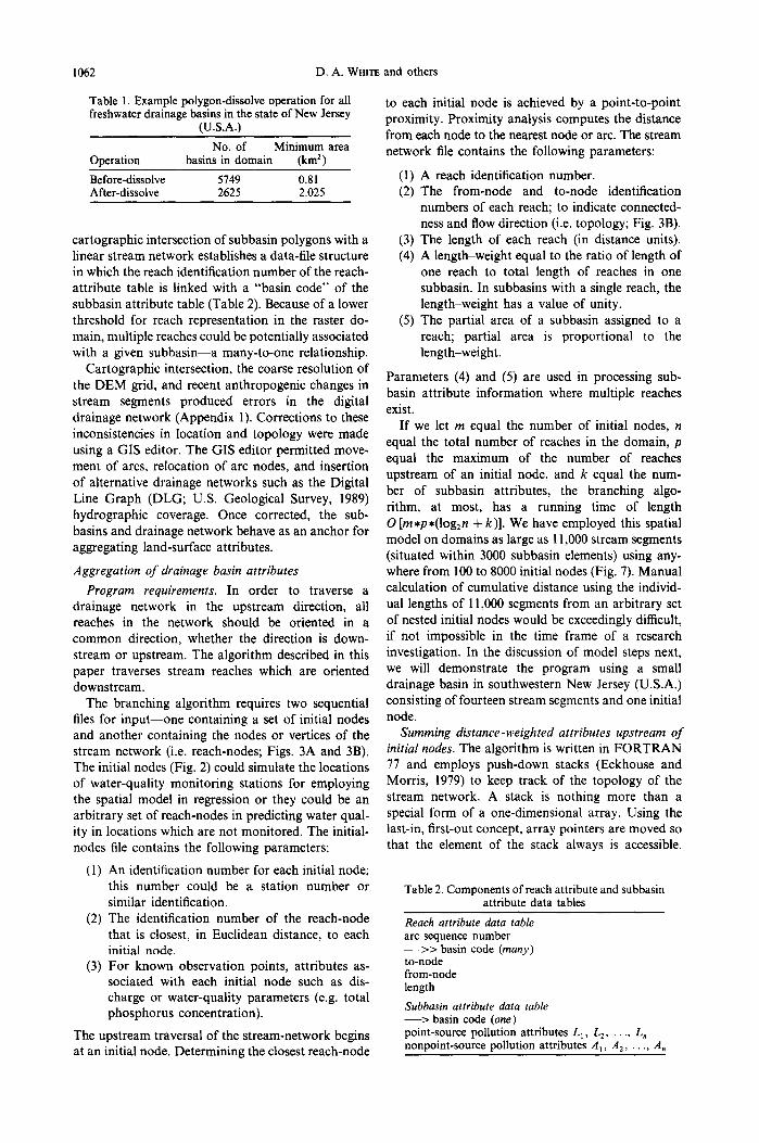
Table 1. Example polygon-dissolve operation for all freshwater drainage basins in the state of New Jersey

(U.S.A.)

No. of Minimum area Operation basins in domain (km 2)

Before-dissolve 5749 0.81 After-dissolve 2625 2.025

cartographic intersection of subbasin polygons with a linear stream network establishes a data-file structure in which the reach identification number of the reach- attribute table is linked with a "basin code" of the subbasin attribute table (Table 2). Because of a lower threshold for reach representation in the raster domain, multiple reaches could be potentially associated with a given subbasin--a many-to-one relationship.

Cartographic intersection, the coarse resolution of the DEM grid, and recent anthropogenic changes in stream segments produced errors in the digital drainage network (Appendix 1). Corrections to these inconsistencies in location and topology were made using a GIS editor. The GIS editor permitted move- ment of arcs, relocation of arc nodes, and insertion of alternative drainage networks such as the Digital Line Graph (DLG; U.S. Geological Survey, 1989) hydrographic coverage. Once corrected, the subbasins and drainage network behave as an anchor for aggregating land-surface attributes.

Aggregation of drainage basin attributes

Program requirements. In order to traverse a drainage network in the upstream direction, all reaches in the network should be oriented in a common direction, whether the direction is downstream or upstream. The algorithm described in this paper traverses stream reaches which are oriented downstream.

The branching algorithm requires two sequential files for input--one containing a set of initial nodes and another containing the nodes or vertices of the stream network (i.e. reach-nodes; Figs. 3A and 3B). The initial nodes (Fig. 2) could simulate the locations of water-quality monitoring stations for employing the spatial model in regression or they could be an arbitrary set of reach-nodes in predicting water quality in locations which are not monitored. The initial- nodes file contains the following parameters:

(1) An identification number for each initial node; this number could be a station number or similar identification.

(2) The identification number of the reach-node that is closest, in Euclidean distance, to each initial node.

(3) For known observation points, attributes associated with each initial node such as discharge or water-quality parameters (e.g. total phosphorus concentration).

The upstream traversal of the stream-network begins at an initial node. Determining the closest reach-node

to each initial node is achieved by a point-to-point proximity. Proximity analysis computes the distance from each node to the nearest node or arc. The stream network file contains the following parameters:

(1) A reach identification number. (2) The from-node and to-node identification

numbers of each reach; to indicate connectedness and flow direction (i.e. topology; Fig. 3B).

(3) The length of each reach (in distance units). (4) A length-weight equal to the ratio of length of

one reach to total length of reaches in one subbasin. In subbasins with a single reach, the length-weight has a value of unity.

(5) The partial area of a subbasin assigned to a reach; partial area is proportional to the length-weight.

Parameters (4) and (5) are used in processing subbasin attribute information where multiple reaches exist.

If we let m equal the number of initial nodes, n equal the total number of reaches in the domain, p equal the maximum of the number of reaches upstream of an initial node, and k equal the number of subbasin attributes, the branching algorithm, at most, has a running time of length 0 [m*p*(log2n + k)]. We have employed this spatial model on domains as large as 11,000 stream segments (situated within 3000 subbasin elements) using any- where from 100 to 8000 initial nodes (Fig. 7). Manual calculation of cumulative distance using the individual lengths of 11,000 segments from an arbitrary set of nested initial nodes would be exceedingly difficult, if not impossible in the time frame of a research investigation. In the discussion of model steps next, we will demonstrate the program using a small drainage basin in southwestern New Jersey (U.S.A.) consisting of fourteen stream segments and one initial node.

Summing distance-weighted attributes upstream of initial nodes. The algorithm is written in FORTRAN 77 and employs push-down stacks (Eckhouse and Morris, 1979) to keep track of the topology of the stream network. A stack is nothing more than a special form of a one-dimensional array. Using the last-in, first-out concept, array pointers are moved so that the element of the stack always is accessible.

Table 2. Components of reach attribute and subbasin attribute data tables

Reach attribute data table arc sequence number - - > > basin code (many) to-node from-node length

Subbasin attribute data table - - > basin code (one) point-source pollution attributes L m, L2, ..., L n nonpoint-source pollution attributes Am, A2, ..., A,


• . d l l . 5 " . ! =

,• "if

n • . , . : . . . , ; . . , . - •

• . " , • " " . " ~ , ' ' t , ~ • . , , - , r " . • . . 4 - - - /

.",r.~.: . ° • . , ; . . ' . ~ ~ - . • , . . , .. ~ . . . ~. o." . , . - ~ ~ . ~ . . ~ ~,- ,~ , , . . . . , .~ . . . , ... ~...: .. *-.,,4=_-~_ . , . . , ,,,- t..,.

I i : , , ¢ . . : . - - ' . : # . . - " ..,,~" ,~ / % .~ 1' .~'1 I } ' . ~ 1 I

0 5 10 miles . i I I I I

0 5 10 kilometers

D 75 74

I ~ I

4 1 - -

4 0 - -

3 9 - -

0 10 20 mi.ies 4 . ' . * . *

0 10 20 kilometers

I I Figure 7. Raritan River Basin, New Jersey, U,S.A., showing drainage network (A) and subbasin elements (B) derived from digital elevation data. Drainage network contains 1838 arc segments (mean length = 0.74 kin) and subbasin map consists of 663 unique polygons (mean area = 3.32 km2). C--Digital map of 1141 arc nodes used as initial locations for branching algorithm. Nodes represent downstream vertex for subset of 1838 arc segments in (A) which have cumulative drainage area > 2.0 km ~. D--Outline of study area (polygon inside coastline; New Jersey) for which spatial model has been applied (see text)

and showing relative position of Raritan Basin (shaded).

Source code for the complete traversal and aggregation program is contained in Appendix 2 (each step described here is identified in the main program).

Step 1. Network traversal and basin-attribute aggregation begins by searching the stream network file for all to-node numbers which match the reach-

node number associated with the first initial node (Fig. 8A).

Step 2. The identification numbers of the reach or reaches (in the situation of junctions) associated with the to-node matches are pushed onto a memory stack along with a corresponding cumulative distance term (Fig. 8B).

CAGEO 18/8---1

1064 D.A. WroTE et al.

For reaches which are attached to the initial node, the cumulative distance is equal to the length of that reach. As the network is traversed further, the cumulative distance associated with reaches situated at higher levels in the graph is equal to the flow-path length from the initial node to the to-node of any given reach.

Step 3. When a junction is encountered, all reaches which join at that junction are pushed onto the stack (Fig. 8A). Here search is breadth-first where one generation of child nodes in the subgraph is ex- hausted before moving down to the next generation (Fisher, 1990). Then the reach which was last placed onto the stack (always the one with the highest

to-node number) is removed from the stack and its from-node is recalled (Fig. 8B). The from-node most recently removed now becomes the new initial node and is used as a key to seek all matching to-nodes.

The number of reaches allowed per junction is only limited by the dimension of the stack. Thus, junction magnitude (valence of or number of arcs joining a node) has no practical limit. To circumvent the time-consuming search for matching node numbers, a binary-search algorithm is employed on the stream- network file (Lanfear, 1990).

Step 4. When a reach is removed from the stack, the cumulative distance from its to-node to the initial

A B, C

G H, I, J

M N

Q, R S

A

D, E, F

K, t

5 7 1 l

0, P

.-~ 8. 811~9 3 T, U, V, W, X

Fig. 8A. Caption opposite.


B

stack# reach-ID

8 iiiiiiiiiiiiiii! i!iiii iiilii , !ii iiliii

~ : : : : : : : : : : : : : : : :~:!:!:

4 iii!i!!iiiiiiii iiiiii~ !: i: i:

°- ii)!iiiiiiiiiil ,o iiiiil ~ iiiiii:

8 - . - ~ 2 iiiii!iiiiiiiiii ~2 ~i~i~i ................ !iiiii - : . : . : + : . : + : .

A'-- I=~ 1 !ii!iii!iiiiii 11 ii!ii!

(push)

cum..dist

77 ----=~ E

10 ~ C H ~

3O ~ F G ~ (remove) (push)

stack# reach-ID

o iiiiiii -iiiii!iii!i!~!~- ::::::::

i:i:i:i:i:i:i:~ :!:!!! ' " " " " i:~:!: 4 ! i # # i i ! i ! ::::::

............... ~iii:i . . . . . . . . . . ::::::

3 :i:~:i:~:i:i:~:. iii!il . . . . . . . . . , . .

2 :~iiiiiiiiiiiiii 9 iiilii :,:.:.:.:.:.:,:.

::i:!:i:i:i:i:i:.. ::::::

1 ;i;ii!iliiiiil 8 iiii!i

cum__dist

51

55

-~!1,.- I

----I1~ j

(remove)

stack# reach-ID cum._dist

6 ! i i i i i i i l i~i l i i: i: i:

ii!iiiiiiiiil ! 4 i~iiiii!iiiiiii!

iiiiiiiiiiiiiiii i}!}!i -.......,,..,. i:i:i:

2 ::::::':::: -!!i!i!i!i!i!i!i: :~:~:~ iiiiiiiiiiiiiiii, iiiiii ,4

(push) (remove)

stack# reach-ID , . , , , . . .

. ..........,

r - - - ~ 6 iii,,i,~i,,i~,i~,i,: 3 ::::::::::::::::

s - - - . 5 1 .....,.....,.

. ..,......., _ :.:.:.:.:.:.:. . ........

o . . - ~ 3 .:ii~iii~iiiil 6

N ~ 2 iiiiiiiiili;il 5 .. ,., .,.... 5::::::::::::

M ~ 1 ~#~ 4

(push)

Fig. 8B

cum_dist

i!i!ill 131 ~ U

iiii!i , ,o 5:: :

iiii!i' 95 P

!ii!!i 119 w : : :5:1 : :5: ilii!i 96 X

(remove)

Figure 8. A--Example traversal of drainage network composed of 12 reaches. Reach number indicated; cumulative distance enclosed in parentheses; initial node denoted by ©. Highlighted reach is one being traversed at particular stage in branching algorithm. Letter corresponds to stack in (B). B--Example

contents of stack for traversal of drainage network shown in (A),

node is reduced by one-half the length of the popped reach

out_dist = cum_dist - (length(reach_index),0.5). (4)

This cumulative-distance adjustment places the locus of aggregation near the geographic center of each subbasin involved in the traversal (Fig. 2). The adjusted cumulative distance forms one part of the weighing factor [~ in Eq. (3)]. Subbasin attributes are aggregated each time a stream reach is removed from the stack

wtattribute = wtattribute

+ attribute(reachindex)*exp[- K*out_dist]. (5)

After multiplication and summation of subbasin attributes, the cumulative-distance term is discarded rather than stored. Calculation of cumulative distance as a temporary variable is advantageous when working with large networks.

Step 5. The reaches associated with the matching to-nodes (identified in Step 3) then are pushed onto the stack along with their cumulative distance term (Fig. 8B). Again, the reach which was last placed onto the stack is removed and its from-node recalled. Traversal proceeds upstream until a headwater-reach is encountered (Fig. 8A). The from-node of a head-

water-reach has no matching to-node in the search- set. If flow velocity were known for a sequence of reaches along a stream network, the longest cumulative distance to an initial node generated from this algorithm could be used to compute time of concentration.

Step 6. A new node number is read from the initial-nodes file and network traversal begins from this location (return to Step I).

Similar to upstream distance, subbasin area also may be aggregated

cum_area = cum_area + area(reach__index). (6)

The resultant summation represents the total area upstream from any given initial node. By using drainage area as a surrogate to stream discharge or if a discharge per unit area ratio was known for the domain, stream flow could be estimated for any node along a stream network.

Weighted-basin attributes are calculated for each location in the initial-nodes file (e.g. for all reach- nodes in which predictions are made). It is important to recognize that the branching algorithm weights, as a function of distance, and aggregates basin attributes for point locations. This is in agreement with water- quality management goals because they may be based

1066 D.A. WroTE et al.

on at-a-station yields or concentrations. Quantitative data (i.e. water-quality measurements), of necessity, are point data so assessment of management goals must be based on point measurements of water quality (Phillips, 1988).

In summary (Fig. 1), the spatial model developed here partitions a landscape into drainage subbasin units. Within each subbasin unit, point- and nonpoint-sources of pollution are assigned. Each subbasin is anchored to a network of stream reaches. Traversal of this network aids in the calculation of pollutant-decay effects. When loads (MT -1) and decay rates (L -~) are known for both point- and nonpoint-source pollutants, this spatial model can be used to estimate pollutant loads at any arbitrary downstream location. Deterministic modeling of pollutant loads (e.g. AGNPS; Young and others, 1989) within individual subbasin units is one method of generating the upstream loading terms.

DISCUSSION AND CONCLUSION

Versatility of the spatial model for deterministic water-quality modeling. The model could be extended by supplanting the reach-attribute file with an aver- age slope term of each reach and the subbasin polygon which encompasses it. The slope term then could simulate transport velocity of both overland and channel flow and thus allow for the attenuation of pollutant flow as it moves away from source areas (work currently in progress). Continued research in coupling a deterministic model for water quantity and quality (e.g. ADAPT; Chung, Ward, and Schalk, 1992) with this spatial model also is being initiated. The spatial model is adaptable to incorporate pollutant and flow translation.

Because this aggregation technique is essentially scale-independent, the procedure will work for any size network as long as the network is directed and connected upstream of each initial node. Only the size of the subbasin discretization should match the het- erogeneity of the domain. For regions which are comparatively homogenous in surface cover or which have a low density of pollution sources, the minimum size of the individual subbasins should be increased and the corresponding drainage density should be reduced. Too much spatial detail would be unnecess- ary in this situation. For regions which are diverse and have a high density of pollution sources, smaller subbasin sizes would be required.

Other applications. The spatial model described here can be employed with both deterministic and statistical modes of water-quality modeling. Dis- tance-weighted predictor variables (i.e. point- or nonpoint pollution) could be employed in regression analysis to predict water quality at reach-nodes when decay rates and pollutant loads are unknown (work currently in progress for 11,000 stream segments in New Jersey, U.S.A.). In using regression with this spatial model, both deterministic (the predictor or

independent variables contain distance and slope effects) and statistical modes of modeling are combined. Much work is needed in developing and applying such "hybrid" water quality modeling for large areas.

Regional water-quality assessment methods such as the one described here allow for the design of optimum sampling networks because all possible pollution sources can be captured in the domain. Prediction zones which yield the greatest uncertainty would suggest the need for increased sampling den- sities. Another application of this spatial model is targeting. Targeting is the geographic allocation of nonpoint-source control resources to get the most pollution control per unit effort. Two purposes are served by this procedure: (1) to spatially allocate limited resources, and (2) to focus on the most severe problems and locations where the most effective control or mitigation can be achieved. The branching algorithm described here, when combined with either deterministic or statistical prediction, can be used for targeting. As an example, the location of point- and nonpoint-source attributes can be modified according to a defined management goal upstream of a given location where targeting is sought (e.g. reduction in sewage-treatment plant loads). Comparisons of water-quality predictions then could be made against alternative management strategies.

Regional water-quality assessment would benefit further the preparation of state-wide water sum- maries like those required under Section 305(b) of the U.S. Clean Water Act (P.L. 95-217) or for aiding the development of management plans for large river basin commissions. The technique also can be used for risk assessment at a landscape scale, considering questions of location, area, and the interactions between the biotic and abiotic components of the environment (Phillips, 1988).

Acknowledgments--Support for the first author was pro- vided by an Intergovernmental Personnel Act Agreement with the U.S. Geological Survey, Water Resources Division and by previous full-time employment with the U.S. Geo- logical Survey, National Mapping Division.

REFERENCES

Arnold, J. G., Williams, J. R., Griggs, R. H., and Sammons, N. B., 1992, SWRRBWG--a basin scale model for assessing management impacts on water quality: manuscript in preparation.

Band, L. E., 1986, Topographic partitioning of watersheds with digital elevation models: Water Resources Re- search, v. 22, no. l, p. 15-24.

Band, L. E., 1989, Spatial aggregation of complex terrain: Geographical Analysis, v. 21, no. 4, p. 279-293.

Beasley, D. B., Huggins, L. F., and Monke, E. J., 1980, ANSWERS: a mode for watershed planning: Trans. ASAE, v. 23, no. 4, p. 938-944.

Chung, S. O., Ward, A. D., and Schalk, C. W., 1992, Evaluation of the hydrologic component of the ADAPT water table management model: Trans. ASAE, v. 35, accepted for publication.


Cohen, P,, Alley, W. M., and Wilber, W. G., 1988, National water quality assessment: future directions of the U.S. Geol. Survey: Water Resources Bull., v. 24, no. 6, p. 1147-1151.

Dawdy, D. R., 1967, Considerations involved in evaluating mathematical modeling of urban hydrologic systems: U.S. Water-Supply Paper 1591-D, 18 p.

Eckhouse, R. H., Jr., and Morris, L. R., 1979, Minicom- puter systems: Prentice-Hall, Inc., Englewood Cliffs, New Jersey, 491 p.

Edmonds, J., 1968, Optimum branchings, /n Dantzig, G., and Veinott, A., eds., Mathematics of the Decision Sciences, Lectures in Applied Mathematics, v. 2, AMS, p. 346-361.

Fairfield, J., and Leymarie, P., 1991, Drainage networks from grid elevation models: Water Resources Research, v. 27, no. 5, p. 709-717.

Fisher, P. F., 1990, A primer of geographic search using artificial intelligence: Computers & Geosciences, v. 16, no. 6, p. 753-776.

Greenlee, D. D., 1987, Raster and vector processing for scanned linework: Photogrammetric Engineering and Remote Sensing, v. 53, no. 10, p. 1383-1387.

Jager, H. I., Sale, M. J., and Schmoyer, R. L., 1990, Cokriging to assess regional stream quality in the Southern Blue Ridge Province: Water Resources Re- search, v. 26, no. 7, p. 1401-1412.

Jenson, S. K., and Domingue, J. O., 1988, Extracting topographic structure from digital-elevation data for geographic information system analysis: Pho- togrammetic Engineering and Remote Sensing, v. 54, no. 11, p. 1593-1600.

Johnston, C. A., Detenbeck, N. E., Bonde, J. P., and Niemi, G. J., 1988, Geographic information systems for cumulative impact assessment: Photogrammetric Engineering and Remote Sensing, v. 54, no. 11, p. 1609-1615.

Lanfear, K. J., 1990, A fast algorithm for automatically computing Strahler stream order: Water Resources Bull., v. 26, no. 6, p. 977-981.

Minieka, E., 1978 Optimization algorithms for networks and graphs: Marcel Dekker, Inc., New York, 356 p.

O'Callaghan, J. F., and Mark, D. M., 1984, The extraction of drainage networks from digital elevation data: Com- puter Vision, Graphics, and Image Processing, v. 28, p. 323-344.

Osborne, L. L., and Wiley, M. J., 1988, Empirical relationships between land use/cover and stream water quality in an agricultural watershed: Jour. Environmental Man- agement, v. 26, no. 1, p. 9-27.

Phillips, J. D., 1988, Nonpoint source pollution and spatial aspects of risk assessment: Annals Assoc. Am. Geogra- phers, v. 78, no. 4, p. 611-623.

Science Advisory Board, 1988, Future risk: research strategies for the 1990's, SAB-EC-88-040, U.S. Environmen- tal Protection Agency, Washington, D.C., 19 p.

Thomann, R. V., and Mueller, J. A., 1987, Principles of surface water quality modeling and control: Harper & Row, New York, 644 p.

U.S. General Accounting Office, 1986, The nation's water. Key unanswered questions about the quality of rivers and streams: GAO/PEMD-86-6, 163 p.

U.S. Geological Survey, 1983, USGS Digital cartographic standards, digital-elevation models: U.S. Geol. Survey Circ. 895-B, 40 p.

U.S. Geological Survey, 1989, US GeoData, digital line graphs from l:100,000-scale maps: Data Users Guide, 88 p.

Young, R. A., Onstad, C. A., Bosch, D. D., and Anderson, W. P., 1989, AGNPS: a nonpoint-source pollution model for evaluating agricultural watersheds: Jour. Soil and Water Conservation, v. 44, no. 2, p. 168-173.

Appendices overleaf


APPENDIX I

The DTED-1 DEM data possesses a horizontal accuracy of 130 m and a vertical accuracy of + 3 0 m (U.S. Geological Survey, 1983). The general accuracy of this digital topographic data set can be no better than the accuracy of manual interpretation of the 1:250,000 map series. Hence the coarse resolution of the grid cell and the accuracy of the topographic measurement are a potential source of error in using this form of data for hydrologic modeling. The problems that we have encountered in applying the DMA DTED-1 derived stream and divide networks to geographic modeling are:

(1) Some reaches were deleted unintentionally during the topologic-overlay procedure (e.g. when reach and subbasin divides coincided). These deletions were problematic when they occurred at key locations along the flow path resulting in the network being no longer connected. Hence, reach segments were added manually following geographic overlay.

(2) Orthogonality and rectilinearity of the line work. These problems tended to occur in areas of low slope for large areas where there was no change in flow direction for long flow paths (Fairfield and Leymarie, 1991). Where orthogonal and rectilinear drainage geometry occurred, DLG networks were inserted.

(3) Misrepresentation of stream topology.* Stream junctions could be derived at incorrect positions along a flow path causing some tributaries to be joined to the wrong drainage basin or some basins to lose tributaries. These errors are especially critical if the tributaries are large, and thus contain large drainage areas which house water-quality impacts (both positive and negative).

(4) Characterization of recent anthropogenic changes in flow channels such as a canal diversion of a natural-flow system. A GIS editor was employed to reposition stream reaches and nodes.

(5) Insertion of DLG networks yielded additional topological problems. In a DLG structure, enclosed water bodies (e.g. lakes) or wide stream channels are represented as a closed loop or as two parallel arcs, respectively. The closed loop produced cycles (Fig. 3C) in the network which would prevent some of the arcs associated with the cycle from being oriented properly. Where cycles occurred, a GIS editor was used to segment them and to reverse the orientation of an arc.

APPENDIX 2

Source Code in FORTRAN 77for Traversing a Stream Network and Aggregating Drainage Basin

C

C

C

C

C

C

C

C

C

C

C

C

C

C

C

C

C

C

C

C

C

C C

C

C

++++++++++++++++++++++++++++++++++++++++++++++++++++++++++++++++++++++++++++

MODEL APPLICATION CLIMB: ACLIMB.FOR

Program ACLIMB, a program to calculate upstream cumulative distance,

cumulative area, and aggregate drainage sub-basin attributes for an

arbitrary set of reaches in the full domain. The program employs stacks

and a binary-search algorithm to climb upstream.

Authors:

Dale A. White, School of Natural Resources, Ohio State University

Richard B. Alexander, U.S. Geological Survey, Water Resources Division

Program requirements and limitations:

i.) Two input files are required. Each file is in free-format, meaning each

record is a list of numbers separated by any number of spaces.

a. river-reach file (reach_input.DAT)

reach:

t node:

f node: lengthkm: pareakm2:

w len:

attrl...:

unique arc sequence number

to-node number of arc (SORTED in ascending order)

from-node number of arc

length of reach (km) partial area of basin assigned to that reach

weight-length

sub-basin attributes

*The accuracy of the DEM-derived stream network was determined by visual comparison to the Digital Line Graph representation of streams. Further comparisons were made to hardcopy topographic maps (1:I00,000 series).


b. reach-node subset file (reach-node input.DAT). This subset is

determined either by selecting reaches that lie within sub-basins

that exceed a minimum area or by random selection. One record for each

of these nodes is written to the output file (aclimb.OUT).

i node:

bcode:

flow:

initial node; node# of arc for which prediction will

be calculated. NOTE: must be a TO-NODE.

basin code of overlying polygon

estimated flow of reach (cu.km/time)

C 2.) The reach file is topologically correct (full connectivity) and contains

C a to-node# (TNODE#)for every reach in the domain. Reaches upstream of a

C discontinuity in the network are not allocated. Flow direction is C FROM-TO.

C

C 3.) The reach file (reach_input.DAT) is sorted in ascending order according C to TNODE#.

C

C 4.) The maximum limits of the program include:

C MAXARC: max # of arcs in reach network.

C MAXATT: max # of sub-basin attributes.

C MAXNEST: (max # of arcs - I) which lie upstream of a junction of

C magnitude = 2.

C MAXSTA: max # of arcs for which predictions will be made.

C

C The output file format is as follows:

C <i node><bcode> <area> <flow> <weighted attributes[l..#atts]>

C

C ++++++++++++++++++++++++++++++++++++++++++++++++++++++++++++++++++++++++++++

C

C define common memory blocks, limits, stack

COMMON STACK, IPTR

COMMON STACKB

COMMON /XX/ FCLASS,BCODE,REACH,T_NODE,F_NODE,W_LEN

COMMON /ZZ/ CDIST,LENGTH,AREA, ATTR, FLOW

PARAMETER(MAXARC= user-set limit)

PARAMETER(MAXATT= user-set limit)

PARAMETER(MAXNEST = user-set limit)

PARAMETER(MAXSTA= user-set limit)

INTEGER*2 $TACK(MAXNEST),IPTR

REAL*4 STACKB(MAXNEST)

C declare variables

INTEGER*2 NRM, NRA, NAT,NPM, IK, ISTA, IAT, INDEX

INTEGER*2 FCLASS(MAXSTA),BCODE(MAXSTA),I NODE(MAXSTA)

INTEGER*2 REACH(MAXARC),TNODE(MAXARC),F_NODE(MAXARC),SNODE

INTEGER*4 IHIGH, ILOW

REAL*4 W LEN(MAXARC),SUMD, SUMA, FLOW(MAXSTA)

REAL*4 XDIST,CDIST,LENGTH(MAXARC),AREA(MAXARC)

REAL*4 ATTR(MAXARC,MAXATT),WATT (MAXATT),PWT(MAXATT)

DATA PWT /insert decay constants here; one for each sub-basin attribute/

C ++++++++++++++++++++++++++++++++++++++++++++++++++++++++++++++++++++++++++++

C variable dictionary

C C ATTR : array of sub-basin attributes.

C AREA : partial area (sq.km) of a sub-basin associated with one reach;

C partial area is proportional to (reach length : total length).

C BCODE : sub-basin code for which a given reach lies. C CDIST : upstream cumulative distance for given reach.

C FLOW : discharge (cu.km/time) for each reach-node.

C F NODE : from-node number of reach.

C IK, ISTA, IAT, INDEX: arbitrary index names to arrays. C IHIGH, ILOW : range of record number(s) for reach file which indicate

C the reach(es) immediately upstream to the current reach.

C IPTR : pointer in stack.

C LENGTH : length of one reach (km).

1070 D.A. WHI~ and others

NAT : NK :

NRA :

NRM :

PWT :

REACH :

I NODE :

SNODE :

STACK :

STACKB :

SUMA :

SUMD :

T NODE :

WATT :

W LEN :

number of sub-basin attributes; read during execution.

number of decay constants (PWT); one for each sub-basin attribute.

actual number of reaches used in program.

maximum number of reaches program will accept.

array of decay constants.

unique arc sequence number for a given reach.

initial node; to-node number of reach (in reach-node_input.DAT).

search node.

stack array to store reach numbers as climb occurs upstream.

stack array to store partial cumulative distances as climb

occurs upstream.

upstream cumulative area for a given reach.

temporary cumulative distance computed during nested climbs.

to-node number of reach (in reach_input.DAT).

array of weighted attribute values; length = NAT.

ratio of length of one reach to total length of all reaches in

one sub-basin. ++++++++++++++++++++++++++++++++++++++++++++++++++++++++++++++++++++++++++++

initialize counter and other variables

NRM = user-set limit

NRA = 0

NSM = user-set limit

NSA = 0

C open external files for reading and writing

OPEN(10,FILE='reach_input.DAT',STATUS='old')

OPEN(13,FILE='reach-node_input.DAT',STATUS='old'

OPEN(15,FILE='aclimb. OUT',STATUS='new')

C read parameters during execution time

PRINT *,' Program ACLIMB. Calculates distance-weighted'

PRINT *,' predictors for selected reach/basins.'

PRINT *,' '

PRINT *,' Enter number of drainage-basin attributes => '

READ *, NAT

c set number of decay constants

NK = NAT

223

23

PRINT *, ' '

PRINT *,' The decay constants are set to:'

PRINT *, ' '

DO 23 IK = I,NK

WRITE (*,223) IK, PWT(IK)

FORMAT(IX, 'K(',I2, ') = ',F6.3)

CONTINUE

C ..........................................................................

C read reach-file into memory

DO 300 I = I,NRM

READ(10,*,ENDa999) REACH(I) ,F_NODE(I),T_NODE(I),LENGTH(I),

@ AREA(I),W_LEN(I), (ATTR(I,K), K = 1,NAT)

NRA = NRA + 1

300 CONT I NUE

999 CONTINUE

PRINT *, 'Reach-file read into memory.'

PRINT *, ' '

C read reach-node subset into memory DO 330 I = I,NSM

READ(13,*,END=888) I NODE(I),BCODE(I),FLOW(I)

NSA = NSA + 1 330 CONTINUE

888 CONTINUE

PRINT *, 'Reach-node subset file read into memory.'

PRINT *, ' '

C ..........................................................................


Step 1

Step 6

Step2

Step3

Step 4

step 6

C . . . . . . . . . . . . . . . . . . . . . . . . . . . . . . . . . . . . . . . . . . . . . . . . . . . . . . . . . . . . . . . . . . . . . . . . . . . . . . . . . . . . . . . . . . . . . . . . . . . . . . . . . . . .

C loop th rough reach-node subset file finding reaches which dra in to each C ini t ial node.

DO 1000 ISTA = 1.NSA C pr ime the accumulat ion te rms

I t r rR= 0 SUMA = 0.0 SUMD = 0.0 CDIST = 0 DO 1004 IAT = LNAT

WATr(IAT) = 0.0 1004 CONTINUE

SNODE = I_NODE(ISTA)

C begin binary-search by node# for all reaches ups t ream

666 CALL BSRCH(SNODE,NRA,T_NODE,ILOW, IHIGH)

C back from search; now accumulate wha t was found and save to stack IF (ILOW .NE. 0) THEN DO 20 INDEX = ILOW,IHIGH

SUMD = CDIST + LENGTH(INDEX) CALL PUSH(INDEX,SUMD)

20 CONTINI/E ENDIF

c reset for new search reach CALL POP(INDEX, SUMD)

CDISr = SUMD

c use from-node of cur ren t reach to find ano ther ups t ream node SNODE = F_NODE(INDEX)

c sub t rac t half- length of "popped" reach to place moment of aggregation c nea r the center of the sub-basin

XDIST = CDIST - (LENGTH(INDEX) * 0.5)

c calculate cumulat ive area SUMA = SUMA + AREA(INDEX)

c mult iply a t t r ibu te t e rms by decay constants ; example shown assumes c f irst-order decay

DO 25 [AT = 1,NAT WATr(IAT) = WATT(IAT) +

@ (ATTR(INDEX,IAT) * W_LEN(INDEX) * EXP(-1.0 * PWT(IAT) * @ XDIST))

25 CONTINUE

c i f stack is not empty; keep on climbing IF (IPTR .GE. 0) GO TO 666

c write out resul ts one node prediction a t a t ime WRITE(15,8888) I NODE(ISTA),BCODE(ISTA),SUMA,FLOW(ISTA),

@ (WATT(IAT), IAT = 1,NAT)

1000 CONTINUE

Step 5

PRINT

STOP END

*,'Program processing completed.'

C ++++++++++++++++++++++++++++++++++++++++++++++++++++++++++++++++++++ SUBROUTINE PUSH (AVALUE,BVALUE) INTEGER*2 STACK(100),AVALUE, IPTR REAL*4 STACKB(100),BVALUE COMMON STACK, IPTR COMMON STACKB

1072 D.A. Wm-rE and others

IPTR = IPTR + 1

STACK(IPTR) = AVALUE

STACKB(IPTR) = BVALUE

RETURN

END

C ++++++++++++++++++++++++++++++++++++++++++++++++++++++++++++++++++++

SUBROUTINE POP (AVALUE,BVALUE)

INTEGER*2 STACK(100),AVALUE, IPTR

REAL*4 STACKB(100),BVALUE

COMMON STACK, IPTR

COMMON STACKB

AVALUE = STACK(IPTR)

BVALUE = STACKB(IPTR)

IPTR = IPTR - 1

RETURN

END

C

C

C

C

C

C

C

C

++++++++++++++++++++++++++++++++++++++++++++++++++++++++++++++++++++

SUBROUTINE BSRCH (NUM, N, IARRAY, JI,J2)

Author: Kenneth J. Lanfear

U.S. Geological Survey, Water Resources Division

Finds the range of indices, Jl to J2, for which the ordered array,

IARRAY, equals NUM.

INTEGER*2 NUM

INTEGER*2 N

INTEGER*2 IARRAY(1)

INTEGER*4 Ji,J2

INTEGER*4 ITOP,IBOT, ITEST, IHIGH, ILOW

C Variable dictionary

C

C NUM : Value we are trying to match in IARRAY.

C N : Length of IARRAY.

C IARRAY : Vector to be searched.

C Ji,J2 : Beginning and end of matching range.

C

C .... Find pointer to the first element that exceeds NUM

IBOT = 0

ITOP = N + 1

DO 100 IXXX = I, N

IF ((ITOP-IBOT).EQ.I) GO TO Ii0

ITEST = (ITOP + IBOT) / 2

IF (IARRAY(ITEST).GT.NUM) THEN

ITOP = ITEST

ELSE

IBOT = ITEST

ENDIF

i00 CONTINUE

II0 CONTINUE

IHIGH = ITOP

C

C .... Find pointer to the first element that is less than NUM

IBOT = 0

DO 200 IXXX = i, N

IF ((ITOP-IBOT).EQ.I) GO TO 210

ITEST = (ITOP + IBOT) / 2

IF (IARRAY(ITEST).LT.NUM) THEN

IBOT = ITEST

ELSE

ITOP = ITEST

Aggregating water-quality data for large areas

ENDIF

200 CONTINUE

210 CONTINUE

ILOW = IBOT

C

C .... Find the pointers to the equal range.

IF ((IHIGH-ILOW).EQ.I) THEN

C .... There is no equal range

Jl = 0

J2 = 0

ELSE

C .... Find the range

Jl = ILOW + 1

J2 = IHIGH - 1

ENDIF

C

C .... Finished

RETURN

END

1073

a spatial model to aggregate point-source and nonpoint-source water-quality data for large areas

Documents