a simplified approach to estimating individual riskii a simplified approach to estimating individual...
TRANSCRIPT

A Simplified Approach to Estimating Individual Risk
Prepared by Amey VECTRA Limited for the Health and Safety Executive

ii
A Simplified Approach to Estimating Individual Risk
Andrew Franks Amey VECTRA Limited
Europa House 310 Europa Boulevard Gemini Business Park
Westbrook Warrington WA5 7YQ
The report describes a simplified method of calculating individual risk. The method described is a development of other semi-quantitative approaches such as the risk matrix or Layer of Protection Analysis [1]. The method may be useful in the context of performing risk assessments for the purposes of preparing safety reports under the Control of Major Accident Hazards Regulations 1999 (the COMAH Regulations) [2]. The method provides a simplified means of obtaining a conservative estimate of the individual risk to members of defined population groups. It can also be used to identify those event outcomes contributing most to the risk for each of the population groups specified. The method may be implemented within a spreadsheet. However, the effort involved in using the method increases rapidly as the numbers of event outcomes, population groups and hazardous material locations are increased. It is recommended that use of the method be considered when: • The number of event outcomes of interest is modest (50-100); • The hazardous materials on site are found at a few discrete locations (1-3); and • The number of population groups of interest is small (5 or less). This report and the work it describes were funded by the Health and Safety Executive. Its contents, including any opinions and/or conclusions expressed, are those of the author alone and do not necessarily reflect HSE policy.

iii
CONTENTS
SUMMARY V
ABBREVIATIONS VI
1. INTRODUCTION 1 1.1 The Control of Major Accident Hazards Regulations 1999 1 1.2 The Risk Matrix 1
2. DESCRIPTION OF METHOD 3 2.1 Step 1: Define Probability and Frequency Categories 3 2.2 Step 2: Define Population Groups of Interest 4 2.3 Step 3: Define Event Outcomes of Interest 7 2.4 Step 4: Estimate Frequencies of Event Outcomes 8 2.5 Step 5: Estimate Consequences of Events 10 2.6 Step 6: Determine the Impacts of Event Outcomes at Locations of Interest 11 2.7 Step 7: Estimate Individual Risk 12
3. RELATIONSHIP WITH THE RISK MATRIX 20 3.1 Example 23
4. EFFECT OF RISK REDUCTION MEASURES 28 4.1 Example 28
5. SUMMARY AND CONCLUSIONS 33
6. REFERENCES 34
APPENDIX A CHLORINE WORKED EXAMPLE 35 A1. Introduction 36 A2. Step 1: Define Probability and Frequency Categories 37 A3. Step 2: Define Population Groups 38 A4. Step 2: Define Event Outcomes of Interest 40 A5. Step 3: Estimate Frequencies of Event Outcomes 41 A6. Step 4: Estimate Consequences of Events 43 A7. Step 5: Determine the Impacts of Event Outcomes at Locations of Interest 44 A8. Step 6: Estimate Individual Risk 45 A9. Risk Matrix 56 A10. Risk Reduction 62 A11. References 72
APPENDIX B LPG WORKED EXAMPLE 73 B1. Introduction 74 B2. Step 1: Define Probability and Frequency Categories 75 B3. Step 2: Define Population Groups 76 B4. Step 3: Define Event Outcomes of Interest 78 B5. Step 4: Estimate Frequencies of Event Outcomes 79 B6. Step 5: Estimate Consequences of Events 81 B7. Step 6: Determine the Impacts of Event Outcomes at Locations of Interest 82 B8. Step 6: Estimate Individual Risk 83

iv
B9. Risk Matrix 94 B10. Risk Reduction 100 B11. References 112

v
SUMMARY
This study has been performed under contract to the Health and Safety Laboratory. The project under which this report was prepared comprises three tasks: • Task 1: A Study of Layers of Protection / Lines of Defence Methodologies. • Task 2: A Review of Risk Reduction Measures. • Task 3: Simplified Approaches to Individual Risk. This report represents the deliverable under Task 3. The report describes a simplified method of calculating individual risk. The method may be useful in the context of performing risk assessments for the purposes of preparing safety reports under the Control of Major Accident Hazards Regulations 1999 (the COMAH Regulations) [2], where use of a semi-quantified approach is justified. The methodology presented is a development of the approach for calculating individual risk as outlined in the CCPS publication on LOPA [1], combined with elements of the procedure usually undertaken in order to construct a risk matrix. The method provides a simplified means of obtaining a conservative estimate of the individual risk to members of defined population groups. It can also be used to identify those event outcomes contributing most to the risk for each of the population groups specified. The method may be implemented within a spreadsheet. However, the effort involved in using the method increases rapidly as the numbers of event outcomes, population groups and hazardous material locations are increased. It is recommended that use of the method be considered when: • The number of event outcomes of interest is modest (50-100); • The hazardous materials on site are found at a few discrete locations (1-3); and • The number of population groups of interest is small (5 or less). Hence the method is likely to be of use at, for example, chlorine water treatment works or bulk LPG storage facilities in relatively sparsely populated areas. However, it may only be of limited use at more complex establishments in more densely populated areas. Several of the steps in the methodology are identical with the corresponding steps in the preparation of a risk matrix. It is possible to use the method to estimate individual risk and construct a risk matrix as a parallel activity. It has been observed that those events contributing most to individual risk are not necessarily the same as those events contributing most to societal risk. The method can be used in a comparative sense in order to judge the effectiveness of proposed risk reduction measures. However, owing to the simplified nature of the method, it is relatively insensitive to small changes in event frequencies or event consequences.

vi
ABBREVIATIONS
Abbreviation Description ALARP As Low as Reasonably Practicable ASOV Automatic Shut-Off Valve BLEVE Boiling Liquid Expanding Vapour Explosion COMAH Control of Major Accident Hazards (Regulations) CPM Chances per million per year FBR Fireball radius HAZOP Hazard and Operability (Study) HSE Health and Safety Executive ICAF Implied Cost of Avoiding a Fatality LFL Lower Flammable Limit LOPA Layer of Protection Analysis LPG Liquefied Petroleum Gas PLL Potential Loss of Life QRA Quantitative Risk Assessment RI Risk Integral TDU Thermal Dose Unit

1
1. INTRODUCTION
This study has been performed under contract to the Health and Safety Laboratory. The project under which this report was prepared comprises three tasks: • Task 1: A Study of Layers of Protection / Lines of Defence Methodologies. • Task 2: A Review of Risk Reduction Measures. • Task 3: Simplified Approaches to Individual Risk. This report represents the deliverable under Task 3. The report describes a simplified method of calculating individual risk. The method described is a development of other semi-quantitative approaches such as the risk matrix or Layer of Protection Analysis [1]. The method may be useful in the context of performing risk assessments for the purposes of preparing safety reports under the Control of Major Accident Hazards Regulations 1999 (the COMAH Regulations) [2].
1.1 THE CONTROL OF MAJOR ACCIDENT HAZARDS REGULATIONS 1999
The EC Directive 96/82/EC (the so-called Seveso II Directive) has been implemented in Great Britain as the Control of Major Accident Hazards Regulations (1999), known as COMAH [2]. Application of the Regulations depends on the quantities of dangerous substances present (or likely to be present) at an establishment. Two levels (or ‘tiers’) of duty are specified within the Regulations, corresponding to two different quantities (or thresholds) of dangerous substances. Sites exceeding the higher, ‘upper tier’ thresholds are subject to more onerous requirements than those which only qualify as ‘lower tier’. The Regulations contain a general duty (Reg. 4) which is applicable to both lower tier and upper tier establishments: “Every operator shall take all measures necessary to prevent major accidents and limit their consequences to persons and the environment.” HSE have provided the following interpretation of this general duty: “By requiring measures both for prevention and mitigation, the wording of the duty recognises that risk cannot be completely eliminated. This in turn implies that there must be some proportionality between the risk and the measures taken to control the risk.” [2] Amongst the duties placed on upper tier sites is the requirement to produce a Safety Report. One of the purposes of the Safety Report is to provide a demonstration that the measures for prevention and mitigation employed by the establishment result in a level of risk that is as low as reasonably practicable (ALARP).
1.2 THE RISK MATRIX
The risk matrix is a well-known semi-quantitative risk assessment approach that has found widespread use amongst operators seeking to prepare COMAH safety reports. The use of risk matrices in the COMAH context has been discussed elsewhere [3]. In preparing the matrix a set of consequence categories and frequency categories are defined. The categories are often linked to some numerical measure. For consequence categories, this

2
may be the number of fatalities due to an event. For frequency categories, this may be order of magnitude frequency bands. An example is shown in Figure 1.1. The example shown is a 5 x 5 matrix. In practice a matrix may have more or fewer rows or columns, depending on the application.
Figure 1.1 Example Risk Matrix
Cat 1
Cat 2
Cat 3
Cat 4
Cat 5
Cat A Cat B Cat C Cat D Cat E
Increasing Frequency
Incr
easi
ng C
onse
quen
ce
Cat 1
Cat 2
Cat 3
Cat 4
Cat 5
Cat A Cat B Cat C Cat D Cat E
Increasing Frequency
Incr
easi
ng C
onse
quen
ce
The matrix is populated by estimating the consequences and frequencies of events and plotting the frequency-consequence pairs as points on the matrix. The completed risk matrix provides a useful, graphical portrayal of the risks presented by the system under study. The risks associated with the various events plotted may be ranked and actions prioritised accordingly. To assist in this process, different regions of the matrix may be associated with terms such as ‘high risk’ or ‘low risk’. In the example in Figure 1.1, the top right hand corner of the matrix would represent the region of high risk, whilst the bottom left hand corner represents the region of low risk. Difficulties arise when attempts are made to compare the risks as displayed on a risk matrix with the individual risk criteria published by HSE [3]. This is because the matrix comprises a series of frequency-number of fatality (f-n) pairs, whereas the HSE criteria are expressed in terms of individual risk of fatality. The method described in this report seeks to address this problem by providing a semi-quantitative means of estimating individual risk, based on a development of the process used to generate a risk matrix.

3
2. DESCRIPTION OF METHOD
The method is designed to be employed following the application of a hazard identification technique such as HAZOP, and review of the hazard identification study results to generate a list of events for analysis. The method then comprises the following steps: 1. Define probability and frequency categories for use in the study. 2. Define population groups of interest and their characteristics. 3. Define event outcomes of interest. 4. Estimate frequencies of event outcomes. 5. Estimate consequences of event outcomes. 6. Determine impacts of event outcomes at locations of interest. 7. Estimate individual risk. Each of these steps is described in more detail in subsequent sections. It should be noted that steps 3-6 inclusive are essentially the same as the corresponding steps undertaken for the purposes of constructing a risk matrix. The aim of the method is to provide a conservative estimate of individual risk to hypothetical members of selected population groups using a semi-quantitative approach. The application of the method is illustrated by example throughout. Two complete worked examples are detailed in the Appendices. It should be noted that these examples are provided purely for the purposes of illustrating the method. The data used in the examples have been selected in order to simplify the examples and should not be applied to real cases.
2.1 STEP 1: DEFINE PROBABILITY AND FREQUENCY CATEGORIES
Calculations are simplified by use of probability and frequency categories. These should be defined at the beginning of the study. The categories selected should be appropriate for the situation under consideration. The probability and frequency categories used in the worked examples are displayed in Table 2.1 and Table 2.2 respectively.
Table 2.1 Example Probability Categories
Probability Category
a b c d e
Range p≤0.01 0.01<p≤0.03 0.03<p≤0.1 0.1<p≤0.3 0.3<p≤1
Value 0.01 0.03 0.1 0.3 1
-Log (Value), α 2 1.5 1 0.5 0
Each category represents a range of probabilities (the ‘Range’ shown in Table 2.1). This range is represented by the value corresponding to the maximum within that range (the ‘Value’ within Table 2.1). Associated with each category is a parameter, α, which is the logarithm (base 10) of the value representing that range. This is done to simplify calculations at a later stage, and ensure a conservative result.

4
Table 2.2 Example Frequency Categories
Category Frequency range (per year)
0 >10-1
1 10-1 to 10-2
2 10-2 to 10-3
3 10-3 to 10-4
4 10-4 to 10-5
5 10-5 to 10-6
6 10-6 to 10-7
7 <10-7
The frequency categories have deliberately been drawn very broadly so that the same categories could be applied to release frequencies, event outcome frequencies and individual risks if required.
2.2 STEP 2: DEFINE POPULATION GROUPS OF INTEREST
The population groups of interest may include: • Different, identifiable groups of workers on-site (such as office workers, control room
personnel and plant operators); and • Off-site population groups (such as the residents of the nearest area of housing or
workers in an adjacent factory). Population groups comprise individuals with similar characteristics for the purposes of the risk assessment. The assessment is performed for hypothetical members of each group. The characteristics of interest are: • The total proportion of the year for which the hypothetical member of the group
is present within the area of interest. For on-site personnel, this is the total fraction of the year that they spend at the site. This is termed the ‘Overall Occupancy’. For off-site groups such as house residents this may conservatively be taken to be unity.
• The geographical locations at which members of the group spend their time (for example, control room, plant and offices). The characteristics of the locations should also be noted, such as whether they are indoors or outdoors, and their distances from the inventories of hazardous materials on-site.
• The probability that the hypothetical group member will be at each of the locations relevant to that group. This is estimated by considering the proportion of time that a typical group member spends at each location of interest. Note that this is expressed as a fraction of the total time for which the individual is present within the area of interest, so that the total of these probabilities is unity.
For the purposes of using the method, these data do not need to be determined with precision. Where areas of uncertainty exist, a conservative approach should be taken. This would mean, for example, tending to overestimate the proportion of time spent at locations that were more exposed to the hazards.

5
2.2.1 Example
Consider the establishment displayed in Figure 2.1. The site is a water treatment works (much simplified) storing bulk chlorine in a building at one end of the site. The building also contains evaporators, supplied by liquid chlorine via pipework from the bulk tanks. There is an area of housing to the south-west of the site. The site control room is located within the office block at the western end of the site. The population groups of interest and their characteristics are given in Table 2.3.
Table 2.3 Example Population Groups
Proportion of time at location (ploc,i,k)Population Group
Office Plant Chlorine Building Housing
Overall Occupancy
θk
Office staff e d
Plant operators d e b d
Residents (off-site) e e
The ploc,i,k and θk parameters have been assigned probability categories by reference to Table 2.1. Therefore the values of these parameters do not need to be determined with great accuracy. θk represents the proportion of the year that the individual spends at the site. The ploc,i,k values describe where the individual spends their time while they are at the site.

6
Figure 2.1 Example Establishment
1
2
3
4
Key1. Offices2. Plant3. Chlorine storage building4. Residential area
1
2
3
4
Key1. Offices2. Plant3. Chlorine storage building4. Residential area

7
Information concerning the various locations of interest is given in Table 2.4.
Table 2.4 Example Location Information
Location: Office Plant Chlorine Building Housing
Type (Indoor or Outdoor) Indoor Outdoor Indoor Indoor
Distance to chlorine building (m) 200 150 0 750
2.3 STEP 3: DEFINE EVENT OUTCOMES OF INTEREST
The output of hazard identification studies typically describes events at the level of releases of hazardous material, using terms such as ‘Leak from pipework’. However, a release of hazardous material may have a range of outcomes, particularly where releases of flammable substances are involved. For the purposes of estimating individual risk, it is necessary to define the event outcomes of interest, using techniques such as event tree analysis. 2.3.1 Example
A HAZOP study for the hypothetical water treatment works in Figure 2.1 has identified the possibility of leaks of chlorine from the pipework carrying liquid chlorine from the bulk tanks to the evaporators (for the purposes of the example, flanged joints and gaskets have been included with the pipework). Releases may be small (5 mm equivalent hole diameter) or large (full bore rupture of the 25 mm diameter pipe). Furthermore, since the liquid lines are fitted with Automatic Shut-Off Valves (ASOVs) operating on detection of chlorine, a range of event outcomes is possible. This is illustrated in the event tree in Figure 2.2.
Figure 2.2 Example Event Tree
ASOV closes Outcome
2 minute release Y (1-pfail) Release pfail N 20 minute release
Hence there are four outcomes of interest, as listed in Table 2.5. In Figure 2.2, pfail is the probability that the ASOV fails to close on demand.

8
Table 2.5 Example Outcomes of Interest
Identifier Description
1a 5 mm leak from pipework, 2 minute duration
1b 5 mm leak from pipework, 20 minute duration
2a Rupture of pipework, 2 minute duration
2b Rupture of pipework, 20 minute duration
Other hazards identified by the HAZOP study would need to be considered in a similar way.
2.4 STEP 4: ESTIMATE FREQUENCIES OF EVENT OUTCOMES
The aim of this step is to estimate the frequencies of the event outcomes defined in the previous step. Note that some form of estimate of event likelihood will usually be required within a risk assessment performed for the purposes of COMAH, or in constructing a risk matrix. This requires: • Estimation of the frequency of releases; and • Estimation of the frequency of event outcomes. Estimation of the frequency of a release (e.g. – the frequency of pipework leaks of 5 mm equivalent hole diameter) may be performed by making appropriate use of published generic failure frequency information (see, for example, [6], [7]). For more complex scenarios techniques such as Layer of Protection Analysis (LOPA) may be used. As the approach is semi-quantitative, these approaches are used in conjunction with expert judgement in order to assign the release frequency to a frequency category. The frequency of event outcomes may then be estimated using a combination of event tree analysis and expert judgement in order to derive a frequency category for the event outcome, by modifying the frequency category for the release to allow for mitigating factors. 2.4.1 Example
Using expert judgement, the release frequencies have been assigned to the following categories: • Release 1 – 5 mm leak from pipework: Frequency Category, F5mm = 3 • Release 2 - Rupture of 25 mm pipe: Frequency Category, FRupture = 5 The event tree in Figure 2.2 has then been used to aid decisions regarding the assignment of event outcomes to frequency categories. Using conventional event tree logic, the frequency of the event outcomes would be given by:
failrelease pff .min20 = (1) and
)1.(min2 failrelease pff −= (2)

9
Where f2min = Frequency of 2 minute release f20min = Frequency of 20 minute release pfail = Probability of ASOV failure of demand frelease = Frequency of release In the methodology these equations become:
failleaseFF α+= Remin20 (3) and
successleaseFF α+= Remin2 (4) Where F2min = Frequency category corresponding to f2min F20min = Frequency category corresponding to f20min αfail = a value corresponding to probability category for pfail αsuccess = a value corresponding to probability category for (1-pfail) It is estimated that the probability of failure on demand of the ASOV is in probability category a, giving a value for αfail of 2. The probability of the ASOV working successfully is therefore close to unity, in probability category e, giving a value for αsuccess of 0. Using equations (3) and (4), the frequency categories for each of the outcomes of interest in Table 2.5 may now be obtained:
successmma FF α+= 51 3031 =+=aF
failmmb FF α+= 51
5231 =+=bF
successRupturea FF α+=2
5052 =+=aF
failRuptureb FF α+=2
7252 =+=bF The frequency categories for the outcomes of interest are summarised in Table 2.6.

10
Table 2.6 Example – Assigned Event Outcome Frequency Categories
Event Outcome Description Event Outcome
Frequency Category
1a 5 mm leak from pipework, 2 minute duration 3
1b 5 mm leak from pipework, 20 minute duration 5
2a Rupture of pipework, 2 minute duration 5
2b Rupture of pipework, 20 minute duration 7
2.5 STEP 5: ESTIMATE CONSEQUENCES OF EVENTS
A risk assessment performed for the purposes of COMAH will usually involve some quantitative analysis of the consequences of events. The consequence analysis requirements for the simplified estimation of individual risk are no different from those that would normally apply to a COMAH risk assessment. This involves: • Source term definition – specification of source data such as release rate, duration,
material composition, phase, temperature, pressure and velocity. • Specification of impact criteria – impact criteria are the ‘end points’ of interest. For
releases of toxic materials they may be expressed as a dose or concentration. For fires the impact criteria may be in terms of thermal flux or thermal dose. In the case of explosions the criteria may be expressed as levels of blast overpressure or impulse.
• Physical effects modelling –calculating the ranges to the impact criteria of interest for each of the events within the study, using a suitable model.
2.5.1 Example
The physical properties of chlorine, together with process details, were used to specify the source term conditions. Meteorological data indicated the need to consider two weather stability class / wind speed combinations: D5 and F2. The impact criteria were the toxic dose that would be lethal to 50% of the population (the LD50) and the dose that would be lethal to 1% of the population (the LD01). The effects of sheltering indoors were also considered. The hazard ranges shown in Table 2.7 were used for the purposes of the example.
Table 2.7 Example Consequence Analysis Results
Hazard Ranges (m)
People Outdoors People Indoors Case
LD50 LD01 LD50 LD01
1a/D5 60 160 30 90
1a/F2 180 290 80 130
1b/D5 220 300 160 240
1b/F2 350 550 210 360
2a/D5 640 800 310 480
2a/F2 920 1200 610 790
2b/D5 850 1150 570 810
2b/F2 1050 1400 910 1200

11
2.6 STEP 6: DETERMINE THE IMPACTS OF EVENT OUTCOMES AT LOCATIONS OF INTEREST
The step involves determining which, if any, of the specified impact criteria are reached at each of the locations of interest, for all of the event outcomes specified. The information is summarised in the form of a table with the event outcomes listed along one axis and the locations of interest listed along the other. Each entry in the table records the highest impact produced by an event outcome at a location of interest. Consider the example shown in Figure 2.3.
Figure 2.3 Determination of Impact at Location of Interest
Source
Location of interest
LD50 contour for people indoors
LD01 contour for people indoors
Source
Location of interest
LD50 contour for people indoors
LD01 contour for people indoors
The location of interest is a building, therefore the dose contours for people indoors are appropriate. The building falls within both the LD50 and LD01 contours for this particular event outcome. The impact recorded in the summary table would be the most onerous of these, that is, LD50.
2.6.1 Example
The distances between the locations of interest and the chlorine building (as given in Table 2.4) were compared with the appropriate hazard ranges in Table 2.7. A table showing the impact level reached at the locations of interest for each of the event outcomes was then prepared and is shown in Table 2.8. Note that, for the offices, houses and chlorine building the hazard ranges for people indoors were applied. For the plant area, the hazard ranges for people outdoors were applied.

12
Table 2.8 Example Impact Levels at Locations of Interest
Location of Interest Event
Outcome Offices Plant Chlorine Building Housing
1a/D5 None LD01 LD50 None
1a/F2 None LD50 LD50 None
1b/D5 LD01 LD50 LD50 None
1b/F2 LD50 LD50 LD50 None
2a/D5 LD50 LD50 LD50 None
2a/F2 LD50 LD50 LD50 LD01
2b/D5 LD50 LD50 LD50 LD01
2b/F2 LD50 LD50 LD50 LD01
2.7 STEP 7: ESTIMATE INDIVIDUAL RISK
The next step in the method involves the calculation of the individual risk to the hypothetical members of the population groups of interest. This calculation may be broken down into two components. Firstly, the individual risk to hypothetical people who are present at each of the locations of interest for all of the time (i.e. – 24 hours a day, every day of the year) is estimated. This quantity is termed the ‘Frequency of Fatality’ or ‘Location Risk’ by some risk assessment practitioners. The term ‘Frequency of Fatality’ is used here for convenience. For a given location of interest, the Frequency of Fatality is given by:
�=j
jidirectionjweatherjifatjeoi pppfFoF ,,,,,, ... (5)
Where: FoFi = Frequency of fatality at location i. feo,j = Frequency of event outcome j (as determined in Step 4). pfat,i,j = Probability of fatality at location i produced by event outcome j
(estimated from the impact of the event outcome at this location as determined in Step 6).
pweather,j = Probability of the weather conditions required to produce the event outcome at j (from meteorological data, 1 for weather independent event outcomes).
pdirection,i,j = Probability of event outcome j being directed at location i (related to the wind rose and cloud width for gas dispersion events, 1 for omni-directional events).
The Frequency of Fatality values must then be converted to individual risks for the hypothetical members of the population groups specified. This is performed using equation (6):
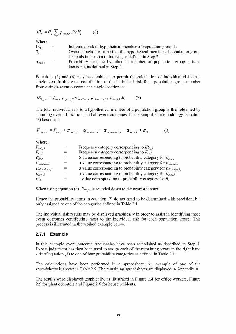
13
�=i
ikilockk FoFpIR .. ,,θ (6)
Where: IRk = Individual risk to hypothetical member of population group k. θk = Overall fraction of time that the hypothetical member of population group
k spends in the area of interest, as defined in Step 2. ploc,i,k = Probability that the hypothetical member of population group k is at
location i, as defined in Step 2. Equations (5) and (6) may be combined to permit the calculation of individual risks in a single step. In this case, contribution to the individual risk for a population group member from a single event outcome at a single location is:
kkilocjidirectionjweatherjifatjeokji ppppfIR θ..... ,,,,,,,,,, = (7) The total individual risk to a hypothetical member of a population group is then obtained by summing over all locations and all event outcomes. In the simplified methodology, equation (7) becomes:
kkilocjidirectionjweatherjifatjeokjIRi FF θααααα +++++= ,,,,,,,,,, (8) Where: FIRi,j,k = Frequency category corresponding to IRi,j,k Feo,j = Frequency category corresponding to Feo,j αfat,i,j = α value corresponding to probability category for pfat,i,j αweather,j = α value corresponding to probability category for pweather,j αdirection,i,j = α value corresponding to probability category for pdirection,i,j αloc,i,k = α value corresponding to probability category for ploc,i,k αθk = a value corresponding to probability category for θk When using equation (8), FIRi,j,k is rounded down to the nearest integer. Hence the probability terms in equation (7) do not need to be determined with precision, but only assigned to one of the categories defined in Table 2.1. The individual risk results may be displayed graphically in order to assist in identifying those event outcomes contributing most to the individual risk for each population group. This process is illustrated in the worked example below. 2.7.1 Example
In this example event outcome frequencies have been established as described in Step 4. Expert judgement has then been used to assign each of the remaining terms in the right hand side of equation (8) to one of four probability categories as defined in Table 2.1. The calculations have been performed in a spreadsheet. An example of one of the spreadsheets is shown in Table 2.9. The remaining spreadsheets are displayed in Appendix A. The results were displayed graphically, as illustrated in Figure 2.4 for office workers, Figure 2.5 for plant operators and Figure 2.6 for house residents.

14
Each figure may be thought of as a type of bar graph. The graph provides an indication of the event outcome contributing most to the individual risk. The higher up the chart an event outcome appears, the greater its individual risk contribution. In the case of office workers (Figure 2.4), event outcomes 2a/D5 and 2a/F2 are the most significant risk contributors. The graph can also provide an indication of where the individual is most at risk. This can be seen in Figure 2.5, which shows the completed individual risk graph for plant operators. Inspection of the various columns of the graph reveals that operators experience the greatest contribution to their individual risk during the time spent working on the plant and that the most significant individual risk contributors are event outcomes 1a/D5 and1a/F2. The shaded area at the top of the Figure 2.4 and Figure 2.5 indicates the region of unacceptable risk for workers, in excess of 10-3 per year [4]. Similarly, the shaded area in Figure 2.6 represents the region of unacceptable risk for members of the public, in excess of 10-4 per year [4]. Clearly, if any single event outcome appears in this area of the graph then the overall risk to individuals in that population group would be unacceptable. However, it should be noted that the converse is not true – if no event outcomes appeared in this section of the graph this would not necessarily indicate that the total of all of the individual risk contributions was in the tolerable region. In order to show that the overall individual risk is tolerable or broadly acceptable, it would be necessary to sum all of the individual risk contributions. An estimate of the total individual risk to the hypothetical member of a population group may be estimated using the expression:
.....10.10.10.10. 4,
5,
6,
7,,
−−−− +++= kEkFkGkHktot mmmmIR (9) Where: IRtot,k = Total individual risk to hypothetical member of population group k. mX,k = Number of event outcomes in category X for population group k. When using equation (9), the result is rounded up to the nearest significant figure (so that, for example, 2.4 x 10⁻⁶ becomes 3 x 10⁻⁶). It should be noted that the total individual risk estimated in this way is conservative, since the number of event outcomes in a category is multiplied by the upper limit of the frequency within that category. The total number of event outcomes in each category is shown in the right hand column of the graph. Hence, in the example, the total individual risk to office workers is:
676, 103)104()102( −−− ×=×+×=officetotIR per year
The total individual risk to plant operators is:
5765, 105)1014()104()104( −−−− ×=×+×+×=operatortotIR per year
Finally, the total individual risk to house residents is:
77, 103)103( −− ×=×=residenttotIR per year

15
For comparison purposes, equations (5) and (6) have been used to calculate individual risks explicitly, assuming release frequencies of 5 x10⁻⁴ per year for 5 mm leaks and 1.5 x 10⁻⁵ per year for pipe ruptures. The spreadsheets used are shown in Appendix A. The individual risks were then as follows: IRtot,office = 5.6 x 10⁻⁷ per year IRtot,operator = 4.9 x 10⁻⁶ per year IRtot,resident = 1.2 x 10⁻⁷ per year Hence the results obtained using the simplified method are, in this case, conservative by a factor of around 3-10, relative to the quantified result. The fully quantified approach indicated that the event outcomes contributing most to the risk were the same as those identified using the simplified method (i.e. – 2a/D5 and 2a/F2 for office workers and 1a/D5 and 1a/F2 for operators).

16
Table 2.9 Example Individual Risk Calculation Spreadsheet – Office Workers
Location: Office / Control Room (Indoor) Office Workers
Event Outcome
Frequency Category Impact pfat pweather pdirection ploc θk Factor
Individual Risk
Category
1a/D5 3 None 0 0
1a/F2 3 None 0 0
1b/D5 5 LD01 d e c e d 2 7
1b/F2 5 LD50 d e c e d 2 7
2a/D5 5 LD50 e e d e d 1 6
2a/F2 5 LD50 e d d e d 1 6
2b/D5 7 LD50 d d e e d 1 7
2b/F2 7 LD50 d e e e d 1 7

17
Figure 2.4 Example Individual Risk Graph – Office Workers
Category 0
>10-1 1
10-1 - 10-2 2
10-2 - 10-3 3
10-3 - 10-4 4
10-4 - 10-5 5
10-5 - 10-6 6 2a/D5 2
10-6 -10-7 2a/F2 7 1b/D5 4
<10-7 1b/F2 2b/D5 2b/F2 Office Plant Chlorine Building Housing Total No. Location

18
Figure 2.5 Example Individual Risk Graph – Plant Operators
Category 0
>10-1 1
10-1 - 10-2 2
10-2 - 10-3 3
10-3 - 10-4 4 0
10-4 - 10-5 5 1a/D5 1a/D5 4
10-5 - 10-6 1a/F2 1a/F2 6 2a/D5 1b/D5 2a/F2 4
10-6 -10-7 2a/D5 7 1b/D5 2b/F2 1b/F2 1b/D5 15
<10-7 1b/F2 2b/D5 1b/F2 2b/D5 2b/F2 2a/D5 2b/D5 2a/F2 2a/F2 2b/F2 Office Plant Chlorine Building Housing Total No. Location

19
Figure 2.6 Example Individual Risk Graph – House Residents
Category A
>10-1 B
10-1 - 10-2 C
10-2 - 10-3 D
10-3 - 10-4 E
10-4 - 10-5 F
10-5 - 10-6 G
10-6 -10-7 H 2a/F2 3
<10-7 2b/D5 2b/F2 Office Plant Chlorine Building Housing Total No. Location

20
3. RELATIONSHIP WITH THE RISK MATRIX
The process of constructing a risk matrix, where the consequence categories are expressed in terms of the number of fatalities, consists of the following steps: 1. Define probability and frequency categories for use in the study. 2. Define population groups of interest and their characteristics. 3. Define event outcomes of interest. 4. Estimate frequencies of event outcomes. 5. Estimate consequences of event outcomes. 6. Determine impacts of event outcomes at locations of interest. 7. Estimate numbers of fatalities and corresponding frequencies. 8. Plot frequency-number of fatality pairs on a matrix. Step 2 differs from the corresponding step in estimating individual risk in that the information required is the expected number of people at each location of interest at a given time. It may be necessary to differentiate between the population distributions occurring at different times (daytime and night-time, for example). Steps 3 to 6 inclusive are identical to those described for the estimation of individual risk. In Step 7 the expected number of fatalities may be estimated using:
jlocjifatji npn ,,,, .= (10) Where: ni,j = Expected number of fatalities at location i produced by event outcome
j. pfat,i,j = Probability of fatality at location i produced by event outcome j (as
before). nloc,j = Total number of people at location i (from population distribution). This expression does not differentiate between fatalities among different population groups. In the simplified methodology, equation (10) becomes:
jifatilicji nn ,,10.,,
α−= (11) The corresponding frequency with which this number of fatalities is expected to occur is given by:
itimejidirectionjweatherjeoji pppfnf ,,,,,, ...)( = (12) Where: f(ni,j) = Frequency with which the number of fatalities ni,j is expected to occur. feo,j = Frequency of event outcome j (as before). pweather,j = Probability of the weather conditions required to produce the event
outcome at j (from meteorological data, 1 for weather independent event outcomes, as before).

21
pdirection,i,j = Probability of event outcome j being directed at location i (related to the wind rose and cloud width for gas dispersion events, 1 for omni-directional events, as before).
ptime,i = Probability of the time of day (day, night, weekend etc.) for which the population at location i is nloc,i (1 if no distinction is made between different times of the day or week).
In the simplified methodology, equation (12) becomes:
itimejidirectionjweatherjeoji FnF ,,,,,, )( ααα +++= (13) Where: F(ni,j) = Frequency category corresponding to f(ni,j) Feo,j = Frequency category corresponding to feo,j αweather,j = α value corresponding to probability category for pweather,j αdirection,i,j = α value corresponding to probability category for pdirection,i,j αtime,i = α value corresponding to probability category for ptime,i When using equation (13), F(ni,j) is rounded down to the nearest integer. In the final step, the F(ni,j) – ni,j pairs are plotted on the matrix. Hence a significant amount of the information generated in estimating individual risk using the method described could, with a few additional operations, be used to generate a risk matrix. The information could be processed further to generate Potential Loss of Life (PLL) estimates, as follows:
�=ji
jiktot nIRPLL,
,, . (14)
Where: nk = number of people in population group k In deriving a set of f-n points, caution must be observed when dealing with omni-directional events, with adjacent populations, or populations lying in a similar direction from an event source. In the case of omni-directional events (such as a vapour cloud explosion or a BLEVE), the event outcome can affect several populations at once. This is illustrated in Figure 3.1.

22
Figure 3.1 Effect of Omni-Directional Event
Hazard range from event
Population A
Population B
Population CEvent
Hazard range from event
Population A
Population B
Population CEvent
Here, the same event can affect populations A, B and C simultaneously. This does not represent three f-n points but one, with three contributions to the value of n, one from each of the populations affected. It is also possible for a directional event (such as a gas plume or jet flame) to affect more than one population at once, if the populations are adjacent or lie in the same direction from the source. This is illustrated in Figure 3.2.

23
Figure 3.2 Effect of Adjacent Populations / Populations in Similar Direction
Population A
Population B
AdjacentPopulations
Population A
Population B
Populations inSimilar Direction
Source
Source
Population A
Population B
AdjacentPopulations
Population A
Population B
Populations inSimilar Direction
Source
Source
In the uppermost example in Figure 3.2, the adjacent populations A and B are simultaneously affected by the same event outcome. In the lower example, the populations are not adjacent but are in a similar direction from the source. Again, both populations are affected simultaneously. In both examples this results in not two f-n points but one, with two contributions to the value of n, one from each of the populations affected. In order to avoid double-counting due to these effects, it is suggested that: • Omni-directional events are highlighted at Step 3 and contributions to the number of
fatalities summed together at Step 7; and • Directional events that can effect more than one population at once are identified at
Step 6 and an appropriate summation of numbers of fatalities performed at Step 7. An example of an omni-directional event is considered in Appendix B.
3.1 EXAMPLE
Referring to the chlorine storage example used in the previous section, a population distribution was determined and is shown in Table 3.1.
Table 3.1 Example Population Distribution
Offices Plant Chlorine Building Housing
Number at location (day) 14 1 1 25
Number at location (night) 3 1 0 25

24
The numbers of personnel in each population group are displayed in Table. It is assumed that there are two teams of operators of four personnel each.
Table 3.2 Example Population Numbers
Population Group Number in Group, nkOffice workers 12
Plant operators 8
House residents 25
As a simplifying assumption, a 50:50 split has been assumed between day and night. It is further assumed that F2 weather only occurs at night. The event outcomes, event outcome frequencies and impact levels at locations of interest are as described previously. The various probabilities were again assigned to probability categories using expert judgement. This information has been combined within spreadsheets in order to obtain estimated numbers of fatalities using equation (11). F(ni,j) has been calculated using equation (13). Calculations were performed using a spreadsheet. As each f-n point was generated in the spreadsheet, it was assigned an identifier. The format of these identifiers is as follows:
EO/W/LOC/t Where: EO = Event outcome reference (1a, 2b etc.) W = Weather stability class / windspeed combination (D5 or F2) LOC = Location identifier (OFF for offices, PL for plant, CL for chlorine
building or HO for housing). t = Time of day (d for day, n for night). The identifiers were then placed in the appropriate cells in the risk matrix. Use of identifiers to indicate f-n points assists in the identification of which event outcome / population group combinations are significant contributors to societal risk. Note that populations of interest are well separated and lie in different directions from the source. An example of the spreadsheets is shown in Table 3.3. The remaining spreadsheets are contained in Appendix A. The resulting risk matrix is shown in Figure 3.3. The event outcomes contributing most significantly to the societal risk are those with the highest frequency in each consequence category. These are: • For 10<n≤30, 2a/D5/OFF/d (Event outcome 2a/D5 affecting people in the offices
during the day); • For 3<n≤10, 1b/D5/OFF/d (Event outcome 1b/D5 affecting people in the offices
during the day) and 2a/F2/HO/n (Event outcome 2a/F2 affecting people in the housing area during the night);
• For 1<n≤3, 2a/D5/OFF/n (Event outcome 2a/D5 affecting people in the offices during the night); and
• For n≤1, 1a/D5/CL/d (Event outcome 1a/D5 affecting people in the chlorine building during the day).

25
The event outcomes contributing most to individual risk were: • Event outcomes 2a/D5 and 2a/F2 in the case of office workers; • Event outcome 1a/D5 in the case of operators; and • Event outcome 2a/F2 in the case of house residents. Hence event outcomes 1a/D5, 2a/D5 and 2a/F2 make a significant contribution to both individual and societal risk. However, event outcome 1b/D5 contributes significantly to societal risk but not to individual risk. Equation (14) has been used to obtain an estimate of PLL: PLL = 4.4 x 10⁻⁴
26
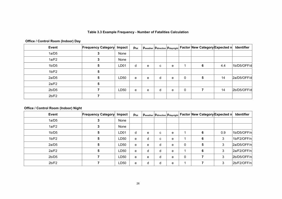
Table 3.3 Example Frequency - Number of Fatalities Calculation
Office / Control Room (Indoor) Day
Event Frequency Category Impact pfat pweather pdirection pdaynight Factor New CategoryExpected n Identifier
1a/D5 3 None
1a/F2 3 None
1b/D5 5 LD01 d e c e 1 6 4.4 1b/D5/OFF/d
1b/F2 5
2a/D5 5 LD50 e e d e 0 5 14 2a/D5/OFF/d
2a/F2 5
2b/D5 7 LD50 e e d e 0 7 14 2b/D5/OFF/d
2b/F2 7
Office / Control Room (Indoor) Night
Event Frequency Category Impact pfat pweather pdirection pdaynight Factor New CategoryExpected n Identifier
1a/D5 3 None
1a/F2 3 None
1b/D5 5 LD01 d e c e 1 6 0.9 1b/D5/OFF/n
1b/F2 5 LD50 e d c e 1 6 3 1b/F2/OFF/n
2a/D5 5 LD50 e e d e 0 5 3 2a/D5/OFF/n
2a/F2 5 LD50 e d d e 1 6 3 2a/F2/OFF/n
2b/D5 7 LD50 e e d e 0 7 3 2b/D5/OFF/n
2b/F2 7 LD50 e d d e 1 7 3 2b/F2/OFF/n

27
Figure 3.3 Example Risk Matrix
Frequency Category 7 6 5 4 3 2 1 0 >30 10<n≤30 2b/D5/OFF/d 2a/D5/OFF/d 3<n≤10 2b/D5/HO/d 1b/D5/OFF/d 2b/D5/HO/n 2a/F2/HO/n 2b/F2/HO/n
Number of
Fatalities 1<n≤3 2b/D5/OFF/n 1b/F2/OFF/n 2a/D5/OFF/n n 2b/F2/OFF/n 2a/F2/OFF/n n≤1 2b/D5/PL/d 1b/D5/OFF/n 2a/D5/PL/d 1a/D5/PL/d 1a/D5/CL/d 2b/D5/PL/n 1b/D5/PL/d 2a/D5/PL/n 1a/D5/PL/n 2b/F2/PL/n 1b/D5/PL/n 1b/D5/CL/d 1a/F2/PL/n 2b/D5/CL/d 1b/F2/PL/n 2a/D5/CL/d 2a/F2/PL/n

28
4. EFFECT OF RISK REDUCTION MEASURES
The method may be used to investigate the effect of introducing further measures to reduce risk at an establishment. The effect of implementing a new risk reduction measure may be to reduce the frequency of an event outcome (or event outcomes) or to reduce the consequence of an event outcome (or event outcomes), or both. The change in risk levels is determined by altering the frequency data or consequence data as required and re-estimating the risk. The change in risk can then be compared with the cost of implementing the measure, in order to determine whether or not the additional measure is reasonably practicable. It should be noted that the simplified nature of the method renders it relatively insensitive to small changes in either frequency or consequences. For example, use of the frequency categories as defined in Table 2.2 would mean that the method would be unable to measure the effect of changes in event outcome frequency of less than an order of magnitude. Similarly, Figure 4.1 illustrates a reduction in the hazard range of an event outcome following introduction of a risk reduction measure. However, since Population A is affected in both cases, the method would indicate no reduction in individual risk to the members of this group.
Figure 4.1 Example of Insensitivity to Reduction in Consequences
Before After
Source Source
Population A Population A
Before After
Source Source
Population A Population A
4.1 EXAMPLE
Referring to the chlorine storage example described in Section 2, it was determined that the event outcome 1a (isolated 5 mm leaks from chlorine pipework) contributed a significant proportion of the total individual risk to operators. The effect of reducing the frequency of this event outcome (for example, by using all-welded pipework) was therefore investigated. It was estimated that the introduction of such a measure would reduce the frequency of 5 mm leaks from pipework by an order of magnitude (although the rupture frequency would remain unchanged). The consequences of such events would remain as before. The revised event outcome frequency categories are therefore 4 and 6 for event outcomes 1a and 1b respectively. Re-estimating the individual risks and frequency-number of fatality data gives the revised individual risk graph for operators shown in Figure 4.2, and the revised risk matrix shown in Figure 4.3. The individual risks to office workers and house residents do not change significantly. Note that the effect of an order of magnitude reduction in the release frequency results in an order of magnitude reduction in the corresponding event outcome frequencies. In terms of the

29
individual risk graph in this example, this means that all of the 1a and 1b points are shifted one row downwards. In terms of the risk matrix, all of the 1a and 1b points are shifted one column to the left. Estimating the total individual risk using equation (8) gives: IRoperator = 9 x 10⁻⁶ per year Hence the individual risk to operators would be reduced by around a factor of 5 if this measure were to be introduced. The revised PLL value is as follows: PLL = 1.2 x 10⁻⁴ Hence the PLL has also reduced by around a factor of three to four. In order to determine whether or not this measure is reasonably practicable, it is necessary to compare the risk reduction that would be achieved with the cost of implementing the measure. One simple way of doing this is to calculate the Implied Cost of Avoiding a Fatality (ICAF). The ICAF is given by:
).( PLLLCICAF
∆= (15)
Where: C = Cost of implementing measure (£) L = Estimated lifetime of plant (years) ∆PLL = Change in PLL following implementation of the measure (fatalities per
year) ICAF values have been calculated for various implementation costs, assuming a plant lifetime of 20 years. The results are shown in Table 4.1.

30
Table 4.1 Example ICAF Values
Cost of Measure (£)
ICAF (£/fatality averted)
1,000 154,000
10,000 1,540,000
100,000 15,400,000 Hence at a cost of £1,000, the ICAF is significantly less than the value of a statistical fatality of £1 million discussed in Reference [HOLD], hence the measure would clearly be reasonably practicable. At a cost of £10,000, the ICAF is close to the value of a statistical fatality discussed in Reference [5], but not significantly greater. According to Reference [5], the factor for gross disproportion varies between 1 at the broadly acceptable boundary (of 1 x 10⁻⁶ /yr individual risk [4]) to 10 or more at the intolerable boundary (of 1 x 10⁻³ /yr individual risk for workers [4]). In this case the individual risk is estimated to be in the ‘Tolerable’ region, therefore the factor for gross disproportion could be taken to be around 3-5. Hence the cost would not be considered grossly disproportionate to the benefit and the measure would be reasonably practicable. At a cost of £100,000, the ICAF exceeds 15 times the value of a statistical fatality discussed in [5]. Since the individual risk is in the tolerable region, the cost in this case is clearly disproportionate to the benefits and the measure would not be considered reasonably practicable.

31
Figure 4.2 Example Revised Individual Risk Graph for Operators
Frequency Category
0
>10-1
1
10-1 – 10-2
2
10-2 - 10-3
3
10-3 – 10-4
4
10-4 - 10-5
5 0
10-5 – 10-6
6 2a/D5 1a/D5 2a/D5 1a/D5 7
10-6 -10-7 1a/F2 2a/F2 1a/F2
7 1b/D5 2b/F2 1b/D5 1b/D5 2b/D5 15
<10-7 1b/F2 1b/F2 1b/F2 2b/F2
2a/F2 2b/D5 2a/D5
2b/D5 2b/F2 2a/F2
Office Plant Chlorine Building Housing Total No.
Location

32
Figure 4.3 Example Revised Risk Matrix
Frequency
Category
7 6 5 4 3 2 1 0
>30
10<n≤30 2b/D5/OFF/d 2a/D5/OFF/d
3<n≤10 1b/D5/OFF/d 2a/F2/HO/n
2b/D5/HO/d
Number 2b/F2/HO/n
of 2b/D5/HO/n
Fatalities 1<n≤3 2b/D5/OFF/n 2a/F2/OFF/n 2a/D5/OFF/n
n 2b/F2/OFF/n
1b/F2/OFF/n
n≤1 2b/D5/PL/d 1b/D5/PL/d 2a/F2/PL/n 2a/D5/PL/d 1a/F2/PL/n 1a/D5/CL/d
2b/D5/PL/n 1b/D5/PL/n 1b/D5/CL/d 2a/D5/PL/n
2b/F2/PL/n 1b/F2/PL/n 2a/D5/CL/d
2b/D5/CL/d 1a/D5/PL/d
1b/D5/OFF/n 1a/D5/PL/n

33
5. SUMMARY AND CONCLUSIONS
The methodology presented in the previous sections is a development of the approach for calculating individual risk as outlined in the CCPS publication on LOPA [1], combined with elements of the procedure usually undertaken in order to construct a risk matrix. The method may be useful in the context of preparing a COMAH safety report, where use of a semi-quantified approach is justified. The method provides a simplified means of obtaining a conservative estimate of the individual risk to members of defined population groups. It can also be used to identify those event outcomes contributing most to the risk for each of the population groups specified. The method may be implemented within a spreadsheet. However, the effort involved in using the method increases rapidly as the numbers of event outcomes, population groups and hazardous material locations are increased. It is recommended that use of the method be considered when: • The number of event outcomes of interest is modest (50-100); • The hazardous materials on site are found at a few discrete locations (1-3); and • The number of population groups of interest is small (5 or less). Hence the method is likely to be of use at, for example, chlorine water treatment works or bulk LPG storage facilities in relatively sparsely populated areas. However, it may only be of limited use at more complex establishments in more densely populated areas. Several of the steps in the methodology are identical with the corresponding steps in the preparation of a risk matrix. It is possible to use the method to estimate individual risk and construct a risk matrix as a parallel activity. It has been observed that those events contributing most to individual risk are not necessarily the same as those events contributing most to societal risk. The method can be used in a comparative sense in order to judge the effectiveness of proposed risk reduction measures. However, owing to the simplified nature of the method, it is relatively insensitive to small changes in event frequencies or event consequences.

34
6. REFERENCES
1. Center for Chemical Process Safety (CCPS) 2001. ‘Layer of Protection Analysis – Simplified Process Risk Assessment’. American Institute of Chemical Engineers.
2. Health and Safety Executive 1999. ‘A guide to the Control of Major Accident Hazards Regulations 1999’. HSE Books, L111.
3. Middleton M L and Franks A P 2001. ‘Using Risk Matrices’. The Chemical Engineer, September 2001, p34-37.
4. Health and Safety Executive 2001. ‘Reducing risks, protecting people – HSE’s decision making process’. HSE Books.
5. HSE / HID (2002). ‘Guidance on ‘As Low As Reasonably Practicable’ (ALARP) Decisions in Control of Major Accident Hazards (COMAH)’. SPC/Permissioning/12, available at: http://www.hse.gov.uk/hid/spc/perm12/index.htm .
6. The Oil Industry International Exploration and Production Forum (E&P Forum), 1992. ‘Hydrocarbon Leak and Ignition Data Base’. Report No. 11.4/180.
7. Pape R P and Nussey C. “A Basic Approach for the Analysis of Risks from Major Toxic Hazards”. IChemE Symposium Series No. 93, p367-388.

35
APPENDIX A Chlorine Worked Example

36
A1. INTRODUCTION
The method comprises the following steps: 1. Define probability and frequency categories for use in the study. 2. Define population groups of interest and their characteristics. 3. Define event outcomes of interest. 4. Estimate frequencies of event outcomes. 5. Estimate consequences of event outcomes. 6. Determine impacts of event outcomes at locations of interest. 7. Estimate individual risk. Each of these steps has been applied to a hypothetical chlorine water treatment works in order to illustrate use of the method. The data used have been selected for the purposes of the example and are not based on any real sources or modelling.

37
A2. STEP 1: DEFINE PROBABILITY AND FREQUENCY CATEGORIES
Calculations are simplified by use of probability and frequency categories. These should be defined at the beginning of the study. The categories selected should be appropriate for the situation under consideration. The probability and frequency categories used in this example are displayed in Table A2.1 and Table A2.2 respectively.
Table A2.1 Probability Categories
Probability Category
a b c d e
Range p≤0.01 0.01<p≤0.03 0.03<p≤0.1 0.1<p≤0.3 0.3<p≤1
Value 0.01 0.03 0.1 0.3 1
-Log (Value), α 2 1.5 1 0.5 0
Each category represents a range of probabilities (the ‘Range’ shown in Table A2.1). This range is represented by the value corresponding to the maximum within that range (the ‘Value’ within Table A2.2). Associated with each category is a parameter, α, which is the negative of the logarithm (base 10) of the value representing that range. This is done to simplify calculations at a later stage, and ensure a conservative result.
Table A2.2 Frequency Categories
Category Frequency range (per year)
0 >10-1
1 10-1 to 10-2
2 10-2 to 10-3
3 10-3 to 10-4
4 10-4 to 10-5
5 10-5 to 10-6
6 10-6 to 10-7
7 <10-7
The frequency categories have deliberately been drawn very broadly so that the same categories could be applied to release frequencies, event outcome frequencies and individual risks if required.

38
A3. STEP 2: DEFINE POPULATION GROUPS
Consider the establishment displayed in Figure A3.1. The site is a water treatment works (much simplified) storing bulk chlorine in a building at one end of the site. The building also contains evaporators, supplied by liquid chlorine via pipework from the bulk tanks. There is an area of housing to the south-west of the site. The site control room is located within the office block at the western end of the site. The population groups of interest and their characteristics are given in Table A3.1.
Table A3.1 Example Population Groups
Proportion of time at location (ploc,i,k) Population Group
Office Plant Chlorine Building Housing
Overall Occupancy
θk
Office staff E d
Plant operators d e b d
Residents (off-site) e e
The ploc,i,k and θk parameters have been assigned probability categories by reference to Table A3.1. Therefore the values of these parameters do not need to be determined with great accuracy. θk represents the proportion of the year that the individual spends at the site. The ploc,i,k values describe where the individual spends their time while they are at the site.
Information concerning the various locations of interest is given in Table A3.2.
Figure A3.1 Example Establishment
1
2
3
4
Key1. Offices2. Plant3. Chlorine storage building4. Residential area
1
2
3
4
Key1. Offices2. Plant3. Chlorine storage building4. Residential area

39
Table A3.2 Example Location Information
Location: Office Plant Chlorine Building Housing
Type (Indoor or Outdoor) Indoor Outdoor Indoor Indoor
Distance to chlorine building (m) 200 150 0 750

40
A4. STEP 2: DEFINE EVENT OUTCOMES OF INTEREST
A HAZOP study for the hypothetical water treatment works in Figure A3.1 has identified the possibility of leaks of chlorine from the pipework carrying liquid chlorine from the bulk tanks to the evaporators (for the purposes of the example, flanged joints and gaskets have been included with the pipework). Releases may be small (5 mm equivalent hole diameter) or large (full bore rupture of the 25 mm diameter pipe). Furthermore, since the liquid lines are fitted with Automatic Shut-Off Valves (ASOVs) operating on detection of chlorine, a range of event outcomes are possible. This is illustrated in the event tree in Figure A4.1.
Figure A4.1 Example Event Tree
ASOV closes 2 minute release Y Leak N 20 minute release
Hence there are four outcomes of interest, as listed in Table A4.1.
Table A4.1 Example Outcomes of Interest
Identifier Description
1a 5 mm leak from pipework, 2 minute duration
1b 5 mm leak from pipework, 20 minute duration
2a Rupture of pipework, 2 minute duration
2b Rupture of pipework, 20 minute duration

41
A5. STEP 3: ESTIMATE FREQUENCIES OF EVENT OUTCOMES
Using expert judgement, the release frequencies have been assigned to the following categories: • Release 1 – 5 mm leak from pipework: Frequency Category, F5mm = 3 • Release 2 - Rupture of 25 mm pipe: Frequency Category, FRupture = 5 The event tree in Figure A4.1 has then been used to aid decisions regarding the assignment of event outcomes to frequency categories. Using conventional event tree logic, the frequency of the event outcomes would be given by:
failrelease pff .min20 = (1) and
)1.(min2 failrelease pff −= (2) Where f2min = Frequency of 2 minute release f20min = Frequency of 20 minute release pfail = Probability of ASOV failure of demand frelease = Frequency of release In the methodology these equations become:
failleaseFF α+= Remin20 (3) and
successleaseFF α+= Remin2 (4) Where F2min = Frequency category corresponding to f2min F20min = Frequency category corresponding to f20min αfail = a value corresponding to probability category for pfail αsuccess = a value corresponding to probability category for (1-pfail) It is estimated that the probability of failure on demand of the ASOV is in probability category a, giving a value for αfail of 2. The probability of the ASOV working successfully is therefore close to unity, in probability category e, giving a value for αsuccess of 0. Using equations (3) and (4), the frequency categories for each of the outcomes of interest in Table A4.1 may now be obtained.
successmma FF α+= 51 3031 =+=aF

42
failmmb FF α+= 51
5231 =+=bF
successRupturea FF α+=2
5052 =+=aF
failRuptureb FF α+=2
7252 =+=bF The frequency categories for the outcomes of interest are summarised in Table A5.1.
Table A5.1 Example – Assigned Event Outcome Frequency Categories
Event Outcome Description Event Outcome
Frequency Category
1a 5 mm leak from pipework, 2 minute duration 3
1b 5 mm leak from pipework, 20 minute duration 5
2a Rupture of pipework, 2 minute duration 5
2b Rupture of pipework, 20 minute duration 7

43
A6. STEP 4: ESTIMATE CONSEQUENCES OF EVENTS
The hazard ranges shown in Table A6.1 have been specified for the purposes of the example. Two weather stability class – wind speed combinations have been considered: D5 and F2.
Table A6.1 Example Consequence Analysis Results
Hazard Ranges (m)
People Outdoors People IndoorsCase
LD50 LD01 LD50 LD01
1a/D5 60 160 30 90
1a/F2 180 290 80 130
1b/D5 220 300 160 240
1b/F2 350 550 210 360
2a/D5 640 800 310 480
2a/F2 920 1200 610 790
2b/D5 850 1150 570 810
2b/F2 1050 1400 910 1200

44
A7. STEP 5: DETERMINE THE IMPACTS OF EVENT OUTCOMES AT LOCATIONS OF INTEREST
The distances between the locations of interest and the chlorine building (as given in Table A3.2) were compared with the appropriate hazard ranges in Table A6.1. A table showing the impact level reached at the locations of interest for each of the event outcomes was then prepared and is shown in Table A7.1. Note that, for the offices, houses and chlorine building the hazard ranges for people indoors were applied. For the plant area, the hazard ranges for people outdoors were applied.
Table A7.1 Example Impact Levels at Locations of Interest
Location of Interest Event Outcome
Offices Plant Chlorine Building Housing
1a/D5 None LD01 LD50 None
1a/F2 None LD50 LD50 None
1b/D5 LD01 LD50 LD50 None
1b/F2 LD50 LD50 LD50 None
2a/D5 LD50 LD50 LD50 None
2a/F2 LD50 LD50 LD50 LD01
2b/D5 LD50 LD50 LD50 LD01
2b/F2 LD50 LD50 LD50 LD01

45
A8. STEP 6: ESTIMATE INDIVIDUAL RISK
The next step in the method involves the calculation of the individual risk to the members of the population groups of interest. This has been performed using equations (8) and (9) of the main report. In this example event outcome frequencies have been established as described in Step 4. Expert judgement has then been used to assign each of the remaining terms in the right hand side of equation (8) to one of four probability categories as defined in Table A2.1. The calculations have been performed in a spreadsheet. The outputs are shown in Tables A8.1 to A8.3. The results have then been displayed in graphical form as shown in Figures A8.1 to A8.3. Hence, the total individual risk to office workers is:
676, 103)104()102( −−− ×=×+×=officetotIR per year
The total individual risk to plant operators is:
5765, 105)1014()104()104( −−−− ×=×+×+×=operatortotIR per year
Finally, the total individual risk to house residents is:
77, 103)103( −− ×=×=residenttotIR per year

46
Table A8.1 Simplified Individual Risk Calculation – Office Workers
Location Event Frequency Category Impact pfat,i,j pweather,j pdirection,i,j ploc,i,k θk Factor Individual
Risk Category
Offices (Indoor) 1a/D5 3 None
1a/F2 3 None
1b/D5 5 LD01 d e c e d 2 7
1b/F2 5 LD50 d e c e d 2 7
2a/D5 5 LD50 e e d e d 1 6
2a/F2 5 LD50 e d d e d 1 6
2b/D5 7 LD50 d d e e d 1 7
2b/F2 7 LD50 d e e e d 1 7

47
Table A8.2 Simplified Individual Risk Calculation - Operators
Location Event Frequency Category Impact pfat,i,j pweather,j pdirection,i,j ploc,i,k θk Factor Individual
Risk Category Offices (Indoor) 1a/D5 3 None
1a/F2 3 None 1b/D5 5 LD01 d e c d d 2 7 1b/F2 5 LD50 d e c d d 2 7 2a/D5 5 LD50 e e d d d 1 6 2a/F2 5 LD50 e d d d d 2 7 2b/D5 7 LD50 d d e d d 2 7 2b/F2 7 LD50 d e e d d 1 7
Plant (Outdoor) 1a/D5 3 LD01 d e c e d 2 5 1a/F2 3 LD50 e d c e d 2 5 1b/D5 5 LD50 e e c e d 1 6 1b/F2 5 LD50 e d c e d 2 7 2a/D5 5 LD50 e e d e d 1 6 2a/F2 5 LD50 e d d e d 1 6 2b/D5 7 LD50 e e d e d 1 7 2b/F2 7 LD50 e d d e d 1 7
1a/D5 3 LD50 e e e b d 2 5 1a/F2 3 LD50 e d e b d 2 5 1b/D5 5 LD50 e e e b d 2 7 1b/F2 5 LD50 e d e b d 2 7 2a/D5 5 LD50 e e e b d 2 7 2a/F2 5 LD50 e d e b d 2 7 2b/D5 7 LD50 e e e b d 2 7
Chlorine Building (Indoor)
2b/F2 7 LD50 e d e b d 2 7

48
Table A8.3 Simplified Individual Risk Calculation – House Residents
Location Event Frequency Category Impact pfat,i,j pweather,j pdirection,i,j ploc,i,k θk Factor Individual Risk Category
Housing (Indoor) 1a/D5 3 None
1a/F2 3 None
1b/D5 5 None
1b/F2 5 None
2a/D5 5 None
2a/F2 5 LD01 d d d d d 2 7
2b/D5 7 LD01 d e d d d 2 7
2b/F2 7 LD01 d d d d d 2 7

49
Figure A8.1 Individual Risk Graph – Office Workers
Category
0
>10-1
1
10-1 - 10-2
2
10-2 - 10-3
3
10-3 - 10-4
4
10-4 - 10-5
5
10-5 - 10-6
6 2a/D5 2
10-6 -10-7 2a/F2
7 1b/D5 4
<10-7 1b/F2
2b/D5
2b/F2
Office Plant Chlorine Building Housing Total No.
Location

50
Figure A8.2 Individual Risk Graph - Operators
Category
0
>10-1
1
10-1 - 10-2
2
10-2 – 10-3
3
10-3 - 10-4
4
10-4 - 10-5
5 1a/D5 1a/D5 4
10-5 - 10-6 1a/F2 1a/F2
6 2a/D5 1b/D5 2a/F2 4
10-6 -10-7 2a/D5
7 1b/D5 2b/F2 1b/F2 1b/D5 2b/D5 14
<10-7 1b/F2 2b/D5 1b/F2 2b/F2
2a/F2 2b/F2 2a/D5
2b/D5 2a/F2
Office Plant Chlorine Building Housing Total No.
Location

51
Figure A8.3 Individual Risk Graph – House Residents
Category
0
>10-1
1
10-1 – 10-2
2
10-2 - 10-3
3
10-3 – 10-4
4
10-4 - 10-5
5
10-5 – 10-6
6
10-6 -10-7
7 3
<10-7 2a/F2
2b/D5
2b/F2
Office Plant Chlorine Building Housing Total No.
Location

52
For comparison purposes, equation (7) of the main report has been used to calculate individual risks explicitly, assuming release frequencies of 5 x10⁻⁴ per year for 5 mm leaks and 1.5 x 10⁻⁵ per year for pipe ruptures. An ASOV failure on demand probability of 0.01 was also assumed. The calculations are shown in the spreadsheet outputs in Tables A8.4 to A8.6, which also show the other probability values used. The individual risks were then as follows: IRtot,office = 5.6 x 10⁻⁷ per year IRtot,operator = 4.9 x 10⁻⁶ per year IRtot,resident = 1.2 x 10⁻⁷ per year

53
Table A8.4 Quantified Individual Risk Calculation – Office Workers
Location Event Frequency Impact pfat,i,j pweather,j pdirection,i,j ploc,i,k θk Individual Risk
Offices 1a/D5 5.00E-04 None
(Indoor) 1a/F2 5.00E-04 None
1b/D5 5.00E-06 LD01 0.25 0.85 0.1 1 0.23 2.44E-08
1b/F2 5.00E-06 LD50 0.75 0.15 0.1 1 0.23 1.29E-08
2a/D5 1.50E-05 LD50 0.75 0.85 0.2 1 0.23 4.40E-07
2a/F2 1.50E-05 LD50 0.75 0.15 0.2 1 0.23 7.76E-08
2b/D5 1.50E-07 LD50 0.75 0.85 0.25 1 0.23 5.50E-09
2b/F2 1.50E-07 LD50 0.75 0.15 0.25 1 0.23 9.70E-10
Total 5.61E-07

54
Table A8.5 Quantified Individual Risk Calculation - Operators
Location Event Frequency Impact pfat,i,j pweather,j pdirection,i,j ploc,i,k θk Individual Risk Offices 1a/D5 5.00E-04 None (Indoor) 1a/F2 5.00E-04 None
1b/D5 5.00E-06 LD01 0.25 0.85 0.1 0.3 0.23 7.33E-09 1b/F2 5.00E-06 LD50 0.75 0.15 0.1 0.3 0.23 3.88E-09 2a/D5 1.50E-05 LD50 0.75 0.85 0.2 0.3 0.23 1.32E-07 2a/F2 1.50E-05 LD50 0.75 0.15 0.2 0.3 0.23 2.33E-08 2b/D5 1.50E-07 LD50 0.75 0.85 0.25 0.3 0.23 1.65E-09 2b/F2 1.50E-07 LD50 0.75 0.15 0.25 0.3 0.23 2.91E-10
Plant 1a/D5 5.00E-04 LD01 0.25 0.85 0.1 0.68 0.23 1.66E-06 (Outdoor) 1a/F2 5.00E-04 LD50 0.75 0.15 0.1 0.68 0.23 8.80E-07
1b/D5 5.00E-06 LD50 0.75 0.85 0.1 0.68 0.23 4.99E-08 1b/F2 5.00E-06 LD50 0.75 0.15 0.1 0.68 0.23 8.80E-09 2a/D5 1.50E-05 LD50 0.75 0.85 0.2 0.68 0.23 2.99E-07 2a/F2 1.50E-05 LD50 0.75 0.15 0.2 0.68 0.23 5.28E-08 2b/D5 1.50E-07 LD50 0.75 0.85 0.25 0.68 0.23 3.74E-09 2b/F2 1.50E-07 LD50 0.75 0.15 0.25 0.68 0.23 6.60E-10
Chlorine Building 1a/D5 5.00E-04 LD50 0.75 0.85 1 0.02 0.23 1.47E-06 (Indoor) 1a/F2 5.00E-04 LD50 0.75 0.15 1 0.02 0.23 2.59E-07
1b/D5 5.00E-06 LD50 0.75 0.85 1 0.02 0.23 1.47E-08 1b/F2 5.00E-06 LD50 0.75 0.15 1 0.02 0.23 2.59E-09 2a/D5 1.50E-05 LD50 0.75 0.85 1 0.02 0.23 4.40E-08 2a/F2 1.50E-05 LD50 0.75 0.15 1 0.02 0.23 7.76E-09 2b/D5 1.50E-07 LD50 0.75 0.85 1 0.02 0.23 4.40E-10 2b/F2 1.50E-07 LD50 0.75 0.15 1 0.02 0.23 7.76E-11 Total 4.92E-06

55
Table A8.6 Quantified Individual Risk – House Residents
Location Event Frequency Impact pfat,i,j pweather,j pdirection,i,j ploc,i,k θk Individual
Risk
Housing 1a/D5 5.00E-04 None 0.00E+00
(Indoor) 1a/F2 5.00E-04 None 0.00E+00
1b/D5 5.00E-06 None 0.00E+00
1b/F2 5.00E-06 None 0.00E+00
2a/D5 1.50E-05 None 0.00E+00
2a/F2 1.50E-05 LD01 0.25 0.15 0.2 1 1 1.13E-07
2b/D5 1.50E-07 LD01 0.25 0.85 0.25 1 1 7.97E-09
2b/F2 1.50E-07 LD01 0.25 0.15 0.25 1 1 1.41E-09
Total 1.22E-07
56
A9. RISK MATRIX
For comparison purposes, a risk matrix has also been prepared for the same example. The process of constructing a risk matrix, where the consequence categories are expressed in terms of the number of fatalities, consists of the following steps: 1. Define probability and frequency categories for use in the study. 2. Define population groups of interest and their characteristics. 3. Define event outcomes of interest. 4. Estimate frequencies of event outcomes. 5. Estimate consequences of event outcomes. 6. Determine impacts of event outcomes at locations of interest. 7. Estimate numbers of fatalities and corresponding frequencies. 8. Plot frequency-number of fatality pairs on a matrix. Step 2 differs from the corresponding step in estimating individual risk in that the information required is the expected number of people at each location of interest at a given time. It may be necessary to differentiate between the population distributions occurring at different times (daytime and night-time, for example). Steps 3 to 6 inclusive are identical to those described for the estimation of individual risk. In Step 7 the expected number of fatalities may be estimated using equation (11) of the main report. The corresponding frequency category within which this number of fatalities is expected to occur is given by equation (13). In the final step, the F(ni,j) – ni,j pairs are plotted on the matrix. The information can be processed further to generate Potential Loss of Life (PLL) estimates, using equation (14) of the main report. A population distribution was determined and is shown in Table A9.1.
Table A9.1 Example Population Distribution
Offices Plant Chlorine Building Housing
Number at location (day) 14 1 1 25
Number at location (night) 3 1 0 25 The numbers of personnel in each population group are displayed in Table. It is assumed that there are two teams of operators of four personnel each.

57
Table 9.2 Example Population Numbers
Population Group Number in Group, nkOffice workers 12
Plant operators 8
House residents 25
As a simplifying assumption, a 50:50 split has been assumed between day and night. It is further assumed that F2 weather only occurs at night. The event outcomes, event outcome frequencies and impact levels at locations of interest are as described previously. The various probabilities were again assigned to probability categories using expert judgement. This information has been combined within spreadsheets in order to obtain estimated numbers of fatalities using equation (11). F(ni,j) has been calculated using equation (13). The calculations are displayed in the spreadsheet shown in Table A9.3. As each f-n point was generated in the spreadsheet, it was assigned an identifier. The identifiers were then placed in the appropriate cells in the risk matrix, as shown in Figure A9.1. Equation (14) has been used to obtain estimates of PLL: PLL = 4.4 x 10⁻⁴

58
Table A9.3 Calculation of f-n Data
Location / Time of Day Event Frequency Category Impact pfat,i,j pweather,j pdirection,i,j ptime,i Factor New Frequency Category Expected n Identifier
Offices/ Day 1a/D5 3 None 1a/F2 3 None 1b/D5 5 LD01 d e c e 1 6 4.4 1b/D5/OFF/d 1b/F2 5 2a/D5 5 LD50 e e d e 0 5 14 2a/D5/OFF/d 2a/F2 5 2b/D5 7 LD50 e e d e 0 7 14 2b/D5/OFF/d 2b/F2 7
Offices / Night 1a/D5 3 None 1a/F2 3 None 1b/D5 5 LD01 d e c e 1 6 0.9 1b/D5/OFF/n 1b/F2 5 LD50 e d c e 1 6 3 1b/F2/OFF/n 2a/D5 5 LD50 e e d e 0 5 3 2a/D5/OFF/n 2a/F2 5 LD50 e d d e 1 6 3 2a/F2/OFF/n 2b/D5 7 LD50 e e d e 0 7 3 2b/D5/OFF/n 2b/F2 7 LD50 e d d e 1 7 3 2b/F2/OFF/n
Plant / Day 1a/D5 3 LD01 d e c e 1 4 0.3 1a/D5/PL/d 1a/F2 3 1b/D5 5 LD50 e e c e 1 6 1 1b/D5/PL/d 1b/F2 5 2a/D5 5 LD50 e e d e 0 5 1 2a/D5/PL/d 2a/F2 5 2b/D5 7 LD50 e e d e 0 7 1 2b/D5/PL/d 2b/F2 7

59
Table A9.3 Calculation of f-n Data (continued)
Location / Time of Day Event Frequency Category Impact pfat,i,j pweather,j pdirection,i,j ptime,i Factor New Frequency Category Expected n Identifier
Plant / Night 1a/D5 3 LD01 d e c e 1 4 0.3 1a/D5/PL/n 1a/F2 3 LD50 e d c e 1 4 1 1a/F2/PL/n 1b/D5 5 LD50 e e c e 1 6 1 1b/D5/PL/n 1b/F2 5 LD50 e d c e 1 6 1 1b/F2/PL/n 2a/D5 5 LD50 e e d e 0 5 1 2a/D5/PL/n 2a/F2 5 LD50 e d d e 1 6 1 2a/F2/PL/n 2b/D5 7 LD50 e e d e 0 7 1 2b/D5/PL/n 2b/F2 7 LD50 e d d e 1 7 1 2b/F2/PL/n
Chlorine Building / 1a/D5 3 LD50 e e e e 0 3 1 1a/D5/CL/d
Day 1a/F2 3 1b/D5 5 LD50 e e e e 0 5 1 1b/D5/CL/d 1b/F2 5 2a/D5 5 LD50 e e e e 0 5 1 2a/D5/CL/d 2a/F2 5 2b/D5 7 LD50 e e e e 0 7 1 2b/D5/CL/d 2b/F2 7

60
Table A9.3 Calculation of f-n Data (continued)
Location / Time of Day Event Frequency Category Impact pfat,i,j pweather,j pdirection,i,j ptime,i Factor New Frequency Category Expected n Identifier
Chlorine Building / 1a/D5 3 LD50
Night 1a/F2 3 LD50 1b/D5 5 LD50 1b/F2 5 LD50 2a/D5 5 LD50 2a/F2 5 LD50 2b/D5 7 LD50 2b/F2 7 LD50 e d e e 0 7 0
Housing / Day 1a/D5 3 None 1a/F2 3 None 1b/D5 5 None 1b/F2 5 None 2a/D5 5 None 2a/F2 5 2b/D5 7 LD01 d e d e 0 7 7.9 2b/D5/HO/d 2b/F2 7
Housing / Night 1a/D5 3 None 1a/F2 3 None 1b/D5 5 None 1b/F2 5 None 2a/D5 5 None 2a/F2 5 LD01 d d d e 1 6 7.9 2a/F2/HO/n 2b/D5 7 LD01 d e d e 0 7 7.9 2b/D5/HO/n 2b/F2 7 LD01 d d d e 1 7 7.9 2b/F2/HO/n

61
Figure A6.1 Risk Matrix
Frequency
Category
7 6 5 4 3 2 1 0
>30
10<n≤30 2b/D5/OFF/d 2a/D5/OFF/d
3<n≤10 2b/D5/HO/d 1b/D5/OFF/d
2b/D5/HO/n 2a/F2/HO/n
Number 2b/F2/HO/n
of 1<n≤3 2b/D5/OFF/n 1b/F2/OFF/n 2a/D5/OFF/n
Fatalities 2b/F2/OFF/n 2a/F2/OFF/n
n≤1 2b/D5/PL/d 1b/D5/OFF/n 2a/D5/PL/d 1a/D5/PL/d 1a/D5/CL/d
2b/D5/PL/n 1b/D5/PL/d 2a/D5/PL/n 1a/D5/PL/n
2b/F2/PL/n 1b/D5/PL/n 1b/D5/CL/d 1a/F2/PL/n
2b/D5/CL/d 1b/F2/PL/n 2a/D5/CL/d
2a/F2/PL/n

62
A10. RISK REDUCTION
It was determined that the event outcome 1a (isolated 5 mm leaks from chlorine pipework) contributed a significant proportion of the total individual risk to operators. The effect of reducing the frequency of this event outcome (for example, by using all-welded pipework) was therefore investigated. It was estimated that the introduction of such a measure would reduce the frequency of 5 mm leaks from pipework by an order of magnitude (although the rupture frequency would remain unchanged). The consequences of such events would remain as before. The revised event outcome frequency categories are therefore 4 and 6 for event outcomes 1a and 1b respectively. Re-estimating the individual risks and frequency-number of fatality data gives the revised spreadsheets shown in Tables A10.2 to A10.5, the revised individual risk graph for operators as shown in Figure A10.1 and the revised risk matrix shown in Figure A10.2. The individual risks to office workers and house residents do not change significantly. The revised risks have been calculated in a spreadsheet. Note that the effect of an order of magnitude reduction in the release frequency results in an order of magnitude reduction in the corresponding event outcome frequencies. In terms of the individual risk graph in this example, this means that all of the 1a and 1b points are shifted one row downwards. In terms of the risk matrix, all of the 1a and 1b points are shifted one column to the left. Estimating the total individual risk using equation (8) gives: IRoperator = 9 x 10⁻⁶ per year Hence the individual risk to operators would be reduced by around a factor of 5 if this measure were to be introduced. The revised PLL value is as follows: PLL = 1.2 x 10⁻⁴ Hence the PLL has also reduced by around a factor of three to four. In order to determine whether or not this measure is reasonably practicable, it is necessary to compare the risk reduction that would be achieved with the cost of implementing the measure. One simple way of doing this is to calculate the Implied Cost of Avoiding a Fatality (ICAF). The ICAF is obtained using equation (15) of the main report. ICAF values have been calculated for various implementation costs, assuming a plant lifetime of 20 years. The results are shown in Table A10.1.
Table A10.1 Example ICAF Values
Cost of Measure (£)
ICAF (£/fatality averted)
1,000 154,000
10,000 1,540,000
100,000 15,400,000

63
Hence at a cost of £1,000, the ICAF is significantly less than the value of a statistical fatality of £1 million discussed in Reference [5], hence the measure would clearly be reasonably practicable. At a cost of £10,000, the ICAF is close to the value of a statistical fatality discussed in Reference [1], but not significantly greater. According to Reference [1], the factor for gross disproportion varies between 1 at the broadly acceptable boundary (of 1 x 10⁻⁶ /yr individual risk [2]) to 10 or more at the intolerable boundary (of 1 x 10⁻³ /yr individual risk for workers [2]). In this case the individual risk is estimated to be in the ‘Tolerable’ region, therefore the factor for gross disproportion could be taken to be around 3-5. Hence the cost would not be considered grossly disproportionate to the benefit and the measure would be reasonably practicable. At a cost of £100,000, the ICAF exceeds 15 times the value of a statistical fatality discussed in [1] Since the individual risk is in the tolerable region, the cost in this case is clearly disproportionate to the benefits and the measure would not be considered reasonably practicable.

64
Table A10.2 Revised Individual Risk – Office Workers
Location Event Frequency Category Impact pfat,i,j pweather,j pdirection,i,j ploc,i,k θk Factor
Individual Risk
Category
Offices 1a/D5 4 None
(Indoor) 1a/F2 4 None
1b/D5 6 LD01 d e c e d 2 7
1b/F2 6 LD50 d e c e d 2 7
2a/D5 5 LD50 e e d e d 1 6
2a/F2 5 LD50 e d d e d 1 6
2b/D5 7 LD50 d d e e d 1 7
2b/F2 7 LD50 d e e e d 1 7

65
Table A10.3 Revised Individual Risk - Operators
Location Event Frequency Category Impact pfat,i,j pweather,j pdirection,i,j ploc,i,k θk Factor Individual Risk
Category Offices (Indoor) 1a/D5 4 None 0 0
1a/F2 4 None 0 0 1b/D5 6 LD01 d e c d d 2 7 1b/F2 6 LD50 d e c d d 2 7 2a/D5 5 LD50 e e d d d 1 6 2a/F2 5 LD50 e d d d d 2 7 2b/D5 7 LD50 d d e d d 2 7 2b/F2 7 LD50 d e e d d 1 7
Plant (Outdoor) 1a/D5 4 LD01 d e c e d 2 6 1a/F2 4 LD50 e d c e d 2 6 1b/D5 6 LD50 e e c e d 1 7 1b/F2 6 LD50 e d c e d 2 7 2a/D5 5 LD50 e e d e d 1 6 2a/F2 5 LD50 e d d e d 1 6 2b/D5 7 LD50 e e d e d 1 7 2b/F2 7 LD50 e d d e d 1 7
Chlorine Building 1a/D5 4 LD50 e e e b d 2 6 (Indoor) 1a/F2 4 LD50 e d e b d 2 6
1b/D5 6 LD50 e e e b d 2 7 1b/F2 6 LD50 e d e b d 2 7 2a/D5 5 LD50 e e e b d 2 7 2a/F2 5 LD50 e d e b d 2 7 2b/D5 7 LD50 e e e b d 2 7 2b/F2 7 LD50 e d e b d 2 7

66
Table A10.4 Revised Individual Risk – House Residents
Location Event Freq. Cat Impact pfat,i,j pweather,j pdirection,i,j ploc,i,k θk Factor Individual Risk Category
Housing (Indoor) 1a/D5 4 None
1a/F2 4 None
1b/D5 6 None
1b/F2 6 None
2a/D5 5 None
2a/F2 5 LD01 d d d d d 2 7
2b/D5 7 LD01 d e d d d 2 7
2b/F2 7 LD01 d d d d d 2 7

67
Table A10.5 Revised Calculation of f-n Data
Location / Time of Day Event Frequency
Category Impact pfat,i,j pweather,j pdirection,i,j ptime,i Factor New Frequency Category
Expected n Identifier
1a/D5 4 None 1a/F2 4 None 1b/D5 6 LD01 d e c e 1 7 4.4 1b/D5/OFF/d 1b/F2 6 2a/D5 5 LD50 e e d e 0 5 14 2a/D5/OFF/d 2a/F2 5 2b/D5 7 LD50 e e d e 0 7 14 2b/D5/OFF/d
Offices / Day
2b/F2 7 1a/D5 4 None 1a/F2 4 None 1b/D5 6 LD01 d e c e 1 7 0.9 1b/D5/OFF/n 1b/F2 6 LD50 e d c e 1 7 3 1b/F2/OFF/n 2a/D5 5 LD50 e e d e 0 5 3 2a/D5/OFF/n 2a/F2 5 LD50 e d d e 1 6 3 2a/F2/OFF/n 2b/D5 7 LD50 e e d e 0 7 3 2b/D5/OFF/n
Offices / Night
2b/F2 7 LD50 e d d e 1 7 3 2b/F2/OFF/n 1a/D5 4 LD01 d e c e 1 5 0.3 1a/D5/PL/d 1a/F2 4 1b/D5 6 LD50 e e c e 1 7 1 1b/D5/PL/d 1b/F2 6 2a/D5 5 LD50 e e d e 0 5 1 2a/D5/PL/d 2a/F2 5 2b/D5 7 LD50 e e d e 0 7 1 2b/D5/PL/d
Plant / Day
2b/F2 7

68
Table A10.5 Revised Calculation of f-n Data (continued)
Location / Time of Day Event Frequency
Category Impact pfat,i,j pweather,j pdirection,i,j ptime,i Factor New Frequency Category
Expected n Identifier
1a/D5 4 LD01 d e c e 1 5 0.3 1a/D5/PL/n 1a/F2 4 LD50 e d c e 1 5 1 1a/F2/PL/n 1b/D5 6 LD50 e e c e 1 7 1 1b/D5/PL/n 1b/F2 6 LD50 e d c e 1 7 1 1b/F2/PL/n 2a/D5 5 LD50 e e d e 0 5 1 2a/D5/PL/n 2a/F2 5 LD50 e d d e 1 6 1 2a/F2/PL/n 2b/D5 7 LD50 e e d e 0 7 1 2b/D5/PL/n
Plant / Night
2b/F2 7 LD50 e d d e 1 7 1 2b/F2/PL/n 1a/D5 4 LD50 e e e e 0 4 1 1a/D5/CL/d 1a/F2 4 1b/D5 6 LD50 e e e e 0 6 1 1b/D5/CL/d 1b/F2 6 2a/D5 5 LD50 e e e e 0 5 1 2a/D5/CL/d 2a/F2 5 2b/D5 7 LD50 e e e e 0 7 1 2b/D5/CL/d
Chlorine Building /
Day
2b/F2 7 1a/D5 4 LD50 e e e e 0 4 0 1a/F2 4 LD50 e d e e 0 4 0 1b/D5 6 LD50 e e e e 0 6 0 1b/F2 6 LD50 e d e e 0 6 0 2a/D5 5 LD50 e e e e 0 5 0 2a/F2 5 LD50 e d e e 0 5 0 2b/D5 7 LD50 e e e e 0 7 0
Chlorine Building /
Night
2b/F2 7 LD50 e d e e 0 7 0

69
Table A10.5 Revised Calculation of f-n Data (continued)
Location / Time of Day Event Frequency
Category Impact pfat,i,j pweather,j pdirection,i,j ptime,i Factor New Frequency Category
Expected n Identifier
1a/D5 4 None
1a/F2 4 None
1b/D5 6 None
1b/F2 6 None
2a/D5 5 None
2a/F2 5
2b/D5 7 LD01 d e d e 0 7 7.9 2b/D5/HO/d
Housing / Day
2b/F2 7
1a/D5 4 None
1a/F2 4 None
1b/D5 6 None
1b/F2 6 None
2a/D5 5 None
2a/F2 5 LD01 d d d e 1 6 7.9 2a/F2/HO/n
2b/D5 7 LD01 d e d e 0 7 7.9 2b/D5/HO/n
Housing / Night
2b/F2 7 LD01 d d d e 1 7 7.9 2b/F2/HO/n

70
Figure A10.1 Revised Individual Risk Graph for Operators
Frequency Category
0 >10-1
1 10-1 - 10-2
2 10-2 - 10-3
3 10-3 - 10-4
4 10-4 - 10-5
5 10-5 - 10-6
6 2a/D5 1a/D5 2a/F2 1a/D5 7 10-6 -10-7 2a/D5 1a/F2 1a/F2
7 1b/D5 2b/F2 1b/F2 1b/D5 2b/D5 15 <10-7 1b/F2 2b/D5 1b/F2 2b/F2
2a/F2 2b/F2 2a/D5 2b/D5 1b/D5 2a/F2 Office Plant Chlorine Building Housing Total No. Location

71
Figure A10.2 Revised Risk Matrix
Frequency
Category
7 6 5 4 3 2 1 0
>30
10<n≤30 2b/D5/OFF/d 2a/D5/OFF/d
3<n≤10 1b/D5/OFF/d 2a/F2/HO/n
2b/D5/HO/d
2b/F2/HO/n
Number 2b/D5/HO/n
of 1<n≤3 2b/D5/OFF/n 2a/F2/OFF/n 2a/D5/OFF/n
Fatalities 2b/F2/OFF/n
1b/F2/OFF/n
N≤1 2b/D5/PL/d 1b/D5/PL/d 2a/F2/PL/n 2a/D5/PL/d 1a/F2/PL/n 1a/D5/CL/d
2b/D5/PL/n 1b/D5/PL/n 1b/D5/CL/d 2a/D5/PL/n
2b/F2/PL/n 1b/F2/PL/n 2a/D5/CL/d
2b/D5/CL/d 1a/D5/PL/d
1b/D5/OFF/n 1a/D5/PL/n

72
A11. REFERENCES
1. HSE / HID (2002). ‘Guidance on ‘As Low As Reasonably Practicable’ (ALARP) Decisions in Control of Major Accident Hazards (COMAH)’. SPC/Permissioning/12, available at: http://www.hse.gov.uk/hid/spc/perm12/index.htm .
2. Health and Safety Executive 2001. ‘Reducing risks, protecting people – HSE’s decision making process’. HSE Books.

73
APPENDIX B LPG Worked Example

74
B1. INTRODUCTION
The method comprises the following steps: 1. Define probability and frequency categories for use in the study. 2. Define population groups of interest and their characteristics. 3. Define event outcomes of interest. 4. Estimate frequencies of event outcomes. 5. Estimate consequences of event outcomes. 6. Determine impacts of event outcomes at locations of interest. 7. Estimate individual risk. Each of these steps has been applied to a hypothetical LPG storage and cylinder filling installation in order to illustrate use of the method. The data used have been selected for the purposes of the example and are not based on any real sources or modelling.

75
B2. STEP 1: DEFINE PROBABILITY AND FREQUENCY CATEGORIES
Calculations are simplified by use of probability and frequency categories. These should be defined at the beginning of the study. The categories selected should be appropriate for the situation under consideration. The probability and frequency categories used in this example are displayed in Table B2.1 and Table B2.2 respectively.
Table B2.1 Probability Categories
Probability Category
a b c d e
Range p≤0.01 0.01<p≤0.03 0.03<p≤0.1 0.1<p≤0.3 0.3<p≤1
Value 0.01 0.03 0.1 0.3 1
-Log (Value), α 2 1.5 1 0.5 0
Each category represents a range of probabilities (the ‘Range’ shown in Table B2.1). This range is represented by the value corresponding to the maximum within that range (the ‘Value’ within Table B2.1). Associated with each category is a parameter, α, which is the negative of the logarithm (base 10) of the value representing that range. This is done to simplify calculations at a later stage, and ensure a conservative result.
Table B2.2 Frequency Categories
Category Frequency range (per year)
0 >10-1
1 10-1 to 10-2
2 10-2 to 10-3
3 10-3 to 10-4
4 10-4 to 10-5
5 10-5 to 10-6
6 10-6 to 10-7
7 <10-7
The frequency categories have deliberately been drawn very broadly so that the same categories could be applied to release frequencies, event outcome frequencies and individual risks if required.

76
B3. STEP 2: DEFINE POPULATION GROUPS
Consider the establishment displayed in Figure B3.1. The site stores bulk LPG which is used to fill cylinders. The cylinder filling building is supplied with commercial grade LPG via pipework from the bulk tanks. There is an area of housing to the south-west of the site. The population groups of interest and their characteristics are given in Figure B3.1.
Table B3.1 Example Population Groups
Proportion of time at location (ploc,i,k)
Population Group Office Cylinder Filling Housing
Overall Occupancy
θk
Office staff e d
Plant operators c e d
Residents (off-site) e e
The ploc,i,k and θk parameters have been assigned probability categories by reference to Table B2.1. Therefore the values of these parameters do not need to be determined with great accuracy. θk represents the proportion of the year that the individual spends at the site. The ploc,i,k values describe where the individual spends their time while they are at the site. Information concerning the various locations of interest is given in Table B3.2.

77
Figure B3.1 Example Establishment
1
2
3
4
Key1. Offices2. Cylinder filling3. Bulk storage area4. Residential area
1
2
3
4
Key1. Offices2. Cylinder filling3. Bulk storage area4. Residential area
Table B3.2 Example Location Information
Location: Office Cylinder Filling Housing
Type (Indoor or Outdoor) Indoor Indoor Indoor
Distance to bulk storage (m) 55 15 250

78
B4. STEP 3: DEFINE EVENT OUTCOMES OF INTEREST
A HAZOP study for the installation in Figure B3.1 has identified the possibility of leaks from the pipework carrying commercial grade LPG from the bulk tanks to the Cylinder Filling building. Releases may be small (5 mm equivalent hole diameter) or large (full bore rupture of the 25 mm diameter pipe). A range of event outcomes are possible, depending on whether ignition occurs, and if it does, whether it is immediate or delayed. This is illustrated in the event tree in Figure B4.1.
Figure B4.1 Example Event Tree
Immediate Ignition
Delayed Ignition
Jet Fire Y Flash Fire Leak N No effect
The HAZOP also identified the possibility of BLEVE of a storage tank. Hence there are five outcomes of interest, as listed in Table B4.1.
Table B4.1 Example Outcomes of Interest
Identifier Description
1a Jet fire from 5 mm leak from pipework
1b Flash fire from 5 mm leak from pipework
2a Jet fire from Rupture of pipework
2b Flash fire from Rupture of pipework
3 BLEVE of storage tank

79
B5. STEP 4: ESTIMATE FREQUENCIES OF EVENT OUTCOMES
Using expert judgement, the release frequencies have been assigned to the following categories: • Release 1 – 5 mm leak from pipework: Frequency Category, F5mm = 3 • Release 2 - Rupture of 25 mm pipe: Frequency Category, FRupture = 5 • Release 3 – BLEVE of storage tank: Frequency Category, FBLEVE = 5 The event tree in Figure B4.1 has then been used to aid decisions regarding the assignment of event outcomes to frequency categories. Using conventional event tree logic, the frequency of the event outcomes would be given by:
immignreleaseJF pff .= (1) and
delignimmignreleaseFF ppff ).1.( −= (2) Where fFF = Frequency of flash fire fJF = Frequency of jet fire pimmign = Probability of immediate ignition pdelign = Probability of delayed ignition frelease = Frequency of release In the methodology these equations become:
immignleaseJF FF α+= Re (3) and
delignnoimmignleaseFF FF αα ++= Re (4) Where FJF = Frequency category corresponding to fJF FFF = Frequency category corresponding to fFF αimmign = α value corresponding to probability category for pimmign αnoimmign = α value corresponding to probability category for (1-pimmign) αdelign = α value corresponding to probability category for pdelign These probabilities were estimated and assigned to probability categories to give the α values shown in Table B6.3.

80
Table B6.3 Ignition Probability Categories
Probability Category Parameter
5mm Leak 25mm Rupture
α immign 2 1
αnoimmign 0 0
αdelign 2 1
Using equations (3) and (4), the frequency categories for each of the outcomes of interest in Table may now be obtained:
immignmma FF α+= 51
5231 =+=aF
delignnoimmignmmb FF αα ++= 51
52031 =++=bF
immignRupturea FF α+=2
6152 =+=aF
delignnoimmignRuptureb FF αα ++=2
61052 =++=bF The frequency categories for the outcomes of interest are summarised in Table B5.1.
Table B5.1 Example – Assigned Event Outcome Frequency Categories
Event Outcome
Description Event Outcome Frequency Category
1a Jet fire from 5 mm leak from pipework 5
1b Flash fire from 5 mm leak from pipework 5
2a Jet fire from Rupture of pipework 6
2b Flash fire from Rupture of pipework 6
3 BLEVE of storage tank 5

81
B6. STEP 5: ESTIMATE CONSEQUENCES OF EVENTS
The hazard ranges shown in Table B6.1 have been specified for the purposes of the example.
Table B6.1 Example Consequence Analysis Results
Hazard Range (m)
Jet Flame Flash Fire BLEVE Fireball
Event
1800 tdu 1000 tdu LFL Radius 1800 tdu 1000 tdu
1a 25 40
1b/D5 60
1b/F2 90
2a 90 130
2a/D5 170
2a/F2 200
3 50 300 600 Notes:
1. tdu: ‘thermal dose units’. 1 tdu is 1 (kW/m2)4/3.s 2. LFL: Lower Flammable Limit
A thermal radiation dose of 1800 tdu would result in the death of 50% of a typical population, for a dose of 1000 tdu the level of fatalities would be around 1%. Persons caught within the BLEVE fireball radius (FBR) or within the flash fire envelope are assumed to be fatalities.

82
B7. STEP 6: DETERMINE THE IMPACTS OF EVENT OUTCOMES AT LOCATIONS OF INTEREST
The distances between the locations of interest and the storage tanks (as given in Table B3.2) were compared with the appropriate hazard ranges in Table B6.1. A table showing the impact level reached at the locations of interest for each of the event outcomes was then prepared and is shown in Table B7.1.
Table B7.1 Example Impact Levels at Locations of Interest
Location of Interest Event
Outcome Offices Cylinder Filling Housing
1a None 1800 tdu None
1b/D5 LFL LFL None
1b/F2 LFL LFL None
2a 1800 tdu 1800 tdu None
2b/D5 LFL LFL None
2b/F2 LFL LFL None
3 1800 tdu FBR 1800 tdu

83
B8. STEP 6: ESTIMATE INDIVIDUAL RISK
The next step in the method involves the calculation of the individual risk to the members of the population groups of interest. This has been performed using equations (8) and (9) of the main report. In this example event outcome frequencies have been established as described in Step 4. Expert judgement has then been used to assign each of the remaining terms in the right hand side of equation (3) to one of four probability categories as defined in Table B2.1. The calculations have been performed in a spreadsheet. The outputs are shown in Tables A8.1 to A8.3. The results have then been displayed in graphical form as shown in Figures A8.1 to A8.3.

84
Table B8.1 Simplified Individual Risk Calculation – Office Workers
Location Event Frequency Category Impact pfat,i,j pweather,j pdirection,i,j ploc,i,k θk Factor Individual Risk Category
Office 1a 5 None 0 e c e d 0
1b/D5 5 FF e e c e d 1 6
1b/F2 5 FF e d c e d 2 7
2a 6 1800tdu e e c e d 1 7
2b/D5 6 FF e e d e d 1 7
2b/F2 6 FF e d d e d 1 7
3 5 1800tdu e e e e d 0 5

85
Table B8.2 Simplified Individual Risk Calculation - Operators
Location Event Frequency Category Impact pfat,i,j pweather,j pdirection,i,j ploc,i,k θk Factor Individual Risk Category
Office 1a 5 None 0 e c c d 0
1b/D5 5 FF e e c c d 2 7
1b/F2 5 FF e d c c d 3 7
2a 6 1800tdu e e c c d 2 7
2b/D5 6 FF e e d c d 2 7
2b/F2 6 FF e d d c d 2 7
3 5 1800tdu e e e c d 1 6
Cylinder 1a 5 1800tdu e e d e d 1 6
Filling 1b/D5 5 FF e e d e d 1 6
1b/F2 5 FF e d d e d 1 6
2a 6 1800tdu e e d e d 1 7
2b/D5 6 FF e e d e d 1 7
2b/F2 6 FF e d d e d 1 7
3 5 FBR e e e e d 0 5

86
Table B8.3 Simplified Individual Risk Calculation – House Residents
Location Event Frequency Category Impact pfat,i,j pweather,j pdirection,i,j ploc,i,k θk Factor Individual Risk Category
Housing 1a 5 None
1b/D5 5 None
1b/F2 5 None
2a 6 None
2b/D5 6 None
2b/F2 6 None
3 5 1800tdu e e e e e 0 5

87
Figure B8.1 Individual Risk Graph – Office Workers
Category
0
>10-1
1
10-1 - 10-2
2
10-2 - 10-3
3
10-3 - 10-4
4
10-4 – 10-5
5 3 1
10-5 - 10-6
6 1b/D5 1
10-6 -10-7
7 1b/F2 4
<10-7 2a
2b/D5
2b/F2
Office Cylinder Filling Housing Total No.
Location

88
Figure B8.2 Individual Risk Graph – Operators
Category
0
>10-1
1
10-1 – 10-2
2
10-2 - 10-3
3
10-3 – 10-4
4
10-4 - 10-5
5 3 1
10-5 – 10-6
6 3 1a 1b/F2 4
10-6 -10-7 1b/D5
7 1b/D5 2b/F2 8
<10-7 1b/F2 2a
2a 2b/D5
2b/D5 2b/F2
Office Cylinder Filling Housing Total No.
Location

89
Figure B8.3 Individual Risk Graph – House Residents
Category
0
>10-1
1
10-1 – 10-2
2
10-2 - 10-3
3
10-3 – 10-4
4
10-4 - 10-5
5 3 1
10-5 – 10-6
6
10-6 -10-7
7
<10-7
Office Cylinder Filling Housing Total No.
Location

90
Hence the total individual risk to office workers is:
5765, 102)104()101()101( −−−− ×=×+×+×=officetotIR per year
The total individual risk to plant operators is:
5765, 102)108()104()101( −−−− ×=×+×+×=operatortotIR per year
Finally, the total individual risk to house residents is:
55, 101)101( −− ×=×=residenttotIR per year
For comparison purposes, equation (7)) of the main report have been used to calculate individual risks explicitly, assuming release frequencies of 5 x10⁻⁴ per year for 5 mm leaks and 1.5 x 10⁻⁵ per year for pipe ruptures. The calculations are shown in the spreadsheet outputs in Tables B7.5 to B7.7. The individual risks were then as follows: IRtot,office = 1.9 x 10⁻⁶ per year IRtot,operator = 2.8 x 10⁻⁶ per year IRtot,resident = 7.5 x 10⁻⁶ per year

91
Table B8.4 Quantified Individual Risk Calculation – Office Workers
Location Event Frequency Impact pfat,i,j pweather,j pdirection,i,j ploc,i,k θk Individual
Risk
Offices 1a 5.00E-06 None 0 1 0.1 1 0.23 0.00E+00
1b/D5 5.00E-06 FF 1 0.85 0.1 1 0.23 9.78E-08
1b/F2 5.00E-06 FF 1 0.15 0.1 1 0.23 1.73E-08
2a 1.50E-06 1800tdu 0.75 1 0.1 1 0.23 2.59E-08
2b/D5 1.50E-06 FF 1 0.85 0.2 1 0.23 5.87E-08
2b/F2 1.50E-06 FF 1 0.15 0.2 1 0.23 1.04E-08
3 1.00E-05 1800tdu 0.75 1 1 1 0.23 1.73E-06
Total 1.93E-06

92
Table B8.5 Quantified Individual Risk – Operators
Location Event Frequency Impact pfat,i,j pweather,j pdirection,i,j ploc,i,k θk Risk
Offices 1a 5.00E-06 None 0 1 0.1 0.1 0.23 0.00E+00
1b/D5 5.00E-06 FF 1 0.85 0.1 0.1 0.23 9.78E-09
1b/F2 5.00E-06 FF 1 0.15 0.1 0.1 0.23 1.73E-09
2a 1.50E-06 1800tdu 0.75 1 0.1 0.1 0.23 2.59E-09
2b/D5 1.50E-06 FF 1 0.85 0.2 0.1 0.23 5.87E-09
2b/F2 1.50E-06 FF 1 0.15 0.2 0.1 0.23 1.04E-09
3 1.00E-05 1800tdu 0.75 1 1 0.1 0.23 1.73E-07
Cylinder 1a 5.00E-06 1800tdu 0.75 1 0.2 0.9 0.23 1.55E-07
Filling 1b/D5 5.00E-06 FF 1 0.85 0.2 0.9 0.23 1.76E-07
1b/F2 5.00E-06 FF 1 0.15 0.2 0.9 0.23 3.11E-08
2a 1.50E-06 1800tdu 0.75 1 0.2 0.9 0.23 4.66E-08
2b/D5 1.50E-06 FF 1 0.85 0.3 0.9 0.23 7.92E-08
2b/F2 1.50E-06 FF 1 0.15 0.3 0.9 0.23 1.40E-08
3 1.00E-05 FBR 1 1 1 0.9 0.23 2.07E-06
Total: 2.77E-06

93
Table B8.6 Quantified Individual Risk – House Residents
Location Event Frequency Impact pfat,i,j pweather,j pdirection,i,j ploc,i,k θk Overall
Housing 1a 5.00E-06 None 0.00E+00
1b/D5 5.00E-06 None 0.00E+00
1b/F2 5.00E-06 None 0.00E+00
2a 1.50E-06 None 0.00E+00
2b/D5 1.50E-06 None 0.00E+00
2b/F2 1.50E-06 None 0.00E+00
3 1.00E-05 1800tdu 0.75 1 1 1 1 7.50E-06
Total: 7.50E-06

94
B9. RISK MATRIX
For comparison purposes, a risk matrix has also been prepared for the same example. The process of constructing a risk matrix, where the consequence categories are expressed in terms of the number of fatalities, consists of the following steps: 1. Define probability and frequency categories for use in the study. 2. Define population groups of interest and their characteristics. 3. Define event outcomes of interest. 4. Estimate frequencies of event outcomes. 5. Estimate consequences of event outcomes. 6. Determine impacts of event outcomes at locations of interest. 7. Estimate numbers of fatalities and corresponding frequencies. 8. Plot frequency-number of fatality pairs on a matrix. Step 2 differs from the corresponding step in estimating individual risk in that the information required is the expected number of people at each location of interest at a given time. It may be necessary to differentiate between the population distributions occurring at different times (daytime and night-time, for example). Steps 3 to 6 inclusive are identical to those described for the estimation of individual risk. In Step 7 the expected number of fatalities may be estimated using equation (11) of the main report. The corresponding frequency category within which this number of fatalities is expected to occur is given by equation (13). In the final step, the F(ni,j) – ni,j pairs are plotted on the matrix. The f-n information can be processed further to generate Potential Loss of Life (PLL) estimates, using equations (14) of the main report. A population distribution was determined and is shown in Table B9.1.
Table B9.1 Example Population Distribution
Offices Cylinder Filling Housing
Number at location (day) 8 6 10
Number at location (night) 1 6 10
The numbers of personnel in each population group are displayed in Table. It is assumed that there are two teams of operators of seven personnel each.

95
Table B9.2 Example Population Numbers
Population Group Number in Group, nk
Office workers 7
Plant operators 14
House residents 10
As a simplifying assumption, a 50:50 split has been assumed between day and night. It is further assumed that F2 weather does not occur during the day. The event outcomes, event outcome frequencies and impact levels at locations of interest are as described previously. The various probabilities were again assigned to probability categories using expert judgement. This information has been combined within spreadsheets in order to obtain estimated numbers of fatalities using equation (11). F(ni,j) has been calculated using equation (13). The calculations are displayed in the spreadsheet shown in Table. As each f-n point was generated in the spreadsheet, it was assigned an identifier. The identifiers were then placed in the appropriate cells in the risk matrix, as shown in Figure. In order to determine the f-n pairs for the BLEVE (event outcome 3), an omni-directional event, it has been necessary to sum the numbers of fatalities from all three locations of interest. This results in two f-n points corresponding to a BLEVE during the day or a BLEVE at night, both in frequency category 5. However, in order to avoid double-counting, the BLEVE has been represented by a single point on the matrix, representing the worst case of either the day or night outcomes. If this were not done, the total frequency contribution from the BLEVE event would be twice the original event outcome frequency, which was also in category 5. Equation (14) has been used to obtain an estimate of PLL: PLL = 5.2 x 10⁻⁴

96
Table B9.3 Calculation of f-n Data
Location / Time of Day Event Frequency Category Impact pfat,i,j pweather,j pdirection,i,j ptime,i Factor New Frequency Category Expected n Identifier
Offices / Day 1a 5 None 1b/D5 5 FF e e c e 1 6 8 1b/D5/OFF/d 1b/F2 5 FF d 0 c e 2a 6 1800tdu e e c e 1 7 8 2a/OFF/d 2b/D5 6 FF e e d e 0 6 8 2b/D5/OFF/d 2b/F2 6 FF e 0 d e 3 5 1800tdu e e e e 0 5 8 3/OFF/d
Offices / Night 1a 5 None 1b/D5 5 FF e e c e 1 6 1 1b/D5/OFF/n 1b/F2 5 FF e d c e 1 6 1 1b/F2/OFF/n 2a 6 1800tdu e e c e 1 7 1 2a/OFF/n 2b/D5 6 FF e e d e 0 6 1 2b/D5/OFF/n 2b/F2 6 FF e d d e 1 7 1 2b/F2/OFF/n 3 5 1800tdu e e e e 0 5 1 3/OFF/n
Cylinder Filling / Day 1a 5 1800tdu e e d e 0 5 6 1a/CF/d
1b/D5 5 FF e e d e 0 5 6 1b/D5/CF/d 1b/F2 5 FF 2a 6 1800tdu e e d e 0 6 6 2a/CF/d 2b/D5 6 FF e e d e 0 6 6 2b/D5/CF/d 2b/F2 6 FF 3 5 FBR e e e e 0 5 6 3/CF/d

97
Table B9.3 Calculation of f-n Data (continued)
Location / Time of Day Event Frequency Category Impact pfat,i,j pweather,j pdirection,i,j ptime,i Factor New Frequency Category Expected n Identifier
1a 5 1800tdu e e d e 0 5 6 1a/CF/n 1b/D5 5 FF e e d e 0 5 6 1b/D5/CF/n 1b/F2 5 FF e c d e 1 6 6 1b/F2/CF/n
2a 6 1800tdu e e d e 0 6 6 2a/CF/n 2b/D5 6 FF e e d e 0 6 6 2b/D5/CF/n 2b/F2 6 FF e c d e 1 7 6 2b/F2/CF/n
Cylinder Filling / Night
3 5 FBR e e e e 0 5 6 3/CF/n 1a 5 None
1b/D5 5 None 1b/F2 5 None
2a 6 None 2b/D5 6 None 2b/F2 6 None
Housing / Day
3 5 1800tdu e e e e 0 5 10 3/HO/n 1a 5 None
1b/D5 5 None 1b/F2 5 None
2a 6 None 2b/D5 6 None 2b/F2 6 None
Housing / Night
3 5 1800tdu e e e e 0 5 10 3/HO/n

98
Table B9.3 Calculation of f-n Data (continued)
TOTALLING FOR OMNI-DIRECTIONAL EVENTS
Event Day/Night Location Expected n New Frequency Category
3 Office 8
Day Filling 6 5
Housing 10
Total 24
Event Day/Night Location Expected n New Cat
3 Office 1
Night Filling 6 5
Housing 10
Total 17

99
Figure B9.1 Risk Matrix
Frequency
Category
7 6 5 4 3 2 1 0
>30
10<n≤30 3/All
3<n≤10 2a/OFF/d 1b/D5/OFF/d 2b/D5/OFF/d 1a/CF/d
2b/F2/CF/n 2a/CF/d 2b/D5/CF/n 1b/D5/CF/d
2b/D5/CF/d 1a/CF/n
Number 1b/F2/CF/n 1b/D5/CF/n
of 2a/CF/n
Fatalities 1<n≤3 2a/OFF/n 1b/D5/OFF/n
2b/F2/OFF/n 1b/F2/OFF/n
2b/D5/OFF/n
n≤1

100
B10. RISK REDUCTION
Inspection of the individual risk graphs in Figures B8.1 to B8.3 and the risk matrix in Figure B9.1 shows that event outcome 3 (BLEVE) is the most significant risk contributor. The effect of reducing the frequency of this event outcome (for example, by fitting passive fire protection to the storage tanks) was therefore investigated. It was estimated that the introduction of such a measure would reduce the frequency of a BLEVE by an order of magnitude. The consequences of such an event would remain as before. The revised event outcome frequency category is therefore 6 for event outcome 3. Re-estimating the individual risks and frequency-number of fatality data gives the revised spreadsheets shown in Tables B10.2 to B10.5, the revised individual risk graphs shown in Figures B10.1 to B10.3 and the revised risk matrix shown in Figure B10.4. Note that the effect of an order of magnitude reduction in the release frequency results in an order of magnitude reduction in the corresponding event outcome frequencies. In terms of the individual risk graph in this example, this means that all of the event outcome 3 points are shifted one row downwards. In terms of the risk matrix, the event outcome 3 point is shifted one column to the left. Estimating the total individual risk using equation (8) gives: IRtot,office = 3 x 10⁻⁶ per year IRtot,operator = 6 x 10⁻⁶ per year IRtot,resident = 1 x 10⁻⁶ per year Hence the individual risk to members of all population groups would be reduced significantly if this measure were to be introduced. The revised PLL value is as follows: PLL = 1.2 x 10⁻⁴ Hence the PLL has reduced by a factor of around four to five. In order to determine whether or not this measure is reasonably practicable, it is necessary to compare the risk reduction that would be achieved with the cost of implementing the measure. One simple way of doing this is to calculate the Implied Cost of Avoiding a Fatality (ICAF). The ICAF is obtained using equation (15) of the main report. ICAF values have been calculated for various implementation costs, assuming a plant lifetime of 20 years. The results are shown in Table 10.1.
Table B10.1 Example ICAF Values
Cost of Measure (£) ICAF (£/fatality averted)
1,000 125,000
10,000 1,250,000
100,000 12,500,000 Hence at a cost of £1,000, the ICAF is significantly less than the value of a statistical fatality of £1 million discussed in Reference [1], hence the measure would clearly be reasonably practicable.

101
At a cost of £10,000, the ICAF is close to the value of a statistical fatality discussed in Reference [1], but not significantly greater. According to Reference [1], the factor for gross disproportion varies between 1 at the broadly acceptable boundary (of 1 x 10⁻⁶ /yr individual risk [2]) to 10 or more at the intolerable boundary (of 1 x 10⁻³ /yr individual risk for workers [2]). In this case the individual risk is estimated to be in the ‘Tolerable’ region, therefore the factor for gross disproportion could be taken to be around 3-5. Hence the cost would not be considered grossly disproportionate to the benefit and the measure would be reasonably practicable. At a cost of £100,000, the ICAF exceeds 12 times the value of a statistical fatality discussed in [1]. Since the individual risk is in the tolerable region, the cost in this case is clearly disproportionate to the benefits and the measure would not be considered reasonably practicable.

102
Table B10.2 Revised Individual Risk – Office Workers
Location Event Frequency Category Impact pfat,i,j pweather,j pdirection,i,j ploc,i,k θk Factor Individual Risk Category
Offices 1a 5 None
1b/D5 5 FF e e c e d 1 6
1b/F2 5 FF e d c e d 2 7
2a 6 1800tdu e e c e d 1 7
2b/D5 6 FF e e d e d 1 7
2b/F2 6 FF e d d e d 1 7
3 6 1800tdu e e e e d 0 6

103
Table B10.3 Revised Individual Risk – Operators
Location Event Frequency Category Impact pfat,i,j pweather,j pdirection,i,j ploc,i,k θk Factor Individual Risk Category
Offices 1a 5 None
1b/D5 5 FF e e c c d 2 7
1b/F2 5 FF e d c c d 3 7
2a 6 1800tdu e e c c d 2 7
2b/D5 6 FF e e d c d 2 7
2b/F2 6 FF e d d c d 2 7
3 6 1800tdu e e e c d 1 7
Cylinder 1a 5 1800tdu e e d e d 1 6
Filling 1b/D5 5 FF e e d e d 1 6
1b/F2 5 FF e d d e d 1 6
2a 6 1800tdu e e d e d 1 7
2b/D5 6 FF e e d e d 1 7
2b/F2 6 FF e d d e d 1 7
3 6 FBR e e e e d 0 6

104
Table B10.4 Revised Individual Risk – House Residents
Location Event Frequency Category Impact pfat,i,j pweather,j pdirection,i,j ploc,i,k θk Factor Individual Risk Category
Housing 1a 5 None
1b/D5 5 None
1b/F2 5 None
2a 6 None
2b/D5 6 None
2b/F2 6 None
3 6 1800tdu e e e e e 0 6

105
Table B10.5 Revised Calculation of f-n Data
Location / Time of Day Event Frequency Category Impact pfat,i,j pweather,j pdirection,i,j ptime,i Factor New Frequency Category Expected n Identifier
Offices / Day 1a 5 None 1b/D5 5 FF e e c e 1 6 8 1b/D5/OFF/d 1b/F2 5 FF 2a 6 1800tdu e e c e 1 7 8 2a/OFF/d 2b/D5 6 FF e e d e 0 6 8 2b/D5/OFF/d 2b/F2 6 FF 3 6 1800tdu e e e e 0 6 8 3/OFF/d
Offices / Night 1a 5 None 1b/D5 5 FF e e c e 1 6 1 1b/D5/OFF/n 1b/F2 5 FF e d c e 1 6 1 1b/F2/OFF/n 2a 6 1800tdu e e c e 1 7 1 2a/OFF/n 2b/D5 6 FF e e d e 0 6 1 2b/D5/OFF/n 2b/F2 6 FF e d d e 1 7 1 2b/F2/OFF/n 3 6 1800tdu e e e e 0 6 1 3/OFF/n
Cylinder Filling / Day 1a 5 1800tdu e e d e 0 5 6 1a/CF/d
1b/D5 5 FF e e d e 0 5 6 1b/D5/CF/d 1b/F2 5 FF 2a 6 1800tdu e e d e 0 6 6 2a/CF/d 2b/D5 6 FF e e d e 0 6 6 2b/D5/CF/d 2b/F2 6 FF 3 6 FBR e e e e 0 6 6 3/CF/d

106
Table B10.5 Revised Calculation of f-n Data (continued)
Location / Time of Day Event Frequency Category Impact pfat,i,j pweather,j pdirection,i,j ptime,i Factor New Frequency Category Expected n Identifier
1a 5 1800tdu e e d e 0 5 6 1a/CF/n 1b/D5 5 FF e e d e 0 5 6 1b/D5/CF/n 1b/F2 5 FF e c d e 1 6 6 1b/F2/CF/n
2a 6 1800tdu e e d e 0 6 6 2a/CF/n 2b/D5 6 FF e e d e 0 6 6 2b/D5/CF/n 2b/F2 6 FF e c d e 1 7 6 2b/F2/CF/n
Cylinder Filling / Night
3 6 FBR e e e e 0 6 6 3/CF/n 1a 5 None
1b/D5 5 None 1b/F2 5 None
2a 6 None 2b/D5 6 None 2b/F2 6 None
Housing / Day
3 6 1800tdu e e d e 0 6 10 3/HO/n 1a 5 None
1b/D5 5 None 1b/F2 5 None
2a 6 None 2b/D5 6 None 2b/F2 6 None
Housing / Night
3 6 1800tdu e e e e 0 6 10 3/HO/n

107
Table B10.5 Revised Calculation of f-n Data (continued)
TOTALLING FOR OMNI-DIRECTIONAL EVENTS
Event Day/Night Location Expected n New Frequency Category
3 Office 8
Day Filling 6 6
Housing 10
Total 24
Event Day/Night Location Expected n New Cat
3 Office 1
Night Filling 6 6
Housing 10
Total 17

108
Figure B10.1 Revised Individual Risk Graph – Office Workers
Category
A
>10-1
B
10-1 – 10-2
C
10-2 - 10-3
D
10-3 – 10-4
E
10-4 - 10-5
F
10-5 – 10-6
G 1b/D5 2
10-6 -10-7 3
H 1b/F2 4
<10-7 2a
2b/D5
2b/F2
Office Cylinder Filling Housing Total No.
Location

109
Figure B10.2 Revised Individual Risk Graph – Operators
Category
A
>10-1
B
10-1 – 10-2
C
10-2 - 10-3
D
10-3 – 10-4
E
10-4 - 10-5
F
10-5 – 10-6
G 3 1a 1b/F2 5
10-6 –10-7 1b/D5 3
H 1b/D5 2b/F2 8
<10-7 1b/F2 2a
2a 2b/D5
2b/D5 2b/F2
Office Cylinder Filling Housing Total No.
Location

110
Figure B10.3 Revised Individual Risk Graph – House Residents
Category
A
>10-1
B
10-1 – 10-2
C
10-2 - 10-3
D
10-3 – 10-4
E
10-4 - 10-5
F
10-5 – 10-6
G 3 1
10-6 -10-7
H
<10-7
Office Cylinder Filling Housing Total No.
Location

111
Figure B10.4 Revised Risk Matrix
Frequency
Category
7 6 5 4 3 2 1 0
>30
10<n≤30 3/All
3<n≤10 2a/OFF/d 1b/D5/OFF/d 2b/D5/OFF/d 1a/CF/d
Number 2b/F2/CF/n 2a/CF/d 2b/D5/CF/n 1b/D5/CF/d
of 2b/D5/CF/d 1a/CF/n
Fatalities 1b/F2/CF/n 1b/D5/CF/n
2a/CF/n
1<n≤3 2a/OFF/n 1b/D5/OFF/n
2b/F2/OFF/n 1b/F2/OFF/n
2b/D5/OFF/n
n≤1

112
B11. REFERENCES
1. HSE / HID (2002). ‘Guidance on ‘As Low As Reasonably Practicable’ (ALARP) Decisions in Control of Major Accident Hazards (COMAH)’. SPC/Permissioning/12, available at: http://www.hse.gov.uk/hid/spc/perm12/index.htm .
2. Health and Safety Executive 2001. ‘Reducing risks, protecting people – HSE’s decision making process’. HSE Books.

113
This page is left intentionally blank

114
This page is left intentionally blank