A simple randomised algorithm for convex optimisation :application to two-stage stochastic programmingDyer, M.; Kannan, R.; Stougie, L.

Published: 01/01/2002

Document VersionPublisher’s PDF, also known as Version of Record (includes final page, issue and volume numbers)

Please check the document version of this publication:

• A submitted manuscript is the author's version of the article upon submission and before peer-review. There can be important differencesbetween the submitted version and the official published version of record. People interested in the research are advised to contact theauthor for the final version of the publication, or visit the DOI to the publisher's website.• The final author version and the galley proof are versions of the publication after peer review.• The final published version features the final layout of the paper including the volume, issue and page numbers.

Link to publication

General rightsCopyright and moral rights for the publications made accessible in the public portal are retained by the authors and/or other copyright ownersand it is a condition of accessing publications that users recognise and abide by the legal requirements associated with these rights.

• Users may download and print one copy of any publication from the public portal for the purpose of private study or research. • You may not further distribute the material or use it for any profit-making activity or commercial gain • You may freely distribute the URL identifying the publication in the public portal ?

Take down policyIf you believe that this document breaches copyright please contact us providing details, and we will remove access to the work immediatelyand investigate your claim.

Download date: 13. Jul. 2018

ARC 01

SPO

technische universiteit eindhoven

SPOR-

A simple randomised algorithm for convex optimisation

Application to two-stage stochastic programming

M. DYER, 1 R.. KANNAN 2 AND L. STOUGIE 3

Abstract

We consider maximising a concave function over a convex set by a simple randomised algorithm. The strength of the algorithm is that it requires only approximate function evaluations for the concave function and a weak membership oracle for the convex set. Under smoothness conditions on the function and the feasible set, we show that our algo­rithm computes a near-optimal point in a number of operations which is bounded by a polynomial function of all relevant input parameters and the reciprocal of the desired precision, with high probability.

As an application to which the features of our algorithm are par­ticularly useful we study two-stage stochastic programming problems. These problems have the property that evaluation of the objective function is #P-hard under appropriate assumptions on the models. Therefore, as a tool within our randomised algorithm, we devise a fully polynomial randomised approximation scheme for these function evaluations, under appropriate assumptions on the models. Moreover, we deal with smoothing the feasible set, which in two-stage stochastic programming is a polyhedron.

1 Introduction

In this paper we develop a randomised approximation algorithm for certain convex optimisation problems, defined as

max G(x)

subject to XES, --~---------------------

1 Department of Computer Science, University of Leeds, Leeds, UK; e-mail: liyer(91comp.leeds.ac.uk

~Department of Computer Science, Yale University, New Haven, CT; e-mail: kan­nan@cs.yale.edu

3Department of Mathematics and Computer Science, Eindhoven University of Tech­nology and CWl Amsterdam, The Netherlands; e-mail:leen@win.tue.nl. Supported by the TMR Network DONET of the European Community ERB TMRX-CT98-0202

1

where G : lRn -t lR is a concave function and S C lRn is a convex set. The weak optimisation version of this problem, finding a point :r E S with function value within € of the optimal (d. [9]), can be solved in a polynomial number of basic computer operations [9, 15]. Generally, known polynomial time algorithms use a separation oracle for S (and level sets of G (.)). While this can be simulated by a membership oracle for S (and function evaluations for G(·)), in polynomial time, the simulation is very expensive. We wish to avoid altogether the use of separation oracles.

As an alternative, we present a simple randomised algorithm based on local moves. At each iteration, we choose a random point in a small ball centred at the current feasible point. We move to it if it is feasible and the objective function is strictly better. Otherwise, we stay at the current point and repeat the random selection.

The algorithm requires only a membership oracle for S and an approximate evaluation oracle for GO (which returns an approximate function value in the queried point). We show that with high probability our algorithm outputs a solution that is within € of the optimal solution value. Under reasonable smoothness conditions on the feasible region and the function to be optimised, the number of oracle calls required is bounded by a polynomial function of the size of various input parameters. In Section 2 we present and analyse our randomised convex optimisation algorithm.

An important application of our result is to stochastic programming. We consider randomised approximations to optimal solutions of two-stage stochal:i­tic programming problems. Problems of this type have been studied since they were proposed in the 1950's [2], [4], [17]. They model optimisation un­der uncertainty. In Section 3 we give a brief introduction to these problems. In Section 4 we review their complexity.

In sharp contrast to ordinary linear programs, two-stage stochastic programs are hard to solve in a well defined sense. In fact, even a single evaluation of the objective function may be computationally hard for a two-stage program. Thus, simply assuming the existence of (even) an approximate fUIlction eval­uation oracle for these evaluations conceals the intrinsic complexity of the problem. Assuming higher order function information is also undesirable, since derivatives are numerically unstable with respect to relative approxi­mation. Therefore, an application of the usual solution methods for convex optimisation is problematic.

We design an subroutine for approximate evaluations of the objective func­tion of two-stage stochastic programming problems in Section 5. This sub-

2

routine is again a randomised algorithm, which, with high probability, pro­duces a function value that is within any prescribed precision. Under appro­priate assumptions on the randomness in the two-stage stochastic program­ming problem, the number of steps required is bounded by a polynomial function of the size of input parameters of the function to be evaluated and of the logarithm of the reciprocal of the desired precision, making our sub­routine a fully polynomial randomised approximation scheme. We achieve this result by drawing on known techniques, but to our best knowledge it is a llew result.

In Section 6 we combine the subroutine of Section 5 with the randomised COllvex optimisation algorithm developed in Section 2 to yield an algorithm for solving two-stage stochastic programming problems. It turns out that the conditions we place on the input of the stochastic programming problem, in order to get approximate function values, imply the smoothness require­lllent 011 the objective function which we need for our convex optimisation algorithm to converge in a polynomial number of steps;

2 Random local improvement

III this section we consider the general problem of maximizing a twice dif­ferentiable concave real-valued function G : m:n -t lR, over a compact convex Het SeD. We will assume little about the function G and the set S. We assume S is given only by a membership oracle, which can decide, for a given ;r; E IRTI, whether or not xES. We assume G is given by an approximation O'f'fLcie, which for a given error parameter f > 0, and x E IRn , returns a num­ber in the interval [G(x) - f, G(x) + fl. In the sequel we denote the optimal Holllt.ion of the maximisation problem by x* .

We propose a very simple solution strategy. Starting from a given initial feasible point Xo E S, we successively generate points in S as follows. At x E S, we generate a point in a ball of a certain radius r and centre x uniformly at random. If this point is feasible (i.e. in S) and has a significantly better objective function value than x, we move to it and iterate. Otherwise, we repeat the random generation. We stop the algorithm if a certain number of successive trials have not given a significantly better point. Thus we look simply fiJI' a local random move which improves the objective function. We Gall this the "Ball Walk algorithm" .

This strategy does not lead to an efficient method for general concave func­tions and Gonvex sets. For example, if S = lR+, and our current point is

3

the origin, we have an exponentially small probability of hitting S. This ex­ample illustrates one problem ~ poor local conductance in the terminology of [14]. However, we will show that, under mild smoothness conditions, the method converges rapidly.

In the sequel we denote the volume of a set S by vol(S), and B(:r:, r) denoteli a ball with radius r and centre x. A cap of B(x, r) is the subset cut off by a half-space which excludes x. We denote the unit n-ball by Bn. We use oS to denote the boundary of a set S. We denot.e the first and second directional derivatives of a function F : :rn:.n --t lR in direct.ion w by F' (w; x) and F" (w; x), respectively. The gradient of a function F at. a point x E 1) will be denoted by \7F (x), and its Hessian by \72 F (x). We denote the Euclidean norm of a vector x by Ilxll, and t.he L2-norm of a matrix A by IIAII, Le., IIAII = maxx:llxll=lIIAxll· Thus IF'(WiX)1 :::; IIV'F(x) II and IPIl(W;x)1 :::; 11V'2F(x))11 for all x and w E oEn ) and equality holds in both cases for every x and some w{x) E oBn . We now list the assumptions that we make.

Assumptions A:

1. G is concave and S c m:n is convex and and has diameter bounded above by a constant D;

2. t.here exists T > 0 such that, for aU xES, IIV'G(x) II :::; T;

3. there exist.s v > 0, such that, for all xES, 11\72G(x)11 :::; IJ;

4. there exist 0', ro > 0, such that, for aUT' :::; ro, xES,

vol(E(x, r) n S) 1 -~-...:-..:........;:...----:.. > - - O'r'

vol(B(x, r)) - 2 '

5. Some point Xo E S is given.

The Ball Walk algorithm aims at finding a point. x for which G(;r;) ~ G(;J:*)­ET D with probability at least 1 - fl. It is described in Figure 1, where we choose r = min { ro, $z, 90(TT~3I1vn}' The improvement. we get in one step of Ball Walk willbe examined below in Theorem 2.1. But first we give some elementary estimates which will prove useful.

Lemma 2.1 For n ~ 2, Vri/3 :::; vol(Bn _ 1)/vol(Bn ) :::; 2Vri/'J·

4

Procedure Ball Walk begin x +- Xo and counter +- 1;

end;

while counter < 120 In (60iDln(1/€)). " - crT 'l/T'

generate x' E B (x) r) uniformly at random; if x, E Sand G(x' ) > G(x) + 6€Jr:,

then x +- x' and counter +- 1; else set counter +- counter + 1;

return x as the approximate solution.

Figure 1: The Ball Walk Algorithm

PROOF. Since vol(Bn) = 1fn/2/(n/2}!,

vol(Bn-d _ (n/2)! vol(Bn) - ySr((n - 1)/2)!'

Stirling's approximation to the factorial (in the inequality form) gives the conclusion after some calculation. 0

Lemma 2.2 For n;:: 2, let U {x (XI, ... ,Xn ) E B(O,r)IO:::; Xl < CT/ fo} he a slice of B(O, r) c ]Rn, where ° < c < 1. Then c/5 < vol(U)/vol(B) S; 2c/3.

PROOF. Since c S; 1, elementary estimates give

n-l

~ (1 _ ~) -2 vol(Bn-l) < vol(U) < ~ vol(Bn- 1).

fo n vol(Bn} - vol(B) - fo vol(Bn)

Using Lemma 2.1 and (1 - 1/n)n-l ;:: e-1 now gives the conclusion. 0

Theorem 2.1 Let n ;:: 3, and xES be such that G(x) :::; G(x*) - ETD.

With probability at least crr /120 a point z is found in one step with

ETr G(z) ;:: G(x) + 2fo'

PROOF. First shrink B(x, r} to B(x, r ' ), with r' = (1 - fJ)r, and fJ = ~. We write Band B' shortly for B(x, r) and B(x, r'), respectively. Notice that

vol(B' ) = (1 - fJ)nvol(B).

5

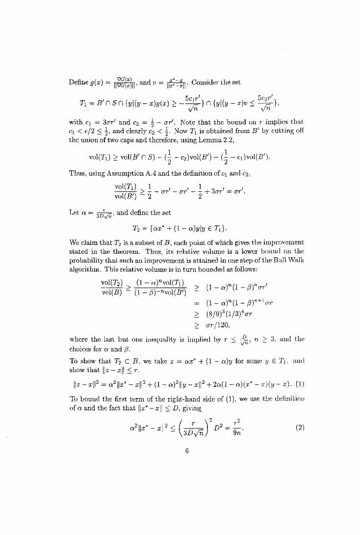
Define g(x) = lI~g~~~II' and v = II~:=~II' Consider the set

with Cl = 30-r' and C2 = ~ o-r', Note that the bound on r' implies that Cl < t/2 :s; ~, and clearly C2 < ~. Now Tl is obtained from B' by cutting off the union of two caps and therefore, using Lemma 2.2,

vol(Td 2:: vol(B' n S) (~ - c2)vol(B') - (~ cl)vol(B'). 2 2

Thus, using Assumption AA and the definition of Cl and C2,

Let a =

vol(Tt} 1 , vol(B') 2:: 2 - o-r

and define the set

I 1 I I 0-'[' - 2 + 30-r = o-T .

T2 = {ax* + (1 a)yly E Td·

We claim that T2 is a subset of B, each point of which gives the improvement stated in the theorem, Thus, its relative volume is a lower bound on the probability that such an improvement is attained in one step of the Ball Walk algorithm, This relative volume is in turn bounded as follows:

vol(T2) > (1 - a)nvol(Td vol(B) - (1- J3)- n vol(B')

> (1

= (1 at(1- (3)71+l0-'t

> (8/9)3(1/3)40- r

> o-r/120,

where the last but one inequality is implied by r::; , 11, 2:: 3, and the choices for a and (3,

To show that T2 c B, we take z = ax* + (1 a)y for some y E T j • and show that liz - xii :s; r.

liz xl1 2 = a211x* - xl12 + (1 - a)211y - xl12 + 2a(1 - a)(x* - :I;)(Y - :I:). (1)

To bound the first term of the right-hand side of (1), we use the definitiolJ of a and the fact that Ilx* xii::; D, giving

(2)

6

Since y E B' implies that Ily - xii :S r' = (1 - fJ)r and 0 :S a, fJ :S 1 implies that (1 a)2(1 - fJ)2 :S (1 (3), the second term of the right-hand side is bounded by

(3)

Finally, the definitions of a, v, C2 and Tl imply

10 r2 5r2 2a(1 - a)(x* - x)(y x):s 3(1 - fJ)cz;::S 3n' (4)

(2), (3), (4) inserted in (1) yields

liz - xl12 :S (~+ 1 - 2 + ~) 1'2 :S r2. 9n n 3n

Next we show that z gives the desired improvement over x. By concavity of G

G(z) - G(x} 2:: a(G(x*) G(x)) + (1 - a)(G(y) - G(x)). (5)

The second order Taylor expansion of G in y around x yields

G(y) - G(x} = "VG(x)(y - x) + ~G"(w; x')lIy - xll 2

> _ 5c1r'II"VG(x)11 _ ~v1"2 fo 2

5cl1' 1 2 > - fo IlvG(x)1I - '2vr

15<1r2 1 2 > - fo II"VG(x)ll- '2v1' , (6)

where x' E [x, y], w = (y - x)/Ily - xii, and we used Assumption A.3 for the first inequality. Using the definition of a, (5) and (6) yield

G(z) G(x) 2:: 3;fo(G(x*) - G(x)) - (~ II"VG(x) II + ~v) 1'2.

Since we assumed G(x*) - G(x) 2:: €TD, using IlvG(x)11 :S T (Assumption A.2), leads to

G(z) - G(x) > l' _ (15CJT/fo + V/2) 1'2. G(x*) - G(x) - 3Dfo €TD €TD

Since l' :S 90lTTr-3v\l1i' a simple calculation now gives

G(z} G(x} > _1'_ G(x*) - G(x) - 6Dfo

o

7

The justification of the Ball Walk algorithm follows as a corollary.

Theorem 2.2 The number of samplings from a ball that Ball Walk requires to reach, with probability at least 1 -1], a point x with G(x*) - G(:r;) S; ET D is bounded from above by

720foD In(l/E) In (6foD In(l/E)) . ~r2 1]r

PROOF. The probability of finding an improving point given in Theo­rem 2.1 implies that, if the inner loop of the Ball Walk algorithm runs

120 In (6.JnD1n(l/€)) of times. then the probability of incorrect termination OT 1JT '

. 9T 1S at most 6.JnDln(1/€)'

The one step improvement in Theorem 2.1 implies

G(x*) - G(z) < 1 _ r

G(x*) - G(x) -

Moreover, by concavity of G and Assumption A.2, G(x*) for any feasible point y, hence also for the starting point. improvement steps we obtain a point xk with

Therefore, log(l/E) < 6foDlog(1/E)

log (6foD/(6foD - r)) - r

G(y) ::; TD Thus, after k

improvement steps are sufficient to obtain the desired precision €T D. Mul­tiplying the error probability of incorrect termination by the number of improvement steps yields the overall incorrect termination is bounded by 1]. 0

Note that the bound of Theorem 2.2 is indeed polynomial in the parameter::; of the problem, since r is a rational function of the problem parameters.

3 Two-stage stochastic programming

In this section we describe briefly stochastic linear programming problems. Problems of this type have been studied since they were proposed in t,lw

8

mid 1950's [2], [4], [17]. They model optimisation under uncertainty. Such models are useful in many practical situations. Obtaining exact information about all parameters in a practical optimisation problem is often impossi­ble.

As an example, think of allocating funds to a variety of possible investments 1)0 as to maximise profit under a budget restriction. Usually at the moment the investment decision is to be made there is no certainty at all about the future yields of the various investments. Neither might there be exact information about the amounts needed to invest in a certain given project. At best one might hope to have some idea of what these parameter values could be, and to express this in the form of probability distributions. In this way we arrive at stochastic programming problems.

Suppose that we have a linear programming problem in which some param­eters are random. The random variables we indicate by putting a tilde over them.

max px

subject to Ax:S b - -Tx:S ~

with b E l!{m, e E l!{d, and A an m x n matrix, T an d x n matrix, and pEl!{n.

We a,.-;sume that probability distributions are given for the random matrix T and the random vector e. The above model is clearly ill-defined since a solution x that is optimal for one realisation of T and { may even be infeasible for another.

Two main directions have been taken in the literature to arrive at sensible models. In the conceptually easiest, violation of the uncertain constraints is allowed to occur with a probability that does not exceed a prespecified level, giving the so-called probabilistic constraints problem. The best comprehen­sive survey of this field is [16]. The paper of Kannan and Nolte [13] takes a similar approach to the probabilistic constraints problem that we take here for the model described next.

The other approach is the one we consider in this paper and is called the t'IVO-8t(J,gl? stochastic programming problem or the stochastic recourse problem.

9

Conceptually one should think of the decision process taking place in two stages. In the first, values for the first stage variables x are chosen. In the second, upon a realisation of the random parameters, a recourse action is to be taken in case of infeasibilities. Costs are attached to the various possible recourse actions leading to the second stage (or recourse) problem, to choose the optimal action given the infeasibilities. The expected cost of the optimal recourse action is then added to the objective function. For a comprehensive review of the extensive literature we refer to [3], [8], [16].

A generic mathematical programming formulation for this problem is

max px + E[max{qy I Wy :s; Tx -(, y E ~nl}] subject to Ax:S; b.

(7)

with q E JR"'1 and W an d x nl matrix. In the literature W is sometimes allowed to be a random matrix. However, this may cause the feasible region to be non-convex in terms of x (see [18]). We concentrate 011 the so-called fixed recourse model in which W is fixed. Moreover, we assume that W is such that for any x and any realisation of T and l there exists a feasible solution y in the second stage problem. This property of W is called the complete recourse property, and the model is accordingly called t.he complete recourse model (see e.g. [3]).

It is well known that the objective function of (7) is concave (see [19, 18]). Therefore, the two-stage stochastic programming problem boils down to maximising a concave function over a convex (polyhedral) set. Thus, we can use our Ball Walk algorithm to solve this problem if we know that the objective function and the convex feasible set satisfy our smoothness conditions. It will be clear that this is not true for the feasible set, which is a polyhedron. We will come to this point later, in Section 6. However, another serious obstruction against using Ball Walk is that this algorithm requires an oracle that gives function values on request. As will be clear from the next section, it is exactly the evaluation of the objective function which makes the two-stage stochastic programming problem so excessively hard to solve. Therefore, the assumption that a function evaluation oracle exists for these problems significantly hides their computational difficulty.

Therefore, before adapting the Ball Walk algorithm to solve two-stage ::;toclms­tic programming problems in Section 6, we first devise a suita.ble fUllction evaluation oracle in Section 5.

10

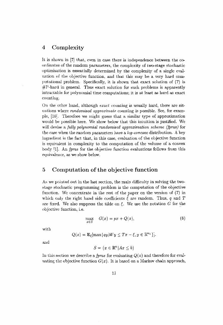
4 Complexity

It is shown in [7J that, even in case there is independence between the co­ordinates of the random parameters, the complexity of two-stage stochastic optimisation is essentially determined by the complexity of a single eval­uation of the objective function, and that this may be a very hard com­putational problem. Specifically, it is shown that exact solution of (7) is #P-hard in generaL Thus exact solution for such problems is apparently intractable for polynomial time computations; it is at least as hard as exact counting.

On the other hand, although exact counting is usually hard, there are sit­uations where randomised approximate counting is possible. See, for exam­ple, [10J. Therefore we might guess that a similar type of approximation would be possible here. We show below that this intuition is justified. We will devise a fully polynomial randomised approximation scheme (fpras) for the case when the random parameters have a log-concave distribution. A key ingredient is the fact that, in this case, evaluation of the objective function is equivalent in complexity to the computation of the volume of a convex body [1]. An fpras for the objective function evaluations follows from this equivalence, as we show below.

5 Computation of the objective function

As we pointed out in the last section, the main difficulty in solving the two­stage stochastic programming problem is the computation of the objective function. We concentrate in the rest of the paper on the version of (7) in which only the right hand side coefficients €are random. Thus, q and T a.re fixed. We also suppress the tilde on ~. We use the notation G for the objective function, i.e.

max G(x} = px + Q(x), xES

(8)

with Q(x) = Edmax{qyIWy:S Tx - Cy E ]Rnl }].

and s = {x E ]RnlAx :S b}

In this section we describe afpras for evaluating Q(x) and therefore for eval­uating the objective function G(x). It is based on a Markov chain approach,

11

where we sample approximately according to the known density function of ~, compute the value of the linear program and take the average over the values obtained from the sample.

The only source ofrandomness is~, which we assume is described by a given density function f : ]Rd -+ R Thus,

Q(x) = J v(Tx - Of(Od~

with v(Tx -~) = max{qYIWy ::; Tx -~, Y E ]Rnl}.

We require some mild conditions on f. We cannot expect to approximate Q efficiently for arbitrary f, since it is known that there exist counting functions which are NP-hard to approximate [10]. Therefore we assume the following conditions, borrowed from volume computation [1].

Assumptions B:

1. f is log-concave, i.e. log f is concave on its support supp f;

2. f has a negligible measure outside B(O, R), i.e. there exists R ~ 4d

such that ~I~II~R f(Od~ ::; <p, for some <Pi

3. log f is Lipschitz-continuous, i.e. there exists () > ° such that I log f (e)­logf(e)1 ::; Bile - ell for all e,e E suppf;

4. We are given a eo E B(O, R) with f(eo) ~ R-"Id for some absolute constant T. This implies that we know a good starting point for the Markov chain, a so called "warm start,,;4

5. v is uniformly bounded, i.e. there exists L such that for all ~ E supp f and xES, Iv(Tx - ~) I ::; L;

6. The rows of T are scaled to have unit norm. Thus IITII ::;Jd.

7. There exist Xo E ]RTL, Rin, Rout E ll4 such that B(xo, Rill) ~ S c B(xo, Rout).

4If necessary, such a point can be found with a preliminary convex optimisation.

12

These conditions do not severely restrict the instances, since (with minor technical changes) all the most important distributions, for example those from the exponential family, meet the requirements.

Condition B.5 is a little more restrictive than the usual assumption in two­stage stochastic programming that the function v is bounded. Boundedness only is already assured if E[e] is finite (see e.g. [18]). Condition B.6 is clearly not restrictive, and B.7 is discussed in the next section. We don't use either of B.6 or B. 7 until the following section, but give them here to have a complete overview of all our conditions.

To sample according to f, we define a Metropolis random walk that has f restricted to B(O, R) as its steady state density function. Note that, by Assumption B.2, the restricted density j satisfies f s: j s: f /(1- ~). If ~ is assumed negligible, we can suppose that this simply contributes a negligible amount to the approximation error for Q(x). Thus we will not need to draw a distinction between f and j in what follows and we will use the notation f, though it should read j. To sample from f we define a random walk that has f as its steady state density. One step of the random walk is defined as follows. Suppose the walk is at x E B(O, R). We choose uniformly at random a point y in a ball with center x and radius 6, to be specified later. If y is not in B(O, R), we stay at x. Otherwise, if f(y) :2: f(x), we move to y, else we move to y with probability f (y) / f (x). Formally, the transition kernel p( x, y) (x i= y) for moving from x to y in one step of the random walk is given by

p(x,y) {

VOl(B~O, 0)) min {I, ~~~~} if y E B(O, R), 0 < Ilx - yll s: 0,

o otherwise.

Not.e that p(x, x) is an atom 1 fy:;i:x p(x, y) dy. It is easy to see, by time re­versibility, that the steady state distribution of this random walk has density proportional to f (x).

In the following we will use techniques and results from volume estimation [6, 12] to prove that this chain mixes rapidly, i.e. converges fast to the steady state. We first introduce some notation and state the relevant results from the literature.

Theorem 5.1 Dyer and Frieze [5} Let S C ~d be a convex body with diameter D and f be a log-concave function deEned on S with 'IT the induced measure. Let 8 1,82 C S, t s:

13

dist (8I, 82) = minx ESbYES2 Ilx - yll· If 80 = S \ (81 U 82)), tilen

min{ 1r(81), 1r(8z)} S ~ 1r(80).

2/d is called tile isoperimetric constant 180(S) of S. o

Given a random walk with stationary distribution 1r defined on a set S, its conductance is defined as

<P = inf {scslo<w(S):::;1/2}

Is Pu(8)d1r(u) 1r(8)

where Ptt (8) is the probability of moving in one step from point u in 8 C S to a point in 8, the complement of 8 in S.

The local conductance of a Markov chain at a point x is defined as the probability of moving to any point y #- x in one step.

Theorem 5.2 Kannan [11] Consider a Metropolis random walk using balls of radius c5 ill a convex set S C ]Rd wilich has local conductance at least X at every point. Tilell tile conductance q> of the walk is at least

o

Theorem 5.3 Lovasz and Simonovits [14] Let io be the initial density of a Markov chain on lRd with statiollary density i. Define

MUo, f)= sup {SClll:dlo<fs f-5:1/2}

I Isi - Isiol

Jisi Let ik be the density of the Markov chain after k steps. Then

o

14

Procedure Estimate begin

Q t- 0;

K t- i8L21;PIP) l ; for 1; t- 1, ... , K do;

run the Metropolis walk for K' steps, starting from eo; compute v(Tx - 0 for the resulting sample e; Q t- Q + v(Tx - e);

endfor;

Q t- 9.. K'

Figure 2: The approximation algorithm for Q(x)

Theorem 5.4 Using the Metropolis random walk, we can sample in B(O, R) C lRd according to a density f' with sUPSClRd 1 Is f - Is /,1 < E in K' steps, where

PROOF. Theorem 5.1 gives an isoperimetric constant of -h for a random walk on B(O, R). The Lipschitz continuity (Assumption B.3) implies that the acceptance function varies only by a constant factor over B(x, (5). Thus, choosing 6 Ja implies a constant local conductance, since vol(B(x, 6) n B(O, R)) ::: O.4B(x, (5), if x E B(O, R). To see this note that the intersection contains a cap of B(x, 6) of distance at most 62 /(2R), by elementary geom­etry. Lemma 2.2 with c = 1/(2R) now implies the volume of the cap is at least 1/2 1/(3R) > 0.4, by Assumption B.2.

Applying these results, Theorem 5.2 implies a lower bound on the conduc­tance .;p of the walk of 2oJRd' Theorem 5.3 then yields

We choose the uniform distribution on B(eo,6) as the initial density fo, where eo is the point guaranteed by Assumption BA. Assumption B.3 again implies that the acceptance function varies over B(eo, (5) only by a factor eo. These, together with Assumption B.2, imply MUo, 1) ORC-y+l)d, after some calculation. 0

In Figure 2 we define the procedure Estimate based on the Markov chain described above to compute an approximation of the value of Q( x).

15

Theorem 5.5 With probabilityl-p, Procedure Estimate computes QJdx) E

[Q(x) - €,Q(x) + €] in KK' = a (,R2€13L21og Of logRIog~) steps.

PROOF. Let QK(X) = k 2:~1 v(Tx - ~i)' with 6,'" ,eK independent samples generated by the Metropolis random walk. Thus, E[QK(X)] =

f v(Tx ~)fK'(e)de, where fK' is the density produced by the Metropolis random walk when run with error parameter f.' = €/4L. Since v is bounded by L by Assumption B.5, Hoeffding's inequality implies

Pr{IQK(x) - E[QK(X)]I > !f.} :$ 2exp ( - ~:5) , since K 2:: 8L2 ln(21 p)c2 . Theorem 5.4 yields

IE[QK(X)] - Q(x)1 II v(Tx OfK'(Od~ - I v(Tx Of (Ode I < L I If(e) - fK'(~)lde

- 2L r (jK,(e) - f(O)de } f:5:fK'

< 2Lf.' = ~f.,

Combining these, we see that Pr{IQK(x) - Q(x)1 > f.} :$ p. o

Using the approximation algorithm for the objective function G and apply­ing the ellipsoid algorithm in [9] to our problem, under our assumptions we would have a fpras for the stochastic recourse problem. The following theorem follows easily from taking p (IN in Theorem 5.5, where N is the required number of steps of the ellipsoid algorithm.

Theorem 5.6 Under Assumptions B.I-B.5, with probability at least 1- (, the ellipsoid algorithm, using procedure Estimate to approximately evaluate G, will solve the two-stage stochastic programming problem (8) to within additive error €, in a number of arithmetic operations bounded polynomially in the input parameters, 1/f. and log 1/(. 0

The ellipsoid algorithm is complicated to apply and can be very ~low. There­fore we combine the method for approximate function evaluations with the method of Section 2 to obtain a simple randomized local improvement al­gorithm. Our earlier results will then imply that, with high probability, a solution is obtained that is close to the optimaL

16

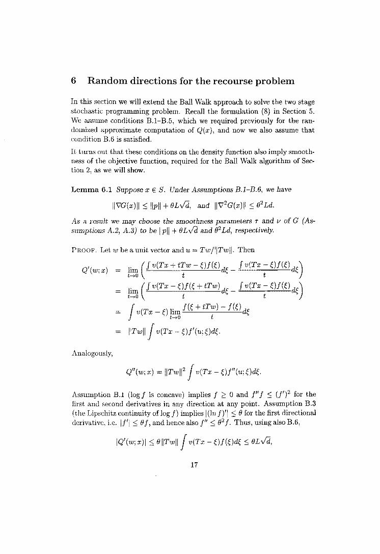
6 Random directions for the recourse problem

In this section we will extend the Ball Walk approach to solve the two stage stochastic programming problem. Recall the formulation (8) in Section 5. We assume conditions 8.1-8.5, which we required previously for the ran* domized approximate computation of Q(x), and now we also assume that condition 8.6 is satisfied.

It turns out that these conditions on the density function also imply smooth­ness of the objective function, required for the Ball Walk algorithm of Sec­tion 2, as we will show.

Lemma 6.1 Suppose xES. Under Assumptions B.l-B.6, we have

II\7G(x)II ~ Ilpll + BLVd, and 11\72G(x)11 ~ 02 Ld.

As a result we may choose the smoothness parameters 'T and lJ of G (As­sumptions A.2, A.3) to be Ilpll + BLVd and B2 Ld, respectively.

PROOF. Let w be a unit vector and u = Tw/IITwll. Then

.. J v(Tx - Of(O de) Q'(w;x) = lim "---'-------'-'-'---'--'-at - ., t-tO t t

= lim (J v(Tx e)f(e + tTw) d~ _ J v(Tx - ~)f(~) d~) t-tO t t

= !V(TX e)limf(~+tTw)-f(Ode t-tO t

= IITwll ! v(Tx - e)i'(u;e)de.

Analogously,

Q"(W; x) = IITwl12 / v(Tx - Oi"(u; Ode.

Assumption B.1 (log f is concave) implies f 2': 0 and 1" f ~ (f')2 for the first and second derivatives in any direction at any point. Assumption B.3 (the Lipschitz continuity of log f) implies I (In f)'1 ~ 0 for the first directional derivative, i.e. If'l ~ Of, and hence also 1" ~ 02f. Thus, using also 8.6,

IQ'(w;x)1 ~ OllTwl1 / v(Tx - e)f(~)de ~ OLVd,

17

and

QfI(W;X) ~ e2 11Twl12 J v(Tw Of(~)d~ ~ (PLd.

Therefore we have, for all x, w,

IG'(w;x)1 ~ Ilpll +811TIIL and GI/(w;x) = Q"(w;x) ~ e2 11T11 2L.

The lemma follows. o

Thus, Assumptions A.2 and A.3 in Section 2 are satisfied. We know that Gis concave, satisfying also Assumption A.I. Therefore, we need to be concerned now with smoothing the underlying feasible set 8 = {x E JRn lAx:::; b}. Sino-; 8 is a polyhedron, it is not smooth. Therefore we use the "roundedness" Assumption B.7 on 8. This allows us to consider a slightly larger (non­polyhedral) set, which is indeed smooth, and apply the Ball Walk to this larger set.

Let K, = Rout! Rin, where Rin and Rout are the constants from Assumption B.7. We call K, the rounding number of the polytope. Note that K, resembles a "condition number": it is small if the polytope is "well-rounded" and large if it is not. Thus we will assume K, is not too large. In fact any polytope can be "rounded" to have K, = O( In), but here this may be undesirable since it can adversely affect the parameters of G. From now on we astlume that 8 satisfies the above assumption.

To facilitate the exposition, let A(i} denote the ith row of A, and tlUPP0tl€ A is normalised so that IIA(i) II = 1 (i = 1, ... , m). Then, for x E JRn , let

bi if A(i)x > bi, otherwise,

be the distance from x to the halfspace A(i)y ~ bi. Consider the function F(x) = L:~l ((A(i)x - bi)+)2, and, for a given I-" > 0, define the set 8 11. = {x E JRn IF (x) :::; I-"}. Note that 8 ~ 8 J1. and 8 J.t is convex. The following lemmas establish the required smoothness condition for 8 J.t'

Lemma 6.2 For all x,z E JRn , Ilzll = 1, 0 ~ F"(z;x) ~ 2m.

PROOF. We have

"VF(x) = 2 I.: (A(i)x - bi)A(i) , iEI(x)

18

(9)

where I(x) = {i : A(i)x > bd. Hence

V 2F(x) = 2 L A(i) A(i)T,

iE/ex)

(10)

and so F"(z;x) = 2 LiEI(x)(A(i)z)2. Clearly F"(z;x} 2: 0, and the upper bound follows from the Cauchy-Schwarz inequality and II(x)1 ~ m. 0

In particular, it follows that F is a convex function.

Lemma 6.3 Let 8 have rounding number K, and ° < /-L ~ 1. Then, for all :c E 8/1.,

PROOF. Assume without loss that Xo = o and Rin = 1, so Rout = K,. Also bi 2: 1 (i = 1, ... ,m), by considering the points A(i) E 8B(O, 1). Fix x E 8ILl

let

and let £ be the minimizing i. Let x = Ax/llxll, so A = Ilxll. Clearly A ~ K" Hiuce otherwise A(i)x ~ bi (i = 1, ... ,m), but x ~ B(O, K,). Now

-Jii. 2: -Jii./bl 2: (A(l)x - be)/bl = Ilxll/A - 1 = Ilxll/llxll - 1.

Thus Ilxll ~ (1 + VIi) Ilxll ~ 2K,. Thus, from (9),

xVF(:c) = 2 L (A(i)x - bi)A(i)x 2: 2 L (A(i)x - bi) 2: 2VF (x),

iEI(x) iEl(x)

since A(i);c > bi 2: 1 for i E I(x) and F(x) LiE/(X)(A(i)x-bi )2. Therefore, using Caudw-Schwarz,

IIVF(x)11 2: 2VF(x)/llxll 2: VF(x)/K"

and the result follows. o

Lemma 6.4 Let 0 < /-L ~ 1, and a = (4mK,/3)Vn//-L. Then, for all x E 8 ,1.)

vol(B(x, r) n 8p,)/vol(B(x, r)) 2: ~ - aT.

19

PROOF. Assume without loss that x is on the boundary of Sfl" Using Taylor's theorem and Lemma 6.2, for any displacement z,

F(x + z) ::; F(x) + z'VF(x) + 2mz2 = J.L + z'VF(x) + 2mz2,

and the subgradient inequaility gives

F(x + z) ~ F(x) + z'VF(x) = J.L + z'VF(x).

Thus, if F(x + z) = J.L, -2mz2 ::; zYF(x) ::; O. Let H denote the half-space z'VF(x) ::; 0, and oH its boundary. Then, using Lemma 6.3,

. -z'VF(x) 2mz2 2mr.z2 2mr.z2 dlst (z,oH) = II'VF(x)II ::; II'VF(x) II ::; JF(x) = Vii

Letting B denote B(x, r), we see that BnSfJ. contains a cap of B at distance at most 2mr.r2/ Vii from x. Thus, by Lemma 2.2,

vol(B n SfJ.) 1 4mr.y'n -~-...!::.:->-- r.

vol(B) - 2 3Vii

o

Using the last two lemmas we can now apply the Ball Walk to optimize Gover Sp,- But, we are of course interested in optimizing G over the set S C Sp,- Thus, we will use Procedure Near (see Figure 6), which finds a point arbitrarily close to S after we have optimized over the larger set Sp,- The idea is to go repeatedly along the gradient of F, which is easy to compute, until we are exponentially close to S. We will show that thiH procedure yields a point that is not much worse than the point resulting from the Ball Walk Algorithm, for an appropriate choice of J.L.

Theorem 6.1 Let x E SfJ.' For any (3 < J.L, Procedure Near finds y E S{'! with Ilx - yll ::; 2Jp,/{31n(p,/{3). The running time is O(r.2m 2n In(fl'/{3))·

PROOF. The claim on the running time is easy to verify. Without loss, we will prove the lemma for a point x on the boundary of SJ.L' i.e. F(x) = fl ..

We start the procedure at x with F(x) = J.L and

A JF(x) 'VF(x) x=x- .

2Km II'VF(x)II

20

Procedure Near(x, p) begin

lend;

For i = 1 to r 4f1:2m In(/-L/ p)l do; Calculate F(x), vF(x)

x = x yF(x) 'ilF x 21'r-m I'ilF(x I

x =x; endfor; return x;

Figure 3: The Procedure Near

Using Lemma 6.2, the Taylor expansion yields

F(x) :" F(x) _ ~11V'F(x)11 + m ( ~) 2

Now, using Lemma 6.3, this implies

F(x) ~ F(x)

We repeat t.his process k 4f1:2m log(/-L/ p) times to get a point y with

Furthermore, letting y be the final point returned by Near,

Hence, using t.he subgradient inequality,

G(y) ~ G(x) - Tlly - xii ~ G(x) 2Tf1:.Jii In(/-L/p).

21

Thus, since J1 ::; 1, we will have G(y) ?: G(X)-E provided

J1 ::; (2T1d~(1/ /1)) 2 (11)

Note that this is polynomial in the relevant parameters, in particular the number of bits of accuracy required. 0

Collecting the last results and inserting the right parameters in the general time bounds of the Ball Walk we get our final result.

Theorem 6.2 Under the Assumptions B.l-B. 7; with probability at least (1 - (), an application of the Ball Walk combined with the procedures timate and Near wjJ1 find ywitll

G(y) ?: G(x*) - E

and Ay ::; b + J73,

in time polynomial in the parameters of the problem, liE, log(l/t1) and log(1/()·

PROOF. By using a small enough error probability at each step, the proba­bility of making an error can be made at most ( over any polynomial number

2 of steps (cf. the discussion before Theorem 5.6). Choose J1 = Lemmas 6.1, 6.4 and Theorems 5.5, 6.1 then imply the theorem. 0

7 Postlude

We have described a simple randomized approximation scheme for convex optimisation problems, with two-stage stochastic programming problems as the main application. Whether the method that we propose here is a prac­ticallyefficient method for solving two-stage stochastic programming prob­lems remains to be seen, but in any case it may provide a starting point for a more practical method. For example, it is likely that function evaluations do not have to be so precise if we are still far away from the optimum. Indeed. stochastic programmers have proposed methods that work with lllore awl more accurate function evaluations as their methods proceed. It remain . ., a challenge to incorporate these and other ideas that have been developed ill stochastic programming research into our algorithmic framework.

22

References

[1] Applegate, D., Kannan, R. Sampling and integration of near log­concave functions. Proceedings of the 23th A CM Symposium on the Theory of Computing, 1990, pp. 156-163,

[2] Beale, E.M. On minimizing a convex function subject to linear inequal­ities. Journal of the Royal Statistical Society 17, 1955, pp. 173-184.

[3] Birge J., Louveaux F. Introduction to stochastic programming, Springer­Verlag, New York, 1997.

[4] Dantzig, G. Linear Programming under uncertainty. Management Sci­ence 1, 1955, pp. 197-206.

[5] Dyer, M. and Frieze, A. Computing the volume of convex bodies: a case where randomness provably helps. Probabilistic Combinatorics and its Applications, Proceedings of AMS Symposia in Applied Mathematics VoL 44, 1991, pp. 123-169.

[6] Dyer, M., Frieze, A., Kannan, R. A random polynomial time algorithm for approximating the volume of convex bodies. Journal of the ACM 38, 1991, pp. 1-17.

[7] Dyer, M., Stougie, L. A note on the complexity of some stochastic optimization problems, preprint.

[8] Ermoliev Y, Wets R. (eds.) Numerical techniques for stochastic opti­mization, Springer-Verlag, Berlin, 1988.

[9] Grotschel, M., Lovasz, L., Schrijver, A. Geometric algor'ithms and com­lrtnatorial optimization. Springer Verlag, New York, 1988.

[10] Jerrum, M., Sinclair, A. The Markov chain Monte Carlo method: an approach to approximate counting and integration. In Approximation (J,lgorithms for NP-hard problems, D. S. Hochbaum (ed.), PWS Publish­ing, Boston, 1996, pp. 482-520.

[11] Karman, R. Markov chains and polynomial time algorithms. Proceedings of the 35th Symposium on Foundations of Computer Science, 1994, pp. 656-671.

23

[12] Kannan, R., Lovasz, L., Simonovits, M. Random walks and an O*(n5)

volume algorithm for convex bodies. Random Structures and Algorithms 11, 1997, pp. 1-50.

[13] Kannan, R., Nolte, A. Local search in smooth convex sets. Proceed'ings of the 39th Symposium Or! Foundations of Computer Science, 1998, pp. 218-226.

[14] Lovasz, L., Simonovits, M. Random walks in a convex body and an im­proved volume algorithm. Random Structures and Algorithms 4, 1993, pp. 359-412.

[15] Nemirovski, A., Nesterov. Y. Interior point polynomial methods in con­vex programming, SIAM Press, 1994.

[16] Prekopa, A., Stochastic programming, Mathematics and its applications Vol. 324, Kluwer, Dordrecht, 1995.

[17] Tintner, G. Stochastic linear programming with applications to agricul­tural economics. In Antosiewicz, H.A. (ed.) Proceedings of the Second Symposium on Linear Programming, Washington, 1955, pp. 197-207.

[18] Wets, R. Stochastic programming: solution techniques and approxi­mation. In Bachem, A., Groetschel M., Korte, B. (eds.) Mathematical programming: the state of the art (Bonn, 1982), Springer, Berlin, 1983, pp. 566-603.

[19] Wets, R. Stochastic programming. In Optimization, Handbooks of Op­erations Research and Management Science Vol. 1, North-Holland, Am­sterdam, 1989, pp. 573-629.

24