ILSB Report 206 hjb/ILSB/220131

ILSB Report / ILSB-Arbeitsbericht 206(supersedes CDL–FMD Report 3–1998)

A SHORT INTRODUCTION

TO BASIC ASPECTS

OF CONTINUUM MICROMECHANICS

Helmut J. Bohm

Institute of Lightweight Design and Structural Biomechanics (ILSB)Vienna University of Technology

updated: January 31, 2022c©Helmut J. Bohm, 1998, 2022

Contents

Notes on this Document iv

1 Introduction 11.1 Inhomogeneous Materials . . . . . . . . . . . . . . . . . . . . . . . . . . . . 11.2 Homogenization and Localization . . . . . . . . . . . . . . . . . . . . . . . 41.3 Volume Elements . . . . . . . . . . . . . . . . . . . . . . . . . . . . . . . . 61.4 Overall Behavior, Material Symmetries . . . . . . . . . . . . . . . . . . . . 71.5 Major Modeling Strategies in Continuum Micromechanics of Materials . . 91.6 Model Verification and Validation . . . . . . . . . . . . . . . . . . . . . . . 14

2 Mean-Field Methods 162.1 General Relations between Mean Fields in Thermoelastic Two-Phase Materials 162.2 Eshelby Tensor and Dilute Matrix–Inclusion Composites . . . . . . . . . . 202.3 Some Mean-Field Methods for Thermoelastic Composites with Aligned Rein-

forcements . . . . . . . . . . . . . . . . . . . . . . . . . . . . . . . . . . . . 232.3.1 Effective Field Approaches . . . . . . . . . . . . . . . . . . . . . . . 242.3.2 Effective Medium Approaches . . . . . . . . . . . . . . . . . . . . . 302.3.3 Hashin–Shtrikman Estimates . . . . . . . . . . . . . . . . . . . . . 32

2.4 Other Analytical Estimates for Elastic Composites with Aligned Reinforce-ments . . . . . . . . . . . . . . . . . . . . . . . . . . . . . . . . . . . . . . 33

2.5 Mean-Field Methods for Nonlinear and Inelastic Composites . . . . . . . . 352.5.1 Viscoelastic Composites . . . . . . . . . . . . . . . . . . . . . . . . 352.5.2 (Thermo-)Elastoplastic Composites . . . . . . . . . . . . . . . . . . 36

2.6 Mean-Field Methods for Composites with Nonaligned Reinforcements . . . 412.7 Mean-Field Methods for Non-Ellipsoidal Reinforcements . . . . . . . . . . 452.8 Mean-Field Methods for Coated Reinforcements . . . . . . . . . . . . . . . 482.9 Mean-Field Methods for Conduction and Diffusion Problems . . . . . . . . 49

3 Bounding Methods 553.1 Classical Bounds . . . . . . . . . . . . . . . . . . . . . . . . . . . . . . . . 553.2 Improved Bounds . . . . . . . . . . . . . . . . . . . . . . . . . . . . . . . . 593.3 Bounds on Nonlinear Mechanical Behavior . . . . . . . . . . . . . . . . . . 603.4 Bounds on Diffusion Properties . . . . . . . . . . . . . . . . . . . . . . . . 613.5 Comparisons of Mean-Field and Bounding Predictions for Effective Thermo-

elastic Moduli . . . . . . . . . . . . . . . . . . . . . . . . . . . . . . . . . . 613.6 Comparisons of Mean-Field and Bounding Predictions for Effective Con-

ductivities . . . . . . . . . . . . . . . . . . . . . . . . . . . . . . . . . . . . 68

ii

4 General Remarks on Modeling Approaches Based on Discrete Micro-structures 704.1 Microgeometries and Volume Elements . . . . . . . . . . . . . . . . . . . . 704.2 Boundary Conditions . . . . . . . . . . . . . . . . . . . . . . . . . . . . . . 774.3 Numerical Engineering Methods . . . . . . . . . . . . . . . . . . . . . . . . 804.4 Evaluation of Results . . . . . . . . . . . . . . . . . . . . . . . . . . . . . . 86

5 Periodic Microfield Approaches 905.1 Basic Concepts of Periodic Homogenization . . . . . . . . . . . . . . . . . 905.2 Boundary Conditions . . . . . . . . . . . . . . . . . . . . . . . . . . . . . . 925.3 Application of Loads and Evaluation of Fields . . . . . . . . . . . . . . . . 1005.4 Periodic Models for Composites Reinforced by Continuous Fibers . . . . . 1045.5 Periodic Models for Composites Reinforced by Short Fibers . . . . . . . . . 1105.6 Periodic Models for Particle Reinforced Composites . . . . . . . . . . . . . 1165.7 Periodic Models for Porous and Cellular Materials . . . . . . . . . . . . . . 1235.8 Periodic Models for Some Other Inhomogeneous Materials . . . . . . . . . 1275.9 Periodic Models Models for Diffusion-Type Problems . . . . . . . . . . . . 130

6 Windowing Approaches 132

7 Embedding Approaches and Related Models 137

8 Hierarchical and Multi-Scale Models 143

9 Closing Remarks 147

Bibliography 149

iii

Notes on this Document

The present document is an expanded and modified version of the CDL–FMD report3–1998, “A Short Introduction to Basic Aspects of Continuum Micromechanics”, which,in turn, is based on lecture notes prepared for the European Advanced Summer SchoolsFrontiers of Computational Micromechanics in Industrial and Engineering Materials heldin Galway, Ireland, in July 1998 and in August 2000. Related lecture notes were used forgraduate courses in a Summer School held at Ameland, the Netherlands, in October 2000and during the COMMAS Summer School held in September 2002 in Stuttgart, Germany.All of the above documents, in turn, are closely related to the micromechanics section ofthe lecture notes for the course “Composite Engineering” (317.003) offered regularly atVienna University of Technology.

The course notes “A Short Introduction to Continuum Micromechanics” (Bohm, 2004)for the CISM Course on Mechanics of Microstructured Materials held in July 2003 inUdine, Italy, may be regarded as a compact version of the present report that employsa somewhat different notation. The course notes “Analytical and Numerical Methods forModeling the Thermomechanical and Thermophysical Behavior of Microstructured Mate-rials” (Bohm et al., 2009) are also related to the present report, but emphasize differentaspects of continuum micromechanics, among them the thermal conduction behavior ofinhomogeneous materials and the modeling of cellular materials.

The present document is being updated periodically to reflect current developments incontinuum micromechanics as seen by the author; the most recent version can be accessedvia https://www.ilsb.tuwien.ac.at/links/downloads/ilsbrep206.pdf. The August12, 2015 version of this report can be accessed via the DOI: 10.13140/RG.2.1.3025.7127.

A Voigt/Nye notation is used for the mechanical variables in chapters 1 to 3. Tensorsof order 4, such as elasticity, compliance, concentration and Eshelby tensors, are written as6×6 quasi-matrices, and stress- as well as strain-like tensors of order 2 as 6-(quasi-)vectors.These 6-vectors are connected to index notation by the relations

σ =

σ1σ2σ3σ4σ5σ6

⇔

σ11σ22σ33σ12σ13σ23

ε =

ε1ε2ε3ε4ε5ε6

⇔

ε11ε22ε33γ12γ13γ23

,

iv

where γij = 2εij are the shear angles1 (“engineering shear strains”). Tensors of order 4 aredenoted by bold upper case letters, stress- and strain-like tensors of order 2 by bold lowercase Greek letters, and 3-vectors by bold lower case letters. Conductivity-like tensors oforder 2 are treated as 3×3 matrices and denoted by calligraphic upper case letters. Allother variables are taken to be scalars.

In using the present notation it is assumed that the 4th order tensors show orthotropicor higher symmetry and that the material axes are aligned with the coordinate systemwhere appropriate. Details of the ordering of the components of ε and σ will not impactformulae. It is worth noting that with a notation like the present one some coefficients ofEshelby tensors differ compared to index notation, compare Pedersen (1983).

The tensorial product between two tensors of order 2 as well as the dyadic productbetween two vectors are denoted by the symbol “⊗”, where [η ⊗ ζ]ijkl = ηijζkl, and[a ⊗ b]ij = aibj, respectively. The contraction between a tensor of order 2 and a 3-vectoris denoted by the symbol “∗”, where [ζ ∗n]i = ζijnj. Other products are defined implicitlyby the types of quasi-matrices and quasi-vectors involved. A superscript T denotes thetranspose of a tensor or vector.

Constituents (phases) are denoted by superscripts, with (p) standing for a general phase,(m) for a matrix, (i) for inhomogeneities of general shape, and (f) for fibers. Axial and trans-verse properties of transversely isotropic materials are marked by subscripts A and T ,respectively, and effective (or apparent) properties are denoted by a superscript asterisk ∗.

The present use of phase volume fractions as microstructural parameters is valid for themicrogeometries typically found in composite, porous and polycrystalline materials. Notethat for penny shaped cracks a crack density parameter (O’Connell and Budiansky, 1974)is the proper choice.

1This notation allows strain energy densities to be obtained as the scalar product U = 12σ

Tε. Further-more, the stress and strain “rotation tensors” R∠

σand R∠

εfollow the relationship R∠

ε= [(R∠

σ)−1]T .

v

Chapter 1

Introduction

In the present report some basic issues of and some of the modeling strategies used forstudying static and quasistatic problems in continuum micromechanics of materials arediscussed. The main emphasis is put on application related (or “engineering”) aspects,and neither a comprehensive theoretical treatment nor a review of the pertinent literatureare attempted. For more formal treatments of many of the concepts and methods discussedin the present work see, e.g., Mura (1987), Aboudi (1991), Nemat-Nasser and Hori (1993),Suquet (1997), Markov (2000), Bornert et al. (2001), Torquato (2002), Milton (2002), Quand Cherkaoui (2006), Buryachenko (2007), Kachanov and Sevostianov (2013), Kachanovand Sevostianov (2018) as well as Buryachenko (2022); Yvonnet (2019) is specialized tonumerical continuum micromechanics. Shorter overviews of continuum micromechanicswere given, e.g., by Hashin (1983), Zaoui (2002) and Kanoute et al. (2009). Discussions ofthe history of the development of the field can be found in Markov (2000) and Zaoui (2002).

Due to the author’s research interests, more room is given to the thermomechanicalbehavior of two-phase materials showing a matrix–inclusion topology (“solid dispersions”)and, especially, to metal matrix composites (MMCs) than to materials with other phasetopologies or phase geometries, or to multi-phase materials.

1.1 Inhomogeneous Materials

Many industrial and engineering materials as well as the majority of biological materialsare inhomogeneous, i.e., they consist of dissimilar constituents (“phases”) that are dis-tinguishable at some (small) length scale(s). Each constituent shows different materialproperties and/or material orientations and may itself be inhomogeneous at some smallerlength scale(s). Inhomogeneous materials (also referred to as microstructured, hetero-geneous or complex materials) play important roles in materials science and technology.Well-known examples of such materials are composites, concrete, polycrystalline materials,porous and cellular materials, functionally graded materials, wood, and bone.

The behavior of inhomogeneous materials is determined, on the one hand, by the rel-evant material properties of the constituents and, on the other hand, by their geometryand topology (the “phase arrangement”). Obviously, the availability of information on

1

these counts determines the accuracy of any model or theoretical description. The behav-ior of inhomogeneous materials can be studied at a number of length scales ranging fromsub-atomic scales, which are dominated by quantum effects, to scales for which contin-uum descriptions are best suited. The present report concentrates on continuum modelsfor heterogeneous materials, the pertinent research field being customarily referred to ascontinuum micromechanics of materials. The use of continuum models puts a lower limiton the length scales that can be covered in a relatively carefree way with the methods dis-cussed here, which typically may be taken as being of the order of 1 µm (Forest et al., 2002).

As will be discussed in section 1.2, an important aim of bridging length scales for in-homogeneous materials lies in deducing their overall (“effective” or “apparent”) behavior2

(e.g., macroscopic stiffness, thermal expansion and strength properties, heat conductionand related transport properties, electrical and magnetic properties, electromechanicalproperties, etc.) from the corresponding material behavior of the constituents (as well asthat of the interfaces between them) and from the geometrical arrangement of the phases.Such scale transitions from lower (finer) to higher (coarser) length scales aim at achiev-ing a marked reduction in the number of degrees of freedom describing the system. Thecontinuum methods discussed in this report are most suitable for (but not restricted to)handling scale transitions from length scales in the low micrometer range to macroscopicsamples, components or structures with sizes of millimeters to meters.

In what follows, the main focus will be put on describing the thermomechanical be-havior of inhomogeneous two-phase materials. Most of the discussed modeling approachescan, however, be extended to multi-phase materials in a straightforward way, and thereis a large body of literature applying analogous or related continuum methods to otherphysical properties of inhomogeneous materials, compare, e.g., Hashin (1983), Torquato(2002) as well as Milton (2002), and see sections 2.9 and 5.9 of the present report.

The most basic classification criterion for inhomogeneous materials is aimed at the mi-croscopic phase topology. In matrix–inclusion arrangements (“solid suspensions”, as foundin particulate and fibrous materials, such as “typical” composite materials, in porous ma-terials, and in closed-cell foams3) only the matrix shows a connected topology and theconstituents play clearly distinct roles. In interpenetrating (interwoven, co-continuous,skeletal) phase arrangements (as found, e.g., in open-cell foams, in certain composites, orin many functionally graded materials) and in typical polycrystals (“granular materials”),in contrast, the phases cannot be readily distinguished topologically.

Obviously, an important parameter in continuum micromechanics is the level of inho-mogeneity of the constituents’ behavior, which is often described by a phase contrast. Forexample, the elastic contrast of a two-phase composite is typically defined in terms of thethe Young’s moduli of matrix and inhomogeneities (or reinforcements), E(i) and E(m), as

2The designation “effective material properties” is typically reserved for describing the macroscopicresponses of bulk materials, whereas the term “apparent material properties” is used for the properties offinite-sized samples (Huet, 1990), for which boundary effects play a role.

3With respect to their thermomechanical behavior, porous and cellular materials can usually be treatedas inhomogeneous materials in which one constituent shows vanishing stiffness, thermal expansion, con-ductivity, etc., compare section 5.7.

2

cel =E(i)

E(m). (1.1)

Length Scales

In the present context the lowest length scale described by a given micromechanical modelis termed the microscale, the largest one the macroscale and intermediate ones are calledmesoscales4. The fields describing the behavior of an inhomogeneous material, i.e., in me-chanics the stresses σ(x), strains ε(x) and displacements u(x), are split into contributionscorresponding to the different length scales, which are referred to as micro-, macro- andmesofields, respectively. The phase geometries on the meso- and microscales are denotedas meso- and microgeometries.

Most micromechanical models are based on the assumption that the length scales in agiven material are well separated. This is understood to imply that for each micro–macropair of scales, on the one hand, the fluctuating contributions to the fields at the smallerlength scale (“fast variables”) influence the behavior at the larger length scale only viatheir volume averages. On the other hand, gradients of the fields as well as compositionalgradients at the larger length scale (“slow variables”) are not significant at the smallerlength scale, where these fields appear to be locally constant and can be described in termsof uniform “applied fields” or “far fields”. Formally, this splitting of the strain and stressfields into slow and fast contributions can be written as

ε(x) = 〈ε〉+ ε′(x) and σ(x) = 〈σ〉+ σ′(x) , (1.2)

where 〈ε〉 and 〈σ〉 are the macroscopic, averaged fields, whereas ε′(x) and σ′(x) stand forthe microscopic fluctuations.

Unless specifically stated otherwise, in the present report the above conditions on theslow and fast variables are assumed to be met. If this is not the case to a sufficient degree(e.g., in the cases of insufficiently separated length scales, of the presence of marked com-positional or load gradients, of regions in the vicinity of free surfaces of inhomogeneousmaterials, or of macroscopic interfaces adjoined by at least one inhomogeneous material),embedding schemes, compare chapter 7, or special analysis methods must be applied. Thelatter may take the form of second-order homogenization schemes that explicitly accountfor deformation gradients on the microscale (Kouznetsova et al., 2004) and result in non-local homogenized behavior, see, e.g., Feyel (2003).

Smaller length scales than the ones considered in a given model may or may not beamenable to continuum mechanical descriptions. For an overview of methods applicablebelow the continuum range see, e.g., Raabe (1998).

4The nomenclature with respect to “micro”, “meso” and “macro” is far from universal, the namingof the length scales of inhomogeneous materials being notoriously inconsistent even in literature dealingspecifically with continuum micromechanics. In a more neutral way, the smaller length scale may bereferred to as the “fine-grained” and the larger one as the “coarse-grained” length scale.

3

1.2 Homogenization and Localization

The two central aims of continuum micromechanics can be stated to be, on the one hand,the bridging of length scales and, on the other hand, studying the structure–property re-lationships of inhomogeneous materials.

The first of the above issues, the bridging of length scales, involves two main tasks.On the one hand, the behavior at some larger length scale (the macroscale) must be es-timated or bounded by using information from a smaller length scale (the microscale),i.e., homogenization problems must be solved. The most important applications of ho-mogenization are materials characterization, i.e., simulating the overall material responseunder simple loading conditions such as uniaxial tensile tests, and constitutive modeling,where the responses to general loads, load paths and loading sequences must be described.Homogenization (also referred to as “upscaling” or “coarse graining”) may be interpretedas describing the behavior of a material that is inhomogeneous at some lower length scalein terms of a (fictitious) energetically equivalent, homogeneous reference material at somehigher length scale, which is sometimes referred to as the homogeneous equivalent medium(HEM). Since homogenization links the phase arrangement at the microscale to the macro-scopic behavior, it will, in general, provide microstructure–property relationships. On theother hand, the local responses at the smaller length scale may be deduced from the load-ing conditions (and, where appropriate, from the load histories) on the larger length scale.This task, which corresponds to “zooming in” on the local fields in an inhomogeneous ma-terial, is referred to as localization, downscaling or fine graining. In either case the maininputs are the geometrical arrangement and the material behaviors of the constituentsat the microscale. In many continuum micromechanical methods, homogenization is lessdemanding than localization because the local fields tend to show a much more markeddependence on details of the local geometry of the constituents.

For a volume element Ωs of an inhomogeneous material that is sufficiently large, containsno significant gradients of composition, and shows no significant variations in the appliedloads, homogenization relations take the form of volume averages of some variable f(x),

〈f〉 =1

Ωs

∫

Ωs

f(x) dΩ . (1.3)

Accordingly, the homogenization relations for the stress and strain tensors can be expressedas

〈ε〉 =1

Ωs

∫

Ωs

ε(x) dΩ =1

2Ωs

∫

Γs

[u(x)⊗ nΓ(x) + nΓ(x)⊗ u(x)] dΓ

〈σ〉 =1

Ωs

∫

Ωs

σ(x) dΩ =1

Ωs

∫

Γs

t(x)⊗ x dΓ , (1.4)

where Γs stands for surface of the volume element Ωs, u(x) is the displacement vector,t(x) = σ(x) ∗ nΓ(x) is the surface traction vector, and nΓ(x) is the surface normal vec-tor. Equations (1.4) are known as the average strain and average stress theorems, and thesurface integral formulation for ε given above pertains to the small strain regime and tocontinuous displacements. Under the latter conditions the mean strains and stresses in a

4

control volume, 〈ε〉 and 〈σ〉, are fully determined by the surface displacements and trac-tions. If the displacements show discontinuities, e.g., due to imperfect interfaces betweenthe constituents or due to (micro) cracks, correction terms involving the displacementjumps across imperfect interfaces or cracks must be introduced, compare Nemat-Nasserand Hori (1993). In the absence of body forces the microstresses σ(x) are self-equilibrated(but in general not zero). In the above form, eqn. (1.4) applies to linear elastic behavior,but it can be modified to cover the thermoelastic regime and extended into the nonlinearrange, e.g., to elastoplastic materials described by secant or incremental plasticity models,compare section 2.5. For a discussion of averaging techniques and related results for finitedeformation regimes see, e.g., Nemat-Nasser (1999).

The microscopic strain and stress fields, ε(x) and σ(x), in a given volume element Ωs

are formally linked to the corresponding macroscopic responses, 〈ε〉 and 〈σ〉, by localization(or projection) relations of the type

ε(x) = A(x)〈ε〉 and σ(x) = B(x)〈σ〉 . (1.5)

A(x) and B(x) are known as mechanical strain and stress concentration tensors (or in-fluence functions (Hill, 1963), influence function tensors, interaction tensors), respectively.When these are known, localization tasks can obviously be carried out.

Equations (1.2) and (1.4) imply that the volume averages of fluctuations vanish forsufficiently large integration volumes,

〈ε′〉 =1

Ωs

∫

Ωs

ε′(x) dΩ = o and 〈σ′〉 =1

Ωs

∫

Ωs

σ′(x) dΩ = o . (1.6)

Similarly, surface integrals over the microscopic fluctuations of the field variables tend tozero for appropriate volume elements5.

For suitable volume elements of inhomogeneous materials that show sufficient separa-tion between the length scales and for suitable boundary conditions the relation

1

2〈σT

ε〉 =1

2Ω

∫

Ω

σT(x) ε(x) dΩ =

1

2〈σ〉T 〈ε〉 (1.7)

must hold for general statically admissible stress fields σ and kinematically admissiblestrain fields ε, compare Hill (1967) and Mandel (1972). This equation is known as Hill’smacrohomogeneity condition, the Hill–Mandel condition or the energy equivalence con-dition, compare Nemat-Nasser (1999), Bornert (2001) and Zaoui (2001). Equation (1.7)states that the strain energy density of the microfields equals the strain energy density of themacrofields, making the microscopic and macroscopic descriptions energetically equivalent.In other words, the fluctuations of the microfields do not contribute to the macroscopicstrain energy, i.e.,

〈σ′T ε′〉 = 0 . (1.8)

5Whereas volume and surface integrals over products of slow and fast variables vanish, integrals overproducts of fluctuating variables (“correlations”), e.g., 〈ε′2〉, do not vanish in general.

5

The Hill–Mandel condition forms the basis of the interpretation of homogenization pro-cedures in the thermoelastic regime6 in terms of a homogeneous comparison material (or“reference medium”) that is energetically equivalent to a given inhomogeneous material.

1.3 Volume Elements

The second central issue of continuum micromechanics, studying the structure–propertyrelationships of inhomogeneous materials, obviously requires suitable descriptions of theirstructure at the appropriate length scale, i.e., within the present context, their microge-ometries.

The microgeometries of real inhomogeneous materials are at least to some extent ran-dom and, in the majority of cases of practical relevance, their detailed phase arrangementsare highly complex. As a consequence, exact expressions for A(x), B(x), ε(x), σ(x), etc., ingeneral cannot be given with reasonable effort, and approximations have to be introduced.Typically, these approximations are based on the ergodic hypothesis, i.e., the heterogeneousmaterial is assumed to be statistically homogeneous. This implies that sufficiently largevolume elements selected at random positions within a sample have statistically equivalentphase arrangements and give rise to the same averaged material properties7. As mentionedabove, such material properties are referred to as the overall or effective material propertiesof the inhomogeneous material.

Ideally, the homogenization volume should be chosen to be a proper representativevolume element (RVE), i.e., a subvolume of Ωs that is of sufficient size to contain all in-formation necessary for describing the behavior of the composite (Hill, 1963). In practice,representative volume elements can be defined, on the one hand, by requiring them to bestatistically representative of a given microgeometry in terms of purely geometry-baseddescriptors, the resulting “geometrical RVEs” being independent of the physical propertyto be studied. On the other hand, their definition can be based on the requirement thatthe overall responses with respect to some given physical behavior do not depend on theactual position of the RVE nor on the boundary conditions applied to it 8. The size ofsuch “physical RVEs” depends on both the physical property considered and on the mi-crogeometry, the Hill–Mandel condition, eqn. (1.7), having to be fulfilled by definition.

In either case, an RVE must be sufficiently large to allow a meaningful sampling ofthe microscopic fields and sufficiently small for the influence of macroscopic gradients to

6For a discussion of the Hill–Mandel condition for finite deformations and related issues see, e.g.,Khisaeva and Ostoja-Starzewski (2006).

7Some inhomogeneous materials are not statistically homogeneous by design, e.g., functionally gradedmaterials in the direction(s) of the gradient(s), and, consequently, may require nonstandard treatment.For such materials it is not possible to define effective material properties in the sense of eqn. (1.10).Deviations from statistical homogeneity may also be introduced into inhomogeneous materials as sideeffects of manufacturing processes.

8These two approaches emphasize different aspects of the original definition of Hill (1963), which requiresthe RVE of an inhomogeneous material to be (a) “entirely typical of the whole mixture on average” and tocontain (b) “a sufficient number of inclusions for the apparent properties to be independent of the surfacevalues of traction and displacement, so long as these values are macroscopically uniform.”

6

be negligible. In addition, it must be smaller than typical samples or components 9. Forfurther discussion of microgeometries and homogenization volumes see section 4.1. Formethods involving the analysis of discrete volume elements, the latter must, in addition,be sufficiently small for an analysis of the microfields to be feasible.

The fields in a given constituent (p) can be split into phase averages and fluctuations byanalogy to eqn. (1.2) as

ε(p)(x) = 〈ε〉(p) + ε(p)′(x) and σ(p)(x) = 〈σ〉(p) + σ(p)′(x) . (1.9)

In the case of materials with matrix–inclusion topology, i.e., for typical composites, anal-ogous relations can be also be defined at the level of individual inhomogeneities. Thevariations of the (average) fields between individual particles or fibers are known as inter-particle or inter-fiber fluctuations, respectively, whereas field gradients within given inho-mogeneities give rise to intra-particle and intra-fiber fluctuations.

Needless to say, volume elements should be chosen to be as simple possible in order tolimit the modeling effort, but their level of complexity must be sufficient for covering theaspects of their behavior targeted by a given study, compare, e.g., the examples given byForest et al. (2002).

1.4 Overall Behavior, Material Symmetries

The homogenized strain and stress fields of an elastic inhomogeneous material as obtainedby eqn. (1.4), 〈ε〉 and 〈σ〉, can be linked by effective elastic tensors E∗ and C∗ as

〈σ〉 = E∗〈ε〉 and 〈ε〉 = C∗〈σ〉 , (1.10)

which may be viewed as the elasticity and compliance tensors, respectively, of an appropri-ate equivalent homogeneous material, with C∗ = E∗−1. Using eqns. (1.4) and (1.5) theseeffective elastic tensors can be obtained from the local elastic tensors, E(x) and C(x), andthe concentration tensors, A(x) and B(x), by volume averaging

E∗ =1

Ωs

∫

Ωs

E(x)A(x)dΩ

C∗ =1

Ωs

∫

Ωs

C(x)B(x)dΩ , (1.11)

Other effective properties of inhomogeneous materials, e.g., tensors describing their ther-mophysical behavior, can be evaluated in an analogous way.

The resulting homogenized behavior of many multi-phase materials can be idealized asbeing statistically isotropic or quasi-isotropic (e.g., for composites reinforced with spher-ical particles, randomly oriented particles of general shape or randomly oriented fibers,

9This requirement was symbolically denoted as MICRO≪MESO≪MACRO by Hashin (1983), whereMICRO and MACRO have their “usual” meanings and MESO stands for the length scale of the homog-enization volume. As noted by Nemat-Nasser (1999) it is the dimension relative to the microstructurerelevant for a given problem that is important for the size of an RVE.

7

many polycrystals, many porous and cellular materials, random mixtures of two phases)or statistically transversely isotropic (e.g., for composites reinforced with aligned fibers orplatelets, composites reinforced with nonaligned reinforcements showing a planar randomor other axisymmetric orientation distribution function, etc.), compare (Hashin, 1983). Ofcourse, lower material symmetries of the homogenized response may also be found, e.g.,in textured polycrystals or in composites containing reinforcements with orientation dis-tributions of low symmetry, compare Allen and Lee (1990).

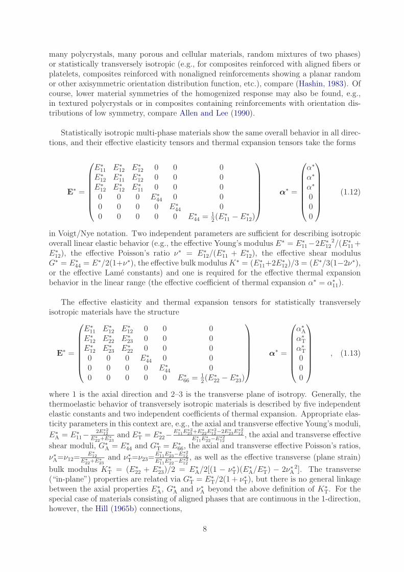
Statistically isotropic multi-phase materials show the same overall behavior in all direc-tions, and their effective elasticity tensors and thermal expansion tensors take the forms

E∗ =

E∗11 E∗

12 E∗12 0 0 0

E∗12 E∗

11 E∗12 0 0 0

E∗12 E∗

12 E∗11 0 0 0

0 0 0 E∗44 0 0

0 0 0 0 E∗44 0

0 0 0 0 0 E∗44 = 1

2(E∗

11 − E∗12)

α∗ =

α∗

α∗

α∗

000

(1.12)

in Voigt/Nye notation. Two independent parameters are sufficient for describing isotropicoverall linear elastic behavior (e.g., the effective Young’s modulus E∗ = E∗

11−2E∗12

2/(E∗11+

E∗12), the effective Poisson’s ratio ν∗ = E∗

12/(E∗11 + E∗

12), the effective shear modulusG∗ = E∗

44 = E∗/2(1+ν∗), the effective bulk modulus K∗ = (E∗11+2E∗

12)/3 = (E∗/3(1−2ν∗),or the effective Lame constants) and one is required for the effective thermal expansionbehavior in the linear range (the effective coefficient of thermal expansion α∗ = α∗

11).

The effective elasticity and thermal expansion tensors for statistically transverselyisotropic materials have the structure

E∗ =

E∗11 E∗

12 E∗12 0 0 0

E∗12 E∗

22 E∗23 0 0 0

E∗12 E∗

23 E∗22 0 0 0

0 0 0 E∗44 0 0

0 0 0 0 E∗44 0

0 0 0 0 0 E∗66 = 1

2(E∗

22 − E∗23)

α∗ =

α∗A

α∗T

α∗T

000

, (1.13)

where 1 is the axial direction and 2–3 is the transverse plane of isotropy. Generally, thethermoelastic behavior of transversely isotropic materials is described by five independentelastic constants and two independent coefficients of thermal expansion. Appropriate elas-ticity parameters in this context are, e.g., the axial and transverse effective Young’s moduli,

E∗A = E∗

11− 2E∗212

E∗

22+E∗

23and E∗

T = E∗22− E∗

11E∗223+E∗

22E∗212−2E∗

23E∗212

E∗

11E∗

22−E∗212

, the axial and transverse effective

shear moduli, G∗A = E∗

44 and G∗T = E∗

66, the axial and transverse effective Poisson’s ratios,

ν∗A=ν12=E∗

12

E∗

22+E∗

23and ν∗T=ν23=

E∗

11E∗

23−E∗212

E∗

11E∗

22−E∗212

, as well as the effective transverse (plane strain)

bulk modulus K∗T = (E∗

22 + E∗23)/2 = E∗

A/2[(1 − ν∗T)(E∗A/E

∗T) − 2ν∗A

2]. The transverse(“in-plane”) properties are related via G∗

T = E∗T/2(1 + ν∗T), but there is no general linkage

between the axial properties E∗A, G∗

A and ν∗A beyond the above definition of K∗T. For the

special case of materials consisting of aligned phases that are continuous in the 1-direction,however, the Hill (1965b) connections,

8

E∗A = ξE

(f)A + (1− ξ)E(m) +

4(ν(f)A − ν(m))2

(1/K(f)T − 1/K

(m)T )2

(ξ

K(f)T

+1− ξK

(m)T

− 1

K∗T

)

ν∗A = ξν(f)A + (1− ξ)ν(m) +

ν(f)A − ν(m)

1/K(f)T − 1/K

(m)T

(ξ

K(f)T

+1− ξK

(m)T

− 1

K∗T

), (1.14)

allow the effective moduli E∗A and ν∗A to be expressed by K∗

T, some constituent properties,and the fiber volume fraction ξ = Ω(f)/Ω; see also Milton (2002). Analogous relations holdfor unidirectionally reinforced composites of tetragonal macroscopic symmetry (Berggrenet al., 2003). Both an axial and a transverse effective coefficient of thermal expansion,α∗A = α∗

11 and α∗T = α∗

22, are required for transversely isotropic materials.

The overall material symmetries of inhomogeneous materials and their effect on var-ious physical properties can be treated in full analogy to the symmetries of crystals asdiscussed, e.g., by Nye (1957). Accordingly, deviations of predicted elastic tensors frommacroscopically isotropic elastic symmetry can be assessed via a Zener (1948) anisotropyratio, Z = 2E∗

66/(E∗22−E∗

23), or other anisotropy parameters, see, e.g., Kanit et al. (2006).

The influence of the overall symmetry of the phase arrangement on the overall me-chanical behavior of inhomogeneous materials can be marked10, especially in the case ofthe nonlinear responses to mechanical loads. Accordingly, it is good practice to aim atapproximating the symmetry of the actual material as closely as possible in any modelingeffort.

1.5 Major Modeling Strategies in Continuum Micro-

mechanics of Materials

All micromechanical methods described in the present report can be used to carry out ma-terials characterization, i.e., simulating the overall material response under simple loadingconditions such as uniaxial tensile tests. Many homogenization procedures can also be em-ployed directly to provide micromechanically based constitutive material models at higherlength scales. This implies that they allow evaluating the full homogenized stress andstrain tensors for any pertinent loading condition and for any pertinent loading history11.This task is obviously much more demanding than materials characterization. Comparedto semi-empirical constitutive laws, as proposed, e.g., by Davis (1996), micromechanically

10Overall properties described by tensors or lower rank, e.g., thermal expansion and thermal conduction,are less sensitive to material symmetry effects than are mechanical responses, compare Nye (1957).

11The overall thermomechanical behavior of homogenized materials is often richer than that of theconstituents, i.e., the effects of the interaction of the constituents in many cases cannot be satisfactorilydescribed by simply adapting material parameters without changing the functional relationships in theconstitutive laws of the constituents. For example, a composite consisting of a matrix that follows J2plasticity and elastic reinforcements shows some pressure dependence in its macroscopic plastic behavior,and the macroscopic flow behavior of inhomogeneous materials can lose normality even though that ofeach of the constituents is associated (Li and Ostoja-Starzewski, 2006). Also, two dissimilar constituentsfollowing Maxwell-type linear viscoelastic behavior do not necessarily give rise to a macroscopic Maxwellbehavior (Barello and Levesque, 2008).

9

based constitutive models have both a clear physical basis and an inherent capability for“zooming in” on the local phase stresses and strains by using localization procedures.

Evaluating the local responses of the constituents (in the ideal case, at any materialpoint) for a given macroscopic state of a sample or structure, i.e., localization, is of specialinterest for identifying local deformation mechanisms and for studying as well as assessinglocal strength relevant behavior, such as the onset and progress of plastic yielding or ofdamage, which, of course, can have major repercussions on the macroscopic behavior. Forvalid descriptions of local strength-relevant responses details of the microgeometry tend tobe of major importance and may, in fact, determine the macroscopic response, an extremecase being the mechanical strength of brittle inhomogeneous materials.

Because for realistic phase distributions an exact analysis of the spatial variations of themicrofields in large volume elements tends to be beyond present capabilities12 suitable ap-proximations must be introduced. For convenience, the majority of the resulting modelingapproaches may be treated as falling into two groups. The first of these comprises methodsthat describe interactions, e.g., between phases or between individual reinforcements, in acollective way, its main representatives being

• Mean-Field Approaches (MFAs) and related methods (see chapter 2): Highly ideal-ized microgeometries are used (compare, e.g., fig 2.1) and the microfields within eachconstituent are approximated by their phase averages 〈ε〉(p) and 〈σ〉(p), i.e., phase-wise uniform stress and strain fields are employed. The phase geometry enters thesemodels, sometimes implicitly, via statistical descriptors, such as volume fractions,macroscopic symmetry, phase topology, reinforcement aspect ratios, etc. In MFAsthe localization relations take the form

〈ε〉(p) = A(p)〈ε〉〈σ〉(p) = B(p)〈σ〉 (1.15)

and the homogenization relations can be written as

〈ε〉(p) =1

Ω(p)

∫

Ω(p)

ε(x) dΩ with 〈ε〉 =∑

pV (p)〈ε〉(p)

〈σ〉(p) =1

Ω(p)

∫

Ω(p)

σ(x) dΩ with 〈σ〉 =∑

pV (p)〈σ〉(p) , (1.16)

where (p) denotes a given phase of the material, Ω(p) is the volume occupied by thisphase, and V (p)=Ω(p)/

∑k Ω(k)=Ω(p)/Ωs is the volume fraction of the phase. In contrast

to eqn. (1.5) the phase concentration tensors A and B used in MFAs are not functionsof the spatial coordinates13.Mean-field approaches tend to be formulated (and provide estimates for effectiveproperties) in terms of the phase concentration tensors, they pose low computationalrequirements, and they have been highly successful in describing the thermoelastic

12Exact predictions of the effective properties would require an infinite set of correlation functions forstatistically characterizing the inhomogeneous microstructure, compare Torquato et al. (1999).

13Surface integral formulations analogous to eqn. (1.4) may be used to evaluate consistent expressionsfor 〈ε〉(p) for void-like and 〈σ〉(p) for rigid inhomogeneities embedded in a matrix.

10

response of inhomogeneous materials. Their use in modeling nonlinear compositescontinues to be a subject of active research. Their most important representativesare effective field and effective medium approximations.

• Bounding Methods (see chapter 3): Variational principles are used to obtain upperand (in many cases) lower bounds on the overall elastic tensors, elastic moduli, secantmoduli, and other physical properties of inhomogeneous materials the microgeome-tries of which are described by statistical parameters. Many analytical bounds areobtained on the basis of phase-wise constant stress polarization fields, making themclosely related to MFAs. Bounds — in addition to their intrinsic value — are tools ofvital importance in assessing other models of inhomogeneous materials. Furthermore,in most cases one of the bounds provides useful estimates for the physical propertyunder consideration, even if the bounds are rather slack (Torquato, 1991).

Because they do not explicitly account for pair-wise or multi-particle interactions mean-field approaches have sometimes been referred to as “non-interacting approximations” inthe literature. This designator, however, is best limited to the dilute regime in the senseof section 2.2, collective interactions being explicitly incorporated into mean-field modelsfor non-dilute volume fractions. MFA and bounding methods implicitly postulate the ex-istence of a representative volume element.

The second group of approximations are based on studying discrete microgeometries,for which they aim at evaluating the microfields at high resolution, thus fully accountingfor the interactions between phases within the “simulation box”. It includes the followinggroups of models, compare the sketches in fig. 1.1.

• Periodic Microfield Approaches (PMAs), often referred to as periodic homogenizationschemes and sometimes as unit cell methods, see chapter 5. In such models the inho-mogeneous material is approximated by an infinitely extended model material witha periodic phase arrangement. The resulting periodic microfields are usually evalu-ated by analyzing a repeating volume element (which may describe microgeometriesranging from rather simplistic to highly complex ones) via analytical or numericalmethods. Such approaches are often used for performing materials characterizationof inhomogeneous materials in the nonlinear range, but they can also be employed asmicromechanically based constitutive models. The high resolution of the microfieldsprovided by PMAs can be very useful in studying the initiation of damage at themicroscale. However, because they inherently give rise to periodic configurations ofdamage and patterns of cracks, PMAs typically are not a good choice for investi-gating phenomena such as the interaction of the microgeometry with macroscopiccracks.Periodic microfield approaches can give detailed information on the local stress andstrain fields within a given unit cell, but they tend to be relatively expensive com-putationally. Among the methods in this group they are the only one that does notintrinsically give rise to boundary layers in the microfields.

• Windowing Approaches (see chapter 6): Subregions (“windows”) — usually, butnot necessarily, of rectangular or hexahedral shape — are randomly chosen froma given phase arrangement and subjected to boundary conditions that guarantee

11

energy equivalence between the micro- and macroscales. Accordingly, windowingmethods describe the behavior of individual inhomogeneous samples rather than ofinhomogeneous materials and typically give rise to apparent rather than effectivemacroscopic responses. For the special cases of macrohomogeneous stress and strainboundary conditions, respectively, lower and upper estimates for and bounds on theoverall behavior of the inhomogeneous material can be obtained. In addition, mixedhomogeneous boundary conditions can be applied in order to generate estimates.

• Embedded Cell or Embedding Approaches (ECAs; see chapter 7): The inhomoge-neous material is approximated by a model consisting of a “core” containing a discretephase arrangement that is embedded within some outer region showing smeared-outmaterial behavior; far field loads are applied to this outer region. The material prop-erties of the embedding layer may be described by some macroscopic constitutive law,they can be determined self-consistently or quasi-self-consistently from the behaviorof the core, or the embedding region may take the form of a coarse description and/ordiscretization of the phase arrangement. ECAs can be used for materials character-ization, and they are usually the best choice for studying regions of special interestin inhomogeneous materials, such as the surroundings of tips of macroscopic cracks.Like PMAs, embedded cell approaches can resolve local stress and strain fields in thecore region at high detail, but tend to be computationally expensive.

• Other homogenization approaches employing discrete microgeometries, such as sub-modeling techniques (on which some remarks are given in chapter 7), or the statistics-based non-periodic homogenization scheme of Li and Cui (2005).

Because the above group of methods explicitly study mesodomains as defined by Hashin(1983) they are sometimes referred to as “mesoscale approaches”, and because the mi-crofields are evaluated at a high level of detail, the name “full field models” is often used.Figure 1.1 shows a sketch of a volume element as well as PMA, ECA and windowing ap-proaches applied to it.

Some further descriptions that have been applied to studying the macroscopic thermo-mechanical behavior of inhomogeneous materials, such as isostrain and isostress models(the former being known as the “rules of mixture”) and the Halpin–Tsai equations14 arenot discussed here because, with the exception of special cases, their connection to ac-tual microgeometries is not very strong, limiting their predictive capabilities. For brevity,a number of micromechanical models with solid physical basis, such as expressions forself-similar composite sphere assemblages (CSA, Hashin (1962)) and composite cylinderassemblages (CCA, Hashin and Rosen (1964)), are not covered within the present discus-sion, either.

14For certain moduli of composites reinforced by particles or by continuous aligned fibers the Halpin–Tsai equations can be obtained from the estimates of Kerner (1956) and Hermans (1967), respectively.Following the procedures outlined in Halpin and Kardos (1976) these models, together with Hill’s con-nections, eqns. (1.14), and some minor approximations, yield sets of specific “Halpin–Tsai-parameters”which, however, do not appear to have been used widely in practice. In most cases, instead, the Halpin–Tsai equations were applied in a semi-empirical way to other moduli or to other composite geometries, orwere used with other sets of parameters of various provenience.

12

PERIODIC APPROXIMATION,PHASE ARRANGEMENTUNIT CELL

EMBEDDED CONFIGURATION WINDOW

Figure 1.1: Schematic sketch of a random matrix–inclusion microstructure and of the volume ele-ments used by a periodic microfield method (which employs a slightly different periodic “model”microstructure), an embedding scheme and a windowing approach to studying this inhomoge-neous material.

For studying materials that are inhomogeneous at a number of (sufficiently widelyspread) length scales (e.g., materials in which well defined clusters of inhomogeneities arepresent), hierarchical procedures that use homogenization at more than one level are anatural extension of the above concepts. Such multi-scale or sequential homogenizationmodels are the subject of a short discussion in chapter 8.

A final group of models used for studying inhomogeneous materials is the direct numer-ical simulation (DNS) of microstructured structures or samples. Until recently, approachesdescribing full inhomogeneous configurations were restricted to models the size of which ex-ceeds the microscale by less than, say, one or two orders of magnitude, see, e.g., Papka andKyriakides (1994), Silberschmidt and Werner (2001), Luxner et al. (2005) or Tekoglu et al.(2011). Even though such geometries may appear similar to the ones used in windowing ap-proaches, compare chapter 6, such models by design aim at describing the behavior of smallstructures rather than that of a material. As a consequence, they are typically subjectedto boundary conditions and load cases that are more pertinent to structures (among thembending or indentation loads) than to materials. The effects of these boundary conditionsas well as the sample’s size in terms of the characteristic length of the inhomogeneities

13

typically play considerable roles in the mechanical behavior of such inhomogeneous bodies,which is often evaluated in terms of force vs. displacement rather than stress vs. straincurves. Recent improvements in computing power have allowed extending DNS models tolarger structures, compare, e.g., Bishop et al. (2015). Arguably, such structural modelsare not part of the “core tool set” of micromechanics, because they do not involve scaletransitions.

1.6 Model Verification and Validation

Micromechanical approaches aim at generating predictive models for the behavior of in-homogeneous materials. Obviously, model verification, i.e., monitoring a model’s correctsetup and implementation, as well as validation, i.e., assessing the accuracy of a model’srepresentation of the targeted material behavior, play important roles in this context. Ofcourse, both model verification and validation in continuum micromechanics require keep-ing tabs on the consistency and plausibility of modeling assumptions and results throughouta given study.

For verification, it is often possible to compare predictions obtained with different, un-related micromechanical methods that pertain to a given geometrical configuration andemploy the same constitutive models as well as material parameters. Bounding meth-ods, see chapter 3, play an especially important role in this respect; When it comes tostudying the linear elastic (or conduction) responses of inhomogeneous materials, in manycases appropriate bounds are available, compare section 3. Analytical or numerical modelsthat violate the Hashin–Shtrikman bounds pertaining to the macroscopic symmetry andmicroscopic geometrical configuration of the material in the linear regime by more thantrivial differences (which may be due to, e.g., roundoff errors), must be viewed as flawed15.In such verification assessments the value of an estimate relative to the pertinent boundsmay provide additional information, stiff inhomogeneities in a compliant matrix giving riseto effective moduli closer to the lower and compliant inhomogeneities in a stiff matrix toestimates closer to the upper bound (Torquato, 1991); analogous relationships hold forconduction problems. It is good practice to assess linear versions of models intended forstudying nonlinear behavior against the appropriate bounds — this essentially provides acheck if a given model produces a physically vali partitioning of the stress (flux) and strain(gradient) fields between the target material’s phases. Issues cropping up with linear be-havior tend not to disappear, but rather to become more marked in the more complexnonlinear setting.

In the case of modeling efforts making use of discretizing numerical engineering methodsfor evaluating position dependent fields in a volume element, convergence studies involvingsuccessively finer discretizations are an important part of verification. In this context it isworth noting that convergence in terms of the macroscopic responses does not guaranteeconvergence in terms of the microscopic fields, and, especially, of the latters’ minumumand maximum values.

15If data from measurements do not comply with the pertinent Hashin–Shtrikman bounds the mostcommon reason is inaccurate data for the constituent behavior or volume fractions. Measurement errorsmay, however, also play a role.

14

The validation of micromechanical models against experimental data is obviously highlyimportant, but may be tricky in practice due to the considerable number of potentialsources of discrepancies — among them are the representativeness of the volume elements,the quality of the material models used for the constituents, the accuracy of the materialparameters used with these constitutive models, as well as experimental inaccuracies. Ob-taining perfect or near-perfect agreement between measurements and predictions without“tuning” input parameters in general is not the most probable of outcomes, especially whendamage and failure modeling are involved. Accordingly, even highly successful validationagainst experimental data does not remove the need for model verification as defined above.Specifically, a model giving predictions that are close to experimental results but fall out-side the pertinent bounds in the linear range cannot be treated as verified — after all, evengood agreement with measurements may be due to the canceling of different errors arisingfrom the above issues. In a similar vein, obtaining responses close to experimental resultsfrom a model that takes major liberties in terms of the microgeometry constitutes neitherverification nor proper validation.

Obtaining reliable values for material parameters pertinent to the microscale tends tobe a major challenge in micromechanics, especially when a model involves damage. Afairly common way of dealing with this problem is carrying out parameter identificationvia inverse procedures built around the micromechanical model and available experimentalresults. When following such a strategy, using the same set of experimental data forboth parameter identification and model verification must be avoided — in such a setting“overspecialization” of the parameters to that data set may occur, which makes model andparameters unsuitable for generalization to other situations. In a common scenario of thistype the nonlinear macroscopic behavior of a composite is to be studied and experimentaldata are limited to results from uniaxial tensile tests. In such a case even a perfect matchof predictions with the above experimental results is far from guaranteeing that load casesinvolving other macroscopic triaxialities, e.g., shear, or complex stress trajectories will bedescribed reasonably well by the model.

15

Chapter 2

Mean-Field Methods

In this chapter mean-field relations are discussed mainly for two-phase materials, exten-sions to multi-phase materials being fairly straightforward in many cases. Special emphasisis put on effective field methods of the Mori–Tanaka type, which may be viewed as thesimplest mean-field approaches to modeling inhomogeneous materials that encompass thefull physical range of phase volume fractions16. Unless specifically stated otherwise, thematerial behavior of both reinforcements and matrix is taken to be linear (thermo)elastic,both strains and temperature changes being assumed to be small. Perfect bonding betweenthe constituents is assumed in all cases. There is an extensive body of literature coveringmean-field approaches, so that the following treatment is far from complete.

2.1 General Relations between Mean Fields in Thermo-

elastic Two-Phase Materials

Throughout this report additive decomposition of strains is used. For example, for thecase of thermoelastoplastic material behavior the total strain tensor can be written in thisapproximation as

ε = εel + εpl + εth , (2.1)

where εel, εpl and εth denote the elastic, plastic and thermal strains, respectively. The strainand stress tensors may be split into volumetric/hydrostatic and deviatoric contributions

ε = εvol + εdev = Ovol ε + Odev ε

σ = σhyd + σdev = Ovol σ + Odev σ , (2.2)

Ovol and Odev being volumetric and deviatoric projection tensors.

For thermoelastic inhomogeneous materials, the macroscopic stress–strain relations canbe written in the form

〈σ〉 = E∗〈ε〉+ λ∗∆T

〈ε〉 = C∗〈σ〉+ α∗∆T . (2.3)

16Because Eshelby and Mori–Tanaka methods are specifically suited for matrix–inclusion-type micro-topologies, the expression “composite” is often used in the present chapter instead of the more generaldesignation “inhomogeneous material”.

16

Here the expression α∗∆T corresponds to the macroscopic thermal strain tensor, λ∗ =−E∗α∗ is the macroscopic specific thermal stress tensor (i.e., the overall stress responseof a fully constrained material to a purely thermal unit load, also known as the tensor ofthermal stress coefficients), and ∆T stands for the (spatially homogeneous) temperaturedifference with respect to some (stress-free) reference temperature. The constituents, herea matrix (m) and inhomogeneities (i), are also assumed to behave thermoelastically, so that

〈σ〉(m) = E(m)〈ε〉(m) + λ(m)∆T 〈σ〉(i) = E(i)〈ε〉(i) + λ(i)∆T

〈ε〉(m) = C(m)〈σ〉(m) + α(m)∆T 〈ε〉(i) = C(i)〈σ〉(i) + α(i)∆T , (2.4)

where the relations λ(m) = −E(m)α(m) and λ(i) = −E(i)α(i) hold.

From the definition of phase averaging, eqn. (1.16), relations between the phase aver-aged fields in the form

〈ε〉 = ξ〈ε〉(i) + (1− ξ)〈ε〉(m) = εa

〈σ〉 = ξ〈σ〉(i) + (1− ξ)〈σ〉(m) = σa (2.5)

follow immediately, where ξ = V (i) = Ω(i)/Ωs stands for the volume fraction of the re-inforcements and 1 − ξ = V (m) = Ω(m)/Ωs for the volume fraction of the matrix. εa andσa denote far field (“applied”) homogeneous stress and strain tensors, respectively, withεa = C∗σa. Perfect interfaces between the phases are assumed in expressing the macro-scopic strain of the composite as the weighted sum of the phase averaged strains.

The phase averaged strains and stresses can be related to the overall strains and stressesby the phase averaged strain and stress concentration (or localization) tensors A, β, B, andκ (Hill, 1963), respectively, which are defined for thermoelastic inhomogeneous materialsby the expressions

〈ε〉(m) = A(m)〈ε〉+ β(m)

∆T 〈ε〉(i) = A(i)〈ε〉+ β(i)

∆T

〈σ〉(m) = B(m)〈σ〉+ κ(m)∆T 〈σ〉(i) = B(i)〈σ〉+ κ(i)∆T , (2.6)

compare eqn. (1.15) for the purely elastic case. A and B are referred to as the mechanicalor (elastic) phase stress and strain concentration tensors, respectively, and β as well as κ

are the corresponding thermal concentration tensors.

By using eqns. (2.5) and (2.6), the strain and stress concentration tensors can be shownto fulfill the relations

ξA(i) + (1− ξ)A(m) = I ξβ(i)

+ (1− ξ)β(m)= o

ξB(i) + (1− ξ)B(m) = I ξκ(i) + (1− ξ)κ(m) = o , (2.7)

where I stands for the symmetric rank 4 identity tensor and o for the rank 2 null tensor.

The effective elasticity and compliance tensors of a two-phase composite can be obtainedfrom the properties of the constituents and from the mechanical concentration tensors as

E∗ = ξE(i)A(i) + (1− ξ)E(m)A(m)

= E(m) + ξ[E(i) − E(m)]A(i) = E(i) + (1− ξ)[E(m) − E(i)]A(m) (2.8)

17

C∗ = ξC(i)B(i) + (1− ξ)C(m)B(m)

= C(m) + ξ[C(i) −C(m)]B(i) = C(i) + (1− ξ)[C(m) −C(i)]B(m) , (2.9)

compare eqn. (1.11). For multi-phase materials with N phases (p) the equivalents ofeqn. (2.7) take the form

∑

(p)

ξ(p)A(p) = I∑

(p)

ξ(p)β(p)

= o

∑

(p)

ξ(p)B(p) = I∑

(p)

ξ(p)κ(p) = o , (2.10)

and the effective elastic tensors can be evaluated as

E∗ =∑

(p)

ξ(p)E(p)A(p) C∗ =∑

(p)

ξ(p)C(p)B(p) (2.11)

by analogy to eqns. (2.8) and (2.9).The tensor of effective thermal expansion coefficients, α∗, and the specific thermal

stress tensor, λ∗, can be related to the thermoelastic phase behavior and the thermalconcentration tensors as

α∗ = ξ[C(i)κ(i) + α(i)] + (1− ξ)[C(m)κ(m) + α(m)]

= ξα(i) + (1− ξ)α(m) + (1− ξ)[C(m) −C(i)]κ(m)

= ξα(i) + (1− ξ)α(m) + ξ[C(i) −C(m)]κ(i) . (2.12)

λ∗ = ξ[E(i)β(i)

+ λ(i)] + (1− ξ)[E(m)β(m)

+ λ(m)]

= ξλ(i) + (1− ξ)λ(m) + (1− ξ)[E(m) − E(i)]β(m)

= ξλ(i) + (1− ξ)λ(m) + ξ[E(i) − E(m)]β(i)

. (2.13)

The above expressions can be derived by inserting eqns. (2.4) and (2.6) into eqns. (2.5)and comparing with eqns. (2.3). Alternatively, the effective thermal expansion coefficientand specific thermal stress coefficient tensors of multi-phase materials can be obtained as

α∗ =∑

(p)

ξ(p)(B(p))Tα(p)

λ∗ =∑

(p)

ξ(p)(A(p))Tλ(p) , (2.14)

compare (Mandel, 1965; Levin, 1967), the expression for α∗ being known as the Mandel–Levin formula. If the effective compliance tensor of a two-phase material is known,eqn. (2.7) can be inserted into eqn. (2.14) to give the overall coefficients of thermal expan-sion as

α∗ = (C∗ −C(m))(C(i) −C(m))−1α(i) − (C∗ −C(i))(C(i) −C(m))−1α(m) . (2.15)

The mechanical stress and strain concentration tensors for a given phase are linked byexpressions of the type

A(p) = C(p)B(p)E∗ and B(p) = E(p)A(p)C∗ , (2.16)

18

from which E∗ and C∗ may be eliminated via eqn. (2.11) to give

A(p) = C(p)B(p)[∑

(q)

ξ(q)C(q)B(q)]−1

and B(p) = E(p)A(p)[∑

(q)

ξ(q)E(q)A(q)]−1

, (2.17)

respectively. By invoking the principle of virtual work additional relations were devel-oped (Benveniste and Dvorak, 1990; Benveniste et al., 1991) which link the thermal strain

concentration tensors, β(p)

, to the mechanical strain concentration tensors, A(p), and thethermal stress concentration tensors, κ(p), to the mechanical stress concentration tensors,B(p), respectively, as

β(m)

= [I− A(m)][E(i) − E(m)]−1[λ(m) − λ(i)]

β(i)

= [I− A(i)][E(m) − E(i)]−1[λ(i) − λ(m)]

κ(m) = [I− B(m)][C(i) −C(m)]−1[α(m) −α(i)]

κ(i) = [I− B(i)][C(m) −C(i)]−1[α(i) −α(m)] . (2.18)

From eqns. (2.9) to (2.18) it is evident that the knowledge of one elastic phase con-centration tensor is sufficient for describing the full thermoelastic behavior of a two-phaseinhomogeneous material within the mean-field framework17. A fair number of additionalrelations between phase averaged tensors have been given in the literature.

An additional set of concentration tensors, useful for describing inhomogeneous materi-als with matrix–inclusion topology, are the partial strain and stress concentration tensors,T(i) and W(i), defined by the expressions

ε(i) = T(i)ε(m)

σ(i) = W(i)σ(m) , (2.19)

compare, e.g., Dvorak and Benveniste (1992). These partial concentration tensors arelinked to the phase concentration tensors by the relations

A(m) =[ξT(i) + (1− ξ)I

]−1

B(m) =[ξW(i) + (1− ξ)I

]−1

A(i) = T(i)[ξT(i) + (1− ξ)I

]−1

B(i) = W(i)[ξW(i) + (1− ξ)I

]−1. (2.20)

The inverse of the partial inhomogeneity stress concentration tensor, [W(i)]−1 is sometimesreferred to as the “bridging tensor”, see Huang (2000).

Equations (2.3) to (2.18) do not account for temperature dependence of the thermoe-lastic moduli. For a mean-field framework capable of handling temperature dependentmoduli for finite temperature excursions and small strains see, e.g., Boussaa (2011).

17Similarly, n−1 of either the elastic strain or stress phase concentration tensors must be known forevaluating the overall elastic behavior of an n-phase material. In general, however, additional data isrequired for evaluating the thermal concentration tensors for n > 3.

19

2.2 Eshelby Tensor and Dilute Matrix–Inclusion Com-

posites

Eshelby’s Eigenstrain Problem

A large percentage of the mean-field descriptions used in continuum micromechanics ofmaterials have been based on the work of Eshelby, who initially studied the stress andstrain distributions in homogeneous media that contain a subregion (“inclusion”) thatspontaneously changes its shape and/or size (“undergoes a transformation”) so that it nolonger fits into its previous space in the “parent medium”. Eshelby’s results show that if anelastic homogeneous ellipsoidal inclusion (i.e., an inclusion consisting of the same materialas the matrix) in an infinite matrix is subjected to a homogeneous strain εt (called the“stress-free strain”, “unconstrained strain”, “eigenstrain”, or “transformation strain”), thestress and strain states in the constrained inclusion are uniform18, i.e., σ(i) = 〈σ〉(i) andε(i) = 〈ε〉(i). The uniform strain in the constrained inclusion (the “constrained strain”),ε(i) = εc, is related to the stress-free strain εt by the expression (Eshelby, 1957)

εc = Sεt , (2.21)

where S is referred to as the (interior point) Eshelby tensor. For eqn. (2.21) to hold, εtmay be any kind of eigenstrain that is uniform over the inclusion (e.g., a thermal strain ora strain due to some phase transformation involving no changes in the elastic constants ofthe inclusion).

The Eshelby tensor S depends only on the material properties of the “parent medium”(often the matrix) and on the specific shape of the ellipsoidal inclusions. Eshelby tensorsfor inclusions of general shape can be obtained as

S(x) =

∫

Ω(i)

G(0)(x− x′)E(0) dΩ′ = P(0)(x)E(0) , (2.22)

compare, e.g., Kachanov and Sevostianov (2018). Here G(0) and E(0) stand for the modifiedGreen’s tensor and the elasticity tensor of the parent medium (0), respectively, and P(0) isknown as the Hill tensor, mean polarization factor tensor or shape tensor. The so-calledfirst Eshelby problem consists in finding solutions for the above integral.

Closed form expressions for the Eshelby tensor of spheroidal inclusions in an isotropicmatrix are available as functions of the aspect ratio (eccentricity) a, see, e.g., Pedersen(1983), Tandon and Weng (1984), Mura (1987) or Clyne and Withers (1993), the formu-lae resulting for continuous fibers of circular cross-section (a → ∞), spherical inclusions(a = 1), and thin circular disks or layers (a → 0) being rather simple. Analogous expres-sions for the Eshelby tensor have also been reported for spheroidal inclusions in a matrix oftransversely isotropic material symmetry (Withers, 1989; Parnell and Calvo-Jurado, 2015),provided the material axes of the matrix are aligned with the orientations of non-spherical

18This “Eshelby property” or “Eshelby uniformity” is limited to inclusions and inhomogeneities of ellip-soidal shape (Lubarda and Markenscoff, 1998; Kang and Milton, 2008). However, hyperboloidal domainswill (Franciosi, 2020) and certain non-dilute periodic arrangements of non-ellipsoidal inclusions can (Liuet al., 2007) also give rise to homogeneous fields.

20

inclusions. Expressions for the Eshelby tensors of ellipsoidal inclusions in an isotropicmatrix in terms of incomplete elliptic integrals (which, in general, must be evaluated nu-merically) can be found, e.g., in Mura (1987). Instead of evaluating the Eshelby tensor fora given configuration, the Hill tensor P(0), may be solved for instead, compare, e.g., PonteCastaneda (1996) or Masson (2008). For detailed discussion of Eshelby and Hill tensorspertaining to ellipsoidal inclusions see Parnell (2016); information on position-dependentand averaged Eshelby tensors for polyhedral inhomogeneities embedded in an isotropicmatrix is provided, e.g., by Kachanov and Sevostianov (2018).

For materials of low elastic symmetry the modified Green’s function tensor G(0) asrequired in eqn. (2.22) is not available. However, the problem can be transformed intoa surface integral in Fourier space (Mura, 1987), where the modified Green’s tensors areknown explicitly for all symmetries. On this basis, approximations to the Eshelby tensorsof ellipsoids embedded in a matrix of general elastic symmetry can be obtained by numer-ical quadrature, compare Gavazzi and Lagoudas (1990).

Eshelby’s Inhomogeneity Problem

For mean-field descriptions of dilute matrix–inclusion composites, the main interest lieson the stress and strain fields in inhomogeneous inclusions (“inhomogeneities”) that areembedded in a matrix and that do not interact with each other. Such cases can be handledon the basis of Eshelby’s theory for homogeneous inclusions, eqn. (2.21), by introducingthe concept of an equivalent homogeneous inclusion. This strategy involves replacing anactual perfectly bonded inhomogeneity, which has different material properties than thematrix and which is subjected to a given unconstrained eigenstrain εt, with a (fictitious)“equivalent” homogeneous inclusion on which a (fictitious) “equivalent” eigenstrain ετ ismade to act. This equivalent eigenstrain must be chosen in such a way that the inhomo-geneous inclusion and the equivalent homogeneous inclusion attain the same stress stateσ(i) and the same constrained strain εc (Eshelby, 1957; Withers et al., 1989). When σ(i)

is expressed in terms of the elastic strain in the inhomogeneity or inclusion, this conditiontranslates into the equality

σ(i) = E(i)[εc − εt] = E(m)[εc − ετ ] . (2.23)

Here εc − εt and εc − ετ are the elastic strains in the inhomogeneous inclusion and theequivalent homogeneous inclusion, respectively. Obviously, in the general case the stress-free strains will be different for the equivalent inclusion and the real inhomogeneity, εt 6= ετ .Plugging the result of applying eqn. (2.21) to the equivalent eigenstrain, εc = Sετ , intoeqn. (2.23) leads to the relationship

σ(i) = E(i)[Sετ − εt] = E(m)[S− I]ετ , (2.24)

which can be rearranged to obtain the equivalent eigenstrain as a function of the knownstress-free eigenstrain εt of the inhomogeneous inclusion as

ετ = [(E(i) − E(m))S + E(m)]−1E(i)εt . (2.25)

This, in turn, allows the stress in the inhomogeneity, σ(i), to be expressed as

σ(i) = E(m)(S− I)[(E(i) − E(m))S + E(m)]−1E(i)εt . (2.26)

21

The concept of the equivalent homogeneous inclusion can be extended to the “inho-mogeneity problem”, where a uniform mechanical strain εa or stress σa is applied to asystem consisting of a perfectly bonded inhomogeneous elastic inclusion in an infinite ma-trix. Here, the strain in the inhomogeneity, ε(i), is a superposition of the applied strainand of a term εc that accounts for the constraint effects of the surrounding matrix. Well-known expressions for dilute, non-interacting elastic concentration tensors based on theabove considerations were proposed by Hill (1965c) and elaborated by Benveniste (1987).For deriving them, the conditions of equal stresses and strains in the actual inhomogeneity(elasticity tensor E(i)) and the equivalent inclusion (elasticity tensor E(m)) under an appliedfar field strain εa take the form

σ(i) = E(i)[εa + εc] = E(m)[εa + εc − ετ ] (2.27)

andε(i) = εa + εc = εa + Sετ , (2.28)

respectively, where eqn. (2.21) is used to describe the constrained strain of the equivalenthomogeneous inclusion. On the basis of these relationships the strain in the inhomogeneitycan be expressed as

ε(i) = [I + SC(m)(E(i) − E(m))]−1εa . (2.29)

Because the strain in the inhomogeneity is homogeneous, ε(i) = 〈ε〉(i), the strain concen-tration tensor for dilute inhomogeneities follows directly from eqn. (2.29) as

A(i)dil = [I + SC(m)(E(i) − E(m))]−1 . (2.30)

By using 〈ε〉(i) = C(i)〈σ〉(i) as well as εa ≅ C(m)σa, the dilute stress concentration tensorfor the inhomogeneities is found from eqn. (2.29) as

B(i)dil = E(i)[I + SC(m)(E(i) − E(m))]−1C(m)

= [I + E(m)(I− S)(C(i) −C(m))]−1 . (2.31)

In the above approach the Eshelby tensor always refers to the equivalent homogeneous in-clusion and, accordingly, it is independent of the material symmetry and elastic propertiesof the inhomogeneities.

Dilute thermal concentration tensors can be generated from eqns. (2.30) and (2.31) byusing eqns. (2.7) and (2.18). Alternative expressions for dilute mechanical and thermalinhomogeneity concentration tensors were given, e.g., by Mura (1987), Wakashima et al.(1988) and Clyne and Withers (1993). All of the above relations were derived under theassumption that the inhomogeneities are dilutely dispersed in the matrix and thus do not“feel” any effects of their neighbors (i.e., they are loaded by the unperturbed applied stressσa or applied strain εa, the so-called dilute or non-interacting case). Accordingly, the re-sulting inhomogeneity concentration tensors are independent of the reinforcement volumefraction ξ. The corresponding matrix concentration tensors can be obtained via eqns. (2.7)and, accordingly, depend on ξ.

Following, e.g., Dederichs and Zeller (1973) or Kachanov and Sevostianov (2018) thestrain field in an inhomogeneity of general shape is given by

ε(i)(x) = 〈ε〉(0) + (E(i) − E(m))

∫

V (i)

G(0)(x− x′) ε(x′) dΩ′ , (2.32)

22

an equation that pertains to expressions such as eqn. (2.29). Solutions of eqn. (2.22),i.e., Hill or Eshelby tensors, in general hold for eqn. (2.32) only if ε is constant withinthe inhomogeneity, which is the case only for ellipsoids. The integral equation (2.32) is aLippmann–Schwinger equation and describes the so-called second Eshelby problem19.

The stress and strain fields outside an inhomogeneity or a transformed homogeneousinclusion in an infinite matrix are not uniform on the microscale20 (Eshelby, 1959). Withinthe framework of mean-field approaches, which aim to link the average fields in matrix andinhomogeneities with the overall response of inhomogeneous materials, however, it is onlythe average matrix stresses and strains that are of interest. For dilute composites, suchexpressions follow directly by combining eqns. (2.30) and (2.31) with eqn. (2.7). Estimatesfor the overall elastic and thermal expansion tensors can be obtained in a straightforwardway from the dilute concentration tensors A

(i)dil and B

(i)dil by using eqns. (2.8) to (2.18); such

solutions are often referred to as the Non-Interacting Approximation (NIA). It must bekept in mind, however, that all mean-field expressions of this type are strictly valid only forvanishingly small inhomogeneity volume fractions and give reasonably dependable resultsonly for ξ ≪ 0.1.

2.3 SomeMean-Field Methods for Thermoelastic Com-

posites with Aligned Reinforcements

Models of the overall thermoelastic behavior of composites with reinforcement volumefractions of more than a few percent must explicitly account for interactions between inho-mogeneities, i.e., for the effects of all surrounding reinforcements on the stress and strainfields experienced by a given fiber or particle. Within the mean-field framework such inter-action effects as well as the concomitant perturbations of the stress and strain fields in thematrix are accounted for in a collective way via approximations that are phase-wise con-stant. Beyond such “background” effects, interactions between individual reinforcementsgive rise, on the one hand, to inhomogeneous stress and strain fields within each inhomo-geneity (intra-particle and intra-fiber fluctuations in the sense of section 1.3) as well as inthe matrix. On the other hand, they cause the levels of the average stresses and strainsin individual inhomogeneities to differ, i.e., inter-particle and inter-fiber fluctuations arepresent. Neither of these interactions and fluctuations can be resolved by mean-field meth-ods.

There are two main groups of mean-field approaches to handling non-dilute inhomo-geneity volume fractions, viz., effective field and effective medium methods, both of whichhandle interactions between inhomogeneities in a collective way. Figure 2.1 schemati-cally compares the material and loading configurations underlying non-interacting (NIA,

19Eshelby tensors in the strict sense are solutions to the integral (2.22). Tensors obtained by solving theintegral equation (2.32) and then using eqn. (2.29) to extract S coincide with the proper Eshelby tensoronly if the inhomogeneity is of ellipsoidal shape.It may be noted that Eshelby (1957) did not proceed via eqns. (2.22) and (2.32).

20The fields outside a single inclusion can be described via the exterior point Eshelby tensor, see, e.g.,Ju and Sun (1999), Meng et al. (2012) or Jin et al. (2016). From the (constant) interior point fields andthe (position dependent) exterior point fields the stress and strain jumps at the interface between inclusionand matrix can be evaluated.

23

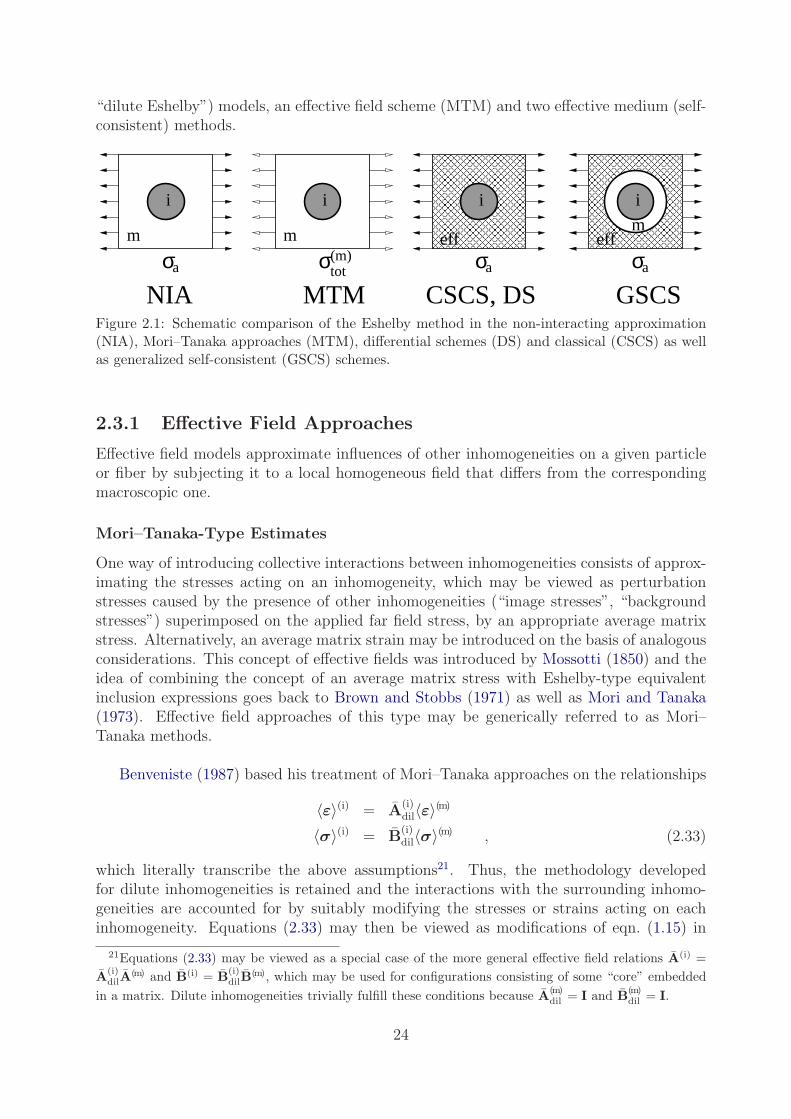
“dilute Eshelby”) models, an effective field scheme (MTM) and two effective medium (self-consistent) methods.

effeffmmm

i i i i

σ σ σσa tot a a(m)

GSCSMTMNIA CSCS, DSFigure 2.1: Schematic comparison of the Eshelby method in the non-interacting approximation(NIA), Mori–Tanaka approaches (MTM), differential schemes (DS) and classical (CSCS) as wellas generalized self-consistent (GSCS) schemes.

2.3.1 Effective Field Approaches

Effective field models approximate influences of other inhomogeneities on a given particleor fiber by subjecting it to a local homogeneous field that differs from the correspondingmacroscopic one.

Mori–Tanaka-Type Estimates

One way of introducing collective interactions between inhomogeneities consists of approx-imating the stresses acting on an inhomogeneity, which may be viewed as perturbationstresses caused by the presence of other inhomogeneities (“image stresses”, “backgroundstresses”) superimposed on the applied far field stress, by an appropriate average matrixstress. Alternatively, an average matrix strain may be introduced on the basis of analogousconsiderations. This concept of effective fields was introduced by Mossotti (1850) and theidea of combining the concept of an average matrix stress with Eshelby-type equivalentinclusion expressions goes back to Brown and Stobbs (1971) as well as Mori and Tanaka(1973). Effective field approaches of this type may be generically referred to as Mori–Tanaka methods.

Benveniste (1987) based his treatment of Mori–Tanaka approaches on the relationships

〈ε〉(i) = A(i)dil〈ε〉(m)

〈σ〉(i) = B(i)dil〈σ〉(m) , (2.33)

which literally transcribe the above assumptions21. Thus, the methodology developedfor dilute inhomogeneities is retained and the interactions with the surrounding inhomo-geneities are accounted for by suitably modifying the stresses or strains acting on eachinhomogeneity. Equations (2.33) may then be viewed as modifications of eqn. (1.15) in

21Equations (2.33) may be viewed as a special case of the more general effective field relations A(i) =

A(i)dilA

(m) and B(i) = B(i)dilB

(m), which may be used for configurations consisting of some “core” embedded

in a matrix. Dilute inhomogeneities trivially fulfill these conditions because A(m)dil = I and B

(m)dil = I.

24

which the macroscopic strain or stress, 〈ε〉 or 〈σ〉, is replaced by the phase averaged ma-trix strain or stress, 〈ε〉(m) and 〈σ〉(m), respectively.

In a further step suitable expressions for 〈ε〉(m) and/or 〈σ〉(m) must be introduced intothe scheme. This can be easily done by inserting eqn. (2.33) into eqn. (2.5), leading to therelations

〈ε〉(m) = [(1− ξ)I + ξA(i)dil]

−1〈ε〉〈σ〉(m) = [(1− ξ)I + ξB

(i)dil]

−1〈σ〉 . (2.34)

These, in turn, allow the Mori–Tanaka strain and stress concentration tensors for matrixand inhomogeneities to be written in terms of the dilute concentration tensors as

A(m)MT = [(1− ξ)I + ξA

(i)dil]

−1 A(i)MT = A

(i)dil[(1− ξ)I + ξA

(i)dil]

−1

B(m)MT = [(1− ξ)I + ξB

(i)dil]

−1 B(i)MT = B

(i)dil[(1− ξ)I + ξB

(i)dil]

−1 (2.35)

(Benveniste, 1987). Equations (2.35) may be evaluated with any strain and stress concen-

tration tensors A(i)dil and B

(i)dil pertaining to dilute inhomogeneities embedded in a matrix. If,

for example, the equivalent inclusion expressions, eqns. (2.30) and (2.31), are employed, theMori–Tanaka matrix strain and stress concentration tensors for the non-dilute compositetake the form

A(m)MT = (1− ξ)I + ξ[I + SC(m)(E(i) − E(m))]−1−1

B(m)MT = (1− ξ)I + ξE(i)[I + SC(m)(E(i) − E(m))]−1C(m)−1 , (2.36)

compare Benveniste (1987), Benveniste and Dvorak (1990) or Benveniste et al. (1991).The Mori–Tanaka approximations to the effective elastic tensors are obtained by insert-ing eqns. (2.35) and/or (2.36) into eqns. (2.8) and (2.9). By inserting eqns. (2.35) intoeqns. (2.8) the Mori–Tanaka estimates for the effective elastic tensors are obtained as

E∗MT = [ξE(i)A

(i)dil + (1− ξ)E(m)][ξA

(i)dil + I]−1

C∗MT = [ξC(i)B

(i)dil + (1− ξ)C(m)][ξB

(i)dil + I]−1 . (2.37)

A number of authors gave different but essentially equivalent Mori–Tanaka-type ex-pressions for the phase concentration tensors and effective thermoelastic tensors of inho-mogeneous materials, among them Pedersen (1983), Wakashima et al. (1988), Taya et al.(1991), Pedersen and Withers (1992) as well as Clyne and Withers (1993). Alternatively, aMori–Tanaka method can be formulated to directly give the macroscopic elasticity tensoras

E∗T = E(m)

I− ξ[(E(i) − E(m))

(S− ξ(S− I)

)+ E(m)]−1[E(i) − E(m)]

−1(2.38)

(Tandon and Weng, 1984). Because eqn. (2.38) does not explicitly use the compliancetensor of the inhomogeneities, C(i), it can be modified in a straightforward way to describethe macroscopic stiffness of porous materials by setting E(i) → 0, producing the relationship

ET,por = E(m)[I +

ξ

1− ξ (I− S)−1]−1

. (2.39)

25

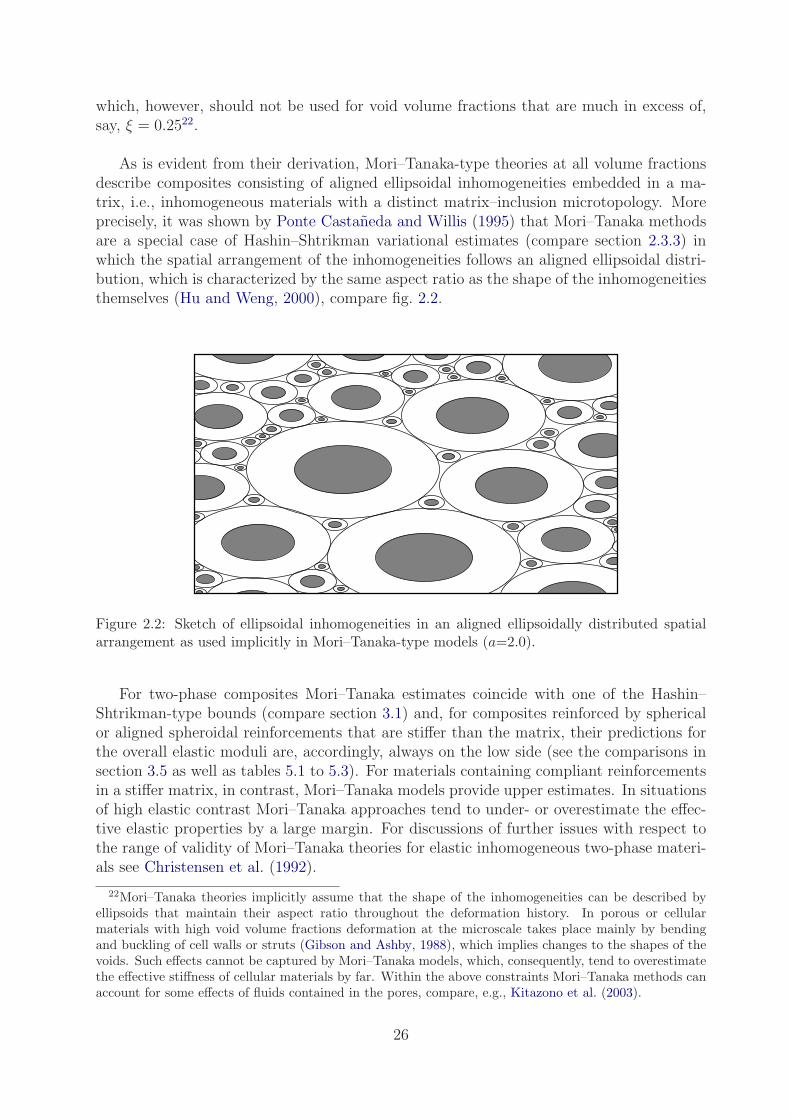
which, however, should not be used for void volume fractions that are much in excess of,say, ξ = 0.2522.

As is evident from their derivation, Mori–Tanaka-type theories at all volume fractionsdescribe composites consisting of aligned ellipsoidal inhomogeneities embedded in a ma-trix, i.e., inhomogeneous materials with a distinct matrix–inclusion microtopology. Moreprecisely, it was shown by Ponte Castaneda and Willis (1995) that Mori–Tanaka methodsare a special case of Hashin–Shtrikman variational estimates (compare section 2.3.3) inwhich the spatial arrangement of the inhomogeneities follows an aligned ellipsoidal distri-bution, which is characterized by the same aspect ratio as the shape of the inhomogeneitiesthemselves (Hu and Weng, 2000), compare fig. 2.2.

Figure 2.2: Sketch of ellipsoidal inhomogeneities in an aligned ellipsoidally distributed spatialarrangement as used implicitly in Mori–Tanaka-type models (a=2.0).

For two-phase composites Mori–Tanaka estimates coincide with one of the Hashin–Shtrikman-type bounds (compare section 3.1) and, for composites reinforced by sphericalor aligned spheroidal reinforcements that are stiffer than the matrix, their predictions forthe overall elastic moduli are, accordingly, always on the low side (see the comparisons insection 3.5 as well as tables 5.1 to 5.3). For materials containing compliant reinforcementsin a stiffer matrix, in contrast, Mori–Tanaka models provide upper estimates. In situationsof high elastic contrast Mori–Tanaka approaches tend to under- or overestimate the effec-tive elastic properties by a large margin. For discussions of further issues with respect tothe range of validity of Mori–Tanaka theories for elastic inhomogeneous two-phase materi-als see Christensen et al. (1992).

22Mori–Tanaka theories implicitly assume that the shape of the inhomogeneities can be described byellipsoids that maintain their aspect ratio throughout the deformation history. In porous or cellularmaterials with high void volume fractions deformation at the microscale takes place mainly by bendingand buckling of cell walls or struts (Gibson and Ashby, 1988), which implies changes to the shapes of thevoids. Such effects cannot be captured by Mori–Tanaka models, which, consequently, tend to overestimatethe effective stiffness of cellular materials by far. Within the above constraints Mori–Tanaka methods canaccount for some effects of fluids contained in the pores, compare, e.g., Kitazono et al. (2003).

26

For multi-phase materials consisting of a matrix (m) into which a number of alignedinhomogeneity phases (i) are embedded, extended the Mori–Tanaka phase concentrationtensors can be given as

A(m)MT =

[ξ(m)I +

∑(i) 6=(m)

ξ(i)A(i)dil

]−1A

(i)MT = A

(i)dil

[ξ(m)I +

∑

(i) 6=(m)

ξ(i)A(i)dil

]−1

B(m)MT =

[ξ(m)I +

∑(i) 6=(m)

ξ(i)B(i)dil

]−1B

(i)MT = A

(i)dil

[ξ(m)I +

∑

(j)6=(m)

ξ(i)B(i)dil

]−1(2.40)

and the macroscopic elastic tensors are obtained as

E∗MT =

[ξ(m)E(m) +

∑

(i) 6=(m)

ξ(i)E(i)A(i)dil

] [ξ(m)I +

∑

(i) 6=(m)

ξ(i)A(i)dil

]−1

C∗MT =

[ξ(m)C(m) +

∑

(i) 6=(m)

ξ(i)C(i)B(i)dil

] [ξ(m)I +

∑

(i) 6=(m)

ξ(i)B(i)dil

]−1

. (2.41)

Multi-phase Mori–Tanaka methods are of an essentially ad-hoc nature and tend to giverise to non-symmetric effective “elastic tensors” in many situations23 (Benveniste et al.,1991; Ferrari, 1991). Such behavior can be avoided by symmetrized Mori–Tanaka methods,compare Kachanov and Sevostianov (2018).

Mori–Tanaka-type theories can be implemented into computer programs in a straight-forward way: Because they are explicit algorithms, all that is required are matrix additions,multiplications, and inversions plus expressions for the Eshelby tensor. Despite their limi-tations, Mori–Tanaka models provide useful accuracy for the elastic contrasts pertaining tomost practically relevant composites. This combination of features makes them importanttools for evaluating the stiffness and thermal expansion properties of inhomogeneous ma-terials that show a matrix–inclusion topology with aligned inhomogeneities. Mori–Tanaka-type approaches to describing thermoelastoplastic materials are discussed in section 2.5and “extended” Mori–Tanaka models for nonaligned reinforcements in section 2.6.

Maxwell Schemes

The first “micromechanical” model to appear in the literature, the scheme of Maxwell(1873) for evaluating the effective conductivities of inhomogeneous materials, can be inter-preted in terms of a mean-field method in elasticity, see Sevostianov and Giraud (2013). Itis based on studying a single region of inhomogeneous material that contains a sufficientnumber of inhomogeneities to be treated as an RVE and that is embedded in a much largermatrix region, compare fig. 2.3. This arrangement is described, on the one hand, by a

23This problem may crop up when modeling multi-phase composites containing aligned spheroidal in-homogeneities that show both different material behaviors and different aspect ratios; it also tends tooccur when studying composites reinforced by nonaligned inhomogeneities, compare section 2.6. Suchunphysical behavior of multi-phase Mori–Tanaka methods (which is not an issue for two-phase compositeswith aligned reinforcements) is related to the fact that they make implicit assumptions on an “ellipsoidal”arrangement of aligned inhomogeneities, compare fig. 2.2 and the section on Ponte–Willis estimates. Forrecent discussions of such issues in effective field methods see, e.g., Sevostianov and Kachanov (2014) orRodin and Weng (2014).

27

sub-model incorporating the above set of inhomogeneities (“inhomogeneous region”, leftside of fig. 2.3), which are treated as non-interacting via eqns. (2.30) or (2.31), and, on theother hand, by a sub-model in which the region consists of an (unknown) uniform effectivematerial (“effective inhomogeneity”, right side of fig. 2.3), the overall elastic responses ofthe two configurations being required to be equal. Analogous approaches were used, e.g.,by Giordano (2003) and, independently of Maxwell’s ideas, by Shen and Yi (2001).

Figure 2.3: Sketch of the two configurations underlying Maxwell (1873) schemes.

Using eqns. (2.8) and (2.9), summing up over the contributions of the individual inho-mogeneities (p) in the arrangement on the left, and employing dilute Eshelby expressionsfor both configurations leads to the relations

E(m) +∑

(p) 6=(m)

ξ(p)(E(p) − E(m))A(p)dil = E(m) + ξd(E∗ − E(m))A

(∗m)dil

C(m) +∑

(p) 6=(m)

ξ(p)(C(p) −C(m))B(p)dil = C(m) + ξd(C∗ −C(m))B

(∗m)dil , (2.42)

where ξd and ξ(p) are the volume fractions of the inhomogeneous region and of the individualinhomogeneities, respectively. The superscript (∗m) indicates that the dilute concentrationtensors pertain to a region of effective material embedded in the matrix. Assuming theshapes of the inhomogeneities (p) to be identical, so that

∑(p) 6=(m) ξ

(p)/ξd is the inhomogeneityvolume fraction ξ, the two-phase Maxwell estimates for the effective elastic tensors, E∗

MX

and C∗MX, can be extracted from eqn. (2.42) as

E∗MX = E(m) + ξ(E(i) − E(m))

[I + (Si − ξSd)C(m)(E(i) − E(m))

]−1

C∗MX = C(m) + ξ(C(i) −C(m))

[I + E(m)[(1− ξ)I− Si + ξSd](C(i) −C(m))

]−1

. (2.43)

Here Si and Sd are Eshelby tensors that describe the shape of the inhomogeneities and ofthe inhomogeneous region, respectively. Approaches in which the inhomogeneous regionis described by some interacting model rather than the dilute Eshelby one are referredto as generalized Maxwell schemes, see, e.g., Kanaun (2016). For a recent discussion ofMaxwell’s method see Sevostianov et al. (2019).

If the inhomogeneous region is chosen to have the same shape as the inhomogeneities,so that Sd = Si → S, the two-phase Maxwell scheme, eqn. (2.43), coincides with the Mori–Tanaka expressions, eqns. (2.35) and (2.36). In the multi-phase and nonaligned cases,

28

however, the Maxwell and Mori–Tanaka estimates differ. For problems involving multiplephases or nonaligned inhomogeneities the proper choice of the shape of the inhomogeneousregion described via Sd is a non-trivial problem, compare the discussions in Sevostianovand Giraud (2013) and Sevostianov and Kachanov (2014).

Ponte–Willis Estimates

Ponte Castaneda and Willis (1995) proposed a refined effective field scheme for inhomo-geneous materials that consist of ellipsoidal arrangements of ellipsoidal inhomogeneitiesembedded in a matrix. In such systems the spatial correlations of the inhomogeneityarrangement can be described by an Eshelby tensor Sd and the shapes of the inhomo-geneities via the Eshelby tensor Si, as in the preceding section. The corresponding phasearrangements can be visualized by extending fig. 2.2 to consist of identical, aligned, non-overlapping “safety ellipsoids” (exclusion volumes describing the ellipsoidal arrangement ofreinforcements) that contain aligned or nonaligned ellipsoidal inhomogeneities, the aspectratios of the safety ellipsoids and the inhomogeneities being, in general, different. Theinhomogeneity strain concentration tensors of such microgeometries can be expressed as

A(i)PW =

[I + (Si − ξSd)C(m)(E(i) − E(m))

]−1

= A(i)dil

[I− ξSdC

(m)(E(i) − E(m))A(i)dil]

−1 , (2.44)

from which the macroscopic elasticity tensor follows as

E∗PW = E(m) + ξ(E(i) − E(m))

[I + (Si − ξSd)C(m)(E(i) − E(m))

]−1

= E(m) +[(ξ(E(i) − E(m))A

(i)dil

)−1 − SdC(m)]−1

(2.45)

via eqn. (2.8). This model is known as the Hashin–Shtrikman estimates of Ponte Castanedaand Willis (1995). It is strictly valid as long as the inhomogeneities do not penetrate theirrespective safety ellipsoids. When both the inhomogeneities and the safety ellipsoids arealigned and identical, Si = Sd, eqn. (2.45) becomes equivalent to a Mori–Tanaka expres-sion, showing that Mori–Tanaka methods are a special case of the Ponte–Willis estimates.Analogous expressions to eqn. (2.45) can be obtained with two-phase Maxwell models,compare eqns. (2.43), and the Interaction Direct Derivative (IDD) approach of Du andZheng (2002). A further related model is the double inclusion model of Hori and Nemat-Nasser (1993), the connections of which to the Ponte–Willis estimates and a number ofother micromechanical schemes are discussed in Hu and Weng (2000).

For multi-phase composites the Ponte–Willis estimates for the elasticity tensor take theform

E∗PW = E(m) +

[ ∑

(i) 6=(m)

ξ(i)(E(i) − E(m))A(i)dil

]−1

− SdC(m)

−1

, (2.46)

in direct extension of eqn. (2.45). This expression is formally identical to the result ob-tained with multi-phase versions of the Maxwell scheme, compare Shen and Yi (2001).

29

2.3.2 Effective Medium Approaches

The second group of mean-field estimates for the overall thermomechanical moduli of inho-mogeneous materials are effective medium approaches, in which an inhomogeneity or somephase arrangement (often referred to as a kernel) is embedded in the effective material, theproperties of which are not known a priori. Figure 2.1 sketches two models of this type,the classical self-consistent and generalized self-consistent (compare section 2.4) schemes24.

Classical Self-Consistent Estimates

If the kernel consists of just an inhomogeneity, classical (or two-phase) self-consistentschemes (CSCS) are obtained, see, e.g., Hill (1965c). They are based on treating allphases as inhomogeneities embedded in an a priori unknown reference medium 0 and re-quiring the mean-field approximations to the stress and strain perturbations to vanish,which translates into the conditions

ξ(E(i) − E0)A(i,0)dil + (1− ξ)(E(m) − E0)A

(m,0)dil = 0

ξ(C(i) −C0)B(i,0)dil + (1− ξ)(C(m) −C0)B

(m,0)dil = 0 . (2.47)

Accordingly — in contrast to effective field approximations — no distinction is madebetween contiguous (matrix) and non-contiguous (inhomogeneity) phases. Identifying thereference medium with the effective material and applying eqns. (2.8) the relationships

E∗SC = E(m) + ξ[E(i) − E(m)] A

(i∗)dil

= E(m) + ξ[E(i) − E(m)] [I + S(i∗)C∗(E(i) − E∗SCS)]−1

C∗SC = C(m) + ξ[C(i) −C(m)] B

(i∗)dil

= C(m) + ξ[C(i) −C(m)] [I + E∗(I− S(i∗))(C(i) −C∗SCS)]−1 (2.48)

are obtained, which do not obviously show the symmetry in terms of the phases evidentin eqn. (2.47). In eqns. (2.48) S(i∗) stands for the Eshelby tensor of the inhomogeneity

embedded in the effective material. From eqns. (2.48) it is evident that A(i∗)dil and B

(i∗)dil

can be interpreted as pertaining to an inhomogeneity that is embedded in the effectivemedium (rather than in the matrix), so that A

(i)dil → A

(i∗)dil (E∗,C∗) and B

(i)dil → B

(i∗)dil (E∗,C∗).

Equations (2.48) provide systems of implicit nonlinear equations for the unknown elastictensors E∗

SC and C∗SC, describing the behavior of the effective medium. These systems can

be solved by self-consistent iterative schemes of the type

ESC,n+1 = E(m) + ξ[E(i) − E(m)][I + S(i∗)n Cn(E(i) − En)]−1

CSC,n+1 =[ESC,n+1

]−1. (2.49)

The Eshelby tensor S(i∗)n in eqn. (2.49) pertains to an inhomogeneity embedded in the n-th

iteration for the effective medium. Accordingly, it must be recomputed for each iteration25.

24Within the classification of micromechanical methods given in section 1.5, self-consistent mean-fieldschemes may also be viewed as analytical embedding approaches.

25For aligned spheroidal but non-spherical, isotropic inhomogeneities in an isotropic matrix the effectivemedium shows transversely isotropic behavior, which must be accounted for in evaluating the Eshelbytensor Sn.

30

For multi-phase composites the classical self-consistent estimate for the effective elas-ticity tensor takes the form

E∗SC,n+1 =

∑

(p)

E(p)I + S(p∗)

n CSC,n[E(p) − ESC,n]−1

C∗SC,n+1 = (E∗

SC,n+1)−1 , (2.50)

where the Eshelby tensor S(p∗)n pertains to an ellipsoidal inhomogeneity with a shape char-

acterizing phase (p).

For two-phase materials the predictions of the CSCS differ noticeably from those ofMori–Tanaka methods in tending to be close to the Hashin–Shtrikman lower bounds (seesection 3) if the volume fraction of the more compliant phase is high and close to the upperbounds it it is low (compare figs. 3.2 to 3.10). Generally, two-phase self-consistent schemesare well suited to describing the overall properties of two-phase materials that do not showa matrix–inclusion microtopology for some or all of the volume fractions of interest26 andare, accordingly, not the method of choice for describing “standard” composite materials.The two-phase CSCS may, however, be used for studying Functionally Graded Materi-als (FGMs), which tend to show an interpenetrating phase topology for volume fractionsaround ξ = 0.5, with one of the constituents acting as the matrix for ξ → 0 and theother for ξ → 1. Multi-phase versions of the CSCS, such as eqn. (2.50), are importantmethods for modeling polycrystals. When microgeometries described by the CSCS showa geometrical anisotropy, this anisotropy determines the shapes or aspect ratios of theinhomogeneities describing the constituents in the model. For porous materials classicalself-consistent schemes predict a breakdown of the stiffness due to percolation of the poresat ξ = 1

2for spherical voids and at ξ = 1

3for aligned cylindrical voids (Torquato, 2002).

Because self-consistent schemes are by definition implicit methods, their computationalrequirements are in general higher than those of Mori–Tanaka-type approaches. Like ef-fective field models, they can form the basis for describing the behavior of nonlinear inho-mogeneous materials.

Differential Schemes

A further important type of effective medium approach are differential schemes (McLaugh-lin, 1977; Norris, 1985), which may be envisaged as involving repeated cycles of addingsmall concentrations of inhomogeneities to a material and then homogenizing. FollowingHashin (1988) the resulting estimates for the overall elastic tensors can be described bythe coupled systems of differential equations

dE∗D

dξ=

1

1− ξ [E(i) − E∗D] A

(i∗)dil

dC∗D

dξ=

1

1− ξ [C(i) −C∗D] B

(i∗)dil (2.51)

26Classical self-consistent schemes have been shown to correspond to perfectly disordered materials(Kroner, 1978) or self-similar hierarchical materials (Torquato, 2002). Because all phases in expressionssuch as eqn. (2.50) are treated on an equal footing, the CSCS is sometimes referred to as a “symmetric”scheme.

31

with the initial conditions E∗D=E(m) and C∗

D=C(m), respectively, at ξ=0. By analogy to

eqn. (2.48) A(i∗)dil and B

(i∗)dil depend on the current approximations to the effective response,

E∗D and C∗

D. Equations (2.51) can be conveniently integrated with standard numericalalgorithms for initial value problems, e.g., Runge–Kutta methods.

Differential schemes can be related to matrix–inclusion microgeometries with poly-disperse distributions of the sizes of the inhomogeneities, corresponding to the repeatedhomogenization steps27. Because of their association with specific microgeometries thatare not necessarily typical of “classical composites” (in which reinforcement size distri-butions usually are rather sharp28) and due to their higher mathematical complexity (ascompared, e.g., to Mori–Tanaka models) Differential Schemes have seen somewhat limiteduse in studying the mechanical behavior of composite materials.

2.3.3 Hashin–Shtrikman Estimates

The stress field in an inhomogeneous material can be expressed in terms of a homogeneouscomparison (or reference) medium having an elasticity tensor E0 as

σ(x) = E(x) ε(x) = E0 ε(x) + τ 0(x) . (2.52)

where τ 0(x) = (E(x)− E0) ε(x) is referred to as the stress polarization. Phase averagingof τ 0(x) over phase (p) leads to the phase averaged stress polarization

〈τ 0〉(p) = [E(p) − E0]〈ε〉(p) = 〈σ〉(p) − E0〈ε〉(p) , (2.53)

which can be directly applied within the mean-field framework.

Equation (2.53) can be used as the starting point for deriving general mean-field strainconcentration tensors in dependence on the elasticity tensor of a reference material. Fol-lowing Bornert (2001) these concentration tensors take the form

A(m)HS = [L0 + E(m)]−1

[ξ(L0 + E(i))−1 + (1− ξ)(L0 + E(m))−1

]−1

A(i)HS = [L0 + E(i)]−1

[ξ(L0 + E(i))−1 + (1− ξ)(L0 + E(m))−1

]−1. (2.54)

The tensor L0 is known as the overall constraint tensor (Hill, 1965c) or Hill’s influencetensor and is defined as

L0 = E0[(S0)−1 − I] , (2.55)

where the Eshelby tensor S0 must be evaluated with respect to the comparison material.Equations (2.54) lead to estimates for the overall elastic stiffness of two-phase materials ofthe form

27The interpretation of differential schemes of involving the repeated addition of infinitesimal volumefractions of inhomogeneities of increasingly larger size, followed each time by homogenization, is dueto Roscoe (1973). Avellaneda (1987) showed that differential schemes can be realized by hierarchicallaminates. It was pointed out, however, by Hashin (1988) that the requirements of infinitesimal volumefraction and growing size of the inhomogeneities may lead to contradictions.

28It is worth noting, though, that, with the exception of the CSCS for two-dimensional conduction(Torquato and Hyun, 2001), none of the mean-field methods discussed in section 2.3 corresponds to arealization in the form of a monodisperse matrix–inclusion microgeometry.

32

E∗HS = E(m) + ξ(E(i) − E(m))

[I + (1− ξ)(L0 + E(m))−1(E(i) − E(m))

]−1, (2.56)

which have been referred to in the literature as Hashin–Shtrikman elasticity tensors (Bornert,2001).

Standard mean-field models can be obtained as special cases of Hashin–Shtrikmanmethods by appropriate choices of the comparison material. For example, using the matrixas the comparison material results in Mori–Tanaka methods, whereas the selection of theeffective material as comparison material leads to classical self-consistent schemes.

2.4 Other Analytical Estimates for Elastic Composites

with Aligned Reinforcements

For convenience, in this section some analytical methods are presented that are of practicalimportance but are not necessarily based on the mean-field assumptions. The relationsbetween effective elastic tensors and phase averaged fields given in section 2.1 apply tothem, nevertheless.

Generalized Self-Consistent Estimates

The above Hashin–Shtrikman formalism can be extended in a number of ways, one of whichconsists in applying it not only to inhomogeneities but also to more complex geometricalentities, called patterns or motifs, embedded in a matrix, see Bornert (1996) and Bornert(2001). Typically the stress and strain fields in such patterns are inhomogeneous evenin the dilute case and numerical methods may have to be used for evaluating the corre-sponding overall constraint tensors. The simplest example of such a pattern consists of aspherical particle or cylindrical fiber surrounded by a constant-thickness layer of matrixat the volume fraction appropriate for the problem. Embedding this motif in the effectivematerial, leads to the three-phase or generalized self-consistent scheme (GSCS), comparefig. 2.1.

Originally, the GSCS expressions for the overall elastic moduli were obtained by consid-ering the differential equations describing the elastic response of three-phase regions underappropriate boundary and loading conditions, compare Christensen and Lo (1979) as wellas Christensen and Lo (1986). This approach has been applied to isotropic inhomogeneitiesof spherical or cylindrical shape, where it gives rise to third-order equations for the effectiveshear modulus G∗ or transverse shear modulus G∗

T, respectively. The results for the bulkand transverse bulk moduli coincide with those obtained from composite sphere or com-posite cylinder assemblages, the self-similar microgeometries of which are closely relatedto, but do not fully correspond to, the GSCS (Christensen, 1998).

Since generalized self-consistent schemes correspond to configurations of (multi-) coatedinhomogeneities embedded in an (unknown) effective material, the exact solutions for suchsystems, e.g., Herve and Zaoui (1990) and Herve and Zaoui (1995), apply to them, withthe latter work providing an extension of Christensen’s GSCS to composites reinforced

33

by transversally isotropic aligned continuous fibers. GSCS-type configurations of the typesketched in Fig. 2.1 were studied for aligned elliptical inhomogeneities in 2D by Huangand Hu (1995), and Dinzart et al. (2016) proposed an iterative, approximate “(2+1)-phasemodel” for 3D composites reinforced by aligned ellipsoids. Interestingly, the latter modeltypically seems to give predictions that coincide with the Mori-Tanaka method (and oneof the Hashin–Shtrikman bounds).

The three-phase GSCS gives excellent results for inhomogeneous materials with matrix–inclusion topologies and is, accordingly, highly suited to obtaining estimates for the ther-moelastic moduli of composite materials reinforced by spherical or equiaxed particles oraligned continuous fibers. Generalized self-consistent schemes are effective medium ap-proaches but are not necessarily mean-field schemes in the sense of section 2.3.

Interpolative Schemes

Interpolative schemes can be constructed that generate estimates between bounds, com-pare, e.g., Hill (1952), or between mean-field models describing, on the one hand, some com-posite and, on the other hand, a material in which the roles of matrix and reinforcementsare interchanged (referred to, e.g., as Mori–Tanaka and Inverse Mori–Tanaka schemes),see Lielens et al. (1997). Such approaches, while capable of providing useful estimates forsome composites, have the drawback of typically not being associated with actual micro-geometries.

Three-Point Estimates

A further important group of analytical models for the macroscopic elastic moduli of inho-mogeneous materials are estimates based on n-point statistics, compare section 3.2. Third-order estimates estimates for the elastic properties of two-phase materials, referred to as“‘three-point estimates” in what follows, were developed by Torquato (1997, 1998a) on thebasis of weak-contrast expansions. They use the same pair of three-point microstructuralparameters, η(ξ) and ζ(ξ), as the three-point bounds discussed in section 3.2. These esti-mates are available for composites reinforced by spherical particles or aligned, cylindricalfibres, lie between the corresponding three-point bounds, and, especially at moderate elas-tic contrasts and inhomogeneity volume fractions, give excellent analytical predictions forthe overall thermoelastic responses of inhomogeneous materials that show the appropriatemicrogeometries (and are free of flaws).

Effective Field Method

Whereas in section 2.3.1 effective field methods are understood to be a subset of mean-field methods, the same name has also been used to describe more general approaches thatsubject individual inhomogeneities to (locally) homogeneous effective fields, but may waivethe mean-field assumption, see, e.g., Kanaun and Levin (1994), Buryachenko (2007), Saa-dat et al. (2015) or Buryachenko (2022). The most general Effective Field Method of thelatter type, the multiparticle effective field method (Buryachenko and Lipanov, 1986) canaccount for interactions between individual inhomogeneities and for inter-inhomogeneity(but not intra-inhomogeneity) fluctuations of the microfields in composites with randomgeometry. Many mean-field models, among them Mori–Tanaka and classical self-consistent

34

approaches, can be obtained by introducing approximations into this general Effective Fieldmethod, the latter being considerably more powerful but also more complex in its appli-cation than the former.

2.5 Mean-Field Methods for Nonlinear and Inelastic

Composites

Since the late 1970s considerable effort has been directed at modeling the mechanicalbehavior of inhomogeneous materials in which one or more constituents show nonlinearelastic, viscoelastic, elastoplastic or viscoelastoplastic responses. The main motivation ofsuch studies has been the need to describe the time dependent, creep and relaxation be-havior of polymer matrix composites and the responses of composites with metallic phases.Mean-field methods have been developed for and successfully adapted to studying manyaspects of the above problems.

For nonlinear composites the instantaneous stiffness operators are not phase-wise uni-form even if each constituent is homogeneous, so that Eshelby’s results and mean-fieldmodels cannot be extended directly from linear elasticity to nonlinear behavior. To dealwith this problem, “linear comparison composites” may be defined, which approximatethe actual, nonlinear materials’ responses for a given state. Accordingly, the nonlinearproblem is reduced to a sequence of linear ones by suitable linearization schemes. In con-tinuum micromechanics, the most important approaches of this type are secant (Tandonand Weng, 1988) and incremental (Hill, 1965a) methods. In addition, tangent concepts(Molinari et al., 1987), affine formulations (Masson et al., 2000; Brenner et al., 2001) andincremental secant algorithms (Wu et al., 2013) have been reported.

2.5.1 Viscoelastic Composites

Viscoelastic materials show hereditary behavior, i.e., their response at a given time dependson their previous load history. Important issues in the mechanical behavior of viscoelasticcomposites are, on the one hand, quasi-static responses such as relaxation and creep, whichcan be described via relaxation function and creep compliance tensors. The dynamic be-havior under periodic excitations, on the other hand, can be studied via complex modulustensors.

Correspondence principles are available (Hashin, 1965, 1970) that directly relate theanalysis of linear viscoelastic composites to that of linear elastic composites of identicalphase geometry for both of the above sets of problems, see also Schapery (1974) and Hashin(1983).

For the quasi-static case the correspondence principle requires formulating the viscoelas-tic problem in the Laplace–Carson transformed domain, where the transformed relaxationfunction and creep compliance tensors are equivalent to the elasticity and compliance ten-sors, respectively, in elastic micromechanics. On this basis replacement schemes can be de-fined (Hashin, 1972) that allow to obtain Laplace–Carson transformed macroscopic moduli,

35

modulus tensors and phase averaged microfields of viscoelastic materials from mean-fieldresults, such as the ones discussed in sections 2.3 to 2.4. The back transformation from theLaplace–Carson to the time domain, however, typically is not straightforward, and closedform solutions are not available in most cases. Accordingly, approximations must be in-troduced or numerical methods must be used, compare, e.g., Schapery (1962) or Levesqueet al. (2007). The correspondence principle for periodic excitations uses transforms toFourier space and the resulting replacement scheme (Hashin, 1972) directly generates ef-fective complex modulus tensors from the effective elastic tensors obtained for a givenmicrogeometry29.

For in-depth discussions of and alternative concepts for mean-field models of linearand nonlinear viscoelastic composites see, e.g., Paquin et al. (1999), Brenner and Masson(2005), Levesque et al. (2007), as well as Lahellec and Suquet (2007).

2.5.2 (Thermo-)Elastoplastic Composites

The following discussion is restricted to mean-field models based on continuum plasticity30.Nearly all work reported on such models for elastoplastic or viscoelastoplastic inhomoge-neous materials has relied on secant, incremental, tangent, or affine linearization strategies;for an overview see, e.g., Ponte Castaneda and Suquet (1998).

The main difficulties in applying mean-field methods to composites with elastoplasticconstituents lie in the path dependence of plastic behavior and in the often strong intra-phase fluctuations of the microstress and microstrain fields in elastoplastic inhomogeneousmaterials. Accordingly, each material point in an elastoplastic phase tends to follow a dif-ferent trajectory in stress space, so that even a two-phase elastoplastic composite effectivelybehaves as a multi-phase material and phase averages over reinforcements and matrix areless useful descriptors than in the linear elastic regime. As a consequence, in mean-fieldmodels of elastoplastic composites choices have to be made with respect to the linearizationprocedure, the linear homogenization model, and the phase-wise equivalent stresses andequivalent strains to be used in evaluating the elastoplastic constituent material behavior(Zaoui, 2001).

Secant Methods for Elastoplastic Composites

Secant plasticity concepts in continuum micromechanics, see, e.g., Tandon and Weng (1988)or Dunn and Ledbetter (1997), are based on the deformation theory of plasticity, in whichthe elastoplastic behavior under radial, monotonic loading is approximated by nonlinearelastic models.

29The correspondence principles can be applied, on the one hand, to analytical expressions, such as theCSA and CCA models (Hashin, 1972) or Mori–Tanaka and self-consistent schemes (Pichler and Lackner,2009). On the other hand, numerical discrete microfield approaches of the type discussed in chapters 5 to6 can be adapted to incorporate them, see, e.g., Yi et al. (1998) or Brinson and Lin (1998).

30In a separate type of model phase averaged stress fields obtained by mean-field methods have beenused in dislocation-based descriptions of elastoplastic matrix behavior, see, e.g., Taya and Mori (1987).

36

In the simplest case of an isotropic elastoplastic phase that is described by J2 plasticity,the secant “elasticity” and “compliance” tensors, E

(p)sec and C

(p)sec, take the form

E(p)sec = 3K(p)OE

vol + 2G(p)secO

Edev and C(p)

sec =1

3K(p)OC

vol +1

2G(p)sec

OCdev , (2.57)

respectively. Here OE and OC are the volumetric and deviatoric “partitioning tensors” forelasticities and compliances31, respectively. The secant shear modulus G

(p)sec is equal to the

elastic shear modulus of the matrix, G(p), in the elastic range. In the post-yield regime itcan be obtained from the current phase averages of the equivalent stress 〈σeqv〉(p) and theequivalent plastic strain 〈εeqv,pl〉(p) as

G(p)sec =

G(p) 〈σeqv〉(p)〈σeqv〉(p) + 3G(p)〈εeqv,pl〉(p)

(2.58)

on the basis of an additive strain decomposition, compare eqn. (2.1). The equivalent plasticstrain 〈εeqv,pl〉(p) must be evaluated from 〈σeqv〉(p) via an appropriate hardening law. Thebulk moduli K(p) are not affected by yielding due to the J2 assumption.

Expressions for the macroscopic secant tensors E∗sec and C∗

sec can be obtained from thephase secant tensors, eqn. (2.57), by mean-field relationships equivalent to eqns. (2.8) and(2.9). For the case of elastic inhomogeneities embedded in an elastoplastic matrix thesetake the form

E∗sec = E(m)

sec + ξ(E(i) − E(m)sec)A

(m)sec

C∗sec = C(m)

sec + ξ(C(i) −C(m)sec)B

(m)sec . (2.59)

The non-dilute secant strain and stress concentration tensors, A(m)sec and B

(m)sec, can be gener-

ated from dilute secant concentration tensors, A(m)dil,sec and B

(m)dil,sec, via a suitable mean-field

theory, e.g., a Mori–Tanaka method or a self-consistent scheme, compare section 2.3. Thedilute secant concentration tensors and the Eshelby tensors used in them must be evalu-ated using the current secant tensors of the constituents. Iterative procedures are requiredfor obtaining solutions corresponding to prescribed macroscopic strain or stress states.

In first order (“classical”) methods, the phase average of the equivalent stress requiredin eqn. (2.58) is approximated from the phase averaged stress tensor,

〈σeqv〉(p) ≈[3

2〈σ〉Tdev〈σ〉dev

] 12

. (2.60)

This neglects contributions due to the local stress fluctuations and, accordingly, tends tounderestimate 〈σeqv〉(p), leading to errors in the estimates for the macroscopic elastoplasticresponse32. Clear improvements in this respect can be obtained by second order approxi-mations that evaluate the phase averaged equivalent stress in terms of approximations to

31In index notation the OE and OC are identical and correspond to the volumetric and deviatoricprojection tensors O defined in eqn. (2.2). If an engineering notation based on shear angles is used,however, there are differences in the “shear terms” of OE

dev, OCdev and Odev.

32Because the square of the deviatoric stresses is required for evaluating 〈σeqv〉(p), the fluctuations giverise to non-vanishing contributions.As an extreme case, using eqn. (2.60) for evaluating the equivalent stress leads to predictions that materialswith spherical reinforcements will not yield under macroscopically hydrostatic loads or unconstrainedthermal expansion. This is in contradiction to other results.

37

the second order moments of stress,⟨σ ⊗ σ

⟩(p), (Suquet, 1995; Buryachenko, 1996; Hu,

1997; Pierard et al., 2007), on the basis of energy considerations (Qiu and Weng, 1992), orfrom a “current stress norm” (Ju and Sun, 2001).

Alternatively, secant theories for composites with nonlinear constituents can be ob-tained from variational principles (Ponte Castaneda, 1991) or they can be formulated interms of potentials (Bornert and Suquet, 2001), which allows for a concise mathematicalpresentation. Because secant models treat elastoplastic composites as nonlinearly elasticmaterials they are limited to strictly monotonic loading and to radial (or approximatelyradial) trajectories of the phase averaged stresses of the constituents in stress space33,which precludes their use as micromechanically based constitutive models or as lower scalemodels in multi-scale analysis.

“Modified secant models” (Ponte Castaneda and Suquet, 1998) that use second orderapproximations for 〈σeqv〉(p) have been found to be highly suitable for materials charac-terization of elastoplastic composites, where they have shown excellent agreement withpredictions from multi-particle unit cell models (Segurado et al., 2002a) and experiments.Modified secant models have also proved quite flexible. For example, a method of this typewas adapted to incorporate a nonlocal plasticity model for the matrix (Hu et al., 2005) inorder to study particle size effects on the macroscopic yield behavior of particle reinforcedMMCs.

Incremental Methods for Elastoplastic Composites

Incremental mean-field methods can be formulated on the basis of strain and stress ratetensors for elastoplastic phases (p), d〈ε〉(p) and d〈σ〉(p), which can be expressed as

d〈ε〉(p) = A(p)t d〈ε〉+ β

(p)t dT

d〈σ〉(p) = B(p)t d〈σ〉+ κ

(p)t dT . (2.61)

by analogy to eqn. (2.6). Here d〈ε〉 stands for the macroscopic strain rate tensor, d〈σ〉for the macroscopic stress rate tensor, and dT for a homogeneous temperature rate. A

(p)t ,

β(p)t , B

(p)t , and κ

(p)t are instantaneous phase averaged strain and stress concentration tensors,

respectively. For elastic inhomogeneities embedded in an elastoplastic matrix34, the overallinstantaneous “tangent stiffness” tensor of the elastoplastic two-phase composite can bewritten in terms of the phase properties and the instantaneous concentration tensors as

E∗t = E(i) + (1− ξ)[E(m)

t − E(i)]A(m)t

= [C(i) + (1− ξ)[C(m)t −C(i)]B

(m)t ]−1 . (2.62)

33The condition of radial loading paths in stress space at the constituent level is generally violated, atleast to some extent, in the phases of elastoplastic inhomogeneous materials, even for macroscopic loadingpaths that are perfectly radial (Pettermann, 1997). This behavior is due to changes in the accommodationof the phase stresses and strains in inhomogeneous materials upon yielding of a constituent and (to a muchlesser extent) in the strain hardening regime.

34Analogous expressions can be derived for elastoplastic inhomogeneities in an elastic matrix or, ingeneral, for composites containing any required number of elastoplastic phases.

38

Expressions of this type are closely related to eqns. (2.8) and (2.9); many of the generalrelations given in section 2.1 have equivalents in the incremental mean-field framework.

Using the Mori–Tanaka formalism of Benveniste (1987), the instantaneous matrix con-centration tensors can be written as

A(m)t = (1− ξ)I + ξ[I + StC

(m)t (E(i) − E

(m)t )]−1−1

B(m)t = (1− ξ)I + ξE(i)[I + StC

(m)t (E(i) − E

(m)t )]−1C

(m)t −1 , (2.63)

in direct analogy to eqn. (2.36). Expressions for the instantaneous thermal concentrationtensors and instantaneous coefficients of thermal expansion can also be derived by anal-ogy to the corresponding thermoelastic relations, e.g., eqns. (2.13) and (2.18). Equations(2.63) employ the instantaneous Eshelby tensor St, which depends on the current state of

the (elastoplastic) matrix material, E(m)t . Because the latter tensor typically shows a low

symmetry, St must in general be evaluated numerically.

By replacing rates such as d〈ε〉(p) and d〈σ〉(p) with the corresponding finite increments,∆〈ε〉(p) and ∆〈σ〉(p), respectively, formulations of eqns. (2.61) to (2.63) can be obtainedthat are suitable for implementation as micromechanically based constitutive models atthe integration point level within Finite Element codes. The resulting incremental Mori–Tanaka (IMT) methods make no assumptions on the overall yield surface and the overallflow potential, the effective material behavior being entirely determined by the incrementalmean-field equations and the constitutive behavior of the phases. As a consequence, map-ping of the stresses onto the yield surface cannot be handled at the level of the homogenizedmaterial and radial return mapping must be applied to the matrix at the microscale in-stead. This, in turn, implies that the constitutive equations describing the overall behaviorcannot be integrated directly (as is the case for homogeneous elastoplastic materials), anditerative algorithms are required. For example, Pettermann (1997) used an implicit Eulerscheme in an implementation of an incremental Mori–Tanaka method as a user suppliedmaterial routine (UMAT) for the Finite Element code ABAQUS (Simulia, Pawtucket, RI).Extended versions of such algorithms can also handle thermal expansion effects35 and tem-perature dependent material parameters.

Incremental mean-field models of the type discussed above tend to overestimate themacroscopic strain hardening in the post-yield regime to such an extent that their prac-tical applicability is rather limited, especially for matrix dominated deformation modes,compare, e.g., the discussions by Gilormini (1995) and Suquet (1997). Later developmentshave involved the use of tangent operators that reflect the symmetry of the elastoplasticphase, e.g., “isotropized” operators36 for statistically isotropic materials such as particlereinforced composites (Bornert, 2001) together with algorithmic modifications (Doghri andOuaar, 2003; Doghri and Friebel, 2005). These improvements have succeeded in markedly

35Elastoplastic inhomogeneous materials such as metal matrix composites typically show a hystereticthermal expansion response, i.e., the “coefficients of thermal expansion” are not material properties in thestrict sense. This dependence of the thermal expansion behavior on the instantaneous mechanical responserequires special treatment within the IMT framework, compare Pettermann (1997).

36For a discussion of a number of issues pertaining to the use of “isotropic” versus “anisotropic” tangentoperators for describing macroscopically isotropic, elastoplastic materials see, e.g., Chaboche and Kanoute(2003).

39

reducing the overprediction of the strain hardening behavior by incremental mean-fieldmodels such as incremental Mori–Tanaka methods for particle reinforced composites, mak-ing them attractive candidates for use at the lower length scale in hierarchical and multi-scale models of ductile matrix composites, compare chapter 8. A pragmatic extension ofspectral isotropization schemes to fiber reinforced materials was introduced by Selmi et al.(2011) and further developments aimed at circumventing isotropization were proposed byBrassart et al. (2012), Lahellec and Suquet (2013) and Wu et al. (2013). Modified IMTswere also successfully extended to the large strain regime (Huber et al., 2007). An alterna-tive approach to handling the above problems, based on transforming the elastic Eshelbytensor, was proposed by Peng et al. (2016).

Incremental mean-field models have typically used eqn. (2.60) for evaluating the phaseaveraged equivalent stresses, which, accordingly, tend to be underestimated. The improvedestimators for 〈σeqv〉(p) used in modified secant models are not suitable for incrementalmethods, for which an empirical correction was proposed by Delannay et al. (2007). Fur-thermore, because they assume elastoplastic phases to yield as a whole once the phaseaveraged equivalent stress exceeds the yield stress of the elastoplastic constituent, mean-field approaches predict sharp transitions from elastic to plastic states instead of the actual,gradual progress of yielded regions at the microscale.

Other mean-field schemes can also be combined with secant or incremental approachesto obtain descriptions for elastoplastic inhomogeneous materials, the most important ap-plication having been the use of classical self-consistent schemes for describing the elasto-plastic behavior of polycrystalline materials, see, e.g., Hill (1965a), Hutchinson (1970) andBerveiller and Zaoui (1981). In the case of incremental methods what has to be done isreplacing elastic, Eshelby and concentration tensors with the corresponding instantaneoustensors for each elastoplastic phase in expressions such as eqns. (2.48), (2.50), (2.45) or(2.46). The weaknesses and strengths of such procedures are closely related to those dis-cussed above for Mori–Tanaka-based methods. In addition, mean-field approaches havebeen employed for obtaining estimates of the nonlinear response of inhomogeneous ma-terials due to microscopic damage or to combinations of damage and plasticity, see, e.g.,Tohgo and Chou (1996) and Guo et al. (1997).

As an alternative to directly extending mean-field theories into secant or incrementalplasticity, they can also be combined with the Transformation Field Analysis of Dvorak(1992) in order to obtain descriptions of the overall behavior of inhomogeneous materials inthe plastic range, see, e.g., Plankensteiner (2000). Such approaches may markedly overesti-mate the strain hardening of elastoplastic composites because they use elastic accommoda-tion of microstresses and strains throughout the loading history. For modifications aimedat improving this behavior of the Transformation Field Analysis see Chaboche et al. (2001).

For comparisons of predictions of a number of analytical modeling approaches for elasto-plastic fiber reinforced composites see Wang and Huang (2018).

40

2.6 Mean-Field Methods for Composites with Non-

aligned Reinforcements

The macroscopic symmetry of composites reinforced by nonaligned short fibers in manycases is isotropic (e.g., for random fiber orientations) or transversely isotropic (for fiberarrangements with axisymmetric orientation distributions, e.g., fibers with planar randomorientation). However, processing conditions can give rise to a wide range of fiber orienta-tion distributions and thus to lower overall symmetries, compare, e.g., Allen and Lee (1990).

Descriptions of the microgeometries of nonaligned and hybrid matrix–inclusion com-posites typically make use of the orientation distribution functions (ODFs) and/or aspectratio or length distribution functions (LDFs) of the reinforcements, both of which can bedetermined experimentally. Beyond this, additional, qualitative information may be re-quired on the phase geometry to be modeled, as is the case for materials reinforced byshort fibers: At elevated fiber volume fractions local domains of (nearly) aligned fibers aretypically observed in short fiber reinforced composites, which give rise to a “grain-type”mesostructure, referred to as “aggregate systems” by Eduljee and McCullough (1993). Formodeling composites of this type two-step homogenization schemes that involve meso-levelaverages at the grain level, see, e.g., Camacho et al. (1990) and Pierard et al. (2004), maybe appropriate. At low to moderate fiber volume fractions, in contrast, the orientations ofneighboring fibers are essentially independent within the geometrical constraints of non-penetration. Such “dispersed systems” (Eduljee and McCullough, 1993) can be modeledvia single-step mean-field schemes involving configurational averaging procedures, whichmay encompass aspect ratio averaging in addition to orientational averaging.

Studying the responses of nonaligned composites with dispersed geometries typicallyinvolves orientational averaging of tensor valued variables, which, in general, can be doneby direct numerical integration, see, e.g., Pettermann et al. (1997), or on the basis ofexpansions of the ODF in terms of generalized spherical harmonics (Viglin (1961) expan-sions), compare, e.g., Advani and Tucker (1987). The latter approach can be formulatedin a number of ways, e.g., via texture coefficients or texture matrices, compare Siegmundet al. (2004). For a discussion of a number of issues relevant to configurational averagingsee Eduljee and McCullough (1993).

In order to obtain mean-field methods for composites reinforced by nonaligned inho-mogeneities one may consider tensors X(i) in suitably oriented local coordinate systemsdescribed by the Euler angles ϕ, ψ, θ. By transforming the X(i) into the global coordi-nate system the tensors X(i)∠(ϕ, ψ, θ) are obtained, which form the basis for generatingorientational averages

⟨⟨X(i)

⟩⟩=

∫ 2π

0

∫ 2π

0

∫ π

0

X(i)∠(ϕ, ψ, θ) ρ(ϕ, ψ, θ) dϕ dψ dθ . (2.64)

Here ρ(ϕ, ψ, θ) denotes the orientation distribution function of the reinforcements, whichis assumed to be normalized such that

⟨⟨1⟩⟩

=

∫ 2π

0

∫ 2π

0

∫ π

0

ρ(ϕ, ψ, θ) dϕ dψ dθ = 1 .

41

Appropriately transforming the dilute inhomogeneity concentration tensors, A(i)dil and

B(i)dil, discussed in section 2.2, provides rotated dilute concentration tensors, A

(i)∠dil and

B(i)∠dil , to which the orientational averaging procedure can be applied in order to arrive

at orientation averaged dilute concentration tensors,⟨⟨A

(i)dil

⟩⟩and

⟨⟨B

(i)dil

⟩⟩, respectively.

The latter concentration tensors can be interpreted as describing an “equivalent phaseof nonaligned, non-interacting inhomogeneities”. The core statement of the Mori–Tanakaapproach, eqn. (2.33), can then be written in the form

〈σ〉(i) =⟨⟨B

(i)dil

⟩⟩〈σ〉(m) =

⟨⟨B

(i)dil

⟩⟩B

(m)

MT〈σ〉 = B(i)

MT〈σ〉 , (2.65)

which allows evaluating the stress concentration tensors for the orientation averaged case,

B(m)

MT and B(i)

MT, as

B(m)

MT = [(1− ξ)I + ξ⟨⟨B

(i)dil

⟩⟩]−1

B(i)

MT =⟨⟨B

(i)dil

⟩⟩[(1− ξ)I + ξ

⟨⟨B

(i)dil

⟩⟩]−1 (2.66)

by analogy to eqns. (2.35) and (2.36). Equivalent expressions can be given for the strainconcentration tensors. On the basis of eqns. (2.41), (2.8) and (2.9) the effective macroscopicelasticity tensors take the form (Benveniste, 1987)

E∗MT = E(m) + ξ

⟨⟨(E(i) − E(m))A

(i)dil

⟩⟩[(1− ξ)I + ξ

⟨⟨A

(i)dil

⟩⟩]−1

C∗MT = C(m) + ξ

⟨⟨(C(i) −C(m))B

(i)dil

⟩⟩[(1− ξ)I + ξ

⟨⟨B

(i)dil

⟩⟩]−1 . (2.67)

If both phases are isotropic, eqns. (2.67) can be simplified to give

E∗MT = E(m) + ξ(E(i) − E(m))

⟨⟨A

(i)dil

⟩⟩[(1− ξ)I + ξ

⟨⟨A

(i)dil

⟩⟩]−1

C∗MT = C(m) + ξ(C(i) −C(m))

⟨⟨B

(i)dil

⟩⟩[(1− ξ)I + ξ

⟨⟨B

(i)dil

⟩⟩]−1 . (2.68)

For this case analytical expressions for E∗MT in terms of two order parameters were given

by Giordano (2005).

Orientational averaging can also be used with the effective medium approaches dis-cussed in section 2.3.2. For the classical self-consistent scheme, the equivalent of eqn. (2.49)takes the form

ESC,n+1 = E(m) + ξ⟨⟨

(E(i) − E(m)) A(i∗)dil,n

⟩⟩

CSC,n+1 =[ESC,n+1

]−1(2.69)

and for the differential scheme the expression

dE∗D

dξ=

1

1− ξ⟨⟨

(E(i) − E∗D) A

(i∗)dil

⟩⟩(2.70)

can be obtained from eqn. (2.51). In contrast to the Mori–Tanaka model, which is explicit,

multiple evaluations of orientation averages of the type⟨⟨

(E(i)−E∗) A(i∗)dil

⟩⟩are required for

both of the above methods. Analytical evaluation of the Eshelby tensors is only supported

42

if the effective medium is isotropic at all steps, which implies spatially random fiber orien-tations37.

The stress 〈σ〉(i) evaluated from eqn. (2.65) is an average over all inhomogeneities,irrespective of their orientations, and, accordingly, provides rather limited information.The average stresses in inhomogeneities of a given orientation (ϕ, ψ, θ), which may be ofhigher practical interest, can be obtained as

〈σ〉(i)∠ = B(i)∠dil B

(m)

MT〈σ〉 , (2.71)

compare (Duschlbauer et al., 2003b). Results obtained with the above relation are in goodagreement with numerical predictions for moderate reinforcement volume fractions andelastic contrasts as well as spheroidal fibers of moderate aspect ratios, compare fig. 2.4.

-1

0

1

2

3

4

0 10 20 30 40 50 60 70 80 90

σ 1 [

MPa

]

Θ [ ° ]

σ1 - MTMσax - MTMσ1 - UC

Figure 2.4: Dependence of the averaged stresses in individual fibers on the fiber orientation angleΘ predicted for a uniaxially loaded SiC/Al MMC reinforced by randomly oriented spheroidalfibers of aspect ratio a = 5 (Duschlbauer et al., 2003b). Results for the maximum principal stressσ1 and the axial stress σax obtained with an “extended” Mori–Tanaka scheme are shown as solidand dashed lines, respectively. Unit cell results are presented in terms of the mean values (solidcircles) and standard deviations (error bars) of the maximum principal stress within individualfibers. Θ describes the angle between a given fiber and the loading direction.

“Extended” Mori–Tanaka methods for modeling the elastic behavior of microstruc-tures that contain nonaligned inhomogeneities were developed by a number of authors(Benveniste, 1990; Dunn and Ledbetter, 1997; Pettermann et al., 1997; Mlekusch, 1999).These models differ mainly in the algorithms employed for orientational or configurational

37The expressions of Clyne andWithers (1993) for Eshelby tensors of spheroids embedded in transversallyisotropic matrices hold only for the case that the major axis of the former is aligned with the axis ofsymmetry of the latter, a condition that is not fulfilled for nontrivial ODFs. The same restriction alsoholds for Mori–Tanaka-type methods, such as eqns. (2.66) and (2.67). It can, of course, be circumventedby numerical evaluation of the Eshelby or Hill tensors.

43

averaging38. Methods of this type have found many practical applications. They havealso been used for studying elastic fabric-reinforced composites, the orientation of the fibertows being described by appropriate “equivalent orientations” (Gommers et al., 1998) andfor approximating the behavior of composites reinforced by helicoidally twisted fibers (Shiet al., 2004). In cases involving finite numbers of fibers of known orientations, the integralsin eqn. (2.64) degenerate into sums and the model becomes a multi-phase Mori–Tanakamethod analogous to eqn. (2.41), compare, e.g., Duschlbauer et al. (2011). ExtendedMori–Tanaka methods are subject to similar limitations as other multi-phase Mori–Tanakaapproaches, and may lead to non-symmetric “effective stiffness tensors” as mentioned insection 2.3.1.

Mean-field approaches based on orientational averaging and Mori–Tanaka methods havealso been employed in studies of the nonlinear behavior of nonaligned composites. Secantplasticity schemes of the above type were used for describing ductile matrix materials(Bhattacharyya and Weng, 1994; Dunn and Ledbetter, 1997) and incremental approachesto modeling composites consisting of an elastoplastic matrix reinforced by nonaligned orrandom short fibers were proposed by Doghri and Tinel (2005) as well as Lee and Simunovic(2000), with the latter work also accounting for debonding between reinforcements and ma-trix.

An improved approach to studying composites with nonaligned reinforcements is pro-vided by the Hashin–Shtrikman estimates of Ponte Castaneda and Willis (1995). As dis-cussed in section 2.3.1 this method is based on “ellipsoid-in-ellipsoid” phase arrangements,with different Eshelby tensors pertaining to the ellipsoids describing the two-point correla-tions of the phase arrangement and to those describing the shapes of the inhomogeneities.Equation (2.46) can be directly extended to nonaligned reinforcements by converting thesum into an orientation average to give

E∗PW = E(m) + ξ(i)

[⟨⟨(E(i) − E(m)) A

(i)∠dil

⟩⟩− SdC

(m)]−1

(2.72)

As mentioned before, such Hashin–Shtrikman estimates are rigorous (within the effectivefield setting) provided none of the (aligned) “safety ellipsoids” described by Sd overlapand none of the (nonaligned) inhomogeneities penetrate outside the associated safety el-lipsoids. These requirements result in a limited range of strict applicability in terms ofinhomogeneity volume fractions, which can be rather small for markedly prolate or oblatereinforcements that show a considerable degree of misalignment.

For the special case of randomly oriented (“uniform random”) fibers or platelets of agiven aspect ratio, orientation averaged dilute strain concentration tensors may be con-structed, which are known as Wu tensors (Wu, 1966). They can be combined with Mori–Tanaka methods (Benveniste, 1987) or classical self-consistent schemes (Berryman, 1980)to describe composites with randomly oriented phases of matrix–inclusion and certain in-terpenetrating topologies; in the former case eqn. (2.68) is recovered. Another mean-fieldmethod for such materials, the Kuster and Toksoz (1974) model, essentially is a dilutedescription applicable to matrix–inclusion topologies and tends to give unphysical results

38Alternative modified Mori–Tanaka models for nonaligned composites that use spatial averaging of theEshelby tensors, see, e.g., Johannesson and Pedersen (1998), stand on a weaker mechanical basis.

44

at high reinforcement volume fractions. For discussions on the relationships between someof the above approaches see, e.g., Berryman and Berge (1996) or Hu and Weng (2000).Due to the overall isotropic behavior of composites reinforced by randomly oriented fibersor platelets, their elastic response must comply with the Hashin–Shtrikman bounds formacroscopically isotropic materials (Hashin and Shtrikman, 1963), compare chapter 3 andsee also table 5.2 in section 5.5.

A number of analytical descriptions for short fiber reinforced composites combine atwo-step strategy (i.e., a hierarchical approach as discussed in chapter 8) with mean fieldmodels. Laminate analogy approaches, see, e.g., Fu and Lauke (1998), approximate non-aligned reinforcement arrangements by a stack of layers each of which pertains to one fiberorientation and, where appropriate, one fiber length. Such models can be useful especiallyfor describing composites with planar random fiber orientations (Huang, 2001). Like re-lated models that are based on orientational averaging of the elastic tensors correspondingto different fiber orientations (Huang, 2001), as well as the so-called aggregate models (Toll,1992) and pseudo-grain models, compare, e.g., (Pierard et al., 2004), laminate analogy ap-proaches in many cases use Voigt (strain coupling) homogenization for the second step.The above groups of models have also formed the basis for describing the nonlinear anddamage behavior of composites reinforced by nonaligned short fibers (Doghri and Tinel,2005; Kammoun et al., 2011).

In addition to mean-field and unit cell models (see section 5.5) a number of other meth-ods have been proposed for studying composites with nonaligned reinforcements. Most ofthem are based on the assumption that the contribution of a given fiber to the overall stiff-ness and strength depends solely on its orientation with respect to the applied load andon its length, interactions between neighboring fibers being neglected. The paper physicsapproach (Cox, 1952) and the Fukuda–Kawata theory (Fukuda and Kawata, 1974) arebased on summing up stiffness contributions of fibers crossing an arbitrary normal sectionon the basis of fiber orientation and length distribution functions, compare also Jayaramanand Kortschot (1996). Such theories use shear lag models (Cox, 1952; Fukuda and Chou,1982) or modifications thereof (Fukuda and Kawata, 1974) for describing the behavior ofa single fiber embedded in matrix material, the results being typically given as modifiedrules of mixtures with fiber direction and fiber length corrections.

2.7 Mean-Field Methods for Non-Ellipsoidal Reinfor-

cements

When non-ellipsoidal, inhomogeneous or coated inclusions are subjected to a homogeneouseigenstrain, the resulting stress and strain fields in them are, in general, inhomogeneous.As a consequence, the interior field Eshelby tensors and dilute inhomogeneity concentra-tion tensors depend on the position within such inhomogeneities. Analytical solutions— pertaining to the first Eshelby problem — are available only for certain inhomogeneityshapes, see, e.g., Mura (1987) and Onaka (2001). For some further shapes volume averagedEshelby tensors have been reported. They have been proposed for use within approximatemean-field models for composites reinforced by non-ellipsoidal inhomogeneities, see, e.g.,

45

Zheng et al. (2006) and Hashemi et al. (2009). Depending on how they were evaluated,such tensors pertain to either the first or the second Eshelby problem, compare section 2.2,but not to both of them.

An elegant approach to handling non-ellipsoidal inhomogeneities within a mean-fieldframework is provided by the contribution tensor formalism, which was introduced by Horiiand Nemat-Nasser (1985), elaborated by Kachanov et al. (1994) for porous materials, ex-tended to composite materials by Sevostianov and Kachanov (1999) as well as Eroshkinand Tsukrov (2005) and further modified by Sevostianov and Kachanov (2011). Contri-bution tensors are formulated in terms of the differences between the effective complianceand elasticity tensors and the corresponding elastic tensors of the matrix,

H =1

ξ(C∗ −C(m)) and N =

1

ξ(E∗ − E(m)) , (2.73)

respectively. H is referred to as the compliance contribution tensor and N as the elasticity(or stiffness) contribution tensor. The effective properties of multi-phase composites withmatrix–inclusion topology can be obtained by summing up the pertinent contributiontensors,

C∗ = C(m) +∑

(i) 6=(m)

ξ(i)H(i) and E∗ = E(m) +∑

(i) 6=(m)

ξ(i)N(i) , (2.74)

provided direct interactions between inhomogeneities are neglected. General H(i) and N(i)

are linked to each other by relations of the type

H(i) = −C(m)N(i)(E(m) + ξN(i)

)−1

N(i) = −E(m)H(i)(C(m) + ξH(i)

)−1(2.75)

and are connected to the (phase averaged) inhomogeneity stress and strain concentrationtensors by the expressions

H(i) = (C(i) −C(m))B(i) and N(i) = (E(i) − E(m))A(i) . (2.76)

For ellipsoidal inhomogeneities dilute contribution tensors, H(i)dil and N

(i)dil, can be easily

obtained, e.g., by combining eqns. (2.76) and (2.30) or (2.31). Using eqns. (2.73) con-tribution tensors pertaining to dilute inhomogeneities of general shape can be extractedfrom any solution for the effective compliance or elasticity tensors, E∗

dil and C∗dil, obtained

for suitable dilute matrix–inhomogeneity configurations. For non-ellipsoidal reinforcementshapes or highly anisotropic matrix behavior evaluating E∗

dil or C∗dil typically involves nu-

merical methods. In such models macrohomogeneous or periodicity boundary conditionsmay be employed, the wide matrix region surrounding the inhomogeneity making the re-sults rather insensitive to the boundary conditions actually used. For the special case ofellipsoidal inhomogeneities, of course, dilute contribution tensors can be generated withmuch smaller effort from solutions based on Eshelby tensors and equivalents, e.g., viaeqn. (2.76). For dilute contribution tensors eqns. (2.75) take the simple forms

H(i)dil = −C(m)N

(i)dilC

(m) and N(i)dil = −E(m)H

(i)dilE

(m) . (2.77)

46

The dilute contribution tensors directly give rise to non-interacting solutions analogousto the ones discussed at the end of section 2.2. They also form the basis for effective fieldand effective medium schemes that are suitable for handling non-dilute inhomogeneityvolume fractions and are fully equivalent to the models presented in section 2.3, where“classical” descriptions employing concentration tensors are used. Within a contributiontensor-based two-phase mean-field framework, the Mori–Tanaka method takes the form

H(i)MT = H

(i)dil

[(1− ξ)I + ξ(C(i) −C(m))−1H

(i)dil

]−1

=[(1− ξ)H(i)

dil

−1+ ξ(C(i) −C(m))−1

]−1

N(i)MT = N

(i)dil

[(1− ξ)I + ξ(E(i) − E(m))−1N

(i)dil

]−1

=[(1− ξ)N(i)

dil

−1+ ξ(E(i) − E(m))−1

]−1, (2.78)

the classical self-consistent scheme becomes

H(i)SC = ξ(C(i) −C(m))(C(i) −C∗

SC)−1 H(i∗)dil

N(i)SC = ξ(E(i) − E(m))(E(i) − E∗

SC)−1 N(i∗)dil , (2.79)

the differential scheme is given by

dH(i)D

dξ=

1

(1− ξ)H(i∗)dil

dN(i)D

dξ=

1

(1− ξ)N(i∗)dil , (2.80)

and the Maxwell scheme results as

H(i)MX =

[[H

(i)dil]

−1 − ξSdC(m)]−1

N(i)MX =

[[N

(i)dil]

−1 − ξE(m)(I− Sd)]−1

, (2.81)

compare Eroshkin and Tsukrov (2005) and Kachanov and Sevostianov (2018). The H(i∗)dil

and N(i∗)dil appearing in eqns. (2.79) and (2.80) can be defined as

H(i∗)dil = (C(i) −C∗

it)B(i∗)dil and N

(i∗)dil = (E(i) − E∗

it)A(i∗)dil (2.82)

where E∗it and C∗

it stand for the iterates of E∗ and C∗, say, E∗SC and C∗

SC, describing thecurrent reference medium. For further discussions of contribution-tensor based mean-fieldmodels see, e.g., Sevostianov (2014).

When expressions for H(i)dil and N

(i)dil are evaluated from numerical models via eqn. (2.73),

both ξ and terms such as E∗ − E(m) may become very small, so that considerable care isrequired due to the potential sensitivity of the results to roundoff and discretization er-rors, especially in the case of non-convex inhomogeneities, compare, e.g., Sevostianov et al.(2008).

For non-ellipsoidal inhomogeneities combining numerically evaluated dilute contribu-tion tensors with mean-field methods according to eqns. (2.78) and (2.81) gives useful

47

approximations to the more accurate results obtained by the computationally much moreexpensive full field models discussed in chapters 4 to 7, see, e.g., Trofimov et al. (2017).Such modeling strategies are, however, not very efficient when incorporating implicit mi-cromechanical schemes, e.g., eqns. (2.79) or (2.80), which require multiple evaluations ofthe contribution tensors, as indicated by eqns. (2.82).

2.8 Mean-Field Methods for Coated Reinforcements

Composites reinforced by coated particles or fibers (i.e., “core–shell” inhomogeneities,which implies an interphase of finite thickness rather than a zero-thickness interface be-tween reinforcements and matrix) may be viewed as showing a special type of three-phasemicrogeometry. The modeling of such materials has been the focus of considerable researchinterest, especially due to its relevance to nanocomposites. The most widely used analyticalapproaches have been versions of the Double Inclusion Method (Hori and Nemat-Nasser,1993) and multi-phase self-consistent schemes. For a recent discussion of pertinent meth-ods see, e.g., Dinzart et al. (2016).

Exact solutions are available for the strain fields in each phase of dilute, coated ormultilayered, spherical inhomogeneities, see, e.g., Herve and Zaoui (1990), Herve and Zaoui(1993) and Bonfoh et al. (2012), as well as cylindrical inhomogeneities, see, e.g., Herve andZaoui (1995), Wang et al. (2016) and Chatzigeorgiou and Meraghni (2019). These fields, ingeneral, are inhomogeneous. From them dilute, phase averaged strain concentration tensorspertaining to the inhomogeneity core, A

(c)dil , and the coating layer(s), A

(l)dil, can be extracted.

These, in turn, allow evaluating the elasticity tensor and the strain concentration tensorpertaining to a dilute, uniform “equivalent inhomogeneity” can be evaluated as

A(i)dil,eqv = η(c)A

(c)dil + η(l)A

(l)dil

E(i)eqv =

(η(c)E(c)A

(c)dil + η(l)E(l)A

(l)dil

)(η(c)A

(c)dil + η(l)A

(l)dil

)−1

, (2.83)

where the partial volume fractions are defined as

η(c) =ξ(c)

ξ(c) + ξ(l)and η(l) =

ξ(l)

ξ(c) + ξ(l). (2.84)

The above tensors describing the equivalent inhomogeneity, A(i)dil,eqv and E

(i)eqv, can then be

inserted into the standard two-phase mean field methods described in sections 2.3.1 and2.3.2. In addition, Hashin–Shtrikman and improved bounds, compare chapter 3, can beevaluated which pertain to the matrix reinforced with equivalent inhomogeneities. Fordetails see Bohm (2019), where comparisons between different analytical approximationsand numerical predictions are given for the case of coated spherical particles39.

39Because they are based on applied load cases, the above mentioned exact solutions for the strain fieldsin coated inhomogeneities pertain to the second rather than the first Eshelby problem, compare section2.2. In addition, the fields inside the compound inhomogeneity in general are non-uniform, so that reducedaccuracy of mean-field predictions making use of eqns. (2.83) may result for non-spherical reinforcements.

48

2.9 Mean-Field Methods for Conduction and Diffu-

sion Problems

The mathematical descriptions of, on the one hand, steady-state thermoelasticity and, onthe other hand, thermal conduction as well as other diffusion-type problems for heteroge-neous materials share many common features and can be attacked using similar techniques.Table 2.1 lists the principal variables of these two sets of problems, emphasizing the analo-gies between them. A number of other steady-state diffusion phenomena are mathemati-cally equivalent to heat conduction (Hashin, 1983), among them electrical conduction andthe diffusion of moisture. The differential equations describing antiplane shear in elasticsolids, Darcy creep flow in porous media, and equilibrium properties such as overall dielec-tric constants and magnetic permeabilities are also of the Poisson type and thus equivalentto diffusive transport problems. For further discussions see Torquato (2002).

Table 2.1: Principal variables in steady state elasticity and heat conduction problems.

physical problem elasticity thermal conduction

field variable displacement field temperature field(potential) u [m] T [K]generalized gradient strain field temperature gradient fieldtensor (intensity) ε [ ] d [Km−1]generalized flux stress field heat flux fieldtensor σ [Pa] q [Wm−2]generalized property elasticity thermal conductivitytensor E [Pa] K [Wm−1K−1]

compliance thermal resistivityC [Pa−1] R [mKW−1]

An important difference between elasticity and conduction or diffusion problems con-cerns the orders of the tensors involved, which is lower in the latter case. The displacementsu are vectors whereas the temperatures T are scalars, stresses σ and strains ε are tensorsof order 2, whereas the heat fluxes q and thermal gradients d are (physical) vectors, andthe elasticity tensor E as well as its inverse, the compliance tensor C = E−1, are of or-der 4, whereas the conductivity tensor K and its inverse, the resistivity tensor R = K−1,are of order 2. The differences in the orders of the tensors directly affect the number ofparameters required for describing the pertinent material property tensors as well as theirsymmetry properties (Nye, 1957). For example, cubic geometrical symmetry gives riseto macroscopic cubic symmetry in elasticity (with three independent elastic moduli) butisotropic behavior in thermal conduction.

The phase averages of the temperature gradient d and the heat flux q mentioned intable 2.1 are defined as

49

〈d〉 =1

Ω(p)

∫

Ω(p)

d(x) dΩ =1

Ω(p)

∫

Γs

T (x)n(x) dΓ

〈q〉 =1

Ω(p)

∫

Ω(p)

q(x) dΩ =1

Ω(p)

∫

Γs

xq(x) dΓ (2.85)

in analogy to eqns. (1.4) and (1.16). The Hill–Mandel condition in thermal conductionbecomes

〈qT d〉 =

∫

Ω

qT(x) d(x) dΩ = 〈q〉T 〈d〉 , (2.86)

in direct analogy to eqn. (1.7).

Dilute Inhomogeneities

In conduction and diffusion-type problems the effects of dilute inclusions can be describedvia the rank 2 depolarization tensor (also referred to as “shape tensor” or “diffusion Es-helby tensor”), S. This tensor, introduced by Fricke (1924), is directly analogous to the“mechanical” Eshelby tensor, S, discussed in section 2.2. In the case of spheroidal inhomo-geneities embedded in an isotropic matrix the depolarization tensor depends only on theformers’ aspect ratio, see, e.g., Hatta and Taya (1986) and Torquato (2002), whereas fortransversally isotropic matrix behavior the latter’s material behavior also comes into play,see, e.g., Giraud et al. (2007). For diffusion problems the Eshelby property takes the formof constant fluxes and constant gradients within dilute ellipsoidal inhomogeneities sub-jected to uniform far-field thermal loads. Dilute gradient and flux concentration tensors,A(i)

dil and B(i)dil, can be obtained by analogy to eqns. (2.30) and (2.31) as

A(i)dil = [I + SR(m)(K(i) −K(m))]−1

B(i)dil = [I +K(m)(I − S)(R(i) −R(m))]−1 , (2.87)

providing the basis for non-interacting approximations applicable to dilute inhomogeneityvolume fractions. I stands for the rank 2 identity tensor.

Equivalents to many of the general relations for elasticity problems discussed in section2.1 hold for diffusion-type problems, typical examples being the expressions for the effectiveconductivity and resistivity tensors in terms of the gradient and flux concentration tensors,

K∗ = ξK(i)A(i) + (1− ξ)K(m)A(m)

R∗ = ξR(i)B(i) + (1− ξ)R(m)B(m) , (2.88)

which are directly related to eqns. (2.8) and (2.9), and the linkages between differentconcentration tensors,

A(p) = R(p)B(p)K∗ and B(p) = K(p)A(p)R∗ , (2.89)

which correspond to eqns. (2.16).

50

Effective Field Approaches

Analogous methods to the effective field and effective medium approaches introduced insections 2.3, 2.4 and 2.6 have been developed for the conduction and/or diffusion behaviorof non-dilute inhomogeneous materials, see, e.g., Hatta and Taya (1986), Miloh and Ben-veniste (1988), Dunn and Taya (1993), Chen (1997) as well as Torquato (2002). In thecase of Mori–Tanaka methods the phase concentration tensors can be evaluated from theirdilute equivalents, eqns. (2.87), as

A(m)MT = [(1− ξ)I + ξA(i)

dil]−1 A(i)

MT = A(i)dil[(1− ξ)I + ξA(i)

dil]−1

B(m)MT = [(1− ξ)I + ξB(i)

dil]−1 B(i)

MT = B(i)dil[(1− ξ)I + ξB(i)

dil]−1 (2.90)

in direct analogy to eqns. (2.34) and (2.35).

The mean-field interpretation of the Maxwell scheme in thermal conduction leads tothe relations

K∗MX = K(m) + ξ(K(i) −K(m))

[I + (Si − ξSd)R(m)(K(i) −K(m))

]−1

, (2.91)

with the shape tensor Sd accounting for the shape of the inhomogeneous region accordingto fig. 2.3 and Si for the shape of the inhomogeneities, compare eqn. (2.43). Equation(2.91) also pertains to the conduction equivalent of the Hashin–Shtrikman estimates ofPonte Castaneda and Willis (1995), which can alternatively be written as

K∗PW = K(m) +

[(ξ(K(i) −K(m))A(i)

dil

)−1 − SdR(m)]−1

, (2.92)

where Sd serves for describing the ellipsoidal arrangement of inhomogeneities by analogyto eqn. (2.45). This scheme was extended to nonaligned inhomogeneities by Duan et al.(2006).

Effective Medium Approaches

The classical self-consistent scheme for thermal conduction, which is often referred to asthe symmetrical Bruggemann (1935) method, can be denoted in the form

Kn+1 = K(m) + ξ[K(i) −K(m)][I + S(p∗)n Rn(K(i) −Kn)]−1

Rn+1 =[Kn+1

]−1, (2.93)

which is clearly equivalent to eqn. (2.49). The differential scheme for the effective conduc-tivity tensor can be written as

dK∗D

dξ=

1

1− ξ [K(i) −K∗D]A(i∗)

dil . (2.94)

For a number of cases analytical solutions are available, see, e.g., Phan-Thien and Pham(2000). Otherwise, the above initial value problem can be solved numerically in analogyto eqn. (2.51).

51

Nonaligned Reinforcements

For conduction problems the equivalents of “extended” Mori–Tanaka models for nonalignedreinforcements, compare, e.g., eqns. (2.67), take the form

K∗MT = K(m) + ξ

⟨⟨(K(i) −K(m))A(i)

dil

⟩⟩[(1− ξ)I + ξ

⟨⟨A(i)

dil

⟩⟩]−1

R∗MT = R(m) + ξ

⟨⟨(R(i) −R(m))B(i)

dil

⟩⟩[(1− ξ)I + ξ

⟨⟨B(i)dil

⟩⟩]−1 . (2.95)

The corresponding non-dilute phase flux concentration tensors are

⟨⟨B(m)

⟩⟩MT

= [ξ(m)I + ξ(i)〈〈B(i)∠dil 〉〉]−1 and B(i)∠

MT (ϕ, ψ, θ) = B(i)∠dil

⟨⟨B(m)

⟩⟩MT

, (2.96)

compare eqns. (2.64) to (2.71), the gradient concentration tensors being obtained by anal-ogy.

Similarly, the other methods and relationships discussed in section 2.6 have analogiesin modeling conduction or diffusion in inhomogeneous materials.

It is worth noting that, due to the lower ranks of the tensors involved in diffusion-typeproblems, the latter tend to be easier to handle than mechanical ones (for materials thatshow orthotropic or higher symmetry the tensors K, R, A, B, S, H and N are diagonaltensors). Extensive discussions of diffusion-type problems in inhomogeneous media can befound, e.g., in Markov (2000), Torquato (2002) and Milton (2002). Analogous mean-fielddescriptions can also be devised for a number of coupled problems, such as the electrome-chanical behavior of inhomogeneous materials with at least one piezoelectric constituent,see, e.g., Huang and Yu (1994).

Non-Ellipsoidal Inhomogeneities and Interfacial Conductances

Diffusive transport in composites containing inhomogeneities of general shape can be de-scribed in terms of resistivity and conductivity contribution tensors,

H =1

ξ(R∗ −R(m)) and N =

1

ξ(K∗ −K(m)) , (2.97)

by direct analogy to the contribution tensor formalism in elasticity, eqns. (2.73) to (2.81).Dilute contribution tensors can again be obtained from standard mean-field expressions inthe case of ellipsoidal inhomogeneities and from numerical models for other reinforcementshapes; in the latter case the linearly independent thermal load cases are required. Linksbetween, on the one hand, resistivity and conductivity contribution tensors and, on theother hand, flux and gradient concentration tensors are provided by direct equivalents toeqns. (2.76).

The effects of finite interfacial conductances or of interphases (coatings of finite thick-ness) on the effective conduction behavior of materials reinforced by ellipsoidal fibers or

52

particles can be studied by approaches based on “equivalent” uniform inhomogeneities40.For a discussion of purely analytical equivalent inhomogeneity methods for studying con-ductivity properties of composites see, e.g., Duan et al. (2007). Exact expressions for thedilute phase concentration tensors in the core inhomogeneity and the coating were givenby Kerner (1956) for spheres and by Herve-Luanco and Joannes (2016) for infinitely longcylinders, allowing a treatment analogous to eqn. (2.83).

If position-dependent interfacial properties or non-ellipsoidal inhomogeneities combinedwith interfacial effects are involved, dilute inhomogeneity concentration tensors that areaveraged over the inhomogeneities can be made use of (Duschlbauer, 2004). Appropriate

averaged “replacement” dilute inhomogeneity concentration tensors, A(i,r)dil and B(i,r)

dil , canbe evaluated from high-resolution numerical models involving a single inhomogeneity. Inconductivity, three linearly independent load cases must be evaluated for a given diluteconfiguration, e.g., via the Finite Element method. Using eqn. (4.8), the correspondingaverage gradients and fluxes in the phases can then be extracted, and the replacementconcentration tensors evaluated.

In order to achieve a workable formulation, in addition to evaluating A(i,r)dil and/or B(i,r)

dil ,the “physical” conductivity and resistivity tensors of the inhomogeneities, K(i) and R(i),must be substituted by suitable “replacement” conductivity and resistivity tensors thataccount for the presence of the interface and are defined as

K(i,r) = K(m) +1

ξdil(K∗

dil −K(m))[A(i,r)dil ]−1

R(i,r) = R(m) +1

ξdil(R∗

dil −R(m))[B(i,r)dil ]−1 , (2.98)

where K∗dil and R∗

dil are the (numerically evaluated) effective conductivity and resistivitytensors of the dilute single-inhomogeneity configurations and ξdil is the corresponding re-inforcement volume fraction. These replacement conduction tensors ensure consistencywithin the mean-field framework by enforcing the equivalents of eqns. (2.9) to be fulfilled.The replacement tensors can then be inserted in lieu of the “standard” concentration andconduction tensors into the mean-field expressions given above in order to obtain estimatesfor composites reinforced by non-ellipsoidal inhomogeneities (Duschlbauer, 2004; Nogalesand Bohm, 2008). Analogous replacement tensor schemes can also be set up for the elasticbehavior.

Mean-field models employing replacement tensors following eqn. (2.98), are not suit-able for studying non-ellipsoidal inhomogeneities with volume fractions closely approachingunity because in such configurations interfaces between inhomogeneities and matrix ceaseto make physical sense.

40“Replacement” or “mapping” schemes using the homogeneous fields within ellipsoidal “equivalentinhomogeneities” (or “replacement inhomogeneities”) for describing the volume averaged fields in coated(or otherwise non-uniform) reinforcements have seen considerable use in modeling the effects of interphases,interfaces and interfacial failure on the mechanical and conduction responses of particulate and fibrouscomposites, compare, e.g., Hashin (1990), Zhao and Weng (1996) and Nazarenko et al. (2017). They canalso be used for studying graded interphases, see Sevostianov and Kachanov (2007a).

53

In the case of finite interfacial conductances the “equivalent inhomogeneity” or “re-placement inhomogeneity” must account for the effects of interfacial temperature jumps,see the discussion by Duschlbauer (2004). Replacement inhomogeneity formalisms can eval-uate the effects of such interfacial barrier resistances on the macroscopic conductivity ofcomposites for more complex geometries than “standard methods”, such as the well-knownmodel of Hasselman and Johnson (1987), an example being polyhedral reinforcements hav-ing inhomogeneously distributed interfacial conductances (Nogales and Bohm, 2008).

The above groups of methods — in agreement with numerical models for compositeswith imperfect interfaces (compare section 5.9) and the pertinent bounds (Torquato andRintoul, 1995) — predict that finite interfacial conductances can give rise to marked size ef-fects in the macroscopic conductivities. Since interfacial resistivities can hardly be avoided,below some critical size even highly conductive reinforcements accordingly fail to improvethe overall conductivity of matrix–inclusion composites of given matrix behavior.

Cross-Property Relationships

Finally, it is worth mentioning that a number of authors have studied cross-property rela-tions, compare, e.g., Gibiansky and Torquato (1996), and cross-property bounds, see, e.g.,Sevostianov and Kachanov (2002), that link the elastic and conduction behaviors of givenmicrogeometries.

54

Chapter 3

Bounding Methods

Whereas mean-field methods, unit cell approaches and embedding strategies can typicallybe used for both homogenization and localization tasks, bounding methods are limited tohomogenization. Discussions in this chapter again concentrate on materials consisting oftwo perfectly bonded constituents.

Rigorous bounds on the overall elastic properties of inhomogeneous materials are typi-cally obtained from appropriate variational (minimum energy) principles. Only outlines ofbounding methods are given here; formal treatments were provided, e.g., by Nemat-Nasserand Hori (1993), Bornert (1996), Ponte Castaneda and Suquet (1998), Markov (2000),Torquato (2002) and Milton (2002).

3.1 Classical Bounds

Hill Bounds

Classical expressions for the minimum potential energy and the minimum complementaryenergy in combination with uniform stress and strain trial functions lead to the simplestvariational bounding expressions, the upper bounds of Voigt (1889) and the lower boundsof Reuss (1929). In their tensorial form (Hill, 1952) they are known as the Hill bounds andcan be written as [∑

(p)V (p)C(p)

]−1

≤ E ≤∑

(p)V (p)E(p) . (3.1)

These bounds, while universal and very simple, do not contain any information on themicrogeometry of an inhomogeneous material beyond the phase volume fractions and aretoo slack for most practical purposes41. However, in contrast to the Hashin–Shtrikman andhigher-order bounds, they also hold for volume elements that are too small to be properRVEs.

41The bounds on the Young’s moduli obtained from eqn. (3.1) are equivalent to Voigt and Reuss ex-pressions in terms of the corresponding phase moduli only if the constituents have Poisson’s ratios thatgive rise to equal Poisson contractions. Due to the homogeneous stress and strain assumptions used forobtaining the Hill bounds, the phase strain and stress concentration tensors corresponding to them are

A(p)V = I and B

(p)R = I, respectively.

55

Hashin–Shtrikman-Type Bounds

Considerably tighter bounds on the macroscopic behavior of inhomogeneous materials canbe obtained from a variational formulation due to Hashin and Shtrikman (1961). Thesebounds are formulated in terms of a homogeneous reference material (0) and of stress po-larization fields τ (x) that describe the difference between microscopic stress fields in theinhomogeneous material and in the reference medium, compare eqn. (2.52). In combi-nation with the macrohomogeneity condition, eqn. (1.7), the polarization fields allow thecomplementary energy of the composite to be expressed in such a way that the “fast”and “slow” contributions are separated, giving rise to the Hashin–Shtrikman variationalprinciple. The Hashin–Shtrikman functional can be written in the form

FHS(τ (x)) =1

V

∫

V

τ T (x)[E0 − E(x)]−1 τ (x) + [τ (x)− 〈τ 〉∗]T ε′(τ (x)) + 2τ Tε0 dΩ ,

(3.2)compare, e.g., Gross and Seelig (2001). The definitions of the variables in eqn. (3.2) followthose in eqn. (2.52). The stationary values of FHS take the form

FHS = ε0T

(E∗ − E0) ε0

and are maxima when (E(x) − E0) is positive definite and minima when (E(x) − E0) isnegative definite.

In order to allow an analytical solution for the above variational problem, the highlycomplex position dependent stress polarizations τ (x) are approximated by phase-wise con-stant polarizations τ (p), compare eqn. (2.53). On this basis the strain fluctuations ε′(τ (p))can be evaluated by an Eshelby-type eigenstrain procedure. It can be shown that for thecase of isotropic constituents and isotropic overall behavior the proper Eshelby tensor tobe used is the one for spheres. By optimizing with respect to the τ (p) the tightest possiblebounds within the Hashin–Shtrikman scheme are found.

In the case of two-phase materials with isotropic constituents, in which the matrix ismore compliant than the reinforcements, i.e., for (K(i) −K(m)) > 0 and (G(i) − G(m)) > 0,the above procedure leads to lower and upper bounds for the elasticity tensors of the form

E∗HS− = E(m) + ξ

[(E(i) − E(m))−1 + (1− ξ)S(m)C(m)

]−1

= E(m) + ξ(E(i) − E(m)) A(i)HS−

=[(1− ξ)E(m)A

(m,m)dil + ξE(i)A

(i,m)dil

][(1− ξ)A(m,m)

dil + ξA(i,m)dil

]−1

(3.3)

and

E∗HS+ = E(i) + (1− ξ)

[(E(m) − E(i))−1 + ξS(i)C(i)

]−1

= E(i) + (1− ξ)(E(m) − E(i)) A(i)HS+

=[(1− ξ)E(m)A

(m,i)dil + ξE(i)A

(i,i)dil

][(1− ξ)A(m,i)

dil + ξA(i,i)dil

]−1

. (3.4)

Here A(p,q)dil denotes the dilute strain concentration tensor for phase (p) embedded in phase

(q), so that A(m,m)dil = A

(i,i)dil = I and A

(i,m)dil corresponds to A

(i)dil as defined in eqn. (2.30).

56

The Hashin–Shtrikman bounds proper, eqns. (3.3) and (3.4) evaluated for spherical in-homogeneities, were stated by Hashin and Shtrikman (1963) as scalar expressions in termsof bounds on the effective bulk modulus K∗ and the effective shear modulus42 G∗. They canbe realized by the Composite Sphere Assemblage (Hashin, 1962) microstructure and applyto essentially all practically relevant inhomogeneous materials with isotropic phases thatshow (statistically) isotropic overall symmetry43 (e.g., composites reinforced by randomlyoriented fibers), are statistically homogeneous, and fulfill the condition that the moduliof the constituents are “well ordered”, i.e., (K(i) − K(m))(G(i) − G(m)) > 0. The Hashin–Shtrikman formalism recovers the Voigt and Reuss bounds when the reference materialis chosen to be much stiffer or much softer, respectively, than either of the constituents.A further set of scalar Hashin–Shtrikman bounds applies to macroscopically transverselyisotropic composites that consist of an isotropic matrix reinforced by aligned continuousisotropic fibers44 (Hashin and Shtrikman, 1962a). An extension of these bounds to com-posites containing transversely isotropic aligned continuous fibers is given in Hashin (1983).

Walpole (1966) extended the Hashin–Shtrikman bounds by introducing generalizedreference materials, thus removing the restriction to well-ordered phase properties. Willis(1977) developed multi-phase Hashin–Shtrikman-type bounds that cover elastically anisotro-pic macroscopic behavior due to anisotropic constituent behavior and/or aligned ellipsoidalreinforcements. These bounds can be written in a general way as

E∗HSW− =

[∑

(p)

ξ(p)E(p)A(p,l)dil

][∑

(p)

ξ(p)A(p,l)dil

]−1

E∗HSW+ =

[∑

(p)

ξ(p)E(p)A(p,u)dil

][∑

(p)

ξ(p)A(p,u)dil

]−1

. (3.5)

Here A(p,l)dil and A

(p,u)dil are dilute strain concentration tensors that can be evaluated from

eqn. (2.30) or an equivalent. They pertain to a phase (p) embedded in soft or stiff referencematerials, respectively, described by elasticity tensors El and Eu. If a “softest” and a“stiffest” constituent cannot be identified unequivocally, suitable fictitious soft and/or stiffreference materials must be constructed for obtaining sharp bounds, see, e.g., the discus-sions in Parnell and Calvo-Jurado (2015).

42Whereas engineers tend to describe elastically isotropic material behavior in terms of Young’s moduliand Poisson’s ratios (which can be measured from uniaxial tensile experiments in a relatively straight-forward way), many homogenization expressions are best formulated in terms of bulk and shear moduli,which are directly linked to the hydrostatic and deviatoric responses of materials, compare eqn. (2.57). Forobtaining bounds on the effective Young’s modulus E∗ from the results on K∗ and G∗ see Hashin (1983),and for bounding expressions on the Poisson’s ratios ν∗ see Zimmerman (1992). The latter procedure canbe extended to macroscopically transversely isotropic materials, where, however, it tends to give rise tovery slack bounds on some of the engineering moduli, especially on the transverse Poisson’s ratios.

43Avellaneda and Milton (1989) constructed hierarchical laminates that are macroscopically isotropicbut show overall conductivities falling outside the pertinent Hashin–Shtrikman bounds. Accordingly,macroscopic isotropy by itself is not a sufficient condition for guaranteeing the validity of expressions suchas eqns. (3.3) and (3.4). For a discussion of Hashin–Shtrikman-type bounds of macroscopically isotropiccomposites consisting of anisotropic constituents see, e.g., Nadeau and Ferrari (2001).

44These bounds apply to general (transversely isotropic) two-phase materials, the “in-plane” phasegeometries of which are translation invariant in the “out-of-plane” or “axial” direction.

57

Hashin–Shtrikman-type bounds are not restricted to materials with matrix–inclusiontopologies, but hold for any phase arrangement of the appropriate macroscopic symmetryand phase volume fraction. It is of practical interest that for two-phase materials Mori–Tanaka estimates such as eqn. (2.37) are identical to one of the Hashin–Shtrikman boundsproper given in eqns. (3.3) and (3.4), compare Weng (1990) or Gross and Seelig (2001). Theother bound can be obtained by exchanging the roles of inhomogeneities and matrix whilemaintaining the appropriate volume fractions45, a so-called “color inversion”. Accordingly,for two-phase materials the Hashin–Shtrikman bounds can be evaluated for fairly generalaligned phase geometries by simple matrix algebra such as eqn. (2.38). In the case ofporous materials, E(i) → 0, only upper Hashin–Shtrikman-type bounds are available, andonly lower bounds can be obtained if one of the constituents is rigid, E(p) →∞.

Composites reinforced by randomly oriented, isotropic fibers or platelets follow theHashin–Shtrikman bounds for statistically isotropic materials. A discussion of Hashin–Shtrikman-type bounds on the elastic responses of composites with more general fiberorientation distributions can be found in Eduljee and McCullough (1993). “Extended”Mori–Tanaka models for nonaligned or non-ellipsoidal reinforcements as discussed in sec-tions 2.6 and 2.7 in general are not equivalent to one of the Hashin–Shtrikman bounds.

Hashin–Shtrikman-type bounds are sharp, i.e., they are the tightest bounds that canbe given for the kind of geometrical information used (i.e., volume fraction and overallsymmetry, corresponding to two-point correlations). Hashin–Shtrikman-type bounds tendto be rather slack, however, i.e., the lower and upper bounds are relatively far apart, es-pecially for elevated phase contrasts.

Hashin–Shtrikman-type variational formulations can also be employed for generatingbounds for more general phase arrangements. Evaluating the stress polarizations for “com-posite regions” consisting of inhomogeneities embedded in a matrix gives rise to Herve–Stolz–Zaoui bounds (Herve et al., 1991). When complex phase patterns are considered(Bornert, 1996; Bornert et al., 1996) numerical methods must be used for evaluating thepolarization fields.

Furthermore, Hashin–Shtrikman-type bounds can be derived for (simple) periodic phasearrangements, see, e.g., Nemat-Nasser and Hori (1993). Among the bounding methods forsuch phase arrangements are those of Bisegna and Luciano (1996), which uses approximatevariational principles evaluated from periodic unit cells via Finite Element models, and ofTeply and Dvorak (1988), which evaluates bounds for the elastoplastic behavior of fiberreinforced composites with periodic hexagonal phase arrangements.

45Put more precisely, the lower Hashin–Shtrikman bounds for two-phase materials are obtained fromMori–Tanaka methods when the more compliant material is used as matrix phase, and the upper boundswhen it is used as inhomogeneity phase. For matrix–inclusion materials with more than two constituents,Mori–Tanaka expressions are bounds if the matrix is the stiffest or the softest phase, and fall between theappropriate bounds otherwise (Weng, 1990).The Walpole and Willis bounds behave in an analogous way.

58

3.2 Improved Bounds

A considerable number of statistical descriptors have been used for characterizing the phasearrangements of inhomogeneous materials, see, e.g., Torquato (2002). An important groupof them are n-point probability functions, which are obtained by randomly placing setson n points into the microstructure and recording which phases they end up in. For one-point correlations this procedure provides the phase volume fractions. When two-pointprobabilities are evaluated for two-phase composites, on the one hand, the probabilities offinding both points in the matrix or in the inhomogeneities, Smm and Sii, respectively, canbe obtained, compare fig. 3.1. On the other hand, the vector r between the two pointsprovides information on the anisotropy of the arrangement and on the dependence of theSpq on the distance between the points. The Hill bounds are closely related to one-pointand Hashin–Shtrikman bounds to two-point probabilities.

si

smm

sii

ims

ms

r2r1

r1

r2

siim

smim

r1

r2

siii

r2

r1

smmm

ms

si

r

r

r

Figure 3.1: Sketch of sampling for one-point, two-point and three-point probability functions ina two-dimensional matrix–inclusion composite; adapted from Gillman et al. (2015).

Three-point probability functions, such as Siii(r1, r2) can provide information on inho-mogeneity shapes, sizes and clustering. Most work on three-point correlations has involvedisotropic configurations, giving rise to three-point probabilities such as Siii(r1, r2), whereri stands for the length of the vector ri. They form the basis of three-point bounds, whichuse more complex trial functions than Hashin–Shtrikman bounds and, accordingly, requireadditional statistical information on the phase arrangement. The resulting “improvedbounds” are significantly tighter than the two-point Hashin–Shtrikman-type expressions.

Three-point bounds for statistically isotropic two-phase materials were developed byBeran and Molyneux (1966), Milton (1981) as well as Phan-Thien and Milton (1983) andcan be formulated in such a way that the information on the phase arrangement statis-

59

tics is contained in two three-point microstructural parameters, η(ξ) and ζ(ξ), which takethe form of multiple integrals over the three-point correlation functions, see, e.g., Torquato(2002). These correlation functions and the resulting parameters ζ(ξ) and η(ξ) can in prin-ciple be obtained for any given two- or three-dimensional microstructure that is statisticallyhomogeneous, but in practice their evaluation may be demanding and require sophisticatednumerical algorithms, see Gillman et al. (2015). Analytical expressions or tabulated datafor ζ(ξ) and η(ξ) in terms of the reinforcement volume fraction ξ are available for a numberof generic microgeometries of practical importance, among them statistically homogeneousisotropic materials containing identical, bidisperse and polydisperse impenetrable (“hard”)spheres (that describe matrix–inclusion composites) as well as monodisperse overlappingspheres (“Boolean models” that can describe many interwoven phase arrangements), andstatistically homogeneous transversely isotropic materials reinforced by impenetrable oroverlapping aligned cylinders. References to a number of expressions for η and ζ applica-ble to some two-phase composites can be found in section 3.5, where results from mean-fieldand bounding approaches are compared. Recently, three-point parameters were publishedfor randomly positioned particles having the shapes of Platonic polyhedra (Gillman et al.,2015). For reviews of higher-order bounds for elastic (as well as other) properties of in-homogeneous materials see, e.g., Quintanilla (1999), Torquato (1991) and Torquato (2002).

Improved bounds can provide highly useful information for low and moderate phasecontrasts (as typically found in technical composites), but even they become rather slackfor elevated phase contrasts and inhomogeneity volume fractions exceeding, say, ξ(i) = 0.3.

3.3 Bounds on Nonlinear Mechanical Behavior

Equivalents to the Hill bounds in elasticity, eqn. (3.1), were introduced for nonlinear inho-mogeneous materials by Bishop and Hill (1951). For polycrystals the nonlinear equivalentsto Voigt and Reuss expressions are usually referred to as Taylor (1938) and Sachs (1928)bounds, respectively.

In analogy to mean-field estimates for nonlinear material behavior, nonlinear boundsare typically obtained by evaluating sequences of linear bounds. Such bounds typicallydescribe responses to loads that are radial in stress space and usually pertain to uniaxialtensile tests. Talbot and Willis (1985) extended the Hashin–Shtrikman variational princi-ples to obtain one-sided bounds (i.e., upper or lower bounds, depending on the combinationof constituents) on the nonlinear mechanical behavior of inhomogeneous materials.

An important development took place with the derivation of a variational principle byPonte Castaneda (1992), which allows upper bounds on specific stress-strain responses ofelastoplastic inhomogeneous materials to be generated on the basis of upper bounds on theelastic tensors46. It uses a sequence of inhomogeneous reference materials, the properties of

46The Ponte Castaneda bounds are rigorous for nonlinear elastic inhomogeneous materials and, on thebasis of deformation theory, are excellent approximations for materials with at least one elastoplastic con-stituent. Applying the Ponte Castaneda variational procedure to elastic lower bounds does not necessarilylead to a lower bound for the inelastic behavior.

60

which have to be obtained by optimization procedures for each strain level. Essentially, thevariational principle guarantees the best choice for the comparison material at a given load.The Ponte Castaneda bounds are closely related to mean-field approaches using improvedsecant plasticity methods, compare section 2.5. For higher-order bounds on the nonlinearresponse of inhomogeneous materials see, e.g., Talbot and Willis (1998).

The study of bounds — like the development of improved estimates — for the overallnonlinear mechanical behavior of inhomogeneous materials has been an active field of re-search during the past decades, see the reviews by Suquet (1997), Ponte Castaneda andSuquet (1998) and Willis (2000).

3.4 Bounds on Diffusion Properties

Because many bounding approaches are closely related to mean-field models it is not sur-prising that all of the bounding methods for the macroscopic elastic responses of inho-mogeneous materials discussed in sections 3.1 and 3.2 have direct equivalents in terms ofdiffusion properties by analogy to section 2.9. The equivalents in thermal and electricalconduction to the elastic Hill bounds, eqn. (3.1), are known as the Wiener (1912) boundsand take the form [∑

(p)V (p)R(p)

]−1

≤ K ≤∑

(p)V (p)K(p) . (3.6)

Hashin–Shtrikman bounds for diffusive transport were developed concurrently with thebounds for elasticity (Hashin and Shtrikman, 1962b) and can be expressed in analogy toeqns. (3.3) and (3.4) as

K∗HS− = K(m) + ξ

[(K(i) −K(m))−1 + (1− ξ)S(m)R(m)

]−1

K∗HS+ = K(i) + (1− ξ)

[(K(m) −K(i))−1 + ξS(i)R(i)

]−1

. (3.7)

Willis bounds can be given in direct equivalence to eqn. (3.5).

Three-point bounds for diffusion properties were proposed, e.g., by Milton (1981). Theyrequire only one of the two statistical parameters used in bounding the elastic behavior,viz., ζ(ξ).

3.5 Comparisons of Mean-Field and Bounding Pre-

dictions for Effective Thermoelastic Moduli

In order to show some of the basic features of the predictions that can be obtained bydifferent mean-field (and related) approaches and by bounding methods for the thermo-mechanical responses of inhomogeneous thermoelastic materials, in this section selectedresults on the overall elastic moduli and coefficients of thermal expansion are presented asfunctions of the reinforcement volume fraction ξ. The comparisons are based on E-glass

61

particles or fibers embedded in an epoxy matrix, the pertinent material parameters beinglisted in table 3.1. The elastic contrast of this pair of constituents is cel ≈ 21 and thethermal expansion contrast takes a value of approximately 0.14.

Table 3.1: Constituent material parameters of the epoxy matrix and the E-glass reinforcementsused in generating figs. 3.2 to 3.10.

E[GPa] ν[ ] α[1/K]matrix 3.5 0.35 3.6×10−5

reinforcements 74.0 0.2 4.9×10−6

Figures 3.2 and 3.3 show predictions for the overall Young’s and shear moduli of aparticle reinforced two-phase composite using the above constituent parameters. The Hillbounds can be seen to be very slack. A macroscopically isotropic two-phase composite beingstudied, the Mori–Tanaka estimates (MTM) coincide with the lower Hashin–Shtrikmanbounds (H/S LB), compare section 3.1. The classical self-consistent scheme (CSCS) shows atypical behavior in that it is close to one Hashin–Shtrikman bound at low volume fractions,approaches the other at high volume fractions, and displays a transitional behavior in theform of a sigmoid curve in-between.

0.0

40.0

80.0

EF

FE

CT

IVE

YO

UN

Gs

MO

DU

LU

S [

GP

a]

0.0 0.2 0.4 0.6 0.8 1.0

PARTICLE VOLUME FRACTION [ ]

Hill boundsH/S LB; MTMH/S UB3PLB (mono/h)3PUB (mono/h)GSCS3PE (mono/h)CSCSDS

Figure 3.2: Bounds and estimates for the effective Young’s moduli of glass/epoxy particle rein-forced composites as functions of the particle volume fraction.

The three-point bounds (3PLB and 3PUB) shown in figs. 3.2 pertain to impenetrablespherical particles of equal size and use expressions for the statistical parameters η andζ listed by Torquato (2002), which are available for reinforcement volume fractions up toξ = 0.647. As expected, these improved bounds are significantly tighter than the Hashin–

47This value approaches the maximum volume fraction achievable in random packings of identicalspheres, which is ξ ≈ 0.64 (Weisstein, 2000).

62

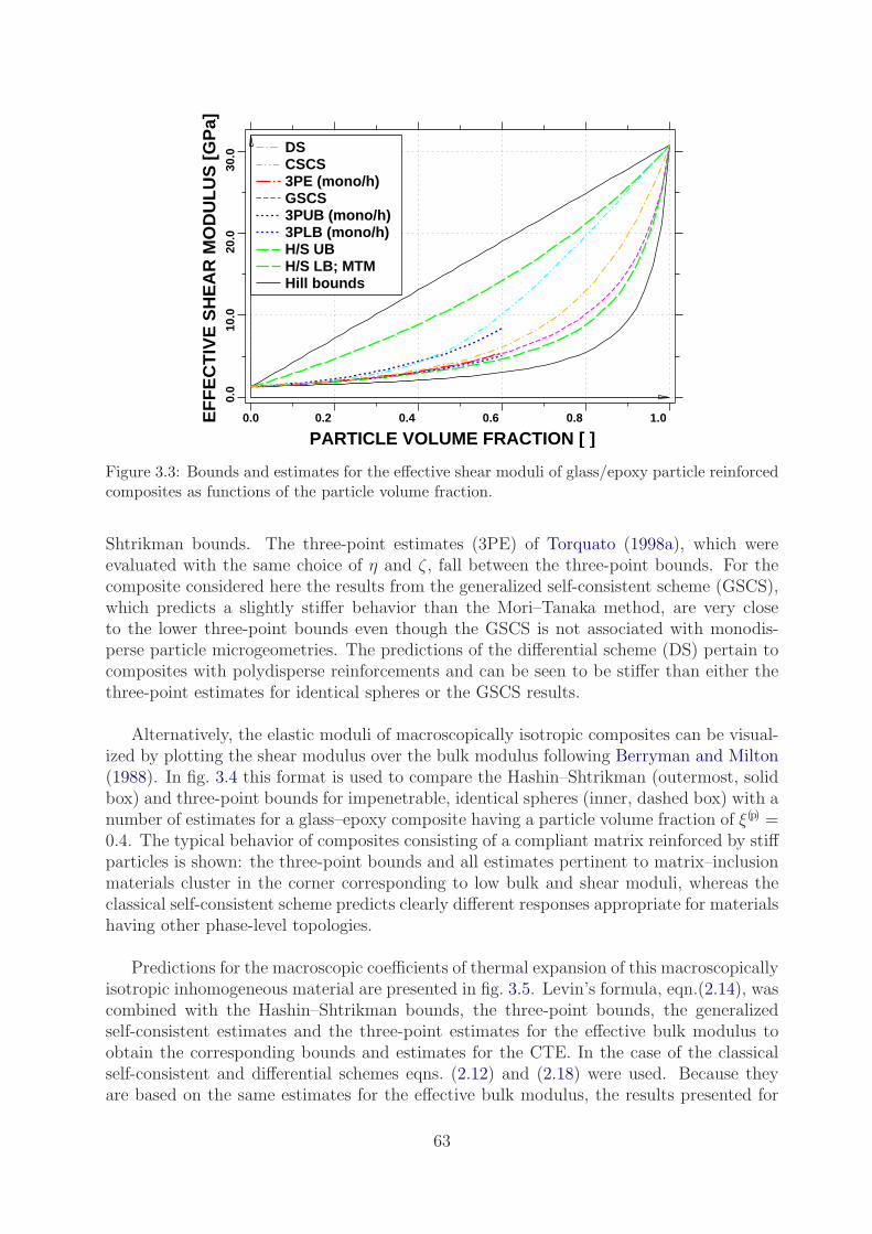
0.0

10.0

20.0

30.0

EF

FE

CT

IVE

SH

EA

R M

OD

UL

US

[G

Pa]

0.0 0.2 0.4 0.6 0.8 1.0

PARTICLE VOLUME FRACTION [ ]

Hill boundsH/S LB; MTMH/S UB3PLB (mono/h)3PUB (mono/h)GSCS3PE (mono/h)CSCSDS

Figure 3.3: Bounds and estimates for the effective shear moduli of glass/epoxy particle reinforcedcomposites as functions of the particle volume fraction.

Shtrikman bounds. The three-point estimates (3PE) of Torquato (1998a), which wereevaluated with the same choice of η and ζ, fall between the three-point bounds. For thecomposite considered here the results from the generalized self-consistent scheme (GSCS),which predicts a slightly stiffer behavior than the Mori–Tanaka method, are very closeto the lower three-point bounds even though the GSCS is not associated with monodis-perse particle microgeometries. The predictions of the differential scheme (DS) pertain tocomposites with polydisperse reinforcements and can be seen to be stiffer than either thethree-point estimates for identical spheres or the GSCS results.

Alternatively, the elastic moduli of macroscopically isotropic composites can be visual-ized by plotting the shear modulus over the bulk modulus following Berryman and Milton(1988). In fig. 3.4 this format is used to compare the Hashin–Shtrikman (outermost, solidbox) and three-point bounds for impenetrable, identical spheres (inner, dashed box) with anumber of estimates for a glass–epoxy composite having a particle volume fraction of ξ(p) =0.4. The typical behavior of composites consisting of a compliant matrix reinforced by stiffparticles is shown: the three-point bounds and all estimates pertinent to matrix–inclusionmaterials cluster in the corner corresponding to low bulk and shear moduli, whereas theclassical self-consistent scheme predicts clearly different responses appropriate for materialshaving other phase-level topologies.

Predictions for the macroscopic coefficients of thermal expansion of this macroscopicallyisotropic inhomogeneous material are presented in fig. 3.5. Levin’s formula, eqn.(2.14), wascombined with the Hashin–Shtrikman bounds, the three-point bounds, the generalizedself-consistent estimates and the three-point estimates for the effective bulk modulus toobtain the corresponding bounds and estimates for the CTE. In the case of the classicalself-consistent and differential schemes eqns. (2.12) and (2.18) were used. Because theyare based on the same estimates for the effective bulk modulus, the results presented for

63

3

4

5

6

7

8

9

7 8 9 10 11 12 13 14

EFF

EC

TIV

E S

HE

AR

MO

DU

LU

S [G

Pa]

EFFECTIVE BULK MODULUS [GPa]

HSB3PB

MTMGSCS

3PEDS

CSCS

Figure 3.4: Bounds and estimates for the effective bulk and shear moduli of a glass/epoxy particlereinforced composite of particle volume fraction ξ(p) = 0.4.

the GSCS and the Mori–Tanaka-scheme coincide with the upper Levin/Hashin–Shtrikmanbounds.

0.0

20.0

40.0

EF

FE

CT

IVE

CT

E [

1/K

x 1

0 ]-6

0.0 0.2 0.4 0.6 0.8 1.0

PARTICLE VOLUME FRACTION [ ]

H/S LBH/S UB; MTM3PLB (mono/h)3PUB (mono/h)GSCS3PE (mono/h)CSCSDS

Figure 3.5: Bounds and estimates for the effective CTEs of glass/epoxy particle reinforced com-posites as functions of the particle volume fraction.

Applying the constituent data given in table table 3.1 to an epoxy matrix reinforcedby continuous aligned glass fibers gives rise to transversally isotropic macroscopic behav-ior. Pertinent results are presented in figs. 3.6 to 3.10 for the overall transverse Young’s

64

0.0

40.0

80.0

EF

FE

CT

IVE

YO

UN

Gs

MO

DU

LU

S [

GP

a]

0.0 0.2 0.4 0.6 0.8 1.0

FIBER VOLUME FRACTION [ ]

Hill boundsH/S LB; MTMH/S UB3PB LB (mono/h)3PB LB (mono/h)GSCS3PE (mono/h)CSCSDS

Figure 3.6: Bounds and estimates for the effective transverse Young’s moduli of glass/epoxy fiberreinforced composites as functions of the fiber volume fraction.

moduli48, the overall axial and transverse shear moduli, as well as the overall axial andtransverse coefficients of thermal expansion. The results for the three-point bounds shownare based on the formalisms of Silnutzer (1972) and Milton (1981), correspond to a mi-crogeometry of aligned impenetrable circular cylindrical fibers of equal diameter, and use

0.0

10.0

20.0

30.0

EF

FE

CT

IVE

SH

EA

R M

OD

UL

US

[G

Pa]

0.0 0.2 0.4 0.6 0.8 1.0

FIBER VOLUME FRACTION [ ]

Hill boundsH/S LB; MTMH/S UB3PLB (mono/h)3PUB (mono/h)GSCS3PE (mono/h)CSCSDS

Figure 3.7: Bounds and estimates for the effective axial shear moduli of glass/epoxy fiber rein-forced composites as functions of the fiber volume fraction.

48The estimates and bounds for the axial Young’s moduli are indistinguishable from each other (and

from the rule-of-mixture result, E∗

A = ξE(i)A +(1− ξ)E(m), as well as the Hill upper bound given in fig. 3.6)

for the scaling used in fig. 3.6 and are, accordingly, not shown.

65

0.0

10.0

20.0

30.0

EF

FE

CT

IVE

SH

EA

R M

OD

UL

US

[G

Pa]

0.0 0.2 0.4 0.6 0.8 1.0

FIBER VOLUME FRACTION [ ]

Hill boundsH/S LB; MTMH/S UB3PLB (mono/h)3PUB (mono/h)GSCS3PE (mono/h)CSCSDS

Figure 3.8: Bounds and estimates for the effective transverse shear moduli of glass/epoxy fiberreinforced composites as functions of the fiber volume fraction.

statistical parameters evaluated by Torquato and Lado (1992) for fiber volume fractionsξ / 0.7. The coefficients of thermal expansion were evaluated on the basis of the relationsof Rosen and Hashin (1970).

Generally, a qualitatively similar behavior to the particle reinforced case can be ob-served. It is noteworthy that the overall transverse CTEs in fig. 3.10 at low fiber volume

0.0

20.0

40.0

EF

FE

CT

IVE

CT

E [

1/K

x 1

0 ]-6

0.0 0.2 0.4 0.6 0.8 1.0

FIBER VOLUME FRACTION [ ]

H/S LB; MTM,GSCSH/S UB3PLB (mono/h)3PUB (mono/h)3PE (mono/h)CSCSDS

Figure 3.9: Estimates and bounds for the effective axial CTEs of glass/epoxy fiber reinforcedcomposites as functions of the fiber volume fraction.

66

fractions exceeds the CTEs of both constituents. Such behavior is typical for continuouslyreinforced composites and is caused by the marked axial constraint enforced by the fibers.As expected for continuously reinforced materials, there is little variation between the pre-dictions of the different models for the axial thermal expansion behavior, fig. 3.9. TheMori–Tanaka estimates correspond to the upper bound for the transverse CTE in analogyto the macroscopically homogeneous case. For the axial CTE, however, the Mori–Tanakaresults agree with the lower bound, which is a consequence of the axial constraint intro-duced by the fibers.

0.0

20.0

40.0

EF

FE

CT

IVE

CT

E [

1/K

x 1

0 ]-6

0.0 0.2 0.4 0.6 0.8 1.0

FIBER VOLUME FRACTION [ ]

H/S LBH/S UB; MTM,GSCS3PLB (mono/h)3PUB (mono/h)3PE (mono/h)CSCSDS

Figure 3.10: Estimates and bounds for the effective transverse CTEs of glass/epoxy fiber rein-forced composites as functions of the fiber volume fraction.

In figs. 3.2 to 3.8 the classical self-consistent scheme is not in good agreement withthe three-point bounds shown, because the latter explicitly correspond to matrix–inclusiontopologies. Considerably better agreement with the CSCS can be obtained by using three-point parameters of the overlapping sphere or cylinder type (which can also describe caseswhere both phases percolate, but are not as symmetrical with respect to the constituents asthe CSCS). From a practical point of view it is worth noting that despite their sophistica-tion higher order estimates (and improved bounds) may give overly optimistic predictionsfor the overall moduli because they describe ideal composites, whereas in actual “two-phase” materials it is practically impossible to avoid flaws such as porosity.

Before closing this chapter it is worth mentioning that more complex responses maybe obtained when at least one of the constituents is transversely isotropic and one of theelastic or conductivity contrasts exceeds unity whereas the other is smaller (such situationscan occur, e.g., in metals reinforced by carbon fibers). Also, the differences between thepredictions of different mean-field models typically tend to be more pronounced when thesealgorithms are used to describe nonlinear responses, e.g., elastoplastic behavior. Further-more, the angular dependences of stiffnesses and CTEs in fiber reinforced materials can bequite rich, compare, e.g., Pettermann et al. (1997).

67

3.6 Comparisons of Mean-Field and Bounding Pre-

dictions for Effective Conductivities

Predictions for the effective conductivities of composites as functions of the phase volumefractions are qualitatively similar to the corresponding data for the elastic moduli, as can beseen in figs. 3.11 and 3.12, which pertain to a polyetherimide matrix reinforced by alignedshort graphite fibers of aspect ratio a = 10. The plots use material parameters given byHarte and Mc Namara (2006), which are listed in table 3.2. The fibers show transversallyisotropic conductivity, the axial conductivity contrast taking a value of approximately 37,whereas the transverse conductivity contrast is an order of magnitude smaller.

Table 3.2: Constituent material parameters of polyetherimide matrix and the T-300 graphitefibers used in generating figs. 3.11 to 3.12.

kA[Wm−1K−1] kT[Wm−1K−1]matrix 0.22 0.22reinforcements 8.40 0.84

Because for the composite described by figs. 3.11 and 3.12 the matrix conductivity issmaller than either the axial or the transverse fiber conductivities, the Mori–Tanaka es-timates for the effective conductivity coincide with the lower Hashin–Shtrikman bounds.Even though the selected fiber aspect ratio is rather moderate, the macroscopic conduction

0.0

4.0

8.0

EF

FE

CT

IVE

CO

ND

UC

TIV

ITY

[W

/mK

]

0.0 0.2 0.4 0.6 0.8 1.0

FIBER VOLUME FRACTION [ ]

Wiener boundsH/S LB; MTMH/S UBCSCSDS

Figure 3.11: Bounds and estimates for the effective axial conductivity of composites consisting ofaligned short graphite fibers (a = 10) in a polyetherimide matrix as functions of the fiber volumefraction.

68

0.0

0.4

0.8

EF

FE

CT

IVE

CO

ND

UC

TIV

ITY

[W

/mK

]

0.0 0.2 0.4 0.6 0.8 1.0

FIBER VOLUME FRACTION [ ]

Wiener boundsH/S LB; MTMH/S UBCSCSDS

Figure 3.12: Bounds and estimates for the effective transverse conductivity of composites con-sisting of aligned short graphite fibers (a = 10) in a polyetherimide matrix as functions of thefiber volume fraction.

behavior approaches that of a continuously reinforced composite, with the upper Wienerand Hashin–Shtrikman bounds being nearly identical. As in the elastic case the classicalself-consistent scheme, which does not describe matrix–inclusion topologies for all volumefractions, is close to one Hashin–Shtrikman bound at low fiber volume fractions and closeto the other at high ones. The predictions of the differential scheme differ rather stronglyfrom the lower Hashin–Shtrikman bounds, a behavior that tends to be especially marked inmaterials with elevated conductivity contrasts (which may reach very high values, indeed,in the case of electrical conduction).

69

Chapter 4

General Remarks on ModelingApproaches Based on DiscreteMicrostructures

In the following, micromechanical approaches based on discrete microstructures are un-derstood to encompass the periodic homogenization, embedding and windowing methodsdiscussed in chapters 5 to 7 and sketched in fig. 1.1. Broadly speaking, these “full fieldmodels” trade off potential restrictions to the generality of the phase arrangements againstthe capability of using fine-grained geometrical descriptions and of resolving details of thestress and strain fields at the length scale of the inhomogeneities49. The most importantapplications of such methods are homogenizing the behavior of inhomogeneous materialsand evaluating the microscopic stress and strain fields in relevant microgeometries at highresolution. The latter information, on the one hand, is important when the local fieldsfluctuate strongly and, consequently, much information is lost by volume averaging. Onthe other hand, it is important for understanding the damage and failure behavior of in-homogeneous materials, which in many cases depends on details of their microgeometry.

The most common work flow in models involving discrete microstructures consists offirst obtaining appropriate phase arrangements, see section 4.1, discretizing the resultingvolume elements and preparing them for application of a numerical engineering method, seesections 4.2 and 4.3, solving for the microfields, and, finally, postprocessing, see section 4.4.

4.1 Microgeometries and Volume Elements

The heterogeneous volume elements (“microgeometries”) used in full field models rangefrom highly idealized periodic geometries (“simple periodic arrays”), such as cubic arraysof spheres in a matrix, to large phase arrangements that aim at closely approximatingthe geometrical complexity and/or arrangement statistics of actual inhomogeneous mate-rials (“microstructural volume elements”). There are two main strategies for generatingheterogeneous volume elements for modeling, viz., using synthetic microstructures, usu-

49Such methods by construction aim at resolving inter-particle and intra-particle interactions at themaximum level attainable within continuum mechanics.

70

ally obtained from computer-based simulations, or employing phase arrangements that aredirectly based on microgeometries obtained by experimental methods. The following con-siderations concentrate on microgeometries with matrix–inclusion topology.

Synthetic Phase Arrangements

Synthetically generated volume elements that go beyond simple periodic arrays may beclassified into two groups, the first of which makes use of volume elements that containgeneric arrangements of a number of randomly positioned and, where appropriate, ran-domly oriented, sized, or shaped reinforcements. The second group aims at constructingphase arrangements that have phase distribution statistics identical to those of the targetmaterial. A further possible approach to synthesizing realistic volume elements by com-puter algorithms, which consists of modeling relevant production processes, has seen littleuse to date for composites due to the complexity of the task. Synthetic volume elementshave found wide use for studying composites with matrix–inclusion and interpenetratingphase arrangements, polycrystals as well as cellular materials. For a recent review on gen-erating three-dimensional inhomogeneous volume elements see Bargmann et al. (2018).

Synthesizing generic “multi-inhomogeneity” model geometries with random arrange-ments of reinforcements in many cases has involved random sequential addition methods50.The reinforcement volume fractions that can be reached by RSA methods tend to be mod-erate due to jamming (“geometrical frustration”), however, their representativeness foractual phase arrangements generated by mixing processes is open to question (Stroevenet al., 2004), and they may give rise to biased phase arrangements (Pontefisso et al., 2016).Major improvements can be obtained by using RSA geometries, or, in the case of very hightarget inhomogeneity volume fractions, packings obtained by methods such as collectiverearrangement models, see, e.g., Maggi et al. (2008), as starting configurations for ran-dom perturbation, “hard core shaking” or migration models, compare, e.g., Buryachenkoet al. (2003) or Schneider (2017). Such algorithms apply small random displacements toeach inhomogeneity to obtain improved and, if the size of the volume element is reducedin the process, more tightly packed arrangements of reinforcements. Alternatively, RSAmethods may be combined with stirring models (Zangenberg and Brøndsted, 2013) orwith optimization procedures (Pathan et al., 2017) to obtain higher inhomogeneity volumefractions. RSA based approches have been used to generate (approximately) statisticallyhomogeneous distributions of particulate or fibrous reinforcements, see, e.g., Gusev (1997),Bohm and Han (2001), Lusti et al. (2002), Duschlbauer et al. (2006) or Rasool and Bohm(2012), as well as idealized clustered microgeometries (Segurado et al., 2003), and they can

50In random sequential addition (RSA) algorithms (also known as random sequential insertion or randomsequential adsorption models, and sometimes referred to as “static simulations”), positions and, where ap-plicable, orientations for new reinforcements are created by random processes, a candidate inhomogeneitybeing accepted if it does not “collide” with any of the existing ones and rejected otherwise. In contrast torandom packing, in generating microgeometrical models a “collision” often involves the violation of someminimum distance rather than actual touching of (or overlapping with) neighboring inhomogeneities.Whereas collision checking is straightforward with circular or spherical inhomogeneities, algorithms suchas the separating axis method (Schneider and Eberly, 2003) may be required for polyhedral shapes.If periodic phase arrangements are generated, up to 8 periodic copies must be maintained for any inho-mogeneity that is intersected by one or more faces of the volume element.

71

be adapted for obtaining volume elements that follow prescribed fiber orientation distri-butions, see, e.g., Schneider (2017).

Matrix–inclusion configurations of elevated inhomogeneity volume fraction can be ob-tained by “random particle dropping” (Chiaia et al., 1997) or gravitational methods (Khale-vitsky and Konovalov, 2019), discrete-element-based models (Ismail et al., 2016), particleexpansion methods (Zhang et al., 2019), or molecular-dynamics-like algorithms (Lubachevskyet al., 1991), which are also known as collective rearrangement models, see, e.g., Ghosseinand Levesque (2013). Furthermore, arrangements of particles in composites may be gen-erated via hydrodynamic interactions in a pseudo-fluid (Elliott and Windle, 2000). For adiscussion of methods for generating geometrically complex volume elements containing fi-brous inhomogeneities that are compliant in bending, see, e.g., Altendorf and Jeulin (2011).

Additional approaches to generating multi-inhomogeneity synthetic volume elementswith matrix–inclusion topology have been based on “eroding” (or shrinking) the individ-ual cells of suitable Voronoi tesselations (Fritzen and Bohlke, 2011) of the whole volumeor on first filling the unit cell with tetrahedra which are then assigned to the requiredphases by a suitable algorithm (Galli et al., 2008), randomness being introduced via theunderlying tesselation in both cases. Both methods result in arrangements of randomlypositioned and oriented inhomogeneities of irregular polygonal or polyhedral shape, thefirst mentioned one being applicable to a wide range of inhomogeneity volume fractions.

The most important alternative strategy for generating volume elements by simula-tion aims at obtaining “statistically reconstructed” phase arrangements, which are notidentical to any given sample, but rather are statistically equivalent to the material tobe modeled. Statistical reconstruction typically gives rise to optimization problems inwhich some starting configuration (e.g., a periodic phase arrangement of appropriate vol-ume fraction) is modified such that suitable statistical and/or stereological descriptorsof the phase distributions approach the chosen target descriptor(s) as closely as possi-ble. Procedures for reconstructing matrix–inclusion and more general microgeometrieshave been reported that employ simulated annealing procedures (Rintoul and Torquato,1997; Torquato, 1998b; Bochenek and Pyrz, 2004), genetic algorithms (Zeman and Sejnoha,2001), and other minimization methods (Roberts and Garboczi, 1999). For in-depth dis-cussions of the underlying issues, such as statistical descriptors for the phase arrangementsof inhomogeneous materials, see, e.g., Torquato (2002) or Zeman (2003); questions of theuniqueness of reconstructed two-phase microgeometries were discussed by Jiao et al. (2007).Alternative approaches to statistical reconstruction were reported, e.g., by Vaughan andMcCarthy (2010) or de Francqueville et al. (2019). Studies on statistical reconstructionhave been based on a number of statistical descriptors of phase arrangements, among themn-point, nearest neighbor and radial distribution functions as well as correlation functions,i.e., they follow the concept of geometrical RVEs discussed in section 1.3. Microstructuresgenerated by statistical reconstruction are especially attractive because the phase arrange-ments in at least some actual composites were found to be not completely spatially random(Trias, 2005). For volume elements that contain considerable numbers of inhomogeneitiesor other microstructural features, statistically reconstructed phase arrangements are morespecific to a given target material than are generic random microgeometries. Because atpresent computational requirements limit the sizes of volume elements that can be handled

72

routinely by numerical engineering methods, this advantage has been of limited practicalimpact in the context of continuum micromechanics. This issue can be addressed by theconcept of “statistically similar volume elements”, in which volume elements of smallersize than RVEs are optimized to approach statistical descriptors of the target material asclosely as possible, see, e.g., Balzani et al. (2010) and Scheunemann et al. (2015).

Synthetically generated matrix–inhomogeneity microgeometries have tended to employidealized reinforcement shapes, equiaxed particles embedded in a matrix, for example,being often represented by spheres, and fibers by cylinders or prolate spheroids51 of appro-priate aspect ratio. However, recent work has also targeted polyhedral inhomogeneities,see, e.g., Nogales and Bohm (2008), Rasool and Bohm (2012), Zhang et al. (2014), Shenget al. (2016) or Bohm and Rasool (2016).

Real Structure Phase Arrangements

Instead of generating phase arrangements by computer algorithms, volume elements maybe chosen to follow as closely as possible the actual microgeometry in some appropriatesubvolume of the material to be modeled, obtained from metallographic sections (Fisch-meister and Karlsson, 1977), serial sections (Terada and Kikuchi, 1996; Li et al., 1999),tomographic data (Hollister et al., 1994; Kenesei et al., 2004; Chawla and Chawla, 2006;Buffiere et al., 2008), etc. The resulting volume elements are often called “real microstruc-ture” models.

The generation of real structure models from pixel (digital images) or voxel (tomo-graphic) data describing the geometries of inhomogeneous materials has been the focus ofconsiderable research efforts. Such work involves the steps of selecting from experimentaldata sets appropriate volume elements for analysis (“registration”) and of identifying theregions occupied by the different constituents by thresholding of the grey values of the pix-els or voxels (“segmentation”). At this stage pixel or voxel models (compare section 4.3)can be generated directly from the segmented data set or contouring procedures may beused for obtaining “smooth” phase domains, the latter operation typically being more man-power intensive52. Alternatively, irregular particle shapes in real structure arrangementshave been approximated by ellipsoids of appropriate size, shape and orientation, compareLi et al. (1999). Computed tomography has proven especially useful for determining themicrogeometries of inhomogeneous materials with constituents that differ considerably inX-ray absorption, e.g., porous and cellular materials.

Real microstructure models provide accurate descriptions of actual phase arrangements,which, however, may depend to a considerable extent on details of the underlying experi-ments, e.g., the resolution of the digital images, as well as of the registration, segmentation

51For uniform boundary conditions it can be shown that the overall elastic behavior of matrix–inclusiontype composites can be bounded by approximating the actual shape of particles by inner and outer en-velopes of “smooth” shape, e.g., inscribed and circumscribed ellipsoids. This is known as the Hill modi-fication theorem (Hill’s comparison theorem, auxiliary theorem or strengthening theorem), compare Hill(1963) and Huet et al. (1990). Approximations of actual inhomogeneity shapes by ellipsoids typically workconsiderably better for convex than for non-convex particle shapes (Kachanov and Sevostianov, 2005).

52For a review of work directed at automatically generating high quality structured meshes from voxeldata sets, see, e.g., Young et al. (2008).

73

and, where applicable, smoothing procedures. In general, the resulting volume elementsobviously are non-periodic, which restricts their use with the periodic homogenization tech-niques discussed in chapter 5, but makes them well suited to windowing and embeddingapproaches, compare chapters 6 and 7. For a discussion of three-dimensional sampling ofgeneral microstructures and the categorization of a variety of types of resulting volumeelements see Echlin et al. (2014).

Sizes of Volume Elements

When small volume elements are used in full field simulations, the predicted macroscopicresponses tend to show a marked dependence on the size of the volume elements, see, e.g.,Iorga et al. (2008). This immediately raises the question of the size of volume elementrequired for adequately capturing the macroscopic physical behavior of the material to bestudied53. On the one hand, the requirement of limiting numerical cost obviously puts apremium on using the smallest viable volume element but, on the other hand, resolvingmicrogeometry effects militates for using microgeometries that are or approximate repre-sentative volume elements (RVEs, compare section 1.3). These conflicting demands ledto the concepts of “minimum RVEs” by Ren and Zheng (2004), of “statistical RVEs” byTrias et al. (2006), of P-SERVEs by Swaminathan et al. (2006) and of statistical volumeelements by Ostoja-Starzewski (2006).

When the philosophy of geometrical RVEs is followed, estimates for suitable sizes ofvolume element can be obtained on the basis of descriptors of the microgeometry alone,the physical property to be modeled playing no role. In such a context the adequacy ofthe size of a volume element may be assessed, e.g., on the basis of experimentally obtainedcorrelation lengths (Bulsara et al., 1999) or covariances (Jeulin, 2001) of the phase ar-rangement or by posing requirements such as having at least two statistically independentinhomogeneities in the volume element (Zeman and Sejnoha, 2001). Such approaches canbe extended to anisotropic microgeometries (Wang et al., 2019) and they have proven suc-cessful for micromechanical models of the elastic behavior of inhomogeneous materials.

The concept of physical RVEs as stated in section 1.3, in contrast, implies that thesuitability of a given size of volume element for micromechanical modeling depends onthe physical property to be studied. Assessing the representativeness of a volume elementin this sense can, in principle, be carried out by windowing analysis, compare chapter 6,with identical predictions of the macroscopic behavior under macroscopically homogeneousstress and strain boundary conditions, respectively, being indicative of physical RVEs inthe strict sense. In practice, this criterion has proved to be difficult to fulfill in a rigorousway, and, consequently, the suitability of volume elements for a given task is typicallyassessed by specifying appropriate thresholds or by checking some necessary criteria forrepresentativeness. The most important approach of this type is based on studying theconvergence of estimates for the macroscopic behavior with growing size of the volume el-ements, compare, e.g., Savvas et al. (2016). Furthermore, the compliance of the predictedeffective responses with tight bounds (e.g., three-point bounds in the case of randomly

53Traditionally, RVEs have been defined in terms of macroscopic responses. Assessing higher statis-tical moments of phase-level microstresses in addition to the first one (which underlies modulus-basedconsiderations) appears feasible but may lead to more stringent requirements on RVEs.

74

positioned spheres of moderate phase contrast) and the attaining of appropriate macro-scopic material symmetry may be checked for. For comparisons of different geometry andmicrofield based criteria for choosing the size of model geometries see, e.g., Trias et al.(2006) and Moussaddy et al. (2013). It must be kept in mind, though, that fulfilling thelatter criteria — while going a considerable way towards ensuring useful modeling results— is not sufficient for establishing proper RVEs.

Assessments based solely on the geometry or on the overall elastic behavior predictthat relatively small volume elements can give fairly accurate results. Zeman (2003) re-ported that the transverse elastic behavior of composites reinforced by continuous fiberscan be satisfactorily described by unit cells containing reconstructed arrangements of 10to 20 fibers. “Pragmatic” definitions, in which a given volume element must fulfill somegiven criterion to a specified accuracy to be accepted as a physical RVE, have been usedto a considerable extent. Using a nonlocal Hashin–Shtrikman model Drugan and Willis(1996) found that, for statistically isotropic composites consisting of a matrix reinforcedby spherical particles, volume elements with sizes of some two and five particle diametersare sufficient for obtaining errors of less than 5% and less than 1%, respectively, in termsof the macroscopic elastic stiffness. Interestingly, these sizes of volume elements come outas being independent of the particle volume fraction54, a prediction that is not shared byalternative models for assessing RVE sizes (Pensee and He, 2007; Xu and Chen, 2009).Considerably larger volume elements are required for obtaining a given level of accuracyfor aligned ellipsoidal inhomogeneities, where the RVE size depends on the reinforcementvolume fraction (Monetto and Drugan, 2009), and different estimates for the RVE sizeresult when modeling elastic and thermal conduction behavior (Kanit et al., 2003).

For cases involving inelastic constituent behavior, a number of numerical studies (Zohdi,1999; Jiang et al., 2001; Bohm and Han, 2001) have indicated that larger volume elementstend to be required for satisfactorily approximating the overall symmetries and for obtain-ing good agreement between the responses of different phase arrangements designed to bestatistically equivalent. More recent studies (Cugnoni and Galli, 2010; Galli et al., 2012;Zhang et al., 2014) have confirmed the need for relatively large volume elements in orderto approach representativeness in elastoplastic composites, especially at elevated strains.They report a clear dependence of the RVE size on the inhomogeneity volume fractionand on the macroscopic strain for particle reinforced ductile matrix composites. The mainreason for this behavior lies in the marked inhomogeneity of the microscopic strain fieldsthat is typically present in nonlinear composites. For example, there tend to be contiguouszones of concentrated plastic strains, evolve to become considerably larger than individualreinforcements, thus effectively introducing a new length scale into the problem55. In the

54For a given level of uncertainty, this corresponds to the number of identical inhomogeneities withinthe volume element scaling with their volume fraction, ξ.

55In the hardening regime, phase arrangements with high reinforcement volume fractions may give rise tosmaller RVEs than do volume elements with moderate ones, the inhomogeneities impeding the formationof zones of concentrating plastic strain (Cugnoni and Galli, 2010). For elastoplastic matrices, weaker strainhardening typically produces more inhomogeneous microstrains, which leads to a requirement for volumeelements that contain a higher number of inhomogeneities. Extremely large volumes were reported tobe necessary when one of the phases shows softening, e.g., due to damage (Zohdi and Wriggers, 2001;Swaminathan and Ghosh, 2006; Gitman, 2006). For elastic polycrystals, the anisotropy and shape of thegrains were also reported to influence the required size of volume elements (Ren and Zheng, 2004).

75

case of path dependent material behaviors assessments of the suitability of a given volumeelement, strictly speaking, pertain only to the load paths actually considered. Eliminatingthe dependence of the homogenized response on the size of the volume element can beargued, in fact, to become impossible in the presence of strain localization (Gitman et al.,2007), the statistical homogeneity of the whole sample or component being lost. Largevolume elements are also required for materials the behavior of which depends stronglyon “rare features” of the microgeometry, see, e.g., Przybyla and McDowell (2010), and forconfigurations that contain markedly non-equiaxed phase regions, e.g., randomly orientedfibers of elevated aspect ratio. Comparisons between equivalent volume element sizes forvarious macroscopic behaviors of two-dimensional inhomogeneous materials were reportedby Ostoja-Starzewski et al. (2007).

Modeling work in most cases has been based on volume elements that are known tobe of insufficient size to be proper RVEs, the main reasons for using them being limits inthe size of models that can be handled and difficulties in providing suitable RVEs for ac-tual materials. Such “sub-RVE” volume elements, which may be periodic or non-periodic,are referred to as statistical volume elements (SVEs, Ostoja-Starzewski (2006)), testingvolume elements (TVEs, Diebels et al. (2005)) or windows, compare chapter 6 — simplycalling them RVEs is not good practice. When a number of SVEs of comparable volumeand pertaining to a given inhomogeneous material are available, they may be viewed asbeing different realizations of the phase arrangement statistics describing that material.In such cases ensemble averaging over the results obtained from sets of volume elementscan be used to obtain improved estimates for the effective material properties, compare,e.g., Kanit et al. (2003) and Stroeven et al. (2004). The number of different volume ele-ments required for a given level of accuracy of the ensemble averages decreases as their sizeincreases (Khisaeva and Ostoja-Starzewski, 2006). As to using a lower number of largervs. a higher number of smaller volume elements, Harper et al. (2012b) reported that theformer option is more efficient56 Furthermore, for macroscopically isotropic materials theanisotropic contributions to the ensemble averaged results was reported to be markedlyreduced compared to the predictions of the individual SVEs (El Houdaigui et al., 2007). Itwas, however, reported by Galli et al. (2012) that ensemble averaging over non-periodic sta-tistical volume elements in the elastoplastic range may be compromised by boundary layers.

For linear properties Kanit et al. (2003) proposed confidence intervals for assessingthe quality of the ensemble averaged results obtained from sets of SVEs. In this contextan error measure can be defined in terms of the standard deviation S(Y ) of some givenmodulus or tensor element, Y , as

err(Y ) =1.96S(Y )√

nSVE

, (4.1)

where nSVE is the number of statistically equivalent SVEs used in ensemble averaging. Arelated approach for nonlinear behavior was proposed by Pelissou et al. (2009). A furtherrefinement consists in weighting the contributions of the SVEs according to statistical pa-rameters (Qidwai et al., 2012).

56This result is subject to the caveat that in practice volume elements exceeding a certain size, determinedby limitations of the available hardware and the spatial resolution of the discretization used, cannot behandled with comparable efficiency as smaller ones.

76

The size of the volume element(s) used in modeling affects not only the macroscopicresponses, but also the predicted microfields. Accordingly, some authors have explored thequestion of what size of volume element is required for studying the local fields at somespecific location. This may be done by studying series of volume elements of different sizethat pertain to a given microstructure, see, e.g., Ozturk et al. (2016).

As to the dimensionality of volume elements, for composites reinforced by aligned, con-tinuous fibers two-dimensional VEs can be used for studying most (but not all) load casesin linear and nonlinear regimes, compare section 5.4. For composites containing particles,platelets and/or short fibers, however, three-dimensional volume elements are in generalnecessary, see, e.g., Iung and Grange (1995), Bohm and Han (2001) and Weidt and Figiel(2014) as well as sections 5.5 and 5.6.

4.2 Boundary Conditions

As the size of volume elements describing inhomogeneous materials is increased, the re-sulting predictions of the apparent overall behavior improve until representativeness isachieved, when further increases in model size do not lead to further changes in the resultsand the effective behavior is obtained. The rate of convergence towards proper effectivebehavior depends on the boundary conditions applied to the volume element.

Fulfilling the surface integral version of the Hill–Mandel condition, eqn. (1.7), whichcan be written in the form57

∫

Γ

[t(x)− 〈σ〉 ∗ nΓ(x)

]T[u(x)− 〈ε〉 ∗ x

]dΓ = 0 , (4.2)

see Hill (1967) and Hazanov (1998), for inhomogeneous volume elements of finite size, canbe achieved by four types of boundary conditions, three of which are based on uniformB.C.s (Hazanov and Amieur, 1995; Ostoja-Starzewski, 2006).

First, the traction term in eqn. (4.2) can be made to vanish over the whole boundary byspecifying appropriate Neumann (“natural”) boundary conditions for the tractions t(x).These are obtained by prescribing a macroscopically homogeneous stress tensor σa on allfaces of the volume element,

t(x) = σa ∗ nΓ(x) ∀x ∈ Γ , (4.3)

leading to statically uniform boundary conditions (SUBC, or uniform Neumann BC, UNBC).

Second, the right hand term in eqn. (4.2) can be enforced to be zero by imposing agiven macroscopically homogeneous strain tensor εa on all boundary surfaces,

u(x) = εa ∗ x ∀x ∈ Γ , (4.4)

57Equation (4.2) essentially states that energy equivalence is achieved when local fluctuations do notcontribute to the elastic strain energy density.

77

resulting in kinematically uniform boundary conditions (KUBC, uniform Dirichlet BC,UDBC, or linear displacement BC, LDBC), which, in FE parlance, are a type of essentialBC. Because eqns. (4.3) and (4.4) impose homogeneous stress or strain fields on the bound-ary of the volume element, they are known as macrohomogeneous boundary conditions.Some authors also refer to them as Hashin boundary conditions.

Third, mixed uniform boundary conditions (MUBC) may be specified, in which thescalar product under the integral is made to vanish separately for each face Γk that is partof the surface of the volume element,

[t(x)− 〈σ〉 ∗ nΓ(x)]T[

u(x)− 〈ε〉 ∗ x]

dΓ = 0 ∀x ∈ Γk . (4.5)

This involves appropriate combinations of traction and strain components that are uni-form over a given face of the volume element rather than specifying a macroscopicallyhomogeneous field. Mixed uniform boundary conditions that fulfill eqns. (4.2) and (4.5)must be orthogonal in their fluctuating contributions (Hazanov and Amieur, 1995). Thesymmetry boundary conditions discussed in section 5.2 are a type of MUBC and specificsets of MUBC useful for window-type microgeometries are presented in chapter 6.

Finally, the displacement and traction fields may be decomposed into slow and fastcontributions in analogy to eqn. (1.2),

u(x) = 〈ε〉 ∗ x + u′(x) and t(x) = 〈σ〉 ∗ nΓ(x) + t′(x) . (4.6)

Inserting these expressions into the Hill–Mandel criterion, eqn. (4.2), directly leads to thecondition ∫

Γ

t′(x)Tu′(x) dΓ = 0 , (4.7)

which are fulfilled by periodic phase arrangements. By definition, the latter can be fullydescribed by a single periodic volume element, called a unit cell, the surface of whichmust consist of pairs of parallel surface elements, compare section 5.2. For homologouspoints on such pairs of faces the stress and strain tensors must be identical, which impliesthat the displacement fluctuation vectors u′(x) at the two faces are identical, too, whereasthe traction fluctuation vectors t′(x) have equal absolute values but opposite orientations,compare fig. 4.1. As a consequence, contributions to eqn. (4.7) from each pair of homologousfaces cancel out and the Hill condition is fulfilled for the periodic unit cell itself and forlarger periodic assemblages of unit cells. A more detailed discussion of periodic unit cellsand the associated periodicity B.C. is given in section 5.2. Incidentally, if the shape ofa volume element is such that for each surface point there exists an “antipodic” pointhaving the opposite normal vector (as is the case, e.g., for spheres), eqn. (4.7) can beformally enforced in a point-wise way even for non-periodic volume elements (Gluge et al.,2012), giving rise to so-called “antipodic periodicity” boundary conditions. For a furtherdiscussion of microscopic boundary conditions see, e.g., Nguyen et al. (2017).

Macrohomogeneous boundary conditions following eqns. (4.3) and (4.4) can be shown togive rise to lower and upper estimates, respectively, for the overall elastic tensor of a givenmesoscopic volume element (Nemat-Nasser and Hori, 1993). Results obtained with mixeduniform and periodicity boundary conditions must lie between the corresponding lower

78

N

S

W E nEnW

Figure 4.1: Sketch of antiperiodic traction fluctuations at faces of periodic VE under macroscopicuniaxial tensile loading.

and upper estimates (Hazanov and Huet, 1994) and show a faster convergence towards theeffective response with increasing volume element size, periodicity B.C. being best in termsof convergence. There is, however, no guarantee that periodic boundary conditions givethe best estimates among the above four types of boundary conditions (Terada et al., 2000).

KUBC-based predictions for the elastic macroscopic behavior of fiber reinforced com-posites can be improved via an approach developed by Ghosh and Kubair (2016). Itmodifies u(x) in eqn. (4.4) by an additional, position dependent displacement contributionthat is evaluated by a modified Eshelby formalism incorporating two-point statistical in-formation on the microstructure outside the volume element.

SUBC and KUBC do not pose restrictions on the phase geometry or on the shape ofvolume elements, but some MUBC are subject to certain restrictions on the latter count,compare section 5.2. Periodic homogenization obviously requires specific volume elementsdescribing periodic phase geometries (which restricts admissible shapes), to which peri-odicity boundary conditions or, in special cases, symmetry and antisymmetry boundaryconditions are applied, see chapter 5. Antipodic boundary conditions require volume ele-ments of specific shapes, but are not restricted to periodic geometries.

In addition to the above four types of boundary condition, the Hill–Mandel criterioncan also be fulfilled by configurations in which the volume element proper is surroundedby a layer of homogeneous material that is given the effective behavior of the core. Elas-tic tensors obtained by applying macrohomogeneous or periodicity boundary conditions,eqns. (4.3) to (4.7), to the outer surface of the embedding layer can be shown to fall withinthe upper and lower estimates generated by applying the macrohomogeneous B.C. directlyto the volume element, see Temizer et al. (2013). Such configurations form the basis ofself-consistent embedding schemes, compare chapter 7. Furthermore, weak formulationsof periodicity and macrohomogeneous boundary conditions have been developed, see, e.g.,Mesarovic and Padbidri (2005) or Larsson et al. (2011).

Among the above types of models and boundary conditions only fully implementedperiodicity B.C. do not lead to boundary layers in the predicted microscopic stress and

79

strain fields58, which is an advantage since boundary perturbations may lead to spuriousbehavior when nonlinear constitutive response of the constituents is considered. Periodichomogenization also is unique in that volume elements consisting of multiple copies of agiven unit cell give rise to the same prediction as the unit cell itself (provided wave phe-nomena or buckling are not involved).

4.3 Numerical Engineering Methods

The majority of continuum micromechanical studies of discrete microstructures have em-ployed standard numerical engineering methods for resolving the microfields. Work re-ported in the literature has involved Finite Difference and Finite Volume algorithms, com-pare Adams and Doner (1967), Bansal and Pindera (2006), Cavalcante et al. (2012) orChen et al. (2016), spring lattice models, compare Ostoja-Starzewski (2002), the Bound-ary Element Method (BEM), compare Achenbach and Zhu (1989), Liu et al. (2005b) orBai et al. (2015), as well as the Finite Element Method (FEM) and its derivatives such asExtended Finite Element Methods, mesh-free, particle and isogeometric methods, compareSukumar et al. (2001), Dang and Sankar (2007) and Missoum-Benziane et al. (2007), orFE-based discrete dislocation models (Cleveringa et al., 1997). In general, spring latticemodels tend to show some advantages in handling traction boundary conditions and inmodeling the progress of microcracks due to local brittle failure. Boundary element meth-ods typically are at their best in studying geometrically complex linear elastic problems.

In addition to the above methods, techniques using Fast Fourier Transforms (FFT),compare Moulinec and Suquet (1994), and Discrete Fourier Transforms (DFT), compareMuller (1996), have found considerable use in continuum micromechanics, especially inperiodic homogenization. Typically, the starting point for such iterative algorithms is aLippmann–Schwinger equation, compare eqn. (2.32). The convolution integral in this equa-tion is solved in Fourier space (where it reduces to a tensor contraction) and the strains areupdated in physical space within each iteration, transforms and back transforms betweenthe two spaces being handled by fast numerical algorithms. Such spectral methods aredirectly applicable to analyzing periodic volume elements, where they tend to be highlyefficient, compare, e.g., Michel et al. (1999) or Ghossein and Levesque (2012), for bothlinear and nonlinear phase behavior. Further developments of these approaches have al-lowed the handling of infinite phase contrasts (Brisard and Dormieux, 2010) and nonlinearproblems (Schneider, 2021). Homogenization via FFT at present is a highly active researchfield and FFT-based schemes are becoming the methods of choice for handling very large,periodic, voxel-type models. DFT methods have found use in studying the evolution ofmicrostructures (Dreyer et al., 1999).

A further approach, the Transformation Field Analysis of Dvorak (1992), allows theprediction of the nonlinear responses of inhomogeneous materials based on either mean-field descriptions (compare the remarks in section 2.5) or on full field approximations.

58Perturbations caused by the application of uniform boundary conditions to inhomogeneous surfaces orby the local incompatibility between homogenized and inhomogeneous regions depend on the local materialcontrasts and do not necessarily become smaller with increasing volume element size.

80

High computational efficiency is claimed for “classical” TFA models employing piecewiseuniform transformation fields (Dvorak et al., 1994), and the extension to FE2-type modelshas been reported (Marfia and Sacco, 2018). A development of the TFA, the NonuniformTransformation Field Analysis (Michel and Suquet, 2004), expands the inelastic strains intoa number of non-uniform, incompressible and orthogonal “plastic flow modes” to achieveefficient descriptions of the elastoplastic behavior of inhomogeneous materials.

Furthermore, integral equations describing the displacement, stress and strain fields ininhomogeneous materials may be solved by numerical integration schemes, compare, e.g.,Lee et al. (2011a) or Tashkinov (2021). For a number of additional numerical approachesthat have been mainly used for periodic homogenization see section 5.1.

Obviously, when numerical engineering methods are used in continuum micromechanics,the characteristic length of the discretization (“mesh size”) must be chosen considerablysmaller than the microscale of the considered problem in order to obtain spatially wellresolved results.

At present, the FEM is the most popular numerical scheme for evaluating full field mod-els, especially in the nonlinear range, where its flexibility and capability of supporting awide range of constitutive descriptions for the constituents and the interfaces between themare especially appreciated59. An additional asset of the FEM in the context of continuummicromechanics is its ability to handle discontinuities in the stress and strain components(which typically occur at interfaces between different constituents) in a natural way viaappropriately placed element boundaries. Furthermore, Finite Element codes are widelyavailable and many of them provide linear constraint equations for coupling multiple de-grees of freedom, which are required for periodic homogenization, compare section 5.2.

Applications of (more or less) standard Finite Element methods to micromechanicalstudies may be classed into five main groups, compare fig. 4.2, all of which involve specifictrade-offs in terms of complexity of the models, required meshing effort, computationalefficiency and aspects of accuracy.

In most published work in FE-based micromechanics the phase arrangements are dis-cretized by an often high number of “standard” continuum elements, the mesh being de-signed in such a way that element boundaries (and, where appropriate, special interfaceelements) are positioned at all interfaces between constituents. Such “classical meshing ap-proaches” typically use unstructured meshes and have the advantage that in principle anymicrogeometry can be discretized at the required level of accuracy, making them the mostflexible way of using the FEM in continuum micromechanics. The resulting meshes aresuitable for analysis with many readily available FE packages. However, the actual model-ing of complex phase configurations in many cases requires sophisticated and/or specializedpreprocessors for generating the mesh, a task that may be work intensive and has been

59Constitutive models for constituents used in FEM-based micromechanics have included a wide rangeof elastoplastic, viscoelastic, viscoelastoplastic and continuum damage mechanics descriptions as well ascrystal plasticity models, see, e.g., McHugh et al. (1993), and nonlocal models, see, e.g., Bassani et al.(2001). In addition, the FEM has supported a range of modeling options for interfaces between phases.

81

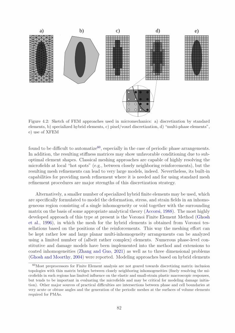
a) b) c) d) e)

Figure 4.2: Sketch of FEM approaches used in micromechanics: a) discretization by standardelements, b) specialized hybrid elements, c) pixel/voxel discretization, d) “multi-phase elements”,e) use of XFEM

found to be difficult to automatize60, especially in the case of periodic phase arrangements.In addition, the resulting stiffness matrices may show unfavorable conditioning due to sub-optimal element shapes. Classical meshing approaches are capable of highly resolving themicrofields at local “hot spots” (e.g., between closely neighboring reinforcements), but theresulting mesh refinements can lead to very large models, indeed. Nevertheless, its built-incapabilities for providing mesh refinement where it is needed and for using standard meshrefinement procedures are major strengths of this discretization strategy.

Alternatively, a smaller number of specialized hybrid finite elements may be used, whichare specifically formulated to model the deformation, stress, and strain fields in an inhomo-geneous region consisting of a single inhomogeneity or void together with the surroundingmatrix on the basis of some appropriate analytical theory (Accorsi, 1988). The most highlydeveloped approach of this type at present is the Voronoi Finite Element Method (Ghoshet al., 1996), in which the mesh for the hybrid elements is obtained from Voronoi tes-sellations based on the positions of the reinforcements. This way the meshing effort canbe kept rather low and large planar multi-inhomogeneity arrangements can be analyzedusing a limited number of (albeit rather complex) elements. Numerous phase-level con-stitutive and damage models have been implemented into the method and extensions tocoated inhomogeneities (Zhang and Guo, 2021) as well as to three dimensional problems(Ghosh and Moorthy, 2004) were reported. Modeling approaches based on hybrid elements

60Most preprocessors for Finite Element analysis are not geared towards discretizing matrix–inclusiontopologies with thin matrix bridges between closely neighboring inhomogeneities (finely resolving the mi-crofields in such regions has limited influence on the elastic and small-strain plastic macroscopic responses,but tends to be important in evaluating the microfields and may be critical for modeling damage initia-tion). Other major sources of practical difficulties are intersections between phase and cell boundaries atvery acute or obtuse angles and the generation of the periodic meshes at the surfaces of volume elementsrequired for PMAs.

82

are specifically tailored to inhomogeneous materials with matrix–inclusion topologies, andgood accuracy as well as significant gains in efficiency have been claimed for them.

A computational strategy that occupies a position between the above two approachesuses static condensation to remove the degrees of freedom of the interior nodes of the inho-mogeneities (or, in the case of coated reinforcements, of inhomogeneities plus interphases)from the stiffness matrix of a heterogeneous volume element (Liu et al., 2005a), the matrixregion being meshed by standard elements. Such methods may considerably reduce thecomputational requirements of linear multi-inhomogeneity models.

Especially when the phase arrangements to be studied are based on digital images ofactual microgeometries, a third approach to discretizing microgeometries is of interest. Itinvolves using a mesh consisting of regular, rectangular or hexahedral, elements of fixedsize having the same resolution as the digital data, each element being assigned to one ofthe constituents by operations such as thresholding of the grey values of the correspondingpixel or voxel. The use of structured meshes in such “digital image based” (DIB) modelshas the advantage of allowing an automatic, relatively straightforward model generationfrom appropriate experimental data (metallographic sections, tomographic scans) and ofavoiding ambiguities in smoothing the digital data (which are generally present if “stan-dard”, unstructured FE meshes are employed for discretizing pixel- or voxel-based data ofthis type). However, modeling approaches that directly discretize pixel or voxel geome-tries obviously lead to ragged phase boundaries, which may give rise to some oscillatorybehavior of the solutions (Niebur et al., 1999), can cause high local stress maxima (Teradaet al., 1997), may degrade accuracy, and negate detailed modeling of interfacial effects.Because the resolution of the microgeometry is determined by the chosen voxel size, meshsize control tends to be a difficult issue with DIB models, with global mesh refinementby supersampling tending to be an inefficient approach. Some of these limitations can,however, be addressed by local smoothing algorithms, compare Boyd and Muller (2006).Despite the above concerns, pixel- or voxel-based models have been claimed not to causeunacceptably large errors in the predicted macroscopic behavior even for relatively coarsediscretizations, at least in the linear elastic range (Guldberg et al., 1998), where they havefound wide use. In nonlinear regimes, however, local stress concentrations at ragged inter-faces may give rise to considerable errors which can be attenuated by averaging procedures,compare Fang et al. (2016).

When volume elements with matrix–inclusion topology are studied by voxel-basedmethods, care may be required to ensure that closely neighboring inhomogeneities areproperly resolved by the structured mesh and that their spurious “merging” is avoided.Many limitations of voxel-based Finite Element models also tend to apply to FFT-basedmicromechanical methods, which also make use of highly regular, structured, spatial dis-cretizations.

A fourth, related approach also uses structured FE meshes, but assigns phase prop-erties at the integration point level of standard elements (“multi-phase elements”), see,e.g., Schmauder et al. (1996) or Quilici and Cailletaud (1999). Essentially, this amounts totrading off the ragged boundaries caused by the voxel mesh against smeared-out (and typ-ically degraded) microfields within any element that contains a phase boundary, standard

83

FE shape functions being of limited suitability for handling stress or strain discontinuitieswithin elements. With respect to the element stiffnesses the latter concern can be coun-tered by overintegrating elements containing phase boundaries, which leads to improvedapproximations of integrals involving non-smooth displacements by numerical quadrature,see Zohdi and Wriggers (2001). The resulting stress and strain distributions, however, re-main smeared-out approximations in elements that contain phase boundaries. Multi-phaseelement models are, accordingly, also limited in their capabilities for detailed modeling ofinterfaces. An alternative technique giving rise to a similar pattern of strengths and limita-tions consists in prescribing suitably modified material properties to all elements containinga phase boundary (Toulemonde et al., 2008). In a recent development, “composite voxel”techniques (Kabel et al., 2017; Mareau and Robert, 2017) have been introduced within theframework of FFT-based homogenization, stiffnesses in both linear and nonlinear regimesbeing approximated in a consistent way, e.g., via laminate models.

The idea of reducing the considerable effort implied in classical meshing approaches hasled to applying a number additional of Finite Element modeling techniques to continuummicromechanics that make use of structured “base meshes” which are suitably modified forhandling inhomogeneous phase arrangements61. Strategies of this type have been based onthe Extended Finite Element method (XFEM) or the Generalized Finite Element Method(GFEM), phase boundaries that pass through individual elements being handled via ap-propriately enriched, non-smooth shape functions, see, e.g., Moes et al. (2003), Legrainet al. (2011), Soghrati et al. (2012) and Dunant et al. (2013). The resulting models canclosely follow the shapes of phase boundaries, compare the sketch in fig. 4.2e, and aresubject to few restrictions in terms of microgeometries that can be handled.

In addition, there are some FE-based micromechanical methods that do not fall withinthe groups shown in fig. 4.2. Among them are “embedded element” (“embedded mesh”,“embedded reinforcement”) or “domain superposition” techniques, which aim at reducingmodeling and computational costs by avoiding conformal meshing of individual reinforce-ments. Such approaches use a typically structured and often relatively coarse mesh ofcontinuum elements (“host mesh”) for the matrix. This is combined with truss or beamelements, see, e.g., Harper et al. (2012a), solid elements, compare, e.g., Jiang et al. (2008),or shell elements, see, e.g., Matveeva et al. (2014), that represent the inhomogeneities,the nodes of which do not, in general, coincide with those of the host mesh. These ele-ments describing the reinforcement are superposed over the host mesh, the different partsof the model being tied together, e.g., via appropriate extended FE formulations (Radtkeet al., 2011) or by constraint equations 62. Embedded reinforcement modeling strategiesimply the presence of excess volume in the models (“volume redundancy”), giving riseto a tendency towards overestimating the overall stiffness, especially at non-dilute vol-ume fractions, which, however, can be compensated for in many cases, compare Hoffmann(2012). Such approaches can markedly reduce the meshing and computational effort inFE-based micromechanical analysis, allowing very complex fiber–matrix configurations to

61It is not clear, however, to what extent structured and voxel-type meshes introduce a systematic biasinto the orientation of regions of elevated strain in highly loaded, nonlinear regimes.

62Embedded element techniques were originally developed for modeling rebars in reinforced concretestructures.

84

be handled63. The resolution in terms of local displacement, strain and stress fields isclosely tied to the pertinent capabilities of the host mesh, tending to limit the accuracyachievable with such models; this can be counteracted by enriching the shape functionsof appropriate matrix elements and/or by adaptive mesh refinement, compare Goudarziand Simone (2019). A different FE-based approach to studying composites reinforced bylong fibers that are neither straight nor aligned can be based on modeling the latter by“strings” of volume elements and filling the matrix space in-between by a suitable volumemesh (Fliegener et al., 2014). Again, local resolution of the microfields is traded off againstthe capability of handling complex fiber reinforcement geometries.

A relatively recent development for studying microgeometries involving large numbersof inhomogeneities (hundreds to thousands) by Finite Element methods involves finite el-ement programs specially geared towards solving micromechanical problems. Such codesmay make use, e.g., of matrix-free iterative solvers such as Conjugate Gradient (CG)methods, analytical solutions for the microfields (such as constant strain approximationscorresponding to the upper Hill bounds, eqn. (3.1), being employed as starting solutionsto speed up convergence64). For micromechanical studies involving such solvers see, e.g.,Gusev (1997), Zohdi and Wriggers (2001) or Arbenz et al. (2008). An alternative approachin this context are multi-grid solvers, compare, e.g., Gu et al. (2016). Very fast solvershave opened the possibility of handling very large volume elements or inverse problems,e.g., for finding optimal particle shapes for given load cases and damage modes (Zohdi,2003). Further increases in efficiency can be achieved for very large voxel-based linear DIBmodels by exploiting the fact that, in the case of linear analysis, all elements pertaining toa given phase have identical element stiffness matrices.

Special Finite Element formulations (and dedicated FE programs) have been requiredin many cases for asymptotic homogenization models, compare section 5.3, and for otherschemes that concurrently solve the macroscopic and microscopic problems, compare Ur-banski (1999).

A further, relatively recent numerical approach that is related to FE methods are re-duced basis (or reduced order) homogenization schemes, see, e.g., Fritzen and Kunc (2018),which use globally supported trial and weighting functions to obtain much smaller alge-braic systems. Appropriately choosing such functions and performing efficient numericalintegration on them are important issues for such reduced order methods. The Nonuni-form Transformation Analysis mentioned earlier was among the first methods of this type.Another recent strategy for generating computationally less demanding models makes useof soft computing methods such as neural networks (Kim et al., 2021). Like reduced or-der schemes, such approaches require considerable up-front effort which typically involves“classical” numerically-based models.

Discrete microstructure approaches employing numerical engineering methods are bestsuited to studying phase arrangements in which the characteristic lengths of the important

63Reinforcements approximated by rigid, one-dimensional objects are referred to as rigid line inclusions;they show some interesting properties, compare Wang et al. (1985).

64Essentially, in such a scheme the initial guess gives a reasonable estimate of “long wavelength” contri-butions to the solution, and the CG iterations take care of “short wavelength” variations.

85

geometrical features do not differ excessively. If this is not the case, e.g., for randomlyoriented inhomogeneities of high aspect ratio, very large volume elements may be required,meshing may become onerous, and the numerical effort for solving the models may be-come very high, especially for three-dimensional configurations. For methods making useof structured meshes, such as FFT algorithms and FE-based voxel models, the chosenmesh or voxel size intrinsically limits the achievable geometrical resolution. In the case ofapproaches that employ unstructured meshes and support local mesh refinement, such asstandard FE methods in the sense of figure 4.2, practical limits on resolution tend to beimposed by the size and conditioning of the resulting systems of algebraic equations. Forexample, discrete microstructure models of composites reinforced by polydispersely sizedparticles the diameters of which differ by more than, say, an order of magnitude tend tobecome very unwieldy; similar difficulties arise when modeling inhomogeneities with thincoatings. Another issue requiring special precautions is the handling of extremely closelyspaced or touching reinforcements numerically-based full field models65, compare, e.g., Gu-sev (2016); such geometrical features may be of considerable importance to the damagebehavior of composites, see, e.g., (Grufman and Ellyin, 2008).

Under conditions of macroscopic softening, e.g., due to damage or localization, dis-cretizing methods are liable to producing mesh-dependent results. Such tendencies maybe counteracted by appropriate regularization procedures, among them enrichment withhigher-order gradients, see e.g., Geers et al. (2001a), nonlocal averaging of the rate ofan appropriate internal variable, compare, e.g., Jirasek and Rolshoven (2003), the use oftime dependent formulations involving rate effects, see, e.g., Needleman (1987), or localaveraging, compare, e.g., Fang et al. (2016).

4.4 Evaluation of Results

When linear elastic or thermoelastic inhomogeneous materials are studied, the aim of ho-mogenization in full field approaches consists in evaluating the effective elasticity tensors,E∗, and thermal expansion tensors, α∗, or (some of) the pertinent moduli. In homoge-nization studies involving nonlinear, path-dependent constituent behavior, e.g., elastoplas-ticity, thermoelastoplasticity, viscoelastoplasticity or damage no solutions of a generalitycomparable to that of the above tensors exist. Here, typically the evolution of appropriatemacroscopic variables is followed along some specified load path, e.g., in the form of effec-tive stress–strain relations66.

In linear elastic homogenization it is typically preferable to solve for the macroscopicelastic tensors, which automatically provide full information on the macroscopic elasticsymmetry of the volume element, rather than reconstructing them from results on individ-

65Strict two-phase configurations may, in fact, constitute a considerable idealization for the regions closeto touching (“percolating”) or nearly touching inhomogeneities. On the one hand, production processesmay give rise to preferential accumulation of pores and impurities at such positions in actual materials.On the other hand, it is not clear to what extent point contact between neighboring inhomogeneities is aphysically reasonable model.

66Homogenized tangent tensors may also be evaluated for given load states, compare, e.g., (Ghosh et al.,1996). This is of special interest in hierarchical and multi-scale analysis employing discrete microstructuremodels as implicit material models for Finite Element models on the macroscale.

86

ual moduli67. For three-dimensional configurations, six linearly independent mechanicalload cases must be applied to the volume element for evaluating macroscopic elastic ten-sors, and a homogeneous temperature change is required for obtaining the macroscopicthermal expansion tensor. The effective elastic tensors of inhomogeneous materials withorthotropic or higher symmetry show similar structures to those of isotropic symmetry,see eqns. (1.12) and (1.13), i.e., in Voigt/Nye notation all tensor elements are zero withthe exception of the upper left submatrix and the diagonal of the lower right submatrix.In contrast, volume elements obtained from real structures or generated with stochastics-based models are typically too small to be proper RVEs and, accordingly, give rise tohomogenized tensors that show small contributions from lower elastic symmetries, typi-cally making them triclinc (Karimi et al., 2020). In addition, minor perturbations due toroundoff errors may be present. Evidently, volume elements aimed at describing statisti-cally isotropic, transversely isotropic or orthotropic material behavior must be expected toactually return lower macroscopic material symmetries.

Such deviations from an “elastic target symmetry”, which tend to decrease with grow-ing size (and number, if ensemble averaging is used) of SVEs used (Harper et al., 2012b),can be mitigated to some extent by finding the elastic tensor of the required symmetry thatis closest to the “raw” elastic tensor obtained from homogenization and averaging. Pahrand Bohm (2008) proposed a simplified approach in which this raw elastic tensor obtainedfrom an SVE of the type shown in fig. 5.4 (which aims at describing a statistically isotropiccomposite) is first projected onto an orthotropic base68. Closest isotropic tensors can thenbe obtained as the isotropic term of a generalized spherical harmonics expansion, using aprocedure developed by He and Curnier (1997). Alternatively, expressions resulting fromthe minimization of an appropriately defined distance between an elasticity tensor of pre-scribed symmetry and a given anisotropic elasticity tensor, as discussed by Norris (2006),Moakher and Norris (2006) as well as Bucataru and Slawinski (2009), may be used for find-ing the closest isotropic, cubic or transversally isotropic elasticity tensors. Such procedureshave been successfully applied to evaluating effective moduli pertaining to macroscopicallyisotropic elastic behavior from ensemble averaged sets of SVEs by Rasool and Bohm (2012),giving excellent agreement with the three-point estimates of Torquato (1997, 1998a) forrandomly positioned, non-interpenetrating, identical spherical reinforcements. Alternativeways for extracting elasticity tensors of the required macroscopic symmetry consist, on theone hand, of rotational averaging for obtaining isotropic or transversally isotropic effectiveelastic behavior and, on the other hand, of projection to appropriate tensor bases. Forstudies involving isotropic averaging in such a context see, e.g., Cook and Young (1985)or Gusev (2016), and for transversally isotropic averaging compare, e.g., Aboudi (1987).Even though such methods can be highly useful in SVE-based homogenization, they areof an inherently ad-hoc character.

67Ensemble averaging over a number of SVEs also is arguably best done in terms of the elastic tensors.Furthermore, if load-controlled periodic homogenization is used, elastic tensors can be obtained at moderatecost because solutions for the required linearly independent load vectors can be found cheaply once thesystem matrix has been factorized.

68Actually, in finding the orthotropic elasticity tensor that is closest to a raw elastic tensor the orienta-tions of the former’s principal axes should also be considered. In raw elastic tensors obtained by periodichomogenization from reasonably large volume elements typically only relatively small deviations from thetarget symmetry are present, whereas results from windowing methods, compare chapter 6, using smallvolume elements may lead to more pronounced deviations from the expected macroscopic elastic symmetry.

87

In micromechanical applications numerical engineering methods directly evaluate themicroscopic fields, i.e., for mechanical analyses, the fluctuating displacements, stresses andstrains as well as fields derived from them. In the case of displacement-based FE methodsusing isoparametric elements, the microscopic stresses and strains are primarily evaluatedat the integration point level of the individual elements, nodal values being obtained byextrapolation and averaging procedures. Some care, however, is necessary in using suchdata, because the extreme values of microscopic stresses and strains may depend markedlyon details of the microgeometry, of the discretization used and, in the case of nodal data,of the evaluation procedure. Furthermore, idiosyncrasies of the numerical methods maycome into play, one case being the reduced accuracy of stress and strain fields obtainedby displacement-based FE methods at interfaces between constituents and at the models’surfaces compared to the interior of regions occupied by a given phase.

For evaluating volume averages of stress- and strain-like variables from numerical pre-dictions for microscopic fields in a small strain setting, it is typically good practice to usedirect volume integration on the basis of eqn. (1.16)69. Many FE codes provide the datanecessary for approximating volume averaging by approximate numerical quadrature,

〈f〉 =1

Ω

∫

Ω

f(z)dΩ ≈ 1

Ω

Ni∑

l=1

fl Ωl . (4.8)

Here fl and Ωl are the function value and the integration weight (in terms of the volumeof the integration point), respectively, associated with the l-th integration point within agiven integration volume Ω that contains Ni integration points. By analogy, the standarddeviation of function f(z) over volume Ω can be evaluated as70

S(f) ≈

√√√√ 1

Ω

Ni∑

l=1

(fl − 〈f〉)2 Ωl . (4.9)

If the volumes associated with integration points are not available a simplified version ofeqn. (4.8),

〈f〉 ≈ 1

Ω

Ne∑

n=1

fn Ωn , (4.10)

69It is of practical interest that volume averaged and phase averaged microfields obtained from fullfield analysis must fulfill all relations given in section 2.1; this can be conveniently used to check theconsistency of a given model by inserting appropriate results into eqns. (2.5). Note, however, that in thefinite deformation regime appropriate stress and strain measures must be used for this purpose. Whereasthe volume averaged nominal stress can generally be obtained via eqns. (1.3) and (4.8), this does not holdfor the Cauchy stress (Hill, 1972; Nemat-Nasser, 1999). In fact, volume averaging of stress and straintensors in the finite strain regime is not necessarily possible, compare, e.g., Kouznetsova et al. (2002). Ifeqn. (4.8) or equivalents are to be used for such a purpose, special care as well as knowledge of the stressand strain measures actually used by the FE code are required.

70Procedures analogous to eqns. (4.8) and (4.9) may also be used for evaluating other volume integrals,e.g., in computing Weibull-type fracture probabilities for reinforcement particles or fibers (Antretter, 1998;Bohm et al., 2002).

88

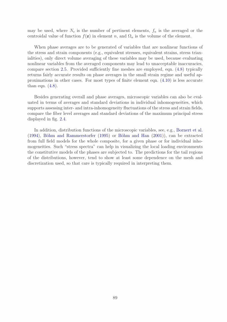
may be used, where Ne is the number of pertinent elements, fn is the averaged or thecentroidal value of function f(z) in element n, and Ωn is the volume of the element.

When phase averages are to be generated of variables that are nonlinear functions ofthe stress and strain components (e.g., equivalent stresses, equivalent strains, stress triax-ialities), only direct volume averaging of these variables may be used, because evaluatingnonlinear variables from the averaged components may lead to unacceptable inaccuracies,compare section 2.5. Provided sufficiently fine meshes are employed, eqn. (4.8) typicallyreturns fairly accurate results on phase averages in the small strain regime and useful ap-proximations in other cases. For most types of finite element eqn. (4.10) is less accuratethan eqn. (4.8).

Besides generating overall and phase averages, microscopic variables can also be eval-uated in terms of averages and standard deviations in individual inhomogeneities, whichsupports assessing inter- and intra-inhomogeneity fluctuations of the stress and strain fields,compare the fiber level averages and standard deviations of the maximum principal stressdisplayed in fig. 2.4.

In addition, distribution functions of the microscopic variables, see, e.g., Bornert et al.(1994), Bohm and Rammerstorfer (1995) or Bohm and Han (2001)), can be extractedfrom full field models for the whole composite, for a given phase or for individual inho-mogeneities. Such “stress spectra” can help in visualizing the local loading environmentsthe constitutive models of the phases are subjected to. The predictions for the tail regionsof the distributions, however, tend to show at least some dependence on the mesh anddiscretization used, so that care is typically required in interpreting them.

89

Chapter 5

Periodic Microfield Approaches

Periodic Microfield Approaches (PMAs) aim at approximating the macroscopic and micro-scopic behavior of inhomogeneous materials by studying model materials that have periodicmicrostructures.

5.1 Basic Concepts of Periodic Homogenization

Periodic microfield approaches analyze the behavior of infinite (one, two- or three-dimensio-nal) periodic phase arrangements under the action of far field mechanical loads or uniformtemperature fields71, for which the Hill–Mandel criterion can be fulfilled as discussed insection 4.2. The most common approach to studying the stress and strain fields in such pe-riodic configurations is based on describing the microgeometry by a periodically repeatingunit cell72 (RUC), to which the investigations may be limited without loss of informationor generality, at least for static analysis73.

71Standard PMAs cannot handle macroscopic gradients in mechanical loads, temperature or compositionin any direction in which periodicity of the fields is prescribed. Such gradients or boundaries can be studied,however, in directions where periodicity is not prescribed, a typical case being layer-type models that arenon-periodic in one direction and periodic in the other(s), see, e.g., Wittig and Allen (1994), Reiter et al.(1997) and Weissenbek et al. (1997).

72In the present report the designation “unit cell” is used for any volume element that can generatea periodic microgeometry. Accordingly, a unit cell may comprise a simple periodic base unit (or part ofit), a collective of simple periodic base units, or a phase arrangement of arbitrary geometrical complexity(multi-fiber or multi-particle unit cell) that shows translational periodicity; in the limiting case a unit cellmay thus be a proper representative volume element. Accordingly, the discussion of volume element sizesin section 4.1 is fully pertinent to unit cell models.

73Periodic phase arrangements are not very well suited to modeling the transient behaviors of structuralcomposite materials. In dynamic settings, RUC act as phononic crystals, i.e., as metamaterials exhibitingphononic band structures and dispersion relations. Studying such behavior, however, is a research field inits own right, compare, e.g., Hussein et al. (2014), in which periodic volume elements play an importantrole, see, e.g., Suzuki and Yu (1998).Unit cells are typically limited to describing wavelengths smaller than or equal to their relevant dimension,which is a direct consequence of the boundary conditions required for obtaining periodicity. By analogy,in stability analysis of inhomogeneous materials RUCs can directly resolve only buckling modes of specificwavelengths, so that considerable care is required in using them, compare Vonach (2001) or Pahr andRammerstorfer (2006). However, bifurcation modes with wavelengths exceeding the size of the unit cellcan be handled via periodic linear models by using the Bloch theorem (Gong et al., 2005).

90

The literature on periodic homogenization of inhomogeneous materials is fairly exten-sive, and well developed mathematical theories are available on scale transitions in periodicstructures and materials, compare Michel et al. (2001). A wide variety of unit cells havebeen employed in such studies, ranging from geometries that describe simple periodic arrays(“lattices”) of inhomogeneities to complex periodic phase arrangements, such as volumeelements containing considerable numbers of statistically arranged inhomogeneities. Forsome simple periodic phase arrangements and for linear material behavior it has provenpossible to find analytical solutions based on series expansions making direct use of the pe-riodicity (Sangani and Lu, 1987; Wang et al., 2000; Cohen, 2004; Drago and Pindera, 2008).

Even though most PMA studies in the literature have used standard numerical engineer-ing methods as discussed in section 4.3, some other numerical schemes have been proposedthat are specialized to periodic phase arrangements. One of them, known as the Method ofCells (Aboudi, 1989, 1991), in its basic form discretizes unit cells that correspond to squarearrangements of square fibers into four subcells, within each of which displacements areapproximated by low-order polynomials. Traction and displacement continuity conditionsat the faces of the subcells are imposed in an average sense and analytical and/or semi-analytical approximations to the deformation fields are obtained in the elastic and inelasticranges. Because they use highly idealized microgeometries, provide only limited informa-tion on the microscopic stress and strain fields, and have limited capabilities for handlingaxial shear, the resulting models pose relatively low computational requirements and canprovide constitutive descriptions for analyzing structures made of continuously reinforcedcomposites, see, e.g., Arenburg and Reddy (1991). Developments of the algorithm led tothe Generalized Method of Cells (Aboudi, 1996), which is more flexible geometrically andallows finer discretizations of unit cells for fiber and particle reinforced composites, rein-forcement and matrix being essentially split into a number of “subregions” of rectangularor hexahedral shape. For some comparisons with microfields obtained by Finite Elementbased unit cells see, e.g., Iyer et al. (2000) or Pahr and Arnold (2002). Later, higher orderdisplacement interpolants were brought in to obtain the High-Fidelity Generalized Methodof Cells (Aboudi, 2004), which provides an alternative to Finite Element algorithms for“pixel element” micromechanical models (compare section 4.3). This method was also ex-tended to general quadrilateral cell shapes (Haj-Ali and Aboudi, 2010).

A further group of solution strategies for PMAs reported in the literature (Axelsen andPyrz, 1995; Fond et al., 2001; Schjødt-Thomsen and Pyrz, 2004) use numerically evaluatedequivalent inclusion approaches that account for interacting inhomogeneities as provided,e.g., by the work of Moschovidis and Mura (1975). Alternatively, multipole expansionmethods can handle complex periodic matrix–inclusion microgeometries (Sangani and Mo,1997; Kushch et al., 2008; Kushch, 2013). Furthermore, the elastic fields in periodic inho-mogeneous materials can be evaluated numerically via variational methods for determiningstress-free strain fields (Wang et al., 2002).

As mentioned in section 1.5, periodic homogenization cannot be freely used for mod-eling damage in and failure of inhomogeneous materials, all relevant geometrical features,among them crack patterns, being per definition periodic. Consequently, PMAs cannotdescribe behavior involving macroscopic localization of damage, failure in periodic modelsrather being akin to some kind of fragmentation. This, however, does not rule out the use

91

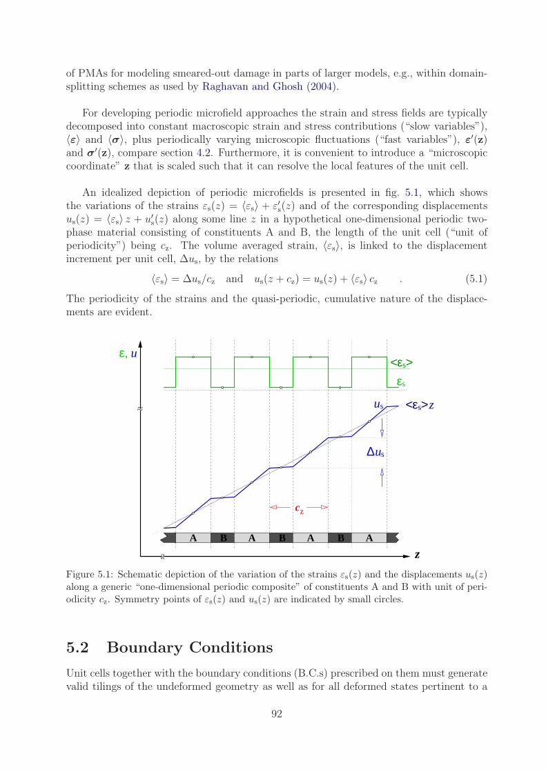
of PMAs for modeling smeared-out damage in parts of larger models, e.g., within domain-splitting schemes as used by Raghavan and Ghosh (2004).

For developing periodic microfield approaches the strain and stress fields are typicallydecomposed into constant macroscopic strain and stress contributions (“slow variables”),〈ε〉 and 〈σ〉, plus periodically varying microscopic fluctuations (“fast variables”), ε′(z)and σ′(z), compare section 4.2. Furthermore, it is convenient to introduce a “microscopiccoordinate” z that is scaled such that it can resolve the local features of the unit cell.

An idealized depiction of periodic microfields is presented in fig. 5.1, which showsthe variations of the strains εs(z) = 〈εs〉 + ε′s(z) and of the corresponding displacementsus(z) = 〈εs〉 z + u′s(z) along some line z in a hypothetical one-dimensional periodic two-phase material consisting of constituents A and B, the length of the unit cell (“unit ofperiodicity”) being cz. The volume averaged strain, 〈εs〉, is linked to the displacementincrement per unit cell, ∆us, by the relations

〈εs〉 = ∆us/cz and us(z + cz) = us(z) + 〈εs〉 cz . (5.1)

The periodicity of the strains and the quasi-periodic, cumulative nature of the displace-ments are evident.

uε,

<ε >

ε<ε >

u z

zA A AB B B A

s

s

s

s

∆us

cz

Figure 5.1: Schematic depiction of the variation of the strains εs(z) and the displacements us(z)along a generic “one-dimensional periodic composite” of constituents A and B with unit of peri-odicity cz. Symmetry points of εs(z) and us(z) are indicated by small circles.

5.2 Boundary Conditions

Unit cells together with the boundary conditions (B.C.s) prescribed on them must generatevalid tilings of the undeformed geometry as well as for all deformed states pertinent to a

92

given micromechanical problem. Accordingly, gaps and overlaps between neighboring vol-ume elements as well as unphysical constraints on their deformations must not be allowed,i.e., the cells must be geometrically compatible. In order to achieve this, the boundaryconditions for the unit cells must be specified in such a way that all deformation modesappropriate for the load cases to be studied can be attained. The major types of boundaryconditions used in periodic microfield analysis are periodicity, symmetry, and antisymme-try B.C.s74. In PMA models one of these three types of boundary conditions must be usedfor any subset of any exterior boundary (unless it is a free boundary) of the volume ele-ment, irrespective of the numerical method employed for solving the equilibrium equations.

Generally, for any given periodic phase arrangement unit cells are non-unique, the rangeof possible shapes being especially wide when point or mirror symmetries are present inthe microgeometry (as tends to be the case for regular lattices). As an example, fig. 5.2depicts a (two-dimensional) periodic hexagonal array of circular inhomogeneities (e.g.,fibers oriented normally to the plane) and some of the unit cells that can be used to studyaspects of the behavior of this phase arrangement. There are considerable differences inthe sizes and capabilities of the unit cells shown.

2

1 periodic boundarysymmetry boundarypoint symmetry boundary

symmetry center(pivot point)

AB

F

GC

H I

D

E

J

Figure 5.2: Periodic hexagonal array of circular inhomogeneities in a matrix and 10 unit cells or“reduced cells” that can be used to describe the mechanical responses of this arrangement underloads acting parallel to the coordinate axes.

Periodicity Boundary Conditions

The most general boundary conditions for volume elements in periodic homogenizationare periodicity (periodic fluctuation, “toroidal”, “cyclic”) B.C.s, which can handle anyphysically valid deformation state of the unit cell and, consequently, of the inhomogeneous

74For more formal treatments of boundary conditions for unit cells than given here see, e.g., Anthoine(1995) or Michel et al. (1999).

93

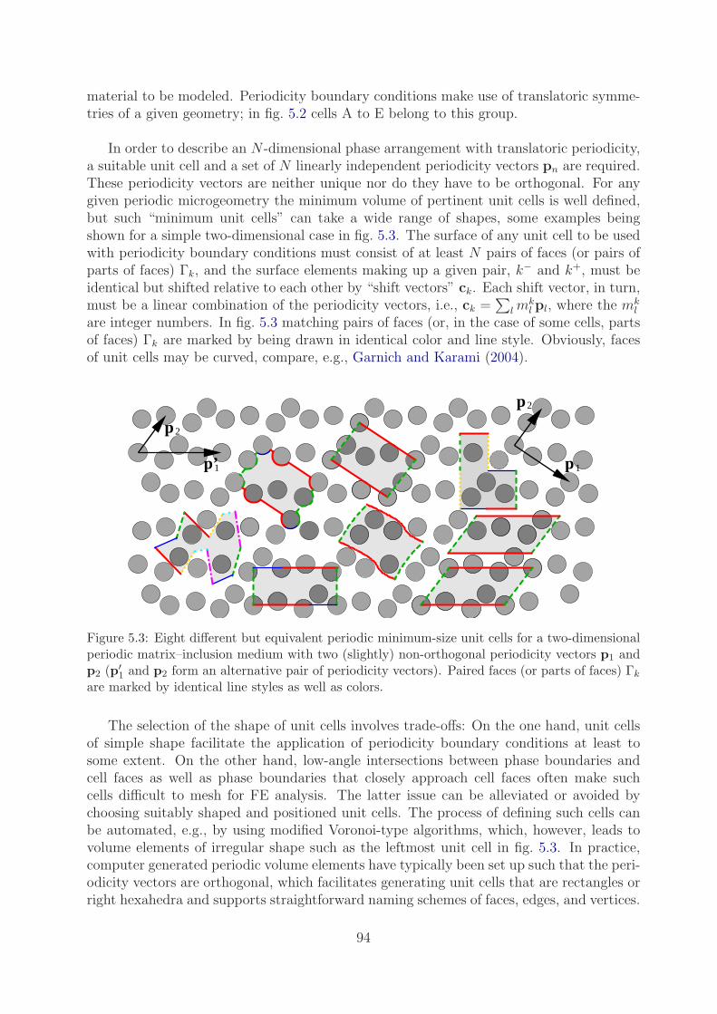
material to be modeled. Periodicity boundary conditions make use of translatoric symme-tries of a given geometry; in fig. 5.2 cells A to E belong to this group.

In order to describe an N -dimensional phase arrangement with translatoric periodicity,a suitable unit cell and a set of N linearly independent periodicity vectors pn are required.These periodicity vectors are neither unique nor do they have to be orthogonal. For anygiven periodic microgeometry the minimum volume of pertinent unit cells is well defined,but such “minimum unit cells” can take a wide range of shapes, some examples beingshown for a simple two-dimensional case in fig. 5.3. The surface of any unit cell to be usedwith periodicity boundary conditions must consist of at least N pairs of faces (or pairs ofparts of faces) Γk, and the surface elements making up a given pair, k− and k+, must beidentical but shifted relative to each other by “shift vectors” ck. Each shift vector, in turn,must be a linear combination of the periodicity vectors, i.e., ck =

∑lm

kl pl, where the mk

l

are integer numbers. In fig. 5.3 matching pairs of faces (or, in the case of some cells, partsof faces) Γk are marked by being drawn in identical color and line style. Obviously, facesof unit cells may be curved, compare, e.g., Garnich and Karami (2004).

2

p2

1p

p

p’1

Figure 5.3: Eight different but equivalent periodic minimum-size unit cells for a two-dimensionalperiodic matrix–inclusion medium with two (slightly) non-orthogonal periodicity vectors p1 andp2 (p′

1 and p2 form an alternative pair of periodicity vectors). Paired faces (or parts of faces) Γk

are marked by identical line styles as well as colors.

The selection of the shape of unit cells involves trade-offs: On the one hand, unit cellsof simple shape facilitate the application of periodicity boundary conditions at least tosome extent. On the other hand, low-angle intersections between phase boundaries andcell faces as well as phase boundaries that closely approach cell faces often make suchcells difficult to mesh for FE analysis. The latter issue can be alleviated or avoided bychoosing suitably shaped and positioned unit cells. The process of defining such cells canbe automated, e.g., by using modified Voronoi-type algorithms, which, however, leads tovolume elements of irregular shape such as the leftmost unit cell in fig. 5.3. In practice,computer generated periodic volume elements have typically been set up such that the peri-odicity vectors are orthogonal, which facilitates generating unit cells that are rectangles orright hexahedra and supports straightforward naming schemes of faces, edges, and vertices.

94

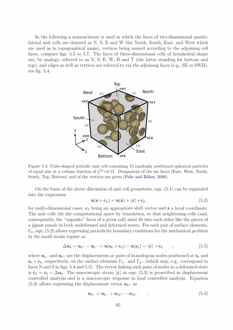
In the following a nomenclature is used in which the faces of two-dimensional quadri-lateral unit cells are denoted as N, S, E and W (for North, South, East, and West whichare used as in topographical maps), vertices being named according to the adjoining cellfaces, compare figs. 5.5 to 5.7. The faces of three-dimensional cells of hexahedral shapeare, by analogy, referred to as N, S, E, W, B and T (the latter standing for bottom andtop), and edges as well as vertices are referred to via the adjoining faces (e.g., SE or SWB),see fig. 5.4.

NEB

SEB

NWT

NET

SWB

SWT

WT

NE

NT

EBSB

SW

Figure 5.4: Cube-shaped periodic unit cell containing 15 randomly positioned spherical particlesof equal size at a volume fraction of ξ(i)=0.15. Designators of the six faces (East, West, North,South, Top, Bottom) and of the vertices are given (Pahr and Bohm, 2008).

On the basis of the above discussion of unit cell geometries, eqn. (5.1) can be expandedinto the expression

u(z + ck) = u(z) + 〈ε〉 ∗ ck (5.2)

for multi-dimensional cases, ck being an appropriate shift vector and z a local coordinate.The unit cells tile the computational space by translation, so that neighboring cells (and,consequently, the “opposite” faces of a given cell) must fit into each other like the pieces ofa jigsaw puzzle in both undeformed and deformed states. For each pair of surface elements,Γk, eqn. (5.2) allows expressing periodicity boundary conditions for the mechanical problemin the small strain regime as

∆uk = uk+ − uk− = u(sk + ck)− u(sk) = 〈ε〉 ∗ ck , (5.3)

where uk− and uk+ are the displacements at pairs of homologous nodes positioned at sk andsk + ck, respectively, on the surface elements Γk− and Γk+ (which may, e.g., correspond tofaces N and S in figs. 5.4 and 5.5). The vector linking such pairs of nodes in a deformed stateis ck = ck + ∆uk. The macroscopic strain 〈ε〉 in eqn. (5.3) is prescribed in displacementcontrolled analysis and is a macroscopic response in load controlled analysis. Equation(5.3) allows expressing the displacement vector uk+ as

uk+ = uk− + uM+ − uM− , (5.4)

95

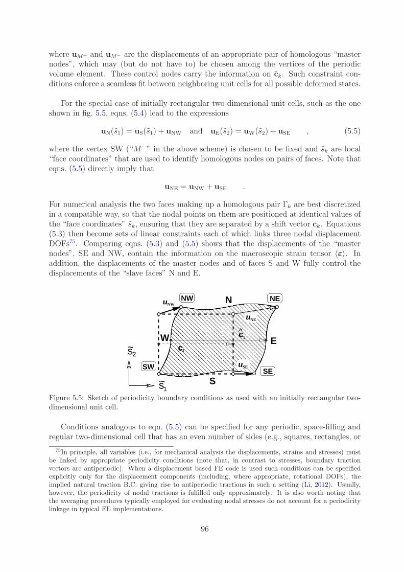
where uM+ and uM− are the displacements of an appropriate pair of homologous “masternodes”, which may (but do not have to) be chosen among the vertices of the periodicvolume element. These control nodes carry the information on ck. Such constraint con-ditions enforce a seamless fit between neighboring unit cells for all possible deformed states.

For the special case of initially rectangular two-dimensional unit cells, such as the oneshown in fig. 5.5, eqns. (5.4) lead to the expressions

uN(s1) = uS(s1) + uNW and uE(s2) = uW(s2) + uSE , (5.5)

where the vertex SW (“M−” in the above scheme) is chosen to be fixed and sk are local“face coordinates” that are used to identify homologous nodes on pairs of faces. Note thateqns. (5.5) directly imply that

uNE = uNW + uSE .

For numerical analysis the two faces making up a homologous pair Γk are best discretizedin a compatible way, so that the nodal points on them are positioned at identical values ofthe “face coordinates” sk, ensuring that they are separated by a shift vector ck. Equations(5.3) then become sets of linear constraints each of which links three nodal displacementDOFs75. Comparing eqns. (5.3) and (5.5) shows that the displacements of the “masternodes”, SE and NW, contain the information on the macroscopic strain tensor 〈ε〉. Inaddition, the displacements of the master nodes and of faces S and W fully control thedisplacements of the “slave faces” N and E.

NW

SE

NE

SW

NEu

SEu

s

c

c

N

W E

S

s

uNW

1~

1

^1

2~

Figure 5.5: Sketch of periodicity boundary conditions as used with an initially rectangular two-dimensional unit cell.

Conditions analogous to eqn. (5.5) can be specified for any periodic, space-filling andregular two-dimensional cell that has an even number of sides (e.g., squares, rectangles, or

75In principle, all variables (i.e., for mechanical analysis the displacements, strains and stresses) mustbe linked by appropriate periodicity conditions (note that, in contrast to stresses, boundary tractionvectors are antiperiodic). When a displacement based FE code is used such conditions can be specifiedexplicitly only for the displacement components (including, where appropriate, rotational DOFs), theimplied natural traction B.C. giving rise to antiperiodic tractions in such a setting (Li, 2012). Usually,however, the periodicity of nodal tractions is fulfilled only approximately. It is also worth noting thatthe averaging procedures typically employed for evaluating nodal stresses do not account for a periodicitylinkage in typical FE implementations.

96

hexagons) or three-dimensional cell that has an even number of faces (e.g., cubes, hexa-hedra, rhombic dodecahedra, or regular tetrakaidecahedra) arranged such that they formhomologous pairs. The scheme can also be extended to unit cells of less regular shape pro-vided their faces can be suitably paired off, compare Cruz and Patera (1995), Estrin et al.(1999) or Xia et al. (2003) as well as figs. 5.2 and 5.3. Periodicity B.C.s may be viewed as theleast restrictive option for multi-inhomogeneity unit cell models using phase arrangementsgenerated by statistics-based algorithms (see, however, Mesarovic and Padbidri (2005)).Compared to other discrete microstructure approaches, periodic homogenization typicallyshows the fastest convergence in terms of sizes of volume elements, see, e.g., El Houdaiguiet al. (2007). For further discussions of periodicity B.C. see, e.g., Garoz et al. (2019).

For layer-type models, which can be generated by specifying free surfaces at appro-priate pairs of boundaries, macroscopic rotational degrees of freedom, i.e., macroscopicbending and twisting, can be studied by appropriately modifying the standard periodicityB.C.s, eqns. (5.2) to (5.5), for the other faces. When such “structure-type” macroscopicrotational degrees of freedom are present, out-of-plane shear loads must be accompaniedby appropriate bending moments to achieve stress equilibrium, compare, e.g., Urbanski(1999). Models of this type allow using periodic homogenization for evaluating homog-enized “laminate stiffnesses” of inhomogeneous plates and shells for use within classicallamination theory (Jones, 1999), for details see, e.g., Pahr and Rammerstorfer (2006).

The above treatment can be carried over into the large strain regime. Periodicityboundary conditions that are conceptual developments of eqn. (5.5) can be devised forcases where standard conditions for homogenization are not met, gradient (nonlocal) the-ories are employed on the macroscale, and higher-order stresses as well as strain gradientsfigure in coupling the length scales (Geers et al., 2001b). The resulting deformation pat-terns of the cells, however, no longer follow geometrical compatibility as discussed above.

In practice FE-based studies of volume elements subjected to periodicity boundaryconditions can be somewhat expensive and some effort may be required for providing com-patible discretizations on periodic pairs of faces. Accordingly, there has been researchinterest in relaxing the compatibility requirements, see, e.g., Wippler et al. (2011), in im-plementing periodicity B.C. for non-compatible meshes via constraint equations, compare,e.g., Nguyen et al. (2012) or Wang et al. (2017), and in applying periodicity B.C. to non-periodic volume elements, see, e.g., Schneider et al. (2017). Such approximations typicallygive rise to some perturbations of the microfields at the cell boundaries in analogy to theboundary layers shown by windowing and embedding models, compare section 4.2. Forreasonably large volume elements such perturbations tend to show minor effects on thepredicted homogenized behavior in linear and weakly nonlinear regimes. For strongly non-linear local behaviors, such as phase-level damage, however, spurious local fields due toboundary perturbations may markedly influence the predicted macroscopic responses, evenfor volume elements that closely approach representativity for linear properties.

Finally, it is worth noting that high-quality discretizations of periodic volume ele-ments can be obtained with reasonable effort by employing preprocessors that supportthe automatic generation of compatible meshes on homologous faces, such as Netgen(https://ngsolve.org/).

97

Symmetry Boundary Conditions

For rectangular and hexahedral volume elements in which the faces of the unit cell coincidewith symmetry planes of the phase arrangement and for which this property is retainedfor all deformed states that are to be studied, periodicity B.C.s simplify to symmetry (ormirror) boundary conditions over a subset of the periodic volume, called a “reduced cell”in the following. Following the nomenclature of fig. 5.6 these B.C.s take the form

uE(s2) = uSE vN(s1) = vNW uW(s2) = 0 vS(s1) = 0 , (5.6)

where u and v stand for the displacement components in 1- and 2-direction, respectively.Equation (5.6) places constraints on the normal displacement components at the cells’surfaces, but leaves the tangential displacements free, thus enforcing the condition thatpairs of opposite faces must stay parallel throughout the deformation history. Accordingly,symmetry boundary conditions do not allow fluctuations of the local fields in directionsnormal to a given face of a unit cell or reduced cell76. Symmetry B.C.s pose no requirementswith respect to compatibility of phase arrangements or meshes at different faces, but theymay lead to undesirable shapes of inhomogeneities intersected by a cell face when theirmirror images are taken into account.

NW

SW

NE

SE

NEu

SEu

~s

s~EW

N

S

uNW

1

2

Figure 5.6: Sketch of symmetry boundary conditions as used with a rectangular two-dimensionalreduced cell.

Symmetry boundary conditions are fairly easy to use and tend to give rise to smallreduced cells for simply periodic phase arrangements. However, the load cases that canbe handled are limited to uniform thermal loads, mechanical loads that act in directionsnormal to one or more pairs of faces, and combinations of the above77. In fig. 5.2 cell Fuses boundary conditions of this type. Symmetry boundary conditions are typically highlyuseful for describing relatively simple microgeometries but may impose marked limitationson the geometries of complex phase arrangements.

76The stress and strain fluctuations ε′(z) and σ′(z) must obviously be symmetric with respect to sym-metry planes, whereas displacements accumulate across symmetry planes, compare fig. 5.1.

77Symmetry boundary conditions are compatible with uniaxial stress, uniaxial strain, extensional shear(obtained, e.g., in the two-dimensional case by applying normal stresses σa to the vertical and −σa tothe horizontal faces), hydrostatic and (hygro)thermal load cases. Accordingly, symmetry B.C.s are oftensufficient for materials characterization. However, the normal and shear stresses evaluated as above donot pertain to the same material coordinate system, extensional shear corresponds to pure shear in acoordinate system rotated by 45.

98

Antisymmetry Boundary Conditions

Antisymmetry (point symmetry, central reflection) boundary conditions require the pres-ence of centers of point symmetry (“pivot points”) and are, accordingly, even more limitedin terms of the microgeometries that they can handle. In contrast to symmetry boundaryconditions, however, unit cells employing antisymmetry B.C. on all faces are subject to fewrestrictions in terms of the load cases that can be handled. Among the volume elementsshown in fig. 5.2, cells G and H use point symmetry B.C.s on all faces and can handle anyin-plane deformation78. Alternatively, antisymmetry B.C.s can be combined with symme-try B.C.s to obtain very small reduced cells that are restricted to loads acting normal tothe symmetry faces, compare cells I and J in fig. 5.2. Figure 5.7 shows such a reduced cell,the antisymmetry boundary conditions being applied on face E where a pivot point P ispresent. For this configuration the boundary conditions

uU(sP) + uL(−sP) = 2uP

vN(s1) = vNW = 2vP vS(s1) = 0 uW(s2) = 0 , (5.7)

must be fulfilled, where uU(sP) and uL(−sP) are the displacement vectors of pairs of ho-mologous nodes U and L that are positioned symmetrically with respect to the pivot pointP. As indicated in fig. 5.7 the local coordinate system s is defined on face E and centered

SW

NWUu

Lu

~s

Pus~

W

S

NuNW

~s

SE

NE

E

L

U

P

1

2

p

Figure 5.7: Sketch of a quadrilateral two-dimensional reduced cell that combines antisymmetryboundary conditions on face E with symmetry boundary conditions on faces N, S and W.

on P. The undeformed geometry of such a face also must be antisymmetric with respect tothe pivot point P, and the phase arrangements as well as the discretizations on both halvesof face E must be compatible. Three-dimensional reduced cells employing combinations ofsymmetry and point symmetry B.C.s can, e.g., be used to advantage for studying cubicarrays of particles, see Weissenbek et al. (1994), or woven composites, compare Li and Zou(2011).

78Unit cells and reduced cells using antisymmetry boundary conditions may have odd numbers of faces.Triangular volume elements similar to cell H in fig. 5.2 were used, e.g., by Teply and Dvorak (1988) to studythe transverse mechanical behavior of hexagonal arrays of fibers. Rectangular cells with point symmetrieson each boundary were introduced by Marketz and Fischer (1994) for perturbed square arrangements ofinhomogeneities. The periodic cells D and E also show point symmetry on their faces.

99

For a reduced cell of the type shown in fig. 5.7, either the displacements of the masternodes SE and NW, uSE and uNW, or the displacements of the pivot P, uP, can be used forevaluating the macroscopic strain of the corresponding periodic model material, compareeqn. (5.17).

The description of real materials, which in general are not periodic, by periodic modelmaterials may entail some geometrical approximations. In the case of real structure geome-tries this may take the form of applying periodicity constraints to non-periodic geometriesor modifying the geometries such that they become periodic79. For periodic volume el-ements sufficiently large to approach proper RVEs the resulting errors in terms of thehomogenized responses will be of little practical relevance. However, perturbations of themicrofields in the vicinity of the cell surfaces will be present, which should be monitoredin the case of highly nonlinear analysis. In the linear range the use of windowing methodswith appropriate mixed boundary conditions, compare chapter 6, provides a superior al-ternative to ad-hoc “periodification” procedures.

Finally, it is worth noting that all of the above boundary conditions, eqns. (5.4), (5.5),(5.6) and (5.7) as well as their three-dimensional equivalents, can be handled by any FEcode that provides linear multipoint constraints between degrees of freedom and thus allowsthe linking of three or more DOFs by linear equations.

5.3 Application of Loads and Evaluation of Fields

Once suitable volume elements have been defined and appropriate boundary conditionsapplied, the appropriate loads in the form of uniform macroscopic stresses, uniform macro-scopic strains and/or homogeneous temperature excursions must be applied to link themicroscopic and macroscopic fields. Whereas loading by uniform temperature incrementsdoes not pose major difficulties, applying far field stresses or strains is not necessarilystraightforward. For example, the variations of the stresses along the faces of a unit cell ingeneral are not known a priori, so that it is not possible to prescribe the boundary tractionsvia distributed loads. There are two major approaches to implementing the micro–macrolinkage, both of which allow handling arbitrary stress or strain controlled load cases inlinear and nonlinear regimes.

Asymptotic Homogenization

The most versatile and elegant strategy for linking the macroscopic and microscopic fields inperiodic microfield models is based on a mathematical framework referred to as asymptotichomogenization, asymptotic expansion homogenization, or homogenization theory, see,e.g., Suquet (1987) or Auriault (2002). It is based on explicitly introducing macroscopicand microscopic coordinates, y and z, respectively, into the formulation of the problem.

79In the same vein, non-periodic, rectangular or cube-shaped volume elements may simply be subjectedto symmetry B.C. or may be mirrored with respect to two or three of their faces and then subjectedto periodicity B.C. These operations, however, may lead to undesirable shapes of reinforcements and tochanges in the phase arrangement statistics. Nevertheless, for sufficiently large multi-inhomogeneity cellsuseful results can be obtained with such a strategy, see, e.g., (Terada et al., 2000).

100

Microscopic and physical coordinates are linked by the expression

zi = xi/ǫ (5.8)

where ǫ = ℓ/L ≪ 1 is a scaling parameter. L and ℓ stand for the characteristic lengthsof the macro- and microscales80. The displacement field in the unit cell can then berepresented by an asymptotic expansion of the type

ui(y, z, ǫ) = u(0)i (y) + ǫ u

(1)i (y, z) + ǫ2 u

(2)i (y, z) + H.O.T. , (5.9)

where the u(0)i are the effective or macroscopic displacements and u

(1)i stands for the peri-

odically varying displacement fluctuations due to the microstructure81.

Using the chain rule, i.e.,

∂

∂xf(y(x), z(x), ǫ) → ∂

∂yf +

1

ǫ

∂

∂zf , (5.10)

in the small strain regime the strains can be related to the displacements as

εij(y, z, ǫ) =1

2

( ∂

∂yju(0)i +

∂

∂yiu(0)j

)+

(∂

∂zju(1)i +

∂

∂ziu(1)j

)

+ǫ

2

( ∂

∂yju(1)i +

∂

∂yiu(1)j

)+

(∂

∂zju(2)i +

∂

∂ziu(2)j

)+ H.O.T.

= ε(1)ij (y, z) + ǫ ε

(2)ij (y, z) + H.O.T. , (5.11)

where terms of the type ε(0)ij = 1

ǫ∂∂zju(0)i are deleted due to the underlying assumption that

the variations of slow variables are negligible at the microscale. By analogy the stressescan be expanded into the expression

σij(y, z, ǫ) = σ(1)ij (y, z) + ǫ σ

(2)ij (y, z) + H.O.T. . (5.12)

Using the two-scale assumption and, as a consequence, eqn. (5.10), the equilibrium equa-tions take the form

( ∂

∂yj+

1

ǫ

∂

∂zj

)σij(y, z, ǫ) + fi(y) = 0 , (5.13)

the fi being macroscopic body forces. By inserting eqn. (5.12) into this expression and sort-ing the resulting terms by order of ǫ a hierarchical system of partial differential equationsis obtained, the first two of which are

∂

∂zjσ(1)ij = 0 (order ǫ−1)

∂

∂yjσ(1)ij +

∂

∂zjσ(2)ij + fi = 0 (order ǫ0) . (5.14)

80Equation (5.8) may be viewed as “stretching” the microscale so it becomes comparable to themacroscale, f(x)→ f(y,y/ǫ) = f(y, z).

81The nomenclature used in eqns. (5.8) to (5.15) follows typical usage in asymptotic homogenization.It is more general than but can be directly compared to the one used in eqns. (1.2) to (5.7), where nomacroscopic coordinates y are employed.

101

The first of these equations gives rise to a boundary value problem at the unit cell level thatis referred to as the “micro equation”. By making a specific ansatz for the strains at themicrolevel and by volume averaging over the second equation in the system (5.14), whichis known as the “macro equation”, for elastic problems the microscopic and macroscopicfields can be linked such that the homogenized elasticity tensor, E∗

ijkl, is obtained as

E∗ijkl =

1

ΩUC

∫

ΩUC

Eijkl(z)[Iklmn +

∂

∂zlχkmn(z)

]dΩ . (5.15)

Here ΩUC is the volume of the unit cell, Eijkl(z) is the microscopic elasticity tensor, whichdepends on the constituent present at position z, Iijkl is the 4th-order unit tensor, and the“characteristic function” χkmn(z), a tensor of order 3, describes the deformation modes ofthe unit cell82 and, accordingly, relates the micro- and macrofields. Analogous expressionscan be derived for the tangent modulus tensors used in inelastic analysis, compare Ghoshet al. (1996).

The above relations can be used as the basis of Finite Element algorithms that solve forthe characteristic function χijk(z), a task that in most cases has required special analysiscodes. For detailed discussions of asymptotic homogenization methods within the frame-work of FEM-based micromechanics see, e.g., Hollister et al. (1991), Ghosh et al. (1996),Hassani and Hinton (1999), Chung et al. (2001) or Kanoute et al. (2009). Asymptotichomogenization procedures for elastic composites using commercial FE packages were pro-posed by a number of authors, among them Banks-Sills and Leiderman (1999), Barroqueiroet al. (2016), Colera and Kim (2019) and Christoff et al. (2020).

Asymptotic homogenization supports the direct coupling of FE models on the macro-and microscales, compare, e.g., Ghosh et al. (1996) or Terada et al. (2003), an approachthat has been used in a number of multi-scale studies (compare chapter 8); concurrentcoupling is sometimes referred to as the FE2 method (Feyel, 2003). A treatment of homog-enization in the vicinity of macroscopic boundaries can be found in Schrefler et al. (1997).Asymptotic homogenization schemes are suitably for handling finite strains and they havealso been employed for problems combining higher-order stresses and strain gradients withnonlocal behavior on the macroscale (Kouznetsova et al., 2004)83, an approach referred toas higher order homogenization. For recent reviews of asymptotic homogenization see, e.g.,Kalamkarov et al. (2009) and Charalambakis (2010).

An alternative unit-cell based asymptotic homogenization scheme solves for a displace-ment-like “fluctuation function” rather than for the characteristic function appearing ineqn. (5.15). This Variational Asymptotical Method for Unit Cell Homogenization (VA-MUCH) (Yu and Tang, 2007) also is suitable for implementation within a Finite Elementframework. Developments of this approach are discussed, e.g., by Tang and Yu (2011).

82Note that, even though eqns. (5.14) and (5.15) are derived from an explicit two-scale formulation,neither of them contains the scale parameter ǫ, see the discussion by Chung et al. (2001).

83Such methods are especially useful for problems in which the length scales are not well separated; inthem the “unit cells” do not necessarily remain periodic during the deformation process.

102

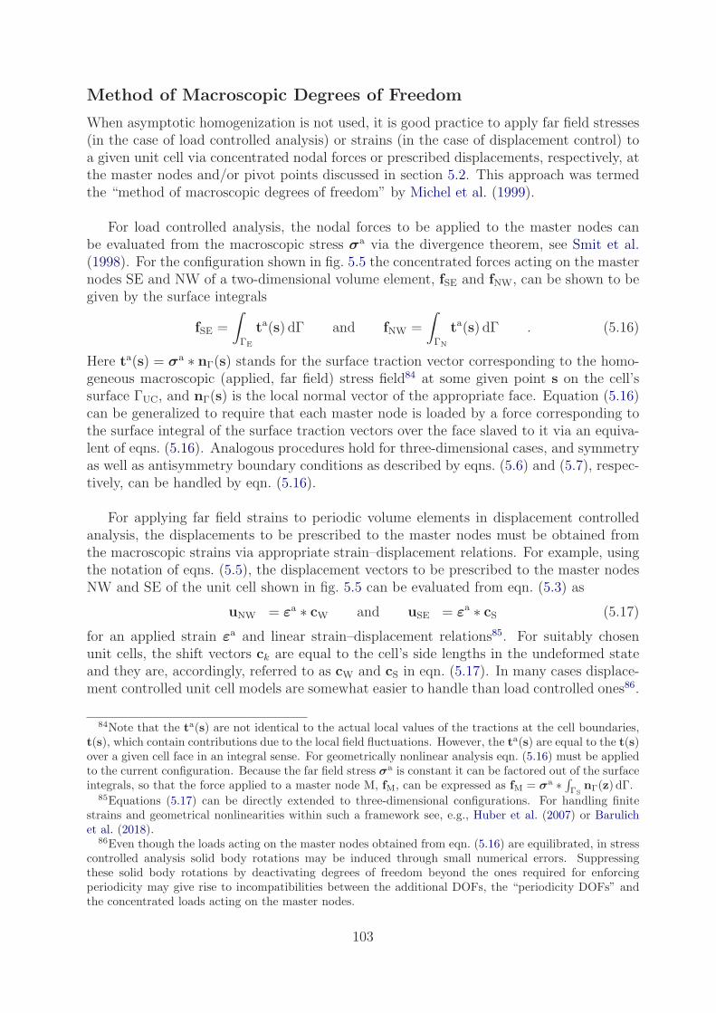
Method of Macroscopic Degrees of Freedom

When asymptotic homogenization is not used, it is good practice to apply far field stresses(in the case of load controlled analysis) or strains (in the case of displacement control) toa given unit cell via concentrated nodal forces or prescribed displacements, respectively, atthe master nodes and/or pivot points discussed in section 5.2. This approach was termedthe “method of macroscopic degrees of freedom” by Michel et al. (1999).

For load controlled analysis, the nodal forces to be applied to the master nodes canbe evaluated from the macroscopic stress σa via the divergence theorem, see Smit et al.(1998). For the configuration shown in fig. 5.5 the concentrated forces acting on the masternodes SE and NW of a two-dimensional volume element, fSE and fNW, can be shown to begiven by the surface integrals

fSE =

∫

ΓE

ta(s) dΓ and fNW =

∫

ΓN

ta(s) dΓ . (5.16)

Here ta(s) = σa ∗ nΓ(s) stands for the surface traction vector corresponding to the homo-geneous macroscopic (applied, far field) stress field84 at some given point s on the cell’ssurface ΓUC, and nΓ(s) is the local normal vector of the appropriate face. Equation (5.16)can be generalized to require that each master node is loaded by a force corresponding tothe surface integral of the surface traction vectors over the face slaved to it via an equiva-lent of eqns. (5.16). Analogous procedures hold for three-dimensional cases, and symmetryas well as antisymmetry boundary conditions as described by eqns. (5.6) and (5.7), respec-tively, can be handled by eqn. (5.16).

For applying far field strains to periodic volume elements in displacement controlledanalysis, the displacements to be prescribed to the master nodes must be obtained fromthe macroscopic strains via appropriate strain–displacement relations. For example, usingthe notation of eqns. (5.5), the displacement vectors to be prescribed to the master nodesNW and SE of the unit cell shown in fig. 5.5 can be evaluated from eqn. (5.3) as

uNW = εa ∗ cW and uSE = εa ∗ cS (5.17)

for an applied strain εa and linear strain–displacement relations85. For suitably chosenunit cells, the shift vectors ck are equal to the cell’s side lengths in the undeformed stateand they are, accordingly, referred to as cW and cS in eqn. (5.17). In many cases displace-ment controlled unit cell models are somewhat easier to handle than load controlled ones86.

84Note that the ta(s) are not identical to the actual local values of the tractions at the cell boundaries,t(s), which contain contributions due to the local field fluctuations. However, the ta(s) are equal to the t(s)over a given cell face in an integral sense. For geometrically nonlinear analysis eqn. (5.16) must be appliedto the current configuration. Because the far field stress σa is constant it can be factored out of the surfaceintegrals, so that the force applied to a master node M, fM, can be expressed as fM = σa ∗

∫ΓS

nΓ(z) dΓ.85Equations (5.17) can be directly extended to three-dimensional configurations. For handling finite

strains and geometrical nonlinearities within such a framework see, e.g., Huber et al. (2007) or Barulichet al. (2018).

86Even though the loads acting on the master nodes obtained from eqn. (5.16) are equilibrated, in stresscontrolled analysis solid body rotations may be induced through small numerical errors. Suppressingthese solid body rotations by deactivating degrees of freedom beyond the ones required for enforcingperiodicity may give rise to incompatibilities between the additional DOFs, the “periodicity DOFs” andthe concentrated loads acting on the master nodes.

103

In general, the overall stress and strain tensors within a unit cell can be evaluatedby volume averaging87 or by using the equivalent surface integrals given in eqn. (1.4). Inpractice, it is often fairly straightforward to approximate volume integrals by numericalintegration schemes such as eqns. (4.8) of (4.10), whereas comparably convenient approxi-mations are not available for surface integrals within an FE framework.

In the case of rectangular or hexahedral unit cells or reduced cells that are aligned withthe coordinate axes, averaged engineering stress and strain components can, of course,be evaluated by dividing the applied or reaction forces at the master nodes by the ap-propriate surface areas and by dividing the displacements of the master nodes by theappropriate cell lengths, respectively. The displacements of and concentrated forces actingon the master nodes can also be used for evaluating the macroscopic stresses and strainsfrom skewed unit cells having non-rectangular periodicity vectors, see, e.g., Pahr (2003),where also some additional aspects of unit cells, master nodes, and the method of macro-scopic degrees of freedom are discussed. Care is required in applying as well as evaluatingmacroscopic stresses and strains if the volume elements are not quadrilaterals or hexahedra.

In order to obtain three-dimensional homogenized elastic tensors with the method ofmacroscopic degrees of freedom six suitable, linearly independent load cases must be solvedfor in the most general case.

5.4 Periodic Models for Composites Reinforced by

Continuous Fibers

A wide range of periodic models have been reported for the most important groups ofcontinuously reinforced composites, viz., unidirectionally reinforced, angle-ply and cross-ply materials, as well as fabric reinforced composites.

Composites Reinforced by Unidirectional Continuous Fibers

Composites reinforced by continuous, aligned fibers typically show a statistically trans-versely isotropic overall behavior and can be studied well with periodic homogenization.Materials characterization with the exception of the overall axial shear behavior can becarried out with two-dimensional unit cell or reduced cell models employing generalizedplane strain elements that use a global degree of freedom for describing the axial defor-mation of the whole model88. For handling the overall axial shear response (required, e.g.,for establishing macroscopic elasticity tensors) special generalized plane strain elements(Adams and Crane, 1984; Sørensen, 1992) or three-dimensional models with appropriate

87For finite strain analysis the consistent procedure is to first average the deformation gradients andthen evaluate the strains from these averages.

88Generalized plane strain elements suitable for such analysis are implemented in a number of commercialFE codes. Because the axial stiffness of composites reinforced by continuous aligned fibers can usuallybe satisfactorily described by Voigt-type (“rule of mixture”) models, PMA studies of such materials havetended to concentrate on the transverse behavior. Note that plane strain models do not properly accountfor the axial constraints in such materials.

104

PH0CH1RH2CH3

PS0MS5CS7CS8

Figure 5.8: Eight simple periodic fiber arrangements of fiber volume fraction ξ=0.475 for modelingcontinuously fiber reinforced composites (Bohm and Rammerstorfer, 1995).

periodicity boundary conditions, see, e.g., Pettermann and Suresh (2000), are required89.Three-dimensional modeling is required for materials characterization of composites rein-forced by continuous aligned fibers when the effects of fiber misalignment, of fiber waviness(Garnich and Karami, 2004), of pores in the matrix, or of broken fibers90 (Mahishi, 1986)or of local damage to matrix or interface are to be studied. Unit cell models used for gen-eral nonlinear constitutive modeling of continuously reinforced composites must be fullythree-dimensional and employ periodicity boundary conditions.

The most basic generalized plane strain models of continuously reinforced compositesmake use of simple periodic fiber arrangements as shown in fig. 5.8, all of which canbe described by rather small reduced cells using symmetry and/or antisymmetry B.Cs,compare fig. 5.2. The simplest among these phase geometries are the periodic hexagonal(PH0) and periodic square (PS0) arrays, the use of which goes back to the 1960s (Adamsand Doner, 1967). Models with hexagonal symmetry (PH0,CH1,RH2,CH3) give rise totransversely isotropic thermoelastic overall behavior91 whereas the other fiber arrangementsshown in fig. 5.8 have tetragonal (PS0,CS7,CS8) or monoclinic (MS5) overall symmetry. Inthe elastoplastic and damage regimes the macroscopic symmetries of the fiber arrangementsare degraded for most load cases, compare fig. 5.9, and hexagonal arrangements are not

89For linear elastic material behavior there is the additional option of describing out-of-plane shearbehavior via the formal analogy between antiplane shear and diffusion (e.g., conduction) problems.

90For investigating the axial failure behavior of continuously reinforced MMCs, statistical methodsconcentrating on fiber fragmentation within spring lattice models, see, e.g., Zhou and Curtin (1995),have been used successfully.

91Like the macroscopic elastic responses, the phase averages of the local stress and strain fields ofhexagonal arrangements of aligned fibers are independent of the orientations of transverse loads. Thehigher statistical moments and the distributions function of these fields at the phase level, however, mayshow such a dependence. Consequently, the equivalent stress varies to some extent with the loadingdirection, which underlies the small differences in initial yielding between the two “PH” curves in fig. 5.9.

105

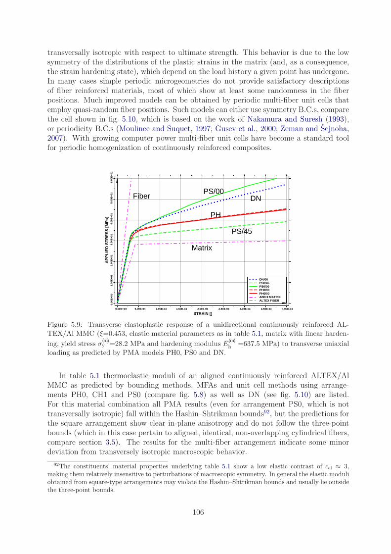
transversally isotropic with respect to ultimate strength. This behavior is due to the lowsymmetry of the distributions of the plastic strains in the matrix (and, as a consequence,the strain hardening state), which depend on the load history a given point has undergone.In many cases simple periodic microgeometries do not provide satisfactory descriptionsof fiber reinforced materials, most of which show at least some randomness in the fiberpositions. Much improved models can be obtained by periodic multi-fiber unit cells thatemploy quasi-random fiber positions. Such models can either use symmetry B.C.s, comparethe cell shown in fig. 5.10, which is based on the work of Nakamura and Suresh (1993),or periodicity B.C.s (Moulinec and Suquet, 1997; Gusev et al., 2000; Zeman and Sejnoha,2007). With growing computer power multi-fiber unit cells have become a standard toolfor periodic homogenization of continuously reinforced composites.

0.0

0E+0

0 1

.00E

+01

2.0

0E+0

1 3

.00E

+01

4.0

0E+0

1 5

.00E

+01

6.0

0E+0

1

AP

PL

IED

ST

RE

SS

[M

Pa]

0.00E+00 5.00E-04 1.00E-03 1.50E-03 2.00E-03 2.50E-03 3.00E-03 3.50E-03 4.00E-03

STRAIN []

ALTEX FIBERAl99.9 MATRIXPH0/00PH0/90PS0/00PS0/45DN/00

Fiber

Matrix

PS/45

PH

DNPS/00

Figure 5.9: Transverse elastoplastic response of a unidirectional continuously reinforced AL-TEX/Al MMC (ξ=0.453, elastic material parameters as in table 5.1, matrix with linear harden-

ing, yield stress σ(m)y =28.2 MPa and hardening modulus E

(m)h =637.5 MPa) to transverse uniaxial

loading as predicted by PMA models PH0, PS0 and DN.

In table 5.1 thermoelastic moduli of an aligned continuously reinforced ALTEX/AlMMC as predicted by bounding methods, MFAs and unit cell methods using arrange-ments PH0, CH1 and PS0 (compare fig. 5.8) as well as DN (see fig. 5.10) are listed.For this material combination all PMA results (even for arrangement PS0, which is nottransversally isotropic) fall within the Hashin–Shtrikman bounds92, but the predictions forthe square arrangement show clear in-plane anisotropy and do not follow the three-pointbounds (which in this case pertain to aligned, identical, non-overlapping cylindrical fibers,compare section 3.5). The results for the multi-fiber arrangement indicate some minordeviation from transversely isotropic macroscopic behavior.

92The constituents’ material properties underlying table 5.1 show a low elastic contrast of cel ≈ 3,making them relatively insensitive to perturbations of macroscopic symmetry. In general the elastic moduliobtained from square-type arrangements may violate the Hashin–Shtrikman bounds and usually lie outsidethe three-point bounds.

106

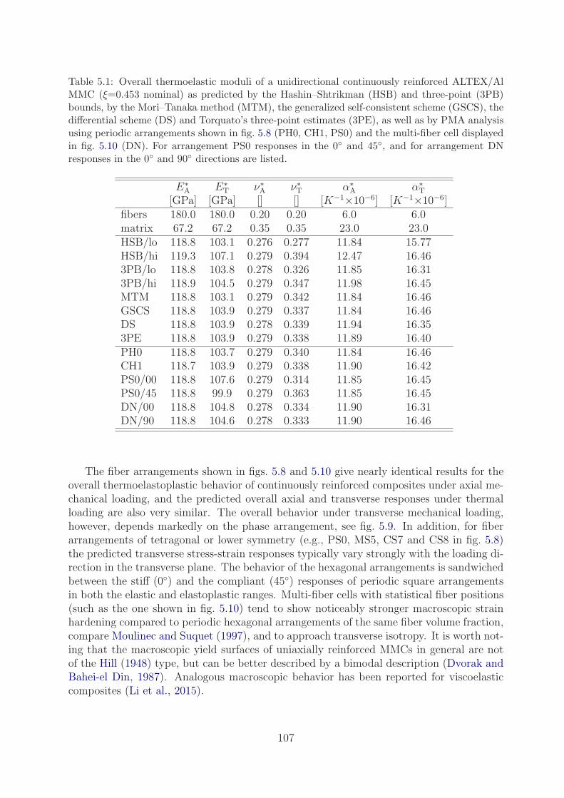
Table 5.1: Overall thermoelastic moduli of a unidirectional continuously reinforced ALTEX/AlMMC (ξ=0.453 nominal) as predicted by the Hashin–Shtrikman (HSB) and three-point (3PB)bounds, by the Mori–Tanaka method (MTM), the generalized self-consistent scheme (GSCS), thedifferential scheme (DS) and Torquato’s three-point estimates (3PE), as well as by PMA analysisusing periodic arrangements shown in fig. 5.8 (PH0, CH1, PS0) and the multi-fiber cell displayedin fig. 5.10 (DN). For arrangement PS0 responses in the 0 and 45, and for arrangement DNresponses in the 0 and 90 directions are listed.

E∗A E∗

T ν∗A ν∗T α∗A α∗

T

[GPa] [GPa] [] [] [K−1×10−6] [K−1×10−6]fibers 180.0 180.0 0.20 0.20 6.0 6.0matrix 67.2 67.2 0.35 0.35 23.0 23.0HSB/lo 118.8 103.1 0.276 0.277 11.84 15.77HSB/hi 119.3 107.1 0.279 0.394 12.47 16.463PB/lo 118.8 103.8 0.278 0.326 11.85 16.313PB/hi 118.9 104.5 0.279 0.347 11.98 16.45MTM 118.8 103.1 0.279 0.342 11.84 16.46GSCS 118.8 103.9 0.279 0.337 11.84 16.46DS 118.8 103.9 0.278 0.339 11.94 16.353PE 118.8 103.9 0.279 0.338 11.89 16.40PH0 118.8 103.7 0.279 0.340 11.84 16.46CH1 118.7 103.9 0.279 0.338 11.90 16.42PS0/00 118.8 107.6 0.279 0.314 11.85 16.45PS0/45 118.8 99.9 0.279 0.363 11.85 16.45DN/00 118.8 104.8 0.278 0.334 11.90 16.31DN/90 118.8 104.6 0.278 0.333 11.90 16.46

The fiber arrangements shown in figs. 5.8 and 5.10 give nearly identical results for theoverall thermoelastoplastic behavior of continuously reinforced composites under axial me-chanical loading, and the predicted overall axial and transverse responses under thermalloading are also very similar. The overall behavior under transverse mechanical loading,however, depends markedly on the phase arrangement, see fig. 5.9. In addition, for fiberarrangements of tetragonal or lower symmetry (e.g., PS0, MS5, CS7 and CS8 in fig. 5.8)the predicted transverse stress-strain responses typically vary strongly with the loading di-rection in the transverse plane. The behavior of the hexagonal arrangements is sandwichedbetween the stiff (0) and the compliant (45) responses of periodic square arrangementsin both the elastic and elastoplastic ranges. Multi-fiber cells with statistical fiber positions(such as the one shown in fig. 5.10) tend to show noticeably stronger macroscopic strainhardening compared to periodic hexagonal arrangements of the same fiber volume fraction,compare Moulinec and Suquet (1997), and to approach transverse isotropy. It is worth not-ing that the macroscopic yield surfaces of uniaxially reinforced MMCs in general are notof the Hill (1948) type, but can be better described by a bimodal description (Dvorak andBahei-el Din, 1987). Analogous macroscopic behavior has been reported for viscoelasticcomposites (Li et al., 2015).

107

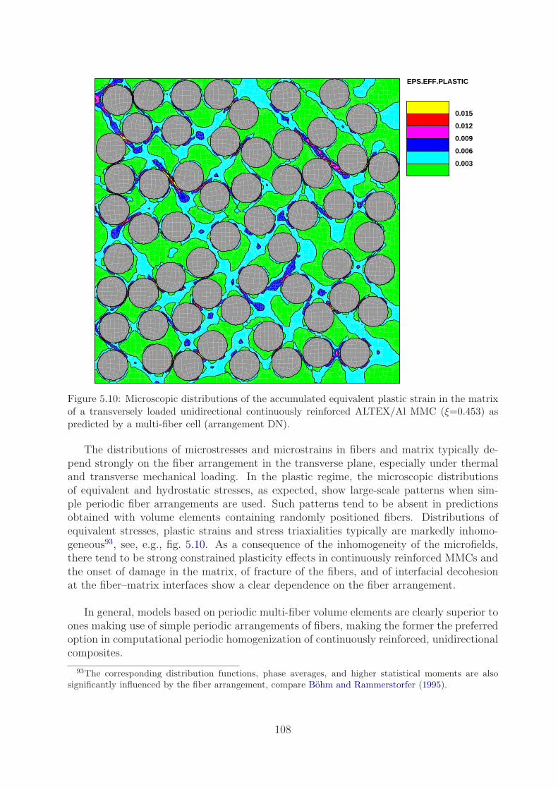
EPS.EFF.PLASTIC

0.015

0.012

0.009

0.006

0.003

Figure 5.10: Microscopic distributions of the accumulated equivalent plastic strain in the matrixof a transversely loaded unidirectional continuously reinforced ALTEX/Al MMC (ξ=0.453) aspredicted by a multi-fiber cell (arrangement DN).

The distributions of microstresses and microstrains in fibers and matrix typically de-pend strongly on the fiber arrangement in the transverse plane, especially under thermaland transverse mechanical loading. In the plastic regime, the microscopic distributionsof equivalent and hydrostatic stresses, as expected, show large-scale patterns when sim-ple periodic fiber arrangements are used. Such patterns tend to be absent in predictionsobtained with volume elements containing randomly positioned fibers. Distributions ofequivalent stresses, plastic strains and stress triaxialities typically are markedly inhomo-geneous93, see, e.g., fig. 5.10. As a consequence of the inhomogeneity of the microfields,there tend to be strong constrained plasticity effects in continuously reinforced MMCs andthe onset of damage in the matrix, of fracture of the fibers, and of interfacial decohesionat the fiber–matrix interfaces show a clear dependence on the fiber arrangement.

In general, models based on periodic multi-fiber volume elements are clearly superior toones making use of simple periodic arrangements of fibers, making the former the preferredoption in computational periodic homogenization of continuously reinforced, unidirectionalcomposites.

93The corresponding distribution functions, phase averages, and higher statistical moments are alsosignificantly influenced by the fiber arrangement, compare Bohm and Rammerstorfer (1995).

108

Cross-Ply and Angle-Ply Composites

Another group of composite materials reinforced by continuous fibers that can be studiedto advantage by unit cell methods are laminates consisting of plies the thickness of whichis not much greater than the fiber diameter. The left side of fig. 5.11 depicts a unit cell fora cross-ply laminate with double layers of fibers which is suitable for use with periodicityand symmetry boundary conditions. In the the center a minimum reduced cell for crossply laminates with one fiber layer per ply is shown, which requires the use of symmetryboundary conditions. A unit cell for studying angle-ply laminates with a general ply angleβ via periodicity boundary conditions is displayed on the right side of fig. 5.11. Extendingmodels of the above type to multi-fiber cells with randomly arranged fiber positions appearsfeasible.

β

oo90 plies

0 ply

Figure 5.11: Unit cell for a double layer cross-ply laminate (left), minimum reduced cell for across ply-laminate (center) and unit cell for an angle-ply laminate with ply angle β (right).

Unit cells with symmetry boundary conditions were used for studying the thermome-chanical behavior of cross ply laminates, e.g., by Lerch et al. (1991) as well as Ismar andSchroter (2000), and volume elements with periodicity BC, e.g., by Soni et al. (2014). Forunit cell studies of angle ply laminates see, e.g., Xia et al. (2003) and Abolfathi et al.(2008).

Fabric Reinforced Composites

Periodic homogenization has played an important role in modeling the behavior of fabricreinforced composites, i.e., materials containing woven, braided, or knitted reinforcements,see, e.g., Ivanov and Lomov (2020). In such “textile composites” the reinforcing phasetakes the form of textile-like structures consisting of interlacing bundles of continuousfibers (tows). Unit cell and reduced cell models for such materials are typically based onmodeling fiber bundles as a “mesophase” with smeared-out material properties, which, inturn, are obtained from analyzing unidirectionally continuously reinforced composites94.Free surface boundary conditions are specified for the out-of-plane faces of the cell, anda number of cells may be stacked on top of each other in order to account for in-planeoffsets and constraint effects between the layers (Bystrom et al., 2000). Symmetry bound-ary conditions can be specified for the in-plane faces, giving reasonably small unit cells as

94This modeling strategy obviously is a type of multiscale modeling as discussed in chapter 8.

109

shown in fig. 5.12, and combinations of periodicity, symmetry and antisymmetry bound-ary conditions may be used to achieve very small volume elements, see, e.g., (Tang andWhitcomb, 2003). Such models, however, are restricted to handling in-plane normal andthermal loads. By applying extended periodicity boundary conditions to larger unit cellsmacroscopic rotational degrees of freedom can be introduced to allow studying all defor-mation modes, including the macroscopic warping and twisting of the laminae.

TowsCompositeMatrix

Figure 5.12: Schematic of a reduced cell using symmetry boundary conditions for modeling aplain weave lamina. The tow region (left), the matrix region (center) and the “assembled” unitcell (right) are shown.

There is a wide range of weaves as well as knitting and braiding architectures that canbe modeled with PMAs. Unit cells for woven, knitted and braided composites tend to befairly complex geometrically, may be difficult to mesh for Finite Element analysis and maypose considerable computational requirements, especially when nonlinear behavior is tobe studied. Over the past 25 years a considerable number of studies have been publishedon unit cell modeling of fabric reinforced composites, see, e.g., Cox and Flanagan (1997),Huang and Ramakrishna (2000), Tang and Whitcomb (2003) or Lomov et al. (2006), andon software for generating appropriate unit cells (Robitaille et al., 2003; Sherburn, 2007).Gager and Pettermann (2012) proposed shell element-based unit cells for textile compos-ites that can significantly reduce the modeling effort.

5.5 Periodic Models for Composites Reinforced by

Short Fibers

The overall symmetry of short fiber reinforced composites in many cases is isotropic (forrandom fiber orientations) or transversely isotropic (for aligned fibers, planar random fibersand other fiber arrangements with axisymmetric orientation distributions). However, pro-cessing conditions can give rise to a wide range of fiber orientation distributions and,consequently, lower overall symmetries (Allen and Lee, 1990). The thermoelastic and ther-moelastoplastic behavior of aligned short fiber reinforced composites has been successfully

110

estimated by Mori–Tanaka methods95, which can also be extended to nonaligned fibers andreinforcements showing an aspect ratio distribution, compare section 2.6. Such mean-fieldapproaches are, however, limited in resolving details of fiber arrangements, especially forinelastic material behavior. At present the most powerful tools for studying the influenceof fiber shapes and orientations, of clustering effects, of the interaction of fibers of dif-ferent sizes, and of local stress and strain fields between neighboring fibers are periodicmicrofield methods. Platelet reinforced composites can be described by analogy to shortfiber reinforced materials.

Composites Reinforced by Aligned Short Fibers

In contrast to continuously reinforced composites, the phase arrangements of discontinu-ously reinforced materials are inherently three-dimensional. The simplest three-dimensionalPMA models of aligned short fiber reinforced composites have used periodic square ar-rangements of non-staggered or staggered aligned cylindrical fibers96 see, e.g., Levy andPapazian (1991) and compare fig. 5.13. Such geometries are relatively simple to set upand do not pose major computational requirements, but are rather restrictive in terms

Figure 5.13: Three-dimensional cells for modeling non-staggered (left) and staggered (right)square arrangements of aligned short fibers. The shaded reduced cells, which follow Levy andPapazian (1991), require symmetry B.C., cells outlined in bold are suitable for periodicity B.C.

95For a comparison between unit cell and analytical predictions for the overall elastic properties of shortfiber reinforced composites see, e.g., Tucker and Liang (1999).

96Such square arrangements give rise to tetragonal overall symmetry, and, consequently, the transverseoverall properties are direction dependent.

111

of fiber arrangements and load conditions that can be handled. By using larger volumeelements supporting periodicity boundary conditions the full thermomechanical behaviorof the fiber arrangements can be studied. Analogous microgeometries based on periodichexagonal arrangements of non-staggered (Jarvstrat, 1992) or staggered (Tucker and Liang,1999) fibers as well as ellipsoidal cells aimed at describing composite “ellipsoid assembly”microgeometries (Jarvstrat, 1993) were also proposed.

For many materials characterization studies, a more economical alternative to the abovethree-dimensional unit cells takes the form of axisymmetric models describing the axialbehavior of non-staggered or staggered arrays of aligned cylindrical short fibers in an ap-proximate way. The basic idea behind these models is replacing unit cells for square orhexagonal arrangements by circular composite cylinders of equivalent cross sectional area(and volume fraction) as sketched in Fig. 5.14. The resulting axisymmetric cells are notproper unit cells, because they overlap and are not space filling. In addition, their as-sociation with three-dimensional phase arrangements is somewhat tenuous — note thatthey do not show the same transverse fiber spacing as the “equivalent” periodic arrange-ments in Fig. 5.14 — and they are severely limited in the type of loading conditions theycan handle97. However, they have the advantage of significantly reduced computationalrequirements, which has made them especially suitable for qualitative studies of highlynonlinear behavior such as damage.

Figure 5.14: Periodic arrays of aligned non-staggered (top) and staggered (bottom) short fibersand corresponding axisymmetric cells (left: sections in transverse plane; right: sections parallelto fibers).

97Axisymmetric cells are limited to load cases in which the deformed shape of the cell remains axisym-metric. These include uniaxial stress and strain, volumetric stress, “in plane hydrostatic stress” (wherea homogeneous radial stress is prescribed) and isochoric strain (obtained, in the small strain regime, byapplying constant normal displacements at the “upper” and “outer” faces of, vN = 2uE , respectively).

112

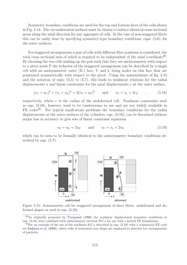
Symmetry boundary conditions are used for the top and bottom faces of the cells shownin Fig. 5.14. The circumferential surfaces must be chosen to enforce identical cross sectionalareas along the axial direction for any aggregate of cells. In the case of non-staggered fibersthis can be easily done by specifying symmetry-type boundary conditions, eqns. (5.6), forthe outer surfaces.

For staggered arrangements a pair of cells with different fiber positions is considered, thetotal cross sectional area of which is required to be independent of the axial coordinate98.By choosing the two cells making up the pair such that they are antisymmetric with respectto a pivot point P the behavior of the staggered arrangement can be described by a singlecell with an antisymmetric outer (E-) face, U and L being nodes on this face that arepositioned symmetrically with respect to the pivot. Using the nomenclature of fig. 5.15and the notation of eqns. (5.5) to (5.7), this leads to nonlinear relations for the radialdisplacements u and linear constraints for the axial displacements v at the outer surface,

(rU + uU)2 + (rL + uL)2 = 2(rP + uP)2 and vU + vL = 2vP , (5.18)

respectively, where r is the radius of the undeformed cell. Nonlinear constraints suchas eqn. (5.18), however, tend to be cumbersome to use and are not widely available inFE codes99. For typical small-strain problems the boundary conditions for the radialdisplacements at the outer surfaces of the cylinders, eqn. (5.18), can be linearized withoutmajor loss in accuracy to give sets of linear constraint equations

uU + uL = 2uP and vU + vL = 2vP , (5.19)

which can be seen to be formally identical to the antisymmetry boundary conditions de-scribed by eqn. (5.7).

NW

SE

NE

NW

NE

SE

W

S

N

W

N

E

S

E

s

−s

undeformed deformed

L

UU

P

L

r

z

r

zP

~

~SW SW

Figure 5.15: Axisymmetric cell for staggered arrangement of short fibers: undeformed and de-formed shapes as used in eqn. (5.18).

98As originally proposed by Tvergaard (1990) the nonlinear displacement boundary conditions ineqn. (5.18) were combined with antisymmetry traction B.C.s for use with a hybrid FE formulation.

99For an example of the use of the nonlinear B.C.s described in eqn. (5.18) with a commercial FE codesee Ishikawa et al. (2000), where cells of truncated cone shape are employed to describe bcc arrangementsof particles.

113

Axisymmetric cell models of the types shown in fig. 5.14 were the the workhorses ofPMA studies of short fiber reinforced composites in the 1990s, see, e.g., Povirk et al. (1992)or Tvergaard (1994). Typically, descriptions using staggered arrangements allow a widerrange of microgeometries to be covered, compare Bohm et al. (1993) or Tvergaard (2003),and give more realistic descriptions of actual composites. Both staggered and non-staggeredaxisymmetric models can be extended to studying a considerable range of arrangementsincorporating aligned fibers of different size and/or aspect ratio by coupling two or moredifferent cells via the condition of keeping the cross sectional area of the aggregate inde-pendent of the axial coordinate (Bohm et al., 1993).

Axisymmetric cells and simple three-dimensional unit cells have been used successfullyfor studying the nonlinear thermomechanical behavior of aligned short fiber reinforcedMMCs, e.g., with respect to the their stress–strain responses, to the pseudo-Bauschingereffect, and to thermal residual stresses. They have provided valuable insight into causesand effects of matrix, interface and fiber damage. Over the past years, however, multi-fiber unit cells have become the standard tool for studying composites reinforced by alignedshort fibers.

Composites Reinforced by Nonaligned Short Fibers

Among the first unit cell studies of materials reinforced by nonaligned discontinuous fiberswere based on three-dimensional models of composites reinforced by alternatingly tiltedmisaligned fibers (Sørensen et al., 1995) and plane-stress models describing planar randomshort fibers (Courage and Schreurs, 1992). Multi-fiber unit cells of such materials havestarted coming into their own in the 2000s. It is worth noting that the situation with re-spect to mean-field models for composites reinforced by short fibers is not fully satisfactoryfor the elastic range, compare section 2.6, and MFAs have found limited application forwork on inelastic thermomechanical behavior.

At present the most powerful continuum modeling strategy for nonaligned short fiberreinforced composites consists of using three-dimensional multi-fiber volume elements inwhich the fibers are randomly positioned and oriented such that the required ODF is ful-filled to a suitable level of approximation. If the geometries are periodic, they are obviouslysuitable for periodic homogenization. Among early reports for such multi-fiber unit cellswere, e.g., Lusti et al. (2002) or Bohm et al. (2002) for spatially random fiber orientationsand Duschlbauer et al. (2006) or Iorga et al. (2008) for planar random fiber orientations.Models of this type can also account for the distributions of fiber sizes and/or aspect ratios.Such modeling approaches tend to pose considerable challenges in generating appropriatefiber arrangements at non-dilute volume fractions due to geometrical frustration, relativelylarge volume elements being required for handling periodic microgeometries with fiber as-pect ratio in excess of, say, 5. The meshing of the resulting phase arrangements for usewith the FEM may also be difficult, compare Shephard et al. (1995), and analyzing themechanical response of the resulting cells may require considerable computing power, es-pecially for nonlinear constituent behavior. The first studies of this type were, accordingly,restricted to the linear elastic range, where the BEM has been found to answer well, see,e.g., Banerjee and Henry (1992). Commercial micromechanics codes such as Digimat (e-Xstream Engineering, Mont-Saint-Guibert, Belgium) have become available that provide

114

capabilities for setting up and solving periodic models with considerable numbers of non-aligned short fibers.

As a simple example of a multi-fiber unit cell for a composite reinforced by nonalignedshort fibers, fig. 5.16 shows a cube-shaped cell that contains 15 randomly oriented cylindri-cal fibers of aspect ratio a = 5, supports periodicity boundary conditions, was generatedby random sequential addition, and is discretized by tetrahedral elements. The phase ar-rangement is set up in such a way that spheroidal fibers of the same aspect ratio, volumefractions, center points, and orientations can also be used in order to allow studying fibershape effects (Bohm et al., 2002).

Figure 5.16: Unit cell for a composite reinforced by randomly oriented short fibers (Bohm et al.,2002). The nominal fiber volume fraction is ξ = 0.15 and the 15 cylindrical fibers in the cell havean aspect ratio of a = 5.

Table 5.2 lists predictions for the overall elastic response of a composite reinforcedby randomly positioned and oriented fibers obtained by analytical estimates, the Hashin–Shtrikman bounds (Hashin and Shtrikman, 1963) and results obtained with the abovetype of unit cell, for which data are shown pertaining to cylindrical and spheroidal fibers.Interestingly, noticeable differences were found between the predictions for reinforcementby cylindrical and spheroidal fibers that have the same fiber volume fraction and aspectratio, occupy the same positions and show the same orientations, with the spheroidal rein-forcements leading to a more compliant response, especially in the inelastic regime. Usefulresults were obtained despite the low number of fibers in the unit cell and excellent agree-ment with analytical descriptions was achieved in terms of the orientation dependence ofthe stresses in individual fibers, compare fig. 2.4. Whereas the phase arrangement shownin fig. 5.16 does not contain a sufficient number of fibers for approaching representativenesseven in the elastic range, recent studies using much larger volume elements have markedlyimproved this situation, see, e.g., Tian et al. (2015).

115

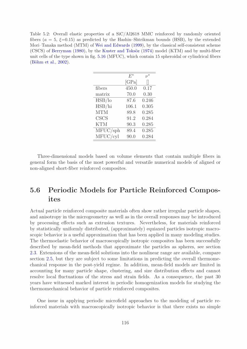
Table 5.2: Overall elastic properties of a SiC/Al2618 MMC reinforced by randomly orientedfibers (a = 5, ξ=0.15) as predicted by the Hashin–Shtrikman bounds (HSB), by the extendedMori–Tanaka method (MTM) of Wei and Edwards (1999), by the classical self-consistent scheme(CSCS) of Berryman (1980), by the Kuster and Toksoz (1974) model (KTM) and by multi-fiberunit cells of the type shown in fig. 5.16 (MFUC), which contain 15 spheroidal or cylindrical fibers(Bohm et al., 2002).

E∗ ν∗

[GPa] []fibers 450.0 0.17matrix 70.0 0.30HSB/lo 87.6 0.246HSB/hi 106.1 0.305MTM 89.8 0.285CSCS 91.2 0.284KTM 90.3 0.285MFUC/sph 89.4 0.285MFUC/cyl 90.0 0.284

Three-dimensional models based on volume elements that contain multiple fibers ingeneral form the basis of the most powerful and versatile numerical models of aligned ornon-aligned short-fiber reinforced composites.

5.6 Periodic Models for Particle Reinforced Compos-

ites

Actual particle reinforced composite materials often show rather irregular particle shapes,and anisotropy in the microgeometry as well as in the overall responses may be introducedby processing effects such as extrusion textures. Nevertheless, for materials reinforcedby statistically uniformly distributed, (approximately) equiaxed particles isotropic macro-scopic behavior is a useful approximation that has been applied in many modeling studies.The thermoelastic behavior of macroscopically isotropic composites has been successfullydescribed by mean-field methods that approximate the particles as spheres, see section2.3. Extensions of the mean-field solutions into the nonlinear range are available, comparesection 2.5, but they are subject to some limitations in predicting the overall thermome-chanical response in the post-yield regime. In addition, mean-field models are limited inaccounting for many particle shape, clustering, and size distribution effects and cannotresolve local fluctuations of the stress and strain fields. As a consequence, the past 30years have witnessed marked interest in periodic homogenization models for studying thethermomechanical behavior of particle reinforced composites.

One issue in applying periodic microfield approaches to the modeling of particle re-inforced materials with macroscopically isotropic behavior is that there exists no simple

116

periodic three-dimensional phase arrangement that shows matrix–inclusion topology andis inherently elastically isotropic100. Together with the wide variation in microgeome-tries and particle shapes in actual materials, this gives rise to nontrivial tradeoffs betweenkeeping computational requirements reasonably low (favoring simple particle shapes andtwo-dimensional or simple three-dimensional microgeometries) and obtaining sufficientlyrealistic models for a given purpose (best fulfilled by three-dimensional volume elementscontaining considerable numbers of randomly positioned particles of complex shape). Inmany respects periodic models of particle reinforced composites are subject to similar con-straints and use analogous approaches as work on short fiber reinforced composites.

Many three-dimensional unit cell studies of generic microgeometries for particle rein-forced composites have been based on simple cubic (sc), face centered cubic (fcc) or bodycentered cubic (bcc) arrays of spherical, cylindrical or cube-shaped particles, compare, e.g.,Hom and McMeeking (1991). By invoking the symmetries of these arrays and using sym-metry as well as antisymmetry boundary conditions, rather small “reduced” cells can beobtained for materials characterization101, compare Weissenbek et al. (1994) and fig. 5.17.In addition, work employing hexagonal or tetrakaidecahedral arrays of particles (Rodin,1993) and Voronoi cells for cubic arrays of particles (Li and Wongsto, 2004) was reported.

Figure 5.17: Examples of reduced cells for particle reinforced composites using cubic arrays ofinhomogeneities: s.c. arrangement of cubes, b.c.c. arrangement of cylinders and f.c.c. arrangementof spheres (Weissenbek et al., 1994).

The effective elastic tensors obtained from cubic arrays of particles show cubic symme-try102. As a consequence, the corresponding moduli do not necessarily fulfill the Hashin–Shtrikman bounds for macroscopically isotropic materials, and often lie outside the three-point bounds, compare table 5.3. Among the cubic arrays of particles, sc ones are easiest

100Even though volume elements in the shape of pentagonal dodecahedra and icosahedra have the ap-propriate symmetry properties (Christensen, 1987), they are not space filling.101Among the reduced cells shown in fig. 5.17 the one on the left uses symmetry boundary conditions and

is restricted in the load cases that can be handled. The other two cells employ antisymmetry B.C.s andcan be used more freely. Unit cells suitable for periodicity boundary conditions are considerably larger,but allow unrestricted modeling of the full thermomechanical response of cubic phase arrangements.102Cubic elastic symmetry is a special case of orthotropy with equal responses in all principal directions.

It gives rise to direction dependent moduli and requires three independent parameters for describing theelastic behavior. For a discussion of the elastic anisotropy of cubic materials see, e.g., Cazzani and Rovati(2003). The conduction and diffusion behavior of materials with cubic symmetry is isotropic.

117

to handle by unit cell models, but their mechanical behavior shows a more pronouncedanisotropy than do bcc and fcc arrangements.

Axisymmetric cells describing staggered or non-staggered arrangements of particles canbe used for materials characterization of particle reinforced composites in full analogy withshort fiber reinforced materials, compare figs. 5.14 and 5.15. By appropriate choice of thedimensions of the axisymmetric cells sc, bcc and fcc arrays of particles can be approximatedto some extent, and a range of axisymmetric particle shapes can be studied. Such modelswere a mainstay of PMA modeling of materials containing particulate inhomogeneities,see, e.g., Bao et al. (1991) or LLorca (1996). A related type of model are spherical cells(Guild and Kinloch, 1995).

Due to their low computational requirements and the relative ease of incorporatingirregular particle shapes, planar unit cell models of particle reinforced materials have alsobeen used to a considerable extent. Typically, plane stress models (which actually describethin “reinforced sheets” or the stress states at the surface of inhomogeneous bodies) showa more compliant and plane strain models (which describe reinforcing by aligned continu-ous fibers rather than by particles) show a stiffer overall response than three-dimensionaldescriptions, compare table 5.3. With respect to the overall behavior, plane stress analy-sis may be preferable to plane strain analysis, compare (Weissenbek, 1994), but no two-dimensional model gives satisfactory results in terms of the predicted microstress andmicrostrain distributions103 (Bohm and Han, 2001). Axisymmetric cell models typicallyprovide better results for the behavior of particle reinforced composites than do planar ones.

During the past 20 years studies based on increasingly complex three-dimensional phasearrangements have assumed a prominent role in the literature. Gusev (1997) used FiniteElement methods in combination with unit cells containing up to 64 statistically posi-tioned particles to describe the overall behavior of elastic particle reinforced composites.Hexahedral unit cells containing up to 10 particles in a perturbed cubic configuration(Watt et al., 1996) as well as cube shaped cells incorporating at least 15 spherical parti-cles in quasi-random arrangements (Bohm et al., 1999; Bohm and Han, 2001), comparefig. 5.18, or clusters of particles (Segurado et al., 2003; Lee et al., 2011b) were used inFinite Element based studies of elastoplastic particle reinforced MMCs and related materi-als. Three-dimensional simulations involving high numbers of particles have been reported,e.g., for investigating the elastic behavior of composites (Michel et al., 1999), for studyingbrittle matrix composites that develop damage (Zohdi and Wriggers, 2001), and for rubberreinforced polymers (Fond et al., 2001).

103One issue giving rise to difficulties in describing macroscopically isotropic phase arrangements withtwo-dimensional models is the latters’ lack of a proper hydrostatic load case. Its closest planar equivalent,equi-biaxial loading, is controlled by the plane strain bulk modulus, KT, or the plane stress bulk modulus,respectively, both of which differ from the “three-dimensional” bulk modulus K.In plastic regimes, plane stress configurations tend to give much higher equivalent plastic strains in thematrix and weaker overall hardening than do plane strain and generalized plane strain models using thesame planar phase geometry. The configurations of regions of concentrated strains that underlie thisbehavior depend strongly on the geometrical constraints, compare, e.g., Iung and Grange (1995), Ganseret al. (1998), Bohm et al. (1999) or Shen and Lissenden (2002). For continuously reinforced compositesunder transverse loading the equivalent plastic strains tend to concentrate in bands oriented at 45 to theloading directions, whereas the patterns are qualitatively different in particle reinforced materials.

118

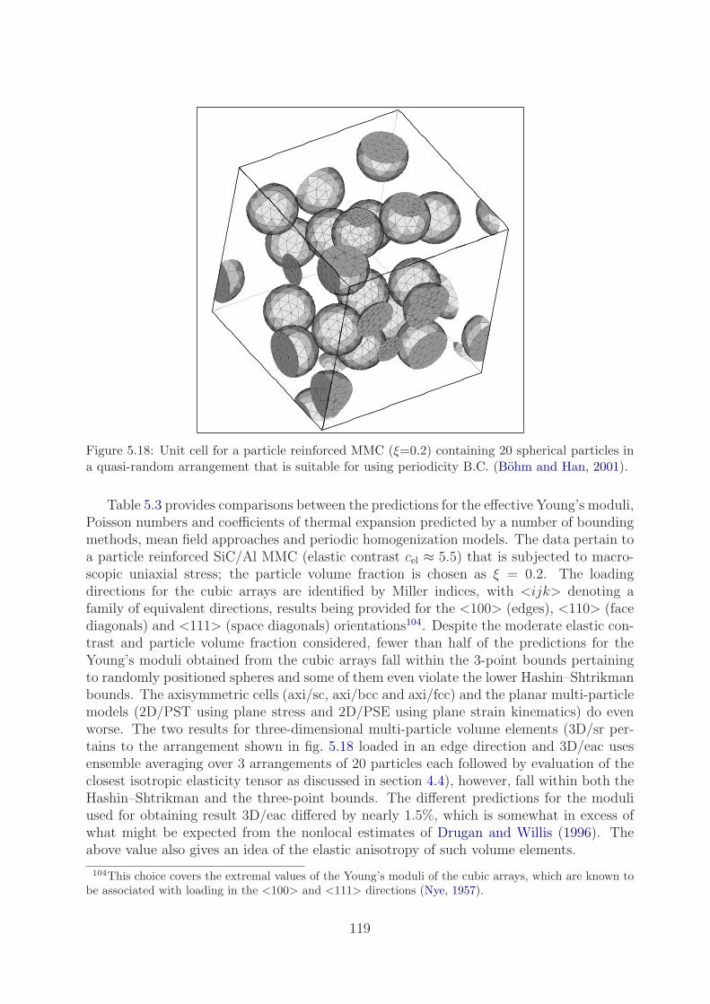
Figure 5.18: Unit cell for a particle reinforced MMC (ξ=0.2) containing 20 spherical particles ina quasi-random arrangement that is suitable for using periodicity B.C. (Bohm and Han, 2001).

Table 5.3 provides comparisons between the predictions for the effective Young’s moduli,Poisson numbers and coefficients of thermal expansion predicted by a number of boundingmethods, mean field approaches and periodic homogenization models. The data pertain toa particle reinforced SiC/Al MMC (elastic contrast cel ≈ 5.5) that is subjected to macro-scopic uniaxial stress; the particle volume fraction is chosen as ξ = 0.2. The loadingdirections for the cubic arrays are identified by Miller indices, with <ijk> denoting afamily of equivalent directions, results being provided for the <100> (edges), <110> (facediagonals) and <111> (space diagonals) orientations104. Despite the moderate elastic con-trast and particle volume fraction considered, fewer than half of the predictions for theYoung’s moduli obtained from the cubic arrays fall within the 3-point bounds pertainingto randomly positioned spheres and some of them even violate the lower Hashin–Shtrikmanbounds. The axisymmetric cells (axi/sc, axi/bcc and axi/fcc) and the planar multi-particlemodels (2D/PST using plane stress and 2D/PSE using plane strain kinematics) do evenworse. The two results for three-dimensional multi-particle volume elements (3D/sr per-tains to the arrangement shown in fig. 5.18 loaded in an edge direction and 3D/eac usesensemble averaging over 3 arrangements of 20 particles each followed by evaluation of theclosest isotropic elasticity tensor as discussed in section 4.4), however, fall within both theHashin–Shtrikman and the three-point bounds. The different predictions for the moduliused for obtaining result 3D/eac differed by nearly 1.5%, which is somewhat in excess ofwhat might be expected from the nonlocal estimates of Drugan and Willis (1996). Theabove value also gives an idea of the elastic anisotropy of such volume elements.

104This choice covers the extremal values of the Young’s moduli of the cubic arrays, which are known tobe associated with loading in the <100> and <111> directions (Nye, 1957).

119

Table 5.3: Overall thermoelastic properties of a particle reinforced SiC/Al MMC (spherical par-ticles, ξ=0.2) predicted by the Hashin–Shtrikman (HSB) and three-point (3PB) bounds, by theMori–Tanaka method (MTM), the generalized self-consistent scheme (GSCS), the differentialscheme (DS), and Torquato’s three-point estimates (3PE), as well as by unit cell analysis usingthree-dimensional cubic arrays, axisymmetric cells approximating sc, bcc and fcc geometries, two-dimensional multi-particle models based on plane stress (2D/PST) and plane strain (2D/PSE)kinematics, as well as three-dimensional models containing 20 randomly positioned spherical par-ticles (3D/sr and 3D/eac).

E∗ E∗<100> E∗<110> E∗<111> ν∗ α∗A

[GPa] [GPa] [GPa] [GPa] [] [K−1×10−6]particles 429.0 — — — 0.17 4.3matrix 67.2 — — — 0.35 23.0HSB/lo 91.2 — — — 0.285 16.8HSB/hi 115.4 — — — 0.340 18.53PB/lo 91.7 — — — 0.323 18.43PB/hi 94.2 — — — 0.328 18.5MTM 91.2 — — — 0.328 18.5GSCS 91.9 — — — 0.327 18.5DS 92.7 — — — 0.326 18.43PE 92.2 — — — 0.327 18.5sc — 96.5 90.6 89.5 18.5bcc — 90.1 91.8 92.2 18.5fcc — 90.2 91.7 92.1 18.5axi/sc 95.4 — — — 18.6/18.6axi/bcc 87.9 — — — / 18.4/18.8axi/fcc 88.1 — — — 18.1/19.02D/PST 85.5 — — — 0.3342D/PSE 98.7 — — —3D/sr 92.4 — — — 0.3263D/eac 92.2 — — — 0.327 18.5

The nonlinear macroscopic mechanical responses of particle reinforced composites tendto be more sensitive to the phase arrangements than is their elastic behavior. This isdemonstrated in fig. 5.19 where unit cell predictions for the macroscopic uniaxial tensileelastoplastic stress–strain responses of the same Al matrix as used in fig. 5.9 (von Misesplasticity with linear hardening), reinforced by 40 vol.% of spherical, linear elastic SiCparticles (identical to the ones in table 5.3), are compared. For the sc, bcc and fcc cubicarrays the responses to tensile loads acting in the <100>, <110> and <111> each areshown together with the ensemble averaged predictions for loads in the 3 edge directions oftwo volume elements containing 20 randomly positioned particles each, 3D/ea. Somewhatsimilarly to the case of fiber reinforced composites, fig. 5.9, the macroscopic hardeningbehavior of the multi-particle models is considerably more pronounced than that of thecubic arrays in most situations, then main exception being the sc array subjected to tensileuniaxial loading in <100>, which is excessively stiff.

120

0

1x107

2x107

3x107

4x107

5x107

6x107

7x107

0 0.001 0.002 0.003 0.004 0.005 0.006

APP

LIE

D S

TR

ESS

[M

Pa]

STRAIN []

sc, <100>sc, <110>sc, <111>

bcc, <100>bcc, <110>bcc, <111>fcc, <100>fcc, <110>fcc, <111>

MP/eavmatrix

Figure 5.19: Elastoplastic response of a particle reinforced SiC/Al MMC (ξ=0.4, matrix as infig. 5.9, particles as in table 5.3) to uniaxial loading as predicted by PMA models using sc, bccand fcc arrays as well as multi-particle volume elements (MP/eav).

Like fiber reinforced MMCs, particle reinforced composites typically display highly in-homogeneous microscopic stress and strain distributions, especially in nonlinear regimes.As an example, fig. 5.20, shows the predicted equivalent plastic strains of the elastoplasticmatrix inside the multi-particle unit cell model depicted in fig. 5.18. This behavior tends

SECTION FRINGE PLOTEPS.EFF.PLASTIC INC.12

5.0000E-02

4.0000E-02

3.0000E-02

2.0000E-02

1.0000E-02

SCALAR MIN: 6.6202E-04SCALAR MAX: 8.1576E-02

Figure 5.20: Predicted distribution of equivalent plastic strain in the matrix of a particle reinforcedMMC (ξ=0.2) subjected to uniaxial tensile loading (in left–right direction) obtained for a unitcell with 20 spherical particles in a quasi-random arrangement (Bohm and Han, 2001).

121

to give rise to microscopic “structures” that can be considerably larger than individualparticles, leading to longer ranged interactions between inhomogeneities105. The latter, inturn, underlie the need for larger volume elements for studying composites with nonlinearmatrix behavior mentioned in chapter 4.

Periodic volume elements are highly suitable for carrying out numerical experimentsthat explore the influence of different aspects of the microgeometry of particle reinforcedcomposites on their microscopic and macroscopic responses. For example, Rasool andBohm (2012) and Bohm and Rasool (2016) studied model composites that contain equalvolume fractions of randomly positioned and, where applicable, randomly oriented, identi-cal particles having the shapes of spheres, cubes, regular octahedra and regular tetrahedra,respectively. Figure 5.21 shows the resulting predictions for the responses to a single, non-symmetric, uniaxial stress loading cycle, clear effects of the particle shape on the hardeningbehavior and on the residual strains being evident.

-2.5

-2

-1.5

-1

-0.5

0

0.5

1

1.5

-0.005 0 0.005 0.01 0.015

NO

RM

AL

IZE

D M

AC

RO

SCO

PIC

ST

RE

SS [

]

MACROSCOPIC STRAIN []

SPHOCTCUBTET

Figure 5.21: PMA predictions for the responses to a uniaxial load cycle of elastoplastic, particlereinforced MMCs (ξ=0.2) containing identical spherical (SPH), cube-shaped (CUB), octahedral(OCT) and tetrahedral (TET) inhomogeneities, respectively.

A comparison of the modeling approaches for studying the mechanical behavior of par-ticle reinforced composites discussed in this section clearly brings out three-dimensionalmulti-particle models as being superior to the other options for evaluating both macro-scopic responses and microscopic stress and strain fields. Their main drawback, however,are their computational costs, especially for nonlinear problems.

105Due to the filtering effect of periodic phase arrangements mentioned in section 5.1, the length of suchfeatures can exceed the side length of the unit cell only in certain directions, which may induce a spuriousdirection dependence into the predicted large-strain behavior of sub-RVE unit cells. Cubic arrays giverise to highly regular, long range patterns of the microfields that may strongly favor such structures; themaxima of microfields in cubic arrays depend on the loading direction both in their location and magnitude.

122

5.7 Periodic Models for Porous and Cellular Materi-

als

Due to their relevance to the ductile damage and failure of metallic materials elastoplas-tic porous materials have been the subjects of a considerable number of PMA studies106.Generally, modeling concepts for porous materials are closely related to the ones employedfor particle reinforced composites, the main difference being that the shapes of the voidsmay evolve significantly through the loading history107. Axisymmetric cells of the typesdiscussed in sections 5.5 and 5.6, compare, e.g., Koplik and Needleman (1988) or Garajeuet al. (2000), and three-dimensional unit cells based on cubic arrangements of voids, see,e.g., McMeeking and Hom (1990) or Segurado et al. (2002b), have been used in the ma-jority of pertinent PMA studies. In addition, studies of void growth in ductile materialsbased on multi-void cells and using geometry data from serial sectioning were reported(Shan and Gokhale, 2001).

In cellular materials, such as foams, wood and trabecular bone, the volume fraction ofthe solid phase is very low (often amounting to no more than a few percent) and the voidphase may be topologically connected (open cell foams), unconnected (closed cell foams,syntactic foams), or both of the above (e.g., hollow sphere foams). The linear elastic regimeof cellular materials in many cases is limited to a very small range of macroscopic strains.Furthermore, marked differences tend to be present between tensile and compressive inelas-tic macroscopic responses: As strains increase, gross shape changes of the cells typicallytake place on the microscale, with large bending deformations, the formation of plastichinges, elastic as well as plastic buckling, and brittle failure of struts and cells walls play-ing major roles, especially under compressive loading. For compression-dominated loadcases this regime tends to give rise to a stress plateau on the macroscale, which underliesthe favorable energy absorption properties of many cellular materials. At some elevatedstrain the effective stiffness under compression typically rises sharply, the cellular structurehaving collapsed to such an extent that many cell walls or struts are in contact and thevoid volume fraction has decreased dramatically. No comparable behavior is present undertensile or shear loading.

Periodic microfield methods are generally well suited to studying the thermomechanicalbehavior of cellular materials. The widely used analytical results of Gibson and Ashby(1988) were derived by analytically studying arrangements of beams (for open cell foams)

106Many models and constitutive descriptions of the ductile damage and failure of metals, among themcontributions by Rice and Tracey (1969), Gurson (1977), Tvergaard and Needleman (1984), Gologanuet al. (1997) as well as Benzerga and Besson (2001), are based on micromechanics-based considerations ofthe growth of pre-existing voids in a ductile matrix.107The evolution of the shapes of initially spheroidal voids under non-hydrostatic loads has been the

subject of studies by mean-field type methods, compare Kailasam et al. (2000). Such models use theassumption that initially spherical pores will stay ellipsoids throughout the deformation history, which ax-isymmetric cell analysis (Garajeu et al., 2000) has shown to be an excellent approximation for axisymmetrictensile load cases. For compressive loading, however, initially spherical pores may evolve into markedlydifferent shapes and contact between the walls of pores tends to play an increasing role as the voids astheir volume fraction is more and more reduced (Segurado et al., 2002b). Void size effects (Tvergaard,1996) and void coalescence (Faleskog and Shih, 1997) introduce additional complexity into studies of theductile damage and failure of metals.

123

or plates (for closed cell foams). They give the macroscopic moduli and other physicalproperties of cellular materials as power laws of the type

E∗

E(m)∝

( ρ∗

ρ(m)

)n

(5.20)

in terms of the relative density108, ρ∗/ρ(m).

In Finite Element based models of cellular materials the solid phase may be describedeither by continuum or by structural elements (shells for the cell walls of closed cell foamsand beams for the struts in open cell foams)109. The influence of the gas filling closedcells can also be accounted for within such an FE setting (Mills et al., 2009). In order tomodel buckling and compaction phenomena, unit cells for cellular materials require explicitprovision for handling large deformations of and contact (including self-contact) betweencell walls or struts. Boundary conditions must be applied to the unit cells in such a waythat they do not interfere with relevant buckling modes. Specifically, models must be suf-ficiently large for nontrivial deformation and buckling patterns to develop, or Bloch wavetheory (Gong et al., 2005) must be used to account for long wavelength buckling modes110.

The geometrically simplest cellular materials are regular honeycombs, the in-plane be-havior of which can be modeled with planar hexagonal cell models. Somewhat less orderedtwo-dimensional arrangements have been used for studying the crushing behavior of softwoods (Holmberg et al., 1999), and highly irregular planar arrangements, of the type shownin fig. 5.22, may be used to generically investigate aspects of the geometry dependence ofthe mechanical response of cellular materials.

The modeling of typical closed cell foams, however, requires three-dimensional micro-geometries. In the simplest cases generic phase arrangements based of cubic cells, see, e.g.,Hollister et al. (1991), truncated cubes plus small cubes (Santosa and Wierzbicki, 1998),rhombic dodecahedra, regular tetrakaidecahedra (Grenestedt, 1998; Simone and Gibson,1998), compare fig. 5.23, as well as Kelvin, Williams and Weaire–Phelan (Kraynik andReinelt, 1996; Daxner et al., 2007) geometries111 may be used. Analogous regular microge-

108The exponent n in eqn. (5.20) allows inferring the dominant local deformation mode of a cellularmicrogeometry, with n=2 implying deformation by bending and n=1 by axial stretching of struts inopen cell foams. The Gibson–Ashby cell for open cell foams gives n=2 and, as a consequence, tends tounderestimate the stiffness of actual open-cell foams.Stretching-dominated cellular materials tend to be more weight-efficient than bending-dominated ones(Deshpande et al., 2001).109At high levels of porosity it is typically necessary to account for the overlap of shell elements at edges

and of beam elements at vertices when evaluating the phase volume fractions of the discretized unit cells.When structural finite elements are used in unit cell studies periodicity conditions must obviously beenforced in terms of both translational and rotational degrees of freedom.110For perfectly regular structures such as hexagonal honeycombs the minimum size of a unit cell for

capturing bifurcation effects can be estimated from extended homogenization theory (Saiki et al., 2002).When symmetry boundary conditions are employed care must be taken that cell walls that may buckle donot coincide with symmetry planes at the boundaries, and periodic contact may have to be provided forif periodicity boundary conditions are used.111In Kelvin, Williams and Weaire–Phelan (Weaire and Phelan, 1994) foams some of the cell walls are

spatially distorted in order to minimize the total surface, whereas in polyhedral foams all cell walls areplanar. At low solid volume fractions these small distortions lead to noticeable differences in the overallelastic response.

124

X

Y

Z X

Y

Z

Figure 5.22: Planar periodic unit cell for studying irregular cellular materials (Daxner, 2003).

ometries have formed the basis for analytical and numerical “lattice models” of open cellfoams, see, e.g., Zhu et al. (1997), Shulmeister et al. (1998) and Vajjhala et al. (2000) aswell as fig. 5.24, the struts connecting the nodes of the cellular structures being modeledby beam or solid elements112. In addition, tetrahedral arrangements (Sihn and Roy, 2005)and cubic arrangements of struts with additional “reinforcements” as well as perturbedstrut configurations (Luxner et al., 2005) have been covered by such studies. Voronoi tes-selations have become a common tool in modeling irregular open and closed cell foams,and random Laguerre tessellations have been proposed for generating periodic multi-cellmodels (Redenbach, 2009).

The effects of details of the microgeometries of cellular materials (e.g., thickness distri-butions and geometrical imperfections or flaws of cell walls or struts or the Plateau bordersformed at the intersections of cell walls), which can considerably influence the overall be-havior, have been a fruitful field of research employing periodic homogenization, see, e.g.,Grenestedt (1998) and Daxner (2003). Typically, unit cell analysis of cellular materialswith realistic microgeometries is rather complex and numerically demanding due to thesematerials’ tendency to deform by local mechanisms and instabilities. Nevertheless, ana-lytical solutions have been reported for the linear elastic behavior of some simple periodicphase arrangements, see, e.g., Warren and Kraynik (1991) or Sullivan and Ghosn (2009).

The high flexibility of FE-based periodic homogenization has allowed, on the hand,modeling a wide range of material behaviors of cellular materials, among them plasticity,viscoelasticity (Pettermann and Husing, 2012) and metal creep (Oppenheimer and Dunand,

112Models of foams employing regular arrangements of polyhedral cells are not macroscopically isotropic,compare, e.g., Luxner et al. (2005). A specific issue of beam lattice models for open cell foams are thelimitations of Timoshenko beams that typically fully account for nonlinear material behavior in the axialand bending stiffnesses only, but not in shear stiffness, see, e.g., Pettermann and Husing (2012).

125

Figure 5.23: Idealized closed-cell foam microstructure modeled by regular tetrakaidecahedra(truncated octahedra).

2007), and, on the other hand, studying fairly complex microgeometries. An example ofthe latter describes hollow strut foams produced by coating a precursor cellular materialand then removing this “template”. Figure 5.24 shows a model for such a foam that isbased on a Weaire–Phelan geometry and was meshed by a combination of solid and shellelements (Daxner et al., 2007).

Figure 5.24: Weaire–Phelan model of an open cell foam with hollow struts (left) and detail of theFE-model (right), from Daxner et al. (2007).

Due to the inherent X-ray absorption contrast between matrix and voids, cellular mate-rials are well suited to high-resolution computed tomography, giving access to “real struc-ture” microgeometries that can be directly converted into voxel models (compare section4.3) of open-cell or closed-cell foams113, see, e.g., Maire et al. (2000) or Roberts and Gar-

113Roberts and Garboczi (2001) estimated the “systematic discretization error” to be of the order of 10%in terms of the overall moduli for voxel-based models of elastic open-cell and closed-cell foams.

126

boczi (2001). Alternatively, image processing methods my be used to generate a surfacemodel of the solid phase in the volume element to allow meshing with “standard” FE tech-niques (Youssef et al., 2005; Young et al., 2008). Because the microgeometries extractedfrom the experiments are, in general, not periodic, windowing approaches using homoge-neous or mixed uniform boundary conditions, compare chapter 6, tend to be the methodof choice for such models, however.

A specific group of cellular materials amenable to PMA modeling are syntactic foams(i.e., hollow spheres embedded in a solid matrix) and hollow sphere foams (in which thespaces between the spheres are “empty”, giving them both an open-cell and a closed cellflavor). Syntactic foams have been studied via axisymmetric or three-dimensional cell mod-els that are based on closest packings of spheres (Rammerstorfer and Bohm, 2000; Sandersand Gibson, 2003) and by multi-void volume elements.

Recent advances in additive manufacturing have led to major interest in architected,lattice or shell micro- and nanostructures, which are periodic by design at the microscale.They are, accordingly, amenable to study by periodic homogenization, compare, e.g.,Abueidda et al. (2017). However, for samples of finite size boundary effects may playa major role in their behavior, which requires modeling by full structural models (Luxneret al., 2005) or by second order homogenization (Desmoulins and Kochmann, 2017).

A further type of cellular material, trabecular (cancellous, spongy) bone, has attractedconsiderable modeling interest for more than thirty years114. Cancellous bone shows awide range of microgeometries, which can be idealized as beam or beam–plate configu-rations (Gibson, 1985). In studying the mechanical behavior of trabecular bone, largethree-dimensional unit cell models based on tomographic scans of actual samples and us-ing voxel-based or smooth discretization schemes have become fairly widely used, see, e.g.,Hollister et al. (1991), Hollister et al. (1994) or van Rietbergen et al. (1999).

In addition to periodic homogenization, windowing methods, compare chapter 6, andembedding models, see chapter 7, have been successfully employed for studying cellularmaterials.

5.8 Periodic Models for Some Other Inhomogeneous

Materials

At the continuum level, the thermomechanical behavior of essentially any inhomogeneousmaterial can be studied by periodic homogenization techniques. For example, the elastic,elastoplastic, creep and damage behaviors of polycrystals, of high speed steels and dualphase steels, of intermetallics, of superalloys, and of graded materials have been the targetsof unit cell models. In addition, “smart materials”, such as piezoelectric composites andshape memory alloys, and solid state phase transitions in general have been studied. A

114Like many materials of biological origin, bone is an inhomogeneous material at a number of lengthscales. The solid phase of trabecular bone is inhomogeneous and can itself be studied with micromechanicalmethods.

127

comprehensive discussion of the models involved would by far exceed the present scope, sothat the present section is limited to a small number of examples.

Generic PMA Models for Clustered, Graded, and Interpenetrat-ing Microgeometries

Many commercially important steels may be viewed as matrix–inclusion-type compos-ites. For example, high speed steels (HSS) contain carbidic inclusions in a steel matrix,with arrangements ranging from statistically homogeneous to highly clustered or layered(meso)geometries. Such materials can be modeled like particle reinforced MMCs. Astraightforward and flexible strategy for setting up generic planar model geometries forsuch studies consists of tiling the computational plane with regular hexagonal cells whichare assigned to one of the constituents by statistical or deterministic rules. If required, theshapes of the cells can be modified or randomly distorted and their sizes can be changed toadjust phase volume fractions. Such a Hexagonal Cell Tiling (HCT) concept can be used,e.g., to generate unit cells for analyzing layer structured HSSs, compare (Plankensteineret al., 1997) and fig. 5.25, and clustered or random arrangements of inhomogeneities in amatrix. HCT and related models of matrix–inclusion topologies are, however, restricted tolow reinforcement volume fractions.

Figure 5.25: HCT cell models for a layer structured high-speed steel (left) and a functionallygraded material (right).

Related concepts can be used to obtain generic geometries for planar models for study-ing functionally graded materials115 (FGMs), in which the phase volume fractions runthrough the full physically possible range (Weissenbek et al., 1997; Reiter et al., 1997), sothat there are regions that show matrix–inclusion microtopologies and others that do not,compare fig. 5.25 (right). A further application of such models have been investigations ofthe microstructure–property relationships in duplex steels, for which matrix–inclusion and

115In contrast to most other materials discussed in the present report, FGMs are statistically inhomo-geneous materials, so that phase arrangements must be non-periodic in at least one direction, for whichfree-surface boundary conditions are used on the unit cells. Accordingly, volume averaging is of limitedvalue in modeling such materials.

128

interwoven phase arrangements were compared116, see Siegmund et al. (1995) as well asSilberschmidt and Werner (2001). An FFT-based modeling scheme employing HCT-typegeometries was developed by Michel et al. (1999) explicitly for studying interpenetratingmicrogeometries. There is no direct three-dimensional equivalent to HCT models, butunit cells partitioned into cube-shaped or tetrakaidecahedral subregions can be used in ananalogous manner to obtain generic microgeometries (which, however, may be numericallyexpensive if meshes are chosen such that details of the microfields can be resolved). A dis-tantly related, but geometrically much more flexible approach based on tetrahedral regionswas reported by Galli et al. (2008).

For topological reasons most interpenetrating phase composites (IPC) must be studiedwith three-dimensional models. Beyond this restriction, however, fairly standard periodichomogenization approaches can be used for investigating their effective thermomechanicalbehavior, see, e.g., Dalaq et al. (2016) or Soyarslan et al. (2018).

PMA Models for Polycrystals

A large number of materials that are of technological interest are polycrystals and, ac-cordingly, are inhomogeneous at some sufficiently small length scale. In the special case ofmetals and metallic alloys phenomena associated with plastic flow and ductile failure canbe investigated at a number of length scales (McDowell, 2000), some of which are amenableto study by continuum micromechanical methods.

Micromechanical methods, especially analytical self-consistent approaches, have beenapplied to studying the mechanical behavior of polycrystals since the 1950s. The morerecent concept of studying polycrystals by full field approaches, among them periodic ho-mogenization, is quite straightforward in principle — a planar or three-dimensional unitcell is partitioned into suitable subregions that correspond to individual grains117. For thesegrains appropriate material models must be prescribed, and suitable material as well asorientation parameters must be assigned to them. The generation of appropriate grain ge-ometries may be based, e.g., on Voronoi tessellations using Poisson or hardcore distributedseed points, or on modified Voronoi tessellations118. Such microgeometries may be linked touniform and isotropic grain growth that stops where neighboring grains contact each other,may be efficiently generated as well as meshed by appropriate software (Fritzen et al., 2009),and can provide periodic or non-periodic volume elements. Alternatively, the grain geome-tries can be based on experimental data obtained, e.g., by microscopy and serial sectioning.

Anisotropic elasticity and crystal plasticity models are best suited to describing thematerial behavior of the individual grains, the orientation of which can be described bystochastic models. The number of grains required for achieving a given accuracy in terms

116In HSSs and FGMs particulate inhomogeneities are present at least in part of the volume fraction range,so that planar analysis must be viewed as a compromise between modeling accuracy and computationalrequirements. Duplex steels, in contrast, typically show elongated aligned grains, which can be describedwell by generalized plane strain analysis in the transverse plane.117Usually symmetry boundaries passing through grains must be avoided in models of this type because

they give rise to “twin-like” pairs of grains that are unphysical in most situations.118Although Voronoi tessellations are commonly used for generating microgeometries for modeling poly-

crystals, the results may differ noticeably from actual microgeometries, see, e.g., Lazar et al. (2012).

129

of the macroscopic elastic tensor has been shown to depend on the level of anisotropy ofthe individual grains (Nygards, 2003). Analysis involving crystal plasticity tends to poseconsiderable demands on computational resources for three-dimensional models, compareQuilici and Cailletaud (1999). For a general discussion of the issues involved in microme-chanical models in crystal plasticity and related fields see, e.g., Dawson (2000) and Roterset al. (2010).

PMA Models for Two-Phase Single Crystal Superalloys

Nickel-base single crystal superalloys, which consist of a γ matrix phase containing alignedcuboidal γ′ precipitates, are of considerable importance due to their creep resistance at hightemperatures, their main field of application being the hot sections of gas turbines. Becausethese materials show relatively regular microgeometries that change under load, due to aprocess known as rafting, there has been considerable interest in micromechanical mod-eling for elucidating their thermomechanical behavior and for better understanding theirmicrostructural evolution. The elastic behavior of two-phase superalloys can be handledrelatively easily by hexahedral unit cells with appropriately oriented anisotropic phases. Inthe inelastic range, however, the highly constrained plastic flow in the γ channels is diffi-cult to describe even by crystal plasticity models, see, e.g., Nouailhas and Cailletaud (1996).

5.9 Periodic Models Models for Diffusion-Type Prob-

lems

Periodic microfield methods analogous to those discussed in sections 5.1 to 5.8 can be usedfor studying linear diffusion-type problems of the types mentioned in section 2.9. TheLaplace solvers required for numerically-based homogenization in diffusion problems arewidely available in FE packages, usually for modeling heat conduction. Specialized solversare, however, required in some cases, e.g., when studying the frequency dependent dielectricproperties of composites via complex potentials, see, e.g., Krakovsky and Myroshnychenko(2002).

For the most common application, thermal conduction, the equivalent to eqn. (5.2)takes the form

T (z + ck) = T (z) + 〈d〉 ck , (5.21)

where the nomenclature of table 2.1 is followed and 〈d〉 is the volume averaged temperaturegradient, compare also section 2.9. Periodicity boundary conditions can then be expressedin terms of the nodal temperatures as

∆Tk = Tk+ − Tk− = T (sk + ck)− T (sk) = 〈d〉ck (5.22)

in direct analogy to eqn. (5.3). Asymptotic homogenization for thermal conduction wasdiscussed, e.g., by Auriault (1983), Matt and Cruz (2002), or Tang and Yu (2007), andthe method of macroscopic degrees of freedom, compare section 5.3, can be formulated interms of temperatures, thermal gradients and fluxes rather than displacements, strains andstresses (Nogales, 2008). Furthermore, symmetry planes of the phase arrangement that are

130

oriented parallel or normally to far field gradients can be used to specify “symmetry-like”boundary conditions by not constraining temperatures at all or by setting them to a fixedvalue, respectively119. Volume and phase averages of fluxes are best evaluated according toeqn. (4.8). Finite interfacial conductances can be handled by using appropriate interfaceelements, compare, e.g., Matt and Cruz (2008) or Nogales and Bohm (2008).

There are, however, some intrinsic conceptual difficulties in applying periodic homog-enization to transport problems where nonlinear conduction or diffusion behavior of theconstituents is involved. Whereas in solid mechanics material nonlinearities are typicallyformulated in terms of the microscopic stresses and strains, which may be viewed as “gen-eralized gradient” and “generalized flux” fields (compare table 2.1), respectively, nonlinearconductivities and diffusivities in transport problems typically depend on the “direct vari-able” (or “potential”), e.g., the temperature in heat conduction. As is evident from fig. 5.1,in PMAs the generalized gradients and fluxes are periodic (and have constant averages),whereas the direct variables consist of fluctuating and linearly varying contributions thataccumulate from cell to cell. As a consequence, whereas in solid mechanics periodic ho-mogenization involving nonlinear material behavior uses identical material properties forall unit cells, this is in general not the case for transport problems. Accordingly, eventhough solutions in terms of both microscopic (gradient and flux) fields and homogenizedmacroscopic conductivities can be obtained from unit cell analysis involving material non-linearities of the above type, the underlying model material is inconsistent120. Temizer andWriggers (2011) carried out a detailed analysis of two-scale homogenization for conduc-tion problems and showed that there is a general thermodynamical inconsistency for finitedeviations of microscopic temperatures from the macroscopic ones. Accordingly, the useof periodic homogenization for studying nonlinear transport problems in inhomogeneousmedia has to be viewed with some reservation and windowing or embedding methods, seechapters 6 and 7, may be preferable for such work.

119As discussed by Duschlbauer et al. (2003a), symmetry planes oriented parallel to the far field gra-dient act as insulating surfaces, whereas symmetry planes oriented normally to the applied gradient areisothermal planes. Gradient fields are symmetric with respect to the latter planes, temperature fields areantisymmetric and flux fields non-symmetric.120The fact that periodicity implies that the direct variable can take values from −∞ to +∞ leads to

another inconsistency in PMAs for thermal conduction, where the variable T has a thermodynamical lowerbound at absolute zero. However, this issue does not appear to have any practical repercussions.

131

Chapter 6

Windowing Approaches

The aim of windowing methods lies in obtaining estimates for or bounds on the macro-scopic properties of inhomogeneous materials on the basis of — typically non-periodic —volume elements that are referred to as mesoscopic test windows, observation windows or,in short, “windows”. These volume elements typically are too small to be RVEs, so thatthe results of windowing analysis tend to pertain to specific samples rather than to a mate-rial and are, accordingly, referred to as apparent (rather than effective) material properties.

Windowing implicitly assumes that the material to be studied is statistically homoge-neous, so that windows can be extracted from it at random positions. For convenience,windows are often chosen to be rectangles or right hexahedra, but other shapes may beused just as well. If the material is known (or at least assumed) to be macroscopicallyisotropic, windows are best extracted at random orientations, as shown in fig. 6.1. Foranisotropic materials, however, the orientations of windows must either be taken into con-sideration in taking the samples or it must be accounted for explicitly in processing theresults of the analysis.

Figure 6.1: Schematic depiction of a composite that is statistically transversally isotropic and offour rectangular windows of equal size in the transverse plane.

132

Windowing methods subject window-type, inhomogeneous volume elements to stat-ically uniform boundary conditions (SUBC), eqn. (4.3), kinematically uniform boundaryconditions (KUBC), eqn. (4.4), or mixed uniform boundary conditions (MUBC), eqn. (4.5),for obtaining lower estimates, upper estimates and estimates lying between the above, re-spectively.

Macrohomogeneous Boundary Conditions

SUBC and KUBC are collectively referred to as macrohomogeneous boundary conditions.Compliance tensors obtained with SUBC and elasticity tensors obtained with KUBC pro-vide lower and upper estimates on the macroscopic elastic tensors of volume elements,respectively (Nemat-Nasser and Hori, 1993). For volume elements of equal size, ensembleaverages of these lower and upper estimates give rise to lower and upper bounds on theoverall apparent tensors (Huet, 1990); for unequally sized windows weighted averages mustbe used. These bounds are sometimes referred to as mesoscale bounds and provide infor-mation on the macroscopic properties pertinent to a collection of windows of given size.For further discussions of these issues see, e.g., Ostoja-Starzewski (2008).

By definition, if the windows are of sufficient size to be proper RVEs the lower and up-per estimates and bounds on the overall elastic properties must coincide (Huet, 1990; Sab,1992), defining the effective behavior. Accordingly, hierarchies of bounds that are gener-ated from sequences of sets of sub-RVE testing volume elements of increasing volume canbe used for assessing the size of proper representative volume elements. Actually achiev-ing the coincidence of lower and upper mesoscale bounds has been found very difficult inpractice, however. This is at least partly due to boundary layers, see, e.g., Pahr and Bohm(2008), that form due to the interaction of the uniform B.C. with phase boundaries inter-secting the volume elements’ surfaces, compare the remarks in section 4.2. Consequently,using volumes that are shaped such that their boundaries stay within the contiguous phaseof matrix–inclusion composites, which reduces boundary perturbations, has been found toimprove the convergence of hierarchies of mesoscale bounds to a considerable extent (Salmiet al., 2012). This expedient, however, may bias phase volume fractions in the windows,which, in turn, may give rise to difficulties in identifying proper RVEs.

The concept of generating lower and upper estimates by windowing using SUBC andKUBC can be shown to be also valid in the context of nonlinear elasticity and deformationplasticity (Jiang et al., 2001). Discussions of windowing bounds in finite strain elastic-ity, in viscoelasticity and in incremental plasticity settings were given by Khisaeva andOstoja-Starzewski (2006), Zhang and Ostoja-Starzewski (2015) as well as Li and Ostoja-Starzewski (2006), respectively. Windowing methods are directly applicable to conductionproblems, with macrohomogeneous flux and gradient boundary conditions giving rise tolower and upper estimates, respectively, as well as mesoscale bounds for the conductivitytensor.

Generally, if the individual windows are small, considerable variations in the phase vol-ume fractions will typically be present in different realizations and the macroscopic materialsymmetry must be expected to be subject to considerable perturbations. Furthermore, forrelatively small windows, within which the phase arrangement deviates significantly from

133

statistical homogeneity, different boundary conditions, especially SUBC and KUBC, tendto give rise to marked differences in the distributions of the microfields, especially the plas-tic strains in elastoplastic models. When larger windows are used, however, increasinglysimilar statistical distributions of the microstresses and microstrains are obtained (Shenand Brinson, 2006).

For most materials macrohomogeneous boundary conditions are fairly easy to imple-ment in a Finite Element setting. However, in general homogeneous macrostrains cannotbe prescribed along boundaries that intersect rigid inhomogeneities and homogeneous tan-gential tractions cannot be imposed along boundaries that intersect voids.

Mixed Uniform Boundary Conditions

Equations (4.5) are fulfilled by a range of different sets of MUBC, resulting in different es-timates for the apparent macroscopic elastic tensors, all of which lie between the lower andupper estimates provided by the macrohomogeneous boundary conditions (Hazanov andHuet, 1994). A specific set of mixed uniform boundary conditions for volume elements thatavoids prescribing non-zero boundary tractions was proposed by Pahr and Zysset (2008)for obtaining accurate apparent elastic tensors of volume elements of cellular materials.Table 6.1 lists these conditions which corresponding to six linearly independent mechani-cal load cases for use with three-dimensional volume elements that have the shape of righthexahedra aligned with the coordinate system. The distances l1, l2 and l3 correspond tocell’s edge lengths in the 1-, 2- and 3-directions, compare Fig. 5.4. The components of theprescribed strain tensor are denoted as εaij and those of the prescribed traction vector as τ ai .Compared to macrohomogeneous boundary conditions the PMUBC lead to much faster

Table 6.1: The six linearly independent uniform strain load cases making up the periodicitycompatible mixed uniform boundary conditions (PMUBC) proposed by Pahr and Zysset (2008)and the pertinent boundary conditions for loading by a uniform temperature; East, West, North,South, Top, and Bottom denote the faces of a right hexahedral volume element, compare fig. 5.4,and the the distances li correspond to the cell’s edge lengths in the 1-, 2- and 3-directions.

East West North South Top Bottom

Tensile 1 u1 = εa

11l1/2 u1 = −εa

11l1/2 u2 = 0 u2 = 0 u3 = 0 u3 = 0

τa

2= τa

3= 0 τa

2= τa

3= 0 τa

1= τa

3= 0 τa

1= τa

3= 0 τa

1= τa

2= 0 τa

1= τa

2= 0

Tensile 2 u1 = 0 u1 = 0 u2 = εa

22l2/2 u2 = −εa

22l2/2 u3 = 0 u3 = 0

τa

2= τa

3= 0 τa

2= τa

3= 0 τa

1= τa

3= 0 τa

1= τa

3= 0 τa

1= τa

2= 0 τa

1= τa

2= 0

Tensile 3 u1 = 0 u1 = 0 u2 = 0 u2 = 0 u3 = εa

33l3/2 u3 = −εa

33l3/2

τa

2= τa

3= 0 τa

2= τa

3= 0 τa

1= τa

3= 0 τa

1= τa

3= 0 τa

1= τa

2= 0 τa

1= τa

2= 0

Shear 12 u2 = εa

21l1/2 u2 = −εa

21l1/2 u1 = εa

12l2/2 u1 = −εa

12l2/2 u3 = 0 u3 = 0

u3 = 0, τa

1= 0 u3 = 0, τa

1= 0 u3 = 0, τa

2= 0 u3 = 0, τa

2= 0 τa

1= τa

2= 0 τa

1= τa

2= 0

Shear 13 u3 = εa

31l1/2 u3 = −εa

31l1/2 u2 = 0 u2 = 0 u1 = εa

13l3/2 u1 = −εa

13l3/2

u2 = 0, τa

1= 0 u2 = 0, τa

1= 0 τa

1= τa

3= 0 τa

1= τa

3= 0 u2 = 0, τa

3= 0 u2 = 0, τa

3= 0

Shear 23 u1 = 0 u1 = 0 u3 = εa

32l2/2 u3 = −εa

32l2/2 u2 = εa

23l3/2 u2 = −εa

23l3/2

τa

2= τa

3= 0 τa

2= τa

3= 0 u1 = 0, τa

2= 0 u1 = 0, τa

2= 0 u1 = 0, τa

3= 0 u1 = 0, τa

3= 0

Thermal u1 = 0 u1 = 0 u2 = 0 u2 = 0 u3 = 0 u3 = 0

Expansion τa

2= τa

3= 0 τa

2= τa

3= 0 τa

1= τa

3= 0 τa

1= τa

3= 0 τa

1= τa

2= 0 τa

1= τa

2= 0

134

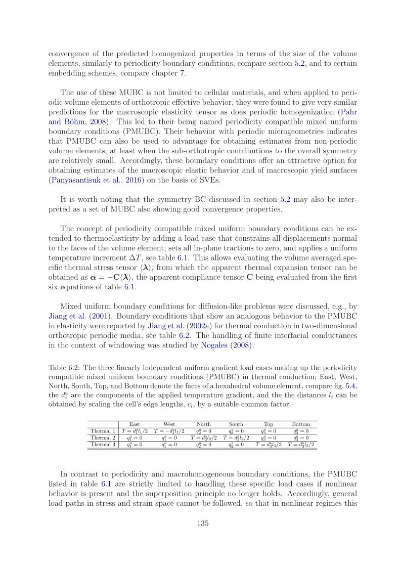
convergence of the predicted homogenized properties in terms of the size of the volumeelements, similarly to periodicity boundary conditions, compare section 5.2, and to certainembedding schemes, compare chapter 7.

The use of these MUBC is not limited to cellular materials, and when applied to peri-odic volume elements of orthotropic effective behavior, they were found to give very similarpredictions for the macroscopic elasticity tensor as does periodic homogenization (Pahrand Bohm, 2008). This led to their being named periodicity compatible mixed uniformboundary conditions (PMUBC). Their behavior with periodic microgeometries indicatesthat PMUBC can also be used to advantage for obtaining estimates from non-periodicvolume elements, at least when the sub-orthotropic contributions to the overall symmetryare relatively small. Accordingly, these boundary conditions offer an attractive option forobtaining estimates of the macroscopic elastic behavior and of macroscopic yield surfaces(Panyasantisuk et al., 2016) on the basis of SVEs.

It is worth noting that the symmetry BC discussed in section 5.2 may also be inter-preted as a set of MUBC also showing good convergence properties.

The concept of periodicity compatible mixed uniform boundary conditions can be ex-tended to thermoelasticity by adding a load case that constrains all displacements normalto the faces of the volume element, sets all in-plane tractions to zero, and applies a uniformtemperature increment ∆T , see table 6.1. This allows evaluating the volume averaged spe-cific thermal stress tensor 〈λ〉, from which the apparent thermal expansion tensor can beobtained as α = −C〈λ〉, the apparent compliance tensor C being evaluated from the firstsix equations of table 6.1.

Mixed uniform boundary conditions for diffusion-like problems were discussed, e.g., byJiang et al. (2001). Boundary conditions that show an analogous behavior to the PMUBCin elasticity were reported by Jiang et al. (2002a) for thermal conduction in two-dimensionalorthotropic periodic media, see table 6.2. The handling of finite interfacial conductancesin the context of windowing was studied by Nogales (2008).

Table 6.2: The three linearly independent uniform gradient load cases making up the periodicitycompatible mixed uniform boundary conditions (PMUBC) in thermal conduction; East, West,North, South, Top, and Bottom denote the faces of a hexahedral volume element, compare fig. 5.4,the dai are the components of the applied temperature gradient, and the the distances li can beobtained by scaling the cell’s edge lengths, ci, by a suitable common factor.

East West North South Top Bottom

Thermal 1 T = da

1l1/2 T = −da

1l1/2 qa

2= 0 qa

2= 0 qa

3= 0 qa

3= 0

Thermal 2 qa

1= 0 qa

1= 0 T = da

2l2/2 T = da

2l2/2 qa

3= 0 qa

3= 0

Thermal 3 qa

1= 0 qa

1= 0 qa

2= 0 qa

2= 0 T = da

3l3/2 T = da

3l3/2

In contrast to periodicity and macrohomogeneous boundary conditions, the PMUBClisted in table 6.1 are strictly limited to handling these specific load cases if nonlinearbehavior is present and the superposition principle no longer holds. Accordingly, generalload paths in stress and strain space cannot be followed, so that in nonlinear regimes this

135

type of model is restricted to materials characterization, compare (Pahr and Bohm, 2008).

Certain MUBC, e.g., ones that handle macroscopic uniaxial loading by specifying nor-mal displacements plus zero tangential tractions for one pair of faces and setting all tractioncomponents to zero for all other faces, compare, e.g., Galli et al. (2008), can be interpretedphysically as describing the behavior of small, inhomogeneous samples121 as discussed insection 1.5. Due to the weaker boundary constraints such sample-type (or “structure-type”) MUBC can be expected to predict more compliant macroscopic behavior than dothe periodicity boundary conditions discussed in section 5.2 or the PMUBC listed in table6.1. As mentioned in section 1.5, structure-type boundary conditions do not involve scaletransitions.

Important strengths of windowing methods lie in providing an approach to studyingthe behavior of non-periodic volume elements and in being considerably easier to handlethan PMAs for periodic volume elements. The main reasons for the latter point are thatthe meshing of homologous faces is not an issue in windowing and multi-point constraintequations are not required.

121In contrast to periodicity BC, these specific MUBC give different results for volume elements madeup of a number “base units” compared to models consisting of a single unit. This is in keeping with theirinterpretation as “structural” rather than “material” models.If the tangential strains rather than the tangential stresses are set to zero for the pair of faces controllingthe macroscopic axial deformation, the physical interpretation is that of a sample “sticking” to the baseplates, implying the presence of strain gradients at the length scale of the sample. Such models are notcapable of describing a proper uniaxial stress load case.

136

Chapter 7

Embedding Approaches and RelatedModels

Embedded Cell Approaches (ECAs) aim at predicting the microfields in specific, geomet-rically highly resolved (sub)regions of models of inhomogeneous materials or structures.Such models consist of two parts, as is evident in figs. 7.1 and 7.2. On the one hand, thereis a core (or “local heterogeneous region”) consisting of a discrete microstructure (“mo-tif”), which can range from rather simple to highly complex phase arrangements. On theother hand, there is a homogeneous outer region (“embedding region”, “frame”, “effectiveregion”) into which the core is embedded and which serves mainly for transmitting theapplied loads. Embedding strategies tend to give rise to relatively complex models, butthey avoid the main drawback of PMAs, viz., the requirement that the microgeometry andall microfields must be periodic.

An intrinsic feature of embedding models are boundary layers that occur at the “inter-faces” between the core and the embedding region and perturb the local stress and strainfields122, see, e.g., Harper et al. (2012a) and compare section 4.2. Provision must be madeto keep regions of specific interest, such as crack tips or process zones, at a sufficient dis-tance from the boundary layers123, which, in turn, implies that cores must exceed someminimum size in order to provide useful results.

Most of the embedding approaches reported in the literature for tasks related to con-tinuum micromechanics fall into two groups.

122The interfaces between core and embedding region are a consequence of the modeling approach anddo not have any physical background or significance. In elasticity such boundary layers typically have athickness of, say, the distance between the centers of neighboring inhomogeneities, but they may be longerranged for nonlinear material behavior.123Boundary layers and embedding regions may interfere with extended regions of concentrated strains,

with shear bands, or with the growth of damaged regions. Such difficulties can only be avoided or mitigatedby choosing a sufficiently large core region. In dynamic models the boundaries between core and embeddingregion may lead lead to the reflection and/or refraction of waves. Special transition layers can, however,be introduced to mitigate boundary layer effects in the latter case.

137

Embedding Region with Self-Consistently Determined Response

One group of embedding schemes employ the homogenized thermomechanical responseof the core for determining the effective behavior of the surrounding medium via self-consistent procedures. By applying suitable uniform far field loads to the outer boundariesof such an embedding layer, as sketched in Fig. 7.1, models of this type can be used forcarrying out scale transitions in terms of homogenization and, with some precautions,localization.

S.C.

embedding

core

Figure 7.1: Schematic depiction of the arrangement of core and embedding region in a self-consistent embedded cell model subjected to a uniform far-field load.

As mentioned in section 4.2 self-consistent embedding schemes employing macrohomo-geneous or periodic boundary conditions124 provide predictions for the effective elasticitytensors that lie between the lower and upper estimates on the apparent tensors and, byextension, within the mesoscale bounds discussed in chapter 6. Such approaches, in whichthe embedding layer mainly serves for smoothening out fluctuations at the core’s bound-aries have been termed the “Window Method” by some authors (Krabbenhøft et al., 2008;Temizer et al., 2013), and the designator “augmentation strip” was used for the embed-ding region in an earlier approach (Babuska et al., 1999). In a similar vein, the use of aself-consistent embedding “buffer layer” has been proposed for models in which periodicityboundary conditions are applied to non-periodic volume elements (Makowski et al., 2013).Methods of this type typically aim at carrying out scale transitions and, accordingly, thecore should approach a proper RVE as closely as possible.

124In such schemes either the full core (including the boundary layers) or core’s interior (the regionsaffected by the boundary layer being discarded) may be used for evaluating the effective responses. Intheir analysis of such self-consistent schemes (Temizer et al., 2013) take the former approach. For elasticspherical inhomogeneities in an elastic matrix the thickness of the boundary layer may be estimated asfour particle radii (Buryachenko, 2007).

138

Because they involve self-consistent iterations, self-consistent embedding methods tendto be more expensive numerically than are periodic homogenization and windowing anal-ysis (in the sense of chapter 6). In the elastic regime, however, the required number ofiterations tends to be fairly low and the approach has been shown to be unconditionallystable by Salit and Gross (2014). A number of issues in choosing the width of the embed-ding layer for thermoelastic analysis were discussed by Temizer et al. (2013).

The use of self-consistency procedures is, of course, predicated on the availability ofsuitable parameterizable constitutive laws for the embedding material that can follow thecore’s (instantaneous) homogenized behavior with high accuracy for all load cases andloading histories considered. This requirement can typically be fulfilled easily in the linearrange, see e.g., Yang et al. (1994) and Chen et al. (1994), but may lead to considerablecomplexity when at least one of the constituents shows elastoplastic or viscoplastic ma-terial behavior125. Accordingly, approximations may have to be used (the consequencesof which may be difficult to assess in view of the nonlinearity and path dependence ofsuch material behaviors) and models of this type are best termed “quasi-self-consistentschemes”. Approaches of this type were discussed, e.g., by Bornert et al. (1994) and byDong and Schmauder (1996).

Self-consistent and quasi-self-consistent embedding models are not suitable for handling“strong features”, such as localized cracks of the type shown in fig. 7.2, within the core andtheir physical interpretation may be difficult when the core includes subregions subject todamage.

Embedding Region with Prescribed Material Response

In the other group of embedding methods the material behavior of the outer region isdescribed via appropriate, pre-defined, “smeared-out” constitutive models. These typi-cally take the form of semi-empirical or micromechanically based constitutive laws thatare prescribed a priori for the embedding zone and are chosen to represent the appropriate(usually damage-free) material behavior126. This way, conceptually simple models are ob-

125Typically, the effective yielding behavior of elastoplastic composites shows some dependence on thefirst stress invariant, and, for low plastic strains, the homogenized response of the core tends to be stronglyinfluenced by the fractions of the elastoplastic constituent(s) that have actually yielded. In addition, inmany cases anisotropy of the yielding and hardening behavior is induced by the phase topology (e.g.,aligned fibers) and/or by the phase arrangement of the core. Identifying constitutive laws that, on the onehand, can satisfactorily account for such phenomena and, on the other hand, have the capability of beingeasily adapted to the instantaneous homogenized responses of the core by adjusting free parameters, posesa major challenge in applying self-consistent embedding schemes to nonlinear material behavior.126The constitutive model and the pertinent material parameters required for the embedding layer may

be obtained, e.g., from micromechanical modeling or from experiments (Ayyar et al., 2008).The description chosen for the embedding region must reflect the material symmetry, e.g., for metalmatrices reinforced by continuous fibers the yield surface, the flow rule and the hardening behavior mustaccount for these materials’ marked anisotropy in the elastoplastic regime.When the core is used for studying damage and failure, its boundary regions should be excluded from suchbehavior in order to avoid the perturbed stress and strain fields there. Furthermore, it is worth notingthat restricting failure or localized damage to the core may restrict the generality of models, compare, e.g.,Bao (1992).

139

tained that are very well suited to studying local phenomena such as the stress and straindistributions in the vicinity of crack tips (Aoki et al., 1996), around local defects (Xiaet al., 2001) or at macroscopic interfaces in composites (Chimani et al., 1997), the growthof cracks in inhomogeneous materials (van der Giessen and Tvergaard, 1994; Wulf et al.,1996; Motz et al., 2001; Mishnaevsky, 2004; Gonzalez and LLorca, 2007), or damage dueto the processing of composites (Monaghan and Brazil, 1997).

In applications of this type loads may be applied or displacement boundary conditionsmay be specified that impose a far field behavior obtained from a suitable analytical ornumerical solution (e.g., the displacements describing the far field of a crack tip in elas-ticity or small-scale plasticity) pertinent to the problem under study. Alternatively, theembedding region may be chosen to represent the structure or sample to be considered,with the core zooming in on a detail of special interest. Such approaches, which may beviewed as a type of concurrent multiscale modeling scheme, allow complete specimens orcomponents to be studied via “simulated experiments” as sketched in fig. 7.2.

Figure 7.2: Schematic depiction of the arrangement of core and embedding region in an embeddedcell model of a tensile test specimen.

Embedding models making use of prescribed properties for the embedding region arenot the best choice for homogenization analysis — they may rather be viewed as methodsspecialized towards localization. On the one hand, this arguably makes them the most ver-satile and powerful tool for looking in detail at “strong features” in some region of interest.Embedding models of this kind can be used without intrinsic restrictions at or in the vicin-ity of free surfaces and interfaces, they can handle gradients in composition and loads, andthey can be employed for studying the interaction of macrocracks with microstructures127.On the other hand, in such models the core in general is not required to be a proper RVE

127The requirement of sufficiently separated length scales, compare section 1.1, does not necessarily applyto embedded models. Care is, however, required, with highly nonlinear analyses, especially with modelsinvolving damage, where the inherent perturbations at boundaries between core and embedding regionmay trigger spurious behavior.

140

— in fact, it typically makes sense to use a volume element that is known to be critical forthe behavior to be studied, e.g., a crack tip or some specific microgeometrical feature. Itis worth noting that embedding models of this type do not involve scale transitions.

Other Embedding Strategies, Submodeling Schemes and RelatedApproaches

A further approach to embedding uses discrete microstructures in both the core region andin the surrounding material, the latter, however, being discretized by a much coarser FEmesh, see, e.g., Sautter et al. (1993). Such models, which are also referred to as “fine meshwindow” approaches (Podgorski, 2011) and are related to descriptions of full samples orstructures that contain a refined mesh in some region(s) of interest, can avoid boundarylayers to a considerable extent by using appropriately graded meshes. They tend, how-ever, to be rather expensive computationally. Mesh superposition techniques, which usea coarse mesh over the macroscopic model of some structure or sample together with ageometrically independent, much finer mesh in regions of interest (Takano et al., 2001) areconceptually similar to the above modeling strategy. Also, part of the embedding regionmay be modeled at similar resolution as the core and used as a “sacrificial region” servingto insulate the core from the boundary layer (Harper et al., 2012a).

A closely related approach makes use of submodeling techniques in which an inhomo-geneous micromodel is weakly or strongly coupled to a homogeneous macro model viaappropriate coupling conditions (which may, e.g., be implemented via the boundary condi-tions of the micromodel), compare, e.g., Heness et al. (1999) or Varadi et al. (1999). Also,far field strains obtained from an unperturbed periodic model subjected to an appropri-ate loading history may be used as boundary conditions for a region containing a localmicrostructural perturbation, compare Aboudi and Ryvkin (2012). Such approaches areconceptually related, on the one hand, to embedding models with prescribed embeddingbehavior as shown in Fig. 7.2 and, on the other hand, to the “inhomogeneous structuremodels” mentioned in section 1.5. The models mentioned here are more suitable for local-ization than for homogenization, the region with a highly resolved microgeometry beingbest chosen to correspond to a critical rather than a representative volume element. Whenstrongly perturbing features, such as crack tips, are present in the highly resolved region,it is important to make sure the model is large enough to prevent their interaction withits boundaries.

Additional Remarks on Embedding Schemes

When a periodic multi-inhomogeneity volume element is used as the core in a self-consistentor quasi-self-consistent embedding scheme, the concomitant relaxation of the periodicityconstraints tends to make the overall responses of the embedded configuration softer com-pared to periodic homogenization of the periodic arrangement alone (Bruzzi et al., 2001)128.

128In the study mentioned above, the difference between PMA and ECA results is relatively small.Identical responses can be expected from the two types of model if the core is described by a proper RVE

141

Some analytical methods such as classical and generalized self-consistent schemes, seesection 2.3, can obviously be viewed as embedding schemes that combine relatively simplecores with self-consistently defined material behavior of the embedding region. When geo-metrically more complex cores are considered in ECA-like frameworks, however, numericalengineering methods are best suited for resolving the discrete phase arrangements in thecore region, compare Bornert (1996).

The core and embedding regions may be planar, axisymmetric or fully three-dimensional,and symmetries present in the geometries can, as usual, be made us of for reducing thesize of the model, compare Xia et al. (2001). Effective and phase averaged stresses andstrains from embedded cell models are best evaluated via eqn. (1.4) or its equivalents, andit is typically good practice to use only the central regions of the core for this purpose inorder to avoid perturbations from the boundary layers.

All embedding techniques discussed above can also be used in analogy for studying thethermal conduction behavior of inhomogeneous materials.

(so that by definition the boundary conditions do not play a role) and the embedding material can fullydescribe the homogenized behavior of the core.

142

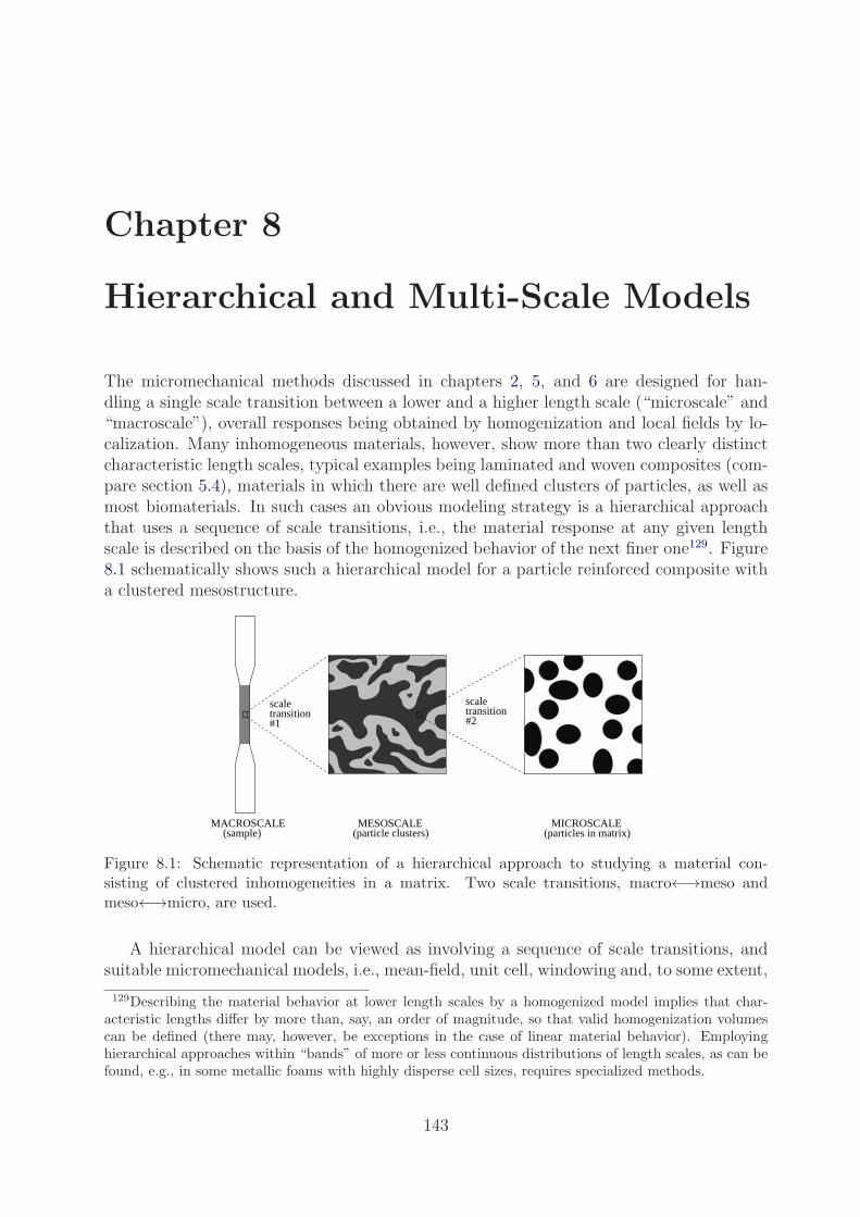
Chapter 8

Hierarchical and Multi-Scale Models

The micromechanical methods discussed in chapters 2, 5, and 6 are designed for han-dling a single scale transition between a lower and a higher length scale (“microscale” and“macroscale”), overall responses being obtained by homogenization and local fields by lo-calization. Many inhomogeneous materials, however, show more than two clearly distinctcharacteristic length scales, typical examples being laminated and woven composites (com-pare section 5.4), materials in which there are well defined clusters of particles, as well asmost biomaterials. In such cases an obvious modeling strategy is a hierarchical approachthat uses a sequence of scale transitions, i.e., the material response at any given lengthscale is described on the basis of the homogenized behavior of the next finer one129. Figure8.1 schematically shows such a hierarchical model for a particle reinforced composite witha clustered mesostructure.

transitionscale

#1transitionscale

#2

MACROSCALE(sample)

MESOSCALE(particle clusters)

MICROSCALE(particles in matrix)

Figure 8.1: Schematic representation of a hierarchical approach to studying a material con-sisting of clustered inhomogeneities in a matrix. Two scale transitions, macro←→meso andmeso←→micro, are used.

A hierarchical model can be viewed as involving a sequence of scale transitions, andsuitable micromechanical models, i.e., mean-field, unit cell, windowing and, to some extent,

129Describing the material behavior at lower length scales by a homogenized model implies that char-acteristic lengths differ by more than, say, an order of magnitude, so that valid homogenization volumescan be defined (there may, however, be exceptions in the case of linear material behavior). Employinghierarchical approaches within “bands” of more or less continuous distributions of length scales, as can befound, e.g., in some metallic foams with highly disperse cell sizes, requires specialized methods.

143

embedding approaches, may be used as “building blocks” at any level within hierarchicalschemes. Such hierarchical modeling strategies have the additional advantage of allowingthe behavior of the constituents at all lower length scales to be assessed via the corre-sponding localization relations. Multiscaling methods can be classified into concurrent andsequential approaches (Chakraborty and Rahman, 2008; Tadmor and Miller, 2011), withthe former requiring the physical problem to be studied simultaneously at all length scalesinvolved.

Among the continuum mechanical hierarchical descriptions of the thermomechanicalbehavior of inhomogeneous materials reported in the literature, some have combined mean-field methods at the higher length scale with mean-field (Hu et al., 1998; Tszeng, 1998) orperiodic microfield approaches (Gonzalez and LLorca, 2000) at the lower length scale. Acommon strategy for hierarchical modeling, however, uses Finite Element based unit cellor embedding methods at the topmost length scale, which implies that the homogenizedmaterial models describing the lower level(s) of the hierarchy must be proper constitutivelaws (i.e., material descriptions that are capable of handling any loading conditions and anyloading history) that are evaluated at each integration point of the discretized model. Forthis purpose, either explicit, micromechanically-based constitutive models may be used ormicromechanical models may be run at each integration point, the results of which provide“implicit” descriptions of the local material behavior. The models used for such purposesmay be analytical, semi-analytical or numerical.

For the elastic range, generating a micromechanically based constitutive description ateach integration point of the “macroscopic” model typically does not pose massive com-putational requirements130 — once the appropriate homogenized elasticity and thermalconcentration tensors have been generated any load case can be handled, often in a se-quential mode. For simulating the thermomechanical response of inelastic inhomogeneousmaterials, however, essentially a full micromechanical submodel has to be maintained andsolved for at each integration point, which amounts to fully concurrent procedures131. Al-though within such frameworks the use of sophisticated numerical models at the lowerlength scales tends to be an expensive proposition in terms of computational requirements,this concept has elicited major research interest, especially within the framework of multi-scale models (Belsky et al., 1995; Ghosh et al., 1996; Lee and Ghosh, 1996; Zohdi et al.,1996; Smit et al., 1998; Feyel and Chaboche, 2000; Fish and Shek, 2000; Ibrahimbegovicand Markovic, 2003; Moes et al., 2003; Tan et al., 2020). Pertinent overviews were givenby Ghosh et al. (2001), Kanoute et al. (2009), Geers et al. (2010) as well as Nguyen et al.(2011).

130Decomposition techniques can be used to formulate the problems at the finer length scales in such away that they are well suited for parallel processing, allowing the development of computationally highlyefficient multi-scale procedures, see, e.g., Oden and Zohdi (1997).131Some approaches have been reported that aim at decoupling the scales by parameterizing results from

microscopic unit cell analysis and using this data together with an interpolation scheme as an “approximateconstitutive model”, see, e.g., Terada and Kikuchi (1996), Ganser (1998) or Schrefler et al. (1999). Amajor challenge in this type of sequential modeling strategy lies in handling load history and load pathdependences required to account for elastoplastic local behavior of and/or microscopic damage to theconstituents. Appropriate representation of general multiaxial stress and/or strain states also tends to bedifficult.

144

It is worth noting that in models of this type (which are often referred to as FE2 pro-cedures) no explicit material law is used on the macroscale, the full constitutive behaviorbeing determined concurrently at the microscale. Arguably, such approaches at presentrepresent the most sophisticated application of the concepts of continuum micromechanics.

Lower (but by no means negligible) computational costs can be achieved by using mean-field models in lieu of constitutive models at the integration point level. Applications toelastoplastic composites have included incremental Mori–Tanaka methods, see, e.g., Petter-mann (1997) and mean-field based versions of the Transformation Field Analysis, compare,e.g., Fish and Shek (1998) or Plankensteiner (2000). In addition, the semi-analytical non-uniform TFA has been employed for this purpose (Michel and Suquet, 2004). Figure 8.2shows a result obtained by applying a multiscale approach that uses an incremental Mori–Tanaka method, compare section 2.5, at the integration point level of a two-dimensionalmeso-scale unit cell model for describing the elastoplastic behavior of a cluster-structuredhigh speed steel. The particle-rich and particle-poor regions used for the description at themesoscale are treated as particle reinforced MMCs with appropriate reinforcement volumefractions. Such a model not only predicts macroscopic stress–strain curves, but also al-lows the mesoscopic distributions of phase averaged microscopic variables to be evaluated,compare (Plankensteiner, 2000). For an example of an Extended Finite Element methodat the upper length scale coupled to a semi-analytical model at the lower one see Novaket al. (2012).

EPS.EFF.PLAST.MTX.

3.5000E-03

3.0000E-03

2.5000E-03

2.0000E-03

1.5000E-03

SCALAR MIN: -6.8514E-04SCALAR MAX: 1.3667E-02

Figure 8.2: Phase averaged microscopic equivalent plastic strains in the matrix within theinhomogeneity-poor regions of a cluster-structured high speed steel under mechanical loadingas predicted by a mesoscopic unit cell model combined with an incremental Mori–Tanaka modelat the microscale (Plankensteiner, 2000).

Alternatively, multiscale approaches may be rather “loosely coupled”, essentially link-ing together quite different models to obtain an overall result, see, e.g., (Onck and van derGiessen, 1997).

A further development are concurrent multi-scale methods in which the computational

145

domain is adaptively split into regions resolved at the appropriate length scale. In an FE-based hierarchical framework developed by Ghosh et al. (2001) “non-critical” regions aredescribed by continuum elements with pre-homogenized material properties, and for zonesof clearly nonlinear behavior PMA models are automatically activated at the integrationpoints to monitor the phase behavior at the microscale. If local behavior exceeding thecapabilities of periodic homogenization is detected (e.g., progressive damage, mesoscopicinterfaces, free edges), embedded models of the fully resolved microgeometry may be acti-vated at the appropriate positions, compare Raghavan and Ghosh (2004). Such strategiesallow detailed studies of critical regions in inhomogeneous materials, e.g., near free edges.In an alternative approach, homogenization models employing generalized continua havebeen proposed for handling regions close to free surfaces and zones with high local fieldgradients (Feyel, 2003).

Finally, it is worth noting that hierarchical and multi-scale approaches are not limitedto using the “standard” methods of continuum micromechanics as discussed above. Espe-cially the capability of the Finite Element method of handling highly complex constitutivedescriptions has been used to build hierarchical approaches that employ, among others,material models based on crystal plasticity (McHugh et al., 1993) and discrete dislocationplasticity (Cleveringa et al., 1997).

The linking of continuum and atomistic descriptions has been an important goal of mod-eling work for a considerable time, involving, e.g., concurrent homogenization schemes,compare Curtin and Miller (2003) and, for a view on recent and future developments,van der Giessen et al. (2020). The equivalent of homogenization in such settings is oftenreferred to as “upwards linking”, that to localization being known as “downward linking”.

146

Chapter 9

Closing Remarks

The research field of continuum micromechanics of materials has enjoyed considerable suc-cess in the past four decades in furthering the understanding of the thermomechanicalbehavior of inhomogeneous materials and in providing predictive tools for engineers andmaterials scientists. However, its methods are subject to some practical limitations thatshould be kept in mind when employing them.

All the methods discussed in chapters 2 to 6 implicitly use the assumption that theconstituents of the inhomogeneous material to be studied can be treated as homogeneousat the lower length scale, which, of course, does not necessarily hold. When the length scaleof the inhomogeneities in a constituent is much smaller than the length scale of the phasearrangement to be studied, the above assumption is valid and hierarchical as well as multi-scale models (“successive homogenization”) as discussed in chapter 8 can be used (Carrere,2001). However, no rigorous theory appears to be available at present for handling scaletransitions in materials that do not fulfill the above requirement (e.g., particle reinforcedcomposites in which the grain size of the matrix is comparable to or even larger than thesize of the particles132). Typically the best that can be done in such cases is either to usesufficiently detailed models with resolved microgeometry (potentially, a computationallyvery expensive proposition) or to employ homogenized phase properties and be aware ofthe approximation that is introduced.

A major practical difficulty in the use of continuum micromechanics approaches (whichin many cases is closely related to the questions mentioned above) has been identifyingappropriate constitutive models and obtaining the required material parameters for theconstituents. Typically, available data pertain to the behavior of the bulk materials (asmeasured from homogeneous macroscopic samples), whereas the actual requirement is forparameters and, in some cases, constitutive theories that describe the in-situ response ofthe constituents at the microscale. For example, with respect to MMCs, on the one hand,there is considerable evidence that classical continuum plasticity theories (in which thereis no absolute length scale) cannot adequately describe the behavior of metallic materi-als in the presence of strong strain gradients, where geometrically necessary dislocationscan markedly influence the material behavior (Hutchinson, 2000). On the other hand,

132For this special case unit cell or embedding models employing anisotropic or crystal plasticity modelsfor the phases may be used which, however, can become very large when the statistics of grain orientationare accounted for.

147

it is well known that the presence of reinforcements can lead to accelerated aging andrefinement of the grain size in the matrix (“secondary strengthening”). Furthermore, inmany cases reasonably accurate material parameters are essentially not available (e.g.,strength parameters for most interfaces in inhomogeneous materials). In fact, the dearthof dependable material parameters is one of the reasons why predictions of the strength ofinhomogeneous materials by micromechanical methods tend to be a considerable challenge.

Another point that should be kept in mind is that continuum micromechanical descrip-tions in most cases do not have absolute length scales unless a length scale is introducedexplicitly, typically via the constitutive model(s) of one (or more) of the constituents133.In this vein, absolute length scales, on the one hand, may be provided explicitly via dis-crete dislocation models (Cleveringa et al., 1997), via gradient or nonlocal constitutivelaws, see, e.g., Tomita et al. (2000) or Niordson and Tvergaard (2001), or via (nonlocal)damage models. On the other hand, they may be introduced in an ad-hoc fashion, e.g.,by adjusting the phase material parameters to account for grain sizes via the Hall–Petcheffect. Analysts should also be aware that absolute length scales may be introduced in-advertently into a model by mesh dependence effects of discretizing numerical methods, a“classical” example being strain localization due to softening material behavior of a con-stituent. When hierarchical or multi-scale models are used special care may be necessaryto avoid introducing inconsistent length scales at different modeling levels.

In addition it is worth noting that usually the macroscopic responses of inhomoge-neous materials (and, as a consequence of eqns. (2.8) to (2.14), the phase averages of themicrofields) are much less sensitive to the phase arrangement (and to modeling approxima-tions) than are the distributions of the microfields. Accordingly, whereas good agreementin the overall behavior of a given model with “benchmark” theoretical results or experimen-tal data typically indicates that the phase averages of stresses and strains are describedsatisfactorily, this does not necessarily imply that the higher statistical moments of thestress and strain distributions (and thus the heterogeneity of these fields) are capturedsufficiently accurately.

It is important to be aware that work in the field of micromechanics of materials invari-ably involves finding viable compromises in terms of the complexity of the models, which,on the one hand, have to be able to account (at least to a reasonably good approximation)for the physical phenomena relevant to the given problem, and, on the other hand, must besufficiently simple to allow solutions to be obtained within the relevant constraints of time,cost, and computational resources. Obviously, actual problems cannot be solved withoutrecourse to various approximations and tradeoffs — the important point is to be aware ofthem and to account for them in interpreting and assessing results. It is worth keeping inmind that there is no such thing as a “best micromechanical approach” to all problems.

133One important exception are models for studying macroscopic cracks (e.g., via embedded cells), wherethe crack length does introduce an absolute length scale.It is worth noting that the behavior of nanocomposites is typically dominated by interfaces (or interphases).Appropriately accounting for this behavior may require the introduction of an absolute length scale. Withinthe framework of mean-field methods this may be achieved by introducing surface terms into the Eshelbytensor, see, e.g., Duan et al. (2005).

148

Bibliography

N. Abolfathi, A. Naik, G. Karami, and C. Ulven. A micromechanical characterization ofangular bidirectional fibrous composites. Comput.Mater.Sci., 43:1193–1206, 2008.

J. Aboudi. The generalized method of cells and high-fidelity generalized method of cellsmicromechanical models — A review. Mech.Adv.Mater.Struct., 11:329–366, 2004.

J. Aboudi. Damage in composites — modeling of imperfect bonding. Compos.Sci.Technol.,28:103–128, 1987.

J. Aboudi. Micromechanical analysis of composites by the method of cells. Appl.Mech.Rev.,42:193–221, 1989.

J. Aboudi. Mechanics of Composite Materials. Elsevier, Amsterdam, 1991.

J. Aboudi. Micromechanical analysis of composites by the method of cells — Update.Appl.Mech.Rev., 49:S83–S91, 1996.

J. Aboudi and M. Ryvkin. The effect of localized damage on the behavior of compositeswith periodic microstructure. Int.J.Engng.Sci., 52:41–55, 2012.

D.W. Abueidda, M. Bakir, A.K. Abu Al-Rub, J.S. Bergstrom, N.A. Sobh, and I. Jasiuk.Mechanical properties of 3D printed polymer cellular materials with triply periodic min-imal surface architectures. Mater.Design, 122:255–267, 2017.

M.L. Accorsi. A method for modeling microstructural material discontinuities in a finiteelement analysis. Int.J.Num.Meth.Engng., 26:2187–2197, 1988.

J.D. Achenbach and H. Zhu. Effect of interfacial zone on mechanical behavior and failureof fiber-reinforced composites. J.Mech.Phys.Sol., 37:381–393, 1989.

D.F. Adams and D.A. Crane. Finite element micromechanical analysis of a unidirectionalcomposite including longitudinal shear loading. Comput.Struct., 18:1153–1165, 1984.

D.F. Adams and D.R. Doner. Transverse normal loading of a uni-directional composite.J.Compos.Mater., 1:152–164, 1967.

S.G. Advani and C.L. Tucker. The use of tensors to describe and predict fiber orientationin short fiber composites. J.Rheol., 31:751–784, 1987.

D.H. Allen and J.W. Lee. The effective thermoelastic properties of whisker-reinforcedcomposites as functions of material forming parameters. In G.J. Weng, M. Taya, andH. Abe, editors, Micromechanics and Inhomogeneity, pages 17–40, New York, NY, 1990.Springer-Verlag.

149

H. Altendorf and D. Jeulin. Random-walk-based stochastic modeling of three-dimensionalfiber systems. Phys.Rev. E, 83:041804, 2011.

A. Anthoine. Derivation of the in-plane elastic characteristics of masonry through homog-enization theory. Int.J.Sol.Struct., 32:137–163, 1995.

T. Antretter. Micromechanical Modeling of High Speed Steel. Reihe 18, Nr. 232. VDI–Verlag, Dusseldorf, 1998.

S. Aoki, Y. Moriya, K. Kishimoto, and S. Schmauder. Finite element fracture analysis ofWC–Co alloys. Engng.Fract.Mech., 55:275–287, 1996.

P. Arbenz, G.H. van Lenthe, U. Mennel, R. Muller, and M. Sala. Multi-level µ-finiteelement analysis for human bone structures. In B. Kagstrom, E. Elmroth, J. Dongarra,and J. Wasniewski, editors, Applied Parallel Computing. State of the Art in ScientificComputing, pages 240–250, Berlin, 2008. Springer-Verlag.

R.T. Arenburg and J.N. Reddy. Analysis of metal-matrix composite structures — I. Mi-cromechanics constitutive theory. Comput.Struct., 40:1357–1368, 1991.

J.L. Auriault. Upscaling heterogeneous media by asymptotic expansions. J.Engng.Mech.,128:817–822, 2002.

J.L. Auriault. Effective macroscopic description for heat conduction in periodic composites.Int.J.Heat Mass Transf., 26:861–869, 1983.

M. Avellaneda. Iterated homogenization, differential effective medium theory, and appli-cations. Comm.Pure Appl.Math., 40:803–847, 1987.

M. Avellaneda and G.W. Milton. Optimal bounds on the effective bulk modulus of poly-crystals. J.Appl.Math., 49:824–837, 1989.

M.S. Axelsen and R. Pyrz. Correlation between fracture toughness and the microstruc-ture morphology in transversely loaded unidirectional composites. In R. Pyrz, editor,Microstructure–Property Interactions in Composite Materials, pages 15–26, Dordrecht,1995. Kluwer Academic Publishers.

A. Ayyar, G.A. Crawford, J.J. Williams, and N. Chawla. Numerical simulation of the effectof particle spatial distribution and strength on tensile behavior of particle reinforcedcomposites. Comput.Mater.Sci., 44:496–506, 2008.

I. Babuska, B. Andersson, P.J. Smith, and K. Levin. Damage analysis of fiber composites.Part I: Statistical analysis on fiber scale. Comput.Meth.Appl.Mech.Engng., 172:27–77,1999.

Y. Bai, C.Z. Dong, and Z.Y. Liu. Effective elastic properties and stress states of dou-bly periodic array of inclusions with complex shapes by isogeometric boundary elementmethod. Compos.Struct., 128:54–69, 2015.

D. Balzani, D. Brands, J. Schroder, and C. Carstensen. Sensitivity analysis of statisticalmeasurements for the reconstruction of microstructures based on the minimization ofgeneralized least-square functionals. Techn.Mech., 30:297–315, 2010.

150

P.K. Banerjee and D.P. Henry. Elastic analysis of three-dimensional solids with fiberinclusions by BEM. Int.J.Sol.Struct., 29:2423–2440, 1992.

L. Banks-Sills and V. Leiderman. Macro-mechanical material model for fiber-reinforcedmetal matrix composites. Composites B, 30:443–452, 1999.

Y. Bansal and M.J. Pindera. Finite-volume direct averaging micromechanics of heteroge-neous materials with elastic-plastic phases. Int.J.Plast., 22:775–825, 2006.

G. Bao. Damage due to fracture of brittle reinforcements in a ductile matrix. Acta.metall.mater., 40:2547–2555, 1992.

G. Bao, J.W. Hutchinson, and R.M. McMeeking. Particle reinforcement of ductile matricesagainst plastic flow and creep. Acta metall.mater., 39:1871–1882, 1991.

R.B. Barello and M. Levesque. Comparison between the relaxation spectra obtainedfrom homogenization models and finite elements simulation for the same composite.Int.J.Sol.Struct., 45:850–867, 2008.

S. Bargmann, B. Klusemann, J. Markmann, J.E. Schnabel, K. Schneider, C. Soyarslan,and J. Wilmers. Generation of 3D representative volume elements for heterogeneousmaterials: A review. Prog.Mater.Sci., 96:322–384, 2018.

B. Barroqueiro, J. Dias-de Oliveira, J. Pinho-da Cruz, and A. Andrade-Campos. Practi-cal implementation of asymptotic expansion homogenisation in thermoelasticity using acommercial simulation software. Compos.Struct., 141:117–131, 2016.

N.D. Barulich, L.A. Godoy, and P.M. Dardati. A simple procedure to evaluate Cauchystress tensor at the macro level based on computational micromechanics under generalfinite strain states. Mech.Mater., 117:73–80, 2018.

J.L. Bassani, A. Needleman, and E. van der Giessen. Plastic flow in a composite: Com-parison of nonlocal continuum and discrete dislocation predictions. Int.J.Sol.Struct., 38:833–853, 2001.

V. Belsky, M.W. Beall, J. Fish, M.S. Shephard, and S. Gomaa. Computer-aided multiscalemodeling tools for composite materials and structures. Comput.Syst.Engng., 6:213–223,1995.

Y. Benveniste. A new approach to the application of Mori–Tanaka’s theory in compositematerials. Mech.Mater., 6:147–157, 1987.

Y. Benveniste. Some remarks on three micromechanical models in composite media.J.Appl.Mech., 57:474–476, 1990.

Y. Benveniste and G.J. Dvorak. On a correspondence between mechanical and thermaleffects in two-phase composites. In G.J. Weng, M. Taya, and H. Abe, editors, Microme-chanics and Inhomogeneity, pages 65–82, New York, NY, 1990. Springer-Verlag.

Y. Benveniste, G.J. Dvorak, and T. Chen. On diagonal and elastic symmetry of theapproximate effective stiffness tensor of heterogeneous media. J.Mech.Phys.Sol., 39:927–946, 1991.

151

A.A. Benzerga and J. Besson. Plastic potentials for anisotropic porous solids.Eur.J.Mech. A/Solids, 20:397–434, 2001.

M.J. Beran and J. Molyneux. Use of classical variational principles to determine boundsfor the effective bulk modulus in heterogeneous media. Quart.Appl.Math., 24:107–118,1966.

S.A. Berggren, D. Lukkassen, A. Meidell, and L. Simula. Some methods for calculatingstiffness properties of periodic structures. Appl.Math, 2:97–110, 2003.

J.G. Berryman. Long-wavelength propagation in composite elastic media, II. Ellipsoidalinclusions. J.Acoust.Soc.Amer., 68:1820–1831, 1980.

J.G. Berryman and P.A. Berge. Critique of two explicit schemes for estimating elasticproperties of multiphase composites. Mech.Mater., 22:149–164, 1996.

J.G. Berryman and G.W. Milton. Microgeometry of random composites and porous media.J. Phys.D, 21:87–94, 1988.

M. Berveiller and A. Zaoui. A simplified self-consistent scheme for the plasticity of two-phase metals. Res.Mech.Lett., 1:119–124, 1981.

A. Bhattacharyya and G.J. Weng. Plasticity of isotropic composites with randomly orientedpacketed inclusions. Int.J.Plast., 10:553–578, 1994.

P. Bisegna and R. Luciano. Variational bounds for the overall properties of piezoelectriccomposites. J.Mech.Phys.Sol., 44:583–602, 1996.

J.E. Bishop, J.M. Emery, R.V. Field, C.R. Weinberger, and D.J. Littlewood. Direct numer-ical simulations in solid mechanics for understanding the macroscale effects of microscalematerial variability. Comput.Mech.Appl.Mech.Engng., 287:262–289, 2015.

J.F.W. Bishop and R. Hill. A theory of the plastic distortion of a polycrystalline aggregateunder combined stress. London Edinburgh Dublin Phil.Mag.J.Sci., 42:414–427, 1951.

B. Bochenek and R. Pyrz. Reconstruction of random microstructures — a stochasticoptimization problem. Comput.Mater.Sci., 31:93–112, 2004.

H.J. Bohm. A short introduction to continuum micromechanics. In H.J. Bohm, editor,Mechanics of Microstructured Materials, pages 1–40. Springer-Verlag, CISM Courses andLectures Vol. 464, 2004.

H.J. Bohm. Comparison of analytical and numerical models for the thermoelastic behaviorof composites reinforced by coated spheres. Int.J.Engng.Sci., 142:216–229, 2019.

H.J. Bohm and W. Han. Comparisons between three-dimensional and two-dimensionalmulti-particle unit cell models for particle reinforced metal matrix composites. Mod-ell.Simul.Mater.Sci.Engng., 9:47–65, 2001.

H.J. Bohm and F.G. Rammerstorfer. Fiber arrangement effects on the microscale stresses ofcontinuously reinforced MMCs. In R. Pyrz, editor, Microstructure–Property Interactionsin Composite Materials, pages 51–62, Dordrecht, 1995. Kluwer Academic Publishers.

152

H.J. Bohm and A. Rasool. Effects of particle shape on the thermoelastoplastic behaviorof particle reinforced composites. Int.J.Sol.Struct., 87:90–101, 2016.

H.J. Bohm, F.G. Rammerstorfer, and E. Weissenbek. Some simple models for microme-chanical investigations of fiber arrangement effects in MMCs. Comput.Mater.Sci., 1:177–194, 1993.

H.J. Bohm, A. Eckschlager, and W. Han. Modeling of phase arrangement effects in highspeed tool steels. In F. Jeglitsch, R. Ebner, and H. Leitner, editors, Tool Steels in theNext Century, pages 147–156, Leoben, 1999. Montanuniversitat Leoben.

H.J. Bohm, A. Eckschlager, and W. Han. Multi-inclusion unit cell models for metal matrixcomposites with randomly oriented discontinuous reinforcements. Comput.Mater.Sci.,25:42–53, 2002.

H.J. Bohm, D.H. Pahr, and T. Daxner. Analytical and numerical methods for modelingthe thermomechanical and thermophysical behavior of microstructured materials. InV.V. Silberschmidt, editor, Computational and Experimental Mechanics of AdvancedMaterials, pages 167–223. Springer-Verlag, CISM Courses and Lectures Vol. 514, 2009.

N. Bonfoh, V. Hounkpati, and H. Sabar. New micromechanical approach of the coatedinclusion problem: Exact solution and applications. Comput.Mater.Sci., 62:175–183,2012.

M. Bornert. Homogeneisation des milieux aleatoires: Bornes et estimations. In M. Bornert,T. Bretheau, and P. Gilormini, editors, Homogeneisation en mecanique des materiaux1. Materiaux aleatoires elastiques et milieux periodiques, pages 133–221, Paris, 2001.Editions Hermes.

M. Bornert. Morphologie microstructurale et comportement mecanique; characterisationsexperimentales, approches par bornes et estimations autocoherentes generalisees. PhDthesis, Ecole Nationale des Ponts et Chaussees, Paris, 1996.

M. Bornert and P. Suquet. Proprietes non lineaires des composites: Approches par lespotentiels. In M. Bornert, T. Bretheau, and P. Gilormini, editors, Homogeneisation enmecanique des materiaux 2. Comportements non lineaires et problemes ouverts, pages45–90, Paris, 2001. Editions Hermes.

M. Bornert, E. Herve, C. Stolz, and A. Zaoui. Self consistent approaches and strainheterogeneities in two-phase elastoplastic materials. Appl.Mech.Rev., 47:66–S76, 1994.

M. Bornert, C. Stolz, and A. Zaoui. Morphologically representative pattern-based boundingin elasticity. J.Mech.Phys.Sol., 44:307–331, 1996.

M. Bornert, T. Bretheau, and P. Gilormini, editors. Homogeneisation en mecanique desmateriaux. Editions Hermes, Paris, 2001.

D. Boussaa. Effective thermoelastic properties of composites with temperature-dependentconstituents. Mech.Mater., 43:397–407, 2011.

S. Boyd and R. Muller. Smooth surface meshing for automated finite element modelgeneration from 3D image data. J.Biomech., 39:1287–1295, 2006.

153

L. Brassart, L. Stainier, I. Doghri, and L. Delannay. Homogenization of elasto-(visco)plasticcomposites based on an incremental variational principle. Int.J.Plast., 36:86–112, 2012.

R. Brenner and R. Masson. Improved affine estimates for nonlinear viscoelastic composites.Eur.J.Mech. A/Solids, 24:1002–1015, 2005.

R. Brenner, O. Castelnau, and P. Gilormini. A modified affine theory for the overallproperties of nonlinear composites. C.R.Acad.Sci.Paris, serie IIb, 329:649–654, 2001.

L.C. Brinson and W.S. Lin. Comparison of micromechanics methods for effective propertiesof multiphase viscoelastic composites. Compos.Struct., 41:353–367, 1998.

S. Brisard and L. Dormieux. FFT-based methods for the mechanics of composites: Ageneral variational framework. Comput.Mater.Sci., 49:663–671, 2010.

L.M. Brown and W.M. Stobbs. The work-hardening of copper–silica. I. A model based oninternal stresses, with no plastic relaxation. Phil.Mag., 23:1185–1199, 1971.

D.A.G. Bruggemann. Berechnung verschiedener physikalischer Konstanten von heteroge-nen Substanzen. I. Dielektrizitatskonstanten und Leitfahigkeiten der Mischkorper ausisotropen Substanzen. Ann.Phys., 24:636–679, 1935.

M.S. Bruzzi, P.E. McHugh, F. O’Rourke, and T. Linder. Micromechanical modelling ofthe static and cyclic loading of an Al 2141-SiC MMC. Int.J.Plast., 17:565–599, 2001.

I. Bucataru and M.A. Slawinski. Invariant properties for finding distance in space ofelasticity tensors. J.Elast., 94:97–114, 2009.

J.Y. Buffiere, P. Cloetens, W. Ludwig, E. Maire, and L. Salvo. In situ X-ray tomographystudies of microstructural evolution combined with 3D modeling. MRS Bull., 33:611–619,2008.

V.N. Bulsara, R. Talreja, and J. Qu. Damage initiation under transverse loading of uni-directional composites with arbitrarily distributed fibers. Compos.Sci.Technol., 59:673–682, 1999.

V. Buryachenko. Micromechanics of Heterogeneous Materials. Springer-Verlag. Berlin,2007.

V. Buryachenko. Local and Nonlocal Micromechanics of Heterogeneous Materials. Springer-Verlag. Cham, 2022.

V.A. Buryachenko. The overall elastoplastic behavior of multiphase materials with isotropiccomponents. Acta Mech., 119:93–117, 1996.

V.A. Buryachenko and A.M. Lipanov. Stress concentration at ellipsoidal inclusions andeffective thermoelastic properties of composite materials. Sov.Appl.Mech., 22:1103–1109,1986.

V.A. Buryachenko, N.J. Pagano, R.Y. Kim, and J.E. Spowart. Quantitative descriptionand numerical simulation of random microstructures of composites and their elasticmoduli. Int.J.Sol.Struct., 40:47–72, 2003.

154

J. Bystrom, N. Jekabsons, and J. Varna. An evaluation of different models for predictionof elastic properties of woven composites. Composites B, 31:7–20, 2000.

C.W. Camacho, C.L. Tucker, S. Yalvac, and R.L. McGee. Stiffness and thermal expansionpredictions for hybrid short fiber composites. Polym.Compos., 11:229–239, 1990.

N. Carrere. Sur l’analyse multiechelle des materiaux composites a matrice metallique:application au calcul de structure. PhD thesis, Ecole Polytechnique, Palaiseau, 2001.

M.A.A. Cavalcante, M.J. Pindera, and H. Khatam. Finite-volume micromechanics of pe-riodic materials: Past, present and future. Composites B, 43:2521–2543, 2012.

A. Cazzani and M. Rovati. Extrema of Young’s modulus for cubic and transversely isotropicsolids. Int.J.Sol.Struct., 40:1713–1744, 2003.

J.L. Chaboche and P. Kanoute. Sur les approximations “isotrope” et “anisotrope” del’operateur tangent pour les methodes tangentes incrementale et affine. C.R.Mecanique,331:857–864, 2003.

J.L. Chaboche, S. Kruch, J.F. Maire, and T. Pottier. Towards a micromechanics basedinelastic and damage modelling of composites. Int.J.Plast., 17:411–439, 2001.

A. Chakraborty and S. Rahman. Stochastic multiscale models for fracture analysis offunctionally graded materials. Engng.Fract.Mech., 75:2062–2068, 2008.

N. Charalambakis. Homogenization techniques and micromechanics. A survey and per-spectives. Appl.Mech.Rev., 63:030803, 2010.

G. Chatzigeorgiou and F. Meraghni. Elastic and inelastic local strain fields in compositeswith coated fibers or particles: Theory and validation. Math.Mech.Sol., 24:2858–2894,2019.

N. Chawla and K.K. Chawla. Microstructure based modeling of the deformation behaviorof particle reinforced metal matrix composites. J.Mater.Sci., 41:913–925, 2006.

H.R. Chen, Q.S. Yang, and F.W. Williams. A self-consistent finite element approach tothe inclusion problem. Comput.Mater.Sci., 2:301–307, 1994.

Q. Chen, X. Chen, Z. Zhai, and Z. Yang. A new and general formulation of three-dimensional finite-volume micromechanics for particulate reinforced composites withviscoplastic phases. Composites B, 85:216–232, 2016.

T. Chen. Exact moduli and bounds of two-phase composites with coupled multifield linearresponses. J.Mech.Phys.Sol., 45:385–398, 1997.

B. Chiaia, A. Vervuurt, and J.G.M. van Mier. Lattice model evaluation of progressivefailure in disordered particle composites. Engng.Fract.Mech., 57:301–318, 1997.

C.M. Chimani, H.J. Bohm, and F.G. Rammerstorfer. On stress singularities at free edgesof bimaterial junctions — A micromechanical study. Scr.mater., 36:943–947, 1997.

R.M. Christensen. Sufficient symmetry conditions for isotropy of the elastic moduli tensor.J.Appl.Mech., 54:772–777, 1987.

155

R.M. Christensen. Two theoretical elasticity micromodels. J.Elast., 50:15–25, 1998.

R.M. Christensen and K.H. Lo. Solutions for effective shear properties in three phasesphere and cylinder models. J.Mech.Phys.Sol., 27:315–330, 1979.

R.M. Christensen and K.H. Lo. Erratum to Christensen and Lo, 1979. J.Mech.Phys.Sol.,34:639, 1986.

R.M. Christensen, H. Schantz, and J. Shapiro. On the range of validity of the Mori–Tanakamethod. J.Mech.Phys.Sol., 40:69–73, 1992.

B.G. Christoff, H. Brito-Santana, S. Talreja, and V. Tita. Development of an ABAQUSTM

plug-in to evaluate the fourth-order elasticity tensor of a periodic material via homoge-nization by the asymptotic expansion method. Fin.Elem.Anal.Design, 181:103482, 2020.

P.W. Chung, K.K. Tamma, and R.R. Namburu. Asymptotic expansion homogenizationfor heterogeneous media: Computational issues and applications. Composites A, 32:1291–1301, 2001.

H.H.M. Cleveringa, E. van der Giessen, and A. Needleman. Comparison of discrete dislo-cation and continuum plasticity predictions for a composite material. Acta mater., 45:3163–3179, 1997.

T.W. Clyne and P.J. Withers. An Introduction to Metal Matrix Composites. CambridgeUniversity Press, Cambridge, 1993.

I. Cohen. Simple algebraic approximations for the effective elastic moduli of cubic arraysof spheres. J.Mech.Phys.Sol., 52:2167–2183, 2004.

D.A. Colera and H.G. Kim. Asymptotic expansion homogenization analysis using two-phase representative volume element for non-periodic composite materials. Mul-tisc.Sci.Engng., 1:130–140, 2019.

R.D. Cook and W.C. Young. Advanced Mechanics of Materials. Mcmillan, London, 1985.

W.M.G. Courage and P.J.G Schreurs. Effective material parameters for composites withrandomly oriented short fibers. Comput.Struct., 44:1179–1185, 1992.

B.N. Cox and G. Flanagan. Handbook of analytical methods for textile composites. Tech-nical Report NASA–CR–4570, NASA, Washington, DC, 1997.

H.L. Cox. The elasticity and strength of paper and other fibrous materials. Brit.J.Appl.Phys., 3:72–79, 1952.

M.E. Cruz and A.T. Patera. A parallel Monte-Carlo finite element procedure for theanalysis of multicomponent random media. Int.J.Num.Meth.Engng., 38:1087–1121, 1995.

J. Cugnoni and M. Galli. Representative volume element size of elastoplastic andelastoviscoplastic particle-reinforced composites with random microstructure. Com-put.Model.Engng.Sci., 66:165–185, 2010.

W.A. Curtin and R.E. Miller. Atomistic/continuum coupling in computational materialsscience. Model.Simul.Mater.Sci.Engng., 11:R33–R68, 2003.

156

A.S. Dalaq, D.W. Abueidda, R. Abu Al-Rub, and I.M. Jasiuk. Finite element predictionsof effective elastic properties of interpenetrating phase composites with architecturedsheet reinforcements. Int.J.Sol.Struct., 83:169–182, 2016.

T.D. Dang and B.V. Sankar. Meshless Local Petrov–Galerkin formulation for problems incomposite micromechanics. AIAA J., 45:912–921, 2007.

L.C. Davis. Flow rule for the plastic deformation of particulate metal matrix composites.Comput.Mater.Sci., 6:310–318, 1996.

P.R. Dawson. Computational crystal plasticity. Int.J.Sol.Struct., 37:115–130, 2000.

T. Daxner. Multi-Scale Modeling and Simulation of Metallic Foams. Reihe 18, Nr. 285.VDI–Verlag, Dusseldorf, 2003.

T. Daxner, R.D. Bitsche, and H.J. Bohm. Micromechanical models of metallic spongeswith hollow struts. In T. Chandra, K. Tsuzaki, M. Militzer, and C. Ravindran, edi-tors, Thermec 2006, pages 1857–1862, Trans Tech Publications, Zurich, 2007. MaterialsScience Forum 539–543.

F. de Francqueville, P. Gilormini, and J. Diani. Representative volume elements for thesimulation of isotropic composites highly filled with monosized spheres. Int.J.Sol.Struct.,158:277–286, 2019.

P.H. Dederichs and T. Zeller. Variational treatment of the elastic constants of disorderedmaterials. Z.Phys., 259:103–116, 1973.

L. Delannay, I. Doghri, and O. Pierard. Prediction of tension–compression cycles in mul-tiphase steel using a modified mean-field model. Int.J.Sol.Struct., 44:7291–7306, 2007.

V.S. Deshpande, M.F. Ashby, and N.A. Fleck. Foam topology: Bending versus stretchingdominated architectures. Acta mater., 49:1035–1040, 2001.

A. Desmoulins and D.M. Kochmann. Local and nonlocal continuum modelingof inelastic periodic networks applied to stretching-dominated trusses. Com-put.Meth.Appl.Mech.Engng., 313:85–105, 2017.

S. Diebels, T. Ebinger, and H. Steeb. An anisotropic damage model of foams on the basisof a micromechanical description. J.Mater.Sci., 40:5919–5924, 2005.

F. Dinzart, H. Sabar, and S. Berbenni. Homogenization of multi-phase composites basedon a revisited formulation of the multi-coated inclusion problem. Int.J.Engng.Sci., 100:136–151, 2016.

I. Doghri and C. Friebel. Effective elasto-plastic properties of inclusion-reinforced compos-ites. Study of shape, orientation and cyclic response. Mech.Mater., 37:45–68, 2005.

I. Doghri and A. Ouaar. Homogenization of two-phase elasto-plastic composite materialsand structures. Int.J.Sol.Struct., 40:1681–1712, 2003.

I. Doghri and L. Tinel. Micromechanical modeling and computation of elasto-plastic ma-terials reinforced with distributed-orientation fibers. Int.J.Plast., 21:1919–1940, 2005.

157

M. Dong and S. Schmauder. Modeling of metal matrix composites by a self-consistentembedded cell model. Acta mater., 44:2465–2478, 1996.

A. Drago and M.J. Pindera. A locally exact homogenization theory for periodic microstruc-tures with isotropic phases. J.Appl.Mech., 75:051010, 2008.

W. Dreyer, W.H. Muller, and J. Olschewski. An approximate analytical 2D-solution forthe stresses and strains in eigenstrained cubic materials. Acta Mech., 136:171–192, 1999.

W.J. Drugan and J.R. Willis. A micromechanics-based nonlocal constitutive equation andestimates of representative volume element size for elastic composites. J.Mech.Phys.Sol.,44:497–524, 1996.

D.X. Du and Q.S. Zheng. A further exploration of the interaction direct derivative (IDD)estimate for the effective properties of multiphase composites taking into account inclu-sion distribution. Acta Mech., 157:61–80, 2002.

H.L. Duan, J. Wang, Z.P. Huang, and Z.Y. Luo. Stress concentration tensors of inhomo-geneities with interface effects. Mech.Mater., 37:723–736, 2005.

H.L. Duan, B.L. Karihaloo, J. Wang, and X. Yi. Effective thermal conductivities ofheterogeneous media containing multiple inclusions with various spatial distributions.Phys.Rev. B, 73:174203, 2006.

H.L. Duan, B.L. Karihaloo, J. Wang, and X. Yi. Effective thermal conductivities of het-erogeneous media containing multiple imperfectly bonded inclusions. Phys.Rev. B, 75:064206, 2007.

C.F. Dunant, B. Bary, A.B. Giorla, C. Peniguel, M. Sanahuja, C. Toulemonde, A.B. Tran,F. Willot, and J. Yvonnet. A critical comparison of several numerical methods forcomputing effective properties of highly heterogeneous materials. Adv.Engng.Softw., 58:1–12, 2013.

M.L. Dunn and H. Ledbetter. Elastic–plastic behavior of textured short-fiber composites.Acta mater., 45:3327–3340, 1997.

M.L. Dunn and M. Taya. Micromechanics predictions of the effective electroelastic moduliof piezoelectric composites. Int.J.Sol.Struct., 30:161–175, 1993.

D. Duschlbauer. Computational Simulation of the Thermal Conductivity of MMCs underConsideration of the Inclusion–Matrix Interface. Reihe 5, Nr. 561. VDI–Verlag, Dussel-dorf, 2004.

D. Duschlbauer, H.J. Bohm, and H.E. Pettermann. Numerical simulation of the thermalconductivity of MMCs: The effect of thermal interface resistance. Mater. Sci. Technol.,19:1107–1114, 2003a.

D. Duschlbauer, H.E. Pettermann, and H.J. Bohm. Mori–Tanaka based evaluation ofinclusion stresses in composites with nonaligned reinforcements. Scr.mater., 48:223–228,2003b.

158

D. Duschlbauer, H.J. Bohm, and H.E. Pettermann. Computational simulation of compos-ites reinforced by planar random fibers: Homogenization and localization by unit celland mean field approaches. J.Compos.Mater., 40:2217–2234, 2006.

D. Duschlbauer, H.E. Pettermann, and H.J. Bohm. Modeling interfacial effects on thethermal conduction behavior of short fiber reinforced composites. Int.J.Mater.Res., 102:717–728, 2011.

G.J. Dvorak. Transformation field analysis of inelastic composite materials. Proc.Roy.Soc.London, A437:311–327, 1992.

G.J. Dvorak and Y.A. Bahei-el Din. A bimodal plasticity theory of fibrous compositematerials. Acta Mech., 69:219–241, 1987.

G.J. Dvorak and Y. Benveniste. On transformation strains and uniform fields in multiphaseelastic media. Proc.Roy.Soc.London, A437:291–310, 1992.

G.J. Dvorak, Y.A. Bahei-el Din, and A.M. Wafa. The modeling of inelastic compositematerials with the transformation field analysis. Modell.Simul.Mater.Sci.Engng., 2:571–586, 1994.

M.P. Echlin, W.C. Lenthe, and T.M. Pollock. Three-dimensional sampling of materialstructure for property modeling and design. Integ.Mater.Manuf.Innov., 3:21, 2014.

R.F. Eduljee and R.L. McCullough. Elastic properties of composites. In R.W. Cahn,P. Haasen, and E.J. Kramer, editors, Materials Science and Technology Vol.13: Structureand Properties of Composites, pages 381–474, Weinheim, 1993. VCH.

F. El Houdaigui, S. Forest, A.F. Gourgues, and D. Jeulin. On the size of the representativevolume element for isotropic elastic copper. In Y.L. Bai and Q.S. Zheng, editors, IUTAMSymposium on Mechanical Behavior and Micro-Mechanics of Nanostructured Materials,pages 171–180, Dordrecht, 2007. Springer-Verlag.

J.A. Elliott and A.H. Windle. A dissipative particle dynamics method for modeling thegeometrical packing of filler particles in polymer composites. J.Chem.Phys., 113:10367–10376, 2000.

O. Eroshkin and I. Tsukrov. On micromechanical modeling of particulate composites withinclusions of various shapes. Int.J.Sol.Struct., 42:409–427, 2005.

J.D. Eshelby. The determination of the elastic field of an ellipsoidal inclusion and relatedproblems. Proc.Roy.Soc.London, A241:376–396, 1957.

J.D. Eshelby. The elastic field outside an ellipsoidal inclusion. Proc.Roy.Soc.London, A252:561–569, 1959.

Y. Estrin, S. Arndt, M. Heilmaier, and Y. Brechet. Deformation behaviour of particle-strengthened alloys: A Voronoi mesh approach. Acta mater., 47:595–606, 1999.

J. Faleskog and C.F. Shih. Micromechanics of coalescence — I.: Synergistic effects ofelasticity, plastic yielding and multi-size-scale voids. J.Mech.Phys.Sol., 45:21–50, 1997.

159

G. Fang, B. El Said, D. Ivanov, and S.R. Hallett. Smoothing artificial stress concentrationsin voxel-based models of textile composites. Composites A, 80:270–284, 2016.

M. Ferrari. Asymmetry and the high concentration limit of the Mori–Tanaka effectivemedium theory. Mech.Mater., 11:251–256, 1991.

F. Feyel. A multilevel finite element method (FE2) to describe the response of highlynon-linear structures using generalized continua. Comput.Meth.Appl.Mech.Engng., 192:3233–3244, 2003.

F. Feyel and J.L. Chaboche. FE2 multiscale approach for modelling the elastoviscoplasticbehaviour of long fiber SiC/Ti composite materials. Comput.Meth.Appl.Mech.Engng.,183:309–330, 2000.

H.F. Fischmeister and B. Karlsson. Plastizitatseigenschaften grob-zweiphasiger Werkstoffe.Z.Metallkd., 68:311–327, 1977.

J. Fish and K. Shek. Multiscale analysis of composite materials and structures. Com-pos.Sci.Technol., 60:2547–2556, 2000.

J. Fish and K. Shek. Computational plasticity and viscoplasticity for composite materialsand structures. Composites B, 29:613–619, 1998.

S. Fliegener, M. Luke, and P. Gumbsch. 3D microstructure modeling of long fiber reinforcedthermoplastics. Compos.Sci.Technol., 104:136–145, 2014.

C. Fond, A. Riccardi, R. Schirrer, and F. Montheillet. Mechanical interaction betweenspherical inhomogeneities: An assessment of a method based on the equivalent inclusion.Eur.J.Mech. A/Solids, 20:59–75, 2001.

S. Forest, G. Cailletaud, D. Jeulin, F. Feyel, I. Galliet, V. Mounoury, and S. Quilici.Introduction au calcul de microstructures. Mec.Indust., 3:439–456, 2002.

P. Franciosi. Uniformity of the Green operator and Eshelby tensor for hyperboloidal do-mains in infinite media. Math.Mech.Sol., 25:1610–1642, 2020.

H. Fricke. A mathematical treatment of the electric conductivity and capacity of dis-perse systems I. The electric conductivity of a suspension of homogeneous spheroids.Phys.Rev., 24:575–587, 1924.

F. Fritzen and T. Bohlke. Periodic three-dimensional mesh generation for particle rein-forced composites with application to metal matrix composites. Int.J.Sol.Struct., 48:706–718, 2011.

F. Fritzen and O. Kunc. Two-stage, data driven homogenization for nonlinear solids usinga reduced order model. Eur.J.Mech. A/Solids, 69:201–220, 2018.

F. Fritzen, T. Bohlke, and E. Schnack. Periodic three-dimensional mesh generation forcrystalline aggregates based on Voronoi tessellations. Comput.Mech., 43:701–713, 2009.

S.Y. Fu and B. Lauke. The elastic modulus of misaligned short-fiber-reinforced polymers.Compos.Sci.Technol., 58:389–400, 1998.

160

H. Fukuda and T.W. Chou. A probabilistic theory of the strength of short-fibre compositeswith variable fibre length and orientation. J.Mater.Sci., 17:1003–1007, 1982.

H. Fukuda and K. Kawata. Stress and strain fields in short fibre-reinforced composites.Fibre Sci.Technol., 7:129–156, 1974.

J. Gager and H.E. Pettermann. Numerical homogenization of textile composites based onshell element discretization. Compos.Sci.Technol., 72:806–812, 2012.

M. Galli, J. Botsis, and J. Janczak-Rusch. An elastoplastic three-dimensional homogeniza-tion model for particle reinforced composites. Comput.Mater.Sci., 41:312–321, 2008.

M. Galli, J. Cugnoni, and J. Botsis. Numerical and statistical estimates of the represen-tative volume element of elastoplastic random composites. Eur.J.Mech. A/Solids, 33:31–38, 2012.

H.P. Ganser. Large Strain Behavior of Two-Phase Materials. Reihe 5, Nr. 528. VDI–Verlag,Dusseldorf, 1998.

H.P. Ganser, F.D. Fischer, and E.A. Werner. Large strain behaviour of two-phase materialswith random inclusions. Comput.Mater.Sci., 11:221–226, 1998.

M. Garajeu, J.C. Michel, and P. Suquet. A micromechanical approach of damage inviscoplastic materials by evolution in size, shape and distribution of voids. Com-put.Meth.Appl.Mech.Engng., 183:223–246, 2000.

M.R. Garnich and G. Karami. Finite element micromechanics for stiffness and strength ofwavy fiber composites,. J.Compos.Mater., 38:273–292, 2004.

D. Garoz, F.A. Gilabert, R.D.B. Sevenois, S.W.F Spronk, and W. Van Paepegem. Consis-tent application of periodic boundary conditions in implicit and explicit finite elementsimulations of damage in composites. Composites B, 168:254–266, 2019.

A.C. Gavazzi and D.C. Lagoudas. On the numerical evaluation of Eshelby’s tensor and itsapplication to elastoplastic fibrous composites. Comput.Mech., 7:12–19, 1990.

M.G.D. Geers, R.A.B. Engelen, and R.J.M. Ubachs. On the numerical modelling of ductiledamage with an implicit gradient-enhanced formulation. Rev.Eur.Elem.Fin., 10:173–191,2001a.

M.G.D. Geers, V.G. Kouznetsova, and W.A.M. Brekelmans. Gradient enhanced homoge-nization for the micro–macro scale transition. J.Physique IV, 11:145–152, 2001b.

M.G.D. Geers, V.G. Kouznetsova, and W.A.M. Brekelmans. Multi-scale computationalhomogenization: Trends and challenges. J.Comput.Appl.Math., 234:2175–2182, 2010.

S. Ghosh and D.V. Kubair. Exterior statistics based boundary conditions for representativevolume elements of elastic composites. J.Mech.Phys.Sol., 95:1–24, 2016.

S. Ghosh and S. Moorthy. Three dimensional Voronoi cell finite element model for mi-crostructures with ellipsoidal heterogeneities. Comput.Mech., 34:510–531, 2004.

161

S. Ghosh, K.H. Lee, and S. Moorthy. Two scale analysis of heterogeneous elastic-plasticmaterials with asymptotic homogenization and Voronoi cell finite element model. Com-put.Meth.Appl.Mech.Engng., 132:63–116, 1996.

S. Ghosh, K.H. Lee, and P. Raghavan. A multi-level computational model for multi-scaleanalysis in composite and porous materials. Int.J.Sol.Struct., 38:2335–2385, 2001.

E. Ghossein and M. Levesque. A fully automated numerical tool for a comprehensivevalidation of homogenization models and its application to spherical particles reinforcedcomposites. Int.J.Sol.Struct., 49:1387–1398, 2012.

E. Ghossein and M. Levesque. Random generation of periodic hard ellipsoids based onmolecular dynamics: A computationally-efficient algorithm. J.Comput.Phys., 253:471–490, 2013.

L.V. Gibiansky and S. Torquato. Connection between the conductivity and bulk modulusof isotropic composite materials. Proc.Roy.Soc.London, A452:253–283, 1996.

L.J. Gibson. The mechanical behavior of cancellous bone. J.Biomech., 18:317–328, 1985.

L.J. Gibson and M.F. Ashby. Cellular Solids: Structure and Properties. Pergamon Press,Oxford, 1988.

A. Gillman, G. Amadio, K. Matous, and T.L. Jackson. Third-order thermo-mechanicalproperties for packs of Platonic solids using statistical micromechanics. Proc.Roy.Soc.,A471:20150060, 2015.

P. Gilormini. Insuffisance de l’extension classique du modele auto-coherent au comporte-ment non-lineaire. C.R.Acad.Sci.Paris, serie IIb, 320:115–122, 1995.

S. Giordano. Differential schemes for the elastic characterization of dispersions of randomlyoriented ellipsoids. Eur.J.Mech. A/Solids, 22:885–902, 2003.

S. Giordano. Order and disorder in heterogeneous material microstructure: Electric andelastic characterisation of dispersions of pseudo-oriented spheroids. Int.J.Engng.Sci., 43:1033–1058, 2005.

A. Giraud, C. Gruescu, D.P. Do, F. Homand, and D. Kondo. Effective thermal conduc-tivity of transversely isotropic media with arbitrary oriented ellipsoidal inhomogeneities.Int.J.Sol.Struct., 44:2627–2647, 2007.

I.M. Gitman. Representative Volumes and Multi-Scale Modelling of Quasi-Brittle Materi-als. PhD thesis, Technische Universiteit te Delft, Delft, 2006.

I.M. Gitman, H. Askes, and L.J. Sluys. Representative volume: Existence and size deter-mination. Engng.Fract.Mech., 74:2518–2534, 2007.

R. Gluge, M. Weber, and A. Bertram. Comparison of spherical and cubical statisticalvolume elements with respect to convergence, anisotropy, and localization behavior.Comput.Mater.Sci., 63:91–104, 2012.

162

M. Gologanu, J.B. Leblond, G. Perrin, and J. Devaux. Recent extensions of Gurson’smodel for porous ductile materials. In P. Suquet, editor, Continuum Micromechanics,pages 61–130, Vienna, 1997. Springer-Verlag, CISM Courses and Lectures Vol. 377.

B. Gommers, I. Verpoest, and P. van Houtte. The Mori–Tanaka method applied to textilecomposite materials. Acta mater., 46:2223–2235, 1998.

L. Gong, S. Kyriakides, and N. Triantafyllidis. On the stability of Kelvin cell foams undercompressive loads. J.Mech.Phys.Sol., 53:771–794, 2005.

C. Gonzalez and J. LLorca. A self-consistent approach to the elasto-plastic behavior oftwo-phase materials including damage. J.Mech.Phys.Sol., 48:675–692, 2000.

C. Gonzalez and J. LLorca. Virtual fracture testing of composites: A computationalmicromechanics approach. Engng.Fract.Mech., 74:1126–1138, 2007.

M. Goudarzi and A. Simone. Discrete inclusion model for reinforced composites: Compar-ative performance analysis and modeling challenges. Comput.Meth.Appl.Mech.Engng.,355:535–557, 2019.

J.L. Grenestedt. Influence of wavy imperfections in cell walls on elastic stiffness of cellularsolids. J.Mech.Phys.Sol., 46:29–50, 1998.

D. Gross and T. Seelig. Bruchmechanik mit einer Einfuhrung in die Mikromechanik.Springer-Verlag, Berlin, 2001.

C. Grufman and F. Ellyin. Numerical modeling of damage susceptibility of an in-homogeneous representative material volume element of polymer composites. Com-pos.Sci.Technol., 68:650–657, 2008.

H. Gu, J. Rethore, M.C. Baietto, P. Sainsot, P. Lecomte-Grosbras, C.H. Venner, and A.A.Lubrecht. An efficient MultiGrid solver for the 3D simulation of composite materials.Comput.Mater.Sci., 112:230–237, 2016.

F.J. Guild and A.J. Kinloch. Modelling the properties of rubber-modified epoxy polymers.J.Mater.Sci, 30:1689–1697, 1995.

R.E. Guldberg, S.J. Hollister, and G.T. Charras. The accuracy of digital image-based finiteelement models. J.Biomech.Engng., 120:289–295, 1998.

G. Guo, J. Fitoussi, D. Baptiste, N. Sicot, and C. Wolff. Modelling of damage behaviorof a short-fiber reinforced composite structure by the finite element analysis using amicro–macro law. Int.J.Dam.Mech., 6:278–299, 1997.

A.L. Gurson. Continuum theory of ductile rupture by void nucleation and growth: PartI — Yield criteria and flow rules for porous ductile media. J.Engng.Mater.Technol., 99:2–15, 1977.

A.A. Gusev. Controlled accuracy finite element estimates for the effective stiffness ofcomposites with spherical inclusions. Int.J.Sol.Struct., 80:227–236, 2016.

163

A.A. Gusev. Representative volume element size for elastic composites: A numerical study.J.Mech.Phys.Sol., 45:1449–1459, 1997.

A.A. Gusev, P.J. Hine, and I.M. Ward. Fiber packing and elastic properties of a trans-versely random unidirectional glass/epoxy composite. Compos.Sci.Technol., 60:535–541,2000.

R.M. Haj-Ali and J. Aboudi. Formulation of the high-fidelity generalized method of cellswith arbitrary cell geometry for refined micromechanics and damage in composites.Int.J.Sol.Struct., 47:3447–3461, 2010.

J.C. Halpin and J.L. Kardos. The Halpin–Tsai equations: A review. Polym.Engng.Sci.,16:344–351, 1976.

L.T. Harper, C. Qian, T.A. Turner, S. Li, and N.A. Warrior. Representative volumeelements for discontinuous carbon fibre composites — Part 1: Boundary conditions.Compos.Sci.Technol., 72:225–234, 2012a.

L.T. Harper, C. Qian, T.A. Turner, S. Li, and N.A. Warrior. Representative volumeelements for discontinuous carbon fibre composites — Part 2: Determining critical size.Compos.Sci.Technol., 72:204–210, 2012b.

A.M. Harte and J.F. Mc Namara. Use of micromechanical modelling in the material char-acterisation of overinjected thermoplastic composites. J.Mater.Process.Technol., 173:376–383, 2006.

R. Hashemi, R. Avazmohammadi, H.M. Shodja, and Weng G.J. Composites with super-spherical inhomogeneities. Phil.Mag.Lett., 89:439–451, 2009.

Z. Hashin. The elastic moduli of heterogeneous materials. J.Appl.Mech., 29:143–150, 1962.

Z. Hashin. Viscoelastic behavior of heterogeneous media. J.Appl.Mech., 32:630–636, 1965.

Z. Hashin. Complex moduli of viscoelastic composites: I. General theory and applicationto particulate composites. Int.J.Sol.Struct., 6:539–552, 1970.

Z. Hashin. Theory of fiber reinforced materials. Technical Report NASA–CR–1974, NASA,Washington, DC, 1972.

Z. Hashin. Analysis of composite materials — A survey. J.Appl.Mech., 50:481–505, 1983.

Z. Hashin. The differential scheme and its application to cracked materials. J.Mech.Phys.Sol., 36:719–733, 1988.

Z. Hashin. Thermoelastic properties of fiber composites with imperfect interface.Mech.Mater., 8:333–348, 1990.

Z. Hashin and B.W. Rosen. The elastic moduli of fiber-reinforced materials. J.Appl.Mech.,31:223–232, 1964.

Z. Hashin and S. Shtrikman. Note on a variational approach to the theory of compositeelastic materials. J.Franklin Inst., 271:336–341, 1961.

164

Z. Hashin and S. Shtrikman. On some variational principles in anisotropic and nonhomo-geneous elasticity. J.Mech.Phys.Sol., 10:335–342, 1962a.

Z. Hashin and S. Shtrikman. A variational approach to the theory of the effective magneticpermeability of multiphase materials. J.Appl.Phys., 33:3125–3131, 1962b.

Z. Hashin and S. Shtrikman. A variational approach to the theory of the elastic behaviorof multiphase materials. J.Mech.Phys.Sol., 11:127–140, 1963.

B. Hassani and E. Hinton. Homogenization and Structural Topology Optimization. Springer-Verlag. London, 1999.

D.P.H. Hasselman and L.F. Johnson. Effective thermal conductivity of composites withinterfacial thermal barrier resistance. J.Compos.Mater., 21:508–515, 1987.

H. Hatta and M. Taya. Equivalent inclusion method for steady state heat conduction incomposites. Int.J.Engng.Sci., 24:1159–1172, 1986.

S. Hazanov. Hill condition and overall properties of composites. Arch.Appl.Mech., 68:385–394, 1998.

S. Hazanov and M. Amieur. On overall properties of elastic bodies smaller than therepresentative volume. Int.J.Engng.Sci., 33:1289–1301, 1995.

S. Hazanov and C. Huet. Order relationships for boundary condition effects in heteroge-neous bodies smaller than the representative volume. J.Mech.Phys.Sol., 41:1995–2011,1994.

Q.C. He and A. Curnier. A more fundamental approach to damaged elastic stress–strainrelations. Int.J.Sol.Struct., 32:1433–1457, 1997.

G.L. Heness, B. Ben-Nissan, L.H. Gan, and Y.W. Mai. Development of a finite elementmicromodel for metal matrix composites. Comput.Mater.Sci., 13:259–269, 1999.

J.J. Hermans. The elastic properties of fiber reinforced materials when the fibers arealigned. Proc.K.Ned.Akad.Wet., B70:1–9, 1967.

E. Herve and A. Zaoui. Modelling the effective behavior of nonlinear matrix–inclusioncomposites. Eur.J.Mech. A/Solids, 9:505–515, 1990.

E. Herve and A. Zaoui. n-layered inclusion-based micromechanical modelling. Int.J. En-gng.Sci., 31:1–10, 1993.

E. Herve and A. Zaoui. Elastic behavior of multiply coated fibre-reinforced composites.Int.J.Engng.Sci., 33:1419–1433, 1995.

E. Herve, C. Stolz, and A. Zaoui. A propos de’l assemblage des spheres composites deHashin. C.R.Acad.Sci.Paris, serie II, 313:857–862, 1991.

E. Herve-Luanco and S. Joannes. Multiscale modelling of transport phenomena for materi-als with n-layered embedded fibres. Part I: Analytical and numerical-based approaches.Int.J.Sol.Struct., 97–98:625–636, 2016.

165

R. Hill. A theory of the yielding and plastic flow of anisotropic metals.Proc.Phys.Soc.London, 193:281–297, 1948.

R. Hill. The elastic behavior of a crystalline aggregate. Proc.Phys.Soc.London, A65:349–354, 1952.

R. Hill. Elastic properties of reinforced solids: Some theoretical principles. J.Mech.Phys.Sol., 11:357–372, 1963.

R. Hill. Continuum micro-mechanics of elastoplastic polycrystals. J.Mech.Phys.Sol., 13:89–101, 1965a.

R. Hill. Theory of mechanical properties of fibre-strengthened materials: III. Self-consistentmodel. J.Mech.Phys.Sol., 13:178–188, 1965b.

R. Hill. A self-consistent mechanics of composite materials. J.Mech.Phys.Sol., 13:213–222,1965c.

R. Hill. The essential structure of constitutive laws for metal composites and polycrystals.J. Mech. Phys. Sol., 15:79–95, 1967.

R. Hill. On constitutive macro-variables for heterogeneous solids at finite strain. Proc.Roy.Soc.London, A326:131–147, 1972.

S. Hoffmann. Computational Homogenization of Short Fiber Reinforced ThermoplasticMaterials. PhD thesis, Universitat Kaiserslautern, Kaiserslautern, 2012.

S.J. Hollister, D.P. Fyhrie, K.J. Jepsen, and S.A. Goldstein. Application of homogenizationtheory to the study of trabecular bone mechanics. J.Biomech., 24:825–839, 1991.

S.J. Hollister, J.M. Brennan, and N. Kikuchi. A homogenization sampling procedure forcalculating trabecular bone effective stiffness and tissue level stress. J.Biomech., 27:433–444, 1994.

S. Holmberg, K. Persson, and H. Petersson. Nonlinear mechanical behaviour and analysisof wood and fibre materials. Comput.Struct., 72:459–480, 1999.

C.L. Hom and R.M. McMeeking. Plastic flow in ductile materials containing a cubic arrayof rigid spheres. Int.J.Plast., 7:255–274, 1991.

M. Hori and S. Nemat-Nasser. Double-inclusion model and overall moduli of multi-phasecomposites. Mech.Mater., 14:189–206, 1993.

H. Horii and S. Nemat-Nasser. Overall moduli of solids with microcracks: Load inducedanisotropy. Int.J.Sol.Struct., 21:731–745, 1985.

G.K. Hu. Composite plasticity based on matrix average second order stress moment.Int.J.Sol.Struct., 34:1007–1015, 1997.

G.K. Hu and G.J. Weng. The connections between the double-inclusion model and thePonte Castaneda–Willis, Mori–Tanaka, and Kuster–Toksoz models. Mech.Mater., 32:495–503, 2000.

166

G.K. Hu, G. Guo, and D. Baptiste. A micromechanical model of influence of particlefracture and particle cluster on mechanical properties of metal matrix composites. Com-put.Mater.Sci., 9:420–430, 1998.

G.K. Hu, X.N. Liu, and T.J. Lu. A variational method for nonlinear micropolar composites.Mech.Mater., 37:407–425, 2005.

J.H. Huang. Some closed-form solutions for effective moduli of composites containingrandomly oriented short fibers. Mater.Sci.Engng. A, 315:11–20, 2001.

J.H. Huang and J.S. Yu. Electroelastic Eshelby tensors for an ellipsoidal piezoelectricinclusion. Compos.Engng., 4:1169–1182, 1994.

Y. Huang and K.X. Hu. A generalized self-consistent mechanics method for solids contain-ing elliptical inclusions. J.Appl.Mech., 62:566–572, 1995.

Z.M. Huang. A unified micromechanical model for the mechanical properties of two con-stituent composite materials Part I: Elastic behavior. J.Thermoplast.Compos.Mater.,13:252–271, 2000.

Z.M. Huang and S. Ramakrishna. Micromechanical modeling approaches for the stiffnessand strength of knitted fabric composites: A review and comparative study. CompositesA, 31:479–501, 2000.

C.O. Huber, M.H. Luxner, S. Kremmer, S. Nogales, H.J. Bohm, and H.E. Pettermann.Forming simulations of MMC components by a micromechanics based hierarchical FEMapproach. In J.M.A.C. de Sa and A.D. Santos, editors, Proceedings of NUMIFORM2007, pages 1351–1356, New York, NY, 2007. American Institute of Physics.

C. Huet. Application of variational concepts to size effects in elastic heterogeneous bodies.J.Mech.Phys.Sol., 38:813–841, 1990.

C. Huet, P. Navi, and P.E. Roelfstra. A homogenization technique based on Hill’s mod-ification theorem. In G.A. Maugin, editor, Continuum Models and Discrete Systems,pages 135–143, Harlow, 1990. Longman.

M.I. Hussein, M.J. Leamy, and M. Ruzzene. Dynamics of phononic materials and struc-tures: Historical origins, recent progress, and future outlook. Appl.Mech.Rev., 66:040802,2014.

J.W. Hutchinson. Plasticity on the micron scale. Int.J.Sol.Struct., 37:225–238, 2000.

J.W. Hutchinson. Elastic-plastic behavior of polycrystalline metals and composites. Proc.Roy.Soc.London, A319:247–272, 1970.

A. Ibrahimbegovic and D. Markovic. Strong coupling methods in multi-phase andmulti-scale modeling of inelastic behavior of heterogeneous structures. Com-put.Meth.Appl.Mech.Engng., 192:3089–3107, 2003.

L. Iorga, Y. Pan, and A.A. Pelegri. Numerical characterization of material elastic propertiesfor random fiber composites. J.Mech.Mater.Struct., 3:1279–1298, 2008.

167

N. Ishikawa, D. Parks, S. Socrate, and M. Kurihara. Micromechanical modeling of ferrite–pearlite steels using finite element unit cell models. ISIJ Int., 40:1170–1179, 2000.

Y. Ismail, D.M. Yang, and J.Q. Ye. Discrete element method for generating randomfibre distributions in micromechanical models for fibre reinforced composite laminates.Composites B, 90:485–492, 2016.

H. Ismar and F. Schroter. Three-dimensional finite element analysis of the mechanicalbehavior of cross ply-reinforced aluminum. Mech.Mater., 32:329–338, 2000.

T. Iung and M. Grange. Mechanical behavior of two-phase materials investigated by thefinite element method: Necessity of three-dimensional modeling. Mater.Sci.Engng. A,201:L8–L11, 1995.

D.S. Ivanov and S.V. Lomov. Modeling of 2D and 3D woven composites. In P. Irvingand C. Soutis, editors, Polymer Composites in the Aerospace Industry, pages 23–57.Woodhead Publishing, Duxford, UK, 2020.

S.K. Iyer, C.J. Lissenden, and S.M. Arnold. Local and overall flow in composites predictedby micromechanics. Composites B, 31:327–343, 2000.

N. Jarvstrat. Homogenization and the mechanical behavior of metal composites. In H. Fu-jiwara, T. Abe, and K. Tanaka, editors, Residual Stresses — III, pages 70–75, London,1992. Elsevier.

N. Jarvstrat. An ellipsoidal unit cell for the calculation of micro-stresses in short fibrecomposites. Comput.Mater.Sci., 1:203–212, 1993.

K. Jayaraman and M.T. Kortschot. Correction to the Fukuda–Kawata Young’s modu-lus theory and the Fukuda–Chou strength theory for short fibre-reinforced compositematerials. J.Mater.Sci., 31:2059–2064, 1996.

D. Jeulin. Random structure models for homogenization and fracture statistics. In D. Jeulinand M. Ostoja-Starzewski, editors, Mechanics of Random and Multiscale Microstruc-tures, pages 33–91, Vienna, 2001. Springer-Verlag, CISM Courses and Lectures Vol. 430.

M. Jiang, M. Ostoja-Starzewski, and I. Jasiuk. Scale-dependent bounds on effective elasto-plastic response of random composites. J.Mech.Phys.Sol., 49:655–673, 2001.

M. Jiang, I. Jasiuk, and M. Ostoja-Starzewski. Apparent thermal conductivity of periodictwo-dimensional composites. Comput.Mater.Sci., 25:329–338, 2002a.

W.G. Jiang, S.R. Hallett, and M.R. Wisnom. Development of domain superposition tech-nique for the modelling of woven fabric composites. In P.P. Camanho, C.G. Davila,S.T. Pinho, and J.J.C. Remmers, editors, Mechanical Response of Composites, pages281–291, Berlin, 2008. Springer-Verlag.

Y. Jiao, F.H. Stillinger, and S. Torquato. Modeling heterogeneous materials via two-pointcorrelation functions: Basic principles. Phys.Rev. E, 76:031110, 2007.

168

X. Jin, D. Lyu, X. Zhang, Q. Zhou, Q. Wang, and L.M. Keer. Explicit analytical solutionsfor a complete set of the Eshelby tensors of an ellipsoidal inclusion. J.Appl.Mech., 83:121010, 2016.

M. Jirasek and S. Rolshoven. Comparison of integral-type nonlocal plasticity models forstrain softening materials. Int.J.Engng.Sci., 41:1553–1602, 2003.

B. Johannesson and O.B. Pedersen. Analytical determination of the average Eshelby tensorfor transversely isotropic fiber orientation distributions. Acta mater., 46:3165–3173, 1998.

R.M. Jones. Mechanics of Composite Materials. Taylor & Francis, Philadelphia, PA, 1999.

J.W. Ju and L.Z. Sun. Effective elastoplastic behavior of metal matrix composites contain-ing randomly located aligned spheroidal inhomogeneities. Part I: Micromechanics-basedformulation. Int.J.Sol.Struct., 38:183–201, 2001.

J.W. Ju and L.Z. Sun. A novel formulation for the exterior point Eshelby’s tensor of anellipsoidal inclusion. J.Appl.Mech., 66:570–574, 1999.

M. Kabel, A. Fink, and M. Schneider. The composite voxel technique for inelastic problems.Comput.Meth.Appl.Mech.Engng., 322:396–418, 2017.

M. Kachanov and I. Sevostianov. On quantitative characterization of microstructures andeffective properties. Int.J.Sol.Struct., 42:309–336, 2005.

M. Kachanov and I. Sevostianov. Effective Properties of Heterogeneous Materials. Springer-Verlag, New York, NY, 2013.

M. Kachanov and I. Sevostianov. Micromechanics of Materials, with Applications. SpringerInternational. Cham, 2018.

M. Kachanov, I. Tsukrov, and B. Shafiro. Effective moduli of solids with cavities of variousshapes. Appl.Mech.Rev., 47:151–S174, 1994.

M. Kailasam, N. Aravas, and P. Ponte Castaneda. Porous metals with developinganisotropy: Constitutive models, computational issues and applications to deformationprocessing. Comput.Model.Engng.Sci., 1:105–118, 2000.

A.L. Kalamkarov, I.V. Andrianov, and V.V. Danishevs’kyy. Asymptotic homogenizationof composite materials and structures. Appl.Mech.Rev., 62:030802, 2009.

S. Kammoun, I. Doghri, L. Adam, G. Robert, and L. Delannay. First pseudo-grain failuremodel for inelastic composites with misaligned short fibers. Composites A, 42:1892–1902,2011.

S.K. Kanaun. Efficient homogenization techniques for elastic composites: Maxwell schemevs. effective field method. Int.J.Engng.Sci., 103:19–34, 2016.

S.K. Kanaun and V.M. Levin. Effective field method in mechanics of matrix compos-ite materials. In K.Z. Markov, editor, Recent Advances in Mathematical Modelling ofComposite Materials, pages 1–58, Singapore, 1994. World Scientific.

169

H. Kang and G.W. Milton. Solutions to the Polya–Szego conjecture and the weak Eshelbyconjecture. Arch.Rat.Mech.Anal., 188:93–116, 2008.

T. Kanit, S. Forest, I. Gallier, V. Mounoury, and D. Jeulin. Determination of the sizeof the representative volume element for random composites: Statistical and numericalapproach. Int.J.Sol.Struct., 40:3647–3679, 2003.

T. Kanit, F. N’Guyen, S. Forest, D. Jeulin, M. Reed, and S. Singleton. Apparent andeffective physical properties of heterogeneous materials: Representativity of samplesof two materials from food industry. Comput.Meth.Appl.Mech.Engng., 195:3960–3982,2006.

P. Kanoute, D.P. Boso, J.L. Chaboche, and B.A. Schrefler. Multiscale methods for com-posites: A review. Arch.Comput.Meth.Engng., 16:31–75, 2009.

P. Karimi, A. Malyarenko, M. Ostoja-Starzewski, and X. Zhang. RVE problem: Mathe-matical aspects and related stochastic mechanics. Int.J.Engng.Sci., 146:103169, 2020.

P. Kenesei, A. Borbely, and H. Biermann. Microstructure based three-dimensional finite el-ement modeling of particulate reinforced metal matrix composites. Mater.Sci. Engng. A,387:852–856, 2004.

E.H. Kerner. The elastic and thermo-elastic properties of composite media.Proc.Phys.Soc.London, B69:808–813, 1956.

Y.M Khalevitsky and A.V. Konovalov. A gravitational approach to modeling the rep-resentative volume geometry of particle reinforced metal matrix composites. En-gng.w.Comput., 35:1037–1044, 2019.

Z.F. Khisaeva and M. Ostoja-Starzewski. On the size of RVE in finite elasticity of randomcomposites. J.Elast., 85:153–173, 2006.

D.W. Kim, J.H. Lim, and S. Lee. Prediction and validation of the transverse mechanicalbehavior of unidirectional composites considering interfacial debonding through convo-lutional neural networks. Composites B, 225:109314, 2021.

K. Kitazono, E. Sato, and K. Kuribayashi. Application of mean-field approximation toelastic-plastic behavior for closed cell metal foams. Acta mater., 51:4823–4836, 2003.

J. Koplik and A. Needleman. Void growth and coalescence in porous plastic solids.Int.J.Sol.Struct., 24:835–853, 1988.

V.G. Kouznetsova, M.G.D. Geers, and W.A.M. Brekelmans. Multi-scale constitutive mod-eling of heterogeneous materials with a gradient-enhanced computational homogeniza-tion scheme. Int.J.Num.Meth.Engng., 54:1235–1260, 2002.

V.G. Kouznetsova, M.G.D. Geers, and W.A.M. Brekelmans. Multi-scale second-ordercomputational homogenization of multi-phase materials: A nested finite element solutionstrategy. Comput.Meth.Appl.Mech.Engng., 193:5525–5550, 2004.

170

K. Krabbenhøft, M. Hain, and P. Wriggers. Computation of effective cement paste diffu-sivities from microtomographic images. In V.V. Kompis, editor, Composites with Micro-and Nano-Structure: Computational Modeling and Experiments, pages 281–297, Berlin,2008. Springer-Verlag.

I. Krakovsky and V. Myroshnychenko. Modelling dielectric properties of composites byfinite element method. J.Appl.Phys., 92:6743–6748, 2002.

A.M. Kraynik and D.A. Reinelt. Elastic-plastic behavior of a Kelvin foam. In D. Weaire,editor, The Kelvin Problem. Foam Structures of Minimal Surface Area, pages 93–1085,London, 1996. Taylor & Francis.

E. Kroner. Self-consistent scheme and graded disorder in polycrystal elasticity. J.Phys.F,8:2261–2267, 1978.

V.I. Kushch. Micromechanics of Composites: Multipole Expansion Approach. Butterworth–Heinemann, Kidlington, UK, 2013.

V.I. Kushch, I. Sevostianov, and L. Mishnaevsky. Stress concentration and the ef-fective stiffness of aligned fiber reinforced composite with anisotropic constituents.Int.J.Sol.Struct., 45:5103–5117, 2008.

G.T. Kuster and M.N. Toksoz. Velocity and attenuation of seismic waves in two-phasemedia: I. Theoretical formulation. Geophysics, 39:587–606, 1974.

N. Lahellec and P. Suquet. Effective behavior of linear viscoelastic composites: A time-integration approach. Int.J.Sol.Struct., 44:507–529, 2007.

N. Lahellec and P. Suquet. Effective response and field statistics in elastoplastic and elasto-viscoplastic composites under radial and non-radial loadings. Int.J.Plast., 42:1–30, 2013.

F. Larsson, K. Runesson, S. Saroukhani, and R. Vafadari. Computational homog-enization based on a weak format of microperiodicity for RVE-problems. Com-put.Meth.Appl.Sci.Engng., 200:11–26, 2011.

E.A. Lazar, J.K. Mason, R.D. McPherson, and D.J. Srolovitz. Complete topology of cells,grains, and bubbles in three-dimensional microstructures. Phys.Rev.Lett., 109:095505,2012.

H.K. Lee and S. Simunovic. Modeling of progressive damage in aligned and randomlyoriented discontinuous fiber polymer matrix composites. Composites B, 31:77–86, 2000.

H.W. Lee, A. Gillman, and K. Matous. Computing overall elastic constants of polydisperseparticular composites from microtomographic data. J.Mech.Phys.Sol., 59:1838–1857,2011a.

K.H. Lee and S. Ghosh. Small deformation multi-scale analysis of heterogeneous ma-terials with the Voronoi cell finite element model and homogenization theory. Com-put.Mater.Sci., 7:131–146, 1996.

171

W.J. Lee, Y.J. Kim, N.H. Kang, I.M. Park, and Y.H. Park. Finite-element modeling of theparticle clustering effect in a powder-metallurgy-processed ceramic-particle-reinforcedmetal matrix composite on its mechanical properties. Mech.Compos.Mater., 46:639–648,2011b.

G. Legrain, P. Cartraud, I. Perreard, and N. Moes. An X-FEM and level set com-putational approach for image based modelling: Application to homogenization.Int.J.Numer.Meth.Engng., 86:915–934, 2011.

B.A. Lerch, M.E. Melis, and M. Tong. Experimental and analytical analysis of thestress–strain behavior in a [90/0]2S SiC/Ti-15-3 laminate. Technical Report NASA–TM–104470, NASA, 1991.

M. Levesque, M.D. Gilchrist, N. Bouleau, K. Derrien, and D. Baptiste. Numerical inversionof the Laplace–Carson transform applied to homogenization of randomly reinforced linearviscoelastic media. Comput.Mech., 10:771–789, 2007.

V.M. Levin. On the coefficients of thermal expansion of heterogeneous materials. Mech.Sol.,2:58–61, 1967.

A. Levy and J.M. Papazian. Elastoplastic finite element analysis of short-fiber-reinforcedSiC/Al composites: Effects of thermal treatment. Acta metall.mater., 39:2255–2266,1991.

H. Li, B. Zhang, and G. Bai. Effect of constructing different unit cells on predictingcomposite viscoelastic properties. Compos.Struct., 125:459–466, 2015.

M. Li, S. Ghosh, O. Richmond, H. Weiland, and T.N. Rouns. Three dimensional character-ization and modeling of particle reinforced metal matrix composites, Part I: Quantitativedescription of microstructural morphology. Mater.Sci.Engng. A, 265:153–173, 1999.

S. Li and Z. Zou. The use of central reflection in the formulation of unit cells for microme-chanical FEA. Mech.Mater., 43:824–834, 2011.

S.G. Li. On the nature of periodic traction boundary conditions in micromechanical FEanalyses of unit cells. SIAM J.Appl.Math., 77:441–450, 2012.

S.G. Li and A. Wongsto. Unit cells for micromechanical analyses of particle-reinforcedcomposites. Mech.Mater., 36:543–572, 2004.

W. Li and M. Ostoja-Starzewski. Yield of random elastoplastic materials.J.Mech.Mater.Struct., 1:1055–1073, 2006.

Y.Y. Li and J.Z. Cui. The multi-scale computational method for the mechanics parametersof the materials with random distribution of multi-scale grains. Compos.Sci.Technol.,65:1447–1458, 2005.

G. Lielens, P. Pirotte, A. Couniot, F. Dupret, and R. Keunings. Prediction of thermo-mechanical properties for compression-moulded composites. Composites A, 29:63–70,1997.

172

D.S. Liu, C.Y. Chen, and D.Y. Chiou. 3-D modeling of a composite material rein-forced with multiple thickly coated particles using the infinite element method. Com-put.Model.Engng.Sci., 9:179–192, 2005a.

L. Liu, R.D. James, and P.H. Leo. Periodic inclusion–matrix microstructures with constantfield inclusions. Metall.Mater.Trans., 38A:781–787, 2007.

Y.J. Liu, N. Nishimura, Y. Otani, T. Takahashi, X.L. Chen, and H. Munakata. A fastboundary element method for the analysis of fiber-reinforced composites based on rigid-inclusion model. J.Appl.Mech., 72:115–128, 2005b.

J. LLorca. A numerical analysis of the damage mechanisms in metal-matrix compositesunder cyclic deformation. Comput.Mater.Sci., 7:118–122, 1996.

S.V. Lomov, D.S. Ivanov, I. Verpoest, M. Zeko, T. Kurashiki, H. Nakai, and S. Hiro-sawa. Meso-FE modelling of textile composites: Road map, data flow and algorithms.Compos.Sci.Technol., 67:1870–1891, 2006.

B.D. Lubachevsky, F.H. Stillinger, and E.N. Pinson. Disks vs. spheres: Contrasting prop-erties of random packing. J.Statist.Phys., 64:501–524, 1991.

V.A. Lubarda and X. Markenscoff. On the absence of Eshelby property for non-ellipsoidalinclusions. Int.J.Sol.Struct., 35:3405–3411, 1998.

H.R. Lusti, P.J. Hine, and A.A. Gusev. Direct numerical predictions for the elastic andthermoelastic properties of short fibre composites. Compos.Sci.Technol., 62:1927–1934,2002.

M.H. Luxner, J. Stampfl, and H.E. Pettermann. Finite element modeling concepts andlinear analyses of 3D regular open cell structures. J.Mater.Sci., 40:5859–5866, 2005.

F. Maggi, S. Stafford, T.L. Jackson, and J. Buckmaster. Nature of packs used in propellantmodeling. Phys.Rev. E, 77:046107, 2008.

J.M. Mahishi. An integrated micromechanical and macromechanical approach to fracturebehavior of fiber-reinforced composites. Engng.Fract.Mech., 25:197–228, 1986.

E. Maire, F. Wattebled, J.Y. Buffiere, and G. Peix. Deformation of a metallic foamstudied by X-ray computed tomography and finite element calculations. In T.W. Clyneand F. Simancik, editors, Metal Matrix Composites and Metallic Foams, pages 68–73,Weinheim, 2000. Wiley–VCH.

P. Makowski, W. John, G. Kus, and G. Kokot. Multiscale modeling of the simplified tra-becular bone structure. In Mechanika: Proceedings of the 18th International Conference,pages 156–161, Kaunas, 2013.

J. Mandel. Une generalisation de la theorie de la plasticite de W.T. Koiter. Int.J.Sol.Struct.,1:273–295, 1965.

J. Mandel. Plasticite classique et viscoplasticite. CISM lecture notes, vol. 97, Springer–Verlag, Wien, 1972.

173

C Mareau and C. Robert. Different composite voxel methods for the numerical homoge-nization of heterogeneous inelastic materials with FFT-based techniques. Mech.Mater.,105:157–165, 2017.

S. Marfia and E. Sacco. Multiscale technique for nonlinear analysis of elastoplastic andviscoplastic composites. Composites B, 136:241–253, 2018.

F. Marketz and F.D. Fischer. Micromechanical modelling of stress-assisted martensitictransformation. Modell.Simul.Mater.Sci.Engng., 2:1017–1046, 1994.

K. Markov. Elementary micromechanics of heterogeneous media. In K. Markov andL. Preziosi, editors, Heterogeneous Media: Micromechanics Modeling Methods and Sim-ulations, pages 1–162, Boston, 2000. Birkhauser.

R. Masson. New explicit expressions of the Hill polarization tensor for general anisotropicelastic solids. Int.J.Sol.Struct., 45:757–769, 2008.

R. Masson, M. Bornert, P. Suquet, and A. Zaoui. An affine formulation for the predictionof the effective properties of nonlinear composites and polycrystals. J.Mech.Phys.Sol.,48:1203–1227, 2000.

C.F. Matt and M.A.E. Cruz. Application of a multiscale finite-element approach to cal-culate the effective thermal conductivity of particulate media. Comput.Appl.Math., 21:429–460, 2002.

C.F. Matt and M.A.E. Cruz. Effective thermal conductivity of composite materials with 3-D microstructures and interfacial thermal resistance. Numer.Heat Transf., A53:577–604,2008.

A.Y. Matveeva, G. Kravchenko, H.J. Bohm, and F.W.J. van Hattum. Investigation of theembedded element technique for modelling wavy CNT composites. Comput.Mater.Cont.,42:1–23, 2014.

J.C. Maxwell. A Treatise on Electricity and Magnetism. Clarendon Press, Oxford, 1873.

D.L. McDowell. Modeling and experiments in plasticity. Int.J.Sol.Struct., 37:293–310,2000.

P.E. McHugh, R.J. Asaro, and C.F. Shih. Computational modeling of metal-matrix com-posite materials — I. Isothermal deformation patterns in ideal microstructures. Actametall.mater., 41:1461–1476, 1993.

R. McLaughlin. A study of the differential scheme for composite materials. Int.J.Engng.Sci., 15:237–244, 1977.

R. McMeeking and C.L. Hom. Finite element analysis of void growth in elastic-plasticmaterials. Int.J.Fract., 42:1–19, 1990.

C. Meng, W. Heltsley, and D.D. Pollard. Evaluation of the Eshelby solution for the ellip-soidal inclusion and heterogeneity. Comput.Geosci, 40:40–48, 2012.

174

S.D. Mesarovic and J. Padbidri. Minimal kinetic boundary conditions for simulations ofdisordered microstructures. Phil.Mag., 85:65–78, 2005.

J.C. Michel and P. Suquet. Computational analysis of nonlinear composite structuresusing the nonuniform transformation field analysis. Comput.Meth.Appl.Mech.Engng.,193:5477–5502, 2004.

J.C. Michel, H. Moulinec, and P. Suquet. Effective properties of composite materials withperiodic microstructure: A computational approach. Comput.Meth.Appl.Mech.Engng.,172:109–143, 1999.

J.C. Michel, H. Moulinec, and P. Suquet. Composites a microstructure periodique. InM. Bornert, T. Bretheau, and P. Gilormini, editors, Homogeneisation en mecanique desmateriaux 1. Materiaux aleatoires elastiques et milieux periodiques, pages 57–94, Paris,2001. Editions Hermes.

N.J. Mills, R. Stampfli, F. Marone, and P.A. Bruhwiler. Finite element micromechanicsmodel of impact compression of closed-cell polymeric foams. Int.J.Sol.Struct., 46:677–697, 2009.

T. Miloh and Y. Benveniste. A generalized self-consistent method for the effective con-ductivity of composites with ellipsoidal inclusions and cracked bodies. J.Appl.Phys., 63:789–796, 1988.

G.W. Milton. The Theory of Composites. Cambridge University Press, Cambridge, 2002.

G.W. Milton. Bounds on the electromagnetic, elastic, and other properties of two-component composites. Phys.Rev.Lett., 46:542–545, 1981.

L.L. Mishnaevsky. Three-dimensional numerical testing of microstructures of particle re-inforced composites. Acta mater., 52:4177–4188, 2004.

D. Missoum-Benziane, D. Ryckelynck, and F. Chinesta. A new fully coupled two-scalesmodelling for mechanical problems involving microstructure: The 95/5 technique. Com-put.Meth.Appl.Mech.Engng., 196:2325–2337, 2007.

B. Mlekusch. Thermoelastic properties of short-fibre-reinforced thermoplastics. Compos.Sci.Technol., 59:911–923, 1999.

M. Moakher and A.N. Norris. The closest elastic tensor of arbitrary symmetry to an elastictensor of lower symmetry. J.Elast., 85:215–263, 2006.

N. Moes, M. Cloirec, P. Cartraud, and J.F. Remacle. A computational approach to handlecomplex microstructure geometries. Comput.Meth.Appl.Mech.Engng., 192:3163–3177,2003.

A. Molinari, G.R. Canova, and S. Ahzi. A self-consistent approach for large deformationviscoplasticity. Acta metall., 35:2983–2984, 1987.

J. Monaghan and D. Brazil. Modeling the sub-surface damage associated with the machin-ing of a particle reinforced MMC. Comput.Mater.Sci., 9:99–107, 1997.

175

I. Monetto and W.J. Drugan. A micromechanics-based nonlocal constitutive equation andminimum RVE size estimates for random elastic composites containing aligned spheroidalheterogeneities. J.Mech.Phys.Sol., 57:1578–1595, 2009.

T. Mori and K. Tanaka. Average stress in matrix and average elastic energy of materialswith misfitting inclusions. Acta metall., 21:571–574, 1973.

Z.A. Moschovidis and T. Mura. Two ellipsoidal inhomogeneities by the equivalent inclusionmethod. J.Appl.Mech., 42:847–852, 1975.

O.F. Mossotti. Discussione analitica sull’influenza che l’azione di un mezzo dielettrico hasulla distribuzione dell’elettricita alla superficie di piu corpi elettrici disseminati in eso.Mem.Mat.Fis.Soc.Ital.Sci.Modena, 24:49–74, 1850.

C. Motz, R. Pippan, A. Ableidinger, H.J. Bohm, and F.G. Rammerstorfer. Deformationand fracture behavior of ductile aluminium foams in the presence of notches under tensileloading. In J. Banhart, M.F. Ashby, and N.A. Fleck, editors, Cellular Metals and MetalFoaming Technology, pages 299–304, Bremen, 2001. Verlag MIT Publishing.

H. Moulinec and P. Suquet. A fast numerical method for computing the linear and nonlinearmechanical properties of composites. C.R.Acad.Sci.Paris, serie II, 318:1417–1423, 1994.

H. Moulinec and P. Suquet. A numerical method for computing the overall response ofnonlinear composites with complex microstructure. Comput.Meth.Appl.Mech.Engng.,157:69–94, 1997.

H. Moussaddy, D. Therriault, and M. Levesque. Assessment of existing and introduc-tion of a new and robust efficient definition of the representative volume element.Int.J.Sol.Struct., 50:3817–3828, 2013.

W.H. Muller. Mathematical vs. experimental stress analysis of inhomogeneities in solids.J.Phys.IV, 6:C1–139–C1–148, 1996.

T. Mura. Micromechanics of Defects in Solids. Martinus Nijhoff, Dordrecht, 1987.

J.C. Nadeau and M. Ferrari. On optimal zeroth-order bounds with application to Hashin–Shtrikman bounds and anisotropy parameters. Int.J.Sol.Struct., 38:7945–7965, 2001.

T. Nakamura and S. Suresh. Effects of thermal residual stresses and fiber packing ondeformation of metal-matrix composites. Acta metall.mater., 41:1665–1681, 1993.

L. Nazarenko, H. Stolarksi, and H. Altenbach. A model of cylindrical inhomogeneitywith spring layer interphase and its application to analysis of short-fiber composites.Compos.Struct., 160:635–652, 2017.

A. Needleman. A continuum model for void nucleation by inclusion debonding.J.Appl.Mech., 54:525–531, 1987.

S. Nemat-Nasser. Averaging theorems in finite deformation plasticity. Mech.Mater., 31:493–523, 1999.

176

S. Nemat-Nasser and M. Hori. Micromechanics: Overall Properties of Heterogeneous Solids.North–Holland, Amsterdam, 1993.

V.D. Nguyen, E. Bechet, C. Geuzaine, and L. Noels. Imposing periodic boundary condi-tions on arbitrary meshes by polynomial interpolation. Comput.Mater.Sci., 55:390–406,2012.

V.D. Nguyen, L. Wu, and L. Noels. Unified treatment of microscopic boundary conditionsand efficient algorithms for estimating tangent operators of the homogenized behaviorin the computational homogenization method. Comput.Mech., 59:483–505, 2017.

V.P. Nguyen, M. Stroeven, and L.J. Sluys. Multiscale continuous and discontinuous mod-eling of heterogeneous materials: A review on recent developments. J.Multiscal.Model.,3:229–270, 2011.

G.L. Niebur, J.C. Yuen, A.C. Hsia, and T.M. Keaveny. Convergence behavior of high-resolution finite element models of trabecular bone. J.Biomech.Engng., 121:629–635,1999.

C.F. Niordson and V. Tvergaard. Nonlocal plasticity effects on the tensile properties of ametal matrix composite. Eur.J.Mech. A/Solids, 20:601–613, 2001.

S. Nogales. Numerical Simulation of the Thermal and Thermomechanical Behavior ofMetal Matrix Composites. Reihe 18, Nr. 317. VDI–Verlag, Dusseldorf, 2008.

S. Nogales and H.J. Bohm. Modeling of the thermal conductivity and thermomechanicalbehavior of diamond reinforced composites. Int.J.Engng.Sci., 46:606–619, 2008.

A.N. Norris. The isotropic material closest to a given anisotropic material. J.Mech.Mater.Struct., 1:223–238, 2006.

A.N. Norris. A differential scheme for the effective moduli of composites. Mech.Mater., 4:1–16, 1985.

D. Nouailhas and G. Cailletaud. Finite element analysis of the mechanical behavior oftwo-phase single crystal superalloys. Scr.mater., 34:565–571, 1996.

J. Novak, L. Kaczmarczyk, P. Grassl, J. Zeman, and C.J. Pearce. A micromechanics-enhanced finite element formulation for modelling heterogeneous materials. Com-put.Meth.Appl.Mech.Engng., 201–204:53–64, 2012.

J.F. Nye. Physical Properties of Crystals, Their Representation by Tensors and Matrices.Clarendon, Oxford, 1957.

M. Nygards. Number of grains necessary to homogenize elastic materials with cubic sym-metry. Mech.Mater., 35:1049–1057, 2003.

R.J. O’Connell and B. Budiansky. Seismic velocities in dry and saturated cracked solids.J.Geophys.Res., 79:5412–5426, 1974.

J.T. Oden and T.I. Zohdi. Analysis and adaptive modeling of highly heterogeneous elasticstructures. Comput.Meth.Appl.Mech.Engng., 148:367–391, 1997.

177

S. Onaka. Averaged Eshelby tensor and elastic strain energy of a superspherical inclusionwith uniform eigenstrains. Phil.Mag.Lett., 81:265–272, 2001.

P. Onck and E. van der Giessen. Microstructurally-based modelling of intergranular creepfracture using grain elements. Mech.Mater., 26:109–126, 1997.

S.M. Oppenheimer and D.C. Dunand. Finite element modeling of creep deformation incellular materials. Acta mater., 55:3825–3834, 2007.

M. Ostoja-Starzewski. Lattice models in micromechancis. Appl.Mech.Rev., 55:35–60, 2002.

M. Ostoja-Starzewski. Material spatial randomness: From statistical to representativevolume element. Probab.Engng.Mech., 21:112–131, 2006.

M. Ostoja-Starzewski. Microstructural Randomness and Scaling in Mechanics of Materials.Chapman & Hall, Boca Raton, FL, 2008.

M. Ostoja-Starzewski, X. Du, Z.F. Khisaeva, and W. Li. Comparisons of the size of therepresentative volume element in elastic, plastic, thermoelastic, and permeable randommicrostructures. Int.J.Multiscal.Comput.Engng., 5:73–82, 2007.

T. Ozturk, C. Stein, R. Pokharel, C. Hefferan, H. Tucker, S. Jha, R. John, R.A. Lebenssohn,P. Kenesei, and R.M. Suter. Simulation domain size requirements for elastic response of3D polycrystalline materials. Modell.Simul.Mater.Sci.Engng., 24:015006, 2016.

D.H. Pahr. Experimental and Numerical Investigations of Perforated FRP-Laminates.Reihe 18, Nr. 284. VDI–Verlag, Dusseldorf, 2003.

D.H. Pahr and S.M. Arnold. The applicability of the generalized method of cells foranalyzing discontinuously reinforced composites. Composites B, 33:153–170, 2002.

D.H. Pahr and H.J. Bohm. Assessment of mixed uniform boundary conditions for predictingthe mechanical behavior of elastic and inelastic discontinuously reinforced composites.Comput.Model.Engng.Sci., 34:117–136, 2008.

D.H. Pahr and F.G. Rammerstorfer. Buckling of honeycomb sandwiches: Periodic finiteelement considerations. Comput.Model.Engng.Sci., 12:229–241, 2006.

D.H. Pahr and P.K. Zysset. Influence of boundary conditions on computed apparent elasticproperties of cancellous bone. Biomech.Model.Mechanobiol., 7:463–476, 2008.

J. Panyasantisuk, D.H. Pahr, and P.K. Zysset. Effect of boundary conditions on yieldproperties of human femoral trabecular bone. Biomech.Model.Mechanobiol., 15:1043–1053, 2016.

S.D. Papka and S. Kyriakides. In-plane compressive response and crushing of honeycomb.J.Mech.Phys.Sol., 42:1499–1532, 1994.

A. Paquin, H. Sabar, and M. Berveiller. Integral formulation and self consistent modellingof elastoviscoplastic behaviour of heterogeneous materials. Arch.Appl.Mech., 69:14–35,1999.

178

W.J. Parnell. The Eshelby, Hill, moment and concentration tensors for ellipsoidal inho-mogeneities in the Newtonian potential problem and linear elastostatics. J.Elast., 125:231–294, 2016.

W.J. Parnell and C. Calvo-Jurado. On the computation of the Hashin–Shtrikmanbounds for transversely isotropic two-phase linear elastic fibre-reinforced composites.J.Engng.Math., 95:295–323, 2015.

M.V. Pathan, V.L. Tagarielli, S. Patsias, and P.M. Baiz-Villafranca. A new algorithmto generate representative volume elements of composites with cylindrical or sphericalfillers. Composites B, 110:267–278, 2017.

C.B. Pedersen and P.J. Withers. Iterative estimates of internal stresses in short-fibre metalmatrix composites. Phil.Mag., A65:1217–1233, 1992.

O.B. Pedersen. Thermoelasticity and plasticity of composites — I. Mean field theory. Actametall., 31:1795–1808, 1983.

C. Pelissou, J. Baccou, Y. Monerie, and F. Perales. Determination of the size of therepresentative volume element for random quasi-brittle composites. Int.J.Sol.Struct.,46:2842–2855, 2009.

X. Peng, S. Tang, N. Hu, and J. Han. Determination of the Eshelby tensor in mean-fieldschemes for evaluation of mechanical properties of elastoplastic composites. Int.J.Plast.,76:147–165, 2016.

V. Pensee and Q.C. He. Generalized self-consistent estimation of the apparent isotropicelastic moduli and minimum representative volume element size of heterogeneous media.Int.J.Sol.Struct., 44:2225–2243, 2007.

H.E. Pettermann. Derivation and Finite Element Implementation of Constitutive MaterialLaws for Multiphase Composites Based on Mori–Tanaka Approaches. Reihe 18, Nr. 217.VDI–Verlag, Dusseldorf, 1997.

H.E. Pettermann and J. Husing. Modeling and simulation of relaxation in viscoelastic opencell materials and structures. Int.J.Sol.Struct., 49:2848–2853, 2012.

H.E. Pettermann and S. Suresh. A comprehensive unit cell model: A study of coupledeffects in piezoelectric 1–3 composites. Int.J.Sol.Struct., 37:5447–5464, 2000.

H.E. Pettermann, H.J. Bohm, and F.G. Rammerstorfer. Some direction dependent prop-erties of matrix–inclusion type composites with given reinforcement orientation distri-butions. Composites B, 28:253–265, 1997.

N. Phan-Thien and G.W. Milton. New third-order bounds on the effective moduli ofn-phase composites. Quart.Appl.Math., 41:59–74, 1983.

N. Phan-Thien and D.C. Pham. Differential multiphase models for polydispersed spheroidalinclusions: Thermal conductivity and effective viscosity. Int.J.Engng.Sci., 38:73–88,2000.

179

C. Pichler and R. Lackner. Upscaling the viscoelastic properties of highly filled composites:Investigation of matrix–inclusion-type morphologies with power-law viscoelastic materialresponse. Compos.Sci.Technol., 69:2410–2420, 2009.

O. Pierard, C. Friebel, and I. Doghri. Mean-field homogenization of multi-phase thermo-elastic composites: A general framework and its validation. Compos.Sci.Technol., 64:1587–1603, 2004.

O. Pierard, C. Gonzalez, J. Segurado, J. LLorca, and I. Doghri. Micromechanics of elasto-plastic materials reinforced with ellipsoidal inclusions. Int.J.Sol.Struct., 44:6945–6962,2007.

A.F. Plankensteiner. Multiscale Treatment of Heterogeneous Nonlinear Solids and Struc-tures. Reihe 18, Nr. 248. VDI–Verlag, Dusseldorf, 2000.

A.F. Plankensteiner, H.J. Bohm, F.G. Rammerstorfer, V.A. Buryachenko, and G. Hackl.Modeling of layer-structured high speed steel. Acta mater., 45:1875–1887, 1997.

J. Podgorski. Criterion for angle prediction for the crack in materials with random struc-ture. Mech.Contr., 30:229–233, 2011.

P. Ponte Castaneda. The effective mechanical properties of nonlinear isotropic composites.J.Mech.Phys.Sol., 39:45–71, 1991.

P. Ponte Castaneda. Bounds and estimates for the properties of nonlinear heterogeneoussystems. Phil.Trans.Roy.Soc., A340:531–567, 1992.

P. Ponte Castaneda. Variational methods for estimating the effective behavior of nonlinearcomposite materials. In K.Z. Markov, editor, Continuum Models and Discrete Systems,pages 268–279, Singapore, 1996. World Scientific.

P. Ponte Castaneda and P. Suquet. Nonlinear composites. In E. van der Giessen and T.Y.Wu, editors, Advances in Applied Mechanics 34, pages 171–302, New York, NY, 1998.Academic Press.

P. Ponte Castaneda and J.R. Willis. The effect of spatial distribution on the effectivebehavior of composite materials and cracked media. J.Mech.Phys.Sol., 43:1919–1951,1995.

A. Pontefisso, M. Zappalorto, and M. Quaresimin. Effectiveness of the random sequen-tial absorption algorithm in the analysis of volume elements with nanoplatelets. Com-put.Mater.Sci., 117:511–517, 2016.

G.L. Povirk, S.R. Nutt, and A. Needleman. Analysis of creep in thermally cycled Al/SiCcomposites. Scr.metall.mater., 26:461–66, 1992.

C.P. Przybyla and D.L. McDowell. Microstructure-sensitive extreme value probabilities forhigh-cycle fatigue of Ni-base superalloy IN100. Int.J.Plast., 26:372–384, 2010.

S.M. Qidwai, D.M. Turner, S.R. Niezgoda, A.C. Lewis, A.B. Geltmacher, D.J. Rowenhorst,and S.R. Kalidindi. Estimating the response of polycrystalline materials using sets ofweighted statistical volume elements. Acta mater., 60:5284–5299, 2012.

180

Y.P. Qiu and G.J. Weng. A theory of plasticity for porous materials and particle-reinforcedcomposites. J.Appl.Mech., 59:261–268, 1992.

J. Qu and M. Cherkaoui. Fundamentals of Micromechanics of Solids. John Wiley, NewYork, NY, 2006.

S. Quilici and G. Cailletaud. FE simulation of macro-, meso- and microscales in polycrys-talline plasticity. Comput.Mater.Sci., 16:383–390, 1999.

J.A. Quintanilla. Microstructure and properties of random heterogeneous materials: Areview of theoretical results. Polym.Engng.Sci., 39:559–585, 1999.

D. Raabe. Computational Materials Science. VCH, Weinheim, 1998.

F.K.F. Radtke, A. Simone, and L.J. Sluys. A partition of unity finite element methodfor simulating non-linear debonding and matrix failure in thin fibre composites.Int.J.Numer.Meth.Engng., 86:453–476, 2011.

P. Raghavan and S. Ghosh. Adaptive multi-scale modeling of composite materials. Com-put.Model.Engng.Sci., 5:151–170, 2004.

F.G. Rammerstorfer and H.J. Bohm. Finite element methods in micromechanics of com-posites and foam materials. In B.H.V. Topping, editor, Computational Mechanics forthe Twenty First Century, pages 145–164, Edinburgh, 2000. Saxe–Coburg Publications.

A. Rasool and H.J. Bohm. Effects of particle shape on the macroscopic and microscopiclinear behaviors of particle reinforced composites. Int.J.Engng.Sci., 58:21–34, 2012.

C. Redenbach. Microstructure models for cellular materials. Comput.Mater.Sci., 44:1397–1407, 2009.

T.J. Reiter, G.J. Dvorak, and V. Tvergaard. Micromechanical models for graded compositematerials. J.Mech.Phys.Sol., 45:1281–1302, 1997.

Z.Y. Ren and Q.S. Zheng. Effects of grain sizes, shapes, and distribution on minimumsizes of representative volume elements of cubic polycrystals. Mech.Mater., 36:1217–1229, 2004.

A. Reuss. Berechnung der Fließgrenze von Mischkristallen auf Grund der Plastizitatsbe-dingung fur Einkristalle. ZAMM, 9:49–58, 1929.

J.R. Rice and D.M. Tracey. On the ductile enlargement of voids in triaxial stress fields.J.Mech.Phys.Sol., 17:201–217, 1969.

M. Rintoul and S. Torquato. Reconstruction of the structure of dispersions. J.ColloidInterf.Sci., 186:467–476, 1997.

A.P. Roberts and E.J. Garboczi. Elastic moduli of model random three-dimensional closed-cell cellular solids. Acta mater., 49:189–197, 2001.

A.P. Roberts and E.J. Garboczi. Elastic properties of a tungsten–silver composite byreconstruction and computation. J.Mech.Phys.Sol., 47:2029–2055, 1999.

181

F. Robitaille, A.C. Long, I.A. Jones, and C.D. Rudd. Automatically generated geometricdescriptions of textile and composite unit cells. Composites A, 34:303–312, 2003.

G.J. Rodin. The overall elastic response of materials containing spherical inhomogeneities.Int.J.Sol.Struct., 30:1849–1863, 1993.

G.J. Rodin and G.J. Weng. On reflected interactions in elastic solids containing inhomo-geneities. J.Mech.Phys.Sol., 68:197–209, 2014.

R. Roscoe. Isotropic composites with elastic or viscoelastic phases: General bounds for themoduli and solutions for special geometries. Rheol.Acta, 12:404–411, 1973.

B.W. Rosen and Z. Hashin. Effective thermal expansion coefficients and specific heats ofcomposite materials. Int.J.Engng.Sci., 8:157–173, 1970.

F. Roters, P. Eisenlohr, L. Hantcherli, D.D. Tjahjanto, T.R. Bieler, and D. Raabe.Overview of constitutive laws, kinematics, homogenization and multiscale methods incrystal plasticity finite element modeling: Theory, experiments, applications. Actamater., 58:1152–1211, 2010.

F. Saadat, V. Birman, S. Thomopoulos, and G. Genin. Effective elastic properties of acomposite containing multiple types of anisotropic ellipsoidal inclusions, with applicationto the attachment of tendon to bone. J. Mech. Phys. Sol., 82:367–377, 2015.

K. Sab. On the homogenization and the simulation of random materials.Eur.J.Mech. A/Solids, 11:585–607, 1992.

G. Sachs. Zur Ableitung einer Fließbedingung. Z.VDI, 72:734–736, 1928.

I. Saiki, K. Terada, K. Ikeda, and M. Hori. Appropriate number of unit cells in a repre-sentative volume element for micro-structural bifurcation encountered in a multi-scalemodeling. Comput.Meth.Appl.Mech.Engng., 191:2561–2585, 2002.

V. Salit and D. Gross. On the convergence of the iterative self-consistent embedded cellmodel. Comput.Mater.Sci., 81:199–204, 2014.

M. Salmi, F. Auslender, M. Bornert, and M. Fogli. Apparent and effective mechanical prop-erties of linear matrix–inclusion random composites: Improved bounds for the effectivebehavior. Int.J.Sol.Struct., 49:1195–1211, 2012.

W. Sanders and L.J. Gibson. Mechanics of hollow sphere foams. Mater.Sci.Engng. A, 347:70–85, 2003.

A. Sangani and W. Lu. Elastic coefficients of composites containing spherical inclusions ina periodic array. J.Mech.Phys.Sol., 35:1–21, 1987.

A. Sangani and G. Mo. Elastic interactions in particulate composites with perfect as wellas imperfect interfaces. J.Mech.Phys.Sol., 45:2001–2031, 1997.

S.P. Santosa and T. Wierzbicki. On the modeling of crush behavior of a closed-cell alu-minum foam structure. J.Mech.Phys.Sol., 46:645–669, 1998.

182

M. Sautter, C. Dietrich, M.H. Poech, S. Schmauder, and H.F. Fischmeister. Finite elementmodelling of a transverse-loaded fibre composite: Effects of section size and net density.Comput.Mater.Sci., 1:225–233, 1993.

D. Savvas, G. Stefanou, and M. Papadrakakis. Determination of RVE size for randomcomposites with local volume fraction variation. Comput.Meth.Appl.Mech.Engng., 305:340–358, 2016.

R.A. Schapery. Approximate methods of transform inversion in viscoelastic stress analysis.In Proceedings of the Fourth US National Congress on Applied Mechanics, pages 1075–1085, New York, NY, 1962. ASME.

R.A. Schapery. Viscoelastic behavior and analysis of composite materials. In G.P.Sendeckyj, editor, Mechanics of Composite Materials 2, pages 84–168, New York, NY,1974. Academic Press.

L. Scheunemann, D. Balzani, D. Brands, and J. Schroder. Design of 3D statistically similarrepresentative volume elements based on Minkowski functionals. Mech.Mater., 90:185–201, 2015.

J. Schjødt-Thomsen and R. Pyrz. Influence of statistical cell description on the localstrain and overall properties of cellular materials. In S. Ghosh, J.M. Castro, and J.K.Lee, editors, Proceedings of NUMIFORM 2004, pages 1630–1635, Melville, NY, 2004.American Institute of Physics.

S. Schmauder, J. Wulf, T. Steinkopff, and H. Fischmeister. Micromechanics of plasticityand damage in an Al/SiC metal matrix composite. In A. Pineau and A. Zaoui, edi-tors, Micromechanics of Plasticity and Damage of Multiphase Materials, pages 255–262,Dordrecht, 1996. Kluwer.

K. Schneider, B. Klusemann, and S. Bargmann. Fully periodic RVEs for technologicallyrelevant composites: Not worth the effort! J.Mech.Mater.Struct., 12:471–484, 2017.

M. Schneider. The sequential addition and migration method to generate representativevolume elements for the homogenization of short fiber reinforced plastics. Comput.Mech.,59:247–263, 2017.

M. Schneider. A review of nonlinear FFT-based computational homogenization methods.Acta Mech., 232:2051–2100, 2021.

P.J. Schneider and D.H. Eberly. Geometric Tools for Computer Graphics. Morgan–Kaufmann, San Francisco, 2003.

B.A. Schrefler, M. Lefik, and U. Galvanetto. Correctors in a beam model for unidirectionalcomposites. Compos.Mater.Struct., 4:159–190, 1997.

B.A. Schrefler, U. Galvanetto, C. Pellegrino, and F. Ohmenhauser. Global non-linearbehavior of periodic composite materials. In H.A. Mang and F.G. Rammerstorfer, ed-itors, Discretization Methods in Structural Mechanics, pages 265–272, Dordrecht, 1999.Kluwer.

183

J. Segurado, J. LLorca, and C. Gonzalez. On the accuracy of mean-field approaches tosimulate the plastic deformation of composites. Scr.mater., 46:525–529, 2002a.

J. Segurado, E. Parteder, A. Plankensteiner, and H.J. Bohm. Micromechanical studies ofthe densification of porous molybdenum. Mater.Sci.Engng. A, 333:270–278, 2002b.

J. Segurado, C. Gonzalez, and J. LLorca. A numerical investigation of the effect of particleclustering on the mechanical properties of composites. Acta mater., 51:2355–2369, 2003.

A. Selmi, I. Doghri, and L. Adam. Micromechanical simulation of biaxial yield, hardeningand plastic flow in short glass fiber reinforced polyamide. Int.J.Mech.Sci., 53:696–706,2011.

I. Sevostianov. On the shape of effective inclusion in the Maxwell homogenization schemefor anisotropic elastic composites. Mech.Mater., 75:45–59, 2014.

I. Sevostianov and A. Giraud. Generalization of Maxwell homogenization scheme for elasticmaterial containing inhomogeneities of diverse shape. Int.J.Engng.Sci., 64:23–36, 2013.

I. Sevostianov and M. Kachanov. Explicit cross-property correlations for anisotropic two-phase composite materials. J.Mech.Phys.Sol., 50:253–282, 2002.

I. Sevostianov and M. Kachanov. Effect of interphase layers on the overall elasticand conductive properties of matrix composites. Application to nanosize inclusion.Int.J.Sol.Struct., 44:1304–1315, 2007a.

I. Sevostianov and M. Kachanov. Elastic fields generated by inhomogeneities: Far-field asymptotics, its shape dependence and relation to the effective elastic properties.Int.J.Sol.Struct., 48:2340–2348, 2011.

I. Sevostianov and M. Kachanov. On some controversial issues in effective field approachesto the problem of overall elastic properties. Mech.Mater., 69:93–105, 2014.

I. Sevostianov and M. Kachanov. Compliance tensors of ellipsoidal inclusions. Int.J.Fract.,96:L3–L7, 1999.

I. Sevostianov, M. Kachanov, and T. Zohdi. On computation of the compliance and stiffnesscontribution tensors to non ellipsoidal inhomogeneities. Int.J.Sol.Struct., 45:4375–4383,2008.

I. Sevostianov, S.G. Mogilevskaya, and V.I. Kushch. Maxwell’s methodology of estimatingeffective properties: Alive and well. Int.J.Sol.Struct., 140:35–88, 2019.

Z. Shan and A.M. Gokhale. Micromechanics of complex three-dimensional microstructures.Acta mater., 49:2001–2015, 2001.

H. Shen and L.C. Brinson. A numerical investigation of the effect of boundary conditionsand representative volume element size for porous titanium. J.Mech.Mater.Struct., 1:1179–1204, 2006.

H. Shen and C.J. Lissenden. 3D finite element analysis of particle-reinforced aluminum.Mater.Sci.Engng. A, 338:271–281, 2002.

184

L. Shen and S. Yi. An effective inclusion model for effective moduli of heterogeneousmaterials with ellipsoidal inhomogeneities. Int.J.Sol.Struct., 38:5789–5805, 2001.

P. Sheng, J. Zhang, and Z. Ji. An advanced 3D modeling method for concrete-like particle-reinforced composites with high volume fraction of randomly distributed particles. Com-pos.Sci.Technol., 134:26–35, 2016.

M.S. Shephard, M.W. Beall, R. Garimella, and R. Wentorf. Automatic construction of3/D models in multiple scale analysis. Comput.Mech., 17:196–207, 1995.

M. Sherburn. Geometrical and Mechanical Modelling of Textiles. PhD thesis, Universityof Nottingham, Nottingham, 2007.

D.L. Shi, X.Q. Feng, Y.Y. Huang, K.C. Hwang, and H. Gao. The effect of nanotubewaviness and agglomeration on the elastic property of carbon nanotube-reinforced com-posites. J.Engng.Mater.Technol., 126:250–257, 2004.

V. Shulmeister, M.W.D. van der Burg, E. van der Giessen, and R. Marissen. A numericalstudy of large deformations of low-density elastomeric open-cell foams. Mech.Mater., 30:125–140, 1998.

T. Siegmund, F.D. Fischer, and E.A. Werner. Microstructure characterization and FE-modeling of plastic flow in a duplex steel. In R. Pyrz, editor, Microstructure–PropertyInteractions in Composite Materials, pages 349–360, Dordrecht, 1995. Kluwer AcademicPublishers.

T. Siegmund, R. Cipra, J. Liakus, B. Wang, M. LaForest, and A. Fatz. Processing–microstructure–property relationships in short fiber reinforced carbon–carbon compositesystem. In H.J. Bohm, editor, Mechanics of Microstructured Materials, pages 235–258.Springer-Verlag, CISM Courses and Lectures Vol. 464, 2004.

S. Sihn and A.K. Roy. Modeling and prediction of bulk properties of open-cell carbonfoam. J.Mech.Phys.Sol., 52:167–191, 2005.

V.V. Silberschmidt and E.A. Werner. Analyses of thermal stresses’ evolution in ferritic–austenitic duplex steels. In Y. Tanigawa, R.B. Hetnarski, and N. Noda, editors, ThermalStresses 2001, pages 327–330, Osaka, 2001. Osaka Prefecture University.

N. Silnutzer. Effective Constants of Statistically Homogeneous Materials. PhD thesis,University of Pennsylvania, Philadelphia, PA, 1972.

A.E. Simone and L.J. Gibson. Effects of solid distribution on the stiffness and strength ofmetallic foams. Acta mater., 46:2139–2150, 1998.

R.J.M. Smit, W.A.M. Brekelmans, and H.E.H. Meijer. Prediction of the mechanical be-havior of non-linear heterogeneous systems by multi-level finite element modeling. Com-put.Meth.Appl.Mech.Engng., 155:181–192, 1998.

S. Soghrati, A.M. Aragon, C.A. Duarte, and P.H. Geubelle. An interface-enriched gener-alized FEM for problems with discontinuous gradient fields. Int.J.Numer.Meth.Engng.,89:991–1008, 2012.

185

G. Soni, R. Singh, M. Mitra, and B. Falzon. Modelling matrix damage and fibre–matrixinterfacial decohesion in composite laminates via a multi-fibre multi-layer representativevolume element (M2RVE). Int.J.Sol.Struct., 51:449–461, 2014.

N.J. Sørensen. A planar type analysis for the elastic-plastic behaviour of continuous fibre-reinforced metal-matrix composites under longitudinal shearing and combined loading.Int.J.Sol.Struct., 29:867–877, 1992.

N.J. Sørensen, S. Suresh, V. Tvergaard, and A. Needleman. Effects of reinforcementorientation on the tensile response of metal matrix composites. Mater.Sci.Engng. A,197:1–10, 1995.

C. Soyarslan, S. Bargmann, M. Pradas, and J. Weissmuller. 3D stochastic bicontinuousmicrostructures: Generation, topology and elasticity. Acta mater., 149:326–340, 2018.

M. Stroeven, H. Askes, and L.J. Sluys. Numerical determination of representative volumesfor granular materials. Comput.Meth.Appl.Mech.Engng., 193:3221–3238, 2004.

N. Sukumar, D.L. Chopp, N. Moes, and T. Belytschko. Modeling holes and inclusions bylevel sets in the extended finite element method. Comput.Meth.Appl.Mech.Engng., 190:6183–6900, 2001.

R.M. Sullivan and L.J. Ghosn. Shear moduli for non-isotropic, open cell foam using ageneral elongated Kelvin foam model. Int.J.Engng.Sci., 47:990–1001, 2009.

P. Suquet. Elements of homogenization for inelastic solid mechanics. In E. Sanchez-Palenciaand A. Zaoui, editors, Homogenization Techniques in Composite Media, pages 194–278,Berlin, 1987. Springer-Verlag.

P. Suquet. Overall properties of nonlinear composites: A modified secant moduli theoryand its link with Ponte Castaneda’s nonlinear variational procedure. C.R.Acad.Sci.Paris,serie IIb, 320:563–571, 1995.

P. Suquet. Effective properties of nonlinear composites. In P. Suquet, editor, ContinuumMicromechanics, pages 197–264, Vienna, 1997. Springer-Verlag.

T. Suzuki and P.K.L. Yu. Complex elastic wave band structures in three-dimensionalperiodic elastic media. J.Mech.Phys.Sol., 46:115–138, 1998.

S. Swaminathan and S. Ghosh. Statistically equivalent representative volume elementsfor unidirectional composite microstructures: Part II — With interfacial debonding.J.Compos.Mater., 40:605–621, 2006.

S. Swaminathan, S. Ghosh, and N.J. Pagano. Statistically equivalent representative vol-ume elements for unidirectional composite microstructures: Part I — Without damage.J.Compos.Mater., 40:583–604, 2006.

E.B. Tadmor and R.E. Miller. Modeling Materials: Continuum, Atomistic and MultiscaleTechniques. Cambridge University Press, Cambridge, 2011.

186

N. Takano, M. Zako, and T. Okazaki. Efficient modeling of microscopic heterogeneity andlocal crack in composite materials by finite element mesh superposition method. JSMEInt.J.Srs.A, 44:602–609, 2001.

D.R.S. Talbot and J.R. Willis. Variational principles for inhomogeneous non-linear media.J.Appl.Math., 35:39–54, 1985.

D.R.S. Talbot and J.R. Willis. Upper and lower bounds for the overall response of anelastoplastic composite. Mech.Mater., 28:1–8, 1998.

V.B.C. Tan, K. Raju, and H.P. Lee. Direct FE2 for concurrent multilevel modelling ofheterogeneous structures. Comput.Meth.Appl.Mech.Engng., 360:112694, 2020.

G.P. Tandon and G.J. Weng. The effect of aspect ratio of inclusions on the elastic propertiesof unidirectionally aligned composites. Polym.Compos., 5:327–333, 1984.

G.P. Tandon and G.J. Weng. A theory of particle-reinforced plasticity. J.Appl.Mech., 55:126–135, 1988.

T. Tang and W. Yu. A variational asymptotic micromechanics model for predicting con-ductivities of composite materials. J.Mech.Mater.Struct., 2:1813–1830, 2007.

T. Tang and W. Yu. Asymptotic approach to initial yielding surface and elastoplasticityof heterogeneous materials. Mech.Adv.Mater.Struct., 18:244–254, 2011.

X. Tang and J.D. Whitcomb. General techniques for exploiting periodicity and symmetriesin micromechanics analysis of textile composites. J.Compos.Mater., 37:1167–1189, 2003.

M. Tashkinov. Multipoint stochastic approach to localization of microscale elastic behaviorof random heterogeneous media. Comput.Struct., 249:106474, 2021.

M. Taya and T. Mori. Dislocations punched-out around a short fiber in MMC subjectedto uniform temperature change. Acta metall., 35:155–162, 1987.

M. Taya, W.D. Armstrong, M.L. Dunn, and T. Mori. Analytical study on dimensionalchanges in thermally cycled metal matrix composites. Mater.Sci.Engng. A, 143:143–154, 1991.

G. Taylor. Plastic strains in metals. J.Inst.Metals, 62:307–324, 1938.

C. Tekoglu, L.J. Gibson, T. Pardoen, and P.R. Onck. Size effects in foams: Experimentsand modeling. Prog.Mater.Sci., 56:109–138, 2011.

I. Temizer and P. Wriggers. Homogenization in finite thermoelasticity. J.Mech.Phys.Sol.,59:344–372, 2011.

I. Temizer, T. Wu, and P. Wriggers. On the optimality of the window method in compu-tational homogenization. Int.J.Engng.Sci., 64:66–73, 2013.

J.L. Teply and G.J. Dvorak. Bounds on overall instantaneous properties of elastic-plasticcomposites. J.Mech.Phys.Sol., 36:29–58, 1988.

187

K. Terada and N. Kikuchi. Microstructural design of composites using the homogenizationmethod and digital images. Mater.Sci.Res.Int., 2:65–72, 1996.

K. Terada, T. Miura, and N. Kikuchi. Digital image-based modeling applied to the ho-mogenization analysis of composite materials. Comput.Mech., 20:331–346, 1997.

K. Terada, M. Hori, T. Kyoya, and N. Kikuchi. Simulation of the multi-scale convergencein computational homogenization approach. Int.J.Sol.Struct., 37:2285–2311, 2000.

K. Terada, I. Saiki, K. Matsui, and Y. Yamakawa. Two-scale kinematics and lineariza-tion for simultaneous two-scale analysis of periodic heterogeneous solids at finite strain.Comput.Meth.Appl.Mech.Engng., 192:3531–3563, 2003.

W. Tian, L. Qi, J. Zhou, J. Liang, and Y. Ma. Representative volume element for compos-ites reinforced by spatially randomly oriented discontinuous fibers and its applications.Compos.Struct., 131:366–373, 2015.

K. Tohgo and T.W. Chou. Incremental theory of particulate-reinforced composites includ-ing debonding damage. JSME Int.J.Srs.A, 39:389–397, 1996.

S. Toll. Interpolative aggregate model for short-fibre composite. J.Compos.Mater., 26:1767–1782, 1992.

Y. Tomita, Y. Higa, and T. Fujimoto. Modeling and estimation of deformation behaviorof particle reinforced metal-matrix composite. Int.J.Mech.Sci., 42:2249–2260, 2000.

S. Torquato. Random Heterogeneous Media. Springer-Verlag, New York, NY, 2002.

S. Torquato. Random heterogeneous media: Microstructure and improved bounds oneffective properties. Appl.Mech.Rev., 44:37–75, 1991.

S. Torquato. Effective stiffness tensor of composite media: I. Exact series expansions.J.Mech.Phys.Sol., 45:1421–1448, 1997.

S. Torquato. Effective stiffness tensor of composite media: II. Applications to isotropicdispersions. J.Mech.Phys.Sol., 46:1411–1440, 1998a.

S. Torquato. Morphology and effective properties of disordered heterogeneous media.Int.J.Sol.Struct., 35:2385–2406, 1998b.

S. Torquato and S. Hyun. Effective-medium approximation for composite media: Realiz-able single-scale dispersions. J.Appl.Phys., 89:1725–1729, 2001.

S. Torquato and F. Lado. Improved bounds on the effective moduli of random arrays ofcylinders. J.Appl.Mech., 59:1–6, 1992.

S. Torquato and D.M. Rintoul. Effect of the interface on the properties of composite media.Phys.Rev.Lett., 75:4067–4070, 1995.

S. Torquato, C.L.Y. Yeong, M.D. Rintoul, D. Milius, and L.A. Aksay. Characterizingthe structure and mechanical properties of interpenetrating boron carbide/aluminummultiphase composites. J.Amer.Ceram.Soc., 82:1263–1268, 1999.

188

C. Toulemonde, R. Masson, and J. El Gharib. Modeling the effective elastic behavior ofcomposites: A mixed finite element and homogenization approach. C.R.Mecanique, 336:275–282, 2008.

D. Trias. Analysis and Simulation of Transverse Random Fracture of Long Fibre ReinforcedComposites. PhD thesis, Universitat de Girona, Girona, 2005.

D. Trias, J. Costa, A. Turon, and J.F. Hurtado. Determination of the critical size of astatistical representative volume element (SRVE) for carbon reinforced polymers. Actamater., 54:3471–3484, 2006.

A. Trofimov, B. Drach, and I. Sevostianov. Effective elastic properties of composites withparticles of polyhedral shapes. Int.J.Sol.Struct., 120:157–170, 2017.

T.C. Tszeng. The effects of particle clustering on the mechanical behavior of particlereinforced composites. Composites B, 29:299–308, 1998.

C.L. Tucker and E. Liang. Stiffness predictions for unidirectional short-fiber composites:Review and evaluation. Compos.Sci.Technol., 59:655–671, 1999.

V. Tvergaard. Debonding of short fibres among particulates in a metal matrix composite.Int.J.Sol.Struct., 40:6957–6967, 2003.

V. Tvergaard. Analysis of tensile properties for a whisker-reinforced metal-matrix com-posite. Acta metall.mater., 38:185–194, 1990.

V. Tvergaard. Fibre debonding and breakage in a whisker-reinforced metal. Mater.Sci.Engng. A, 190:215–222, 1994.

V. Tvergaard. Effect of void size difference on growth and cavitation instabilities.J.Mech.Phys.Sol., 44:1237–1253, 1996.

V. Tvergaard and A. Needleman. Analysis of the cup-cone fracture in a round tensile bar.Acta metall., 32:157–169, 1984.

A.J. Urbanski. Unified, finite element based approach to the problem of homogenisationof structural members with periodic microstructure. In W. Wunderlich, editor, Solids,Structures and Coupled Problems in Engineering, Munich, 1999. TU Munchen.

S. Vajjhala, A.M. Kraynik, and L.J. Gibson. A cellular solid model for modulus reductiondue to resorption of trabeculae in bone. J.Biomech.Engng., 122:511–515, 2000.

E. van der Giessen and V. Tvergaard. Development of final creep failure in polycrystallineaggregates. Acta metall.mater., 42:952–973, 1994.

E. van der Giessen, P.A. Schultz, N. Bertin, V.V. Bulatov, W. Cai, G. Csanyi, S.M. Foiles,M.G.D. Geers, C. Gonzalez, M. Hutter, W.K. Kim, D.M. Kochmann, J. LLorca, A.E.Mattson, J. Rottler, S. Shluger, R.B. Sills, I. Steinbach, A. Strachan, and Tadmor E.B.Roadmap on multiscale materials modeling. Model.Simul.Mater.Sci.Engng., 42:043001,2020.

189

B. van Rietbergen, R. Muller, D. Ulrich, P. Ruegsegger, and R. Huiskes. Tissue stressesand strain in trabeculae of a canine proximal femur can be quantified from computerreconstructions. J.Biomech., 32:165–173, 1999.

K. Varadi, Z. Neder, K. Friedrich, and J. Flock. Finite-element analysis of a polymercomposite subjected to ball indentation. Compos.Sci.Technol., 59:271–281, 1999.

T.J. Vaughan and C.T. McCarthy. A combined experimental–numerical approach for gen-erating statistically equivalent fibre distributions for high strength laminated compositematerials. Compos.Sci.Technol., 70:291–297, 2010.

A.S. Viglin. A quantitative measure of the texture of a polycrystalline material–texturefunction. Sov.Phys.Solid State, 2:2195–2207, 1961.

W. Voigt. Uber die Beziehung zwischen den beiden Elasticitats-Constanten isotroperKorper. Ann.Phys., 38:573–587, 1889.

W.K. Vonach. A General Solution to the Wrinkling Problem of Sandwiches. Reihe 18,Nr. 268. VDI–Verlag, Dusseldorf, 2001.

K. Wakashima, H. Tsukamoto, and B.H. Choi. Elastic and thermoelastic properties ofmetal matrix composites with discontinuous fibers or particles: Theoretical guidelinestoward materials tailoring. In The Korea–Japan Metals Symposium on Composite Ma-terials, pages 102–115, Seoul, 1988. The Korean Institute of Metals.

L.J. Walpole. On bounds for the overall elastic moduli of inhomogeneous systems — I.J.Mech.Phys.Sol., 14:151–162, 1966.

J. Wang, J.H. Andreasen, and B.L. Karihaloo. The solution of an inhomogeneity in a finiteplane region and its application to composite materials. Compos.Sci.Technol., 60:75–82,2000.

R. Wang, L. Zhang, D. Hu, C. Liu, X. Shen, C. Cho, and B. Li. A novel approach toimpose periodic boundary condition on braided composite RVE model based on RPIM.Compos.Struct., 163:77–88, 2017.

X. Wang, Z. Guan, S. Du, G. Han, and M. Zhang. A long-range force based randommethod for generating anisotropic 2D fiber arrangement statistically equivalent to realcomposites. Compos.Sci.Technol., 180:33–43, 2019.

Y. Wang and Z.M. Huang. Analytical micromechanics models for elastoplastic behaviorof long fibrous composites: A critical review and comparative study. Materials, 11:ma11101919, 2018.

Y.U. Wang, Y.M. Jin, and A.G. Khachaturyan. Phase field microelasticity theory andmodelling of elastically and structurally inhomogeneous solid. J.Appl.Phys., 92:1351–1360, 2002.

Z. Wang, R.J. Oelkers, K.C. Lee, and F.T. Fisher. Annular coated inclusion model andapplications for polymer nancomposites — Part II: Cylindrical inclusions. Mech.Mater.,101:59–60, 2016.

190

Z.Y. Wang, H.T. Zhang, and Y.T. Chou. Characteristics of the elastic field of a rigid lineinhomogeneity. J.Appl.Mech., 52:818–822, 1985.

W.E. Warren and A.M. Kraynik. The nonlinear elastic properties of open-cell foams.J.Appl.Mech., 58:376–381, 1991.

D.F. Watt, X.Q. Xu, and D.J. Lloyd. Effects of particle morphology and spacing on thestrain fields in a plastically deforming matrix. Acta mater., 44:789–799, 1996.

D. Weaire and R. Phelan. A counter-example to Kelvin’s conjecture on minimal surfaces.Phil.Mag.Lett., 69:107–110, 1994.

G. Wei and S.F. Edwards. Effective elastic properties of composites of ellipsoids (I). Nearlyspherical inclusions. Physica A, 264:388–403, 1999.

D. Weidt and L. Figiel. Finite strain compressive behavior of CNT/epoxy nanocomposites:2D versus 3D RVE-based modelling. Comput.Mater.Sci., 82:298–309, 2014.

E. Weissenbek. Finite Element Modelling of Discontinuously Reinforced Metal MatrixComposites. Reihe 18, Nr. 164. VDI–Verlag, Dusseldorf, 1994.

E. Weissenbek, H.J. Bohm, and F.G. Rammerstorfer. Micromechanical investigations ofarrangement effects in particle reinforced metal matrix composites. Comput.Mater.Sci.,3:263–278, 1994.

E. Weissenbek, H.E. Pettermann, and S. Suresh. Elasto-plastic deformation of composi-tionally graded metal-ceramic composites. Acta mater., 45:3401–3417, 1997.

E.W. Weisstein. Sphere packing. http://mathworld.wolfram.com/SpherePacking.html,2000.

G.J. Weng. The theoretical connection between Mori–Tanaka theory and the Hashin–Shtrikman–Walpole bounds. Int.J.Engng.Sci., 28:1111–1120, 1990.

O. Wiener. Die Theorie des Mischkorpers fur das Feld der stationaren Stromung.Abh.Math-Phys.Kl.Konigl.Sachs.Ges.Wiss., 32:509–604, 1912.

J.R. Willis. The overall response of nonlinear composite media. Eur.J.Mech. A/Solids, 19:165–184, 2000.

J.R. Willis. Bounds and self-consistent estimates for the overall moduli of anisotropiccomposites. J.Mech.Phys.Sol., 25:185–202, 1977.

J. Wippler, S. Funfschilling, F. Fritzen, T. Bohlke, and M.F. Hoffmann. Homogenizationof the thermoelastic properties of silicon nitride. Acta mater., 59:6029–6038, 2011.

P.J. Withers. The determination of the elastic field of an ellipsoidal inclusion in a trans-versely isotropic medium, and its relevance to composite materials. Phil.Mag., A59:759–781, 1989.

P.J. Withers, W.M. Stobbs, and O.B. Pedersen. The application of the Eshelby method ofinternal stress determination to short fibre metal matrix composites. Acta metall., 37:3061–3084, 1989.

191

L.A. Wittig and D.H. Allen. Modeling the effect of oxidation on damage in SiC/Ti-15-3metal matrix composites. J.Engng.Mater.Technol., 116:421–427, 1994.

L. Wu, L. Noels, L. Adam, and I. Doghri. A combined incremental–secant mean-fieldhomogenization scheme with per-phase residual strains for elasto-plastic composites.Int.J.Plast., 51:80–102, 2013.

T.T. Wu. The effect of inclusion shape on the elastic moduli of a two-phase material.Int.J.Sol.Struct., 2:1–8, 1966.

J. Wulf, T. Steinkopff, and H. Fischmeister. FE-simulation of crack paths in the realmicrostructure of an Al(6061)/SiC composite. Acta mater., 44:1765–1779, 1996.

Z. Xia, Y. Zhang, and F. Ellyin. A unified periodical boundary conditions for representativevolume elements of composites and applications. Int.J.Sol.Struct., 40:1907–1921, 2003.

Z.H. Xia, W.A. Curtin, and P.W.M. Peters. Multiscale modeling of failure in metal matrixcomposites. Acta mater., 49:273–287, 2001.

F.X. Xu and X. Chen. Stochastic homogenization of random elastic multi-phase compositesand size quantification of representative volume element. Mech.Mater., 41:174–186, 2009.

Q.S. Yang, L. Tang, and H.R. Chen. Self-consistent finite element method: A new methodof predicting effective properties of inclusion media. Fin.Elem.Anal.Design, 17:247–257,1994.

Y.M. Yi, S.H. Park, and S.K. Youn. Asymptotic homogenization of viscoelastic compositeswith periodic microstructures. Int.J.Sol.Struct., 35:2039–2055, 1998.

P.G. Young, T.B.H. Beresford-West, S.R.L. Coward, B. Notarberardino, B. Walker, andA. Abdul-Aziz. An efficient approach to converting three-dimensional image data intohighly accurate computational models. Phil.Trans.Roy.Soc.London, A366:3155–3173,2008.

S. Youssef, E. Maire, and R. Gaertner. Finite element modelling of the actual structure ofcellular materials determined by X-ray tomography. Acta mater., 53:719–730, 2005.

W. Yu and T. Tang. Variational asymptotic method for unit cell homogenization of peri-odically heterogeneous materials. Int.J.Sol.Struct., 44:3738–3755, 2007.

J. Yvonnet. Computational Homogenization of Heterogeneous Materials with Finite Ele-ments. Springer-Verlag, Cham, 2019.

J. Zangenberg and P. Brøndsted. Quantitative study on the statistical properties of fibrearchitecture of genuine and numerical composite microstructures. Composites A, 47:124–134, 2013.

A. Zaoui. Plasticite: Approches en champ moyen. In M. Bornert, T. Bretheau, andP. Gilormini, editors, Homogeneisation en mecanique des materiaux 2. Comportementsnon lineaires et problemes ouverts, pages 17–44, Paris, 2001. Editions Hermes.

A. Zaoui. Continuum micromechanics: Survey. J.Engng.Mech., 128:808–816, 2002.

192

J. Zeman. Analysis of Composite Materials with Random Microstructure. PhD thesis,Czech Technical University, Prague, 2003.

J. Zeman and M. Sejnoha. Numerical evaluation of effective elastic properties of graphitefiber tow impregnated by polymer matrix. J.Mech.Phys.Sol., 49:69–90, 2001.

J. Zeman and M. Sejnoha. From random microstructures to representative volume ele-ments. Modell.Simul.Mater.Sci.Engng., 15:S325–S335, 2007.

C.M. Zener. Elasticity and Anelasticity of Metals. University of Chicago Press, Chicago,IL, 1948.

H. Zhang, P. Sheng, J. Zhang, and Z. Ji. Realistic 3D modeling of concrete compos-ites with randomly distributed aggregates by using aggregate expansion method. Con-str.Buildg.Mater., 225:927–240, 2019.

J. Zhang and M. Ostoja-Starzewski. Mesoscale bounds in viscoelasticity of random com-posites. Mech.Res.Comm., 68:98–104, 2015.

R. Zhang and R. Guo. Modeling of progressive debonding of interphase–matrix interfacecracks in particle reinforced composites using VCFEM composites. Engng.Fract.Mech.,248:107734, 2021.

X.X. Zhang, B.L. Xiao, H. Andra, and Z.Y. Ma. Homogenization of the average thermo-elastoplastic properties of particle reinforced metal matrix composites: The minimumrepresentative volume element. Compos.Struct., 113:459–4681, 2014.

Y.H. Zhao and G.J. Weng. Plasticity of a two-phase composite with partially debondedinclusions. Int.J.Plast., 12:781–804, 1996.

Q.S. Zheng, Z.H. Zhao, and D.X. Du. Irreducible structure, symmetry and average ofEshelby’s tensor fields in isotropic elasticity. J.Mech.Phys.Sol., 54:368–383, 2006.

S.J. Zhou and W.A. Curtin. Failure of fiber composites: A lattice Green function model.Acta metall.mater., 43:3093–3104, 1995.

H.X. Zhu, J.F. Knott, and N.J. Mills. Analysis of the elastic properties of open-cell foamswith tetrakaidecahedral cells. J.Mech.Phys.Sol., 45:319–343, 1997.

R.W. Zimmerman. Hashin–Shtrikman bounds on the Poisson ratio of a composite material.Mech.Res.Comm., 19:563–569, 1992.

T.I. Zohdi. Constrained inverse formulations in random material design. Comput.Meth.Appl.Mech.Engng., 192:3179–3194, 2003.

T.I. Zohdi. A model for simulating the deterioration of structural-scale material responsesof microheterogeneous solids. In D. Gross, F.D. Fischer, and E. van der Giessen, edi-tors, Euromech Colloqium 402 — Micromechanics of Fracture Processes, pages 91–92,Darmstadt, 1999. TU Darmstadt.

T.I. Zohdi and P. Wriggers. A model for simulating the deterioration of structural-scalematerial responses of microheterogeneous solids. Comput.Meth.Appl.Mech.Engng., 190:2803–2823, 2001.

193

T.I. Zohdi, J.T. Oden, and G.J. Rodin. Hierarchical modeling of heterogeneous bodies.Comput.Meth.Appl.Mech.Engng., 138:273–289, 1996.

194