ILSB Report 208 hjb/ILSB/091113

ILSB Report / ILSB-Arbeitsbericht 206(supersedes CDL–FMD Report 3–1998)

A SHORT INTRODUCTION

TO BASIC ASPECTS

OF CONTINUUM MICROMECHANICS

Helmut J. Bohm

Institute of Lightweight Design and Structural Biomechanics (ILSB)Vienna University of Technology

updated: November 13, 2010c©Helmut J. Bohm, 1998, 2009

Contents

Notes of this Document iv

1 Introduction 11.1 Inhomogeneous Materials . . . . . . . . . . . . . . . . . . . . . . . . . . . . 11.2 Homogenization and Localization . . . . . . . . . . . . . . . . . . . . . . . 31.3 Volume Elements . . . . . . . . . . . . . . . . . . . . . . . . . . . . . . . . 51.4 Overall Behavior, Material Symmetries . . . . . . . . . . . . . . . . . . . . 61.5 Major Modeling Strategies in Continuum

Micromechanics of Materials . . . . . . . . . . . . . . . . . . . . . . . . . . 8

2 Mean Field Methods 132.1 General Relations between Mean Fields in

Thermoelastic Two-Phase Materials . . . . . . . . . . . . . . . . . . . . . . 132.2 Eshelby Tensor and Dilute Matrix–Inclusion

Composites . . . . . . . . . . . . . . . . . . . . . . . . . . . . . . . . . . . 162.3 Mean Field Methods for Thermoelastic

Composites with Aligned Reinforcements . . . . . . . . . . . . . . . . . . . 192.4 Hashin–Shtrikman Estimates . . . . . . . . . . . . . . . . . . . . . . . . . . 242.5 Other Analytical Estimates for Elastic

Composites with Aligned Reinforcements . . . . . . . . . . . . . . . . . . . 262.6 Mean Field Methods for Inelastic Composites . . . . . . . . . . . . . . . . 272.7 Mean Field Methods for Composites with Nonaligned Reinforcements . . . 322.8 Mean Field Methods for Non-Ellipsoidal

Reinforcements . . . . . . . . . . . . . . . . . . . . . . . . . . . . . . . . . 362.9 Mean Field Methods for Diffusion-Type Problems . . . . . . . . . . . . . . 37

3 Bounding Methods 403.1 Classical Bounds . . . . . . . . . . . . . . . . . . . . . . . . . . . . . . . . 403.2 Improved Bounds . . . . . . . . . . . . . . . . . . . . . . . . . . . . . . . . 433.3 Bounds on Nonlinear Mechanical Behavior . . . . . . . . . . . . . . . . . . 443.4 Comparisons of Mean Field and Bounding

Predictions for Macroscopic Elastic Responses . . . . . . . . . . . . . . . . 45

4 General Remarks on Modeling Approaches Based on Discrete Microge-ometries 504.1 Microgeometries . . . . . . . . . . . . . . . . . . . . . . . . . . . . . . . . . 504.2 Numerical Engineering Methods . . . . . . . . . . . . . . . . . . . . . . . . 54

ii

4.3 Evaluation of Results . . . . . . . . . . . . . . . . . . . . . . . . . . . . . . 58

5 Periodic Microfield Models 605.1 Basic Concepts of Unit Cell Models . . . . . . . . . . . . . . . . . . . . . . 605.2 Boundary Conditions . . . . . . . . . . . . . . . . . . . . . . . . . . . . . . 625.3 Application of Loads and Evaluation of Fields . . . . . . . . . . . . . . . . 695.4 Unit Cell Models for Composites Reinforced by Continuous Fibers . . . . . 735.5 Unit Cell Models for Short Fiber Reinforced Composites . . . . . . . . . . 785.6 Unit Cell Models for Particle Reinforced Composites . . . . . . . . . . . . 835.7 Unit Cell Models for Porous and Cellular Materials . . . . . . . . . . . . . 885.8 Unit Cell Models for Some Other Inhomogeneous Materials . . . . . . . . . 925.9 Unit Cell Models Models for Diffusion-Type Problems . . . . . . . . . . . . 95

6 Embedding Approaches and Related Models 97

7 Windowing Approaches 101

8 Multi-Scale Models 105

9 Closing Remarks 109

Appendix A: Some Aspects of Modeling Damage at the Microlevel 111

Bibliography 120

iii

Notes on this Document

The present document is an expanded and modified version of the CDL–FMD report 3–1998, “A Short Introduction to Basic Aspects of Continuum Micromechanics”, which isbased on lecture notes prepared for the European Advanced Summer Schools Frontiers ofComputational Micromechanics in Industrial and Engineering Materials held in Galway,Ireland, in July 1998 and in August 2000. Related lecture notes were used for graduatecourses in a Summer School held at Ameland, the Netherlands, in October 2000 and duringthe COMMAS Summer School held in September 2002 at Stuttgart, Germany. All of theabove documents, in turn, are based on the micromechanics section of the lecture notes forthe course “Composite Engineering” (317.003) offered regularly at the Vienna Universityof Technology.

The course notes “A Short Introduction to Continuum Micromechanics” (Bohm, 2004a)for the CISM Course on Mechanics of Microstructured Materials held in July 2003 in Udine,Italy, may be regarded as a compact version of the present report that employs a somewhatdifferent notation. The course notes “Analytical and Numerical Methods for Modeling theThermomechanical and Thermophysical Behavior of Microstructured Materials” for theCISM Course on Computational and Experimental Mechanics of Advanced Materials (heldin September 2008) are related to the present report, but emphasize different aspects ofcontinuum micromechanics.

The present report is being updated continuously to reflect current developments incontinuum micromechanics as seen by the author.

Nye notation is used for the mechanical variables in chapters 1 to 3. Tensors of order4, such as elasticity, compliance, concentration and Eshelby tensors, are written as 6 × 6quasi-matrices, and stress- as well as strain-like tensors of order 2 as 6-(quasi-)vectors.These 6-vectors are connected to index notation by the relations

σ =

σ(1)σ(2)σ(3)σ(4)σ(5)σ(6)

=

σ11

σ22

σ33

σ12

σ13

σ23

ε =

ε(1)ε(2)ε(3)ε(4)ε(5)ε(6)

=

ε11

ε22

ε33

γ12

γ13

γ23

,

where γij = 2εij are the shear angles1. Tensors of order 4 are denoted by bold uppercase letters, stress- and strain-like tensors of order 2 by bold lower case Greek letters, and

1This notation allows strain energy densities to be obtained as U = 12σε. Furthermore, the stress and

strain “rotation tensors” T∠

σ and T∠

ε follow the relationship T∠

ε = [(T∠

σ )−1]T .

iv

3-vectors by bold lower case letters. Conductivity-like tensors of order 2 are treated as3×3 matrices and denoted by calligraphic upper case letters. All other variables are takento be scalars.

The use of Nye notation requires that the 4th order tensors show orthotropic or highersymmetry and that the coefficients of Eshelby and concentration tensors may differ com-pared to index notation. The tensorial product between two tensors of order 2 is denotedby the symbol “⊗”, where [η ⊗ ζ]ijkl = ηijζkl, and the contraction between a tensor oforder 2 and a 3-vector is denoted by the symbol “∗”, where [ζ ∗ n]i = ζijnj . A superscriptT denotes the transpose of a tensor or vector.

Constituents (phases) are denoted by superscripts, with (p) standing for a general phase,(m) for a matrix, (i) for inhomogeneities, and (f) for fibers. Axial and transverse propertiesof transversely isotropic materials are marked by subscripts A and T , respectively, and ef-fective properties are denoted by a superscript asterisk ∗.

v

Chapter 1

Introduction

In the present report some basic issues and some important modeling approaches in thefield of continuum micromechanics of materials are discussed. The main emphasis lieson application related (or “engineering”) aspects, and neither a comprehensive theoreticaltreatment nor a review of the pertinent literature are attempted. For more formal treat-ments of many of the concepts and methods discussed in the present work see, e.g., Mura(1987), Aboudi (1991), Nemat-Nasser and Hori (1993), Suquet (1997), Markov (2000),Bornert et al. (2001), Torquato (2002), Milton (2002), Qu and Cherkaoui (2006) as wellas Buryachenko (2007). Short overviews of continuum micromechanics were given, e.g., byHashin (1983) and Zaoui (2002). Discussions of the history of the development of the fieldcan be found in Markov (2000) and Zaoui (2002).

Due to the author’s research interests, more room is given to the thermomechanicalbehavior of two-phase materials showing a matrix–inclusion topology and especially tometal matrix composites (MMCs), than to materials with other phase topologies or phasegeometries or to multi-phase materials. Extending the methods presented here to othertypes of inhomogeneous materials, however, in general does not cause principal difficulties.

1.1 Inhomogeneous Materials

Many industrial and engineering materials as well as the majority of biological materi-als are inhomogeneous, i.e., they consist of dissimilar constituents (or “phases”) that aredistinguishable at some (small) length scale. Each constituent shows different materialproperties and/or material orientations and may itself be inhomogeneous at some smallerlength scale(s). Inhomogeneous materials (also referred to as microstructured, hetero-geneous or complex materials) play important roles in materials science and technology.Well-known examples of such materials are composites, concrete, polycrystalline materials,porous and cellular materials, functionally graded materials, wood, and bone.

The behavior of inhomogeneous materials is determined, on the one hand, by the rel-evant materials properties of the constituents and, on the other hand, by their geometryand topology (the “phase arrangement”). Obviously, the availability of information onthese two counts determines the accuracy of any model or theoretical description. Thebehavior of inhomogeneous materials can be studied at a number of length scales ranging

1

from sub-atomic scales, which are dominated by quantum effects, to scales for which con-tinuum descriptions are best suited. The present report concentrates on continuum modelsfor heterogeneous materials, the pertinent research field being customarily referred to ascontinuum micromechanics of materials.

As will be discussed in section 1.2, an important aim of theoretical studies of multi-phase materials lies in deducing their overall (“effective” or “apparent”) behavior2, (e.g.,stiffness, thermal expansion and strength properties, heat conduction and related transportproperties, electrical and magnetic properties, electromechanical properties, etc.) from thecorresponding material behavior of the constituents (and of the interfaces between them)and from the geometrical arrangement of the phases. Such scale transitions from lowerto higher length scales aim at achieving a marked reduction in the number of degrees offreedom describing the system. The continuum methods discussed in the following aresuitable for handling scale transitions from length scales in the low micrometer range tomacroscopic samples, components or structures with sizes of millimeters to meters.

In what follows, the main focus will lie on describing the thermomechanical behaviorof inhomogeneous two-phase materials by methods of continuum micromechanics. Most ofthe discussed modeling approaches can, however, be extended to multi-phase materials ina straightforward way and there is a large body of literature applying analogous or relatedcontinuum methods to other physical properties of inhomogeneous materials, compare,e.g., Hashin (1983), Torquato (2002) as well as Milton (2002) and see sections 2.9 and 5.9of the present report.

The most basic classification criterion for inhomogeneous materials is based on themicroscopic phase topology. In matrix–inclusion arrangements (as found in particulateand fibrous materials, such as most composite materials, in porous materials, and in closedcell foams3) only the matrix shows a connected topology and the constituents play clearlydistinct roles. In interpenetrating (interwoven) phase arrangements (as found, e.g., infunctionally graded materials or in open cell foams) and in many polycrystals (“granularmaterials”), in contrast, the phases cannot be readily distinguished topologically.

Length Scales

In the present context the lowest length scale described by a model is termed the mi-croscale, the largest one the macroscale and intermediate ones are called mesoscales4. Thefields describing the behavior of an inhomogeneous material, i.e., in mechanics the stressesσ(x), strains ε(x) and displacements u(x), are split into contributions corresponding to thedifferent length scales, which are referred to as micro-, macro- and mesofields, respectively.

2The designation “effective material properties” is typically employed for describing the macroscopicresponses of bulk materials, whereas the term “apparent material properties” is used for the properties ofsamples (Huet, 1990).

3With respect to their thermomechanical behavior, porous and cellular materials can usually be treatedas inhomogeneous materials in which one constituent shows vanishing stiffness, thermal expansion, con-ductivity etc., compare section 5.7.

4This nomenclature is far from universal, the naming of the length scales of inhomogeneous materialsbeing notoriously inconsistent in the literature.

2

The phase geometries on the meso- and microscales are denoted as meso- and microgeome-tries.

Most micromechanical models are based on the assumption that the length scales in agiven material differ substantially. This is understood to imply that for each pair of them,on the one hand, the fluctuating contributions to the fields at the smaller length scale(“fast variables”) influence the behavior at the larger length scale only via their volumeaverages. On the other hand, gradients of the fields as well as compositional gradients atthe larger length scale (“slow variables”) are not significant at the smaller length scale,where these fields appear to be locally constant and can be described in terms of uniform“applied fields” or “far fields”. Formally, this splitting of the strain and stress fields intoslow and fast contributions can be written as

ε(x) = 〈ε〉+ ε′(x) and σ(x) = 〈σ〉+ σ′(x) , (1.1)

where 〈ε〉 and 〈σ〉 are the macroscopic (slow) fields, whereas ε′ and σ′ stand for the mi-croscopic fluctuations.

Unless specifically stated otherwise, in the present report the above conditions on theslow and fast variables are assumed to be met. If this is not the case to sufficient degree(e.g., in the cases of insufficiently separated length scales, of the presence of marked com-positional or load gradients or of regions in the vicinity of free surfaces of inhomogeneousmaterials, or of macroscopic interfaces adjoined by at least one inhomogeneous material),embedding schemes, compare chapter 6, or special analysis methods must be applied. Thelatter take the form of second-order schemes that explicitly account for deformation gra-dients on the microscale (Kouznetsova et al., 2002) and result in nonlocal homogenizedmedia, see, e.g., Feyel (2003).

Smaller length scales than the ones considered in a given model may or may not beamenable to continuum mechanical descriptions. For an overview of methods applicablebelow the continuum range see, e.g., Raabe (1998).

1.2 Homogenization and Localization

The “bridging of length scales”, which constitutes the central issue of continuum microme-chanics, involves two main tasks. On the one hand, the behavior at some larger lengthscale must be estimated or bounded by using information from a smaller length scale,i.e., homogenization problems must be solved. The most important applications of ho-mogenization are materials characterization, i.e., simulating the overall material responseunder simple loading conditions such as uniaxial tensile tests, and constitutive modeling,where the responses to general loads, load paths and loading sequences must be described.Homogenization may be interpreted as describing the the behavior of a material that isinhomogeneous at some lower length scale in terms of a (fictitious) energetically equivalent,homogeneous reference material at some higher length scale. On the other hand, the localresponses at the smaller length scale must be deduced from the loading conditions (and,where appropriate, from the load histories) on the larger length scale. This task, which

3

corresponds to “zooming in” on the local fields in an inhomogeneous material, is referredto as localization. In either case the main inputs are the geometrical arrangement and thematerial behaviors of the constituents at the microscale. In many continuum microme-chanical methods, homogenization is less demanding than localization because the localfields tend to show a marked dependence on details of the local geometry of the constituents.

For any volume element Ωs of an inhomogeneous material that is sufficiently large andcontains no significant gradients of composition or applied loads, homogenization relationstake the form of volume averages of some variable f(x),

〈f〉 =1

Ωs

∫

Ωs

f(x) dΩ . (1.2)

Accordingly, the homogenization relations for the stress and strain tensors can be given as

〈ε〉 =1

Ωs

∫

Ωs

ε(x) dΩ =1

2Ωs

∫

Γs

[u(x)⊗ nΓ(x) + nΓ(x)⊗ u(x)] dΓ

〈σ〉 =1

Ωs

∫

Ωs

σ(x) dΩ =1

Ωs

∫

Γs

t(x)⊗ x dΓ , (1.3)

where Γs stands for surface of the volume element Ωs, u(x) is the deformation vector,t(x) = σ(x) ∗nΓ(x) is the surface traction vector, and nΓ(x) is the surface normal vector.Equations (1.3) are known as the average strain and average stress theorems, and the sur-face integral formulation for ε given above pertains to the small strain regime and for con-tinuous displacements. Under the latter condition the mean strains and stresses in a controlvolume, 〈ε〉 and 〈σ〉, are fully determined by the surface displacements and tractions. If thedisplacements show discontinuities, e.g., for imperfect interfaces between the constituentsor in the presence of (micro) cracks, correction terms involving the displacement jumpsacross imperfect interfaces or cracks must be introduced, compare Nemat-Nasser and Hori(1993). In the absence of body forces the microstresses σ(x) are self-equilibrated (but notnecessarily zero). In the above form, eqn. (1.3) applies to linear elastic behavior, but it canbe modified to cover thermoelastic behavior and extended to the nonlinear range, e.g., toelastoplastic materials described by secant or incremental plasticity models, compare sec-tion 2.6. For a discussion of homogenization at finite deformations see, e.g., Nemat-Nasser(1999).

The microscopic strain and stress fields, ε(x) and σ(x), in a given volume element Ωs

are formally linked to the corresponding macroscopic responses, 〈ε〉 and 〈σ〉, by localization(or projection) relations of the type

ε(x) = A(x)〈ε〉 and σ(x) = B(x)〈σ〉 . (1.4)

A(x) and B(x) are known as mechanical strain and stress concentration tensors (or in-fluence functions; Hill (1963)), respectively. When they are known, localization tasks canobviously be carried out.

Equations (1.1) and (1.3) imply that the volume averages of fluctuations vanish forsufficiently large integration volumes,

1

Ωs

∫

Ωs

ε′(x) dΩ = 0 =1

Ωs

∫

Ωs

σ′(x) dΩ . (1.5)

4

Similarly, surface integrals over the microscopic fluctuations of appropriate variables tendto zero5.

For suitable volume elements of inhomogeneous materials that show sufficient separa-tion between the length scales and for suitable boundary conditions the relation

1

2〈σT

ε〉 =1

2Ω

∫

Ω

σT(x) ε(x) dΩ =

1

2〈σ〉T 〈ε〉 (1.6)

can be shown to hold for general statically admissible stress fields σ and kinematically ad-missible strain fields ε, compare Hill (1967). This equation is known as Hill’s macrohomo-geneity condition, the Mandel–Hill condition or the energy equivalence condition, compareBornert (2001) and Zaoui (2001). When it is fulfilled the volume average of the strain en-ergy density of the microfields equals the strain energy density of the macrofields, makingthe microscopic and macroscopic descriptions energetically equivalent. The Mandel–Hillcondition forms the basis of the interpretation of homogenization procedures in the ther-moelastic regime6 in terms of a homogeneous comparison material (or “reference medium”)that is energetically equivalent to a given inhomogeneous material.

1.3 Volume Elements

The microgeometries of real inhomogeneous materials are at least to some extent randomand, in the majority of cases of practically relevance, their detailed phase arrangements arehighly complex. As a consequence, exact expressions for A(x), B(x), ε(x), σ(x), etc., ingeneral cannot be given with reasonable effort and approximations have to be introduced.Typically, these approximations are based on the ergodic hypothesis, i.e., the heteroge-neous material is assumed to be statistically homogeneous. This implies that sufficientlylarge volume elements selected at random positions within the sample have statisticallyequivalent phase arrangements and give rise to the same averaged material properties7.As mentioned above, these material properties are referred to as the overall or effectivematerial properties of the inhomogeneous material.

Ideally, the homogenization volume should be chosen to be a proper representativevolume element (RVE), i.e., a subvolume of Ωs that is sufficiently large to be statisticallyrepresentative of the inhomogeneous material. Representative volume elements can bedefined, on the one hand, by requiring them to be statistically representative of the mi-crogeometry. Such “geometrical RVEs” are independent of the physical property studied

5Whereas volume and surface integrals over products of slow and fast variables vanish, integrals overproducts of fluctuating variables (“correlations”), e.g., 〈ε′2〉, do not vanish in general.

6For a discussion of the Mandel–Hill condition for finite deformations and related issues see, e.g.,Khisaeva and Ostoja-Starzewski (2006).

7Some inhomogeneous materials are not statistically homogeneous by design, e.g., functionally gradedmaterials in the direction(s) of the gradient(s), and, consequently, may require nonstandard treatment.For such materials it is not possible to define effective material properties in the sense of eqn. (1.7) andrepresentative volume elements do not exist. Deviation from statistical homogeneity may also be introducedinto inhomogeneous materials by manufacturing processes.

5

for the inhomogeneous material. On the other hand, the definition can be based on therequirement that the overall responses with respect to some given physical behavior areindependent of the actual position and orientation of the RVE and of the boundary condi-tions applied to it (Hill, 1963). The size of the resulting “physical RVEs” depends on thephysical property considered, and it fulfills the Mandel–Hill condition, eqn. (1.6), by design.

An RVE must be sufficiently large to allow a meaningful sampling of the microfieldsand sufficiently small for the influence of macroscopic gradients to be negligible and foran analysis of the microfields to be possible8. For a discussion of microgeometries andhomogenization volumes see section 4.1.

1.4 Overall Behavior, Material Symmetries

The homogenized strain and stress fields of an elastic inhomogeneous material as obtainedby eqn. (1.3), 〈ε〉 and 〈σ〉, can be linked by effective elastic tensors E∗ and C∗ as

〈σ〉 = E∗〈ε〉 and 〈ε〉 = C∗〈σ〉 , (1.7)

respectively, which may be viewed as the elastic tensors of an appropriate equivalent homo-geneous material. Using eqns. (1.3) and (1.4) these effective elastic tensors can be obtainedfrom the local elastic tensors, E(x) and C(x), and the concentration tensors, A(x) andB(x), as volume averages

E∗ =1

Ωs

∫

Ωs

E(x)A(x)dΩ

C∗ =1

Ωs

∫

Ωs

C(x)B(x)dΩ (1.8)

Other effective properties of inhomogeneous materials, e.g., tensors describing their ther-mophysical behavior, can be evaluated in an analogous way.

The resulting homogenized behavior of many multi-phase materials can be idealized asbeing statistically isotropic or quasi-isotropic (e.g., for composites reinforced with spher-ical particles, randomly oriented particles of general shape or randomly oriented fibers,many polycrystals, many porous and cellular materials, random mixtures of two phases)or statistically transversely isotropic (e.g., for composites reinforced with aligned fibers orplatelets, composites reinforced with nonaligned reinforcements showing a planar randomor other axisymmetric orientation distribution function, etc.), compare (Hashin, 1983). Ofcourse, lower material symmetries of the homogenized response may also be found, e.g.,in textured polycrystals or in composites containing reinforcements with orientation dis-tributions of low symmetry, compare Allen and Lee (1990).

Statistically isotropic multi-phase materials show the same overall behavior in all di-rections, and their effective elasticity tensors and thermal expansion tensors take the form

8This requirement was symbolically denoted as MICRO≪MESO≪MACRO by Hashin (1983), whereMICRO and MACRO have their “usual” meanings and MESO stands for the length scale of the homog-enization volume. As noted by Nemat-Nasser (1999) it is the dimension relative to the microstructurerelevant for a given problem that is important for the size of an RVE.

6

E =

E11 E12 E12 0 0 0E12 E11 E12 0 0 0E12 E12 E11 0 0 00 0 0 E44 0 00 0 0 0 E44 00 0 0 0 0 E44 = 1

2(E11 −E12)

α =

ααα000

(1.9)

in Nye notation. Two independent parameters are sufficient for describing such an overalllinear elastic behavior (e.g., the effective Young’s modulus E∗ = E∗

11 − 2E∗12

2/(E∗11 +E∗

12),the effective Poisson number ν∗ = E∗

12/(E∗11 + E∗

12), the effective shear modulus G∗ =E∗

44 = E∗/2(1+ ν∗), the effective bulk modulus K∗ = E∗/3(1− 2ν∗), or the effective Lameconstants) and one is required for the effective thermal expansion behavior in the linearrange (the effective coefficient of thermal expansion α∗ = α∗

11). In many cases deviationsfrom isotropic symmetry can be assessed by the Zener parameter, Z = 2E∗

11/(E∗11 − E

∗12).

The effective elasticity and thermal expansion tensors for statistically transverselyisotropic materials have the structure

E =

E11 E12 E12 0 0 0E12 E22 E23 0 0 0E12 E23 E22 0 0 00 0 0 E44 0 00 0 0 0 E44 00 0 0 0 0 E66 = 1

2(E22 −E23)

α =

αA

αT

αT

000

, (1.10)

where 1 is the axial direction and 2–3 is the transverse plane of isotropy. Generally, thethermoelastic behavior of transversely isotropic materials is described by five independentelastic constants and two independent coefficients of thermal expansion. Appropriate elas-tic parameters in this context are, e.g., the axial and transverse effective Young’s moduli,

E∗A = E∗

11−2E∗2

12

E∗

22+E∗

23and E∗

T = E∗22−

E∗

11E∗223+E∗

22E∗212−2E∗

23E∗212

E∗

11E∗

22−E∗212

, the axial and transverse effective

shear moduli, G∗A = E∗

44 and G∗T = E∗

66, the axial and transverse effective Poisson num-

bers, ν∗A=E∗

12

E∗

22+E∗

23and ν∗T=

E∗

11E∗

23−E∗212

E∗

11E∗

22−E∗212

, as well as the effective transverse (plane strain) bulk

modulus K∗T = E∗

A/2[(1− ν∗T)(E∗A/E

∗T)− 2ν∗A

2]. The transverse (“in-plane”) properties arerelated via G∗

T = E∗T/2(1 + ν∗T), but there is no general linkage between the axial proper-

ties E∗A, G∗

A and ν∗A beyond the above definition of K∗T. For the special case of materials

reinforced by aligned continuous fibers, however, Hill (1964) derived the relations

EA = ξE(f)A + (1− ξ)E(m) +

4(ν(f)A − ν

(m))2

(1/K(f)T − 1/K

(m)T )2

(ξ

K(f)T

+1− ξ

K(m)T

−1

KT

)

νA = ξν(f)A + (1− ξ)ν(m) +

ν(f)A − ν

(m)

1/K(f)T − 1/K

(m)T

(ξ

K(f)T

+1− ξ

K(m)T

−1

KT

)(1.11)

which allow the effective moduli E∗A and ν∗A to be expressed by K∗

T, some constituentproperties, and the fiber volume fraction ξ. Equations (1.11) can be used to reduce thenumber of independent effective elastic parameters required for describing the behavior ofunidirectional continuously reinforced composites to three. Both an axial and a transverse

7

effective coefficient of thermal expansion, α∗A = α∗

11 and α∗T = α∗

22, are required for trans-versely isotropic materials.

The overall material symmetries of inhomogeneous materials and their effect on variousphysical properties can be treated in full analogy to the symmetries of crystals as discussed,e.g., by Nye (1957). The influence of the overall symmetry of the phase arrangement onthe overall mechanical behavior of inhomogeneous materials can be marked9, especially onthe nonlinear responses to mechanical loads. Accordingly, it is good practice to aim at ap-proaching the symmetry of the actual material as closely as possible in any modeling effort.

1.5 Major Modeling Strategies in Continuum

Micromechanics of Materials

All micromechanical methods described in the present report can be used to do materialscharacterization, i.e., simulating the overall material response under simple loading condi-tions such as uniaxial tensile tests. Many homogenization procedures can also be employeddirectly as micromechanically based constitutive material models at higher length scales.This implies that they can provide the full homogenized stress and strain tensors for anypertinent loading condition and for any pertinent loading history10. This task is obviouslymuch more demanding than materials characterization. Compared to semiempirical con-stitutive laws, as proposed, e.g., by Davis (1996), micromechanically based constitutivemodels have both a clear physical basis and an inherent capability for “zooming in” on thelocal phase stresses and strains by using localization procedures.

The evaluation of the local responses of the constituents (in the ideal case, at anymaterial point) for a given macroscopic state of a sample or structure is referred to aslocalization. It is especially important for studying and evaluating local strength relevantbehavior, such as the onset and progress of plastic yielding or damage, which, of course,can have major repercussions on the macroscopic behavior. For valid descriptions of localstrength relevant responses details of the microgeometry tend to be of major importanceand may, in fact, determine the macroscopic response, an extreme case being the mechan-ical strength of brittle inhomogeneous materials.

Because for realistic phase distributions the analysis of the spatial variations of themicrofields in sufficiently large volume elements tends to be beyond present capabilities,approximations have to be used. For convenience, the majority of the resulting modelingapproaches may be treated as falling into two groups. The first of these comprises methods

9Overall properties described by tensors or lower rank, e.g., the thermal expansion and thermal con-duction responses, are less sensitive to symmetry effects, compare Nye (1957).

10The overall thermomechanical behavior of homogenized materials is typically richer than that of theconstituents, i.e., the effects of the interaction of the constituents in many cases cannot be satisfactorilydescribed by simply adapting material parameters without changing the functional relationships in theconstitutive laws of the constituents. For example, a composite consisting of a matrix that follows J2

plasticity and elastic reinforcements shows some pressure dependence in its macroscopic plastic behavior,and two dissimilar constituents following Maxwell-type linear viscoelastic behavior in general do not giverise to a macroscopic Maxwell behavior (Barello and Levesque, 2008).

8

that describe interactions, e.g., between phases or between individual reinforcements, in acollective way in terms of phase-wise uniform fields and comprises

• Mean Field Approaches (MFAs) and related methods (see chapter 2): The microfieldswithin each constituent of an inhomogeneous material are approximated by theirphase averages 〈ε〉(p) and 〈σ〉(p), i.e., piecewise (phase-wise) uniform stress and strainfields are employed. The phase geometry enters these models via statistical descrip-tors11, such as volume fractions, phase topology, reinforcement aspect ratio distribu-tions, etc. In MFAs the localization relations take the form

〈ε〉(p) = A(p)〈ε〉

〈σ〉(p) = B(p)〈σ〉 (1.12)

and the homogenization relations can be written as

〈ε〉(p) =1

Ω(p)

∫

Ω(p)

ε(x) dΩ with 〈ε〉 =∑

pV (p)〈ε〉(p)

〈σ〉(p) =1

Ω(p)

∫

Ω(p)

σ(x) dΩ with 〈σ〉 =∑

pV (p)〈σ〉(p) (1.13)

where (p) denotes a given phase of the material, Ω(p) is the volume occupied by thisphase, and V (p)=Ω(p)/

∑k Ω(k) is the volume fraction of the phase. In contrast to

eqn. (1.4) the phase concentration tensors A and B used in MFAs are not functionsof the spatial coordinates.Mean field approaches tend to be formulated in terms of the phase concentrationtensors, they pose low computational requirements, and they have been highly suc-cessful in describing the thermoelastic response of inhomogeneous materials. Theiruse for modeling nonlinear composites is a subject of active research. Their mostimportant representatives are effective field and effective medium approximations.

• Variational Bounding Methods (see chapter 3): Variational principles are used toobtain upper and (in many cases) lower bounds on the overall elastic tensors, elasticmoduli, secant moduli, and other physical properties of inhomogeneous materials themicrogeometries of which are described by statistical parameters. Many analyticalbounds are obtained on the basis of phase-wise constant stress (polarization) fields.Bounds — in addition to their intrinsic value — are important tools for assessingother models of inhomogeneous materials. Furthermore, in many cases one of thebounds provides good estimates for the physical property under consideration, evenif the bounds are rather slack (Torquato, 1991). Many bounding methods are closelyrelated to MFAs.

Because they do not explicitly account for n-particle interactions Mean Field Approachesare sometimes referred to as “noninteracting approximations” in the literature. They pos-tulate the existence of an RVE and typically assume some idealized statistics of the phasearrangement at the microscale.

11Phase arrangements can be probed by n-point correlation functions (or n-point phase probabilityfunctions) that give the probability that some configuration of n points with coordinates x1 . . .xn lieswithin a prescribed phase. For statistically homogeneous materials 1-point correlations provide the volumefractions, 2-point correlations contain information on the macroscopic isotropy or anisotropy, and highercorrelations contain details on the shapes and arrangements of the phases.

9

The second group of approximations is based on studying discrete microgeometries, forwhich they aim at fully accounting for the interactions between phases. It includes

• Periodic Microfield Approaches (PMAs), also referred to as periodic homogenizationschemes or unit cell methods, see chapter 5. In these methods the inhomogeneousmaterial is approximated by an infinitely extended model material with a periodicphase arrangement12. The resulting periodic microfields are usually evaluated by an-alyzing unit cells (which may describe microgeometries ranging from rather simplisticto highly complex ones) via analytical or numerical methods. Unit cell methods areoften used for performing materials characterization of inhomogeneous materials inthe nonlinear range, but they can also be employed as micromechanically based con-stitutive models. The high resolution of the microfields provided by PMAs can bevery useful for studying the initiation of damage at the microscale. However, be-cause they inherently give rise to periodic configurations of damage, PMAs are notsuited to investigating phenomena such as the interaction of the microgeometry withmacroscopic cracks.Periodic microfield approaches can give detailed information on the local stress andstrain fields within a given unit cell, but they tend to be computationally expensive.

• Embedded Cell or Embedding Approaches (ECAs; see chapter 6): The inhomoge-neous material is approximated by a model material consisting of a “core” containinga discrete phase arrangement that is embedded within some outer region to which farfield loads are applied. The material properties of this outer region may be describedby some macroscopic constitutive law, they can be determined self-consistently orquasi-self-consistently from the behavior of the core, or the embedding region maytake the form of a coarse description and/or discretization of the phase arrangement.ECAs can be used for materials characterization, and they are usually the best choicefor studying regions of special interest in inhomogeneous materials, such as the tipsof macroscopic cracks and their surroundings. Like PMAs, embedded cell approachescan resolve local stress and strain fields in the core region at high detail, but tend tobe computationally expensive.

• Windowing Approaches (see chapter 7): Subregions (“windows”) — typically of rect-angular or hexahedral shape — are randomly chosen from a given phase arrangementand subjected to boundary conditions that guarantee energy equivalence between themicro- and macroscales. Accordingly, windowing methods describe the behavior ofindividual inhomogeneous samples rather than of inhomogeneous materials and giverise to apparent rather than effective macroscopic responses. For the special casesof macrohomogeneous stress and strain boundary conditions, respectively, lower andupper estimates for and bounds on the overall behavior of the inhomogeneous mate-rial can be obtained13. In addition, mixed homogeneous boundary conditions can beapplied to obtain estimates.

• Other homogenization approaches employing discrete microgeometries, such as thestatistics-based non-periodic homogenization scheme of Cui et al. (Li and Cui, 2005).

12Whereas most mean field methods make the implicit assumption that there is no long range order inthe inhomogeneous material, periodic phase arrangements imply the existence of just such an order.

13For samples that are sufficiently big to be proper representative volume elements the lower and upperestimates and bounds coincide, and the effective properties are identical to the apparent ones.

10

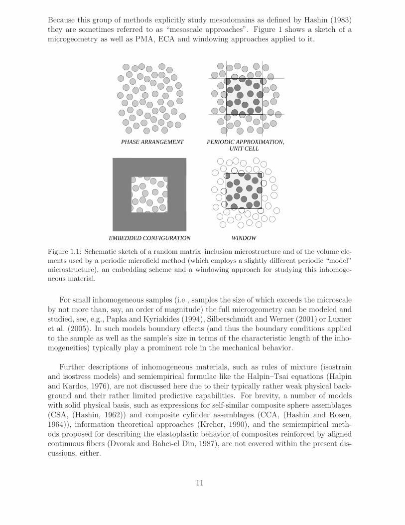
Because this group of methods explicitly study mesodomains as defined by Hashin (1983)they are sometimes referred to as “mesoscale approaches”. Figure 1 shows a sketch of amicrogeometry as well as PMA, ECA and windowing approaches applied to it.

PERIODIC APPROXIMATION,PHASE ARRANGEMENTUNIT CELL

EMBEDDED CONFIGURATION WINDOW

Figure 1.1: Schematic sketch of a random matrix–inclusion microstructure and of the volume ele-ments used by a periodic microfield method (which employs a slightly different periodic “model”microstructure), an embedding scheme and a windowing approach for studying this inhomoge-neous material.

For small inhomogeneous samples (i.e., samples the size of which exceeds the microscaleby not more than, say, an order of magnitude) the full microgeometry can be modeled andstudied, see, e.g., Papka and Kyriakides (1994), Silberschmidt and Werner (2001) or Luxneret al. (2005). In such models boundary effects (and thus the boundary conditions appliedto the sample as well as the sample’s size in terms of the characteristic length of the inho-mogeneities) typically play a prominent role in the mechanical behavior.

Further descriptions of inhomogeneous materials, such as rules of mixture (isostrainand isostress models) and semiempirical formulae like the Halpin–Tsai equations (Halpinand Kardos, 1976), are not discussed here due to their typically rather weak physical back-ground and their rather limited predictive capabilities. For brevity, a number of modelswith solid physical basis, such as expressions for self-similar composite sphere assemblages(CSA, (Hashin, 1962)) and composite cylinder assemblages (CCA, (Hashin and Rosen,1964)), information theoretical approaches (Kreher, 1990), and the semiempirical meth-ods proposed for describing the elastoplastic behavior of composites reinforced by alignedcontinuous fibers (Dvorak and Bahei-el Din, 1987), are not covered within the present dis-cussions, either.

11

For studying materials that are inhomogeneous at a number of (sufficiently widelyspread) length scales (e.g., materials in which well defined clusters of inhomogeneities arepresent), hierarchical procedures that use homogenization at more than one level are anatural extension of the above concepts. Such multi-scale models are the subject of a shortdiscussion in chapter 8.

12

Chapter 2

Mean Field Methods

In this chapter relations are given for two-phase materials only, extensions to multi-phasematerials being rather straightforward in most cases. Special emphasis is put on effectivefield methods of the Mori–Tanaka type, which may be viewed as the simplest mean fieldapproaches for modeling inhomogeneous materials that encompass the full physical rangeof phase volume fractions14. Unless specifically stated otherwise, the material behaviorof both reinforcements and matrix is taken to be linear (thermo)elastic. Perfect bondingbetween the constituents is assumed in all cases. There is an extensive body of literaturecovering mean field approaches, so that the following treatment is far from complete.

2.1 General Relations between Mean Fields in

Thermoelastic Two-Phase Materials

Throughout this report additive decomposition of strains is used. For example, for thecase of thermoelastoplastic material behavior the total strain tensor can be accordingly bewritten as

ε = εel + εpl + εth , (2.1)

where εel, εpl and εth denote the elastic, plastic and thermal strains, respectively. Strainand stress tensors can be split into volumetric and deviatoric contributions

ε = εvol + εdev = Qvol ε + Qdev ε

σ = σvol + σdev = Qvol σ + Qdev σ , (2.2)

Qvol and Qdev being the volumetric and deviatoric projection tensors.

For thermoelastic inhomogeneous materials, the macroscopic stress–strain relations canbe written in the form

〈σ〉 = E∗〈ε〉+ ϑ∗∆T

〈ε〉 = C∗〈σ〉+ α∗∆T . (2.3)

14Because Eshelby and Mori–Tanaka methods are specifically suited for matrix–inclusion-type micro-topologies, the expression “composite” is often used in the present chapter instead of the more generaldesignation “inhomogeneous material”.

13

Here the expression α∗∆T corresponds to the macroscopic thermal strain tensor, ϑ∗ =−E∗α∗ is the macroscopic specific thermal stress tensor (i.e., the overall stress responseof the fully constrained material to a purely thermal unit load), and ∆T stands for the(spatially homogeneous) temperature difference with respect to some stress-free referencetemperature. The constituents, here a matrix (m) and inhomogeneities (i), are also assumedto behave thermoelastically, so that

〈σ〉(m) = E(m)〈ε〉(m) + ϑ(m)∆T 〈σ〉(i) = E(i)〈ε〉(i) + ϑ(i)∆T

〈ε〉(m) = C(m)〈σ〉(m) + α(m)∆T 〈ε〉(i) = C(i)〈σ〉(i) + α(i)∆T , (2.4)

where the relations ϑ(m) = −E(m)α(m) and ϑ(i) = −E(i)α(i) hold.

From the definition of phase averaging, eqn. (1.13), the relations between the phaseaveraged fields,

〈ε〉 = ξ〈ε〉(i) + (1− ξ)〈ε〉(m) = εa

〈σ〉 = ξ〈σ〉(i) + (1− ξ)〈σ〉(m) = σa , (2.5)

where ξ = V (i) = Ω(i)/Ωs stands for the volume fraction of the reinforcements and 1− ξ =V (m) = Ω(m)/Ωs for the volume fraction of the matrix. εa and σa denote the far field(applied) homogeneous stress and strain tensors, respectively, with εa = C∗σa. Perfectinterfaces between the phases are assumed in expressing the macroscopic strain of the com-posite as the weighted sum of the phase averaged strains.

The phase averaged strains and stresses can be related to the overall strains and stressesby the phase strain and stress concentration tensors A, η, B, and β (Hill, 1963), respec-tively, which are defined for thermoelastic inhomogeneous materials by the expressions

〈ε〉(m) = A(m)〈ε〉+ η(m)∆T 〈ε〉(i) = A(i)〈ε〉+ η(i)∆T

〈σ〉(m) = B(m)〈σ〉+ β(m)

∆T 〈σ〉(i) = B(i)〈σ〉+ β(i)

∆T , (2.6)

compare eqn. (1.12) for the purely elastic case. A and B are referred to as the mechanicalor (elastic) phase stress and strain concentration tensors, respectively, and η as well as β

are the corresponding thermal concentration tensors.

By using eqns. (2.5) and (2.6), the strain and stress concentration tensors can be shownto fulfill the relations

ξA(i) + (1− ξ)A(m) = I ξη(i) + (1− ξ)η(m) = o

ξB(i) + (1− ξ)B(m) = I ξβ(i)

+ (1− ξ)β(m)

= o , (2.7)

where I stands for the symmetric rank 4 unit tensor and o for the rank 2 null tensor.

The effective elasticity and compliance tensors of the composite can be obtained fromthe properties of the phases and from the mechanical concentration tensors as

E∗ = ξE(i)A(i) + (1− ξ)E(m)A(m)

= E(m) + ξ[E(i) − E(m)]A(i) = E(i) + (1− ξ)[E(m) − E(i)]A(m) (2.8)

14

C∗ = ξC(i)B(i) + (1− ξ)C(m)B(m)

= C(m) + ξ[C(i) −C(m)]B(i) = C(i) + (1− ξ)[C(m) −C(i)]B(m) , (2.9)

compare eqn. (1.8). For multi-phase materials withN phases (p) the equivalents of eqn. (2.7)take the form

∑

(p)

A(p) = I∑

(p)

η(p) = o

∑

(p)

B(p) = I∑

(p)

β(p)

= o , (2.10)

and the effective elastic tensors can be evaluated as

E∗ =∑

(p)

ξ(p)E(p)A(p) C∗ =∑

(p)

ξ(p)C(p)B(p) (2.11)

in analogy to eqns. (2.8) and (2.9).The effective thermal expansion coefficient tensor, α∗, and the specific thermal stress

tensor, ϑ∗, can be related to the thermoelastic phase behaviors and the thermal concen-tration tensors as

α∗ = ξ[C(i)β(i)

+ α(i)] + (1− ξ)[C(m)β(m)

+ α(m)]

= ξα(i) + (1− ξ)α(m) + (1− ξ)[C(m) −C(i)]β(m)

= ξα(i) + (1− ξ)α(m) + ξ[C(i) −C(m)]β(i)

. (2.12)

ϑ∗ = ξ[E(i)η(i) + ϑ(i)] + (1− ξ)[E(m)η(m) + ϑ(m)]

= ξϑ(i) + (1− ξ)ϑ(m) + (1− ξ)[E(m) − E(i)]η(m)

= ξϑ(i) + (1− ξ)ϑ(m) + ξ[E(i) − E(m)]η(i) . (2.13)

The above expressions can be derived by inserting eqns. (2.4) and (2.6) into eqns. (2.5) andcomparing with eqns. (2.3). Alternatively, the overall coefficients of thermal expansion ofmulti-phase materials can be obtained as

α∗ =∑

(p)

ξ(p)(B(p))Tα(p) , (2.14)

compare (Mandel, 1965; Levin, 1967), an expression known as the Mandel–Levin formula.If the effective compliance tensor of a two-phase material is known eqn.(2.10) can beinserted into eqn.(2.14) to give the overall coefficients of thermal expansion as

α∗ = (C∗ −C(m))(C(i) −C(m))−1α(i) − (C∗ −C(i))(C(i) −C(m))−1α(m) . (2.15)

The mechanical stress and strain concentration tensors for a given phase are linked toeach other by expressions of the type

A(m) = C(m)B(m)E(i)[I + (1− ξ)(C(m) −C(i))B(m)E(i)]−1 = C(m)B(m)E∗

B(m) = E(m)A(m)C(i)[I + (1− ξ)(E(m) − E(i))A(m)C(i)]−1 = E(m)A(m)C∗ . (2.16)

15

In addition, by invoking the principle of virtual work relations were developed (Benvenisteand Dvorak, 1990; Benveniste et al., 1991) which link the thermal strain concentrationtensors, η(p), to the mechanical strain concentration tensors, A(p), and the thermal stress

concentration tensors, β(p)

, to the mechanical stress concentration tensors, B(p), respec-tively, as

η(m) = [I− A(m)][E(i) − E(m)]−1[ϑ(m) − ϑ(i)]

η(i) = [I− A(i)][E(m) − E(i)]−1[ϑ(i) − ϑ(m)]

β(m)

= [I− B(m)][C(i) −C(m)]−1[α(m) −α(i)]

β(i)

= [I− B(i)][C(m) −C(i)]−1[α(i) −α(m)] . (2.17)

From eqns. (2.9) to (2.17) it is evident that the knowledge of one elastic phase con-centration tensor is sufficient for describing the full thermoelastic behavior of a two-phaseinhomogeneous material within the mean field framework15. A fair number of additionalrelations between phase averaged tensors have been given in the literature which allow,e.g., the phase concentration tensors to be obtained from the overall and phase elastictensors.

2.2 Eshelby Tensor and Dilute Matrix–Inclusion

Composites

A large proportion of the mean field descriptions used in continuum micromechanics ofmaterials are based on the work of Eshelby (1957), who studied the stress and strain dis-tributions in homogeneous media that contain a subregion that spontaneously changes itsshape and/or size (undergoes a “transformation”) so that it no longer fits into its previ-ous space in the “parent medium”. Eshelby’s results show that if an elastic homogeneousellipsoidal inclusion (i.e., an inclusion consisting of the same material as the matrix) inan infinite matrix is subjected to a homogeneous strain εt (called the “stress-free strain”,“unconstrained strain”, “eigenstrain”, or “transformation strain”), the stress and strainstates in the constrained inclusion are uniform16, i.e., σ(i) = 〈σ〉(i) and ε(i) = 〈ε〉(i). Theuniform strain in the constrained inclusion (the “constrained strain”), εc, is related to thestress-free strain εt by the expression

εc = Sεt (2.18)

where S is referred to as the (interior point) Eshelby tensor. For eqn. (2.18) to hold, εt maybe any kind of eigenstrain that is uniform over the inclusion (e.g., a thermal strain or astrain due to some phase transformation which involves no changes in the elastic constantsof the inclusion).

15Similarly, n−1 elastic phase concentration tensors must be known for describing the overall thermoe-lastic behavior of an n-phase material.

16This “Eshelby property” or “Eshelby uniformity” is limited to ellipsoidal shapes (Lubarda and Marken-scoff, 1998). For certain nondilute periodic arrangements of inclusions, however, non-ellipsoidal shapes cangive rise to homogeneous fields (Liu et al., 2007).

16

For mean field descriptions of dilute matrix–inclusion composites, of course, the interestis focused on the stress and strain fields in inhomogeneous inclusions (“inhomogeneities”)that are embedded in a matrix. Such cases can be handled on the basis of Eshelby’stheory for homogeneous inclusions, eqn. (2.18), by introducing the concept of equivalenthomogeneous inclusions. This strategy involves replacing an actual perfectly bonded inho-mogeneous inclusion, which has different material properties than the matrix and which issubjected to a given unconstrained eigenstrain εt, with a (fictitious) “equivalent” homo-geneous inclusion on which a (fictitious) “equivalent” eigenstrain ετ is made to act. Thisequivalent eigenstrain must be chosen in such a way that the inhomogeneous inclusionand the equivalent homogeneous inclusion attain the same stress state σ(i) and the sameconstrained strain εc (Eshelby, 1957; Withers et al., 1989). When σ(i) is expressed in termsof the elastic strain in the inhomogeneity or inclusion, this condition translates into theequality

σ(i) = E(i)[εc − εt] = E(m)[εc − ετ ] . (2.19)

Here εc − εt and εc − ετ are the elastic strains in the inhomogeneity and the equivalenthomogeneous inclusion, respectively. Obviously, in the general case the stress-free strainswill be different for the equivalent inclusion and the real inhomogeneity, εt 6= ετ . Pluggingthe result of applying eqn. (2.18) to the equivalent eigenstrain, εc = Sετ , into eqn. (2.19)leads to the relationship

σ(i) = E(i)[Sετ − εt] = E(m)[S− I]ετ , (2.20)

which can be rearranged to obtain the equivalent eigenstrain as a function of the knownstress-free eigenstrain εt of the real inclusion as

ετ = [(E(i) −E(m))S + E(m)]−1E(i)εt . (2.21)

This, in turn, allows the stress in the inhomogeneity, σ(i), to be expressed as

σ(i) = E(m)(S− I)[(E(i) − E(m))S + E(m)]−1E(i)εt . (2.22)

The concept of the equivalent homogeneous inclusion can be extended to cases wherea uniform mechanical strain εa or external stress σa is applied to a perfectly bondedinhomogeneous elastic inclusion in an infinite matrix. Here, the strain in the inclusion, ε(i),is a superposition of the applied strain and of a term εc that accounts for the constrainteffects of the surrounding matrix. A fair number of different expressions for concentrationtensors obtained by such procedures have been reported in the literature, among the mosthandy being those proposed by Hill (1965b) and elaborated by Benveniste (1987). Forderiving them, the conditions of equal stresses and strains in the actual inclusion (elasticitytensor E(i)) and the equivalent inclusion (elasticity tensor E(m)) under an applied far fieldstrain εa take the form

σ(i) = E(i)[εa + εc] = E(m)[εa + εc − ετ ] (2.23)

andε(i) = εa + εc = εa + Sετ , (2.24)

respectively, where eqn. (2.18) is used to describe the constrained strain of the equivalenthomogeneous inclusion. On the basis of these relationships the strain in the inhomogeneitycan be expressed as

ε(i) = [I + SC(m)(E(i) −E(m))]−1εa . (2.25)

17

Because the strain in the inhomogeneity is homogeneous, ε(i) = 〈ε〉(i), the strain concen-tration tensor for dilute inhomogeneities follows directly as

A(i)dil = [I + SC(m)(E(i) −E(m))]−1 . (2.26)

By setting 〈ε〉(i) = C(i)〈σ〉(i) and using εa = C(m)σa, the dilute stress concentration tensorfor the inhomogeneities is found from eqn. (2.26) as

B(i)dil = E(i)[I + SC(m)(E(i) −E(m))]−1C(m)

= [I + E(m)(I− S)(C(i) −C(m))]−1 . (2.27)

Alternative expressions for dilute mechanical and thermal inclusion concentration tensorswere given, e.g., by Mura (1987), Wakashima et al. (1988) and Clyne and Withers (1993).All of the above relations were derived under the assumption that the inhomogeneities aredilutely dispersed in the matrix and thus do not “feel” any effects due to their neighbors(i.e., they are loaded by the unperturbed applied stress σa or applied strain εa, the socalled dilute case). Accordingly, the inclusion concentration tensors are independent of thereinforcement volume fraction ξ.

The stress and strain fields outside a transformed homogeneous or inhomogeneous in-clusion in an infinite matrix are not uniform on the microscale17 (Eshelby, 1959). Withinthe framework of mean field theories, which aim to link the average fields in matrix andinhomogeneities with the overall response of inhomogeneous materials, however, it is onlythe average matrix stresses and strains that are of interest. For dilute composites, suchexpressions follow directly by combining eqns. (2.26) and (2.27) with eqn. (2.7). Esti-mates for the overall elastic and thermal expansion tensors can, of course, be obtained ina straightforward way from the concentration tensors by using eqns. (2.8) to (2.17). Itmust be kept in mind, however, that the dilute expressions are strictly valid only for van-ishingly small inhomogeneity volume fractions and give dependable results only for ξ ≪ 0.1.

The Eshelby tensor S depends only on the material properties of the matrix and onthe aspect ratio a of the inclusions, i.e., expressions for the Eshelby tensor of ellipsoidalinhomogeneities are independent of the material symmetry and properties of the inhomo-geneities. Expressions for the Eshelby tensor of spheroidal inclusions in an isotropic matrixare given, e.g., by Pedersen (1983), Tandon and Weng (1984), Mura (1987) or Clyne andWithers (1993)18, the formulae being very simple for continuous fibers of circular cross-section (a→∞), spherical inclusions (a = 1), and thin circular disks (a→ 0). Closed formexpressions for the Eshelby tensor have also been reported for spheroidal inclusions in amatrix of transversely isotropic (Withers, 1989) or cubic material symmetry (Mura, 1987),provided the material axes of the matrix constituents are aligned with the orientations ofnon-spherical inclusions. In cases where no analytical solutions are available, the Eshelbytensor can be evaluated numerically, compare Gavazzi and Lagoudas (1990).

17The fields outside a single inclusion can be described via the (exterior point) Eshelby tensor, see, e.g.,Ju and Sun (1999). From the (constant) interior point fields and the (position) dependent exterior pointfields the stress and strain jumps at the interface between inclusion and matrix can be evaluated.

18Instead of evaluating the Eshelby tensor for a given configuration, the so called mean polarizationfactor tensor Q = E(m)(I− S) may be evaluated instead, see, e.g., Ponte Castaneda (1996).

18

2.3 Mean Field Methods for Thermoelastic

Composites with Aligned Reinforcements

Theoretical descriptions of the overall thermoelastic behavior of composites with reinforce-ment volume fractions of more than a few percent must explicitly account for interactionsbetween inhomogeneities, i.e., for the effects of all surrounding reinforcements on the stressand strain fields experienced by a given fiber or particle. Within the mean field frameworksuch interaction effects as well as the concomitant perturbations of the stress and strainfields in the matrix are accounted for in a collective way via suitable phase-wise constantapproximations. Beyond these “background effects”, there are interactions between indi-vidual reinforcements which, on the one hand, give rise to inhomogeneous stress and strainfields within each inhomogeneity (“intra-particle fluctuations”) and in the matrix. On theother hand, they cause the levels of the average stresses and strains in individual inhomo-geneities to differ (“inter-particle fluctuations”). These interactions and fluctuations arenot resolved by mean field methods.

Mori–Tanaka-Type Estimates

One way of introducing collective interactions between inhomogeneities consists of approx-imating the stresses acting on an inhomogeneity, which may be viewed as perturbationstresses caused by the presence of other inhomogeneities (“image stresses”, “backgroundstresses”) superimposed on the applied far field stress, by an appropriate average matrixstress. The idea of combining such a concept of an average matrix stress with Eshelby-type equivalent inclusion expressions goes back to Brown and Stobbs (1971) as well asMori and Tanaka (1973). Effective field theories of this type are generically referred to asMori–Tanaka methods. By construction they do not invoke explicit (e.g., pair-wise) inter-actions between “individual” inhomogeneities, but rather operate on a level of collectiveinteractions.

Benveniste (1987) pointed out that in the isothermal case the central assumption in-volved in Mori–Tanaka approaches can be denoted as

〈ε〉(i) = A(i)dil〈ε〉

(m)

〈σ〉(i) = B(i)dil〈σ〉

(m) . (2.28)

Thus, the methodology developed for dilute inhomogeneities is retained and the interac-tions with the surrounding inhomogeneities are accounted for by suitably modifying thestresses or strains acting on each inhomogeneity. Equation (2.28) may then be viewed as amodification of eqn. (1.12) in which the macroscopic strain or stress, 〈ε〉 or 〈σ〉, is replacedby the phase averaged matrix strain or stress, 〈ε〉(m) and 〈σ〉(m), respectively.

In a next step suitable expressions for 〈ε〉(m) and/or 〈σ〉(m) must be introduced into thescheme. This can be easily done by inserting eqn. (2.28) into eqn. (2.5), leading to theexpressions

〈ε〉(m) = [(1− ξ)I + ξA(i)dil]

−1〈ε〉

〈σ〉(m) = [(1− ξ)I + ξB(i)dil]

−1〈σ〉 . (2.29)

19

These, in turn, allow the Mori–Tanaka strain and stress concentration tensors for matrixand inhomogeneities to be written in terms of the dilute concentration tensors as

A(m)MT = [(1− ξ)I + ξA

(i)dil]

−1 A(i)MT = A

(i)dil[(1− ξ)I + ξA

(i)dil]

−1

B(m)MT = [(1− ξ)I + ξB

(i)dil]

−1 B(i)MT = B

(i)dil[(1− ξ)I + ξB

(i)dil]

−1 (2.30)

(Benveniste, 1987). Equations (2.30) may be evaluated with any strain and stress concen-

tration tensors A(i)dil and B

(i)dil pertaining to dilute inhomogeneities embedded in a matrix. If,

for example, the equivalent inclusion expressions, eqns. (2.26) and (2.27), are employed, theMori–Tanaka matrix strain and stress concentration tensors for the non-dilute compositetake the form

A(m)MT = (1− ξ)I + ξ[I + SC(m)(E(i) − E(m))]−1−1

B(m)MT = (1− ξ)I + ξE(i)[I + SC(m)(E(i) −E(m))]−1C(m) , (2.31)

compare Benveniste (1987), Benveniste and Dvorak (1990) or Benveniste et al. (1991).The Mori–Tanaka approximations to the effective elastic tensors are obtained by insertingeqns.(2.30) and/or (2.31) into eqns.(2.8) and (2.9).

A number of authors gave different but essentially equivalent Mori–Tanaka-type ex-pressions for the phase concentration tensors and effective thermoelastic tensors of inho-mogeneous materials, among them Pedersen (1983), Wakashima et al. (1988), Taya et al.(1991), Pedersen and Withers (1992) as well as Clyne and Withers (1993). Alternatively,the Mori–Tanaka method can be formulated to directly give the macroscopic elasticitytensor as

E∗T = E(m)

I− ξ[(E(i) − E(m))

(S− ξ(S− I)

)+ E(m)]−1[E(i) − E(m)]

−1(2.32)

(Tandon and Weng, 1984). Because eqn. (2.32) does not explicitly use the compliance ten-sor of the inhomogeneities, C(i), it can be modified in a straightforward way to describe themacroscopic stiffness of porous materials by setting E(i) → 0, giving rise to the relationship

ET,por = E(m)[I +

ξ

1− ξ(I− S)−1

]−1. (2.33)

which, however, should not be used for void volume fractions that are in excess of, say,ξ = 0.2519.

As is evident from their derivation, Mori–Tanaka-type theories at all volume fractionsdescribe composites consisting of aligned ellipsoidal inhomogeneities embedded in a matrix,i.e., inhomogeneous materials with a distinct matrix–inclusion microtopology. More pre-cisely, it was shown by Ponte Castaneda and Willis (1995) that Mori–Tanaka methods area special case of Hashin–Shtrikman variational estimates (compare section 2.4) in which

19Mori–Tanaka theories are based on the assumption that the shape of the inhomogeneities can bedescribed by ellipsoids of a given aspect ratio throughout the deformation history. In porous materialswith high void volume fractions deformation at the microscale takes place mainly by bending and bucklingcell walls or struts (Gibson and Ashby, 1988), which implies changes of the shapes of the voids. Sucheffects are not described by Mori–Tanaka models, which, consequently, tend to overestimate the effectivestiffness of cellular materials by far.

20

the spatial arrangement of the inhomogeneities follows an aligned ellipsoidal distribution,which is characterized by the same aspect ratio as the shape of the inhomogeneities them-selves, compare fig. 2.1.

Figure 2.1: Sketch of ellipsoidal inhomogeneities in an aligned ellipsoidally distributed spatialarrangement as used implicitly in Mori–Tanaka-type approaches (a=2.0).

For two-phase composites Mori–Tanaka estimates coincide with Hashin–Shtrikman-type bounds (compare section 3.1) and, accordingly, their predictions for the overallYoung’s and shear moduli are always on the low side for composites reinforced by alignedor spherical reinforcements that are stiffer than the matrix (see the comparisons in section3.4 as well as tables 5.1 to 5.3) and on the high side for materials containing compliantreinforcements in a stiffer matrix. In high contrast situations they tend to under- or over-estimate the effective elastic properties by a considerable margin, compare table 5.3. Fordiscussions of further issues with respect to the range of validity of Mori–Tanaka theoriesfor elastic inhomogeneous two-phase materials see Christensen et al. (1992).

For multi-phase materials consisting of a matrix (m) into which N − 1 inhomogeneityphases are embedded the Mori–Tanaka phase concentration tensors take the form

A(m)MT =

[ξ(m)I +

∑(j)6=(m)

ξ(j)A(j)dil

]−1A

(i)MT = A

(i)dil

[ξ(m)I +

∑

(j) 6=(m)

ξ(j)A(j)dil

]−1

B(m)MT =

[ξ(m)I +

∑(j)6=(m)

ξ(j)B(j)dil

]−1B

(i)MT = A

(i)dil

[ξ(m)I +

∑

(j) 6=(m)

ξ(j)B(j)dil

]−1(2.34)

and the macroscopic elastic tensors are obtained as

E∗MT =

[ξ(m)E(m) +

∑

(i)6=(m)

ξ(i)E(i)A(i)dil

] [ξ(m)I +

∑

(i) 6=(m)

ξ(i)A(i)dil

]−1

C∗MT =

[ξ(m)C(m) +

∑

(i) 6=(m)

ξ(i)C(i)B(i)dil

] [ξ(m)I +

∑

(i) 6=(m)

ξ(i)B(i)dil

]−1

. (2.35)

These expressions are rigorous bounds only if the matrix is the most compliant or thestiffest constituent.

21

Mori–Tanaka-type theories can be implemented into computer programs in a straight-forward way. Because they are explicit algorithms, all that is required are matrix additions,multiplications, and inversions plus expressions for the Eshelby tensor. Despite their limita-tions, Mori–Tanaka approaches provide useful accuracy for the elastic contrasts pertainingto most practically relevant composites. This combination of features makes them impor-tant tools for evaluating the stiffness and thermal expansion properties of inhomogeneousmaterials that show a matrix–inclusion topology with aligned inhomogeneities or voids.Mori–Tanaka-type approaches for thermoelastoplastic materials are discussed in section2.4 and “extended” Mori–Tanaka approaches for nonaligned reinforcements in section 2.7.

Classical Self-Consistent Estimates

Another group of estimates for the overall thermomechanical behavior of inhomogeneousmaterials are effective medium theories, in which an inhomogeneity or some phase arrange-ment, the kernel, is embedded in the effective material (the properties of which are notknown a priori). Figure 2.2 shows a schematic comparison of the material and loadingconfigurations underlying Eshelby models, effective field (Mori–Tanaka) methods and twoeffective medium approaches, the classical self-consistent and generalized self-consistent(compare section 2.4) schemes20.

effeffmmm

i i i i

σ σ σσa tot a a(m)

GSCSCSCSMTMdiluteFigure 2.2: Schematic comparison of the Eshelby method for dilute composites, Mori–Tanakaapproaches and classical as well as generalized self-consistent schemes.

If the kernel consists of a dilute inhomogeneity, classical (or two-phase) self-consistentschemes are obtained (CSCS), see, e.g., Hill (1965b). They are based on rewriting eqn. (2.26)and (2.27) for an inhomogeneity that is surrounded by the effective medium instead of

the matrix, i.e., E(m) → E∗ and C(m) → C∗, so that A(i)dil → A

(i)dil(E

∗,C∗) and B(i)dil →

B(i)dil(E

∗,C∗). The results of the above formal procedure can be inserted into eqn. (2.8),giving rise to the relationships

E∗SCS = E(m) + ξ[E(i) −E(m)] A

(i)dil(E

∗,C∗)

= E(m) + ξ[E(i) −E(m)] [I + SC(E(i) −E∗SCS)]

−1

C∗SCS = C(m) + ξ[C(i) −C(m)] B

(i)dil(E

∗,C∗)

= C(m) + ξ[C(i) −C(m)] [I + E∗(I− S)(C(i) −C∗SCS)]

−1 , (2.36)

20Within the classification of micromechanical methods given in section 1.5, self-consistent mean fieldmethods can also be viewed as as analytical embedding approaches.

22

where S has to be evaluated with respect to the effective material. Equations (2.36) canbe interpreted as an implicit nonlinear system of equations for the unknown elastic tensorsE∗ = E∗

SCS and C∗ = C∗SCS, which describe the behavior of the effective medium. This

system can be solved by self-consistent iterative schemes of the type

En+1 = E(m) + ξ[E(i) −E(m)][I + SnCn(E(i) − En)]

−1

Cn+1 =[En+1

]−1. (2.37)

The Eshelby tensor Sn in eqn. (2.37) describes the response of an inhomogeneity embed-ded in the n-th iteration of the effective medium; it must be recomputed for each iteration21.

For multi-phase composites the classical self-consistent estimate for the effective elas-ticity tensor takes the form

E∗SC,n =

∑

(p)

E(p)I + S

(p)n−1CSC,n−1[E

(p) − ESC,n−1]−1

C∗SC,n = (E∗

SC,n)−1 , (2.38)

where S(p)n−1 pertains to an ellipsoidal inhomogeneity with the shape of phase (p).

The predictions of the CSCS differ noticeably from those of Mori–Tanaka methods inbeing close to the Hashin–Shtrikman lower bounds (see section 4) for low reinforcementvolume fractions, but close to the upper bounds for reinforcement volume fractions ap-proaching unity (compare figs. 3.1 to 3.7). Generally, two-phase self-consistent schemesare best suited to describing the overall properties of two-phase materials that do notshow a matrix–inclusion microtopology at some or all of the volume fractions of interest22.Essentially, the microstructures described by two-phase CSCS are characterized by inter-penetrating phases around ξ = 0.5, with one of the materials acting as the matrix forξ → 0 and the other for ξ → 1. Consequently, the CSCS is typically not the best choice fordescribing composites showing a matrix–inclusion topology, but is well suited to studyingFunctionally Graded Materials (FGMs) in which the volume fraction of a constituent canvary from 0 to 1 through the thickness of a sample. Multi-phase versions of the CSCS,such as eqn.(2.38) are important methods for modeling polycrystals. When microgeome-tries described by the CSCS show a geometrical anisotropy, this anisotropy determines theshapes or aspect ratios of the “inhomogeneity” used in the model.

For porous materials classical self-consistent schemes predict a breakdown of the stiff-ness due to the percolation of the pores at ξ = 1

2for spherical voids and at ξ = 1

3for

aligned cylindrical voids (Torquato, 2002).

Because self-consistent schemes are by definition implicit methods, their computationalrequirements are in general higher than those of Mori–Tanaka-type approaches. Like ef-

21For aligned spheroidal but non-spherical inhomogeneities the effective medium shows transverselyisotropic behavior, so that an appropriate evaluation procedure for evaluating the Eshelby tensor must beused.

22Classical self-consistent schemes can be shown to correspond to perfectly disordered materials (Kroner,1978) or self-similar hierarchical materials (Torquato, 2002). Note that in contrast to eqn. (2.11), in theCSCS expression, eqn. (2.38), all phases are treated on an equal footing.

23

fective field models, they can form the basis for describing the behavior of nonlinear inho-mogeneous materials.

Differential Schemes

A further important group of mean field approaches are differential schemes (McLaughlin,1977; Norris, 1985), which may be envisaged as involving repeated cycles of adding smallconcentrations of inhomogeneities to a material and then homogenizing. Following Hashin(1988) the overall elastic tensors can accordingly be described by the differential equations

dE∗D

dξ=

1

1− ξ[E(i) −E∗

D]Adil(E∗D)

dC∗D

dξ=

1

1− ξ[C(i) −C∗

D]Bdil(E∗D) (2.39)

with the initial conditions E∗D=E(m) and C∗

D=C(m), respectively, at ξ=0. In analogy toeqn. (2.36) Adil and Bdil depend on E∗

D and C∗D, respectively. Equations (2.39) can be in-

tegrated with standard numerical algorithms for initial value problems, e.g., Runge–Kuttaschemes.

Differential schemes can be related to matrix–inclusion microgeometries with poly-disperse distributions of the sizes of the inhomogeneities (corresponding to the repeatedhomogenization steps) 23. Because of their association with specific microgeometries thatare not typical of “classical composites” (in which reinforcement size distributions usuallyare not very wide24) and due to their higher mathematical complexity (as compared, e.g.,to Mori–Tanaka models) Differential Schemes have seen limited use in studying the me-chanical behavior of composite materials.

2.4 Hashin–Shtrikman Estimates

The stress field in an inhomogeneous material can be expressed in terms of a homogeneouscomparison (or reference) medium having an elasticity tensor E0 as

σ(x) = E(x) ε(x) = E0 ε(x) + τ 0(x) . (2.40)

where τ 0(x) = (E(x)− E0) ε(x) is known as the polarization tensor. Phase averaging ofτ 0(x) over phase (p) leads to the phase averaged polarization tensor

〈τ 0〉(p) = [E(p) − E0]〈ε〉(p) = 〈σ〉(p) −E0〈ε〉(p) , (2.41)

23The interpretation of differential schemes of involving the repeated addition of infinitesimal volumefractions of inhomogeneities of increasingly larger size, followed each time by homogenization, is due toRoscoe (1973). It was pointed out, however, by Hashin (1988) that the requirements of infinitesimal volumefraction and growing size of the inhomogeneities may lead to contradictions.

24However, with the exception of the CSCS for two-dimensional conduction (Torquato and Hyun, 2001),none of the mean field methods discussed in section 2.3 corresponds to a realization in the form of amonodisperse matrix–inclusion microgeometry.

24

which can be directly used in a mean field framework.

Equation (2.41) can be used as the starting point for deriving general mean field strainconcentration tensors in dependence on the elasticity tensor of a reference materials. Fol-lowing Bornert (2001) these concentration tensors take the form

A(m)HS = [L0 + E(m)]−1

[ξ(L0 + E(i))−1 + (1− ξ)(L0 + E(m))−1

]−1

A(i)HS = [L0 + E(i)]−1

[ξ(L0 + E(i))−1 + (1− ξ)(L0 + E(m))−1

]−1, (2.42)

where the tensor L0, which is known as the overall constraint tensor (Hill, 1965b) or Hill’sinfluence tensor, is defined as

L0 = E0[(S0)−1 − I] . (2.43)

The Eshelby tensor S0 has to be evaluated with respect to the comparison material. Equa-tions (2.42) lead to estimates for the overall elastic stiffness of two-phase materials in theform

E∗HS = E(m) + ξ(E(i) − E(m))

[I + (1− ξ)(L0 + E(m))−1(E(i) −E(m))

]−1, (2.44)

which are referred to as Hashin–Shtrikman elastic tensors (Bornert, 2001).

Standard mean field models can be obtained as special cases of Hashin–Shtrikmanmethods by appropriate choices of the comparison material. For example, using the matrixas the comparison material results in Mori–Tanaka methods, whereas the selection of theeffective material as comparison material leads to classical self-consistent schemes.

Generalized Self-Consistent Estimates

The above Hashin–Shtrikman formalism can be extended in a number of ways, one of whichconsists in not only studying inhomogeneities but also more complex geometrical entities,called patterns or motifs, embedded in a matrix, see Bornert (1996) and Bornert (2001).Typically the stress and strain fields in such patterns are inhomogeneous even in the di-lute case and numerical methods must be used for evaluating the corresponding overallconstraint tensors. The simplest example of such a pattern consists of a spherical particleor cylindrical fiber surrounded by a constant-thickness layer of matrix at an appropriatevolume fraction, which, when embedded in the effective material, allows to recover thethree-phase or generalized self-consistent scheme (GSCS) of Christensen and Lo (1979),compare fig. 2.2 and see also (Christensen and Lo, 1986). GSCS expressions for the overallelastic moduli can also be obtained by considering the differential equations describingthe elastic response of such three-phase regions under appropriate boundary and loadingconditions. The GSCS in its original version is limited to inhomogeneities of spherical orcylindrical shape, where it is closely related but not identical to microgeometries of theCSA and CCA types (Christensen, 1998), respectively. It gives rise to third-order equa-tions for the shear modulus G and the transverse shear modulus GT, and its results for thebulk and transverse bulk moduli coincide with those obtained from the CSA and CCA,respectively. Extensions of the GSCS to multi-layered spherical inhomogeneities (Herveand Zaoui, 1993) and to aligned ellipsoidal inhomogeneities (Huang and Hu, 1995) were

25

also reported in the literature.

Generalized self-consistent schemes give excellent results for inhomogeneous materialswith matrix–inclusion topologies and are accordingly highly suited for obtaining estimatesfor the thermoelastic moduli of composite materials reinforced by spherical or equiaxedparticles or aligned continuous fibers. They are, however, not mean-field schemes in thesense of section 2.3.

2.5 Other Analytical Estimates for Elastic

Composites with Aligned Reinforcements

Interpolative schemes can be constructed that generate estimates between mean-field mod-els describing, on the one hand, some composite and, on the other hand, a material in whichthe roles of matrix and reinforcements are interchanged (referred to, e.g., as Mori–Tanakaand Inverse Mori–Tanaka schemes), see, e.g., Lielens et al. (1997). Such approaches, whilebeing capable of providing useful estimates for given composites, have the drawback oftypically not being associated with realizable microgeometries.

Ponte Castaneda and Willis (1995) proposed a refined mean field scheme for inhomo-geneous materials that consist of ellipsoidal arrangements of ellipsoidal inhomogeneitiesembedded in a matrix. In such systems the spatial correlations of the inhomogeneityarrangement can be described by an Eshelby tensor Sd, whereas the shapes of the inhomo-geneities are introduced via the Eshelby tensor Si. The corresponding phase arrangementscan be visualized by extending fig. 2.1 to non-overlapping “safety ellipsoids” that containaligned or non-aligned ellipsoidal inhomogeneities, the aspect ratios of the safety ellipsoidsand the inhomogeneities being different. The inclusion strain concentration tensors of suchmicrogeometries can be expressed as

A(i)PW =

[I + (Si − ξSd)C

(m)(E(i) −E(m))]−1

=[(E(i) −E(m))−1 − ξA

(i)dil SdC

(m)]−1

, (2.45)

from which the macroscopic elasticity tensor follows as

E∗PW = E(m) + ξ[E(i) −E(m)]

[I + (Si − ξSd)C

(m)(E(i) − E(m))]−1

= E(m) + ξ[(E(i) − E(m))−1 − ξA

(i)dil SdC

(m)]−1

A(i)dil (2.46)

via eqn.(2.8). This model is known as the Hashin–Shtrikman estimates of Ponte Castanedaand Willis (1995) and it is strictly valid as long as the inhomogeneities do not penetratetheir respective safety ellipsoids. When both the inhomogeneities and the safety ellipsoidsare aligned and Si = Sd, eqn. (2.46) becomes equivalent to the corresponding Mori–Tanakaexpression, which shows that Mori–Tanaka methods are a special case of the Hashin–Shtrikman estimates. For a discussion of the latters’ relationship to other micromechanicalschemes see Hu and Weng (2000). For multi-phase composites the Ponte–Willis estimatesfor the elasticity tensor take the form

E∗PW = E(m) +

∑

(i) 6=(m)

ξ(i)[I−

∑

(j) 6=(m)

ξ(j)(E(j) − E(m))A(j)dil S

(i)d C(m)

]−1

(E(j) −E(m))A(i)dil (2.47)

26

and the strain concentration tensor for inhomogeneity (i) is

A(i)PW = A

(i)dil

[I−

∑

(j) 6=(m)

ξ(j)S(i)d C(m)(E(j) − E(m))A

(j)dil

]. (2.48)

Here S(i)d describes the “safety ellipsoids” pertaining to phase (i). Analogous results can

be obtained with the Interaction Direct Derivative (IDD) approach of Du and Zheng (2002).

An important group of analytical models for the macroscopic elastic response of inho-mogeneous materials are estimates based on n-point statistics, which are not mean fieldapproaches in the sense of most other methods discussed in chapter 2. Three-point esti-mates for the thermoelastic properties of two-phase materials were developed by Torquato(1998) and use the same pair of three-point microstructural parameters, η and ζ , employedby the three-point bounds discussed in section 3.2. These estimates lie between the cor-responding bounds and give excellent analytical predictions for the overall thermoelasticresponse of inhomogeneous materials that show the appropriate microgeometries and arefree of flaws. For discussion of further estimates for the overall elastic properties of inho-mogeneous materials see, e.g., Torquato (2002).

2.6 Mean Field Methods for Inelastic Composites

Over the past two decades considerable efforts have been directed at modeling the me-chanical behavior of inhomogeneous materials in which one or more constituents showviscoelastic, elastoplastic or viscoelastoplastic responses. The main motivation of suchstudies has been need to describe the time dependent behavior of polymer matrix compos-ites and the responses of composites with metallic phases. Mean field methods have beendeveloped for and successfully adapted to studying many aspects of such problems.

If the behavior of an inhomogeneous material is not only inelastic, but also nonlinear,suitable linearization schemes are required, which reduce the nonlinear problem to a se-quence of linear ones. In continuum micromechanics, the most important approaches ofthis type this are secant (Tandon and Weng, 1988) and incremental (Hill, 1965a) meth-ods. In addition, tangent concepts (Molinari et al., 1987) and, recently, affine formulations(Masson et al., 2000; Brenner et al., 2001) have been reported.

Viscoelastic Composites

Viscoelastic materials show hereditary behavior, i.e., their response at a given time dependson their previous load history. Important issues in the mechanical behavior of viscoelas-tic composites are, on the one hand, quasi-static responses such as relaxation and creep,which can be described via relaxation relaxation function and creep compliance tensors.The dynamic behavior under periodic excitations, on the other hand, can be studied viacomplex modulus tensors.

Correspondence principles are available (Hashin, 1965, 1970) that directly relate theanalysis of linear viscoelastic composites to that of elastic composites of identical phase ge-

27

ometry of both of the above sets of problems, see also Schapery (1974) and Hashin (1983).For the quasi-static case the correspondence principle requires formulating the quasi-staticviscoelastic problem in the Carson–Laplace transformed domain, where expressions for thetransformed relaxation function and creep compliance tensors are equivalent to estimatesfor the elasticity and compliance tensors, respectively, in elastic micromechanics. On thisbasis replacement schemes can be defined (Hashin, 1972) that allow to obtain Laplacetransformed macroscopic moduli, modulus tensors and phase averaged microfields of vis-coelastic materials from mean field results such as the ones discussed in sections 2.3 to 2.5.The back transformation from the Carson–Laplace to the time domain, however, typicallyis not straightforward and does not provide closed form solutions in most cases, approxima-tions having to be introduced or numerical methods to be used, compare Schapery (1962)and Levesque et al. (2007). The correspondence principle for periodic excitations usestransforms to Fourier space and the resulting replacement scheme (Hashin, 1972) directlygenerates effective complex modulus tensors from the effective elastic tensors obtained fora given microgeometry25.

For in-depth discussions of and alternative concepts for mean field models of linearand nonlinear viscoelastic composites see, e.g., Paquin et al. (1999), Brenner and Masson(2005), Levesque et al. (2007), as well as Lahellec and Suquet (2007).

(Thermo)Elastoplastic Composites

The following discussion is restricted to mean field models based on continuum plasticity26.Nearly all work reported on such models for elastoplastic or viscoelastoplastic inhomoge-neous materials has relied on secant, incremental, tangent or affine linearization strategies.A fairly recent overview of mean field methods for elastoplastic composites was given byPonte Castaneda and Suquet (1998).

The main difficulties in applying mean field methods to composites with elastoplasticconstituents lie in the path dependence of plastic behavior and in the typically strong intra-phase fluctuations of the microstress and microstrain fields in elastoplastic inhomogeneousmaterials. Accordingly, each material point in an elastoplastic phase tends to follow a dif-ferent trajectory in stress space, so that even a two-phase elastoplastic composite effectivelybehaves as a multi-phase material and phase averages over matrix and reinforcements areless useful descriptors than in the linear elastic case. As a consequence, in mean field mod-els of elastoplastic composites choices have to be made with respect to the linearizationprocedure, the linear homogenization model, and the phase-wise equivalent stresses andequivalent strains to be used in evaluating the elastoplastic constituent material behavior(Zaoui, 2001).

25The correspondence principles can be applied, on the one hand, to analytical expressions, such as theCSA and CCA models (Hashin, 1972), and on the other hand, to numerical results obtained with theDiscrete Microfield Approaches discussed in chapters 5 to 7, see, e.g., Brinson and Lin (1998) or Yi et al.(1998).

26In a separate line of development, phase averaged stress fields obtained by Eshelby-based methodshave been used in dislocation-based descriptions of elastoplastic matrix behavior, see, e.g., Taya and Mori(1987).

28

Secant Methods for Elastoplastic Composites

Secant plasticity concepts in continuum micromechanics, see, e.g., Tandon and Weng (1988)or Dunn and Ledbetter (1997), are based on the deformation theory of plasticity, in whichelastoplastic behavior is approximated by nonlinear elastic models.

In the simplest case of an isotropic elastoplastic phase that is described by J2 plasticity,the secant “elastic” and “compliance” tensors, E

(p)sec and C

(p)sec, take the form

E(p)sec = 3K(p)QE

vol + 2G(p)secQ

Edev and C(p)

sec =1

3K(p)QC

vol +1

2G(p)sec

QCdev , (2.49)

respectively. Here QE and QC are the volumetric and deviatoric “partitioning tensors” forelasticities and compliances27, respectively. The secant shear modulus G

(p)sec is equal to the

elastic shear modulus of the matrix, G(p), in the elastic range. In the post-yield regime itcan be obtained from the current phase averages of the equivalent stress 〈σeqv〉

(p) and theequivalent plastic strain 〈εeqv,pl〉

(p) as

G(p)sec =

G(p) 〈σeqv〉(p)

〈σeqv〉(p) + 3G(p)〈εeqv,pl〉(p)(2.50)

on the basis of an additive strain decomposition, compare eqn. (2.1). εeqv,pl must be eval-uated from σeqv via an appropriate hardening law.

Expressions for the macroscopic secant tensors E∗sec and C∗

sec can be obtained from thephase secant tensors, eqn. (2.49), by mean field relationships equivalent to eqns. (2.8) and(2.9). For the case of elastic inhomogeneities embedded in an elastoplastic matrix thesetake the form

E∗sec = E(m)

sec + ξ(E(i) − E(m)sec)A

(m)sec

C∗sec = C(m)

sec + ξ(C(i) −C(m)sec)B

(m)sec . (2.51)

The non-dilute secant strain and stress concentration tensors, A(m)sec and B

(m)sec, can be gener-

ated from dilute secant concentration tensors, A(m)dil,sec and B

(m)dil,sec, via a suitable mean field

theory, e.g., a Mori–Tanaka method or a self-consistent scheme, compare section 2.3. Thedilute secant concentration tensors and the Eshelby tensors contained in them, in turn,must be evaluated using the current secant tensors of the constituents. Iterative proce-dures are required for obtaining solutions corresponding to prescribed macroscopic strainor stress states.

In first order methods, the phase average of the equivalent stress required in eqn. (2.50)is approximated from the phase averaged stress tensor,

〈σeqv〉(p) ≈

[3

2〈σ〉Tdev〈σ〉dev

] 12

, (2.52)

27In index notation the QE and QC are equal to each other and to the volumetric and deviatoricprojection tensors Q defined in eqn. (2.2). The use of shear angles in the present engineering notation,however, leads to differences in the shear terms of QE

dev, QCdev and Qdev.

29

which neglects contributions from the local stress fluctuations and, accordingly, tends tounderestimate 〈σeqv〉

(p), leading to underestimates of the macroscopic effective stress28. Im-proved results can be obtained by second order approximations that obtain the phase

averaged equivalent stress in terms of the second order moments of stress,⟨σ ⊗ σ

⟩(p),

(Suquet, 1995; Buryachenko, 1996; Hu, 1997; Ju and Sun, 2001) or on the basis of energyconsiderations (Qiu and Weng, 1992).

Alternatively, secant theories for composites with nonlinear constituents can be ob-tained from variational principles (Ponte Castaneda, 1991) or they can be formulated interms of potentials (Bornert and Suquet, 2001), which allows for a concise mathematicalpresentation. Because secant models treat elastoplastic composites as nonlinearly elasticmaterials they are limited to strictly monotonic loading and to radial (or approximatelyradial) trajectories of the phase averaged stresses of the constituents in stress space29,which precludes their use as micromechanically based constitutive models or as lower scalemodels in multi-scale analysis.

“Modified secant models” (Ponte Castaneda and Suquet, 1998) that use second orderapproximations for 〈σeqv〉

(p), however, have been found to be highly suitable for materialscharacterization of elastoplastic composites, where they have shown excellent agreementwith predictions from multi-particle unit cell models (Segurado et al., 2002a) and exper-iments. Modified secant models have also proved quite flexible. For example, method ofthis type was adapted to incorporate a nonlocal plasticity model for the matrix (Hu et al.,2005) in order to study particle size effects on the macroscopic yield behavior of particlereinforced MMCs.

Incremental Methods for Elastoplastic Composites

Incremental mean field methods can be formulated on the basis of strain and stress ratetensors for elastoplastic phases (p), d〈ε〉(p) and d〈σ〉(p), which can be expressed in analogyto eqn. (2.6) as

d〈ε〉(p) = A(p)t d〈ε〉+ η

(p)t dT

d〈σ〉(p) = B(p)t d〈σ〉+ β

(p)t dT , (2.53)

where d〈ε〉 stands for the macroscopic strain rate tensor, d〈σ〉 for the macroscopic stress

rate tensor, and dT for a homogeneous temperature rate. A(p)t , η

(p)t , B

(p)t , and β

(p)t are

instantaneous strain and stress concentration tensors, respectively. Assuming the inho-mogeneities to show elastic and the matrix to show elastoplastic material behavior30, the

28As an extreme case, using eqn. (2.52) for evaluating the equivalent stress leads to predictions that mate-rials with spherical reinforcements will not yield under macroscopically hydrostatic loads or unconstrainedthermal expansion. This is in contradiction to experimental and other theoretical results.

29The condition of radial loading paths in stress space at the constituent level is generally violated by aconsiderable margin in the phases of elastoplastic inhomogeneous materials, even for macroscopic loadingpaths that are perfectly radial (Pettermann, 1997). This behavior is due to changes in the accommodationof the phase stresses and strains in inhomogeneous materials upon yielding of a constituent and, to a muchlesser extent, in the strain hardening regime.

30Analogous expressions can be derived for elastoplastic inhomogeneities in an elastic matrix or, ingeneral, for composites containing any required number of elastoplastic phases.

30

overall instantaneous (tangent) stiffness tensor can be written in terms of the phase prop-erties and the instantaneous concentration tensors as

E∗t = E(i) + (1− ξ)[E

(m)t −E(i)]A

(m)t

= [C(i) + (1− ξ)[C(m)t −C(i)]B

(m)t ]−1 , (2.54)

compare eqns. (2.8) and (2.9).

Using the Mori–Tanaka formalism of Benveniste (1987), the instantaneous matrix con-centration tensors take the form

A(m)t = (1− ξ)I + ξ[I + StC

(m)t (E(i) − E

(m)t )]−1−1

B(m)t = (1− ξ)I + ξE(i)[I + StC

(m)t (E(i) −E

(m)t )]−1C

(m)t

−1 , (2.55)

compare eqn. (2.31). Expressions for the instantaneous thermal concentration tensors andinstantaneous coefficients of thermal expansion can be derived in analogy to the corre-sponding thermoelastic relations, e.g., eqns. (2.13) and (2.17). Equations (2.55) use theinstantaneous Eshelby tensor St, which depends on the current state of the (elastoplastic)

matrix material, E(m)t , and, in general, has to be evaluated numerically.

By replacing rates such as d〈σ〉(p) with finite increments such as ∆〈σ〉(p) formulationsof eqns. (2.53) to (2.55) can be obtained that are suitable for implementation as microme-chanically based constitutive models at the integration point level within Finite Elementcodes. The resulting incremental Mori–Tanaka (IMT) methods make no assumptions onthe overall yield surface and the overall flow potential, the effective material behaviorbeing entirely determined by the incremental mean field equations and the constitutivebehavior of the phases. As a consequence, mapping of the stresses onto the yield surfacecannot be handled at the level of the homogenized material and radial return mappingmust be applied to the matrix at the microscale instead. This implies that the constitutiveequations describing the overall behavior cannot be integrated directly (as is the case forhomogeneous elastoplastic materials), and iterative algorithms are required. For example,Pettermann (1997) used an implicit Euler scheme in an implementation of an incrementalMori–Tanaka method as a user supplied material routine (UMAT) for the Finite Elementcode ABAQUS (Simulia, Pawtucket, RI). Extended versions of such algorithms can alsohandle thermal expansion effects31 and temperature dependent material parameters.

Incremental mean field models of the type discussed above tend to overestimate themacroscopic strain hardening in the post-yield regime to such an extent that their prac-tical applicability is rather limited, especially for matrix dominated deformation modes,compare, e.g., the discussions by Gilormini (1995) and Suquet (1997). Recent developmentsinvolve the use of tangent operators that reflect the macroscopic symmetry of the com-posite, e.g., “isotropized” operators32 for statistically isotropic materials (Bornert, 2001),

31Elastoplastic inhomogeneous materials such as metal matrix composites typically show a hystereticthermal expansion response, i.e., the “coefficients of thermal expansion” are not material properties in thestrict sense. This dependence of the thermal expansion behavior on the instantaneous mechanical responserequires special treatment within the IMT framework, compare Pettermann (1997).

32For a discussion of a number of issues pertaining to the use of “isotropic” versus “anisotropic” tangentoperators see, e.g., Chaboche and Kanoute (2003).

31

and algorithmic modifications (Doghri and Ouaar, 2003; Doghri and Friebel, 2005). Theseimprovements have succeeded in markedly reducing the above weaknesses of incrementalmean field models such as incremental Mori–Tanaka methods for particle reinforced com-posites, rendering them highly useful for practical applications and making them attractivecandidates for use at the lower length scale in multi-scale models of ductile matrix compos-ites, compare chapter 8. IMTs were also successfully extended to the large strain regime(Huber et al., 2007).

Incremental mean field models have typically used eqn. (2.52) for evaluating the phaseaveraged equivalent stresses, which, accordingly, tend to be underestimated. The improvedestimators for 〈σeqv〉

(p) used in modified secant models are not suitable for incrementalmethods, for which an empirical correction was proposed by Delannay et al. (2007). Fur-thermore, because they assume elastoplastic phases to yield as a whole once the phaseaveraged equivalent stress exceeds the yield stress of the elastoplastic constituent, meanfield approaches predict sharp transitions from elastic to plastic states instead of a morerealistic gradual progress of yielded regions at the microscale.

Other mean field schemes can also be combined with secant and incremental approachesto obtain descriptions for elastoplastic inhomogeneous materials, the most important appli-cation having been the use of classical self-consistent schemes for describing the elastoplas-tic behavior of polycrystalline materials, see, e.g., (Hill, 1965a; Hutchinson, 1970; Berveillerand Zaoui, 1981). In the case of incremental methods what has to be done is replacingelastic, Eshelby and concentration tensors with the corresponding instantaneous tensorsfor each elastoplastic phase in expressions such as eqns. (2.36), (2.38), (2.46) or (2.47). Theweaknesses and strengths of such procedures are closely related to those discussed abovefor the Mori–Tanaka method. In addition, mean field approaches have been employed toobtain estimates for the nonlinear response of inhomogeneous materials due to microscopicdamage or to combinations of damage and plasticity, see, e.g., (Tohgo and Chou, 1996;Guo et al., 1997).

As an alternative to directly extending mean field theories into secant or incrementalplasticity, they can also be combined with Dvorak’s Transformation Field Analysis (Dvorak,1992) in order to obtain descriptions of the overall behavior of inhomogeneous materialsin the plastic range, see, e.g., Plankensteiner (2000). Such approaches tend to markedlyoverestimate the markedly strain hardening of elastoplastic composites because they useelastic accommodation of microstresses and strains throughout the loading history. Formodifications aimed at improving this behavior of the Transformation Field Analysis seeChaboche et al. (2001).

2.7 Mean Field Methods for Composites with Non-

aligned Reinforcements

The macroscopic symmetry of composites reinforced by nonaligned short fibers in manycases is isotropic (random fiber orientations) or transversely isotropic (fiber arrangementswith axisymmetric orientation distributions, e.g., fibers with planar random orientation).

32

However, processing conditions can give rise to a wide range of fiber orientation distribu-tions and, consequently, to lower overall symmetries, compare, e.g., Allen and Lee (1990).

The statistics of the microgeometries of nonaligned matrix–inclusion composites can betypically described on the basis of orientation distribution functions (ODFs) and aspectratio or length distribution functions (LDFs) of the reinforcements, both of which canbe determined experimentally. In addition, information is required on the type of phasegeometry to be described. At elevated fiber volume fractions local domains of (nearly)aligned fibers are typically observed in short fiber reinforced composites, which give rise toa “grain-type” mesostructure, referred to as an aggregate system by Eduljee and McCul-lough (1993). Composites of this type are appropriately modeled via two-step homogeniza-tion schemes that involve meso-level averages at the grain level, see, e.g., Camacho et al.(1990) and Pierard et al. (2004). At low to moderate fiber volume fractions, in contrast,the orientations of neighboring fibers are essentially independent within the geometricalconstraints of non-penetration. Such dispersed systems (Eduljee and McCullough, 1993)can be studied via single-step mean field schemes involving configurational averaging pro-cedures, which may encompass aspect ratio averaging in addition to orientational averaging.

Studying the responses of nonaligned composites obviously requires orientational av-eraging of tensor valued variables, which can be done by direct (numerical) integration,see, e.g., Pettermann et al. (1997), or on the basis of expansions of the ODF in termsof generalized spherical harmonics (Viglin (1961) expansions), compare, e.g., Advani andTucker (1987). The latter approach can be formulated in a number of ways, e.g., via tex-ture coefficients or texture matrices, compare Siegmund et al. (2004). For a discussion of anumber of issues relevant to configurational averaging see Eduljee and McCullough (1993).

Mori–Tanaka methods have been extended to describing the elastic behavior of suchmaterials, the typical starting point being dilute concentration tensors B

(i)∠dil (ϕ, ψ, θ) for

reinforcements having orientations with respect to the global coordinate system that aredescribed by the Euler angles ϕ, ψ and θ. A phase averaged dilute fiber stress concentrationtensor can be obtained as the orientational average

B(i)

dil =⟨⟨

B(i)∠dil ρ

⟩⟩=

∫ 2π

0

∫ 2π

0

∫ π

0

B(i)∠dil (ϕ, ψ, θ) ρ(ϕ, ψ, θ) dϕ dψ dθ , (2.56)

where the orientation distribution function ρ(ϕ, ψ, θ) is normalized to give 〈〈ρ〉〉 = 1. Usingsuch an “equivalent phase of aligned inclusions” the core statement of the Mori–Tanakaapproach, eqn. (2.28), can be written in the form

〈σ〉(i) = B(i)

dil〈σ〉(m) = B

(i)

dil B(m)

MT〈σ〉 = B(i)

MT〈σ〉 , (2.57)

which allows the phase concentration tensors B(m)

MT and B(i)

MT to be evaluated as

B(m)

MT = [(1− ξ)I + ξBdil]−1

B(i)

MT = Bdil [(1− ξ)I + ξBdil]−1 (2.58)

in analogy to eqns. (2.30) and (2.31). On the basis of eqns. (2.35) the corresponding

33

effective macroscopic elasticity tensors take the form

E∗MT =

[(1− ξ)E(m) + ξ

⟨⟨E(i)A

(i)dil ρ

⟩⟩] [(1− ξ)I + ξ

⟨⟨A

(i)dil ρ

⟩⟩]−1

C∗MT =

[(1− ξ)C(m) + ξ

⟨⟨C(i)B

(i)dil ρ

⟩⟩] [(1− ξ)I + ξ

⟨⟨B

(i)dil ρ

⟩⟩]−1. (2.59)

The stress 〈σ〉(i) obtained from eqn. (2.57) is an average over all inhomogeneities, ir-respective of their orientation, and, accordingly, provides only limited information. Theaverage stresses in inhomogeneities of a given orientation (ϕ, ψ, θ), which is of higher prac-tical interest, can be evaluated as

〈σ〉(i)∠ = B(i)∠dil B

(m)

MT〈σ〉 . (2.60)

Results obtained with the above relation are in good agreement with numerical predictionsfor moderate reinforcement volume fractions and elastic contrasts, compare fig. 2.3.

-1

0

1

2

3

4

0 10 20 30 40 50 60 70 80 90

σ 1 [

MPa

]

Θ [ ° ]

σ1 - MTMσax - MTMσ1 - UC

Figure 2.3: Dependence of the averaged stresses in individual fibers on the fiber orientation angleΘ predicted for a uniaxially loaded SiC/Al MMC reinforced by randomly oriented fibers of aspectratio a = 5 (Duschlbauer et al., 2003). Results for the maximum principal stress σ1 and the axialstress σax obtained with an “extended” Mori–Tanaka scheme are shown as solid and dashedlines, respectively. Unit cell results are presented in terms of the mean values (solid circles) andstandard deviations within individual fibers (error bars). Θ describes the angle between a givenfiber and the loading direction.

“Extended” Mori–Tanaka methods for modeling the elastic behavior of microstruc-tures that contain nonaligned inhomogeneities were developed by a number of authors(Benveniste, 1990; Dunn and Ledbetter, 1997; Pettermann et al., 1997; Mlekusch, 1999).These models differ mainly in the algorithms employed for orientational or configurationalaveraging33. Methods of this type tend to be very useful for many practical applicationsand have also been used for studying elastic fabric reinforced composites, the orientation ofthe fiber tows being described by appropriate “equivalent orientations” (Gommers et al.,1998). Extended Mori–Tanaka methods are, however, of a somewhat ad-hoc nature and

33Alternative modified Mori–Tanaka models for nonaligned composites can be obtained by using spatiallyaveraged Eshelby tensors, see, e.g., Johannesson and Pedersen (1998).

34

can lead to non-symmetric effective stiffness tensors34 in certain situations (Benvenisteet al., 1991; Ferrari, 1991).

Mean field approaches based on orientational averaging and Mori–Tanaka approacheshave also been employed in studies of the nonlinear behavior of nonaligned composites. Se-cant plasticity schemes of the above type were used for describing ductile matrix materials(Bhattacharyya and Weng, 1994; Dunn and Ledbetter, 1997) and incremental approachesfor modeling composites consisting of an elastoplastic matrix reinforced by nonaligned orrandom short fibers were proposed by Doghri and Tinel (2005) as well as Lee and Simunovic(2000), with the latter work also accounting for debonding between reinforcements and ma-trix.

An improved approach to studying composites with nonaligned reinforcements is pro-vided by the Hashin–Shtrikman estimates of Ponte Castaneda and Willis (1995). As dis-cussed in section 2.5 this method is based on “ellipsoid-in-ellipsoid” phase arrangements,with different Eshelby tensors pertaining to the ellipsoids describing the two-point correla-tions of the phase arrangement and to those describing the shapes of the inhomogeneities.Equation (2.47) can be directly extended to nonaligned reinforcements by converting theinner sum to an orientation average to give

E∗PW = E(m) + ξ(i)

[I− ξ(i)

⟨⟨(E(j) −E(m)) A

(j)dil ρ

⟩⟩SdC

(m)]−1⟨⟨

(E(j) − E(m)) A(j)dil ρ

⟩⟩(2.61)

These Hashin–Shtrikman estimates are rigorous provided none of the (aligned) “safety el-lipsoids” described by Sd overlap and none of the (non-aligned) inhomogeneities penetrateoutside the associated safety ellipsoids. This results in a limited range of strict applica-bility in terms of inhomogeneity volume fractions, which can be rather small for markedlyprolate or oblate reinforcements that show a considerable degree of misalignment.

For the special case of randomly oriented fibers or platelets of a given aspect ratio, “sym-metrized” dilute strain concentration tensors may be constructed, which are known as Wutensors (Wu, 1966). They can be combined with Mori–Tanaka methods35 (Benveniste,1987) or classical self-consistent schemes (Berryman, 1980) to describe composites withrandomly oriented phases of matrix–inclusion and interpenetrating topologies. Anothermean field approach for such materials, the Kuster and Toksoz (1974) model, essentially isa dilute description applicable to matrix–inclusion topologies and tends to give unphysicalresults at high reinforcement volume fractions. For recent discussions on the relationshipsbetween some of the above approaches see, e.g., Berryman and Berge (1996) as well as Huand Weng (2000). Due to the overall isotropic behavior of composites reinforced by ran-domly oriented fibers or platelets, their elastic response must comply with the “standard”Hashin–Shtrikman bounds (Hashin and Shtrikman, 1963), see also table 5.2 in section 5.5.

In addition to mean field and unit cell models (section 5.5) a number of other methodshave been proposed for studying composites with nonaligned reinforcements. Most of them

34The reason for these difficulties lies in the aligned ellipsoidal symmetry of the phase arrangement thatis inherent to Mori–Tanaka methods, compare fig. 2.1.

35When used for describing randomly oriented reinforcements via a Wu tensor, Mori–Tanaka methodsare not liable to giving nonsymmetric overall elastic tensors.

35

are based on the assumption that the contribution of a given fiber to the overall stiffnessand strength depends solely on its orientation with respect to the applied load and on itslength, interactions between neighboring fibers being neglected. The paper physics ap-proach (Cox, 1952) and the Fukuda–Kawata theory (Fukuda and Kawata, 1974) are basedon summing up stiffness contributions of fibers crossing an arbitrary normal section on thebasis of fiber orientation and length distribution functions, compare also Jayaraman andKortschot (1996). Such theories use shear lag models (Cox, 1952; Fukuda and Chou, 1982)or modifications thereof (Fukuda and Kawata, 1974) to describe the behavior of a singlefiber embedded in matrix material, the results being typically given as modified rules ofmixtures with fiber direction and fiber length corrections. Laminate analogy approaches,see, e.g., Fu and Lauke (1998), approximate nonaligned reinforcement arrangements by astack of layers each of which pertains to one fiber orientation and, where appropriate, onefiber length. Like related models that are based on orientational averaging of the elas-tic tensors corresponding to different fiber orientations (Huang, 2001) and the so-calledaggregate models (Toll, 1992), laminate analogy approaches use Voigt (strain coupling)approximations. Such schemes can be useful especially for describing composites with pla-nar random fiber orientations (Huang, 2001).

2.8 Mean Field Methods for Non-Ellipsoidal

Reinforcements

When non-ellipsoidal, inhomogeneous or coated inclusions are subjected to a homogeneouseigenstrain the resulting stress and strain fields are in general inhomogeneous. As a conse-quence, the interior field Eshelby tensors and dilute inclusion concentration tensors dependon the position within such inhomogeneities. Analytical solutions are available only forcertain inclusion shapes, see, e.g., Mura (1987) and Onaka (2001).

A straightforward extension of the mean field concept for such cases consists in usingEshelby or dilute inclusion concentration tensors that are averaged over the inhomogene-ity (Duschlbauer, 2004). The corresponding averaged (or “replacement”) dilute inclusion

concentration tensors, A(i,r)dil and B

(i,r)dil , can be obtained from models with a single dilute

inhomogeneity. By generating solutions for six linearly independent load cases via the Fi-nite Element method, and using eqn. (4.1), the average strains and stresses in the phasescan be computed and the replacement concentration tensors evaluated.

In order to achieve a workable formulation it is necessary, in addition, to replace theelastic tensors of the inhomogeneities, E(i) and C(i), with “replacement elastic tensors”following the expressions

E(i,r) = E(m) +1

ξdil(E∗

dil −E(m))[A(i,r)dil ]−1

C(i,r) = C(m) +1

ξdil

(C∗dil −C(m))[B

(i,r)dil ]−1 , (2.62)

where E∗dil and C∗

dil are the effective elastic tensors of the dilute single-inhomogeneity con-figurations, and ξdil is the corresponding reinforcement volume fraction. These replacement

36

elastic tensors ensure consistency within the mean field framework by enforcing eqns. (2.9)to be fulfilled. The replacement tensors can then be inserted in lieu of the “standard” con-centration and elastic tensors into the mean field theories described in sections 2.2 and 2.3in order to obtain estimates for composites reinforced by nonellipsoidal inhomogeneities.This works especially well with explicit algorithms such as Mori–Tanaka methods.

A related method for handling non-ellipsoidal inhomogeneities in a mean field frame-work is available in the form of the compliance contribution tensor formalism proposed byKachanov et al. (1994). It uses the difference between the compliance tensors of the matrixand of the dilutely reinforced material,

H(i,m)dil = C∗

dil −C(m) , (2.63)

which is referred to as the compliance contribution tensor, to formulate mean field expres-sions for the overall responses of inhomogeneous materials containing reinforcements orholes of general shape. The C∗

dil, like above, must be evaluated from appropriate dilutesingle-inhomogeneity configurations.

Both the replacement inclusion approach and the compliance contribution formalismare approximations applicable to non-ellipsoidal inhomogeneities of general shapes, andboth inhomogeneities and matrix may have general elastic symmetries.

For some configurations volume averaged Eshelby tensors are available, which providean alternative route to obtaining mean field algorithms for composites reinforced by non-ellipsoidal inhomogeneities, see, e.g., Hashemi et al. (2009).

2.9 Mean Field Methods for Diffusion-Type Problems

The mathematical descriptions of steady-state thermoelasticity and thermal conduction ofheterogeneous materials share many common features and can be attacked using similartechniques. Table 2.1 lists the principal variables of these two groups of problems suchthat the analogies between them are highlighted. Other steady-state diffusion phenomenaare mathematically analogous to heat conduction (Hashin, 1983), among them electricalconduction and diffusion of moisture36. For further related problems see Torquato (2002).

An important difference between elasticity and conduction problems concerns the or-ders of the tensors involved, which is lower in the latter case. The displacements u arevectors whereas the temperatures T are scalars, stresses σ and strains ε are tensors oforder 2, whereas the heat fluxes q and thermal gradients d are vectors, and the elasticitytensor E as well as its inverse, the compliance tensor C = E−1, are of order 4, whereasthe conductivity tensor K and its inverse, the resistivity tensor R = K−1, are of order2. The differences in the orders of the tensors directly affect the number of generalizedmoduli required for describing the generalized material property tensors as well as theirsymmetry properties (Nye, 1957). For example, cubic geometrical symmetry gives rise

36The differential equations describing antiplane shear in elastic solids, d’Arcy creep flow in porousmedia, and equilibrium properties such as overall dielectric constants and magnetic permeabilities are alsoof the Poisson type and thus mathematically equivalent to diffusive transport problems.

37

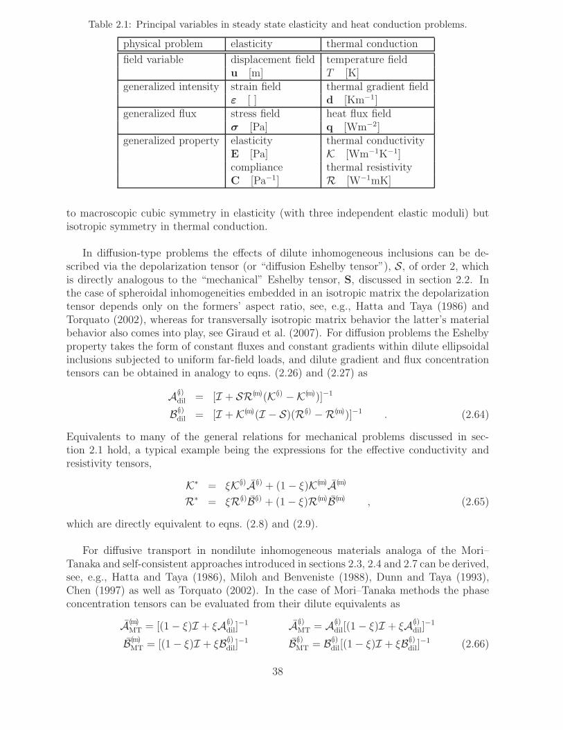
Table 2.1: Principal variables in steady state elasticity and heat conduction problems.

physical problem elasticity thermal conduction

field variable displacement field temperature fieldu [m] T [K]

generalized intensity strain field thermal gradient fieldε [ ] d [Km−1]

generalized flux stress field heat flux fieldσ [Pa] q [Wm−2]

generalized property elasticity thermal conductivityE [Pa] K [Wm−1K−1]compliance thermal resistivityC [Pa−1] R [W−1mK]

to macroscopic cubic symmetry in elasticity (with three independent elastic moduli) butisotropic symmetry in thermal conduction.

In diffusion-type problems the effects of dilute inhomogeneous inclusions can be de-scribed via the depolarization tensor (or “diffusion Eshelby tensor”), S, of order 2, whichis directly analogous to the “mechanical” Eshelby tensor, S, discussed in section 2.2. Inthe case of spheroidal inhomogeneities embedded in an isotropic matrix the depolarizationtensor depends only on the formers’ aspect ratio, see, e.g., Hatta and Taya (1986) andTorquato (2002), whereas for transversally isotropic matrix behavior the latter’s materialbehavior also comes into play, see Giraud et al. (2007). For diffusion problems the Eshelbyproperty takes the form of constant fluxes and constant gradients within dilute ellipsoidalinclusions subjected to uniform far-field loads, and dilute gradient and flux concentrationtensors can be obtained in analogy to eqns. (2.26) and (2.27) as

A(i)dil = [I + SR(m)(K(i) −K(m))]−1

B(i)dil = [I +K(m)(I − S)(R(i) −R(m))]−1 . (2.64)

Equivalents to many of the general relations for mechanical problems discussed in sec-tion 2.1 hold, a typical example being the expressions for the effective conductivity andresistivity tensors,

K∗ = ξK(i)A(i) + (1− ξ)K(m)A(m)

R∗ = ξR(i)B(i) + (1− ξ)R(m)B(m) , (2.65)

which are directly equivalent to eqns. (2.8) and (2.9).

For diffusive transport in nondilute inhomogeneous materials analoga of the Mori–Tanaka and self-consistent approaches introduced in sections 2.3, 2.4 and 2.7 can be derived,see, e.g., Hatta and Taya (1986), Miloh and Benveniste (1988), Dunn and Taya (1993),Chen (1997) as well as Torquato (2002). In the case of Mori–Tanaka methods the phaseconcentration tensors can be evaluated from their dilute equivalents as

A(m)MT = [(1− ξ)I + ξA

(i)dil]

−1 A(i)MT = A

(i)dil[(1− ξ)I + ξA

(i)dil]

−1

B(m)MT = [(1− ξ)I + ξB

(i)dil]

−1 B(i)MT = B

(i)dil[(1− ξ)I + ξB

(i)dil]

−1 (2.66)

38

in direct analogy to eqns. (2.29) and (2.30). Estimates for the effective conductivity tensoraccording to the classical self-consistent scheme takes the form

Kn+1 = K(m) + ξ[K(i) −K(m)][I + SnRn(K(i) −Kn)]−1

Rn+1 =[Kn+1

]−1, (2.67)

which is equivalent to eqn. (2.37). The differential scheme for the effective conductivitytensor can be written as

dK∗D

dξ=

1

1− ξ[K(i) −K∗

D]Adil(K∗D) , (2.68)

compare eqn. (2.39).

Replacement inhomogeneity models in analogy to section 2.8 can be used to handle theconduction behavior of composites containing non-ellipsoidal inhomogeneities as well asreinforcements with finite interfacial conductances. In the latter case, which is of consid-erable practical importance, provision must be made for the “replacement inhomogeneity”to account for the interfacial temperature jumps, see the discussion by Duschlbauer (2004).Replacement conductivities or resistivities must be evaluated from consistency conditionsequivalent to eqns. (2.62), i.e.,

K(i,r) = K(m) +1

ξdil

(K∗dil −K

(m))[A(i,r)dil ]−1

R(i,r) = R(m) +1

ξdil(R∗

dil −R(m))[B

(i,r)dil ]−1 . (2.69)

In contrast to standard methods for evaluating the effects of non-ideal interfaces on themacroscopic conductivity of composites (Hasselman and Johnson, 1987), the replacementinhomogeneity formalism can handle inhomogeneously distributed interfacial conductances(Nogales and Bohm, 2008). Both types of methods predict that finite interfacial conduc-tances give rise to a marked size effect in the macroscopic conductivities, i.e., below somecritical size even highly conductive reinforcements fail to improve the overall conductivityof composites. Diffusive transport in composites containing non-ellipsoidal inhomogeneitiescan also be described by resistance contribution tensors in analogy to the compliance con-tribution tensor formalism, eqn. (2.63).

Due to the lower rank of the tensors involved in diffusion-type problems the latter tendto be more benign and easier to handle than mechanical ones. Extensive discussions ofdiffusion-type problems in inhomogeneous media can be found, e.g., in Markov (2000),Torquato (2002) and Milton (2002). Analogous mean field descriptions can also be devisedfor a number of coupled problems, such as the electromechanical behavior of inhomoge-neous materials with at least one piezoelectric constituent, see, e.g., Huang and Yu (1994).

39

Chapter 3

Bounding Methods

Whereas mean field methods, unit cell approaches and embedding strategies can typicallybe used for both homogenization and localization tasks, bounding methods are limited tohomogenization. Discussions in this chapter again are restricted to materials consisting oftwo perfectly bonded constituents.

Rigorous bounds on the overall elastic properties of inhomogeneous materials are typ-ically obtained from appropriate variational (minimum energy) principles. In what fol-lows only outlines of bounding methods are given; formal treatments can be found, e.g.,in Nemat-Nasser and Hori (1993), Bornert (1996), Ponte Castaneda and Suquet (1998),Markov (2000), Torquato (2002) and Milton (2002).

3.1 Classical Bounds

Hill Bounds

Classical expressions for the minimum potential energy and the minimum complementaryenergy in combination with uniform stress and strain trial functions lead to the simplestvariational bounding expressions, the upper bounds of Voigt (1889) and the lower boundsof Reuss (1929). In their tensorial form (Hill, 1952) they are known as the Hill bounds andcan be written as [∑

(p)V (p)C(p)

]−1

≤ E ≤∑

(p)V (p)E(p) . (3.1)

These bounds, while universal and very simple, do not contain any information on themicrogeometry of an inhomogeneous material beyond the phase volume fractions, and aretoo slack for many practical purposes39. However, in contrast to the Hashin–Shtrikman andhigher-order bounds, they also hold for volume elements that are too small to be properRVEs.

39The bounds on the Young’s and shear moduli obtained from eqn. (3.1) are equivalent to Voigt andReuss expressions in terms of the corresponding phase moduli only if the constituents have Poisson’s ratiosthat give rise to equal Poisson contractions. Due to the homogeneous stress and strain assumptions used

for obtaining the Hill bounds, the corresponding phase strain and stress concentration tensors are A(p)V = I

and B(p)R = I, respectively.

40

Hashin–Shtrikman-Type Bounds

Considerably tighter bounds on the macroscopic behavior of inhomogeneous materials canbe obtained from a variational formulation due Hashin and Shtrikman (1961). They areformulated in terms of a homogeneous reference material and of polarization fields τ (x)that describe the difference between microscopic stress fields in the inhomogeneous materialand a homogeneous reference medium, compare eqn. (2.40). In combination with themacrohomogeneity condition, eqn. (1.6) polarization fields allow the complementary energyof the composite to be formulated in such a way that the “fast” and “slow” contributionsare separated, giving rise to the Hashin–Shtrikman variational principle. The latter canbe written in the form

FHS(τ (x)) =1

V

∫

V

τ T (x)[E0 − E(x)]−1 τ (x) + [τ (x)− 〈τ 〉∗]T ε′(τ (x)) + 2τ T ε0 dΩ ,

(3.2)compare, e.g., Gross and Seelig (2001). The definitions of the variables in eqn. (3.2) followthose in eqn. (2.40). The stationary values of FHS take the form

FHS = ε0T(E∗ −E0) ε0

and are maxima when (E(x) − E0) is positive definite and minima when (E(x) − E0) isnegative definite.

In order to allow an analytical solution for the above variational problem, the highlycomplex position dependent polarizations τ (x) are approximated by phase-wise constantpolarizations τ (p), compare eqn. (2.41). This has the consequence that the strain fluctua-tions ε′(τ (p)) can be evaluated by an Eshelby-type eigenstrain procedure. It can be shownthat for the case of isotropic constituents and isotropic overall behavior the proper Eshelbytensor to be used is the one for spheres. By optimizing the Hashin–Shtrikman variationalprinciple with respect to the τ (p) the tightest possible bounds within the Hashin–Shtrikmanscheme are found.

In the case of two-phase materials with isotropic constituents, in which the matrix issofter than the reinforcements, i.e., for (K(i) −K(m)) > 0 and (G(i) − G(m)) > 0, the aboveprocedure leads to lower bounds for the elasticity tensors of the form

E∗HS− = E(m) + ξ

[(E(i) −E(m))−1 + (1− ξ)S(m)C(m)

]−1

= E(m) + ξ(E(i) −E(m)) A(i)HS− , (3.3)

the strain concentration tensor A(i)HS− being equal to a Mori–Tanaka strain concentra-

tion tensor, eqn. (2.30), evaluated with a dilute concentration tensor of the type givenin eqn. (2.26). The upper bound Hashin–Shtrikman elasticity tensors are obtained byexchanging the roles of matrix and inhomogeneities as

E∗HS+ = E(i) + (1− ξ)

[(E(m) − E(i))−1 + ξS(i)C(i)

]−1

. (3.4)

41

The Hashin–Shtrikman bounds proper, eqn. (3.3) and (3.4), were stated by Hashinand Shtrikman (1963) in terms of bounds on the effective bulk modulus K∗ and the effec-tive shear modulus40 G∗. They apply to essentially all practically relevant inhomogeneousmaterials with isotropic phases that show (statistically) isotropic overall symmetry41 andfulfill the condition (K(i) −K(m))(G(i) − G(m)) > 0. The Hashin–Shtrikman formalism alsoallows to recover the Voigt and Reuss bounds when the reference material is chosen to bemuch stiffer or much softer than either of the constituents.

A different set of Hashin–Shtrikman bounds is applicable to (statistically) transverseisotropic composites reinforced by aligned continuous fibers42 (Hashin and Shtrikman,1962). For a discussion of evaluating these bounds for composites reinforced by trans-versely isotropic fibers see Hashin (1983).

Further developments led to the Walpole (1966) and Willis (1977) bounds, which per-tain to thermoelastically anisotropic overall behavior due to anisotropic constituents, sta-tistically anisotropic phase arrangements, and/or non-spherical reinforcements, a typicalexample being the aligned ellipsoidal microgeometry sketched in fig. 2.1. These boundsinclude the Hashin–Shtrikman bounds discussed above as special cases and they can alsohandle situations where a “softest” and “stiffest” constituent cannot be identified unequiv-ocally so that a fictive reference material must be used.

Hashin–Shtrikman-type bounds are not restricted to materials with matrix–inclusiontopologies, but hold for any phase arrangement of the appropriate symmetry and phasevolume fraction. In addition, it is worth noting that Hashin–Shtrikman-type bounds aresharp, i.e., they are the tightest bounds that can be given for the type of geometricalinformation used (volume fraction and overall symmetry, corresponding to two-point cor-relations). From the practical point of view it is of interest that for two-phase materialsMori–Tanaka estimates are equal to one of the Willis bounds (Weng, 1990), while the otherbound can be obtained after a “color inversion” (i.e., after exchanging the roles of inho-mogeneities and matrix)43. Accordingly, the bounds can be evaluated for fairly general

40Whereas engineers tend to describe elastic material behavior in terms of Young’s moduli and Poisson’sratios (which can be measured experimentally in a relatively straightforward way), many homogenizationexpressions are best formulated in terms of bulk and shear moduli, which directly describe the physicallyrelevant hydrostatic and deviatoric responses of materials. For obtaining bounds on the effective Young’smodulus E∗ from the results on K∗ and G∗ see Hashin (1983), and for bounding expressions on the Poissonnumbers ν∗ see Zimmerman (1992).

41Avellaneda and Milton (1989) constructed hierarchical laminates that are statistically isotropic butshow overall conductivities that do not fall within the pertinent Hashin–Shtrikman bounds. Accordingly,statistical isotropy by itself is not a sufficient condition for guaranteeing the validity of expressions suchas eqns. (3.3) and (3.4). For a discussion of Hashin–Shtrikman-type bounds of macroscopically isotropiccomposites consisting of anisotropic constituents see, e.g., Nadeau and Ferrari (2001).

42These bounds apply to general (transversely isotropic) two-phase materials, the (“in-plane”) phasegeometries of which are translation invariant in the “out-of-plane” or “axial” direction.

43Put more precisely, the lower bounds for two-phase materials are obtained from Mori–Tanaka methodswhen the more compliant material is used as matrix phase, and the upper bounds when it is used asinclusion phase. For matrix–inclusion materials with more than two constituents, Mori–Tanaka expressionsare bounds if the matrix is the stiffest or the softest phase, and fall between the appropriate boundsotherwise (Weng, 1990). Note, however, that extended Mori–Tanaka methods for nonaligned compositesas discussed in sections 2.7 and 2.8 in general do not coincide with bounds.

42

aligned phase geometries by simple matrix algebra such as eqn. (2.32). For elevated phasecontrasts the lower and upper Hashin–Shtrikman-type bounds tend to be rather far apart,however.

Composites reinforced by randomly oriented fibers or platelets follow the Hashin–Shtrikman bounds for statistically isotropic materials, eqns. (3.3) and (3.4). A discussionof Hashin–Shtrikman-type bounds on the elastic responses of composites with more generalfiber orientation distributions can be found in Eduljee and McCullough (1993). In the caseof porous materials (where the pores may be viewed as an ideally compliant phase) onlyupper Hashin–Shtrikman bounds can be obtained, the lower bounds for the elastic modulibeing zero. The opposite situation holds in case one of the constituents is rigid.

Hashin–Shtrikman-type variational formulations can also be employed for generatingbounds for more general phase arrangements. Evaluating the polarizations for “compositeregions” consisting of inhomogeneities embedded in matrix gives rise to Herve–Stolz–Zaouibounds (Herve et al., 1991). When complex phase patterns are to be considered (Bornert,1996; Bornert et al., 1996) numerical methods must be used for evaluating the polarizationfields.

Bounds for Discrete Microgeometries

Hashin–Shtrikman-type bounds can also be derived for (simple) periodic phase arrange-ments, see, e.g., Nemat-Nasser and Hori (1993). Among other bounding approaches forsuch phase arrangements are those of Bisegna and Luciano (1996), which uses approximatevariational principles evaluated from periodic unit cells via Finite Element models, and ofTeply and Dvorak (1988), which evaluates bounds for the elastoplastic behavior of fiberreinforced composites with periodic hexagonal phase arrangements.

3.2 Improved Bounds

When more complex trial functions are used in variational bounding, their optimizationrequires statistical information on the phase arrangement in the form of n-point corre-lations. This way improved bounds can be generated that are significantly tighter thanHashin–Shtrikman-type expressions.

Three-point bounds for statistically isotropic two-phase materials can be formulated insuch a way that the information on the phase arrangement statistics is contained in twothree-point microstructural parameters, η(ξ) and ζ(ξ), compare Torquato (2002). Evalu-ating these parameters for given arrangement statistics is a considerable task. However,analytical expressions or tabulated data in terms of the reinforcement volume fraction ξare available for a number of generic microgeometries of practical importance, among themstatistically homogeneous isotropic materials containing identical, bidisperse and polydis-perse impenetrable (“hard”) spheres (that describe matrix–inclusion composites) as wellas monodisperse interpenetrating spheres (“boolean models” that can describe many inter-woven phase arrangements), and statistically homogeneous transversely isotropic materials

43

reinforced by impenetrable or interpenetrating aligned cylinders. References to some three-point bounds and to a number of expressions for η and ζ applicable to some two-phasecomposites can be found in section 3.4, where results from mean field and bounding ap-proaches are compared. For reviews of higher-order bounds for elastic (as well as other)properties of inhomogeneous materials see, e.g., Quintanilla (1999), Torquato (1991) andTorquato (2002).

Improved bounds can provide highly useful information for low and moderate phasecontrasts (as typically found in technical composites), but even they tend to be ratherslack for elevated phase contrasts.

3.3 Bounds on Nonlinear Mechanical Behavior

Analoga to the Hill bounds for nonlinear inhomogeneous materials were introduced byBishop and Hill (1951). For polycrystals the nonlinear equivalents to Voigt and Reussexpressions are usually referred to as Taylor and Sachs bounds, respectively.

In analogy to mean field estimates for elastoplastic material behavior, nonlinear boundsare typically obtained by evaluating a sequence of linear bounds. Talbot and Willis (1985)extended the Hashin–Shtrikman variational principles to obtain one-sided bounds (i.e., up-per or lower bounds, depending on the material combination) on the nonlinear mechanicalbehavior of inhomogeneous materials.

An important development took place with the derivation of a variational principle byPonte Castaneda (1992) which provides upper bounds on the effective nonlinear behaviorof inhomogeneous materials on the basis of upper bounds for the elastic response44. Ituses a sequence of inhomogeneous reference materials, the properties of which have to beobtained by optimization procedures for each strain level. Essentially, the variational prin-ciple guarantees the best choice for the comparison material at a given load. The PonteCastaneda bounds are closely related to mean field approaches using improved secant plas-ticity methods, compare section 2.6. For higher-order bounds on the nonlinear response ofinhomogeneous materials see, e.g., Talbot and Willis (1998).

The study of bounds — like the development of improved estimates — for the overallnonlinear mechanical behavior of inhomogeneous materials has been an active field of re-search during the past decade, see the recent reviews by Suquet (1997), Ponte Castanedaand Suquet (1998) and Willis (2000).

44The Ponte Castaneda bounds are rigorous for nonlinear elastic inhomogeneous materials and, on thebasis of deformation theory, are very good approximations for materials with at least one elastoplastic con-stituent. Applying the Ponte Castaneda variational procedure to elastic lower bounds does not necessarilylead to a lower bound for the inelastic behavior.

44

3.4 Comparisons of Mean Field and Bounding

Predictions for Macroscopic Elastic Responses

In order to give some idea of the type of predictions that can be obtained by differentmean field (and related) approaches and by bounding methods for the thermomechanicalresponses of inhomogeneous thermoelastic materials, results for the overall elastic moduliand coefficients of thermal expansion are presented as functions of the reinforcement vol-ume fraction ξ in this section. All comparisons are based on E-glass particles or fibersembedded in an epoxy matrix. The elastic contrast of these constituents is c ≈ 21 and thethermal expansion contrast takes a value of approximately 0.14, see table 3.1.

Table 3.1: Constituent material parameters of epoxy matrix and E-glass reinforcements used ingenerating figs. 3.1 to 3.7.

E[GPa] ν[ ] α[1/K]matrix 3.5 0.35 36.0reinforcements 74.0 0.2 4.9

Figures 3.1 and 3.2 show predictions for the overall Young’s and shear moduli of aparticle reinforced composite using the above constituent parameters. The Hill boundscan be seen to be very slack. The Mori–Tanaka estimates (MTM) — as mentioned be-fore — coincide with the lower Hashin–Shtrikman bounds (H/S LB), whereas the classicalself-consistent scheme (CSCS) shows a typical behavior in that it is close to one Hashin–Shtrikman bound at low volume fractions, approaches the other at high volume fractions,and displays a transitional behavior in the form of a sigmoid curve in-between. The three-

0.0

40.0

EF

FE

CT

IVE

YO

UN

Gs

MO

DU

LUS

[GP

a]

0.0 0.2 0.4 0.6 0.8 1.0

PARTICLE VOLUME FRACTION []

Hill/Reuss LBHill/Voigt UBH/S LB; MTMH/S UB3PLB (mono/h)3PUB (mono/h)GSCS3PE (mono/h)CSCS

Figure 3.1: Bounds and estimates for the effective Young’s moduli of glass/epoxy particle rein-forced composites as functions of the particle volume fraction.

45

0.0

20.0

EF

FE

CT

IVE

SH

EA

R M

OD

ULU

S [G

Pa]

0.0 0.2 0.4 0.6 0.8 1.0

PARTICLE VOLUME FRACTION []

Hill/Reuss LBHill/Voigt UBH/S LB; MTMH/S UB3PLB (mono/h)3PUB (mono/h)GSCS3PE (mono/h)CSCS

Figure 3.2: Bounds and estimates for the effective shear moduli of glass/epoxy particle reinforcedcomposites as functions of the particle volume fraction.

point bounds (3PLB and 3PUB) shown in figs. 3.1 and 3.2 are based on formalisms de-veloped by Beran and Molyneux (1966), Milton (1981) as well as Phan-Thien and Milton(1983). They apply to impenetrable spherical particles of equal size and use expressionsfor the statistical parameters η and ζ that were reported by Miller and Torquato (1990)and Torquato et al. (1987), respectively. These expressions are available for reinforcementvolume fractions up to ξ = 0.645. The three-point estimates (3PE) of Torquato (1998)were evaluated with the same choice of η and ζ and can be seen to lie between the three-point bounds. For the case considered here the results from the generalized self-consistentscheme, which predicts a slightly stiffer behavior than the Mori–Tanaka method, are veryclose to the lower three-point bounds even though microgeometries corresponding to theGSCS are not monodisperse in the sizes of the inhomogeneities.

Predictions for the coefficients of thermal expansion of statistically isotropic inhomo-geneous materials are presented in fig. 3.3. Levin’s formula, eqn.(2.14), was combined theHashin–Shtrikman bounds, the three-point bounds and the three-point estimates for theeffective bulk modulus to obtain the corresponding bounds and estimates for the CTE.Because they are based on the same estimates for the effective bulk modulus, the resultsgiven for the GSCS and the Mori–Tanaka-scheme coincide with the upper Levin/Hashin–Shtrikman bounds.

In figs. 3.3 to 3.7 results are presented for the overall transverse Young’s moduli, overallaxial and transverse shear moduli, as well as overall axial and transverse coefficients of

45This value approaches the maximum volume fraction achievable in random packings of spheres, whichis ξ = 0.64 (Weisstein, 2000).

46

0.0

20.0

40.0

EF

FE

CT

IVE

CT

E [1

/K

]

0.0 0.2 0.4 0.6 0.8 1.0

PARTICLE VOLUME FRACTION []

H/S UB; MTMH/S LB3PUB (mono/h)3PLB (mono/h)GSCS3PE (mono/h)CSCS

−6x

10

Figure 3.3: Bounds and estimates for the effective CTEs of glass/epoxy particle reinforced com-posites as functions of the particle volume fraction.

0.0

40.0

EF

FE

CT

IVE

YO

UN

Gs

MO

DU

LUS

[GP

a]

0.0 0.2 0.4 0.6 0.8 1.0

FIBER VOLUME FRACTION []

Hill/Reuss LBHill/Voigt UBH/S LB; MTMH/S UB3PLB (mono/h)3PUB (mono/h)GSCS3PE (mono/h)CSCS

Figure 3.4: Bounds and estimates for the effective transverse Young’s moduli of glass/epoxy fiberreinforced composites as functions of the fiber volume fraction.

thermal expansion of composites reinforced by aligned continuous fibers46. The results forthe three-point bounds shown follow the formalism of Silnutzer (1972) and Milton (1981),

46In the case of the axial Young’s moduli the estimates and bounds are nearly indistinguishable from

each other (and from the rule of mixture result, E∗

A = ξE(i)A +(1− ξ)E(m), for the material parameters and

scaling used in fig. 3.4 and are, accordingly, not given here. It is, however, worth noting that the effectiveaxial Young’s modulus of a composite reinforced by aligned continuous fibers is always equal to or largerthan the rules of mixture result.

47

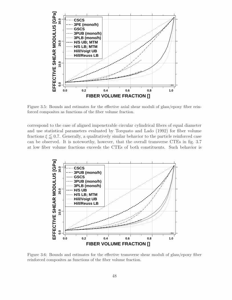
0.0

10.0

20.0

30.0

EF

FE

CT

IVE

SH

EA

R M

OD

ULU

S [G

Pa]

0.0 0.2 0.4 0.6 0.8 1.0

FIBER VOLUME FRACTION []

Hill/Reuss LBHill/Voigt UBH/S LB; MTMH/S UB; MTM3PLB (mono/h)3PUB (mono/h)GSCS3PE (mono/h)CSCS

Figure 3.5: Bounds and estimates for the effective axial shear moduli of glass/epoxy fiber rein-forced composites as functions of the fiber volume fraction.

correspond to the case of aligned impenetrable circular cylindrical fibers of equal diameterand use statistical parameters evaluated by Torquato and Lado (1992) for fiber volumefractions ξ / 0.7. Generally, a qualitatively similar behavior to the particle reinforced casecan be observed. It is noteworthy, however, that the overall transverse CTEs in fig. 3.7at low fiber volume fractions exceeds the CTEs of both constituents. Such behavior is

0.0

10.0

20.0

30.0

EF

FE

CT

IVE

SH

EA

R M

OD

ULU

S [G

Pa]

0.0 0.2 0.4 0.6 0.8 1.0

FIBER VOLUME FRACTION []

Hill/Reuss LBHill/Voigt UBH/S LB; MTMH/S UB3PLB (mono/h)3PUB (mono/h)GSCS3PUB (mono/h)CSCS

Figure 3.6: Bounds and estimates for the effective transverse shear moduli of glass/epoxy fiberreinforced composites as functions of the fiber volume fraction.

48

0.0

20.0

40.0

EF

FE

CT

IVE

CT

E [1

/K

]

0.0 0.2 0.4 0.6 0.8 1.0

FIBER VOLUME FRACTION [ ]

MTM ax.MTM tr.GSCS ax.GSCS tr.3PE (mono/h) ax.3PE (mono/h) tr.CSCS ax.CSCS tr.

−6x

10

Figure 3.7: Estimates for the effective axial and transverse CTEs of glass/epoxy fiber reinforcedcomposites as functions of the fiber volume fraction.

typical for continuously reinforced composites and is caused by the marked axial constraintenforced by the fibers.

In figs. 3.1 to 3.7 the classical self-consistent scheme — as expected — is not in goodagreement with the three-point bounds shown, which explicitly correspond to matrix–inclusion topologies. Considerably better agreement with the CSCS is found by usingthree-point parameters of the interpenetrating sphere or cylinder type (which can also de-scribe cases where both phases percolate, but are not as symmetrical with respect to theconstituents as the CSCS). From a practical point of view it is worth noting that despitetheir sophistication improved bounds (and higher order estimates) may give overly opti-mistic predictions for the overall moduli because they describe ideal composites, whereasin actual materials it is practically impossible to avoid flaws such as porosity.

Before closing this chapter it should be mentioned that more complex responses maybe obtained when one or both of the constituents are transversely isotropic with a highstiffness contrast between the axial and transverse directions (note that e.g. carbon fiberstypically exhibit transverse Young’s moduli that are much smaller than the Young’s moduliof, say, metallic matrices, whereas the opposite holds true for the axial Young’s moduli).Such effects may be especially marked in the nonlinear range. Also, the angular depen-dences of stiffnesses and CTEs in fiber reinforced materials can be quite rich, compare,e.g., Pettermann et al. (1997).

49

Chapter 4

General Remarks on ModelingApproaches Based on DiscreteMicrogeometries

In the following micromechanical approaches based on discrete microgeometries are un-derstood to encompass the periodic homogenization, embedding and windowing methodsdiscussed in chapters 5 to 7. Broadly speaking, these models trade off restrictions to thegenerality of the phase arrangements against the capability of using fine grained geomet-rical descriptions and of resolving details of the stress and strain fields at the length scaleof the inhomogeneities. The main fields of application of these methods are studying thenonlinear behavior of inhomogeneous materials and evaluating the microscopic stress andstrain fields of relevant microgeometries at high resolution. This information, on the onehand, may be required when the local stress and strain fields fluctuate strongly and are,accordingly, difficult to describe by averaged fields. On the other hand, it is importantfor understanding the damage and failure behavior of inhomogeneous materials, which candepend on details of their microgeometry.

4.1 Microgeometries

The heterogeneous volume elements (“microgeometries”) used in discrete microstructuremodels range from highly idealized periodic geometries, such as simple cubic arrays ofspheres in a matrix, to phase arrangements that aim at closely approximating the geo-metrical complexity of actual inhomogeneous materials. There are two philosophies forobtaining heterogeneous volume elements for modeling, viz., generating them by computeralgorithms or basing them directly on geometries obtained by experiment.

Computer Generated Phase Arrangements

Computer generated volume elements may be classified into two groups, one of which isbased on generic arrangements of a number of reinforcements that are randomly positionedand, where appropriate, randomly oriented. The other group aims at generating more spe-cific phase arrangements that have identical phase distribution statistics as some target

50

material. A further possible approach to generating realistic volume elements by computeralgorithms, which consists of modeling the actual production process, has seen little useto date for composites due to the complexity of the task.

The generation of generic microgeometrical models with random phase arrangementstypically involves random sequential addition methods46 and, in many cases, random per-turbation or relaxation techniques. The reinforcement volume fractions that can be reachedby RSA methods tend to be moderate due to jamming (geometrical frustration) and theirrepresentativeness for actual phase arrangements generated by mixing processes is opento question (Stroeven et al., 2004). Major improvements on both counts can be obtainedby using RSA geometries as starting configurations for random perturbation or hard coreshaking models (HCSM, also referred to as dynamic simulations), see, e.g., Buryachenkoet al. (2003), that apply small random displacements to each inhomogeneity to obtain moretightly packed arrangements of reinforcements as the size of the volume element is reducedto increase the inhomogeneity volume fraction. Methods of the above types have been usedto generate statistically homogeneous distributions of particular or fibrous reinforcements,see, e.g., Gusev (1997), Bohm and Han (2001), Lusti et al. (2002) or Duschlbauer et al.(2006), as well as idealized clustered microgeometries (Segurado et al., 2003).

The alternative strategy for generating volume elements by simulation aims at obtain-ing “statistically reconstructed” phase arrangements, which are not identical to any givensample, but rather are statistically equivalent to a target material. Statistical reconstruc-tion typically results in optimization problems in which some starting configuration (e.g., aperiodic phase arrangement of appropriate volume fraction) is modified such that suitablestatistical descriptors of the phase distributions closely approach or become equal to thechosen target descriptor. Procedures for reconstructing matrix–inclusion and more generalmicrogeometries have been reported that employ simulated annealing procedures (Rintouland Torquato, 1997; Torquato, 1998; Bochenek and Pyrz, 2002), genetic algorithms (Zemanand Sejnoha, 2001), and other minimization methods (Roberts and Garboczi, 1999). Forin-depth discussions of the underlying issues, such as statistical descriptors for the phasearrangements of inhomogeneous materials, see, e.g., Torquato (2002) and Zeman (2003).Statistical reconstruction studies have been based on a number of statistical descriptors ofphase arrangement, among them n-point distribution functions, radial distribution func-tions and correlation functions. Obviously, the statistical reconstruction of microgeometriesis closely connected to the concept of geometrical RVEs, compare section 1.3.

For volume elements that contain considerable numbers of inhomogeneities or other mi-crostructural features, statistically reconstructed phase arrangements are definitely morespecific to a given target material than are generic random microgeometries. However,because at present computational requirements put rather strong limits on the sizes of

46In random sequential addition (RSA) algorithms (also known as random sequential insertion or, in two-dimensional cases, random sequential adhesion models, and sometimes referred to as static simulations),positions and, where applicable, orientations for new reinforcements are created by random processes, acandidate inhomogeneity being accepted if it does not “collide” with any of the existing ones and rejectedotherwise. In contrast to random packing, in generating microgeometrical models a “collision” typicallyinvolves the violation of some minimum distance rather than an actual overlap between neighboring inho-mogeneities.

51

volume elements that can be handled by numerical engineering methods, this advantagetends to be limited in practice.

Computer generated microgeometries have tended to employ idealized reinforcementshapes, equiaxed particles embedded in a matrix, for example, being often represented byspheres, and fibers by cylinders or prolate spheroids47 of appropriate aspect ratio. Recentlywork employing polyhedral inhomogeneities has also been reported, see, e.g., (Nogales andBohm, 2008).

Real Structure Phase Arrangements

Instead of generating phase arrangements by computer algorithms, volume elements maybe chosen to follow as closely as possible the microgeometry in part of a given sampleof the material to be modeled, obtained from metallographic sections (Fischmeister andKarlsson, 1977), serial sections (Terada and Kikuchi, 1996; Li et al., 1999), tomographicdata (Hollister et al., 1994; Kenesei et al., 2004; Chawla and Chawla, 2006; Buffiere et al.,2008), etc. The resulting descriptions are often referred to as “real structure” models.

Recently the generation of real structure models from pixel (digital images) or voxel(tomographic) data describing the geometries of inhomogeneous materials has been the fo-cus of considerable research efforts. Such work typically has been based on digital images.It involves the steps of selecting from experimental data sets appropriate volume elementsfor analysis (“registration”) and of identifying the regions occupied by the different con-stituents by thresholding of the grey values of the pixels or voxels (“segmentation”). Atthis stage pixel or voxel models (compare section 4.2) can be generated directly from thesegmented data set or contouring procedures may be used for obtaining “smooth” phasedomains, the latter operation typically being more manpower intensive and difficult toautomatize. In the past decade tomography has proven especially useful for determiningthe microgeometries of inhomogeneous materials with constituents that show markedlydifferent X-ray absorption, e.g., porous and cellular materials.

Real microstructure models can provide accurate descriptions of actual phase arrange-ments, but they may depend to a considerable extent on details of the underlying experi-ments, e.g., the resolution of the digital images, and of the registration, segmentation and,where applicable, smoothing procedures. In general, they are non-periodic and, accord-ingly, cannot be used directly with the periodic homogenization techniques discussed insection 5.

47For uniform boundary conditions it can be shown that the overall elastic behavior of matrix–inclusiontype composites can be bounded by approximating the actual shape of particles by inner and outer en-velopes of “smooth” shape, e.g., inscribed and circumscribed ellipsoids. This is known as the Hill modi-fication theorem (or Hill’s comparison theorem, Hill’s auxiliary theorem), compare Hill (1963) and Huetet al. (1990). Approximations of actual inhomogeneity shapes by ellipsoids typically work considerablybetter for convex than for non-convex particle shapes (Kachanov and Sevostianov, 2005).

52

Sizes of Volume Elements

When complex discrete phase arrangements are employed in discrete microfield simula-tions the predicted macroscopic responses predicted from small volume elements has beenfound to show a marked dependence on colume element size, see, e.g., Iorga et al. (2008).This immediately raises the question of the size of volume element required for adequatelycapturing the macroscopic physical behavior of the material to be studied. On the onehand, the requirement of limiting numerical costs obviously puts a premium on using thesmallest viable volume element but, on the other hand, accuracy requirements are bestfulfilled by using close approximations to representative volume elements (RVEs, comparesection 1.3). These conflicting demands led to the concepts of “minimum RVEs” by Renand Zheng (2004) and of statistical RVEs (SRVEs) by Trias et al. (2006).

When the philosophy of geometrical RVEs is followed, the assessment of a suitablesize of volume element for analysis can be made on the basis of the microgeometry ofthe inhomogeneous material, the physical property to be modeled playing no role. In thiscontext adequate sizes of model geometries may be estimated, e.g., on the basis of exper-imentally obtained correlation lengths (Bulsara et al., 1999) or covariances (Jeulin, 2001)of the phase arrangement or by posing the requirement of having at least two statisticallyindependent inhomogeneities in the volume element (Zeman and Sejnoha, 2001). Suchapproaches have proven successful for micromechanical models of the elastic behavior ofinhomogeneous materials. The concept of physical RVEs, in contrast, implies that thesuitability of a given size of volume element for micromechanical modeling depends on thephysical property to be studied. This suitability can be assessed via windowing analysis,compare chapter 7, identical predictions of the macroscopic behavior with macroscopicallyhomogeneous stress and strain boundary conditions, respectively, being a necessary con-dition for physical RVEs. Weaker criteria involve comparisons of macroscopic properties(e.g., moduli) or responses (e.g., homogenized stress vs. strain curves) between differentvolume elements of equal size, or deviations from some macroscopic material symmetry.A comparison of different geometry and microfield based criteria for choosing the size ofmodel geometries was given by Trias et al. (2006).

Assessments based on geometry alone or on the overall elastic behavior predict thatrelatively small volume elements can give quite accurate results. Zeman (2003) reportedthat the transverse elastic behavior of composites reinforced by continuous fibers can besatisfactorily described by unit cells containing reconstructed arrangements of 10 to 20fibers. Using a nonlocal Hashin–Shtrikman model Drugan and Willis (1996) found thatfor statistically isotropic composites consisting of a matrix reinforced by spherical particlesvolume elements with sizes of some two and five particle diameters are sufficient for ob-taining errors of less than 5% and less than 1%, respectively, in terms of the macroscopicelastic behavior irrespective of the particle volume fraction. Considerably larger volumeelements are required for aligned ellipsoidal inhomogeneity, the independence of the modelsize from the volume fraction being lost (Monetto and Drugan, 2009).

When inelastic constituent behavior is present, however, a number of numerical studies(Zohdi, 1999; Jiang et al., 2001; Bohm and Han, 2001) have indicated that larger vol-ume elements may be required for satisfactorily approximating the overall symmetries and

53

obtaining good agreement, especially at elevated strains, between the responses of phasearrangements designed to be statistically equivalent. The reason for this behavior lies in themarked inhomogeneity of the microscopic strain fields that is typically present in nonlinearcomposites. For example, there tend to be contiguous zones of high plastic strains, whichcan evolve to become considerably larger than individual geometrical inhomogeneities, thuseffectively introducing a new length scale into the problem48.

When a number of volume elements of comparable size and pertaining to a given com-posite are available, they may be viewed as being realizations of some statistical process.In the typical case, where individual model geometries obtained by a computer model orfrom real structures are smaller than proper RVEs, ensemble averaging over a number ofresults obtained from such equivalent volume elements can be used to obtain improved esti-mates for the effective material properties, compare, e.g., Kanit et al. (2003) and Stroevenet al. (2004). The number of different volume elements required for a given accuracy ofthe ensemble averages decreases as the sizes of the models increase (Khisaeva and Ostoja-Starzewski, 2006). Finally, it is worth mentioning that the size of volume elements affectsnot only the macroscopic responses of composites but also the microfields, which tend tobe less sensitive to boundary condition effects when large phase arrangements are studied(Shen and Brinson, 2006).

4.2 Numerical Engineering Methods

The majority of published continuum micromechanical analyses of discrete microstructureshave employed standard numerical engineering methods for resolving the microfields. Workreported in the literature has used Finite Difference (FD) and Finite Volume algorithms,compare Adams and Doner (1967) and Bansal and Pindera (2006), spring lattice mod-els, compare Ostoja-Starzewski (1996), the Boundary Element Method (BEM), compareAchenbach and Zhu (1989) or Liu et al. (2005b), as well as the Finite Element Method(FEM) and its developments such as Extended Finite Element Methods, mesh-free andparticle methods, compare Sukumar et al. (2001) and Missoum-Benziane et al. (2007),or FE-based discrete dislocation models (Cleveringa et al., 1997). Generally speaking,spring lattice models tend to have advantages in handling pure traction boundary condi-tions and in modeling the progress of microcracks due to local (brittle) failure. Boundaryelements tend to be at their best in studying geometrically complex linear elastic problems.

In addition, techniques using Fast Fourier Transforms (FFT), compare Moulinec andSuquet (1994), and Discrete Fourier Transforms (DFT), compare Muller (1996), have beenused. They were mainly applied to analyzing periodic phase arrangements, for which theytend to be highly efficient, compare, e.g., Michel et al. (1999), and their fixed regular

48For elastoplastic matrices, weaker strain hardening tends to give rise to more inhomogeneous mi-crostrains, which leads to a requirement for bigger volume elements that contain a higher number ofinhomogeneities. Very large volumes tend to be necessary when one of the phases shows softening, e.g.,due to damage (Zohdi and Wriggers, 2001; Swaminathan and Ghosh, 2006; Gitman, 2006). Eliminatingthe dependence of the homogenized response on the size of the SRVE may, in fact, be impossible (Gitmanet al., 2007) in the latter case. For elastic polycrystals, the anisotropy and shape of the grains were alsoreported to influence the required size of volume elements (Ren and Zheng, 2004).

54

grids make them also well suited for for studying the evolution of microstructures (Dreyeret al., 1999). The Transformation Field Analysis of Dvorak (1992) allows the predictionof the nonlinear response of inhomogeneous materials based on either mean field descrip-tions (compare the remarks in section 2.6) or on discrete microfield approximations. Highcomputational efficiency is claimed for “classical” TFA models involving piecewise uni-form transformation fields (Dvorak et al., 1994), but very fine discretizations of the phasesare required to achieve good accuracy. A developed version of the TFA, the NonuniformTransformation Field Analysis (Michel and Suquet, 2004) expands anelastic strains intoa number of nonuniform, incompressible and orthogonal “plastic flow modes” to achieveefficient descriptions of the nonlinear mechanical behavior of inhomogeneous materials.

A number of further approaches that are specialized to continuum micromechanics arediscussed in connection with periodic microfield analyses, see section 5. For all numericalengineering methods the characteristic length of the discretization (“mesh size”) must beconsiderably smaller than the microscale of a given problem in order to obtain spatiallywell resolved results.

At present, the FEM is the most popular numerical scheme for evaluating discretemicrogeometries, especially in the nonlinear range, where its flexibility and capability ofsupporting a wide range of constitutive models for the constituents and for the interfacesbetween them are especially appreciated49. An additional asset of the FEM in the contextof continuum micromechanics is its ability to handle discontinuities in the stress and straincomponents (which typically occur at interfaces between different constituents) in a naturalway via appropriately placed element boundaries.

Applications of the FEM to micromechanical studies tend to fall into four main groups,compare fig. 4.1. In most published works the phase arrangements are discretized by an of-ten high number of “standard” continuum elements, the mesh being designed in such a waythat element boundaries (and, where appropriate, special interface elements) are positionedat all interfaces between constituents. Such approaches use unstructured meshes and havethe advantage that in principle any microgeometry can be discretized at a prescribed levelof accuracy. The resulting meshes are suitable for analysis with readily available commer-cial FE packages. However, the actual modeling of complex phase configurations in manycases requires sophisticated and/or specialized preprocessors for generating the mesh, atask that may be work intensive and has been found to be difficult to automatatize50. Inaddition, the resulting stiffness matrices may show unfavorable conditioning due to subop-timal element shapes and the requirement of satisfactory resolution of the microfields atlocal “hot spots” (e.g., between closely neighboring reinforcements) can lead to very largemodels indeed. Nevertheless, the possibility of providing for mesh refinements where they

49Constitutive models for constituents used in FEM-based micromechanics have included a wide range ofelastoplastic, viscoelastoplastic and continuum damage mechanics descriptions as well as crystal plasticitymodels, see, e.g., McHugh et al. (1993), and nonlocal models, compare Bassani et al. (2001) and Drabekand Bohm (2006). In addition, the FEM has supported a range of modeling options for interfaces betweenphases.

50Most preprocessors for Finite Element analysis are not geared towards discretizing matrix–inclusiontopologies with thin matrix bridges between closely approaching inclusions. Other major sources of difficul-ties are intersections between phase and cell boundaries at very acute or obtuse angles and the generationof periodic meshes for PMAs.

55

a) b) d)c)

Figure 4.1: Sketch of FEM approaches used in micromechanics: a) discretization by standardelements, b) special hybrid elements, c) pixel/voxel discretization, d) “multi-phase elements”

are required and of using standard mesh refinement approaches are major strengths of thisdiscretization strategy.

Alternatively, a smaller number of special hybrid elements may be used, which arespecifically formulated to model the deformation, stress, and strain fields in an inhomoge-neous region consisting of a single inhomogeneity or void together with the surroundingmatrix on the basis of some appropriate analytical theory (Accorsi, 1988). The mosthighly developed approach of this type at present is the Voronoi Finite Element Method(Ghosh et al., 1996), in which the mesh for the hybrid elements is obtained from Voronoitessellations based on the positions of the reinforcements. Large planar multi-inclusionarrangements can be analyzed this way using a limited number of (albeit rather complex)elements, and good accuracy as well as significant gains in efficiency have been claimed.Numerous damage models have been implemented into the method and an extension tothree dimensions was reported recently (Ghosh and Moorthy, 2004). Modeling approachesof this type are specifically tailored to inhomogeneous materials with matrix–inclusiontopologies.

A computational strategy that occupies an intermediate position between the abovetwo approaches uses static condensation to remove the degrees of freedom of the interiornodes of the inhomogeneities (or, in the case of coated reinforcements, of inhomogeneitiesand interface) from the stiffness matrix of a heterogeneous volume element (Liu et al.,2005a).

Especially when the phase arrangements to be studied are based on digital images ofactual microgeometries, a third approach for discretizing microgeometries of interest. Itconsists of using a structured mesh that consists of regular, rectangular or hexahedral el-ements of fixed size and has the same resolution as the digital data, each element being

56

assigned to one of the constituents by operations such as thresholding of the grey valuesof the corresponding pixel or voxel, respectively. Such meshes have the advantage of al-lowing a straightforward automatic model generation from appropriate experimental data(metallographic sections, tomographic scans) and of avoiding ambiguities in smoothing thedigital data (which are generally present if a “standard” FE mesh is employed to discretizeexperimental data of this type). Obviously “pixel element” and “voxel element” strategieslead to ragged phase boundaries, which may give rise to some oscillatory behavior of thesolutions (Niebur et al., 1999), can cause high local stress maxima (Terada et al., 1997),may degrade accuracy, and restrict detailed modeling of interfacial effects. Such “digitalimage based” (DIB) models are, however, claimed not to cause unacceptably large errorseven for relatively coarse discretizations, at least in the linear elastic range (Guldberget al., 1998). Good spatial resolution, i.e., a high number of pixels or voxels, of course, isespecially beneficial in such models.

A fourth approach also uses structured FE meshes, but assigns phase properties at theintegration point level of standard elements (“multi-phase elements”), see, e.g., Schmauderet al. (1996) or Quilici and Cailletaud (1999). Essentially, this amounts to trading offragged boundaries at element edges for smeared-out (and typically degraded) microfieldswithin those elements that contain a phase boundary, because stress or strain disconti-nuities within elements cannot be adequately handled by standard FE shape functions.With respect to the element stiffnesses the latter concern can be much reduced by over-integrating elements containing phase boundaries, which leads to good approximationsof integrals involving non-smooth displacements by numerical quadrature, see Zohdi andWriggers (2001). The resulting stress and strain distributions, however, remain smeared-out approximations in elements that contain phase boundaries, the rate of convergence ofthe microfields being accordingly slow. Multiphase element models also are limited in theircapabilities for detailed modeling of interfaces. Some of the above drawbacks are avoidedby algorithmic developments such as Extended Finite Element methods, which use a back-ground mesh that does not have to conform to phase boundaries, which are accounted for,e.g., by appropriately enriching the shape functions (Moes et al., 2003).

A fairly recent development for studying microgeometries involving a considerable num-ber of inhomogeneities (tens to thousands) by Finite Element methods involves programsspecially geared towards solving micromechanical problems. Such codes may be based onmatrix-free iterative solvers such as Conjugate Gradient (CG) methods, analytical solu-tions for the microfields (e.g., constant strain approximations corresponding to the upperHill bounds, eqn. (3.1), being used as starting solutions to speed convergence51. For stud-ies involving such programs see, e.g., Gusev (1997), Zohdi and Wriggers (2001) or Arbenzet al. (2008). Fast solvers of this type open the possibility of solving inverse problems, e.g.,for finding optimal particle shapes for given load cases and damage modes, compare Zohdi(2003).

Special Finite Element formulations (and, as a consequence, dedicated Finite Elementprograms) are typically required for asymptotic homogenization models (compare section5.3) and for other schemes that concurrently solve the macroscopic and microscopic prob-

51Essentially, in such a scheme the initial guess gives a good estimate of “long wavelength” contributionsto the solution, and the CG iterations take care of “short wavelength” variations.

57

lems, see, e.g., Urbanski (1999).

Discrete microgeometry approaches employing numerical engineering methods are bestsuited for phase arrangements in which the characteristic lengths of important geometricalfeatures do not differ markedly. If this is not the case, very large volume elements maybe required, meshing tends to become very difficult, and the numerical effort for studyingthe models may become excessive, especially for three-dimensional configurations. Typicalcases in point are composites reinforced by short fibers with aspect ratios in excess of, say,25 or by polydispersely sized particles for which the minimum and maximum diametersdiffer by more than a factor of, say, 5.

4.3 Evaluation of Results

When elastic or thermoelastic inhomogeneous materials are studied, the major aim ofhomogenization in discrete microstructure approaches consists in evaluating the effectivetensors, E∗ and α∗. In homogenization studies of elastoplastic, thermoelastoplastic orviscoelastoplastic materials, in contrast, usually the evolution of appropriate scalar macro-scopic variables is followed, e.g., in the form of stress–strain diagrams52.

In general six linearly independent mechanical load cases must be applied to the vol-ume element for evaluating macroscopic elastic tensors, and a homogeneous temperaturechange is required for obtaining the macroscopic thermal expansion tensor. The effectiveelastic tensors of inhomogeneous materials with orthotropic or higher symmetry show thesame structure as those of isotropic or transversely isotropic symmetry, see eqns. 1.9 and1.10, i.e., in Nye notation all terms are zero with the exception of the upper left submatrixand the diagonal of the lower right submatrix. However, volume elements corresponding toreal structures or obtained with stochastics-based computer models in general show lowersymmetries. This is mainly due to their limited size, which introduces “sub-orthotropic”contributions into the elastic matrix that are smaller than the “orthotropic contributions”discussed above, but do not vanish. In addition, small perturbations of the tensor elementsdue to roundoff errors in the numerical engineering methods must be expected.

Accordingly, volume elements aimed at describing statistically isotropic, transverselyisotropic or orthotropic material behavior actually return lower material symmetries. Theseerrors, which tend to decrease with growing size of the volume elements, can in principle becorrected by looking for that elastic tensor of the required symmetry which is closest to the“raw” elastic tensor evaluated from homogenization, resulting in optimization problems.Little pertinent work, however, has been published. Pahr and Bohm (2008) proposed asimplified approach in which the sub-orthotropic contributions to the elastic tensor of aunit cell like the one shown in fig. 5.4, which aims at describing a statistically isotropiccomposite, is coarsely “orthotropized” by setting all sub-orthotropic terms to zero and,

52Homogenized tangent tensors for given load states can also be evaluated, compare, e.g., (Ghosh et al.,1996). This is of interest mainly in multi-scale analysis employing discrete microstructure models asimplicit material models for Finite Element models on the macroscale.

58

if necessary, symmetrizing the “raw tensor”53. The closest isotropic tensor to such an“orthotropized” elastic tensor can then be obtained as the isotropic term of a generalizedspherical harmonics expansion of the orthotropic elongation and bulk modulus orientationdistribution functions, using expressions developed by He and Curnier (1997); for an al-ternative approach to finding the isotropic tensor that is closest to an elasticity tensor ofgeneral anisotropy see Norris (2006). Moduli evaluated from the resulting “isotropized”elasticity tensor provide better approximations to effective moduli than do averages over,say, tensile responses in the coordinate directions.

Microscopic fields can usually be directly obtained from the numerical engineering meth-ods. Some care is necessary, however, because, on the one hand, the extreme values ofmicroscopic stresses and strains tend to depend markedly on details of the microgeometryand, on the other hand, idiosyncrasies of the numerical methods may come into play. Forexample, due to limitations in the extrapolation and averaging algorithms used by FiniteElement methods stresses and strains tend to be evaluated with lower accuracy at phaseboundaries than within bulk phases.

For evaluating phase averaged quantities from unit cell analyses, it is good practice touse direct volume integration according to eqn. (1.13)54. In many FE codes this can bedone by approximate numerical quadrature according to

〈f〉 =1

Ω

∫

Ω

f(z)dΩ ≈1

Ω

N∑

l=1

fl Ωl (4.1)

Here fl and Ωl are the function value and the integration weight (in terms of the volumeof the integration point), respectively, associated with the l-th integration point within agiven integration volume Ω that contains N integration points55 When macroscopic valuesor phase averages are to be generated of variables that are nonlinear functions of thestress or strain components (e.g., equivalent stresses, equivalent strains, stress triaxialities),only direct volume averaging should be used, because evaluation of nonlinear variables onthe basis of averaged components may lead to unacceptable inaccuracies, compare alsosection 2.6. Besides generating overall and phase averages, microscopic variables can alsobe evaluated in terms of averages in individual inhomogeneities. In addition, distributionfunctions (“stress spectra”, see, e.g., Bornert et al. (1994), Bohm and Rammerstorfer (1995)or Bohm and Han (2001)) and higher statistical moments of microfields can be evaluatedfrom discrete microstructure models for the whole composite, for a given phase or forindividual inhomogeneities, compare the fiber level standard deviations of the maximumprincipal stress displayed in fig. 2.3.

53Actually, in finding the orthotropic elasticity tensor that is closest to a “raw” elastic tensor the ori-entations of the former’s principal axes must also be considered. In “raw” elastic tensors obtained byperiodic homogenization, compare section 5, typically only very small deviations from symmetry due toroundoff errors are found, whereas applying windowing methods, compare section 7, to sub-orthotropicvolume elements can give rise to considerably higher anisotropies.

54It is of some practical interest that volume averaged and phase averaged microfields obtained fromdiscrete microfield analysis must fulfill all relations given in section 2.1 and can thus be conveniently usedto check the consistency of a given model by inserting them into eqns. (2.5). Note, however, that for finitedeformations appropriate stress and strain measures must be used for this purpose (Nemat-Nasser, 1999).

55Such procedures may also be used for evaluating other volume integrals, e.g., in computing Weibull-type fracture probabilities for reinforcements (Antretter, 1998; Bohm et al., 2002).

59

Chapter 5

Periodic Microfield Models

Periodic Microfield Approaches (PMAs) aim at approximating the macroscopic and micro-scopic behavior of inhomogeneous materials by studying model materials that have periodicmicrostructures.

5.1 Basic Concepts of Unit Cell Models

Periodic microfield approaches analyze the behavior of infinite (one, two- or three-dimensio-nal) periodic phase arrangements under the action of far field mechanical loads or uniformtemperature fields56. The most common approach for studying the stress and strain fieldsin such periodic configurations is based on describing the microgeometry by a periodicallyrepeating unit cell57 (RUC) to which the investigations may be limited without loss ofinformation or generality, at least for static analysis58.

The literature on periodic microfield models of inhomogeneous materials is fairly ex-tensive, and well developed mathematical theories are available on scale transitions inperiodic structures, compare Michel et al. (2001). A wide variety of unit cells have been

56Standard PMAs cannot handle macroscopic gradients in mechanical loads, temperature or compositionin any direction in which periodicity of the fields is prescribed. Gradients and free boundaries can bestudied, however, in directions where periodicity is not prescribed, a typical case being layer-type modelsthat are non-periodic in one direction and periodic in the other(s), see, e.g., Wittig and Allen (1994),Reiter et al. (1997) and Weissenbek et al. (1997).

57In the present work the designation “unit cell” is used for any volume element that can generate aperiodic microgeometry. Accordingly, a unit cell may comprise a simple periodic base unit (or part ofit), a collective of simple periodic base units, or a phase arrangement of arbitrary geometrical complexity(multi-fiber or multi-particle unit cell) that shows translational periodicity. With increasing size unit cellsapproximate geometrical and/or physical RVEs increasingly more closely.

58Periodic phase arrangements are typically not well suited to dynamic analysis, because they act asfilters that exclude all waves with frequencies outside certain bands, see, e.g., Suzuki and Yu (1998). Inaddition, due to the boundary conditions required for obtaining periodicity, unit cell methods can onlyhandle wavelengths that are smaller than or equal to the relevant cell dimension, and only standing wavescan be dealt with.In analogy, in stability analysis unit cells can directly resolve only buckling modes of specific wavelengths,so that considerable care is required in using them for such purposes, compare Vonach (2001) as well asPahr and Rammerstorfer (2006). However, bifurcation modes with wavelengths exceeding the size of theunit cell can be resolved in periodic linear models by using the Bloch theorem from solid state physics(Gong et al., 2005).

60

employed in such studies, ranging from geometries that describe simple periodic arrays ofinhomogeneities to highly complex phase arrangements, such as multi-inhomogeneity unitcells (“supercells”). For some simple periodic phase arrangements and for linear materialbehavior it has proved possible to find analytical solutions based on series expansions thatmake explicit use of the periodicity (Sangani and Lu, 1987; Cohen, 2004) or on appropriatepotential methods (Wang et al., 2000).

Even though most PMA studies in the literature have used standard numerical engi-neering methods as described in chapter 4, other numerical schemes have been proposedthat are specialized to periodic phase arrangements. One of them, known as the Method ofCells (Aboudi, 1989, 1991), in its basic form discretizes unit cells that correspond to squarearrangements of square fibers into four subcells, within each of which displacements areapproximated by low-order polynomials. Traction and displacement continuity conditionsat the faces of the subcells are imposed in an average sense and analytical and/or semi-analytical approximations to the deformation fields are obtained in the elastic and inelasticranges. While using highly idealized microgeometries, providing only limited informationon the microscopic stress and strain fields, and having limited capabilities for handlingaxial shear, the resulting models pose relatively low computational requirements and canbe used as a constitutive model for analyzing structures made of continuously reinforcedcomposites, see, e.g., Arenburg and Reddy (1991). Developments of the algorithm led tothe Generalized Method of Cells (Aboudi, 1996), which is more flexible geometrically andallows finer discretizations of unit cells for fiber and particle reinforced composites, rein-forcement and matrix being essentially split into a number of “subregions” of rectangularor hexahedral shape. For some comparisons with microfields obtained by Finite Elementbased unit cells see, e.g., Iyer et al. (2000) or Pahr and Arnold (2002). Recently, higherorder displacement interpolants were introduced to obtain the High-Fidelity GeneralizedMethod of Cells (Aboudi, 2004), which provides an alternative to Finite Element algo-rithms for “pixel element” micromechanical models (compare section 4.2).

A further group of solution strategies for PMAs reported in the literature (Axelsen andPyrz, 1995; Fond et al., 2001; Schjødt-Thomsen and Pyrz, 2004) use numerically evaluatedequivalent inclusion approaches that account for interacting inhomogeneities as provided,e.g., by the work of Moschovidis and Mura (1975). Alternatively, the elastic fields in peri-odic inhomogeneous materials can be evaluated numerically via variational approaches fordetermining stress-free strain fields (Wang et al., 2002).

In periodic homogenization the strain and stress fields are decomposed into constantmacroscopic strain and stress contributions (“slow variables”), 〈ε〉 and 〈σ〉, and period-ically varying microscopic fluctuations (“fast variables”), ε′(z) and σ′(z), in analogy toeqn. (1.1). Here z is a “microscopic coordinate” that has sufficient resolution for describ-ing the variations on the microscale. The corresponding expression for the displacementstakes the form (Michel et al., 1999)

u(z) = 〈ε〉z + u′(z) . (5.1)

Volume integrals for obtaining averages, eqns.(1.3) and (1.5), must, of course, be solvedover the volume of the unit cell, ΩUC. Formal derivations of the above relationships for

61

periodically varying microstrains and microstresses show that the work done by the fluc-tuating stress and strain contributions vanishes, compare Michel et al. (2001).

Evidently, in periodic microfield approaches each unit of periodicity (unit cell) con-tributes the same increment of the displacement vector ∆u so that the homogenized dis-placements vary (multi)linearly. An idealized depiction of such a situation is presented infig. 5.1, which shows the variations of the strains εs(s) = 〈εs〉+ε

′s(s) and of the correspond-

ing displacements us(s) = 〈εs〉 s + u′s(s) along some line s in a hypothetical periodic two-phase material consisting of constituents A and B. Obviously, the relation 〈εs〉 = ∆us/cuholds for linear displacement–strain relations, where cu stands for the length of a unit cellin direction s and ∆us for the corresponding displacement increment. The periodicity ofthe strains and of the displacements is immediately apparent.

s

uε,

<ε >su’

<ε >’ε

∆us

A A AB B B A

s

ss

s

cu

Figure 5.1: Schematic depiction of the variation of the strains εs(s) and the displacements us(s)along a generic “one-dimensional composite” (coordinate s) consisting of constituents A and B.Symmetry points of εs(s) and us(s) are indicated by small circles.

5.2 Boundary Conditions

Unit cells together with the boundary conditions (B.C.s) prescribed on them must generatevalid tilings both for the undeformed geometry and for all deformed states pertinent tothe investigation. Accordingly, gaps and overlaps between neighboring unit cells as wellas unphysical constraints on their deformations must not be allowed, i.e., the cells mustbe geometrically compatible. In order to achieve this, the boundary conditions for theunit cells must be specified in such a way that all deformation modes appropriate for theload cases to be studied can be attained. The three major types of boundary conditionsused in periodic microfield analysis are periodicity, symmetry, and antisymmetry (or point

62

symmetry) B.C.s59. In PMA models one of these three types of boundary conditions (ora combination of them) must be used, irrespective of the numerical method employed forsolving the equilibrium equations.

Generally, for a given periodic phase arrangement unit cells are non-unique, the rangeof possible shapes being especially wide when point or mirror symmetries are present inthe microgeometry. As an example, fig. 5.2 depicts a (two-dimensional) periodic hexagonalarray of circular inhomogeneities (e.g., fibers oriented normally to the plane) and someof the unit cells that can be used to study aspects of the behavior of this phase arrange-ment. There are considerable differences in the sizes and capabilities of the unit cells shown.

2

1 periodic boundarysymmetry boundarypoint symmetry boundary

symmetry center(pivot point)

AB

F

GC

H I

D

E

J

Figure 5.2: Periodic hexagonal array of circular inhomogeneities in a matrix and 10 unit cellsthat can be used to describe the mechanical responses of this arrangement under loads actingparallel to the coordinate axes.

In the following a nomenclature is used in which the faces of two-dimensional quadri-lateral unit cells are denoted as N, S, E and W (for North, South, East, and West whichare used as in topographical maps), vertices being named according to the adjoining cellfaces, compare figs. 5.5, 5.6 and 5.7. The faces of three-dimensional cells of hexahedralshape are, in analogy, referred to as N, S, E, W, B and T (the latter standing for bottomand top), and edges as well as vertices are referred to by the adjoining faces (e.g., SE orSWB), see fig. 5.4.

59For more formal treatments of boundary conditions for unit cells than given here see, e.g., Anthoine(1995) or Michel et al. (1999). In the case of layer-type models, which can be generated by specifying freesurfaces at appropriate boundaries, macroscopic rotational degrees of freedom, i.e., macroscopic bendingand twisting, can be studied by appropriately modifying the above standard B.C.s. When such macroscopicrotational degrees of freedom are present, out-of-plane shear loads must be accompanied by appropriatebending moments to achieve stress equilibrium, compare, e.g., Urbanski (1999).

63

Periodicity Boundary Conditions

The most general boundary conditions for unit cells in continuum micromechanics are pe-riodicity (“toroidal”, “cyclic”) B.C.s, which can handle any physically valid deformationstate of the cell and, consequently, of the inhomogeneous material to be modeled. Peri-odicity boundary conditions make use of translatoric symmetries of a given geometry; infig. 5.2 cells A to E belong to this group.

In order to describe an N -dimensional phase arrangement with translatoric periodicity,a suitable unit cell and a set of N linearly independent periodicity vectors pn are required.These periodicity vectors are neither unique nor do they have to be orthogonal. For anygiven periodic microgeometry the minimum volume of pertinent unit cells is well defined,but such “minimum unit cells” can take a wide range of shapes as is shown for a simpletwo-dimensional case in fig. 5.3. The surface of each proper unit cell must consist of at leastN pairs of faces (or parts of faces) Γk, and the surface elements making up a pair, k− andk+, must be identical but shifted relative to each other by “shift vectors” ck. Each shiftvector, in turn, must be a linear combination of the periodicity vectors, i.e., ck =

∑l c

kl pl,

where the ckl are integer numbers. In fig. 5.3 pairs of faces (or, in the case of some cell,parts of faces) Γk are marked by being drawn with the same line style.

p

p + p

p1

2

1 2

Figure 5.3: Six different but equivalent periodic minimum-size unit cells for a two-dimensionalperiodic matrix–inclusion medium with two (slightly) non-orthogonal translation vectors p1 andp2. Paired faces (or parts of faces) Γk are marked by identical line styles and regions belongingto one of the cells are highlighted by shading.

Computer generated periodic volume elements are often set up such that the trans-lation vectors are orthogonal, which allows to generate unit cells that are rectangles orright hexahedra, compare fig. 5.4. Unit cells of simple shape to some extent facilitate theapplication of periodicity boundary conditions. However, low-angle intersections betweenphase boundaries and cell faces as well as phase boundaries that closely approach cell facesoften make such cells difficult to mesh for FE analysis. This issues can be alleviated oravoided by choosing suitably shaped and positioned unit cells.

64

NEB

SEB

NWT

NET

SWB

SWT

Figure 5.4: Cube-shaped periodic unit cell containing 15 randomly positioned spherical particlesof equal size at a volume fraction of ξ(i)=0.15. Designators of the six faces (East, West, North,South, Top, Bottom) and of the vertices are given (Pahr and Bohm, 2008).

Because the unit cells tile the computational space by translation, neighboring cells(and, consequently, the “opposite” faces of a given cell) must fit into each other like thepieces of a jigsaw puzzle in both undeformed and deformed states. For each pair of sur-face elements, Γk, eqn.(5.1) allows to express the boundary conditions for the mechanicalproblem in the small strain regime as

∆uk = uk+ − uk− = u(sk + ck)− u(sk) = 〈ε〉 ∗ ck , (5.2)

where uk+ and uk− are the displacements at corresponding points sk + ck and sk of thesurface elements k+ and k− (which could, e.g., correspond to that faces N and S in fig. 5.4),respectively. sk is a local coordinate on surface element k− and 〈ε〉 is the macroscopicstrain, which is prescribed in displacement controlled analysis and must be determined inload controlled analysis. These conditions enforce a “seamless fit” between neighboringunit cells for all possible deformed states.

For the special case of initially rectangular two-dimensional unit cells, such as the oneshown in fig. 5.5, this leads to the expressions

uN(s1) = uS(s1) + uNW uE(s2) = uW(s2) + uSE , (5.3)

where vertex SW is assumed to be fixed. Equations (5.3) directly imply that

uNE = uNW + uSE .

For numerical analysis the two faces making up a pair Γk must be discretized in a com-patible way, i.e., the nodal points on then must be positioned at equal values of the “facecoordinates” sk. Equations (5.2) then become sets of linear constraints each of which links

65

three nodal displacement DOFs60. Comparing eqns.(5.2) and (5.3) shows that the dis-placements of the “master nodes” SE and NW contain the information on the macroscopicstrain tensor 〈ε〉. In addition, the displacements of the master nodes and of faces S andW fully control the displacements of the “slave faces” N and E.

Conditions analogous to eqn. (5.3) can be specified for any periodic, space-filling andregular two-dimensional cell that has an even number of sides (squares, rectangles, andhexagons) or three-dimensional cell that has an even number of faces (cubes, hexahedra,rhombic dodecahedra, and regular tetrakaidecahedra). The scheme can also be extended tounit cells of less regular shape that have even numbers of faces, compare Cruz and Patera(1995) or Xia et al. (2003) as well as figs. 5.2 and 5.3. Periodicity B.C.s generally are theleast restrictive option for multi-inhomogeneity unit cell models using phase arrangementsgenerated by statistics-based algorithms.

In practice FE-based unit cell studies using periodicity boundary conditions can berather expensive in terms of computing time and memory requirements, because the multi-point constraints required for implementing eqn. (5.3) or its equivalents tend to degradethe band structure of the system matrix, especially in three-dimensional problems. Inaddition it is worth noting that — especially for simple phase arrangements — care maybe required to prevent over- and underconstraining due to inappropriate selection of regionswith periodicity boundary conditions, compare Pettermann and Suresh (2000).

Symmetry Boundary Conditions

For rectangular and hexahedral unit cells in which the faces of the cell coincide withsymmetry planes of the phase arrangement and for which this property is retained for alldeformed states that are to be studied, periodicity B.C.s simplify to symmetry boundary

60In principle, all variables (i.e., for mechanical analysis the displacements, strains and stresses) must belinked by appropriate periodicity conditions. When a displacement based FE code is used, however, suchconditions can be specified explicitly only for the displacement components (including, where appropriate,rotational DOFs). The periodicity of the stresses is then typically fulfilled only approximately, mainlybecause in most implementations nodal stresses are not averaged across cell boundaries, even though theyought to be.As a consequence of the periodicity of stresses the traction vectors at unit cell boundaries are antiperiodic.

NW

SE

NE

SW

NEu

SEu

N

W E

S

uNW

s

s1

2

~

~

Figure 5.5: Sketch of periodicity boundary conditions as used with an initially rectangular two-dimensional unit cell.

66

conditions. Following the nomenclature of fig. 5.6 these B.C.s take the form

uE(s2) = uSE vN(s1) = vNW uW(s2) = 0 vS(s1) = 0 , (5.4)

where u and v stand for the displacement components in 1- and 2-direction, respectively.Equation (5.4) puts constraints on the normal components of the at the unit cells’ surfaces,but leaves the tangential displacements free, thus enforcing the condition that pairs of mas-ter and slave faces must stay parallel throughout the deformation history. For symmetryB.C.s there are no requirements with respect to compatibility of phase arrangements ormeshes at different faces.

NW

SW

NE

SE

NEu

SEu

~s

s~EW

N

S

uNW

1

2

Figure 5.6: Sketch of symmetry boundary conditions as used with a rectangular two-dimensionalunit cell.

Symmetry boundary conditions are fairly easy to use and tend to give rise to small unitcells for simply periodic phase arrangements. However, the load cases that can be handledare limited to uniform thermal loads, mechanical loads that act in directions normal toone or more pairs of faces, and combinations of the above61. In fig. 5.2 unit cell F usesboundary conditions of this type. Symmetry boundary conditions are typically very usefulfor describing relatively simple microgeometries, but tend to be restrictive for modelingphase arrangements generated by statistics-based algorithms or obtained from micrographs.

Antisymmetry Boundary Conditions

Antisymmetry (or point symmetry) boundary conditions require the presence of centersof point symmetry (“pivot points”) and are, accordingly, even more limited in terms ofthe microgeometries that they can handle. In contrast to symmetry boundary conditions,however, unit cells employing them on all faces are subject to few restrictions with respectto the load cases that can be handled. Among the unit cells shown in fig. 5.2, cells Gand H use point symmetry B.C.s on all faces and can handle any in-plane deformation62.

61Because these load cases include different normal loads acting on each pair of faces, loading by macro-scopic extensional shear (obtained, e.g., in the two-dimensional case by applying normal stresses σa to thevertical and −σa to the horizontal faces), hydrostatic loading, and (hygro)thermal loading, symmetry B.C.sare typically sufficient for materials characterization. However, for macroscopically anisotropic materialsthe normal and shear stresses evaluated as above do not pertain to the same coordinate system becauseextensional shear corresponds to simple shear in a coordinate system rotated by 45.

62Triangular unit cells similar to cell H in fig. 5.2 were used, e.g., by Teply and Dvorak (1988) to studythe transverse mechanical behavior of hexagonal arrays of fibers. Rectangular cells with point symmetries

67

Alternatively, antisymmetry B.C.s can be combined with symmetry B.C.s to obtain verysmall unit cells that are restricted to loads acting normal to the symmetry faces, compareunit cells I and J in fig. 5.2. Figure 5.7 shows such a “reduced” unit cell, the antisymmetryboundary conditions being applied on face E where a pivot point P is present. For thisconfiguration the boundary conditions

uU(sP) + uL(−sP) = 2uP

vN(s1) = vNW = 2vP vS(s1) = 0 uW(s2) = 0 , (5.5)

must be fulfilled, where uU(sP) and uL(−sP) are the displacement vectors of pairs of pointsU and L that are positioned symmetrically with respect to the pivot point P. As indicatedin fig. 5.7 the local coordinate system s is defined on face E and centered on P. Theundeformed geometry of such a face also must be antisymmetric with respect to the pivotpoint P, and the phase arrangements as well as the discretizations on both halves of faceE must be compatible. Three-dimensional unit cells employing combinations of symmetryand point symmetry B.C.s can, e.g., be used to advantage for studying cubic arrays ofparticles, see Weissenbek et al. (1994).

SW

NWUu

Lu

~s

Pus~

W

S

NuNW

~s

SE

NE

E

L

U

P

1

2

p

Figure 5.7: Sketch of a quadrilateral two-dimensional unit cell that combines antisymmetryboundary conditions on face E with symmetry boundary conditions on faces N, S and W.

Within the nomenclature of fig. 5.7, the displacements at the master nodes SE and NW,uSE and uNW, control the overall deformation of the unit cell in the 1- and 2-directionsand can be used to evaluate the macroscopic strain of the corresponding periodic modelmaterial, compare eqn. (5.15). With respect to unit cell models that use the FEM forevaluating the microfields, it is worth noting that all of the above types of boundary con-ditions can be handled by any code that provides linear multipoint constraints betweendegrees of freedom and thus allows the linking of three or more D.O.F.s by linear equations.

Obviously, the description of real materials, which in general are not periodic, by peri-odic model materials entails some geometrical approximations. In the case of real structuregeometries this may entail applying periodicity constraints to non-periodic geometries ormodifying the geometries such that they become periodic63. The effects of such approxi-mations are perturbations in the vicinity of the cell surfaces which diminish in importance

on each boundary were introduced by Marketz and Fischer (1994) for perturbed square arrangements ofinhomogeneities. The periodic cells D and E also show point symmetry on their faces.

63The simplest way of “periodifying” a non-periodic rectangular or cuboidal volume element consists

68

with growing size of the model. At least in the linear range the use of windowing withappropriate mixed boundary conditions, compare chapter 7, provides a superior alternativeto such ad-hoc “periodification” procedures.

Periodicity boundary conditions that are conceptually similar to eqn. (5.3) can bedevised for cases where standard conditions for homogenization are not met, gradient(nonlocal) theories are employed on the macroscale, and higher-order stresses as well asstrain gradients figure in coupling the length scales (Geers et al., 2001b).

5.3 Application of Loads and Evaluation of Fields

Once suitable unit cells have been defined and appropriate boundary conditions applied,the volume elements must be subjected to appropriate loads in the form of macroscopicstresses, strains and/or temperature excursions, i.e., the microscopic and macroscopic fieldsmust be linked. Whereas loading by uniform temperature differences does not pose majordifficulties, applying far field stresses or strains is not necessarily straightforward. Forexample, the variations of the stresses along the faces of a unit cell in general are not knowna priori, so that it is not possible to prescribe the boundary tractions via distributed loads.There are two major approaches to implementing the micro–macro linkage.

Asymptotic Homogenization

The most versatile and elegant strategy for linking the macroscopic and microscopic fields inperiodic microfield models is based on a mathematical framework referred to as asymptotichomogenization, asymptotic expansion homogenization, or homogenization theory, see,e.g., Suquet (1987). It is based on explicitly introducing macroscopic and microscopiccoordinates, Z and z, respectively, into the formulation of the problem. The microscopicand macroscopic coordinates are linked by the expression

zi = xi/ǫ (5.6)

where ǫ = ℓ/L ≪ 1 is a scaling parameter. L and ℓ stand for the characteristic lengthsof the macro- and microscales64. The displacement field in the unit cell can then berepresented by an asymptotic expansion of the type

ui(Z, z, ǫ) = u(0)i (Z) + ǫ u

(1)i (Z, z) + ǫ2 u

(2)i (Z, z) + H.O.T. , (5.7)

where the u(0)i are the effective or macroscopic displacements and u

(1)i stands for the peri-

odically varying displacement perturbations due to the microstructure65.

in mirroring it with respect to 2 or 3 of its surfaces, respectively, and doing periodic homogenization onthe resulting larger unit cell. Such operations, however, tend to lead to undesired shapes of reinforcementand to changes in the arrangement statistics. The alternative expedient of specifying symmetry B.C.s forrectangular or cuboidal real structure cells amounts to an even larger modification of the microgeometryand introduces marked local constraints. Nevertheless, for sufficiently large multi-inhomogeneity cellsuseful results can be obtained with the latter strategy, see, e.g., (Terada et al., 2000).

64Equation (5.6) may be viewed as “stretching” the microscale so it becomes comparable to themacroscale, f(x)→ f(Z,Z/ǫ) = f(Z, z).

65The nomenclature used in eqns. (5.6) to (5.13) follows typical usage in asymptotic homogenization.It is more general than but can be directly compared with the one used in eqns. (1.1) to (5.5), where nomacroscopic coordinates Z are employed.

69

Using the chain rule, i.e.,

∂

∂xf(Z(x), z(x), ǫ) →

∂

∂Zf +

1

ǫ

∂

∂zf , (5.8)

the strains can be related to the displacements in the small strain elastic regime as

εij(Z, z, ǫ) =1

2

(∂

∂Zj

u(0)i +

∂

∂Zi

u(0)j

)+

(∂

∂zj

u(1)i +

∂

∂zi

u(1)j

)

+ǫ

2

(∂

∂Zj

u(1)i +

∂

∂Zi

u(1)j

)+

(∂

∂zj

u(2)i +

∂

∂zi

u(2)j

)+ H.O.T.

= ε(1)ij (Z, z) + ǫ ε

(2)ij (Z, z) + H.O.T. , (5.9)

where terms of the type ε(0)ij = 1

ǫ∂

∂zju

(0)i are deleted due to the underlying assumption that

the variations of slow variables are negligible at the microscale. In analogy the stresses canbe expanded into the expression

σij(Z, z, ǫ) = σ(1)ij (Z, z) + ǫ σ

(2)ij (Z, z) + H.O.T. . (5.10)

Using the two-scale assumption and, as a consequence, eqn. (5.8), the equilibrium equationstake the form ( ∂

∂Zj

+1

ǫ

∂

∂zj

)σij(Z, z, ǫ) + fi(Z) = 0 , (5.11)

the fi being macroscopic body forces. By inserting eqn. (5.10) into this expression and sort-ing the resulting terms by order of ǫ a hierarchical system of partial differential equationsis obtained

∂

∂zj

σ(1)ij = 0 (order ǫ−1)

∂

∂Zj

σ(1)ij +

∂

∂zj

σ(2)ij + fi = 0 (order ǫ0) , (5.12)

the first of which gives rise to a boundary value problem at the unit cell level that is referredto as the “micro equation”. By making a specific ansatz for the strains at unit cell leveland by volume averaging over the second equation in the system (5.12), which is known asthe “macro equation”, the microscopic and macroscopic fields can be linked such that thehomogenized elasticity tensor is obtained as

Eijkl =1

ΩUC

∫

ΩUC

Eijkl(z)[Iklmn +

∂

∂zl

χkmn(z)]dΩ . (5.13)

Here ΩUC is the volume of the unit cell, Eijkl(z) is the phase-level (microscopic) elasticitytensor, and the “characteristic function” χkmn(z) describes the deformation modes of theunit cell66 and, accordingly, relates the micro- and macrofields. Analogous expressions canbe derived for the tangent modulus tensors used in elastoplastic analysis, compare Ghosh

66Even though eqns. (5.12) and (5.13) are derived from an explicit two-scale formulation neither of themcontains the scale parameter ǫ, see the discussion by Chung et al. (2001).

70

et al. (1996).

The above relations can be used as the basis of Finite Element algorithms that solve forthe characteristic function χijk(z), a task that typically has required special analysis codes.For detailed discussions of asymptotic homogenization methods within the framework ofFEM-based micromechanics see, e.g., Hollister et al. (1991), Ghosh et al. (1996), Hassaniand Hinton (1999) or Chung et al. (2001). An asymptotic homogenization procedure forelastic composites that uses standard elements within a commercial FE package was pro-posed by Banks-Sills and Leiderman (1997).

Asymptotic homogenization allows to directly couple FE models on the macro- andmicroscales, compare, e.g., Ghosh et al. (1996) or Terada et al. (2003), an approach thathas been used in a number of multi-scale studies (compare chapter 8) and is sometimesreferred to as the FE2 method (Feyel, 2003). A treatment of homogenization in the vicinityof macroscopic boundaries can be found in Schrefler et al. (1997). Asymptotic homoge-nization schemes have also been employed for problems involving higher-order stresses andstrain gradients (Kouznetsova et al., 2002)67, an approach referred to as higher order ho-mogenization.

Recently, an alternative unit-cell based asymptotic homogenization scheme for linearproblems, the Variational Asymptotical Method for Unit Cell Homogenization (VAMUC),was reported (Yu and Tang, 2007), which can also be implemented within a Finite Elementframework.

Method of Macroscopic Degrees of Freedom

When asymptotic homogenization is not used, it is good practice to apply far field stressesand strains to a given unit cell via concentrated nodal forces or prescribed displacements,respectively, at the master nodes and/or pivot points, an approach termed the “method ofmacroscopic degrees of freedom” by Michel et al. (1999). Employing the divergence theoremand using the nomenclature and configuration of fig. 5.5, for load controlled analysis theforces to be applied to the master nodes SE and NW, PSE and PNW, of a two-dimensionalunit cell with periodicity boundary conditions can be shown to be given by the surfaceintegrals

PSE =

∫

ΓE

ta(z) dΓ PNW =

∫

ΓN

ta(z) dΓ . (5.14)

67Such methods are especially useful for problems in which the length scales are not well separated; inthem the “unit cells” do not necessarily remain periodic during the deformation process.

71

Here ta(z) = σa ∗nΓ(z) stands for the homogeneous surface traction vector correspond-ing to the applied (far field) stress field68 at some given point z on the cell’s surface ΓUC, andnΓ(z) is the local normal vector of the appropriate face. Equation (5.14) can be generalizedto require that each master node is loaded by a force corresponding to the surface integralof the surface traction vectors over the face slaved to it via an equivalent of eqns. (5.14),compare Smit et al. (1998). Analogous procedures hold for three-dimensional cases, andsymmetry as well as antisymmetry boundary conditions as described by eqns. (5.4) and(5.5) can be handled by eqn. (5.14).

For applying far field strains to periodic volume elements, the displacements to be pre-scribed to the master nodes must be obtained from the macroscopic strains via appropriatestrain–displacement relations. For example, using the notation of eqns. (5.3), the displace-ments to be prescribed to the master nodes NE and SW of the unit cell shown in fig. 5.5can be evaluated from eqn. (5.2) as

uSE = εa11 c1 vSE = γa

12 c1

uNW = γa21 c2 vNW = εa

22 c2 (5.15)

for an applied strain εa and linear strain–displacement relations69. For the case consideredhere, the projections of the shift vectors, c1 and c2, are equal to the side lengths of the cellin the undeformed state. In order to obtain the elastic tensors of periodic phase arrange-ments, six linearly independent load cases must be evaluated. Typically strain controlledunit cell analysis is easier to handle than stress controlled models70.

In general, the overall stress and strain tensors within a unit cell can be evaluated byvolume averaging71 or by using the equivalent surface integrals given in eqn. (1.3), i.e.,

〈σ〉 =1

ΩUC

∫

ΩUC

σ(z) dΩ =1

ΩUC

∫

ΓUC

t⊗ z dΓ

〈ε〉 =1

ΩUC

∫

ΩUC

ε(z) dΩ =1

2ΩUC

∫

ΓUC

(u⊗ nΓ + nΓ ⊗ u) dΓ . (5.16)

In practice, it is typically fairly straightforward to evaluate volume integrals by numericalintegration schemes such as eqn. (4.1), whereas no comparable approximations are avail-able for surface integrals.

68Note that the ta(z) are not identical with the actual local values of the tractions, t(z), at the cellboundaries, but are equal to them in an integral sense over the cell face. For geometrically nonlinearanalysis eqn. (5.14) must be applied to the current configuration. Because the far field stress σa isconstant it can be factored out of the surface integrals, so that the force applied to a master node PM

takes the form PM = σa ∗∫ΓS

nΓ(z) dΓ, which is the projection of the applied stress to the current averagesurface normal of the slave face ΓS times the current area of the face.

69Equations (5.15) can be directly extended to three-dimensional problems and to handling nonlinearstrain–displacement relations as well as deformation gradients (Huber et al., 2007).

70Even though the loads acting on the master nodes obtained from eqn. (5.14) are equilibrated, in stresscontrolled analysis solid body rotations may be induced through small numerical errors. When these solidbody rotations are suppressed by deactivating degrees of freedom beyond those required for enforcingperiodicity, the quality of the solutions may be degraded or transformations of the averaged stresses andstrains may be required.

71For large strain analysis the consistent procedure is to first average the deformation gradients andthen evaluate the strains from these averages.

72

In the case of rectangular or hexahedral unit cells that are aligned with the coordinateaxes, averaged engineering stress and strain components can, of course, be evaluated bydividing the applied or reaction forces at the master nodes by the appropriate surface ar-eas and by dividing the displacements of the master nodes by the appropriate cell lengths,respectively.

5.4 Unit Cell Models for Composites Reinforced by

Continuous Fibers

Unit cell modes have been reported for three groups of continuously reinforced composites,unidirectionally reinforced, angle-ply and cross-ply materials as well as fabric reinforcedcomposites.

Composites Reinforced by Unidirectional Continuous Fibers

Composites reinforced by continuous aligned fibers typically show a statistically trans-versely isotropic overall behavior and can be studied well with periodic homogenization.Materials characterization with the exception of the overall axial shear behavior can be car-ried out with two-dimensional unit cell models employing generalized plane strain elementsthat use a global degree of freedom to describe the axial deformation of the whole model72.For handling the overall axial shear response special generalized plane strain elements(Adams and Crane, 1984; Sørensen, 1992) or three-dimensional analyses with appropriateboundary conditions (Pettermann and Suresh, 2000) are required73. Three-dimensionalmodeling is also relevant for the materials characterization of composites reinforced bycontinuous aligned fibers when the effects of fiber misalignment, of fiber waviness (Garnichand Karami, 2004), or of broken fibers74 (Mahishi, 1986) are to be studied. Unit cell modelsused for nonlinear constitutive modeling, of course, must be fully three-dimensional andemploy periodicity boundary conditions.

Basic generalized plane strain models of continuously reinforced composites make useof simple periodic fiber arrangements as shown in fig. 5.8, all of which can be described byrather small unit cells using symmetry and/or antisymmetry B.Cs. The simplest amongthese arrangements are the periodic hexagonal (PH0) and periodic square (PS0) arrays.Models with hexagonal symmetry (PH0,CH1,RH2,CH3) give rise to transversely isotropicthermoelastic overall behavior, whereas the other fiber arrangements shown in fig. 5.8

72Generalized plane strain elements suitable for such analysis are implemented in a number of commercialFE codes. Because the axial stiffness of composites reinforced by continuous aligned fibers can usually besatisfactorily described by Voigt-type (“rule of mixture”) models unit cell studies of such materials havetended to concentrate on the transverse behavior. Note that plain strain models can describe neither theaxial constraints nor the axial components of microstresses and microstrains.

73For linear elastic material behavior there is the additional option of making use of the formal analogybetween out-of-plane (antiplane) shear and diffusion problems.

74For investigating the axial failure behavior of continuously reinforced MMCs, statistical methodsconcentrating on fiber fragmentation or more elaborate spring lattice models, see, e.g., Zhou and Curtin(1995), have been used successfully.

73

PH0CH1RH2CH3

PS0MS5CS7CS8

Figure 5.8: Eight simple periodic fiber arrangements of fiber volume fraction ξ=0.475 for modelingcontinuously fiber reinforced composites (Bohm and Rammerstorfer, 1995).

have tetragonal (PS0,CS7,CS8) or monoclinic (MS5) overall symmetry. In the elastoplas-tic range the macroscopic symmetries of the fiber arrangements degrade under most loadcases, see fig. 5.9. This behavior is due to the low symmetry of the local material propertiesof the matrix (especially the plastic strain and, as a consequence, the strain hardening),which depend on the load history a given point has undergone. In many cases simpleperiodic microgeometries do not provide satisfactory descriptions of fiber reinforced mate-rials, most of which show at least some randomness in the fiber positions. Much improvedmodels can be obtained by periodic multi-fiber unit cells that employ quasi-random fiberpositions. Such models can either use symmetry B.C.s, compare the unit cell shown infig. 5.10, which is based on the work of Nakamura and Suresh (1993), or periodicity B.C.s(Moulinec and Suquet, 1997; Gusev et al., 2000; Zeman and Sejnoha, 2007).

In table 5.1 thermoelastic moduli of an aligned continuously reinforced ALTEX/AlMMC as predicted by bounding methods, MFAs and unit cells methods using arrangementsPH0, CH1 and PS0 (compare fig. 5.8) as well as DN (see fig. 5.10) are listed. For thismaterial combination all unit cell results (even PS0, which is not transversally isotropic)fall within the Hashin–Shtrikman bounds75, but the predictions for the square arrangementshow clear in-plane anisotropy and do not follow the three-point bounds. The resultsfor the multi-fiber arrangement indicate some minor deviation from transversely isotropicmacroscopic behavior.

The fiber arrangements shown in figs. 5.8 and 5.10 give nearly identical results for theoverall thermoelastoplastic behavior of continuously reinforced composites under axial me-chanical loading, and the predicted overall axial and transverse responses under thermal

75The constituents’ material properties underlying table 3 show a low elastic contrast of C ≈ 3, makingthem relatively insensitive to perturbations of macroscopic symmetry. In general the elastic stiffnessesobtained from square-type arrangements may violate the Hashin–Shtrikman bounds and usually lie outsidethe three-point bounds.

74

0.0

0E+0

0 1

.00E

+01

2.0

0E+0

1 3

.00E

+01

4.0

0E+0

1 5

.00E

+01

6.0

0E+0

1

AP

PLI

ED

ST

RE

SS

[MP

a]

0.00E+00 5.00E-04 1.00E-03 1.50E-03 2.00E-03 2.50E-03 3.00E-03 3.50E-03 4.00E-03

STRAIN []

ALTEX FIBERAl99.9 MATRIXPH0/00PH0/90PS0/00PS0/45DN/00

Fiber

Matrix

PS/45

PH

DNPS/00

Figure 5.9: Transverse elastoplastic response of a unidirectional continuously reinforced AL-TEX/Al MMC (ξ=0.453, elastoplastic matrix with linear hardening) to transverse uniaxial load-ing as predicted by unit cell models PH0, PS0 and DN.

loading are also very similar. The overall behavior under transverse mechanical loading,however, depends markedly on the phase arrangement, see fig. 5.9. For fiber arrangementsof tetragonal or lower symmetry (e.g., PS0, MS5, CS7 and CS8) the predicted transversestiffness depends strongly on the loading direction. The behavior of the hexagonal arrange-ments is sandwiched between the stiff (0) and the compliant (45) responses of periodicsquare arrangements in both the elastic and elastoplastic ranges. Multi-fiber unit cellsthat approach statistical transverse isotropy (such as the one shown in fig. 5.10) tend toshow noticeably stronger strain hardening compared to periodic hexagonal arrangements,

EPS.EFF.PLASTIC INC.800

2.25E-02

1.75E-02

1.25E-02

7.50E-03

2.50E-03

Figure 5.10: Microscopic distributions of the accumulated equivalent plastic strain in the matrixof a transversely loaded unidirectional continuously reinforced ALTEX/Al MMC (ξ=0.453) aspredicted by a multi-fiber unit cell (arrangement DN).

75

Table 5.1: Overall thermoelastic moduli of a unidirectional continuously reinforced ALTEX/AlMMC (ξ=0.453 nominal) as predicted by the Hashin–Shtrikman (HS) and three-point (3PB)bounds, by the Mori–Tanaka method (MTM) and the generalized self-consistent scheme (GSCS),by Torquato’s three-point estimates (3PE), as well as by unit cell analysis using periodic arrange-ments shown in fig. 5.8 (PH0, CH1, PS0) and the multi-fiber cell displayed in fig. 5.10 (DN). Forarrangement PS0 responses in the 0 and 45, and for arrangement DN responses in the 0 and90 directions are listed.

E∗A E∗

T ν∗A ν∗T α∗A α∗

T

[GPa] [GPa] [] [] [K−1×10−6] [K−1×10−6]fibers 180.0 180.0 0.20 0.20 6.0 6.0matrix 67.2 67.2 0.35 0.35 23.0 23.0HS/lo 118.8 103.1 0.276 0.277 — —HS/hi 119.3 107.1 0.279 0.394 — —3PB/lo 118.8 103.8 0.278 0.326 — —3PB/hi 118.9 104.5 0.279 0.347 — —MTM 118.8 103.1 0.279 0.342 11.84 16.46GSCS 118.8 103.9 0.279 0.337 11.84 16.463PE 118.8 103.9 0.279 0.338 11.89 16.40PH0 118.8 103.7 0.279 0.340 11.84 16.46CH1 118.7 103.9 0.279 0.338 11.90 16.42PS0/00 118.8 107.6 0.279 0.314 11.85 16.45PS0/45 118.8 99.9 0.279 0.363 11.85 16.45DN/00 118.8 104.8 0.278 0.334 11.90 16.31DN/90 118.8 104.6 0.278 0.333 11.90 16.46

of the same fiber volume fraction, compare Moulinec and Suquet (1997). Generally themacroscopic yield surfaces of uniaxially reinforced MMCs are not of the Hill (1948) type,but can be described by a bimodal description (Dvorak and Bahei-el Din, 1987).

The distributions of microstresses and microstrains in fibers and matrix tend to dependstrongly on the fiber arrangement, especially under thermal and transverse mechanicalloading. In the plastic regime, the microscopic distributions of equivalent and hydrostaticstresses, equivalent plastic strains and stress triaxialities tend to be markedly inhomoge-neous76, see, e.g., fig. 5.10. As a consequence of the inhomogeneity of the microfields, theretend to be strong constrained plasticity effects in continuously reinforced MMCs and theonset of damage in the matrix, of fracture of the fibers, and of interfacial decohesion atthe fiber–matrix interfaces show a strong dependence on the fiber arrangement.

Cross-Ply and Angle-Ply Composites

Another group of composite materials reinforced by continuous fibers that can be studiedto advantage by unit cell methods are laminates consisting of plies the thickness of whichis not much greater than the fiber diameter. The left side of fig. 5.11 depicts a unit cell

76The corresponding distribution functions, phase averages, and higher statistical moments are alsosignificantly influenced by the fiber arrangement, compare Bohm and Rammerstorfer (1995).

76

for a cross-ply laminate with double layers of fibers which is suitable for use with period-icity and symmetry boundary conditions. In the the center a minimum unit cell for cross

o90 plies

β

o0 ply

Figure 5.11: Unit cell for a double layer cross-ply laminate (left), minimum unit cell for a crossply-laminate (center) and unit cell for an angle-ply laminate with ply angle β (right).

ply laminates with one fiber layer per ply is shown, which requires the use of symmetryboundary conditions. A unit cell for studying angle-ply laminates with a general ply angleβ via periodicity boundary conditions is displayed on the right side of fig. 5.11.

Unit cells with symmetry boundary conditions were used for studying the thermome-chanical behavior of cross ply laminates by Lerch et al. (1991) as well as Ismar and Schroter(2000). For unit cell studies of angle ply laminates see Xia et al. (2003) and Abolfathi et al.(2008).

Fabric Reinforced Composites

Periodic microfield methods have played an important role in modeling the behavior offabric reinforced composites, i.e., materials containing woven, braided, or knitted rein-forcements. In such “textile composites” the reinforcing phase usually takes the form oftextile-like structures consisting of bundles of continuous fibers (tows). Unit cell modelsfor such materials are typically based on modeling fiber bundles as a “mesophase” withsmeared out material properties, which, in turn, are obtained from analyzing unidirection-ally continuously reinforced composites77. Free surface boundary conditions are typicallyspecified for the out-of-plane faces of the cell, and a number of cells may be stacked ontop of each other in order to account for in-plane offsets and constraint effects betweenthe layers (Bystrom et al., 2000). Symmetry boundary conditions can be specified for thein-plane faces, which gives reasonably small unit cells as shown in fig. 5.12, but restrictsthe load cases that can be handled in in-plane normal and thermal loads. By applyingextended periodicity boundary conditions to larger unit cells macroscopic rotational de-grees of freedom can be introduced to allow studying all deformation models, including themacroscopic warping and twisting of the laminae.

There is a wide range of weaves as well as knitting and braiding architectures that canbe modeled with PMAs. Unit cells for woven, knitted and braided composites tend to befairly complex geometrically, may be difficult to mesh for Finite Element analysis and may

77This modeling strategy obviously is a type of multiscale modeling as discussed in chapter 8.

77

TowsCompositeMatrix

Figure 5.12: A unit cell for modeling a plain weave lamina using symmetry boundary conditions.The tow region (left), the matrix region (center) and the “assembled” unit cell (right) are shown.

pose considerable computational requirements, especially when nonlinear behavior is tobe studied. Over the past 20 years a considerable number of studies have been publishedon unit cell modeling of fabric reinforced composites, see, e.g., Cox and Flanagan (1997),Huang and Ramakrishna (2000), Tang and Whitcomb (2003) or Lomov et al. (2006), andon software for generating appropriate unit cells (Robitaille et al., 2003; Sherburn, 2007).

5.5 Unit Cell Models for Short Fiber Reinforced Com-

posites

The overall symmetry of short fiber reinforced composites in many cases is isotropic (forrandom fiber orientations) or transversely isotropic (for aligned fibers, planar random fibersand other fiber arrangements with axisymmetric orientation distributions). However, pro-cessing conditions can give rise to a wide range of fiber orientation distributions and,consequently, lower overall symmetries (Allen and Lee, 1990). The thermoelastic and ther-moelastoplastic behavior of aligned short fiber reinforced composites has been successfullyestimated by Mori–Tanaka methods, which can also be extended to nonaligned fibers andreinforcements showing an aspect ratio distribution, compare section 2.7. Such mean-fieldapproaches are, however, limited in resolving details of fiber arrangements, especially forinelastic material behavior. At present the most powerful tools for studying the influenceof fiber shapes and orientations, of clustering effects, of the interaction of fibers of dif-ferent sizes, and of local stress and strain fields between neighboring fibers are periodicmicrofield methods. Platelet reinforced composites can be described in analogy to shortfiber reinforced materials.

Composites Reinforced by Aligned Short Fibers

In contrast to continuously reinforced composites, the phase arrangements of discontinu-ously reinforced materials are inherently three-dimensional. The simplest three-dimensionalunit cell models of aligned short fiber reinforced composites have used periodic square ar-

78

rangements of non-staggered or staggered aligned cylindrical fibers78, see, e.g., Levy andPapazian (1991) and compare fig. 5.13. Such geometries are relatively simple to set up anddo not pose major computational requirements, but are rather restrictive in terms of fiberarrangements and load conditions that can be handled. By setting up larger unit cells sup-porting periodicity boundary conditions are used the full thermomechanical behavior of thefiber arrangements can be studied. Analogous microgeometries based on periodic hexago-nal arrangements of non-staggered (Jarvstrat, 1992) or staggered (Tucker and Liang, 1999)fibers as well as ellipsoidal unit cells aimed at describing composite “ellipsoid assembly”microgeometries (Jarvstrat, 1993) were also proposed79.

Figure 5.13: Three-dimensional unit cells for modeling non-staggered (left) and staggered (right)square arrangements of aligned short fibers. The shaded cells require symmetry B.C., cells out-lined in bold can use periodicity B.C.

For many materials characterization studies, a more economical alternative to the abovethree-dimensional unit cells takes the form axisymmetric models describing the axial behav-ior of non-staggered or staggered arrays of aligned cylindrical short fibers in an approximateway. The basic idea behind these models is to replace unit cells for square or hexagonalarrangements by circular composite cylinders of equivalent cross sectional area (and vol-ume fraction) as sketched in 5.14. The resulting axisymmetric cells are not unit cells in thestrict sense, because they overlap and are not space filling. In addition, they do not havethe same transverse fiber spacing as the corresponding three-dimensional arrangements andcannot be used to study the response to most transverse mechanical loading conditions.

78Such square arrangements give rise to tetragonal overall symmetry, and, consequently, the transverseoverall properties are direction dependent. Figure 5.13 shows unit cells set up for symmetry B.C., whichminimize computational cost but are suitable for materials characterization only.

79For a comparison between unit cell and analytical predictions for the overall elastic properties for shortfiber reinforced composites see, e.g., Tucker and Liang (1999).

79

However, they have the advantage of significantly reduced computational requirements,which makes them especially suitable for qualitative studies of highly nonlinear behaviorsuch as damage.

Figure 5.14: Periodic arrays of aligned non-staggered (top) and staggered (bottom) short fibersand corresponding axisymmetric cells (left: sections in transverse plane; right: sections parallelto fibers).

Symmetry boundary conditions are used for the top and bottom faces of these cells,and the B.C.s at the “outer” (circumferential) surface are chosen to enforce the samecross sectional area along the axial direction for an aggregate of cells. In the case of non-staggered fibers this can be easily done by specifying symmetry-type boundary conditionsfor the outer surfaces, whereas for staggered arrangements a pair of cells with differentfiber positions is considered, for which the total cross sectional area is required to beindependent of the axial coordinate80. Using the nomenclature of fig. 5.15 and the notationof eqns. (5.3) to (5.5), this leads to nonlinear relations for the radial displacements u andlinear constraints for the axial displacements v at the outer surface,

(rU + uU)2 + (rL + uL)2 = 2(rP + uP)2 and vU + vL = 2vP , (5.17)

respectively, where r is the radius of the undeformed cell. The two cells making up the pairare antisymmetric with respect to the pivot point P and can, in consequence, be describedby a single cell with an antisymmetric outer (E-) face, U and L being nodes on this facethat are positioned symmetrically with respect to the pivot. Nonlinear constraints such aseqn. (5.17) may, however, not be available or be cumbersome to use in a given FE code81.For most applications the boundary conditions for the radial displacements at the outer

80As originally proposed by Tvergaard (1990) the nonlinear displacement boundary conditions ineqn. (5.17) were combined with antisymmetry traction B.C.s for use with a hybrid FE formulation.

81For an example of the use of the nonlinear B.C.s described in eqn. (5.17) with a commercial FE codesee Ishikawa et al. (2000), where cells of truncated cone shape are employed to describe bcc arrangementsof particles.

80

NW

SE

NE

NW

NE

SE

W

S

N

W

N

E

S

E

UNDEFORMED DEFORMED

s

−s L

UU

P

L

r

z

r

zP

~

~SW SW

Figure 5.15: Axisymmetric cell for staggered arrangement of short fibers: undeformed and de-formed shapes.

surfaces of the cylinders, eqn. (5.17), can be linearized without major loss in accuracy togive the set of boundary conditions

uU + uL = 2uP and vU + vL = 2vP . (5.18)

which are identical to antisymmetry B.C.s, eqn. (5.5).

For the past 15 years axisymmetric cell models of the types shown in fig. 5.14 havebeen the workhorses of PMA studies of short fiber reinforced composites, see, e.g., Povirket al. (1992) or Tvergaard (1994). Typically, descriptions using staggered arrangementsallow a wider range of microgeometries to be covered, compare Bohm et al. (1993) or Tver-gaard (2003), and give more realistic descriptions of actual composites. Both staggeredand non-staggered axisymmetric models can be extended to studying a considerable rangeof arrangements incorporating aligned fibers of different size and/or aspect ratio by cou-pling two or more different cells via the condition of keeping the cross sectional area of theaggregate independent of the axial coordinate (Bohm et al., 1993).

Three-dimensional unit cells and axisymmetric cells have been used successfully forstudying the nonlinear thermomechanical behavior of aligned short fiber reinforced MMCs,e.g., with respect to the their stress–strain responses, to the pseudo-Bauschinger effect, andto thermal residual stresses. They have provided valuable insight into causes and effectsof matrix, interface and fiber damage.

Composites Reinforced by Nonaligned Short Fibers

Whereas a considerable number of unit cell studies of materials reinforced by aligned dis-continuous fibers have been reported, the literature contains rather few such models dealingwith nonaligned fibers, among them three-dimensional studies of composites reinforced byalternatingly tilted misaligned fibers (Sørensen et al., 1995) and plane-stress models de-scribing planar random short fibers (Courage and Schreurs, 1992). The situation withrespect to mean field models for such materials is not fully satisfactory for the elasticrange, either, compare section 2.7, and little work has been done on the inelastic thermo-mechanical behavior.

81

Figure 5.16: Unit cell a composite reinforced by randomly oriented short fibers (Bohm et al.,2002). The nominal fiber volume fraction is ξ = 0.15 and the 15 cylindrical fibers in the cell havean aspect ratio of a = 5.

At present the most promising modeling strategy for nonaligned short fiber reinforcedcomposites consists of using three-dimensional multi-fiber unit cells in which the fibers arerandomly positioned and oriented such that the required ODF is fulfilled approximately.Such multi-fiber unit cells were reported, e.g., for spatially random fiber orientation byBohm et al. (2002) as well as Lusti et al. (2002) and for planar random fiber orientationsby Duschlbauer et al. (2006) as well as Iorga et al. (2008). Such unit cell models can alsoaccount for the distributions of fiber sizes and/or aspect ratios. This modeling approach,however, tends to pose considerable challenges in generating appropriate fiber arrange-ments at nondilute volume fractions due to geometrical frustration and because relativelylarge volume elements are required for handling periodic microgeometries with fiber aspectratio in excess of, say, 5. The meshing of the resulting phase arrangements for use with theFEM also may be difficult, compare Shephard et al. (1995), and analyzing the mechanicalresponse of the resulting cells may require considerable computing power, especially fornonlinear constituent behavior. The first studies of this type were, accordingly, restrictedto the linear elastic range, where the BEM has been found to answer well, see, e.g., Baner-jee and Henry (1992).

As an example of a multi-fiber unit cell for a composite reinforced by nonaligned shortfibers, fig. 5.16 shows a cube-shaped cell that contains 15 randomly oriented cylindricalfibers of aspect ratio a = 5, supports periodicity boundary conditions, was generatedby random sequential addition, and is discretized by tetrahedral elements. The phasearrangement is set up in such a way that spheroidal fibers of the same aspect ratio, volumefractions, center points, and orientations can also be used in order to allow studying fibershape effects (Bohm et al., 2002). Unit cells corresponding to higher fiber volume fractionscan be generated by hard core shaking models, as implemented, e.g., in the commercialmicromechanics code PALMYRA (MatSim Ges.m.b.H., Zurich, Switzerland).

In table 5.2 predictions are given for the overall elastic response of a composite rein-

82

forced by randomly positioned and oriented fibers obtained by analytical estimates andbounds as well as results of the above type of unit cell, for which data are shown pertain-ing to cylindrical and spheroidal fibers. Interestingly, considerable differences were foundbetween the predictions for reinforcement by cylindrical and spheroidal fibers that have thesame fiber volume fraction and aspect ratio, occupy the same positions and show the sameorientations, with the spheroidal reinforcements leading to a softer response, especially inthe inelastic regime. Satisfactory results were obtained despite the low number of fibers inthe unit cell (chosen in view of the available computational resources) and excellent agree-ment with analytical descriptions was achieved in terms of the orientation dependence ofthe stresses in individual fibers, compare fig. 2.3. It should be noted, however, that fromthe point of view of the representativeness of the phase arrangement and for use in theelastoplastic range unit cells containing a considerably higher number of fibers are certainlydesirable.

5.6 Unit Cell Models for Particle Reinforced Com-

posites

Actual particle reinforced composite materials often show rather irregular particle shapes,and anisotropy in the microgeometry as well as in the overall response may be introducedby processing effects such as extrusion textures. Nevertheless, for materials reinforced bystatistically uniformly distributed equiaxed particles isotropic macroscopic behavior is agood approximation that has been used in many modeling studies. The thermoelasticbehavior of macroscopically isotropic composites has been successfully described by meanfield methods that approximate the particles as spheres, see section 2.3. Extensions of themean field solutions into the nonlinear range are available, compare section 2.6, but theyare subject to some limitations in predicting the overall thermomechanical response in the

Table 5.2: Overall elastic properties of a SiC/Al2618 MMC reinforced by randomly oriented fibers(a = 5, ξ=0.15) as predicted by the Hashin–Shtrikman bounds (HS), by the Mori–Tanaka method(MTM), by the classical self-consistent scheme (CSCS) of Berryman (1980), by the Kuster andToksoz (1974) model (KTM) and by multi-fiber unit cells of the type shown in fig. 5.16 (MFUC),which contain 15 spheroidal or cylindrical fibers (Bohm et al., 2002).

E∗ ν∗

[GPa] []fibers 450.0 0.17matrix 70.0 0.30HS/lo 87.6 0.246HS/hi 106.1 0.305MTM 89.8 0.285CSCS 91.2 0.284KTM 90.3 0.285MFUC/sph 89.4 0.285MFUC/cyl 90.0 0.284

83

post-yield regime. In addition, mean field models cannot account for many particle shape,clustering, and size distribution effects and cannot resolve local fluctuations of the localstress and strain fields. As a consequence, there has been considerable interest in unit cellmodels for particle reinforced composites.

One issue in applying unit cell approaches to the modeling of particle reinforced materi-als with overall isotropic behavior is that there exists no simple periodic three-dimensionalphase arrangement that shows matrix–inclusion toplogy and is inherently elastically isotro-pic82. Together with the wide variation in microgeometries and particle shapes in actualmaterials, this causes studies using generic phase arrangements to be subject to nontriv-ial tradeoffs between keeping computational requirements at manageable levels (favoringsimple particle shapes combined with two-dimensional models or simple three-dimensionalmicrogeometries) and obtaining sufficiently realistic models for a given purpose (often lead-ing to requirements for unit cells containing a high number of particles of complex shape).In many respects, however, periodic microfield models of particle reinforced compositesare subject to similar constraints and use analogous approaches as work on short fiberreinforced composites.

Many three-dimensional unit cell studies of generic microgeometries for particle rein-forced composites have been based on simple cubic (sc), face centered cubic (fcc) and bodycentered cubic (bcc) arrangements of spherical, cylindrical and cube-shaped particles, com-pare Hom and McMeeking (1991). By invoking the symmetries of these arrangements andusing symmetry as well as antisymmetry boundary conditions, small unit cells for materialscharacterization can be obtained83, compare Weissenbek et al. (1994) and see figs. 5.17 and5.18. In addition, work employing hexagonal or tetrakaidecahedral particle arrangements(Rodin, 1993) and Voronoi cells for cubic arrangements of particles (Li and Wongsto, 2004)was reported.

The effective elastic moduli obtained from cubic arrangements of particles show cubicsymmetry84, do not necessarily fulfill the Hashin–Shtrikman bounds and typically lie out-side the three-point bounds, compare table 5.3. Of the unit cells shown in fig. 5.17, simplecubic models are the easiest to handle, but they show a more marked anisotropy than bccand fcc ones.

During the past decade three-dimensional studies based on more complex phase ar-rangements have begun to appear in the literature. Gusev (1997) used Finite Elementmethods in combination with unit cells containing up to 64 statistically positioned parti-

82Even though pentagonal dodecahedra and icosahedra have the appropriate symmetry properties(Christensen, 1987), they are not space filling.

83Among the unit cells shown in fig. 5.18 the one on the left uses symmetry boundary conditions andis restricted in the load cases that can be handled. The other two cells employ antisymmetry B.C.s andcan be used more freely. Unit cells with periodicity boundary conditions are considerably larger, but allowunrestricted modeling of the full thermomechanical response of cubic phase arrangements.

84Cubic symmetry is a special case of orthotropy with equal responses in all principal directions andrequires three independent moduli for describing the elastic behavior. For a discussion of the elasticanisotropy of cubic materials see, e.g., Cazzani and Rovati (2003). The diffusion behavior of materialswith cubic symmetry is isotropic.

84

2-particle cell2-particle cell

1-particle cell

2-particlecell

1-particlecell

1-part.cell

ReferenceVolume

Figure 5.17: Simple cubic, face centered cubic, and body centered cubic arrangements of particlesplus some pertinent small unit cells Weissenbek et al. (1994).

Figure 5.18: Some unit cells for particle reinforced composites using cubic arrangements of inho-mogeneities: s.c. arrangement of cubes, b.c.c. arrangement of cylinders and f.c.c. arrangement ofspheres Weissenbek et al. (1994).

Figure 5.19: Unit cell for a particle reinforced MMC (ξ=0.2) containing 20 spherical particles ina quasi-random arrangement that is suitable for using periodicity B.C. (Bohm and Han, 2001).

cles to describe the overall behavior of elastic particle reinforced composites. Hexahedralunit cells containing up to 10 particles in a perturbed cubic configuration (Watt et al.,

85

1996) as well as cube shaped cells incorporating at least 15 spherical particles in quasi-random arrangements (Bohm et al., 1999; Bohm and Han, 2001), compare fig. 5.19, orclusters of particles (Segurado et al., 2003) were proposed for studying elastoplastic parti-cle reinforced MMCs and related materials. Three-dimensional simulations involving highnumbers of particles have been reported for investigating elastic composites (Michel et al.,1999), for studying brittle matrix composites that develop damage (Zohdi and Wriggers,2001), and for rubber reinforced polymers (Fond et al., 2001).

In analogy to short fiber reinforced materials, compare fig. 5.14, axisymmetric cell mod-els with staggered or non-staggered particles can be used for materials characterization ofparticle reinforced composites. By appropriate choice of the dimensions of the axisym-metric cells, sc, fcc and bcc arrangements of particles can even be approximated this way.Axisymmetric cell models have been a mainstay of PMA modeling of materials containingparticulate inhomogeneities, see, e.g., Bao et al. (1991) or LLorca (1996).

Due to their relatively low computational requirements, planar unit cell models of par-ticle reinforced materials have also been used to a considerable extent. Typically, planestress models (which actually describe “reinforced sheets” or the stress states at the surfaceof inhomogeneous bodies) show a more compliant and plane strain models (which corre-spond to reinforcement by aligned continuous fibers rather than particles) show a stifferoverall response than three-dimensional descriptions, compare table 5.3. With respect tothe overall behavior, plane stress analyses may be preferable to plane strain analyses, com-pare (Weissenbek, 1994), but no two-dimensional model gives satisfactory results in termsof the predicted microstress and microstrain distributions85 (Bohm and Han, 2001). Ax-isymmetric cell models typically provide considerably better results than planar ones.

In table 5.3 bounds, MFA results and a number of PMA predictions for the overallthermoelastic moduli of a particle reinforced SiC/Al MMC (elastic contrast C ≈ 5.5) arecompared, the loading directions for the cubic arrangements being identified by Miller in-dices. It is noteworthy that — for the loading directions considered here, which do notspan the full range of possible responses of the cells — none of the cubic arrangementsgives results that fall within the third order bounds for identical spherical particles86. Theoverall anisotropy of the simple cubic arrangement is marked, whereas the body centeredand face centered arrays deviate much less from overall isotropy. The predictions of theaxisymmetric analyses can be seen to be of comparable quality in terms of the elastic mod-uli to those of the corresponding cubic arrays, but typically give an anisotropic thermalexpansion behavior. The results listed for the three-dimensional multi-particle models areensemble averages over a number of unit cells and loading directions (compare the discus-

85Plane stress configurations tend to predict much higher levels of equivalent plastic strains in the matrixand weaker overall hardening than do plane strain and generalized plane strain models using the same phasegeometry. For a given particle volume fraction, results from three-dimensional arrangements typically liebetween those of the above planar models. Evidently, the configurations of regions of concentrated strainsthat underlie this behavior depend strongly on the geometrical constraints (Iung and Grange, 1995; Ganseret al., 1998; Bohm et al., 1999; Shen and Lissenden, 2002). For continuously reinforced composites undertransverse loading the equivalent plastic strains tend to concentrate in bands oriented at 45 to the loadingdirections, whereas the patterns are qualitatively different in particle reinforced materials.

86For cubic symmetries the extremal values of the Young’s modulus are found for loading in the [100]and [111] directions (Nye, 1957).

86

Table 5.3: Overall thermoelastic properties of a particle reinforced SiC/Al MMC (spherical par-ticles, ξ=0.2) as predicted by the Hashin–Shtrikman (HS) and third order (3PB) bounds, by theMori–Tanaka method (MTM), by the generalized self-consistent scheme (GSCS), by Torquato’sthree-point estimates (3PE), as well as by unit cell analysis using three-dimensional cubic ar-rangements, axisymmetric cells approximating sc, fcc and bcc arrangements, two-dimensionalmulti-particle models based on plane stress (2/D PST) and plane strain (2/D PSE) kinematics,as well as the three-dimensional multi-particle model shown in fig. 5.19.

E∗ E∗[100] E∗[110] ν∗ α∗A

[GPa] [GPa] [GPa] [] [K−1×10−6]particles 429.0 — — 0.17 4.3matrix 67.2 — — 0.35 23.0HS/lo 90.8 — — 0.286 16.8HS/hi 114.6 — — 0.340 18.63PB/lo 91.4 — — 0.323 18.53PB/hi 93.9 — — 0.328 18.6MTM 90.8 — — 0.329 18.6GSCS 91.5 — — 0.327 18.63PE 91.8 — — 0.327 18.6sc — 96.4 90.5 18.7fcc — 89.0 91.7 18.6bcc — 90.0 90.6 18.6axi/sc 95.4 — — 18.6/18.6axi/fcc 88.1 — — 18.1/19.0axi/bcc 87.9 — — 18.4/18.82/D PST 85.5 — — 0.3342/D PSE 98.7 — — 0.5003/D 92.4 — — 0.326

sion in section 4.1), and they show very good agreement with the three-point bounds andestimates, whereas there are marked differences to the plane stress and plane strain mod-els. For the composite studied here, predicted overall moduli evaluated from the individualmulti-particle cells differ by about 2%, and due to the use of a periodic pseudo-randomrather than a statistically homogeneous particle distribution, the estimates of Drugan andWillis (1996) for the errors in the overall moduli are exceeded slightly.

Similarly to fiber reinforced MMCs, particle reinforced composites typically displayhighly inhomogeneous microscopic stress and strain distributions, especially for the matrixin the nonlinear range. As an example, fig. 5.20, shows the predicted equivalent plasticstrains of the elastoplastic matrix inside the multi-particle unit cell model of an MMCshown in fig. 5.19. This behavior tends to give rise to microscopic “structures” that can beconsiderably larger than individual particles, leading to longer ranged interactions betweeninhomogeneities87. The latter, in turn, underlie the need for larger control volumes for

87Due to the filtering effect of periodic phase arrangements mentioned in section 5.1, the length of suchfeatures can exceed the size of the unit cell only in certain directions (parallel to the faces and diagonals

87

studying composites with nonlinear matrix behavior mentioned in chapter 4.

SECTION FRINGE PLOTEPS.EFF.PLASTIC INC.12

5.0000E-02

4.0000E-02

3.0000E-02

2.0000E-02

1.0000E-02

SCALAR MIN: 6.6202E-04SCALAR MAX: 8.1576E-02

Figure 5.20: Predicted equivalent plastic strain in a particle reinforced MMC (ξ=0.2) subjectedto uniaxial tensile loading obtained by a unit cell with 20 spherical particles in a quasi-randomarrangement (Bohm and Han, 2001).

If the particles are highly irregular in shape or if their volume fraction markedly exceeds0.5 (as is typically the case for cermets such as WC/Co), generic unit cell models employingrelatively regular particle shapes may not result in satisfactory microgeometries. For suchmaterials a useful approach consists of basing PMA models on modified real structuresobtained from metallographic sections, compare, e.g., Fischmeister and Karlsson (1977).Due to the nature of the underlying experimental data, models of this type have oftentaken the form of planar analysis, the limitations of which are discussed above. This dif-ficulty can be overcome, e.g., by voxel-based discretization schemes using digitized serialsections, see Terada and Kikuchi (1996), or microtomography data, see, e.g., Borbely et al.(2006). Alternatively, more or less irregular particles identified by such procedures may beapproximated by equivalent ellipsoids, compare Li et al. (1999).

5.7 Unit Cell Models for Porous and Cellular Mate-

rials

Elastoplastic porous materials have been the subject of a considerable number of PMAstudies due to their relevance to the ductile damage and failure of metallic materials88.Generally, modeling concepts for porous materials are closely related to the ones employedfor particle reinforced composites, the main difference being that the shapes of the voids

of the cells), which may induce a spurious direction dependence into the predicted large-strain behavior ofsub-RVE unit cells.

88Many models and constitutive descriptions of the ductile damage and failure of metals, among themcontributions by Rice and Tracey (1969), Gurson (1977), Tvergaard and Needleman (1984), Gologanuet al. (1997) as well as Benzerga and Besson (2001), are based on micromechanical studies of the growthof pre-existing voids in a ductile matrix.

88

may evolve significantly through the loading history89. Three-dimensional unit cells basedon cubic arrangements of voids (McMeeking and Hom, 1990; Segurado et al., 2002b) andaxisymmetric cells of the types discussed in section 5.6 (Koplik and Needleman, 1988;Garajeu et al., 2000) have been used in the majority of the pertinent PMA studies. Re-cently, studies of void growth in ductile materials based on multi-void cells and usinggeometry data from serial sectioning were reported (Shan and Gokhale, 2001).

In cellular materials, such as foams, wood and cancellous bone, the volume fraction ofthe solid phase is low (often amounting to no more than a few percent) and the void phasemay be topologically connected (open cell foams), unconnected (closed cell foams, syntac-tic foams) or both of the above (e.g., hollow sphere foams). The linear elastic responsesof cellular materials are typically limited to a very small range of macroscopic strains,and marked differences tend to be present between tensile and compressive responses. Asstrains increase gross shape changes of the cells typically take place with bending, elasticbuckling, plastic buckling and brittle failure of struts and cells walls playing major roleson the microscale, especially under compressive loading. For compression-dominated loadcases this regime tends to give rise to a stress plateau on the macroscale, which under-lies the favorable energy absorption properties of many cellular materials. No comparablebehavior is present under tensile and shear loading. At some elevated strain the effectivestiffness typically rises sharply under compression, the cellular structure having collapsedto such an extent that many cell walls or struts are in contact.

Periodic microfield methods are well suited to studying the thermomechanical behaviorof cellular materials. The widely used analytical results of Gibson and Ashby (1988) werederived by analytically studying arrangements of beams (for open cell foams) or plates(for closed cell foams). They express macroscopic moduli and other physical properties ofcellular materials as power laws

E∗

E(m)∝

( ρ∗

ρ(m)

)n

(5.19)

in terms of the relative density90, ρ∗/ρ(m).

In Finite Element based models of cellular materials the solid phase may be describedeither by continuum elements or by structural elements (shells for the cell walls of closedcell foams and beams for the struts in open cell foams)91. In order to describe bucklingand compaction phenomena, unit cells for cellular materials require explicit provision for

89The evolution of the shapes of initially spheroidal voids under non-hydrostatic loads has been thesubject of intensive studies by mean field type methods, compare Kailasam et al. (2000). Such modelsare based on the assumption that initially spherical pores will stay ellipsoids throughout the deformationhistory, which axisymmetric cell analyses (Garajeu et al., 2000) have shown to be an excellent approx-imation for axisymmetric tensile load cases. For compressive loading, however, initially spherical poresmay evolve into markedly different shapes (Segurado et al., 2002b). Void size effects (Tvergaard, 1996)and void coalescence (Faleskog and Shih, 1997) introduce additional complexity into studies of the ductiledamage and failure of metals.

90The exponent in eqn. (5.19) allows to infer the dominant local deformation mode of a cellular micro-geometry, with n=2 implying deformation by the bending and n=3 by axial elongation/compression ofstruts in open cell foams. The Gibson-Ashby cell for open cell foams gives n=2 and, as a consequence,tends to underestimate stiffness of actual open-cell foams.

91At high porosities it is typically necessary to account for the overlap of shell elements at edges and ofbeam elements at vertices when evaluating the phase volume fractions of the discretized unit cells. When

89

handling large deformations of and contact between cell walls or struts. Boundary condi-tions must be applied to the unit cells such that they do not interfere with buckling modes.Specifically, models must be sufficiently large so that nontrivial deformation and bucklingpatterns can develop, or Bloch wave theory (Gong et al., 2005) must be used to accountfor long wavelength buckling modes92.

The geometrically simplest cellular materials are regular honeycombs, which can bemodeled by planar hexagonal cell models. Somewhat less ordered two-dimensional ar-rangements have been used for studying the crushing behavior of soft woods (Holmberget al., 1999), and highly irregular planar arrangements, compare fig. 5.21, can be usedto investigate aspects of the geometry dependence of the mechanical response of cellularmaterials, such as metallic foams.

X

Y

Z X

Y

Z

Figure 5.21: Planar periodic unit cell for studying irregular cellular materials (Daxner, 2003).

For three-dimensional studies of closed cell foams various generic microgeometries basedon cubic cells, see, e.g., Hollister et al. (1991), truncated cubes plus small cubes (Santosaand Wierzbicki, 1998), rhombic dodecahedra, regular tetrakaidecahedra (Grenestedt, 1998;Simone and Gibson, 1998), compare fig. 5.22, as well as Kelvin, Williams and Weaire–Phelan93 (Kraynik and Reinelt, 1996; Daxner et al., 2007) geometries, compare fig. 5.23,have been used. Analogous regular microgeometries have formed the basis for analyticaland numerical models of open cell foams, see, e.g., Zhu et al. (1997), Shulmeister et al.(1998) and Vajjhala et al. (2000), the struts connecting the nodes of the cellular structures

structural elements are used in unit cell studies periodicity conditions must be enforced in terms of bothtranslational and rotational degrees of freedom.

92For perfectly regular structures such as hexagonal honeycombs the minimum size of a unit cell forcapturing bifurcation effects can be obtained from extended homogenization theory (Saiki et al., 2002).When symmetry boundary conditions are employed care must be taken that cell walls that may buckledo not coincide with symmetry planes, and periodic contact may have to be provided for if periodicityboundary conditions are used.

93In Kelvin, Williams and Weaire–Phelan foams some of the cell walls are spatially distorted in order tominimize the total surface, whereas in polyhedral foams all cell walls are planar. These small distortionslead to noticeable differences in the overall elastic response at low solid volume fractions.

90

being typically modeled as beams. Tetrahedral arrangements (Sihn and Roy, 2005) andcubic arrangements of struts with additional “reinforcements” as well as perturbed strutconfigurations (Luxner et al., 2005) have been used for studying open cell microgeometries.Random Laguerre tessellations have recently been proposed for generating periodic multi-cell models of open cell and closed cell foams (Redenbach, 2009).

Figure 5.22: Foam microstructure modeled by regular tetrakaidecahedra (truncated octahedra).

The effects of details of the microgeometries of cellular materials (e.g., thickness distri-butions and geometrical imperfections or flaws of cell walls or struts or the Plateau bordersformed at the intersections of cell walls), which can considerably influence the overall be-havior have been an active field of research employing PMAs, see, e.g., Grenestedt (1998)and Daxner (2003). Even though unit cell analysis of cellular materials with realistic micro-geometries tends to be rather complex and numerically demanding due to these materials’tendency to deform by local mechanisms and instabilities, analytical solutions have beenreported for the linear elastic behavior of some simple periodic phase arrangements, see,e.g., Warren and Kraynik (1991).

The high flexibility of FE-based periodic homogenization allows its adaptation to non-standard microgeometries, such as hollow strut foams produced by coating a precursorcellular material. Figure 5.23 shows such a microgeometry that is based on a Weaire–Phelan model and was meshed by combinations of solid and shell elements (Daxner et al.,2007).

Due to the inherent absorption contrast between matrix and voids, cellular materialsare well suited to high-resolution computed tomography, giving access to microgeometriesthat can be directly converted into voxel models94 of open-cell and closed-cell foams, see,e.g., Maire et al. (2000) or Roberts and Garboczi (2001). Alternatively, image processingmethods my be used to generate a surface model of the solid phase in the volume ele-ment to allow meshing with “standard” FE techniques (Youssef et al., 2005). Because themicrogeometries extracted from the experiments are, in general, not periodic, windowing

94Roberts and Garboczi (2001) estimated the “systematic discretization error” to be of the order of 10%in terms of the overall moduli for voxel-based models of elastic open-cell and closed-cell foams.

91

Figure 5.23: Weaire–Phelan model of an open cell foam with hollow struts (left) and detail of theFE-model (right), from Daxner et al. (2007).

approaches using homogeneous strain boundary conditions are preferable to unit cells insuch models.

A specific group of cellular materials amenable to PMA modeling are syntactic foams(i.e., hollow spheres embedded in a solid matrix) and hollow sphere foams (in which thespaces between the spheres are “empty”), for which axisymmetric or three-dimensional cellmodels describing cubic arrangements of spheres can be used (Rammerstorfer and Bohm,2000; Sanders and Gibson, 2003).

A further type of cellular material, cancellous (or spongy) bone, has attracted consid-erable research interest for the past twenty years95. Cancellous bone shows a wide rangeof microgeometries, which can be idealized as beam or beam–plate configurations (Gib-son, 1985), and the solid phase again is an inhomogeneous material at lower length scales.In studying the mechanical behavior of cancellous bone, large three-dimensional unit cellmodels based on tomographic scans of actual samples and using voxel-based discretizationschemes have become fairly widely used, see, e.g., Hollister et al. (1991), Hollister et al.(1994) or van Rietbergen et al. (1999).

5.8 Unit Cell Models for Some Other Inhomogeneous

Materials

At the continuum level, the thermomechanical behavior of essentially any inhomogeneousmaterial can be studied by periodic microfield techniques. For example, the elastic, elasto-plastic, creep and damage behaviors of polycrystals, of high speed steels and dual phasesteels, of intermetallics, of superalloys, and of graded materials have been the targets ofunit cell models. In addition, “smart materials”, such as piezoelectric composites and

95Like many materials of biological origin, bone is an inhomogeneous material at a number of lengthscales. The solid phase of spongy bone is inhomogeneous and can also be studied with micromechanicalmethods.

92

shape memory alloys, and solid state phase transitions in general have been studied. Acomprehensive discussion of the models involved would by far exceed the present scope, sothat the present section is limited to a small number of examples.

Generic PMA Models for Clustered, Graded, and Interpenetrat-

ing Microgeometries

Many commercially important steels may be viewed as matrix–inclusion-type compos-ites. For example, high speed steels (HSS) contain carbidic inclusions in a steel matrix,with arrangements ranging from statistically homogeneous to highly clustered or layered(meso)geometries. Such materials can be modeled like particle reinforced MMCs. However,models encompassing elevated numbers of particles have been limited to two-dimensionalanalysis by computing power requirements. A straightforward and flexible strategy forsetting up generic planar model geometries for such studies consists of tiling the compu-tational plane with regular hexagonal cells which are assigned to one of the constituentsby statistical or deterministic rules. If required, the shapes of the cells can be modified orrandomly distorted and their sizes can be changed to adjust phase volume fractions. Such aHexagonal Cell Tiling (HCT) concept can be used, e.g., to generate unit cells for analyzinglayer structured HSSs, compare (Plankensteiner et al., 1997) and fig. 5.24, and clustered orrandom arrangements of inhomogeneities in a matrix. HCT and related models of matrix–inclusion topologies are, however, restricted to low reinforcement volume fractions.

Figure 5.24: HCT unit cell models for a layer structured high-speed steel (left) and a functionallygraded material (right).

Related concepts can be used to obtain generic geometries for planar models for study-ing functionally graded materials96 (FGMs), in which the phase volume fractions runthrough the full physically possible range (Weissenbek et al., 1997; Reiter et al., 1997),so that there are regions that show matrix–inclusion microtopologies and others that donot, compare fig. 5.24 (right). A further application of such models have been investi-gations of the microstructure–property relationships in duplex steels, for which matrix–

96In contrast to most other materials discussed in the present reports, FGMs are statistically inho-mogeneous materials and phase arrangements must be non-periodic in at least one direction, for whichfree-surface boundary conditions are used on the unit cells.

93

inclusion and interwoven phase arrangements were compared97, see Siegmund et al. (1995)and Silberschmidt and Werner (2001). An FFT-based modeling scheme employing HCT-like geometries was developed by Michel et al. (1999) explicitly for studying interwovenmicrogeometries. There is no direct three-dimensional equivalent to HCT models, but unitcells partitioned into cube-shaped or tetrakaidecahedral subcells can be used in an analo-gous manner to obtain generic microgeometries. A related, but geometrically more flexibleapproach based on tetrahedral regions was reported by Galli et al. (2008).

PMA Models for Polycrystals

A large number of materials that are of technological interest are polycrystals and, ac-cordingly, are inhomogeneous at some sufficiently small length scale. In the special case ofmetals and metallic alloys phenomena associated with plastic flow and ductile failure canbe investigated at a number of length scales (McDowell, 2000), some of which are amenableto study by continuum micromechanical methods.

Micromechanical methods, especially analytical self-consistent approaches, have beenapplied to studying the mechanical behavior of polycrystals since the 1950s. The morerecent concept of studying polycrystals by periodic microfield methods (and other dis-crete microgeometry approaches) is quite straightforward in principle — a planar or three-dimensional unit cell is partitioned into suitable subregions that correspond to individualgrains98. For these grains appropriate material models must be prescribed, and suitablematerial as well as orientation parameters must be assigned to them. The generationof appropriate grain geometries may be based, e.g., on Voronoi tessellations using Pois-son or hardcore distributed seed points. Such microgeometries may be linked to uniformand isotropic grain growth that stops at any point where neighboring grains contact eachother, may be efficiently generated as well as meshed by appropriate software (Fritzen et al.,2009), and can provide periodic unit cells or non-periodic volume elements. Alternatively,the grain geometries can be based on experimental data obtained, e.g., by microscopy andserial sectioning.

Anisotropic elasticity and crystal plasticity models are best suited to describing thematerial behavior of the individual grains, the orientation of which can be described bystochastic models. The number of grains required to achieve a given accuracy in approx-imating the macroscopic elastic tensor has been shown to depend on the anisotropy ofthe individual grains (Nygards, 2003). Analysis involving crystal plasticity tends to poseconsiderable demands on computational resources for three-dimensional analyses, compareQuilici and Cailletaud (1999). For a general discussion of the issues involved in microme-chanical models in crystal plasticity and related fields see, e.g., Dawson (2000).

97In HSSs and FGMs particulate inhomogeneities are present at least in part of the volume fraction range,so that planar analyses must be viewed as compromises between modeling accuracy and computationalrequirements. Duplex steels, in contrast, typically show elongated aligned grains, which can be describedwell by generalized plane strain analysis in the transverse plane.

98Usually symmetry boundaries passing through grains must be avoided in models of this type becausethey give rise to “twin-like” pairs of grains that are unphysical in most situations.

94

PMA Models for Two-Phase Single Crystal Superalloys

Nickel-base single crystal superalloys, which consist of a γ matrix phase containing alignedcuboidal γ′ precipitates, are of major technical importance due to their creep resistanceat high temperatures. The most important field of application of superalloys is in the hotsections of gas turbines. Because these materials show relatively regular microgeometriesthat change under load, a process known as rafting, there has been considerable interest inmicromechanical modeling for elucidating their thermomechanical behavior and for betterunderstanding their microstructural evolution. The elastic behavior of two-phase superal-loys can be handled relatively easily by hexahedral unit cells with appropriately orientedanisotropic phases. In the inelastic range, however, the highly constrained plastic flow inthe γ channels is difficult to describe even by crystal plasticity models, see, e.g., Nouailhasand Cailletaud (1996).

5.9 Unit Cell Models Models for Diffusion-Type Prob-

lems

Periodic microfield methods analogous to those discussed in sections 5.1 to 5.8 can be usedto study linear diffusion-type problems of the types mentioned in section 2.9. However, be-cause symmetry boundary conditions, eqn. (5.4), imply insulating surfaces in conduction-type problems and, accordingly, are not compatible with macroscopic gradients normalto them, they cannot be used freely in such analysis. The Laplace solvers required fornumerically-based homogenization in diffusion problems are widely available in FE pack-ages, typically for modeling heat conduction. Specialized solvers are, however, required insome cases, e.g., when studying the frequency dependent dielectric properties of compositesvia complex potentials, see, e.g., Krakovsky and Myroshnychenko (2002).

For the most common application, thermal conduction, general periodicity boundaryconditions equivalent to eqn. 5.2 take the form

∆Tk = Tk+ − Tk− = T (sk + ck)− T (sk) = 〈d〉ck , (5.20)

where the nomenclature of table 2.1 is followed and 〈d〉 is the volume averaged tempera-ture gradient. Asymptotic homogenization for thermal conduction was discussed, e.g., byAuriault (1983), Tang and Yu (2007) or Matt and Cruz (2002), and the method of macro-scopic degrees of freedom, compare section 5.3, can be formulated in terms of temperaturesrather than displacements (Nogales, 2008). Volume and phase averages of fluxes are bestevaluated according to eqn. (4.1). Finite interfacial conductances can be handled by usingappropriate interface elements, compare, e.g., Matt and Cruz (2008) as well as Nogalesand Bohm (2008).

There are, however, intrinsic conceptual difficulties in applying periodic homogeniza-tion to transport problems where nonlinear diffusivity of conductivity behavior of theconstituents is present. Whereas in solid mechanics, material nonlinearities are typicallyformulated in terms of the microscopic stresses and strains, which may be viewed as “gen-eralized intensity” and “generalized flux” fields (compare table 2.1, respectively, nonlinear

95

diffusivities in transport problems typically depend on the field variable, e.g., the temper-ature in heat conduction. As is evident from fig. 5.1, in PMAs the generalized intensitiesand fluxes are periodic (and have constant averages), whereas the field variables are sumsof fluctuating and linear contributions, so that they accumulate from cell to cell. As a con-sequence, in solid mechanics problems the material properties of any given cell in a periodicarrangements are the same, whereas in transport problems they are not. This implies that— even though workable solutions in terms of both microscopic fields and homogenizedmacroscopic properties can be obtained from “unit cells” in which material nonlinearitiesof the above type are specified — the computational domain cannot be properly tiled withsuch cells and a periodic model material is not obtained99. Accordingly, embedding orwindowing methods, see sections 6 and 7, rather than periodic homogenization should beused for studying nonlinear transport problems in inhomogeneous media.

99The fact that periodicity implies that the field variable can take values from −∞ to +∞ leads toanother inconsistency in PMAs for thermal conduction, where the field variable T has a thermodynamicallower bound at absolute zero. However, no practical repercussions of this issue are known.

96

Chapter 6

Embedding Approaches and RelatedModels

Like periodic microfield methods, Embedded Cell Approaches (ECAs) aim at predictingthe microfields in geometrically highly resolved models of inhomogeneous materials. ECAmodels consist of two major parts. On the one hand, there is a core (or “local heteroge-neous region”) consisting of a discrete microstructure, which can range from rather simpleto highly detailed phase arrangements. On the other hand, there is an outer region (“em-bedding region”, “effective region”) into which the core is embedded and which servesmainly for transmitting the applied loads, compare fig. 6.1. This modeling strategy avoidssome of the drawbacks of PMAs, especially the requirement that the microgeometry andall microfields must be strictly periodic100.

Figure 6.1: Schematic depiction of the arrangement of core and embedding region in an embeddedcell model of a tensile test specimen.

An intrinsic feature of embedding models are spurious boundary layers that occur atthe “interfaces” between the core and the embedding region and perturb the local stress

100Embedding analyses can be used without intrinsic restrictions at or in the vicinity of free surfacesand interfaces, they can handle gradients in composition and loads, and they can be used to study theinteraction of macrocracks with microstructures. Also, the requirement of sufficiently separated lengthscales, compare section 1.1, does not necessarily apply to embedded models.

97

and strain fields101. Provision must be made to keep regions of specific interest, such ascrack tips or process zones, away from the core’s boundaries102.

Three basic types of embedding approaches can be found in the literature. One of themuses discrete phase arrangements in both the core region and in the surrounding material,the latter, however, being discretized by a much coarser FE mesh, see, e.g., Sautter et al.(1993). Such models, which may approach descriptions of a full sample or structure thatcontain a refined mesh in some region(s) of interest, can avoid boundary layers to a largeextent by using appropriately graded meshes. They tend, however, to be relatively expen-sive computationally. Mesh superposition techniques, which use a coarse mesh over themacroscopic model of some structure or sample together with a geometrically independent,much finer mesh in regions of interest (Takano et al., 2001) are conceptually similar to theabove modeling strategy.

In the second group of embedding methods the behavior of the outer regions is de-scribed via appropriate “smeared-out” constitutive models. These typically take the formof semiempirical or micromechanically based constitutive laws that are prescribed a priorifor the embedding zone and which must be chosen to correspond closely to the overallbehavior of the core103. This way, conceptually simple models are obtained that are verywell suited to studying local phenomena such as the stress and strain distributions in thevicinity of crack tips (Aoki et al., 1996), around local defects (Xia et al., 2001) or atmacroscopic interfaces in composites (Chimani et al., 1997), the growth of cracks in inho-mogeneous materials (van der Giessen and Tvergaard, 1994; Wulf et al., 1996; Motz et al.,2001; Mishnaevsky, 2004; Gonzalez and LLorca, 2007) or damage due to the processing ofcomposites (Monaghan and Brazil, 1997). For such applications, loads may be introducedvia macrohomogeneous stress and/or strain fields, compare eqns. (7.2) and (7.3), or viadisplacement boundary conditions that impose a far field behavior obtained from a suitableanalytical or numerical solution (e.g., the displacement field for the far field of a crack tip inelasticity or small-scale plasticity) pertinent to the appropriate effective material behavior.The modeling approach also allows complete specimens or components to be consideredin “simulated experiments” as sketched in fig. 6.1, where loads can be applied via suitableconcentrated forces that closely approximate the loading conditions of the actual samples.

101The interfaces between core and embedding region obviously are a consequence of the modeling ap-proach and do not have any physical significance. In elasticity such boundary layers typically have athickness of, say, the distance between the centers of neighboring inhomogeneities, but they may be longerranged for nonlinear material behavior.

102Boundary layers and embedding regions may interfere with extended regions of concentrated strains,with shear bands, or with the growth of damaged regions. Such difficulties can only be avoided or mitigatedby choosing a sufficiently large core region. In transient analysis the boundary layers tend to lead toreflection and/or refraction of waves. Special transition layers can, however, be introduced to mitigateboundary layer effects in the latter case.

103The material parameters used with these constitutive laws may be obtained from modeling or fromexperiments (Ayyar et al., 2008).Care is required in modeling the behavior of elastoplastic inhomogeneous materials with continuous re-inforcements via ECA models, because the homogenized response of the material is anisotropic, so thatanisotropic plasticity models such as Hill (1948) plasticity must be used.It is worth noting that by restricting damage effects to the core of a model and prescribing the behavior ofthe damage-free composite to the embedding material the size of the core effectively controls the volumefractions of damaged regions in ECA models, compare, e.g., Bao (1992).

98

A closely related modeling strategy makes use of submodeling techniques in which an inho-mogeneous micromodel is coupled to a homogeneous macro model via appropriate couplingconditions (which may be implemented via the boundary conditions of the micromodel),compare, e.g., Heness et al. (1999) or Varadi et al. (1999).

The third type of embedding scheme employs the homogenized thermomechanical re-sponse of the core for determining the effective behavior of the surrounding medium in aself-consistent way. Models of this type have been mainly employed for materials character-ization. The use of such approaches is, of course, predicated on the availability of suitableparameterizable constitutive laws for the embedding material that can follow the core’s in-stantaneous homogenized behavior with high accuracy for all load cases and for any loadinghistory. This requirement typically can be fulfilled easily in the linear range, see e.g., Yanget al. (1994) and Chen (1997), but may lead to considerable complexity when at least oneof the constituents shows elastoplastic or viscoplastic material behavior104. Accordingly,approximations have to be used (the consequences of which may be difficult to assess inview of the nonlinearity and path dependence of, e.g., elastoplastic material behavior) andmodels of this type are best termed “quasi-self-consistent schemes”. Such approaches werediscussed, e.g., by Bornert et al. (1994) and by Dong and Schmauder (1996). They arethe only embedding methods that do micromechanics in the strict sense in that they carryout scale transitions. When a periodic multi-inhomogeneity volume element is used asthe core in a self-consistent or quasi-self-consistent embedding scheme, the relaxation ofthe periodicity constraints tends to make the overall responses of the embedded configura-tion softer compared to periodic homogenization of the same periodic arrangement (Bruzziet al., 2001)105. For materials characterization embedded cell models are typically loadedby homogeneous far field stresses or strains applied to the outer boundaries.

Some analytical methods such as classical and generalized self-consistent schemes, seesection 2.3, can obviously be viewed as embedding schemes that combine relatively simplecores with self-consistently defined material behavior of the embedding region. When geo-metrically more complex cores are considered in ECA-like frameworks, however, numericalengineering methods are best suited for resolving the discrete phase arrangements in thecore region, compare Bornert (1996).

The core and embedding regions may be planar, axisymmetric or fully three-dimensional,and symmetries present in the geometries can, as usual, be employed to reduce the size ofthe model, compare Xia et al. (2001). Effective and phase averaged stresses and strainsfrom embedded cell analyses are best evaluated with eqn. (5.16) or its equivalents, andin the case of geometrically complex phase arrangements it is good practice to use only

104Typically, the effective yielding behavior of elastoplastic composites shows some dependence on thefirst stress invariant, and, for low plastic strains, the homogenized response of the core tends to be stronglyinfluenced by the fractions of the elastoplastic constituent(s) that have actually yielded. In addition, inmany cases anisotropies of the yielding and hardening behavior are introduced by the phase geometry (e.g.,aligned fibers) and by the phase arrangement of the core. At present, there appears to be no constitutivelaw that, on the one hand, can fully account for these phenomena and, on the other hand, has the capabilityof being adapted to the instantaneous response of the core by adjusting free parameters.

105In the study mentioned above, the difference between PMA and ECA results is relatively small.Identical responses can be expected from the two types of model if the phase arrangement is a proper RVEand the embedding material can fully describe the homogenized behavior of the core.

99

the central regions of the core for this purpose in order to avoid perturbations from theboundary layers.

100

Chapter 7

Windowing Approaches

The aim of windowing methods is to obtain estimates or bounds for the macroscopicproperties of inhomogeneous materials on the basis of non-periodic volume elements thatare referred to as “mesoscopic test windows” or, shorter, as “windows”. These volumeelements typically have simple shapes, are extracted at random positions and, in the case ofmacroscopically homogeneous materials, with random orientations from an inhomogeneousmedium, compare fig. 7.1, and are smaller than RVEs. Because the results of windowinganalysis pertain to individual samples rather than to a material, they are referred to asapparent (rather than effective) properties.

Figure 7.1: Schematic depiction of a composite and four rectangular windows of equal size.

Windowing methods are based on a surface integral version of the Hill condition,eqn. (1.6), that takes the form

∫

Γ

[t(x)− 〈σ〉 ∗ nΓ(x)

]T[u(x)− 〈ε〉 ∗ x

]dΓ = 0 , (7.1)

see, e.g., Hazanov (1998). In general there are four ways of fulfilling this equation, threeof them being based on uniform boundary conditions (Hazanov and Amieur, 1995; Ostoja-Starzewski, 2006).

First, the traction term in eqn. (7.1) can be set to zero by specifying appropriateNeumann boundary conditions for the tractions t(x). This can be achieved by prescribing

101

a given macroscopically homogeneous stress tensor σa on all faces of the volume element,

t(x) = σa ∗ nΓ(x) ∀x ∈ Γ , (7.2)

leading to statically uniform boundary conditions (SUBC).

Second, the right hand term in eqn. (7.1) can be set to zero by imposing a givenmacroscopically homogeneous strain tensor εa on all boundaries,

u(x) = εa ∗ x ∀x ∈ Γ , (7.3)

resulting in kinematically uniform boundary conditions (KUBC).

Third, mixed uniform boundary conditions (MUBC) may be specified, which enforcethe scalar product under the integral to vanish separately for each face Γk making up thesurface of the volume element,

[t(x)− 〈σ〉 ∗ nΓ(x)]T[

u(x)− 〈ε〉 ∗ x]dΓ = 0 ∀x ∈ Γk . (7.4)

This involves appropriate combinations of traction and strain components that are uniformover a given face of the volume element, but not macroscopically homogeneous. Mixeduniform boundary conditions that fulfill eqn. (7.1) must be orthogonal in the fluctuatingcontributions (Hazanov and Amieur, 1995).

Finally, the fluctuations of non-uniform boundary fields can be made to cancel out bypairing parallel faces of the volume element such that they show identical fluctuations butsurface normals of opposite orientations. This strategy, which does not involve homoge-neous fields, is used by the periodicity boundary conditions discussed in chapter 5.

Macrohomogeneous boundary conditions following eqns. (7.2) and (7.3) can be shownto give rise to lower and upper estimates, respectively, for the overall elastic tensor of agiven mesoscopic volume element (Nemat-Nasser and Hori, 1993). Ensemble averages ofsuch estimates obtained from windows of comparable size provide lower and upper boundson the overall apparent tensors of these volume elements. These bounds are sometimesreferred to as mesoscale bounds. By definition, for RVEs the lower and upper estimatesand bounds on the overall elastic properties must coincide (Hill, 1963). Accordingly, hi-erarchies of bounds that are generated from sets of windows of sub-RVE volume elementsand indicate the size of proper representative volume elements106.

Equations (7.4) can be fulfilled by a range of different MUBC, resulting in differentestimates for the apparent macroscopic tensors. A specific set of mixed uniform boundaryconditions that avoids prescribing nonzero boundary tractions was proposed by Pahr andZysset (2008) for obtaining the apparent elastic tensors of cellular materials. Table 7.1 liststhese six load cases for volume elements that have the shape of right hexahedra aligned with

106Hierarchies of bounds for a given microgeometry can be generated by using series of windows ofincreasing size, which allows to assess the dependence of the predicted overall moduli on the size of thewindows. However, the actual equality of the lower and upper mesoscale bounds is difficult to achieve inpractice, the convergence of the two bounds being especially slow for softer inclusions in a stiffer matrix.

102

the coordinate system. Their edge lengths in the 1-, 2- and 3-directions are c1, c2 and c3,respectively. The components of the prescribed strain tensor are denoted as εa

ij and thoseof the prescribed traction vector as τ a

i . When applied to periodic volume elements withorthotropic phase arrangements, these MUBC were found to give the same predictionsfor the macroscopic elasticity tensor as periodic homogenization. Accordingly, they arereferred to as periodicity compatible mixed uniform boundary conditions (PMUBC).

Table 7.1: The six linearly independent uniform strain load cases making up the periodicitycompatible mixed boundary conditions (PMUBC) proposed by Pahr and Zysset (2008) and thepertinent boundary conditions for thermal loading; East, West, North, South, Top, and Bottomdenote the faces of the hexahedral volume element, compare fig. 5.4, and the ci are the lengthsof its edges.

East West North South Top Bottom

Tensile 1 u1 = εa11c1 u1 = −εa

11c1 u2 = 0 u2 = 0 u3 = 0 u3 = 0

τa2 = τa

3 = 0 τa2 = τa

3 = 0 τa1 = τa

3 = 0 τa1 = τa

3 = 0 τa1 = τa

2 = 0 τa1 = τa

2 = 0

Tensile 2 u1 = 0 u1 = 0 u2 = εa22c2 u2 = −εa

22c2 u3 = 0 u3 = 0

τa2 = τa

3 = 0 τa2 = τa

3 = 0 τa1 = τa

3 = 0 τa1 = τa

3 = 0 τa1 = τa

2 = 0 τa1 = τa

2 = 0

Tensile 3 u1 = 0 u1 = 0 u2 = 0 u2 = 0 u3 = εa33c3 u3 = −εa

33c3

τa2 = τa

3 = 0 τa2 = τa

3 = 0 τa1 = τa

3 = 0 τa1 = τa

3 = 0 τa1 = τa

2 = 0 τa1 = τa

2 = 0

Shear 12 u2 = εa21c1 u2 = −εa

21c1 u1 = εa12c2 u1 = −εa

12c2 u3 = 0 u3 = 0

u3 = 0, τa1 = 0 u3 = 0, τa

1 = 0 u3 = 0, τa2 = 0 u3 = 0, τa

2 = 0 τa1 = τa

2 = 0 τa1 = τa

2 = 0

Shear 13 u3 = εa31c1 u3 = −εa

31c1 u2 = 0 u2 = 0 u1 = εa13c3 u1 = −εa

13c3

u2 = 0, qta1 = 0 u2 = 0, τa1 = 0 τa

1 = τa3 = 0 τa

1 = τa3 = 0 u2 = 0, τa

3 = 0 u2 = 0, τa3 = 0

Shear 23 u1 = 0 u1 = 0 u3 = εa32c2 u3 = −εa

32c2 u2 = εa23c3 u2 = −εa

23c3

τa2 = qta3 = 0 τa

2 = τa3 = 0 u1 = 0, τa

2 = 0 u1 = 0, τa2 = 0 u1 = 0, τa

3 = 0 u1 = 0, τa3 = 0

Thermal u1 = 0 u1 = 0 u2 = 0 u2 = 0 u3 = 0 u3 = 0

Loading τa2 = τa

3 = 0 τa2 = τa

3 = 0 τa1 = τa

3 = 0 τa1 = τa

3 = 0 τa1 = τa

2 = 0 τa1 = τa

2 = 0

The concept of periodicity compatible mixed uniform boundary conditions can be ex-tended to thermoelasticity by adding a load case that constrains all displacements normalto the faces of the volume element, sets all in-plane tractions to zero, and applies a uniformtemperature increment ∆T , see table 7.1. This allows to evaluate the volume averaged spe-cific thermal stress tensor 〈ϑ〉, from which the apparent thermal expansion tensor can beobtained as α = −C〈ϑ〉.

It has been shown that the PMUBC listed in table 7.1 give valid results for periodic unitcells with sub-orthotropic symmetry (Pahr and Bohm, 2008), which indicates that they arealso applicable to non-periodic volume elements provided the sub-orthotropic contributionsto their overall symmetry is relatively small. The PMUBC accordingly offer an attractiveoption for evaluating estimates of the macroscopic elasticity and thermal expansion tensorsof periodic and non-periodic volume elements. Boundary conditions that show an anal-ogous behavior to the above PMUBC were reported by Jiang et al. (2002a) for thermalconduction in two-dimensional orthotropic periodic media.

In general, homogeneous strain and mixed uniform boundary conditions are morestraightforward to apply than periodic B.C.s because there are no dependences between

103

phase geometries or discretizations on “opposite” faces, and the simpler constraint equa-tions can make for reduced computational requirements. Homogeneous tangential trac-tions, however, must be prescribed in an FE framework via appropriate consistent tangen-tial nodal forces, the application of which is not supported by many preprocessors.

The generation of lower and upper estimates by windowing using SUBC and KUBCcan be shown to be valid in the context of nonlinear elasticity and deformation plasticity(Jiang et al., 2001). A discussion of windowing bounds in a finite strain elasticity settingwas given by Khisaeva and Ostoja-Starzewski (2006). PMUBC, however, rely on the su-perposition principle for obtaining effective tensors and, accordingly, cannot be used forgeneral load paths in the inelastic regime. They can, however, be employed for materialscharacterization of elastoplastic inhomogeneous materials (Pahr and Bohm, 2008).

For relatively small windows, within which the phase arrangement deviates significantlyfrom statistical homogeneity, different boundary conditions, especially uniform kinematicand uniform static B.C.s, can give rise to marked differences in the distributions of themicrofields, especially the plastic strains. When larger windows are used, however, increas-ingly similar statistical distributions of the microfields are obtained (Shen and Brinson,2006). Again, improved predictions of the responses can be obtained by ensemble aver-aging over a number predictions obtained from small volume elements with the same B.C.s.

Like embedding methods windowing gives rise to perturbed boundary layer near thesurfaces of the volume element, which may influence phase averages of microfields. Theprincipal strength of windowing methods lies in providing an approach to studying thelinear behavior of non-periodic volume

104

Chapter 8

Multi-Scale Models

The micromechanical methods discussed in chapters 2, 5, and 7 are designed to han-dle a single scale transition between a lower and a higher length scale (“microscale” and“macroscale”), overall responses being obtained by homogenization and/or local fields bylocalization. Many inhomogeneous materials, however, show more than two clearly dis-tinct characteristic length scales, typical examples being laminated and woven composites(compare section 5.4), materials in which there are well defined clusters of particles, aswell as most biomaterials. In such cases an obvious modeling strategy is a hierarchical (ormulti-scale) approach that uses a sequence of scale transitions, i.e., the material responseat any given length scale is described on the basis of the homogenized behavior of thenext lower one107. Figure 8.1 schematically shows such a hierarchical model for a particlereinforced composite with a clustered mesostructure.

transitionscale

#1transitionscale

#2

MACROSCALE MESOSCALE MICROSCALE(sample) (particle clusters) (particles in matrix)

Figure 8.1: Schematic representation of a multi-scale approach for studying a material con-sisting of clustered inhomogeneities in a matrix. Two scale transitions, macro←→meso andmeso←→micro, are used.

A multi-scale model can be viewed as involving a sequence of scale transitions and suit-able micromechanical models, i.e., mean field, unit cell, windowing and, to some extent,embedding approaches, may be used as “building blocks” at any level within hierarchical

107Describing the material behavior at lower length scales by a homogenized model implies that charac-teristic lengths differ by more than, say, an order of magnitude, so that valid homogenization volumes canbe defined. It is not technically correct to employ hierarchical approaches within “bands” of more or lessless continuous distributions of length scales, as can be found, e.g., in some metallic foams with highlydisperse cell sizes.

105

schemes108. Such multi-scale modeling strategies have the additional advantage of allowingthe behavior of the constituents at all lower length scales to be assessed via the correspond-ing localization relations.

Because local stresses and strains at the lower length scales can differ markedly fromthe applied macroscopic conditions in both magnitude and orientation, it is advisable thatthe homogenized descriptions of the thermomechanical responses at all length scales (withthe possible exception of the top one) take the form of proper constitutive models that arecapable of handling any loading conditions and any loading history. In most cases, thisrequirement can be readily fulfilled by micromechanically based constitutive models thatemploy mean field methods or periodic microfield approaches.

Among the continuum mechanical multi-scale descriptions of the thermomechanicalbehavior of inhomogeneous materials reported in the literature, some combine mean fieldmethods at the higher length scale with mean field (Hu et al., 1998; Tszeng, 1998) orperiodic microfield approaches (Gonzalez and LLorca, 2000) at the lower length scale.The most common strategy for multi-scale modeling, however, uses Finite Element basedunit cell or embedding methods at the topmost length scale, which implies that the ho-mogenized material models describing the lower level(s) of the hierarchy take the form ofmicromechanically based constitutive laws that can be evaluated at each integration pointof the discretized model. This requirement typically does not give rise to extreme compu-tational workloads in the elastic range, where the superposition principle can be used toobtain the full homogenized elasticity and thermal expansion tensors with a limited numberof analyses109 For simulating the thermomechanical response of nonlinear inhomogeneousmaterials, however, essentially a full micromechanical submodel has to be maintained andsolved at each integration point in order to account for the history dependence of the localresponses110. Although within such a framework the use of sophisticated unit cell basedmodels at the lower length scales tends to be an expensive proposition in terms of computa-tional requirements, considerable work of this type has been reported (Belsky et al., 1995;Ghosh et al., 1996; Smit et al., 1998; Feyel, 2003). Lower (but by no means negligible) com-putational costs can be achieved by using mean field models in lieu of constitutive modelsat the integration point level. Applications to elastoplastic composites have included in-cremental Mori–Tanaka methods, see, e.g., Pettermann (1997), mean field based versionsof the Transformation Field Analysis, see, e.g., Fish and Shek (1998) or Plankensteiner(2000), and the nonuniform TFA (Michel and Suquet, 2004). It is also possible to handlethe “lowest” scale transition by a combination of a mean field or TFA-type homogenization

108Micromechanical methods that by construction describe inhomogeneous materials with a wide rangeof length scales, e.g. differential schemes, are, however, of limited suitability for multi-scale analysis.

109In the elastic range decomposition techniques can be used to formulate the problems at the lowerlength scales in such a way that they are well suited for parallel processing, allowing the development ofcomputationally highly efficient multi-scale procedures, see Oden and Zohdi (1997).

110Some approaches have been reported that aim at partially “decoupling” models at the higher andlower length scales by parameterizing results from unit cell analyses and using the stored data togetherwith some interpolation scheme as an “approximate constitutive model”, see, e.g., Terada and Kikuchi(1996), Ganser (1998), Schrefler et al. (1999) or Ghosh et al. (2001). The main difficulty in such modelingstrategies lies in handling load history and load path dependences to account for elastoplastic constituentsor microscopic damage to constituents. Appropriate representation of general multiaxial stress and/orstrain states also tends to be a challenge.

106

procedure and unit-cell based localization algorithms, the latter being used only in regionsof special interest (Fish et al., 1997).

Figure 8.2 shows a result obtained by applying multiscale approach that uses an in-cremental Mori–Tanaka method, compare section 2.6, at the integration point level of ameso-scale unit cell model for describing the elastoplastic behavior of a cluster-structuredhigh speed steel. The particle-rich and particle-poor regions used for the description at themesoscale are treated as particle reinforced MMCs with appropriate reinforcement volumefractions. Such an approach not only predicts macroscopic stress–strain curves, but alsoallows the mesoscopic distributions of phase averaged microscopic variables to be evalu-ated, compare (Plankensteiner, 2000). Alternatively, multiscale approaches may be rather“loosely coupled”, essentially linking together quite different models to obtain an overallresult, see, e.g., (Onck and van der Giessen, 1997).

Eps_eff,p_(m)

3.5000E-03

3.0000E-03

2.5000E-03

2.0000E-03

1.5000E-03

SCALAR MIN: -6.8514E-04SCALAR MAX: 1.3667E-02

Figure 8.2: Phase averaged microscopic equivalent plastic strains in the matrix within theinhomogeneity-poor regions of a cluster-structured high speed steel under mechanical loadingas predicted by a mesoscopic unit cell model combined with an incremental Mori–Tanaka modelat the microscale (Plankensteiner, 2000).

For a number of years there has been a surge of research interest in developing andapplying algorithms for the multi-scale and hierarchical continuum modeling of inhomo-geneous materials (Lee and Ghosh, 1996; Zohdi et al., 1996; Fish and Shek, 2000; Feyeland Chaboche, 2000; Ibrahimbegovic and Markovic, 2003; Moes et al., 2003). A recent de-velopment are multi-scale methods in which the computational domain is adaptively splitinto regions resolved at appropriate length scale. In an FE-based framework developedby Ghosh et al. (2001) “non-critical” regions are described by continuum elements withhomogenized material properties, and at zones of high macroscopic stress and strain gra-dients PMA models are automatically activated at the integration points to monitor thephase behavior at the microscale. If violations of the homogenization conditions (e.g., onsetof damage, mesoscopic interfaces, free edges) are detected, embedded models of the fullyresolved microgeometry are activated at the appropriate positions, compare Raghavan andGhosh (2004). Such strategies allow detailed studies of critical regions in inhomogeneous

107

materials, e.g., near free edges. In an alternative approach, homogenization models em-ploying generalized continua have been proposed for handling regions close to free surfacesand zones with high local field gradients (Feyel, 2003).

Finally, it is worth noting that multi-scale approaches are not limited to using the“standard” methods of continuum micromechanics as discussed above. Especially the ca-pability of the Finite Element method of handling highly complex constitutive descriptionshas been used to build multi-scale descriptions that employ, among others, material modelsbased on crystal plasticity (McHugh et al., 1993), discrete dislocation plasticity (Cleveringaet al., 1997) and atomistics (Tadmor et al., 2000).

108

Chapter 9

Closing Remarks

The research field of continuum micromechanics of materials has enjoyed considerable suc-cess in the past four decades in furthering the understanding of the thermomechanicalbehavior of inhomogeneous materials and in providing predictive tools for engineers andmaterials scientists. However, its methods are subject to some practical limitations thatshould be kept in mind when employing them.

All the methods discussed in chapter 2 to 7 implicitly use the assumption that theconstituents of the inhomogeneous material to be studied can be treated as homogeneousat the lower length scale, which, of course, does not necessarily hold. When the lengthscale of the inhomogeneities in a constituent is much smaller than the length scale of thephase arrangement to be studied, the above assumption is valid and multi-scale models(“successive homogenization”) as discussed in chapter 8 can be used (Carrere, 2001). How-ever, no rigorous theory appears to be available at present for handling scale transitionsin materials that do not fulfill the above requirement (e.g., particle reinforced compositesin which the grain size of the matrix is comparable to or even larger than the size of theparticles111). Typically the best that can be done in such cases is either to use sufficientlylarge models with resolved microgeometry (a computationally very expensive proposition)or to employ homogenized phase properties and be aware of the approximation that isintroduced.

A major practical difficulty in the use of continuum micromechanics approaches (whichin many cases is closely related to the questions mentioned above) has been identifyingappropriate constitutive models and obtaining material parameters for the constituents.Typically, available data pertain to the behavior of the bulk materials (as measured fromhomogeneous macroscopic samples), whereas the actual requirement is for parameters and,in some cases, constitutive theories that describe the in-situ response of the constituents atthe microscale. For example, with respect to MMCs, on the one hand, there is considerableevidence that classical continuum plasticity theories (in which there is no absolute lengthscale) cannot adequately describe the behavior of metallic materials in the presence ofstrong strain gradients, where geometrically necessary dislocations can markedly influencethe material behavior (Hutchinson, 2000). On the other hand, it is well known that the

111For this special case unit cell or embedding models employing anisotropic or crystal plasticity modelsfor the phases may be used which, however, can become very large when the statistics of grain orientationare accounted for.

109

presence of reinforcements can lead to accelerated aging and refinement of the grain sizein the matrix (“secondary strengthening”). Furthermore, in many cases reasonably accu-rate material parameters are essentially not available (e.g., strength parameters for mostinterfaces in inhomogeneous materials). In fact, the dearth of dependable material param-eters is one of the reasons why predictions of the strength of inhomogeneous materials bymicromechanical methods tend to be a considerable challenge.

Another point that should be kept in mind is that continuum micromechanical descrip-tions in most cases do not have absolute length scales unless a length scale is introduced,typically via the constitutive model(s) of one (or more) of the constituents112. In this vein,absolute length scales, on the one hand, may be provided explicitly via discrete disloca-tion models (Cleveringa et al., 1997), via gradient or nonlocal constitutive laws, see, e.g.,Tomita et al. (2000) or Niordson and Tvergaard (2001), or via (nonlocal) damage models.On the other hand, they may be introduced in an ad-hoc fashion, e.g., by adjusting thephase material parameters to account for grain sizes via the Hall–Petch effect. Analystsshould also be aware that absolute length scales may be introduced inadvertently into amodel by mesh dependence effects of discretizing numerical methods, a “classical” examplebeing strain localization due to softening material behavior of a constituent, compare alsothe discussions in the Appendix. When multi-scale models are used special care may benecessary to avoid introducing inconsistent length scales at different modeling levels.

In addition it is worth noting that usually the macroscopic response of inhomogeneousmaterials is much less sensitive to the phase arrangement (and to modeling approximations)than are the distributions of the microfields. Accordingly, whereas good agreement in theoverall behavior of a given model with “benchmark” theoretical results or experimentaldata typically indicates that the phase averages of stresses and strains are described satis-factorily, this does not necessarily imply that the higher statistical moments of the stressand strain distributions (and thus the heterogeneity of these fields) are captured correctly.

It is important to be aware that work in the field of micromechanics of materials invari-ably involves finding viable compromises in terms of the complexity of the models, which,on the one hand, have to be able to account (at least approximately) for the physicalphenomena relevant to the given problem, and, on the other hand, must be sufficientlysimple to allow solutions to be obtained within the relevant constraints of time, cost, andcomputational resources. Obviously, actual problems cannot be solved without recourse tovarious approximations and tradeoffs — the important point is to be aware of them andto account for them in interpreting and assessing results. It is worth keeping in mind thatthere is no such thing as a “best micromechanical approach” for all applications.

112One important exception are models for studying macroscopic cracks (e.g., via embedded cells), wherethe crack length does introduce an absolute length scale.Note that the behavior of nanocomposites is typically “interface dominated”. Appropriately accountingfor this behavior may require the introduction of an absolute length scale. Within the framework of meanfield methods this may be achieved by introducing surface terms into the Eshelby tensor, see, e.g., Duanet al. (2005).

110

APPENDIX A:

Some Aspects of Modeling Damage at the Microlevel

Modeling efforts aimed at studying the damage and failure behavior of inhomogeneous ma-terials may take the form of microscopic or macroscopic approaches. Methods belongingto the latter group often are based to some extent on micromechanical concepts and en-compass, among others, the “classical” failure surfaces for continuously reinforced laminaesuch as the Tsai–Wu criterion (Tsai and Wu, 1971) and macroscopic continuum damagemodels of various degrees of complexity, compare, e.g., Chaboche et al. (1998) or Voyiadjisand Kattan (1999). Also on the macroscopic level the Considere criterion may be usedin combination with micromechanical models to check for (macroscopic) plastic instabilitywhen studying the ductility of inhomogeneous elastoplastic materials, see, e.g., Gonzalezand LLorca (1996). In what follows, however, only the modeling of damage on the mi-croscale in the context of (mainly Finite Element based) micromechanical methods of thetypes discussed in chapters 4 to 8 are considered.

General Remarks

When damage and failure of inhomogeneous materials are to be studied at the microscale,it is physically intuitive to represent them as acting at the level of the constituents andof the interfaces between them, where appropriate damage and fracture models have tobe provided. All of the resulting microscopic failure mechanisms contribute to the ener-getics of crack growth. Taking MMCs as an example, this concept translates into viewingdamage and failure as involving a mutual interaction and competition between ductiledamage of the matrix, brittle cleavage of the reinforcements, and decohesion of the inter-faces, whereas in polycrystals intergranular and intragranular failure are typical damagemechanisms. The dominant microscopic damage process is determined by the individualconstituents’ strength and stiffness parameters, by the microgeometry, and by the loadingconditions, compare Needleman et al. (1993). In fact, it may be markedly influenced bydetails of the phase arrangement, such as particle shape and size, see, e.g., Miserez et al.(2004), a behavior which strongly supports the concept of using micromechanics for dam-age modeling.

Generally, macrocracks as well as microcracks that have lengths comparable to themicroscale of a given phase arrangement must be resolved explicitly in micromechanicalstudies113. Smaller cracks and voids, however, can be treated in a homogenized manner asdamage. For describing cracks in micromechanical models “standard” FE models of cracksmay be used; for an overview covering some of the relevant methods see, e.g., Liebowitzet al. (1995). “Standard” criteria for the initiation and/or growth of cracks, such as J-integral, CTOD or CTOA criteria, etc., can also be used.

If only information on the initiation of damage is required it may be sufficient to eval-uate appropriate “damage relevant fields”, such as the maximum principal stress in brittlematerials, a ductile damage indicator, or the traction vectors at interfaces, without ac-

113Crack-like features that develop due to the failure of contiguous sets of elements in a damage-typemodel fulfill this requirement.

111

counting for the loss of stiffness that accompanies the evolution of damage. For the use ofa ductile damage indicator in this context see, e.g., Gunawardena et al. (1993) or Bohmand Rammerstorfer (1996). Alternatively, it may be of interest to study microgeometriescontaining flaws (e.g., fiber breaks, matrix flaws) in order to assess the resulting microfields,see, e.g., Tsotsis and Weitsman (1990), where J-integrals were evaluated for specific matrixcrack configurations.

If, however, the progress of damage and the interaction of damage modes at the con-stituent level as well as final failure are to be studied, two major modeling strategies areavailable at present. They are, on the one hand, the “volume oriented” damage-basedapproaches used in continuum damage mechanics and related models and, on the otherhand, “surface oriented” methods that aim at following the progress of individual cracks.The remainder of the present section is devoted to a short discussion of some aspects ofthese two groups of methods.

When constituent damage at the microscale is modeled by continuum damage mechan-ics (CDM) and related approaches (lumped together as CDM-type models in what follows),the implicit assumption is made that the characteristic length scale of inhomogeneities un-derlying the damage (pores, microcracks, etc.) is much smaller than the characteristiclength scale of phase arrangement to be studied. Essentially such models amount to multi-scale methods as discussed in chapter 8. This group of approaches includes ductile rupturemodels for describing ductile damage, see, e.g., Gurson (1977) and Rousselier (1987), anddamage indicator triggered (DDIT) techniques, in which the stiffness of an integrationpoint is drastically reduced or the corresponding element is removed when some criticalvalue of an appropriate damage indicator is reached114. CDM-type methods can accountfor the stiffness degradation due to the evolution of damage, which tends to give rise tolocalization and may lead to the formation of proper shear bands within the microscopicphase arrangement.

A numerical difficulty typically encountered with CDM-type models lies in their ten-dency to provide solutions that show a marked mesh dependence115. The characteristicsize of the localized or failed region is typically found to be comparable to the dimensionsof one element, regardless of the actual degree of mesh refinement, and the predicted ener-gies for crack formation accordingly tend to decrease with decreasing mesh size, comparefig. 8.2. This behavior can be avoided or at least mitigated by using theories that are suit-ably regularized by enrichment with higher-order gradients, see e.g., Geers et al. (2001a),by nonlocal averaging of the rate of an appropriate damage variable, compare Tvergaardand Needleman (1995) or Jirasek and Rolshoven (2003), or by the use of time dependentformulations involving rate effects (e.g., viscoelasticity, viscoplasticity), compare Needle-man (1987). The above procedures explicitly introduce an absolute length scale into the

114In FE models reductions of the stiffness at the element level can be enforced either by degrading therelevant material behavior or by applying (spurious) concentrated forces such that the net internal forcesof the neighboring elements are suitably reduced (Beissel et al., 1998).

115Within classical continuum theory strain softening material behavior leads to ill-posed boundary valueproblems, i.e., the governing equations lose their ellipticity or hyperbolicity, giving rise to the mesh sensi-tivity of the solutions, compare, e.g., Baaser and Gross (2002). In order to provide an objective descriptionof localization, the problem has to be regularized.

112

problem116 A rather ad-hoc alternative to the above regularization methods consists inselecting a mesh size that leads to physically reasonable sizes of localization features117.

increasing numberof elements

0

0.2

0.4

0.6

0.8

1

1.2

0 0.2 0.4 0.6 0.8 1

forc

e-ra

tioR

F2/R

F2,m

ax

displacement-ratio U2/U2,max

≈ 2.500 el.≈ 6.000 el.≈ 21.000 el.

Figure A.1: Normalized overall force–displacement responses obtained for a column with ahole under transverse loading with a local Gurson–Tvergaard-Needleman ductile rupture model(Drabek and Bohm, 2006). A marked mesh dependence of the results is evident.

Surface-oriented numerical strategies for simulating the progress of cracks emphasizethe concept that the nucleation and growth of cracks correspond to the creation of newfree surface. In most such models crack growth involves breaking the connectivity betweenneighboring elements, e.g., by node release techniques (Bakuckas et al., 1993; Narasimhan,1994) or by cohesive surface elements, compare, e.g., Elices et al. (2002). In “classical”models of this type crack paths are restricted to element boundaries, which tends to giverise to a mesh dependence in terms of the predicted crack paths unless the latter are knowna priori. This difficulty can be counteracted by using very fine and irregular discretiza-tions or by introducing remeshing schemes that locally adapt the element geometry foreach crack growth increment, see, e.g., Fish et al. (1999) or Bouchard et al. (2003), andthus provide realistic crack paths. Both of these remedies tend to lead to complex and/orlarge models, so that in micromechanics of materials crack opening approaches have beenreported mainly for interfacial cracks and for phase arrangements where the crack pathsstay can be assumed to follow some plane of symmetry.

The mesh dependence of the crack paths predicted by surface oriented approaches canbe removed by using specially formulated solid elements, known as embedded discontinuityelements, which employ appropriately enriched shape functions. Such elements, on the onehand, must allow discontinuities to develop at any position and in any direction within eachelement and, on the other hand, must provide for continuous crack paths across elementboundaries, see e.g., Jirasek (2000) or Alfaiate et al. (2002). The actual opening of cracksis typically handled by formulations of the cohesive surface type. Embedded discontinuityelements at present are not fully not available in standard FE packages and up till nowhave been little used in the context of continuum micromechanics.

116A precondition for the proper regularization by higher-order gradients or by nonlocal averaging is thatthe discretization must be finer than than this absolute length scale.

117Local damage procedures may be interpreted as introducing characteristic lengths via the local elementsizes. Material parameters identified on the basis of such procedures pertain to a given element size only.

113

Modeling of Reinforcement Damage and Failure

Studies of the damage to and failure of individual fibers or particles are limited to DiscreteMicrostructure Approaches. Mean field methods can, however, be used to assess whatpercentage of reinforcements has failed at a given load state.

Particulate and fibrous reinforcements in composites typically fail by brittle cleavage.Within the framework of micromechanical models using the FEM, the failure of such con-stituents can be modeled by following the extension of a crack through the the reinforce-ment, which implies that complex crack paths may have to be resolved, or by employingdescriptions in which the crack opens instantaneously along some predefined “crack plane”.

There are two groups of approaches to controlling the activation of cracks that aremodeled as opening instantaneously. When deterministic (Rankine) criteria are used, aparticle or fiber is induced to fail once a critical level of some stress or strain measure isreached or some fracture probability is exceeded. Studies using normal and maximum prin-cipal stress criteria, respectively, within such a framework were published, e.g., by Bernset al. (1998) and Ghosh and Moorthy (1998). In “fully probabilistic” models a randomprocess (Monte-Carlo-type procedure) is provided which “decides” if a given reinforcementwill fail at a given load level on the basis of appropriate fracture probabilities, compare,e.g., Pandorf (2000) and Eckschlager (2002). Within micromechanical descriptions suchfracture probabilities can be evaluated from the predicted distributions of the microstressesby Weibull-type weakest-link models118 that were originally developed for describing thefailure statistics of bulk brittle materials. A simple Weibull expression for evaluating thefailure probability Pn of a given particle n may take the form (Eckschlager, 2002)

Pn = 1− exp

−

1

V0

∫

Ωn:σ1>0

(σ1(x)

σ0

)m

dΩ

, (A.1)

where σ1(x) is the field of microscopic maximum principal stresses in the inhomogeneityand Ωn : σ1 > 0 is that part of the particle volume in which the maximum principal stressis tensile. Equation (A.1) involves three material parameters, viz., σ0, which stands for theparticle’s average strength, m, which is known as the Weibull modulus, and V0, a controlvolume. Expressions such as eqn.(A.1) assign a failure probability to a particle or shortfiber as a whole119, which fits well with the concept of “instantaneous cleavage” of particles.Typically procedures of this type predict the onset of damage at rather low applied loads,with some of the reinforcements failing at low fracture probabilities. Because each simula-tion run provides a different realization of the underlying statistics, the results from fully

118Whereas there is agreement that the weakest-link behavior of long fibers is largely due to surfacedefects, the physical interpretation is not as clear for Weibull models of particles embedded in a ductilematrix. Weibull models based on eqn. (A.1) or similar expressions, however, have a number of advantagesfor the latter class of applications (Wallin et al., 1987), not the least of which is their capability fordescribing particle size effects. It should be noted, however, that simple Weibull-type models were reportedto give predictions for the dependence of the number of fracture events per volume on particle size andvolume fraction that do not agree with acoustic emission data from ductile matrix composites (Mummeryet al., 1993).

119In modeling the fracture of continuous fibers data on the positions of transverse cracks are obviouslyrequired. Such information can be obtained by evaluating Weibull fracture probabilities for cylindricalsubvolumes of the fibers.

114

probabilistic models for a given microgeometry are best evaluated in terms of ensembleaverages over a number of analyses.

In models of discontinuously reinforced composites that use axisymmetric cells, a nat-ural choice for the position of a predefined crack is a symmetry plane that is orientednormal to the axis of symmetry (which in such models coincides with the loading direc-tion) and runs through the center of the inhomogeneity, compare, e.g., Bao (1992), Daviset al. (1998) or Gonzalez and LLorca (1996). For more general arrangements of particlesor short fibers an analogous approach takes the form of considering the stress state ofeach particle in selecting the crack plane120, so that perturbations due to (possibly failed)neighboring particles can be accounted for. Due to their high computational requirementsup till now such algorithms have only been reported for planar arrangements of ellipsoidalreinforcements, the crack being taken to pass through the position of maximum principalstress in the particle and to be oriented normally to the local maximum principal stress atthis point (Ghosh et al., 2001).

For three-dimensional particle arrangements a simplified concept for approximating theorientations and positions of cracks within spherical particles can be based on the assump-tion that they pass through the particle center and are oriented normal to the averagemaximum principal stress in the inhomogeneity or to the macroscopic maximum principalstress (Eckschlager et al., 2001). Tomography data obtained on a model system consist-ing of aluminum reinforced by spheres of zirconia/silica at ξ=0.04 (Babout et al., 2004),however, show cracks that are oriented normally to the macroscopic maximum principcalstress but do not tend to run through the centers of particles.

The alternatives to the above approach of instantaneous particle cracking consist inusing either cohesive surface models for opening predefined cracks in reinforcements, see,e.g., Finot et al. (1994) and Tvergaard (1994), or in applying continuum damage modelsto describing failure of the reinforcements, see, e.g., Zohdi and Wriggers (2001) or Mish-naevsky (2004). Such models are capable of resolving the growth sequence of a crackrather than “popping it open” instantaneously. Whereas predefined crack paths in the re-inforcements have typically been used with cohesive surfaces, no such provision is requiredin the CDM-type models, which can describe geometrically complex cracks121. Both ap-proaches, however, do not introduce effects of the absolute size of the reinforcements intomicromechanical models.

Modeling of Matrix Failure

Discrete Microstructure Approaches in principle allow a detailed modeling of progressivematrix damage and failure of composites. The type of matrix failure to be covered obvi-

120For small monocrystalline particulates the crystallographic orientations can also be expected to playa role in determining the crack plane, thus introducing a statistical element into the problem. In particlesof irregular shape local stress concentrations must be expected to influence the positions of cracks and forelongated particles or fibers the appearance of multiple cracks must be provided for. For experimentalresults on the orientation of cracks in particles see, e.g., Mawsouf (2000).

121From the physical point of view, continuum damage models are most appropriate in situations wherea process zone, e.g. due to microcracks, is present. Because particle cleavage tends to produce “clean”cracks, it should preferably be handed by surface based models.

115

ously depends on the matrix material and thus on the composite system considered. In thecase of metallic matrices ductile damage and failure must be considered, which either takesplace by void nucleation, growth, and coalescence (void impingement) or by the formationof void sheets, compare, e.g., Horstemeyer et al. (2000). The former mechanism dominatesat high stress triaxialities σm/σeqv, whereas the latter one leads to shear failure in the lowtriaxiality regime.

Over the past two decades the dominant approach to modeling the failure of ductilematrices in metal matrix composites have been descriptions based on the ductile rup-ture model of (Gurson, 1977) and its improved versions (Tvergaard and Needleman, 1984;Garajeu, 1995). Models of this type are implemented in a number of commercial FiniteElement codes122. For micromechanical studies that employ Gurson-type models for de-scribing ductile failure of the matrix of MMCs see, e.g., Needleman et al. (1993), Geni andKikuchi (1999) and Hu et al. (2007). A version of the ductile damage model of Rousselier(1987) was used in micromechanical models by Drabek and Bohm (2004).

In the context of micromechanics element elimination models triggered by a ductiledamage indicator (“DDIT models”) have been used as an alternative to “ductile rupture”models of the above type123. The damage indicator most commonly used for such purposeswas proposed by Gunawardena et al. (1991) on the basis of earlier studies on void growth(Rice and Tracey, 1969; Hancock and Mackenzie, 1976) and takes the form

Did =

∫

0

εeqv,pl

exp(

32σm/σeqv

)

1.65 εf

dεeqv,pl , (A.2)

where εeqv,pl stands for the accumulated equivalent plastic strain, σm for the mean (hydro-static) stress, σeqv for the equivalent (von Mises) stress, and εf for the uniaxial failure strainof the material124. Like most ductile rupture models the damage indicator, eqn. (A.2),was derived for the high stress triaxiality regime125, which is the more relevant one formicromechanical analysis of composites on account of the pronounced tendency towardshighly constrained plasticity. Recently ductile damage indicators have been developed thatcan also account for local shear failure, see, e.g., Wilkins (1999).

DDIT-based element elimination schemes in the context of continuum micromechanicsof inhomogeneous materials were reported, e.g., by Schmauder et al. (1996) and Berns

122Gurson models are are based on the behavior of spherical voids and are best suited for handling ductiledamage in situations of high stress triaxaiality. A Gurson-type model that allows for evolution of the voidshapes was developed by Gologanu et al. (1997). Nahshon and Hutchinson (2008) extended a Gurson-typemodel to the low-triaxiality situation of shear failure.

123In contrast to the physically interpretable damage variables used in ductile rupture and standardCDM models, which allow the effect of damage on all material properties to be handled consistently, onlytwo values of the damage parameter Did defined in eqn (A.2) have a direct physical interpretation: 0indicates no damage and 1 ductile failure. Accordingly, ductile damage indicators per se cannot follow thedegradation of stiffness as damage develops.

124The main advantage of this ductile damage indicator lies in requiring only one material parameter, εf ,which can be evaluated experimentally in a relatively straightforward way (Fischer et al., 1995). Alternativeductile damage indicators were developed, e.g., by McClintock (1968) and Oyane (1972).

125For a discussion of the validity of eqn. (A.2) in the low to negative triaxiality regime, where the damagemechanism is shear failure rather than void growth and coalescence, see Ganser et al. (2001).

116

et al. (1998). Other criteria used for controlling element elimination in ductile matriceshave included strain energy criteria (Mahishi and Adams, 1982), the so called s-criterion(Spiegler et al., 1990), plastic strain criteria (Adams, 1974), and stress triaxiality crite-ria (Steinkopff et al., 1995). Wulf et al. (1996) reported comparisons between predictionsobtained by planar embedded cell models using element elimination models controlled bystress triaxiality, plastic strain, and Rice–Tracey criteria, the latter giving the best agree-ment with experimental results for that special case. The Finite Element code ABAQUSprovides a set of hybrid schemes for modeling ductile and shear damage in metals, whichcombine a damage indicator-type concept for detecting “damage initiation”126 with phe-nomenological CDM-like algorithms for describing the evolution of damage, leading finallyto element elimination.

The use of nonlocal versions of ductile rupture models and DDIT schemes, which allowthe mesh dependence of the solutions to be reduced or eliminated, was first proposed formicromechanical applications by Tvergaard and Needleman (1995). These methods haveseen further development recently127 see, e.g., Hu et al. (2004) or Drabek and Bohm (2004).

Alternatively, cohesive surface models may be used for modeling ductile failure, espe-cially in cases where the crack path is known a priori, a typical example being ductile crackspropagating along a plane of symmetry, see, e.g., Finot et al. (1994). A possible draw-back of cohesive surface models for studying ductile failure in a continuum micromechanicsframework, however, has been revealed by recent studies, which indicate that the decohe-sion parameters tend to depend on the stress triaxialities, compare Chen et al. (2001).

Approaches to modeling matrix failure that do not fall into the above groups werereported, among others, by (Biner, 1996), who studied creep damage to the matrix of anMMC using the grain boundary cavitation model of Tvergaard (1994), and by Mahishi(1986), who combined a node release technique with an energy release criterion to studycracks in polymer matrices128. Composites with brittle elastic matrix behavior can be in-vestigated via fracture mechanics based methods, see, e.g., Ismar and Reinert (1997), orWeibull-type criteria may be employed (Brockmuller et al., 1995).

Finally, for materials subjected to cyclic loading shakedown theorems may be used onthe microscale to assess if elastic shakedown may take place in an inhomogeneous materialor if low cycle fatigue will act on the microscale (Bohm, 1993; Schwabe, 2000).

126In this context the expression “damage initiation” is not used in the sense of metals physics, but rathersignifies a state where damage effects on the behavior of some material volume become noticeable.

127As mentioned before, all elements subject to damage must be smaller than the characteristic lengthin nonlocal averaging. The average mesh size in nonlocal models, however, should not be much smallerthan the characteristic length, either, because otherwise the high number of neighbors contributing to thenonlocal averages will make the algorithms too slow. These restrictions can considerably constrain theapplicability of nonlocal averaging methods.At present there is no agreement whether the characteristic length in ductile damage is a physical materialproperty or a numerical modeling parameter. If, however, the characteristic length is assumed to be aphysical parameter determined by void nucleation from small defects it can be expected to be inverselyproportional to the third root of the defects’ volume density (Rousselier, 1987).

128Because crack paths in inhomogeneous materials may be rather complicated, appropriate criteria fordetermining the crack direction have to be employed and remeshing typically is necessary when noderelease techniques are used (Vejen and Pyrz, 2002).

117

Modeling of Interface Failure

Most micromechanical studies of interfacial failure have been based on Dicrete Microstruc-ture Approaches. Probably the most commonly used description for the debonding ofa reinforcement from a matrix in numerical micromechanics has been a cohesive surfacemodel developed by Needleman (1987). It is based on an interface potential that speci-fies the dependence of the normal and tangential interfacial tractions on the normal andtangential displacement differences across the interface and was extended by Tvergaard(1990) to handle the modeling of tangential separation. Interfacial behavior of this typeis typically described in FE codes via special interface elements, which in many cases arealso capable of handling contact and friction between reinforcement and matrix once in-terfacial decohesion has occurred. Micromechanical studies employing algorithms of theNeedleman–Tvergaard type were carried out, e.g., by Nutt and Needleman (1987), Needle-man et al. (1993) and Haddadi and Teodosiu (1999). A modified version of the aboveinterfacial decohesion model was developed by Michel and Suquet (1994), and another re-lated technique was reported by Zhong and Knauss (2000).

An alternative approach suitable for describing very weakly bonded reinforcements con-sists in using standard contact elements at the interface, the composite being assumed tobe held together in a “shrink fit” by the thermal stresses caused by cooling down fromthe processing temperature, see, e.g., Gunawardena et al. (1993) or Sherwood and Quimby(1995). As an extension of this type of description, Coulomb-type models, i.e., a linkagebetween normal and shear stresses analogous to that employed for dry friction, may beused for the interface (Benabou, 2002).

Other interfacial decohesion models reported in the literature include strain softeninginterfacial springs (Vosbeek et al., 1993; Li and Wisnom, 1994) and node release techniquesbased on fracture mechanics solutions for bimaterial interfaces (Moshev and Kozhevnikova,2002). Interphases, i.e., interfacial layers of finite thickness, were studied by various ficti-tious crack techniques, see, e.g., Ismar and Schmitt (1991), McHugh and Connolly (1994),or Walter et al. (1997) and thermomechanically based continuum damage models (Ben-abou, 2002).

A rather different approach has been developed specifically for accounting for the stiff-ness loss due to debonding within mean field models. It is based on describing debondedreinforcements by perfectly bonded (transversally isotropic) “fictitious inhomogeneities” ofappropriately reduced stiffness. Within such a framework, the fraction of debonded rein-forcements may be controlled via Weibull-type models, see, e.g., Zhao and Weng (1995) orSun et al. (2003).

Models Involving Multiple Failure Modes

Modeling the interaction of different microscopic damage and failure modes of inhomoge-neous materials poses considerable challenges. Such descriptions typically rely on combin-ing suitable submodels for the damage or failure of the constituents and the interface. Itis, however, also possible to use a single modeling approach, e.g., cohesive elements, withappropriate calibrations for all local damage modes (Haj-Ali, 2009). Whereas a number of

118

the works have been reported that involve two interacting micromechanical failure modes,only few attempts to concurrently model matrix, reinforcement and interfacial failure havebeen published. For two-dimensional studies of this type describing ductile matrix compos-ites see, e.g., Berns et al. (1998) and Pandorf (2000), where generic particle arrangementsin tool steels are compared with respect to their fracture properties, and Hu et al. (2007),where particle reinforced metal matrix composites are investigated.

119

Bibliography

N. Abolfathi, A. Naik, G. Karami, and C. Ulven. A micromechanical characterization ofangular bidirectional fibrous composites. Comput.Mater.Sci., 43:1193–1206, 2008.

J. Aboudi. The generalized method of cells and high-fidelity generalized method of cellsmicromechanical models — A review. Mech.Adv.Mater.Struct., 11:329–366, 2004.

J. Aboudi. Micromechanical analysis of composites by the method of cells. Appl.Mech.Rev.,42:193–221, 1989.

J. Aboudi. Mechanics of Composite Materials. Elsevier, Amsterdam, 1991.

J. Aboudi. Micromechanical analysis of composites by the method of cells — Update.Appl. Mech. Rev., 49:83–S91, 1996.

M.L. Accorsi. A method for modeling microstructural material discontinuities in a finiteelement analysis. Int.J.Num.Meth..Engng., 26:2187–2197, 1988.

J.D. Achenbach and H. Zhu. Effect of interfacial zone on mechanical behavior and failureof fiber-reinforced composites. J.Mech.Phys.Sol., 37:381–393, 1989.

D.F. Adams. Practical problems associated with the application of the finite elementmethod to composite material micromechanical analyses. Fibre Sci.Technol., 7:111–122,1974.

D.F. Adams and D.A. Crane. Finite element micromechanical analysis of a unidirectionalcomposite including longitudinal shear loading. Comput.Struct., 18:1153–1165, 1984.

D.F. Adams and D.R. Doner. Transverse normal loading of a uni-directional composite.J.Compos.Mater., 1:152–164, 1967.

S.G. Advani and C.L. Tucker. The use of tensors to describe and predict fiber orientationin short fiber composites. J.Rheol., 31:751–784, 1987.

J. Alfaiate, G.N. Wells, and L.J. Sluys. On the use of embedded discontinuity elementswith crack path continuity for mode-I and mixed mode fracture. Engng.Fract.Mech., 69:661–686, 2002.

D.H. Allen and J.W. Lee. The effective thermoelastic properties of whisker-reinforcedcomposites as functions of material forming parameters. In G.J. Weng, M. Taya, andH. Abe, editors, Micromechanics and Inhomogeneity, pages 17–40, New York, NY, 1990.Springer–Verlag.

120

A. Anthoine. Derivation of the in-plane elastic characteristics of masonry through homog-enization theory. Int.J.Sol.Struct., 32:137–163, 1995.

T. Antretter. Micromechanical Modeling of High Speed Steel. Reihe 18, Nr. 232. VDI–Verlag, Dusseldorf, 1998.

S. Aoki, Y. Moriya, K. Kishimoto, and S. Schmauder. Finite element fracture analysis ofWC–Co alloys. Engng.Fract.Mech., 55:275–287, 1996.

P. Arbenz, G.H. van Lenthe, U. Mennel, R. Muller, and M. Sala. Multi-level µ-finiteelement analysis for human bone structures. In B. Kagstrom, E. Elmroth, J. Dongarra,and J. Wasniewski, editors, Applied Parallel Computing. State of the Art in ScientificComputing, pages 240–250, Berlin, 2008. Springer–Verlag.

R.T. Arenburg and J.N. Reddy. Analysis of metal-matrix composite structures — I. Mi-cromechanics constitutive theory. Comput.Struct., 40:1357–1368, 1991.

J.L. Auriault. Effective macroscopic description for heat conduction in periodic composites.Int.J.Heat Mass Trans., 26:861–869, 1983.

M. Avellaneda and G.W. Milton. Optimal bounds on the effective bulk modulus of poly-crystals. J.Appl.Math., 49:824–837, 1989.

M.S. Axelsen and R. Pyrz. Correlation between fracture toughness and the microstruc-ture morphology in transversely loaded unidirectional composites. In R. Pyrz, editor,Microstructure–Property Interactions in Composite Materials, pages 15–26, Dordrecht,1995. Kluwer Academic Publishers.

A. Ayyar, G.A. Crawford, J.J. Williams, and N. Chawla. Numerical simulation of theeffect of partice spatial distribution and strength on tensile behavior of particle reinforcedcomposites. Comput.Mater.Sci., 44:496–506, 2008.

H. Baaser and D. Gross. On the limitations of CDM approaches to ductile fracture prob-lems. In : H.A. Mang, F.G. Rammerstorfer, and J. Eberhardsteiner, editors, Proc. FifthWorld Congress on Computational Mechanics (WCCM V), page 81462, Vienna, 2002.Vienna University of Technology.

L. Babout, Y. Brechet, E. Maire, and R. Fougeres. On the competition between particlefracture and particle decohesion in metal matrix composites. Acta mater., 52:4517–4525,2004.

J.G. Bakuckas, T.M. Tan, A.C.W. Lau, and J. Awerbuch. A numerical model for pre-dicting crack path and modes of damage in unidirectional metal matrix composites.J.Reinf.Plast.Compos., 12:341–358, 1993.

P.K. Banerjee and D.P. Henry. Elastic analysis of three-dimensional solids with fiberinclusions by BEM. Int.J.Sol.Struct., 29:2423–2440, 1992.

L. Banks-Sills and V. Leiderman. Macro-mechanical material model for fiber-reinforcedmetal matrix composites. In A.S. Khan, editor, Physics and Mechanics of Finite Plasticand Viscoplastic Deformation, pages 183–184, Fulton, MD, 1997. NEAT Press.

121

Y. Bansal and M.J. Pindera. Finite-volume direct averaging micromechanics of heteroge-neous materials with elastic-plastic phases. Int.J.Plast., 22:775–825, 2006.

G. Bao. Damage due to fracture of brittle reinforcements in a ductile matrix. Acta.metall.mater., 40:2547–2555, 1992.

G. Bao, J.W. Hutchinson, and R.M. McMeeking. Particle reinforcement of ductile matricesagainst plastic flow and creep. Acta metall.mater., 39:1871–1882, 1991.

R.B. Barello and M. Levesque. Comparison between the relaxation spectra obtainedfrom homogenization models and finite elements simulation for the same composite.Int.J.Sol.Struct., 45:850–867, 2008.

J.L. Bassani, A. Needleman, and E. van der Giessen. Plastic flow in a composite: Com-parison of nonlocal continuum and discrete dislocation predictions. Int.J.Sol.Struct., 38:833–853, 2001.

S.R. Beissel, G.R. Johnson, and C.H. Popelar. An element-failure algorithm for dynamiccrack propagation in general directions. Engng.Fract.Mech., 61:407–425, 1998.

V. Belsky, M.W. Beall, J. Fish, M.S. Shephard, and S. Gomaa. Computer-aided multiscalemodeling tools for composite materials and structures. Int.J.Comput.Syst.Engng., 6:213–223, 1995.

L. Benabou. Comparative analysis of damage at interfaces of composites. Composites B,33:215–224, 2002.

Y. Benveniste. A new approach to the application of Mori–Tanaka’s theory in compositematerials. Mech.Mater., 6:147–157, 1987.

Y. Benveniste. Some remarks on three micromechanical models in composite media.J.Appl.Mech., 57:474–476, 1990.

Y. Benveniste and G.J. Dvorak. On a correspondence between mechanical and thermaleffects in two-phase composites. In G.J. Weng, M. Taya, and H. Abe, editors, Microme-chanics and Inhomogeneity, pages 65–82, New York, NY, 1990. Springer–Verlag.

Y. Benveniste, G.J. Dvorak, and T. Chen. On diagonal and elastic symmetry of theapproximate effective stiffness tensor of heterogeneous media. J.Mech.Phys.Sol., 39:927–946, 1991.

A.A. Benzerga and J. Besson. Plastic potentials for anisotropic porous solids. Eur.J.Mech.A/Solids, 20:397–434, 2001.

M.J. Beran and J. Molyneux. Use of classical variational principles to determine boundsfor the effective bulk modulus in heterogeneous media. Quart.Appl.Math., 24:107–118,1966.

H. Berns, A. Melander, D. Weichert, N. Asnafi, C. Broeckmann, and A. Gross-Weege. Anew material for cold forging tools. Comput.Mater.Sci., 11:166–188, 1998.

122

J.G. Berryman. Long-wavelength propagation in composite elastic media, II. Ellipsoidalinclusions. J.Acoust.Soc.Amer., 68:1820–1831, 1980.

J.G. Berryman and P.A. Berge. Critique of two explicit schemes for estimating elasticproperties of multiphase composites. Mech.Mater., 22:149–164, 1996.

M. Berveiller and A. Zaoui. A simplified self-consistent scheme for the plasticity of two-phase metals. Res.Mech.Lett., 1:119–124, 1981.

A. Bhattacharyya and G.J. Weng. Plasticity of isotropic composites with randomly orientedpacketed inclusions. Int.J.Plast., 10:553–578, 1994.

S.B. Biner. A finite element method analysis of the role of interface behavior in thecreep rupture characteristics of a discontinuously reinforced composite with sliding grainboundaries. Mater.Sci.Engng.A, 208:239–248, 1996.

P. Bisegna and R. Luciano. Variational bounds for the overall properties of piezoelectriccomposites. J.Mech.Phys.Sol., 44:583–602, 1996.

J.F.W. Bishop and R. Hill. A theory of the plastic distortion of a polycrystalline aggregateunder combined stress. Phil.Mag., 42:414–427, 1951.

B. Bochenek and R. Pyrz. Reconstruction methodology for planar and spatial randommicrostructures. In R. Pyrz, J. Schjødt-Thomsen, J.C. Rauhe, T. Thomsen, and L.R.Jensen, editors, New Challenges in Mesomechanics, pages 565–572, Aalborg, 2002. Aal-borg University.

H.J. Bohm. A short introduction to continuum micromechanics. In H.J. Bohm, editor,Mechanics of Microstructured Materials, pages 1–40, Springer–Verlag, Vienna, 2004a.CISM Courses and Lectures Vol. 464.

H.J. Bohm. Numerical investigation of microplasticity effects in unidirectional longfiberreinforced metal matrix composites. Modell.Simul.Mater.Sci.Engng., 1:649–671, 1993.

H.J. Bohm and W. Han. Comparisons between three-dimensional and two-dimensionalmulti-particle unit cell models for particle reinforced metal matrix composites. Mod-ell.Simul.Mater.Sci.Engng., 9:47–65, 2001.

H.J. Bohm and F.G. Rammerstorfer. Fiber arrangement effects on the microscale stresses ofcontinuously reinforced MMCs. In R. Pyrz, editor, Microstructure–Property Interactionsin Composite Materials, pages 51–62, Dordrecht, 1995. Kluwer Academic Publishers.

H.J. Bohm and F.G. Rammerstorfer. Influence of the micro-arrangement on matrix andfiber damage in continuously reinforced MMCs. In A. Pineau and A. Zaoui, editors, Mi-cromechanics of Plasticity and Damage of Multiphase Materials, pages 19–26, Dordrecht,1996. Kluwer.

H.J. Bohm, F.G. Rammerstorfer, and E. Weissenbek. Some simple models for microme-chanical investigations of fiber arrangement effects in MMCs. Comput.Mater.Sci., 1:177–194, 1993.

123

H.J. Bohm, A. Eckschlager, and W. Han. Modeling of phase arrangement effects in highspeed tool steels;. In F. Jeglitsch, R. Ebner, and H. Leitner, editors, Tool Steels in theNext Century, pages 147–156, Leoben, 1999. Montanuniversitat Leoben.

H.J. Bohm, A. Eckschlager, and W. Han. Multi-inclusion unit cell models for metal matrixcomposites with randomly oriented discontinuous reinforcements. Comput.Mater.Sci.,25:42–53, 2002.

A. Borbely, P. Kenesei, and H. Biermann. Estimation of the effective properties ofparticle-reinforced metal-matrix composites from microtomographic reconstructions.Acta mater., 54:2735–2744, 2006.

M. Bornert. Homogeneisation des milieux aleatoires: Bornes et estimations. In M. Bornert,T. Bretheau, and P. Gilormini, editors, Homogeneisation en mecanique des materiaux1. Materiaux aleatoires elastiques et milieux periodiques, pages 133–221, Paris, 2001.Editions Hermes.

M. Bornert. Morphologie microstructurale et comportement mecanique; characterisationsexperimentales, approches par bornes et estimations autocoherentes generalisees. PhDthesis, Ecole Nationale des Ponts et Chaussees, Paris, France, 1996.

M. Bornert and P. Suquet. Proprietes non lineaires des composites: Approches par lespotentiels. In M. Bornert, T. Bretheau, and P. Gilormini, editors, Homogeneisation enmecanique des materiaux 2. Comportements non lineaires et problemes ouverts, pages45–90, Paris, 2001. Editions Hermes.

M. Bornert, E. Herve, C. Stolz, and A. Zaoui. Self consistent approaches and strainheterogeneities in two-phase elastoplastic materials. Appl.Mech.Rev., 47:66–S76, 1994.

M. Bornert, C. Stolz, and A. Zaoui. Morphologically representative pattern-based boundingin elasticity. J.Mech.Phys.Sol., 44:307–331, 1996.

M. Bornert, T. Bretheau, and P. Gilormini, editors. Homogeneisation en mecanique desmateriaux. Editions Hermes, Paris, 2001.

P.O. Bouchard, F. Bay, and Y. Chastel. Numerical modelling of crack propagation: Auto-matic remeshing and comparison of different criteria. Comput.Meth.Appl.Mech.Engng.,192:3887–3908, 2003.

R. Brenner and R. Masson. Improved affine estimates for nonlinear viscoelastic composites.Eur.J.Mech. A/Solids, 24:1002–1015, 2005.

R. Brenner, O. Castelnau, and P. Gilormini. A modified affine theory for the overallproperties of nonlinear composites. C.R.Acad.Sci.Paris, serie IIb, 329:649–654, 2001.

L.C. Brinson and W.S. Lin. Comparison of micromechanics methods for effective propertiesof multiphase viscoelastic composites. Compos.Struct., 41:353–367, 1998.

K.M. Brockmuller, O. Bernhardi, and M. Maier. Determination of fracture stress andstrain of highly oriented short fibre-reinforced composites using a fracture mechanics-based iterative finite-element method. J.Mater.Sci., 30:481–487, 1995.

124

L.M. Brown and W.M. Stobbs. The work-hardening of copper–silica. I. A model based oninternal stresses, with no plastic relaxation. Phil.Mag., 23:1185–1199, 1971.

M.S. Bruzzi, P.E. McHugh, F. O’Rourke, and T. Linder. Micromechanical modelling ofthe static and cyclic loading of an Al 2141-SiC MMC. Int.J.Plast., 17:565–599, 2001.

J.Y. Buffiere, P. Cloetens, W. Ludwig, E. Maire, and L. Salvo. In situ X-ray tomographystudies of microstructural evolution combined with 3D modeling. MRS Bull., 33:611–619,2008.

V.N. Bulsara, R. Talreja, and J. Qu. Damage initiation under transverse loading of uni-directional composites with arbitrarily distributed fibers. Compos.Sci.Technol., 59:673–682, 1999.

V. Buryachenko. Micromechanics of Heterogeneous Materials. Springer–Verlag. Berlin,2007.

V.A. Buryachenko. The overall elastoplastic behavior of multiphase materials with isotropiccomponents. Acta Mech., 119:93–117, 1996.

V.A. Buryachenko, N.J. Pagano, R.Y. Kim, and J.E. Spowart. Quantitative descriptionand numerical simulation of random microstructures of composites and their elasticmoduli. Int.J.Sol.Struct., 40:47–72, 2003.

J. Bystrom, N. Jekabsons, and J. Varna. An evaluation of different models for predictionof elastic properties of woven composites. Composites B, 31:7–20, 2000.

C.W. Camacho, C.L. Tucker, S. Yalvac, and R.L. McGee. Stiffness and thermal expansionpredictions for hybrid short fiber composites. Polym.Compos., 11:229–239, 1990.

N. Carrere. Sur l’analyse multiechelle des materiaux composites a matrice metallique:application au calcul de structure. PhD thesis, Ecole Polytechnique, Palaiseau, France,2001.

A. Cazzani and M. Rovati. Extrema of Young’s modulus for cubic and transversely isotropicsolids. Int.J.Sol.Struct., 40:1713–1744, 2003.

J.L. Chaboche and P. Kanoute. Sur les approximations “isotrope” et “anisotrope” del’operateur tangent pour les methodes tangentes incrementale et affine. C.R.Mecanique,331:857–864, 2003.

J.L. Chaboche, S. Kruch, and T. Pottier. Micromechanics versus macromechanics: A com-bined approach for metal matrix composite constitutive modeling. Eur.J.Mech. A/Solids,17:885–908, 1998.

J.L. Chaboche, S. Kruch, J.F. Maire, and T. Pottier. Towards a micromechanics basedinelastic and damage modelling of composites. Int.J.Plast., 17:411–439, 2001.

N. Chawla and K.K. Chawla. Microstructure based modeling of the deformation behaviorof particle reinforced metal matrix composites. J.Mater.Sci., 41:913–925, 2006.

125

C.R. Chen, I. Scheider, T. Siegmund, A. Tatschl, O. Kolednik, and F.D. Fischer. Fractureinitiation and crack growth — Cohesive zone modeling and stereoscopic measurements.In K. Ravi-Chandar, B.L. Karihaloo, T. Kishi, R.O. Ritchie, and A.T. Yokobori, editors,Advances in Fracture Research, page 100409, Oxford, 2001. Elsevier.

T. Chen. Exact moduli and bounds of two-phase composites with coupled multifield linearresponses. J.Mech.Phys.Sol., 45:385–398, 1997.

C.M. Chimani, H.J. Bohm, and F.G. Rammerstorfer. On stress singularities at free edgesof bimaterial junctions — A micromechanical study. Scr.mater., 36:943–947, 1997.

R.M. Christensen. Sufficient symmetry conditions for isotropy of the elastic moduli tensor.J.Appl.Mech., 54:772–777, 1987.

R.M. Christensen. Two theoretical elasticity micromodels. J.Elasticity, 50:15–25, 1998.

R.M. Christensen and K.H. Lo. Solutions for effective shear properties in three phasesphere and cylinder models. J.Mech.Phys.Sol., 27:315–330, 1979.

R.M. Christensen and K.H. Lo. Erratum to Christensen and Lo, 1979. J.Mech.Phys.Sol.,34:639, 1986.

R.M. Christensen, H. Schantz, and J. Shapiro. On the range of validity of the Mori–Tanakamethod. J.Mech.Phys.Sol., 40:69–73, 1992.

P.W. Chung, K.K. Tamma, and R.R. Namburu. Asymptotic expansion homogenizationfor heterogeneous media: Computational issues and applications. Composites A, 32:1291–1301, 2001.

H.H.M. Cleveringa, E. van der Giessen, and A. Needleman. Comparison of discrete dislo-cation and continuum plasticity predictions for a composite material. Acta mater., 45:3163–3179, 1997.

T.W. Clyne and P.J. Withers. An Introduction to Metal Matrix Composites. CambridgeUniversity Press, Cambridge, 1993.

I. Cohen. Simple algebraic approximations for the effective elastic moduli of cubic arraysof spheres. J.Mech.Phys.Sol., 52:2167–2183, 2004.

W.M.G. Courage and P.J.G Schreurs. Effective material parameters for composites withrandomly oriented short fibers. Comput.Struct., 44:1179–1185, 1992.

B.N. Cox and G. Flanagan. Handbook of analytical methods for textile composites. Tech-nical Report NASA–CR–4570, NASA, Washington, DC, 1997.

H.L. Cox. The elasticity and strength of paper and other fibrous materials. Brit.J.Appl.Phys., 3:72–79, 1952.

M.E. Cruz and A.T. Patera. A parallel Monte-Carlo finite element procedure for theanalysis of multicomponent random media. Int.J.Num.Meth.Engng., 38:1087–1121, 1995.

L.C. Davis. Flow rule for the plastic deformation of particulate metal matrix composites.Comput.Mater.Sci., 6:310–318, 1996.

126

L.C. Davis, C. Andres, and J.E. Allison. Microstructure and strengthening of metal matrixcomposites. Mater.Sci.Engng.A, 249:40–45, 1998.

P.R. Dawson. Computational crystal plasticity. Int.J.Sol.Struct., 37:115–130, 2000.

T. Daxner. Multi-Scale Modeling and Simulation of Metallic Foams. Reihe 18, Nr. 285.VDI–Verlag, Dusseldorf, 2003.

T. Daxner, R.D. Bitsche, and H.J. Bohm. Micromechanical models of metallic spongeswith hollow struts. In T. Chandra, K. Tsuzaki, M. Militzer, and C. Ravindran, edi-tors, Thermec 2006, pages 1857–1862, Trans Tech Publications, Zurich, 2007. MaterialsScience Forum 539–543.

L. Delannay, I. Doghri, and O. Pierard. Prediction of tension–compression cycles in mul-tiphase steel using a modified mean-field model. Int.J.Sol.Struct., 44:7291–7306, 2007.

I. Doghri and C. Friebel. Effective elasto-plastic properties of inclusion-reinforced compos-ites. Study of shape, orientation and cyclic response. Mech.Mater., 37:45–68, 2005.

I. Doghri and A. Ouaar. Homogenization of two-phase elasto-plastic composite materialsand structures. Int.J.Sol.Struct., 40:1681–1712, 2003.

I. Doghri and L. Tinel. Micromechanical modeling and computation of elasto-plastic ma-terials reinforced with distributed-orientation fibers. Int.J.Plast., 21:1919–1940, 2005.

M. Dong and S. Schmauder. Modeling of metal matrix composites by a self-consistentembedded cell model. Acta mater., 44:2465–2478, 1996.

T. Drabek and H.J. Bohm. Simulation of ductile damage in metal matrix composites. InS. Ghosh, J.M. Castro, and J.K. Lee, editors, Proceedings of NUMIFORM 2004, pages1887–1892, Melville, NY, 2004. American Institute of Physics.

T. Drabek and H.J. Bohm. Micromechanical finite element analysis of metal matrix com-posites using nonlocal ductile failure models. Comput.Mater.Sci., 37:29–36, 2006.

W. Dreyer, W.H. Muller, and J. Olschewski. An approximate analytical 2D-solution forthe stresses and strains in eigenstrained cubic materials. Acta Mech., 136:171–192, 1999.

W.J. Drugan and J.R. Willis. A micromechanics-based nonlocal constitutive equation andestimates of representative volume element size for elastic composites. J.Mech.Phys.Sol.,44:497–524, 1996.

D.X. Du and Q.S. Zheng. A further exploration of the interaction direct derivative (IDD)estimate for the effective properties of multiphase composites taking into account inclu-sion distribution. Acta Mech., 157:61–80, 2002.

H.L. Duan, J. Wang, Z.P. Huang, and Z.Y. Luo. Stress concentration tensors of inhomo-geneities with interface effects. Mech.Mater., 37:723–736, 2005.

M.L. Dunn and H. Ledbetter. Elastic–plastic behavior of textured short-fiber composites.Acta mater., 45:3327–3340, 1997.

127

M.L. Dunn and M. Taya. Micromechanics predictions of the effective electroelastic moduliof piezoelectric composites. Int.J.Sol.Struct., 30:161–175, 1993.

D. Duschlbauer. Computational Simulation of the Thermal Conductivity of MMCs underConsideration of the Inclusion–Matrix Interface. Reihe 5, Nr. 561. VDI–Verlag, Dussel-dorf, 2004.

D. Duschlbauer, H.E. Pettermann, and H.J. Bohm. Mori–Tanaka based evaluation ofinclusion stresses in composites with nonaligned reinforcements. Scr.mater., 48:223–228,2003.

D. Duschlbauer, H.J. Bohm, and H.E. Pettermann. Computational simulation of compos-ites reinforced by planar random fibers: Homogenization and localization by unit celland mean field approaches. J.Compos.Mater., 40:2217–2234, 2006.

G.J. Dvorak. Transformation field analysis of inelastic composite materials. Proc.Roy.Soc.London, A437:311–327, 1992.

G.J. Dvorak and Y.A. Bahei-el Din. A bimodal plasticity theory of fibrous compositematerials. Acta Mech., 69:219–241, 1987.

G.J. Dvorak, Y.A. Bahei-el Din, and A.M. Wafa. The modeling of inelastic compositematerials with the transformation field analysis. Modell.Simul.Mater.Sci.Engng., 2:571–586, 1994.

A. Eckschlager. Simulation of Particle Failure in Particle Reinforced Ductile Matrix Com-posites. PhD thesis, TU Wien, Vienna, Austria, 2002.

A. Eckschlager, H.J. Bohm, and W. Han. Modeling of brittle particle failure in particlereinforced ductile matrix composites by 3D unit cells. In Y. Zhang, editor, Proceedingsof the 13th International Conference on Composite Materials (ICCM–13), page 1342,Beijing, 2001. Scientific and Technical Documents Publishing House.

R.F. Eduljee and R.L. McCullough. Elastic properties of composites. In R.W. Cahn,P. Haasen, and E.J. Kramer, editors, Materials Science and Technology Vol.13: Structureand Properties of Composites, pages 381–474, Weinheim, 1993. VCH.

M. Elices, G.V. Guinea, J. Gomez, and J. Planas. The cohesive zone model: Advantages,limitations and challenges. Engng.Fract.Mech., 69:137–163, 2002.

J.D. Eshelby. The determination of the elastic field of an ellipsoidal inclusion and relatedproblems. Proc.Roy.Soc.London, A241:376–396, 1957.

J.D. Eshelby. The elastic field outside an ellipsoidal inclusion. Proc.Roy.Soc.London, A252:561–569, 1959.

J. Faleskog and C.F. Shih. Micromechanics of coalescence — I.: Synergistic effects ofelasticity, plastic yielding and multi-size-scale voids. J.Mech.Phys.Sol., 45:21–50, 1997.

M. Ferrari. Asymmetry and the high concentration limit of the Mori–Tanaka effectivemedium theory. Mech.Mater., 11:251–256, 1991.

128

F. Feyel. A multilevel finite element method (FE2) to describe the response of highlynon-linear structures using generalized continua. Comput.Meth.Appl.Mech.Engng., 192:3233–3244, 2003.

F. Feyel and J.L. Chaboche. FE2 multiscale approach for modelling the elastoviscoplasticbehaviour of long fiber SiC/Ti composite materials. Comput.Meth.Appl.Mech.Engng.,183:309–330, 2000.

M.A. Finot, Y.L. Shen, A. Needleman, and S. Suresh. Micromechanical modeling of rein-forcement fracture in particle-reinforced metal-matrix composites. Metall.Trans., 25A:2403–2420, 1994.

F.D. Fischer, O. Kolednik, G.X. Shan, and F.G. Rammerstorfer. A note on calibration ofductile failure damage indicators. Int.J.Fract., 73:345–357, 1995.

H.F. Fischmeister and B. Karlsson. Plastizitatseigenschaften grob-zweiphasiger Werkstoffe.Z.Metallkd., 68:311–327, 1977.

J. Fish and K. Shek. Multiscale analysis of composite materials and structures. Com-pos.Sci.Technol., 60:2547–2556, 2000.

J. Fish and K. Shek. Computational plasticity and viscoplasticity for composite materialsand structures. Composites B, 29:613–619, 1998.

J. Fish, K. Shek, M. Pandheeradi, and M.S. Shephard. Computational plasticity for com-posite structures based on mathematical homogenization: Theory and practice. Com-put.Meth.Appl.Mech.Engng., 148:53–73, 1997.

J. Fish, M.S. Shephard, and M.W. Beall. Automated multiscale fracture analysis. In H.A.Mang and F.G. Rammerstorfer, editors, Discretization Methods in Structural Mechanics,pages 249–256, Dordrecht, 1999. Kluwer.

C. Fond, A. Riccardi, R. Schirrer, and F. Montheillet. Mechanical interaction betweenspherical inhomogeneities: An assessment of a method based on the equivalent inclusion.Eur.J.Mech. A/Solids, 20:59–75, 2001.

F. Fritzen, T. Bohlke, and E. Schnack. Periodic three-dimensional mesh generation forcrystalline aggregates based on Voronoi tessellations. Comput.Mech., 43:701–713, 2009.

S.Y. Fu and B. Lauke. The elastic modulus of misaligned short-fiber-reinforced polymers.Compos.Sci.Technol., 58:389–400, 1998.

H. Fukuda and T.W. Chou. A probabilistic theory of the strength of short-fibre compositeswith variable fibre length and orientation. J.Mater.Sci., 17:1003–1007, 1982.

H. Fukuda and K. Kawata. Stress and strain fields in short fibre-reinforced composites.Fibre Sci.Technol., 7:129–156, 1974.

M. Galli, J. Botsis, and J. Janczak-Rusch. An elastoplastic three-dimensional homogeniza-tion model for particle reinforced composites. Comput.Mater.Sci., 41:312–321, 2008.

129

H.P. Ganser. Large Strain Behavior of Two-Phase Materials. Reihe 5, Nr. 528. VDI–Verlag,Dusseldorf, 1998.

H.P. Ganser, F.D. Fischer, and E.A. Werner. Large strain behaviour of two-phase materialswith random inclusions. Comput.Mater.Sci., 11:221–226, 1998.

H.P. Ganser, A.G. Atkins, O. Kolednik, F.D. Fischer, and O. Richard. Upsetting of cylin-ders: A comparison of two different damage indicators. J.Engng.Mater.Technol., 123:94–99, 2001.

M. Garajeu. Contribution a l’etude du comportement non lineaire de milieux poreux avecou sens renfort. PhD thesis, Universite de la Mediteranee, Marseille, France, 1995.

M. Garajeu, J.C. Michel, and P. Suquet. A micromechanical approach of damage inviscoplastic materials by evolution in size, shape and distribution of voids. Com-put.Meth.Appl.Mech.Engng., 183:223–246, 2000.

M.R. Garnich and G. Karami. Finite element micromechanics for stiffness and strength ofwavy fiber composites,. J.Compos.Mater., 38:273–292, 2004.

A.C. Gavazzi and D.C. Lagoudas. On the numerical evaluation of Eshelby’s tensor and itsapplication to elastoplastic fibrous composites. Comput.Mech., 7:12–19, 1990.

M.G.D. Geers, R.A.B. Engelen, and R.J.M. Ubachs. On the numerical modelling of ductiledamage with an implicit gradient-enhanced formulation. Rev.Eur.Elem.Fin., 10:173–191,2001a.

M.G.D. Geers, V.G. Kouznetsova, and W.A.M. Brekelmans. Gradient enhanced homoge-nization for the micro–macro scale transition. J.Physique IV, 11:145–152, 2001b.

M. Geni and M. Kikuchi. Void configuration under constrained deformation in ductilematrix materials. Comput.Mater.Sci., 16:391–403, 1999.

S. Ghosh and S. Moorthy. Three dimensional Voronoi cell finite element model for mi-crostructures with ellipsoidal heterogeneities. Comput.Mech., 34:510–531, 2004.

S. Ghosh and S. Moorthy. Particle cracking simulation in non-uniform microstructures ofmetal-matrix composites. Acta mater., 46:965–982, 1998.

S. Ghosh, K.H. Lee, and S. Moorthy. Two scale analysis of heterogeneous elastic-plasticmaterials with asymptotic homogenization and Voronoi cell finite element model. Com-put.Meth.Appl.Mech.Engng., 132:63–116, 1996.

S. Ghosh, K.H. Lee, and P. Raghavan. A multi-level computational model for multi-scaleanalysis in composite and porous materials. Int.J.Sol.Struct., 38:2335–2385, 2001.

L.J. Gibson. The mechanical behavior of cancellous bone. J.Biomech., 18:317–328, 1985.

L.J. Gibson and M.F. Ashby. Cellular Solids: Structure and Properties. Pergamon Press,Oxford, 1988.

P. Gilormini. Insuffisance de l’extension classique du modele auto-coherent au comporte-ment non-lineaire. C.R.Acad.Sci.Paris, serie IIb, 320:115–122, 1995.

130

A. Giraud, C. Gruescu, D.P. Do, F. Homand, and D. Kondo. Effective thermal conduc-tivity of transversely isotropic media with arbitrary oriented ellipsoidal inhomogeneities.Int.J.Sol.Struct., 44:2627–2647, 2007.

I.M. Gitman. Representative Volumes and Multi-Scale Modelling of Quasi-Brittle Materi-als. PhD thesis, Technische Universiteit te Delft, Delft, The Netherlands, 2006.

I.M. Gitman, H. Askes, and L.J. Sluys. Representative volume: Existence and size deter-mination. Engng.Fract.Mech., 74:2518–2534, 2007.

M. Gologanu, J.B. Leblond, G. Perrin, and J. Devaux. Recent extensions of Gurson’smodel for porous ductile materials. In P. Suquet, editor, Continuum Micromechanics,pages 61–130, Vienna, 1997. Springer–Verlag.

B. Gommers, I. Verpoest, and P. van Houtte. The Mori–Tanaka method applied to textilecomposite materials. Acta mater., 46:2223–2235, 1998.

L. Gong, S. Kyriakides, and N. Triantafyllidis. On the stability of Kelvin cell foams undercompressive loads. J.Mech.Phys.Sol., 53:771–794, 2005.

C. Gonzalez and J. LLorca. A self-consistent approach to the elasto-plastic behavior oftwo-phase materials including damage. J.Mech.Phys.Sol., 48:675–692, 2000.

C. Gonzalez and J. LLorca. Virtual fracture testing of composites: A computationalmicromechanics approach. Engng.Fract.Mech., 74:1126–1138, 2007.

C. Gonzalez and J. LLorca. Prediction of the tensile stress–strain curve and ductility inSiC/Al composites. Scr.mater., 35:91–97, 1996.

J.L. Grenestedt. Influence of wavy imperfections in cell walls on elastic stiffness of cellularsolids. J. Mech. Phys. Sol., 46:29–50, 1998.

D. Gross and T. Seelig. Bruchmechanik mit einer Einfuhrung in die Mikromechanik.Springer-Verlag, Berlin, 2001.

R.E. Guldberg, S.J. Hollister, and G.T. Charras. The accuracy of digital image-based finiteelement models. J.Biomech.Engng., 120:289–295, 1998.

S.R. Gunawardena, S. Jansson, and F.A. Leckie. Transverse ductility of metal matrixcomposites. In K. Haritos, G. Newaz, and S. Mall, editors, Failure Mechanisms in HighTemperature Composite Materials, pages 23–30, New York, NY, 1991. ASME.

S.R. Gunawardena, S. Jansson, and F.A. Leckie. Modeling of anisotropic behavior ofweakly bonded fiber reinforced MMC’s. Acta metall.mater., 41:3147–3156, 1993.

G. Guo, J. Fitoussi, D. Baptiste, N. Sicot, and C. Wolff. Modelling of damage behaviorof a short-fiber reinforced composite structure by the finite element analysis using amicro–macro law. Int.J.Dam.Mech., 6:278–299, 1997.

A.L. Gurson. Continuum theory of ductile rupture by void nucleation and growth: Part I— Yield criteria and flow rules for porous ductile media. J. Engng. Mater. Technol., 99:2–15, 1977.

131

A.A. Gusev. Representative volume element size for elastic composites: A numerical study.J.Mech.Phys.Sol., 45:1449–1459, 1997.

A.A. Gusev, P.J. Hine, and I.M. Ward. Fiber packing and elastic properties of a trans-versely random unidirectional glass/epoxy composite. Compos.Sci.Technol., 60:535–541,2000.

H. Haddadi and C. Teodosiu. 3D-analysis of the effect of interfacial debonding on theplastic behaviour of two-phase composites. Comput.Mater.Sci., 16:315–322, 1999.

R.M. Haj-Ali. Cohesive micromechanics: A new approach for progressive dam-age modeling in laminated composites. Int.J.Dam.Mech., 2009. in print, doi:10.1177/1056789508096560.

J.C. Halpin and J.L. Kardos. The Halpin–Tsai equations: A review. Polym.Engng.Sci.,16:344–351, 1976.

J.W. Hancock and A.C. Mackenzie. On the mechanisms of ductile failure in high-strengthsteels subjected to multi-axial stress-states. J.Mech.Phys.Sol., 24:147–169, 1976.

R. Hashemi, R. Avazmohammadi, H.M. Shodja, and Weng G.J. Composites with super-shperical inhomogenieties. Phil.Mag.Lett., 89:439–451, 2009.

Z. Hashin. The elastic moduli of heterogeneous materials. J.Appl.Mech., 29:143–150, 1962.

Z. Hashin. Viscoelastic behavior of heterogeneous media. J.Appl.Mech., 32:630–636, 1965.

Z. Hashin. Complex moduli of viscoelastic composites: I. General theory and applicationto particulate composites. Int.J.Sol.Struct., 6:539–552, 1970.

Z. Hashin. Theory of fiber reinforced materials. Technical Report NASA–CR–1974, NASA,Washington, DC, 1972.

Z. Hashin. Analysis of composite materials — A survey. J.Appl.Mech., 50:481–505, 1983.

Z. Hashin. The differential scheme and its application to cracked materials. J.Mech.Phys.Sol., 36:719–733, 1988.

Z. Hashin and B.W. Rosen. The elastic moduli of fiber-reinforced materials. J.Appl.Mech.,31:223–232, 1964.

Z. Hashin and S. Shtrikman. Note on a variational approach to the theory of compositeelastic materials. J.Franklin Inst., 271:336–341, 1961.

Z. Hashin and S. Shtrikman. A variational approach to the theory of the elastic behaviorof multiphase materials. J.Mech.Phys.Sol., 11:127–140, 1963.

Z. Hashin and S. Shtrikman. On some variational principles in anisotropic and nonhomo-geneous elasticity. J.Mech.Phys.Sol., 10:335–342, 1962.

B. Hassani and E. Hinton. Homogenization and Structural Topology Optimization.Springer–Verlag. London, 1999.

132

D.P.H. Hasselman and L.F. Johnson. Effective thermal conductivity of composites withinterfacial thermal barrier resistance. J.Compos.Mater., 21:508–515, 1987.

H. Hatta and M. Taya. Equivalent inclusion method for steady state heat conduction incomposites. Int.J.Engng.Sci., 24:1159–1172, 1986.

S. Hazanov. Hill condition and overall properties of composites. Arch. Appl. Mech., 68:385–394, 1998.

S. Hazanov and M. Amieur. On overall properties of elastic bodies smaller than therepresentative volume. Int. J. Engng. Sci., 33:1289–1301, 1995.

Q.C. He and A. Curnier. A more fundamental approach to damaged elastic stress–strainrelations. Int. J. Sol. Struct., 32:1433–1457, 1997.

G.L. Heness, B. Ben-Nissan, L.H. Gan, and Y.W. Mai. Development of a finite elementmicromodel for metal matrix composites. Comput.Mater.Sci., 13:259–269, 1999.

E. Herve and A. Zaoui. n-layered inclusion-based micromechanical modelling. Int.J. En-gng.Sci., 31:1–10, 1993.

E. Herve, C. Stolz, and A. Zaoui. A propos de’l assemblage des spheres composites deHashin. C.R.Acad.Sci.Paris, serie II, 313:857–862, 1991.

R. Hill. A theory of the yielding and plastic flow of anisotropic metals.Proc.Phys.Soc.London, 193:281–297, 1948.

R. Hill. The elastic behavior of a crystalline aggregate. Proc.Phys.Soc.London, A65:349–354, 1952.

R. Hill. Elastic properties of reinforced solids: Some theoretical principles. J.Mech.Phys.Sol., 11:357–372, 1963.

R. Hill. Theory of mechanical properties of fibre-strengthened materials: I. Elastic be-haviour. J.Mech.Phys.Sol., 12:199–212, 1964.

R. Hill. Continuum micro-mechanics of elastic-plastic polycrystals. J.Mech.Phys.Sol., 13:89–101, 1965a.

R. Hill. A self-consistent mechanics of composite materials. J.Mech.Phys.Sol., 13:213–222,1965b.

R. Hill. The essential structure of constitutive laws for metal composites and polycrystals.J. Mech. Phys. Sol., 15:79–95, 1967.

S.J. Hollister, D.P. Fyhrie, K.J. Jepsen, and S.A. Goldstein. Application of homogenizationtheory to the study of trabecular bone mechanics. J.Biomech., 24:825–839, 1991.

S.J. Hollister, J.M. Brennan, and N. Kikuchi. A homogenization sampling procedure forcalculating trabecular bone effective stiffness and tissue level stress. J.Biomech., 27:433–444, 1994.

133

S. Holmberg, K. Persson, and H. Petersson. Nonlinear mechanical behaviour and analysisof wood and fibre materials. Comput.Struct., 72:459–480, 1999.

C.L. Hom and R.M. McMeeking. Plastic flow in ductile materials containing a cubic arrayof rigid spheres. Int.J.Plast., 7:255–274, 1991.

M.F. Horstemeyer, M.M. Matalanis, A.M. Sieber, and M.L. Botos. Micromechanical finiteelement calculations of of temperature and void configuration effects on void growth andcoalescence. Int.J.Plast., 16:979–1013, 2000.

C. Hu, S. Moorthy, and S. Ghosh. A Voronoi cell finite element for ductile damage inMMCs. In S. Ghosh, J.M. Castro, and J.K. Lee, editors, Proceedings of NUMIFORM2004, pages 1893–1898, Melville, NY, 2004. American Institute of Physics.

C. Hu, J. Bai, and S. Ghosh. Micromechanical and macroscopic models of ductile fracturein particle reinforced metallic materials. Modell.Simul.Mater.Sci.Engng., 15:S377–S392,2007.

G.K. Hu. Composite plasticity based on matrix average second order stress moment.Int.J.Sol.Struct., 34:1007–1015, 1997.

G.K. Hu and G.J. Weng. Some reflections on the Mori–Tanaka and Ponte Castaneda–Willis methods with randomly oriented ellipsoidal inclusions. Acta Mech., 140:31–40,2000.

G.K. Hu, G. Guo, and D. Baptiste. A micromechanical model of influence of particlefracture and particle cluster on mechanical properties of metal matrix composites. Com-put.Mater.Sci., 9:420–430, 1998.

G.K. Hu, X.N. Liu, and T.J. Lu. A variational method for nonlinear micropolar composites.Mech.Mater., 37:407–425, 2005.

J.H. Huang. Some closed-form solutions for effective moduli of composites containingrandomly oriented short fibers. Mater.Sci.Engng. A, 315:11–20, 2001.

J.H. Huang and J.S. Yu. Electroelastic Eshelby tensors for an ellipsoidal piezoelectricinclusion. Compos.Engng., 4:1169–1182, 1994.

Y. Huang and K.X. Hu. A generalized self-consistent mechanics method for solids contain-ing elliptical inclusions. J.Appl.Mech., 62:566–572, 1995.

Z.M. Huang and S. Ramakrishna. Micromechanical modeling approaches for the stiffnessand strength of knitted fabric composites: A review and comparative study. CompositesA, 31:479–501, 2000.

C.O. Huber, M.H. Luxner, S. Kremmer, S. Nogales, H.J. Bohm, and H.E. Pettermann.Forming simulations of MMC components by a micromechanics based hierarchical FEMapproach. In J.M.A.C. de Sa and A.D. Santos, editors, Proc. NUMIFORM 2007, pages1351–1356, New York, NY, 2007. American Institute of Physics.

C. Huet. Application of variational concepts to size effects in elastic heterogeneous bodies.J.Mech.Phys.Sol., 38:813–841, 1990.

134

C. Huet, P. Navi, and P.E. Roelfstra. A homogenization technique based on Hill’s mod-ification theorem. In G.A. Maugin, editor, Continuum Models and Discrete Systems,pages 135–143, Harlow, 1990. Longman.

J.W. Hutchinson. Plasticity on the micron scale. Int.J.Sol.Struct., 37:225–238, 2000.

J.W. Hutchinson. Elastic-plastic behavior of polycrystalline metals and composites. Proc.Roy.Soc.London, A319:247–272, 1970.

A. Ibrahimbegovic and D. Markovic. Strong coupling methods in multi-phase andmulti-scale modeling of inelastic behavior of heterogeneous structures. Com-put.Meth.Appl.Mech.Engng., 192:3089–3107, 2003.

L. Iorga, Y. Pan, and A.A. Pelegri. Numerical characterization of material elastic propertiesfor random fiber composites. J.Mech.Mater.Struct., 3:1279–1298, 2008.

N. Ishikawa, D. Parks, S. Socrate, and M. Kurihara. Micromechanical modeling of ferrite–pearlite steels using finite element unit cell models. ISIJ Int., 40:1170–1179, 2000.

H. Ismar and U. Reinert. Modelling and simulation of the macromechanical nonlinear be-havior of fibre-reinforced ceramics on the basis of a micromechanical–statistical materialdescription. Acta Mech., 120:47–60, 1997.

H. Ismar and U. Schmitt. Simulation von Einspiel- und Rißildungsvorgangen in Faserver-bundwerkstoffen mit metallischer Matrix. Arch.Appl.Mech., 61:18–29, 1991.

H. Ismar and F. Schroter. Three-dimensional finite element analysis of the mechanicalbehavior of cross ply-reinforced aluminum. Mech.Mater., 32:329–338, 2000.

T. Iung and M. Grange. Mechanical behavior of two-phase materials investigated bythe finite element method: Necessity of three-dimensional modeling. Mater.Sci.Engng.,A201:8–L11, 1995.

S.K. Iyer, C.J. Lissenden, and S.M. Arnold. Local and overall flow in composites predictedby micromechanics. Composites B, 31:327–343, 2000.

N. Jarvstrat. Homogenization and the mechanical behavior of metal composites. In H. Fu-jiwara, T. Abe, and K. Tanaka, editors, Residual Stresses — III, pages 70–75, London,1992. Elsevier.

N. Jarvstrat. An ellipsoidal unit cell for the calculation of micro-stresses in short fibrecomposites. Comput.Mater.Sci., 1:203–212, 1993.

K. Jayaraman and M.T. Kortschot. Correction to the Fukuda–Kawata Young’s modu-lus theory and the Fukuda–Chou strength theory for short fibre-reinforced compositematerials. J.Mater.Sci., 31:2059–2064, 1996.

D. Jeulin. Random structure models for homogenization and fracture statistics. In D. Jeulinand M. Ostoja-Starzewski, editors, Mechanics of Random and Multiscale Microstruc-tures, pages 33–91, Vienna, 2001. Springer–Verlag, CISM Courses and Lectures Vol. 430.

135

M. Jiang, M. Ostoja-Starzewski, and I. Jasiuk. Scale-dependent bounds on effective elasto-plastic response of random composites. J.Mech.Phys.Sol., 49:655–673, 2001.

M. Jiang, I. Jasiuk, and M. Ostoja-Starzewski. Apparent thermal conductivity of periodictwo-dimensional composites. Comput. Mater. Sci., 25:329–338, 2002a.

M. Jirasek. Comparative study on finite elements with embedded discontinuities. Com-put.Meth.Appl.Mech.Engng., 188:307–330, 2000.

M. Jirasek and S. Rolshoven. Comparison of integral-type nonlocal plasticity models forstrain softening materials. Int.J.Engng.Sci., 41:1553–1602, 2003.

B. Johannesson and O.B. Pedersen. Analytical determination of the average Eshelby tensorfor transversely isotropic fiber orientation distributions. Acta mater., 46:3165–3173, 1998.

J.W. Ju and L.Z. Sun. Effective elastoplastic behavior of metal matrix composites contain-ing randomly located aligned spheroidal inhomogeneities. Part I: Micromechanics-basedformulation. Int.J.Sol.Struct., 38:183–201, 2001.

J.W. Ju and L.Z. Sun. A novel formulation for the exterior point Eshelby’s tensor of anellipsoidal inclusion. J.Appl.Mech., 66:570–574, 1999.

M. Kachanov and I. Sevostianov. On quantitative characterization of microstructures andeffective properties. Int.J.Sol.Struct., 42:309–336, 2005.

M. Kachanov, I. Tsukrov, and B. Shafiro. Effective moduli of solids with cavities of variousshapes. Appl.Mech.Rev., 47:151–S174, 1994.

M. Kailasam, N. Aravas, and P. Ponte Castaneda. Porous metals with developinganisotropy: Constitutive models, computational issues and applications to deformationprocessing. Comput.Model.Engng.Sci., 1:105–118, 2000.

T. Kanit, S. Forest, I. Gallier, V. Mounoury, and D. Jeulin. Determination of the sizeof the representative volume element for random composites: Statistical and numericalapproach. Int.J.Sol.Struct., 40:3647–3679, 2003.

P. Kenesei, A. Borbely, and H. Biermann. Microstructure based three-dimensional finite el-ement modeling of particulate reinforced metal matrix composites. Mater.Sci. Engng.A,387:852–856, 2004.

Z.F. Khisaeva and M. Ostoja-Starzewski. On the size of RVE in finite elasticity of randomcomposites. J.Elast., 85:153–173, 2006.

J. Koplik and A. Needleman. Void growth and coalescence in porous plastic solids.Int.J.Sol.Struct., 24:835–853, 1988.

V.G. Kouznetsova, M.G.D. Geers, and W.A.M. Brekelmans. Advanced constitutive model-ing of heterogeneous materials with a gradient-enhanced computational homogenizationscheme. Int.J.Num.Meth.Engng., 54:1235–1260, 2002.

I. Krakovsky and V. Myroshnychenko. Modelling dielectric properties of composites byfinite element method. J.Appl.Phys., 92:6743–6748, 2002.

136

A.M. Kraynik and D.A. Reinelt. Elastic-plastic behavior of a Kelvin foam. In D. Weaire,editor, The Kelvin Problem. Foam Structures of Minimal Surface Area, pages 93–1085,London, 1996. Taylor & Francis.

W.S. Kreher. Residual stresses and stored elastic energy of composites and polycrystals.J.Mech.Phys.Sol., 38:115–128, 1990.

E. Kroner. Self-consistent scheme and graded disorder in polycrystal elasticity. J.Phys.F,8:2261–2267, 1978.

G.T. Kuster and M.N. Toksoz. Velocity and attenuation of seismic waves in two-phasemedia: I. Theoretical formulation. Geophysics, 39:587–606, 1974.

N. Lahellec and P. Suquet. Effective behavior of linear viscoelastic composites: A time-integration approach. Int.J.Sol.Struct., 44:507–529, 2007.

H.K. Lee and S. Simunovic. Modeling of progressive damage in aligned and randomlyoriented discontinuous fiber polymer matrix composites. Composites B, 31:77–86, 2000.

K.H. Lee and S. Ghosh. Small deformation multi-scale analysis of heterogeneous ma-terials with the Voronoi cell finite element model and homogenization theory. Com-put.Mater.Sci., 7:131–146, 1996.

B.A. Lerch, M.E. Melis, and M. Tong. Experimental and analytical analysis of thestress–strain behavior in a [90/0]2S SiC/Ti-15-3 laminate. Technical Report NASA–TM–104470, NASA, 1991.

M. Levesque, M.D. Gilchrist, N. Bouleau, K. Derrien, and D. Baptiste. Numerical inversionof the Laplace–Carson transform applied to homogenization of randomly reinforced linearviscoelastic media. Comput.Mech., 10:771–789, 2007.

V.M. Levin. On the coefficients of thermal expansion of heterogeneous materials. Mech.Sol.,2:58–61, 1967.

A. Levy and J.M. Papazian. Elastoplastic finite element analysis of short-fiber-reinforcedSiC/Al composites: Effects of thermal treatment. Acta metall.mater., 39:2255–2266,1991.

D.S. Li and M.R. Wisnom. Unidirectional tensile stress–strain response of bp-sic fiberreinforced ti-6al-4v. J.Compos.Technol.Res., 16:225–233, 1994.

M. Li, S. Ghosh, O. Richmond, H. Weiland, and T.N. Rouns. Three dimensional character-ization and modeling of particle reinforced metal matrix composites, Part I: Quantitativedescription of microstructural morphology. Mater.Sci.Engng. A, 265:153–173, 1999.

S.G. Li and A. Wongsto. Unit cells for micromechanical analyses of particle-reinforcedcomposites. Mech.Mater., 36:543–572, 2004.

Y.Y. Li and J.Z. Cui. The multi-scale computational method for the mechanics parametersof the materials with random distribution of multi-scale grains. Compos.Sci.Technol.,65:1447–1458, 2005.

137

H. Liebowitz, J.S. Sandhu, J.D. Lee, and F.C.M. Menandro. Computational fracturemechanics: Research and applications. Engng.Fract.Mech., 50:653–670, 1995.

G. Lielens, P. Pirotte, A. Couniot, F. Dupret, and R. Keunings. Prediction of thermo-mechanical properties for compression-moulded composites. Composites A, 29:63–70,1997.

D.S. Liu, C.Y. Chen, and D.Y. Chiou. 3-D modeling of a composite material rein-forced with multiple thickly coated particles using the infinite element method. Com-put.Model.Engng.Sci., 9:179–192, 2005a.

L. Liu, R.D. James, and P.H. Leo. Periodic inclusion–matrix microstructures with constantfield inclusions. Metall.Mater.Trans., 38A:781–787, 2007.

Y.J. Liu, N. Nishimura, Y. Otani, T. Takahashi, X.L. Chen, and H. Munakata. A fastboundary element method for the analysis of fiber-reinforced composites based on rigid-inclusion model. J.Appl.Mech., 72:115–128, 2005b.

J. LLorca. A numerical analysis of the damage mechanisms in metal-matrix compositesunder cyclic deformation. Comput.Mater.Sci., 7:118–122, 1996.

S.V. Lomov, D.S. Ivanov, I. Verpoest, M. Zeko, T. Kurashiki, H. Nakai, and S. Hiro-sawa. Meso-FE modelling of textile composites: Road map, data flow and algorithms.Compos.Sci.Technol., 67:1870–1891, 2006.

V.A. Lubarda and X. Markenscoff. On the absence of Eshelby property for non-ellipsoidalinclusions. Int.J.Sol.Struct., 35:3405–3411, 1998.

H.R. Lusti, P.J. Hine, and A.A. Gusev. Direct numerical predictions for the elastic andthermoelastic properties of short fibre composites. Compos.Sci.Technol., 62:1927–1934,2002.

M.H. Luxner, J. Stampfl, and H.E. Pettermann. Finite element modeling concepts andlinear analyses of 3D regular open cell structures. J.Mater.Sci., 40:5859–5866, 2005.

J.M. Mahishi. An integrated micromechanical and macromechanical approach to fracturebehavior of fiber-reinforced composites. Engng.Fract.Mech., 25:197–228, 1986.

J.M. Mahishi and D.F. Adams. Micromechanical predictions of crack initiation, propaga-tion and crack growth resistance in boron/aluminum composites. J.Compos.Mater., 16:457–469, 1982.

E. Maire, F. Wattebled, J.Y. Buffiere, and G. Peix. Deformation of a metallic foamstudied by X-ray computed tomography and finite element calculations. In T.W. Clyneand F. Simancik, editors, Metal Matrix Composites and Metallic Foams, pages 68–73,Weinheim, 2000. Wiley–VCH.

J. Mandel. Une generalisation de la theorie de la plasticite de W.T. Koiter. Int.J.Sol.Struct.,1:273–295, 1965.

F. Marketz and F.D. Fischer. Micromechanical modelling of stress-assisted martensitictransformation. Modell.Simul.Mater.Sci.Engng., 2:1017–1046, 1994.

138

K. Markov. Elementary micromechanics of heterogeneous media. In K. Markov andL. Preziosi, editors, Heterogeneous Media: Micromechanics Modeling Methods and Sim-ulations, pages 1–162, Boston, 2000. Birkhauser.

R. Masson, M. Bornert, P. Suquet, and A. Zaoui. An affine formulation for the predictionof the effective properties of nonlinear composites and polycrystals. J.Mech.Phys.Sol.,48:1203–1227, 2000.

C.F. Matt and M.A.E. Cruz. Application of a multiscale finite-element approach to cal-culate the effective thermal conductivity of particulate media. Comput.Appl.Math., 21:429–460, 2002.

C.F. Matt and M.A.E. Cruz. Effective thermal conductivity of composite materials with 3-D microstructures and interfacial thermal resistance. Numer.Heat Transf., A53:577–604,2008.

N.M. Mawsouf. A micromechanical mechanism of fracture initiation in discontinuouslyreinforced metal matrix composite. Mater.Charact., 44:321–327, 2000.

F.A. McClintock. A criterion for ductile failure by the growth of holes. J.Appl.Mech., 35:363–371, 1968.

D.L. McDowell. Modeling and experiments in plasticity. Int.J.Sol.Struct., 37:293–310,2000.

P.E. McHugh and P. Connolly. Modelling the thermo-mechanical behavior of an Al alloy-SiCp composite. effects of particle shape and microscale failure. Comput.Mater.Sci., 3:199–206, 1994.

P.E. McHugh, R.J. Asaro, and C.F. Shih. Computational modeling of metal-matrix com-posite materials — I. Isothermal deformation patterns in ideal microstructures. Actametall.mater., 41:1461–1476, 1993.

R. McLaughlin. A study of the differential scheme for composite materials. Int.J.Engng.Sci., 15:237–244, 1977.

R. McMeeking and C.L. Hom. Finite element analysis of void growth in elastic-plasticmaterials. Int.J.Fract., 42:1–19, 1990.

J.C. Michel and P. Suquet. Computational analysis of nonlinear composite structuresusing the nonuniform transformation field analysis. Comput.Meth.Appl.Mech.Engng.,193:5477–5502, 2004.

J.C. Michel and P. Suquet. An analytical and numerical study of the overall behaviour ofmetal-matrix composites. Modell.Simul.Mater.Sci.Engng., 2:637–658, 1994.

J.C. Michel, H. Moulinec, and P. Suquet. Effective properties of composite materials withperiodic microstructure: A computational approach. Comput.Meth.Appl.Mech.Engng.,172:109–143, 1999.

139

J.C. Michel, H. Moulinec, and P. Suquet. Composites a microstructure periodique. InM. Bornert, T. Bretheau, and P. Gilormini, editors, Homogeneisation en mecanique desmateriaux 1. Materiaux aleatoires elastiques et milieux periodiques, pages 57–94, Paris,2001. Editions Hermes.

C.A. Miller and S. Torquato. Effective conductivity of hard sphere suspensions.J.Appl.Phys., 68:5486–5493, 1990.

T. Miloh and Y. Benveniste. A generalized self-consistent method for the effective con-ductivity of composites with ellipsoidal inclusions and cracked bodies. J.Appl.Phys., 63:789–796, 1988.

G.W. Milton. The Theory of Composites. Cambridge University Press, Cambridge, 2002.

G.W. Milton. Bounds on the electromagnetic, elastic, and other properties of two-component composites. Phys.Rev.Lett., 46:542–545, 1981.

A. Miserez, A. Rossoll, and A. Mortensen. Fracture of aluminium reinforced with denselypacked ceramic particles: Link between the local and the total work of fracture. Actamater., 52:1337–1351, 2004.

L.L. Mishnaevsky. Three-dimensional numerical testing of microstructures of particle re-inforced composites. Acta mater., 52:4177–4188, 2004.

D. Missoum-Benziane, D. Ryckelynck, and F. Chinesta. A new fully coupled two-scalesmodelling for mechanical problems involving microstructure: The 95/5 technique. Com-put.Meth.Appl.Mech.Engng., 196:2325–2337, 2007.

B. Mlekusch. Thermoelastic properties of short-fibre-reinforced thermoplastics. Compos.Sci.Technol., 59:911–923, 1999.

N. Moes, M. Cloirec, P. Cartraud, and J.F. Remacle. A computational approach to handlecomplex microstructure geometries. Comput.Meth.Appl.Mech.Engng., 192:3163–3177,2003.

A. Molinari, G.R. Canova, and S. Ahzi. A self-consistent approach for large deformationviscoplasticity. Acta metall., 35:2983–2984, 1987.

J. Monaghan and D. Brazil. Modeling the sub-subsurface damage associated with themachining of a particle reinforced MMC. Comput.Mater.Sci., 9:99–107, 1997.

I. Monetto and W.J. Drugan. A micromechanics-based nonlocal constitutive equation andminimum RVE size estimates for random elastic composites containing aligned spheroidalheterogeneities. J.Mech.Phys.Sol., 57:1578–1595, 2009.

T. Mori and K. Tanaka. Average stress in the matrix and average elastic energy of materialswith misfitting inclusions. Acta metall., 21:571–574, 1973.

Z.A. Moschovidis and T. Mura. Two ellipsoidal inhomogeneities by the equivalent inclusionmethod. J.Appl.Mech., 42:847–852, 1975.

140

V.V. Moshev and L.L. Kozhevnikova. Structural cell of particulate elastomeric compositesunder extension and compression. Int.J.Sol.Struct., 39:449–465, 2002.

C. Motz, R. Pippan, A. Ableidinger, H.J. Bohm, and F.G. Rammerstorfer. Deformationand fracture behavior of ductile aluminium foams in the presence of notches under tensileloading. In J. Banhart, M.F. Ashby, and N.A. Fleck, editors, Cellular Metals and MetalFoaming Technology, pages 299–304, Bremen, 2001. Verlag MIT Publishing.

H. Moulinec and P. Suquet. A fast numerical method for computing the linear and nonlinearmechanical properties of composites. C.R.Acad.Sci.Paris, serie II, 318:1417–1423, 1994.

H. Moulinec and P. Suquet. A numerical method for computing the overall response ofnonlinear composites with complex microstructure. Comput.Meth.Appl.Mech.Engng.,157:69–94, 1997.

W.H. Muller. Mathematical versus experimental stress analysis of inhomogeneities in solids.J.Phys.IV, 6:1–139–C1–148, 1996.

P. Mummery, B. Derby, and C.B. Scruby. Acoustic emission from particulate-reinforcedmetal matrix composites. Act metall.mater., 41:1431–1445, 1993.

T. Mura. Micromechanics of Defects in Solids. Martinus Nijhoff, Dordrecht, 1987.

J.C. Nadeau and M. Ferrari. On optimal zeroth-order bounds with application to Hashin–Shtrikman bounds and anisotropy parameters. Int.J.Sol.Struct., 38:7945–7965, 2001.

K. Nahshon and J.W. Hutchinson. Modification of the Gurson model for shear failure.Eur.J.Mech. A/Solids, 27:1–17, 2008.

T. Nakamura and S. Suresh. Effects of thermal residual stresses and fiber packing ondeformation of metal-matrix composites. Acta metall.mater., 41:1665–1681, 1993.

R. Narasimhan. A numerical study of fracture initiation in a ductile population of 2ndphase particles. I. Static loading. Engng.Fract.Mech., 47:919–934, 1994.

A. Needleman. A continuum model for void nucleation by inclusion debonding.J.Appl.Mech., 54:525–531, 1987.

A. Needleman, S.R. Nutt, S. Suresh, and V. Tvergaard. Matrix, reinforcement, and inter-facial failure:. In S. Suresh, A. Mortensen, and A. Needleman, editors, Fundamentals ofMetal Matrix Composites, pages 233–250, Boston, MA, 1993. Butterworth–Heinemann.

S. Nemat-Nasser. Averaging theorems in finite deformation plasticity. Mech.Mater., 31:493–523, 1999.

S. Nemat-Nasser and M. Hori. Micromechanics: Overall Properties of Heterogeneous Solids.North–Holland, Amsterdam, 1993.

G.L. Niebur, J.C. Yuen, A.C. Hsia, and T.M. Keaveny. Convergence behavior of high-resolution finite element models of trabecular bone. J.Biomech.Engng., 121:629–635,1999.

141

C.F. Niordson and V. Tvergaard. Nonlocal plasticity effects on the tensile properties of ametal matrix composite. Eur.J.Mech. A/Solids, 20:601–613, 2001.

S. Nogales. Numerical Simulation of the Thermal and Thermomechanical Behavior ofMetal Matrix Composites. Reihe 18, Nr. 317. VDI–Verlag, Dusseldorf, 2008.

S. Nogales and H.J. Bohm. Modeling of the thermal conductivity and thermomechanicalbehavior of diamond reinforced composites. Int.J.Engng.Sci., 46:606–619, 2008.

A.N. Norris. The isotropic material closest to a given anisotropic material.J.Mech.Mater.Struct., 1:223–238, 2006.

A.N. Norris. A differential scheme for the effective moduli of composites. Mech.Mater., 4:1–16, 1985.

D. Nouailhas and G. Cailletaud. Finite element analysis of the mechanical behavior oftwo-phase single crystal superalloys. Scr.mater., 34:565–571, 1996.

S.R. Nutt and A. Needleman. Void nucleation at fiber ends in Al–SiC composites.Scr.metall., 21:705–710, 1987.

J.F. Nye. Physical Properties of Crystals, Their Representation by Tensors and Matrices.Clarendon, Oxford, 1957.

M. Nygards. Number of grains necessary to homogenize elastic materials with cubic sym-metry. Mech.Mater., 35:1049–1057, 2003.

J.T. Oden and T.I. Zohdi. Analysis and adaptive modeling of highly heterogeneous elasticstructures. Comput.Meth.Appl.Mech.Engng., 148:367–391, 1997.

S. Onaka. Averaged Eshelby tensor and elastic strain energy of a superspherical inclusionwith uniform eigenstrains. Phil.Mag.Lett., 81:265–272, 2001.

P. Onck and E. van der Giessen. Microstructurally-based modelling of intergranular creepfracture using grain elements. Mech.Mater., 26:109–126, 1997.

M. Ostoja-Starzewski. Material spatial randomness: From statistical to representativevolume element. Probab. Engng. Mech., 21:112–131, 2006.

M. Ostoja-Starzewski. Towards scale-dependent constitutive laws for plasticity and fractureof random heterogeneous materials. In A. Pineau and A. Zaoui, editors, Micromechan-ics of Plasticity and Damage of Multiphase Materials, pages 379–386, Dordrecht, 1996.Kluwer.

M. Oyane. Criteria of ductile fracture strain. Bull.JSME, 15:1507–1513, 1972.

D.H. Pahr and S.M. Arnold. The applicability of the generalized method of cells foranalyzing discontinuously reinforced composites. Composites B, 33:153–170, 2002.

D.H. Pahr and H.J. Bohm. Assessment of mixed uniform boundary conditions for predictingthe mechanical behavior of elastic and inelastic discontinuously reinforced composites.Comput.Model.Engng.Sci., 34:117–136, 2008.

142

D.H. Pahr and F.G. Rammerstorfer. Buckling of honeycomb sandwiches: Periodic finiteelement considerations. Comput.Model.Engng.Sci., 12:229–241, 2006.

D.H. Pahr and P.K. Zysset. Influence of boundary conditions on computed apparent elasticproperties of cancellous bone. Biomech. Model. Mechanobiol., 7:463–476, 2008.

R. Pandorf. Ein Beitrag zur FE-Simulation des Kriechens partikelverstarkter metallischerWerkstoffe. PhD thesis, Ruhr–Universitat Bochum, Bochum, 2000.

S.D. Papka and S. Kyriakides. In-plane compressive response and crushing of honeycomb.J.Mech.Phys.Sol., 42:1499–1532, 1994.

A. Paquin, H. Sabar, and M. Berveiller. Integral formulation and self consistent modellingof elastoviscoplastic behaviour of heterogeneous materials. Arch.Appl.Mech., 69:14–35,1999.

O.B. Pedersen. Thermoelasticity and plasticity of composites — I. Mean field theory. Actametall., 31:1795–1808, 1983.

O.B. Pedersen and P.J. Withers. Iterative estimates of internal stresses in short-fibre metalmatrix composites. Phil.Mag., A65:1217–1233, 1992.

H.E. Pettermann. Derivation and Finite Element Implementation of Constitutive MaterialLaws for Multiphase Composites Based on Mori–Tanaka Approaches. Reihe 18, Nr. 217.VDI–Verlag, Dusseldorf, 1997.

H.E. Pettermann and S. Suresh. A comprehensive unit cell model: A study of coupledeffects in piezoelectric 1–3 composites. Int.J.Sol.Struct., 37:5447–5464, 2000.

H.E. Pettermann, H.J. Bohm, and F.G. Rammerstorfer. Some direction dependent prop-erties of matrix–inclusion type composites with given reinforcement orientation distri-butions. Composites B, 28:253–265, 1997.

N. Phan-Thien and G.W. Milton. New third-order bounds on the effective moduli ofn-phase composites. Quart.Appl.Math., 41:59–74, 1983.

O. Pierard, C. Friebel, and I. Doghri. Mean-field homogenization of multi-phase thermo-elastic composites: A general framework and its validation. Compos.Sci.Technol., 64:1587–1603, 2004.

A.F. Plankensteiner. Multiscale Treatment of Heterogeneous Nonlinear Solids and Struc-tures. Reihe 18, Nr. 248. VDI–Verlag, Dusseldorf, 2000.

A.F. Plankensteiner, H.J. Bohm, F.G. Rammerstorfer, V.A. Buryachenko, and G. Hackl.Modeling of layer-structured high speed steel. Acta mater., 45:1875–1887, 1997.

P. Ponte Castaneda. The effective mechanical properties of nonlinear isotropic composites.J.Mech.Phys.Sol., 39:45–71, 1991.

P. Ponte Castaneda. Bounds and estimates for the properties on nonlinear inhomogeneoussystems. Phil.Trans.Roy.Soc., A340:531–567, 1992.

143

P. Ponte Castaneda. Variational methods for estimating the effective behavior of nonlinearcomposite materials. In K.Z. Markov, editor, Continuum Models and Discrete Systems,pages 268–279, Singapore, 1996. World Scientific.

P. Ponte Castaneda and P. Suquet. Nonlinear composites. In E. van der Giessen and T.Y.Wu, editors, Advances in Applied Mechanics 34, pages 171–302, New York, NY, 1998.Academic Press.

P. Ponte Castaneda and J.R. Willis. The effect of spatial distribution on the effectivebehavior of composite materials and cracked media. J.Mech.Phys.Sol., 43:1919–1951,1995.

G.L. Povirk, S.R. Nutt, and A. Needleman. Analysis of creep in thermally cycled Al/SiCcomposites. Scr.metall.mater., 26:461–66, 1992.

Y.P. Qiu and G.J. Weng. A theory of plasticity for porous materials and particle-reinforcedcomposites. J.Appl.Mech., 59:261–268, 1992.

J. Qu and M. Cherkaoui. Fundamentals of Micromechanics of Solids. John Wiley, NewYork, NY, 2006.

S. Quilici and G. Cailletaud. FE simulation of macro-, meso- and microscales in polycrys-talline plasticity. Comput.Mater.Sci., 16:383–390, 1999.

J.A. Quintanilla. Microstructure and properties of random heterogeneous materials: Areview of theoretical results. Polym.Engng.Sci., 39:559–585, 1999.

D. Raabe. Computational Materials Science. VCH, Weinheim, 1998.

P. Raghavan and S. Ghosh. Adaptive multi-scale modeling of composite materials. Com-put.Model.Engng.Sci., 5:151–170, 2004.

F.G. Rammerstorfer and H.J. Bohm. Finite element methods in micromechanics of com-posites and foam materials. In B.H.V. Topping, editor, Computational Mechanics forthe Twenty First Century, pages 145–164, Edinburgh, 2000. Saxe–Coburg Publications.

C. Redenbach. Microstructure models for cellular materials. Comput.Mater.Sci., 44:1397–1407, 2009.

T.J. Reiter, G.J. Dvorak, and V. Tvergaard. Micromechanical models for graded compositematerials. J.Mech.Phys.Sol., 45:1281–1302, 1997.

Z.Y. Ren and Q.S. Zheng. Effects of grain sizes, shapes, and distribution on minimumsizes of representative volume elements of cubic polycrystals. Mech.Mater., 36:1217–1229, 2004.

A. Reuss. Berechnung der Fließgrenze von Mischkristallen auf Grund der Plastizitatsbe-dingung fur Einkristalle. ZAMM, 9:49–58, 1929.

J.R. Rice and D.M. Tracey. On the ductile enlargement of voids in triaxial stress fields.J.Mech.Phys.Sol., 17:201–217, 1969.

144

M. Rintoul and S. Torquato. Reconstruction of the structure of dispersions. J. ColloidInterf. Sci., 186:467–476, 1997.

A.P. Roberts and E.J. Garboczi. Elastic moduli of model random three-dimensional closed-cell cellular solids. Acta mater., 49:189–197, 2001.

A.P. Roberts and E.J. Garboczi. Elastic properties of a tungsten–silver composite byreconstruction and computation. J.Mech.Phys.Sol., 47:2029–2055, 1999.

F. Robitaille, A.C. Long, I.A. Jones, and C.D. Rudd. Automatically generated geometricdescriptions of textile and composite unit cells. Composites A, 34:303–312, 2003.

G.J. Rodin. The overall elastic response of materials containing spherical inhomogeneities.Int.J.Sol.Struct., 30:1849–1863, 1993.

R. Roscoe. Isotropic composites with elastic or viscoelastic phases: General bounds for themoduli and solutions for special geometries. Rheol.Acta, 12:404–411, 1973.

G. Rousselier. Ductile fracture models and their potential in local approach of fracture.Nucl.Engng.Design, 105:97–111, 1987.

I. Saiki, K. Terada, K. Ikeda, and M. Hori. Appropriate number of unit cells in a repre-sentative volume element for micro-structural bifurcation encountered in a multi-scalemodeling. Comput.Meth.Appl.Mech.Engng., 191:2561–2585, 2002.

W. Sanders and L.J. Gibson. Mechanics of hollow sphere foams. Mater.Sci.Engng., A347:70–85, 2003.

A. Sangani and W. Lu. Elastic coefficients of composites containing spherical inclusions ina periodic array. J.Mech.Phys.Sol., 35:1–21, 1987.

S.P. Santosa and T. Wierzbicki. On the modeling of crush behavior of a closed-cell alu-minum foam structure. J.Mech.Phys.Sol., 46:645–669, 1998.

M. Sautter, C. Dietrich, M.H. Poech, S. Schmauder, and H.F. Fischmeister. Finite elementmodelling of a transverse-loaded fibre composite: Effects of section size and net density.Comput.Mater.Sci., 1:225–233, 1993.

R.A. Schapery. Approximate methods of transform inversion in viscoelastic stress analysis.In Proceedings of the Fourth US National Congress on Applied Mechanics, pages 1075–1085, New York, NY, 1962. ASME.

R.A. Schapery. Viscoelastic behavior and analysis of composite materials. In G.P.Sendeckyj, editor, Mechanics of Composite Materials 2, pages 84–168, New York, NY,1974. Academic Press.

J. Schjødt-Thomsen and R. Pyrz. Influence of statistical cell description on the localstrain and overall properties of cellular materials. In S. Ghosh, J.M. Castro, and J.K.Lee, editors, Proceedings of NUMIFORM 2004, pages 1630–1635, Melville, NY, 2004.American Institute of Physics.

145

S. Schmauder, J. Wulf, T. Steinkopff, and H. Fischmeister. Micromechanics of plasticityand damage in an Al/SiC metal matrix composite. In A. Pineau and A. Zaoui, edi-tors, Micromechanics of Plasticity and Damage of Multiphase Materials, pages 255–262,Dordrecht, 1996. Kluwer.

B.A. Schrefler, M. Lefik, and U. Galvanetto. Correctors in a beam model for unidirectionalcomposites. Compos.Mater.Struct., 4:159–190, 1997.

B.A. Schrefler, U. Galvanetto, C. Pellegrino, and F. Ohmenhauser. Global non-linearbehavior of periodic composite materials. In H.A. Mang and F.G. Rammerstorfer, ed-itors, Discretization Methods in Structural Mechanics, pages 265–272, Dordrecht, 1999.Kluwer.

F. Schwabe. Einspieluntersuchungen von Verbundwerkstoffen mit periodischer Mikrostruk-tur. PhD thesis, Rheinisch-Westfalische Technische Hochschule, Aachen, 2000.

J. Segurado, J. LLorca, and C. Gonzalez. On the accuracy of mean-field approaches tosimulate the plastic deformation of composites. Scr.mater., 46:525–529, 2002a.

J. Segurado, E. Parteder, A. Plankensteiner, and H.J. Bohm. Micromechanical studies ofthe densification of porous molybdenum. Mater. Sci. Engng., A333:270–278, 2002b.

J. Segurado, C. Gonzalez, and J. LLorca. A numerical investigation of the effect of particleclustering on the mechanical properties of composites. Acta mater., 51:2355–2369, 2003.

Z. Shan and A.M. Gokhale. Micromechanics of complex three-dimensional microstructures.Acta mater., 49:2001–2015, 2001.

H. Shen and L.C. Brinson. A numerical investigation of the effect of boundary conditionsand representative volume element size for porous titanium. J.Mech.Mater.Struct., 1:1179–1204, 2006.

H. Shen and C.J. Lissenden. 3D finite element analysis of particle-reinforced aluminum.Mater.Sci.Engng., A338:271–281, 2002.

M.S. Shephard, M.W. Beall, R. Garimella, and R. Wentorf. Automatic construction of3/D models in multiple scale analysis. Comput.Mech., 17:196–207, 1995.

M. Sherburn. Geometrical and Mechanical Modelling of Textiles. PhD thesis, Universityof Nottingham, Nottingham, 2007.

J.A. Sherwood and H.M. Quimby. Micromechanical modeling of damage growth in titaniumbased metal-matrix composites. Comput.Struct., 56:505–54, 1995.

V. Shulmeister, M.W.D. van der Burg, E. van der Giessen, and R. Marissen. A numericalstudy of large deformations of low-density elastomeric open-cell foams. Mech.Mater., 30:125–140, 1998.

T. Siegmund, F.D. Fischer, and E.A. Werner. Microstructure characterization and FE-modeling of plastic flow in a duplex steel. In R. Pyrz, editor, Microstructure–PropertyInteractions in Composite Materials, pages 349–360, Dordrecht, 1995. Kluwer AcademicPublishers.

146

T. Siegmund, R. Cipra, J. Liakus, B. Wang, M. LaForest, and A. Fatz. Processing–microstructure–property relationships in short fiber reinforced carbon–carbon compositesystem. In H.J. Bohm, editor, Mechanics of Microstructured Materials, pages 235–258,Springer–Verlag, Vienna, 2004. CISM Courses and Lectures Vol. 464.

S. Sihn and A.K. Roy. Modeling and prediction of bulk properties of open-cell carbonfoam. J.Mech.Phys.Sol., 52:167–191, 2005.

V.V. Silberschmidt and E.A. Werner. Analyses of thermal stresses’ evolution in ferritic–austenitic duplex steels. In Y. Tanigawa, R.B. Hetnarski, and N. Noda, editors, ThermalStresses 2001, pages 327–330, Osaka, 2001. Osaka Prefecture University.

N. Silnutzer. Effective Constants of Statistically Homogeneous Materials. PhD thesis,University of Pennsylvania, Philadelphia, PA, 1972.

A.E. Simone and L.J. Gibson. Deformation characteristics of metal foams. Acta mater.,46:2139–2150, 1998.

R.J.M. Smit, W.A.M. Brekelmans, and H.E.H. Meijer. Prediction of the mechanical be-havior of non-linear heterogeneous systems by multi-level finite element modeling. Com-put.Meth.Appl.Mech.Engng., 155:181–192, 1998.

N.J. Sørensen. A planar type analysis for the elastic-plastic behaviour of continuous fibre-reinforced metal-matrix composites under longitudinal shearing and combined loading.Int.J.Sol.Struct., 29:867–877, 1992.

N.J. Sørensen, S. Suresh, V. Tvergaard, and A. Needleman. Effects of reinforcementorientation on the tensile response of metal matrix composites. Mater.Sci.Engng. A,197:1–10, 1995.

R. Spiegler, S. Schmauder, and H.F. Fischmeister. Simulation of discrete void formation ina WC–Co microstructure. In Finite Elements in Engineering Applications 1990, pages21–42, Stuttgart, 1990. INTES GmbH.

T. Steinkopff, M. Sautter, and J. Wulf. Mehrphasige Finite Elemente in der Verformungs-und Versagensanalyse grob mehrphasiger Werkstoffe. Arch.Appl.Mech., 65:496–506,1995.

M. Stroeven, H. Askes, and L.J. Sluys. Numerical determination of representative volumesfor granular materials. Comput.Meth.Appl.Mech.Engng., 193:3221–3238, 2004.

N. Sukumar, D.L. Chopp, N. Moes, and T. Belytschko. Modeling holes and inclusions bylevel sets in the extended finite element method. Comput.Meth.Appl.Mech.Engng., 190:6183–6900, 2001.

L.Z. Sun, J.W. Ju, and H.T. Liu. Elastoplastic modeling of metal matrix composites withevolutionary particle debonding. Mech.Mater., 35:559–569, 2003.

P. Suquet. Elements of homogenization for inelastic solid mechanics. In E. Sanchez-Palenciaand A. Zaoui, editors, Homogenization Techniques in Composite Media, pages 194–278,Berlin, 1987. Springer–Verlag.

147

P. Suquet. Overall properties of nonlinear composites: A modified secant moduli theoryand its link with Ponte Castaneda’s nonlinear variational procedure. C.R.Acad.Sci.Paris,serie IIb, 320:563–571, 1995.

P. Suquet. Effective properties of nonlinear composites. In P. Suquet, editor, ContinuumMicromechanics, pages 197–264, Vienna, 1997. Springer–Verlag.

T. Suzuki and P.K.L. Yu. Complex elastic wave band structures in three-dimensionalperiodic elastic media. J.Mech.Phys.Sol., 46:115–138, 1998.

S. Swaminathan and S. Ghosh. Statistically equivalent representative volume elementsfor unidirectional composite microstructures: Part II — With interfacial debonding.J.Compos.Mater., 40:605–621, 2006.

E.B. Tadmor, R. Phillips, and M. Ortiz. Hierarchical modeling in the mechanics of mate-rials. Int.J.Sol.Struct., 37:379–390, 2000.

N. Takano, M. Zako, and T. Okazaki. Efficient modeling of microscopic heterogeneity andlocal crack in composite materials by finite element mesh superposition method. JSMEInt.J. Srs.A, 44:602–609, 2001.

D.R.S. Talbot and J.R. Willis. Variational principles for inhomogeneous non-linear media.J.Appl.Math., 35:39–54, 1985.

D.R.S. Talbot and J.R. Willis. Upper and lower bounds for the overall response of anelastoplastic composite. Mech.Mater., 28:1–8, 1998.

G.P. Tandon and G.J. Weng. The effect of aspect ratio of inclusions on the elastic propertiesof unidirectionally aligned composites. Polym.Compos., 5:327–333, 1984.

G.P. Tandon and G.J. Weng. A theory of particle-reinforced plasticity. J.Appl.Mech., 55:126–135, 1988.

T. Tang and W. Yu. A variational asymptotic micromechanics model for predicting con-ductivities of composite materials. J.Mech.Mater.Struct., 2:1813–1830, 2007.

X. Tang and J.D. Whitcomb. General techniques for exploiting periodicity and symmetriesin micromechanics analysis of textile composites. J.Compos.Mater., 37:1167–1189, 2003.

M. Taya and T. Mori. Dislocations punched-out around a short fibre in MMC subjectedto uniform temperature change. Acta metall., 35:155–162, 1987.

M. Taya, W.D. Armstrong, M.L. Dunn, and T. Mori. Analytical study on dimensionalchanges in thermally cycled metal matrix composites. Mater.Sci.Engng. A, 143:143–154, 1991.

J.L. Teply and G.J. Dvorak. Bounds on overall instantaneous properties of elastic-plasticcomposites. J.Mech.Phys.Sol., 36:29–58, 1988.

K. Terada and N. Kikuchi. Microstructural design of composites using the homogenizationmethod and digital images. Mater.Sci.Res.Int., 2:65–72, 1996.

148

K. Terada, T. Miura, and N. Kikuchi. Digital image-based modeling applied to the ho-mogenization analysis of composite materials. Comput.Mech., 20:331–346, 1997.

K. Terada, M. Hori, T. Kyoya, and N. Kikuchi. Simulation of the multi-scale convergencein computational homogenization approach. Int.J.Sol.Struct., 37:2285–2311, 2000.

K. Terada, I. Saiki, K. Matsui, and Y. Yamakawa. Two-scale kinematics and lineariza-tion for simultaneous two-scale analysis of periodic heterogeneous solids at finite strain.Comput.Meth.Appl.Mech.Engng., 192:3531–3563, 2003.

K. Tohgo and T.W. Chou. Incremental theory of particulate-reinforced composites includ-ing debonding damage. JSME Int.J.Srs.A, 39:389–397, 1996.

S. Toll. Interpolative aggregate model for short-fibre composite. J.Compos.Mater., 26:1767–1782, 1992.

Y. Tomita, Y. Higa, and T. Fujimoto. Modeling and estimation of deformation behaviorof particle reinforced metal-matrix composite. Int.J.Mech.Sci., 42:2249–2260, 2000.

S. Torquato. Random Heterogeneous Media. Springer–Verlag, New York, NY, 2002.

S. Torquato. Random heterogeneous media: Microstructure and improved bounds oneffective properties. Appl.Mech.Rev., 44:37–75, 1991.

S. Torquato. Morphology and effective properties of disordered heterogeneous media.Int.J.Sol.Struct., 35:2385–2406, 1998.

S. Torquato and S. Hyun. Effective-medium approximation for composite media: Realiz-able single-scale dispersions. J.Appl.Phys., 89:1725–1729, 2001.

S. Torquato and F. Lado. Improved bounds on the effective moduli of random arrays ofcylinders. J.Appl.Mech., 59:1–6, 1992.

S. Torquato, F. Lado, and P.A. Smith. Bulk properties of two-phase disordered media. IV.Mechanical properties of suspensions of penetrable spheres at nondilute concentrations.J.Chem.Phys., 86:6388–6392, 1987.

D. Trias, J. Costa, A. Turon, and J.F. Hurtado. Determination of the critical size of astatistical representative volume element (SRVE) for carbon reinforced polymers. Actamater., 54:3471–3484, 2006.

S.W. Tsai and E.M. Wu. A general theory of strength for anisotropic materials.J.Compos.Mater., 5:38–80, 1971.

T.K. Tsotsis and Y. Weitsman. Energy release rates for cracks caused by moisture absorp-tion in graphite/epoxy composites. J.Compos.Mater., 24:483–496, 1990.

T.C. Tszeng. The effects of particle clustering on the mechanical behavior of particlereinforced composites. Composites B, 29:299–308, 1998.

C.L. Tucker and E. Liang. Stiffness predictions for unidirectional short-fiber composites:Review and evaluation. Compos.Sci.Technol., 59:655–671, 1999.

149

V. Tvergaard. Debonding of short fibres among particulates in a metal matrix composite.Int.J.Sol.Struct., 40:6957–6967, 2003.

V. Tvergaard. Analysis of tensile properties for a whisker-reinforced metal-matrix com-posite. Acta metall.mater., 38:185–194, 1990.

V. Tvergaard. Fibre debonding and breakage in a whisker-reinforced metal. Mater.Sci.Engng. A, 190:215–222, 1994.

V. Tvergaard. Effect of void size difference on growth and cavitation instabilities.J.Mech.Phys.Sol., 44:1237–1253, 1996.

V. Tvergaard and A. Needleman. Analysis of the cup-cone fracture in a round tensile bar.Acta metall., 32:157–169, 1984.

V. Tvergaard and A. Needleman. Effects of nonlocal damage in porous plastic solids.Int.J.Sol.Struct., 32:1063–1077, 1995.

A.J. Urbanski. Unified, finite element based approach to the problem of homogenisationof structural members with periodic microstructure. In W. Wunderlich, editor, Solids,Structures and Coupled Problems in Engineering, Munich, 1999. TU Munchen.

S. Vajjhala, A.M. Kraynik, and L.J. Gibson. A cellular solid model for modulus reductiondue to resorption of trabeculae in bone. J.Biomech.Engng., 122:511–515, 2000.

E. van der Giessen and V. Tvergaard. Development of final creep failure in polycrystallineaggregates. Acta metall.mater., 42:952–973, 1994.

B. van Rietbergen, R. Muller, D. Ulrich, P. Ruegsegger, and R. Huiskes. Tissue stressesand strain in trabeculae of a canine proximal femur can be quantified from computerreconstructions. J.Biomech., 32:165–173, 1999.

K. Varadi, Z. Neder, K. Friedrich, and J. Flock. Finite-element analysis of a polymercomposite subjected to ball indentation. Compos.Sci.Technol., 59:271–281, 1999.

N. Vejen and R. Pyrz. Transverse crack growth in glass/epoxy composites with exactlypositioned long fibers. Part II: Numerical. Composites B, 33:279–290, 2002.

A.S. Viglin. A quantitative measure of the texture of a polycrystalline material–texturefunction. Sov.Phys.Solid State, 2:2195–2207, 1961.

W. Voigt. Uber die Beziehung zwischen den beiden Elasticitats-Constanten isotroperKorper. Ann. Phys., 38:573–587, 1889.

W.K. Vonach. A General Solution to the Wrinkling Problem of Sandwiches. Reihe 18,Nr. 268. VDI–Verlag, Dusseldorf, 2001.

P.H.J. Vosbeek, P.F.M. Meurs, and P.J.G. Schreurs. Micro-mechanical constitutive mod-els for composite materials with interfaces. In Proc.1st Forum of Young European Re-searchers, pages 223–228, Liege, Belgium, 1993. Universite de Liege.

G.Z. Voyiadjis and P.I. Kattan, editors. Advances in Damage Mechanics: Metals and MetalMatrix Composites. Elsevier, Amsterdam, 1999.

150

K. Wakashima, H. Tsukamoto, and B.H. Choi. Elastic and thermoelastic properties ofmetal matrix composites with discontinuous fibers or particles: Theoretical guidelinestoward materials tailoring. In The Korea–Japan Metals Symposium on Composite Ma-terials, pages 102–115, Seoul, 1988. The Korean Institute of Metals.

K. Wallin, T. Saario, and K. Torronen. Fracture of brittle particles in a ductile matrix.Int.J.Fract., 32:201–209, 1987.

L.J. Walpole. On bounds for the overall elastic moduli of inhomogeneous systems — I.J.Mech.Phys.Sol., 14:151–162, 1966.

M.E. Walter, G. Ravichandran, and M. Ortiz. Computational modeling of damage evo-lution in unidirectional fiber reinforced ceramic matrix composites. Comput.Mech., 20:192–198, 1997.

J. Wang, J.H. Andreasen, and B.L. Karihaloo. The solution of an inhomogeneity in a finiteplane region and its application to composite materials. Compos.Sci.Technol., 60:75–82,2000.

Y.U. Wang, Y.M. Jin, and A.G. Khachaturyan. Phase field microelasticity theory andmodelling of elastically and structurally inhomogeneous solid. J.Appl.Phys., 92:1351–1360, 2002.

W.E. Warren and A.M. Kraynik. The nonlinear elastic properties of open-cell foams.J.Appl.Mech., 58:376–381, 1991.

D.F. Watt, X.Q. Xu, and D.J. Lloyd. Effects of particle morphology and spacing on thestrain fields in a plastically deforming matrix. Acta mater., 44:789–799, 1996.

E. Weissenbek. Finite Element Modelling of Discontinuously Reinforced Metal MatrixComposites. Reihe 18, Nr. 164. VDI–Verlag, Dusseldorf, 1994.

E. Weissenbek, H.J. Bohm, and F.G. Rammerstorfer. Micromechanical investigations ofarrangement effects in particle reinforced metal matrix composites. Comput.Mater.Sci.,3:263–278, 1994.

E. Weissenbek, H.E. Pettermann, and S. Suresh. Numerical simulation of plastic defor-mation in compositionally graded metal–ceramic structures. Acta mater., 45:3401–3417,1997.

E.W. Weisstein. Sphere packing. http://mathworld.wolfram.com/SpherePacking.html,2000.

G.J. Weng. The theoretical connection between Mori–Tanaka theory and the Hashin–Shtrikman–Walpole bounds. Int.J.Engng.Sci., 28:1111–1120, 1990.

M.L. Wilkins. Computer Simulation of Dynamic Phenomena. Springer–Verlag, Berlin,1999.

J.R. Willis. The overall response of nonlinear composite media. Eur.J.Mech. A/Solids, 19:165–184, 2000.

151

J.R. Willis. Bounds and self-consistent estimates for the overall moduli of anisotropiccomposites. J.Mech.Phys.Sol., 25:185–202, 1977.

P.J. Withers. The determination of the elastic field of an ellipsoidal inclusion in a trans-versely isotropic medium, and its relevance to composite materials. Phil.Mag., A59:759–781, 1989.

P.J. Withers, W.M. Stobbs, and O.B. Pedersen. The application of the Eshelby method ofinternal stress determination to short fibre metal matrix composites. Acta metall., 37:3061–3084, 1989.

L.A. Wittig and D.H. Allen. Modeling the effect of oxidation on damage in SiC/Ti-15-3metal matrix composites. J.Engng.Mater.Technol., 116:421–427, 1994.

T.T Wu. The effect of inclusion shape on the elastic moduli of a two-phase material.Int.J.Sol.Struct., 2:1–8, 1966.

J. Wulf, T. Steinkopff, and H. Fischmeister. FE-simulation of crack paths in the realmicrostructure of an Al(6061)/SiC composite. Acta mater., 44:1765–1779, 1996.

Z. Xia, Y. Zhang, and F. Ellyin. A unified periodical boundary conditions for representativevolume elements of composites and applications. Int.J.Sol.Struct., 40:1907–1921, 2003.

Z.H. Xia, W.A. Curtin, and P.W.M. Peters. Multiscale modeling of failure in metal matrixcomposites. Acta mater., 49:273–287, 2001.

Q.S. Yang, L. Tang, and H.R. Chen. Self-consistent finite element method: A new methodof predicting effective properties of inclusion media. Fin.Elem.Anal.Design, 17:247–257,1994.

Y.M. Yi, S.H. Park, and S.K. Youn. Asymptotic homogenization of viscoelastic compositeswith periodic microstructures. Int.J.Sol.Struct., 35:2039–2055, 1998.

S. Youssef, E. Maire, and R. Gaertner. Finite element modelling of the actual structure ofcellular materials determined by X-ray tomography. Acta mater., 53:719–730, 2005.

W. Yu and T. Tang. Variational asymptotic method for unit cell homogenization of peri-odically heterogeneous materials. Int.J.Sol.Struct., 44:3738–3755, 2007.

A. Zaoui. Plasticite: Approches en champ moyen. In M. Bornert, T. Bretheau, andP. Gilormini, editors, Homogeneisation en mecanique des materiaux 2. Comportementsnon lineaires et problemes ouverts, pages 17–44, Paris, 2001. Editions Hermes.

A. Zaoui. Continuum micromechanics: Survey. J.Engng.Mech., 128:808–816, 2002.

J. Zeman. Analysis of Composite Materials with Random Microstructure. PhD thesis,Czech Technical University, Prague, Czech Republic, 2003.

J. Zeman and M. Sejnoha. Numerical evaluation of effective elastic properties of graphitefiber tow impregnated by polymer matrix. J.Mech.Phys.Sol., 49:69–90, 2001.

J. Zeman and M. Sejnoha. From random microstructures to representative volume ele-ments. Modell.Simul.Mater.Sci.Engng., 15:325–S335, 2007.

152

Y.H. Zhao and G.J. Weng. A theory of inclusion debonding and its influence on thestress–strain relations of a ductile matrix composite. Int.J.Dam.Mech., 4:196–211, 1995.

X.A. Zhong and W.G. Knauss. Effects of particle interaction and size variation on damageevolution in filled elastomers. Mech.Compos.Mater.Struct., 7:35–53, 2000.

S.J. Zhou and W.A. Curtin. Failure of fiber composites: A lattice Green function approach.Acta metall.mater., 43:3093–3104, 1995.

H.X. Zhu, J.F. Knott, and N.J. Mills. Analysis of the elastic properties of open-cell foamswith tetrakaidecahedral cells. J.Mech.Phys.Sol., 45:319–343, 1997.

R.W. Zimmerman. Hashin–Shtrikman bounds on the Poisson ratio of a composite material.Mech.Res.Comm., 19:563–569, 1992.

T.I. Zohdi. Constrained inverse formulations in random material design. Comput.Meth.Appl.Mech.Engng., 192:3179–3194, 2003.

T.I. Zohdi. A model for simulating the deterioration of structural-scale material responsesof microheterogeneous solids. In D. Gross, F.D. Fischer, and E. van der Giessen, edi-tors, Euromech Colloqium 402 — Micromechanics of Fracture Processes, pages 91–92,Darmstadt, 1999. TU Darmstadt.

T.I. Zohdi and P. Wriggers. A model for simulating the deterioration of structural-scalematerial responses of microheterogeneous solids. Comput.Meth.Appl.Mech.Engng., 190:2803–2823, 2001.

T.I. Zohdi, J.T. Oden, and G.J. Rodin. Hierarchical modeling of heterogeneous bodies.Comput.Meth.Appl.Mech.Engng., 138:273–289, 1996.

153