a second expansion of positive large solutions for ...e-hilaris.com/ma/2015/ma5_5_13.pdf · a...
TRANSCRIPT

Mathematica Aeterna, Vol. 5, 2015, no. 5, 845 - 866
A second expansion of positive large solutionsfor quasilinear elliptic equations
Yun-Feng Ma
[email protected] of Fundamental Courses,
Qingdao Technological University Qindao College,ingdao 266106, P.R. China
Zhong Bo Fang∗
[email protected] of Mathematical Sciences,
Ocean University of China,Qingdao 266100, P.R. China
Su-Cheol Yi
[email protected] of Mathematics,Changwon National University,
Changwon 641-773, Republic of Korea
Abstract
By means of the Karamata theory, we establish a second expansion oflarge solutions to the quasilinear elliptic problem ∆pu = b(x)f(u) witha singular boundary condition u|∂Ω = ∞, where the domain Ω ⊂ RN
is a bounded region with C4-smooth boundary. The weight function b,which may vanish on the boundary, is nonnegative and nontrivial, andthe function f is nonlinear and normalized regularly varying at infinitywith index m.
Mathematics Subject Classification: 35B40, 35B44, 35B51.Keywords: quasilinear elliptic equation, boundary blow-up, second expan-sion
846 Y.F. Ma, Z.B. Fang and S.C. Yi
1 Introduction and main results
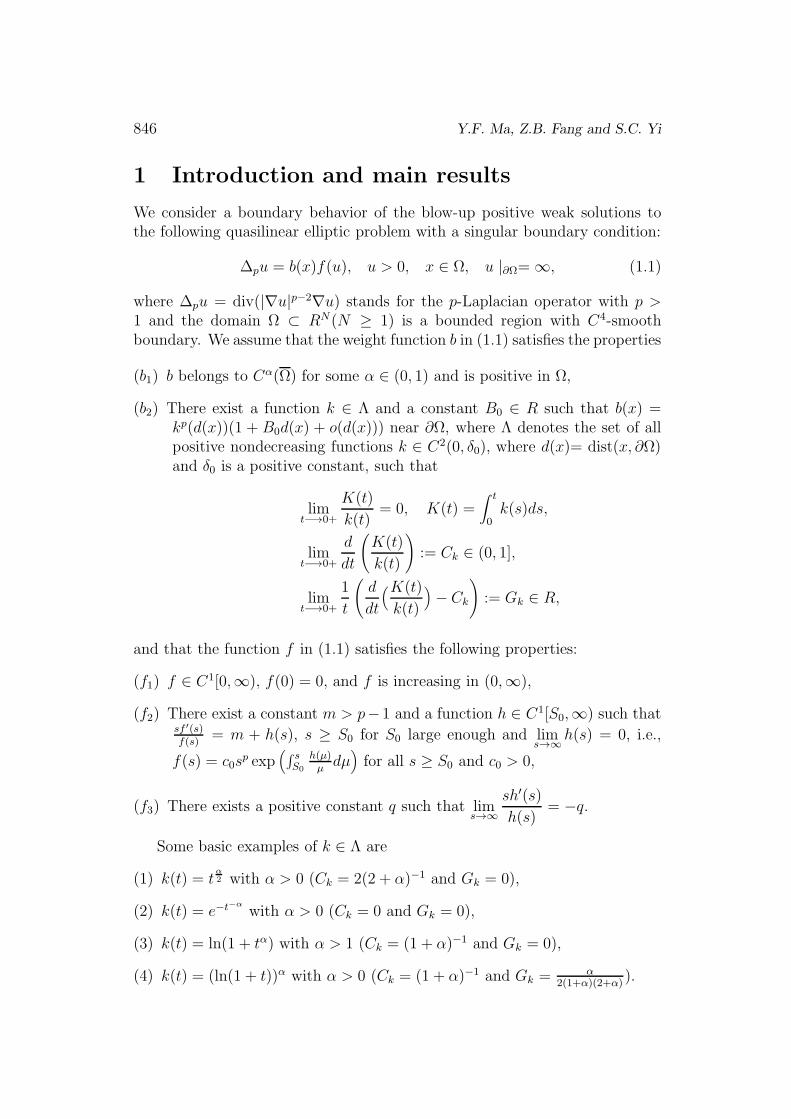
We consider a boundary behavior of the blow-up positive weak solutions tothe following quasilinear elliptic problem with a singular boundary condition:
∆pu = b(x)f(u), u > 0, x ∈ Ω, u |∂Ω= ∞, (1.1)
where ∆pu = div(|∇u|p−2∇u) stands for the p-Laplacian operator with p >1 and the domain Ω ⊂ RN(N ≥ 1) is a bounded region with C4-smoothboundary. We assume that the weight function b in (1.1) satisfies the properties
(b1) b belongs to Cα(Ω) for some α ∈ (0, 1) and is positive in Ω,
(b2) There exist a function k ∈ Λ and a constant B0 ∈ R such that b(x) =kp(d(x))(1 + B0d(x) + o(d(x))) near ∂Ω, where Λ denotes the set of allpositive nondecreasing functions k ∈ C2(0, δ0), where d(x)= dist(x, ∂Ω)and δ0 is a positive constant, such that
limt−→0+
K(t)
k(t)= 0, K(t) =
∫ t
0k(s)ds,
limt−→0+
d
dt
(K(t)
k(t)
):= Ck ∈ (0, 1],
limt−→0+
1
t
(d
dt
(K(t)
k(t)
)− Ck
):= Gk ∈ R,
and that the function f in (1.1) satisfies the following properties:
(f1) f ∈ C1[0,∞), f(0) = 0, and f is increasing in (0,∞),
(f2) There exist a constant m > p−1 and a function h ∈ C1[S0,∞) such thatsf ′(s)f(s)
= m + h(s), s ≥ S0 for S0 large enough and lims→∞
h(s) = 0, i.e.,
f(s) = c0sp exp
(∫ sS0
h(µ)µ
dµ)for all s ≥ S0 and c0 > 0,
(f3) There exists a positive constant q such that lims→∞
sh′(s)
h(s)= −q.
Some basic examples of k ∈ Λ are
(1) k(t) = tα2 with α > 0 (Ck = 2(2 + α)−1 and Gk = 0),
(2) k(t) = e−t−α
with α > 0 (Ck = 0 and Gk = 0),
(3) k(t) = ln(1 + tα) with α > 1 (Ck = (1 + α)−1 and Gk = 0),
(4) k(t) = (ln(1 + t))α with α > 0 (Ck = (1 + α)−1 and Gk = α2(1+α)(2+α)
).

A second expansion of positive large solutions for quasilinear elliptic equations 847
By a solution of (1.1), we mean there exists a function u ∈ W 1,ploc (Ω)
⋂L∞loc(Ω)
such that ∆pu = b(x)f(u) in the weak sense and u satisfies the singular bound-ary condition, i.e., u(x) → ∞ as d(x)=dist(x, ∂Ω) → 0. This solution is alsocalled a large solution, an explosive solution or a boundary blow-up solution.
Problem (1.1) appears in the study of a steady-state for the non-Newtonianfluids through porous media, combustion theory, and the turbulent flow ofa gas in porous media. In the non-Newtonian fluid theory, the quantity pcharacterizes the media. Media with p > 2 are called dilatant fluids and thosewith p < 2 are called pseudo plastics. If p = 2, they are Newtonian fluids. Thep-Laplacian operator also appears in the study of torsional creep; for example,elastic for p = 2 and plastic for p < 2, see [1], flow through porous media(p = 3
2, see [2]) or glacial sliding (p ∈ (1, 4
3], see [3]).
Problem (1.1) with p = 2, N = 2, b(x) = 1, and f(u) = eu was firstconsidered by Bieberbach [4] in early 1916, and the author showed that thereexists a unique solution u ∈ C2(Ω) such that u(x) − log(d−2(x)) = O(1) asd(x) → 0 in two-dimensional space. Problems of this type arise frequentlyin Riemannian geometry. More precisely, if a Riemannian metric of the form|ds|2 = e2u(x)|dx|2 has the constant Gaussian curvature −b2, then u = b2e2u.Many scholars showed existence and uniqueness of blow-up solutions and gaveaccurate estimates and more perfect results on the boundary behaviors ofthe large solutions to the semilinear elliptic, logistic, and elliptic equations,see [5-13] and references therein. Recently, when p > 1 and the functionsb and f satisfy some proper conditions, many researchers proved existenceand uniqueness of large solutions to the equations and gave blow up rates ofthe solutions by using the perturbed, the lower and upper solutions methodsand radial solutions and by constructing comparison functions, see [14-21] andreferences therein.
Cirstea and Radulescu [8,9] first adopted the Karamata regular variationtheory to study the boundary blow-up problem of elliptic equations and openedup a new efficient method which can deal with the uniqueness of boundaryblow-up solutions and boundary behavior in a general framework that removesprevious restrictions, and they expanded the existing results. In particular,this setting becomes a powerful tool in describing the asymptotic behavior ofsolutions for large classes of nonlinear elliptic equations, and singular solutionswith blow-up boundary and stationary problems with either degenerate orsingular nonlinearity as well. For many researches used the methods to dealwith elliptic problems, see [7-13, 21] and references therein. Recently, Zhangand Huang et al. [11,13] established the second expansion of large solutionsfor problem (1.1) when p = 2 by using the Karamata regular variation theory,the perturbed, and the lower and upper solutions methods. Huang et al. [21]investigated the asymptotic behavior of boundary blow-up solutions to thequasilinear elliptic problem (1.1), when the weight function b is nonnegative

848 Y.F. Ma, Z.B. Fang and S.C. Yi
and nontrivial, which may vanish on the boundary, and the nonlinear functionf is a Γ-varying function at infinity, whose variation at infinity is not regular.
Motivated by the mentioned works above, we will analyze an influence ofmean curvature in the boundary behavior of solutions to problem (1.1), wherethe weight b covers a broad class of functions and the absorption f covers alarge class of Keller-Osserman type nonlinearities; that is, we will establish asecond expansion of the singular solutions near the boundary via the Karamatatheory.
Our more detailed results can be summarized as follows:
Theorem 1.1 Suppose that f satisfies (f1)-(f3) and that b satisfies (b1)and (b2) with Ck ∈ (0, 1). If q is a constant in hypothesis (f3) such that
q ∈(m+1−p
p, m+ 1
), then the unique solution of problem (1.1) can be written
as
u(x) = ξ0φ(K(d(x)))(1+C1d(x)+C2H(x)d(x)+o(d(x))
)as d(x) → 0, (1.2)
where for all x ∈ Ω in a neighborhood of ∂Ω, x ∈ ∂Ω is the unique point suchthat d(x) = |x− x| and H(x) is the mean curvature of ∂Ω at the point x, andφ is uniquely defined by
∫ ∞
φ(t)(p′f(µ))−
1pdµ = t,
1
p′+
1
p= 1, ∀t > 0, (1.3)
and
ξ0 =
((p− 1)
p+ Ck(m+ 1− p)
m+ 1
) 1m+1−p
, (1.4)
C1 =(m+ 1− p)Gk − B0(p+ (m+ 1− p)Ck)
((m+ 1− p)Ck + p)(m− 1), (1.5)
C2 =(N − 1)(m+ 1− p)Ck
(m+ 1− p)Ck +m2 +m− p. (1.6)
For the following theorem, we now give an additional condition on thefunction f as follows:
(f4) There exist constants m > p−1 and c0 > 0 and a function h1 ∈ C1[S0,∞)such that f(s) = c0s
m(1+h1(s)), where s ≥ S0 for S0 large enough, andlims→∞
h1(s) = 0.
Theorem 1.2 Suppose that b satisfies (b1) and (b2) and that f satisfies (f1)
and (f4). If h1 is a function in hypothesis (f4) such that lims→∞
sh′1(s)
h1(s)= −q1

A second expansion of positive large solutions for quasilinear elliptic equations 849
and 2q1 > (p− 1)Ck, then the unique solution of problem (1.1) can be writtenas
u(x) = ξ1(K(d(x)))−p
m+1−p
(1 + C3d(x) + C4H(x)d(x) + o(d(x))
)as d(x) → 0,
(1.2)where for all x ∈ Ω in a neighborhood of ∂Ω, x ∈ ∂Ω is the unique point suchthat d(x) = |x− x| and H(x) is the mean curvature of ∂Ω at the point x, and
ξ1 =
((p− 1)pp−1(p+ Ck(m+ 1− p))
c0(m+ 1− p)p
) 1m+1−p
, (1.7)
C3 =(m+ 1− p)Gk − B0(p+ (m+ 1− p)Ck)
((m+ 1− p)(m+ 1)Ck)− p(m− 1), (1.8)
C4 =(N − 1)(m+ 1− p)Ck
(m+ 1− p)(m+ 1)Ck − p(m− 1). (1.9)
Remark 1.1 By a direct calculation, one can see that h(s) =s(1+h′
1(s))
1+h1(s)for
s ∈ [S0,∞). Moreover, it will be seen that q = q1 in Section 2.
Remark 1.2 From Lemma 2.13 given in Section 2, one can see that thefunction f in (1.1) satisfies the Keller-Osserman condition, and hence, thesolution for problem (1.1) exists, see [17].
Our paper is organized as follows: In Section 2, some notions and resultsfrom regular variation theory are given. Theorems 1 and 2 will be proved inSections 3 and 4, respectively.
2 Preliminary results
2.1 Properties of regularly varying function
The Karamata regular variation theory was established by Karamata in 1930,which is a basic tool in the stochastic process, and in 1970 Haan improved theresults, which have been applied to the stochastic process, the analytical func-tion theory, integral functions, integral transforms, and asymptotic estimationof integral sequences, see [22-24].
We present some definitions and basic properties of regularly varying func-tions.
Definition 2.1 A positive measurable function f defined on [a,∞) is saidto be regularly varying at infinity with index ρ, written as f ∈ RVρ, if for eachξ > 0 and some ρ ∈ R
limt→∞
f(ξt)
f(t)= ξρ, (2.1)

850 Y.F. Ma, Z.B. Fang and S.C. Yi
where a is a positive constant. In particular, when ρ = 0, the function f issaid to be slowly varying at infinity.
Clearly, if f ∈ RVρ, then the function L(s) := f(s)sρ
is slowly varying atinfinity.
Definition 2.2 A positive measurable function f defined on [a,∞) is saidto be rapidly varying at infinity if for each ρ > 1
lims→∞
f(s)
sρ= ∞, (2.2)
where a is a positive constant.
Some basic examples of slowly varying functions at infinity are
(1) every positive measurable function on [a,∞) which has a positive limit atinfinity,
(2) (ln t)s and (ln(ln t))s for s ∈ R,
(3) e(ln t)s for 0 < s < 1,
and some basic examples of rapidly varying functions at infinity are
(1) et and eet
for t ∈ R,
(2) ee(ln t)s
, eets
, and eets
for s > 0,
(3) tγe(ln t)q and (ln t)γe(ln t)q , where q and γ > 1,
(4) (ln t)γetq
and tγetγ
, where q > 0 and γ ∈ R.
Definition 2.3 We say that a positive measurable function g defined on(0, a) is regularly varying at zero with index σ, written as g ∈ RV Zσ, if themapping t 7→ g(1
t) belongs to RV−σ, where a > 0 is a constant. Similarly,
a function g is said to be rapidly varying at zero if the mapping t 7→ g(1t) is
rapidly varying at infinity.
Proposition 2.4 (Uniform Convergence Theorem)If f ∈ RVρ, then (2.1) holds uniformly for ξ ∈ [c1, c2] with 0 < c1 < c2.Moreover, if ρ < 0, then the uniform convergence holds on all intervals (a1,∞)with a1 > 0, and if ρ > 0 and f is bounded on (0, a1] for all a1 > 0, then theuniform convergence holds on all intervals (0, a1].

A second expansion of positive large solutions for quasilinear elliptic equations 851
Definition 2.5 A function f defined on (a,∞) is said to be normalizedregularly varying at infinity with index ρ, written as f ∈ NRVρ, if it is acontinuously differentiable function such that
lims→∞
sf ′(s)
f(s)= ρ.
When the index ρ = 0, the function f is said to be normalized slowly varyingat infinity.
Definition 2.6 A function g is said to be normalized regularly varying atzero with index σ, written as g ∈ NRV Zσ, if the mapping t 7→ g(1
t) belongs to
NRV−σ.
A function f ∈ RVρ belongs to NRVρ if and only if
f ∈ C1[a1,∞) for some a1 > 0 and lims→∞
sf ′(s)
f(s)= ρ.
Proposition 2.7 (Representation Theorem)A function L is slowly varying at infinity if and only if L can be written as
L(s) = ϕ(s) exp
(∫ s
a1
y(t)
tdt
), s ≥ a1, (2.3)
for some a1 > 0, where the functions ϕ and y are measurable, and y(s) → 0and ϕ(s) → c0 with c0 > 0 as s → ∞.
The function
L(s) := c0 exp
(∫ s
a1
y(t)
tdt
), s ≥ a1, (2.4)
is normalized slowly varying at infinity and
f(s) := c0sρL(s), s ≥ a1, (2.5)
is a normalized regularly varying function at infinity with index ρ.
Proposition 2.8 If the functions L1 and L2 are slowly varying at infinity,then
(1) Lσ with σ ∈ R, c1L+ c2L1, and L L1 are also slowly varying at infinity,where c1 and c2 are nonnegative constants such that c1 + c2 > 0 andL1(t) → ∞ as t → ∞,
(2) for all θ > 0 we have tθL(t) → ∞ and t−θL(t) → 0 as t → ∞,

852 Y.F. Ma, Z.B. Fang and S.C. Yi
(3) for all ρ ∈ R we have ln(L(t))ln t
→ 0 and ln(tρL(t))ln t
→ ρ as t → ∞.
Proposition 2.9 If f1 ∈ RVρ1 and f2 ∈ RVρ2 with limt→∞ f2(t) = ∞, thenf1 f2 ∈ RVρ1ρ2.
Proposition 2.10 (Asymptotic Behavior)If a function L is slowly varying at infinity, then for all a ≥ 0 we have
(1)∫ ta s
βL(s)ds ∼= (β + 1)−1t1+βL(t) for β > −1,
(2)∫∞t sβL(s)ds ∼= (−β − 1)−1t1+βL(t) for β < −1,
as t → ∞.
Proposition 2.11 (Asymptotic Behavior)If a function H is slowly varying at infinity, then for all a > 0 we have
(1)∫ t0 s
βH(s)ds ∼= (β + 1)−1t1+βH(t) for β > −1,
(2)∫∞t sβH(s)ds ∼= (−β − 1)−1t1+βH(t) for β < −1,
as t → 0+.
2.2 Auxiliary results
In this section, we will give some auxiliary results, which will be used in theproofs of Theorems 1 and 2.
Lemma 2.12 (cf. [10])If k ∈ Λ, then we have
(1) limt→0+
K(t)
k(t)= 0 and lim
t→0+
tk(t)
K(t)= C−1
k , i.e., K ∈ NRV ZC−1k,
(2) limt→0+
tk′(t)
k(t)=
1− Ck
Ck
, i.e., K ∈ NRV Z 1−CkCk
, and limt→0+
K(t)k′(t)
k2(t)= 1−Ck,
(3) limt→0+
1
t
(K(t)k′(t)
k2(t)− (1− Ck)
)= −Gk.
Set
Θ(t) =∫ ∞
t
ds
(p′F (s))1p
, t > 0. (2.6)
We then have
Θ′(t) = −1
(p′F (t))1p
, t > 0. (2.7)
A second expansion of positive large solutions for quasilinear elliptic equations 853
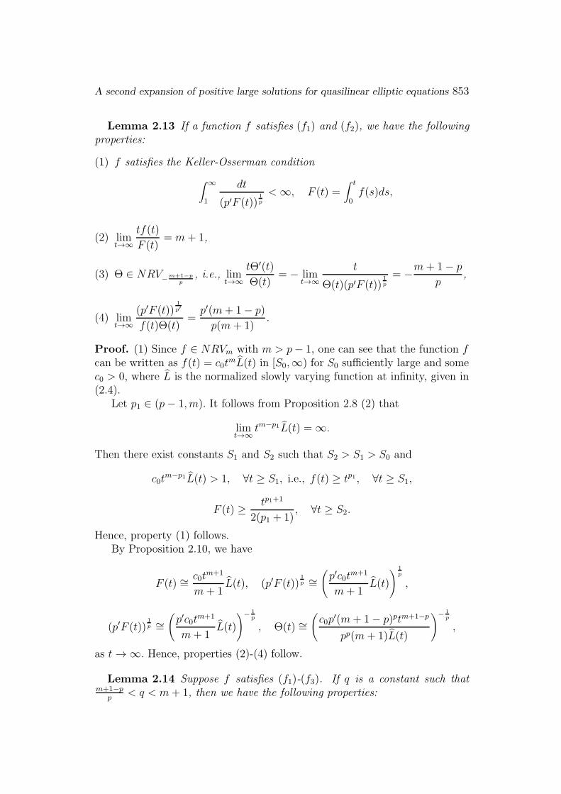
Lemma 2.13 If a function f satisfies (f1) and (f2), we have the followingproperties:
(1) f satisfies the Keller-Osserman condition
∫ ∞
1
dt
(p′F (t))1p
< ∞, F (t) =∫ t
0f(s)ds,
(2) limt→∞
tf(t)
F (t)= m+ 1,
(3) Θ ∈ NRV−
m+1−pp
, i.e., limt→∞
tΘ′(t)
Θ(t)= − lim
t→∞
t
Θ(t)(p′F (t))1p
= −m+ 1− p
p,
(4) limt→∞
(p′F (t))1p′
f(t)Θ(t)=
p′(m+ 1− p)
p(m+ 1).
Proof. (1) Since f ∈ NRVm with m > p− 1, one can see that the function fcan be written as f(t) = c0t
mL(t) in [S0,∞) for S0 sufficiently large and somec0 > 0, where L is the normalized slowly varying function at infinity, given in(2.4).
Let p1 ∈ (p− 1, m). It follows from Proposition 2.8 (2) that
limt→∞
tm−p1L(t) = ∞.
Then there exist constants S1 and S2 such that S2 > S1 > S0 and
c0tm−p1L(t) > 1, ∀t ≥ S1, i.e., f(t) ≥ tp1 , ∀t ≥ S1,
F (t) ≥tp1+1
2(p1 + 1), ∀t ≥ S2.
Hence, property (1) follows.By Proposition 2.10, we have
F (t) ∼=c0t
m+1
m+ 1L(t), (p′F (t))
1p ∼=
(p′c0t
m+1
m+ 1L(t)
) 1p
,
(p′F (t))1p ∼=
(p′c0t
m+1
m+ 1L(t)
)− 1p
, Θ(t) ∼=
(c0p
′(m+ 1− p)ptm+1−p
pp(m+ 1)L(t)
)− 1p
,
as t → ∞. Hence, properties (2)-(4) follow.
Lemma 2.14 Suppose f satisfies (f1)-(f3). If q is a constant such thatm+1−p
p< q < m+ 1, then we have the following properties:

854 Y.F. Ma, Z.B. Fang and S.C. Yi
(1) limt→∞
tf ′(t)f(t)
−m
Θ(t)= 0,
(2) limt→∞
F (t)tf(t)
− 1m+1
Θ(t)= 0,
(3) limt→∞
(p′F (t))1p′
f(t)Θ(t)− p′(m+1−p)
p(m+1)
Θ(t)= 0,
(4) limt→∞
(f(ξ0t))
ξp−10 f(t)
− ξm+1−p0
Θ(t)= 0, ξ0 > 0.
Proof. We only prove (3) and (4).
(3) limt→∞
(p′F (t))1p′
f(t)Θ(t)− p′(m+1−p)
p(m+1)
Θ(t)
= limt→∞
(p′F (t))1p′
f(t)Θ(t)− p′(m+1−p)
p(m+1)
Θ2Θ(t)(t)
= limt→∞
p′ (F (t))tf(t)
· tf ′(t)f(t)
− p′mp(m+1)
2Θ(t)
= limt→∞
p′((F (t))tf(t)
− 1m+1
)·(tf ′(t)f(t)
−m)+ p′
m+1
(tf ′(t)f(t)
−m)+mp′
(F (t)tf(t)
− 1m+1
)
2Θ(t)= 0.
(4) When ξ0 = 1, the result is obvious. Let ξ0 6= 1. By (f2), one can seethat
f(ξ0t)
ξp−10 f(t)
− ξm+1−p0 = ξm+1−p
0
(exp
( ∫ ξ0t
t
h(s)
sds)− 1
).
By Proposition 2.8, it can be seen that
limt→∞
h(ts)
s= 0 and lim
t→∞
h(ts)
sh(t)= s−q−1,
uniformly for s ∈ [1, ξ0] or [ξ0, 1].Therefore, we can obtain the equalities
limt→∞
∫ ξ0t
t
h(s)
sds = lim
t→∞
∫ ξ0
1
h(ts)
sds = 0,
and
limt→∞
∫ ξ0
1
h(ts)
sh(t)ds = lim
t→∞
∫ ξ0
1s−q−1ds = q−1(1− ξ−q
0 ),

A second expansion of positive large solutions for quasilinear elliptic equations 855
since er − 1 ∼= r as r → 0, which lead to
f(ξ0t)
ξp−10 f(t)
− ξm+1−p0 = ξm+1−p
0 limt→∞
∫ ξ01
h(ts)s
ds
Θ(t)
= ξm+1−p0 lim
t→∞
h(t)
Θ(t)· limt→∞
∫ ξ0
1
h(ts)
sh(t)ds = 0.
This completes the proof.
Lemma 2.15 Under the hypotheses in Theorem 1.1, if φ is a solution tothe equation ∫ ∞
φ(t)(p′F (t))−
1p = t, ∀t > 0,
then we have the following properties:
(1) −φ′(t) =(p′F (φ(t))
) 1p , φ(t) > 0, t > 0, φ(0) := lim
t→0+φ(t) = ∞, and
φ′′(t) = (p′ − 1)(p′F (φ(t))
) 2−p
p f(φ(t)),
(2) limt→0+
tφ′(t)
φ(t)= −
p
m+ 1− p,
(3) limt→0+
φ′(t)
tφ′′(t)= −
m+ 1− p
m+ 1,
(4) limt→0+
φ(t)
t2φ′′(t)=
(m+ 1− p)2
p(m+ 1),
(5) limt→0+
1
t
(φ′(t)
tφ′′(t)+
m+ 1− p
m+ 1
)= 0,
(6) limt→0+
1
t
(1 +
φ′(K(t))
K(t)φ′′(K(t))·K(t)k′(t)
k2(t)−
1
p− 1
f(ξ0φ(K(t)))
ξp−10 f(φ(K(t)))
)=
m+ 1− p
m+ 1Gk,
for all k ∈ Λ.
Proof. (1) Property (1) easily follows by the definition of φ and a directcalculation.
To show properties (2)-(5), set u = φ(t). By L’Hospital’s rule and Lemma2.14, one can obtain (2)-(5), i.e.,
limt→0+
tφ′(t)
φ(t)= − lim
t→0+
t(p′F (φ(t)))1p
φ(t)
856 Y.F. Ma, Z.B. Fang and S.C. Yi
= − limu→∞
(p′F (u))1p∫∞u (p′F (s))−
1pds
u= −
p
m+ 1− p,
limt→0+
φ′(t)
tφ′′(t)= − lim
t→0+
(p′F (φ(t)))1p
tφ(t)= − lim
u→∞
(p′F (u))1p
(p′ − 1)f(u)Θ(u)= −
m+ 1− p
m+ 1,
limt→0+
φ(t)
t2φ′′(t)= lim
t→0+
φ(t)
tφ′(t)· limt→0+
φ′(t)
tφ′′(t)=
m+ 1− p
p·m+ 1− p
m+ 1=
(m+ 1− p)2
p(m+ 1),
limt→0+
1
t
(φ′(t)
tφ′′(t)+
m+ 1− p
m+ 1
)= − lim
u→∞
(p′F (u))1p′
(p′−1)f(u)Θ(u)− m+1−p
m+1
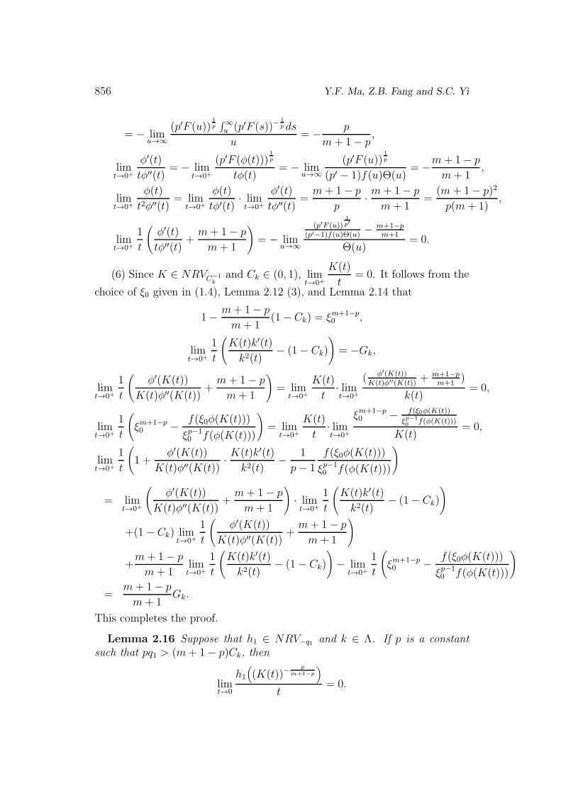
Θ(u)= 0.
(6) Since K ∈ NRVC−1k
and Ck ∈ (0, 1), limt→0+
K(t)
t= 0. It follows from the
choice of ξ0 given in (1.4), Lemma 2.12 (3), and Lemma 2.14 that
1−m+ 1− p
m+ 1(1− Ck) = ξm+1−p
0 ,
limt→0+
1
t
(K(t)k′(t)
k2(t)− (1− Ck)
)= −Gk,
limt→0+
1
t
(φ′(K(t))
K(t)φ′′(K(t))+
m+ 1− p
m+ 1
)= lim
t→0+
K(t)
t· limt→0+
( φ′(K(t))K(t)φ′′(K(t))
+ m+1−pm+1
)
k(t)= 0,
limt→0+
1
t
(ξm+1−p0 −
f(ξ0φ(K(t)))
ξp−10 f(φ(K(t)))
)= lim
t→0+
K(t)
t· limt→0+
ξm+1−p0 − f(ξ0φ(K(t))
ξp−10 f(φ(K(t)))
K(t)= 0,
limt→0+
1
t
(1 +
φ′(K(t))
K(t)φ′′(K(t))·K(t)k′(t)
k2(t)−
1
p− 1
f(ξ0φ(K(t)))
ξp−10 f(φ(K(t)))
)
= limt→0+
(φ′(K(t))
K(t)φ′′(K(t))+
m+ 1− p
m+ 1
)· limt→0+
1
t
(K(t)k′(t)
k2(t)− (1− Ck)
)
+(1− Ck) limt→0+
1
t
(φ′(K(t))
K(t)φ′′(K(t))+
m+ 1− p
m+ 1
)
+m+ 1− p
m+ 1limt→0+
1
t
(K(t)k′(t)
k2(t)− (1− Ck)
)− lim
t→0+
1
t
(ξm+1−p0 −
f(ξ0φ(K(t)))
ξp−10 f(φ(K(t)))
)
=m+ 1− p
m+ 1Gk.
This completes the proof.
Lemma 2.16 Suppose that h1 ∈ NRV−q1 and k ∈ Λ. If p is a constantsuch that pq1 > (m+ 1− p)Ck, then
limt→0
h1
((K(t))−
p
m+1−p
)
t= 0.

A second expansion of positive large solutions for quasilinear elliptic equations 857
Proof. By Lemma 2.12, we see that K ∈ NRVC−1k. It follows from Propo-
sition 2.9 that h1 K−p
m+1−p ∈ NRV Z pq1(m+1−p)Ck
. Hence, the result follows by
Proposition 2.8 (2), since pq1(m+1−p)Ck
> 1.
3 Proof of Theorem 1.1
In this section, we will prove Theorem 1.1. The upper and lower solutionsmethod is an important tool in proving the theorem, and so, establishing acomparison principle is very important. Therefore, we first give a comparisonprinciple, shown in [15], for general quasilinear elliptic equations.
Lemma 3.1 (cf. [15])Suppose that D is a bounded domain in RN and that a(x) and β(x) are con-tinuous functions on D such that ||a||L∞(D) < ∞ and β(x) is nonnegativeand nontrivial in D. If u1 and u2 ∈ C1(D) are positive in D and satisfy thefollowing inequalities in the sense of distributions:
−∆pu1 − a(x)up−11 − β(x)g(u1) ≥ 0 ≥ −∆pu2 − a(x)up−1
2 − β(x)g(u2),
limd(x,∂Ω)→0
(up−12 − up−1
1
)≤ 0,
where g ∈ C0([0,∞)) and g(s)sp−1 is increasing on the interval
(infD(u1, u2), sup
D
(u1, u2)),
then we have the inequality u1 ≥ u2 in D.
Fix ǫ > 0, and for all δ > 0 we define a set Ωδ = x ∈ Ω : 0 < d(x) < δ.Since ∂Ω is C4-smooth, we can choose δ1 ∈ (0, δ0) such that d ∈ C4(Ωδ1) and
|∇d(x)| = 1, d(x) = −(N − 1)H(x)d(x) + o(1), ∀x ∈ Ωδ1 . (3.1)
Let a0 ∈(0,min1, m
2+m−pp
)and let
w± = ξ0φ(K(d(x)))(1 + (C1 ± ε)d(x) + C2H(x)d(x)
), x ∈ Ωδ1 .
By the Lagrange mean value theorem, one can see that there exist constantsλ± ∈ (0, 1) such that
f(w±(x)) = f(ξ0φ(K(d(x))))+ξ0φ(K(d(x)))f ′(φ±(d(x)))((C1±ǫ)d(x)+C2H(x)d(x)
),
for all x ∈ Ωδ1 , where
φ±(d(x)) = ξ0φ(K(d(x)))(1 + λ±(C1 ± ε)d(x) + C2H(x)d(x)
).
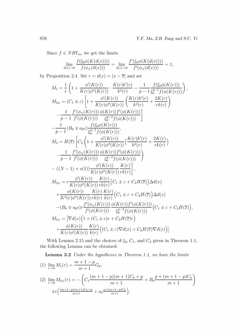
858 Y.F. Ma, Z.B. Fang and S.C. Yi
Since f ∈ NRVm, we get the limits
limd(x)→0
f(ξ0φ(K(d(x))))
f(φ±(d(x)))= lim
d(x)→0
f ′(ξ0φ(K(d(x))))
f ′(φ±(d(x)))= 1,
by Proposition 2.4. Set r = d(x) = |x− x| and set
M1 =1
r
(1 +
φ′(K(r))
K(r)φ′′(K(r))·K(r)k′(r)
k2(r)−
1
p− 1
f(ξ0φ(K(r)))
ξp−10 f(φ(K(r)))
),
M2± = (C1 ± ε)
[1 +
φ′(K(r))
K(r)φ′′(K(r))
(K(r)k′(r)
k2(r)+
2K(r)
rk(r)
)
−1
p− 1
f ′(φ±(K(r)))
f ′(φ(K(r)))
φ(K(r))f ′(φ(K(r)))
ξp−20 f(φ(K(r)))
]
−1
p− 1(B0 ∓ a0ǫ)
f(ξ0φ(K(r)))
ξp−10 f(φ(K(r)))
,
M3 = H(x)
[C2
(1 +
φ′(K(r))
K(r)φ′′(K(r))
(K(r)k′(r)
k2(r)+
2K(r)
rk(r)
)
−1
p− 1
f ′(φ±(K(r)))
f ′(φ(K(r)))
φ(K(r))f ′(φ(K(r)))
ξp−20 f(φ(K(r)))
)
− ((N − 1) + o(1))φ′(K(r))
K(r)φ′′(K(r))
K(r)
rk(r)
],
M4± = rφ′(K(r))
K(r)φ′′(K(r))
K(r)
rk(r)
(C1 ± ε+ C2H(x)
)∆d(x)
+φ(K(r))
K2(r)φ′′(K(r))
K(r)
rk(r)
K(r)
k(r)
(C1 ± ε+ C2H(x)
)∆d(x)
−(B0 ∓ a0ǫ)rf ′(φ±(K(r)))
f ′(φ(K(r)))
φ(K(r))f ′(φ(K(r)))
ξp−20 f(φ(K(r)))
(C1 ± ε+ C2H(x)
),
M5± =∣∣∣∇d(x)
(1 + (C1 ± ǫ)r + C2H(x)r
)
+φ(K(r))
K(r)φ′(K(r))
K(r)
k(r)
((C1 ± ε)∇d(x) + C2H(x)∇d(x)
)∣∣∣.
With Lemma 2.15 and the choices of ξ0, C1, and C2 given in Theorem 1.1,the following Lemma can be obtained:
Lemma 3.2 Under the hypotheses in Theorem 1.1, we have the limits
(1) limr→0
M1(r) =m+ 1− p
m+ 1Gk,
(2) limr→0
M2±(r) = −
(C1
(m+ 1− p)(m+ 1)Ck + p
m+ 1+B0
p+ (m+ 1− p)Ck
m+ 1
)
∓ǫ((m+1−p)(m+1)Ck+p
m+1+ a0
p+(m+1−p)Ck
m+1
),
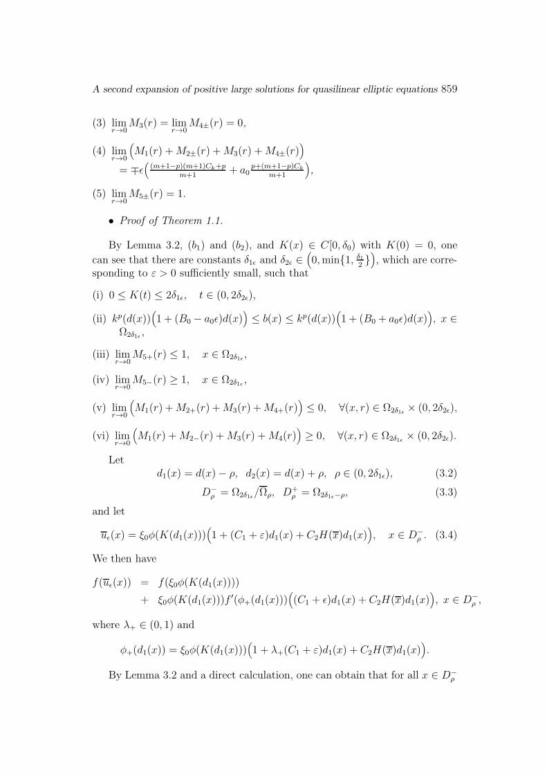
A second expansion of positive large solutions for quasilinear elliptic equations 859
(3) limr→0
M3(r) = limr→0
M4±(r) = 0,
(4) limr→0
(M1(r) +M2±(r) +M3(r) +M4±(r)
)
= ∓ǫ((m+1−p)(m+1)Ck+p
m+1+ a0
p+(m+1−p)Ck
m+1
),
(5) limr→0
M5±(r) = 1.
• Proof of Theorem 1.1.
By Lemma 3.2, (b1) and (b2), and K(x) ∈ C[0, δ0) with K(0) = 0, one
can see that there are constants δ1ǫ and δ2ǫ ∈(0,min1, δ1
2), which are corre-
sponding to ε > 0 sufficiently small, such that
(i) 0 ≤ K(t) ≤ 2δ1ǫ, t ∈ (0, 2δ2ǫ),
(ii) kp(d(x))(1 + (B0 − a0ǫ)d(x)
)≤ b(x) ≤ kp(d(x))
(1 + (B0 + a0ǫ)d(x)
), x ∈
Ω2δ1ǫ ,
(iii) limr→0
M5+(r) ≤ 1, x ∈ Ω2δ1ǫ ,
(iv) limr→0
M5−(r) ≥ 1, x ∈ Ω2δ1ǫ ,
(v) limr→0
(M1(r) +M2+(r) +M3(r) +M4+(r)
)≤ 0, ∀(x, r) ∈ Ω2δ1ǫ × (0, 2δ2ǫ),
(vi) limr→0
(M1(r) +M2−(r) +M3(r) +M4(r)
)≥ 0, ∀(x, r) ∈ Ω2δ1ǫ × (0, 2δ2ǫ).
Letd1(x) = d(x)− ρ, d2(x) = d(x) + ρ, ρ ∈ (0, 2δ1ǫ), (3.2)
D−ρ = Ω2δ1ǫ/Ωρ, D+
ρ = Ω2δ1ǫ−ρ, (3.3)
and let
uǫ(x) = ξ0φ(K(d1(x)))(1 + (C1 + ε)d1(x) + C2H(x)d1(x)
), x ∈ D−
ρ . (3.4)
We then have
f(uǫ(x)) = f(ξ0φ(K(d1(x))))
+ ξ0φ(K(d1(x)))f′(φ+(d1(x)))
((C1 + ǫ)d1(x) + C2H(x)d1(x)
), x ∈ D−
ρ ,
where λ+ ∈ (0, 1) and
φ+(d1(x)) = ξ0φ(K(d1(x)))(1 + λ+(C1 + ε)d1(x) + C2H(x)d1(x)
).
By Lemma 3.2 and a direct calculation, one can obtain that for all x ∈ D−ρ

860 Y.F. Ma, Z.B. Fang and S.C. Yi
puε(x)− kp(d1(x))(1 + (B0 − ε)d1(x)
)f(uǫ(x))
= (p− 1)ξp−10
∣∣∣φ′(K(d1(x)))∣∣∣p−2∣∣∣kp−2(d1(x))
∣∣∣∣∣∣∇d(x)
(1 + (C1 + ε)d1(x) + C2H(x)d1(x)
)
+φ(K(d1(x)))
K(d1(x))φ′′(K(d1(x)))·K(d1(x))
k(d1(x))
((C1 + ε)∇d(x) + C2H(x)∇d(x)
)∣∣∣p−2
·
[φ′′(K(d1(x)))k
2(d1(x))(1 + (C1 + ε)d1(x) + C2H(x)d1(x)
)
+φ′(K(d1(x)))k′(d1(x))
(1 + (C1 + ε)d1(x) + C2H(x)d1(x)
)
+φ′(K(d1(x)))k(d1(x))∆d(x)(1 + (C1 + ε)d1(x) + C2H(x)d1(x)
)
+2φ′(K(d1(x)))k(d1(x))∇d(x)((C1 + ε)∇d(x) + C2H(x)∇d(x)
)
+ φ(K(d1(x)))((C1 + ε)d(x) + C2H(x)d(x)
)]
− kp(d1(x))(1 + (B0 − ε)d1(x)
)[f(ξ0φ(K(d1(x))))
+ ξ0φ(K(d1(x)))f′(φ+(d1(x)))
((C1 + ǫ)d1(x) + C2H(x)d1(x)
)]
= (p− 1)ξp−10
∣∣∣φ′(K(d1(x)))∣∣∣p−2
φ′′(K(d1(x)))kp(d1(x))d1(x)M5+(x) ·
(M1(r) +M2+(r) +M3(x) +M4+(x)
)
≤ 0,
where r = d1(x), which implies that uε is an upper solution of equation (1.1)in D−
ρ .By a similar argument, it can be shown that
uǫ(x) = ξ0φ(K(d2(x)))(1 + (C1 − ε)d2(x) + C2H(x)d2(x)
), x ∈ D+
ρ (3.5)
is a lower solution of (1.1) in D+ρ .
Let u be an arbitrary solution of problem (1.1) and let C1(δε) = maxd(x)≥δǫ
u(x).
We then have the inequality
u ≤ C1(δ1ε) + uǫ on ∂D−ρ .
Since φ1 is decreasing, we get the inequalities
uǫ ≤ ξ0φ(K(2δε)) := C2(δε), whenever d(x) = 2δε − ρ,
anduǫ ≤ u+ C2(δε) on ∂D+
ρ .
It follows from (f1) and Lemma 3.1 that
u ≤ C1(δε) + uǫ, x ∈ D−ρ and uǫ ≤ u+ C2(δε), x ∈ D+
ρ .

A second expansion of positive large solutions for quasilinear elliptic equations 861
Hence, letting ρ → 0, we have that for all x ∈ D−ρ ∩D+
ρ ,
1 + (C1 − ǫ)d(x) + C2H(x)d(x)−C2(δǫ)
ξ0φ(K(d(x)))≤
u(x)
ξ0φ(K(d(x))),
and
u(x)
ξ0φ(K(d(x)))≤ 1 + (C1 + ǫ)d(x) + C2H(x)d(x) +
C1(δǫ)
ξ0φ(K(d(x))).
Consequently, we obtain the inequalities
C1 − ǫ+ C2H(x) ≤ lim infd(x)→0
(d(x))−1( u(x)
ξ0φ(K(d(x)))− 1
),
and
lim supd(x)→0
(d(x))−1( u(x)
ξ0φ(K(d(x)))− 1
)≤ C1 + ǫ+ C2H(x).
Letting ǫ → 0 we have the limit
limd(x)→0
(d(x))−1( u(x)
ξ0φ(K(d(x)))− 1
)= C1 + C2H(x).
This completes the proof.
4 Proof of Theorem 1.2
In this section, we will prove Theorem 1.2. To show the result of this theorem,we first introduce a lemma with proof below:
Let a0 ∈(0,min1, m2+m−p
p)and let
w±(x) = ξ1(K(d(x)))−p
m+1−p
(1 + (C3 ± ǫ)d(x) + C4H(x)d(x)
),
where x ∈ Ωδ1 . Then, we get
f(w±(x)) = c0ξm1 (K(d(x)))−
mpm+1−p (1+g1(w±(x)))
(1+m(C3±ǫ)d(x)+mC4H(x)d(x)
),
where x ∈ Ωδ1 .Set r = d(x) = |x− x| and set
M1(r) =1
r
(p(m+ 1)
(m+ 1− p)2−
p
m+ 1− p
K(r)k′(r)
k2(r)
−c0ξ
m+1−p1
p− 1
( p
m+ 1− p
)−(p−2)(1 + g(w±(x)))
),

862 Y.F. Ma, Z.B. Fang and S.C. Yi
M2±(r) = (C3 ± ε)
(p(m+ 1)
(m+ 1− p)2−
p
m+ 1− p
K(r)k′(r)
k2(r)
−2p
m+ 1− p
K(r)
rk(r)−
c0m
p− 1
( p
m+ 1− p
)−(p−2)ξm+1−p1
)
−c0
p− 1
(p
m+ 1− p
)−(p−2)
ξm+1−p1 (B0 ∓ a0ǫ),
M3(r) = H(x)C4
(p(m+ 1)
(m+ 1− p)2−
p
m+ 1− p
K(r)k′(r)
k2(r)
−2p
m+ 1− p
K(r)
rk(r)−
c0m
p− 1
( p
m+ 1− p
)−(p−2)ξm+1−p1
)
−
(p
m+ 1− p
)K(r)
rk(r)d(x),
M4±(r) = −1
p− 1·
p
m+ 1− p
K(r)
k(r)
(C3 ± ε+ C4H(x)
)
+ r
(K(r)
rk(r)
)2 (C3 + ε+ C4H(x)
)d(x)
−c0
p− 1
(p
m+ 1− p
)−(p−2)
ξm+1−p1
((B0 ∓ a0ε)g(w±)(B0 ∓ a0ε)r
+ g(w±(x))(B0 ∓ a0ε)rg(w±(x))(m(C3 ± ε) +mC4H(x))),
M5±(r) = −p
m+ 1− p−d(x)
(1 + C3 ± ε+ C4H(x)
)
+K(d2(x))
k(d2(x))
(C3 ± ε+ C4H(x)
) d(x).
Combining Lemmas 2.12 and 2.16 with the choices of ξ1, C3, and C4 givenin Theorem 1.2, the following lemma can be obtained:
Lemma 4.1 Under the hypotheses given in Theorem 1.2, we have the prop-erties
(1) limr→0
M1 =p
m+ 1− pGk,
(2) limr→0
M2± = −p(C1 ± ε)
((m+ 1− p)(m+ 1)CK − (m− 1)
(m+ 1− p)2
)
− p(B0 ∓ a0ε)(m+ 1− p)CK + p
(m+ 1− p)2,
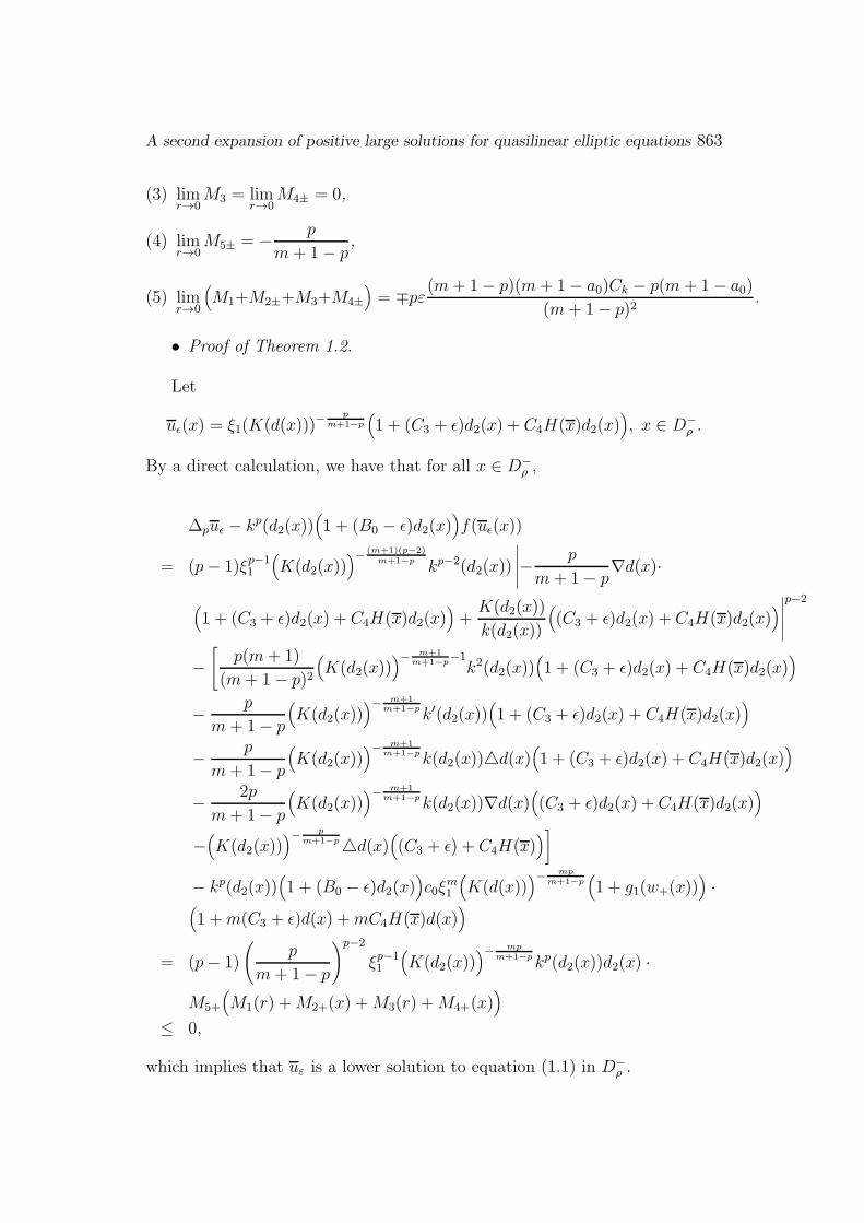
A second expansion of positive large solutions for quasilinear elliptic equations 863
(3) limr→0
M3 = limr→0
M4± = 0,
(4) limr→0
M5± = −p
m+ 1− p,
(5) limr→0
(M1+M2±+M3+M4±
)= ∓pε
(m+ 1− p)(m+ 1− a0)Ck − p(m+ 1− a0)
(m+ 1− p)2.
• Proof of Theorem 1.2.
Let
uǫ(x) = ξ1(K(d(x)))−p
m+1−p
(1 + (C3 + ǫ)d2(x) + C4H(x)d2(x)
), x ∈ D−
ρ .
By a direct calculation, we have that for all x ∈ D−ρ ,
∆puǫ − kp(d2(x))(1 + (B0 − ǫ)d2(x)
)f(uǫ(x))
= (p− 1)ξp−11
(K(d2(x))
)− (m+1)(p−2)m+1−p kp−2(d2(x))
∣∣∣∣∣−p
m+ 1− p∇d(x)·
(1 + (C3 + ǫ)d2(x) + C4H(x)d2(x)
)+
K(d2(x))
k(d2(x))
((C3 + ǫ)d2(x) + C4H(x)d2(x)
)∣∣∣∣∣
p−2
−
[p(m+ 1)
(m+ 1− p)2
(K(d2(x))
)− m+1m+1−p
−1k2(d2(x))
(1 + (C3 + ǫ)d2(x) + C4H(x)d2(x)
)
−p
m+ 1− p
(K(d2(x))
)− m+1m+1−pk′(d2(x))
(1 + (C3 + ǫ)d2(x) + C4H(x)d2(x)
)
−p
m+ 1− p
(K(d2(x))
)− m+1m+1−pk(d2(x))d(x)
(1 + (C3 + ǫ)d2(x) + C4H(x)d2(x)
)
−2p
m+ 1− p
(K(d2(x))
)− m+1m+1−pk(d2(x))∇d(x)
((C3 + ǫ)d2(x) + C4H(x)d2(x)
)
−(K(d2(x))
)− pm+1−pd(x)
((C3 + ǫ) + C4H(x)
)]
− kp(d2(x))(1 + (B0 − ǫ)d2(x)
)c0ξ
m1
(K(d(x))
)− mpm+1−p
(1 + g1(w+(x))
)·
(1 +m(C3 + ǫ)d(x) +mC4H(x)d(x)
)
= (p− 1)
(p
m+ 1− p
)p−2
ξp−11
(K(d2(x))
)− mp
m+1−pkp(d2(x))d2(x) ·
M5+
(M1(r) +M2+(x) +M3(r) +M4+(x)
)
≤ 0,
which implies that uε is a lower solution to equation (1.1) in D−ρ .

864 Y.F. Ma, Z.B. Fang and S.C. Yi
Similarly, it can be shown that
uǫ = ξ1(K(d(x))
)− pm+1−p
(1 + (C3 − ǫ)d2(x) + C4H(x)d2(x)
), x ∈ D+
ρ , (3.5)
is a lower solution of (1.1) in D+ρ .
Letting ρ → 0, we can obtain the inequalities
1 + (C3 − ǫ)d(x) + C4H(x)d(x)−C4(δǫ)
ξ1(K(d(x)))−p
m+1−p
≤u(x)
ξ1(K(d(x)))−p
m+1−p
,
and
u(x)
ξ1(K(d(x)))−p
m+1−p
≤ 1 + (C3 + ǫ)d(x) + C4H(x)d(x) +C4(δǫ)
ξ0(K(d(x)))−p
m+1−p
,
for all x ∈ D−ρ ∩D+
ρ .
Consequently, we can get the inequalities
C3 − ǫ+ C4H(x) ≤ lim infd(x)→0
(d(x))−1
(u(x)
ξ0(K(d(x)))−p
m+1−p
− 1
),
and
lim supd(x)→0
(d(x))−1
(u(x)
ξ0(K(d(x)))−p
m+1−p
− 1
)≤ C3 + ǫ+ C4H(x).
Letting ǫ → 0, we have the limit
limd(x)→0
(d(x))−1
(u(x)
ξ0(K(d(x)))−p
m+1−p
− 1
)= C3 + C4H(x).
This completes the proof.
Acknowledgments
The first two authors were supported by National Science Foundation of Shan-dong Province of China (ZR2012AM018) and Fundamental Research Funds forthe Central Universities (No.201362032), and the research of the third authorwas supported by Changwon National University in 2015. The authors wouldlike to express their sincere gratitude to the anonymous reviewers for theirinsightful and constructive comments.
A second expansion of positive large solutions for quasilinear elliptic equations 865
References
[1] B. Kawohl, On a family of torsional creep problems, J. Reine Angew.Math. 410 (1990) 1-22.
[2] R.E. Showalter, N.J. Walkington, Diffusion of fluid in a fissured mediumwith microstructure, SIAM J. Math. Anal. 22 (1991) 1702-1722.
[3] M.C. P. lissier, M.L. Reynaud, Etude d’ un modele mathematique ecoule-ment de glacier, C. R. Acad. Sci. Paris S6r. I Math. 279 (1974) 531-534.
[4] L. Bieberbach, ∆u = eu und die automorphen Funktionen, Math. Ann.77 (1916) 173-212.
[5] G. Diaz, R. Letelier, Explosive solutions of quasilinear elliptic equations:existence and uniqueness, Nonlinear Anal. 20 (1993) 97-125.
[6] C. Bandle, E. Giarrusso, Boundary blowup for semilinear elliptic equa-tions with nonlinear gradient terms, A. differ. equat. 1 (1996) 133-150.
[7] O. Costin, L. Dupaigne, Boundary blow-up solutions in the unit ball:asymptotics, uniqueness and symmetry, J. differ. equat. 249 (2010) 931-964.
[8] F.C. Cirtea, V. Radulescu, Uniqueness of the blow-up boundary solutionof logistic equations with absorbtion, C. R. Acad. Sci. Paris I 335 (2002)447-452.
[9] F.C. Cirtea, V. Radulescu, Asymptotics for the blow-up boundary solu-tion of the logistic equation with absorption, C. R. Acad. Sci., Paris I 336(2003) 231-236.
[10] Z.J. Zhang, Y.J. Ma, L. Mi, X.H. Li, Blow-up rates of large solutions forelliptic equations, J. differ. equat. 249 (2010) 180-199.
[11] Z.J. Zhang, The second expansion of large solutions for semilinear ellipticequations, Nonlinear Anal. 74 (2011) 3445-3457.
[12] S.B. Huang, Q.Y Tian, S.Z Zhang, J.H. Xi, Z.G. Fan, The exact blow-uprates of large solutions for semilinear elliptic equations, Nonlinear Anal.73 (2010) 3489-3501.
[13] S.B. Huang, Q.Y Tian, S.Z Zhang, J.H. Xi, A second order estimate forblow-up solutions of elliptic equations, Nonlinear Anal. 74 (2011) 2342-2350.
866 Y.F. Ma, Z.B. Fang and S.C. Yi
[14] P.J. Mckenna, T. W. Reichel and W. Walter, Symmetry and multiplic-ity for nonlinear elliptic differential equations with boundary blow up,Nonlinear Anal. 28 (1997) 1213-1225.
[15] Y. Du and Z. M. Guo, Boundary blow up solutions and their applicationsin quasilinear elliptic equations, J. D’Analyse Math. 89 (2003) 277-302.
[16] Q.S. Lu, Z.D. Yang, E. H. Twizell, Existence of entire explosive positivesolutions of quasilinear elliptic equations, Appl. Math. and Comput. 148(2004) 359-372.
[17] Z.M. Guo and J. R. L. Webb, Structure of boundary blow-up solutionsfor quasi-linear elliptic problems II: small and intermediate solutions, J.differ. equat. 211 (2005) 187-217.
[18] Z.D. Yang, B. Xu, M.Z. Wu, Existence of positive boundary blow-up so-lutions for quasilinear elliptic equations via sub and supersolutions, Appl.Math. Comput. 188 (2007) 492-498.
[19] A. Mohammed, Boundary asymptotic and uniqueness of solutions to thep-Laplacian with infinite boundary values, J. Math. Anal. Appl. 325(2007) 480-489.
[20] J. Serrin, Entire solutions of quasilinear elliptic equations, J. Math. Anal.Appl. 352 (2009) 3-14.
[21] S.B. Huang, Q.Y Tian, Asymptotic behavior of large solutions to p-Laplacian of Bieberbach-Rademacher type, Nonlinear Anal. 71 (2009)5773-5780.
[22] V. Maric, Regular Variation and Differential Equations, Lecture Notes inMath. vol. 1726, Springer-Verlag, Berlin, 2000.
[23] S.I. Resnick, Extreme Values, Regular Variation, and Point Processes,Springer-Verlag, New York, 1987.
[24] R. Seneta, Regular Varying Functions, Lecture Notes in Math. vol. 508,Springer-Verlag, Berlin, 1976.
Received: August, 2015