1

A Robust Consensus Algorithm for Current Sharingand Voltage Regulation in DC Microgrids

Michele Cucuzzella, Sebastian Trip, Claudio De Persis, Xiaodong Cheng, Antonella Ferrara,and Arjan van der Schaft

Abstract—In this paper a novel distributed control algorithmfor current sharing and voltage regulation in Direct Current (DC)microgrids is proposed. The DC microgrid is composed of severalDistributed Generation units (DGUs), including Buck convertersand current loads. The considered model permits an arbitrarynetwork topology and is affected by unknown load demand andmodelling uncertainties. The proposed control strategy exploits acommunication network to achieve proportional current sharingusing a consensus-like algorithm. Voltage regulation is achievedby constraining the system to a suitable manifold. Two robustcontrol strategies of Sliding Mode (SM) type are developedto reach the desired manifold in a finite time. The proposedcontrol scheme is formally analyzed, proving the achievementof proportional current sharing, while guaranteeing that theweighted average voltage of the microgrid is identical to theweighted average of the voltage references.

Index Terms—DC Microgrids, Sliding mode control, Uncertainsystems, Current sharing, Voltage regulation.

I. INTRODUCTION

IN the last decades, due to economic, technological andenvironmental aspects, the main trends in power systems

focused on the modification of the traditional power genera-tion and transmission systems towards incorporating smallerDistributed Generation units (DGUs). Moreover, the ever-increasing energy demand and the concern about the climatechange have encouraged the wide diffusion of RenewableEnergy Sources (RES). The so-called microgrids have beenproposed as conceptual solutions to integrate different typesof RES and to electrify remote areas. Microgrids are low-voltage electrical distribution networks, composed of clustersof DGUs, loads and storage systems interconnected throughpower lines [2].

Due to the widespread use of Alternate Current (AC)electricity in most industrial, commercial and residential appli-cations, the recent literature on this topic mainly focused on

This work is supported by the EU Project ‘MatchIT’ (project number:82203). Also, this work is part of the research programme ENBARK+with project number 408.urs+.16.005, which is (partly) financed by theNetherlands Organisation for Scientific Research (NWO). Preliminary resultshave appeared in [1]

M. Cucuzzella (corresponding author), S. Trip, C. De Persis and X. Chengare with Jan C. Wilems Center for Systems and Control, ENTEG, Facultyof Science and Engineering, University of Groningen, Nijenborgh 4, 9747AG Groningen, the Netherlands, (email: m.cucuzzella, s.trip, c.de.persis,x.cheng@rug.nl).

A. Ferrara is with the Dipartimento di Ingegneria Industriale edell’Informazione, University of Pavia, via Ferrata 5, 27100 Pavia, Italy, (e-mail: antonella.ferrara@unipv.it).

A. van der Schaft is with the Johann Bernoulli Institute for Mathematicsand Computer Science, University of Groningen, Nijenborgh 9, 9747 AGGroningen, the Netherlands, (email: a.j.van.der.schaft@rug.nl).

AC microgrids [3]–[7]. However, several sources and loads(e.g. photovoltaic panels, batteries, electronic appliances andelectric vehicles) can be directly connected to DC microgridsby using DC-DC converters. Indeed, several aspects make DCmicrogrids more efficient and reliable than AC microgrids [8]:i) lossy DC-AC and AC-DC conversion stages are reduced, ii)there is not reactive power, iii) harmonics are not present, iv)frequency synchronization is overcame, v) the skin effect isabsent. Moreover, a DC microgrid can be connected to anislanded AC microgrid (even to the main grid) by a DC-AC bidirectional converter, forming a so-called hybrid micro-grid [9]. Moreover, the growing need of interconnecting distantpower networks (e.g. off-shore wind farms) has encouraged theuse of High Voltage Direct Current (HVDC) technology [10]–[12], which is advantageous not only for long distances, butalso for underwater cables, asynchronous networks and gridsrunning at different frequencies [13]. Finally, DC microgridsare widely deployed in aircrafts and trains, and recently usedin modern design for ships and large charging facilities forelectric vehicles. For all these reasons, DC microgrids are at-tracting growing interest and receive much research attention.

A. Literature review

Two main control objectives in DC microgrids are voltageregulation and current sharing (or, equivalently, load sharing).Regulating the voltages is required to ensure a proper func-tioning of connected loads [14]–[17], whereas current sharingprevents the overstressing of any source. Moreover, since a mi-crogrid can include DGUs with different generation capacity, itis often desired in practical cases that the DGUs share the totalcurrent demand proportionally to their generation capacity. Inorder to achieve both objectives, hierarchical control schemesare conventionally adopted [18]. Generally, the requirementof current sharing does not permit to regulate the voltageat each node towards the corresponding desired value. Then,a reasonable alternative is to satisfy the voltage requirementdefined in [19], according to which the average voltage acrossthe whole microgrid (not a specific node) should be regulatedat the global voltage set point (e.g., the average of the voltagereferences). This kind of voltage regulation is called globalvoltage regulation or voltage balancing (see for instance [20]–[24] and the references therein).

In the literature, these control problems in DC microgridshave been addressed by different control approaches andschemes, and we discuss a few of them. To compensate thevoltage steady state error due to primary droop controller,

arX

iv:1

708.

0460

8v2

[m

ath.

OC

] 2

9 A

pr 2

018

2

a distributed secondary controller based on averaging thetotal current supplied by the sources is proposed in [25].Yet, for the stability analysis, fast dynamics are neglectedand only the small-signal model is considered. Distributedsecondary integral control strategies that are able to achieveproportional load sharing and voltage regulation are formallyanalyzed in [26], neglecting inductive lines. In [19] each powerconverter is equipped with current and voltage regulators inorder to achieve both proportional load sharing and voltageregulation. However, the achievement of voltage regulationrequires the use of an observer to estimate the global averagevoltage, leading to more complicated controller implementa-tions. In [24] the authors propose a consensus-based secondarycontroller for proportional current sharing and global volt-age regulation for resistive networks. However, proportionalcurrent sharing is achieved under the restrictive assumptionsthat the line resistances are known and the electrical andcommunication graphs are identical. A consensus algorithmthat guarantees power sharing in presence of ‘ZIP’ (constantimpedance, constant current, constant power) loads, as well aspreservation of the weighted geometric average of the sourcevoltages is designed and formally analyzed in [27]. However,only pure resistive networks are considered and the steady statevoltages strongly depend on the voltage initial conditions.

B. Main contributions

This paper proposes a novel robust control algorithm toobtain simultaneously proportional current sharing among theDGUs and a form of voltage regulation in the DC powernetwork, where the interconnecting lines of the microgrid areassumed to be resistive-inductive. In order to achieve currentsharing, a communication network is exploited where eachDGU communicates in real-time the value of its generatedcurrent to its neighbouring DGUs. Adding this additionalcommunication layer to achieve current sharing, leading toa distributed controller, has been widely adopted and studiedthoroughly. In comparison to the existing results in the liter-ature, we additionally propose the design of a manifold thatcouples the aforementioned objective of current sharing to theobjective of voltage regulation. By doing this, the proposedcontrol algorithm guarantees that the weighted average voltageof the microgrid is equal to the weighted average of thereference voltages, where the weights depend on the DGUsgeneration capacities, performing the so called global voltageregulation or voltage balancing [19], [24]. This is achievedindependently of the initial voltage conditions, facilitatingPlug-and-Play capabilities.

To constrain the state of the system to the designed manifoldin a finite time, we propose robust controllers of SlidingMode (SM) type [28], [29]. SM control is appreciated forits robustness property against a wide class of modellinguncertainties and external disturbances, commonly present inDC microgrids. In this paper, we first propose a Second OrderSliding Mode (SOSM) controller that determines the, possiblynon-constant, switching frequency of the power converter,which might lead increased the power losses. Then, to over-come this issue, we additionally propose a third order sliding

Buck i

Rti Iti Lti

ui

Vi

PCCi

ILiCti

Iij

Rij Lij

DGU i Line ij

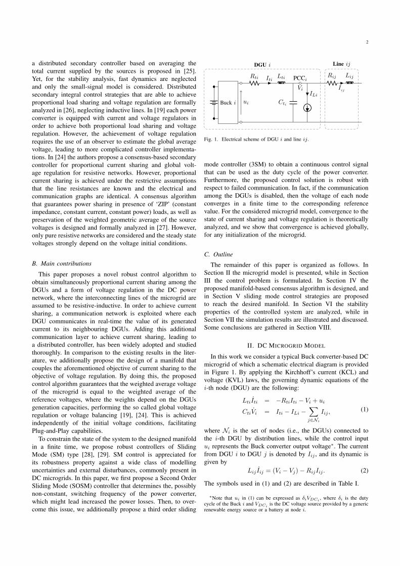
Fig. 1. Electrical scheme of DGU i and line ij.

mode controller (3SM) to obtain a continuous control signalthat can be used as the duty cycle of the power converter.Furthermore, the proposed control solution is robust withrespect to failed communication. In fact, if the communicationamong the DGUs is disabled, then the voltage of each nodeconverges in a finite time to the corresponding referencevalue. For the considered microgrid model, convergence to thestate of current sharing and voltage regulation is theoreticallyanalyzed, and we show that convergence is achieved globally,for any initialization of the microgrid.

C. Outline

The remainder of this paper is organized as follows. InSection II the microgrid model is presented, while in SectionIII the control problem is formulated. In Section IV theproposed manifold-based consensus algorithm is designed, andin Section V sliding mode control strategies are proposedto reach the desired manifold. In Section VI the stabilityproperties of the controlled system are analyzed, while inSection VII the simulation results are illustrated and discussed.Some conclusions are gathered in Section VIII.

II. DC MICROGRID MODEL

In this work we consider a typical Buck converter-based DCmicrogrid of which a schematic electrical diagram is providedin Figure 1. By applying the Kirchhoff’s current (KCL) andvoltage (KVL) laws, the governing dynamic equations of thei-th node (DGU) are the following:

LtiIti = −RtiIti − Vi + ui

CtiVi = Iti − ILi −∑

j∈Ni

Iij , (1)

where Ni is the set of nodes (i.e., the DGUs) connected tothe i-th DGU by distribution lines, while the control inputui represents the Buck converter output voltage∗. The currentfrom DGU i to DGU j is denoted by Iij , and its dynamic isgiven by

Lij Iij = (Vi − Vj)−RijIij . (2)

The symbols used in (1) and (2) are described in Table I.

∗Note that ui in (1) can be expressed as δiVDCi, where δi is the duty

cycle of the Buck i and VDCiis the DC voltage source provided by a generic

renewable energy source or a battery at node i.

3

TABLE IDESCRIPTION OF THE USED SYMBOLS

State variables

Iti Generated currentVi Load voltageIij Exchanged current

Parameters

Rti Filter resistanceLti Filter inductanceCti Shunt capacitorRij Line resistanceLij Line inductance

Inputs

ui Control inputIti Unknown current demand

The overall network is represented by a connected andundirected graph G = (V, E), where the nodes, V = 1, ..., n,represent the DGUs and the edges, E = 1, ...,m, representthe distribution lines interconnecting the DGUs. The networktopology is represented by its corresponding incidence matrixB ∈ Rn×m. The ends of edge k are arbitrarily labeled with a+ and a −, and the entries of B are given by

Bik =

+1 if i is the positive end of k−1 if i is the negative end of k0 otherwise.

Consequently, the overall microgrid system can be writtencompactly for all nodes i ∈ V as

LtIt = −RtIt − V + u

CtV = It + BI − ILLI = −BTV −RI,

(3)

where It, V, IL, u ∈ Rn, and I ∈ Rm. Moreover, Ct, Lt, Rt ∈Rn×n and R,L ∈ Rm×m are positive definite diagonalmatrices, e.g. Rt = diag(Rt1 , . . . , Rtn). To permit the con-troller design in the next sections, the following assumptionis introduced on the available information of the system:

Assumption 1: (Available information) The state variablesIti and Vi are locally available at the i-th DGU. The networkparameters Rt, Lt, Ct, R, L and the current demand IL areconstant and unknown, but with known bounds.

Remark 1: (Varying parameters and current demand) Weassume that the parameters and the current demand are con-stant, to allow for a steady state solution and to theoreticallyanalyze the stability of the microgrid. Yet, the control strategythat we propose in the next sections is applicable even if thisassumption is removed.

Remark 2: (Kron reduction) Note that in (1), the loadcurrents are located at the PCC of each DGU (see alsoFigure 1). This situation is generally obtained by a Kronreduction of the original network, yielding an equivalentrepresentation of the network [26]. It is important to realizethat the network (topology) of the Kron reduced network isgenerally unknown and differs from the original network. It is

therefore desirable that a control structure is independent ofthe underlying distribution network.

III. CURRENT SHARING AND VOLTAGE BALANCING

In this section we make the considered control objectivesexplicit. First, we note that for a given constant control inputu, a steady state solution (It, V , I) to system (3) satisfies

V = −RtIt + u

−BI = It − ILI = −R−1BTV .

(4)

The second line of (4) implies† that at steady state the totalgenerated current 1Tn It is equal to the total current demand1Tn IL. To improve the generation efficiency, it is generallydesired that the total current demand is shared among the var-ious DGUs proportionally to the generation capacity of theircorresponding energy sources (proportional current sharing).This desire can be expressed as wiIti = wjItj for all i, j ∈ V ,where wi relates to the generation capacity of converter i, andleads to the first objective concerning the desired steady statevalue of the generated currents It.

Objective 1: (Proportional Current sharing)

limt→∞

It(t) = It = W−11ni∗t , (5)

with i∗t = 1Tn IL/(1TnW

−11n) ∈ R, W = diagw1, . . . , wn,wi > 0, for all i ∈ V .

Note that (5) indeed satisfies 1Tn It = 1TW−11ni∗t =1Tn IL. From the second and third lines of (4) it follows that thecorresponding steady state voltages V satisfy BR−1BTV =W−11ni∗t−IL, that prescribes the value of the required differ-ences in voltages, BTV , achieving proportional current shar-ing. This admits the freedom to shift all steady state voltageswith the same constant value, since BTV = BT

(V + a1n

),

with a ∈ R any scalar. To define the optimal steady statevoltages, we assume that for every DGU i, there exists adesired reference voltage V ?i .

Assumption 2: (Desired voltages) There exists a constantreference voltage V ?i at the PCC, for all i ∈ V .

Often the values for V ?i are chosen identical for all i ∈ V ,and are set to the desired voltage level of the overall network.Generally, the requirement of current sharing does not permitfor V = V ∗, and might cause voltages deviations from thecorresponding reference values. Then, a reasonable alternativeis to keep the weighted average value of the PCC voltagesat the steady state identical to the weighted average value ofthe desired reference voltages V ? (voltage balancing) [24].Particularly, we choose the weights to be 1/wi, for all i ∈ V ,such that at the converters with a relatively large generationcapacity, there is a relatively small voltage deviation. It isindeed a standard practise that the sources with the largestgeneration capacity determine the grid voltage. Therefore,given a V ?, we aim at designing a controller that, in additionto Objective 1, also guarantees voltage balancing, i.e.,

†The incidence matrix B, satisfies 1TnB = 0, where 1n ∈ Rn is the vectorconsisting of all ones.

4

Objective 2: (Voltage balancing)

limt→∞

1TnW−1V (t) = 1TnW

−1V = 1TnW−1V ?. (6)

Remark 3: (Equal current sharing) Note that by settingin (5) and (6) the weights wi, for all i ∈ V , identical, thetotal current demand is equally shared among the DGUs andthe arithmetic average of the microgrid voltage is equal to thearithmetic average of the voltage references.

By substituting (5) and (6), in (4), one can easily verify thatachieving Objective 1 and Objective 2 prescribes the (optimal)steady state output voltages of the Buck converters, u = uopt.

Lemma 1: (Optimal feedforward input) If system (3), atsteady state, achieves Objective 1 and Objective 2, then thecontrol input u to system (3) is given by

uopt = −(BR−1BT −Ψ

)−1(ΨV ∗ + IL

), (7)

with

Ψ =(In + BR−1BTRt)W−11n1TnW−1

1TnW−1RtW−11n

, (8)

and In ∈ Rn×n the identity matrix.Proof: When Objective 1 and Objective 2 hold, the steady

state of (3) necessarily satisfies

0 = −RtW−11ni∗t − V + uopt

0 = W−11ni∗t − BR−1BTV − IL

0 = 1TnW−1V − 1TnW−1V ∗,

(9)

with i∗t = 1Tn IL/(1TnW

−11n) ∈ R. A tedious, but straight-forward, calculation permits to solve (9) for uopt, yielding (7).

In order to determine (7), exact knowledge of almost allnetwork parameters, as well as the current demand IL, isrequired. Since this information is not available (see alsoAssumption 1), we propose in the next sections distributedcontrollers that, provably, achieve voltage balancing usingonly local measurements of Vi, and that achieve proportionalcurrent sharing by exchanging information on Iti amongneighbours over a communication network. In the remainderof this section we further elaborate on the steady state voltagesimposed by the control objectives.

A. Steady state voltages

First, we notice that it follows from (5) and (9) that thesteady state voltages V satisfy

V = −RtW−11n1Tn IL

1TnW−11n

+ uopt. (10)

From (7) and (10) it is evident that the steady state valuesof the voltages at each node depend on the loads IL and thevoltage references V ?. Since V ? is free to design, it can bepotentially chosen in such a way that too low or too highvoltages are avoided. To help the design of V ?, we show thatthe the steady state voltages V i, for all i ∈ V , are shifted bythe same quantity, when V ? is altered.

Lemma 2: (Voltage shifting property) Let Objective 1 andObjective 2 hold, and let V (1) ∈ Rn denote the steady state

voltage value associated to the voltage reference V ?(1) ∈ Rn.Consider the new voltage reference V ?(2) ∈ Rn and thecorresponding steady state voltage value V (2) ∈ Rn. Then,∆V = V (2) − V (1) satisfies

∆V = 1n1TnW

−1∆V ?

1TnW−11n

, (11)

with ∆V ? = V ?(2) − V ?(1).Proof: When Objective 2 holds, we have

1TnW−1(V (1) + ∆V ) = 1TnW

−1(V ?(1) + ∆V ?), (12)

which implies 1TnW−1∆V = 1TnW

−1∆V ?. Bearing in mindthat the voltage differences between any node of the microgridare prescribed by the achievement of current sharing (see theparagraph below Objective 1), we have BTV (1) = BTV (2),implying ∆V = 1nν, with ν = 1TnW

−1∆V ?/1TnW−11n,

i.e., all the voltages are shifted by the same quantity.Consequently, any node i in the network can lower or

increase its steady state voltage V i, by adjusting its ownreference V ?i . Although, the design and the analysis of avoltage reference generator is postponed to a future research,the property proven in Lemma 2 could be exploited to tune thereferences in order to avoid that the voltages at some nodesare lower or higher than some given thresholds.

IV. A MANIFOLD-BASED CONSENSUS ALGORITHM

In this section we introduce the key aspects of the proposedsolution to simultaneously achieve Objective 1 and Objec-tive 2, consisting of a consensus algorithm and the design of amanifold to where the solutions to the system should converge.First, we augment system (3) with additional state variables(distributed integrators) θi, i ∈ V , with dynamics given by

θi = −∑

j∈N ci

γij(wiIti − wjIti), (13)

where N ci is the set of the DGUs that communicate with the

i-th DGU, γij = γji ∈ R>0 are additional gain constants, andwi, wj ∈ R>0 are constant weights depending on the DGUsgeneration capacity. Let Lc denote the (weighted) Laplacianmatrix associated with the communication graph, which can bedifferent from the topology of the (reduced) microgrid. Then,the dynamics in (13) can be expressed compactly for all nodesi ∈ V as

θ = −LcWIt, (14)

that indeed has the form of a consensus protocol, permitting asteady state where WIt ∈ im(1n) (see also Objective 1). Weimpose the following restrictions on (14):

Assumption 3: (Controller structure) For all i ∈ V , theintegrators states θi are initialized such that 1Tnθ(0) = 0.Furthermore, the graph corresponding to the topology of thecommunication network is undirected and connected.

The most straightforward choice of initialization of the stateθi(0), that satisfies Assumption 3, is to initialize all θi to zero,i.e. θ(0) = 0. Whereas connectedness of the communicationgraph is needed to ensure current sharing among all DGUs,the consequence of the required initialization of θ is that the

5

average value of the entries of θ is preserved and identical tozero for all t ≥ 0, as proved in the following lemma:

Lemma 3: (Preservation of 1Tnθ) Let Assumption 3 hold.Given system (14), the average value 1

n

∑i∈V θi is preserved,

i.e.,1

n1Tnθ(t) =

1

n1Tnθ(0) for all t ≥ 0. (15)

Proof: Pre-multiplying both sides of (14) by 1Tn yields

1Tn θ = −1TnLcWIt = 0, (16)

where 1TnLc = 0, follows from Lc being the Laplacian matrixassociated with an undirected graph.

The fact that 1Tnθ(t) = 0, is essential to the second aspectof the proposed solution, the design of a manifold. Bearing inmind Objective 2, we propose the following desired manifold:

(It, V, I, θ) : W−1(V − V ?)− θ = 0. (17)

Indeed, exploiting the preservation of 1Tnθ, we have on thedesired manifold (17), 1TnW

−1V = 1Tn (θ + W−1V ?) =1TnW

−1V ?. Constraining the solutions to a system to aspecific manifold is typical for sliding mode based controllers,and we will discuss some suitable controller designs in the nextsection.

Remark 4: (Plug-and-Play) The main results in this workassume a constant network topology. Nevertheless, an interest-ing extension is to consider the plugging in or out of variousconverters. The analysis of the corresponding switched/hybridsystem is outside the scope of this work. Here, we merelydescribe how the required initialization θi should be extendedtowards the setting of changing topologies, in order to preservethe crucial property 1Tnθ = 0. First, if a new DGU (sayDGUn+1) wants to join the network, its integrator state isinitialized to zero, i.e., θn+1(tnew) = 0, tnew being the timeinstant when DGUn+1 is plugged-in. Second, if a DGU(say DGU i) is unplugged at the time instant tout, we letθi(t) = θi(tout) for all t > tout, without re-setting anyintegrator. If DGU i wants to join again the network at thetime instant tin > tout, the dynamic of θi is described againby (13) for all t > tin. Since θi(tin) = θi(tout), also the plug-in operation occurs without re-setting any integrator state.

V. SLIDING MODE CONTROLLERS

We now propose a Distributed Second Order Sliding Mode(D-SOSM) control law, and a Distributed Third Order SlidingMode (D-3SM) control law, to steer, in a finite time, the stateof system (3), augmented with (14), to the desired manifold(17). As will be discussed in the coming subsections, thechoice of the particular control law, D-SOSM or D-3SM,depends on the desired implementation.

First, to facilitate the upcoming discussion, we recall thefollowing definitions that are essential to sliding mode control:

Definition 1: (Sliding function) Consider system

x = ζ(x, u), (18)

with state x ∈ Rn, and input u ∈ Rm. The sliding functionσ(x) : Rn → Rm is a sufficiently smooth output function ofsystem (18).

Definition 2: (r–sliding manifold) The r–sliding manifold‡

is given by

x ∈ Rn, u ∈ Rm : σ = Lζσ = · · · = L(r−1)ζ σ = 0, (19)

where L(r−1)ζ σ(x) is the (r−1)-th order Lie derivative of σ(x)

along the vector field ζ(x, u). With a slight abuse of notationwe also write Lζσ(x) = σ(x), and L(2)

ζ σ(x) = σ(x).Definition 3: (r–order sliding mode (controller)) A r–

order sliding mode is enforced from t = Tr ≥ 0, when,starting from an initial condition, the state of (18) reachesthe r–sliding manifold, and remains there for all t ≥ Tr. Theorder of a sliding mode controller is identical to the order ofthe sliding mode that it is aimed at enforcing.

Bearing in mind the definitions above and the desiredmanifold (17), we consider the following sliding functionσ ∈ Rn:

σ(V, θ) = W−1(V − V ?)− θ. (20)

A. Second order SM control: variable switching frequency

Regarding the sliding function (20) as the output function ofsystem (3), (14), it appears that the relative degree§ is two. Thisimplies that a second order sliding mode (SOSM) controllercan be naturally applied in order to make the state of thecontrolled system reach, in a finite time, the sliding manifold(It, V, I, θ) : σ = σ = 0. According to the SOSM controltheory, the auxiliary variables ξ1 = σ and ξ2 = σ have to bedefined, resulting in the so-called auxiliary system

ξ1 = ξ2

ξ2 = b(It, V, I, u) +Gdu.(21)

Taking into account the expressions for σ and σ, a straight-forward calculation shows that, in the auxiliary system (21),the expression for b ∈ Rn is given by

b =−(W−1C−1t + LcW

)L−1t RtIt

−((W−1C−1t + LcW

)L−1t +W−1C−1t BL−1BT

)V

−W−1C−1t BL−1RI −Gau,(22)

and Gd, Ga ∈ Rn×n are

Gd = (W−1C−1t +DcW )L−1t ,

Ga = AcWL−1t .(23)

Here, Dc and Ac are the degree matrix and the adjacencymatrix of the communication graph, respectively, i.e. Lc =Dc−Ac. We assume that the entries of b and Gd have knownbounds for all i ∈ V:

|bi| ≤ bmaxi

Gmini≤ Gdii ≤ Gmaxi

,(24)

with bmaxi, Gmini

and Gmaxibeing positive constants. Ac-

cording to the theory underlying the so-called Suboptimal

‡For the sake of simplicity, the order r of the sliding manifold is omittedin the remainder of this paper.§ The relative degree is the minimum order ρ of the time derivative

σ(ρ)i , i ∈ V , of the sliding variable associated with the i-th node in which

the control ui, i ∈ V explicitly appears.

6

SOSM (SSOSM) control algorithm [30], the i-th SOSMcontrol law, that can be used to steer ξ1i and ξ2i , to zeroin a finite time, even in presence of uncertainties, is given by

ui = −µiUmaxisgn

(ξ1i − 1

2ξmax1i

), (25)

with

Umaxi> max

(bmaxi

µ∗iGmini

;4bmaxi

3Gmini− µ∗iGmaxi

), (26)

µ∗i ∈ (0, 1] ∩(

0,3Gmini

Gmaxi

), (27)

µi switching between µ∗i and 1, according to [30, Algo-rithm 1]. The extremal value ξmax

1i in (25) can be detectedby implementing for instance a peak detector as in [31]. Notethat only the value of ξ1i , i.e., wi(Vi − V ?i )− θi, is requiredto generate the control signal ui.

Remark 5: (Switching frequency) The discontinuous con-trol signal (25) can be directly used in practice to open andclose the switch of the Buck converter. As a result, the In-sulated Gate Bipolar Transistors (IGBTs) switching frequencycannot be a-priori fixed and the power losses could be high.Usually, in order to achieve a constant IGBTs switchingfrequency, Buck converters are controlled by implementingthe so-called Pulse Width Modulation (PWM) technique. Todo this, a continuous control signal, that represents the so-called duty cycle of the Buck converter, is required.

B. Third Order SM control: duty cycle

To ensure a continuous control input (duty cycle), weadopt the procedure suggested in [30] and first integrate the(discontinuous) control signal generated by a sliding modecontroller, yielding for system (3) augmented with (14)

LtIt = −RtIt − V + u

CtV = It + BI − ILLI = −BTV −RIθ = −LcWIt

u = v,

(28)

where v is the new (discontinuous) control input. Note that theinput signal to the converter, u(t) =

∫ t0v(τ)dτ , is continuous,

so that ui can be used as duty cycle for the switch of thei-th Buck converter. A consequence is that the system relativedegree (with respect to the new control input v) is now equalto three, so that we need to rely on a third order slidingmode (3SM) control strategy to reach the sliding manifold(It, V, I, θ) : σ = σ = σ = 0 in a finite time. To do so, wedefine the auxiliary variables ξ1 = σ, ξ2 = σ and ξ3 = σ, andbuild the auxiliary system as follows

ξ1 = ξ2

ξ2 = ξ3

ξ3 = b(It, V, I, u) +Gdv

u = v,

(29)

with b as in (22), and Gd, Ga as in (23). Then, we assumethat the entries of b can be bounded as

|bi(·)| ≤ βmaxi ∀i ∈ V, (30)

where βmaxiis a known positive constant.

Remark 6: (Uncertainty of b, b and Gd) The mappingsb, b and matrix Gd are uncertain due to the presence ofthe unmeasurable current demand IL and possible networkparameter uncertainties. However, relying on Assumption 1and observing that b and b depend on the electric signalsrelated to the finite power of the microgrid, b, b and Gd arein practice bounded. Generally, the bounds of the unknownquantities can be determined by data analysis and engineeringunderstanding.

Now, the 3SM control law proposed in [32] can be used tosteer ξ1i , ξ2i and ξ3i , i ∈ V , to zero in a finite time. It is givenby

vi = −αi

v1i = sgn(σi) σi ∈M1i/M0i

v2i = sgn(σi +

σ2i v1i2αri

)σi ∈M2i/M1i

v3i = sgn(si(σi)) otherwise,(31)

where σi = [σi, σi, σi]T and

si(σi) = σi +σ3i

3α2ri

+ v2i

[1√αri

(v2i σi +

σ2i

2αri

) 32

+σiσiαri

],

withαri = αiGmini

− βmaxi> 0. (32)

Then, given the bounds Gminiand βmaxi

, the control ampli-tude αi is chosen such that αri is positive. The manifoldsM1i , M2i , M3i in (31) are defined as

M0i =σi ∈ R3 : σi = σi = σi = 0

M1i =σi ∈ R3 : σi −

σ3i

6α2ri

= 0, σi +σi|σi|2αri

= 0

M2i =σi ∈ R3 : si(σi) = 0

.

From (31), one can observe that the controller of DGU irequires not only σi, but also σi and σi. Yet, according toAssumption 1, only Iti and Vi are measurable at the i-th DGU.Then, one can rely on Levant’s second-order differentiator [33]to retrieve σi and σi in a finite time. Consequently, forsystem (29), the estimators are given by

˙ξ1i = −λ0i

∣∣∣ξ1i − ξ1i∣∣∣23

sgn(ξ1i − ξ1i

)+ ξ2i

˙ξ2i = −λ1i

∣∣∣ξ2i −˙ξ1i

∣∣∣12

sgn(ξ2i −

˙ξ1i

)+ ξ3i

˙ξ3i = −λ2i sgn

(ξ3i −

˙ξ2i

),

(33)

where ξ1i = σi, ξ2i = ˙σi and ξ3i = ¨σi are the estimatedvalues of ξ1i = σi, ξ2i = σi and ξ3i = σi, respectively.The estimates obtained via (33) can be used in (31), replac-ing the original variables. The other parameters are λ0i =

3Λ1/3i , λ1i = 1.5Λ

1/2i , λ2i = 1.1Λi, Λi > 0, as suggested

in [33].

7

Remark 7: (Scalability and distributed control) Sincethe selected sliding function (20) is designed by using theadditional state θ in (14), the overall control scheme is indeeddistributed, and only information on generated currents Itneeds to be shared. More precisely, the controller of the i-thDGU needs information only from the DGUs that communi-cate with it. Note that the design of the local controller for eachDGU is not based on the knowledge of the whole microgrid,so that the complexity of the control synthesis does not dependon the microgrid size.

Remark 8: (Alternative SM controllers) In this work werely on the SOSM control algorithm proposed in [30] and the3SM control law proposed in [32]. However, the results inthis paper are obtained independent of the particular choice ofsliding mode controller.

VI. STABILITY ANALYSIS

In this section we first show that the states of the controlledmicrogrid are constrained, after a finite time, to the manifoldσ = 0, where Objective 2 is achieved. Thereafter, we provethat the solutions to the system, once the sliding manifold isattained, converge exponentially to a constant point, achievingadditionally Objective 1.

A. Equivalent reduced order system

As a first step, we study the convergence to the slidingmanifold when the SSOSM or the 3SM control law is appliedto the system.

Lemma 4: (Convergence to the sliding manifold: SSOSM)Let Assumption 1 hold. The solutions to system (3) augmentedwith (14), controlled via the SSOSM control law (25), con-verge in a finite time Tr, to the sliding manifold (It, V, I, θ) :σ = σ = 0, with σ given by (20).

Proof: Following [30], the application of (25) to eachconverter guarantees that σ = σ = 0, for all t ≥ Tr.

Lemma 5: (Convergence to the sliding manifold: 3SM)Let Assumption 1 hold. The solutions to system (3) aug-mented with (14), controlled via 3SM control algorithm (29)-(33), converge in a finite time Tr, to the sliding manifold(It, V, I, θ) : σ = σ = σ = 0, with σ given by (20).

Proof: By implementing the Levant’s differentiator (33)in each node, the values of ξ1, ξ2, ξ3, are estimated in a finitetime TLd ≥ 0 [33]. Then, following [32], the applicationof (31) to each converter guarantees that σ = σ = σ = 0,for all t ≥ Tr ≥ TLd.

As we will show in the proof of Theorem 2 in thenext subsection, converging to the sliding manifold whereσ = 0, is sufficient to conclude that Objective 2 (voltagebalancing) is achieved. We postpone the analysis, in orderto show additionally convergence to a constant voltage. Forthe analysis of the system, when the solutions are constrainedto the sliding manifold, it is convenient to exploit the so-called system order reduction property, typical of sliding modecontrol methodology. Indeed, when the state of system (3)augmented with (14) is constrained to the sliding manifold(It, V, I, θ) : σ = σ = 0, with σ given by (20), the con-trolled system is described by 3n+m differential equations and

2n algebraic equations. Then, it is possible to obtain 2n statevariables depending on the other n + m ones. The resultingsystem of order n + m represents the reduced order systemequivalent to the system controlled with a discontinuous law,with the initial condition (It(Tr), V (Tr), I(Tr), θ(Tr)), whenσ = σ = 0.

Lemma 6: (Equivalent reduced order system) For allt ≥ Tr, the dynamics of the controlled system (3) augmentedwith (14) are given by the following equivalent system ofreduced order

CtV =(In − (In + CtWLcW )

−1)BI

−(In − (In + CtWLcW )

−1)IL

LI =− BTV −RI,

(34)

together with the following algebraic relations

θ = W−1 (V − V ?) (35)

It = (In + CtWLcW )−1

(−BI + IL) . (36)

Proof: Given the sliding function (20), by virtue ofLemma 4 and Lemma 5, the state of system (3) augmentedwith (14) is constrained to the manifold (It, V, I, θ) : σ =σ = 0, where θ = W−1 (V − V ?) and V = Wθ. From thelatter, one can straightforwardly obtain (36). After substitutingexpression (36) for It in (3), the dynamics of the voltage Vbecome as in (34).

B. Exponential convergence and objectives attainment

In the pervious subsection, we established that after afinite time Tr, the dynamics of the controlled microgrid aredescribed by the equivalent system (34). In this subsection westudy the convergence properties of this equivalent system. Todo so, we rely on the concept of semistability [34], of whichwe recall the definition for convenience.

Definition 4: (Semistability) Consider the autonomous sys-tem

x(t) = Ax(t), (37)

where t ≥ 0, x ∈ Rn and A ∈ Rn×n. System (37) issemistable if limt→∞ x(t) exists for all initial conditions x(0).

Furthermore, the following lemma turns out to be useful inthe upcoming analysis:

Lemma 7: Given a positive definite matrix P ∈ Rn×n anda positive semidefinite matrix Q ∈ Rn×n, then

P −(P−1 +Q

)−1 0. (38)

Proof: Let Q = P12QP

12 . Clearly, Q 0, and In + Q

0. Then,

P −(P−1 +Q

)−1= P

12

[In −

(In + Q

)−1]P

12 (39)

is a positive semidefinite matrix if and only if In − (In +Q)−1 = Q(In + Q)−1 0. Observing that (In + Q)−1 0,it yields

Q(In + Q)−1 v (In + Q)−12 Q(In + Q)−

12 0, (40)

which completes the proof.

8

Next, we show that the line currents I converge to a constantvalue.

Lemma 8: (Convergence of I) Let Assumptions 1 and2 hold. Given the equivalent reduced order system (34),limt→∞ I(t) exists for all initial conditions I(Tr).

Proof: Let V = V − V and I = I − I be the errorgiven by the difference between the state of system (34) anda steady state value. Then, the dynamics of the correspondingerror system are given by

Ct˙V =

(In − (In + CtWLcW )

−1)BI

L ˙I =− BT V −RI,(41)

From (41), we obtain˙V = C−1t

(In − (In + CtWLcW )

−1)BI

=(C−1t − (Ct + CtWLcWCt)

−1)BI ,

(42)

andL ¨I +R ˙I + BT ˙V = 0. (43)

Substituting expression (42) for ˙V in (43) leads to

L ¨I +R ˙I + BT(C−1t − (Ct + CtWLcWCt)

−1)B

︸ ︷︷ ︸K

I = 0.

(44)Since, by virtue of Lemma 7 (with P = C−1t , Q =CtWLcWCt), C−1t − (Ct + CtWLcWCt)

−1 0, then wealso have K = BT (C−1t − (Ct + CtWLcWCt)

−1)B 0.According to [34, Corollary 2], system (44) is semistable (seeDefinition 4) if and only if

rank

RR(L−1K)R(L−1K)2

...R(L−1K)m−1

= m. (45)

Since R is a positive definite m × m diagonal matrix itcan be readily confirmed that condition (45) holds, such thatsystem (44) is indeed semistable. Since I is a constant vector,it immediately follows that limt→∞ I(t) exists.

Lemma 8 established that limt→∞ I(t) exists for all initialconditions I(Tr). This result can now be exploited to showthat also the voltages converge to constant values.

Lemma 9: (Convergence of V ) Let Assumptions 1–3 hold.Given the equivalent reduced order system (34), limt→∞ V (t)exists for all initial conditions V (Tr).

Proof: Exploiting the convergence of I to a constantvector (see Lemma 8), from (43) we have

limt→∞

BT V (t) = 0, (46)

implying thatlimt→∞

V (t) = 1nκ, (47)

with κ ∈ R. By virtue of Lemma 3 and Lemma 4 or Lemma 5,for all t ≥ Tr, we also have

1TnW−1V = 1Tn (θ +W−1V ?) = 1Tnθ(0) + 1TnW

−1V ?.(48)

Taking the derivative with respect to time on both sides of (48),it follows that 1TnW

−1V (t) = 0 for all t ≥ Tr. Exploiting(47), we obtain

limt→∞

1TnW−1V (t) = 1TnW

−1 limt→∞

V (t)

= 1TnW−11nκ

= 0,

(49)

which implies κ = 0 and consequently that limt→∞ V (t)exists for all initial conditions V (Tr).

We are now ready to establish the first main result of thispaper.

Theorem 1: (Achieving current sharing) Let Assump-tions 1–3 hold. Consider system (3), (14), controlled withthe proposed distributed SSOSM (Subsection V-A) or 3SM(Subsection V-B) control scheme. Then, the generated cur-rents It(t) converge, after a finite time, exponentially toW−11n1Tn IL/(1

TnW

−11n), achieving proportional currentsharing.

Proof: According to Lemma 6, for all t ≥ Tr, thedynamics of the controlled system (3), (14) are given by theautonomous system (34) together with the algebraic equations(35) and (36). Bearing in mind the results proved in Lemma 8and Lemma 9, the dynamics of the line current I and thevoltage V are semistable. From the algebraic equations (35)and (36), it follows that limt→∞ θ(t) and limt→∞ It(t) exist aswell. Since (34) is linear and ker(Lc) = im(1n), (14) impliesthat the vector It(t), with initial condition It(Tr), convergesexponentially to a constant vector, achieving proportionalcurrent sharing.

We now proceed with establishing the second main resultof this paper.

Theorem 2: (Achieving voltage balancing) Let Assump-tions 1–3 hold. Consider system (3), (14), controlled withthe proposed distributed SSOSM (Subsection V-A) or 3SM(Subsection V-B) control scheme. Then, given a desired ref-erences vector V ?, the voltages V (t) satisfy 1TnW

−1V (t) =1TnW

−1V ? for all t ≥ Tr, with Tr a finite time.Proof: Following Lemma 4 or Lemma 5, for all

t ≥ Tr, the equality W−1V (t) = W−1V ? + θ(t) holds.Pre-multiplying both sides by 1Tn yields 1TnW

−1V (t) =1TnW

−1V ? + 1Tnθ(t). Due to Assumption 3 and by virtueof Lemma 3, one has that 1Tnθ(t) = 1Tnθ(0) = 0. Then, onecan conclude that voltage balancing is achieved for all t ≥ Tr.

Remark 9: (Robustness to failed communication) Theproposed control scheme is distributed and as such requires acommunication network to share information on the generatedcurrents. However, note that the integrators θ in (14) are notneeded to regulate the voltages in the microgrid to their desiredvalues, but are only required to achieve current sharing andvoltage balancing. In fact, by omitting the variable θ in theanalysis, the controlled microgrid converges, in a finite time,to the manifold σ = 0, where V = V ?, as shown in [14].Moreover, considering constant value of θi (e.g. after the plug-out of the DGU i), the controlled DGU i converges, in a finitetime, to the manifold σi = 0, where Vi = V ?i + wiθi.

9

V1 V4

V2 V3

L12

R12

L14 R14

R34

L34

R23 L23

DGU 1︷ ︸︸ ︷It1 − IL1

It2 − IL2

It4 − IL4

It3 − IL3

γ12γ23

γ34

Fig. 2. Scheme of the considered (Kron reduced) microgrid with 4 powerconverters. The dashed lines represent the communication network.

TABLE IIMICROGRID PARAMETERS AND CURRENT DEMAND

DGU 1 2 3 4

Rti (Ω) 0.2 0.3 0.5 0.1Lti (mH) 1.8 2.0 3.0 2.2Cti (mF) 2.2 1.9 2.5 1.7wi (–) 0.4−1 0.2−1 0.15−1 0.25−1

V ?i (V) 380.0 380.0 380.0 380.0ILi(0) (A) 30.0 15.0 30.0 26.0∆ILi (A) 10.0 7.0 −10.0 5.0

TABLE IIILINE PARAMETERS

Line 1,2 2,3 3,4 1,4

Rij (mΩ) 70 50 80 60Lij (µH) 2.1 2.3 2.0 1.8

Remark 10: (Perturbations in the controller states) Incase Assumption 3 is violated, we have 1Tnθ(t) = 1Tnθ(0),and consequently 1TnW

−1V (t) = 1TnW−1V ?+1Tnθ(0) on the

sliding manifold, implying that the weighted average voltageof the microgrid is shifted by 1Tnθ(0). However, the presentedstability analysis is still valid such that the stability of thewhole microgrid and the achievement of proportional currentsharing is still guaranteed.

VII. SIMULATION RESULTS

In this section, the proposed manifold-based consensus algo-rithm is assessed in simulation by implementing the third ordersliding mode control strategy discussed in Subsection V-B. Weconsider a microgrid composed of 4 DGUs interconnected asshown in Figure 2, where also the communication network isdepicted. The parameters of each DGU, including the currentdemand, and the line parameters are reported in Tables II andIII, respectively. The weights associated with the edges of thecommunication graph are γ12 = γ23 = γ34 = 10. For all theDGUs the controller parameter αi in (31) is set to 2.4× 103. Inorder to investigate the performance of the proposed controlapproach within a low voltage DC microgrid, four differentscenarios are implemented (see Fig. 3).

A. Scenario 1: proportional current sharing

The system is initially at the steady state. Then, consider acurrent demand variation ∆ILi at the time instant t = 1 s (seeTable II). The PCC voltages and the generated currents areillustrated in Figure 4. One can appreciate that the weighted

average of the PCC voltages (denoted by Vav) is alwaysequal to the weighted average of the corresponding references(see Objective 2), and the current generated by each DGUconverges to the desired value, achieving proportional currentsharing (see Objective 1). Moreover, in Figure 5 the currentsshared among the DGUs are reported together with the controlsignals generated by the 3SM control algorithm (31). Note thatthe 3SM controllers, which require only local measurementsof Vi and information on It from neighbours over the com-munication network, generate control signals that are equal tothe optimal feedforward input (7), without exact knowledgeon the network parameters and the current demand IL.

B. Scenario 2: opening of a distribution line

In the second scenario, we investigate the performance ofthe proposed controllers when a distribution line is opened(e.g. due to an electric fault). The system is initially at thesteady state, and at the time instant t = 0.4 s, the distributionline interconnecting the DGUs 1 and 4 is opened. Then,consider a current demand variation as in Scenario 1. ThePCC voltages and the generated currents are illustrated inFigure 6. One can appreciate that the weighted average of thePCC voltages (denoted by Vav) is always equal to the weightedaverage of the corresponding references (see Objective 2), andthe current generated by each DGU converges to the desiredvalue, achieving proportional current sharing (see Objective 1).Moreover, in Figure 7 the currents shared among the DGUsare reported together with the control signals generated by the3SM control algorithm (31).

C. Scenario 3: plug-out and plug-in of a DGU

In the third scenario, we investigate the Plug-and-Play (PnP)capabilities of the proposed controllers. For the sake of clarity,in this scenario and the next one we consider equal currentsharing among the DGUs. The system is initially at thesteady state, and at the time instant t = 0.4 s, the DGU 4is disconnected from the considered DC network (in thisconfiguration the impedance of the line interconnecting DGU 1and DGU 3 is equal to the sum of the line impedances Z14

and Z34). After a current demand variation as in Scenario 1,at the time instant t = 1.4 s, the DGU 4 is reconnected to theDC network. The PCC voltages and the generated currents areillustrated in Figure 8. One can appreciate that the arithmeticaverage of the PCC voltages (denoted by Vav) is equal tothe arithmetic average of the corresponding references, evenafter disconnecting the DGU 4. Moreover, when the DGU 4operates isolated from the considered DC network, equalcurrent sharing is achieved only among the DGUs 1, 2 and3, while the DGU 4 supplies its local load. However, whenthe DGU 4 is reconnected to the DC network, current sharingamong all the DGUs is again reestablished. Moreover, inFigure 9 the currents shared among the DGUs are reportedtogether with the control signals generated by the 3SM controlalgorithm (31). Note that, when the DGU 4 is isolated from thenetwork, the comparison between u4 and the correspondingoptimal feedforward input loses its meaning.

10

1

2

4

3

Z12

Z14

Z23

Z34

γ12 γ23

γ34

Scenario 1

1

2

4

3

Z12

Z14

Z23

Z34

γ12 γ23

γ34

Scenario 2

1

2

4

3

Z12 Z23

Z34Z14

γ12 γ23

γ34

Scenario 3

1

2

4

3

Z12

Z14

Z23

Z34

γ12 γ23

γ34

Scenario 4

Fig. 3. From the left: the configurations of the considered microgrid implemented in Scenario 1, Scenario 2, Scenario 3 and Scenario 4, respectively.Zij denotes the resistive-inductive impedance of the distribution line interconnecting DGU i with DGU j. Components that are failing/removed during thesimulation are colored red.

0 0.5 1 1.5 2

time (s)

379.5

380

380.5

V(V

)

V1 V2 V3 V4 Vav

0 0.5 1 1.5 2

time (s)

10

20

30

40

50

60

It(A

)

It1 It2 It3 It4 Iti

Fig. 4. Scenario 1. From the top: voltage at the PCC of each DGU togetherwith its weighted average value (dashed line); generated currents together withthe corresponding values (dashed lines) that allow to achieve proportionalcurrent sharing.

0 0.5 1 1.5 2

time (s)

-10

0

10

20

Iij(A

)

I12 I23 I34 I14

0 0.5 1 1.5 2

time (s)

382

384

386

388

390

392

u(V

)

u1 u2 u3 u4 uopt

i

Fig. 5. Scenario 1. From the top: currents shared among the DGUs throughthe lines; control inputs ui(t) =

∫ t0 vi(τ)dτ , vi as in (31), together with the

optimal feedforward inputs (7) indicated by the dashed lines.

0 0.5 1 1.5 2

time (s)

379

379.5

380

380.5

381

381.5

V(V

)V1 V2 V3 V4 Vav

0 0.5 1 1.5 2

time (s)

10

20

30

40

50

60

It(A

)

It1 It2 It3 It4 Iti

Fig. 6. Scenario 2. From the top: voltage at the PCC of each DGU togetherwith its weighted average value (dashed line); generated currents together withthe corresponding values (dashed lines) that allow to achieve proportionalcurrent sharing.

0 0.5 1 1.5 2

time (s)

-10

0

10

20

Iij(A

)

I12 I23 I34 I14

0 0.5 1 1.5 2

time (s)

380

385

390

u(V

)

u1 u2 u3 u4 uopt

i

Fig. 7. Scenario 2. From the top: currents shared among the DGUs throughthe lines; control inputs ui(t) =

∫ t0 vi(τ)dτ , vi as in (31), together with the

optimal feedforward inputs (7) indicated by the dashed lines.

11

0 0.5 1 1.5 2

time (s)

379.5

380

380.5

381

V(V

)

V1 V2 V3 V4 Vav

0 0.5 1 1.5 2

time (s)

25

30

35

It(A

)

It1 It2 It3 It4

Fig. 8. Scenario 3. From the top: voltage at the PCC of each DGU togetherwith its average value (dashed line); generated currents in case of equal currentsharing, which is achieved by DGUs 1, 2, 3 for all the simulation time interval,and by DGU 4 only when it is connected to the microgrid.

0 0.5 1 1.5 2

time (s)

-10

-5

0

5

10

15

Iij(A

)

I12 I23 I34 I14

0 0.5 1 1.5 2

time (s)

380

385

390

395

400

405

u(V

)

u1 u2 u3 u4 uopt

i

Fig. 9. Scenario 3. From the top: currents shared among the DGUs throughthe lines; control inputs ui(t) =

∫ t0 vi(τ)dτ , vi as in (31), together with the

optimal feedforward inputs (7) indicated by the dashed lines.

D. Scenario 4: failing of a communication link

In the last scenario, we investigate the robustness of theproposed controllers to failed communication. The system isinitially at the steady state, and at the time instant t = 0.4 s,the communication between DGU 3 and DGU 4 is interrupted.We observe that as long as the demand does not change,current sharing among all the DGUs in mainteined. The PCCvoltages and the generated currents are illustrated in Figure 10.One can note that after a current demand variation (see TableII), equal current sharing is achieved only among the DGUs1, 2 and 3, while the DGU 4 generates a current such thatthe voltage at node 4 is kept constant. One can appreciatethat the arithmetic average of the PCC voltages (denoted byVav) is equal to the arithmetic average of the correspondingreferences, even after interrupting the communication betweenDGU 3 and DGU 4. Moreover, in Figure 11 the currents shared

0 0.5 1 1.5 2

time (s)

379.5

380

380.5

V(V

)

V1 V2 V3 V4 Vav

0 0.5 1 1.5 2

time (s)

25

30

35

It(A

)

It1 It2 It3 It4

Fig. 10. Scenario 4. From the top: voltage at the PCC of each DGU togetherwith its average value (dashed line); generated currents in case of equal currentsharing, which is achieved by DGUs 1, 2, 3 for all the simulation time interval,and by DGU 4 only before the failing of the communication link.

0 0.5 1 1.5 2

time (s)

-10

-5

0

5

10

15

Iij(A

)

I12 I23 I34 I14

0 0.5 1 1.5 2

time (s)

380

385

390

395

400

u(V

)

u1 u2 u3 u4 uopt

i

Fig. 11. Scenario 4. From the top: currents shared among the DGUs throughthe lines; control inputs ui(t) =

∫ t0 vi(τ)dτ , vi as in (31), together with the

optimal feedforward inputs (7) indicated by the dashed lines.

among the DGUs are reported together with the control signalsgenerated by the 3SM control algorithm (31). Note that, whenthe communication with DGU 4 fails, the comparison betweenu4 and the corresponding optimal feedforward input loses itsmeaning.

Even if IEEE Standards or guidlines for DC power distribu-tion networks do not exist yet (to the best of our knowledge), itis usually required in practical cases that the voltage deviationsare within the 5 % of the desired value (see for instance [24]).In all the previous scenarios, the voltage at the PCC of eachDGU is within the range 380±1 V, implying that the voltagedeviations are less than the 0.3 % of the nominal value V ? =380 V, even during transients and critical conditions.

12

VIII. CONCLUSIONS

In this paper we design a distributed control algorithm,obtaining proportional current sharing and voltage regulationin DC microgrids. Its convergence properties are analyticallyinvestigated. The proposed control scheme exploits a com-munication network to achieve proportional current sharingusing a consensus-like algorithm. Another useful feature ofthe proposed control scheme is that the weighted averagevoltage of the microgrid converges to the weighted averageof the voltage references, independently of the initial voltageconditions. The latter is achieved by constraining the systemto a suitable manifold. To ensure that the desired manifoldis reached in a finite time, even in presence of modellinguncertainties, two sliding mode control strategies are proposed,that provide the switching frequencies or the duty cycle ofthe power converters. An extensive simulation analysis isalso provided, considering different and realistic scenarios.The proposed controllers show satisfactory closed-loop per-formance and Plug-and-Play capabilities, even in presence ofuncertainties, topology changes and communication failings.Interesting future research includes the design of distributedcontrollers aimed at guaranteeing power sharing and studyingthe stability analysis of the resulting nonlinear system.

REFERENCES

[1] S. Trip, M. Cucuzzella, C. De Persis, X. Cheng, and A. Ferrara, “Slidingmodes for voltage regulation and current sharing in DC microgrids,” inProc. American Control Conference, Milwaukee, WI, USA, 2018.

[2] R. Lasseter and P. Paigi, “Microgrid: a conceptual solution,” in Proc.35th IEEE Power Electronics Specialists Conf., vol. 6, Aachen, Ger-many, June 2004, pp. 4285–4290.

[3] M. S. Sadabadi, Q. Shafiee, and A. Karimi, “Plug-and-play voltage sta-bilization in inverter-interfaced microgrids via a robust control strategy,”IEEE Transactions on Control Systems Technology, vol. 25, no. 3, pp.781–791, May 2017.

[4] S. Trip, M. Burger, and C. De Persis, “An internal model approachto frequency regulation in inverter-based microgrids with time-varyingvoltages,” in Proc. of the 53rd IEEE Conference on Decision and Control(CDC), Dec. 2014, pp. 223–228.

[5] M. Cucuzzella, G. P. Incremona, and A. Ferrara, “Decentralized slidingmode control of islanded ac microgrids with arbitrary topology,” IEEETransactions on Industrial Electronics, vol. 64, no. 8, pp. 6706–6713,Apr. 2017.

[6] C. De Persis and N. Monshizadeh, “Bregman storage functions formicrogrid control,” IEEE Transactions on Automatic Control, vol. 63,no. 1, pp. 53–68, Jan. 2018.

[7] J. M. Guerrero, P. C. Loh, T. L. Lee, and M. Chandorkar, “Advancedcontrol architectures for intelligent microgrids - part II: Power quality,energy storage, and AC/DC microgrids,” IEEE Transactions on Indus-trial Electronics, vol. 60, no. 4, pp. 1263–1270, Apr. 2013.

[8] J. J. Justo, F. Mwasilu, J. Lee, and J.-W. Jung, “AC-microgrids versusDC-microgrids with distributed energy resources: A review,” RenewableSustain. Energy Rev., vol. 24, pp. 387–405, Aug. 2013.

[9] X. Liu, P. Wang, and P. C. Loh, “A hybrid AC/DC microgrid and itscoordination control,” IEEE Transactions on Smart Grid, vol. 2, no. 2,pp. 278–286, June 2011.

[10] E. Benedito, D. del Puerto-Flores, A. Doria-Cerezo, O. van der Feltz, andJ. M. A. Scherpen, “Strictly convex loss functions for port-Hamiltonianbased optimization algorithm for MTDC networks,” in Proc. of the 55thIEEE Conference on Decision and Control (CDC), Dec 2016, pp. 7483–7488.

[11] M. Andreasson, R. Wiget, D. V. Dimarogonas, K. H. Johansson, andG. Andersson, “Distributed frequency control through MTDC transmis-sion systems,” IEEE Transactions on Power Systems, vol. 32, no. 1, pp.250–260, 2017.

[12] D. Zonetti, R. Ortega, and J. Schiffer, “A tool for stability and powersharing analysis of a generalized class of droop controllers for high-voltage direct-current transmission systems,” IEEE Transactions onControl of Network Systems, Mar. 2017.

[13] N. Flourentzou, V. G. Agelidis, and G. D. Demetriades, “VSC-basedHVDC power transmission systems: An overview,” IEEE Transactionson Power Electronics, vol. 24, no. 3, pp. 592–602, Mar. 2009.

[14] M. Cucuzzella, S. Rosti, A. Cavallo, and A. Ferrara, “Decentralizedsliding mode voltage control in DC microgrids,” in Proc. of the AmericanControl Conference (ACC), Seattle, WA, USA, May 2017, pp. 3445–3450.

[15] M. Tucci, S. Riverso, and G. Ferrari-Trecate, “Line-independent plug-and-play controllers for voltage stabilization in DC microgrids,” IEEETransactions on Control Systems Technology, vol. 26, no. 3, pp. 1115–1123, May 2017.

[16] M. S. Sadabadi, Q. Shafiee, and A. Karimi, “Plug-and-play robustvoltage control of DC microgrids,” IEEE Transactions on Smart Grid,2017.

[17] M. Cucuzzella, R. Lazzari, S. Trip, S. Rosti, C. Sandroni, and A. Ferrara,“Sliding mode voltage control of boost converters in DC microgrids,”Control Engineering Practice, vol. 73, pp. 161–170, 2018.

[18] J. M. Guerrero, J. C. Vasquez, J. Matas, L. G. de Vicuna, and M. Castilla,“Hierarchical control of droop-controlled AC and DC microgrids –a general approach toward standardization,” IEEE Transactions onIndustrial Electronics, vol. 58, no. 1, pp. 158–172, Jan. 2011.

[19] V. Nasirian, S. Moayedi, A. Davoudi, and F. L. Lewis, “Distributedcooperative control of DC microgrids,” IEEE Transactions on PowerElectronics, vol. 30, no. 4, pp. 2288–2303, Apr. 2015.

[20] V. Nasirian, A. Davoudi, F. L. Lewis, and J. M. Guerrero, “Distributedadaptive droop control for DC distribution systems,” IEEE Transactionson Energy Conversion, vol. 29, no. 4, pp. 944–956, Dec. 2014.

[21] S. Peyghami-Akhuleh, H. Mokhtari, P. Davari, P. C. Loh, and F. Blaab-jerg, “A new secondary control approach for voltage regulation in DCmicrogrids,” in 2016 IEEE Energy Conversion Congress and Exposition(ECCE), Sept. 2016, pp. 1–6.

[22] S. Sahoo and S. Mishra, “A distributed finite-time secondary averagevoltage regulation and current sharing controller for DC microgrids,”IEEE Transactions on Smart Grid, 2017.

[23] P. Prajof, Y. Goyal, and V. Agarwal, “A novel communication basedaverage voltage regulation scheme for a droop controlled DC microgrid,”IEEE Transactions on Smart Grid, 2017.

[24] M. Tucci, L. Meng, J. M. Guerrero, and G. Ferrari-Trecate, “Aconsensus-based secondary control layer for stable current sharing andvoltage balancing in DC microgrids,” arXiv preprint, Mar. 2016.

[25] S. Anand, B. G. Fernandes, and J. Guerrero, “Distributed control toensure proportional load sharing and improve voltage regulation inlow-voltage DC microgrids,” IEEE Transactions on Power Electronics,vol. 28, no. 4, pp. 1900–1913, Apr. 2013.

[26] J. Zhao and F. Dorfler, “Distributed control and optimization in DCmicrogrids,” Automatica, vol. 61, pp. 18–26, Nov. 2015.

[27] C. De Persis, E. R. Weitenberg, and F. Dorfler, “A power consensusalgorithm for dc microgrids,” Automatica, vol. 89, pp. 364–375, 2018.

[28] V. I. Utkin, Sliding Modes in Control and Optimization. Springer-Verlag, 1992.

[29] X.-G. Yan, S. K. Spurgeon, and C. Edwards, “Application of de-centralised sliding mode control to multimachine power systems,” inVariable Structure Control of Complex Systems. Springer, 2017, pp.297–313.

[30] G. Bartolini, A. Ferrara, and E. Usai, “Chattering avoidance by second-order sliding mode control,” IEEE Transactions on Automatic Control,vol. 43, no. 2, pp. 241–246, Feb. 1998.

[31] ——, “On boundary layer dimension reduction in sliding mode controlof SISO uncertain nonlinear systems,” in Proc. of the IEEE InternationConference on Control Applications, vol. 1, Trieste, Italy, Sept. 1998,pp. 242–247.

[32] F. Dinuzzo and A. Ferrara, “Higher order sliding mode controllers withoptimal reaching,” IEEE Trans. Automat. Control, vol. 54, no. 9, pp.2126–2136, Sept. 2009.

[33] A. Levant, “Higher-order sliding modes, differentiation and output-feedback control,” Int. J. Control, vol. 76, no. 9-10, pp. 924–941, Jan.2003.

[34] D. Bernstein and S. Bhat, “Lyapunov stability, semistability, and asymp-totic stability of matrix second-order systems,” Journal of Vibration andAcoustics, vol. 117, no. B, pp. 145–153, June 1995.